Abstract

We test implications of economic geography models for location,size and growth of cities with US Census data for 1900 – 1990. Ourtests involve non-parametric estimations of stochastic kernels forthe distributions of city sizes and growth rates, conditional onvarious measures of market potential and on features sizes ofneighbors. We show that while these relationships change duringthe twentieth century, by 1990 they stabilize such that the size dis-tribution of cities conditional on a range of spatial variables are allroughly independent of these conditioning variables. In contrast,similar results suggest that there is a spatial element to the citywage distribution. Our parametric estimations for growth ratesagainst market potential, entry of neighbors, and own laggedpopulation imply a negative effect of market potential on growthrates, unless own lagged population is also included, in whichcase market potential has a positive effect and own lagged popu-lation a negative one. Cities grow faster when they are small rel-ative to their market potential. In total, our results support sometheoretical predictions, but also provide a number of interestingpuzzles.

This paper was produced as part of the Centre’sGlobalisation Programme

Spatial Evolution of the US Urban System

Yannis Ioannides and Henry G. Overman

November 2000

Published byCentre for Economic PerformanceLondon School of Economics and Political ScienceHoughton StreetLondon wc2a 2ae

© Yannis Ioannides and Henry G. Overman, 2000

isbn 0 7530 1426 2

Individual copy price: £5

Spatial Evolution of the US Urban System

Yannis Ioannides and Henry G. Overman

1 Introduction 1

2 Analytical Description and Notation 3

3 Data 5

4 The Number and Location of Cities 6

5 Spatial Features of the US Urban System 8

5.1 First nature and city size . . . . . . . . . . . . . . . . . . . . . . . . . . . . . . . . . . . . . 8

5.2 Second nature and city size . . . . . . . . . . . . . . . . . . . . . . . . . . . . . . . . . . . 9

5.3 Stochastic Kernels for City Sizes . . . . . . . . . . . . . . . . . . . . . . . . . . . . . . . . . 11

6 Growth and the Spatial Structure of the Urban System. 14

6.1 Parametric results . . . . . . . . . . . . . . . . . . . . . . . . . . . . . . . . . . . . . . . . . 16

7 Conclusions 18

The Centre for Economic Performance is financed by the Economic and Social Research Council

Acknowledgements

Ioannides acknowledges generous research support from John D.and Catherine T. MacArthur Foundation and the National ScienceFoundation. Overman acknowledges support from the UK Eco-nomic and Social Research Council. We thank Danny T. Quahfor giving us access to his tSrF package, and Richard Arnott, RobAxtell, Duncan Black, Gilles Duranton, Ed Glaeser, Anna Hard-man, Michael Murray, Diego Puga, Atsushi Yoshida and otherseminar participants at Brookings, Harvard, Kyoto University andthe University of Toronto for their comments; Nick Gill and TimHarris for research assistance and Duncan Black and Linda H.Dobkins for access to data.

Spatial Evolution of the US Urban System

Yannis Ioannides and Henry G. Overman

1. Introduction

As a system of cities develops, existing cities grow and new metropolitan areas form and growat varying rates. Questions pertaining to the location of economic activity, to the relative sizes ofcities in different countries, and to changing roles for different geographical areas in the processof economic growth have attracted renewed interest recently. The theorists who have developedthe so-called new economic geography, including Masahisa Fujita, Paul Krugman and AnthonyVenables [Fujita, Krugman and Venables (1999)], have added important new spatial insights tothe established literature on systems of cities, represented most notably by the work of J. VernonHenderson [Henderson (1974; 1988)]. The system of cities approach featured powerful modelsof intra-metropolitan spatial structure, but lacked an explicit model of inter-metropolitan spatialstructure. Subsequently, inter-metropolitan spatial structure played a key role in the new economicgeography literature, starting with the work of Paul Krugman [Krugman (1991)].1

While theoretical work on the spatial nature of the urban system has expanded rapidly inrecent years, our knowledge about actual spatial features of the urban system pertains mostly tointra-metropolitan spatial structure. Our understanding of spatial features of inter-metropolitanrelationships remains, at best, limited. The present paper seeks to address this imbalance, taking abroad view of temporal cum spatial interactions by estimating models of joint dynamic and spatialinterdependence. Our results build directly on earlier empirical work by Dobkins and Ioannides(1998) and Black and Henderson (1999). However, in contrast to that earlier work, our focus isprimarily on characterising the details of the spatial features of the urban system.

Theoretical reasoning has identified three fundamental features of any given location – the first,second and third “natures” – that determine the extent of development at that location. Firstnature features are those that are intrinsic to the site itself, independent of any development thatmay previously have occurred there. For example, locations on navigable rivers, with favourableclimates have first nature features that might encourage development. The second nature featuresof a location are those that are dependent on the spatial structure of the economic system and notinherent to the location itself. For example, the benefits of good access to a large market would beclassified as a second nature feature of a location. Finally, third nature features of a location are thosethat are dependent on previous development at that location. For example, the availability of localspecialist suppliers might encourage development of activity that uses those specialist suppliers.2

The evidence that we consider here predominantly relates to the importance of second and thirdnature features in understanding the evolution of the urban system. As we suggested earlier, this

1Tabuchi (1998) sets out to synthesise the older system of cities literature with the more recent economic geographybased theories by incorporating intra-metropolitan commuting costs as well as inter-metropolitan transport costs.

2The term first vs. second nature is due to Krugman (1993). A more standard classification might include these thirdnature features as second nature. We separate them here to aid the exposition that follows.

issue has received relatively little attention in the empirical literature, but it is fundamental to ourunderstanding of the urban system.

Krugman-type economic geography models of urban development remain relatively unex-plored empirically. Hanson (2000) and Thomas (1996) are arguably the only exceptions. Bothuse Krugman (1991) as a starting point, modifying it in order to incorporate diseconomies fromcongestion and to develop estimable models. Hanson (2000) estimates a new economic geographytype model using data from US counties. The parameter estimates that he obtains are plausible,but as with all such calibration exercises, it is unclear to what extent this is actually a test of theunderlying model.

Dobkins and Ioannides (1998) examine the basic dynamics of spatial interactions among UScities and its impact on their populations. They use some of the predictions offered by Fujita,Krugman and Venables (1999) and US Census data for metro areas, which span this century from1900 to 1990, to look at patterns of city growth and the distribution of city sizes as new cities enterthe distribution. They emphasise that entry of new cities along with spatial expansion are importantcharacteristics of the United States system of cities. Key spatial characteristics they consider are thepresence of neighboring cities, regional influence, and distance between a city and the nearest onein a higher tier. They find that among cities which enter the system, larger cities are more likelyto locate near other cities. Moreover, older cities are more likely to have neighbors. Distance fromthe nearest higher-tier city is not always a significant determinant of size and growth. They findno evidence of persistent nonlinear effects on urban growth of either size or distance, althoughdistance is important for city size for some years.

Black and Henderson (1999) consider the importance of both first and second nature geographyin explaining the growth rates of cities. They find that both factors are important in explaining citygrowth. In contrast to their paper, we consider a much broader range of issues relating to secondnature characteristics, and sidestep first nature characteristics.

The evidence that we consider falls in to two broad categories. The first relates to the location ofcities. The second to the size and growth of cities. The paper is structured as follows. In section 2 weintroduce the key theoretical concepts relating to the evolution of city sizes, and provide notationwith which to structure our empirical work. In section 3 we describe the data that we use. In section4 we consider spatial features of the location of cities. Assuming that first nature characteristicsare randomly distributed, allows us to test for the importance of second nature characteristics byconsidering the degree of randomness of the location of cities. We conduct nearest neighbor teststo see whether second nature characteristics are sufficient to distort city locations so as to be non-random. In section 5 we examine spatial elements of the city size distribution. We start by taking analternative perspective on the relationship between first nature characteristics and city size. Ratherthan defining specific characteristics to capture good first nature locations, we argue that the bestsites should be settled first. In this case, city size should be positively related to date of settlement.Next, we use a non-parametric approach to consider the relationship between city size and thespatial location of economic activity. We then use a parametric approach to consider the samerelationship. This parametric approach also allows us to examine whether there is a second natureelement to the entry of new cities. Finally, section 7 relates our findings to specific theoretical

2

models and concludes.

2. Analytical Description and Notation

In this section, we briefly outline the theoretical issues underlying our empirical analysis. Let Idenote a set of names of cities, i.e., i = 1, denotes Abilene TX, i = 206 denotes New York, NY, etc.Let It denote the set of cities extant at time t : It ⊆ I , Let It = |It|. Let Pit denote the size, in termsof population (or employment), of city i at time t, i ∈ It, 1 ≤ i ≤ It, and time periods t = 1, . . . T.Let Pt denote the vector of sizes of the It cities in existence in the economy at time t, Pt ∈ RIt

+, andP̄t total population in the economy.

Next we introduce geography. Let ς denote the set of geographical sites, ς = {1, . . . , s, . . . , S},defined within a particular geography, such as the real line (or an interval thereof), a circle, aone-dimensional or a two-dimensional lattice, or simply the North American landscape. Thisdescription allows us to refer to distances between two cities i and j, which for simplicity we taketo be the geodesic distances, Dij. We assume that not all potential urban sites need be occupiedat any time t, and that there is plenty of space for new urban development: maxt : It < |ς|. Aparticular attribute of geography that we use in this paper is the notion of a city’s nearest neighbor,ν(i), which is defined in terms of geodesic distance as follows: dit = min{Dij : i, j ∈ It, i �= j} isthe distance to the nearest neighbor, and ν(i) = {j : Dij ≤ Dik, j, k �= i}, the nearest neighbor. Wenote that because of the evolution of urban system, both these concepts are time-varying.

We define a settlement mapping, gt : ς → {0, It} , where gt(s) = 0, denotes that site s,s ∈ ς, is not settled at time t, and gt(s), if site s is settled, gt(s) �= 0, denotes the site occupiedby city gt(s) ∈ It. We keep track of the evolution of settlement sites by means of the vectorGt = (gt(1), . . . , gt(s), . . . , gt(S)). Once settled and for as long as it remains settled, a site isindistinguishable from the city which occupies it. We refer to the time that site s of city i = gt(s)was first settled, ts

i , as the settlement date.3 A city may disappear, that is, ghost-towns are possible,though relatively rare in the United States during the twentieth century, and not a feature of ourdata, due to the size cutoff.

We define a system of cities in a dynamic setting. We first take the set and location of citiesin each period as given, (It, gt), and postpone until later the issue of entry of new cities.4 Therichness and complexity of theories of urban growth, whether they are of the system-of-citiesgenre [Henderson (1974)], or of the new economic geography variety [Fujita et al. (1999)], makeit hard to obtain specific predictions that are testable by means of our data on emergence of newcities and their sites, populations and wages, and a number of additional characteristics on whichwe elaborate further below. However, new economic geography models, with their emphasis onnational space, as opposed to the intra-metropolitan one of the earlier theories, lend themselvesbetter to overall descriptions of the spatial evolution of the urban system as a whole, and it is

3The settlement date may be different from the time a city enters the data, ei, because of our definition of a city ispredicated on a settlement’s surpassing the population threshold of 50,000. See section 3 for the definition of settlementdates.

4In our parametric analysis below, we consider the impact upon a city’s growth from the entry of neighboring cities.In contrast, Dobkins and Ioannides (1998) examine the geographic patterns of new entrants and the impact of neighborson city growth, where neighbors are construed in the sense of adjacency.

3

for this reason that we appeal to the simplified version of the general theory in Fujita, Krugmanand Venables regarding, in particular, the emergence of new cities. That is, working from theirChapter 8 rather than Chapters 9–10, we can see that an existing city’s new neighbors must havesize exceeding a critical value, if they are to grow. The critical value depends in a highly nonlinearfashion on the existing city’s population and on the various parameters, including in particular thesize of the existing city’s hinterland. We note that all this applies just as well to the case where anexisting city that already has neighbors acquires a new neighbor. Fujita et al. also predict that thedistance between two cities in a linear geography tends to a constant as the number of identicalcities grows. However, different spatial patterns are likely to emerge when cities are different andform a hierarchy [ibid., Ch. 11]. Furthermore, discontinuities in the landscape strengthen the roleof cities’ agglomeration shadows, as discussed in [ibid., Ch. 13]. Finally, the nonlinearity of thedynamics of the setting makes it likely that the urban system exhibits asymmetric behavior whennew cities emerge. The impact of changes in the system upon an individual city is different beforeand after the emergence of neighbors and/or other dramatic changes in the urban landscape.5

Therefore, emergence of a city depends on national geography and the structure of transport costs,and is triggered by exogenous events, such as population growth, or by labor-saving technologicalchange.

Once a particular site is settled, its presence may skew further development in its vicinity inits favor, via its “agglomeration shadow” [Krugman (1996)]. Therefore, the availability of data onthe time of settlement may help anchor the original location of economic activity in an otherwisehomogeneous setting. Of course, the fact that a particular site has already been settled may itselfimply that the site is particularly advantageous in a first-nature sense. Subsequent shocks may causereallocations of economic activity, that is to say second-nature changes, which may bring into thepicture the full force of the asymmetric nature of nonlinear dynamics. The agglomeration shadowof existing cities implies that the earlier a site has been settled, the more likely a city is to grow,regardless of the specific reasons for which a site has been settled in the first place.

Exposition in the remainder of the paper is facilitated by means of a concise description of thespatial evolution of the urban system as follows. Let Ψt be a random function, defined in thespace of Borel-measurable functions B, and let Tt be a sequence of mappings, defined as follows:Tt : I × {0, I} × RI

+ × RI+ ×B −→ I × {0, I} × RI

+ × RI+

(It, Gt; Pt, Wt) = Tt(It−1, Gt−1; Pt−1, Wt−1; Ψt). (1)

This system of equations describes the co-evolution of new and existing cities, It, the determ-ination of the sites they occupy, Gt, and their populations and wages (Pt, Wt). It is, of course,highly nonlinear and expresses bifurcations, as when new cities emerge. Unfortunately, as all ofthe principal contributors in this area acknowledge, it is not possible to derive explicit analyticalresults, even in the case of a constant number of cities [c.f., Krugman (1992); Fujita et al., op. cit.

]. Whereas many of those analysts have resorted to simulations to obtain accurate but numericaldescriptions of results, we take some of those ideas to empirical work. Equations (1) form the basisfor descriptions of the spatial evolution of the urban system outlined below.

5 This is due to the fact that the sustain point and the break point differ [ibid., Ch. 3], a critical implication of nonlinearityof at least third-degree.

4

The highly non-linear nature of the evolution of the urban system, as captured in equation1, justifies the main empirical approach that we adopt below. In such a system, no city is trulyrepresentative of the entire distribution of cities. Standard parametric tools rely on the assumptionthat there is some average (representative) unit whose outcomes can be modelled in a concise wayas the function of a limited number of variables and unknown parameters. According to equation1 such an assumption may not be valid when explaining both the location and size of cities. Ourempirical work on the location of cities, and the approach that we use to characterise the evolutionof the city size distribution do not rely on this representative agent assumption. Instead, we usenon-parametric tools that specifically allow for non-linearities in the evolution of the urban system.

3. Data

There are a variety of ways to define cities empirically. In this paper we use contemporaneousCensus Bureau definitions of metropolitan areas, whenever possible. From 1900 to 1950, we usemetropolitan areas as they were defined by the 1950 census. For years before 1950, we use Bogue’sreconstructions of what each metro area’s population would have been with the metropolitan areasdefined as they were in 1950 [Bogue (1953)]. From 1950 to 1980, we use the metropolitan areadefinitions that were in effect for those years. However, between 1980 and 1990, the Census Bureauredefined metropolitan areas. The effect of the redefinitions were that the largest U.S. cities took ahuge jump in size, and several major cities were split into separate metro areas. While this might beappropriate for some uses of the data, it would introduce “artificial” differences in growth patternsfor the 1980–1990 period. Therefore, we reconstructed the metro areas for 1990, based on the 1980

definitions, much as Bogue did earlier. We believe that this gives us the most consistent definitionsof US cities (metropolitan areas) that we are likely to find.

The method raises a question as to which cities, as defined or reconstructed, should be included.In the years from 1950 to 1980, we use the Census Bureau’s listing of metropolitan areas. Althoughthe wording of the definitions of metropolitan areas has changed slightly over the years, thenumber 50,000 is minimum requirement for a core area within the metropolitan area. Therefore,we used 50,000 as the cutoff for including metropolitan areas as defined by Bogue prior to 1950.Consequently we have a changing number of cities over time, from 112 in 1900 to 334 in 1990.While it is often difficult to deal with an increasing number of cities econometrically, we think thatthis is a key aspect of the US system of cities.

Data on earnings in all cities in the sample for all years are drawn from Census reports. Regionallocation is according to the Census Bureau division of the country into nine regions. Kim (1997)argues that the census regions are likely to serve well as economic regions, at least over the firsthalf of the century.6 Finally, we use the date of settlement for each city, as obtained by Dobkinsand Ioannides, op. cit.. At first glance, one would suppose that the east to west settlement of thecountry would determine settlement dates, but we find early settlement dates in the west and late

6Kim (1997), p. 7–9, discusses the original intention of the definition of U.S. regions as delineating areas of homo-geneous topography, climate, rainfall and soil, but subject to requirement that they not break up states. By design,the definitions were particularly suitable for agriculture and resource-based economies. The role of those industries asinputs to manufacturing would make them likely to serve well as economic regions.

5

ones along the east coast. Settlement here refers to historical references to settlement in a location,and our variable is compiled by sifting through historical texts.7

4. The Number and Location of Cities

This section deals with issues pertaining to the number and location of cities. First, we consider the‘spacing’ of cities by examining the evolution of average bilateral distances between cities relativeto the average distance among nearest neighbors. Referring to Table 3, as the former rises from802.5 miles 1900 to 1005 miles in 1990, (not surprisingly as the US urban system expanded over theNorth American land mass) by nearly 25%, the latter falls by 35%. The dispersion of the formerdeclines while that of the latter slightly grows, as evidenced by the coefficient of variation andnonparametric densities that we have estimated but do not report here. Both those distributionsbecome more symmetric, as evidenced by the ratio of medians to means and the nonparametricdensities. The US urban system both expands and thickens during the twentieth century. Thefrequency distribution of bilateral distances is unimodal, although with a considerable upper tail.

Next, we consider whether the urban system has evolved such that the location of cities is non-random. When considering the location of cities, we need only consider the importance of firstand second nature features of potential city sites. Third nature forces only arise after the city isestablished. If we assume that the distribution of first nature features is essentially random, in thesense that there are a large number of potentially good sites, then we can test for the importanceof second nature in determining city location by considering whether the distribution of cities israndom8. In terms of equation 1, under the null hypothesis of randomness, we can separate out forthe function determining the set of occupied sites. That is:

H0 : (Gt) = T 1t (Ψt) independent of (It, Pt, Wt, It−1, Gt−1Pt−1, Wt−1). (2)

There are many senses in which the location of cities can be non-random. In this section, weconsider a sufficient test for non-randomness first proposed by Clark and Evans (1954). The basicidea is to assume that some underlying spatial probability process determines the distribution ofcities and then to compare the distance between cities to the distance that we would expect, if citieswere located randomly according to this distribution. Although a full matrix of intercity distancesis available9, Clark and Evans (1954) show that a “sufficient” test of non-randomness can be based

7 In a number of cases, the dates are references to military forts. We use those dates because often the site of the fortdetermined the site of the city that grew up nearby. The earliest date is that of Jacksonville, Florida, in 1564, and thelatest is Richland, Washington, originally the site of a nuclear facility settled in 1944. It is an interesting statistic in and ofitself to see how age of settlement correlates with city size.

8This test on the randomness of the location of cities as complementary to that of Ellison and Glaeser (1997) onwhether or not the location of industrial plants is random, conditional on the distribution of population across cities.

9These are calculated on the basis of great circle distances. For any two locations A and B, we can calculate the angleformed by a ray joining the two points A and B and a ray joining A to the centre of the earth as follows:

angle = (sin(latA) × sin(latB)) + (cos(latA) × cos(latB) × cos(longA − longB)) ,

where latA and longA are the latitude and longitude of location A measured in radians. Similarly for latB and longB.For cities, they are the latitudes and longitudes given in the 1999 Times World Atlas. For counties they are the latitudesand longitudes of the largest human settlement.

6

on the distance to nearest neighbor city10. However, even if location of cities is non-random, wemay fail to reject the null-hypothesis of randomness. Non-randomness might be manifested inhigher dimensions than the distance to nearest neighbor.11

Define dA as the actual mean nearest neighbor distance, dA = d̄i; dE = E [d̄i] as the expec-ted mean nearest neighbor distance; σ2(dE) as the expected variance of mean nearest neighbordistance; ρ as the density of cities; and I as the number of cities. Then the Clark-Evans test fornon-randomness is based on the simple test statistic CE = (dA − dE)/σ(dE) which is distributedasymptotically N(0, 1). To calculate the statistic, we need to make a specific assumption on thespatial probability process that governs the random location of cities. We assume that cities arerandomly distributed according to a spatial Poisson process where the probability of a city locatingin any given area is proportional to that area12. For a spatial Poisson distribution the expectedmean nearest neighbor distance, dE = 1/2

√ρ and the variance is σ(dE) = 0.26136/(

√Iρ).

Table 4 shows the results for the US as a whole for each of the census years. The final columnreports R = dA/dE, the ratio of actual to expected distance. A number less than one indicates thatcities are closer together than would be expected if they were randomly located. Conversely, anumber greater than one indicates that cities are further apart than would be expected if they wererandomly located. The N(0, 1) column then tells us whether this departure from randomness issignificant. From the table, we see that US cities are spaced closer than we would expect if theywere randomly located, but that this non-randomness is only significant at the beginning of thecentury. We find this result surprising given that casual observation suggests that cities are veryclustered in certain parts of the country.

Table 5 shows the same statistic calculated for census regions. This shows that this non-randomness is not always reflected at the regional level. In particular, the South and West showstrong evidence of non-randomness. Cities in the South are too far apart, cities in the West are tooclose together.

As suggested earlier, the location of cities may not necessarily be random, even if we cannotreject randomness on the basis of nearest neighbor distance tests. We examine such questions byusing tools developed by Danny Quah [Quah(1993; 1996a,b; 1997; 1999)] to estimate stochastickernels. The stochastic kernel shows the distribution of some variable y (distance to nearest neigh-bor) conditional on the distribution of another variable x (population). To estimate that stochastickernel, we first derive a non–parametric estimate of the joint distribution f (x, y). We then numer-

The distance is thendistance = 3954 × acos(angle).

acos(angle) gives us the approximate distance if the two points were located on a circle of radius one. We then need tomultiply by the radius of (a circular) earth (3954 miles) to get an estimate of the distance. The assumption of a sphericalearth leads to an error of approx 0.2% on an area the size of the US.

10Sufficient in the sense that our statistical test is asymptotically valid for a large number of underlying spatialprobability processes obeying a number of standard assumptions. See also Ripley (1979)

11Indeed, the test we conduct here only considers departures from randomness at the smallest spatial scale. A largenumber of additional test statistics, including extensions to k-nearest neighbor methods, have been developed since theoriginal Clark and Evans test used here. See, for example, Diggle (1983) for a description of these methods. We returnto this possibility below.

12This formulation treats cities as points, and ignores their own area. For details see Cliff and Ord (1975) and Ripley(1979).

7

ically integrate under this joint distribution with respect to y to get f (x). 13 Next we estimate thedistribution of y conditional on x by dividing through f (x, y) by f (x). Thus we estimate f (y|x) byf̂ (y|x) = f̂ (x,y)

f̂ (x). Under regularity conditions, this gives us a consistent estimator for the conditional

distribution for any value x. The stochastic kernels plot this conditional distribution for all valuesof x.

Figure 1 shows a stochastic kernel mapping the distribution of population to the distribution ofdistance to nearest neighbors, f̂ (di|Pi). The figure suggests that there are important non-randomelements to the location of cities. The figure for 1910 shows that smaller cities tended to locate faraway from their neighbors. By 1990 the relationship had begun to change. Smaller cities still tendto be further from their nearest neighbor, but the relationship is not as stark as in 1910. These higherdimension considerations suggest that there are important non-random elements to city locationthat are not yet fully captured by existing models.

5. Spatial Features of the US Urban System

5.1 First nature and city size

We now turn from the issue of city location, to consider the related issue of city size and growth.Both first nature and second nature characteristics of city locations are presumably important forunderstanding the relative sizes of cities. As we mentioned above, first nature characteristics arethose that are intrinsic to a site. For example, good climate, good access to raw materials anda natural harbour are all first nature characteristics. Second nature characteristics are a result ofthe spatial structure of the economic system. For example, the distribution of market potential,the distribution of wages and the positioning of neighbors are all second nature characteristics.Our main interest is in the importance of second nature variables. However, it is important tounderstand and possibly control for the impact of first nature effects.

To that end, Figure 2 shows the mapping from the distribution of US-relative city sizes to thedistribution of date-relative city sizes [c.f., Quah (1999)]. The first of these, is constructed by takingthe (log of the) ratio of city size to the US average city size. The second of these, same-date relativecity size takes the (log of the) ratio of city size to the mean city size for cities that were settled at asimilar period. Settlement dates are constructed as outlined in section 3 and grouped in to similarsettlement dates using twenty year bands. If better first-nature sites are settled earlier – arguably,a rather simplistic view of history – then early settlement would confer a permanent advantage interms of city size14. How would this be reflected in the stochastic kernel? Cities that were largerelative to the US average, would be better first-nature sites, settled earlier. Thus, although theyare large relative to the US, we would expect them to be a similar size to sites that were settled atthe same time. Likewise, smaller cities would be located on poorer sites with respect to first naturecharacteristics. However, although they are small relative to the US, we would expect them to bea similar size to sites that were settled at similar late dates. That is, if first nature characteristics

13We could also estimate the marginal distribution f (x) using a univariate kernel estimate. The asymptotic statisticalproperties of both estimators are identical, and in practice tend to produce very similar estimates.

14In terms of equation (1), (Pt) = Tt(tsi ; Ψt).

8

matter most, then the stochastic kernel should map cities to approximately zero in the same-daterelative distribution. Cities settled at similar dates should be of similar sizes.

Two things stand out from the stochastic kernels. First, the nature of the relationship changessomewhat over time. Second, first nature characteristics do seem to impart a benefit for cities at thebeginning of the period (large cities have similar settlement dates), but that advantage has largelydisappeared by the end of the century. These results are consistent with Dobkins and Ioannides op.

cit., finding that “initial benefit conferred an advantage that only began to wane at the end of thecentury.”

5.2 Second nature and city size

In this section, we examine spatial characteristics of the evolution of the US urban system. We againuse tools developed by Danny Quah [Quah (1993; 1996; 1997)] to characterise some key aspects ofthat evolution. We start by considering whether second nature features determine the distributionof city sizes. To clarify the issues, consider again equation (1). If second nature is irrelevant forunderstanding city size, then we can write:

(Pt, Wt) = T 2t (Pt−1, Wt−1; Ψt). (3)

Note, city sizes and wages are still interdependent - in a sense cities “compete” for population (bothwith respect to other cities and with respect to some outside rural option). However, informationon these two distributions is now sufficient - we do not need separate information on the set ofsettled sites G to understand the evolution of either distribution. This is because, in equilibrium,the population and wage of a city are sufficient statistics for the first nature characteristics of thatcity. In contrast, if second nature matters then

(Gt, Pt, Wt) = T 2t (Gt−1, Pt−1, Wt−1; Ψt). (4)

That is, we need specific information on the location of cities, to understand the evolution of bothpopulations and wages.

Traditionally, models of the urban system have captured the spatial interaction between citysizes and wages using the concept of market potential. Market potential measures whether alocation has good access to markets. Thus, it is supposed to capture the importance of demandfrom other cities or regions while allowing for the “friction of distance”. The models suggest thatmarket potential should be a function of city incomes, distances between cities and the city priceindices for manufactured goods. Theoretical reasoning suggested that cities should be large andpay high wages if their location has high market potential [See for example Harris (1954)]. Neweconomic geography models have formalised this reasoning, but suggest that the effect of highmarket potential at a location might not be unambiguously positive.

We adopt a similar approach for our initial analysis of the spatial evolution of the urban system.That is, initially, we will restrict the form of spatial (second nature) interactions between cities andassume that these can be captured through a market potential type concept. Thus, in terms ofequation (1) we estimate a reduced form like:

(Pt, Wt) = T 3t (MPt; Ψt), (5)

9

where MPt is the distribution of market potentials across all sites occupied in period t.Before turning to details on the construction of the market potential, we consider empirical

implementation of equation 5. In what follows, we examine the relationship between city sizes andmarket potential using a series of stochastic kernels. The distinct advantage of our non-parametricapproach is that we do not need to impose any additional restrictions on the mapping T 3

t . Inparticular, we do not have to impose any form of linearity, nor do we have to restrict the mappingto be stationary over time. As we show below, neither feature is present in the data, a fact thatwould be completely obscured were we to adopt a more standard approach.

Data availability limits the types of market potential that we are able to construct. In particular,we have no information on sectoral composition and no accurate information on the networkdistances between cities. We comment on some of these issues below. Given the available datawe can construct three different definitions of market potential for city i at time t based on thefollowing formula:

mpit = ∑j �=i

Pjt

Dij. (6)

The first two measures differ depending on whether the summation is across all cities or allcounties in the US. In words, city i’s market potential is the sum over all other cities (counties)j of population in city (county) j [Pjt], weighted by the inverse of geodesic distance between i and j[Dij].15

When the summation is across all cities, we will refer to this as city-based market potential,and when it is across counties as county-based market potential16. Taking different definitions isinteresting for two reasons. First, it allows us to see whether spatial interactions between citiesdiffers from general spatial interactions between cities and other (non–city) locations in the US.Second, we have wage data for cities back till 1900, and do not have similar information for counties.

These data allow us to construct a third measure of market potential, where cities are weightedby average wages as well as distance: mpW

it = ∑j �=i WjtPjtDij

. This measure may better capturethe importance of demand from other cities and regions than the measures that only considerpopulation, and is thus closer to the Krugman version of the market potential model.

We report results based on a somewhat arbitrary choice on the importance of distance. That is,whether distance should enter linearly or non-linearly. Results do not appear to be too sensitiveto these assumptions. For example, the GMM results that we report in section 6 below are notmarkedly different if we weight by the square root of distance – although the degree of variationin market potential is substantially reduced and we tend to see higher standard errors. It wouldalso be possible to allow for the effect of distance to decrease through time. However, the changingcomposition of consumption from manufacturing to services means that, at an aggregate level, it isnot clear whether general transport costs have risen or fallen over time. Thus, Hanson (2000) findsthat the estimated effects of distance increase between 1970 and 1980, which he interprets as a netincrease in effective transport costs.

15One may view this as an approximation of the of the market potential as obtained by new economic geographytheorists. See Krugman (1992).

16For the county-based market potential measure, note that the sum is over all counties that are not part of thatmetropolitan area in 1990.

10

Without accounting for actual transport costs and changes in sectoral composition of output, wehave chosen to take the “neutral” viewpoint that general transport costs are unchanged over thesample period. Further, in common with many authors, we assume that transport costs are directlyrelated to the distance between cities without any consideration of actual transport networks andcosts. Again, without any further information on transport costs over the period, it is unclear whatalternative assumption would be better.

All variables are relative. That is, they are normalised by contemporaneous sample means asfollows:

RPOPi,t = popi,t/popt,

RMPi,t = mpi,t/mpt;

where popt is the mean population in time t, and mpt is the mean market potential in time t.17

Relative city sizes vary dramatically across the US. At points in the sample period, New York isup to 25 times the mean city size (1930). Including these very large cities is conceptually simple,but technically problematic. Very large outliers automatically drive up the optimal bandwidth thatwe use to nonparametrically calculate the stochastic kernels.18 When this happens, the detail in thelower end of the distribution (comprising the main body of cities) is obscured, as the estimates areover–smoothed. We have tried two different solutions to this problem. One is to restrict the sampleaccording to size, the second according to a functional urban hierarchy classification. We used sucha classification in Overman and Ioannides (1999) and showed that there were some differences inintra–distribution mobility across different tiers in the urban system. In fact, it turns out that thetwo methods deliver very similar results. Here we report results restricting the sample range tothe bottom 95% of all cities in any single year.

Both population and market potential are normalized by subtracting the mean and dividing bythe standard deviation, so that each univariate distribution has a variance of 1 and a mean of 0.Thus, the way to interpret this stochastic kernel is as follows. Take a point on the relative marketpotential axis, say 1.0, which corresponds to a city with log market potential that is one standarddeviation above the log mean. Cutting across the stochastic kernel parallel to the relative city sizeaxis, gives the conditional distribution of relative city sizes for cities with market potential onestandard deviation above the mean. The stochastic kernel plots these conditional distributions forall values of market potential.19

5.3 Stochastic Kernels for City Sizes

Our estimation of stochastic kernels is intended to provide an accurate description of the data andno causal interpretation is made of conditional distribution functions that we estimate and discuss

17We also normalise the wage weighted market potential variable.18The optimal bandwidth is based on Silverman (1986) and is a function of the range or the variance whichever is the

larger.19These kernels are closely related to the parametric spatial autoregressions suggested by Anselin [Anselin (1988)] and

others. In fact, the calculation of market potential uses a spatial weighting matrix with each element (wij) equal to theinverse of the distance Dij between cities i and j. However, our nonparametric approach does not impose a uniformcoefficient on the spatial AR term thus constructed; and does not require the mapping from the spatial AR term to beone-to-one.

11

in this section. We report results for several stochastic kernels in the form of three-dimensionalfigures and contours.20 Figure 3 reports stochastic kernels f̂ (Pi|mpi), for city size distributionsconditional on city-market potential and Figure 4 on county-based market potential. Figure 5 re-ports stochastic kernels for city size distributions conditional on wage-weighted city-based marketpotential, and Figure 6 for wage distributions conditional on wage-weighted city-based marketpotential. Figure 7 reports stochastic kernels for the distribution of city size conditional on nearestneighbor market potential and conditional on nearest neighbor size.21

From Figures 3, a and b, and 4, a and b, we see that the 1910 kernels are somewhat skewedtowards the diagonal. In the beginning of the period, the smallest cities tend to have smallermarket potentials and larger relative city size is associated with larger relative market potential.To see this, observe that for 1910, there are peaks in both city- and county-based stochastic kernels,centred in the lower southwest corner, which contains most of the mass for the smaller cities.In contrast, the conditional distribution for the largest cities is relatively flat. The entire series ofsnapshots, not reported here, show the stochastic kernels for the each decennial year 1900 – 1990,respectively, slowly twisting back until they appear, by 1990, to have become virtually independentof the relative market potential. The peaks become less and less pronounced, as the distribution ofcity sizes conditional on low market potential shows greater variance. By 1990, Figures 3, c and d,and 4, c and d, suggest that the conditional distributions of relative city sizes are almost identicalacross all values of relative market potential. Only for the very largest cities is city size positivelyrelated to market potential.

We underscore the importance of this finding. It suggests, at least from a non-parametric vantagepoint, that the distribution of city sizes conditional on market potential is nearly independentof relative market potential: f̂ (Pi|mpi) ≈ f̂ (Pi). The panels of Figure 3 show that for 1990 theconditional distribution of city size is virtually independent of relative market potential. Again, theonly exception is for the very largest cities, where market potential is positively related to relativecity size.

Figure 5 considers the co-evolution of wage weighted market potential and the distribution ofcity sizes. The stochastic kernels for city size distributions conditional on wage-weighted city-based market potential, for 1910 and 1990, accord with those in Figures 3 and 4. The kernel slowlytwists back until it appears, by 1990, to have become virtually independent of the relative marketpotential, thus providing additional support for for our earlier comments.

Before proceeding, we summarise what our results so far tell us about the spatial interactionsbetween cities. First, they tell us that this relationship is non-linear - at least to the extent that theremay be differences between small and large cities. Second, the nature of the interaction evolvesover time. That is, the mapping T 3

t is not stationary. Third, if, as theory suggests, we can capturethe second nature features of the system through a reduced-form market potential variable, thenthe spatial relationship between cities has weakened over time.

We can also use our approach to analyse the evolution of the wage distribution, Wt. Again, we20The contours work exactly like the more standard contours on a map. Any one contour connects all the points on

the stochastic kernel at a certain height.21We define nearest neighbor market potential below.

12

capture spatial interactions between cities in the determination of the wage distribution through theuse of our market potential measures. In general, we would expect cities with high relative marketpotential to have high relative wages. This prediction is not confirmed by the 1910 data, reportedin Figure 6 a and b. Wages are relatively high for cities with low market potential. As the urbansystem develops the relationship changes. According to Figure 6, c and d, 1990, the stochastickernel is slowly twisted towards the diagonal with higher wages associated with larger marketpotential. This finding agrees with a backward linkages interpretation of the Krugman model,namely that the value of labor is higher in locations which are “closer” in terms of transport coststo areas with high consumer demand. We note, however, that the weakly positive relationshipimplied by our finding is actually consistent with the broad implications of what Krugman callsthe “no black- hole” condition: increasing returns, which are responsible for the backward linkageseffect, must not be too strong, or else all economic activity would concentrate in one location [Fujitaet al. (1999), p. 58].

We wish to underscore that our results for early twentieth century suggest that there is no simplerelationship governing the spatial interaction of cities. Indeed, in this section, we have shownthat the co–evolution of the city size distribution and market potential may actually conflict withtraditional views on the forces driving the evolution of the city size distribution. Further, we haveshown that this relationship changes over time urging caution be used in working with data fromall available years. The reader should bear this in mind with respect to the parametric results thatwe present later.

Our results suggest that the nature of spatial interactions between cities weakens over time.Here, we consider some further spatial features of the urban system concerning the relationshipsbetween neighboring cities. In particular, we concentrate on the relationship between cities andtheir nearest neighbors. Table 3 reports simple correlation coefficients between sizes of cities thatare nearest neighbors. From negative and small, these coefficients become positive and somewhatlarger by 1990. In contrast, simple correlations between population growth rates of cities and oftheir nearest neighbors, also reported on Table 3 remain fairly high for most of the century, rangingfrom a minimum of .126 to a maximum of .674. Next, we decompose the impact of the urban systemon each city in terms of the market potential of the nearest neighbor city and of the remainder ofthe urban system. Figure 7, a and b, reports stochastic kernels for city size distributions conditionalon city-based market potential excluding the market potential from the nearest neighbor, for 1910

and 1990. Figure 7, c and d, reports stochastic kernels city size distributions conditional on citysize of nearest neighbor, for 1910 and 1990, respectively. In terms of equation (1) excluding marketpotential of the nearest neighbor is a restriction of the set of Gt that are relevant for any particularcity. The motivation for so doing comes from the insight from new economic geography that largecities might cast an agglomeration shadow that affects the growth of their immediate neighbors.We can see from Figure 7, a and b, that such considerations do not change our overall conclusionswith respect to the spatial interactions between cities. Figure 7, c and d, also correspond to aparticular restriction on equation (1) such that (Pt) = T 4

t (Vt; Ψt), where Vt identifies the nearestneighbor for all cities i = 1, ..., It . We see, again, that by the end of the century, the distributionof city sizes is independent of the nearest-neighbor size. This finding reinforces our conjecture of

13

weakening spatial interactions between cities over time.

6. Growth and the Spatial Structure of the Urban System.

In terms of equation (1) our nonparametric results in section 5 were based on a restriction of thatgeneral system such that the mappings that we estimated empirically were given by equation (5).In this section, we turn to the growth of cities. That is, we want to allow for the past history of thesystem to matter in determining the current city sizes and locations. However, in line with section5 we still assume that we can capture spatial interactions through the use of a market potentialconcept. In addition, once we allow for a dynamic setting, we explicitly need to deal with firstnature effects that might permanently alter city growth processes. Thus, in this section, we considerthe following restriction of equation (1):

(Pt, Wt) = T 5t (Gt, MPt−1, Pt−1, Wt−1; Ψt), (7)

where we now assume that Gt provides information on the first nature characteristics of each site.The discussion above suggested that we want to condition out first nature variables that may

make some cities grow faster than others independent of second nature geography. To do this,we consider the difference between this period’s relative growth rates and the (time) average ofgrowth rates for that city. We also do the same for relative market potential. Figure 8 showsstochastic kernels for the distribution of relative growth rates conditional on the distribution ofrelative market potentials. They show clearly, once again, that the relationship changes slowlyduring the century to show, by 1990, that higher market potential implies higher growth.

These plots suggest that there is no simple stable relationship between the distribution of relativegrowth rates and the distribution of relative market potentials. This suggests why the results thatfollow tend to be fragile. In the parametric specifications that follow, market potential tends tohave a weak impact on relative growth rates. This is, perhaps, unsurprising when we observe thedegree of instability in the relationship over time.

Given these results on the evolution of the distribution of city sizes, we next take a parametriclook at the relationship between city growth rates and the spatial structure of the urban system.The basic economic geography story suggests that cities with the highest market potential shouldgrow fastest. Newer versions of this story suggest that the effects of high market potential on citygrowth are not necessarily monotonic. A city that is very close to a big city will have high marketpotential, but may fall within the agglomeration shadow of the bigger city [Fujita, Krugman, andVenables (1999)]. Thus, a–priori we cannot say whether higher market potential is good or bad forgrowth22.

We use the fact that we have a panel of cities and absorb all first nature variables in the fixedeffect for any given city. Thus, we are assuming that the effect of a favourable site on growth rates

22We have not yet found a satisfactory solution to this problem. Black and Henderson (1999) using a quadratic formin a similar specification find that there appears to be a negative relationship between growth and market potential atthe very top of the market potential distribution. This result is suggestive, but does not get around the problem thattrade models predict that the coefficient on market potential will vary as a function of the distance from the cities castingagglomeration shadows. Thus high and low growth rates are consistent with high market potential.

14

is constant over the entire time period. After absorbing first nature factors into the fixed effects,we are left with a group of time–varying second nature variables that we think may influence thegrowth rate of cities.

The first type of variables are the different normalized market potential measures. Again, asin section 5, we may want to consider market potential calculated on the basis of either cities orcounties, with or without weighting by wages.

The second type of variable is a dummy variable for entry of a neighboring city. As the urbansystem grows, new cities reach the threshold size of 50000 which is necessary for inclusion in oursample. Thus, our sample is characterized by “entry” of new cities. So, for example, in 1900 wehave 112 cities, and by 1990 there are 337 cities. City entry occurs in all census years although, morecities enter towards the end of the period. This is hardly surprising for two reasons. First, is ourchoice of an absolute cut–off point for city definitions. In a sense, this is a “higher” hurdle at thebeginning of the period. Second, is that we would expect the growing rate of urbanization towardsthe end of the sample to result in a faster rate of city creation. It is interesting to examine the effectof city entry on the growth rates of the surrounding cities. We discussed earlier how new economicgeography models predict bifurcation of the city system as the system grows [See Fujita and Mori(1996; 1997), and Fujita, Krugman and Mori (1999)]. When a new city enters, these models predictthat the population size of its nearest neighbor will decline. As absolute population declines arerare in the data we do not test for this strict result. Instead, we consider a “growth equivalent”. Itmay be possible that when a city enters close to an existing city, that the existing city does not growas fast as we would predict given the levels of the other explanatory variables. The entry dummytries to capture this effect. It is defined as follows:

Entryit = 1, if city i is the nearest neighbor to a newly entering city at time t;Entryit = 0, otherwise.The third type of variable that we consider is the lagged population size of a city. Again,

a–priori it is hard to predict the impact of lagged population size on city growth. Convergencetype reasoning would suggest that lagged population size should be negatively related to growth.However, if we think of own city size as a proxy for “self–potential”, then we would expect laggedpopulation size to be non–negatively related to growth. This would then take account of the factthat the size of the home market is excluded from our calculation of market potential.

Finally, we consider the interaction between own city size and market potential. Some neweconomic geography models suggest that it is actually the ratio of city size to market potential thatis important for city growth. Cities enter the urban system at sites where market potential reachessome threshold. That threshold is established relative to the high market potential of existing cities.Thus when cities enter, they will be small relative to the high value market potential at the sitewhere they enter. When cities are small relative to the market potential of their site, they growquickly. In the theory this fast growth takes the form of a bifurcation of the urban system. Smallcities grow very (infinitely) fast at the cost of larger cities that loose population. We discussedthis above with reference to the entry variable. Pushing this theoretical proposition somewhat, wewould expect to see fast city growth when market potential is large relative to current city size.

Our parametric results allow for a more general system of interactions, and a more formal

15

treatment of first nature effects. In terms of equation (1) we now restrict the system such that:

(Pt, Wt) = T 6(Gt, MPt, Vt, Vt−1, Pt−1, Wt−1; Ψt) (8)

where, as before, Gt provides information on a (complete) set of first nature characteristics, andVt and Vt−1 provide information on nearest neighbors, which allows us to examine the effect ofentry. However, the parametric formulation is much more restrictive along two dimensions – themapping T 6 is assumed to be both linear, and stationary over time. Theoretical reasoning, and ourprevious results, suggest that this is a very strong assumption when we are dealing with the spatialevolution of the urban system.

Before turning to the results, we briefly summarise our discussion above:

• City growth should be a function of market potential. Traditionally, models predicted thatmarket potential should have an unambiguous, positive, effect on growth. New economicgeography models suggest that large cities may cast agglomeration shadows, which makethe effects of market potential on growth ambiguous.

• City growth should be affected by the entry of other cities. In traditional models, city entryshould have a positive effect on growth, working through increases in market potential forthe existing city. New economic geography models suggest that entry should have a negativeeffect on the growth rate of nearby cities. Strictly, city entry represents a bifurcation of theurban system and should lead to absolute population decline in nearby cities.

• Own lagged city size has an ambiguous effect on growth. Models that predict convergenceof city size predict a negative impact of own lagged city size on growth [as do some neweconomic geography models]. Models that emphasise intra- as well as inter-metropolitandistance also may predict a negative effect of own lagged city size on growth. This reflectscongestion forces internal to the city that may reduce growth rates. Finally, some modelspredict a positive impact of lagged city size on own growth. This positive impact may reflectthe fact that own lagged city size is a measure of self–potential and thus should have apositive impact on growth.

• New economic geography models that consider the spatial evolution of the urban systemallowing for endogenous entry make clearer predictions about the ratio of own city size andmarket potential, than they do about the effect of either variable separately. A city shouldgrow fast when it is small relative to its market potential.

6.1 Parametric results

The general equation that we estimate is:

γit = ai + at + b · mpit + c · �nPit−1 + d · Entryit + εit, (9)

where γit is the growth rate of city i between time period t and t + 1. We begin with the relationshipbetween market potential and city growth.

16

Table 6 (column 1) gives results for fixed effects (FE) estimates on the unbalanced panel for thetime period 1900 to 1990. For consistency with later results, the time period is restricted to 1930 to1990. Only cities that have entered the urban system by 1950 are included in the sample. However,the whole urban system is used when calculating the value of market potential.

The fact that market potential is a function of the whole urban system introduces a significantcomplication. Standard fixed effects estimates assume strict exogeneity, but market potential isendogenous to the system. A high value of the error for city i this period, drives up the growth rateof city i. But higher growth rate of city i changes the market potential, and hence growth rates, of allthe other cities in the system. This, in turn, feeds back in to future values of market potential for cityi. To allow for this we switch to a GMM formulation. We first difference Equation (9) to eliminatethe fixed effects. As instruments, we use predetermined values of market potential and laggedvalues of the city size. For efficient estimation, we allow the number of instruments exploited tovary across time periods23. For year t, time varying instruments are thus market potential andlagged city size for time period t − s where s > 2. After differencing operations and constructionof instruments, we are left with an unbalanced panel with seven years of data. Results for GMMestimation of Equation (9) are reported in column 2 of Table 624.

The results reinforce our earlier results from the stochastic kernel showing the mapping frompopulation to market potential. City growth and market potential tend to be negatively related.This is true even when we allow for the growth of the south–west (pulled out by the fixed effects)which we know could not be driven by market potential.

Next we consider the importance of neighboring city entry for growth. The fixed effects resultsshow that both market potential and entry are negatively related to growth. The coefficient onmarket potential is lower, suggesting that some of the negative result may be due to the fact thatcities with high market potential tend to see neighboring (competing?) cities enter. The resultsare reported in column 3 of Table 6. The GMM results are somewhat disappointing. Allowing forentry of a neighbor has a negative effect on growth rates, but the coefficient is (just) insignificant atthe 10% level if we allow for heteroscedasticity. The results are reported in column 4. We suspectthat this lack of significance reflects the lack of good instruments for the entry variable. We haveto instrument entry, because entry may not be exogenous with respect to neighbor size. However,lagged city size and market potential may not be good instruments for the entry of a neighboringcity. We experienced similar problems with other specifications.

Next, we allow for the introduction of lagged own city size. The results here are somewhatsurprising. If we account for lagged own city size, the effect of the market potential variablebecomes insignificant with fixed effects, but significantly positive in the GMM specification. Theeffect of entry is now insignificant in both specifications. Lagged own city size has a large negativeeffect on growth rates. See columns 5 and 6.

As outlined above, new economic geography models actually suggest that what matters for citygrowth is the size of the city relative to its market potential. New cities should enter when market

23For details see, for example, Arellano and Bond (1991).24For both fixed effects and GMM we report one–step estimates with robust standard errors. See Arellano and Bond

(1991) for why this is preferable to either non–robust errors or two–step estimators with robust standard errors.

17

potential at a site is above the market potential of existing cities. Thus cities will grow fastest whenthey are small relative to the market potential at the site. This suggests that we should actuallyenter population and market potential in ratio form. The results for entering them individually areconsistent with this – we cannot reject the hypothesis that the coefficients are equal but opposite insize. Columns 7 and 8 show that when we enter the variable in ratio form, the effect is significantand negative.

As for the stochastic kernel specifications, we have recalculated market potential weighting eachcity by wage. The results in terms of parameter signs and significance are identical using thisalternative market potential variable. Results are reported in Table 7.

The results that we have reported so far use city-based market potential (with and withoutweighting by wage). Table 8 shows that these results are not robust to the use of county-basedversus city-based market potential. The major difference between these sets of results is that marketpotential is insignificant when entered market potential and lagged own city size are enteredseparately in levels. However, the results for population relative to market potential are the samefor all three types of market potential.25

To summarize:

• Market potential has a negative effect on growth rates if we do not take in to account ownlagged city size. This result is robust to the use of the three different definitions of marketpotential.

• Entry has a weak negative impact on the growth rates of neighboring cities. This result is notvery robust. However, this may reflect the lack of good instruments for the entry variable.

• Own lagged city size has a robust negative effect on growth rates. When both own laggedcity size and market potential are entered in levels, market potential has a positive effect oncity growth. The results are not very robust to the definition of market potential.

• The ratio of own lagged city size to market potential has a robust negative impact on citygrowth. Cities grow fastest when they are small relative to their market potential.

7. Conclusions

This paper has used a number of different approaches to analyse the spatial evolution of the USurban system over the period 1900 to 1990. The results confirm some theoretical insights, but alsothrow up a number of puzzles.

The first group of findings concern the spatial pattern of the location of cities in the US. Citiesappear to be closer together than what one would expect if cities were randomly distributed only

25How do we reconcile these results with those of Black and Henderson (1999)? The stochastic kernels in Figure8 suggest one possible solution. As discussed above our definition of cities uses an absolute cut–off point of 50000,whereas Black and Henderson use a relative cut–off point. One of the implications of this choice of cut–off is that citiesenter the sample later in our data set. However, Figure 8 shows that the positive relationship between city growth ratesand market potential is stronger at the start of the century. Thus, one explanation of the difference between our resultsis that our estimations place less weight on the period when the positive relationship between growth rates and marketpotential is strongest. This factor is reinforced by the fact that Black and Henderson use a balanced panel of cities thatexisted in 1930, whereas we use an unbalanced panel which allows for entry.

18

at the beginning of the twentieth century. However, regional patterns show stronger evidence ofnonrandomness.

The second group of findings concern the nature of the spatial relationship between cities. Ourresults in section 5 suggest that there is no simple positive relationship between the distributionof city sizes and the distribution of market potentials, in the beginning of the century. Indeedthis relationship appears to change substantially over time. There is some evidence of a positiverelationship between city sizes and market potential at the start of the century. That relationshipis much weaker at the end of the century, apparently only holding for the largest cities. In fact,an important finding stands out very clearly – by the end of the century the distribution of citysizes conditional on market potential is nearly independent of relative market potential. Similarresults hold for the distribution of city sizes conditional on city-based market potential, and onnearest neighbor city-based market potential. All these findings suggest that spatial interactionsbetween cities have weakened over the time period that we study. The evolution of the citysize distribution during the century raises questions about the validity of procedures that assumestationary dynamics. This is arguably one of the most useful results of our analysis.

Our third group of findings concern the evolution of the city wage distribution. When wecondition on city-based market potential we see that the spatial nature of the wage distributionhas changed over time. Initially, high market potential cities had lower wages (contrary to ourexpectation); by the end of the period, high market potential cities pay higher wages. Takentogether our results on wages and populations provide an interesting, but puzzling picture. Spatialrelationships between cities with respect to the distribution of population have weakened over timein a way that is not always consistent with theory. However, in contrast, the wage distribution hasevolved such that spatial features of the wage distribution are now more consistent with theory.These findings on the spatial features of the wage distribution would appear to be consistent withHanson’s (2000) results.

Our fourth group of findings concern the relationship between city growth rates and marketpotential. Again, our non–parametric results show that this is a complex relationship whichappears to have evolved over time. Parametric specifications appear to be quite fragile, presumablyas a result of this evolution in the relationship over time. Initial parametric results suggest that thereis a negative relationship between city size and market potential if we do not take in to account ownlagged city size. Once we allow for own lagged city size, there is a positive relationship betweenmarket potential and city growth. Own lagged city size has a negative effect. These results are notrobust to the definition of market potential.

By far the most robust parametric result relates to the ratio of lagged own city size to marketpotential. When cities are small relative to their market potential they grow faster. This result isconsistent with theoretical models advanced as part of the new economic geography. However, ifthe results are driven by the own lagged city size variable, then these results may also be consistentwith theoretical models that emphasise congestion effects within cities. Separating out these twohypotheses is left to further work.

19

References

Arellano, M. , and Steven Bond (1991), “Some Tests of Specification for Panel Data: Monte CarloEvidence and an Application to Employment Equations,” Review of Economic Studies, 58, 277-297

Black, Duncan, and J. Vernon Henderson (1999), “Spatial Evolution in the USA,” working paper,LSE and Brown University.

Bogue, Donald (1953), Population Growth in Standard Metropolitan Areas 1900 – 1950, Oxford, Ohio:Scripps Foundation in Research in Population Problems.

Clark, Philip J., and Francis C. Evans (1954), “Distance to Nearest Neighbor as a Measure of SpatialRelationships in Populations,” Ecology, 35, 4, 445–453.

Cliff, A. D., and J. K. Ord (1975), “Model Building and the Analysis of Spatial Pattern in HumanGeography,” Journal of the Royal Statistical Society, B, 39, 297–348.

Diggle, Peter J. (1983), Statistical Analysis of Spatial Point Patterns, Academic Press, London.

Dobkins, Linda Harris , and Yannis M. Ioannides (1998), “Spatial Interactions among U.S. Cities,"presented at the 1998 North American Meeting of the Econometric Society, Chicago, January,working paper, Tufts University.

Ellison, Glenn, and Edward E. Glaeser (1997), “Geographic Concentration in U.S. ManufacturingIndustries: A Dartboard Approach,” Journal of Political Economy, 105, 889–927.

Fujita, Masahisa, Paul Krugman, and Tomoya Mori (1999), “On The Evolution of HierarchicalUrban Systems,” European Economic Review, 43(2), 209–51

Fujita, Masahisa, Paul Krugman, and Anthony Venables (1999), The Spatial Economy, MIT Press,Cambridge, MA.

Fujita, Masahisa, and Tomoya Mori (1996), ”The Role of Ports in the Making of Major Cities:Self-agglomeration and Hub-effect,” Journal of Development Economics, 49(1), 93 –120.

Fujita, Masahisa, and Tomoya Mori (1997), “Structural Stability and Evolution of Urban Systems,”Regional Science and Urban Economics 27(4-5), 399–442.

Gabaix, Xavier (1999), “Zipf’s Law for Cities: An Explanation,” Quarterly Journal of Economics,

CXIV, August, 739 – 767.

Hanson, Gordon (2000), “Market Potential, Increasing Returns and Geographic Concentration,”University of Michigan, working paper, Economic Geography, forthcoming.

Harris, C. D. (1954), “The Market as a Factor in the Localization of Industry in the United States,”Annals of the Association of American Geographers, 44, 315–348.

20

Henderson, J. Vernon (1974), “The Types and Size of Cities," American Economic Review, 64, 640-656.

Henderson, J. Vernon (1988), Urban Development: Theory, Fact and Illusion, Oxford University Press,Oxford.

Ioannides, Yannis M., and Henry G. Overman (2000), “Zipf’s Law for Cities: An EmpiricalExamination,” working paper, Tufts University and London School of Economics, May.

Kim, Sukkoo (1997), “Economic Integration and Convergence: U.S. Regions, 1840-1987,” Journal

of Economic History, 58(3), 659–683.

Krugman, Paul (1991), “Increasing Returns and Economic Geography,” Journal of Political Economy,

99, 483–499.

Krugman, Paul (1992), “A Dynamic Spatial Model,” NBER Working Paper No. 4219, November.

Krugman, Paul (1993), “First Nature, Second Nature and Metropolitan Location,” Journal of Re-

gional Science, 33, 129–144.

Krugman, Paul (1996), “Confronting The Mystery of Urban Hierarchy,” Journal of The Japanese and

International Economies, 10(4), 399–418.

Pred, Allan R. (1966), The Spatial Dynamics of U.S. Urban-Industrial Growth, 1800-1914: Interpretive

and Theoretical Essays, MIT Press, Cambridge, MA.

Overman, Henry G., and Yannis M. Ioannides (1999), “Cross-Sectional Evolution of the US CitySize Distribution,” working paper, LSE and Tufts University, October.

Quah, Danny T. (1993), “ Empirical Cross-Section Dynamics and Economic Growth,” European

Economic Review, 37, 2/3, 426–434.

Quah, Danny T. (1996a), “Empirics for Economic Growth and Convergence” European Economic

Review, Vol 40, no.6 pp 1353-1375.

Quah, Danny T. (1996b), “Regional Convergence Clusters across Europe,” European Economic

Review, 40, 951–958.

Quah, Danny T. (1997), “Empirics for Growth and Distribution: Stratification, Polarization andConvergence Clubs, ” Journal of Economic Growth, 2, 1, 27–59.

Quah, Danny T. (1999), “Regional Convergence from Local Isolated Actions: II Conditioning”.Published in Spanish as “Cohesion Regional Mediante Actuaciones Locales Aisladas: Condi-ciones,” in Dimensiones de la Desigualdad, III Simposio Sobre Igualdad y Distribucion de la Renta

y la Riqueza, Volumen I.

Ripley, B. D. (1979), “Tests of ‘Randomness’ for Spatial Point Patterns,” Journal of Royal Statistical

Society, B, 41, 3, 368–374.

21

Silverman, Bernard W. (1986), Density Estimation for Statistics and Data Analysis, Chapman andHall, New York.

Tabuchi, Takatoshi (1998), “Urban Agglomeration and Dispersion: A Synthesis of Alonso andKrugman,” Journal of Urban Economics, 44, 333–351.

Thomas, Alun (1996), “Increasing Returns, Congestion Costs, and The Geographic Concentrationof Firms,” I.M.F., March, mimeo.

22

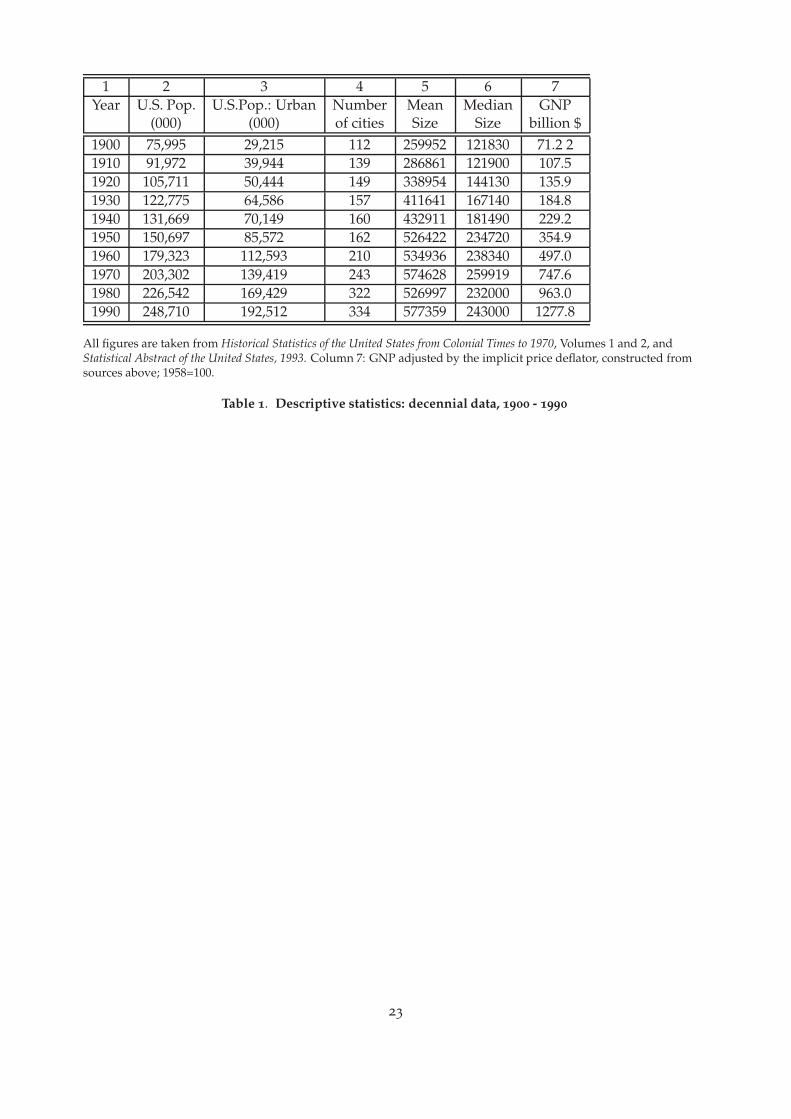
1 2 3 4 5 6 7Year U.S. Pop. U.S.Pop.: Urban Number Mean Median GNP

(000) (000) of cities Size Size billion $1900 75,995 29,215 112 259952 121830 71.2 21910 91,972 39,944 139 286861 121900 107.51920 105,711 50,444 149 338954 144130 135.91930 122,775 64,586 157 411641 167140 184.81940 131,669 70,149 160 432911 181490 229.21950 150,697 85,572 162 526422 234720 354.91960 179,323 112,593 210 534936 238340 497.01970 203,302 139,419 243 574628 259919 747.61980 226,542 169,429 322 526997 232000 963.01990 248,710 192,512 334 577359 243000 1277.8

All figures are taken from Historical Statistics of the United States from Colonial Times to 1970, Volumes 1 and 2, andStatistical Abstract of the United States, 1993. Column 7: GNP adjusted by the implicit price deflator, constructed fromsources above; 1958=100.

Table 1. Descriptive statistics: decennial data, 1900 - 1990

23

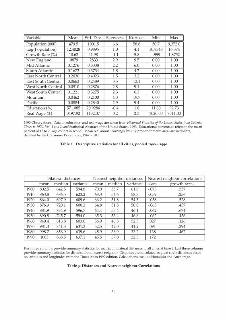
Variable Mean Std. Dev. Skewness Kurtosis Min MaxPopulation (000) 479.5 1001.5 6.6 58.8 50.7 9,372.0Log(Population) 12.4028 0.9895 1.0 4.1 10.8343 16.374Growth Rate (%) 10.62 41.98 -1.1 5.8 -.999 1.8752New England .0879 .2833 2.9 9.5 0.00 1.00Mid Atlantic 0.1276 0.3338 2.2 6.0 0.00 1.00South Atlantic 0.1673 0.3734 1.8 4.2 0.00 1.00East North Central 0.2030 0.4023 1.5 3.2 0.00 1.00East South Central 0.0663 0.2489 3.5 13.1 0.00 1.00West North Central 0.0910 0.2876 2.8 9.1 0.00 1.00West South Central 0.1221 0.3275 2.3 6.3 0.00 1.00Mountain 0.0462 0.2100 4.3 19.7 0.00 1.00Pacific 0.0884 0.2840 2.9 9.4 0.00 1.00Education (%) 57.1085 20.9284 -0.4 1.8 11.80 92.73Real Wage ($) 3197.92 1132.37 0.2 2.3 1020.00 7311.00

1990 Observations. Data on education and real wage are taken from Historical Statistics of the United States from ColonialTimes to 1970, Vol. 1 and 2, and Statistical Abstract of the United States, 1993. Educational percentage refers to the meanpercent of 15 to 20 age cohort in school. Mean real annual earnings, by city proper or metro area, are in dollars,deflated by the Consumer Price Index, 1967 = 100.

Table 2. Descriptive statistics for all cities, pooled 1900 – 1990

Bilateral distances Nearest neighbor distances Nearest neighbor correlationsmean median variance mean median variance sizes growth rates

1900 802.5 642.5 594.8 70.9 55.7 61.8 -.073 .5571910 863.8 686.5 623.2 68.3 54.6 58.3 -.059 .2561920 864.0 697.9 609.6 66.2 51.8 54.5 -.058 .5281930 876.9 720.1 600.2 64.8 51.8 50.0 -.065 .4571940 884.9 734.9 596.7 64.4 53.4 46.1 -.062 .6741950 890.8 745.7 594.0 65.3 53.4 46.6 -.062 .4361960 940.4 813.8 603.0 56.9 46.3 52.5 .027 .1261970 981.3 841.3 631.3 52.5 42.0 41.2 .091 .3941980 998.7 856.9 639.6 45.9 36.9 33.2 .138 .4671990 1005 868.5 637.1 45.5 37.0 32.3 .172

First three columns provide summary statistics for matrix of bilateral distances to all cities at time t. Last three columnsprovide summary statistics for distance from nearest neighbor. Distances are calculated as great circle distances basedon latitudes and longitudes from the Times Atlas 1997 edition. Calculations exclude Honolulu and Anchorage.

Table 3. Distances and Nearest neighbor Correlations

24

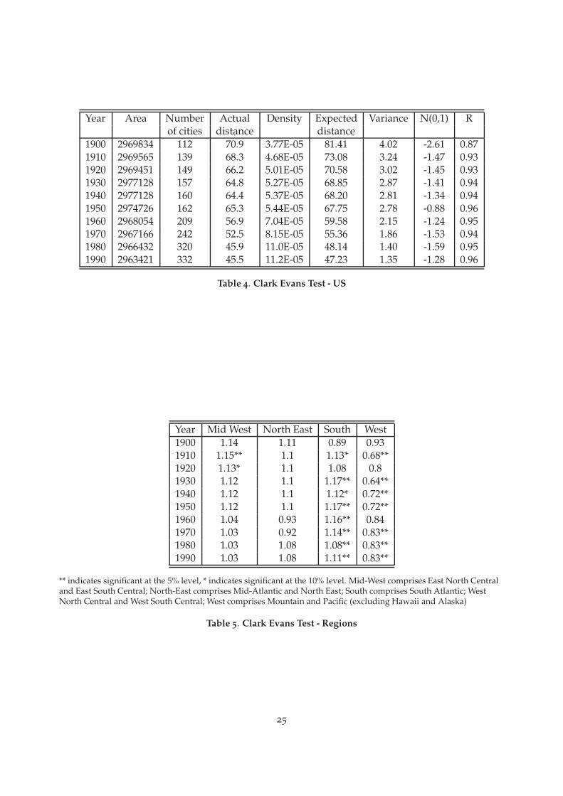
Year Area Number Actual Density Expected Variance N(0,1) Rof cities distance distance

1900 2969834 112 70.9 3.77E-05 81.41 4.02 -2.61 0.871910 2969565 139 68.3 4.68E-05 73.08 3.24 -1.47 0.931920 2969451 149 66.2 5.01E-05 70.58 3.02 -1.45 0.931930 2977128 157 64.8 5.27E-05 68.85 2.87 -1.41 0.941940 2977128 160 64.4 5.37E-05 68.20 2.81 -1.34 0.941950 2974726 162 65.3 5.44E-05 67.75 2.78 -0.88 0.961960 2968054 209 56.9 7.04E-05 59.58 2.15 -1.24 0.951970 2967166 242 52.5 8.15E-05 55.36 1.86 -1.53 0.941980 2966432 320 45.9 11.0E-05 48.14 1.40 -1.59 0.951990 2963421 332 45.5 11.2E-05 47.23 1.35 -1.28 0.96

Table 4. Clark Evans Test - US

Year Mid West North East South West1900 1.14 1.11 0.89 0.931910 1.15** 1.1 1.13* 0.68**1920 1.13* 1.1 1.08 0.81930 1.12 1.1 1.17** 0.64**1940 1.12 1.1 1.12* 0.72**1950 1.12 1.1 1.17** 0.72**1960 1.04 0.93 1.16** 0.841970 1.03 0.92 1.14** 0.83**1980 1.03 1.08 1.08** 0.83**1990 1.03 1.08 1.11** 0.83**

** indicates significant at the 5% level, * indicates significant at the 10% level. Mid-West comprises East North Centraland East South Central; North-East comprises Mid-Atlantic and North East; South comprises South Atlantic; WestNorth Central and West South Central; West comprises Mountain and Pacific (excluding Hawaii and Alaska)

Table 5. Clark Evans Test - Regions

25

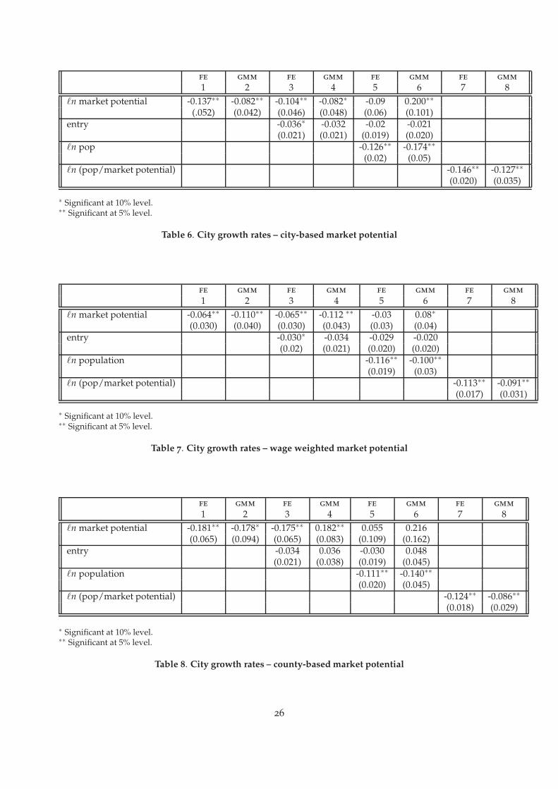
fe gmm fe gmm fe gmm fe gmm1 2 3 4 5 6 7 8

�n market potential -0.137∗∗ -0.082∗∗ -0.104∗∗ -0.082∗ -0.09 0.200∗∗

(.052) (0.042) (0.046) (0.048) (0.06) (0.101)entry -0.036∗ -0.032 -0.02 -0.021

(0.021) (0.021) (0.019) (0.020)�n pop -0.126∗∗ -0.174∗∗

(0.02) (0.05)�n (pop/market potential) -0.146∗∗ -0.127∗∗

(0.020) (0.035)

∗ Significant at 10% level.∗∗ Significant at 5% level.

Table 6. City growth rates – city-based market potential

fe gmm fe gmm fe gmm fe gmm1 2 3 4 5 6 7 8

�n market potential -0.064∗∗ -0.110∗∗ -0.065∗∗ -0.112 ∗∗ -0.03 0.08∗

(0.030) (0.040) (0.030) (0.043) (0.03) (0.04)entry -0.030∗ -0.034 -0.029 -0.020

(0.02) (0.021) (0.020) (0.020)�n population -0.116∗∗ -0.100∗∗

(0.019) (0.03)�n (pop/market potential) -0.113∗∗ -0.091∗∗

(0.017) (0.031)

∗ Significant at 10% level.∗∗ Significant at 5% level.

Table 7. City growth rates – wage weighted market potential

fe gmm fe gmm fe gmm fe gmm1 2 3 4 5 6 7 8

�n market potential -0.181∗∗ -0.178∗ -0.175∗∗ 0.182∗∗ 0.055 0.216(0.065) (0.094) (0.065) (0.083) (0.109) (0.162)

entry -0.034 0.036 -0.030 0.048(0.021) (0.038) (0.019) (0.045)

�n population -0.111∗∗ -0.140∗∗

(0.020) (0.045)�n (pop/market potential) -0.124∗∗ -0.086∗∗

(0.018) (0.029)

∗ Significant at 10% level.∗∗ Significant at 5% level.

Table 8. City growth rates – county-based market potential

26

a: 1910 b: 1910

c: 1990 d: 1990

All calculations done using Danny Quah’s tsrf econometric shell.Stochastic kernel from (normalised) population at time t to (normalised) distance to nearest neighbor at time t.

Figure 1. Population to distance to nearest neighbor

27

a: 1910 b: 1990

All calculations done using Danny Quah’s tsrf econometric shell.Stochastic kernel from (normalised) population at time t to (normalised) date conditioned population at time t.

Figure 2. Date Conditioning

28

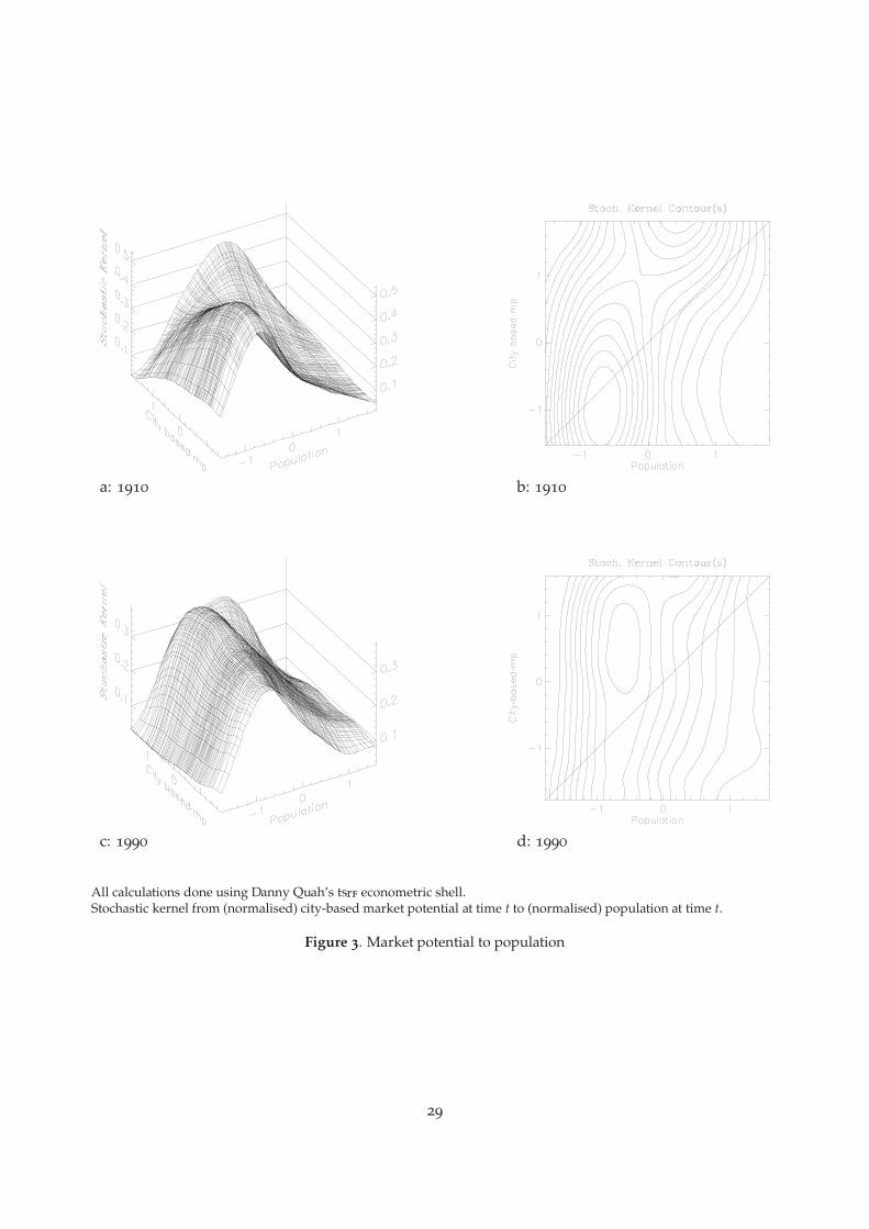
a: 1910 b: 1910

c: 1990 d: 1990

All calculations done using Danny Quah’s tsrf econometric shell.Stochastic kernel from (normalised) city-based market potential at time t to (normalised) population at time t.

Figure 3. Market potential to population

29

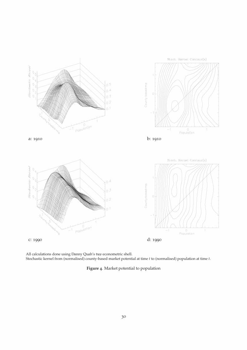
a: 1910 b: 1910

c: 1990 d: 1990

All calculations done using Danny Quah’s tsrf econometric shell.Stochastic kernel from (normalised) county-based market potential at time t to (normalised) population at time t.

Figure 4. Market potential to population

30

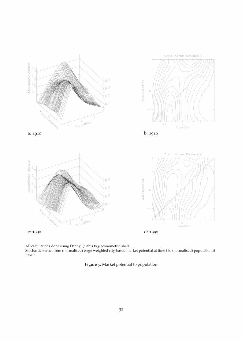
a: 1910 b: 1910

c: 1990 d: 1990

All calculations done using Danny Quah’s tsrf econometric shell.Stochastic kernel from (normalised) wage weighted city-based market potential at time t to (normalised) population attime t.

Figure 5. Market potential to population

31

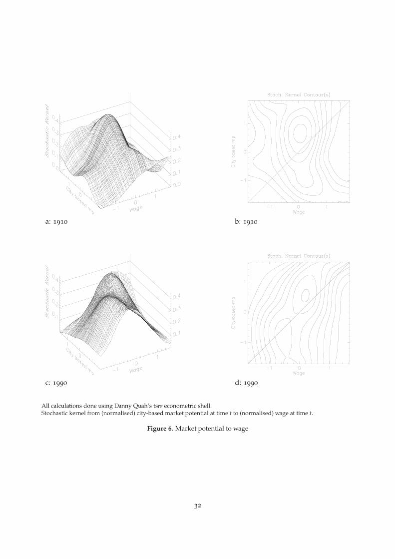
a: 1910 b: 1910

c: 1990 d: 1990

All calculations done using Danny Quah’s tsrf econometric shell.Stochastic kernel from (normalised) city-based market potential at time t to (normalised) wage at time t.

Figure 6. Market potential to wage

32

a: 1910 b: 1990

a: 1910 b: 1990

All calculations done using Danny Quah’s tsrf econometric shell.a & b report stochastic kernels from (normalised) city-based market potential excluding the market potentialcomponent from the nearest neighbor at time t to (normalised) population at time t.c & d report stochastic kernels from (normalised) population at time t to (normalised) population of nearest neighbor attime t.

Figure 7. Nearest neighbor

33

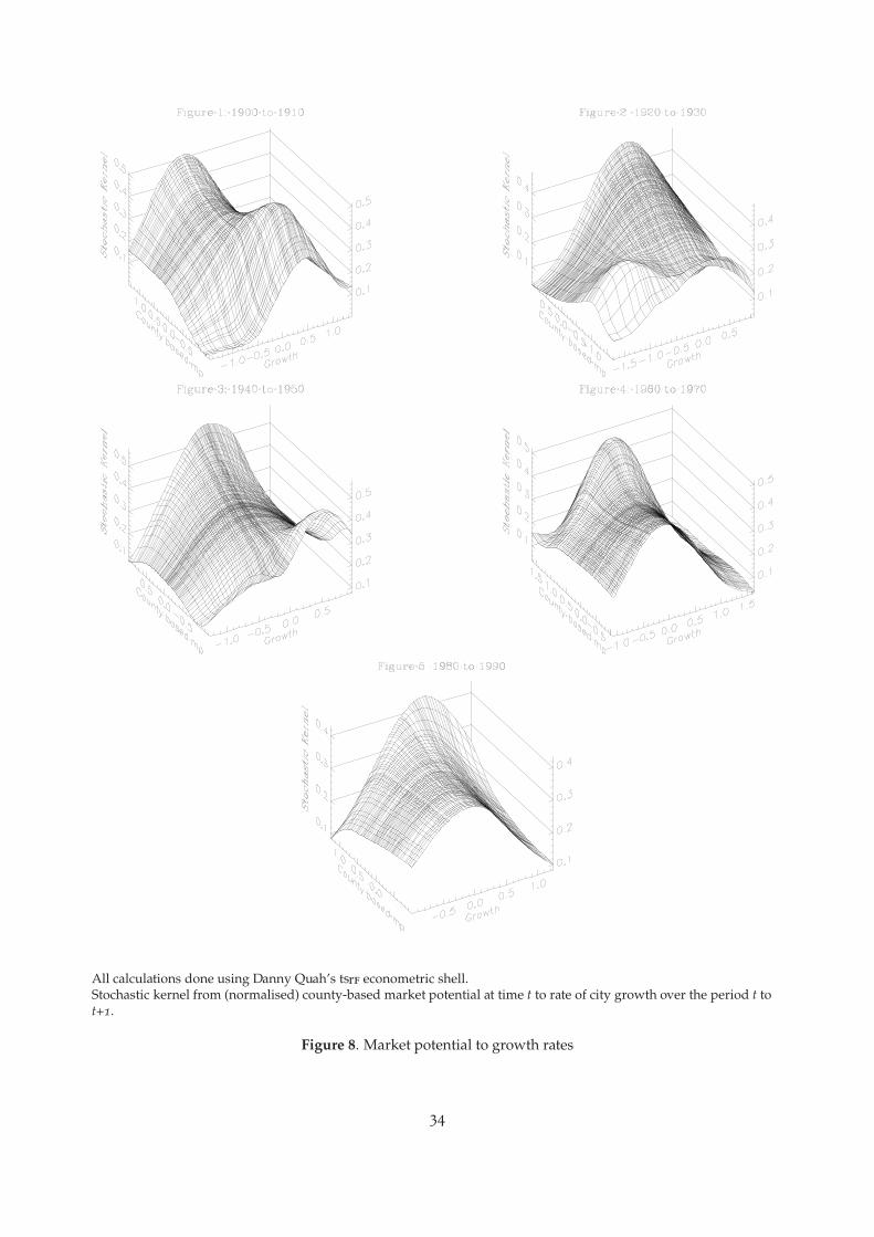
All calculations done using Danny Quah’s tsrf econometric shell.Stochastic kernel from (normalised) county-based market potential at time t to rate of city growth over the period t tot+1.

Figure 8. Market potential to growth rates

34

CENTRE FOR ECONOMIC PERFORMANCE Recent Discussion Papers

481 H. G. Overman Neighbourhood Effects in Small Neighbourhoods

480 S. Gomulka Pension Problems and Reforms in the Czech Republic, Hungary, Poland and Romania

479 S. Nickell T. Jones G. Quintini

A Picture of the Job Insecurity Facing British Men

478 C. Dougherty Numeracy, Literacy and Earnings: Evidence from the National Longitudinal Survey of Youth

477 P. Willman The Viability of Trade Union Organisation: A Bargaining Unit Analysis

476 D. Marsden S. French K. Kubo

Why Does Performance Pay De-Motivate? Financial Incentives versus Performance Appraisal

475 S. Gomulka Macroeconomic Policies and Achievements in Transition Economies, 1989-1999

474 S. Burgess H. Turon

Unemployment Dynamics, Duration and Equilbirum: Evidence from Britain

473 D. Robertson J. Symons

Factor Residuals in SUR Regressions: Estimating Panels Allowing for Cross Sectional Correlation

472 B. Bell S. Nickell G. Quintini

Wage Equations, Wage Curves and All That

471 M. Dabrowski S. Gomulka J. Rostowski

Whence Reform? A Critique of the Stiglitz Perspective

470 B. Petrongolo C. A. Pissarides

Looking Into the Black Box: A Survey of the Matching Function

469 W. H. Buiter Monetary Misconceptions

468 A. S. Litwin Trade Unions and Industrial Injury in Great Britain

467 P. B. Kenen Currency Areas, Policy Domains and the Institutionalization of Fixed Exchange Rates

466 S. Gomulka J. Lane

A Simple Model of the Transformational Recession Under a Limited Mobility Constraint

465 F. Green S. McIntosh

Working on the Chain Gang? An Examination of Rising Effort Levels in Europe in the 1990s

464 J. P. Neary R&D in Developing Countries: What Should Governments Do?

463 M. Güell Employment Protection and Unemployment in an Efficiency Wage Model

462 W. H. Buiter Optimal Currency Areas: Why Does the Exchange Rate Regime Matter?

461 M. Güell Fixed-Term Contracts and Unemployment: An Efficiency Wage Analysis

460 P. Ramezzana Per Capita Income, Demand for Variety, and International Trade: Linder Reconsidered

459 H. Lehmann J. Wadsworth

Tenures that Shook the World: Worker Turnover in Russia, Poland and Britain

458 R. Griffith S. Redding J. Van Reenen

Mapping the Two Faces of R&D: Productivity Growth in a Panel of OECD Industries

457 J. Swaffield Gender, Motivation, Experience and Wages

456 C. Dougherty Impact of Work Experience and Training in the Current and Previous Occupations on Earnings: Micro Evidence from the National Longitudinal Survey of Youth

455 S. Machin Union Decline in Britain

454 D. Marsden Teachers Before the ‘Threshold’

453 H. Gospel G. Lockwood P. Willman

The Right to Know: Disclosure of Information for Collective Bargaining and Joint Consultation

452 D. Metcalf K. Hansen A. Charlwood

Unions and the Sword of Justice: Unions and Pay Systems, Pay Inequality, Pay Discrimination and Low Pay

To order a discussion paper, please contact the Publications Unit

Tel 020 7955 7673 Fax 020 7955 7671 Email info@cep.lse.ac.uk Web site http://cep.lse.ac.uk