Spatial prediction of coral reef habitats: integrating

MARINE ECOLOGY PROGRESS SERIESMar Ecol Prog Ser

Vol. 269: 141–152, 2004 Published March 25

INTRODUCTION

Habitat mapping and community characterization isa prerequisite for condition and resources assessmentof any ecosystem. Improved accuracy and higher reso-lution of output maps are necessary for the optimiza-tion of time and monetary resources invested in fieldresearch. Prediction of habitat distribution is a power-ful tool to help understand ecological processes, andconstitutes a baseline for applied research orientedtowards policy-resource management.

The current applicability and generalization ofremote sensing (RS) research in coral reef habitat map-ping remains problematic due to the intrinsic differ-ences in each studied reef. The choice among severaldata sources available (e.g. Landsat; SPOT — SatellitePour l’Observation de la Terre; Ikonos; CASI —

Compact Airborne Spectrographic Imager), all ofwhich offer different degrees of accuracy, resolutionand spectral characteristics, creates additional dispar-ity. Finally, because of the use of various differenthabitat classification methods and mapping tech-niques, it is difficult to make comparisons betweenapproaches, and this makes each mapping of coral reefhabitats unique (i.e. Mumby et al. 1997, Chauvaud etal. 1998, 1998, Andrefoüet et al. 2000, 2003, Mumby &Edwards 2002, Purkis et al. 2002).

Spatial prediction models are static and probabilis-tic, since they statistically relate the geographical dis-tribution of species or communities to their environ-ment. The quantification of such species-environmentrelationships represents the core of predictive geo-graphical modeling in ecology, and the models arebased on hypotheses of environmental factors control-

© Inter-Research 2004 · www.int-res.com*Corresponding author. Email: [email protected]

Spatial prediction of coral reef habitats: integratingecology with spatial modeling and remote sensing

J. R. Garza-Pérez1, A. Lehmann2, J. E. Arias-González1,*

1Coral Reef Ecosystems Ecology Laboratory, Centro de Investigación y Estudios Avanzados del Instituto Politécnico Nacional Unidad Mérida, Carr. Ant. Progreso km 6 Cordemex, Mérida, Yucatán 97210, México

2Swiss Center for the Cartography of Fauna, Terreaux 14, 2000 Neuchâtel, Switzerland

ABSTRACT: Spatial prediction of coral reef habitats and coral reef community components wasapproached on the basis of the ‘predict first, classify later’ paradigm. Individual community compo-nents (biotic and geomorphologic bottom features) were first predicted and then classified into com-posite habitats. This approach differs from widely applied methods of direct classification based onremote sensing only. In situ coral reef community-condition assessment was first used to measure aresponse variable (percentage cover of habitat). Reef bottom features (topographic complexity, sand-sediment, rock-calcareous pavement and rubble) were then predicted using generalized additivemodels (GAMs) applied to continuous environmental maps, high-resolution Ikonos satellite imagesand a reef digital topographic model (DTM). Next, using GAMs on newly created bottom maps, mod-els were fitted to predict coral community components (hard coral, sea-grass, algae, octocorals). Atthis stage, high-resolution maps of the geomorphologic and biotic components of the coral reef com-munity at an experimental site (Akumal Reef in the Mexican Caribbean) were produced. Coral reefhabitat maps were derived using GIS following a hierarchical classification procedure, and the result-ing merged map depicting 8 habitats was compared against thematic maps created by traditionalsupervised classification. This general approach sets a baseline for future studies involving morecomplex spatial and ecological predictions on coral reefs.

KEY WORDS: GAM · GRASP · GIS · Ikonos · DTM · Mexican Caribbean

Resale or republication not permitted without written consent of the publisher

Mar Ecol Prog Ser 269: 141–152, 2004

ling spatial distribution of species and/or communities(Guisan & Zimmerman 2000).

Spatial prediction modeling has been traditionally aland-based research field (e.g. Leathwick et al. 1998,Tappeiner et al. 1998, 2001, Austin 1999, Debinsky etal. 1999, Bio 2000, Heegard et al. 2001), along with GISapplications for environmental managing (Fedra 1998,Stanbury & Starr 1999, Theobald et al. 2000, Wood-house et al. 2000), with only a few cases applied tomarine resources (e.g. Basu & Nalamotu 1997, Bushing1997). Spatial modeling of underwater communities isslowly being accepted, with recent examples on distrib-ution of submerged vegetation in freshwater ecosys-tems (e.g. Janauer 1997, Lehmann & Lachavanne 1997,Lehmann et al. 1997, Schmieder 1997, Heegard et al.2001, Lehmann 1998) and estuarine fishes distribution(Stoner et al. 2001). More examples can be found in ter-restrial ecosystems (e.g. Münier et al. 2001, Tappeineret al. 2001, Aspinall 2002, Cawsey et al. 2002, Ferrier etal. 2002). All these applications have given rise to thedevelopment of new techniques that incorporategeographic data-base management, spatial modelingand prediction, based on innovative statistical tech-niques such as generalized linear models (GLMs:Chambers & Hastie 1993) and generalized additivemodels (GAMs: Hastie & Tibishirani 1990).

GAMs are non-parametric extensions of GLMs,which originated as a generalization of the classicalleast square relation (LSR) (Yee & Mitchell 1991). Theuse of GAMs has proven to be a very useful tool inecology (Guisan & Zimermann 2000, Austin 2002,Guisan et al. 2002, Lehmann et al. 2002a). Lehmann etal. (2002b) have developed the Generalized Regres-sion Analyses and Spatial Prediction (GRASP) concept,and its implementation encapsu-lates this general approach. WithGRASP, Lehmann et al. (2002a)were able to predict the pre-human distribution of fern biodi-versity in the whole territory ofNew Zealand, by estimating therelationships between fern distrib-utions and the environment, usingsites largely free from human dis-turbance. The main advantage ofthe use of GAMs for this type ofstudy is the ability of the models tofit the data, by estimating theresponse curve with a smoothingfunction (non-parametric). Thisallows the description of environ-mental gradients in better agree-ment with ecological theory, andthe extension of classical regres-sion fitting to other distributions

(binomial, Poisson, gamma) (Hastie & Tibishirani 1990,Yee & Mitchell 1991, Austin 1999, 2002).

The use of these tools (habitat classification, spatialmodelling and remote sensing) is now rapidly growingin coral reef studies. Nevertheless, to our knowledgethis study is the first attempt to apply the GRASPmethodology to predicting habitats in coral reefs. Inthis paper we also apply the paradigm ‘predict first,classify later’ proposed by Overton et al. (2000), incor-porating a modification of the coral reef habitat-classi-fication methodology proposed by González-Gándaraet al. (1999).

MATERIALS AND METHODS

Study area. Akumal Reef is situated in the Northern-Central portion of Quintana Roo State, Mexico, on theeast coast of the Yucatan Peninsula. It is a very welldeveloped fringing reef, with diverse habitats. Coralpatches, sea grass beds and algae prairies can befound in the back reef lagoon. A well-delineated reefcrest, along with calcareous pavement transitionzones, spur and groove systems and sand channels isobserved in the fore reef, down to an approximatedepth of 40 m. We defined the extent of our study areaby a 12 × 1 km strip between 20° 25.995 N, 87° 17.310 Wand 20° 20.005 N to 87° 20.917 W. The reef structurespresent in this area have a relatively homogeneousgeomorphology (Fig. 1). For the definition of the 54sampling stations, we relied on expert knowledge ofthe zone and a high-resolution (4 × 4 m pixel resolu-tion) Ikonos image (Space Imaging), in order to acquirethe geographic coordinates of polygons representing

142

Fig. 1. Study area, Akumal Reef on the coast of Quintana Roo state in Mexico

Garza-Pérez et al.: Spatial prediction of coral reef habitats

different substrata types in all the reef zones (reeflagoon, backreef, crest, fore-reef transition, first stepand second step).

Coral reef community characterization. Characteri-zation and assessment of the benthic communities ateach station was performed using a modified version ofthe Aronson & Swanson (1997) video transect method.We recorded one 50 × 0.6 m transect with a Hi8 Hand-icam (Sony CCDTR-4000) inside an underwater hous-ing (StingRay, Light and Motion). In each transect,temperature (°C), salinity, dissolved oxygen (YSI multi-analyzer, Model 85) and topographic complexity(chain transect) were also recorded. Field work wascompleted with the collaboration of personnel from theCoral Reef Ecosystems Ecology Laboratory at Centrode Investigación y Estudios Avanzados, Merida.

Continuous environmental maps creation. A digitaltopographic model (DTM) was created at 4 × 4 m reso-lution from 6752 echo-sounding and satellite imagedata points, using kriging extrapolation methods inSurfer 8.0 (Golden Software), triangulated irregularnetworks (TIN) and grid functions in 3D analyst exten-sion for ArcGIS 8.1.2 (Environmental SystemsResearch Institute). This DTM was exported toArcView 3.3 (ESRI) for the depth-map query.

The high-resolution Ikonos image (composite image ofblue [B], green [G] and red [R] channels) was treated toobtain a depth invariant index with the method proposedby Green et al. (2000), in order to refine the radiometricand visual information extracted from the image oncethe water column effect was homogenized with it.

The radiometric information of the polygons corre-sponding to the 53 stations in the study area wasextracted from the 4 bands using MultiSpec v.3 soft-ware (for MacOS X, Laboratory for Applications ofRemote Sensing, Purdue University). Each station waspositioned in the image according to the GPS coordi-nates recorded in the field at the start point of eachtransect. During the dives, a compass bearing of eachtransect was recorded, in order to be able to recreatethe area extension of the transects within the satelliteimages (~12 to 15, 4 × 4 m pixels). Another 7 ‘dummy’stations were defined and included, using expertknowledge and the Ikonos image, in order to haveradiometric information on 100% of sand cover and100% sea-grass bed areas.

In order to obtain the spatial predictions of the bioticcomponents of the reef, we needed continuous envi-ronmental maps to correlate the information. Thehigh-resolution satellite images and the bathymetricmap provided an excellent platform for the basic con-tinuous maps. Then 2 consecutive modeling runs wereperformed with GRASP methodology (Lehmann et al.2002a) in S-PLUS 2000 Professional (Insightful) usingbinary and Poisson distributions and exporting the

final predictions as lookup tables (LUTs) to beimported by GRASP scripts in ArcView 3.x (ESRI).GRASP (Lehmann et al. 2002a) is a general method formaking spatial predictions of response variables (RVs)using point surveys of the RVs and spatial coverage ofpredictor variables (PVs). GRASP uses GAMs to fitresponse surfaces as function of predictors in environ-mental space, in order to use the spatial pattern of thepredictor surfaces to predict the response in geo-graphic space. GRASP methodology differs from othergeostatistical analysis (surface-fitting algorithms) inthat it uses surface estimates in ‘predictor space’ andnot directly in ‘geographic space’ (Chambers & Hastie1993, Lehmann et al. 2002a,b,c).

The statistical evaluation of the models was carriedout along with a cross-validation for each selectedmodel, either using correlation coefficient values(Gaussian and Poisson distributions) or receiver operat-ing characteristic (ROC, described in Fielding & Bell1997, for binomial distributions) (Lehmann et al.2002a,b,c). All models were fitted with a quasi-binomialdistribution, using a backwards step-wise procedure toselect the significant predictors, and using the F-statis-tic (p = 0.05) for assessing changes in residual deviance.

GRASP was first used here to predict the geomor-phologic (bottom) features (sand/sediment, rock/cal-careous pavement, rubble and topographic complexity— also known as substratum rugosity) using data fromthe depth map and the 4 satellite image bands as PVs.Topographic complexity and percentage cover of thesubstrata types were used as RVs.

Modeling coral reef’s biotic components withGRASP. Coral reef biotic components were then mod-eled with GRASP as broad functional groups (BFGs).That is percentage cover on the groups: hard corals,octocorals, algae, sea grass and sponges. These werepredicted using percent cover value of each BFG bystations as RVs, and information was derived for sub-strata types, depth, topographic complexity and thedepth corrected satellite image band as PVs.

Coral reef habitat classification. Using data on per-cent cover of BFGs, extracted from the video transects,we proceeded to perform a Monte Carlo test for select-ing the significantly related variables to the structureof our benthic data (CANOCO v.4, Microcomputer-Power), then we used those significant variables toperform an agglomerative cluster analysis using theGower similarity coefficient by Weighted Pair GroupAverage (MVSP v3.12b, Kovach Computing Services);these options were selected because the Gower coeffi-cient is used when mixed data types are present in thematrix, weighted pair group average (WPGMA)because average linking methods provide a more bal-anced approach to clustering, and the weighted optionbecause it was expected that some of the reef habitats

143

Mar Ecol Prog Ser 269: 141–152, 2004

were less sampled than others. In order to correctlyclassify the reef lagoon and the fore-reef habitats, weused 2 separate runs of Monte Carlo tests and 2 clusteranalyses, with the data of the stations corresponding toeither reef lagoon or fore-reef zones. With the obtaineddendrograms, the characteristics of the stations (per-cent coverage of biotic components and substrata,depth, topographic complexity, etc) in each clusterwere averaged in order to obtain the ‘definition’ ofeach cluster (each cluster now treated as a habitat);Note that the ‘cut’ in the dendrogram was not per-fomed at a given similarity (i.e. 75%), but at a distancewhere it ‘made sense’ for each cluster, again, takinginto account expert knowledge of the system. Then adiscriminant analysis (Statistica 6, MathSoft) was per-formed in order to test our ‘hand picked’ (user defined)classification of clusters of stations corresponding toour habitats (also user defined, taking into accountexpert knowledge); since the stations are grouped intodifferent categories (habitats), the test aims to establishthe accuracy of fit of the stations to their categories.

After obtaining the characteristics (percentage ofcover of the different groups, depth, topographic com-plexity, etc) defining each habitat, we performed aquery in the GIS layers (prediction maps) in order to ob-tain habitat distribution maps, which can be displayedover the original high-resolution satellite image.

The implementation of this proposed methodology isdepicted as a flow chart in Fig. 2.

Supervised classification of Ikonos for comparisonwith GRASP. A supervised classification was per-formed on the Ikonos image, usingthe colour bands: blue, green, redand the depth corrected band. Theclassification scheme was definedusing the field stations grouped in thehabitat classification mentionedabove. The classification was repeat-edly performed to redundance byseveral decision rules, minimum dis-tance (or spectral distance) being theone selected for this analysis.

RESULTS

Digital topographic model (DTM)

The DTM layer imported toArcView was rasterized at the sameresolution as the original DTMmodel (4 × 4 m pixel resolution) anda continuous depth map (0 to –35 m)of the study area was extracted(Fig. 3).

144

Fig. 3. Akumal digital topographic model (DTM) from echo-sounding survey,Ikonos high-resolution satellite image overlay on top of the DTM and raster

extraction (0 to 35 m depth) from ‘depth’ layer in the GIS

Fig. 2. Workflow of the proposed implementation of coral-reef-habitat spatial prediction. The hexagon is the naturalsystem, rounded rectangles are information collected by di-verse methods, ellipsoids are data treatments and rectanglesare outputs/results. GRASP: Generalized Regression Ana-

lyses and Spatial Prediction


Satellite image enhancement

A linearization of the light absorption in the satelliteimage was performed with combinations of bands of theimage (B-G, G-R, B-R). Applying the algebraic transfor-mation to the band combinations (with MultiSpec v.3software), we obtained new channels and decided to useB-R because it offered a better definition of the bottomfeatures than the other 2 combinations (Fig. 4).

Spatial prediction

With the first run of GRASPmodeling (validation, V, andcross-validation, CV, values ofthe models, ranging from 0.7 to 1ROC), we obtained the predictionand prediction standard error(pSE) maps of topographic com-plexity (TC) values, rock/calcare-ous pavement, sand/sedimentand rubble cover (Fig. 5), all witha spatial definition of 4 × 4 m pix-els. An actual sand/sediment pSEmap was included in the figure toillustrate this feature in the analy-sis.

For the second GRASP run, the model correlation values (V and CV) ranged from 68.3 to86.2% for hard corals, octocoralsand calcareous-articulated algae.

Green algae and brown/filamentous algae modelsshowed ROC values (V and CV) of 0.6 and 0.8, respec-tively. The prediction and pSE maps of the biotic com-ponents of the reef were obtained, also at 4 × 4 m reso-lution; see Fig. 6, where the brown/filamentous algaepSE map was included in order to illustrate this featurein the analysis.

A separate modeling run was performed for predic-tion of seagrasses, in a separate set of layers, queriedto display only the reef lagoon areas of the studyzone (Fig. 6). The evaluation and cross-validation ofthe model by ROC statistic was 0.94 (see Table 1 for

145

Fig. 4. Satellite band combinations with algebraic transformation, for water-column effect correction (small excerpt from thewhole treated image to show better detail). (a) blue and green (B-G), (b) green and red (G-R), and (c) blue and red (B-R) band

combinations (this last combination provided the best correction)

Fig. 5. Base maps (reef geomorphologic features) predicted with GRASP: (a) rubble,(b) rock/calcareous pavement, (c) topographic complexity, (d) sand/sediment, (e) sand/sediment prediction standard error (pSE). Gradient values given as % cover except

(c) and (e)

Mar Ecol Prog Ser 269: 141–152, 2004

initial and final models, degrees offreedom used in the smoothing,validation and cross-validationvalues).

Habitat classification

The Monte Carlo tests showed 7significant variables (p < 0.05) outof 14 (hard coral, octocoral, brown/filamentous algae, calcareous/articulated algae, green algae,recent dead coral and sponges), forclassifying the fore-reef (slope)habitats, and 7 out of 14 for classify-ing the reef lagoon (sea grass,brown/filamentous algae, hard

146

Fig. 6. GRASP of biotic components coverage: (a) seagrass (reef lagoon area extrac-tion), (b) hard corals, (c) octocorals, (d) calcareous-articulated algae, (e) green algae,(f) brown/filamentous algae, (g) brown/filamentous algae prediction standard error

(pSE). Gradient values given as % cover, except (g)

Table 1. Initial (all predictive variables included) and final (selected predictive variables) GAMs for geomorphologic and bioticresponse variables, as produced by GRASP interface, where s = spline smoother; names in parentheses are the variables intro-duced in the models: bands 1, 2, 3 and 4, correspond to satellite image bands red, green, blue and water column depth correctedcomposite; depth = depth; sand = sand/sediment; rock = rock/calcareous pavement; rubble = rubble; ct = topographic complexity;and values after comma are degrees of freedom of the spline smoother. ROC: receiver operating characteristic; COR: correlation.Example: Response Variable: s(Predictive Variable1, degrees of freedom for the spline smoother)+ s(Predictive Variable2, degrees

of freedom for the spline smoother)+...

Variable Initial model Final model Validation Cross-Validation

Rock/ Rock: s(band1,4) Rock: s(band1,4) ROC:0.7 ROC:0.7calcareous +s(band2,4)+s(band3,4) +s(B1,3Comp,4)pavement +s(B1,3Comp,4)+s(depth,4)

Sand/ Sand: s(band1,4)+s(band2,4) Sand: s(band1,4)+s(band2,1) ROC:0.875 ROC:0.875sediment +s(band3,4)+s(band4,4) +s(band4,4)+s(depth,4)

+s(depth,4)

Rubble Rubble: s(band1,4)+s(band2,4) Rubble: s(band1,4) ROC:0.798 ROC:0.798+s(band3,4)+s(band4,4) +s(band2,1)+s(band4,4+s(depth,4) +s(depth,1)

Topographic TopogComp.: s(band1,3) Topog.Comp.: s(band1,3) ROC: 1.0 ROC: 1.0complexity +s(band2,3)+ s(band3,3) +s(band4,3)

+s(band4,3)+ s(depth,3)

Hard coral HardCoral: s(band1,4) HardCoral: s(band1,1) COR:0.862 COR:0.778+s(band2,4)+ s(band3,4) +s(band3,1)+s(band4,1)+s(band4,4)+ s(depth,4)+ s(ct,4) +s(depth,4)+ s(sand,4)+s(rubble,4)+ s(rock,4)+s(sand,4)

Octocoral Octocoral: s(band4,4)+s(depth,4) Octocoral: s(band4,1) COR:0.840 COR:0.771+s(ct,4)+s(rubble,4)+s(rock,4) +s(ct,1)+ s(rock,4)+s(sand,1)+s(sand,4)

Green algae GreenAlgae: s(band4,4) GreenAlgae: s(band4,1) ROC:0.606 ROC:0.606+s(depth,4)+ s(ct,4)+ s(rubble,4) +s(depth,1)+ s(sand,4)+s(rock,4)+s(sand,4)

Filamentous/ Filam.Brwn.Algae: s(band4,4) Filam.Brwn.Algae: ROC: 0.8 ROC: 0.8brown algae +s(depth,4)+ s(ct,4)+ s(rubble,4) s(rock,4)+ s(sand,4)

+s(rock,4)+s(sand, 4)

Calcareous Calc.Artic.Algae: s(band,4) Calc.Arctic.Algae: s(depth,4) COR:0.683 COR:0.564articulated algae +s(depth,4)+ s(ct,4)+ s(rubble,4) +s(sand,1)

+s(rock,4)+s(sand,4)

Seagrass SG: s(band1,4)+ s(band2,4) SG: s(band2,4) ROC: 0.941 ROC: 0.941+s(band3,4)+ s(band4,4)+s(depth,4)+s(rubble,4)+s(Sand,4)+s(ct,4)+s(Rock,4)


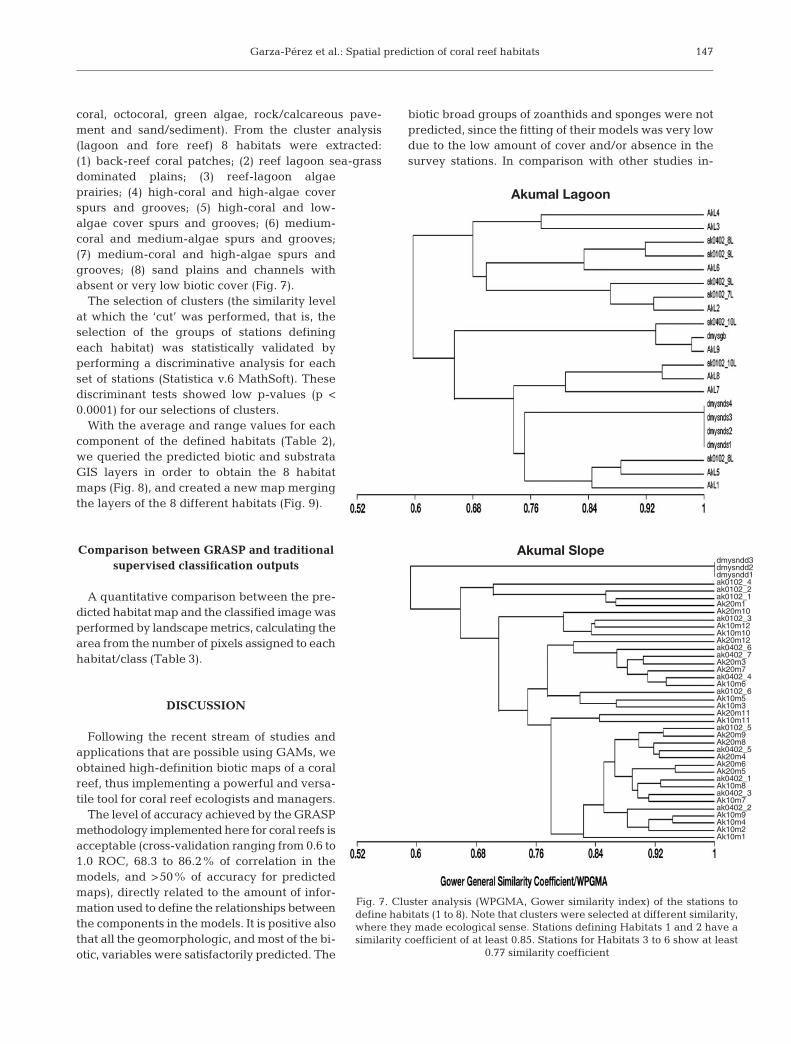
coral, octocoral, green algae, rock/calcareous pave-ment and sand/sediment). From the cluster analysis(lagoon and fore reef) 8 habitats were extracted:(1) back-reef coral patches; (2) reef lagoon sea-grassdominated plains; (3) reef-lagoon algaeprairies; (4) high-coral and high-algae coverspurs and grooves; (5) high-coral and low-algae cover spurs and grooves; (6) medium-coral and medium-algae spurs and grooves;(7) medium-coral and high-algae spurs andgrooves; (8) sand plains and channels withabsent or very low biotic cover (Fig. 7).

The selection of clusters (the similarity levelat which the ‘cut’ was performed, that is, theselection of the groups of stations definingeach habitat) was statistically validated byperforming a discriminative analysis for eachset of stations (Statistica v.6 MathSoft). Thesediscriminant tests showed low p-values (p <0.0001) for our selections of clusters.

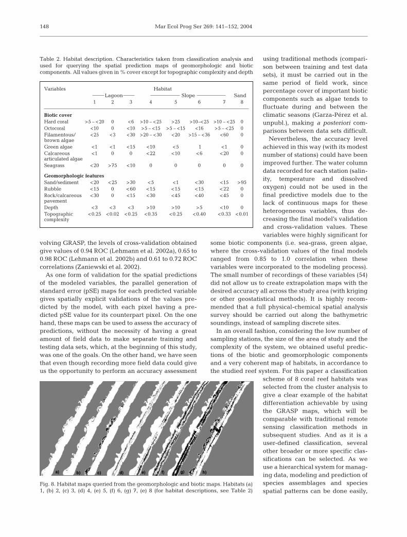
With the average and range values for eachcomponent of the defined habitats (Table 2),we queried the predicted biotic and substrataGIS layers in order to obtain the 8 habitatmaps (Fig. 8), and created a new map mergingthe layers of the 8 different habitats (Fig. 9).

Comparison between GRASP and traditionalsupervised classification outputs

A quantitative comparison between the pre-dicted habitat map and the classified image wasperformed by landscape metrics, calculating thearea from the number of pixels assigned to eachhabitat/class (Table 3).

DISCUSSION

Following the recent stream of studies andapplications that are possible using GAMs, weobtained high-definition biotic maps of a coralreef, thus implementing a powerful and versa-tile tool for coral reef ecologists and managers.

The level of accuracy achieved by the GRASPmethodology implemented here for coral reefs isacceptable (cross-validation ranging from 0.6 to1.0 ROC, 68.3 to 86.2% of correlation in themodels, and >50% of accuracy for predictedmaps), directly related to the amount of infor-mation used to define the relationships betweenthe components in the models. It is positive alsothat all the geomorphologic, and most of the bi-otic, variables were satisfactorily predicted. The

biotic broad groups of zoanthids and sponges were notpredicted, since the fitting of their models was very lowdue to the low amount of cover and/or absence in thesurvey stations. In comparison with other studies in-

147

Fig. 7. Cluster analysis (WPGMA, Gower similarity index) of the stations todefine habitats (1 to 8). Note that clusters were selected at different similarity,where they made ecological sense. Stations defining Habitats 1 and 2 have asimilarity coefficient of at least 0.85. Stations for Habitats 3 to 6 show at least

0.77 similarity coefficient

dmysndd3dmysndd2dmysndd1ak0102_4ak0102_2ak0102_1Ak20m1Ak20m10ak0102_3Ak10m12Ak10m10Ak20m12ak0402_6ak0402_7Ak20m3Ak20m7ak0402_4Ak10m6ak0102_6Ak10m5Ak10m3Ak20m11Ak10m11ak0102_5Ak20m9Ak20m8ak0402_5Ak20m4Ak20m6Ak20m5ak0402_1Ak10m8ak0402_3Ak10m7ak0402_2Ak10m9Ak10m4Ak10m2Ak10m1

Akumal Lagoon

Akumal Slope

Mar Ecol Prog Ser 269: 141–152, 2004

volving GRASP, the levels of cross-validation obtainedgive values of 0.94 ROC (Lehmann et al. 2002a), 0.65 to0.98 ROC (Lehmann et al. 2002b) and 0.61 to 0.72 ROCcorrelations (Zaniewski et al. 2002).

As one form of validation for the spatial predictionsof the modeled variables, the parallel generation ofstandard error (pSE) maps for each predicted variablegives spatially explicit validations of the values pre-dicted by the model, with each pixel having a pre-dicted pSE value for its counterpart pixel. On the onehand, these maps can be used to assess the accuracy ofpredictions, without the necessity of having a greatamount of field data to make separate training andtesting data sets, which, at the beginning of this study,was one of the goals. On the other hand, we have seenthat even though recording more field data could giveus the opportunity to perform an accuracy assessment

using traditional methods (compari-son between training and test datasets), it must be carried out in thesame period of field work, sincepercentage cover of important bioticcomponents such as algae tends tofluctuate during and between theclimatic seasons (Garza-Pérez et al.unpubl.), making a posteriori com-parisons between data sets difficult.

Nevertheless, the accuracy levelachieved in this way (with its modestnumber of stations) could have beenimproved further. The water columndata recorded for each station (salin-ity, temperature and dissolvedoxygen) could not be used in thefinal predictive models due to thelack of continuous maps for theseheterogeneous variables, thus de-creasing the final model’s validationand cross-validation values. Thesevariables were highly significant for

some biotic components (i.e. sea-grass, green algae,where the cross-validation values of the final modelsranged from 0.85 to 1.0 correlation when thesevariables were incorporated to the modeling process).The small number of recordings of these variables (54)did not allow us to create extrapolation maps with thedesired accuracy all across the study area (with krigingor other geostatistical methods). It is highly recom-mended that a full physical-chemical spatial analysissurvey should be carried out along the bathymetricsoundings, instead of sampling discrete sites.

In an overall fashion, considering the low number ofsampling stations, the size of the area of study and thecomplexity of the system, we obtained useful predic-tions of the biotic and geomorphologic componentsand a very coherent map of habitats, in accordance tothe studied reef system. For this paper a classification

scheme of 8 coral reef habitats wasselected from the cluster analysis togive a clear example of the habitatdifferentiation achievable by usingthe GRASP maps, which will becomparable with traditional remotesensing classification methods insubsequent studies. And as it is auser-defined classification, severalother broader or more specific clas-sifications can be selected. As weuse a hierarchical system for manag-ing data, modeling and prediction ofspecies assemblages and speciesspatial patterns can be done easily,

148

Fig. 8. Habitat maps queried from the geomorphologic and biotic maps. Habitats (a)1, (b) 2, (c) 3, (d) 4, (e) 5, (f) 6, (g) 7, (e) 8 (for habitat descriptions, see Table 2)

Table 2. Habitat description. Characteristics taken from classification analysis andused for querying the spatial prediction maps of geomorphologic and biotic components. All values given in % cover except for topographic complexity and depth

Variables HabitatLagoon Slope Sand

1 2 3 4 5 6 7 8

Biotic coverHard coral >5 – <20 0 <6 >10 – <25 >25 >10–<25 >10 – <25 0Octocoral <10 0 <10 >5 – <15 >5 – <15 <16 >5 – <25 0Filamentous/ <25 <3 <30 >20 – <30 <20 >15 – <36 <60 0brown algaeGreen algae <1 <1 <15 <10 <5 1 <1 0Calcareous <1 0 0 <22 <10 <6 <20 0articulated algaeSeagrass <20 >75 <10 0 0 0 0 0

Geomorphologic featuresSand/sediment <20 <25 >30 <5 <1 <30 <15 >95Rubble <15 0 <60 <15 <15 <15 <22 0Rock/calcareous <30 0 <15 <30 <45 <40 <45 0pavementDepth <3 <3 <3 >10 >10 >5 <10 0Topographic <0.25 <0.02 <0.25 <0.35 <0.25 <0.40 <0.33 <0.01complexity


thus giving ecological robustness tothe characterization of the system.

The comparison between GRASPand traditional supervised classifica-tion outputs using the same imageand classification scheme provided,in a sense, another validation of theGRASP maps. The classificationscheme of 8 classes was selected, tak-ing into account the results of An-drefoüet et al. (2003), to evaluate coralreef areas with Ikonos images. The 8-class thematic map produced with thesupervised classification methodologydid not show an accurate spatial defi-nition of classes (see Fig. 9), as it wasunable to separate Habitat 4 fromHabitat 6 (see Table 2 for habitat de-scription), so a new classification wasperformed, this time with 9 classes(Fig. 9), separating shallow sand fromdeep sand stations. The new thematicmap was more in accordance with theGRASP map, assigning most classesinto similar spatial distribution pat-terns; nevertheless the GRASP mapprovided an image more in accor-dance with reality. The traditional su-pervised classification method pre-sented a spatial incorrect estimationof habitats, thus affecting the inter-pretability and usefulness of the clas-sified map, and had less spatial accu-racy when delimiting boundaries ofclasses (Table 3, Fig. 9). This is proba-bly due to the minimum-distance de-cision rule used, which tends to clas-sify pixels that otherwise should gounclassified, and does not considerclass variability (ERDAS 1999). Thisdecision rule provided the best interpretation of ourclassification scheme and fitted more appropriately toour data set. The GRASP-derived (habitat) map pre-sents ‘unclassified’ areas corresponding to geomorpho-logic features and biotic component coverage valuesnot represented in the field data and thus not taken intoaccount in the habitat definition (from the classifica-tion). However, the GRASP maps of individual featuresand components include wider predicted ranges of val-ues, below and above those registered in the field, inorder to depict the gradients of coverage all along thestudy area. Thus GRASP turned out to be more robustfor producing predictive maps, validating the method-ology proposed here for obtaining useful spatial predic-tions over large areas from small datasets.

Expert knowledge of a system, along with the use ofhigh-resolution satellite images, plays a very importantrole in this kind of research. In this study this helped us,for instance, to establish a focused sampling design in or-der to record the greatest amount of possible variation inthe coral reef habitats with the least cost.

Other studies, using GAMs for prediction of vegeta-tion distribution in terrestrial ecosystems (Yee &Mitchell 1991, Leathwick et al. 1998, Lehmann &Austin 1999, Cawsey et al. 2002, Ferrier et al. 2002Lehmann et al. 2002a,b) in New Zealand and Aus-tralia, have achieved very good results in the fittingand stability of the models and in the accuracy of pre-dictions, using spatial resolutions ranging from 1 × 1to 5 × 5 km, regardless of the great areas involved

149

Fig. 9. Classified map of Akumal Coral Reef: (a) whole study area map showing the8 habitats (h1 to h8) queried from the geomorphologic and biotic maps obtained bygeneralized regression analyses and spatial prediction (GRASP) methodology,(b) close-up view of a small portion to enhance details of the habitat mapping byGRASP, (c) view of the same zoomed area of the Ikonos image treated by super-vised classification (minimum distance), following an 8-class scheme, (d) same por-tion and procedure as in (c), but following a 9-class scheme (including h9)

Mar Ecol Prog Ser 269: 141–152, 2004

(New South Wales and New Zealand territories). Oneof the factors involved in the fitting and accuracy ofthese models is the great amount of data used (setsranging in the thousands of plots), which areextracted from sources such as national vegetationand forest surveys. Unfortunately these data sets arealmost non-existent or not reliable in most third-worldcoral reef areas, and our implementation offers a goodalternative for characterization and condition assess-ment.

The direct ecological applications for these GRASPcontinuous maps on coral reefs are: (1) reef habitat as-sessment, which allows us to identify hot spots of bioticfeatures, (2) use as baseline information to classify andcharacterize the spatial extent of each defined habitat,(3) helping in management tasks (defining zones withinmarine reserves, defining the probable distribution andabundance of any given resource), (4) characterization ofthe spatial relationships between coral reef fish benthiccommunities (Arias-Gonzalez et al. unpubl.).

One key utility of this implementation of spatial pre-diction in coral reefs is that from a relatively small areawe are able to scale up the predictions to greater areasin the Mexican Caribbean fringing reef system, andthe methodology (though not the models) can be easilytransported to other reef areas in the world.

Currently we are applying this methodology to sea-plain atoll-type reefs in the Caribbean Sea (ChinchorroBank [Gulf of Mexico] and Alacranes Reef) and theGreat Barrier Reef (Davies Reef) (Acosta-González etal. unpubl., Arias-González et al. unpubl.).

In contrast with common remote-sensing classifica-tion procedures (non-supervised and supervised clas-sification), in this methodology we do not assign eachpixel to individual classes (thus our expression ofhard-classification, where a pixel can belong to oneclass only per image treatment), but each pixel has a

value assigned to each different layer,giving us the possibility to map thesubtle variations of the components ofthe reef as a continuum. The a posteri-ori merging and classification of thecontinuous maps into habitats hasmore to do with the human need tobreak things into smaller comprehen-sive portions. As Townsend (2000)points out, the delineation of classes onmaps is necessary to facilitate the com-munication of information about spatialpatterns of the distribution and abun-dance of species.

In the technical aspect of this study,Ikonos high-resolution satellite imag-ery has proven to be more useful forpredictive tasks (such as this GRASP

application) than for ‘hard’ classification by remotesensing procedures. In a recent study, Andrefoüet etal. (2003) stated that for management and scientificapplications that need at least 80% of accuracy, only a4- to 5-class scheme can be used with Ikonos imagery,and that hard coral cover areas are poorly classifiedmost of the time, especially when these areas alsoinclude algae coverage. In this case we have beenable to obtain spatial predicted coverage values ofeach one of the most important biotic components(including corals and 3 different types of algae) andgeomorphologic characteristics of our study area,thus giving a wider range of uses and applications forthe spatial information obtained. Ikonos imagery isreferred to as not very effective in cost-benefit termsin comparison with Landsat TM for coarse-level habi-tat mapping, but its value in defining boundaries ofhabitat patches over other types of imagery is recog-nized (Mumby & Edwards 2002). This favorable char-acteristic allows the use of expert knowledge in orderto implement and refine a directed sampling efforttowards recording the maximum possible variation inthe system.

In order to establish the advantages (or not) of theimplementation of this methodology in coral reefecosystems, we are currently comparing the results ofGRASP against traditional ‘hard classification’ meth-ods (relying only on spectral information) for mappingcoral-reef biotic and geomorphologic features, usingIkonos and Landsat 7 ETM+ imagery (for 3 reefs in theMexican Caribbean). We are also investigating thefeasibility of extending the spatial predictions to largerreef areas using Landsat 7 ETM+ images of the north-ern part of Quintana Roo state in Mexico. The presentstudy can be taken as the introduction of GRASP tocoral reef ecology; the comparison between methodswould be a second step towards full validation of the

150

Table 3. Landscape metrics. Area estimated for each habitat from GRASP habi-tat map, and from supervised classification image (8- and 9-class scheme). Allvalues expressed in m2. All habitats correspond to description in Table 2, exceptin the 9-class scheme, where former Habitat 8 was divided into shallow and

deep sand

Habitat GRASP 8-class scheme 9-class scheme

1 117 552 391216 6897922 217 696 560496 5249123 1137 936 1044 496 2299044 704 128 603424 6034245 1096 608 853808 8538086 705 104 4424592 35518247 2564 544 3033008 30330088 2868 240 1374288 11538409 – – 1644816

Total 9411 808 12285328 12285328Total study area 12285328 12285328 12285328


GRASP application and implementation on coral reefsystems.

Partial approaches to our methodology are pro-posed by Mumby & Harbone (1999), who propose ahierarchical classification scheme for the Caribbeanreefs; by Andrefouët & Claereboudt (2000), who use aclassification scheme of coral reefs that correlates theenvironmental data with remotely sensed data (SPOT-HRV); by Aspinall (2002), who used logistic regressionto validate vegetation maps extracted from a high-definition hyperspectral airborne scanner (128 bands,ESSI Probe 1); by Guisan & Zimmermann (2000) intheir review of predictive habitat-distribution model-ing; by Overton et al. (2002) in proposing a pyramidalstructure of data management; and by Ferrier et al.(2002) who propose a similar implementation and useof community-level modeling with GAMs in terrestrialecosystems. In this study we merged several pro-posals from other science fields to implement thismethodology in coral reef ecology.

As pointed out by Yee & Mitchell (1991) severalyears ago, and recently by Lehmann et al. (2002a),GAMs and GRASP are computer tools that demandhigh processor performance and large memory capac-ity when used over large areas at high resolution (sev-eral million pixels). Using GRASP in coral reef areasat high resolution (4 m), as we did in this exercise, ispossible since the extension of reef area is restrictedto a narrow zone in the satellite image. For applica-tions over greater reef areas such as bank reefs, i.e.Alacran Reef in the Gulf of Mexico (Arias-Gonzalez etal. unpubl.) and Chinchorro Bank in the CaribbeanSea, the option could be the use of Landsat 7 ETM+imagery (30 × 30 m pixel resolution), since coveringsuch areas with Ikonos imagery would be very costly.Nevertheless, if money for such investment (imageryand computers) is not a main constraint, the comput-ing power of the latest generation of processors andcurrent memory capacity has reached the point wherethe size of the data files is becoming less important.

As a conclusion, we can state that the methodologyimplemented here, incorporating habitat charac-terization and topology, 3D topographic models,remote sensing techniques, and spatial prediction(GRASP) in coral reefs, is an effective, useful and reli-able way to map extensive coral reef areas with a rela-tively small investment in field surveys. Combiningthis GRASP application with time series of communityassessment in selected stations on the reef, we couldimplement a forecast of reef condition and analyzechanges of its components over time. As this methodol-ogy is fully compatible with GIS, new layers of relatedinformation could be added as they become available,and they may improve the prediction accuracy and sta-bility of our initial models.

Acknowledgements. We would like to thank CONACyT inMexico for funding this research (proyecto #28386 N, becacredito 119328 and beca crédito mixta para estancias en elextranjero), also to thank the kind help and support of theSwiss Center for the Fauna Cartography (CSCF, Neuchâtel)for the first stage of this project. This study would not havebeen possible without the timely collaboration of S.Andrefoüet and F. Muller-Karger at the Remote Sensing Lab-oratory, USF St. Petersburg, and NASA data-buy program foracquiring the Ikonos imagery. Thanks to the Akumal DiveShop (D. Brewer, G. Arcila and crew) and Akumal CEA, for allthe kind support in field activities. Also to the Coral ReefEcosystems Ecology Lab members (LEEAC Adventure Team),for their valuable time and help in field activities. We wouldalso like to thank to P. J. Mumby for his valuable comments onthe original manuscript and the kind observations and com-ments from 4 anonymous referees.

LITERATURE CITED

Andrefouët S, Claereboudt M (2000) Objective class defini-tion using correlation of similartities between remotelysensed and environmental data. Int J Rem Sens 21(9):1925–1930

Andrefouët S, Roux L, Chancerelle Y, Boneville A (2000) Afuzzy probabilistic scheme of study for objects with indeter-minate boundaries: application to French Polynesian reefs-capes. IEEE Transactions on Geosci Rem Sens 38(1):257–270

Andrefouët S, Kramer P, Torres-Pulliza D, Joyce KE and 10others (2003) Multi-sites evaluation of Ikonos data for clas-sification of tropical coral reef environments. Rem SensEnviron 88:128–143.

Aronson RB, Swanson DW (1997) Video surveys of coral reefs:uni and multivariate applications. Proc 8th Int Coral ReefSymp 2:1923–1926

Aspinall RJ (2002) Use of logistic regression for validation ofmaps of the spatial distribution of vegetation speciesderived from high spatial resolution hyperspectralremotely sensed data. Ecol Model 157:301–312

Austin MP (1999) The potential contribution of vegetationecology to biodiversity research. Ecography 22:465–484

Austin MP (2002) Spatial prediction of species distribution: aninterface between ecological theory and statistical model-ling. Ecol Model 157(2):101–118

Basu A, Nalamotu C (1997) Marine geographic informationsystem for the exclusive economic zone. Mar Geod 20(2-3):255–266

Bio AMF (2000) Does vegetation suit our models? Data andmodel assumptions and the assessment of species distrib-ution in space. PhD thesis, Utretch University

Bushing WW (1997) GIS-based gap analysis of an existingmarine reserve network around Santa Catalina island.Mar Geod 20(2-3):205–234

Cawsey EM, Austin MP, Baker BL (2002) Regional vegetationmapping in Australia: a case study in the practical use ofstatistical modelling. Biodiversity Conserv 11:2239–2274

Chavaud S, Bouchon C, Marniere R (1998) Remote sensingtechniques adapted to high resolution mapping of tropicalcoastal marine ecosystems (coral reefs, seagrass beds andmangrove). Int J Rem Sens 19(18):3625–3639

Chambers EM, Hastie TJ (1993) Statistical models. Chapmanand Hall, London

Debinski DM, Kindscher K, Jakubaukas ME (1999) A remotesensing and GIS-based model of habitats and biodiversityin the Greater Yellowstone Ecosystem. Int J Rem Sens 20(17):3281–3291

151

Mar Ecol Prog Ser 269: 141–152, 2004

ERDAS (1999) Field guide, 5th edn. ERDAS, AtlantaFedra K (1998) Geographic information systems and spatial

analysis in coastal zone management. Mar Ind Technol1,2: 1–12

Ferrier S, Drielsma M, Manion G, Watson G (2002) Extendedstatistical approaches to modelling spatial pattern in bio-diversity in north-east New South Wales: II. Communitylevel modelling. Biodiversity Conserv 11:2309–2338

Fielding AH, Bell JF (1997) A review of methods for theassessment of predictions errors in conservation pres-ence/absence models. Environmental Conserv 24(1):38–49

González-Gándara C, Membrillo-Venegas N, Nuñez-Lara E,Arias-González JE (1999) The relationship between fishand reefscapes in the Alacranes Reef, Yucatan, Mexico: apreliminary trophic functioning analysis. Vie Milieu 49(4):275–286

Green EP, Mumby PJ, Alasdair JE, Clark CD (2000) Remotesensing handbook for tropical coastal management.UNESCO, Paris

Guisan A, Zimmerman NE (2000) Predictive habitat distribu-tion models in ecology. Ecol Model 135 147–186

Guisan A, Edwards TC, Hastie T (2002) Generalized linearand generalized additive models in studies of species dis-tributions: setting the scene. Ecol Model 157(2–3)89–100

Hastie T, Tibishirani R (1990) Generalized additive models.Chapman Hall, London

Heegaard E, Birks HH, Gibson CE, Smith SJ, Wolfe-MurphyS (2001) Species-environmental relationships of aquaticmacrophytes in Northern Ireland. Aquat Bot 70 175–223

Janauer GA (1997) Macrophytes, hydrology, and aquatic eco-tones: a GIS-supported ecological survey. Aquat Bot 58:379–391

Leathwick JR, Burns BR, Clarkson BD (1998) Environmentalcorrelates of three alpha-divesity in New Zealand primaryforests. Ecography 21:235–246

Lehmann A (1998) GIS modelling of submerged macrophytedistribution using generalized additive models. Plant Ecol139:113–124

Lehmann A, Austin M (1999) Implementing GRASP to predicttree distribution in Southeastern NSW and to test differentpotential measures of water stress. Report to the Divisionof Wildlife and Ecology, CSIRO, Canberra

Lehmann A, Lachavanne JB (1997) Geographic informationsystems and remote sensing in aquatic botany. Aquat Bot58:195–207

Lehmann A, Jaquet JM, Lachavanne JB (1997) A GISapproach of aquatic plant spatial heterogeneity in relationto sediment and depth gradients, Lake Geneva, Switzer-land. Aquat Bot 58:347–361

Lehmann A, Overton JMC, Leathwick JR (2002a) GRASP:Generalized Regression Analysis and Spatial Predictions.Ecol Model 157:189–207

Lehmann A, Leathwick, JR, Overton J McC (2002b) AssessingNew Zealand fern diversity from spatial predictions ofspecies assemblages. Biodiversity Conserv 11:2217–2238

Lehmann AJ, Overton, M, Austin MP (2002c) Regressionmodels for spatial prediction: their role for biodiversityand conservation. Biodivesity Conserv 11:2085–2092

Mumby PJ, Edwards AJ (2002) Mapping marine environ-ments with Ikonos imagery: enhanced spatial resolutioncan deliver greater thematic accuracy. Rem Sens Environ82:248–257

Mumby PJ, Harborne AR (1999) Development of a systematicclassification scheme of marine habitats to facilitateregional management and mapping of Caribbean coralreefs. Biological Conserv 88:155–163

Mumby PJ, Green EP, Edwards AJ, Clark CD (1997) Coralreef habitat-mapping: how much detail can remote sens-ing provide? Mar Biol 130:193–202

Mumby PJ, Green EP, Clark CD, Edwards AJ (1998) Digitalanalysis of multispectral airborne imagery of coral reefs.Coral Reefs 17:59–69

Münier B, Nygaard B, Ejrnæs, Bruun HG (2001) A biotopelandscape model for prediction of semi-natural vegetationin Denmark. Ecol Model 139:221–233

Overton JM, Leathwick JR, Lehmann A (2000) Predict first,classify later – a new paradigm of spatial classification forenvironmental management: a revolution in the mappingof vegatation, soil, land cover and other environmentalinformation. 4th Int Conf Integrating GIS and Environ-mental Modelling: Problems, Prospects and ResearchNeeds. Banff, Alberta. Available at www.colorado.edu/research/cires/banff/pubpapers/212/

Overton JM, Stephens RTT, Leathwick JR, Lehmann A (2002)Information pyramids for informed biodiversity conserva-tion. Biodiversity Conserv 11:2093–2116

Purkis S, Kenter JAM, Oikononomu E, Robinson IS (2002)High resolution ground verification, cluster analysis andoptical model of reef substrate coverage on Landsat TMimagery (Red Sea, Egypt). Int J of Rem Sens 23:1677–1698

Schmieder K (1997) Littoral zone-GIS of Lake Constance: auseful tool in lake monitoring and autecological studieswith submersed macrophytes. Aquat Bot 58:333–346

Stanbury KB, Starr RM (1999) Applications of geographicinformation systems (GIS) to habitat assessment andmarine resource management. Oceanol Acta 22 (6):699–703

Stoner AW, Manderson JP, Pessutti JP (2001) Spatially explicitanalysis of estuarine habitat for juvenile winter flounder:combining generalized additive models and geographicinformation systems. Mar Ecol Prog Ser 213:253–271

Tappeiner U, Tasser E, Tappeiner G (1998) Modelling vegeta-tion patterns using natural and anthropogenic influencefactors: preliminary experience with a GIS based modelapplied to an alpine area. Ecol Model 113:225–237

Tappeiner U, Tappeiner G, Aschenwald J, Tasser E, Osten-dorf B (2001) GIS based modelling of spatial pattern ofsnow cover duration in an alpine area. Ecol Model 138:265–275

Theobald DM, Hobbs NT, Bearly T, Zack JA Shenk T, Rieb-same WE (2000) Incorporating biological information inlocal land-use decision making: designing a system forconservation planning. Landscape Ecol 15:35–45

Townsend PA (2000) A quantitative fuzzy approach to assessmapped vegetation classifications for ecological applica-tions. Rem Sens Environ 72:253–267

Woodhouse S, Lovett A, Dolman, P, Fuller R (2000) Using aGIS to select priority areas for conservation. Computers,Environment Urban Syst 24:79–93

Yee TW, Mitchell ND (1991) Generalized additive models inplant ecology. J Veg Sci 2:587–602

Zaniewski AE, Lehmann A, Overton JMcC (2002) Predictingspecies distribution using presence-only data: a case studyof native New Zealand fern. Ecol Model 157:261–280

152

Editorial responsibility: Otto Kinne (Editor), Oldendorf/Luhe, Germany

Submitted: July 16, 2003; Accepted: December 31, 2003Proofs received from author(s): March 15, 2004

Documents

Spatial prediction of coral reef habitats: integrating