Embed Size (px)
Citation preview
Spatiotemporal Multiplier Networks for Video Action Recognition
Christoph Feichtenhofer *
Graz University of Technology
Axel Pinz
Graz University of Technology
Richard P. Wildes
York University, Toronto
Abstract
This paper presents a general ConvNet architecture for
video action recognition based on multiplicative interac-
tions of spacetime features. Our model combines the ap-
pearance and motion pathways of a two-stream architec-
ture by motion gating and is trained end-to-end. We theo-
retically motivate multiplicative gating functions for resid-
ual networks and empirically study their effect on classi-
fication accuracy. To capture long-term dependencies we
inject identity mapping kernels for learning temporal rela-
tionships. Our architecture is fully convolutional in space-
time and able to evaluate a video in a single forward pass.
Empirical investigation reveals that our model produces
state-of-the-art results on two standard action recognition
datasets.
1. Introduction
Extremely deep representations have recently been
highly successful in numerous pattern recognition compe-
titions. Residual Networks (ResNets) [11] provide a struc-
tural concept for easing the training of deep architectures
by inserting skip-connections for direct propagation of gra-
dients from the loss layer at the end of the network to
early layers close to the input. Recently, spatiotemporal
ResNets (ST-ResNets) [8] have been presented as a com-
bination of two-stream networks [28] with ResNets. The
resulting architecture nontrivially extended the performance
of the original two-stream approach in application to action
recognition on standard datasets.
While the ST-ResNet [8] yielded state-of-the-art perfor-
mance in application to action recognition, it did not pro-
vide systematic justification for its design choices. Our cur-
rent work reconsiders the combination of the two-stream
and ResNet approaches in a more thorough fashion to in-
crease the understanding of how these techniques interact,
*Christoph Feichtenhofer is a recipient of a DOC Fellowship of the
Austrian Academy of Sciences at the Institute of Electrical Measurement
and Measurement Signal Processing, Graz University of Technology.
Appearance Stream
Motion Stream
∙∙ ∙
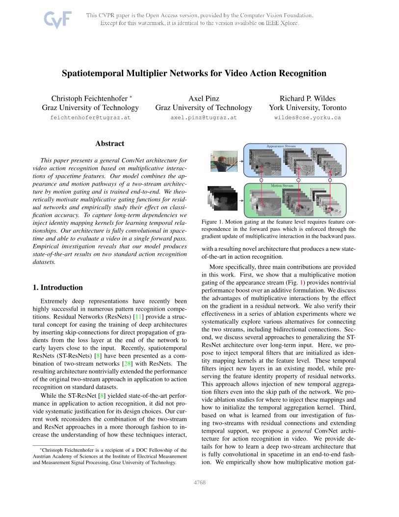
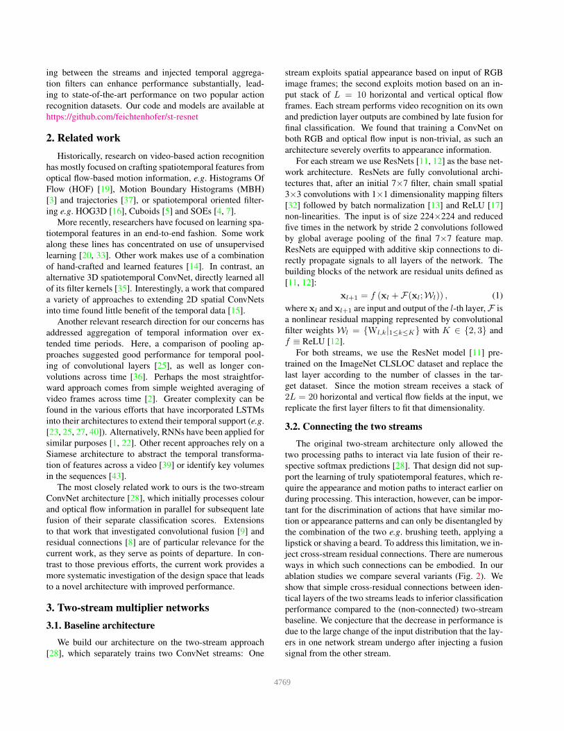
Figure 1. Motion gating at the feature level requires feature cor-
respondence in the forward pass which is enforced through the
gradient update of multiplicative interaction in the backward pass.
with a resulting novel architecture that produces a new state-
of-the-art in action recognition.
More specifically, three main contributions are provided
in this work. First, we show that a multiplicative motion
gating of the appearance stream (Fig. 1) provides nontrivial
performance boost over an additive formulation. We discuss
the advantages of multiplicative interactions by the effect
on the gradient in a residual network. We also verify their
effectiveness in a series of ablation experiments where we
systematically explore various alternatives for connecting
the two streams, including bidirectional connections. Sec-
ond, we discuss several approaches to generalizing the ST-
ResNet architecture over long-term input. Here, we pro-
pose to inject temporal filters that are initialized as iden-
tity mapping kernels at the feature level. These temporal
filters inject new layers in an existing model, while pre-
serving the feature identity property of residual networks.
This approach allows injection of new temporal aggrega-
tion filters even into the skip path of the network. We pro-
vide ablation studies for where to inject these mappings and
how to initialize the temporal aggregation kernel. Third,
based on what is learned from our investigation of fus-
ing two-streams with residual connections and extending
temporal support, we propose a general ConvNet archi-
tecture for action recognition in video. We provide de-
tails for how to learn a deep two-stream architecture that
is fully convolutional in spacetime in an end-to-end fash-
ion. We empirically show how multiplicative motion gat-
14768
ing between the streams and injected temporal aggrega-
tion filters can enhance performance substantially, lead-
ing to state-of-the-art performance on two popular action
recognition datasets. Our code and models are available at
https://github.com/feichtenhofer/st-resnet
2. Related work
Historically, research on video-based action recognition
has mostly focused on crafting spatiotemporal features from
optical flow-based motion information, e.g. Histograms Of
Flow (HOF) [19], Motion Boundary Histograms (MBH)
[3] and trajectories [37], or spatiotemporal oriented filter-
ing e.g. HOG3D [16], Cuboids [5] and SOEs [4, 7].
More recently, researchers have focused on learning spa-
tiotemporal features in an end-to-end fashion. Some work
along these lines has concentrated on use of unsupervised
learning [20, 33]. Other work makes use of a combination
of hand-crafted and learned features [14]. In contrast, an
alternative 3D spatiotemporal ConvNet, directly learned all
of its filter kernels [35]. Interestingly, a work that compared
a variety of approaches to extending 2D spatial ConvNets
into time found little benefit of the temporal data [15].
Another relevant research direction for our concerns has
addressed aggregation of temporal information over ex-
tended time periods. Here, a comparison of pooling ap-
proaches suggested good performance for temporal pool-
ing of convolutional layers [25], as well as longer con-
volutions across time [36]. Perhaps the most straightfor-
ward approach comes from simple weighted averaging of
video frames across time [2]. Greater complexity can be
found in the various efforts that have incorporated LSTMs
into their architectures to extend their temporal support (e.g.
[23, 25, 27, 40]). Alternatively, RNNs have been applied for
similar purposes [1, 22]. Other recent approaches rely on a
Siamese architecture to abstract the temporal transforma-
tion of features across a video [39] or identify key volumes
in the sequences [43].
The most closely related work to ours is the two-stream
ConvNet architecture [28], which initially processes colour
and optical flow information in parallel for subsequent late
fusion of their separate classification scores. Extensions
to that work that investigated convolutional fusion [9] and
residual connections [8] are of particular relevance for the
current work, as they serve as points of departure. In con-
trast to those previous efforts, the current work provides a
more systematic investigation of the design space that leads
to a novel architecture with improved performance.
3. Two-stream multiplier networks
3.1. Baseline architecture
We build our architecture on the two-stream approach
[28], which separately trains two ConvNet streams: One
stream exploits spatial appearance based on input of RGB
image frames; the second exploits motion based on an in-
put stack of L = 10 horizontal and vertical optical flow
frames. Each stream performs video recognition on its own
and prediction layer outputs are combined by late fusion for
final classification. We found that training a ConvNet on
both RGB and optical flow input is non-trivial, as such an
architecture severely overfits to appearance information.
For each stream we use ResNets [11, 12] as the base net-
work architecture. ResNets are fully convolutional archi-
tectures that, after an initial 7×7 filter, chain small spatial
3×3 convolutions with 1×1 dimensionality mapping filters
[32] followed by batch normalization [13] and ReLU [17]
non-linearities. The input is of size 224×224 and reduced
five times in the network by stride 2 convolutions followed
by global average pooling of the final 7×7 feature map.
ResNets are equipped with additive skip connections to di-
rectly propagate signals to all layers of the network. The
building blocks of the network are residual units defined as
[11, 12]:
xl+1 = f (xl + F(xl;Wl)) , (1)
where xl and xl+1 are input and output of the l-th layer,F is
a nonlinear residual mapping represented by convolutional
filter weights Wl = {Wl,k|1≤k≤K} with K ∈ {2, 3} and
f ≡ ReLU [12].
For both streams, we use the ResNet model [11] pre-
trained on the ImageNet CLSLOC dataset and replace the
last layer according to the number of classes in the tar-
get dataset. Since the motion stream receives a stack of
2L = 20 horizontal and vertical flow fields at the input, we
replicate the first layer filters to fit that dimensionality.
3.2. Connecting the two streams
The original two-stream architecture only allowed the
two processing paths to interact via late fusion of their re-
spective softmax predictions [28]. That design did not sup-
port the learning of truly spatiotemporal features, which re-
quire the appearance and motion paths to interact earlier on
during processing. This interaction, however, can be impor-
tant for the discrimination of actions that have similar mo-
tion or appearance patterns and can only be disentangled by
the combination of the two e.g. brushing teeth, applying a
lipstick or shaving a beard. To address this limitation, we in-
ject cross-stream residual connections. There are numerous
ways in which such connections can be embodied. In our
ablation studies we compare several variants (Fig. 2). We
show that simple cross-residual connections between iden-
tical layers of the two streams leads to inferior classification
performance compared to the (non-connected) two-stream
baseline. We conjecture that the decrease in performance is
due to the large change of the input distribution that the lay-
ers in one network stream undergo after injecting a fusion
signal from the other stream.
4769
+
conv
conv
+
conv
conv
+
conv
conv
+
conv
conv
Motion
Stream
Appearance
Stream
ReLU
ReLU
ReLU
ReLU
ReLU
ReLU
ReLU
(a)
+
conv
conv
+
conv
conv
+
conv
conv
+
conv
conv
Motion
Stream
Appearance
Stream
ReLU
ReLU
ReLU
ReLU
ReLU
ReLU
ReLU
ReLU
∙
(b)
+
conv
conv
+
conv
conv
+
conv
conv
+
conv
conv
Motion
Stream
Appearance
Stream
+ReLU
ReLU
ReLU
ReLU
ReLU
ReLU
ReLU
(c)
+
conv
conv
+
conv
conv
+
conv
conv
+
conv
conv
Motion
Stream
Appearance
Stream
ReLU
ReLU
ReLU
ReLU
ReLU
ReLU
ReLU
∙
(d)
+
conv
conv
+
conv
conv
+
conv
conv
+
conv
conv
Motion
Stream
Appearance
Stream
ReLU
ReLU
ReLU
ReLU
ReLU
ReLU
Motion &
Appearance
Gating ∙∙
(e)
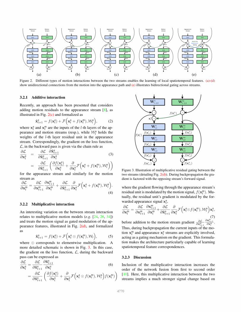
Figure 2. Different types of motion interactions between the two streams enables the learning of local spatiotemporal features. (a)-(d)
show unidirectional connections from the motion into the appearance path and (e) illustrates bidirectional gating across streams.
3.2.1 Additive interaction
Recently, an approach has been presented that considers
adding motion residuals to the appearance stream [8], as
illustrated in Fig. 2(c) and formalized as
xal+1 = f(xa
l) + F(
xal + f(xm
l ),Wal
)
, (2)
where xal and x
ml are the inputs of the l-th layers of the ap-
pearance and motion streams (resp.), while Wal holds the
weights of the l-th layer residual unit in the appearance
stream. Correspondingly, the gradient on the loss function,
L, in the backward pass is given via the chain rule as
∂L
∂xal
=∂L
∂xal+1
∂xal+1
∂xal
(3)
=∂L
∂xal+1
(
∂f(xal)
∂xal
+∂
∂xal
F(
xal + f(xm
l ),Wal
)
)
for the appearance stream and similarly for the motion
stream as∂L
∂xml
=∂L
∂xml+1
∂xml+1
∂xml
+∂L
∂xal+1
∂
∂xal
F(
xal + f(xm
l ),Wal
)
.
(4)
3.2.2 Multiplicative interaction
An interesting variation on the between stream interaction
relates to multiplicative motion models (e.g. [24, 26, 34])
and treats the motion signal as gated modulation of the ap-
pearance features, illustrated in Fig. 2(d), and formalized
as
xal+1 = f(xa
l) + F(
xal ⊙ f(xm
l ),Wl
)
, (5)
where ⊙ corresponds to elementwise multiplication. A
more detailed schematic is shown in Fig. 3. In this case,
the gradient on the loss function, L, during the backward
pass can be expressed as
∂L
∂xal
=∂L
∂xal+1
∂xal+1
∂xal
(6)
=∂L
∂xal+1
(
∂f(xal)
∂xal
+∂
∂xal
F(
xal ⊙ f(xm
l ),Wal
)
f(xml )
)
+
+
+
+
)( alf x
a3,1lW
a1,lW
a2,lW
a3,lW
)( a1lf x
)( a1,lf x
)( a2,lf x
)( a3,lf x
m3,1lW
m1,lW
m2,lW
m3,lW
)( mlf x
)( m1lf x
)( m1,lf x
)( m2,lf x
)( m3,lf x
alx ∙
Figure 3. Illustration of multiplicative residual gating between the
two streams (detailing Fig. 2(d)). During backpropagation the gra-
dient is factored with the opposing stream’s forward signal.
where the gradient flowing through the appearance stream’s
residual unit is modulated by the motion signal, f(xml ). Mu-
tually, the residual unit’s gradient is modulated by the for-
warded appearance signal xal ,
∂L
∂xml
=∂L
∂xml+1
∂xml+1
∂xml
+∂L
∂xal+1
∂
∂xal
F(
xal⊙f(x
ml ),W
al
)
xal ,
(7)
before addition to the motion stream gradient ∂L∂xm
l+1
∂xml+1
∂xml
.
Thus, during backpropagation the current inputs of the mo-
tion xml and appearance x
al streams are explicitly involved,
acting as a gating mechanism on the gradient. This formula-
tion makes the architecture particularly capable of learning
spatiotemporal feature correspondences.
3.2.3 Discussion
Inclusion of the multiplicative interaction increases the
order of the network fusion from first to second order
[10]. Here, this multiplicative interaction between the two
streams implies a much stronger signal change based on
4770
spatiotemporal feature correspondence compared to the ad-
ditive interaction (2): In the former case, (5), the mo-
tion information directly scales the appearance information
through the term xal ⊙ f(xm
l ), rather than via a more sub-
tle bias, xal + f(xm
l ), as in the additive case, (2). Dur-
ing backpropagation, instead of the fusion gradient flow-
ing through the appearance, (3), and motion, (4), streams
being distributed uniformly due to additive forward inter-
action (2), it now is multiplicatively scaled by the oppos-
ing stream’s current inputs, f(xml ) and x
al in equations (6)
and (7), respectively. This latter type of interaction allows
the streams to more effectively interact during the learning
process and corresponding spatiotemporal features thereby
ultimately are captured (cf. similar discussion in the context
of recurrent networks [41]).
Finally, rather than asymmetrically injecting the motion
information into the appearance stream, bidirectional con-
nections could be employed. Such processing could be re-
alized for either additive or multiplicative interactions and
is illustrated for the multiplicative case in Fig. 2(e). In em-
pirical evaluation, we show that such interactions yield infe-
rior performance to the asymmetric case of injecting motion
into appearance. We conjecture that this result comes about
because the spatial stream comes to dominate the motion
stream during training.
3.3. Temporal filtering with feature identity
Beyond very limited means for interaction between its
processing paths, the original two-stream network also em-
ployed only a small temporal window (10 frames) in mak-
ing its predictions, which subsequently were averaged over
the video [28]. In contrast, many real world actions required
larger intervals of time to be defined unambiguously (e.g.
consider a “lay-up” in basketball). Thus, the second way
that we improve on the two-stream architecture is to provide
it with greater temporal support (cf. [8, 9, 36] for previous
work with similar motivations).
We employ 1D temporal convolutions combined with
feature space transformations initialized as identity map-
pings to achieve our goal. 1D convolutions provide a
learning-efficient way to capture temporal dependencies,
e.g. with far less overhead than LSTMs. Initialization of
the feature transformations as identity mappings is appro-
priate when injecting into deep architectures, as any sig-
nificant change in the network path would distort the (pre-
trained) model and thereby remove most of its representa-
tional power. Furthermore, preserving the feature identity
is essential to preserve the design principles of residual net-
works. The corresponding kernels can be injected at any
point in the network since they do not impact the informa-
tion flow at initialization; however, during training they can
adapt their representation under the gradient flow.
Formally, we inject temporal convolutional layers into
+
+
)33(2, lW
)11(1, lW
)11(3, lW
)11(3,1 lW
)311(
lW
(a) †
+
+
)33(2, lW
)11(1, lW
)11(3, lW
)11(3,1 lW
)311(
lW
(b) ‡, §
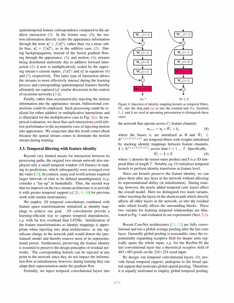
Figure 4. Injection of identity mapping kernels as temporal filters,
Wl, into the skip path (a) or into the residual unit (b). Symbols
†, ‡ and § are used in upcoming presentation to distinguish these
cases.
the network that operate across Cl feature channels
xl+1 = xl ∗ Wl + bl, (8)
where the biases bl are initialized as 0 and Wl ∈R
1×1×T×Cl×Cl are temporal filters with weights initialized
by stacking identity mappings between feature channels,
1 ∈ R1×1×1×Cl×Cl , across time t = 1 . . . T . Specifically,
Wl = 1⊗ f , (9)
where⊗ denotes the tensor outer product and f is a 1D tem-
poral filter of length T . Notably, eq. (9) initializes temporal
kernels to perform identity transforms at feature level.
Since our kernels preserve the feature identity, we can
place them after any layer in the network without affecting
its representational ability (at initialization). During train-
ing, however, the newly added temporal conv layers affect
the overall model. Here we distinguish two main variants,
either inserting the layers in the shortcut path which directly
affects all other layers in the network, or into the residual
units which locally affects the surrounding blocks. These
two variants for learning temporal relationships are illus-
trated in Fig. 4 and evaluated in our experiments (Sect. 5.2).
Recent ConvNet architectures [11, 31] are fully convo-
lutional and use a global average pooling after the last conv
layer. Generally global pooling is reasonable, since the ex-
ponentially expanding receptive field for deeper units typ-
ically spans the whole input, e.g. for the ResNet-50 the
last convolutional layer has a theoretical receptive field of
483×483 pixels on the 224×224 sized input.
By design, our temporal convolutional layers, (8), pro-
vide broad temporal support, analogous to the broad spa-
tial support that motivates global spatial pooling. Therefore,
it is equally motivated to employ global temporal pooling.
4771
Layers conv1 pool1 conv2 x conv3 x conv4 x conv5 x pool5
Blocks7×
7, 64
3×3
max
1×1, 643×3, 641×1, 256
1×1, 1283×3, 1281×1, 512
1×1, 2563×3, 256
1×1, 1024
1×1, 5123×3, 5121×1, 2048
7×7
avgstride 2
⊙ ⊙ ⊙ ⊙
1×1, 643×3, 64 ‡1×1, 256
1×1, 1283×3, 128 ‡1×1, 512
1×1, 2563×3, 256 ‡1×1, 1024
1×1, 5123×3, 512 ‡, §
1×1, 2048
1×1, 643×3, 641×1, 256
1×1, 1283×3, 1281×1, 512
×N
1×1, 2563×3, 256
1×1, 1024
×M
1×1, 5123×3, 5121×1, 2048
† † † †
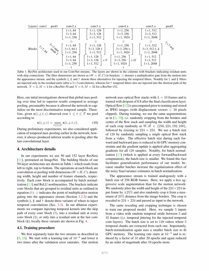
Table 1. ResNet architecture used in our ConvNet streams. The layers are shown in the columns with brackets indicating residual units
with skip connections. The filter dimensions are shown as (W ×H,C) in brackets. ⊙ denotes a multiplicative gate from the motion into
the appearance stream, and the symbols ‡, § and † denote three alternatives for injecting the temporal filters. Notably for ‡ and § filters
are injected only in the residual units (after a 3×3 convolution), whereas for † temporal filters also are injected into the shortcut path of the
network. N = 2, M = 4 for a ResNet-50 and N = 6,M = 32 for a ResNet-152.
Here, our intial investigations showed that global max pool-
ing over time led to superior results compared to average
pooling, presumably because it allowed the network to cap-
italize on the most discriminative temporal sample. There-
fore, given x(i, j, t, c) observed over 1 ≤ t ≤ T we pool
according to
x(i, j, c) = max1≤t≤T
x(i, j, t, c). (10)
During preliminary experiments, we also considered appli-
cation of temporal max-pooling earlier in the network; how-
ever, it always produced inferior results to pooling after the
last convolutional layer.
4. Architecture details
In our experiments we use 50 and 152 layer ResNets
[11], pretrained on ImageNet. The building blocks of our
50-layer architecture are shown in Table 1 which reads from
left to right, top to bottom. The operations at each block are
convolution or pooling with dimensions (W×H,C), denot-
ing width, height and number of feature channels, respec-
tively. Each conv block is accompanied by batch normal-
ization [13] and ReLU nonlinearities. The brackets indicate
conv blocks that are grouped to residual units as outlined in
equation (1). ⊙ indicates the point of multiplicative motion
gating into the appearance stream (Section 3.2.2) and the
symbols ‡, § and † denote three variants of where to inject
temporal convolutions (Sec. 3.3). In our ablation experi-
ments we compare injecting temporal kernels into the skip
path of every conv block (†), into a residual unit at every
conv block (‡), or only into a residual unit at the last conv
block (§); locally these variants are shown in Fig. 4.
4.1. Training procedure
We first separately train the two streams as described in
[9, 28]. We start with a learning rate of 10−2 and lower it
two times after the validation error saturates. Our motion
network uses optical flow stacks with L = 10 frames and is
trained with dropout of 0.8 after the final classification layer.
Optical flow [42] is precomputed prior to training and stored
as JPEG images (with displacement vectors > 20 pixels
clipped). During training, we use the same augmentations
as in [1, 39]; i.e. randomly cropping from the borders and
centre of the flow stack and sampling the width and height
of each crop randomly as W,H ∈ {256, 224, 192, 168},followed by resizing to 224 × 224. We use a batch size
of 128 by randomly sampling a single optical flow stack
from a video. The effective batch size during each for-
ward and backward pass is reduced to fit GPU memory con-
straints and the gradient update is applied after aggregating
gradients for all 128 samples. Notably, for batch normal-
ization [13] (which is applied at every forward/backward
computation), the batch-size is smaller. We found this fact
facilitates generalization performance of our model, be-
cause smaller batches increase the regularization effect of
the noisy bias/variance estimates in batch normalization.
The appearance stream is trained analogously with a
batch size of 256 RGB frames. Here, we apply a less ag-
gressive scale augmentation than for the motion network:
We randomly jitter the width and height of the 224×224 in-
put frame by ±25% and also randomly crop it from a max-
imum of 25% distance from the image borders. The crop is
rescaled to 224× 224 and passed as input to the network.
The same rescaling and cropping technique is chosen
to train our proposed model. Here, we sample 5 inputs
from a video with random temporal stride between 5 and
35 frames (i.e. temporal jittering for the injected temporal
conv-layers). The batch size is set to 128 videos where 5temporal chunks are extracted from each one. Importantly,
batch-normalization again uses a smaller batch size to fit
GPU memory. The learning rate starts at 10−3 and is re-
duced by a factor of 10 after 20 epochs and again reduced
by an order of magnitude after 10 epochs more.
4772
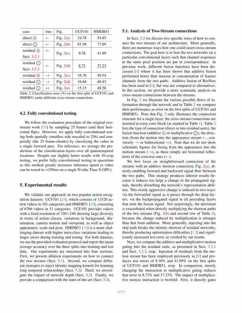
case into Fig. UCF101 HMDB51
direct +© ← Fig. 2(a) 24.78 54.85
direct⊙
← Fig. 2(b) 81.98 77.89
residual +© ←Fig. 2(c) 9.38 41.89
Sect. 3.2.1
residual⊙
← Fig. 2(d) 8.72 37.23Sect. 3.2.2
residual +© → Fig. 2(c) 16.76 49.54
residual⊙
→ Fig. 2(d) 16.68 48.43
residual⊙
↔ Fig. 2(e) 15.15 48.56
Table 2. Classification error (%) on the first split of UCF101 and
HMDB51 under different cross-stream connections.
4.2. Fully convolutional testing
We follow the evaluation procedure of the original two-
stream work [28] by sampling 25 frames (and their hori-
zontal flips). However, we apply fully convolutional test-
ing both spatially (smallest side rescaled to 256) and tem-
porally (the 25 frame-chunks) by classifying the video in
a single forward pass. For inference, we average the pre-
dictions of the classification layers over all spatiotemporal
locations. Despite our slightly better results with 10-crop
testing, we prefer fully convolutional testing in spacetime
as this method greatly increases inference speed (a video
can be tested in ≈250ms on a single Nvidia Titan X GPU).
5. Experimental results
We validate our approach on two popular action recog-
nition datasets: UCF101 [29], which consists of 13320 ac-
tion videos in 101 categories and HMDB51 [18], consisting
of 6766 videos in 51 categories. UCF101 provides videos
with a fixed resolution of 320×240 showing large diversity
in terms of action classes, variations in background, illu-
mination, camera motion and viewpoint, as well as object
appearance, scale and pose. HMDB51 [18] is a more chal-
lenging dateset with higher intra-class variations leading to
larger errors during training and testing. For both datasets,
we use the provided evaluation protocol and report the mean
average accuracy over the three splits into training and test
data. Our experiments are structured into four sections.
First, we present ablation experiments on how to connect
the two streams (Sect. 5.1). Second, we compare differ-
ent strategies to inject identity mapping kernels for learning
long temporal relationships (Sect. 5.2). Third, we investi-
gate the impact of network depth (Sect. 5.3). Finally, we
provide a comparison with the state-of-the-art (Sect. 5.4).
5.1. Analysis of TwoStream connections
In Sect. 3.2 we discuss two specific ways of how to con-
nect the two streams of our architecture. More generally,
there are numerous ways how one could insert cross-stream
connections. The goal here is to fuse the two networks (at a
particular convolutional layer) such that channel responses
at the same pixel position are put in correspondence. In
previous work, different fusion functions have been dis-
cussed [9] where it has been shown that additive fusion
performed better than maxout or concatenation of feature
channels from the two paths. Additive fusion of ResNets
has been used in [8], but was not compared to alternatives.
In this section, we provide a more systematic analysis on
cross-stream connections between the streams.
In Fig. 2 we illustrate the various possible flows of in-
formation through the network and in Table 2 we compare
their performance as error on the first splits of UCF101 and
HMDB51. Note that Fig. 2 only illustrates the connection
structure for a single layer; the cross-stream connections are
inserted at every conv block (as marked in Table 1). Table 2
lists the type of connection (direct or into residual units), the
fusion function (additive +© or multiplicative⊙
), the direc-
tion (from the motion into the appearance stream ←, con-
versely → or bidirectional ↔). Note that we do not show
schematic figures for fusing from the appearance into the
motion stream (→), as these simply are horizontal reflec-
tions of the converse ones (←).
We first focus on straightforward connection of the
streams with an additive shortcut connection, Fig. 2(a), di-
rectly enabling forward and backward signal flow between
the two paths. This strategy produces inferior results be-
cause it induces too large a change in the propagated sig-
nals, thereby disturbing the network’s representation abili-
ties. This overly aggressive change is induced in two ways:
via the forwarded signal as it passes through the deep lay-
ers; via the backpropagated signal in all preceding layers
that emit the fusion signal. Not surprisingly, the detriment
is exacerbated when directly multiplying the shortcut paths
of the two streams (Fig. 2(b) and second row of Table 2),
because the change induced by multiplication is stronger
than that from addition. More generally, injecting into the
skip path breaks the identity shortcut of residual networks,
thereby producing optimization difficulties [12] and signif-
icantly increased test error, as verified by our results.
Next, we compare the additive and multiplicative motion
gating into the residual units, as presented in Sect. 3.2.1
and Sect. 3.2.2, resp. Injection of residuals from the mo-
tion stream has been employed previously in [8] and pro-
duces test errors of 9.38% and 41.89% on the first splits
of UCF101 and HMDB51, resp. In comparison, merely
changing the interaction to multiplicative gating reduces
that error to 8.72% and 37.23%. The impact of multiplica-
tive motion interaction is twofold: First, it directly gates
4773
corresponding appearance residual units; second, it modu-
lates the gradient in the appearance and the motion stream
by each other’s current input features, thereby enforcing
spatiotemporal feature correspondences.
As a further experiment, we invert the direction of the
connection to fuse from the appearance into the motion
stream. This variation again leads to inferior results, both
for additive and multiplicative residual fusion. These re-
sults can be explained by a severe overfitting of the network
to appearance information. In fact, when fusing from the
appearance into the motion stream (→), the training loss of
the motion stream decreases much faster and ends up at a
much lower value. The fast training error reduction is due
to the networks’ focus on appearance information, which is
a much stronger modality for discriminating different train-
ing frames. This effect is not only the reason for fusing
from the motion stream into the appearance stream, but also
supports the design of having two loss layers at the end of
the network. Finally, we performed an experiment for bidi-
rectional connections Fig. 2(e), which also suffers under the
effect of appearance dominating training.
Having verified the superior performance of multiplica-
tive cross-stream residual connections, Fig. 2(d), compared
to the alternatives considered, we build on that design for
the remainder of the experiments, unless otherwise noted.
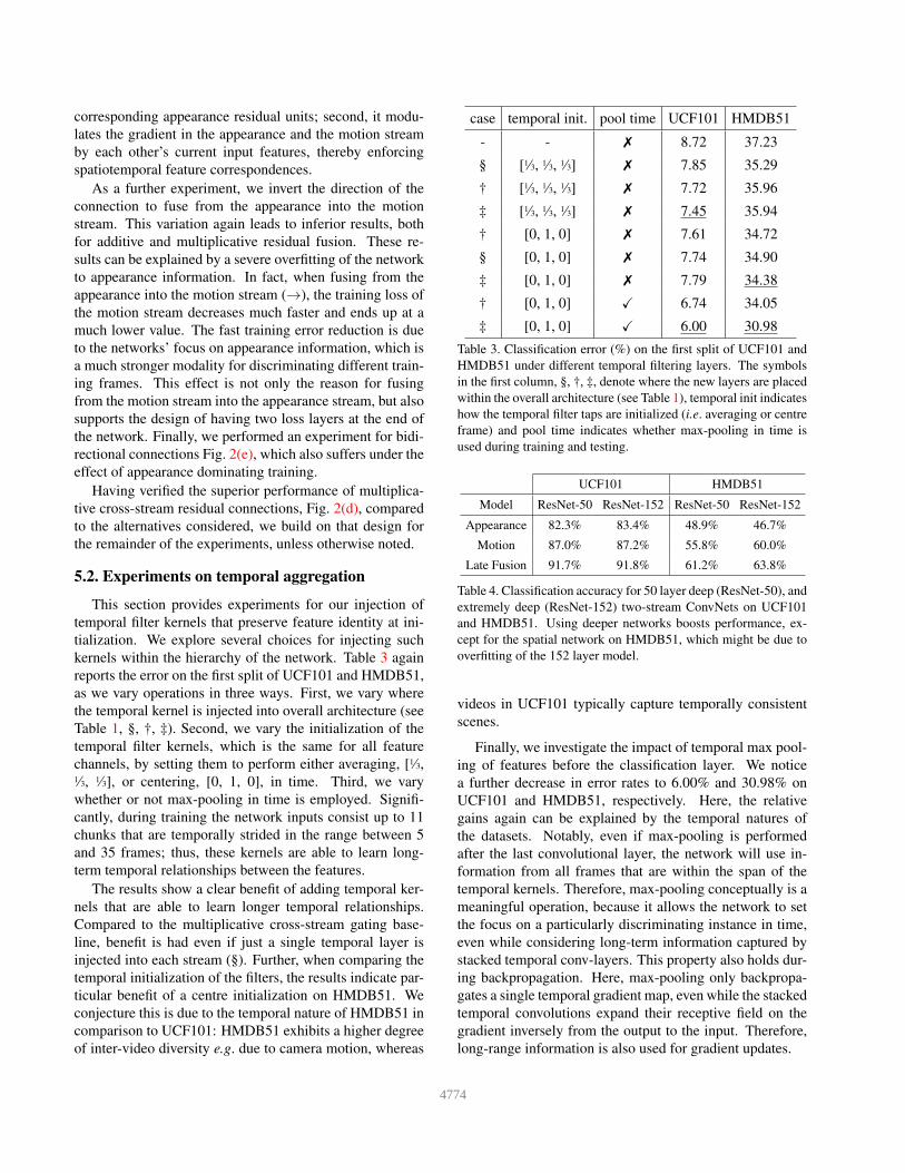
5.2. Experiments on temporal aggregation
This section provides experiments for our injection of
temporal filter kernels that preserve feature identity at ini-
tialization. We explore several choices for injecting such
kernels within the hierarchy of the network. Table 3 again
reports the error on the first split of UCF101 and HMDB51,
as we vary operations in three ways. First, we vary where
the temporal kernel is injected into overall architecture (see
Table 1, §, †, ‡). Second, we vary the initialization of the
temporal filter kernels, which is the same for all feature
channels, by setting them to perform either averaging, [1⁄3,1⁄3, 1⁄3], or centering, [0, 1, 0], in time. Third, we vary
whether or not max-pooling in time is employed. Signifi-
cantly, during training the network inputs consist up to 11
chunks that are temporally strided in the range between 5
and 35 frames; thus, these kernels are able to learn long-
term temporal relationships between the features.
The results show a clear benefit of adding temporal ker-
nels that are able to learn longer temporal relationships.
Compared to the multiplicative cross-stream gating base-
line, benefit is had even if just a single temporal layer is
injected into each stream (§). Further, when comparing the
temporal initialization of the filters, the results indicate par-
ticular benefit of a centre initialization on HMDB51. We
conjecture this is due to the temporal nature of HMDB51 in
comparison to UCF101: HMDB51 exhibits a higher degree
of inter-video diversity e.g. due to camera motion, whereas
case temporal init. pool time UCF101 HMDB51
- - ✗ 8.72 37.23
§ [1⁄3, 1⁄3, 1⁄3] ✗ 7.85 35.29
† [1⁄3, 1⁄3, 1⁄3] ✗ 7.72 35.96
‡ [1⁄3, 1⁄3, 1⁄3] ✗ 7.45 35.94
† [0, 1, 0] ✗ 7.61 34.72
§ [0, 1, 0] ✗ 7.74 34.90
‡ [0, 1, 0] ✗ 7.79 34.38
† [0, 1, 0] X 6.74 34.05
‡ [0, 1, 0] X 6.00 30.98
Table 3. Classification error (%) on the first split of UCF101 and
HMDB51 under different temporal filtering layers. The symbols
in the first column, §, †, ‡, denote where the new layers are placed
within the overall architecture (see Table 1), temporal init indicates
how the temporal filter taps are initialized (i.e. averaging or centre
frame) and pool time indicates whether max-pooling in time is
used during training and testing.
UCF101 HMDB51
Model ResNet-50 ResNet-152 ResNet-50 ResNet-152
Appearance 82.3% 83.4% 48.9% 46.7%
Motion 87.0% 87.2% 55.8% 60.0%
Late Fusion 91.7% 91.8% 61.2% 63.8%
Table 4. Classification accuracy for 50 layer deep (ResNet-50), and
extremely deep (ResNet-152) two-stream ConvNets on UCF101
and HMDB51. Using deeper networks boosts performance, ex-
cept for the spatial network on HMDB51, which might be due to
overfitting of the 152 layer model.
videos in UCF101 typically capture temporally consistent
scenes.
Finally, we investigate the impact of temporal max pool-
ing of features before the classification layer. We notice
a further decrease in error rates to 6.00% and 30.98% on
UCF101 and HMDB51, respectively. Here, the relative
gains again can be explained by the temporal natures of
the datasets. Notably, even if max-pooling is performed
after the last convolutional layer, the network will use in-
formation from all frames that are within the span of the
temporal kernels. Therefore, max-pooling conceptually is a
meaningful operation, because it allows the network to set
the focus on a particularly discriminating instance in time,
even while considering long-term information captured by
stacked temporal conv-layers. This property also holds dur-
ing backpropagation. Here, max-pooling only backpropa-
gates a single temporal gradient map, even while the stacked
temporal convolutions expand their receptive field on the
gradient inversely from the output to the input. Therefore,
long-range information is also used for gradient updates.
4774
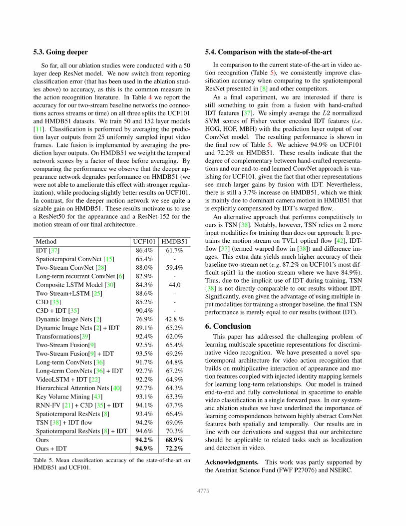
5.3. Going deeper
So far, all our ablation studies were conducted with a 50
layer deep ResNet model. We now switch from reporting
classification error (that has been used in the ablation stud-
ies above) to accuracy, as this is the common measure in
the action recognition literature. In Table 4 we report the
accuracy for our two-stream baseline networks (no connec-
tions across streams or time) on all three splits the UCF101
and HMDB51 datasets. We train 50 and 152 layer models
[11]. Classification is performed by averaging the predic-
tion layer outputs from 25 uniformly sampled input video
frames. Late fusion is implemented by averaging the pre-
diction layer outputs. On HMDB51 we weight the temporal
network scores by a factor of three before averaging. By
comparing the performance we observe that the deeper ap-
pearance network degrades performance on HMDB51 (we
were not able to ameliorate this effect with stronger regular-
ization), while producing slightly better results on UCF101.
In contrast, for the deeper motion network we see quite a
sizable gain on HMDB51. These results motivate us to use
a ResNet50 for the appearance and a ResNet-152 for the
motion stream of our final architecture.
Method UCF101 HMDB51
IDT [37] 86.4% 61.7%
Spatiotemporal ConvNet [15] 65.4% -
Two-Stream ConvNet [28] 88.0% 59.4%
Long-term recurrent ConvNet [6] 82.9% -
Composite LSTM Model [30] 84.3% 44.0
Two-Stream+LSTM [25] 88.6% -
C3D [35] 85.2% -
C3D + IDT [35] 90.4% -
Dynamic Image Nets [2] 76.9% 42.8 %
Dynamic Image Nets [2] + IDT 89.1% 65.2%
Transformations[39] 92.4% 62.0%
Two-Stream Fusion[9] 92.5% 65.4%
Two-Stream Fusion[9] + IDT 93.5% 69.2%
Long-term ConvNets [36] 91.7% 64.8%
Long-term ConvNets [36] + IDT 92.7% 67.2%
VideoLSTM + IDT [22] 92.2% 64.9%
Hierarchical Attention Nets [40] 92.7% 64.3%
Key Volume Mining [43] 93.1% 63.3%
RNN-FV [21] + C3D [35] + IDT 94.1% 67.7%
Spatiotemporal ResNets [8] 93.4% 66.4%
TSN [38] + IDT flow 94.2% 69.0%
Spatiotemporal ResNets [8] + IDT 94.6% 70.3%
Ours 94.2% 68.9%
Ours + IDT 94.9% 72.2%
Table 5. Mean classification accuracy of the state-of-the-art on
HMDB51 and UCF101.
5.4. Comparison with the stateoftheart
In comparison to the current state-of-the-art in video ac-
tion recognition (Table 5), we consistently improve clas-
sification accuracy when comparing to the spatiotemporal
ResNet presented in [8] and other competitors.
As a final experiment, we are interested if there is
still something to gain from a fusion with hand-crafted
IDT features [37]. We simply average the L2 normalized
SVM scores of Fisher vector encoded IDT features (i.e.
HOG, HOF, MBH) with the prediction layer output of our
ConvNet model. The resulting performance is shown in
the final row of Table 5. We achieve 94.9% on UCF101
and 72.2% on HMDB51. These results indicate that the
degree of complementary between hand-crafted representa-
tions and our end-to-end learned ConvNet approach is van-
ishing for UCF101, given the fact that other representations
see much larger gains by fusion with IDT. Nevertheless,
there is still a 3.7% increase on HMDB51, which we think
is mainly due to dominant camera motion in HMDB51 that
is explicitly compensated by IDT’s warped flow.
An alternative approach that performs competitively to
ours is TSN [38]. Notably, however, TSN relies on 2 more
input modalities for training than does our approach: It pre-
trains the motion stream on TVL1 optical flow [42], IDT-
flow [37] (termed warped flow in [38]) and difference im-
ages. This extra data yields much higher accuracy of their
baseline two-stream net (e.g. 87.2% on UCF101’s most dif-
ficult split1 in the motion stream where we have 84.9%).
Thus, due to the implicit use of IDT during training, TSN
[38] is not directly comparable to our results without IDT.
Significantly, even given the advantage of using multiple in-
put modalities for training a stronger baseline, the final TSN
performance is merely equal to our results (without IDT).
6. Conclusion
This paper has addressed the challenging problem of
learning multiscale spacetime representations for discrimi-
native video recognition. We have presented a novel spa-
tiotemporal architecture for video action recognition that
builds on multiplicative interaction of appearance and mo-
tion features coupled with injected identity mapping kernels
for learning long-term relationships. Our model is trained
end-to-end and fully convolutional in spacetime to enable
video classification in a single forward pass. In our system-
atic ablation studies we have underlined the importance of
learning correspondences between highly abstract ConvNet
features both spatially and temporally. Our results are in
line with our derivations and suggest that our architecture
should be applicable to related tasks such as localization
and detection in video.
Acknowledgments. This work was partly supported by
the Austrian Science Fund (FWF P27076) and NSERC.
4775
References
[1] N. Ballas, L. Yao, C. Pal, and A. Courville. Delving deeper
into convolutional networks for learning video representa-
tions. In Proc. ICLR, 2016. 2, 5[2] H. Bilen, B. Fernando, E. Gavves, A. Vedaldi, and S. Gould.
Dynamic image networks for action recognition. In Proc.
CVPR, 2016. 2, 8[3] N. Dalal, B. Triggs, and C. Schmid. Human detection using
oriented histograms of flow and appearance. In Proc. ECCV,
2006. 2[4] K. G. Derpanis, M. Sizintsev, K. Cannons, and R. P. Wildes.
Action spotting and recognition based on a spatiotemporal
orientation analysis. IEEE PAMI, 35(3):527–540, 2013. 2[5] P. Dollar, V. Rabaud, G. Cottrell, and S. Belongie. Behav-
ior recognition via sparse spatio-temporal features. In Work-
shop on Visual Surveillance and Performance Evaluation of
Tracking and Surveillance, in conjunction with the ICCV,
2005. 2[6] J. Donahue, L. A. Hendricks, S. Guadarrama, M. Rohrbach,
S. Venugopalan, K. Saenko, and T. Darrell. Long-term recur-
rent convolutional networks for visual recognition and de-
scription. In Proc. CVPR, 2015. 8[7] C. Feichtenhofer, A. Pinz, and R. Wildes. Dynamically en-
coded actions based on spacetime saliency. In Proc. CVPR,
2015. 2[8] C. Feichtenhofer, A. Pinz, and R. Wildes. Spatiotemporal
residual networks for video action recognition. In NIPS,
2016. 1, 2, 3, 4, 6, 8[9] C. Feichtenhofer, A. Pinz, and A. Zisserman. Convolutional
two-stream network fusion for video action recognition. In
Proc. CVPR, 2016. 2, 4, 5, 6, 8[10] M. Goudreau, C. Giles, S. Chakradhar, and D. Chen. First-
order versus second-order single-layer recurrent neural net-
works. IEEE Transactions on Neural Networks, 5:511–513,
1994. 3[11] K. He, X. Zhang, S. Ren, and J. Sun. Deep residual learning
for image recognition. In Proc. CVPR, 2016. 1, 2, 4, 5, 8[12] K. He, X. Zhang, S. Ren, and J. Sun. Identity mappings in
deep residual networks. In Proc. ECCV, 2016. 2, 6[13] S. Ioffe and C. Szegedy. Batch normalization: Accelerating
deep network training by reducing internal covariate shift. In
Proc. ICML, 2015. 2, 5[14] S. Ji, W. Xu, M. Yang, and K. Yu. 3D convolutional neu-
ral networks for human action recognition. IEEE PAMI,
35(1):221–231, 2013. 2[15] A. Karpathy, G. Toderici, S. Shetty, T. Leung, R. Sukthankar,
and L. Fei-Fei. Large-scale video classification with convo-
lutional neural networks. In Proc. CVPR, 2014. 2, 8[16] A. Klaser, M. Marszałek, and C. Schmid. A spatio-temporal
descriptor based on 3d-gradients. In Proc. BMVC., 2008. 2[17] A. Krizhevsky, I. Sutskever, and G. E. Hinton. ImageNet
classification with deep convolutional neural networks. In
NIPS, 2012. 2[18] H. Kuehne, H. Jhuang, E. Garrote, T. Poggio, and T. Serre.
HMDB: a large video database for human motion recogni-
tion. In Proc. ICCV, 2011. 6[19] I. Laptev, M. Marszalek, C. Schmid, and B. Rozenfeld.
Learning realistic human actions from movies. In Proc.
CVPR, 2008. 2
[20] Q. V. Le, W. Y. Zou, S. Y. Yeung, and A. Y. Ng. Learn-
ing hierarchical invariant spatio-temporal features for action
recognition with independent subspace analysis. In Proc.
CVPR, 2011. 2[21] G. Lev, G. Sadeh, B. Klein, and L. Wolf. RNN Fisher vectors
for action recognition and image annotation. In Proc. ECCV,
2016. 8[22] Z. Li, E. Gavves, M. Jain, and C. G. Snoek. VideoLSTM
convolves, attends and flows for action recognition. arXiv
preprint arXiv:1607.01794, 2016. 2, 8[23] B. Mahasseni and S. Todorovic. Regularizing long short
term memory with 3D human-skeleton sequences for action
recognition. In Proc. CVPR, 2016. 2[24] R. Memisevic and G. E. Hinton. Learning to represent spatial
transformations with factored higher-order boltzmann ma-
chines. Neural Computation, 22(6):1473–1492, 2010. 3[25] J. Y.-H. Ng, M. Hausknecht, S. Vijayanarasimhan,
O. Vinyals, R. Monga, and G. Toderici. Beyond short snip-
pets: Deep networks for video classification. In Proc. CVPR,
2015. 2, 8[26] J. Oh, X. Guo, H. Lee, R. L. Lewis, and S. Singh. Action-
conditional video prediction using deep networks in atari
games. In NIPS, 2015. 3[27] S. Sharma, R. Kiros, and R. Salakhutdinov. Action recogni-
tion using visual attention. In NIPS workshop on Time Series.
2015. 2[28] K. Simonyan and A. Zisserman. Two-stream convolutional
networks for action recognition in videos. In NIPS, 2014. 1,
2, 4, 5, 6, 8[29] K. Soomro, A. R. Zamir, and M. Shah. UCF101: A dataset of
101 human actions calsses from videos in the wild. Technical
Report CRCV-TR-12-01, 2012. 6[30] N. Srivastava, E. Mansimov, and R. Salakhutdinov. Unsu-
pervised learning of video representations using LSTMs. In
Proc. ICML, 2015. 8[31] C. Szegedy, W. Liu, Y. Jia, P. Sermanet, S. Reed,
D. Anguelov, D. Erhan, V. Vanhoucke, and A. Rabinovich.
Going deeper with convolutions. In Proc. CVPR, 2015. 4[32] C. Szegedy, V. Vanhoucke, S. Ioffe, J. Shlens, and Z. Wojna.
Rethinking the inception architecture for computer vision.
arXiv preprint arXiv:1512.00567, 2015. 2[33] G. W. Taylor, R. Fergus, Y. LeCun, and C. Bregler. Convolu-
tional learning of spatio-temporal features. In Proc. ECCV,
2010. 2[34] G. W. Taylor and G. E. Hinton. Factored conditional re-
stricted boltzmann machines for modeling motion style. In
Proc. ICML, 2009. 3[35] D. Tran, L. Bourdev, R. Fergus, L. Torresani, and M. Paluri.
Learning spatiotemporal features with 3D convolutional net-
works. In Proc. ICCV, 2015. 2, 8[36] G. Varol, I. Laptev, and C. Schmid. Long-term temporal con-
volutions for action recognition. arXiv:1604.04494, 2016. 2,
4, 8[37] H. Wang and C. Schmid. Action recognition with improved
trajectories. In Proc. ICCV, 2013. 2, 8[38] L. Wang, Y. Xiong, Z. Wang, Y. Qiao, D. Lin, X. Tang, and
L. Val Gool. Temporal segment networks: Towards good
practices for deep action recognition. In ECCV, 2016. 8[39] X. Wang, A. Farhadi, and A. Gupta. Actions ˜ transforma-
tions. In Proc. CVPR, 2016. 2, 5, 8
4776
[40] Y. Wang, S. Wang, J. Tang, N. O’Hare, Y. Chang, and
B. Li. Hierarchical attention network for action recognition
in videos. arXiv preprint arXiv:1607.06416, 2016. 2, 8[41] Y. Wu, S. Zhang, Y. Zhang, Y. Bengio, and R. Salakhutdinov.
On multiplicative integration with recurrent neural networks.
In NIPS, 2016. 4[42] C. Zach, T. Pock, and H. Bischof. A duality based approach
for realtime TV-L1 optical flow. In Proc. DAGM, pages 214–
223, 2007. 5, 8[43] W. Zhu, J. Hu, G. Sun, X. Cao, and Y. Qiao. A key vol-
ume mining deep framework for action recognition. In Proc.
CVPR, 2016. 2, 8
4777