Special Relativity and Maxwell Equations

by

Bernd A. Berg

Department of Physics

Florida State University

Tallahassee, FL 32306, USA.

Copyright c© by the author.

Chapter 1

A self-contained summary of the theory of special relativity is given, which provides the

space-time frame for classical electrodynamics. Historically [2] special relativity emerged

out of electromagnetism. Nowadays, is deserves to be emphasized that special relativity

restricts severely the possibilities for electromagnetic equations.

1.1 Special Relativity

Let us deal with space and time in vacuum. The conventional time unit is one

second [s]. (1.1)

Here, and in the following abbreviations for units are placed in brackets [ ]. For a long time

period the second was defined in terms of the rotation of the earth as 160× 1

60× 1

24of the mean

solar day. Nowadays most accurate time measurements rely on atomic clocks. They work

by tuning a electric frequency into resonance with some atomic transition. Consequently,

the second has been re–defined, so that the frequency of the light between the two hyperfine

levels of the ground state of the cesium 132Cs atom is now exactly 9,192,631,770 cycles per

second.

Special relativity is founded on two basic postulates:

1. Galilee invariance: The laws of nature are independent of any uniform, translational

motion of the reference frame.

This postulate gives rise to a triple infinite set of reference frames moving with constant

velocities relative to one another. They are called inertial frames. For a freely moving

body, i.e. a body which is not acted upon by an external force, inertial systems exist. The

differential equations which describe physical laws take the same form in all inertial frames.

Galilee invariance was known long before Einstein.

2. The speed c of light in empty space is independent of the motion of its source.

CHAPTER 1. 2

The second Postulate was introduced by Einstein 1905 [2]. It implies that c takes the

same constant value in all inertial frames. Transformations between inertial frames follow,

which have far reaching physical consequences.

The distance unit

1 meter [m] = 100 centimeters [cm] (1.2)

was originally defined by two scratches on a bar made of platinum–iridium alloy kept at the

International Bureau of Weights and Measures in Sevres, France. As measurements of the

speed of light have become increasingly accurate, it has become most appropriate to exploit

Postulate 2 to define the distance unit. The standard meter is now defined [6] as the distance

traveled by light in empty space during the time of 1/299,792,458 [s]. This makes the speed

of light exactly

c = 299, 792, 458 [m/s]. (1.3)

1.1.1 Natural Units

The units for second (1.1 and meter (1.2) are not independent, as the speed of light is an

universal constant. This allows to define natural units, which are frequently used in nuclear,

particle and astro physics. They define

c = 1 (1.4)

as a dimensionless constant, and

1 [s] = 299, 792, 458 [m]

holds. The advantage of natural units is that factors of c disappear in calculations. The

disadvantage is that, for converting back to conventional units, the appropriate factors have

to be recovered by dimensional analysis. For instance, if time is given in seconds x = t in

natural units converts to x = ct with x in meters and c given by (1.3).

1.1.2 Definition of distances and synchronization of clocks

Let us relate the introduced concepts of Galilee invariance and of a constant speed of light to

physical measurements and reduce measurements of spatial distances to time measurements.

Let us consider an inertial frame K with coordinates (t, ~x). We like to place observers at rest

at different places ~x in K. The observers are equipped with clocks of identical making, to

define the time t at ~x. The origin ~x = 0, in other notation (t,~0), of K is defined by placing

observer O0 and his clock there. We like to place another observer O1 at ~x1 to define (t, ~x1).

How can O1 know to be at ~x1? By using a mirror he can reflect light flashed by observer O0

at him. Observer O0 may measure the polar and azimuthal angles (θ, φ) at which he emits

the light and

|~x1| = c△t/2 ,

CHAPTER 1. 3

where △t is the time light needs to travel to O1 and back. This determines ~x1 and he can

signal this information to O1. By repeating the measurement, he can make sure that O1 is

not moving with respect to K. For an idealized, force free environment the observers will

then never start moving with respect to one another. O1 synchronizes his clock by setting it

to

t1 = t0 + |~x1|/c

at the instant receiving the signal. If O0 flashes again his instant time t01 over to O1, the

clock of O1 will show time t11 = t01 + |~x1|/c at the instant of receiving the signal. In the

same way the time t can be defined at any desired point ~x in K.

Now we consider an inertial frame K ′ with coordinates (t′, ~x′), moving with constant

velocity ~v with respect to K. The origin of K ′ is defined through a third observer O′0. What

does it mean that O′0 moves with constant velocity ~v with respect to O0? At times te01 and

te02 observer O0 may flash light signals (the superscript e stands for “emit”) at O′0, which are

reflected and arrive back after time intervals △t01 and △t02. From principle 2 it follows that

the reflected light needs the same time (measured by O0 in K) to travel from O′0 to O0, as

it needed to travel from O0 to O′0. Hence, O0 concludes that O′

0 received the signal at

t0i = te0i + △t0i/2, (i = 1, 2) (1.5)

in the O0 time. This simple equation becomes quite complicated for non-relativistic physics,

because the speed on the return path would then be distinct from that on the arrival path

(consider for instance elastic scattering of a very light particle on a heavy surface). The

constant velocity of light implies that relativistic distance measurements are simpler than

such non-relativistic measurements. For observer O0 the positions ~x01 and ~x02 are now

defined through the angles (θ0i, φ0i) and

|~x0i| = △t0i c/2, (i = 1, 2) . (1.6)

For the assumed force free environment observer O0 can conclude that O′0 moves with respect

to him with uniform velocity

~v = (~x02 − ~x01)/(t02 − t01) . (1.7)

Actually, one measurement is sufficient to obtain the velocity when one employs the

relativistic Doppler effect as discussed later in section 1.1.8. O0 may repeat the procedure

at later times to check that O′o moves indeed with uniform velocity.

Similarly, observer O′0 finds out that O0 moves with velocity ~v ′ = −~v. According to

principle 1, observers in K ′ can now go ahead to define t′ for any point ~x ′ in K ′. The

equation of motion for the origin of K ′ is as observed by O0 is

~x (~x′

= 0) = ~x0 + ~v t, (1.8)

CHAPTER 1. 4

with ~x0 = ~x01 − ~v t01, expressesing the fact that for t = t01 observer O′0 is at ~x01. Shifting

his space convention by a constant vector, observer O0 can achieve ~x0 = 0, so that equation

(1.8) becomes

~x (~x′

= 0) = ~v t.

Similarly, observer O′0 may choose his space convention so that

~x′

(~x = 0) = −~v t′

holds.

1.1.3 Lorentz invariance and Minkowski space

Having defined time and space operationally, let us focus on a more abstract discussion. We

consider the two inertial frames with uniform relative motion ~v: K with coordinates (t, ~x) and

K ′ with coordinates (t′, ~x ′). We demand that at time t = t′ = 0 their two origins coincide.

Now, imagine a spherical shell of radiation originating at time t = 0 from ~x = ~x ′ = 0. The

propagation of the wavefront is described by

c2t2 − x2 − y2 − z2 = 0 in K, (1.9)

and by

c2t′ 2 − x′ 2 − y′ 2 − z′ 2 = 0 in K ′. (1.10)

We define 4-vectors (α = 0, 1, 2, 3) by

(xα) =(ct~x

)and (xα) = (ct, −~x) . (1.11)

Due to a more general notation, which is explained in section 1.1.5, the components xα are

called contravariant and the components xα covariant. In matrix notation the contravariant

4-vector (xα) is represented by a column and the covariant 4-vector (xα) as a row.

The Einstein summation convention is defined by

xαxα =

3∑

α=0

xαxα, (1.12)

and will be employed from here on. Equations (1.9) and (1.10) read then

xαxα = x′αx

′α = 0 . (1.13)

(Homogeneous) Lorentz transformations are defined as the group of transformations which

leave the distance s2 = xαxα invariant:

xαxα = x′αx

′α = s2 . (1.14)

CHAPTER 1. 5

x0

x1

Future

Elsewhere Elsewhere

Past

A

B

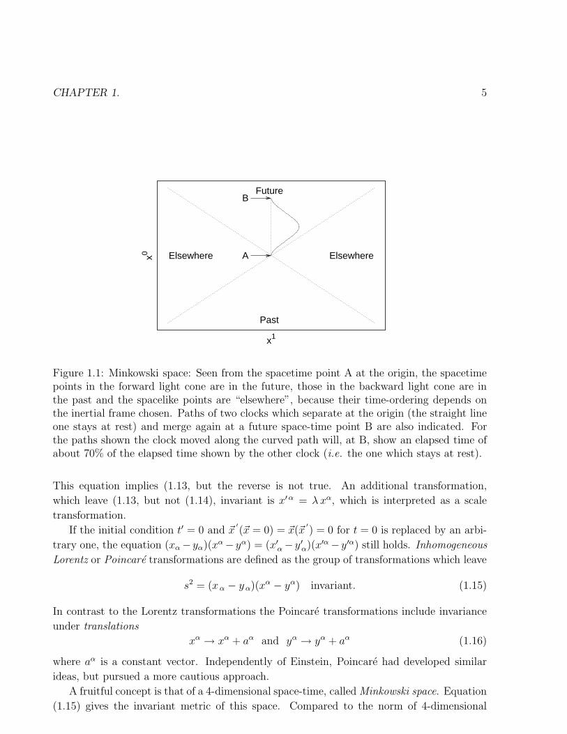
Figure 1.1: Minkowski space: Seen from the spacetime point A at the origin, the spacetimepoints in the forward light cone are in the future, those in the backward light cone are inthe past and the spacelike points are “elsewhere”, because their time-ordering depends onthe inertial frame chosen. Paths of two clocks which separate at the origin (the straight lineone stays at rest) and merge again at a future space-time point B are also indicated. Forthe paths shown the clock moved along the curved path will, at B, show an elapsed time ofabout 70% of the elapsed time shown by the other clock (i.e. the one which stays at rest).

This equation implies (1.13, but the reverse is not true. An additional transformation,

which leave (1.13, but not (1.14), invariant is x′α = λ xα, which is interpreted as a scale

transformation.

If the initial condition t′ = 0 and ~x′(~x = 0) = ~x(~x

′) = 0 for t = 0 is replaced by an arbi-

trary one, the equation (xα − yα)(xα − yα) = (x′α − y′α)(x′α − y′α) still holds. Inhomogeneous

Lorentz or Poincare transformations are defined as the group of transformations which leave

s2 = (xα − yα)(xα − yα) invariant. (1.15)

In contrast to the Lorentz transformations the Poincare transformations include invariance

under translations

xα → xα + aα and yα → yα + aα (1.16)

where aα is a constant vector. Independently of Einstein, Poincare had developed similar

ideas, but pursued a more cautious approach.

A fruitful concept is that of a 4-dimensional space-time, called Minkowski space. Equation

(1.15) gives the invariant metric of this space. Compared to the norm of 4-dimensional

CHAPTER 1. 6

Euclidean space, the crucial difference is the relative minus sign between time and space

components. The light cone of a 4-vector xα0 is defined as the set of vectors xα which satisfy

(x− x0)2 = (xα − x0α) (xα − xα

0 ) = 0.

The light cone separates events which are timelike and spacelike with respect to xα0 , namely

(x− x0)2 > 0 for timelike

and

(x− x0)2 < 0 for spacelike.

We shall see soon, compare equation (1.22), that the time ordering of spacelike points is

distinct in different inertial frames, whereas it is the same for timelike points. For the choice

xα0 = 0 this Minkowski space situation is depicted in figure 1.1. On the abscissa we have the

projection of the three dimensional Euclidean space on r = |~x|. The regions future and past

of this figure are the timelike points of x0 = 0, whereas elsewhere are the spacelike points.

To understand special relativity in some depth, we have to explore Lorentz and Poincare

transformations in some details. Before we come to this, we consider the two-dimensional

case and introduce some relevant calculus in the next two sections.

1.1.4 Two-Dimensional Relativistic Kinematics

We chose now ~v in x-direction and restrict the discussion of to the x-axis:

c2t2 − (x1)2 = c2t′2 − (x′ 1)2 (1.17)

It is customary to define x0 = ct, x′ 0 = ct′ and β = v/c. We are looking for a linear

transformation (x

′ 0

x′ 1

)=(a bd e

)(x0

x1

)(1.18)

which fulfills (1.17) for all x0, x1. Choosing(x0

x1

)=(

10

)gives

a2 − d2 = 1 ⇒ a = cosh(ζ), d = ± sinh(ζ) (1.19)

and choosing(x0

x1

)=(

01

)gives

b2 − e2 = −1 ⇒ e = cosh(η), b = ± sinh(η) . (1.20)

Using now(x0

x1

)=(

11

)yields

[cosh(ζ) + sinh(η)]2 − [sinh(ζ) + cosh(η)]2 = 0 ⇒ ζ = η.

CHAPTER 1. 7

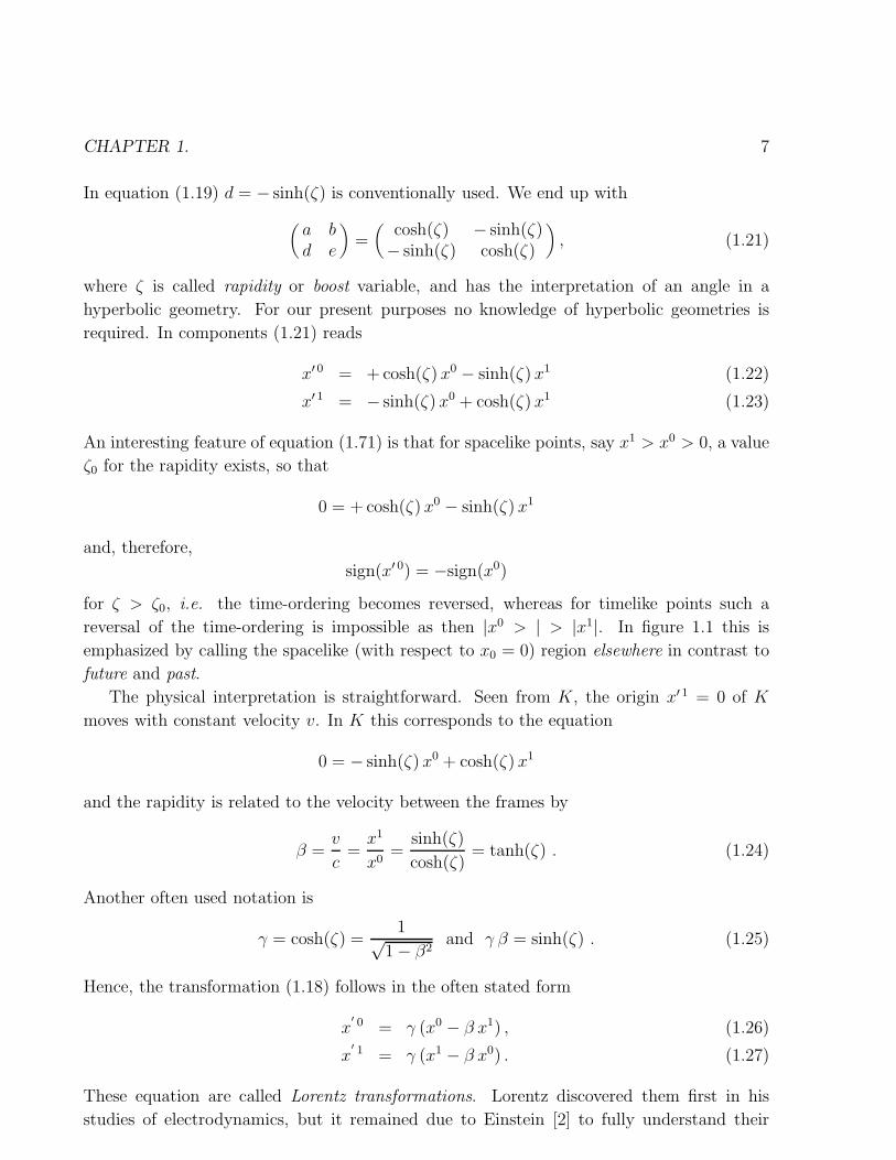
In equation (1.19) d = − sinh(ζ) is conventionally used. We end up with

(a bd e

)=(

cosh(ζ) − sinh(ζ)− sinh(ζ) cosh(ζ)

), (1.21)

where ζ is called rapidity or boost variable, and has the interpretation of an angle in a

hyperbolic geometry. For our present purposes no knowledge of hyperbolic geometries is

required. In components (1.21) reads

x′ 0 = + cosh(ζ) x0 − sinh(ζ) x1 (1.22)

x′ 1 = − sinh(ζ) x0 + cosh(ζ) x1 (1.23)

An interesting feature of equation (1.71) is that for spacelike points, say x1 > x0 > 0, a value

ζ0 for the rapidity exists, so that

0 = + cosh(ζ) x0 − sinh(ζ) x1

and, therefore,

sign(x′ 0) = −sign(x0)

for ζ > ζ0, i.e. the time-ordering becomes reversed, whereas for timelike points such a

reversal of the time-ordering is impossible as then |x0 > | > |x1|. In figure 1.1 this is

emphasized by calling the spacelike (with respect to x0 = 0) region elsewhere in contrast to

future and past.

The physical interpretation is straightforward. Seen from K, the origin x′ 1 = 0 of K

moves with constant velocity v. In K this corresponds to the equation

0 = − sinh(ζ) x0 + cosh(ζ) x1

and the rapidity is related to the velocity between the frames by

β =v

c=x1

x0=

sinh(ζ)

cosh(ζ)= tanh(ζ) . (1.24)

Another often used notation is

γ = cosh(ζ) =1√

1 − β2and γ β = sinh(ζ) . (1.25)

Hence, the transformation (1.18) follows in the often stated form

x′ 0 = γ (x0 − β x1) , (1.26)

x′ 1 = γ (x1 − β x0) . (1.27)

These equation are called Lorentz transformations. Lorentz discovered them first in his

studies of electrodynamics, but it remained due to Einstein [2] to fully understand their

CHAPTER 1. 8

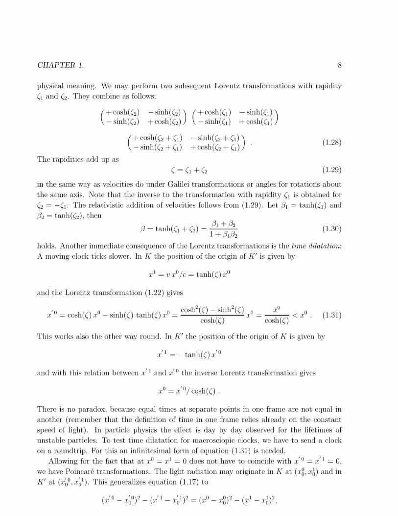
physical meaning. We may perform two subsequent Lorentz transformations with rapidity

ζ1 and ζ2. They combine as follows:

(+ cosh(ζ2) − sinh(ζ2)− sinh(ζ2) + cosh(ζ2)

) (+ cosh(ζ1) − sinh(ζ1)− sinh(ζ1) + cosh(ζ1)

)

(+ cosh(ζ2 + ζ1) − sinh(ζ2 + ζ1)− sinh(ζ2 + ζ1) + cosh(ζ2 + ζ1)

). (1.28)

The rapidities add up as

ζ = ζ1 + ζ2 (1.29)

in the same way as velocities do under Galilei transformations or angles for rotations about

the same axis. Note that the inverse to the transformation with rapidity ζ1 is obtained for

ζ2 = −ζ1. The relativistic addition of velocities follows from (1.29). Let β1 = tanh(ζ1) and

β2 = tanh(ζ2), then

β = tanh(ζ1 + ζ2) =β1 + β2

1 + β1β2(1.30)

holds. Another immediate consequence of the Lorentz transformations is the time dilatation:

A moving clock ticks slower. In K the position of the origin of K ′ is given by

x1 = v x0/c = tanh(ζ) x0

and the Lorentz transformation (1.22) gives

x′ 0 = cosh(ζ) x0 − sinh(ζ) tanh(ζ) x0 =

cosh2(ζ) − sinh2(ζ)

cosh(ζ)x0 =

x0

cosh(ζ)< x0 . (1.31)

This works also the other way round. In K ′ the position of the origin of K is given by

x′ 1 = − tanh(ζ) x

′ 0

and with this relation between x′ 1 and x

′ 0 the inverse Lorentz transformation gives

x0 = x′ 0/ cosh(ζ) .

There is no paradox, because equal times at separate points in one frame are not equal in

another (remember that the definition of time in one frame relies already on the constant

speed of light). In particle physics the effect is day by day observed for the lifetimes of

unstable particles. To test time dilatation for macrosciopic clocks, we have to send a clock

on a roundtrip. For this an infinitesimal form of equation (1.31) is needed.

Allowing for the fact that at x0 = x1 = 0 does not have to coincide with x′ 0 = x

′ 1 = 0,

we have Poincare transformations. The light radiation may originate in K at (x00, x

10) and in

K ′ at (x′ 00 , x

′ 10 ). This generalizes equation (1.17) to

(x′ 0 − x

′ 00 )2 − (x

′ 1 − x′ 10 )2 = (x0 − x0

0)2 − (x1 − x1

0)2,

CHAPTER 1. 9

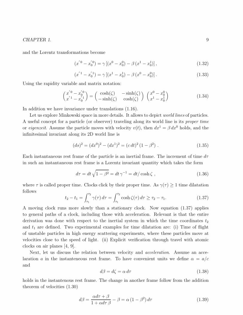
and the Lorentz transformations become

(x′ 0 − x

′ 00 ) = γ [(x0 − x0

0) − β (x1 − x10)] , (1.32)

(x′ 1 − x

′ 10 ) = γ [(x1 − x1

0) − β (x0 − x00)] . (1.33)

Using the rapidity variable and matrix notation:

(x

′ 0 − x′ 00

x′ 1 − x

′ 10

)=(

cosh(ζ) − sinh(ζ)− sinh(ζ) cosh(ζ)

) (x0 − x0

0

x1 − x10

)(1.34)

In addition we have invariance under translations (1.16).

Let us explore Minkowski space in more details. It allows to depict world lines of particles.

A useful concept for a particle (or observer) traveling along its world line is its proper time

or eigenzeit. Assume the particle moves with velocity v(t), then dx1 = β dx0 holds, and the

infinitesimal invariant along its 2D world line is

(ds)2 = (dx0)2 − (dx1)2 = (c dt)2 (1 − β2) . (1.35)

Each instantaneous rest frame of the particle is an inertial frame. The increment of time dτ

in such an instantaneous rest frame is a Lorentz invariant quantity which takes the form

dτ = dt√

1 − β2 = dt γ−1 = dt/ cosh ζ , (1.36)

where τ is called proper time. Clocks click by their proper time. As γ(τ) ≥ 1 time dilatation

follows

t2 − t1 =∫ τ2

τ1γ(τ) dτ =

∫ τ2

τ1cosh ζ(τ) dτ ≥ τ2 − τ1. (1.37)

A moving clock runs more slowly than a stationary clock. Now equation (1.37) applies

to general paths of a clock, including those with acceleration. Relevant is that the entire

derivation was done with respect to the inertial system in which the time coordinates t2and t1 are defined. Two experimental examples for time dilatation are: (i) Time of flight

of unstable particles in high energy scattering experiments, where these particles move at

velocities close to the speed of light. (ii) Explicit verification through travel with atomic

clocks on air planes [4, 9].

Next, let us discuss the relation between velocity and acceleration. Assume an acce-

laration a in the instanteneous rest frame. To have convenient units we define α = a/c

and

dβ = dζ = α dτ (1.38)

holds in the instantenous rest frame. The change in another frame follow from the addition

theorem of velocities (1.30)

dβ =αdτ + β

1 + αdτ β− β = α (1 − β2) dτ (1.39)

CHAPTER 1. 10

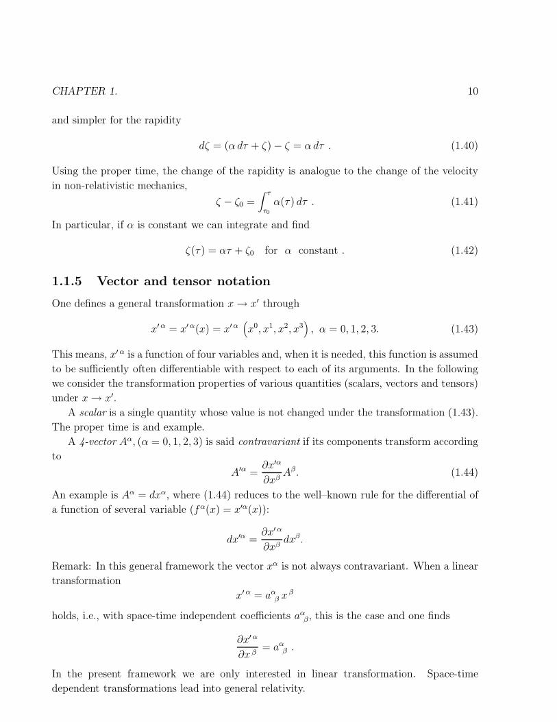
and simpler for the rapidity

dζ = (α dτ + ζ) − ζ = α dτ . (1.40)

Using the proper time, the change of the rapidity is analogue to the change of the velocity

in non-relativistic mechanics,

ζ − ζ0 =∫ τ

τ0α(τ) dτ . (1.41)

In particular, if α is constant we can integrate and find

ζ(τ) = ατ + ζ0 for α constant . (1.42)

1.1.5 Vector and tensor notation

One defines a general transformation x→ x′ through

x′α = x′α(x) = x′α(x0, x1, x2, x3

), α = 0, 1, 2, 3. (1.43)

This means, x′α is a function of four variables and, when it is needed, this function is assumed

to be sufficiently often differentiable with respect to each of its arguments. In the following

we consider the transformation properties of various quantities (scalars, vectors and tensors)

under x→ x′.

A scalar is a single quantity whose value is not changed under the transformation (1.43).

The proper time is and example.

A 4-vector Aα, (α = 0, 1, 2, 3) is said contravariant if its components transform according

to

A′α =∂x′α

∂xβAβ. (1.44)

An example is Aα = dxα, where (1.44) reduces to the well–known rule for the differential of

a function of several variable (fα(x) = x′α(x)):

dx′α =∂x′α

∂xβdxβ.

Remark: In this general framework the vector xα is not always contravariant. When a linear

transformation

x′α = aαβ x

β

holds, i.e., with space-time independent coefficients aαβ, this is the case and one finds

∂x′α

∂xβ= aα

β .

In the present framework we are only interested in linear transformation. Space-time

dependent transformations lead into general relativity.

CHAPTER 1. 11

A 4-vector is said covariant when it transforms like

B′α =

∂xβ

∂x′αBβ . (1.45)

An example is

Bα = ∂α =∂

∂xα, (1.46)

because of∂

∂x′α=∂xβ

∂x′α∂

∂xβ.

The inner or scalar product of two vectors is defined as the product of the components of a

covariant and a contravariant vector:

B · A = BαAα. (1.47)

It follows from (1.44) and (1.45) that the scalar product is an invariant under the transfor-

mation (1.43):

B′ · A′ =∂xβ

∂x′α∂x′α

∂xγBβA

γ =∂xβ

∂xγBβA

γ = δβγBβA

γ = B · A.

Here the Kronecker delta is defined by:

δαβ = δ β

α ={

1 for α = β,0 for α 6= β.

(1.48)

Vectors are rank one tensors. Tensors of general rank k are quantities with k indices, like

for instance

T α1α2......αi...αk

.

The convention is that the upper indices transform contravariant and the lower transform

covariant. For instance, a contravariant tensor of rank two F αβ consists of 16 quantities that

transform according to

F ′αβ =∂x′α

∂xγ

∂x′β

∂xδF γδ.

A covariant tensor of rank two Gαβ transforms as

G′αβ =

∂xγ

∂x′α∂xδ

∂x′βGγδ.

The inner product or contraction with respect to a pair of indices, either on the same tensor or

between different tensors, is defined in analogy with (1.47). One index has to be contravariant

and the other covariant.

A tensor S ...α...β... is said to be symmetric in α and β when

S ...α...β... = S ...β...α....

CHAPTER 1. 12

A tensor A...α...β... is said to be antisymmetric in α and β when

A...α...β... = −A...β...α....

Let S ...α...β be a symmetric and A...α...β be an antisymmetric tensor. It holds

S ...α...β...A...α...β... = 0. (1.49)

Proof:

S ...α...β...A...α...β... = −S ...β...α...A...β...α... = −S ...α...β...A...α...β...,

and consequently zero. The first step exploits symmetry and antisymmetry, and the second

step renames the summation indices. Every tensor can be written as a sum of its symmetric

and antisymmetric parts in two if its indices

T ...α...β... = T ...α...β...S + T ...α...β...

A (1.50)

by simply defining

T ...α...β...S =

1

2

(T ...α...β... + T ...β...α...

)and T ...α...β...

A =1

2

(T ...α...β... − T ...β...α...

). (1.51)

So far the results and definitions are general. We now specialize to Poincare transforma-

tions. The specific geometry of the space–time of special relativity is defined by the invariant

distance s2, see equation (1.15). In differential form, the infinitesimal interval ds defines the

proper time c dτ = ds,

(ds)2 = (dx0)2 − (dx1)2 − (dx2)2 − (dx3)2. (1.52)

Here we have used superscripts on the coordinates in accordance to our insight that dxα is

a contravariant vector. Introducing a metric tensor gαβ we re–write equation (1.52) as

(ds)2 = gαβ dxαdxβ. (1.53)

Comparing (1.52) and (1.53) we see that for special relativity gαβ is diagonal:

g00 = 1, g11 = g22 = g33 = −1 and gαβ = 0 for α 6= β. (1.54)

Comparing (1.53) with the invariant scalar product (1.47), we conclude that

xα = gαβ xβ.

The covariant metric tensor lowers the indices, i.e. transforms a contravariant into a covariant

vector. Correspondingly the contravariant metric tensor gαβ is defined to raise indices:

xα = gαβ xβ.

CHAPTER 1. 13

The last two equations and the symmetry of gαβ imply

gαγ gγβ = δ β

α

for the contraction of contravariant and covariant metric tensors. This is solved by gαβ being

the normalized co–factor of gαβ . For the diagonal matrix (1.54) the result is simply

gαβ = gαβ. (1.55)

Consequently the equations

Aα =(A0

~A

), Aα = (A0,− ~A)

and, compare (1.46),

(∂α) =

(∂

c∂t,∇), (∂α) =

∂c∂t

−∇

. (1.56)

hold. It follows that the 4-divergence of a 4-vector

∂αAα = ∂αAα =

∂A0

∂x0+ ∇ · ~A

and the d’Alembert (4-dimensional Laplace) operator

= ∂α∂α =

(∂

∂x0

)2

−∇2

are invariants. Sometimes the notation △ = ∇2 is used for the (3-dimensional) Laplace

operator.

1.1.6 Lorentz transformations

Let us now construct the Lorentz group. We seek a group of linear transformations

x′α = aαβ x

β , (⇒ ∂x′α

∂xβ= aα

β) (1.57)

such that the scalar product stays invariant:

x′α x′α = a β

α xβ aαγx

γ = xα xα = δβ

γxβxγ.

As the xβxγ are independent, this yields

a βα aα

γ = δβγ ⇔ aαβ a

αγ = gβγ ⇔ aδ

β gδα aαγ = gβγ .

In matrix notation

AgA = g, (1.58)

CHAPTER 1. 14

where g = (gβα) is given by (1.54),

A = (aβα) =

a00 a0

1 a02 a0

3

a10 a1

1 a12 a1

3

a20 a2

1 a22 a2

3

a30 a3

1 a32 a3

3

, (1.59)

and A = (a αβ ) with a α

β = aαβ is the transpose of the matrix A = (aβ

α), explicitly

A = (a αβ ) =

a 00 a 1

0 a 20 a 3

0

a 01 a 1

1 a 21 a 3

1

a 02 a 1

2 a 22 a 3

2

a 03 a 1

3 a 23 a 3

3

=

a00 a1

0 a20 a3

0

a01 a1

1 a21 a3

1

a02 a1

2 a22 a3

2

a03 a1

3 a23 a3

3

. (1.60)

For this definition of the transpose matrix the row indices are contravariant and the column

indices are covariant, vice verse to the definition (1.11) for vectors and, similarly, ordinary

matrices. Certain properties of the transformation matrix A can be deduced from (1.58).

Taking the determinant of both sides gives us det(AgA) = det(g) det(A)2 = det(g). Since

det(g) = −1, we obtain

det(A) = ±1. (1.61)

One distinguishes two classes of transformations. Proper Lorentz transformations are

continuously connected with the identity transformation A = 1. All other Lorentz

transformations are improper. Proper transformations have necessarily det(A) = 1. For

improper Lorentz transformations it is sufficient, but not necessary, to have det(A) = −1.

For instance A = −1 (space and time inversion) is an improper Lorentz transformation with

det(A) = +1.

Next the number of parameters, needed to specify completely a transformation in the

group, follows from (1.58). Since A and g are 4 × 4 matrices, we have 16 equations for

42 = 16 elements of A. But they are not all independent because of symmetry under

transposition. The off-diagonal equations are identical in pairs. Therefore, we have 4+6 = 10

linearly independent equations for the 16 elements of A. This means that there are six free

parameters. In other words, the Lorentz group is a six–parameter group.

In the 19th century Lie invented the subsequent procedure to handle these parameters.

Let us now consider only proper Lorentz transformations. To construct A explicitly, Lie

makes the ansatz

A = eL =∞∑

n=0

Ln

n!,

where L is a 4 × 4 matrix. The determinant of A is

det(A) = det(eL) = eTr(L). (1.62)

Note that det(A) = +1 implies that L is traceless. Equation (1.58) can be written

gAg = A−1. (1.63)

CHAPTER 1. 15

From the definition of L, L and the fact that g2 = 1 we have (note (gLg)n = gLng and

1 = (∑∞

n=0Ln/n!) (

∑∞n=0(−L)n/n!))

A = eL, gAg = egLg and A−1 = e−L .

Therefore, (1.63) is equivalent to

gLg = −L or ˜(gL) = −gL.

The matrix gL is thus antisymmetric and it is left as an exercise to show that the general

form of L is:

L =

0 l01 l02 l03l01 0 l12 l13l02 −l12 0 l23l03 −l13 −l23 0

. (1.64)

It is customary to expand L in terms of six generators:

L = −3∑

i=1

(ωiSi + ζiKi) and A = e−∑

3

i=1(ωiSi+ζiKi). (1.65)

The matrices are defined by

S1 =

0 0 0 00 0 0 00 0 0 −10 0 1 0

, S2 =

0 0 0 00 0 0 10 0 0 00 −1 0 0

, S3 =

0 0 0 00 0 −1 00 1 0 00 0 0 0

, (1.66)

and

K1 =

0 1 0 01 0 0 00 0 0 00 0 0 0

, K2 =

0 0 1 00 0 0 01 0 0 00 0 0 0

, K3 =

0 0 0 10 0 0 00 0 0 01 0 0 0

, (1.67)

They satisfy the following Lie algebra commutation relations:

[Si, Sj ] =3∑

k=1

ǫijkSk, [Si, Kj ] =3∑

k=1

ǫijkKk, [Ki, Kj ] = −3∑

k=1

ǫijkSk,

where the commutator of two matrices is defined by [A,B] = AB −BA. Further ǫijk is the

completely antisymmetric Levi–Cevita tensor. Its definition in n–dimensions is

ǫi1i2...in =

+1 for (i1, i2, ..., in) being an even permutation of (1, 2, ..., n),−1 for (i1, i2, ..., in) being an odd permutation of (1, 2, ..., n),0 otherwise.

(1.68)

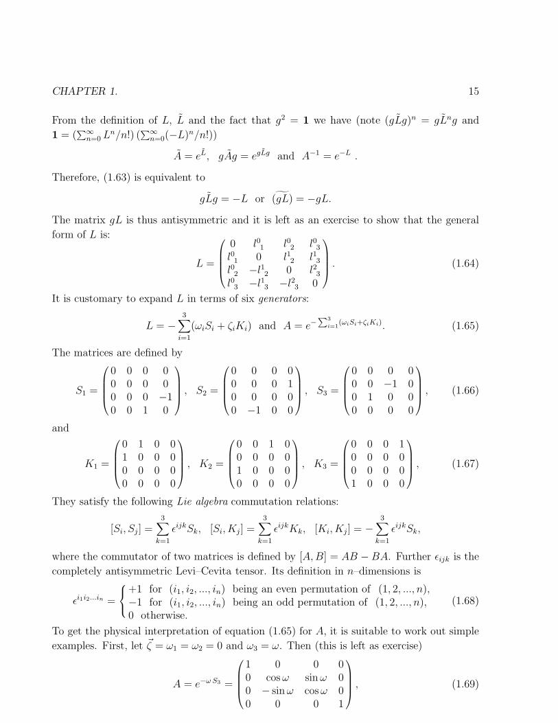
To get the physical interpretation of equation (1.65) for A, it is suitable to work out simple

examples. First, let ~ζ = ω1 = ω2 = 0 and ω3 = ω. Then (this is left as exercise)

A = e−ω S3 =

1 0 0 00 cosω sinω 00 − sinω cosω 00 0 0 1

, (1.69)

CHAPTER 1. 16

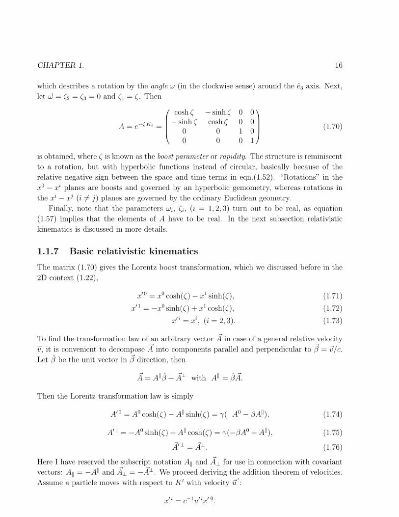
which describes a rotation by the angle ω (in the clockwise sense) around the e3 axis. Next,

let ~ω = ζ2 = ζ3 = 0 and ζ1 = ζ . Then

A = e−ζ K1 =

cosh ζ − sinh ζ 0 0− sinh ζ cosh ζ 0 0

0 0 1 00 0 0 1

(1.70)

is obtained, where ζ is known as the boost parameter or rapidity. The structure is reminiscent

to a rotation, but with hyperbolic functions instead of circular, basically because of the

relative negative sign between the space and time terms in eqn.(1.52). “Rotations” in the

x0 − xi planes are boosts and governed by an hyperbolic gemometry, whereas rotations in

the xi − xj (i 6= j) planes are governed by the ordinary Euclidean geometry.

Finally, note that the parameters ωi, ζi, (i = 1, 2, 3) turn out to be real, as equation

(1.57) implies that the elements of A have to be real. In the next subsection relativistic

kinematics is discussed in more details.

1.1.7 Basic relativistic kinematics

The matrix (1.70) gives the Lorentz boost transformation, which we discussed before in the

2D context (1.22),

x′ 0 = x0 cosh(ζ) − x1 sinh(ζ), (1.71)

x′ 1 = −x0 sinh(ζ) + x1 cosh(ζ), (1.72)

x′ i = xi, (i = 2, 3). (1.73)

To find the transformation law of an arbitrary vector ~A in case of a general relative velocity

~v, it is convenient to decompose ~A into components parallel and perpendicular to ~β = ~v/c.

Let β be the unit vector in ~β direction, then

~A = A‖β + ~A⊥ with A‖ = β ~A.

Then the Lorentz transformation law is simply

A′ 0 = A0 cosh(ζ) − A‖ sinh(ζ) = γ( A0 − βA‖), (1.74)

A′ ‖ = −A0 sinh(ζ) + A‖ cosh(ζ) = γ(−βA0 + A‖), (1.75)

~A′ ⊥ = ~A⊥. (1.76)

Here I have reserved the subscript notation A‖ and ~A⊥ for use in connection with covariant

vectors: A‖ = −A‖ and ~A⊥ = − ~A⊥. We proceed deriving the addition theorem of velocities.

Assume a particle moves with respect to K ′ with velocity ~u′:

x′ i = c−1u′ ix′ 0.

CHAPTER 1. 17

Equations (1.26), (1.27) imply

γ (x1 − βx0) = c−1u′ 1γ (x0 − βx1).

Sorting with respect to x1 and x0 gives

γ

(1 +

u′ 1v

c2

)x1 = c−1γ (u′1 + v) x0 .

Using the definition of the velocity in K, ~x = c−1~u x0, gives

u1 = cx1

x0=

u′1 + v

1 + u′1vc2

. (1.77)

Along similar lines, we obtain for the two other components

ui =u′i

γ(1 + u′1v

c2

) , (i = 2, 3). (1.78)

To derive these equations, ~v was chosen along to the x1-axis. For general ~v one only has to

decompose ~u into its components parallel and perpendicular to the ~v

~u = u‖v + ~u⊥ ,

where v is the unit vector in ~v direction, and obtains

u‖ =u′ ‖ + v

1 + u′ ‖vc2

and ~u⊥ =~u

′ ⊥

γ(1 + u′ ‖v

c2

) . (1.79)

From this addition theorem of velocities it is obvious that the velocity itself is not part of

of a 4-vector. The relativistic generalization is given in subsection (1.1.9). It is left as an

exercise to relate these equations to the addition theorem for the rapidity (1.29.

The concepts of world lines in Minkowski space and proper time (eigenzeit generalized

immediately to 4D. Assume the particle moves with velocity ~v(t), then d~x = ~βdx0 holds,

and the infinitesimal invariant along its world line is

(ds)2 = (dx0)2 − (d~x)2 = (c dt)2 (1 − β2) (1.80)

and the relations (1.36) and (1.37) hold as in 2D.

1.1.8 Plane waves and the relativistic Doppler effect

Let us choose coordinates with respect to an inertial frame K. In complex notation a plane

wave is defined by the equation

W (x) = W (x0, ~x) = W0 exp[ i (k0 x0 − ~k ~x) ] , (1.81)

CHAPTER 1. 18

where W0 = U0 + i V0 is a complex amplitude. The vector ~k is called wave vector. It becomes

a 4-vector (kα) by identifying

k0 = ω/c (1.82)

as its zero-component, where ω is the angular frequency of the wave. Waves of the form

(1.81) may either propagate in a medium (water, air, shock waves, etc.) or in vacuum (light

waves, particle waves in quantum mechanics). We are interested in the latter case, as the

other defines a preferred inertial frame, namely the one where the medium is at rest. The

phase of the wave is defined by

Φ(x) = Φ(x0, ~x) = k0 x0 − ~k ~x = ω t− ~k ~x . (1.83)

When (kα) is a 4-vector, it follows that the phase is a scalar, invariant under Lorentz

transformations

Φ′(x′) = k′α x′α = kα x

α = Φ(x) . (1.84)

That this is correct can be seen as follows: For an observer at a fixed position ~x (note the

term ~k ~x is then constant) the wave performs a periodic motion with period

T =2π

ω=

1

ν, (1.85)

where ν is the frequency. In particular, the phase (and hence the wave) takes identical values

on the two-dimensional hyperplanes perpendicular to ~k. Namely, let k be the unit vector in ~k

direction, by decomposing ~x into components parallel and perpendicular to ~k, ~x = x‖ k+~x⊥,

the phase becomes

Φ = ω t− k x‖ , (1.86)

where k = |~k| is the length of the vector ~k. Phases which differ by multiples of 2π give the

same values for the wave W . For example, when we take V0 = 0, the real part of the wave

becomes

Wx = U0 cos(ω t− k x‖)

and Φ = 0, n 2π, n = ±1,±2, ... describes the wave crests. From (1.86) it follows that the

crests pass by our observer with speed ~u = u k, where

u =ω

kas for Φ = 0 we have x‖ =

ω

kt . (1.87)

Let our observer count the number of wave crests passing by. How has then the wave (1.81)

to be described in another inertial frame K ′? An observer in K ′ who counts the number of

wave crests, passing through the same space-time point at which our first observer already

counts, must get the same number. After all, the coordinates are just labels and the physics

is the same in all systems. When in frame K the wave takes its maximum at the space-

time point (xα) it must also be at its maximum in K ′ at the same space-time point in

appropriately transformed coordinates (x′α). More generally, this is holds for every value of

the phase, because it is a scalar.

CHAPTER 1. 19

As (kα) is a 4-vector the transformation law for angular frequency and wave vector is

just a special case of equations (1.74), (1.75) and (1.76)

k′ 0 = k0 cosh(ζ) − k‖ sinh(ζ) = γ(k0 − βk‖) , (1.88)

k′ ‖ = −k0 sinh(ζ) + k‖ cosh(ζ) = γ(k‖ − βk0) , (1.89)

~k′ ⊥ = ~k⊥ , (1.90)

where the notation k‖ and k⊥ is with respect to the relative velocity of the two frames, ~v.

These transformation equations for the frequency and the wave vector describe the relativistic

Doppler effect. To illustrate their meaning, let us specialize to the case of a light source,

which is emitted in K and the observer K ′ moves in wave vector direction away from the

source, i.e., ~v ‖ ~k. The equation for the wave speed (1.87) implies

c =ω

k⇒ k = |~k| =

ω

c= k0

and chosing directions so that k′ ‖ = k holds, (1.88) becomes

k′ 0 = γ (k0 − β k) = γ (1 − β) k0 = k0

√1 − β

1 + β

or

ω′ =ν ′

2π= ω

√1 − β

1 + β=

ν

2π

√1 − β

1 + β.

Now, c = νλ = ν ′λ′, where λ is the wavelength in K and λ′ the wavelength in K ′.

Consequently, we have

λ′ = λ

√1 + β

1 − β.

For a receeding observer, or source receeding from the observer, β > 0 in our conventions for

K and K ′, and the wave length λ′ is larger than it is for a source at rest. This is an example

of the red-shift, which is, for instance, of major importance when one analyzes spectral lines

in astrophysics. Using the method of section 1, a single light signal suffices now to obtain

position and speed of a distant mirror.

1.1.9 Relativistic dynamics

On a basic level this section deals with the relativistic generalization of energy, momentum

and their conservation laws. So far we have introduced two units, meter to measure distances

and seconds to measure time. Both are related through a fundamental constant, the speed

of light, so that there is really only one independent unit up to now. In the definition of the

momentum a new, independent dimensional quantity enters, the mass of a particle. This unit

is defined through the gravitational law, which is out of the scope of this article. Ideally, one

would like to defines mass of a body just as multiples of the mass of an elementary particle,

CHAPTER 1. 20

say an electron or proton. However, this has remained too inaccurate. The mass unit has so

far resisted modernization and the mass unit

1 kilogram [kg] = 1000 gram [g]

is still defined through a one kilogram standard object a cylinder of platinum alloy which is

kept at the International Bureau of Weights and Measures at Sevres, France.

Let us consider a point-like particle in its rest-frame and denote its mass there by m0.

In any other frame the rest-mass of the particle is still m0, which in this way is defined as

a scalar. It may be noted that most books in particle and nuclear physics simply use m

to denote the rest-mass, whereas many books on special relativity employ the notation to

use m = γm0 for a mass which is proportional to the energy, i.e. the zero component of

the energy-momentum vector introduced below. To avoid confusion, we use m0 for the rest

mass.

In the non-relativistic limit the momentum is defined by ~p = m0~u. We want to define

~p as part of a relativistic 4-vector (pα). Consider a particle at rest in frame K, i.e., ~p = 0.

Assume now that frame K ′ is moving with a small velocity ~v with respect to K. Then the

non-relativistic limit is correct, and ~p ′ = −m0~v has to hold approximately. On the other

hand, the transformation laws (1.74), (1.75) and (1.76) for vectors (note ~p ‖ ~β = ~v/c) imply

~p′

= γ (~p− ~β p0) .

For ~p = 0 we find ~p′= −γ ~β p0). As in the nonrelativstic limit γ β → β, consistency requires

p0 = cm0 in the rest frame, so that we get ~p′= −m0 γ v. Consequently, for a particle moving

with velocity ~u in frame K

~p = m0 γ ~u (1.91)

is the correct relation between relativistic momentum and velocity. From the invariance of

the scalar product, pαpα = (p0)2 − ~p 2 = p′αp

′α = m20c

2 holds and

p 0 = +√c2m2

0 + ~p 2 (1.92)

follows, which is of course consistent with calculating p0 via the Lorentz transformation law

(1.74). It should be noted that c p0 has the dimension of an energy, i.e. the relativistic

energy of a particle is

E = c p0 = +√c4m2

0 + c2 ~p 2 = c2 m0 +~p 2

2m0

+ ... , (1.93)

where the second term is just the non-relativistic kinetic energy T = ~p 2/(2m0). The first

term shows that (rest) mass and energy can be transformed into one another [3]. In processes

where the mass is conserved we just do not notice it. Using the mass definition of special

relativity books like [7], m = c p0, together with (1.93) we obtain at this point the famous

equation E = mc2. Avoiding this definition of m, because it is not the mass found in particle

CHAPTER 1. 21

tables, where the mass of a particle is an invariant scalar, the essence of Einstein’s equation

is captured by

E0 = m0 c2 ,

where E0 is the energy of a massive body (or particle) in its rest frame. The particle and

nuclear physics literature does not use a subscript 0 and denotes the rest mass simply by m.

Non-relativistic momentum conservation ~p1 + ~p2 = ~q1 + ~q2, where ~pi, (i = 1, 2) are the

momenta of two incoming, and ~qi, (i = 1, 2) are the momenta of two outgoing particles,

becomes relativistic energy–momentum conservation:

pα1 + pα

2 = qα1 + qα

2 . (1.94)

Useful formulas in relativistic dynamics are

γ =p0

m0 c=

E

m0 c2and β =

|~p|p0. (1.95)

Further, the contravariant generalization of the velocity vector is given by

Uα =dxα

dτ= γuα with u0 = c , (1.96)

compare the definition of the infinitesimal proper time (1.36). The relativistic generalization

of the force is then the 4-vector

fα =d pα

d τ= m0

dUα

dτ, (1.97)

where the last equality can only be used for particle with non-zero rest mass.

1.2 Maxwell Equations

As before all considerations are in vacuum, as for fields in a medium a preferred reference

system exists. Maxwell’s equations in their standard form in vacuum are

∇ ~E = 4πρ, ∇× ~B − 1

c

∂ ~E

∂t=

4π

c~J, (1.98)

and

∇ ~B = 0, ∇× ~E +1

c

∂ ~B

∂t= 0. (1.99)

Here ∇ is the Nabla operator. Note that ∇ ~E = ∇ · ~E, ~a~b = ~a ·~b etc. throughout the script.~E is the electric field and ~B the magnetic field in vacuum. When matter gets involved one

introduces the applied electric field ~D and the applied magnetic field ~H. Here we follow the

convention of, for instance, Tipler [8] and use the notation magnetic field for the measured

field ~B, in precisely the same way as it is done for the electric field ~E, It should be noted

CHAPTER 1. 22

that this is at odds with the notation in the book by Jackson [5], where (historically correct,

but quite confusingly) ~H is called magnetic field and ~B magnetic flux or magnetic induction.

Equations (1.98) are the inhomogeneous and equations (1.99) are the homogeneous

Maxwell equations in vacuum.

The charge density ρ (charge per unit volume) and the current density ~J (charge passing

through a unit area per time unit) are obviously given once a charge unit is defined through

some measurement prescription. From a theoretical point of view the electrical charge unit

is best defined by the magnitude of the charge of a single electron (fundamental charge unit).

In more conventional units this reads

|qe| = 4.80320420(19)× 10−10 [esu] = 1.602176462(63)× 10−19Coulomb [C] (1.100)

where the errors are given in parenthesis. Definitions of the through measurement prescrip-

tions rely presently on the current unit Ampere [A] and are given in elementary physics

textbooks like [8]. The numbers of (1.100) are from 1998 [1]. The website of the National

Institute of Standards and Technology (NIST) is given in this reference. Consult it for up

to date information.

The choice of constants in the inhomogeneous Maxwell equations defines units for the

electric and magnetic field. The given conventions 4πρ and (4π/c) ~J are customarily used in

connection with Gaussian units, where the charge is defined in electrostatic units (esu).

In the next subsections the concepts of fields and currents are discussed in the relativistic

context and the electromagnetic field equations follow in the last subsection.

1.2.1 Fields and currents

A tensor field is just a tensor function which depends on the coordinates of Minkowski space:

T ...α...β... = T ...α...β...(x) .

It is called static when there is no time dependence. For instance ~E(~x) in electrostatics would

be a static vector field in three dimensions. We are here, of course, primarily interested in

contravariant or covariant fields in four dimensions, like vector fields Aα(x).

Suppose n electric charge units are contained it a small volume v, such that we can talk

about the position ~x of this volume. The corresponding electrical charge density at the

position of that volume is then just ρ = n/v and the electrical current is defined as the

charge that passes per unit time through a surface element of such a volume. We demand

now that the electric charge density ρ and the electric current ~J form a 4-vector:

(Jα) =(cρ~J

).

Here, the factor c is introduced by dimensional reasons and we have suppressed the space-

time dependence, i.e. Jα = Jα(x) forms a vector field. It is left as a problem to write down

the 4-current for a point particle of elementary charge qe.

CHAPTER 1. 23

The continuity equation takes the simple, covariant form

∂αJα = 0 . (1.101)

Finally, the charge of a point particle in its rest frame is an invariant:

c2q20 = JαJ

α .

1.2.2 The inhomogeneous Maxwell equations

The inhomogeneous Maxwell equations are obtained by writing down the simplest covariant

equation which yields a 4-vector as first order derivatives of six fields. From undergraduate

E&M we remember the electric and magnetic fields, ~E and ~B, as the six central fields of

electrodynamics. We now like to describe them in covariant form. A 4-vector is unsuitable

as we like to describe six quantities Ex, Ey, Ez and Bx, By, Bz. Next, we may try a rank

two tensor F αβ. Then we have 4 × 4 = 16 quantities at our disposal. These are now

too many. But, one may observe that an symmetric tensor stays symmetric under Lorentz

transformation and an antisymmetric tensor stays antisymmetric. Hence, instead of looking

at the full second rank tensor one has to consider its symmetric and antisymmetric parts

separately.

By requesting F αβ to be antisymmetric,

F αβ = −F βα, (1.102)

this number is reduced to precisely six. The diagonal elements do now vanish,

F 00 = F 11 = F 22 = F 33 = 0 .

The other elements follow through (1.102) from F αβ with α < β. As desired, this gives

(16 − 4)/2 = 6 independent elements to start with.

Up to an over–all factor, which is chosen by convention, the only way to obtain a 4-vector

through differentiation of F αβ is

∂αFαβ =

4π

cJβ . (1.103)

This is the inhomogeneous Maxwell equation in covariant form. Note that it determines

the physical dimensions of the electric fields, the factor c−14π on the right-hand side

corresponds to Gaussian units. The continuity equation (1.101) is a simple consequence

of the inhomogeneous Maxwell equation

4π

c∂βJ

β = ∂β∂αFαβ = 0

because the contraction with the symmetric tensor (∂β∂α) with the antisymmetric tensor

F αβ is zero.

CHAPTER 1. 24

Let us choose β = 0, 1, 2, 3 and compare equation (1.103) with the inhomogeneous

Maxwell equations in their standard form (1.98). For instance, ∂αFα 0 = ∇ ~E = 4π ρ yields

the F i 0 = Ei, the first column of the F αβ tensor. The final result is

(F αβ) =

0 −Ex −Ey −Ez

Ex 0 −Bz By

Ey Bz 0 −Bx

Ez −By Bx 0

. (1.104)

Or, in components

F i0 = Ei and F ij = −∑

k

ǫijk Bk ⇔ Bk = −1

2

∑

i

∑

j

ǫkijF ij . (1.105)

Next, Fαβ = gαγgβδFγδ implies:

F0i = −F 0i, F00 = F 00 = 0, Fii = F ii = 0, and Fij = F ij.

Consequently,

(Fαβ) =

0 Ex Ey Ez

−Ex 0 −Bz By

−Ey Bz 0 −Bx

−Ez −By Bx 0

. (1.106)

1.2.3 Four-potential and homogeneous Maxwell equations

We remember that the electromagnetic fields may be written as derivatives of appropriate

potentials. The only covariant option are terms like ∂αAβ. To make F αβ antisymmetric, we

have to subtract ∂βAα:

F αβ = ∂αAβ − ∂βAα. (1.107)

It is amazing to note that the homogeneous Maxwell equations follow now for free. The dual

electromagnetic tensor is defined

∗F αβ =1

2ǫαβγδFγδ, (1.108)

and it holds

∂α∗F αβ = 0. (1.109)

Proof:

∂α∗F αβ =

1

2

(ǫαβγδ∂α∂γAδ − ǫαβγδ∂α∂δAγ

)= 0.

This first term is zero due to (1.49), because ǫαβγδ is antisymmetric in (α, γ), whereas the

derivative ∂α∂γ is symmetric in (α, γ). Similarly the other term is zero. The homogeneous

Maxwell equation is related to the fact that the right-hand side of equation (1.107) expresses

six fields in terms of a single 4-vector. An equivalent way to write it is the equation

∂αF βγ + ∂βF γα + ∂γF αβ = 0 . (1.110)

CHAPTER 1. 25

The proof is left as an exercise to the reader.

Let us mention that the homogeneous Maxwell equation (1.109) or (1.110), and hence

our demand that the field can be written in the form (1.107), excludes magnetic monopoles.

The elements of the dual tensor may be calculated from their definition (1.108). For

example,∗F 02 = ǫ0213F13 = −F13 = −By,

where the first step exploits the anti-symmetries ǫ0231 = −ǫ0213 and F31 = −F13. Calculating

six components, and exploiting antisymmetry of ∗F αβ , we arrive at

(∗F αβ) =

0 −Bx −By −Bz

Bx 0 Ez −Ey

By −Ez 0 Ex

Bz Ey −Ex 0

. (1.111)

The homogeneous Maxwell equations in their form (1.99) provide a non–trivial consistency

check for (1.109), which is of course passed. It may be noted that, in contrast to the

inhomogeneous equations, the homogeneous equations determine the relations with the ~E

and ~B fields only up to an over-all ± sign, because there is no current on the right-hand

side.

A notable observation is that equation (1.107) does not determine the potential uniquely.

Under the transformation

Aα 7→ A′α = Aα + ∂αψ, (1.112)

where ψ = ψ(x) is an arbitrary scalar function, the electromagnetic field tensor is invariant:

F ′αβ = F αβ , as follows immediately from ∂α∂βψ − ∂β∂αψ = 0. The transformations (1.112)

are called gauge transformation1. The choice of a convenient gauge is at the heart of many

application.

1.2.4 Lorentz transformation for the electric and magnetic fields

The electric ~E and magnetic ~B fields are not components of a Lorentz four-vector, but part

of the rank two the electromagnetic field (F αβ) given by (1.104). As for any Lorentz tensor,

we immediately know its behavior under Lorentz transformation

F ′αβ = aαγ a

βδ F

γδ . (1.113)

Using the explicit form (1.70) of A = (aαβ) for boosts in the x1 direction and (1.104) for the

relation to ~E and ~B fields, it is left as an exercise for the reader to derive the transformation

laws

~E′

= γ(~E + ~β × ~B

)− γ2

γ + 1~β(~β ~E

), (1.114)

1In quantum field theory these are the gauge transformations of 2. kind. Gauge transformations of 1. kindtransform fields by a constant phase, whereas for gauge transformation of the 2. kind a space–time dependentfunction is encountered.

CHAPTER 1. 26

and

~B′

= γ(~B − ~β × ~E

)− γ2

γ + 1~β(~β ~B

). (1.115)

1.2.5 Lorentz force

Relativistic dynamics of a point particle (more generally any mass distribution) gets related

to the theory of electromagnetic fields, because an electromagnetic field causes a change of

the 4-momentum of a charged particle. On a deeper level this phenomenon is related to the

conservation of energy and momentum and the fact that an electromagnetic carries energy as

well as momentum. Here we are content with finding the Lorentz covariant form, assuming

we know already that such the approximate relationship.

We consider a charged point particle in an electromagnetic field F αβ. Here external

means from sources other than the point particle itself and that the influence of the point

particle on these other sources (possibly causing a change of the field F αβ) is neglected. The

infinitesimal change of the 4-momentum of a point point particle is dpα and assumed to be

proportional to (i) its charge q and (ii) the external electromagnetic field F αβ. This means,

we have to contract F αβ with some infinitesimal covariant vector to get dpα. The simplest

choice is dxβ , what means that the amount of 4-momentum change is proportional to the

space-time length at which the particle experiences the electromagnetic field. Hence, we

have determined dpα up to a proportionality constant, which depends on the choice of units.

Gaussian units are defined by choosing c−1 for this proportionality constant and we have

dpα = ±qcF αβ dxβ. (1.116)

As discussed in the next section, it is a consequence of energy conservation, in this context

known as Lenz’s law, that the force between charges of equal sign has to be repulsive. This

corresponds to the plus sign and we arrive at

dpα =q

cF αβ dxβ . (1.117)

Experimental measurements are of course in agreement with this sign. The remarkable point

is that energy conservation and the general structure of the theory already imply that the

force between charges of equal sign has to be repulsive. Therefore, despite the similarity of

the Coulomb’s inverse square force law with Newton’s law it impossible to build a theory

of gravity along the lines of this chapter, i.e. to use the 4-momentum pα as source in

the inhomogeneous equation (1.103). The resulting force would necessarily be repulsive.

Experiments show also that positive and negative electric charges exist and deeper insight

about their origin comes from the relativistic Lagrange formulation, which ultimately has to

include Dirac’s equation for electrons and leads then to Quantum Electrodynamics.

Taking the derivative with respect to the proper time, we obtain the 4-force acting on a

charged particle, called Lorentz force,

fα =dpα

dτ=q

cF αβUβ . (1.118)

CHAPTER 1. 27

As in equation (1.97) fα = m0 dUα/dτ holds for non-zero rest mass and the definition of the

contravariant velocity is given by equation (1.96).

Using the representation (1.104) of the electromagnetic field the time component of the

relativistic Lorentz force, which describes the change in energy, is

f 0 =dp0

dτ= −q

c

(~E~U

). (1.119)

To get the space component of the Lorentz force we use besides (1.104) equation (1.105)

which give the equalityq

c

3∑

j=1

F ijUj = −qc

3∑

j=1

3∑

k=1

ǫijkBkUj

The space components combine into the well-known equation

~f = q γ ~E +q

c~U × ~B (1.120)

where our derivation reveals that the relativistic velocity (1.96) of the charge q and not its

velocity ~v enters the force equation. This allows, for instance, correct force calculations for

fast flying electrons in a magnetic field. The equation (1.120) for ~f may now be used to

define a measurement prescription for an electric charge unit.

1.3 Faraday’s Law

From the homogeneous Maxwell equations (1.109) we have

∇× ~E +1

c

∂ ~B

∂t= 0 . (1.121)

This equation is the differential form of Faraday’s law: A changing magnetic field induces

an electric field. In the following we derive the integral form, which is needed for circuits

of macroscopic extensions. We integrate over a simply connected surface S and use Stoke’s

theorem to convert the integral over ∇× ~E into a closed line integral along the boundary C

of S: ∫

S(∇× ~E ) · d~a =

∮

C

~E · d~l = −1

c

∫

S

∂ ~B

∂t· d~a .

On the right-hand side we eliminate the partial derivative ∂/∂t using

d

dt=∂

∂t+ ~v · ∇

(note ~v =

∂~x

∂t=

3∑

i=1

ei ∂xi

∂t

)

to get ∮

C

~E · d~l = −1

c

d

dt

∫

S

~B · d~a+1

c

∫

S(~v · ∇) ~B · d~a (1.122)

CHAPTER 1. 28

Using the other homogeneous Maxwell equation, ∇· ~B = 0, and that the ∂/∂xi derivatives of

~v vanish (e.g., (∂/∂x1) (∂x1/∂t) = (∂/∂t) (∂x1/∂x1) == 0), the well-known vector identity

[∇× (~a×~b )] = (∇ ·~b )~a+ (~b · ∇ )~a− (∇ · ~a )~b− (~a · ∇ )~b ,

gives

∇×(~B × ~v

)= ~v

(∇ · ~B

)+ (~v · ∇) ~B = (~v · ∇) ~B

and we transform the last integral in (1.122) as follows:

1

c

∫

S(~v · ∇) ~B · d~a = −1

c

∫

S∇×

(~v × ~B

)· d~a =

−1

c

∮

C

(~v × ~B

)· d~l = −

∮

C

(~β × ~B

)· d~l

where Stoke’s theorem has been used and ~β = ~v/c. We re-write equation (1.122) with both

encountered line integral on the left-hand side

∮

C

(~E + ~β × ~B

)· d~l = −1

c

d

dtΦm (1.123)

where Φ is called magnetic flux and defined by

Φm =∫

S

~B · d~a . (1.124)

Equation (1.123) is the fully relativistic version of Faraday’s law. Let us discuss the

approximations which lead to its original, non-relativistic version. The velocity ~β = ~v/c

in equation (1.123) refers to the velocity of the line element d~l with respect to the inertial

frame in which the calculation is done. Let us consider a particular line element d~l and

transfer the electric field to a frame co-moving with this line element. Equation (1.114)

yields

~E′

= γ(~E + ~β × ~B

)− γ2

γ + 1~β(~β · ~B

)→ ~E + ~β × ~B for |~v| ≪ c

and in this approximation we have

ǫemf =∮

C

~E′ · d~l = −1

c

d

dtΦm (1.125)

where ǫemf is called electromotive force (emf) and the electric field ~E′

is with respect to

the frames co-moving with d~l. If the velocity difference between the involved line elements

are small one may define an appropriate rest frame, normally the Lab frame, for the entire

current loop and the field ~Elab in this frame is a good approximation for ~E′in (1.125). In

this approximation Faraday’s Law of Induction is found in most test books. Due to our

initial treatment of special relativity we do not face the problem to work out its relativistic

generalization, but instead obtained (1.125) as the limit of the generally correct law (1.123).

CHAPTER 1. 29

1.3.1 Lenz’s law

With the Lorentz force (1.118) given, Energy conservation determines the minus sign on the

right-hand side of Faraday’s law (1.125). This is known as Lenz’s law. For closed, conducting

circuits the emf (1.125) will induce a current, whose magnitude depends on the resistance of

the circuit. Lenz’s law states: The induced emf and induced current are in such a direction

as to oppose the change that produces them. [8] gives many examples. To illustrate the

connection with energy conservation, we discuss one of them.

We consider a permanent bar magnet moving towards a closed loop that has a resistance

R. The north pole of the bar magnet is defined so that the magnetic field points out of

it. We arrange the north–south axis of the magnet perpendicular to the surface spanned

by the loop and move the magnet toward the loop. The magnet’s magnetic field through

the loop get stronger when the magnet is approaching and a current is induced in the loop.

The direction of the current is such that its magnetic field is opposite to that of the magnet,

effectively the loop becomes a magnet with north pole towards the bar magnet. The result

is a repulsive force between bar magnet and loop. Work against this force is responsible for

the induced current, and its associated heat, in the loop. Would the sign of the induced

current be different an attractive force would result and the resulting acceleration of the bar

magnet as well as the heat in the loop would violate energy conservation. Note that pulling

the bar magnet out of the loop does also produce energy.

In our treatment the sign of Faraday’s law is already given by the electromagnetic field

equation and energy conservation determines the sing in equation (1.116) for the Lorenz

force.

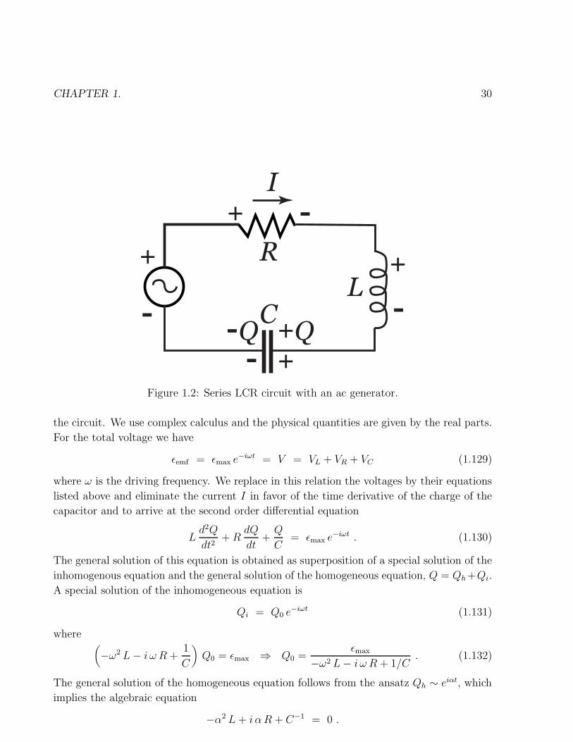
1.3.2 LCR circuit

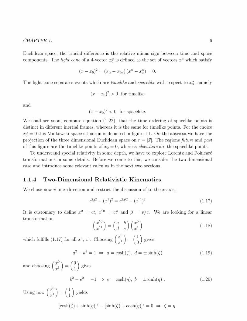
We consider a resistor (R), a capacitor (C) and an inductor (L) in series, see figure 1.2.

Charge conservation implies

IR = IC = IL = I (1.126)

where IR, IC and IL are the currents at the resistor, capacitor and inductor, respectively.

The voltages are related to the currents by the following equations

VR = R I and VC =Q

Cwith

dQ

dt= I (1.127)

where Q(t) is the charge on the capacitor. As inductor we consider an idealized infinitely

long solenoid. The induced (back) electromotive force (voltage over the inductor) is the

derivative of the magnetic flux (1.124)

ǫback = VL =1

c

dΦm

dt= L

dI

dt(1.128)

where the constant L > 0 is called self inductance of the coil. In accordance with Lenz’s law

the induced electromotive ǫback will work against the electromotive force ǫemf which drives

CHAPTER 1. 30

Figure 1.2: Series LCR circuit with an ac generator.

the circuit. We use complex calculus and the physical quantities are given by the real parts.

For the total voltage we have

ǫemf = ǫmax e−iωt = V = VL + VR + VC (1.129)

where ω is the driving frequency. We replace in this relation the voltages by their equations

listed above and eliminate the current I in favor of the time derivative of the charge of the

capacitor and to arrive at the second order differential equation

Ld2Q

dt2+R

dQ

dt+Q

C= ǫmax e

−iωt . (1.130)

The general solution of this equation is obtained as superposition of a special solution of the

inhomogenous equation and the general solution of the homogeneous equation, Q = Qh +Qi.

A special solution of the inhomogeneous equation is

Qi = Q0 e−iωt (1.131)

where(−ω2 L− i ω R+

1

C

)Q0 = ǫmax ⇒ Q0 =

ǫmax

−ω2 L− i ω R+ 1/C. (1.132)

The general solution of the homogeneous equation follows from the ansatz Qh ∼ eiαt, which

implies the algebraic equation

−α2 L+ i αR+ C−1 = 0 .

CHAPTER 1. 31

The solution is

α = iR

2L± ωh with ωh =

√1

LC− R2

4L2(1.133)

and we arrive at the general solution of the homogeneous equation

Qh = A1 e−tR/(2L) e+iωh t + A2 e

−tR/(2L) e−iωh t . (1.134)

Due to the exponential damping the homogeneous solution dies out for large times and we

are left with the inhomogeneous solution Q = Qi (1.131). The homogeneous solution has to

be used for getting the initial values right, e.g. for turning the circuit on or off. In the large

time limit the essential features of the LCR circuit are those of the inhomogeneous solution,

which we investigate now in more details.

For the inhomogeneous solution (1.131) Q0 is a complex constant. To separate the

amplitude of Q0 from its phase we write

Q0 = Qmax e−iδ with Qmax = |Q0| =

ǫmax√(1/C − ω2L)2 + ω2R2

. (1.135)

Following standard conventions, we rewrite the expression for Qmax as

Qmax =ǫmax

ω√

[1/(ω C) − ω L]2 +R2=

ǫmax

ω√

(XC −XL)2 +R2=

ǫmax

ω Z. (1.136)

Here

XC =1

ω Cis called capacitive reactance, (1.137)

XL = ω L is called inductive reactance, (1.138)

and the difference XL −XC is called total reactance. The quantity

Z =√

(XC −XL)2 +R2 is called impedance. (1.139)

Using this notation the original equation (1.132) for Q0 becomes

Q0 =ǫmax

ω (XC −XL − iR)=

ǫmax (XC −XL + i R)

ω Z2. (1.140)

It follows from Q0 = Qmax cos(δ) − i Qmax sin(δ) that the phase δ is given by1

tan δ = − sin(δ)

cos(δ)= −ImQ0

ReQ0=

R

XL −XC. (1.141)

From equation (1.127) we see that VC is in phase with the charge Q

VC =Qmax

Ce−iδ e−iωt (1.142)

1Note that in [8] the phase δ is defined with respect to the current instead of the charge, what leads tothe equation δ = (XL − XC)/R.

CHAPTER 1. 32

and the phase of the current I is shifted by π/2 with respect to VC :

I =dQ

dt= −i ω Qmax e

−iδ e−iωt = ωQmax e−iδ−iπ/2 e−iωt

= Imax e−iδ−iπ/2 e−iωt (1.143)

where we used −i = exp(−iπ/2). Note also that Imax = ωQmax together with equa-

tion (1.136) implies

Imax =ǫmax

Z=

ǫmax√[1/(ω C) − ω L]2 +R2

. (1.144)

The voltage over the resistor is in phase with the current

VR =Imax

Re−iδ−iπ/2 e−iωt (1.145)

whereas the voltage over the inductor is shifted by another π/2 phase factor:

VL = LdI

dt= ω L Imax e

−iδt−iπ eiωt . (1.146)

The current amplitude (1.144) takes its maximum at the resonance frequency

ω0 =1√LC

. (1.147)

Note that Qmax(ω0) = ǫmax/(ω0R) due to equation (1.136). For R 6= 0 the maximum of Qmax

is shifted by an amount of order (R/L)2 away from ω0. We find it by differentiation of Qmax

with respect to ω2:

−2L (C−1 − ω2max L) +R2 = 0 =⇒ ωmax =

√1

LC− R2

2L2. (1.148)

Note, that this ωmax value is lower than the frequency ωh of the damped homogeneous

solution (1.134), while the resonance frequency ω0 is larger.

Bibliography

[1] P.J. Mohr and B.N. Taylor, CODATA Recommended Values of the Fundamental

Physical Constants: 1998, J. of Physical and Chemical Reference Data, to appear.

See the website of the National Institute of Standards and Technology (NIST) at

physics.nist.gov/constants.

[2] A. Einstein, Zur Elektrodynamik bewegter Korper, Annalen der Physik 17 (1905) 891–

921.

[3] A. Einstein, Ist die Tragheit eines Korpers von seinem Energieinhalt abhangig?, Annalen

der Physik 18 (1906) 639–641.

[4] C. Hefele and R. Keating, Science 177 (1972) 166, 168.

[5] J.D. Jackson, Classical Electrodynamics, Second Edition, John Wiley & Sons, 1975.

[6] B.W. Petley, Nature 303 (1983) 373.

[7] W. Rindler, Introduction to Special Relativity, Clarendon Press, Oxford 1982.

[8] P.A. Tipler, Physics for Scientists and Engineers, Worth Publishers, 1995.

[9] R.F.C. Vessot and M.W. Levine, GRG 10 (1979) 181.