Embed Size (px)
Citation preview
Species distribution modelling of stream macroinvertebrates
under climate change scenarios
Dissertation
zur Erlangung des Doktorgrades
der Naturwissenschaften
vorgelegt beim Fachbereich Biowissenschaften
der Johann Wolfgang Goethe -Universität
in Frankfurt am Main
von
Sami Jan-Henrik Domisch
aus Helsinki
Frankfurt am Main (2012)
(D30)

vom Fachbereich Biowissenschaften der Johann Wolfgang Goethe-Universität
als Dissertation angenommen.
Dekanin: Prof. Dr. Anna Starzinski-Powitz
Gutachter: Prof. Dr. Peter Haase und Prof. Dr. Oliver Tackenberg
Datum der Disputation: 29.11.2012

III
Abstract
There is increasing evidence that climate change will have a severe impact on species’
distributions by altering the climatic conditions within their present ranges. Especially
species inhabiting stream ecosystems are expected to be strongly affected due to warm-
ing temperatures and changes in precipitation patterns. The aim of this thesis was to
investigate how distributions of aquatic insects, i.e., benthic stream macroinvertebrates
would be impacted by warming climates. The methods comprised of an ensemble fore-
casting technique based on species distribution models (SDMs) and climate change sce-
narios of the Intergovernmental Panel on Climate Change of the year 2080. Future
model projections were generated for a wide variety of species from a number of taxo-
nomic orders for two spatial scales: a stream network within the lower mountain ranges
of Germany, and the entire territory across Europe. In addition, the effect of the model-
ling technique on habitat suitability projections was investigated by modifying the
choice of study area (continuous area vs. stream network) and the choice of predictors
(standard vs. corrected set).
Projections of future habitat suitability showed that potential climate-change impacts
would be dependent on species’ thermal preferences, and with a similar pattern for both
spatial scales. Future habitat suitability was projected to remain for most or all of the
modelled species, and species were projected to track their climatically suitable condi-
tions by shifting uphill along the river continuum within the lower mountain ranges, and
into a north-easterly direction across Europe. Cold-adapted headwater and high-latitude
species were projected to lose suitable habitats, whereas gains would be expected for
warm-adapted river and low-latitude species along the river continuum and across Eu-
rope, respectively. Additionally, habitat specialist species in terms of endemics of the
Iberian Peninsula were identified as potential climate-change losers, highlighting their
restricted habitat availability and therefore vulnerability to warming climates.
The main findings of this thesis underline the high susceptibility of stream macroinver-
tebrates to ongoing climate change, and give insights into patterns of possible conse-
quences due to changes in species’ habitat suitability. Concerning the methodology, a
clear recommendation can be given for future modelling approaches of stream macroin-
vertebrates by building models within a stream network and with a careful choice of
environmental predictors, to reduce uncertainties and thus to improve model projec-
tions.

IV
Table of contents Abstract ......................................................................................................................... III
List of Figures ................................................................................................................VI
List of Tables................................................................................................................ VII
Abbreviations and Definitions...................................................................................VIII
General Introduction ...................................................................................................... 1
Chapter 1 – Climate-change winners and losers: stream macroinvertebrates
of a submontane region in Central Europe............................................. 7
1.1 Introduction ......................................................................................... 8
1.2 Methods............................................................................................... 9
1.3 Results ............................................................................................... 15
1.4 Discussion ......................................................................................... 17
Chapter 2 – How would climate change affect European stream
macroinvertebrates’ distributions? ....................................................... 23
2.1 Introduction ....................................................................................... 24
2.2 Methods............................................................................................. 25
2.3 Results ............................................................................................... 31
2.4 Discussion ......................................................................................... 36
Chapter 3 – Choice of study area and predictors affect species distribution
models of stream macroinvertebrates .................................................. 40
3.1 Introduction ....................................................................................... 41
3.2 Methods............................................................................................. 43
3.3 Results ............................................................................................... 50
3.4 Discussion ......................................................................................... 53
Summary and general conclusions .............................................................................. 57
Deutschsprachige Zusammenfassung.......................................................................... 62
References ...................................................................................................................... 69

V
Appendices ...................................................................................................................82
Appendix 1...............................................................................................82
Appendix 2...............................................................................................89
Appendix 3...............................................................................................90
Appendix 4...............................................................................................91
Appendix 5.............................................................................................101
Author contributions ...................................................................................................102
Acknowledgements ......................................................................................................103
Erklärungen .................................................................................................................105
Curriculum Vitae.........................................................................................................106

VI
List of Figures
Fig. 1 General work flow of the species distribution modelling procedure...................6
Fig. 1.1 Location of the study area and the stream network ...........................................10
Fig. 1.2 Mean annual air temperatures of species’ occurrences .....................................11
Fig. 1.3 Mean relative contributions of environmental predictors..................................16
Fig. 1.4 Mean altitudes of present and future suitable habitat areas for the
investigated species. ..........................................................................................17
Fig. 1.5 The mean annual air temperature of species’ occurrences correlated with
altitudinal shifts and species range changes......................................................18
Fig. 2.1 Relative changes in the number of species for each grid cell for which
climatically suitable areas were projected under climate warming scenarios...32
Fig. 2.2 Mean annual air temperature of species occurrence plotted against the
changes of climatically suitable areas under climate warming scenarios .........34
Fig. 3.1 Scheme of the four modelling designs...............................................................44
Fig. 3.2 Location of the study area and the stream network ...........................................45
Fig. 3.3 The relative predictor contributions of the final consensus models
for the four modelling designs, averaged over all species. ...............................50
Fig. 3.4 The number of grid cells classified as suitable from the four
modelling designs, averaged over all species....................................................51
Fig. 3.5 Modelled suitable habitats for Aphelocheirus aestivalis (Fabricius, 1794),
Heteroptera, derived from the four modelling designs .....................................52

VII
List of Tables
Table 1.1 Macroinvertebrates used for species distribution models, with the
corresponding taxonomic groups, number of species records,
species range changes and AUC values........................................................ 12
Table 2.1 Comparisons of percent changes, and latitudinal and longitudinal
shifts of climatically suitable areas of endemic/non-endemic,
rare/common and holo-/merolimnic species................................................. 35
Table 2.2 Comparisons of percent changes, and latitudinal and longitudinal
shifts of climatically suitable areas of species grouped for their stream
zonation preference and current preference along the river continuum ....... 35
Table 3.1 The predictors used for calibrating SDMs for the four modelling designs.... 47
Table 3.2 Pairwise differences of grid cells classified as suitable between
the four modelling designs............................................................................ 52

VIII
Abbreviations ANN artificial neural networks
a.s.l. above sea level
AUC area under curve
BEM bioclimatic envelope model
CSA climatically suitable area
CTA classification tree analysis
DEM digital elevation model
FDA flexible discriminant analysis
GAM generalised additive model
GBM gradient boosting machine
GCM global climate model
GLM generalised linear model
IPCC Intergovernmental Panel on Climate Change
SDM species distribution model
SRC species range change
SRE surface range envelope
SRS species range size
TSS true skill statistic
WA weighted average
Definitions
The terms “bioclimatic envelope model” and “species distribution model” refer to the
same modelling technique, however I make a distinction between these two terms based
on the environmental predictors used for modelling:
• “bioclimatic envelope model”: only bioclimatic predictors are used to build the
model
• “species distribution model”: a variety of different types of environmental pre-
dictors, e.g., bioclimatic, topographic, and land use predictors, are used to build
the model.

General Introduction 1
General Introduction
Global climate change is considered to pose – next to habitat destruction, pollution and
species invasions – a major threat to biodiversity (Millennium Ecosystem Assessment,
2005). While climate models predict global mean surface air temperatures to increase
on average by 1.1 – 6.4°C until the end of the 21st century, accompanied by altered pre-
cipitation patterns in terms of the amount and seasonality of precipitation (IPCC, 2007),
climatic isotherms are predicted to shift towards a pole ward direction (Loarie et al.,
2009; Burrows et al., 2011). Organisms may cope with these climatic alterations in two
ways: adapt in terms of phenotypic plasticity (Thackeray et al., 2010), or disperse with
the shifting suitable climatic conditions (Chen et al., 2011). While species are expected
to face huge challenges by adapting to novel climatic conditions in such a short time
frame of ongoing warming climates (Davis, 2001; Hampe & Petit, 2005, but see Hof et
al., 2011), they have been observed to track their climatically suitable conditions in a
northward direction as well as towards higher altitudes (e.g., Parmesan & Yohe, 2003;
Chen et al., 2011). The risk of potential climate-change induced species’ extinctions is
at hand because of limiting dispersal abilities and a potential ‘nowhere to go’ situation
for e.g., high-altitude species (Sala et al., 2000), while possible consequences of spe-
cies’ range shifts on local community structure and species composition remain un-
known. Nevertheless, profound alterations of future biodiversity patterns are expected
for terrestrial, marine and freshwater ecosystems (Pereira et al., 2010; Bellard et al.,
2012).
Freshwater ecosystems cover approximately only 0.8% of the Earth’s surface but con-
tain almost 6% of the described species globally, not to mention their invaluable ecosys-
tem services (Dudgeon et al., 2006). Climate warming is expected to impact freshwater
ecosystems severely by an increased frequency of droughts and floods occurring un-
equally around the globe (Milly et al., 2005; Xenopoulos et al., 2005; IPCC, 2007; Döll
& Zhang, 2010), and the decline in freshwater biodiversity is likely to exceed that of
terrestrial ecosystems (Ricciardi & Rasmussen, 1999; Sala et al., 2000; Bates et al.,
2008). Here, especially streams and rivers are considered highly sensitive to climate
change because they respond stronger to altered runoff patterns than lakes (Poff et al.,
1997; Sala et al., 2000). Species inhabiting stream ecosystems are thus among the most
vulnerable species due to multiple stressors (Ormerod et al., 2010), consisting of warm-
2 General Introduction
ing temperatures accompanied by lowered water oxygen levels, altered flow dynamics,
and additional anthropogenic impacts such as land use changes, chemical loads, and
water withdrawals. Not only that these factors are likely to have an effect on species’
life history characteristics, ultimately resulting in changes in species assemblages (Mul-
holland et al., 1997), they may result in habitat fragmentation and consequently in lim-
ited habitat availability (Sala et al., 2000; Dudgeon et al., 2006; Heino et al., 2009).
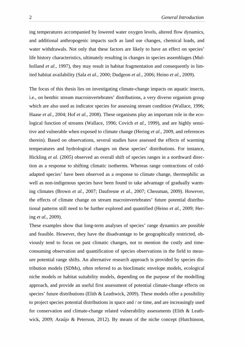
The focus of this thesis lies on investigating climate-change impacts on aquatic insects,
i.e., on benthic stream macroinvertebrates’ distributions, a very diverse organism group
which are also used as indicator species for assessing stream condition (Wallace, 1996;
Haase et al., 2004; Hof et al., 2008). These organisms play an important role in the eco-
logical function of streams (Wallace, 1996; Covich et al., 1999), and are highly sensi-
tive and vulnerable when exposed to climate change (Hering et al., 2009, and references
therein). Based on observations, several studies have assessed the effects of warming
temperatures and hydrological changes on these species’ distributions. For instance,
Hickling et al. (2005) observed an overall shift of species ranges in a northward direc-
tion as a response to shifting climatic isotherms. Whereas range contractions of cold-
adapted species’ have been observed as a response to climate change, thermophilic as
well as non-indigenous species have been found to take advantage of gradually warm-
ing climates (Brown et al., 2007; Daufresne et al., 2007; Chessman, 2009). However,
the effects of climate change on stream macroinvertebrates’ future potential distribu-
tional patterns still need to be further explored and quantified (Heino et al., 2009; Her-
ing et al., 2009).
These examples show that long-term analyses of species’ range dynamics are possible
and feasible. However, they have the disadvantage to be geographically restricted, ob-
viously tend to focus on past climatic changes, not to mention the costly and time-
consuming observation and quantification of species observations in the field to meas-
ure potential range shifts. An alternative research approach is provided by species dis-
tribution models (SDMs), often referred to as bioclimatic envelope models, ecological
niche models or habitat suitability models, depending on the purpose of the modelling
approach, and provide an useful first assessment of potential climate-change effects on
species’ future distributions (Elith & Leathwick, 2009). These models offer a possibility
to project species potential distributions in space and / or time, and are increasingly used
for conservation and climate-change related vulnerability assessments (Elith & Leath-
wick, 2009; Araújo & Peterson, 2012). By means of the niche concept (Hutchinson,

General Introduction 3
1957), these statistical models correlate species’ presences and absences with environ-
mental predictors at those locations to describe a species’ realized niche using model-
ling algorithms, based on the given predictors (a description of the general work-flow of
the modelling procedure in this thesis is given in Box 1 and Fig. 1). As an output, SDMs
provide an extrapolated map of a species’ habitat suitability in geographic space. Next
to obtaining information about the present potential distribution, SDMs can be used to
project future potential distributions based on future environmental predictors to infer
potential thermal refugees under warming climates (Elith & Leathwick, 2009). Here,
SDMs base on the assumption of niche conservatism, i.e., the realized niche of a species
with its biotic interactions remains unchanged over time (Pearman et al., 2008). In addi-
tion, species’ potential abilities regarding adaptation and plasticity in the course of
warming climates are not taken into account (Pearman et al., 2008; Elith & Leathwick,
2009). Despite these rather static assumptions of species’ distributions (Hampe, 2004),
SDMs offer an useful and cost-effective assessment of the potential distribution of spe-
cies (Raxworthy et al., 2003), as well as the impact of climate warming on these poten-
tial distributions (Araújo & Peterson, 2012).
Thus far, SDM-based climate-change analyses on species’ distributional patterns have
been applied for a wide variety of organisms, ranging from plants (e.g., Baselga &
Araújo, 2009; Engler et al., 2011) and terrestrial vertebrates (e.g., Hof et al., 2011; Gar-
cia et al., 2012), to marine organisms (e.g., Robinson et al., 2011), and freshwater fish
(e.g., Buisson et al., 2008; Grenouillet et al., 2010). However, modelling approaches
dealing with the climate-change related vulnerability of stream macroinvertebrates have
begun only recently, and have focused on either single species (e.g., Cordellier & Pfen-
ninger, 2009; Taubmann et al., 2011) or single taxonomic orders (Hof et al., 2012), or
on habitat specialists such as cold-adapted headwater species (Bálint et al., 2011; Sauer
et al., 2011). These results give first insights into the potential vulnerability of stream
macroinvertebrates in terms of possible changes in habitat suitability under climate
change scenarios. However, potential climate-change impacts have not been investi-
gated for a variety of species with, for instance, different thermal adaptations, or spe-
cific habitat requirements and ecological traits (sensu Kotiaho et al., 2005). Moreover,
as the impact of environmental predictors on stream macroinvertebrates is dependent on
the spatial scale (Poff, 1997; Vinson & Hawkins, 1998), the question remains if and
how climate-change effects may occur at different spatial scales for these organisms,
i.e., whether small scale climate-change effects within a mountainous area can be de-

4 General Introduction
tected on a large scale such as Europe, and vice versa sensu Pearson & Dawson (2003)
and Engler et al. (2011). Furthermore, the effect of the modelling procedure itself on
projecting potential distributions of stream macroinvertebrates has not been studied
thoroughly. For instance, the effects of the usage of different study areas on model pro-
jections, such as a continuous area as used in previous studies, or a stream network,
have not been investigated. Similarly, analyses concerning the impact of different pre-
dictors on model performance have been neglected, therefore leaving a gap in the meth-
odology for a proper application of SDMs for this species group.
Outline of the thesis
The objective of this thesis was the application of SDMs on stream macroinvertebrates
with distinct thermal preferences to investigate potential climate-change effects on their
distributions on different spatial scales. For doing so, species’ present distributions were
modelled using SDMs, and subsequently projected into the future by means of two cli-
mate change scenarios of the year 2080 (IPCC, 2007). Further, as SDMs are rather new
tools for assessing climate-change impacts for stream macroinvertebrates, the effects of
different study areas and predictors on model projections were assessed. The thesis con-
sists of the following three studies:
In Chapter 1, the focus lied on a species set consisting of 38 stream macroinvertebrates
inhabiting the lower mountain ranges of Germany. Species were selected according to
their stream zonation preference along the river continuum (Vannote et al., 1980), rang-
ing from cold-adapted headwater species, to generalist and warm-adapted river species.
While cold-adapted species inhabiting mountainous areas are expected to be highly vul-
nerable to warming climates in terms of the predicted summit trap, i.e. a decrease in
available area with increasing altitudes (Thuiller et al., 2005), generalist species may
show an indifferent pattern, whereas warm-adapted river species might take advantage
of the gradual warming of streams (Heino et al., 2009). In particular, the following hy-
pothesis was tested (H1):
• Effects of climate change on the future distributions of stream macroinver-
tebrates along the river continuum are dependent on species’ thermal pref-
erences.
General Introduction 5
In Chapter 2, the modelling extent, i.e., the study area, was expanded to a continental
scale to test whether general patterns of climate-change impacts on species distributions
would persist independently on the spatial scale on which the effects are assessed on. In
this study, the impact of warming climates was simulated for 191 stream macroinverte-
brates’ distributions across Europe. Next to all-species analyses, species were divided
into five ecological and biological trait-based sets to assess the vulnerability of habitat
specialists. Here, the hypothesis was (H2):
• Climatically suitable areas of cold-adapted stream macroinvertebrates and
specialists in terms of specific ecological and biological traits are more
threatened by climate change than those of thermophilic or non-specialist
species across Europe.
Chapter 3 focused on the methodology of SDMs for stream macroinvertebrates. Here,
the objective was to compare the effects of the usage of different study areas and predic-
tors, and how they affect the model statistics and results in terms of the magnitude of
predicted areas classified as suitable for species. Specifically, the study area and the
predictors were altered for four different modelling designs, ranging from a continuous
area to a stream network, and from a non-corrected to a corrected set of predictors.
Models were build for a set of 224 stream macroinvertebrate species across Germany,
and the following hypothesis was tested (H3):
• A stream network as a study area combined with corrected predictors im-
proves the quality of species distributions models for stream macroinverte-
brates by means of model statistics and habitat suitability projections.

6 General Introduction
Box 1 General work flow of the species distribution modelling procedure in this thesis
Species’ geographic records are divided into a training and a testing set, which combined with
present environmental predictors serve as the input data for building the model. The modelling
technique is based on an ensemble forecasting technique using the BIOMOD package in R , i.e.,
several algorithms are combined to reduce uncertainties derived from the usage of different
algorithms (Thuiller et al., 2009). Using a consensus rule based on weighted averages (Marmion
et al., 2009), algorithms providing weak models receive less weight in the final consensus pro-
jection than robust ones. As a next step, this consensus projection delineating the probability of
a species’ present occurrence in geographic space, is converted to a map indicating the presence
and absence of a species using a threshold based on the sensitivity (true positive predictions)
and specificity (true negative predictions, Liu et al., 2005).
To infer the impact of climate change on species’ distributions, the model which was build un-
der present conditions may then be projected into the future using future environmental predic-
tors, such as the future emission scenarios derived from the Intergovernmental Panel on Climate
Change (IPCC, 2007). By combining the map describing the future distribution with the present
one, changes in species’ geographic habitat suitability may be calculated to deduce information
about species’ potential vulnerability under warming climates, their range dynamics in terms of
potential geographic shifts, or potential thermal refugees in the study area.
Figure 1 General work flow of the species distribution modelling procedure in this thesis.
Species presence records (70%)
Species presence records (30%)
Training
Testing
Species distribution modelling algorithms
(BIOMOD / R)
Present environmental predictors
Consensus projection – present (weighted averages)
Present potential distribution (presence / absence)
+
Future environmental predictors (year 2080)
Calculation of e.g. species’ potential - geographic shifts - altitudinal shifts
Consensus projection – 2080 (weighted averages)
Future potential distribution 2080 (presence / absence)
Threshold Threshold

Chapter 1 7
Chapter 1
Climate-change winners and losers: stream macroinvertebrates of a
submontane region in Central Europe
Abstract
Freshwater ecosystems will be profoundly affected by global climate change, especially
those in mountainous areas, which are known to be particularly vulnerable to warming
temperatures. We modelled impacts of climate change on the distribution ranges of 38
species of benthic stream macroinvertebrates from nine macroinvertebrate orders cover-
ing all river zones from the headwaters to large river reaches. Species altitudinal shifts
as well as range changes up to the year 2080 were simulated using the A2a and B2a
Intergovernmental Panel on Climate Change climate-warming scenarios. Presence-only
species distribution models were constructed for a stream network in Germany’s lower
mountain ranges by means of consensus projections of four algorithms, as implemented
in the BIOMOD package in R (GLM, GAM, GBM and ANN). Species were predicted
to shift an average of 122 and 83 m up in altitude along the river continuum by the year
2080 under the A2a and B2a climate-warming scenarios, respectively. No correlation
between altitudinal shifts and mean annual air temperature of species’ occurrence could
be detected. Depending on the climate-warming scenario, most or all (97% for A2a and
100% for B2a) of the macroinvertebrate species investigated were predicted to survive
under climate change in the study area. Ranges were predicted to contract for species
that currently occur in streams with low annual mean air temperatures but expand for
species that inhabit rivers where air temperatures are higher. Our models predict that
novel climate conditions will reorganise species composition and community structure
along the river continuum. Possible effects are discussed, including significant reduc-
tions in population size of headwater species, eventually leading to a loss of genetic
diversity. A shift in river species composition is likely to enhance the establishment of
non-native macroinvertebrates in the lower reaches of the river continuum.
Sami Domisch, Sonja C. Jähnig, Peter Haase (2011). Freshwater Biology 56, 2009–
2020

8 Chapter 1
1.1 Introduction
Freshwater ecosystems will be profoundly affected by global climate change, especially
those in mountainous areas, which are known to be particularly vulnerable to warming
temperatures (Burgmer et al., 2007; Durance & Ormerod, 2007; Hering et al., 2009).
Here, we focus on streams of the lower mountain ranges of Central Europe, which com-
prise the largest mountainous area in Europe and range in altitude up to 1500 m a.s.l.
Streams within this area provide habitats for a wide variety of benthic macroinverte-
brates and are thought to contain the highest level of biodiversity among aquatic macro-
invertebrates in Central Europe outside the Alps (Braukmann, 1987).
The mean temperatures of running waters increase with increasing distance from the
source and, according to the river continuum concept (Vannote et al., 1980), headwater
streams are dominated by cold-adapted species and the lower reaches by thermophilic
species, with a number of generalist species distributed over a wide range along the en-
tire river continuum. In terms of climate change, cold-adapted headwater macroinverte-
brates are likely to experience a loss of thermal refuges because of warming tempera-
tures (Mulholland et al., 1997). Moreover, these species may be progressively replaced
by generalist species taking advantage of the gradual warming of streams, as shown in
long-term data sets by (Daufresne et al., 2007). While river species are expected to
move up in altitude, river warming might additionally facilitate invasion by non-native
macroinvertebrates (Daufresne et al., 2007; Whitehead et al., 2009). A climate change–
driven displacement of species towards higher altitudes will consequently change spe-
cies assemblages at each altitude and therefore result in an altitudinal shift of the river
continuum and lead to a major reorganisation of the species composition and commu-
nity structure of streams (Mouthon & Daufresne, 2006; Burgmer et al., 2007; Daufresne
et al., 2007; Durance & Ormerod, 2007; Haidekker & Hering, 2008).
While these predictions are based on experimental studies as well as long-term data
sets, projections of the impacts of climate change on the ranges of freshwater macroin-
vertebrate species are scarce (Heino et al., 2009). Whereas experimental or case studies
are often geographically restricted, future model projections can consider a larger geo-
graphical region as well as estimate and quantify possible future range shifts under cli-
mate change. Species distributions models (SDMs) are valuable tools for predicting and
evaluating such species range shifts and for following future distributions under climate
change and have been increasingly used in ecology and conservation management (re-
viewed in Elith & Leathwick, 2009). These statistical models use environmental predic-

Chapter 1 9
tors to correlate a species’ geographical distribution with present environmental condi-
tions and produce a probability map of the species’ distribution in geographical space
and time. However, previous distribution-modelling approaches for stream macroinver-
tebrates were based on habitat suitability models (reviewed in Goethals et al., 2007) or
on SDMs covering the whole landscape (Cordellier & Pfenninger, 2009). These land-
scape-based SDMs have the disadvantage of confounding terrestrial and aquatic realms
by using predictors that are not restricted to the stream network but rather to the entire
landscape. Consequently, estimations of species’ ranges remain inaccurate and coarse.
Distributional predictions for aquatic species should therefore take care to not confound
aquatic and terrestrial sites and should include predictors that relate to the stream envi-
ronment as well as climatic predictors. In our approach, we focused on SDMs within a
stream network to limit these erroneous predictions – an approach that, to our knowl-
edge, has been applied so far only to fish (e.g. Buisson et al., 2008).
To assess the responses of stream macroinvertebrates with different thermal tolerances
to climate change, we calculated future distribution ranges under two Intergovernmental
Panel on Climate Change (IPCC) climate-warming scenarios for the year 2080. Follow-
ing the river continuum concept, we selected a set of 38 representative species from
nine macroinvertebrate orders covering all river zones from the source to the large river
reaches. We tested the following hypotheses: (i) as a response to climate change, all
species are predicted to shift towards higher altitudes along the river continuum and (ii)
the distributions of species adapted to different parts of the river continuum will change
in distinct ways. While the suitable habitat area of species from the upper parts of the
river continuum will be reduced by a ‘summit trap effect’ (i.e., a reduction in area with
increasing elevation), the suitable habitat area of species adapted to warmer tempera-
tures from lower parts of the river continuum will increase because of warming tem-
peratures.
1.2 Methods
Study area
The study area covered Germany’s lower mountain range (6°10’–14°90’E, 47°50’–
52°30’N, Fig. 1.1), which is a submontane region with an altitudinal range up to 1,493
m a.s.l. We restricted our analysis to a digitised stream and river network within this
area (LAWA, 2003) because only running waters were considered potential habitats for
the modelled organisms. The running waters ranged from small, coarse, substratum-

10 Chapter 1
dominated highland streams (catchment size 10–100 km2) to large highland rivers
(catchment size 1,000–10,000 km2). In total, the spatial extent of streams and rivers
used for modelling comprised 93,049 grid cells with a spatial resolution of 30 arc sec-
onds (grid cells were ca. 1 km2).
Figure 1.1 (a) Location of the study area in Central Europe. (b) The stream network of the low-er mountain range (grey lines) and all presence records used for modelling (points).
Species data
Because climate change may be perceived differently by species with different thermal
tolerances (‘winners’ and ‘losers’), we selected for analysis species assumed to repre-
sent such different tolerances. However, information on thermal tolerance was not
available for all species. Instead, we considered their stream zonation preference, using
this as a substitute for their temperature range tolerance along the river continuum (sen-
su Vannote et al., 1980). Species’ stream zonation preferences were extracted from a
database that contains information on the autecology of freshwater organisms
(http://www.freshwaterecology.info/, accessed on 25.05.2010, Euro-limpacs Consor-
tium, 2011).
The following species were selected: first, species occurring in the upper reaches (i.e.,
from the eucrenal to the epirhithral, Illies, 1961), with preferences for cooler tempera-
tures (Fig. 1.2, Table 1.1); second, species occurring only in the lower reaches (i.e. from
the hyporhithral to the metapotamal), representing a preference for warmer tempera-
tures; and last, species occurring over a wide range of zones (i.e., within the hypocrenal
and the epipotamal) and thereby exhibiting a broad temperature range preference.
We then searched for species that fulfilled these criteria in three national databases to
retrieve geographical presence records for the SDMs (Umweltbundesamt; Hessisches

Chapter 1 11
Landesamt für Umwelt und Geologie; Landesamt für Umwelt, Messungen und Natur-
schutz Baden-Württemberg, unpublished data). These databases provide stream macro-
invertebrate data from surveys carried out annually in the spring from 2002 to 2008 and
hold a total of 42,576 species presence records from 2,484 sites within our study area.
As a precondition for selection in our study, species needed to have at least 10 presence
records (Stockwell & Peterson, 2002). The databases yielded 38 stream macroinverte-
brates from nine taxonomic groups that fulfilled these criteria, 12 species from the up-
per reaches, 12 species from the lower reaches and 14 species occurring over a wide
range of zones. The selected organisms provided a total of 6564 presence records from
2,151 sites within our study area (Fig. 1.1, Table 1.1).
We then analysed the relationships between the presence records of the selected species
and mean annual air temperature derived from the WorldClim database for the respec-
tive grid cells (http://www.worldclim.org, accessed on 12.03.2010, Hijmans et al.,
2005). Detailed stream temperatures were not available for the entire extent of our study
area. Therefore, we used air temperatures as a surrogate for average stream temperature,
which, except in source zones, tend to be similar to the average air temperature (Caissie,
2006).
Drus
us d
iscol
or
Rhya
coph
ila p
raem
orsa
Rhya
coph
ila pu
besc
ens
Diur
a bica
udat
a
Rheo
crico
topu
s fus
cipes
Eccli
sopt
eryx
dalec
arlic
aLi
thax
nige
r
Leuc
tra br
auer
i
Dino
cras
ceph
alot
es
Pseu
dops
ilopt
eryx
zimm
eri
Drus
us an
nula
tus
Agap
etus f
uscip
es
Caen
is be
skid
ensis
Plec
trocn
emia
gen
icula
ta ge
nicu
lata
Para
lepto
phleb
ia su
bmar
gina
taTo
rleya
maj
or
Hydr
opsy
che f
ulvip
es
Hydr
aena
grac
ilis A
d.
Rhith
roge
na se
mico
lora
taBa
etis r
hoda
ni
Tino
des u
nico
lor
Ancy
lus f
luvia
tilis
Eise
niell
a tetr
aedr
a
Seric
osto
ma fl
avico
rne
Leuc
tra g
enicu
lata
Cheu
mato
psyc
he le
pida
Simu
lium
orna
tum
Lype
redu
cta
Cera
clea
annu
licor
nis
Brac
hyce
ntru
s sub
nubi
lus
Pisid
ium
amni
cum
Neur
eclip
sis bi
macu
lata
Hydr
opsy
che g
utta
ta
Calo
pter
yx sp
lende
ns
Aphe
loch
eirus
aesti
valis
Pisid
ium
supi
num
Gomp
hus v
ulga
tissim
usBa
etis n
exus
Mea
n (±
SD
) ann
ual a
ir te
mpe
ratu
re (°
C)
5
6
7
8
9
10
11
Figure 1.2 Mean (±SD) annual air temperatures of species’ occurrences. Gridded temperature data were derived from the WorldClim dataset.

12 Chapter 1
Table 1.1 Macroinvertebrates used for species distribution models. Species information is pre-sented with the corresponding taxonomic groups, number of species records, species range changes for the year 2080 under the A2a and B2a climate-warming scenarios and AUC values (AUC, area under curve; SRC, species range change; SD, standard deviation; WA, weighted average). The order is equal to that of Fig. 1.2, i.e. according to increasing mean annual air tem-peratures of the species’ occurrences.
Species
Taxonomic
group
Species
records
SRC A2a ±
SD (%)
SRC B2a ±
SD (%)
AUC
(WA)
Drusus discolor (Rambur, 1842) Trichoptera 12 -97.0 ± 1.0 -91.8 ± 0.9 0.99
Rhyacophila praemorsa McLachlan, 1879 Trichoptera 24 -83.1 ± 11.8 -48.3 ± 8.7 0.98
Rhyacophila pubescens Pictet, 1834 Trichoptera 10 -77.5 ± 14.5 -52.9 ± 12.8 0.99
Diura bicaudata (Linnaeus, 1758) Plecoptera 26 -94.7 ± 3.7 -73.0 ± 0.9 0.90
Rheocricotopus fuscipes (Kieffer, 1909) Diptera 13 -100.0 ± 0.0 -96.6 ± 1.8 0.99
Ecclisopteryx dalecarlica Kolenati, 1848 Trichoptera 47 -99.7 ± 0.2 -97.3 ± 0.3 0.95
Lithax niger (Hagen, 1859) Trichoptera 31 -45.1 ± 4.0 -10.8 ± 7.9 0.93
Leuctra braueri Kempny, 1898 Plecoptera 17 -88.4 ± 3.6 -56.8 ± 0.1 0.96
Dinocras cephalotes (Curtis, 1827) Plecoptera 92 34.2 ± 4.9 42.7 ± 10.0 0.95
Pseudopsilopteryx zimmeri (McLachlan, 1876) Trichoptera 16 -98.7 ± 0.9 -36.8 ± 23.2 0.87
Drusus annulatus (Stephens, 1837) Trichoptera 182 -31.0 ± 48.7 37.7 ± 7.5 0.89
Agapetus fuscipes Curtis, 1834 Trichoptera 60 -64.2 ± 23.6 20.5 ± 31.9 0.92
Caenis beskidensis Sowa, 1973 Ephemeroptera 50 -81.2 ± 2.2 -55.3 ± 1.9 0.95
Plectrocnemia geniculata geniculata
McLachlan, 1871
Trichoptera 10 -99.6 ± 0.3 -85.4 ± 5.0 0.97
Paraleptophlebia submarginata (Stephens, 1835) Ephemeroptera 173 -95.4 ± 3.3 -59.7 ± 1.1 0.93
Torleya major (Klapálek, 1905) Ephemeroptera 440 -97.0 ± 2.1 -71.9 ± 1.9 0.85
Hydropsyche fulvipes (Curtis, 1834) Trichoptera 18 15.3 ± 9.4 50.8 ± 7.9 0.95
Hydraena gracilis Ad. Germar, 1824 Coleoptera 66 -93.6 ± 4.5 -73.2 ± 2.3 0.97
Rhithrogena semicolorata (Curtis, 1834) Ephemeroptera 89 16.6 ± 13.6 67.0 ± 20.7 0.95
Baetis rhodani (Pictet, 1843) Ephemeroptera 1766 -27.6 ± 19.1 35.1 ± 18.0 0.79
Tinodes unicolor (Pictet, 1834) Trichoptera 15 -83.9 ± 10.2 -70.6 ± 12.3 0.96
Ancylus fluviatilis O.F. Müller, 1774 Gastropoda 1134 38.9 ± 32.2 106.5 ± 18.6 0.80
Eiseniella tetraedra (Savigny, 1826) Oligochaeta 935 28.5 ± 21.5 104.7 ± 26.4 0.82
Sericostoma flavicorne Schneider, 1845 Trichoptera 57 29.1 ± 71.5 223.2 ± 23.9 0.98
Leuctra geniculata (Stephens, 1836) Plecoptera 168 123.8 ± 90.9 174.3 ± 39.8 0.95
Cheumatopsyche lepida (Pictet, 1834) Trichoptera 133 -95.2 ± 3.0 -75.5 ± 5.7 0.95
Simulium ornatum Meigen, 1818 Diptera 212 244.5 ± 35.0 253.4 ± 3.1 0.90
Lype reducta (Hagen, 1868) Trichoptera 66 -73.0 ± 17.0 64.2 ± 5.9 0.96
Ceraclea annulicornis (Stephens, 1836) Trichoptera 23 552.2 ± 15.3 400.9 ± 23 0.96
Brachycentrus subnubilus Curtis, 1834 Trichoptera 90 94.9 ± 15.8 119.5 ± 8.7 0.98
Pisidium amnicum (O.F. Müller, 1774) Bivalvia 64 -80.8 ± 12.0 -3.0 ± 0.4 0.96
Neureclipsis bimaculata (Linnaeus, 1758) Trichoptera 11 1931.4 ± 109.9 1387.8 ± 102.7 0.91
Hydropsyche guttata Pictet, 1834 Trichoptera 11 949.7 ± 1.0 913.9 ± 30.7 0.94
Calopteryx splendens (Harris, 1782) Odonata 229 403.5 ± 12.4 347.9 ± 7.9 0.93
Aphelocheirus aestivalis (Fabricius, 1794) Plecoptera 197 444.8 ± 13.8 374.8 ± 11.8 0.94
Pisidium supinum Schmidt, 1851 Bivalvia 28 -88.7 ± 6.3 -41.7 ± 6.3 0.99
Gomphus vulgatissimus (Linnaeus, 1758) Odonata 25 720.5 ± 13.9 622.7 ± 17.5 0.94
Baetis nexus Navás, 1918 Ephemeroptera 24 1403.6 ± 21.6 1244.7 ± 21.6 0.99

Chapter 1 13
Environmental predictors
The environmental predictors considered for the SDMs derived from bioclimatic, topog-
raphic and stream-specific categories. From a set of more than 25 predictors, we se-
lected those deemed most relevant for describing the distribution of stream macroinver-
tebrates, with care taken to avoid colinearity among predictors.
Present and future bioclimatic predictors included mean annual air temperature, iso-
thermality (mean diurnal temperature range divided by the annual temperature range),
annual temperature range, annual precipitation and precipitation seasonality (standard
deviation of the weekly precipitation estimates expressed as a percentage of the annual
mean estimates) and were downloaded from the WorldClim database (Hijmans et al.,
2005). The future projections of bioclimatic predictors of the year 2080 were derived
from the global climate models of the Hadley Centre for Climate Prediction and Re-
search (UKMO-HadCM3, Gordon et al., 2000) and the Canadian Centre for Climate
Modelling (CCCMA-CGCM2, Flato et al., 2000). For each, we used the A2a (‘business
as usual’) and B2a (‘moderate’) climate-warming scenarios published by the IPCC
(2007).
We chose slope and aspect as input topographic predictors in the SDMs. Slope is con-
sidered to be an important proxy for flow velocity and oxygen content, whereas aspect
accounts for exposure to sun-induced heating of streams.
Concerning stream-specific predictors, we chose stream type, flow direction and flow
accumulation. Stream type is considered a proxy for stream size, catchment area, ecore-
gion and geology (for a detailed description of German stream types, see http://
www.fliessgewaesser-bewertung.de/en/, Pottgiesser & Sommerhäuser, 2004). Flow
direction is defined as the direction of flow from each cell to its steepest down-slope
neighbour. Flow accumulation is based on the flow direction and defines the number of
cells that flow into each down-slope cell and can thus be seen as a proxy for the drain-
age area (USGS). Both represent flow dynamics in the stream network. The stream-type
layer was derived from (LAWA, 2003), whereas the layers representing slope, aspect,
flow direction and flow accumulation were obtained from a hydrologically corrected
digital elevation model (Hydro1k dataset, http://eros.usgs.gov/, accessed on 07.04.2010,
USGS). All 10 environmental predictors were analysed for colinearity by means of
Pearson correlation coefficients. The predictors were not strongly correlated (-0.7 < r <
0.7, Green, 1979).

14 Chapter 1
Species distribution models
We simulated the distribution of stream macroinvertebrates by means of presence-only
SDMs. Four algorithms consisting of two regression methods (generalised linear mod-
els, GLM and generalised additive models, GAM) and two machine-learning methods
(gradient boosting machine, GBM and artificial neural networks, ANN) were used ac-
cording to the BIOMOD package version 1.1.5 in R (Thuiller et al., 2009; R Develop-
ment Core Team, 2011). Species occurrence data were split into a training set (70%)
and a testing set (30%) by applying a random partition (Araújo et al., 2005). Each algo-
rithm used 5,000 pseudo-absences and a tenfold cross-validation to yield an average
model for each species and algorithm, and prevalence was internally kept constant at 0.5
within the BIOMOD package for all species. These average models, which were cali-
brated under the present conditions, were then projected to the year 2080 using future
bioclimatic predictors from the two global climate models. Non-bioclimatic environ-
mental predictors (i.e., topographic and stream-specific predictors) were kept constant,
as they are considered independent of climate.
Model evaluation was conducted by means of area under curve (AUC) statistics from a
receiver-operating characteristic analysis, which is a threshold-independent evaluation
of model discrimination (Fielding & Bell, 1997). AUC values range from 0.5 to 1,
where 0.5 represents no discrimination and 1 represents perfect discrimination (Hosmer
& Lemeshow, 2000). Araújo et al. (2005) showed that a consensus projection signifi-
cantly improves the predictive accuracy of SDMs. We therefore used a consensus pro-
jection for each species and scenario, with weighted averages (WA) based on the pre-
dictive performance of single-model outputs for each species and algorithm. The rela-
tive importance of each algorithm for the final consensus models was obtained by mul-
tiplying the averaged AUC value by a weight decay of 1.6 (default settings). Finally, the
distribution probability maps of present and future projections were transformed into
binary presence–absence maps by applying a cut-off value that minimises the difference
between sensitivity (true-positive predictions) and specificity (true-negative predictions,
Fielding & Bell, 1997).
Species’ responses to climate change
Binary consensus model outputs were first calculated for each species individually, and
the results of the two global climate models were averaged to yield an A2a and a B2a
2080 climate-warming projection. We then analysed the results for each species by cor-

Chapter 1 15
relating with their mean annual air temperature of occurrence using Spearman rank cor-
relations. One species that was predicted to go extinct and thus lacked future projections
was omitted from these analyses.
Altitudinal shifts in species’ ranges were analysed using the mean altitude of the spe-
cies’ suitable habitat area in their present distribution and the mean altitude of future
suitable habitat area under the A2a and B2a scenarios.
Species’ range changes (SRC) were calculated as the difference between the number of
grid cells gained and lost as a percentage of the number of grid cells presently classified
as suitable habitat. We set no dispersal limitations but rather considered the entire
stream and river network as available area for dispersal. Further, in contrast to relative
range changes, we calculated the differences in species’ range sizes (SRS, i.e., the dif-
ference between the number of present and future grid cells classified as suitable habitat
area).
The relative contributions of environmental predictors demonstrated which predictors
contributed most significantly to the predictions of species’ present distributions. As for
the consensus models, the results of all algorithms were averaged using an identical
weighting factor, thus making the relative contributions of environmental predictors
match the final consensus model for each species.
1.3 Results
Model performance
The overall model performance was good for all species (AUC = 0.94 ± 0.05, weighted
average ± SD, Table 1). For all modelled species, a combination of three bioclimatic
predictors (mean annual temperature, annual precipitation and precipitation seasonality)
made the most substantial contribution (50%) to the present distribution of the species
(Fig. 1.3).
Altitudinal shifts in species’ ranges
The models showed that species were predicted to shift on average 122 and 83 m to-
wards higher altitudes by the year 2080 under the A2a and B2a climate-warming sce-
narios, respectively, generally supporting the stated hypothesis of an altitudinal shift
(Paired t-tests: A2a: t36 = -5.33, P < 0.001; B2a: t37 = -5.82, P < 0.001; Fig. 1.4). Spe-
cies occurring at higher altitudes displayed larger altitudinal shifts (left part of Fig. 1.4)
compared with species occurring at lower altitudes (right part). However, no correlation

16 Chapter 1
could be detected between the mean annual air temperature of occurrence and the alti-
tudinal shifts between the present and future suitable habitat areas (Spearman rank cor-
relation tests: A2a: r = -0.19, P = 0.261; B2a: r = -0.03, P = 0.880, Fig. 1.5a–b).
Mean (± SD) relative contribution (%)
0 10 20 30 40
Flow accumulation
Flow direction
Stream type
Aspect
Slope
Precipitation seasonality
Annual precipitation
Annual temperature range
Isothermality
Mean annual temperature
Figure 1.3 Mean (± SD) relative contributions of environmental predictors for determining the present distributions of macroinvertebrate species. The relative contributions of environmental predictors of all algorithms were averaged using identical weights as for the consensus models and were then averaged for all species.
Species’ range changes and sizes (SRC and SRS)
The models showed that SRC and SRS correlated positively with the mean annual air
temperatures of occurrence from the headwaters to large river reaches under both cli-
mate-warming scenarios (Spearman rank correlation tests: SRC A2a: r = 0.67,
P < 0.001; B2a: r = 0.72, P < 0.001, Fig. 1.5c–d; SRS A2a: r = 0.53, P < 0.001; B2a:
r = 0.66, P < 0.001, data not shown). Generally, species occurring at lower mean annual
air temperatures experienced losses in range size, whereas species occurring at higher
mean annual air temperatures mostly showed pronounced increases in range size.
In general, the overall effects on species range and size changes were stronger under the
A2a scenario (‘business as usual’) than under the B2a (‘moderate’) scenario (Fig. 1.5c–
d, Table 1.1). Of the 38 investigated species, one species (3%) was predicted to go ex-
tinct under the A2a climate-warming scenario (Rheocricotopus fuscipes, Diptera, Table
1.1), while all species were predicted to survive under the B2a scenario.

Chapter 1 17
Drus
us di
scol
or
Rhya
coph
ila pr
aemo
rsa
Rhya
coph
ila pu
besc
ens
Diur
a bica
udat
a
Rheo
crico
topu
s fus
cipes
Eccli
sopt
eryx
dalec
arlic
aLi
thax
nige
r
Leuc
tra br
auer
i
Dino
cras
ceph
alot
es
Pseu
dops
ilopt
eryx
zimm
eri
Drus
us an
nula
tus
Agap
etus f
uscip
es
Caen
is be
skid
ensis
Plec
trocn
emia
geni
cula
ta ge
nicu
lata
Para
lepto
phleb
ia su
bmar
gina
ta
Torle
ya m
ajor
Hydr
opsy
che f
ulvip
es
Hydr
aena
grac
ilis A
d.
Rhith
roge
na se
mico
lora
ta
Baeti
s rho
dani
Tino
des u
nico
lor
Ancy
lus f
luvia
tilis
Eise
niell
a tetr
aedr
a
Seric
osto
ma fl
avico
rne
Leuc
tra ge
nicu
lata
Cheu
mato
psyc
he le
pida
Simu
lium
orna
tum
Lype
redu
cta
Cera
clea a
nnul
icorn
is
Brac
hyce
ntru
s sub
nubi
lus
Pisid
ium
amni
cum
Neur
eclip
sis bi
macu
lata
Hydr
opsy
che g
utta
ta
Calo
pter
yx sp
lende
ns
Aphe
loch
eirus
aesti
valis
Pisid
ium
supi
num
Gomp
hus v
ulga
tissim
usBa
etis n
exus
mea
n al
titud
e (m
a.s.
l.)
0
200
400
600
800
1000
1200
A2aB2aPresent
Figure 1.4 Mean altitudes of present and future suitable habitat areas for the investigated spe-cies under the A2a and B2a climate-warming scenarios.
1.4 Discussion
Model performance and environmental predictors
We obtained good consensus models for each species, giving confidence that the mod-
els will be useful for future attempts to understand possible changes in species’ ranges
driven by climate change. However, two general issues are crucial to bear in mind when
predicting the distributions of stream macroinvertebrates. First, there is a scarcity of
data for the most appropriate predictors, and second, there is a major lack of informa-
tion concerning the ecological preferences of macroinvertebrates (Heino et al., 2009).
One of the most appropriate environmental predictors for which there is a deficiency of
data is stream temperature, which strongly influences the distribution of stream macro-
invertebrates (Haidekker & Hering, 2008) and affects their life history characteristics
and productivity (Mulholland et al., 1997; and references therein). This deficiency par-
ticularly affects species considered as headwater species in the SDMs, a fact that is like-
ly to derive from the use of air temperatures as a surrogate. Temperatures in head-

18 Chapter 1
A2a
6 7 8 9 10 11
Alti
tudi
nal s
hift
(m)
0
200
400
600
6 7 8 9 10 11
Spec
ies r
ange
cha
nges
(%)
0
500
1000
1500
2000
B2a
6 7 8 9 10 11
0
200
400
600
6 7 8 9 10 11
0
500
1000
1500
2000
Mean annual air temperature (°C)
(a) (b)
(c) (d)
Mean annual air temperature (°C) Figure 1.5 The mean annual air temperature of species’ occurrences (compare with Fig. 1.2) correlated with altitudinal shifts (a–b) and species range changes (c–d) under the A2a and B2a climate-warming scenarios.
water streams are strongly influenced by groundwater temperatures, which can be sub-
stantially lower than ambient air temperatures. Consequently, air temperature may be a
poor surrogate for water temperature in these streams, leading to high variability in our
SDMs, which in turn may have resulted in prediction errors for these species. This is
corroborated by the fact that the standard deviations of the mean annual air temperatures
of the species’ occurrences decreased as the temperature increased, (i.e., from the head-
waters to large river reaches, Spearman rank correlation test: r = -0.60, P < 0.001). Al-
though several methods for estimating stream temperatures from air temperatures were
reviewed by Caissie (2006), such estimations are only feasible for single streams or
subcatchments. In contrast, stream temperatures in the mid and lower reaches are
strongly influenced by air temperatures (Vannote & Sweeney, 1980), and the corre-
sponding estimates are thus more likely to be correct.
Little to no information is available on the ecological preferences of the vast majority of
stream macroinvertebrates, such as those regarding temperature and its impact on the
life cycle (Heino et al., 2009; Hering et al., 2009). Furthermore, our limited understand-

Chapter 1 19
ing of dispersal capabilities hinders attempts to make reliable predictions of range
changes. As a consequence, range shifts and expansions of the investigated species are
best viewed as approximations. The true dispersal capabilities of these species are likely
to be lower than the predicted levels. Moreover, the species predicted to experience in-
creases in their suitable habitat areas will encounter new environmental conditions at
their new locations. For example, there are likely to be different patterns of hydrody-
namics and different substrata in the stream bed owing to altered flow patterns, making
reliable predictions of future ranges challenging.
Ecological consequences of species range changes
Our models show that the projected changes in species’ ranges generally depend on the
mean annual air temperature of each species’ current range, although this does not apply
to the altitudinal shifts. The suitable habitat areas of species occurring at higher tem-
peratures were predicted to expand under both climate-warming scenarios and vice
versa.
Our models indicate that the suitable habitat areas of species occurring at lower tem-
peratures (i.e., cold-adapted headwater species) will decrease. Contractions in the suit-
able habitat areas of these species induced by climate warming were recently predicted
by Haidekker & Hering (2008) and Chessman (2009). Likewise, the ability of these
species to survive climate warming at higher altitudes of the lower mountain ranges
under the assumption of unrestricted migration seems probable and has been also pre-
dicted by Wilson et al. (2005) and Burgmer et al. (2007). Thus, the models are corrobo-
rated by findings from previous experimental studies as well as long-term data sets.
However, cold-adapted hololimnic species (with a fully aquatic life cycle) often have
small geographical ranges, poor active dispersal abilities and narrow habitat require-
ments and are considered particularly threatened by climate change (Wilson et al.,
2007). They might, therefore, encounter a ‘nowhere to go’ situation as a result of the
summit trap effect (Thuiller et al., 2005; Bässler et al., 2010). Taking into account that
headwaters can constitute three-quarters or more of the total stream channel length in a
drainage basin (Clarke et al., 2008), the predicted loss of suitable habitat area in such a
large part of the continuum might result in a significant reduction in population size or
even population extinctions. This would inevitably lead to a loss of genetic diversity, as
these species form highly isolated populations in mountainous ecosystems (Clarke et
al., 2008; Lehrian et al., 2009; Taubmann et al., 2011). In small catchment areas, the

20 Chapter 1
genetic diversity might fall below that required to sustain a minimum population size
and thus eventually lead to species extinctions in these areas.
An overall trend towards enlargement of the suitable habitat areas of species occurring
at higher temperatures (i.e., warm-adapted river species) under both climate-warming
scenarios is evident despite the great variability among the investigated species, most
likely reflecting their ecological characteristics (McPherson & Jetz, 2007). Besides the
expansion of these species’ suitable habitat areas into gaps within their present suitable
habitat areas, the models showed that the suitable habitat areas of these species might
extend towards higher elevations along the stream network. However, our modelling
approach did not take evaporative cooling of streams into account, which might con-
strain the rise in stream temperatures. Although the altitude of the stream network used
for modelling ranged from 29 to 1351 m a.s.l., and a wide range of temperatures were
included at each elevation to calibrate the models, the altitudinal shifts of these species
may have been overestimated if temperature-dependent predictors of future climate sce-
narios ranged beyond the present calibration data.
Nonetheless, the warming of the lower reaches of the continuum may in general provide
accessible habitat for non-native species, which may already be adapted to higher tem-
peratures and ⁄ or lower oxygen contents (Daufresne et al., 2007; Rahel & Olden, 2008).
This could lead to major changes in species composition and community structure in the
lower reaches, especially if potential newcomers show characteristics of keystone or
ecosystem engineering species.
Under both climate-warming scenarios, our models suggest that most species will shift
up in altitude along the river continuum. Species in headwater regions were predicted to
lose large amounts of suitable habitat area, while species of the mid and lower reaches
might progressively replace cold-adapted species by taking advantage of the gradual
warming of streams, in agreement with current opinion (Daufresne et al., 2007). Al-
though the models showed that species occurring in river reaches are favoured by
warming temperatures, the question remains open as to whether this will result in less
specialised communities, as previously suggested by Haidekker & Hering (2008).
However, the variable species range changes under the two global climate models indi-
cate that clearly defined predictions are difficult to render. The heavier losses of suitable
habitat areas under the A2a scenario compared with the B2a scenario can probably be
attributed to temperatures increasing beyond the species’ tolerances. For instance, our
study predicted the extinction of the chironomid species Rheocricotopus fuscipes (Dip-

Chapter 1 21
tera) under the A2a scenario (Table 1.1). The annual temperature range (the difference
between the minimum temperature of the coldest period and the maximum temperature
of the warmest period) accounted for 67% of the present distribution of R. fuscipes (re-
sults not shown). In contrast, the same predictor contributed on average only 10% to all
other species (Fig. 1.3). On average, the annual temperature range in our study area will
increase by 3°C under the A2a scenario and by 1.7°C under the B2a scenario. Increases
in the annual temperature range under the A2a scenario could therefore delimit the fu-
ture distributions of certain species.
Implications for mitigation
In general, our models indicate that climate warming will alter the ranges of macroin-
vertebrate species across the river continuum, from the headwaters to the lower reaches.
This raises the question of how climate change-driven effects on the diversity of stream
macroinvertebrates in the lower mountain ranges might be mitigated. Vulnerable macro-
invertebrates might possibly be conserved by reducing interacting stressors, either di-
rectly (e.g., reduction in chemical loads and contamination) or indirectly (e.g., land use
changes). Furthermore, the establishment and maintenance of dispersal corridors and
dispersal networks in protected areas should be enacted to especially if potential new-
comers show characteristics of keystone or ecosystem engineering species.
Under both climate-warming scenarios, our models suggest that most species will shift
up in altitude conserve minimum viable populations (Heino et al., 2009). For this pur-
pose, there is, however, a clear need for information on the dispersal abilities of differ-
ent species (Kappes & Haase, 2011) and for SDMs that account for this factor. For mer-
olimnic invertebrates (species with an aquatic larval and a terrestrial adult stage) in par-
ticular, we propose a two-model solution that does not confound aerial and aquatic pre-
dictors. The aquatic stage of these species is modelled with predictors that are important
for describing the larval phase (aquatic stage model), whereas the adult stage is mod-
elled with predictors that are important for describing the aerial stage (aerial stage mod-
el). The results of these two models are then combined to further improve estimations of
dispersal. Moreover, predictions for especially cold-adapted hololimnic species (fully
aquatic life cycle) could be improved by using more relevant predictors for these spe-
cies, such as water temperatures at a fine scale (<1 km2).
This study sheds light onto possible impacts of climate change on the ranges of selected
species along the river continuum in streams of a mountainous ecosystem. Our stated

22 Chapter 1
predictions that climate change will have differential impacts on stream macroinverte-
brates with different thermal tolerances were corroborated by the SDM runs. In addi-
tion, the results showed that the SDMs of macroinvertebrates within stream networks
are useful for predicting possible shifts in species’ ranges. Further investigations are
required to understand the direct and indirect impacts of climate change and its interac-
tions with other stressors on stream macroinvertebrates.

Chapter 2 23
Chapter 2
How would climate change affect European stream macro-
invertebrates’ distributions?
Abstract
Climate change is predicted to have profound effects on freshwater organisms due to
warming temperatures and altered precipitation patterns, that will affect the distribution
of species climatically suitable areas. We modelled the future climatic suitability for
191 stream macroinvertebrate species from 12 orders across Europe under two climate
change scenarios for 2080 using an ensemble of bioclimatic envelope models (BEMs).
Analyses included assessments of relative changes in species’ climatically suitable areas
as well as their potential shifts in latitude and longitude with respect to species’ thermal
preferences. Additionally, the effects of climate change on species were analysed by
subdividing them into the following ecological and biological trait-based sets: 1) en-
demic / non-endemic and 2) rare / common species within European ecoregions; 3) spe-
cies with an aquatic larval and a terrestrial adult stage / species with a fully aquatic life
cycle; and species based on their 4) stream zonation preference and 5) current prefer-
ence. Suitable climates in the future were projected to remain in Europe for nearly 99%
of the modelled species under both scenarios. Nevertheless, BEMs projected a decrease
of climatically suitable areas for 57-59% of the species depending on the scenario. Cli-
matically suitable areas were projected to shift on average 4.7-6.6° northward and 3.9-
5.4° eastwards. Cold-adapted and high-latitude species were projected to lose climati-
cally suitable areas, while gains were expected for warm-adapted and low-latitude spe-
cies. Endemic species of the Iberian-Macaronesian region were an exception. Even un-
der the assumption of unlimited dispersal these thermophilic species were projected to
lose significantly higher amounts of climatically suitable areas than non-endemic spe-
cies, whereas no significant differences in changes of climatically suitable areas could
be observed for other trait-based sets. Modelled shifts of climatically suitable areas thus
underpin the high vulnerability of freshwater organisms to ongoing climate change.
Sami Domisch, Miguel B. Araújo, Núria Bonada, Steffen U. Pauls, Sonja C. Jähnig,
Peter Haase. Submitted to Global Change Biology

24 Chapter 2
2.1 Introduction
Europe harbours a great diversity of stream macroinvertebrates (see e.g., Hof et al.,
2008), which are highly sensitive and vulnerable when exposed to climate change (Her-
ing et al., 2009 and references therein). Climate change will impose severe challenges
for stream biota across Europe due to warming temperatures in northern Europe, in-
creasing risks for flood events in temperate regions, and an increasing frequency of
droughts in southern Europe (IPCC, 2007). Specifically, predicted climate-change im-
pacts on the distribution of stream macroinvertebrates include a reduction of habitat for
cold-adapted species in high latitudes and altitudes (Bálint et al., 2011), as well as for
Southern European (endemic) species (Ribera & Vogler, 2004; Bonada et al., 2009),
habitat specialists (Kotiaho et al., 2005), and species with specialized life history traits
(Hering et al., 2009).
Thus far, assessments on possible climate-change effects, describing the potential fate
of stream macroinvertebrates under warming climates on a continental scale, have fo-
cused either on single species (e.g., Taubmann et al., 2011) or taxonomic orders (Hof et
al., 2012), on cold-adapted headwater species (Bálint et al., 2011), or using expert
knowledge and the categorisation of single taxonomic orders according to their potential
vulnerability (Hering et al., 2009; de Figueroa et al., 2010). To our knowledge no study
has yet assessed possible alterations in terms of species potential distributions for a wide
variety of stream macroinvertebrates using bioclimatic envelope models (BEMs). These
statistical models have proven to be valuable tools in conservation and climate-change
analyses by projecting species habitat suitability in space and/or time, based on climatic
predictors (Elith & Leathwick, 2009; Araújo & Peterson, 2012, and references therein).
While small scale modelling analyses within mountainous regions (Domisch et al.
2011) corroborate observed responses to warming climates for species along the river
continuum (Daufresne et al., 2004; Chessman, 2009), the use of different spatial extents
and resolutions for modelling studies is likely to result in different patterns of species
responses (see e.g., Engler et al., 2011), based on methodological biases rather than
differences in species sensitivities and responses to changing climate conditions. On a
continental scale, a particular challenge for modelling stream macroinvertebrates is to
compile a reliable and comprehensive set of range-wide species records for building
BEMs (Sánchez-Fernández et al., 2008), since models are highly sensitive to the quality
of species distributional data (Barbet-Massin et al., 2010).

Chapter 2 25
We carried out an extensive search for species records to limit the impacts of using in-
complete distributional data. Following a thorough data quality program, we modelled
the present and future climatically suitable areas for 191 species across Europe. We ana-
lysed relative changes in species’ climatically suitable areas as well as their potential
shifts in latitude and longitude with respect to species’ thermal preferences. Addition-
ally, the effects of climate change on species were analysed by subdividing them into
the following ecological and biological trait-based sets: 1) endemic / non-endemic spe-
cies and 2) rare / common species within European ecoregions; 3) species with an
aquatic larval and a terrestrial adult stage / species with a fully aquatic life cycle; and
species groups based on their 4) stream zonation preference and 5) current preference.
We hypothesized that climatically suitable areas would shift northwards due to warming
temperatures (Chen et al., 2011), and that the extent of climate-change effects would be
dependent on species thermal preferences (Domisch et al., 2011). Further, we expected
that endemic and rare species would be more threatened by warming climates than the
respective counterparts, as specific habitat requirements may not be present under future
climate conditions (Malcolm et al., 2006; IPCC, 2007). Similarly we expected that spe-
cies with a fully aquatic life cycle would lose more climatically suitable area than spe-
cies with an aquatic larval and terrestrial adult stage, as changing precipitation patterns
may force the restriction of habitat availability (Xenopoulos et al., 2005). Since species
occurring at specific stream zones along the river continuum are expected to respond
differentially to climate change due to different thermal regimes (Hering et al., 2009;
Domisch et al., 2011), we expected that cold-adapted headwater species would be more
vulnerable to warming climates than thermophilic species distributed along the mid- and
lower-reaches of the river continuum. Last, climate warming is expected to result in
changes in water availability as well as in stream discharge changes (Milly et al., 2005;
Xenopoulos et al., 2005), and we hypothesized that climatically suitable areas for spe-
cies adapted to fast running waters would decrease because of expected droughts and
alterations in stream flow (Bonada et al., 2007b).
2.2 Methods
Study area
BEMs were set up for the extent of Europe including Iceland (24°W–52°E longitude
and 33°–72°N latitude) with a spatial resolution of 5´ (approximately 10 km2). The large
extent (including parts of Northern Africa and Middle East) was chosen to overcome the

26 Chapter 2
limitation of using truncated environmental gradients for calibrating models within spe-
cies’ known ranges (Thuiller et al., 2004). Moreover, this procedure minimises the con-
straints of non-analogue climates on the predictive model performance for projecting
climatic suitability under future climate scenarios (Fitzpatrick & Hargrove, 2009).
Species data
Thorough criteria were used to select the species included in the study, as several stud-
ies have shown the limitation of poor quality species’ records (i.e., incomplete distribu-
tional data) on the predictive performance of BEMs (Araújo & Guisan, 2006; Barbet-
Massin et al., 2010; Sánchez-Fernández et al., 2011).
We compiled a set of geographic records across Europe for 1733 stream macroinverte-
brate species from data collected by taxonomists. These records were sourced from the
EU-funded STAR project (Furse et al., 2006), the GUADALMED projects and an In-
ternational Cooperation project with Morocco (Bonada et al., 2004; Bonada et al.,
2008), collection material from S.U. Pauls and data digitized for Portugal by M.B.
Araújo (Terra, 1994).
Furthermore, we considered data compiled by the Swedish University of Agricultural
Sciences (www.slu.se, accessed on 26.09.2011), three national databases (Umwelt-
bundesamt; Hessisches Landesamt für Umwelt und Geologie; and Landesamt für Um-
welt, Messungen und Naturschutz Baden-Württemberg, unpublished data), the SeSam
database of the Senckenberg Museum (http://sesam.senckenberg.de, accessed on
30.09.2011), the ZOBODAT database (www.zobodat.at, accessed on 28.09.2011), and
the Global Biodiversity Information Facility database (www.gbif.org, accessed on
22.09.2011) as additional data sources to retrieve presence records for species listed in
our set. For public databases, only records were retrieved which were published by nat-
ural history museums or research facilities, where the resolution of records was not
coarser than that of our models, and where terms of use allowed the usage of data. His-
toric occurrences recorded earlier than 1950 were discarded, as the climatic baseline for
modelling ranged from 1950 to 2000. After scanning these databases for species listed
in our initial species set, records were resampled to a 5´ grid resolution, and species
needed to occupy at least 15 grid cells while duplicate records of a single species falling
into one grid cell were omitted. This criterion was fulfilled for 986 species.
We then checked for a geographic bias of these records and investigated, how well spe-
cies records represented the known species ranges by using the classification of Euro-

Chapter 2 27
pean ecoregions as a reference (Illies, 1978) by means of a digitised map
(http://www.eea.europa.eu/data-and-maps/figures/ecoregions-for-rivers-and-lakes, ac-
cessed on 28.09.2011, EEA, 2011). Here, records for each species needed to be present
in at least two out of three ecoregions where the species is known to occur (described in
Limnofauna Europaea, Andrássy et al., 1967) and the freshwaterecology.info database
(http://www.freshwaterecology.info/, accessed on 28.09.2011, Euro-limpacs Consor-
tium, 2011; Schmidt-Kloiber & Hering, 2012). This procedure resulted in discarding the
vast majority of species with highly incomplete records. In total, our final species list
used for BEMs comprised 191 species from 12 macroinvertebrate orders. Species re-
cords ranged from Morocco to arctic Norway, covered 23 out of 25 European ecore-
gions (all but Iceland and the Caspic depression), and in some species also included
North Africa and the Middle East. The ranges of individual species covered one (i.e.,
endemic) to 24 ecoregions (widespread species, see Appendix 1). The match between
the distributional data (i.e., species records) and their known ranges (i.e., ecoregions)
was on average 81 ± 13% (mean ± standard deviation).
Climate data
To build the BEMs, we chose climatic predictors that characterize energy and water
regimes (Whittaker et al. 2007): mean annual air temperature (°C), sum of annual pre-
cipitation (mm), and precipitation seasonality (coefficient of variation). Though these
predictors correspond to a small subset of available variables they have been success-
fully used for modelling stream macroinvertebrates on a continental scale (e.g., Taub-
mann et al., 2011; Hof et al., 2012) as well as plants (e.g., Baselga & Araújo, 2009;
Engler et al., 2011) and many vertebrate taxa (e.g., Garcia et al., 2012; Hof et al.,
2011). Climatic predictors for the present, from here on referred to as the ‘baseline’
from 1950-2000, were retrieved from the WorldClim dataset in a 5´ grid resolution
(www.worldclim.org, accessed on 01.08.2011, Hijmans et al. 2005). Bioclimatic predic-
tors for the future, averaged across 2070-2099 (hereafter referred to as ‘2080’), were
obtained from the CIAT database (www.ccafs-climate.org, accessed on 01.08.2011,
Ramirez & Jarvis, 2008) and from four global climate models (GCMs): HCCPR
HADCM3 (Gordon et al., 2000), CCCMA-CGCM2 (Flato et al., 2000), CSIRO-MK2
(Gordon et al., 2002), and NIES99 (Emori et al., 1999). For each, we used the A2a and
B2a climate warming scenario of the 4th Assessment Report of the Intergovernmental
Panel on Climate Change (IPCC, 2007), respectively. The A2a scenario is referred to as

28 Chapter 2
the ‘extreme’ scenario with a projected warming of the mean annual temperature of 5.8
± 1.3°C, whereas the B2a scenario reflects a ‘moderate’ scenario with a projected mean
annual temperature increase of 4.4 ± 1.0°C in our study area (± standard deviation).
Uncertainties deriving from novel future climatic conditions in our study area were as-
sessed by calculating non-analogue climates for each GCM.
Bioclimatic envelope modelling
We fitted BEMs using an ensemble forecasting framework (Araújo & New, 2007) based
on seven algorithms as implemented in the BIOMOD package version 1.1.7 in R (gen-
eralised linear models, GLM; generalised additive models, GAM; gradient boosting
machine, GBM; flexible discriminant analysis, FDA; classification tree analysis, CTA;
artificial neural networks, ANN; surface range envelopes, SRE; Thuiller et al., 2009; R
Development Core Team, 2011). Models were calibrated using climate predictors for
the baseline period after species presence records were randomly split into a training set
(70%) and a testing set (30%, Fielding & Bell, 1997; Araújo et al., 2009). Each algo-
rithm used 10,000 pseudo-absences and a tenfold cross validation which yielded an av-
erage model for each species and algorithm. Model evaluation based on the true skill
statistic (TSS), which has been shown to be superior in measuring the performance of
BEMs when the predictions are expressed in presence-absence maps (Allouche et al.,
2006). TSS scores incorporate sensitivity (true positive predictions) and specificity (true
negative predictions) and range from 0 to 1, where 0 describes a model no better than
random while 1 describes a perfect agreement with the model and species’ records. To
reduce uncertainties derived from different modelling algorithms, single algorithm re-
sults for each species were averaged to a consensus model based on model performance
(TSS, see also Araújo et al., 2011). Here, a weight decay of 1.6 was used, while only
models performing better that TSS > 0.4 were used in the consensus, discarding weak
models from the consensus model (e.g., Araújo et al., 2011; Engler et al., 2011). At
least two algorithms were required to yield a TSS score higher than 0.4, otherwise no
consensus model was created, and the respective species was removed from further
analyses.
The consensus models were then projected on the entire study area for the baseline and
future scenarios. Inter-model variability was handled by averaging consensus projec-
tions of each GCM within a single A2a and B2a scenario. Maps indicating the probabil-
ity of climatic suitability under present and future projections were transformed into
Chapter 2 29
binary presence-absence maps by applying a cut-off value which minimises the differ-
ence between sensitivity and specificity (Liu et al., 2005).
Climate change effects on species
All-species analyses
First, we tested for percent changes in climatically suitable areas between present and
future projections, incorporating the relative number of grid cells lost, kept stable and
gained. Species were identified as either climate-change losers or winners, depending
on a species’ overall loss or gain of climatically suitable area, respectively.
Further, we tested for an overall geographic shift of species’ climatically suitable areas,
and analysed whether the arithmetic mean of the modelled latitude and longitude of the
present climatically suitable areas differed from those of the future by means of paired
t-tests.
To test whether climate-change effects on species climate suitability across their ranges
were related with their thermal preferences, we correlated percent changes of climati-
cally suitable areas, and the latitudinal and longitudinal shifts against the mean tempera-
ture of occurrence. A shift was defined as the difference between present and future
projections in terms of grid cells classified as climatically suitable, with shifts in a
northward and eastward direction as positive, and shifts in a southward and westward
direction as negative, respectively.
Analyses by trait-based sets
We were further interested in climate-change effects of species based on specific bio-
logical and ecological trait-based sets (sensu Kotiaho et al., 2005). We created five sub-
sets, based on the classification in the freshwaterecology.info database (Euro-limpacs
Consortium, 2011; Schmidt-Kloiber & Hering, 2012), and tested for the differences in
shifts between species matching the given criterion versus those which explicitly did
not. Species not classified under specific criteria were omitted from the analyses.
First, we divided species into endemic (species present only in one ecoregion, n = 24)
and non-endemic species (n = 167). Eighty-eight percent of the endemics occurred in
the Iberian-Macaronesion region, while the remaining 12% occurred in the Alps.
Second, we divided a total of 187 species upon their classification for being either rare
(n = 26) or common (n = 161). Rare species may be located in several ecoregions, hav-
ing a wide continental distribution, but tolerate narrow habitat requirements and are

30 Chapter 2
therefore restricted to specific habitats within the ecoregions similar to endemic species
(sensu Mills & Schwartz, 2005).
Third, we divided our species set into merolimnic (i.e., species with aquatic larval and
aerial adult stages, n = 176) and hololimnic (i.e., species with a fully aquatic life cycle,
n = 15), since species with contrasting life cycles are likely to respond differentially to
climate change due to restricted habitat availability under changing precipitation pat-
terns (sensu Xenopoulos et al., 2005).
A fourth subdivision based on species’ stream zonation preferences (n = 73). Species
were classified as headwater species (coded with five or more points for ‘eucrenal’ and
‘hypocrenal’ in the database, n = 34, Hering et al., 2009), or as downstream river spe-
cies (species occurring between the ‘epipotamal’ and ‘hypopotamal’, n = 17). Generalist
species were those occurring over a wide range of the river continuum (present in each
zone within the ‘hypocrenal’ to ‘epipotamal’, n = 22).
Species’ current preference was considered as a fifth criterion for a subdivision (n = 77).
Species were coded for their preference for calm (limnophilic) to fast running waters
(rheobiontic), and classified as limnophilic (n = 8), limno- to rheophilic n = 18), rheo- to
limnophilic (n = 39), rheophilic (n = 77), rheobionts (n = 20), or as indifferent species
(n = 6).
For further details on these subdivisions and classifications, see Hering et al. (2009), de
Figueroa et al. (2010), Euro-limpacs Consortium (2011) and Schmidt-Kloiber & Hering
(2012). Species subsets 1-3 were analysed using Student’s t-tests, and homogeneity of
variances was confirmed with Levene’s tests. In case of highly unbalanced sample siz-
es, Man-Whitney-U tests were computed additionally. Since results did not differ be-
tween the two tests, we show only results from Student’s t-tests to keep analyses fixed.
Climate change effects for subsets 4-5 were analysed using nonparametric Kruskal-
Wallis tests because of unbalanced sample sizes. Future climatically suitable areas were
expected to vanish for two and one species under the A2a and B2a warming scenario,
respectively, and these were thus removed from analyses concerning geographic shifts.

Chapter 2 31
2.3 Results
Model performance
Model performance was high, with average TSS scores of 0.96 ± 0.03 (mean ± standard
deviation, Appendix 1), and consensus projections were created for all of our 191 spe-
cies. Analyses of climate projections revealed that non-analogue climates were re-
stricted to parts of North Africa and the Middle East for all four GCMs, and to a minor
part of the Iberian Peninsula for the HADCM and the NIES climate projections (Ap-
pendix 2).
All-species analyses
On average, the 191 modelled species were projected to lose climatically suitable area
by 2.9 ± 66.0% and 1.2 ± 54.7% under the A2a and B2a scenario, respectively. From
these, a total of 112 (59%) and 109 (57%) species were projected to lose climatically
suitable area under the A2a and B2a scenarios, respectively. Climate-change loser spe-
cies were projected to lose on average 44.0 ± 29.8% and 38.1 ± 27.0%, whereas winner
species were projected to gain on average 55.4 ± 59.1% and 47.7 ± 42.0% of climati-
cally suitable area under the two scenarios, respectively. Two species were projected to
lose their entire climatically suitable area under the A2a (Oxycera morrisii and Ortho-
cladius holsatus, Diptera) and the B2a scenario (only O. holsatus). Species’ climatically
suitable areas were projected to shift significantly northwards (6.6 ± 2.5° and 4.7 ± 2.2°
under the A2a and B2a scenarios, respectively; paired t-tests: A2a: t188 = -36.58, P <
0.001; B2a: t189 = -29.80, P < 0.001, Fig. 2.1a,b). Similarly, climatically suitable areas
were projected to shift significantly eastwards by 5.4 ± 8.8° and 3.9 ± 6.5° under the
two scenarios, respectively (Paired t-test: A2a: t188 = -8.40, p < 0.001; B2a: t189 = -8.27,
P < 0.001, Fig 2.1a,b).
Percent changes in climatically suitable areas were positively correlated with species’
mean temperature of occurrence under both climate warming scenarios (Pearson corre-
lation coefficients, A2a: r = 0.27, P < 0.001; B2a: r = 0.29, P < 0.001, Fig. 2.2a,b).
Species’ mean temperature of occurrence correlated negatively with projected latitu-
dinal shifts of climatically suitable areas under the two scenarios, while no significant
correlation could be found for longitudinal shifts (Pearson correlation coefficients, lati-
tude: A2a: r = -0.29, p < 0.001; B2a: r = -0.33, P < 0.001, longitude: A2a: r = -0.01,
P = 0.895, B2a: r= -0.01, P = 0.831).

32 Chapter 2
Change in species richness (%)
-100 – -76 -75 – -51 -50 – -26 -25 – -1 0 1 – 25 26 – 50 51 – 75 76 – 100 >100
(a)
(b)
Figure 2.1 Relative changes in the number of species for each grid cell for which climatically suitable areas were projected under the A2a (a) and the B2a (b) climate warming scenarios compared to the baseline.
Analyses by trait-based sets
In total, 83% and 79% of the endemic species and 55% and 56% of the non-endemic
species were identified as climate-change losers under the A2a and B2a scenario, re-
spectively. On average, endemic species lost significantly more climatically suitable
areas than non-endemic species (Table 2.1). Similarly, climatically suitable areas of
non-endemic species were projected to shift significantly stronger into a north-easterly
direction, while only a minor northward but a westward shift was observed for endemic

Chapter 2 33
species’ climatically suitable areas under the A2a and B2a scenario, respectively (Table
2.1).
Fifty-five percent and 58% of the rare species were projected to lose climatically suit-
able areas under the two scenarios, while 59% and 57% of the common species were
projected to lose climatically suitable areas under the two scenarios, respectively. Cli-
matically suitable areas of rare species were projected to shift on average one degree
more northwards, and on average more than two times further eastwards than those of
common species under both climate warming scenarios, while no significant differences
in shifts regarding percent changes in climatically suitable areas were found (Table 2.1).
The ratio of hololimnic climate-change loser species was 53% and 60%, while 59% and
57% of the merolimnic species were projected to lose climatically suitable areas under
the two scenarios. Climatically suitable areas of hololimnic species were projected to
shift on average 5.3° more eastwards than merolimnic species under the A2a scenario
(Table 2.1). No significant shifts in longitude were projected under the B2a scenario,
nor were shifts in latitude or percent changes in climatically suitable areas significantly
different between holo- and merolimnic species.
Species mean temperature of occurrence was significantly lower for headwater than for
river species, but not significantly different from the mean temperature of occurrence
for generalist species (Kruskal-Wallis test: H2 = 6.48, P = 0.039). On average, 75%,
52% and 53% of the headwater, generalist and river species lost climatically suitable
areas under the A2a scenario, respectively, while 72%, 71%, and 41% of the respective
groups were predicted to lose climatically suitable areas under the B2a scenario. Con-
sidering the average distance, climatically suitable areas of generalist species were pro-
jected to shift significantly more northwards than those of headwater and river species
under both climate warming scenarios (Table 2.2, Kruskal-Wallis test: A2a: H2 = 11.49,
P = 0.003, B2a: Kruskal-Wallis test: H2 =13.11, P = 0.014). Eastwards shifts of climati-
cally suitable areas were on average almost 8 times higher for generalist species than for
headwater species under the two scenarios, respectively (Kruskal-Wallis test: A2a:
H2 =16.49, P = 0.003, B2a: Kruskal-Wallis test: H2 = 19.93, P < 0.001). No significant
differences in percent changes of climatically suitable areas could be observed (Krus-
kal-Wallis test: A2a: H2 = 3.47, p = 0.177, B2a: H2 = 2.89, P = 0.235).
BEMs showed a non-significant tendency in decreasing losses of climatically suitable
areas from calm to fast running waters (Table 2.2). Further, no significant differences in
latitudinal or longitudinal shifts of projected climatically suitable areas could be de-
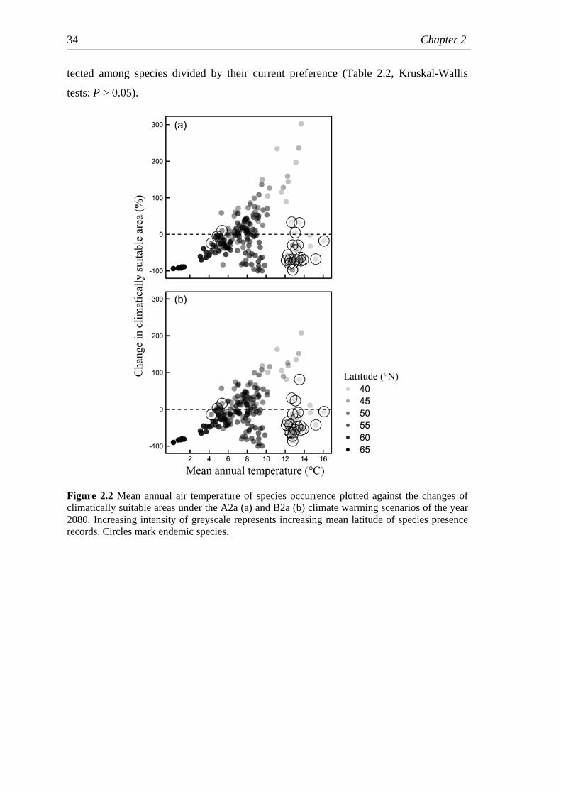
34 Chapter 2
tected among species divided by their current preference (Table 2.2, Kruskal-Wallis
tests: P > 0.05).
Figure 2.2 Mean annual air temperature of species occurrence plotted against the changes of climatically suitable areas under the A2a (a) and B2a (b) climate warming scenarios of the year 2080. Increasing intensity of greyscale represents increasing mean latitude of species presence records. Circles mark endemic species.
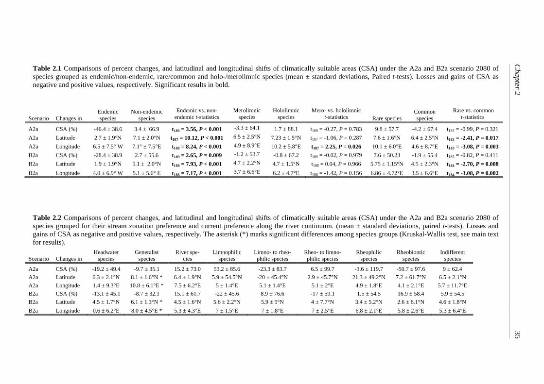
Table 2.1 Comparisons of percent changes, and latitudinal and longitudinal shifts of climatically suitable areas (CSA) under the A2a and B2a scenario 2080 of species grouped as endemic/non-endemic, rare/common and holo-/merolimnic species (mean ± standard deviations, Paired t-tests). Losses and gains of CSA as negative and positive values, respectively. Significant results in bold.
Scenario Changes in Endemic species
Non-endemic species
Endemic vs. non-endemic t-statistics
Merolimnic species
Hololimnic species
Mero- vs. hololimnic t-statistics Rare species
Common species
Rare vs. common t-statistics
A2a CSA (%) -46.4 ± 38.6 3.4 ± 66.9 t189 = 3.56, P < 0.001 -3.3 ± 64.1 1.7 ± 88.1 t189 = -0.27, P = 0.783 9.8 ± 57.7 -4.2 ± 67.4 t185 = -0.99, P = 0.321 A2a Latitude 2.7 ± 1.9°N 7.1 ± 2.0°N t187 = 10.12, P < 0.001 6.5 ± 2.5°N 7.23 ± 1.5°N t187 = -1.06, P = 0.287 7.6 ± 1.6°N 6.4 ± 2.5°N t183 = -2.41, P = 0.017 A2a Longitude 6.5 ± 7.5° W 7.1° ± 7.5°E t188 = 8.24, P < 0.001 4.9 ± 8.9°E 10.2 ± 5.8°E t187 = 2.25, P = 0.026 10.1 ± 6.0°E 4.6 ± 8.7°E t183 = -3.08, P = 0.003 B2a CSA (%) -28.4 ± 38.9 2.7 ± 55.6 t189 = 2.65, P = 0.009 -1.2 ± 53.7 -0.8 ± 67.2 t189 = -0.02, P = 0.979 7.6 ± 50.23 -1.9 ± 55.4 t185 = -0.82, P = 0.411 B2a Latitude 1.9 ± 1.9°N 5.1 ± 2.0°N t188 = 7.93, P < 0.001 4.7 ± 2.2°N 4.7 ± 1.5°N t188 = 0.04, P = 0.966 5.75 ± 1.15°N 4.5 ± 2.3°N t184 = -2.70, P = 0.008 B2a Longitude 4.0 ± 6.9° W 5.1 ± 5.6° E t188 = 7.17, P < 0.001 3.7 ± 6.6°E 6.2 ± 4.7°E t188 = -1.42, P = 0.156 6.86 ± 4.72°E 3.5 ± 6.6°E t184 = -3.08, P = 0.002
Table 2.2 Comparisons of percent changes, and latitudinal and longitudinal shifts of climatically suitable areas (CSA) under the A2a and B2a scenario 2080 of species grouped for their stream zonation preference and current preference along the river continuum. (mean ± standard deviations, paired t-tests). Losses and gains of CSA as negative and positive values, respectively. The asterisk (*) marks significant differences among species groups (Kruskal-Wallis test, see main text for results).
Scenario Changes in Headwater
species Generalist
species River spe-
cies Limnophilic
species Limno- to rheo-philic species
Rheo- to limno-philic species
Rheophilic species
Rheobiontic species
Indifferent species
A2a CSA (%) -19.2 ± 49.4 -9.7 ± 35.1 15.2 ± 73.0 53.2 ± 85.6 -23.3 ± 83.7 6.5 ± 99.7 -3.6 ± 119.7 -50.7 ± 97.6 9 ± 62.4 A2a Latitude 6.3 ± 2.1°N 8.1 ± 1.6°N * 6.4 ± 1.9°N 5.9 ± 54.5°N -20 ± 45.4°N 2.9 ± 45.7°N 21.3 ± 49.2°N 7.2 ± 61.7°N 6.5 ± 2.1°N A2a Longitude 1.4 ± 9.3°E 10.8 ± 6.1°E * 7.5 ± 6.2°E 5 ± 1.4°E 5.1 ± 1.4°E 5.1 ± 2°E 4.9 ± 1.8°E 4.1 ± 2.1°E 5.7 ± 11.7°E B2a CSA (%) -13.1 ± 45.1 -8.7 ± 32.1 15.1 ± 61.7 -22 ± 45.6 8.9 ± 76.6 -17 ± 59.1 1.5 ± 54.5 16.9 ± 58.4 5.9 ± 54.5 B2a Latitude 4.5 ± 1.7°N 6.1 ± 1.3°N * 4.5 ± 1.6°N 5.6 ± 2.2°N 5.9 ± 5°N 4 ± 7.7°N 3.4 ± 5.2°N 2.6 ± 6.1°N 4.6 ± 1.8°N B2a Longitude 0.6 ± 6.2°E 8.0 ± 4.5°E * 5.3 ± 4.3°E 7 ± 1.5°E 7 ± 1.8°E 7 ± 2.5°E 6.8 ± 2.1°E 5.8 ± 2.6°E 5.3 ± 6.4°E
Chapter 2
35
__________________________________________________________________________________________________________________________________________________________________________
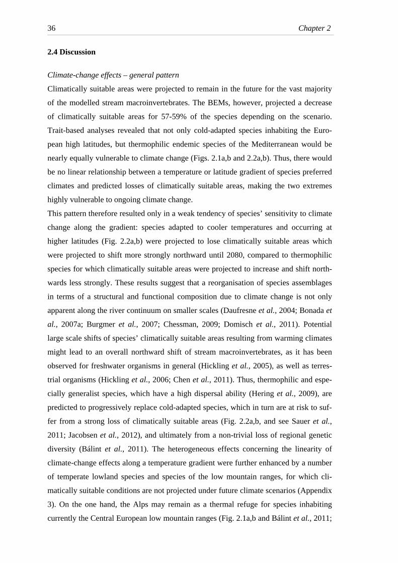
36 Chapter 2
2.4 Discussion
Climate-change effects – general pattern
Climatically suitable areas were projected to remain in the future for the vast majority
of the modelled stream macroinvertebrates. The BEMs, however, projected a decrease
of climatically suitable areas for 57-59% of the species depending on the scenario.
Trait-based analyses revealed that not only cold-adapted species inhabiting the Euro-
pean high latitudes, but thermophilic endemic species of the Mediterranean would be
nearly equally vulnerable to climate change (Figs. 2.1a,b and 2.2a,b). Thus, there would
be no linear relationship between a temperature or latitude gradient of species preferred
climates and predicted losses of climatically suitable areas, making the two extremes
highly vulnerable to ongoing climate change.
This pattern therefore resulted only in a weak tendency of species’ sensitivity to climate
change along the gradient: species adapted to cooler temperatures and occurring at
higher latitudes (Fig. 2.2a,b) were projected to lose climatically suitable areas which
were projected to shift more strongly northward until 2080, compared to thermophilic
species for which climatically suitable areas were projected to increase and shift north-
wards less strongly. These results suggest that a reorganisation of species assemblages
in terms of a structural and functional composition due to climate change is not only
apparent along the river continuum on smaller scales (Daufresne et al., 2004; Bonada et
al., 2007a; Burgmer et al., 2007; Chessman, 2009; Domisch et al., 2011). Potential
large scale shifts of species’ climatically suitable areas resulting from warming climates
might lead to an overall northward shift of stream macroinvertebrates, as it has been
observed for freshwater organisms in general (Hickling et al., 2005), as well as terres-
trial organisms (Hickling et al., 2006; Chen et al., 2011). Thus, thermophilic and espe-
cially generalist species, which have a high dispersal ability (Hering et al., 2009), are
predicted to progressively replace cold-adapted species, which in turn are at risk to suf-
fer from a strong loss of climatically suitable areas (Fig. 2.2a,b, and see Sauer et al.,
2011; Jacobsen et al., 2012), and ultimately from a non-trivial loss of regional genetic
diversity (Bálint et al., 2011). The heterogeneous effects concerning the linearity of
climate-change effects along a temperature gradient were further enhanced by a number
of temperate lowland species and species of the low mountain ranges, for which cli-
matically suitable conditions are not projected under future climate scenarios (Appendix
3). On the one hand, the Alps may remain as a thermal refuge for species inhabiting
currently the Central European low mountain ranges (Fig. 2.1a,b and Bálint et al., 2011;

Chapter 2
37
Sauer et al., 2011; Taubmann et al., 2011). On the other hand, lowland and downstream
species of the temperate region are expected to respond to warming temperatures in a
gain of suitable habitats (Mulholland et al., 1997; Daufresne et al., 2004; Domisch et
al., 2011), however species-specific ecological characteristics may play an important
role when predicting potential climate-change effects for these species (McPherson &
Jetz, 2007).
Complete losses of climatically suitable areas, as reported in our study for two species,
need to be approached carefully. As species records covered on average 81% of species’
known ranges, thus leaving space for a small amount of incomplete distributional data,
complete losses of climatically suitable areas are therefore likely to be overestimated
(Barbet-Massin et al., 2010; Sánchez-Fernández et al., 2011), nevertheless underlining
their high vulnerability to warming climates. Moreover, recent studies suggest that dis-
tributions of stream biota of running waters are not in climatic equilibrium and are still
likely to be influenced by post-glacial recolonization (Dehling et al. 2010; Hof et al.,
2012). Thus species, except Mediterranean / endemic ones, may not have reached all
potential habitats holding climatic suitability, influencing model calibration and thus
future projections.
Climate-change effects of trait-based species sets
Models confirmed our initial hypothesis regarding the higher losses of climatically suit-
able areas for endemic species than for non-endemics, while only differences in the
magnitude of latitudinal or longitudinal shifts of climatically suitable areas were pro-
jected for other trait-based sets. A majority of 85% of the endemic species occurring in
the Iberian-Macaronesian region were identified as climate-change losers under both
climate warming scenarios (Fig. 2.2a,b). The high endemicity in Southern Europe is a
result of the speciation during the Pleistocene (see e.g., Ribera & Vogler, 2004, and
references therein). Although dispersal was not limited in the BEMs, future climatically
suitable areas were found to remain only by a fraction within this region, indicating the
high vulnerability of these species to climate change (Bonada et al., 2009; Hering et al.,
2009; de Figueroa et al., 2010). Though stream macroinvertebrates of the Mediterra-
nean provide traits with a high resistance against droughts as well as a high resilience
after droughts (Bonada et al., 2007a), the question remains whether the magnitude of
warming temperatures and the declining amount of (summer) precipitation exceed be-
yond the adaptation ability of these species.

38 Chapter 2
Stronger northward shifts of both rare and generalist species’ climatically suitable areas
than for the respective counterparts, seem to be contradicting at the first glance. For rare
species, this implies that they would need to track temperature changes faster than
common species. Though species are capable of rapid range changes (Chen et al., 2011)
as well as plasticity in terms of adaptation to some degree (Hampe & Petit, 2005), po-
tential range changes depend strongly on species’ dispersal abilities and life history
characteristics. Limited habitat availability under warming climates (Heino et al., 2009)
will impose an additional major threat for stream macroinvertebrates. Predicted changes
in discharge patterns and droughts, combined with land use changes and large scale irri-
gation measures are predicted to contribute to increased habitat fragmentation, limiting
habitat availability beyond losses of climatically suitable areas in the future.
Amongst headwater, generalist and downstream river species, generalists are best buff-
ered against climate change impacts as shown by their ability to colonise northern Eu-
rope after the Pleistocene (see e.g., Hering et al., 2009, and references therein). They
tolerate a broad range of climatic conditions, enabling them to potentially take advan-
tage of suitable climates along a wider range of latitudes. In turn, the highest ratio of
climate-change loser species among the three groups was identified for headwater spe-
cies, which are restricted to cooler temperatures. For these species, shifts in climatically
suitable areas were not projected northwards as was the case for generalists, meaning
that they will lose climatically suitable areas within their ranges until 2080 because of a
the predicted summit trap, i.e., a decrease in available area with increasing altitudes.
However, as air temperatures may be a poor surrogate for depicting stream temperatures
in headwater reaches located in lower altitudes (sensu Caissie, 2006), potential changes
of climatically suitable areas were presumably underestimated, probably resulting in
even stronger losses of climatically suitable areas (Bálint et al., 2011; Sauer et al.,
2011). In turn, no strong geographic shifts were projected for downstream river species,
as they are predicted to gain climatically suitable areas due to climate warming (i.e.,
range filling, Table 2.2, Domisch et al., 2011), potentially influencing the downstream
community structure and composition (Daufresne et al., 2004).
The coarse resolution seemed to blur consistent patterns for specialists based on current
preference and life cycle. Streams and rivers across Europe are expected to respond
strongly to climate change due to increased temperatures and changes in annual as well
as seasonal precipitation patterns (Milly et al., 2005), resulting in discharge changes and
ultimately in current velocity. BEMs revealed a non-significant tendency of a high ratio
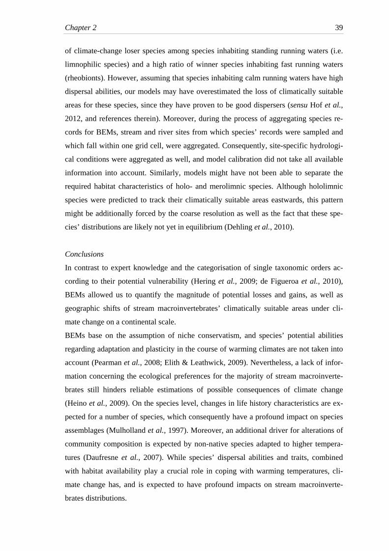
Chapter 2
39
of climate-change loser species among species inhabiting standing running waters (i.e.
limnophilic species) and a high ratio of winner species inhabiting fast running waters
(rheobionts). However, assuming that species inhabiting calm running waters have high
dispersal abilities, our models may have overestimated the loss of climatically suitable
areas for these species, since they have proven to be good dispersers (sensu Hof et al.,
2012, and references therein). Moreover, during the process of aggregating species re-
cords for BEMs, stream and river sites from which species’ records were sampled and
which fall within one grid cell, were aggregated. Consequently, site-specific hydrologi-
cal conditions were aggregated as well, and model calibration did not take all available
information into account. Similarly, models might have not been able to separate the
required habitat characteristics of holo- and merolimnic species. Although hololimnic
species were predicted to track their climatically suitable areas eastwards, this pattern
might be additionally forced by the coarse resolution as well as the fact that these spe-
cies’ distributions are likely not yet in equilibrium (Dehling et al., 2010).
Conclusions
In contrast to expert knowledge and the categorisation of single taxonomic orders ac-
cording to their potential vulnerability (Hering et al., 2009; de Figueroa et al., 2010),
BEMs allowed us to quantify the magnitude of potential losses and gains, as well as
geographic shifts of stream macroinvertebrates’ climatically suitable areas under cli-
mate change on a continental scale.
BEMs base on the assumption of niche conservatism, and species’ potential abilities
regarding adaptation and plasticity in the course of warming climates are not taken into
account (Pearman et al., 2008; Elith & Leathwick, 2009). Nevertheless, a lack of infor-
mation concerning the ecological preferences for the majority of stream macroinverte-
brates still hinders reliable estimations of possible consequences of climate change
(Heino et al., 2009). On the species level, changes in life history characteristics are ex-
pected for a number of species, which consequently have a profound impact on species
assemblages (Mulholland et al., 1997). Moreover, an additional driver for alterations of
community composition is expected by non-native species adapted to higher tempera-
tures (Daufresne et al., 2007). While species’ dispersal abilities and traits, combined
with habitat availability play a crucial role in coping with warming temperatures, cli-
mate change has, and is expected to have profound impacts on stream macroinverte-
brates distributions.

40 Chapter 3
Chapter 3
Choice of study area and predictors affect species distribution models
of stream macroinvertebrates
Abstract
Species distribution models (SDMs) are valuable and increasingly used tools for analy-
ses, such as conservation- or climate-change-related vulnerability analyses. However,
SDMs must be optimised for study area, predictors, and presence-absence data to avoid
false positive predictions. In stream ecosystems, for which such models were only re-
cently adopted, this optimisation is particularly challenging, as false positive predictions
may be projected in terrestrial areas and not in the stream network, with unknown ef-
fects on habitat suitability simulations. To test for effects derived from the use of differ-
ent study areas and predictors, we used consensus projections of a fixed set of 224
stream macroinvertebrate species, using five algorithms implemented in BIOMOD/R
(GLM, GAM, BRT, ANN, CTA). Four modelling designs were applied: (1) a continu-
ous study area without any discrimination between terrestrial and aquatic realms, (2)
results from this design masked a posteriori with a stream network, (3) the stream net-
work only considered as the study area during the model-building stage, and (4) same as
(3) but with a corrected set of predictors. The true skill statistic (TSS) and accuracy of
the consensus projections were not influenced by the different designs, as they were
consistently high (TSS: 0.80 to 1.00, accuracy: 0.70 to 0.96). The models built on a
stream network yielded a strong reduction in false positive predictions compared with
those built on a continuous area, whereas the differences derived from non-corrected vs.
corrected predictors were small. The models created in the stream network with cor-
rected predictors were able to diminish the false positive predictions by an average of
56%, yielding the highest rate among the four designs. SDMs of stream macroinverte-
brates should thus be built on a stream network rather than on a continuous area, and the
predictors should be chosen carefully. We discuss several methods for developing pre-
dictor accuracy to improve forecasts of potential climate-change effects on species’
ranges.
Sami Domisch, Mathias Kuemmerlen, Sonja C. Jähnig, Peter Haase. Submitted to
Freshwater Biology

Chapter 3 41
3.1 Introduction
Estimations of the potential effects of climate change on species’ ranges are important
for understanding species’ habitat suitability patterns under changing climatic condi-
tions and for mitigation and possible conservation efforts (Elith & Leathwick, 2009;
Araújo et al., 2011). Species distribution models (SDMs) are promising and increas-
ingly used tools for this task. One great challenge when using SDMs is their optimisa-
tion regarding study area, predictors, and presence-absence data to avoid false positive
predictions. In stream ecosystems, for which such models were only recently adopted,
this optimisation is particularly challenging, as false positive predictions may be pro-
jected in terrestrial areas and not in the stream network. The effects of building a model
on a continuous landscape as a study area, without taking into consideration the stream
network in which species were recorded (Cordellier & Pfenninger, 2008; Bálint et al.,
2011; Sauer et al., 2011), are unknown, which constitutes a major disadvantage for the
further development of models, e.g., in terms of sensitivity analyses. Landscape-based
models clearly provide a useful first approximation, e.g., in terms of climate-change-
related vulnerability analyses, such as the means by which warming and changes in pre-
cipitation patterns might affect species’ distributions (sensu Pearson & Dawson, 2003).
However, the distribution and abundance of freshwater biodiversity also depend on oth-
er factors too, considered in catchment-related variables (Poff, 1997). In the case of cer-
tain stream organisms, such as benthic macroinvertebrates or fish, stream flow condi-
tions are known to influence the composition of the community (Clausen & Biggs,
1997). Such variables are inevitably ignored in landscape-based models.
The choice of whether the continuous landscape or stream network is used as the study
area for predicting the distributions of stream macroinvertebrates has several relevant
aspects, but the issues of species’ presence-absence data and the choice of predictors
used for delineating species ranges are considered to be the most important. In general,
SDMs require both species’ presence and species’ absence data, which are combined
with environmental predictors that yield species’ habitat suitability after being extrapo-
lated in space or time. SDMs can be roughly divided into two groups depending on the
origin of the species records: presence-absence and presence-only SDMs (Elith &
Leathwick, 2009, and references therein). SDMs of the former type use species’ re-
corded absences and are thus based on species’ true environmental envelopes, whereas
those of the latter require background data or pseudo-absences for generating probabili-
ties of species’ habitat suitability. Because recorded absences of species are scarce,

42 Chapter 3
pseudo-absences are widely used (Lobo & Tognelli, 2011; Stokland et al., 2011). Obvi-
ously, the properties of pseudo-absences are highly dependent on the study area and can
be allocated either distant (i.e., on the continuous landscape) or near (within the stream
network) to species’ environmental envelopes, likely affecting model performance (Lo-
bo et al., 2010; Barbet-Massin et al., 2012). In general, Lobo et al. (2010) define three
types of species absences, which may be applied to stream ecosystems: contingent ab-
sences (i.e., the habitat is potentially suitable but the species is absent due to, e.g., peaks
in stream discharge changes or species’ lifecycles); environmental absences (e.g., lack
of favourable long-term temperature or physico-chemical conditions, Poff, 1997), and
methodological absences (e.g., sampling season and methodology, Haase et al., 2004;
Haase et al., 2006). The examples of contingent and methodological absences show that
true absence data of stream organisms are particularly difficult to record. Though the
use of pseudo-absences is partially seen as a violation of true ecological assumptions
and species’ niche occupancy, resulting ultimately in a reduction in the model accuracy,
this practise presents a suitable work-around solution for calibrating and fitting SDMs
in stream ecosystems (sensu Lobo et al., 2010). In the case of stream ecosystem model-
ling, the choice of study area is likely to affect the environmental absences, which can
be allocated either on the entire landscape or exclusively within the stream network.
Thus, the model accuracy and the quantity of species’ false positive predictions are like-
ly being affected because these absences differ in their distances to species’ recorded
presence records.
Second, the choice of the study area inevitably influences the choice of predictors used
in SDMs through the medium itself but also through scale, resolution, and availability
of the data. On a continuous landscape, coarse-scale predictors, such as air temperature
and precipitation, take priority over predictors describing stream-specific conditions
(e.g., stream type, flow accumulation), which play a larger role at fine scales (hierarchi-
cal modelling framework sensu Pearson & Dawson, 2003). In contrast, when moving
into finer scales, SDMs based on a stream network may include more specific predictors
that allow simple hydrological predictors, such as stream type, flow accumulation or
stream order, to be included, which are of relevance for characterising the habitat suit-
ability of stream assemblages and communities (Poff 1997). However, working at such
scales also means dealing with extra uncertainties. For instance, small-scale variations
of the stream topography are important to take into account, and predictors may need to
be corrected because of spatial differences between the underlying digital elevation

Chapter 3
43
model (DEM) and the digitised stream network layer. The correction of relevant predic-
tors based on the DEM can therefore have a significant effect on model performance
and thus on the projections of species’ habitat suitability (Adriaenssens et al., 2004).
In this study, we analyse the effects of the extent of the modelled area and the choice of
predictors on species’ predictions using stream macroinvertebrates, a very important
organism group in streams used as indicator species for assessing stream condition.
Based on a fixed set of species, we vary the choice of study area from the continuous
landscape to a stream network during and after the model-building stage using a fixed
set of predictors. Moreover, we vary the choice of predictors from a non-corrected to a
corrected set within a fixed study area. We hypothesise that (1) the usage of a continu-
ous landscape as the study area yields a high degree of species’ false positive predic-
tions because the terrestrial and aquatic realms are confounded at the model-building
stage, (2) using a stream network as the study area at the model-building stage will in-
crease the model accuracy and strongly reduce the number of false positive predictions
because pseudo-absences will not include those ranging beyond species environmental
absences, i.e., the terrestrial areas, and (3) a corrected set of predictors during the mod-
el-building stage will further enhance the model accuracy and reduce the number of
false positive predictions, as it may delineate species’ environmental envelopes, and
thus the environmental absences, more accurately than a non-corrected set.
3.2 Methods
Modelling designs
Four different modelling designs were applied (see Fig. 3.1a-d). In the most basic ap-
proach, we modelled species’ distributions on a continuous landscape area (hereafter
referred to as a ‘landscape’ design, Fig. 3.1b), without any discrimination between
streams and the terrestrial area.
In the second design, a stream network mask was applied to the ‘landscape’ projections,
as the species are supposed to inhabit the streams and rivers (hereafter ‘landscape
masked’, Fig. 3.1c). This design is thus identical to the previous ‘landscape’ design ex-
cept that it is restricted to the grid cells of the river network.
In the third design, the stream network area was masked prior to fitting the models;
thus, only the stream network was considered at the model-building stage (Fig. 3.1d).
For this design, we used an identical set of predictors as in the ‘landscape’ and ‘land-
scape masked’ designs (hereafter referred to as the ‘stream network’ design).

44 Chapter 3
The last design also modelled species’ distributions on the stream network, but used a
partially different set of predictors to test for effects derived from using corrected pre-
dictors (hereafter referred to as the ‘stream network corrected’ design, Fig. 3.1d).
Figure 3.1 (a) Scheme of a stream section (black lines); the grid cells represent the division of the area for modelling. (b-d) Four modelling designs based on the stream section: (b) ‘land-scape’, (c) ‘landscape masked’, (d) ‘stream network’, and ‘stream network corrected’ design, the latter of which used a different set of predictors. The numbers represent presence records (1) and pseudo-absences (0), respectively. The grey cells in the ‘landscape masked’ design repre-sent the terrestrial realm and was masked after the model-building stage.
Area for model calibration
Our models were calibrated either on the continuous area of Germany (5°86´–15°04´E,
47°27´–55°06´N, Fig. 3.2a,b) or on the stream network within this area (LAWA, 2003).
The area ranged from the foothills of the Alps to the coast of the North and Baltic Seas.
The running waters of the stream network included all river sizes from small alpine
streams (catchment size 10–100 km2) to large lowland rivers (catchment size > 10,000
km2). The resolution for both areas was 0.01 degree (ca. 1 km2), and the spatial extents
were 321,735 and 136,207 grid cells for the continuous area and stream network, re-
spectively.
All of the models were fitted using these extents to overcome the limitation of using
truncated environmental gradients for calibrating models within species’ known ranges
(Thuiller et al., 2004). For the final assessment of model results, we considered an area
limited to four federal states (Westphalia, Hesse, Thuringia, Baden-Wuerttemberg), as
this area provides the highest density of species records, i.e., a high accuracy of species
presence data (Fig. 3.2b, shaded area, hereafter referred to as the ‘study area’).
1 0 10
00 1
00
1 0 10
00 1
00
1 0 10
00 1
00
1 0 10
00 1
00
0 1 1
01
0
0 1 1
01
0
(a) (b) (c) (d)

Chapter 3
45
15°0'0"E12°0'0"E9°0'0"E6°0'0"E
54°0'0"N
51°0'0"N
48°0'0"N±0 10050
km
(a) (b)
Figure 3.2 (a) The location of the study area in Central Europe. (b) The stream network of Germany (grey lines) and all presence records (points) used for calibrating the models. The shaded area represents the study area used for the final assessment.
Species data
Species records were obtained from three national databases (Umweltbundesamt; Hessi-
sches Landesamt für Umwelt und Geologie; and Landesamt für Umwelt, Messungen
und Naturschutz Baden-Württemberg, unpublished data). These databases provide
stream macroinvertebrate data from surveys conducted in spring from 2002 to 2008 and
hold a total of 55,513 species presence records from 2,849 sites within the entire area
used for calibrating the models. As a precondition for selection in our study, species
needed to have at least 10 presence records listed within the study area (Stockwell &
Peterson, 2002). Individual models were fitted for the 269 species that fulfilled this cri-
terion.
Environmental predictors
For each modelling design, we used 10 environmental predictors consisting of climatic,
land cover and stream-specific predictors (Table 3.1). Only the predictors relevant for
describing the distributions of stream macroinvertebrates were selected, and pairwise
correlations were used to reduce the initial candidate set of 35 predictors (-0.7 < r < 0.7,
Green, 1979).
The present climate data were generated by averaging interpolated mean monthly cli-
mate data from a 30-year time period (1980-2010) at a resolution of 0.01 degree, ob-
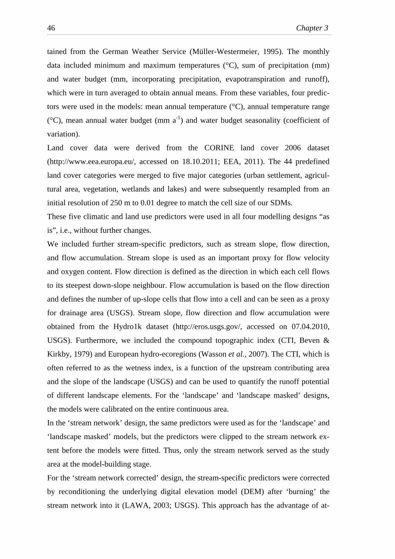
46 Chapter 3
tained from the German Weather Service (Müller-Westermeier, 1995). The monthly
data included minimum and maximum temperatures (°C), sum of precipitation (mm)
and water budget (mm, incorporating precipitation, evapotranspiration and runoff),
which were in turn averaged to obtain annual means. From these variables, four predic-
tors were used in the models: mean annual temperature (°C), annual temperature range
(°C), mean annual water budget (mm a-1) and water budget seasonality (coefficient of
variation).
Land cover data were derived from the CORINE land cover 2006 dataset
(http://www.eea.europa.eu/, accessed on 18.10.2011; EEA, 2011). The 44 predefined
land cover categories were merged to five major categories (urban settlement, agricul-
tural area, vegetation, wetlands and lakes) and were subsequently resampled from an
initial resolution of 250 m to 0.01 degree to match the cell size of our SDMs.
These five climatic and land use predictors were used in all four modelling designs “as
is”, i.e., without further changes.
We included further stream-specific predictors, such as stream slope, flow direction,
and flow accumulation. Stream slope is used as an important proxy for flow velocity
and oxygen content. Flow direction is defined as the direction in which each cell flows
to its steepest down-slope neighbour. Flow accumulation is based on the flow direction
and defines the number of up-slope cells that flow into a cell and can be seen as a proxy
for drainage area (USGS). Stream slope, flow direction and flow accumulation were
obtained from the Hydro1k dataset (http://eros.usgs.gov/, accessed on 07.04.2010,
USGS). Furthermore, we included the compound topographic index (CTI, Beven &
Kirkby, 1979) and European hydro-ecoregions (Wasson et al., 2007). The CTI, which is
often referred to as the wetness index, is a function of the upstream contributing area
and the slope of the landscape (USGS) and can be used to quantify the runoff potential
of different landscape elements. For the ‘landscape’ and ‘landscape masked’ designs,
the models were calibrated on the entire continuous area.
In the ‘stream network’ design, the same predictors were used as for the ‘landscape’ and
‘landscape masked’ models, but the predictors were clipped to the stream network ex-
tent before the models were fitted. Thus, only the stream network served as the study
area at the model-building stage.
For the ‘stream network corrected’ design, the stream-specific predictors were corrected
by reconditioning the underlying digital elevation model (DEM) after ‘burning’ the
stream network into it (LAWA, 2003; USGS). This approach has the advantage of at-

Chapter 3
47
taching the information concerning the sources and mouths of streams to the DEM. We
then used ArcHydro tools (Maidment, 2005) to fill sinks (i.e., artificial valleys in the
DEM derived from inaccurate remote sensing data, disconnecting continuous streams)
and recalculated the stream slope, flow direction and flow accumulation more accu-
rately. Stream order (Strahler, 1957) was included in the models as a proxy for stream
size and distance to source. Furthermore, stream type was included as a proxy for
catchment area, ecoregion and geology (for a detailed description of German stream
types, see http://www.fliessgewaesser-bewertung.de/en/, Pottgiesser & Sommerhäuser,
2004). The stream order and stream type were derived from LAWA (2003).
Table 3.1 The predictors used for calibrating SDMs for the four modelling designs.
Predictors Landscape Landscape
masked Stream network
Stream net-work corrected
Mean annual temperature x x x x Annual temperature range x x x x Mean annual water budget x x x x Water budget seasonality x x x x Land cover x x x x Stream slope x x x Stream slope corrected x Flow direction x x x Flow direction corrected x Flow accumulation x x x Flow accumulation corrected x Compound Topographic Index x x x Stream order x Hydro-Ecoregions x x x Stream type x
Species distribution modelling
SDMs were generated using five algorithms as implemented in the R package BIO-
MOD (generalised linear models, GLM; generalised additive models, GAM; boosted
regression trees, BRT; artificial neural networks, ANN; and classification tree analysis,
CTA; Thuiller et al., 2009; R Development Core Team, 2011). Single models were cal-
ibrated by splitting species occurrence data randomly into a training set (70%) and a
testing set (30%, Araújo et al., 2005). Absence records were not available, so we used
pseudo-absences, which were allocated throughout the entire landscape or along the
stream network, depending on the modelling design. Each design used 10,000 randomly

48 Chapter 3
drawn pseudo-absences, referring to Stokland et al., (2011) and Barbet-Massin et al.,
(2012), who showed that excluding pseudo-absence data involves arbitrary assumptions
about unsuitable environments for the species being modelled, and Lobo & Tognelli
(2011), who recommend the incorporation of many pseudo-absences to obtain more
accurate predictive models.
Each algorithm used a tenfold cross validation that yielded an average model for each
species and algorithm, and the prevalence was kept constant at 0.5 for all species
(weighted prevalence, Barbet-Massin et al., 2012). The average models, comprised of
the single models, were calibrated on 100% of the species data, as the exclusion of pres-
ence records significantly increases the amount of uncertainty (Araújo et al., 2009).
These average models were then projected to the whole study area (i.e., the entire terri-
tory or stream network, Fig. 3.2b). Model evaluation was conducted by means of the
true skill statistic (TSS), which has been shown to be superior in measuring the per-
formance of SDMs when the predictions are expressed in presence-absence maps that
enable effective model comparisons (Allouche et al., 2006). TSS scores incorporate
sensitivity (true positive predictions) and specificity (true negative predictions) and
range from 0 to 1, of which 0 describes a model no better than random, and 1 describes
a perfect agreement with the observed data. The uncertainty derived from different algo-
rithms was reduced using a consensus projection for each species with weighted aver-
ages (WA) based on the TSS scores of single model outputs for each species and algo-
rithm (Marmion et al., 2009). The relative importance of each algorithm for the final
consensus models was obtained by multiplying the averaged TSS score with a weight
decay of 1.6 (default settings). To overcome the limitation of mixing weak models with
robust ones, we set a threshold of TSS > 0.4 for models to be included in the consensus,
adopting methods from (Engler et al., 2011). At least two models were required to re-
ceive a TSS score higher than 0.4; otherwise, no consensus projection was created, and
the species was removed from further analyses. Occurrence probability maps of present
projections were finally transformed into binary presence-absence maps by applying a
cut-off value that minimises the difference between sensitivity and specificity, based on
the TSS scores (Jimenez-Valverde & Lobo, 2007). This modelling procedure was per-
formed for each species and design, resulting in a total of 45,192 models.

Chapter 3
49
Comparison of modelling designs
To keep the study design balanced, results were only analysed for those species for
which consensus projections were created for all designs. The relative predictor contri-
butions show how each predictor contributes to each species’ distributions. The results
of the algorithms were averaged using the same weighting factor that was used for
building the consensus projections and were finally averaged over all of the species for
each modelling design. The TSS scores of species’ consensus projections were evalu-
ated among all modelling designs. In this comparison, the relative predictor contribu-
tions and the TSS scores rely on the entire area for calibrating the SDMs.
For all further analyses, the consensus projections were masked to the extent of the
study area (94,661 and 41,590 grid cells available for landscape and stream network,
respectively).
Because we were interested in the model performance in our study area, we assessed the
model validity, i.e., the accuracy and significance of the consensus projections within
this area. Adopting methods from Anderson et al. (2003), the accuracy was calculated
by means of exact one-tailed binomial probabilities of presence records falling into grid
cells classified as suitable. The model accuracy ranged from 0, for a consensus projec-
tion no better than random, to 1, for the maximum success rate. For a more detailed de-
scription of this method, see Anderson et al. (2003). To measure the significance of the
models, we tested whether the probability of making n successful predictions is higher
than by chance alone (where n is the number of presence records).
To evaluate the size of the area predicted to be suitable habitat for each species and
modelling design, we compared the sum of the grid cells classified as suitable among
the different designs derived from binary consensus projections relative to the available
study area (relative occurrence area ROA, Lobo et al., 2008). Furthermore, we calcu-
lated pairwise differences in the number of grid cells classified as suitable between the
different modelling designs by means of paired t-tests.
To explore the effect of how and where the suitable habitat area differed among the
modelling designs, the proportion of overlapping grid cells classified as suitable was
compared. These proportions were evaluated by overlaying single species’ projections
from the different designs and identifying the number of overlapping grid cells classi-
fied as suitable.
The results of the TSS scores, model accuracy and ROA were analysed using a one-way
ANOVA to evaluate the differences between the different designs. Percent data were

50 Chapter 3
arcsin-transformed prior to the analyses, and where appropriate, data were log-
transformed to meet the assumptions of normality and homogeneity of variances. Addi-
tionally, a Kruskal-Wallis-ANOVA was computed for data with heterogeneous vari-
ances after transformation. Post-hoc tests (Tukey HSD) were performed to detect sig-
nificant differences between model results.
3.3 Results
For the ‘landscape’, ‘landscape masked’, ‘stream network’ and ‘stream network cor-
rected’ designs, consensus projections were created for 251 (93%), 251 (93%), 232
(86%) and 237 (88%) species out of the initial set of 269 species, respectively. From
these, 224 species from 17 macroinvertebrate orders were successfully modelled in all
of the designs and were thus considered for further analyses (Appendix 4). For all of the
modelling designs, the predictors that contributed most to the consensus projections
were hydro-ecoregions and stream type, as well as the mean annual temperature and
annual temperature range (Fig. 3.3). The consensus TSS scores for all of the designs and
species were consistently high, ranging from 0.80 to 1.00, and did not differ signifi-
cantly between modelling designs (Kruskal-Wallis ANOVA: H3 = 7.48, P = 0.058).
Mean (±SD) relative contribution (%)
0 10 20 30 40 50 60
Stream typeHydro-Ecoregions
Stream orderCompound Topographic Index
Flow accumulationFlow direction
Stream slopeLand cover
Water budget seasonalityMean annual water budgetAnnual temperature rangeMean annual temperature
Stream network correctedStream networkLandscape / Landscape masked
Figure 3.3 The relative predictor contributions of the final consensus models for the four mod-elling designs, averaged over all species.
The results of model accuracy, i.e., the rate of successful predictions of known occur-
rence locations, revealed no significant differences between the modelling designs
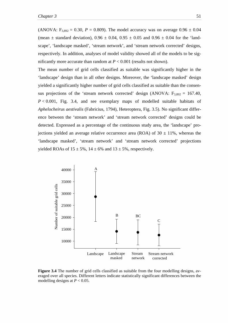
Chapter 3
51
(ANOVA: F3,892 = 0.30, P = 0.809). The model accuracy was on average 0.96 ± 0.04
(mean ± standard deviation), 0.96 ± 0.04, 0.95 ± 0.05 and 0.96 ± 0.04 for the ‘land-
scape’, ‘landscape masked’, ‘stream network’, and ‘stream network corrected’ designs,
respectively. In addition, analyses of model validity showed all of the models to be sig-
nificantly more accurate than random at P < 0.001 (results not shown).
The mean number of grid cells classified as suitable was significantly higher in the
‘landscape’ design than in all other designs. Moreover, the ‘landscape masked’ design
yielded a significantly higher number of grid cells classified as suitable than the consen-
sus projections of the ‘stream network corrected’ design (ANOVA: F3,892 = 167.40,
P < 0.001, Fig. 3.4, and see exemplary maps of modelled suitable habitats of
Aphelocheirus aestivalis (Fabricius, 1794), Heteroptera, Fig. 3.5). No significant differ-
ence between the ‘stream network’ and ‘stream network corrected’ designs could be
detected. Expressed as a percentage of the continuous study area, the ‘landscape’ pro-
jections yielded an average relative occurrence area (ROA) of 30 ± 11%, whereas the
‘landscape masked’, ‘stream network’ and ‘stream network corrected’ projections
yielded ROAs of 15 ± 5%, 14 ± 6% and 13 ± 5%, respectively.
Num
ber o
f sui
tabl
e gr
id c
ells
10000
15000
20000
25000
30000
35000
40000
B BCC
A
Landscape masked
Stream network
Stream network corrected
Landscape
Figure 3.4 The number of grid cells classified as suitable from the four modelling designs, av-eraged over all species. Different letters indicate statistically significant differences between the modelling designs at P < 0.05.

52 Chapter 3
Figure 3.5 (a) Stream network in the study area with a frame delineating the cut-out for figures b-e. (b-e) Modelled suitable habitats for Aphelocheirus aestivalis (Fabricius, 1794), Heteroptera, derived from the different modelling designs: (b) ‘landscape’, (c) ‘landscape masked’, (d) ‘stream network’, and (e) ‘stream network corrected’ design. The shaded area represents mod-elled suitable habitat, and the circles mark presence records. The evaluations of pairwise differences based on the number of grid cells classified as
suitable differed significantly between all combinations of the different designs (Paired
t-tests, Table 3.2).
The percentage of overlapping grid cells classified as suitable between the modelling
designs was highest between the ‘landscape masked’ and ‘stream network’ designs (93
± 7%) and lowest between the ‘landscape’ and ‘stream network corrected’ designs (36 ±
6%, Appendix 5).
Table 3.2 Pairwise differences of grid cells classified as suitable between modelling designs, expressed as the mean number and percentage (± standard deviations) with t-statistics.
Landscape Landscape masked Stream network 14623 ± 5758
(51 ± 20%) Landscape masked
t223=38.01, P <0.001 15024 ± 6097 401 ± 1778
(52 ± 21%) (3 ± 13%) Stream network t223=36.88, P <0.001 t223=3.38, P <0.001
16158 ± 6931 1535 ± 2782 1134 ± 2782 (56 ± 24%) (11 ± 19%) (8 ± 20%) Stream network
corrected t223=34.89, P <0.001 t223=8.73, P <0.001 t223=6.10, P <0.001
Ü 0 10050 km
B
A
C D E(c) (d) (e)
(a)
(b)
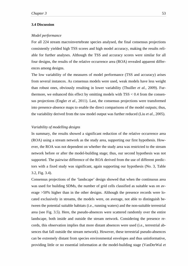
Chapter 3
53
3.4 Discussion
Model performance
For all 224 stream macroinvertebrate species analysed, the final consensus projections
consistently yielded high TSS scores and high model accuracy, making the results reli-
able for further analyses. Although the TSS and accuracy scores were similar for all
four designs, the results of the relative occurrence area (ROA) revealed apparent differ-
ences among designs.
The low variability of the measures of model performance (TSS and accuracy) arises
from several instances. As consensus models were used, weak models have less weight
than robust ones, obviously resulting in lower variability (Thuiller et al., 2009). Fur-
thermore, we enhanced this effect by omitting models with TSS < 0.4 from the consen-
sus projections (Engler et al., 2011). Last, the consensus projections were transformed
into presence-absence maps to enable the direct comparisons of the model outputs; thus,
the variability derived from the raw model output was further reduced (Liu et al., 2005).
Variability of modelling designs
In summary, the results showed a significant reduction of the relative occurrence area
(ROA) using a stream network as the study area, supporting our first hypothesis. How-
ever, the ROA was not dependent on whether the study area was restricted to the stream
network before or after the model-building stage; thus, our second hypothesis was not
supported. The pairwise difference of the ROA derived from the use of different predic-
tors with a fixed study was significant, again supporting our hypothesis (No. 3, Table
3.2, Fig. 3.4).
Consensus projections of the ‘landscape’ design showed that when the continuous area
was used for building SDMs, the number of grid cells classified as suitable was on av-
erage >50% higher than in the other designs. Although the presence records were lo-
cated exclusively in streams, the models were, on average, not able to distinguish be-
tween the potential suitable habitats (i.e., running waters) and the non-suitable terrestrial
area (see Fig. 3.5). Here, the pseudo-absences were scattered randomly over the entire
landscape, both inside and outside the stream network. Considering the presence re-
cords, this observation implies that more distant absences were used (i.e., terrestrial ab-
sences that fall outside the stream network). However, these terrestrial pseudo-absences
can be extremely distant from species environmental envelopes and thus uninformative,
providing little or no essential information at the model-building stage (VanDerWal et

54 Chapter 3
al., 2009; Lobo et al., 2010). Ultimately, pseudo-absences within and outside the stream
network were treated equally, classifying grid cells of both the aquatic and terrestrial
realms as non-suitable for the species. Consequently, there was no differentiation of the
truly non-suitable (terrestrial) and environmental (aquatic) absences in the models, lead-
ing to higher false positive predictions than were observed in the other three designs.
An exception in the exclusion of terrestrial absences would be merolimnic species
(aquatic larval stage and terrestrial adult stage), where the transition between absences
falling inside and outside the stream network is smooth. Because the terrestrial area be-
longs to the range of the species, the omission of this area would lead to a truncation of
these species’ environmental envelopes. However, presence records need to be available
for both life stages, as the different life stages clearly have contrasting habitat prefer-
ences, and they need to be treated as two different modelling subjects (Domisch et al.,
2011).
The ‘landscape masked’ design, i.e., applying a stream network mask on the ‘landscape’
projections afterwards, was effective in eliminating an average of 51% of the false posi-
tive predictions that fell outside the stream network (Table 3.2). Although it is possible
to further reduce these errors, as shown by the designs relying on the stream network in
the model-building stage, this design is, nevertheless, useful in reducing the a priori
truly non-suitable (i.e., terrestrial) habitats.
In contrast, the ‘stream network’ design used only absences within the stream network,
i.e., their potentially suitable habitat. Surprisingly, no clear advantage was yielded from
this design concerning the reduction of false positive predictions. The differences rela-
tive to the ‘landscape masked’ design appear to be negligible, as shown by the small
difference between the grid cells classified as suitable (on average, 3%, Table 3.2) to-
gether with the high degree of overlapping grid cells classified as suitable (on average,
93%, Appendix 5); hence, the choice of masking the study area to the stream network
before or after calibrating the models appears to be negligible when using random pseu-
do-absences. These results suggest that the information contained in the predictors used
in this study for the ‘landscape masked’ and ‘stream network’ designs is as accurate as
possible, regardless of the modelling extent. Thus, the fact that a model is fitted with the
spatial extent of a stream network does not improve the predictions per se. It is the fact
that the extent of the model projection (i.e., the result) is restricted to the ‘stream net-
work’ that improves the model outcome by limiting the false positive predictions.

Chapter 3
55
The question remains of how types of species’ (pseudo-) absence records perform in a
stream network. Though, e.g., Stokland et al. (2011) and Barbet-Massin et al. (2012)
recommend using random pseudo-absences, non-random distributions, e.g., convex or
alpha hulls (Burgman & Fox, 2003) and species’ range envelope models (SRE, Thuiller
et al., 2009) could also provide suitable methods for creating species’ pseudo-absences.
As species’ true absence records are difficult to obtain, the interconnectedness of
streams may allow the assumption that species occupy the stream reaches between the
most upper and most lower presence records in the stream network via convex or alpha
hulls, classifying the reaches beyond as potential areas for drawing pseudo-absences via
SREs.
The lowest rate of false positive predictions was derived from the ‘stream network cor-
rected’ design. In this design, the number of grid cells classified as suitable was lowest
compared with the other designs (on average, a difference of 56%, Table 3.2, Figs 3.4
and 3.5); however, the model accuracy was not affected, being consistently high (Ap-
pendix 4). The choice of corrected variables thus has the potential to further diminish
the degree of false positive predictions, as the number of grid cells classified as suitable
differed on average by 8% compared with the ‘stream network’ design. The results from
this design rely very strongly on the additional predictors that, in our case, are intended
to incorporate the hydrologic qualities of the catchment. The predictor stream type adds
to the model information about the catchment characteristics, such as the catchment
size, ecoregion and geology. This variable turned out to be highly relevant at this reso-
lution (0.01 degree), and it displaced other variables from the importance ranking and
even reduced the importance of further corrected hydrologic variables employed in this
modelling procedure.
Whither from here?
Species distribution models for stream macroinvertebrates are still in the early stages of
development. We recommend that, as first steps, a stream network should have prefer-
ence over a continuous area as study area to reduce false positive predictions, as model
accuracy appears not to be diminished by this option. Furthermore, a non-corrected set
of predictors should not be used “as is”, but predictors should be carefully selected or
corrected to delineate species’ specific environmental envelopes for predicting their
distributions.
56 Chapter 3
Although the first proposal can easily be applied on the appropriate scale and resolution,
the latter proposal is a major obstacle because of the scarcity of data ready for model-
ling. Thus, the development of suitable interpolation techniques should be envisaged, as
data in streams are mostly unavailable in a (stream-) continuous but in a point-wise pat-
tern. Thus, these point data, e.g., the sampling points of physico-chemical measure-
ments, must be transformed into continuous predictors along stream sections. Simple
interpolations are not sufficient for this task, as confluences of streams of different or-
ders interfere with direct interpolations. Thus, there is an urgent need to develop the
underlying methodology for taking into account single-point data that hold relevant in-
formation describing the environmental conditions of streams.
Moreover, SDMs on a stream network currently rely on the information for single grid
cells without taking into account the impact of adjacent cells. Though this approach is a
gross simplification of the stream environments, it is a useful first approximation for
predicting species’ vulnerabilities to climate warming (e.g., Domisch et al. 2011; Sauer
et al., 2011). However, future modelling studies should rely instead on the upstream
contributing areas influencing the grid cells located below by joining the information of,
e.g., precipitation or land use within single subcatchments and evaluating their effects
on the grid cells located below. Similarly, a buffer of riparian land use should be in-
cluded via the adjacent grid cells located along the stream network, having an effect on
the streams in the immediate vicinity. Combined, these approaches should clearly en-
hance the accuracy of predictors used in SDMs.
Ultimately, these improved methods for SDMs for stream macroinvertebrates could be
used to evaluate the climate change-related vulnerability of species more accurately
than is now possible, not only to understand the possible effects of single predictors at
the species level but also to gain knowledge about potential climate-change impacts on
species assemblages and to put forward suitable mitigation strategies at the catchment
scale. In this way, more accurate predictions of possible species ranges and their chang-
es in different future climate scenarios can help to delineate detailed and more cost-
effective conservation efforts to be undertaken.

Summary and general conclusions 57
Summary and general conclusions
Climate change is predicted to have severe impacts on species’ distributions, especially
for those inhabiting stream ecosystems due to warming temperatures and changes in
precipitation patterns, resulting in a increased frequency of floods and droughts (Sala et
al., 2000; Xenopoulos et al., 2005; Döll & Zhang, 2010). To understand to which extent
benthic stream macroinvertebrates are impacted by climate change, there is a need to
gain further insights into species’ potential susceptibility to climate warming. In this
context, species distribution models (SDMs) offer a useful tool to forecast the potential
impact of climate warming on species habitat suitability by relating species presences
and absences with environmental predictors at the locations of those (Elith & Leath-
wick, 2009).
The main objective of this thesis was to investigate potential patterns of stream macro-
invertebrates’ distributions under future climate change scenarios of the Intergovern-
mental Panel on Climate Change (IPCC, 2007) by means of SDMs. Specifically, the
purpose was to explore if and how species’ habitat suitability would be affected under
warming climates on different spatial scales, i.e. in the lower mountain ranges of Ger-
many (Chapter 1), and across Europe (Chapter 2). Further, the emphasis lied on investi-
gating how model projections depend on the study area and the predictors used by ap-
plying four modelling designs for a fixed set of species within Germany (Chapter 3).
In summary, projections of future potential suitable habitats for species along the river
continuum within the lower mountain ranges of Germany allowed to identify possible
climate-change winner and loser species depending on their overall gain or loss of suit-
able habitat until the year 2080 (Fig. 1.5c,d). Next to an uphill shift of species’ suitable
habitats along the river continuum, modelled changes of species’ habitat suitability
showed a clear relationship between the mean temperature of occurrence, i.e. the ther-
mal preference, and future habitat suitability, therefore supporting the first hypothesis
(H1, see General Introduction). Specifically, cold-adapted headwater species occurring
at higher altitudes were projected to lose suitable habitat, while gains were projected for
warm-adapted river species occurring in downstream reaches. This dependency of spe-
cies’ thermal preferences on potential climate-change effects could also be observed on
a continental scale for a large number of species (Fig. 2.2a,b): here, cold-adapted and
high-latitude species were projected to lose climatically suitable areas, whereas those of

58 Summary and general conclusions
warm-adapted and low-latitude species were projected to expand. This pattern was
however weakened due to a large number of endemic species of the Iberian-
Macaronesian region that were projected as potential climate-change losers by the year
2080. The second hypothesis (H2) was therefore supported by model projections.
Whereas modelling results on a smaller scale revealed that species would track their
climatically suitable areas uphill (Fig. 1.4), model projections on a large scale indicated
that an overall shift into a north-easterly direction of habitat suitability would occur in
Europe (Fig. 2.1a,b). These results corroborate long-term studies, in which these overall
patterns have been observed over the last decades for freshwater as well as terrestrial
organisms (e.g., Hickling et al., 2005; Chen et al., 2011). Model projections underpin
especially the high susceptibility of cold-adapted stream macroinvertebrates to warming
climates (Daufresne et al., 2007; Chessman, 2009). These species would likely encoun-
ter a summit trap and therefore a ‘nowhere to go situation’ as a consequence of the loss
of climatically suitable areas (Sala et al., 2000; Bálint et al., 2011; Sauer et al., 2011).
Here, it is important to consider that possible impacts of warming climates may reach
far beyond projected changes in habitat suitability. Since these cold-adapted species
occur as highly isolated populations in mountainous ecosystems, contractions of habitat
suitability could result in a reduction of population size or even population extinctions,
possibly leading to a loss in genetic diversity (Bálint et al., 2011; Taubmann et al.,
2011). Likewise, for downstream reaches of the river continuum, projected range ex-
pansions for warm-adapted river species would likely result in changes in community
structure and species composition (Mulholland et al., 1997). In addition, warming tem-
peratures have shown to facilitate the establishment of non-indigenous species (Dau-
fresne et al., 2008), further enhancing changes in species assemblages depending on
their potential characteristics as, for instance, keystone or ecosystem engineering spe-
cies (Dudgeon et al., 2006; Strayer, 2010).
Projected overall losses and gains of generalist species’ habitat suitability (i.e., species
occurring over a wide range along the river continuum) did not reach the magnitude of
those projected for cold-adapted or warm-adapted species, neither on a small (Fig.
1.5a,b) nor on a larger spatial scale (Fig. 2.2a,b). Models thus propose these species to
be best buffered against impacts of climate-change scenarios among the three species
groups. These species tolerate wide thermal ranges, a fact that is also shown by their
large geographical ranges due to their ability to colonise northern Europe after the Pleis-
tocene during cyclic glaciations and ice retreats (Bonada et al., 2009; Hering et al.,

Summary and general conclusions
59
2009). In contrast, these geological events resulted in a high endemicity in the Mediter-
ranean region due to speciation (e,g., Bonada et al., 2009, and references therein). These
endemic species have unique habitat requirements, and model projections revealed that
endemics of the Iberian Peninsula would be at high risk to warming climates due to a
loss of climatically suitable areas (Figs 2.1a,b and 2.2a,b), corroborating their high vul-
nerability to warming climates. Ultimately, climate change is likely to pose a major
threat to this biodiversity hotspot (Malcolm et al., 2006).
In addition to the similar patterns regarding the thermal sensitivity to climate warming
for the two studies, suitable habitats were projected to remain for most of the modelled
species in the lower mountain ranges and Europe, respectively (Chapter 1 and 2). These
results underline the consistency of climate-change effects derived from SDM projec-
tions on different spatial scales. However, model projections regarding the exact magni-
tude of geographical shifts, losses and gains of habitat suitability may not be compared
directly between these two approaches to infer possible species-specific alterations in
habitat suitability. Instead, these comparisons are useful to detect the overall pattern and
the direction of possible changes in species distributions (Araújo et al., 2005). For in-
stance, only coarse-scale bioclimatic predictors sensu Whittaker et al. (2007) were used
on the continental scale (Chapter 2), which did not account for specific hydrologic re-
gimes in streams and rivers. Similarly, the methodological study (Chapter 3) showed
that model projections for stream macroinvertebrates depend greatly on the study area
and on the predictors used. The SDMs built in a stream network and with corrected pre-
dictors were able to reduce commission errors, i.e., false positive predictions on average
by 56% compared to projections generated on a continuous area and non-corrected pre-
dictors, therefore reducing a considerable amount of uncertainties in model projections.
Though the third hypothesis was therefore supported (H3), model statistics were how-
ever not affected by different modelling designs by means of the true skill statistic
(TSS, incorporating true positive and negative predictions, Allouche et al., 2006) or
model validity, i.e., the accuracy and significance of the projections (Anderson et al.,
2003). This has important implications for modelling stream macroinvertebrates’ distri-
butions, as solely relying on model statistics would not be sufficient. Instead, the design
using a stream network during model calibration together with corrected predictors
should be preferred over an area-based approach and non-corrected predictors. The ad-
vantage of a stream network is, however, dependent on the spatial scale, and is of minor
relevance for a large-scale study such as for Europe (Chapter 2, grid cells were ap-

60 Summary and general conclusions
proximately 10 km2). Nevertheless, the direction of projected climate-change induced
shifts in habitat suitability of the two modelling approaches (Chapter 1 and 2) remain
similar, and support the observed vulnerability of stream macroinvertebrates to warming
climates.
The studies in this thesis focus essentially on possible changes of future habitat suitabil-
ity under climate change scenarios, assuming species’ thermal preferences to remain
constant over time, and without taking biotic interactions or species-specific migration
and dispersal abilities into account. The assumption of niche conservatism, and whether
it could or should be avoided in habitat suitability models in general, is a key question
since the early use of these correlative models (e.g., Pearman et al., 2008). Neverthe-
less, forecasts of species distributions derived from SDMs should thus be seen as a first
assessment of climate-change related vulnerability analyses of species, giving insights
into possible patterns derived from warming climates. For instance, SDMs have been
successfully applied on various fields related to climate change, ranging from conserva-
tion planning and identification of suitable habitat for rare species, to study possible
migration routes of invasive species (reviewed in Elith & Leathwick, 2009 and Araújo
& Peterson, 2012).
Next to the direction of climate-change effects (i.e., losses or gains of suitable habitats),
SDMs provide the information where these changes would likely occur. Concerning the
modelled altitudinal and / or latitudinal shifts of future habitat suitability, it remains
highly speculative whether species would be able to track the expected shift of climatic
isotherms in the future. Though recent studies have shown that species of the terrestrial
realm are able to carry out rapid range changes as a response to warming climates (e.g.,
Chen et al., 2011), the question remains whether this would also be true for stream ma-
croinvertebrates. This task is particularly challenging since the ecological preferences
and the dispersal abilities remain still unknown for the vast majority of this species
group (Heino et al., 2009; Kappes & Haase, 2011). In addition, it is important to bear in
mind that future suitable climatic conditions do not go hand in hand with future habitat
availability, the latter being most probably detrimentally impacted by multiple stressors
including climate-change induced warming and discharge changes, i.e., droughts and
floods, land use changes, structural degradation, chemical loads, or water withdrawals
and large scale irrigation measures (Ormerod et al., 2010). Potential mitigation strate-
gies should thus focus on the reduction of multiple stressors in stream ecosystems
(Heino et al., 2009; Ormerod et al., 2010), in order to minimise these simultaneously

Summary and general conclusions
61
acting drivers potentially altering the diversity of stream macroinvertebrates in the
course of warming climates.
Outlook
Species distribution models have proven to be promising tools for assessing possible
climate change effects on stream macroinvertebrates to detect potential patterns of their
future distributions. Several challenges remain, however, to further improve the under-
standing of stream macroinvertebrates’ responses to warming climates.
Most importantly, it is the ecology of stream macroinvertebrates that needs to be better
understood, essentially to identify potential tipping points for climate-change induced
responses on single species’ ecological preferences (e.g., Mulholland et al., 1997).
Therefore, further research regarding species’ life history characteristics and adaptation
potential to novel climatic conditions (Mulholland et al., 1997; Bonada et al., 2007a),
dispersal abilities (Kappes & Haase, 2011), and responses to multiple stressors (Or-
merod et al., 2010) should be envisaged to gain further insights into possible conse-
quences of climate change on these organisms.
As the application of SDMs on stream macroinvertebrates is rather new, it needs to be
further developed to capture the species-specific habitat requirements. In this context,
the accuracy of environmental predictors is crucial to delineate projections of species’
habitat suitability. Here, integrative modelling approaches for stream macroinverte-
brates have shown to be promising tools in improving the hydrology-related predictors
for characterising distributions of stream macroinvertebrates (Kuemmerlen et al., 2012),
and have therefore the high potential to yield more accurate projections.
In conclusion, the studies provided in this thesis underline the feasibility of the applica-
tion of species distribution models for stream macroinvertebrates to detect distributional
patterns under climate change scenarios, additionally highlighting the importance of the
underlying modelling technique in terms of the study area and environmental predictors
used to reduce uncertainties and thus to improve model projections.

62 Deutschsprachige Zusammenfassung
Modellierung klimabedingter Arealverschiebungen von Makrozoo-
benthosarten in Fließgewässern – deutschsprachige Zusammenfassung
Hintergrund
Im Zuge des prognostizierten Klimawandels wird ein Anstieg der globalen Lufttempe-
ratur um 1.1 – 6.4°C bis zum Jahr 2100 mit damit verbundenen Niederschlagsverände-
rungen vorhergesagt (IPCC, 2007). Vor allem Fließgewässer reagieren auf diese klima-
bedingten Änderungen besonders empfindlich, da neben der direkten Erwärmung auch
mit Abflussänderungen zu rechnen ist, die zu Dürren und / oder Hochwassern führen
können (Milly et al., 2005; Xenopoulos et al., 2005). Organismen können auf diese
klimabedingten Änderungen in ihrem gegenwärtigen Verbreitungsgebiet in zweierlei
Hinsicht reagieren: sie können sich mittels phänotypischer Plastizität an die neuen kli-
matischen Bedingungen anpassen (Thackeray et al., 2010), oder sie können in Richtung
geeigneter klimatischer Gegebenheiten wandern (Chen et al., 2011). Da sich Arten in
diesem kurzen Zeitrahmen überwiegend nicht an neue klimatische Bedingungen anpas-
sen können (Davis, 2001; Hampe & Petit, 2005), kommt für viele Arten nur eine Ver-
schiebung ihres gegenwärtigen Verbreitungsgebietes in Frage. Letzteres wurde bereits
in den vergangenen Jahrzehnten sowohl für limnische als auch terrestrische Organismen
beobachtet (Hickling et al., 2005; Chen et al., 2011). Hierbei wurde deutlich, dass Arten
den geeigneten klimatischen Bedingungen in Richtung höherer geographischer Breiten
als auch in größerer Höhen ü. NN folgen (Sala et al., 2000; Parmesan, 2006; Chen et
al., 2011).
Abgesehen von diesen empirisch erhobenen Daten, die sich neben dem hohen Zeit- und
Kostenaufwand nur auf vergangene klimatische Veränderungen beziehen, können Mo-
dellprojektionen dabei helfen, den Einfluss des prognostizierten Klimawandels auf die
Verbreitungsgebiete der Arten zu projizieren. Hierbei kommen GIS-gestützte ökologi-
sche Arealmodelle zum Einsatz (species distribution models, SDMs), anhand derer sich
der potenzielle Einfluss des Klimawandels auf mögliche Arealverschiebungen auf dem
Artniveau simulieren lässt. Die Arealmodelle basieren auf den Umweltvariablen an den
Fundpunkten einer Art und können anhand von Modellalgorithmen die Vorkommens-
wahrscheinlichkeiten einer Art auf das gesamte Untersuchungsgebiet projizieren (Elith
& Leathwick, 2009). Neben der gegenwärtigen Projektion des Verbreitungsgebietes
können mit Hilfe zukünftiger Klimaszenarien, wie z.B. die des Weltklimarates IPCC,
die klimabedingte Empfindlichkeit von Arten abgeschätzt werden. Hierbei stehen eine

Deutschsprachige Zusammenfassung
63
Vielzahl an Modellalgorithmen zur Verfügung, die die spezifischen Habitatanforderun-
gen einer Art basierend auf den Umweltvariabeln ableiten. Um die Unsicherheiten der
Modellprojektionen zu reduzieren, wurde in dieser Arbeit von dem sog. „ensemble fo-
recasting“ Gebrauch gemacht, d.h. es wurde simultan auf eine Vielzahl von Modellie-
rungsalgorithmen mittels der BIOMOD / R –Software zurückgegriffen, deren Ergebnis-
se in einer Gesamtprojektion (consensus) vereint werden (Thuiller et al., 2009; R Deve-
lopment Core Team, 2011).
Hypothesen
In der vorliegenden Dissertation wurde anhand von Arealmodellen untersucht, inwie-
weit die potentiellen Verbreitungsgebiete von Makrozoobenthosarten in Fließgewässern
auf verschiedenen räumlichen Skalen vom prognostizierten Klimawandel beeinflusst
werden. Zusätzlich wurde getestet, welchen Einfluss das zugrunde liegende Untersu-
chungsgebiet und die verwendeten Umweltvariablen auf die Modellprojektionen haben.
Die Arbeit umfasst drei Studien, die sich jeweils auf eine Hypothese beziehen.
In der ersten Studie wurde die klimabedingte Empfindlichkeit von 38 Makrozoobentho-
sarten entlang des Flusskontinuums (Vannote et al., 1980) in den deutschen Mittelge-
birgen untersucht. Dafür wurde zunächst die rezente Verbreitung der Arten in einem
Fließgewässernetz modelliert, die anschließend mittels zweier Klimaszenarien des IPCC
in das Jahr 2080 projiziert wurden. Dabei wurde die folgende Hypothese (H1) getestet:
• Die klimabedingte Vulnerabilität von Makrozoobenthosarten entlang des Fluss-
kontinuums ist von ihrer Temperaturpräferenz abhängig.
In der zweiten Studie wurde das Untersuchungsgebiet auf den gesamten europäischen
Raum erweitert und die Zukunftsprojektionen der potentiellen Verbreitungsgebiete für
das Jahr 2080 wurden für insgesamt 191 Makrozoobenthosarten erstellt. Dabei wurde
untersucht, ob die klimabedingte Empfindlichkeit der Arten – basierend auf den Mo-
dellprojektionen – abhängig von der räumlichen Skala ist, auf der die Untersuchungen
durchgeführt werden. Hierbei wurde die folgende Hypothese (H2) getestet:
• Kalt-adaptierte Makrozoobenthosarten sowie Habitatspezialisten auf dem ge-
samten europäischen Raum sind einer höherer klimabedingten Vulnerabilität
ausgesetzt als warm-adaptierte Arten und Habitatgeneralisten.

64 Deutschsprachige Zusammenfassung
In der dritten Studie wurden der Einfluss des zugrunde liegenden Untersuchungsgebie-
tes und der Einfluss der Umweltvariablen auf die Modellprojektionen, sowie auf die
Güte bezüglich der statistischen Aussagekraft der Modelle untersucht. Hierbei wurden
für insgesamt 224 Makrozoobenthosarten jeweils vier verschiedene Modelldesigns an-
gewendet, bei denen das Untersuchungsgebiet zwischen einem flächenbasierten Unter-
suchungsgebiet und einem Fließgewässernetz, und die Umweltvariablen zwischen Stan-
dardvariablen und korrigierten Variablen variiert wurden. Die Hypothese (H3) lautete
hierbei:
• Arealmodelle, die auf einem Fließgewässernetz und korrigierten Umweltvariab-
len basieren, liefern eine höhere Modellgüte bezüglich der Projektion und der
Modellstatistik, als flächenbasierte Modelle mit Standard- oder unkorrigierten
Variablen.
Ergebnisse und Schlussfolgerungen
Die zukünftigen Modellprojektionen der ersten Studie für die Mittelgebirge haben ge-
zeigt, dass klimabedingte Arealverschiebungen von Makrozoobenthosarten im Fluss-
kontinuum abhängig von der Temperaturpräferenz dieser Arten sind. Für 97 bis 100%
der Arten konnte mittels der Modelle ein geeignetes zukünftiges Habitat projiziert wer-
den. Abhängig von dem Klimaszenario wurden für diese Arten jedoch gleichzeitig eine
potentielle Arealverschiebung in größere Höhen um 83 bis 122 m entlang des Flusskon-
tinuums projiziert. Für kalt-adaptierte Oberlaufarten wurde ein Verlust an geeigneten
Arealen prognostiziert, wohingegen für warm-adaptierte Unterlaufarten eine Auswei-
tung des für sie geeigneten Areals projiziert wurde. Die Hypothese H1 wurde somit von
den Modellergebnissen unterstützt.
Dieses Muster der klimabedingten Veränderungen der potentiellen Verbreitungsgebiete
konnte auch in der zweiten Studie auf einer europäischen Skala beobachtet werden. Für
ca. 99% der Arten konnte basierend auf den Klimaszenarien klimatisch geeignetes Are-
al für das Jahr 2080 projiziert werden. Neben einer allgemeinen geographischen Ver-
schiebung der potentiellen Verbreitungsgebiete in eine nord-östliche Richtung, konnte
für kalt-adaptierte Arten, sowie für Arten, die in den nördlichen Breiten Europas vor-
kommen, eine Reduzierung des für sie geeigneten klimatischen Areals prognostiziert
werden. Gleichzeitig wurden für warm-adaptierte Arten, sowie für Arten der südlichen
Breiten, ein Zuwachs an klimatisch geeigneten Arealen projiziert. Endemische Arten
der Iberischen Halbinsel waren hierbei eine Ausnahme, denn zukünftigen Klimaprojek-

Deutschsprachige Zusammenfassung
65
tionen zufolge wurde für diese Habitatspezialisten ein starker Verlust an klimatischen
Areal vorhergesagt. Die Hypothese H2 konnte somit bestätigt werden.
Die zukünftigen Projektionen der Verbreitungsgebiete auf den unterschiedlichen Skalen
haben gezeigt, dass die klimabedingten Arealveränderungen einem ähnlichen Muster
folgen, wie bereits beobachtete Arealverschiebungen von limnischen und terrestrischen
Arten (Hickling et al., 2005; Chen et al., 2011). Die Modellprojektionen bekräftigen
besonders die beobachtete hohe Vulnerabilität kalt-adaptierter Oberlaufarten (Daufresne
et al., 2007; Chessman, 2009). Infolge der reduzierten verfügbaren Fläche mit zuneh-
mender Höhe sind diese Arten besonders von der prognostizierten Klimaerwärmung
betroffen (Sala et al., 2000; Bálint et al., 2011; Sauer et al., 2011). Hierbei ist es wichtig
zu beachten, dass potentielle Konsequenzen des Klimawandels weit über mögliche Are-
alverschiebungen hinausgehen können. Da kalt-adaptierte Oberlaufarten in Gebirgsöko-
systemen oft kleine Populationen bilden, ist mit einer Reduzierung des verfügbares Ha-
bitats unter Umständen auch mit einer Verringerung der Populationsgröße oder gar mit
dem Aussterben einzelner Populationen zu rechnen, welches mit einem Verlust an gene-
tischer Diversität einhergehen könnte (Bálint et al., 2011; Taubmann et al., 2011). Für
die Unterläufe im Flusskontinuum hingegen können neben der prognostizierten Aus-
dehnung des Verbreitungsgebietes von warm-adaptierten Arten zusätzlich Änderungen
in der Artenzusammensetzung und Gemeinschaftsstruktur erwartet werden (Mulholland
et al., 1997). Darüber hinaus haben Studien gezeigt, dass eine Erwärmung der unteren
Abschnitte der Fließgewässer die Etablierung von eingewanderten Arten zur Folge ha-
ben kann (Daufresne et al., 2008), welches die Änderungen der Artenzusammensetzung
abhängig von den Eigenschaften dieser Arten (z.B. Schlüsselart oder „ecosystem engi-
neers“) noch weiter beeinflussen dürfte (Dudgeon et al., 2006; Strayer, 2010).
Die projizierten Arealverschiebungen von Generalistenarten, d.h. Arten mit einer aus-
gedehnten Verbreitung im Flusskontinuum, hatten nicht den Umfang der Änderungen,
die für kalt- oder warm-adaptierte Arten modelliert wurden. Die Modelle prognostizie-
ren daher, dass diese Arten am besten gegen Änderungen klimatischer Parameter gepuf-
fert wären. Generalistenarten tolerieren eine breite Temperaturspanne, und sind daher
durch ihre ausgedehnte geographische Verbreitung charakterisiert. Dies lässt sich auf
ihre Fähigkeit zurückführen, nördliche Teile Europas nach dem Pleistozän während
zyklischen Vergletscherungen und Zurückweichen des Eises zu besiedeln (Bonada et
al., 2009; Hering et al., 2009). Im Gegensatz dazu führten diese geologischen Ereignis-
se zu einer großen Anzahl an endemischen Arten im Mittelmeerraum (siehe z.B. Bona-

66 Deutschsprachige Zusammenfassung
da et al., 2009). Diese Endemiten zeichnen sich durch spezifische Habitatanforderungen
aus. Dies führte dazu, dass die zukünftigen Modellprojektionen für Endemiten der Iberi-
schen Halbinsel einen großen Verlust an klimatisch geeigneten Arealen prognostizier-
ten. Diese Ergebnisse unterstützen das hohe Maß an Vulnerabilität von Endemiten, und
untermauert die Annahme, dass der Klimawandel eine Bedrohung für die Biodiversität
dieses Hotspots darstellt (Malcolm et al., 2006).
Neben den ähnlichen Mustern bezüglich der Arealverschiebungen, konnte in diesen
beiden Studien für die Mehrzahl der Arten ein geeignetes Habitat bzw. ein klimatisch
geeignetes Areal projiziert werden. Diese Übereinstimmungen der Arealmodelle unter-
stützt die Beständigkeit von Modellprojektionen auf unterschiedlichen räumlichen Ska-
len im Hinblick auf den prognostizierten Klimawandel. Es gilt jedoch zu beachten, dass
die Modellergebnisse der beiden Studien bezüglich der Genauigkeit der geographischen
Verschiebungen und der potentiellen Verluste oder Ausdehnungen an geeigneten Area-
len, nicht direkt miteinander verglichen werden können, um mögliche artspezifische
zukünftige Habitatänderungen ableiten zu können. Vielmehr sind diese Ergebnisse hilf-
reich, um generelle Muster und die Richtung (d.h. Verlust oder Zuwachs an Areal) von
potentiellen Änderungen in der Verbreitung von Arten zu erkennen (Araújo et al.,
2005). Auf der europäischen Skala wurden z.B. grob aufgelöste bioklimatische Um-
weltvariablen im Sinne von Whittaker et al. (2007) verwendet, die keine Aussagen über
die genauen hydrologischen Beschaffenheiten in Flüssen und Bächen zulassen. Gleich-
zeitig hat die dritte Studie gezeigt, dass Modellprojektionen, die auf einem Fließgewäs-
sernetz und mit korrigierten Umweltvariablen generiert wurden, im Vergleich zu dem
flächenbasierten Modelldesign mit den Standardvariablen und unkorrigierten Umwelt-
variablen, die Überprojektion des für die Art als geeignet klassifizierten Areals um
durchschnittlich 56% reduzieren konnten. Obwohl dadurch die Hypothese H3 bestätigt
wurde, ist es wichtig zu beachten, dass die Modellstatistik, welche Aussagen über die
Modellgüte zulassen, sich zwischen den vier Modelldesigns nicht signifikant unter-
schieden: weder die TSS-Werte (true skill statistic), die sich auf das korrekt modellierte
Vorkommen und Nicht-Vorkommen einer Art stützen, noch die Genauigkeit bzw. die
Treffsicherheit der Projektionen (accuracy) wiesen signifikante Unterschiede auf. Dies
bedeutet, dass die Evaluierung von Arealmodellen für Makrozoobenthosarten nicht al-
lein auf der Modellstatistik beruhen darf, sondern dass ein Modelldesign mit einem
Fließgewässernetz und einer genauen Auswahl an Umweltvariablen bevorzugt werden

Deutschsprachige Zusammenfassung
67
sollte. Ferner gilt jedoch auch zu beachten, dass die Anwendung dieses Modelldesigns
von der räumlichen Auflösung des Untersuchungsgebietes abhängig ist, und daher für
Modelle des gesamten europäischen Raums mit einer Auflösung von ca. 10 km2 unge-
eignet ist. Dennoch ist der Effekt der prognostizierten klimabedingten Arealverschie-
bungen bei beiden Modellierungsansätzen ähnlich, und unterstützt die beobachtete Vul-
nerabilität von Makrozoobenthosarten in Fließgewässern im Zuge des Klimawandels.
Die Studien in dieser Arbeit stützen sich im Wesentlichen auf mögliche Arealverschie-
bungen von Arten basierend auf zukünftigen Klimaszenarien unter der Annahme, dass
die Temperaturpräferenzen der Arten konstant bleiben. Ferner wurden biotische Interak-
tionen oder artspezifische Migrations- und Ausbreitungsfähigkeiten nicht berücksich-
tigt. Die Annahme dieses Nischenkonservatismus und wie damit in diesen statistischen
Modellen umgegangen werden sollte, ist eine zentrale Frage bei der Verwendung dieser
Modelle (Pearman et al., 2008). Dennoch sind Arealmodelle hilfreich, um erste Ab-
schätzungen der klimabedingten Empfindlichkeit von Arten ableiten zu können. Bei-
spiele zur erfolgreichen Anwendung der Arealmodelle beziehen sich auf unterschiedli-
che Forschungsgebiete im Bereich des Klimawandels, und können neben der Vorhersa-
ge von möglichen klimabedingten Arealverschiebungen von Arten auch zur Planung
und Identifizierung geeigneter Schutzgebiete seltener Arten genutzt werden. Auch kön-
nen die Modelle zur Untersuchung möglicher Ausbreitungswege invasiver Arten ver-
wendet werden (Elith & Leathwick, 2009; Araújo & Peterson, 2012).
Arealmodelle liefern neben Vorhersagen von Verlusten oder Zuwachs von geeigneten
Habitaten im Zuge des Klimawandels auch die Information, wo diese Veränderungen
wahrscheinlich auftreten können. In Bezug auf die modellierten Arealverschiebungen in
Richtung größerer Höhenlagen und / oder höherer Breiten, beruhen diese Annahmen
jedoch auf Vermutungen. Ob Arten tatsächlich in der Lage sind, den erwarteten zukünf-
tigen Verschiebungen der klimatischen Isothermen zu folgen ist ungewiss. Obwohl Stu-
dien gezeigt haben, dass z.B. terrestrische Arten zu sehr schnellen Arealverschiebungen
als Reaktion des Klimawandels befähigt sind (Chen et al., 2011), stellt sich die Frage,
ob dies auch für Makrozoobenthosarten in Fließgewässern der Fall ist. Hier besteht je-
doch noch weiterer Forschungsbedarf, da für die überwiegende Mehrheit der Arten die
Autökologie und die Ausbreitungsfähigkeiten bislang unbekannt sind (Heino et al.,
2009; Kappes & Haase, 2011). Darüber hinaus ist es wichtig zu beachten, dass zukünf-

68 Deutschsprachige Zusammenfassung
tige geeignete klimatische Bedingungen nicht mit der Verfügbarkeit des künftigen ge-
eigneten Habitats einhergehen. Letzteres wird mit hoher Wahrscheinlichkeit durch mul-
tiple Stressoren beeinträchtigt, wie z.B. die durch den Klimawandel verursachte Erwär-
mung und Niederschlags- und Abflussveränderungen, Änderungen der Landnutzung,
Stoffeinträge, Veränderungen der Strukturgüte der Fließgewässer, oder durch Bewässe-
rungsmaßnahmen großräumiger Agrarflächen (Ormerod et al., 2010). Mögliche Strate-
gien zur Erhaltung der Artenvielfalt in Fließgewässern sollten sich daher auf die Redu-
zierung dieser multiple Stressoren konzentrieren (Heino et al., 2009; Ormerod et al.,
2010).
Ausblick
Die vorliegende Dissertation zeigt, dass Arealmodelle ein geeignetes und nützliches
Werkzeug für die Abschätzung der klimabedingten Empfindlichkeit von Makrozoo-
benthosarten in Fließgewässern darstellen. Ferner konnte gezeigt werden, dass eine
sorgfältige Auswahl des Modelldesigns im Hinblick auf die Reduzierung der Unsicher-
heiten in den Modellprojektionen von großer Bedeutung ist.
Um die Konsequenzen des Klimawandels auf Makrozoobenthosarten besser abschätzen
zu können, besteht v.a. weiterer Forschungsbedarf im Bereich der Autökologie der Ar-
ten (Mulholland et al., 1997). Hier sollte der Fokus auf dem Anpassungspotenzial der
Organismen an neue klimatische Bedingungen (Mulholland et al., 1997; Bonada et al.,
2007a), auf ihren Ausbreitungsfähigkeiten (Kappes & Haase, 2011), und auf ihren Re-
aktionen und Konsequenzen auf multiple Stressoren liegen (Ormerod et al., 2010).
Für die Weiterentwicklung der Arealmodelle für diese Organismen spielt v.a. die Gene-
rierung hydrologischer Umweltvariablen eine große Rolle, da so geeignete Habitate der
Makrozoobenthosarten in Fließgewässern besser charakterisiert werden können. Hier ist
die Entwicklung von integrierten Modellansätzen vielversprechend (Kuemmerlen et al.,
2012), die basierend auf hydraulischen und hydrologischen Modellen die Eingangsvari-
ablen für die Arealmodelle liefern.

References
69
References
Adriaenssens V., Goethals P.L., Charles J. & Pauw N. de (2004) Application of Bayes-
ian Belief Networks for the prediction of macroinvertebrate taxa in rivers. Annales de
Limnologie-International Journal of Limnology, 40, 181–191.
Allouche O., Tsoar A. & Kadmon R. (2006) Assessing the accuracy of species distribu-
tion models: prevalence, kappa and the true skill statistic (TSS). Journal of Applied
Ecology, 43, 1223–1232.
Anderson R.P., Lew D. & Peterson A.T. (2003) Evaluating predictive models of spe-
cies' distributions: criteria for selecting optimal models. Ecological Modelling, 162,
211–232.
Andrassy I., Berzins B.V.A., Botosaneanu L., Brinck P., Brinkhurst R.O. & Buchholz
K.F., et al. (1967) Limnofauna Europaea. Eine Zusammenstellung aller die europäi-
schen Binnengewässer bewohnenden mehrzelligen Tierarten mit Angaben über ihre
Verbreitung und Ökologie. Limnofauna Europaea. Gustav Fischer Verlag, Stuttgart.
Araújo M.B. & Guisan A. (2006) Five (or so) challenges for species distribution model-
ling. Journal of Biogeography, 33, 1677–1688.
Araújo M.B. & New M. (2007) Ensemble forecasting of species distributions. Trends in
Ecology & Evolution, 22, 42–47.
Araújo M.B. & Peterson A.T. (2012) Uses and misuses of bioclimatic envelope model-
ling. Ecology, doi:10.1890/11-1930.1.
Araújo M.B., Alagador D., Cabeza M., Nogues-Bravo D. & Thuiller W. (2011) Climate
change threatens European conservation areas. Ecology Letters, 14, 484–492.
Araújo M.B., Thuiller W. & Yoccoz N.G. (2009) Reopening the climate envelope re-
veals macroscale associations with climate in European birds. Proceedings of the Na-
tional Academy of Sciences, 106, E45.
Araújo M.B., Whittaker R.J., Ladle R.J. & Erhard M. (2005) Reducing uncertainty in
projections of extinction risk from climate change. Global Ecology and Biogeogra-
phy, 14, 529–538.
Bálint M., Domisch S., Engelhardt C.H., Haase P., Lehrian S. & Sauer J., et al. (2011)
Cryptic biodiversity loss linked to global climate change. Nature Climate Change, 1,
313–318.

70 References
Barbet-Massin M., Jiguet F., Albert C.H. & Thuiller W. (2012) Selecting pseudo-
absences for species distribution models: how, where and how many? Methods in
Ecology and Evolution, 3, 327–338.
Barbet-Massin M., Thuiller W. & Jiguet F. (2010) How much do we overestimate future
local extinction rates when restricting the range of occurrence data in climate suit-
ability models? Ecography, 33, 878–886.
Baselga A. & Araújo M.B. (2009) Individualistic vs community modelling of species
distributions under climate change. Ecography, 32, 55–65.
Bässler C., Müller J., Hothorn T., Kneib T., Badeck F. & Dziock F. (2010) Estimation
of the extinction risk for high-montane species as a consequence of global warming
and assessment of their suitability as cross-taxon indicators. Ecological Indicators,
10, 341–352.
Bates B.C., Kundzewicz Z., Palutikof J. & Shaohong W. (2008) Climate change and
water. IPCC Technical paper VI. IPCC Secretariat, Geneva.
Bellard C., Bertelsmeier C., Leadley P., Thuiller W. & Courchamp F. (2012) Impacts of
climate change on the future of biodiversity. Ecology Letters, 15, 365–377.
Beven K. & Kirkby M. (1979) A physically based, variable contributing area model of
basin hydrology. Hydrological Sciences Bulletin, 24, 46–69.
Bonada N., Dolédec S. & Statzner B. (2007a) Taxonomic and biological trait differ-
ences of stream macroinvertebrate communities between mediterranean and temper-
ate regions: implications for future climatic scenarios. Global Change Biology, 13,
1658–1671.
Bonada N., Múrria C., Zamora-Muñoz C., El Alami M., Poquet J.M. & Puntí T., et al.
(2009) Using community and population approaches to understand how contempo-
rary and historical factors have shaped species distribution in river ecosystems.
Global Ecology and Biogeography, 18, 202–213.
Bonada N., Rieradevall M. & Prat N. (2007b) Macroinvertebrate community structure
and biological traits related to flow permanence in a Mediterranean river network.
Hydrobiologia, 589, 91–106.
Bonada N., Zamora-Muñoz C., El Alami M., Múrria C. & Prat N. (2008) New records
of trichoptera in reference mediterranean-climate rivers of the Iberian Peninsula and
north of Africa: taxonomical, faunistical and ecological aspects. Graellsia, 64, 189–
208.

References
71
Bonada N., Zamora-Muñoz C., Rieradevall M. & Prat N. (2004) Trichoptera (Insecta)
collected in Mediterranean river basins of the Iberian Peninsula: Taxonomic remarks
and notes on ecology. Graellsia, 60, 41–69.
Braukmann U. (1987) Zoocoenological and saprobiological contributions to a general
regional typology of brooks (in German). Archiv für Hydrobiologie, 26, 1–355.
Brown L.E., Hannah D.M. & Milner A.M. (2007) Vulnerability of alpine stream biodi-
versity to shrinking glaciers and snowpacks. Global Change Biology, 13, 958–966.
Buisson L., Blanc L. & Grenouillet G. (2008) Modelling stream fish species distribution
in a river network: the relative effects of temperature versus physical factors. Ecol-
ogy of Freshwater Fish, 17, 244–257.
Buisson L., Thuiller W., Lek S., Lim P. & Grenouillet G. (2008) Climate change has-
tens the turnover of stream fish assemblages. Global Change Biology, 14, 2232–
2248.
Burgman M.A. & Fox J.C. (2003) Bias in species range estimates from minimum con-
vex polygons: implications for conservation and options for improved planning. An-
imal Conservation, 6, 19–28.
Burgmer T., Hillebrand H. & Pfenninger M. (2007) Effects of climate-driven tempera-
ture changes on the diversity of freshwater macroinvertebrates. Oecologia, 151, 93–
103.
Burrows M.T., Schoeman D.S., Buckley L.B., Moore P., Poloczanska E.S. & Brander
K.M., et al. (2011) The Pace of Shifting Climate in Marine and Terrestrial Ecosys-
tems. Science, 334, 652–655.
Caissie D. (2006) The thermal regime of rivers: a review. Freshwater Biology, 51,
1389–1406.
Chen I.-C., Hill J.K., Ohlemuller R., Roy D.B. & Thomas C.D. (2011) Rapid Range
Shifts of Species Associated with High Levels of Climate Warming. Science, 333,
1024–1026.
Chessman B.C. (2009) Climatic changes and 13-year trends in stream macroinverte-
brate assemblages in New South Wales, Australia. Global Change Biology, 15,
2791–2802.
Clarke A., Mac Nally R., Bond N. & Lake P.S. (2008) Macroinvertebrate diversity in
headwater streams: a review. Freshwater Biology, 53, 1707–1721.

72 References
Cordellier M. & Pfenninger M. (2008) Climate-driven range dynamics of the freshwater
limpet, Ancylus fluviatilis (Pulmonata, Basommatophora). Journal of Biogeography,
35, 1580–1592.
Cordellier M. & Pfenninger M. (2009) Inferring the past to predict the future: climate
modelling predictions and phylogeography for the freshwater gastropod Radix
balthica (Pulmonata, Basommatophora). Molecular Ecology, 18, 534–544.
Covich A.P., Palmer M.A. & Crowl T.A. (1999) The Role of Benthic Invertebrate Spe-
cies in Freshwater Ecosystems. BioScience, 49, 119-127.
Daufresne M., Bady P. & Fruget J.F. (2007) Impacts of global changes and extreme
hydroclimatic events on macroinvertebrate community structures in the French
Rhone River. Oecologia, 151, 544–559.
Daufresne M., Roger M.C., Capra H. & Lamouroux N. (2004) Long-term changes with-
in the invertebrate and fish communities of the Upper Rhone River: effects of cli-
matic factors. Global Change Biology, 10, 124–140.
Davis M.B. (2001) Range Shifts and Adaptive Responses to Quaternary Climate
Change. Science, 292, 673–679.
Dehling D.M., Hof C., Brändle M. & Brandl R. (2010) Habitat availability does not
explain the species richness patterns of European lentic and lotic freshwater animals.
Journal of Biogeography, 37, 1919–1926.
Döll P. & Zhang J. (2010) Impact of climate change on freshwater ecosystems: a glob-
al-scale analysis of ecologically relevant river flow alterations. Hydrology and Earth
System Sciences, 14, 783–799.
Domisch S., Jaehnig S.C. & Haase P. (2011) Climate-change winners and losers: stream
macroinvertebrates of a submontane region in Central Europe. Freshwater Biology,
56, 2009–2020.
Dudgeon D., Arthington A.H., Gessner M.O., Kawabata Z.-I., Knowler D.J. & Lévêque
C., et al. (2006) Freshwater biodiversity: importance, threats, status and conservation
challenges. Biological Reviews, 81, 163–182.
Durance I. & Ormerod S.J. (2007) Climate change effects on upland stream macroinver-
tebrates over a 25-year period. Global Change Biology, 13, 942–957.
EEA (2011) European Environment Agency. The European Topic Centre on Land Use
and Spatial Information. Available at: http://www.eea.europa.eu/.

References
73
Elith J. & Leathwick J.R. (2009) Species distribution models: Ecological explanation
and prediction across space and time. Annual Review of Ecology Evolution and Sys-
tematics, 40, 677–697.
Emori S., Nosawa T., Abe-Ouchi A., Numaguti A., Kimoto M. & Nakajima T. (1999)
Coupled ocean-atmosphere model experiments of future climate change with an ex-
plicit representation of sulfate aerosol scattering. Journal of the Meteorological Soci-
ety of Japan, 77, 1299–1307.
Engler R., Randin C.F., Thuiller W., Dullinger S., Zimmermann N.E. & Araújo M.B., et
al. (2011) 21st century climate change threatens mountain flora unequally across Eu-
rope. Global Change Biology, 17, 2330–2341.
Euro-limpacs Consortium (2011) Euro-limpacs Consortium: Taxa and Autecology Da-
tabase for Freshwater Organisms. Euro-limpacs project (contract no. GOCE-CT-
2003-505540), Workpackage 7 - Indicators of ecosystem health, Task 4. Available
at: www.freshwaterecology.info (version 5.0 - 11/2011).
Fielding A.H. & Bell J.F. (1997) A review of methods for the assessment of prediction
errors in conservation presence/absence models. Environmental Conservation, 24,
38–49.
Figueroa J.M.T. de, Lopez-Rodriguez M.J., Lorenz A., Graf W., Schmidt-Kloiber A. &
Hering D. (2010) Vulnerable taxa of European Plecoptera (Insecta) in the context of
climate change. Biodiversity and Conservation, 19, 1269–1277.
Fitzpatrick M.C. & Hargrove W.W. (2009) The projection of species distribution mod-
els and the problem of non-analog climate. Biodiversity and Conservation, 18, 2255–
2261.
Flato G.M., Boer G.J., Lee W.G., McFarlane N.A., Ramsden D. & Reader M.C., et al.
(2000) The Canadian Centre for Climate Modelling and Analysis global coupled
model and its climate. Climate Dynamics, 16, 451–467.
Furse M., Hering D., Moog O., Verdonschot P., Johnson R.K. & Brabec K., et al.
(2006) The STAR project: context, objectives and approaches. Hydrobiologia, 566,
3–29.
Garcia R.A., Burgess N.D., Cabeza M., Rahbek C. & Araújo M.B. (2012) Exploring
consensus in 21st century projections of climatically suitable areas for African verte-
brates. Global Change Biology, 18, 1253–1269.
GBIF (2011) Global Biodiversity Information Facility: free and open access to biodi-
versity data. Available at: http://www.gbif.org/.

74 References
Goethals P.L.M., Dedecker A.P., Gabriels W., Lek S. & Pauw N. de (2007) Applica-
tions of artificial neural networks predicting macroinvertebrates in freshwaters.
Aquatic Ecology, 41, 491–508.
Gordon C., Cooper C., Senior C.A., Banks H., Gregory J.M. & Johns T.C., et al. (2000)
The simulation of SST, sea ice extents and ocean heat transports in a version of the
Hadley Centre coupled model without flux adjustments. Climate Dynamics, 16, 147–
168.
Gordon H.B., Rotstayn L.D., McGregor J.L., Dix M.R., Kowalczyk E.A. & O'Farrell
S.P., et al. (2002) The CSIRO Mk3 Climate System Model. Aspendale: CSIRO At-
mospheric Research. (CSIRO Atmospheric Research technical paper; no. 60, 130 pp.
Green R. (1979) Sampling design and statistical methods for environmental biologists.
Wiley, New York.
Grenouillet G., Buisson L., Casajus N. & Lek S. (2010) Ensemble modelling of species
distribution: the effects of geographical and environmental ranges. Ecography, 34, 9–
17.
Haase P., Lohse S., Pauls S., Schindehutte K., Sundermann A. & Rolauffs P., et al.
(2004) Assessing streams in Germany with benthic invertebrates: development of a
practical standardised protocol for macro invertebrate sampling and sorting. Lim-
nologica, 34, 349–365.
Haase P., Murray-Bligh J., Lohse S., Pauls S., Sundermann A. & Gunn R., et al. (2006)
Assessing the impact of errors in sorting and identifying macroinvertebrate samples.
Hydrobiologia, 566, 505–521.
Haidekker A. & Hering D. (2008) Relationship between benthic insects (Ephemerop-
tera, Plecoptera, Coleoptera, Trichoptera) and temperature in small and medium-
sized streams in Germany: A multivariate study. Aquatic Ecology, 42, 463–481.
Hampe A. (2004) Bioclimate envelope models: what they detect and what they hide.
Global Ecology and Biogeography, 13, 469–471.
Hampe A. & Petit R.J. (2005) Conserving biodiversity under climate change: the rear
edge matters. Ecology letters, 8, 461–467.
Heino J., Virkkala R. & Toivonen H. (2009) Climate change and freshwater biodiver-
sity: detected patterns, future trends and adaptations in northern regions. Biological
Reviews, 84, 39–54.
Hering D., Schmidt-Kloiber A., Murphy J., Lucke S., Zamora-Munoz C. & Lopez-
Rodriguez M.J., et al. (2009) Potential impact of climate change on aquatic insects:

References
75
A sensitivity analysis for European caddisflies (Trichoptera) based on distribution
patterns and ecological preferences. Aquatic Sciences, 71, 3–14.
Hickling R., Roy D.B., Hill J.K. & Thomas C.D. (2005) A northward shift of range
margins in British Odonata. Global Change Biology, 11, 502–506.
Hickling R., Roy D.B., Hill J.K., Fox R. & Thomas C.D. (2006) The distributions of a
wide range of taxonomic groups are expanding polewards. Global Change Biology,
12, 450–455.
Hijmans R.J., Cameron S.E., Parra J.L., Jones P.G. & Jarvis A. (2005) Very high reso-
lution interpolated climate surfaces for global land areas. International Journal of
Climatology, 25, 1965–1978.
Hof C., Araújo M.B., Jetz W. & Rahbek C. (2011) Additive threats from pathogens,
climate and land-use change for global amphibian diversity. Nature, 516–519.
Hof C., Braendle M. & Brandl R. (2008) Latitudinal variation of diversity in European
freshwater animals is not concordant across habitat types. Global Ecology and Bio-
geography, 17, 539–546.
Hof C., Brandle M., Dehling D.M., Munguia M., Brandl R. & Araújo M.B., et al.
(2012) Habitat stability affects dispersal and the ability to track climate change. Biol-
ogy Letters, doi:10.1098/rsbl.2012.0023.
Hof C., Levinsky I., Araújo M.B. & Rahbek C. (2011) Rethinking species' ability to
cope with rapid climate change. Global Change Biology, 17, 2987–2990.
Hosmer D. & Lemeshow S. (2000) Applied Logistic Regression, 2nd Edition, Wiley,
New York.
Hutchinson G.E. (1957) Population Studies - Animal Ecology and Demography - Con-
cluding Remarks. Cold Spring Harbor Symposia on Quantitative Biology, 22, 415–
427.
Illies J. (1961) Versuch einer allgemeinen biozönotischen Gliederung der Fließgewäs-
ser. Internationale Revue der gesamten Hydrobiologie und Hydrographie, 46, 205–
213.
Illies J. (ed.) (1978) Limnofauna Europaea. Gustav Fischer Verlag, Stuttgart.
IPCC (2007) Climate Change 2007: The Physical Science Basis. Contribution of Work-
ing Group I to the Fourth Assessment Report of the Intergovernmental Panel on Cli-
mate Change (Eds. Solomon S., Qin D., Manning M., Chen Z., Marquis M., Averyt
K.B., Tignor M. & Miller H.L.). Cambridge University Press, Cambridge, United
Kingdom and New York, NY, USA.

76 References
Jacobsen D., Milner A.M., Brown L.E. & Dangles O. (2012) Biodiversity under threat
in glacier-fed river systems. Nature Climate Change, doi:10.1038/nclimate1435.
Jimenez-Valverde A. & Lobo J.M. (2007) Threshold criteria for conversion of probabil-
ity of species presence to either-or presence-absence. Acta Oecologica-International
Journal of Ecology, 31, 361–369.
Kappes H. & Haase P. (2011) Slow, but steady: Dispersal velocity and strategies of
freshwater mollusks. Aquatic Sciences, 74, 1–14.
Kotiaho J.S., Kaitala V., Komonen A. & Päivinen J. (2005) Predicting the risk of ex-
tinction from shared ecological characteristics. Proceedings of the National Academy
of Sciences, 102, 1963–1967.
Kuemmerlen M., Domisch S., Schmalz B., Cai Q., Fohrer N. & Jähnig S. (2012) Integ-
rierte Modellierung von aquatischen Ökosystemen in China: Arealbestimmung von
Makrozoobenthos auf Einzugsgebietsebene. Hydrologie und Wasserbewirtschaftung,
in press
LAWA (2003) Final report of the project “Finalisation of the river typology for WFD
purposes” (in German). Available at:
http://www.fliessgewaesserbewertung.de/en/download/typologie.
Lehrian S., Pauls S.U. & Haase P. (2009) Contrasting patterns of population structure in
the montane caddisflies Hydropsyche tenuis and Drusus discolor in the Central Eu-
ropean highlands. Freshwater Biology, 54, 283–295.
Liu C.R., Berry P.M., Dawson T.P. & Pearson R.G. (2005) Selecting thresholds of oc-
currence in the prediction of species distributions. Ecography, 28, 385–393.
Loarie S.R., Duffy P.B., Hamilton H., Asner G.P., Field C.B. & Ackerly D.D. (2009)
The velocity of climate change. Nature, 462, 1052-1056.
Lobo J.M. & Tognelli M.F. (2011) Exploring the effects of quantity and location of
pseudo-absences and sampling biases on the performance of distribution models with
limited point occurrence data. Journal for Nature Conservation, 19, 1–7.
Lobo J.M., Jimenez-Valverde A. & Hortal J. (2010) The uncertain nature of absences
and their importance in species distribution modelling. Ecography, 33, 103–114.
Lobo J.M., Jimenez-Valverde A. & Real R. (2008) AUC: a misleading measure of the
performance of predictive distribution models. Global Ecology and Biogeography,
17, 145–151.
Maidment D.R. (2005) Arc hydro. GIS for water resources. ESRI Press, Redlands Cali-
fornia.

References
77
Malcolm J.R., Liu C., Neilson R.P., Hansen L. & Hannah L.E. (2006) Global Warming
and Extinctions of Endemic Species from Biodiversity Hotspots. Conservation Biol-
ogy, 20, 538–548.
Marmion M., Parviainen M., Luoto M., Heikkinen R.K. & Thuiller W. (2009) Evalua-
tion of consensus methods in predictive species distribution modelling. Diversity and
Distributions, 15, 59–69.
McPherson J.M. & Jetz W. (2007) Effects of species' ecology on the accuracy of distri-
bution models. Ecography, 30, 135–151.
Millennium Ecosystem Assessment (2005) Ecosystems and human well-being. Biodi-
versity synthesis. World Resources Institute, Washington, DC.
Mills M.H. & Schwartz M.W. (2005) Rare plants at the extremes of distribution: broad-
ly and narrowly distributed rare species. Biodiversity and Conservation, 14, 1401–
1420.
Milly P.C.D., Dunne K.A. & Vecchia A.V. (2005) Global pattern of trends in stream-
flow and water availability in a changing climate. Nature, 438, 347–350.
Mouthon J. & Daufresne M. (2006) Effects of the 2003 heatwave and climatic warming
on mollusc communities of the Saone: a large lowland river and of its two main trib-
utaries (France). Global Change Biology, 12, 441–449.
Mulholland P.J., Best G.R., Coutant C.C., Hornberger G.M., Meyer J.L. & Robinson
P.J., et al. (1997) Effects of climate change on freshwater ecosystems of the south-
eastern United States and the Gulf Coast of Mexico. Hydrological Processes, 11,
949–970.
Müller-Westermeier G. (1995) Numerisches Verfahren zu Erstellung klimatologischer
Karten. Berichte des Deutschen Wetterdienstes, Vol. 193. Selbstverl. des Deutschen
Wetterdienstes, Offenbach am Main.
Ormerod S.J., Dobson M., Hildrew A.G. & Townsend C.R. (2010) Multiple stressors in
freshwater ecosystems. Freshwater Biology, 55, 1–4.
Parmesan C. (2006) Ecological and evolutionary responses to recent climate change.
Annual Review of Ecology Evolution and Systematics, 37, 637–669.
Parmesan C. & Yohe G. (2003) A globally coherent fingerprint of climate change im-
pacts across natural systems. Nature, 421, 37–42.
Pearman P.B., Guisan A., Broennimann O. & Randin C.F. (2008) Niche dynamics in
space and time. Trends in Ecology & Evolution, 23, 149–158.

78 References
Pearson R.G. & Dawson T.P. (2003) Predicting the impacts of climate change on the
distribution of species: are bioclimate envelope models useful? Global Ecology and
Biogeography, 12, 361–371.
Pereira H.M., Leadley P.W., Proenca V., Alkemade R., Scharlemann J.P.W. & Fernan-
dez-Manjarres J.F., et al. (2010) Scenarios for Global Biodiversity in the 21st Cen-
tury. Science, 330, 1496–1501.
Poff N.L. (1997) Landscape filters and species traits: Towards mechanistic understand-
ing and prediction in stream ecology. Journal of the North American Benthological
Society, 16, 391–409.
Poff N.L., Allan J.D., Bain M.B., Karr J.R., Prestegaard K.L. & Richter B.D., et al.
(1997) The Natural Flow Regime. BioScience, 47, 769, doi:10.2307/1313099.
Pottgiesser T. & Sommerhäuser M. (2004) Biocoenotically relevant stream types for
Germany. Available at: http://www.fliessgewaesserbewertung.de/en/.
R Development Core Team (2011). R: A language and environment for statistical com-
puting. R Foundation for Statistical Computing, Vienna, Austria. ISBN 3-900051-07-
0. Available at: http://www.R-project.org/.
Rahel F.J. & Olden J.D. (2008) Assessing the effects of climate change on aquatic inva-
sive species. Conservation Biology, 22, 521–533.
Ramirez J. & Jarvis A. (2008) High Resolution Statistically Downscaled Future Climate
Surfaces. International Centre for Tropical Agriculture, CIAT. Available at:
http://ccafs-climate.org/.
Raxworthy C.J., Martinez-Meyer E., Horning N., Nussbaum R.A., Schneider G.E. &
Ortega-Huerta M.A., et al. (2003) Predicting distributions of known and unknown
reptile species in Madagascar. Nature, 426, 837–841.
Ribera I. & Vogler A.P. (2004) Speciation of Iberian diving beetles in Pleistocene refu-
gia (Coleoptera, Dytiscidae). Molecular Ecology, 13, 179–193.
Ricciardi A. & Rasmussen J.B. (1999) Extinction Rates of North American Freshwater
Fauna. Conservation Biology, 13, 1220–1222.
Robinson L.M., Elith J., Hobday A.J., Pearson R.G., Kendall B.E. & Possingham H.P.,
et al. (2011) Pushing the limits in marine species distribution modelling: lessons
from the land present challenges and opportunities. Global Ecology and Biogeogra-
phy, 20, 789–802.

References
79
Sala O.E., Chapin F.S., Armesto J.J., Berlow E., Bloomfield J. & Dirzo R., et al. (2000)
Biodiversity - Global biodiversity scenarios for the year 2100. Science, 287, 1770–
1774.
Sánchez-Fernández D., Lobo J.M., Abellan P., Ribera I. & Millan A. (2008) Bias in
freshwater biodiversity sampling: the case of Iberian water beetles. Diversity and
Distributions, 14, 754–762.
Sánchez-Fernández D., Lobo J.M. & Hernandez-Manrique O.L. (2011) Species distri-
bution models that do not incorporate global data misrepresent potential distribu-
tions: a case study using Iberian diving beetles. Diversity and Distributions, 17, 163–
171.
Sauer J., Domisch S., Nowak C. & Haase P. (2011) Low mountain ranges: summit traps
for montane freshwater species under climate change. Biodiversity and Conservation,
20, 3133–3146.
Schmidt-Kloiber A. & Hering D. (eds.) (2012): www.freshwaterecology.info - the taxa
and autecology database for freshwater organisms, version 5.0 (accessed on
22.09.2011).
SeSam Senckenbergisches Sammlungsverwaltungssystem. Available at:
http://sesam.senckenberg.de/.
Stockwell D.R.B. & Peterson A.T. (2002) Effects of sample size on accuracy of species
distribution models. Ecological Modelling, 148, 1–13.
Stokland J.N., Halvorsen R. & Støa B. (2011) Species distribution modelling—Effect of
design and sample size of pseudo-absence observations. Ecological Modelling, 222,
1800–1809.
Strahler A. (1957) Quantitative analysis of watershed geomorphology. Transactions of
the American Geophysical Union, 38, 913–920.
Strayer D.L. (2010) Alien species in fresh waters: ecological effects, interactions with
other stressors, and prospects for the future. Freshwater Biology, 55, 152–174.
Taubmann J., Theissinger K., Feldheim K.A., Laube I., Graf W. & Haase P., et al.
(2011) Modelling range shifts and assessing genetic diversity distribution of the
montane aquatic mayfly Ameletus inopinatus in Europe under climate change sce-
narios. Conservation Genetics, 12, 503–515.
Terra L.S.W.d. (1994) Atlas provisório dos Tricópteros (Insecta, Trichoptera) de
Portugal continental. Instituto Florestal, Vila do Conde, Portugal.

80 References
Thackeray S.J., Sparks T.H., Frederiksen M., Burthe S., Bacon P.J. & Bell J.R., et al.
(2010) Trophic level asynchrony in rates of phenological change for marine, fresh-
water and terrestrial environments. Global Change Biology, 16, 3304–3313.
Thuiller W., Brotons L., Araújo M.B. & Lavorel S. (2004) Effects of restricting envi-
ronmental range of data to project current and future species distributions. Ecogra-
phy, 27, 165–172.
Thuiller W., Lafourcade B., Engler R. & Araújo M.B. (2009) BIOMOD - a platform for
ensemble forecasting of species distributions. Ecography, 32, 369–373.
Thuiller W., Lavorel S., Araújo M.B., Sykes M.T. & Prentice I.C. (2005) Climate
change threats to plant diversity in Europe. Proceedings of the National Academy of
Sciences, 102, 8245–8250.
USGS U.S. Geological Survey Center for Earth Resources Observation and Science
(EROS). HYDRO1k Elevation Derivative Database. LP DAAC, Sioux Falls, South
Dakota. Available at: http://eros.usgs.gov/.
VanDerWal J., Shoo L.P., Graham C. & William S.E. (2009) Selecting pseudo-absence
data for presence-only distribution modeling: How far should you stray from what
you know? Ecological Modelling, 220, 589–594.
Vannote R.L. & Sweeney B.W. (1980) Geographic analysis of thermal equilibria - a
conceptual model for evaluating the effect of natural and modified thermal regimes
on aquatic insect communities. American Naturalist, 115, 667–695.
Vannote R.L., Minshall G.W., Cummins K.W., Sedell J.R. & Cushing C.E. (1980)
River continuum concept. Canadian Journal of Fisheries and Aquatic Sciences, 37,
130–137.
Vinson M.R. & Hawkins C.P. (1998) Biodiversity of stream insects: Variation at local,
basin, and regional scales. Annual Review of Entomology, 43, 271–293.
Wallace J.B. (1996) The Role of Macroinvertebrates in Stream Ecosystem Function.
Annual Review of Entomology, 41, 115–139.
Wasson J., Chandesris A., Garcia-Bautista A., Pella H. & Villeneuve B. (2007) Rela-
tionships between ecological and chemical status of surface waters. European Hydro-
Ecoregions. Cemagref, Lyon, p 43.
Whitehead P.G., Wilby R.L., Battarbee R.W., Kernan M. & Wade A.J. (2009) A review
of the potential impacts of climate change on surface water quality. Hydrological
Sciences Journal-Journal Des Sciences Hydrologiques, 54, 101–123.
References
81
Whittaker R.J., Nogues-Bravo D. & Araújo M.B. (2007) Geographical gradients of spe-
cies richness: a test of the water-energy conjecture of Hawkins et al. (2003) using
European data for five taxa. Global Ecology and Biogeography, 16, 76–89.
Wilson R.J., Davis Z. & Thomas C.D. (2007) Insects and climate change: processes,
patterns and implications for conservation. In: Insect Conservation Biology: Pro-
ceedings of the Royal Entomological Society’s 23rd Symposium (Eds A. Stewart, T.
New & O. Lewis). pp. 245–279. CABI Publishing, Wallingford, UK.
Wilson R.J., Gutierrez D., Gutierrez J., Martinez D., Agudo R. & Monserrat V.J. (2005)
Changes to the elevational limits and extent of species ranges associated with climate
change. Ecology Letters, 8, 1138–1146.
Xenopoulos M.A., Lodge D.M., Alcamo J., Marker M., Schulze K. & van Vuuren D.P.
(2005) Scenarios of freshwater fish extinctions from climate change and water with-
drawal. Global Change Biology, 11, 1557–1564.
ZOBODAT (2011) Zoological – Botanical Database. Available at:
http://www.zobodat.at/.

Appendices
Appendix 1 List of all 191 species used for BEMs, their taxonomic group, the number of presence records used for BEMs, the number of ecoregions where re-cords were present for modelling, species’ classification as either rare or common, life cycle (merolimnic or hololimnic), stream zonation and current preference, modelled changes of climatic suitable areas for the year 2080 under the A2a and B2a climate warming scenarios, and TSS values (CSA, changes in climatically suitable areas; TSS, true skill statistic; WA, weighted average; -, no data available for this criterion).
Species Taxonomic group Presence records
Number of ecoregions
Rare species Life cycle
Stream zonation Current preference
CSA A2a (%)
CSA B2a (%)
TSS (WA)
Pisidium personatum MALM 1855 Bivalvia 1563 16 common hololimnic generalist rheo to limnophil -57.7 -50.1 0.97 Esolus parallelepipedus (MÜLLER 1806) Coleoptera 216 11 common merolimnic - rheobiont 72.7 57.2 0.95 Hydraena lapidicola KIESENWETTER 1849 Coleoptera 46 2 common merolimnic - rheophil -34.3 -27.9 0.99 Hydraena melas DALLA TORRE 1877 Coleoptera 19 6 common merolimnic generalist rheo to limnophil -79.7 -74.0 0.99 Oulimnius tuberculatus (MÜLLER 1806) Coleoptera 638 10 common merolimnic - rheo to limnophil 30.5 32.9 0.96 Astacus astacus (LINNAEUS 1758) Crustacea 471 13 common hololimnic - rheo to limnophil 7.1 12.3 0.97 Crangonyx pseudogracilis BOUSFIELD 1958 Crustacea 538 5 common hololimnic - - -74.7 -65.1 0.98 Gammarus tigrinus SEXTON 1939 Crustacea 647 5 common hololimnic river rheo to limnophil -86.5 -79.9 0.99 Niphargus aquilex SCHIOEDTE 1855 Crustacea 213 4 common hololimnic - - -63.1 -50.3 0.97 Orconectes limosus (RAFINESQUE 1817) Crustacea 609 9 common hololimnic river rheo to limnophil 70.5 47.9 0.96 Procambarus clarkii (GIRARD 1852) Crustacea 154 6 common hololimnic - - 236.0 151.3 0.96 Cricotopus trifascia EDWARDS 1929 Diptera 29 7 common merolimnic - - -95.6 -87.8 1.00 Epoicocladius flavens (MALLOCH 1915) Diptera 38 8 - merolimnic - - -21.7 -31.3 0.95 Eukiefferiella fuldensis LEHMANN 1972 Diptera 24 2 common merolimnic - - -83.3 -52.5 1.00 Nanocladius rectinervis (KIEFFER 1911) Diptera 111 8 common merolimnic river - -3.0 8.6 0.98 Orthocladius holsatus GOETGHEBUER 1937 Diptera 48 3 common merolimnic - - -100.0 -100.0 1.00
Orthocladius lignicola (KIEFFER in POTTHAST 1915) Diptera 33 8 common merolimnic - - -0.1 -4.3 0.97 Oxycera morrisii CURTIS 1830 Diptera 35 4 common merolimnic - - -100.0 -99.9 0.99 Ptychoptera minuta TONNOIR 1919 Diptera 43 3 common merolimnic - rheo to limnophil -84.7 -70.2 0.99 Simulium lundstromi (ENDERLEIN 1921) Diptera 16 4 common merolimnic - rheo to limnophil -95.0 -93.8 0.99
82
Appendices ___________________________________________________________________________________________________________________________________________________________________________

Appendix 1 continued pecies Taxonomic group
Presence records
Number of ecoregions
Rare species Life cycle
Stream zonation Current preference
CSA A2a (%)
CSA B2a (%)
TSS (WA)
Tvetenia discoloripes (GOETGHEBUER in THIENE-MANN 1936) Diptera 83 7 common merolimnic - - -0.5 4.5 0.97 Baetis alpinus (PICTET 1843) Ephemeroptera 216 11 common merolimnic - rheophil 19.0 11.7 0.96 Baetis bundyae LEHMKHUL 1973 Ephemeroptera 119 2 common merolimnic headwater rheophil -93.8 -89.8 0.96 Baetis fuscatus (LINNAEUS 1761) Ephemeroptera 1343 15 rare merolimnic river rheo to limnophil -35.0 -32.6 0.88 Baetis rhodani (PICTET 1843) Ephemeroptera 4692 19 common merolimnic generalist rheophil -32.2 -33.5 0.89 Baetis subalpinus BENGTSSON 1917 Ephemeroptera 1172 5 common merolimnic - rheophil -89.1 -81.1 0.95 Caenis beskidensis SOWA 1973 Ephemeroptera 83 9 rare merolimnic generalist rheophil -19.9 -10.1 0.96 Centroptilum luteolum (MÜLLER 1776) Ephemeroptera 2107 16 common merolimnic - limnophil -38.1 -43.3 0.89 Choroterpes prati GAINO & PUIG 1996 Ephemeroptera 15 1 common merolimnic - rheo to limnophil -18.1 -6.1 1.00 Ecdyonurus dispar (CURTIS 1834) Ephemeroptera 364 13 rare merolimnic - rheo to limnophil 13.5 17.0 0.96 Ecdyonurus torrentis KIMMINS 1942 Ephemeroptera 323 9 rare merolimnic - rheo to limnophil -14.9 -38.3 0.97 Ecdyonurus venosus (FABRICIUS 1775) Ephemeroptera 401 12 common merolimnic generalist rheo to limnophil 4.3 -0.8 0.97 Electrogena affinis (EATON 1883) Ephemeroptera 28 8 common merolimnic - limno to rheophil -30.1 -58.4 0.98 Ephemera danica MÜLLER 1764 Ephemeroptera 1697 15 rare merolimnic generalist rheo to limnophil 19.7 19.8 0.93 Ephemerella aurivillii (BENGTSSON 1908) Ephemeroptera 1017 5 - merolimnic - - -92.4 -83.4 0.94 Habroleptoides confusa SARTORI & JACOB 1986 Ephemeroptera 418 9 rare merolimnic generalist rheo to limnophil 5.8 -16.7 0.97 Habrophlebia fusca (CURTIS 1834) Ephemeroptera 201 10 rare merolimnic - limno to rheophil -6.6 -12.4 0.96 Heptagenia dalecarlica BENGTSSON 1912 Ephemeroptera 1002 5 common merolimnic - rheo to limnophil -92.4 -82.5 0.96 Nigrobaetis digitatus (BENGTSSON, 1912) Ephemeroptera 215 5 - merolimnic - - -56.4 -47.8 0.94 Paraleptophlebia submarginata (STEPHENS 1835) Ephemeroptera 367 14 common merolimnic generalist rheo to limnophil 14.3 15.0 0.95 Rhithrogena semicolorata (CURTIS 1834) Ephemeroptera 685 14 common merolimnic generalist rheophil 7.2 -6.7 0.96 Serratella ignita (PODA 1761) Ephemeroptera 2405 17 common merolimnic generalist rheo to limnophil 27.7 28.2 0.94 Ancylus fluviatilis O.F. MÜLLER 1774 Gastropoda 2536 17 common hololimnic generalist rheobiont 46.2 37.6 0.95 Gyraulus albus (O.F. MÜLLER 1774) Gastropoda 1742 14 common hololimnic generalist limno to rheophil -22.0 -9.7 0.97 Physella acuta (DRAPARNAUD 1805) Gastropoda 407 13 common hololimnic river indifferent 53.3 38.8 0.98 Erpobdella octoculata (LINNAEUS 1758) Hirudinea 2660 17 common hololimnic generalist indifferent 0.7 -8.2 0.94
Calopteryx haemorrhoidalis (VAN DER LINDEN 1825) Odonata 75 5 common merolimnic - - 302.6 207.6 0.98 Calopteryx virgo (LINNAEUS 1758) Odonata 1935 16 common merolimnic - rheophil 51.9 35.5 0.96 Gomphus pulchellus SELYS 1840 Odonata 226 9 common merolimnic - limnophil 25.0 18.8 0.96
Appendices
83 _______________________________________________________________________________________________________________________________________________________________________________

Appendix 1 continued Species Taxonomic group
Presence records
Number of ecoregions
Rare species Life cycle
Stream zonation Current preference
CSA A2a (%)
CSA B2a (%)
TSS (WA)
Onychogomphus uncatus (CHARPENTIER 1840) Odonata 72 7 common merolimnic - - 144.0 119.0 0.95 Nais alpina SPERBER 1948 Oligochaeta 103 7 common hololimnic headwater rheobiont 98.9 98.9 0.96 Potamothrix bavaricus (OSCHMAN 1913) Oligochaeta 151 7 common hololimnic river limno to rheophil -35.5 -1.9 1.00 Stylodrilus brachystylus HRABE 1928 Oligochaeta 21 6 common hololimnic - limnophil -82.8 -80.8 0.98 Amphinemura sulcicollis (STEPHENS 1836) Plecoptera 1804 16 common merolimnic - rheophil -49.1 -45.4 0.91 Amphinemura triangularis (RIS 1902) Plecoptera 198 13 common merolimnic - rheophil 50.2 56.1 0.96 Brachyptera risi (MORTON 1896) Plecoptera 1593 15 common merolimnic - rheophil -7.1 -14.2 0.90 Brachyptera seticornis (KLAPÁLEK 1902) Plecoptera 379 12 common merolimnic - rheophil -3.2 -11.3 0.96 Capnia bifrons (NEWMAN 1839) Plecoptera 249 17 rare merolimnic - rheo to limnophil 31.1 36.1 0.92 Chloroperla susemicheli ZWICK 1967 Plecoptera 102 5 common merolimnic - rheophil -2.4 5.3 0.98 Chloroperla tripunctata (SCOPOLI 1763) Plecoptera 361 15 rare merolimnic - rheophil 25.5 18.2 0.95 Dinocras cephalotes (CURTIS 1827) Plecoptera 590 17 rare merolimnic generalist rheophil -26.6 -26.3 0.91 Dinocras megacephala (KLAPÁLEK 1907) Plecoptera 77 10 common merolimnic - rheophil 19.9 30.9 0.97 Diura bicaudata (LINNAEUS 1758) Plecoptera 418 13 rare merolimnic headwater rheo to limnophil -60.9 -58.6 0.92 Diura nanseni (KEMPNY 1900) Plecoptera 1309 5 common merolimnic - indifferent -89.1 -79.9 0.95 Hemimelaena flaviventris (PICTET 1841) Plecoptera 22 2 common merolimnic - - -32.6 -9.0 0.97 Isoperla bipartita AUBERT 1965 Plecoptera 19 1 common merolimnic - rheophil -67.8 -42.3 1.00 Isoperla grammatica (PODA 1761) Plecoptera 2022 19 common merolimnic - rheophil -28.9 -32.1 0.89 Isoperla lugens (KLAPÁLEK 1923) Plecoptera 46 2 common merolimnic headwater rheophil -24.6 -13.9 0.99 Isoperla oxylepis oxylepis (DESPAX 1936) Plecoptera 151 11 common merolimnic - rheophil 8.9 30.2 0.96 Isoperla rivulorum (PICTET 1841) Plecoptera 147 7 common merolimnic - rheophil -5.0 1.6 0.98 Isoperla sudetica (KOLENATI 1859) Plecoptera 33 3 common merolimnic - rheophil -41.7 0.7 0.98 Leuctra aurita NAVÁS 1919 Plecoptera 83 6 common merolimnic - rheophil -35.2 -25.3 0.97 Leuctra autumnalis AUBERT 1948 Plecoptera 75 4 common merolimnic - rheophil -24.4 -9.7 0.98 Leuctra braueri KEMPNY 1898 Plecoptera 203 5 common merolimnic headwater rheo to limnophil -38.3 -30.3 0.98 Leuctra fusca fusca (LINNAEUS, 1758) Plecoptera 1280 17 rare merolimnic generalist rheophil -7.9 -2.8 0.88 Leuctra geniculata (STEPHENS 1836) Plecoptera 341 11 common merolimnic river rheophil 53.5 33.7 0.96 Leuctra hippopus KEMPNY 1899 Plecoptera 1268 20 common merolimnic - rheophil -14.2 -17.6 0.89 Leuctra inermis KEMPNY 1899 Plecoptera 618 15 common merolimnic - rheophil -15.4 -17.4 0.96 Leuctra leptogaster AUBERT 1949 Plecoptera 52 5 common merolimnic - rheophil 3.8 14.3 0.97
84
Appendices _______________________________________________________________________________________________________________________________________________________________________________

Appendix 1 continued Species Taxonomic group
Presence records
Number of ecoregions
Rare species Life cycle
Stream zonation Current preference
CSA A2a (%)
CSA B2a (%)
TSS (WA)
Leuctra nigra (OLIVIER 1811) Plecoptera 1158 18 common merolimnic headwater limno to rheophil -46.9 -44.0 0.90 Leuctra pseudocingulata MENDL 1968 Plecoptera 15 3 common merolimnic - rheophil -3.8 -10.5 0.96 Leuctra rauscheri AUBERT 1957 Plecoptera 120 10 common merolimnic headwater rheophil -27.9 -25.9 0.97 Leuctra teriolensis KEMPNY 1900 Plecoptera 117 7 common merolimnic - - -1.8 6.2 0.98 Nemoura cinerea cinerea (RETZIUS 1783) Plecoptera 2801 21 common merolimnic generalist limnophil -28.1 -24.4 0.88 Nemoura lacustris PICTET 1865 Plecoptera 24 3 common merolimnic - rheo to limnophil 89.2 81.3 0.96 Nemoura marginata PICTET 1835 Plecoptera 240 11 common merolimnic headwater rheophil 6.7 18.8 0.96 Nemoura mortoni RIS 1902 Plecoptera 87 4 common merolimnic headwater rheophil -40.1 -25.0 0.97 Nemoura sciurus AUBERT 1949 Plecoptera 26 5 common merolimnic headwater rheo to limnophil -82.1 -75.1 0.98 Nemurella pictetii KLAPÁLEK 1900 Plecoptera 1251 17 rare merolimnic generalist limnophil -51.1 -42.5 0.89 Perla burmeisteriana CLAASSEN 1936 Plecoptera 118 10 - merolimnic - - 40.6 49.5 0.96 Perla grandis RAMBUR 1842 Plecoptera 64 6 common merolimnic - rheophil -21.3 -9.3 0.97 Perla marginata (PANZER 1799) Plecoptera 345 15 common merolimnic - rheophil 36.3 32.9 0.95 Perla pallida GUERIN 1838 Plecoptera 86 9 common merolimnic - rheo to limnophil 71.1 69.1 0.96 Protonemura auberti ILLIES 1954 Plecoptera 301 14 common merolimnic headwater rheo to limnophil -25.3 -14.1 0.97 Protonemura intricata intricata (RIS 1902) Plecoptera 400 18 rare merolimnic - rheophil 60.2 74.5 0.95 Protonemura meyeri (PICTET 1841) Plecoptera 1200 15 common merolimnic - rheophil -39.4 -45.0 0.92 Protonemura montana KIMMINS 1941 Plecoptera 79 7 rare merolimnic headwater rheophil -43.2 -30.4 0.97 Protonemura nimborum (RIS 1902) Plecoptera 107 7 common merolimnic - rheophil -9.4 -1.4 0.97 Protonemura nitida (PICTET 1835) Plecoptera 220 10 common merolimnic headwater indifferent -36.1 -27.8 0.97 Protonemura praecox praecox (MORTON 1894) Plecoptera 279 13 common merolimnic headwater rheophil 0.4 -7.6 0.96 Siphonoperla torrentium torrentium (PICTET 1841) Plecoptera 521 15 common merolimnic - rheophil -16.3 -10.0 0.97 Taeniopteryx auberti KIS & SOWA 1964 Plecoptera 62 6 common merolimnic - rheophil -7.4 -10.7 0.97 Taeniopteryx nebulosa (LINNAEUS 1758) Plecoptera 996 14 rare merolimnic river rheo to limnophil -63.4 -60.8 0.89 Acrophylax zerberus BRAUER 1867 Trichoptera 22 4 common merolimnic headwater indifferent 58.7 57.1 0.95 Agapetus delicatulus McLACHLAN 1884 Trichoptera 125 13 common merolimnic - rheophil 136.4 108.0 0.95 Agapetus fuscipes CURTIS 1834 Trichoptera 407 13 common merolimnic headwater rheophil 10.5 1.7 0.95 Agapetus incertulus McLACHLAN 1884 Trichoptera 17 1 common merolimnic - rheophil 31.4 81.1 0.96 Agapetus nimbulus McLACHLAN 1879 Trichoptera 45 4 common merolimnic - rheophil 197.0 135.4 0.97 Allogamus auricollis (PICTET 1834) Trichoptera 317 10 common merolimnic - rheophil -44.4 -34.8 0.96
Appendices
85
_______________________________________________________________________________________________________________________________________________________________________________

Appendix 1 continued Species Taxonomic group
Presence records
Number of ecoregions
Rare species Life cycle
Stream zonation Current preference
CSA A2a (%)
CSA B2a (%)
TSS (WA)
Anabolia nervosa (CURTIS 1834) Trichoptera 1373 11 rare merolimnic river limnophil -53.5 -45.8 0.95 Anomalopterygella chauviniana (STEIN 1874) Trichoptera 333 6 common merolimnic - rheophil -82.3 -81.7 0.98 Athripsodes albifrons (LINNAEUS 1758) Trichoptera 368 14 rare merolimnic - rheo to limnophil 41.8 45.8 0.94 Athripsodes tavaresi (NAVÁS 1916) Trichoptera 20 1 common merolimnic - - -77.6 -63.8 1.00 Brachycentrus montanus KLAPÁLEK 1892 Trichoptera 57 10 common merolimnic - rheobiont 28.4 42.9 0.95 Ceraclea dissimilis (STEPHENS 1836) Trichoptera 525 14 common merolimnic river rheophil 5.1 18.6 0.89 Chaetopteryx fusca BRAUER 1857 Trichoptera 31 5 common merolimnic - rheo to limnophil 15.4 22.8 0.98 Chaetopteryx major McLACHLAN 1876 Trichoptera 38 6 common merolimnic headwater rheo to limnophil -35.8 -20.5 0.98 Chaetopteryx villosa villosa (FABRICIUS 1798) Trichoptera 763 12 common merolimnic generalist rheo to limnophil 9.8 11.8 0.94 Drusus annulatus (STEPHENS 1837) Trichoptera 433 7 common merolimnic headwater rheophil -58.7 -55.3 0.97 Drusus discolor (RAMBUR 1842) Trichoptera 103 9 common merolimnic headwater rheophil -15.8 -7.5 0.96 Ecclisopteryx dalecarlica KOLENATI 1848 Trichoptera 110 8 rare merolimnic generalist rheophil -20.1 -12.0 0.95 Ecclisopteryx madida (McLACHLAN 1867) Trichoptera 57 4 common merolimnic - rheophil 4.4 -2.6 0.97 Glossosoma conformis NEBOISS 1963 Trichoptera 249 10 rare merolimnic - rheophil 44.4 37.1 0.95 Glossosoma privatum McLACHLAN 1884 Trichoptera 30 1 common merolimnic - rheophil -78.0 -63.1 1.00 Halesus digitatus digitatus (SCHRANK 1781) Trichoptera 480 16 common merolimnic - limno to rheophil 17.1 39.4 0.91 Halesus radiatus (CURTIS 1834) Trichoptera 797 16 common merolimnic - limno to rheophil 9.2 23.6 0.90 Halesus rubricollis (PICTET 1834) Trichoptera 42 4 common merolimnic headwater rheo to limnophil -4.1 -1.0 0.98 Hydropsyche bulbifera McLACHLAN 1878 Trichoptera 158 10 common merolimnic river rheophil 126.5 116.0 0.94 Hydropsyche dinarica MARINKOVIC 1979 Trichoptera 154 11 common merolimnic - rheophil 36.7 20.6 0.96 Hydropsyche exocellata DUFOUR 1841 Trichoptera 117 8 rare merolimnic river rheophil 159.0 125.7 0.95 Hydropsyche fulvipes (CURTIS 1834) Trichoptera 93 10 rare merolimnic headwater rheophil -9.7 -12.8 0.96 Hydropsyche incognita PITSCH 1993 Trichoptera 329 10 common merolimnic - rheophil 52.8 55.5 0.94 Hydropsyche infernalis SCHMID 1952 Trichoptera 29 1 common merolimnic headwater rheophil 4.1 23.4 0.99 Hydropsyche instabilis (CURTIS 1834) Trichoptera 848 14 common merolimnic - rheophil 75.5 59.3 0.93 Hydropsyche lobata McLACHLAN 1884 Trichoptera 56 1 common merolimnic river rheophil -2.3 10.9 0.99 Hydropsyche pellucidula (CURTIS 1834) Trichoptera 1907 16 common merolimnic - rheophil 15.7 9.7 0.88 Hydropsyche saxonica McLACHLAN 1884 Trichoptera 432 12 rare merolimnic - rheophil -23.3 -13.3 0.92 Hydropsyche siltalai DÖHLER 1963 Trichoptera 2415 16 common merolimnic - rheophil -4.7 -6.7 0.90 Hydropsyche tenuis NAVÁS 1932 Trichoptera 92 7 common merolimnic - rheophil 10.4 12.7 0.95
86
Appendices _______________________________________________________________________________________________________________________________________________________________________________

Appendix 1 continued Species Taxonomic group
Presence records
Number of ecoregions
Rare species Life cycle
Stream zonation Current preference
CSA A2a (%)
CSA B2a (%)
TSS (WA)
Hydroptila fuentaldeala SCHMID 1952 Trichoptera 25 1 common merolimnic - - -70.4 -47.6 1.00 Hydroptila idefix MALICKY 1979 Trichoptera 36 1 common merolimnic - - -72.5 -56.2 1.00 Larcasia partita NAVÁS 1917 Trichoptera 19 1 common merolimnic - rheophil -42.8 -26.4 1.00 Lepidostoma hirtum (FABRICIUS 1775) Trichoptera 2064 17 common merolimnic - limno to rheophil -15.2 -15.7 0.88 Limnephilus marmoratus CURTIS 1834 Trichoptera 470 12 common merolimnic - limnophil -3.8 -7.2 0.96 Lype reducta (HAGEN 1868) Trichoptera 571 15 rare merolimnic - indifferent 66.4 55.1 0.91 Melampophylax melampus (McLACHLAN 1867) Trichoptera 77 3 common merolimnic - rheophil 35.3 31.4 0.96 Melampophylax mucoreus (HAGEN 1861) Trichoptera 132 5 common merolimnic - rheophil -82.6 -78.9 0.97 Metanoea rhaetica SCHMID 1955 Trichoptera 40 4 common merolimnic - rheobiont 10.1 16.0 0.98 Micrasema longulum McLACHLAN 1876 Trichoptera 134 6 common merolimnic - rheobiont -70.1 -62.1 0.98 Micrasema minimum McLACHLAN 1876 Trichoptera 173 11 rare merolimnic - rheobiont 72.6 65.6 0.94 Mystacides azurea (LINNAEUS 1761) Trichoptera 1295 16 common merolimnic river limnophil 56.6 65.5 0.86 Odontocerum albicorne (SCOPOLI 1763) Trichoptera 1534 15 common merolimnic - rheophil 46.5 27.4 0.96 Oecismus monedula monedula (HAGEN 1859) Trichoptera 77 7 common merolimnic - rheophil 16.8 6.2 0.97 Oxyethira archaica MALICKY 1975 Trichoptera 28 1 common merolimnic - - -69.7 -55.3 1.00 Philopotamus ludificatus McLACHLAN 1878 Trichoptera 226 9 common merolimnic - limno to rheophil 34.8 30.5 0.96 Philopotamus variegatus variegatus (SCOPOLI 1763) Trichoptera 149 9 rare merolimnic - limno to rheophil 149.6 117.8 0.94 Plectrocnemia conspersa conspersa (CURTIS 1834) Trichoptera 1098 15 common merolimnic - limno to rheophil 39.9 46.9 0.90 Polycentropus excisus KLAPÁLEK 1894 Trichoptera 102 6 common merolimnic - limno to rheophil 234.1 163.3 0.96
Polycentropus flavomaculatus flavomaculatus (PICTET 1834) Trichoptera 3080 18 common merolimnic river limno to rheophil -25.9 -28.4 0.86 Polycentropus telifer McLACHLAN 1884 Trichoptera 46 1 common merolimnic - limno to rheophil -62.8 -45.1 1.00 Potamophylax latipennis (CURTIS 1834) Trichoptera 611 16 common merolimnic generalist rheo to limnophil -55.2 -44.1 0.91 Potamophylax rotundipennis (BRAUER 1857) Trichoptera 269 11 common merolimnic - rheo to limnophil -51.7 -23.9 0.94 Pseudopsilopteryx zimmeri (McLACHLAN 1876) Trichoptera 35 5 common merolimnic headwater limno to rheophil -29.2 -41.3 0.98 Psychomyia ctenophora McLACHLAN 1884 Trichoptera 46 1 common merolimnic river rheo to limnophil -69.4 -53.7 1.00 Psychomyia pusilla (FABRICIUS 1781) Trichoptera 912 17 common merolimnic river rheo to limnophil 108.2 93.9 0.90 Rhyacophila adjuncta McLACHLAN 1884 Trichoptera 47 1 common merolimnic - rheobiont -69.4 -42.1 1.00 Rhyacophila aurata BRAUER 1857 Trichoptera 62 6 common merolimnic - rheobiont 12.6 18.5 0.97 Rhyacophila dorsalis nevada SCHMID 1952 Trichoptera 17 1 common merolimnic - rheobiont 33.2 30.5 0.97
Appendices
87 _______________________________________________________________________________________________________________________________________________________________________________

Appendix 1 continued Species Taxonomic group
Presence records
Number of ecoregions
Rare species Life cycle
Stream zonation Current preference
CSA A2a (%)
CSA B2a (%)
TSS (WA)
Rhyacophila glareosa McLACHLAN 1867 Trichoptera 26 5 common merolimnic - rheobiont 0.3 21.6 0.99 Rhyacophila intermedia McLACHLAN 1868 Trichoptera 81 8 common merolimnic headwater rheobiont 0.0 5.6 0.96 Rhyacophila lusitanica McLACHLAN 1884 Trichoptera 38 1 common merolimnic - rheobiont -29.7 -8.7 1.00 Rhyacophila meridionalis PICTET 1865 Trichoptera 33 3 common merolimnic - rheobiont 114.9 105.8 0.95 Rhyacophila nubila (ZETTERSTEDT 1840) Trichoptera 2226 14 common merolimnic - rheobiont -69.6 -64.8 0.89 Rhyacophila praemorsa McLACHLAN 1879 Trichoptera 47 7 common merolimnic - rheobiont -45.8 -29.9 0.97 Rhyacophila pubescens PICTET 1834 Trichoptera 103 8 common merolimnic headwater rheobiont 81.5 69.3 0.95 Rhyacophila relicta McLACHLAN 1879 Trichoptera 44 2 common merolimnic - rheobiont -29.6 -12.6 1.00 Rhyacophila stigmatica KOLENATI 1859 Trichoptera 50 5 common merolimnic headwater rheobiont -5.9 3.0 0.97 Rhyacophila tristis PICTET 1834 Trichoptera 317 13 common merolimnic - rheobiont 86.2 74.0 0.92 Schizopelex festiva (RAMBUR 1842) Trichoptera 58 1 common merolimnic headwater - -31.3 -18.8 1.00 Sericostoma flavicorne SCHNEIDER 1845 Trichoptera 153 9 common merolimnic generalist limno to rheophil 61.2 66.2 0.95 Sericostoma personatum KIRBY & SPENCER 1826 Trichoptera 1769 16 common merolimnic headwater limno to rheophil -46.0 -47.6 0.90 Sericostoma vittatum RAMBUR 1842 Trichoptera 21 1 common merolimnic headwater - -56.8 -33.6 1.00 Silo nigricornis (PICTET 1834) Trichoptera 315 12 common merolimnic - rheophil 42.1 43.1 0.95 Silo pallipes (FABRICIUS 1781) Trichoptera 939 14 common merolimnic - rheophil -37.7 -39.3 0.91 Synagapetus iridipennis McLACHLAN 1879 Trichoptera 41 4 common merolimnic headwater rheo to limnophil 104.9 100.5 0.95 Thremma tellae GONZÁLEZ 1978 Trichoptera 47 1 common merolimnic headwater rheophil -71.2 -43.4 1.00 Tinodes maclachlani KIMMINS 1966 Trichoptera 153 8 common merolimnic - rheophil 127.9 89.6 0.96 Wormaldia beaumonti SCHMID 1952 Trichoptera 20 1 common merolimnic - rheo to limnophil -97.6 -86.1 1.00 Wormaldia corvina (McLACHLAN 1884) Trichoptera 27 1 common merolimnic headwater rheo to limnophil -97.5 -72.6 1.00
Wormaldia lusitanica GONZÁLEZ & BOTOSANEANU 1983 Trichoptera 25 1 common merolimnic - rheo to limnophil -80.6 -62.0 1.00 Dugesia tigrina (GIRARD 1850) Turbellaria 391 7 common hololimnic - limno to rheophil -65.4 -53.2 0.99
88
Appendices _______________________________________________________________________________________________________________________________________________________________________________

Appendix 2 Non-analogue climates of the four future climate projections used for the A2a and B2a emission scenarios. Increasing intensities of grey represent a higher number of predictors whose values range beyond those of the baseline. White areas represent analogue climates, i.e. values of predictors which lie within the range of the baseline.
(a) (b) (c) (d)HADCM - A2a CCCMA - A2a CSIRO - A2a NIES - A2a
(e) (f) (g) (h)HADCM - B2a CCCMA - B2a CSIRO - B2a NIES - B2a
Appendices
89 _______________________________________________________________________________________________________________________________________________________________________________

90 Appendices
Appendix 3 Mean annual air temperature of species occurrence plotted against the percent changes of climatically suitable areas under the A2a and B2a scenarios of the year 2080. In-creasing intensity of greyscale represents increasing mean altitudes of species’ presence records. Circles mark endemic species.

Appendix 4 Stream macroinvertebrates that were modelled successfully for all of the modelling designs and were thus considered for further analyses (n=224). The species information is presented with the corresponding taxonomic group, the number of species records for calibrating the models on the entire area and number of records that fall into the study area, the accuracy in the study area, and the TSS consensus scores for each modelling design in the entire area for calibrating the models.
Accuracy TSS score
Species Taxonomic group
Presence records
total
Presence records
study area
Landscape / Landscape
masked Stream network
Stream network corrected
Landscape / Landscape
masked Stream network
Stream network corrected
Anodonta anatina (LINNAEUS, 1758) Bivalvia 47 27 0.96 0.96 0.96 0.945 0.969 0.959
Corbicula fluminea (O.F. MÜLLER, 1774) Bivalvia 67 46 1.00 1.00 1.00 0.991 0.980 0.977
Dreissena polymorpha (PALLAS, 1771) Bivalvia 76 27 0.93 0.93 0.96 0.918 0.941 0.968
Pisidium amnicum (O.F. MÜLLER, 1774) Bivalvia 173 78 0.99 1.00 0.97 0.925 0.920 0.920
Pisidium henslowanum (SHEPPARD, 1823) Bivalvia 123 23 0.96 0.83 0.96 0.956 0.956 0.973
Pisidium nitidum JENYNS, 1832 Bivalvia 107 35 1.00 1.00 1.00 0.980 0.968 0.974
Pisidium personatum MALM, 1855 Bivalvia 26 19 1.00 1.00 1.00 0.984 0.987 0.968
Pisidium subtruncatum MALM, 1855 Bivalvia 228 93 0.97 0.96 0.97 0.969 0.970 0.960
Pisidium supinum A. SCHMIDT, 1851 Bivalvia 60 31 1.00 1.00 1.00 0.973 0.964 0.987
Sphaerium corneum (LINNAEUS, 1758) Bivalvia 846 468 0.92 0.91 0.89 0.896 0.906 0.890
Asellus aquaticus (LINNAEUS, 1758) Crustacea 1600 942 0.92 0.94 0.93 0.874 0.858 0.852
Corophium curvispinum SARS, 1895 Crustacea 75 28 0.96 0.96 1.00 0.989 0.986 0.990
Dikerogammarus villosus (SOWINSKY, 1894) Crustacea 139 50 0.94 0.94 0.98 0.962 0.967 0.973
Echinogammarus berilloni (CATTA, 1878) Crustacea 67 50 1.00 1.00 1.00 0.995 0.993 0.993
Echinogammarus ischnus (STEBBING, 1906) Crustacea 14 11 1.00 1.00 1.00 0.989 0.984 0.988
Gammarus fossarum KOCH in PANZER, 1836 Crustacea 1237 922 0.95 0.97 0.94 0.912 0.894 0.898
Gammarus pulex (LINNAEUS, 1758) Crustacea 2145 1302 0.91 0.92 0.92 0.870 0.854 0.875
Gammarus roeselii (GERVAIS, 1835) Crustacea 1362 890 0.94 0.96 0.95 0.924 0.913 0.925
Gammarus tigrinus SEXTON, 1939 Crustacea 63 31 1.00 1.00 1.00 0.983 0.983 0.977
Jaera istri (VIEUILLE, 1979) Crustacea 83 29 0.93 0.93 1.00 0.982 0.977 0.994
Appendices
91 _______________________________________________________________________________________________________________________________________________________________________________
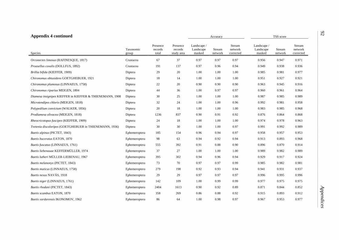
Appendix 4 continued Accuracy TSS score
Species Taxonomic group
Presence records
total
Presence records
study area
Landscape / Landscape
masked Stream network
Stream network corrected
Landscape / Landscape
masked Stream network
Stream network corrected
Orconectes limosus (RAFINESQUE, 1817) Crustacea 67 37 0.97 0.97 0.97 0.956 0.947 0.971
Proasellus coxalis (DOLLFUS, 1892) Crustacea 191 137 0.97 0.96 0.94 0.949 0.938 0.936
Brillia bifida (KIEFFER, 1909) Diptera 29 20 1.00 1.00 1.00 0.985 0.981 0.977
Chironomus obtusidens GOETGHEBUER, 1921 Diptera 18 14 1.00 1.00 1.00 0.951 0.927 0.921
Chironomus plumosus (LINNAEUS, 1758) Diptera 22 20 0.90 0.90 0.90 0.963 0.945 0.916
Chironomus riparius MEIGEN, 1804 Diptera 44 36 1.00 0.97 0.97 0.960 0.961 0.964
Diamesa insignipes KIEFFER in KIEFFER & THIENEMANN, 1908 Diptera 30 25 1.00 1.00 1.00 0.987 0.985 0.989
Microtendipes chloris (MEIGEN, 1818) Diptera 32 24 1.00 1.00 0.96 0.992 0.981 0.958
Polypedilum convictum (WALKER, 1856) Diptera 20 18 1.00 1.00 1.00 0.983 0.985 0.968
Prodiamesa olivacea (MEIGEN, 1818) Diptera 1236 837 0.90 0.91 0.92 0.876 0.864 0.868
Rheocricotopus fuscipes (KIEFFER, 1909) Diptera 24 18 1.00 1.00 1.00 0.974 0.978 0.963
Tvetenia discoloripes (GOETGHEBUER in THIENEMANN, 1936) Diptera 30 30 1.00 1.00 0.97 0.991 0.992 0.989
Baetis alpinus (PICTET, 1843) Ephemeroptera 185 154 0.96 0.94 0.97 0.958 0.957 0.953
Baetis buceratus EATON, 1870 Ephemeroptera 98 63 0.94 0.92 0.94 0.913 0.893 0.968
Baetis fuscatus (LINNAEUS, 1761) Ephemeroptera 555 392 0.91 0.88 0.90 0.896 0.870 0.914
Baetis liebenauae KEFFERMÜLLER, 1974 Ephemeroptera 37 27 1.00 1.00 1.00 0.989 0.982 0.989
Baetis lutheri MÜLLER-LIEBENAU, 1967 Ephemeroptera 395 302 0.94 0.96 0.94 0.929 0.917 0.924
Baetis melanonyx (PICTET, 1843) Ephemeroptera 73 70 0.97 0.97 0.99 0.985 0.982 0.981
Baetis muticus (LINNAEUS, 1758) Ephemeroptera 279 198 0.92 0.93 0.94 0.941 0.931 0.937
Baetis nexus NAVÁS, 1918 Ephemeroptera 29 29 0.97 0.97 0.97 0.996 0.995 0.996
Baetis niger (LINNAEUS, 1761) Ephemeroptera 142 109 1.00 0.99 0.99 0.977 0.975 0.975
Baetis rhodani (PICTET, 1843) Ephemeroptera 2404 1613 0.90 0.92 0.89 0.871 0.844 0.852
Baetis scambus EATON, 1870 Ephemeroptera 358 269 0.86 0.88 0.92 0.915 0.893 0.912
Baetis vardarensis IKONOMOV, 1962 Ephemeroptera 86 64 1.00 0.98 0.97 0.967 0.953 0.977
92
Appendices _______________________________________________________________________________________________________________________________________________________________________________

Appendix 4 continued Accuracy TSS score
Species Taxonomic group
Presence records
total
Presence records
study area
Landscape / Landscape
masked Stream network
Stream network corrected
Landscape / Landscape
masked Stream network
Stream network corrected
Baetis vernus CURTIS, 1834 Ephemeroptera 938 631 0.90 0.90 0.91 0.884 0.864 0.867
Caenis horaria (LINNAEUS, 1758) Ephemeroptera 161 47 0.77 0.70 0.72 0.923 0.913 0.929
Caenis luctuosa (BURMEISTER, 1839) Ephemeroptera 266 158 0.95 0.93 0.94 0.905 0.884 0.915
Caenis macrura STEPHENS, 1835 Ephemeroptera 116 78 0.91 0.91 0.99 0.948 0.931 0.964
Caenis rivulorum EATON, 1884 Ephemeroptera 74 63 0.81 0.84 0.92 0.942 0.966 0.926
Centroptilum luteolum (MÜLLER, 1776) Ephemeroptera 509 339 0.92 0.91 0.92 0.902 0.866 0.881
Cloeon dipterum (LINNAEUS, 1761) Ephemeroptera 154 87 0.89 0.88 0.88 0.923 0.881 0.931
Ecdyonurus dispar (CURTIS, 1834) Ephemeroptera 96 80 0.95 0.90 1.00 0.968 0.965 0.973
Ecdyonurus insignis (EATON, 1870) Ephemeroptera 29 26 0.96 0.92 1.00 0.984 0.974 0.985
Ecdyonurus macani THOMAS & SOWA, 1970 Ephemeroptera 29 24 1.00 1.00 1.00 0.991 0.993 0.988
Ecdyonurus submontanus LANDA, 1969 Ephemeroptera 38 30 1.00 1.00 1.00 0.976 0.984 0.982
Ecdyonurus torrentis KIMMINS, 1942 Ephemeroptera 285 238 0.92 0.96 0.96 0.953 0.944 0.946
Ecdyonurus venosus (FABRICIUS, 1775) Ephemeroptera 360 265 0.90 0.92 0.94 0.926 0.907 0.929
Electrogena affinis (EATON, 1883) Ephemeroptera 39 23 1.00 1.00 1.00 0.995 0.996 0.989
Electrogena ujhelyii (SOWA, 1981) Ephemeroptera 58 52 0.98 0.96 0.96 0.977 0.974 0.982
Epeorus assimilis EATON, 1885 Ephemeroptera 497 410 0.97 0.97 0.97 0.948 0.937 0.936
Epeorus sylvicola (PICTET, 1865) Ephemeroptera 57 32 1.00 1.00 1.00 0.987 0.981 0.981
Ephemera danica MÜLLER, 1764 Ephemeroptera 1179 750 0.90 0.94 0.91 0.867 0.851 0.842
Ephemera vulgata LINNAEUS, 1758 Ephemeroptera 51 17 0.76 0.76 0.88 0.925 0.907 0.969
Ephemerella mucronata (BENGTSSON, 1909) Ephemeroptera 373 290 0.94 0.93 0.96 0.946 0.935 0.931
Habroleptoides confusa SARTORI & JACOB, 1986 Ephemeroptera 629 455 0.95 0.93 0.95 0.931 0.922 0.925
Habroleptoides modesta (HAGEN, 1864) Ephemeroptera 14 13 1.00 1.00 1.00 0.999 0.999 0.995
Habrophlebia lauta EATON, 1884 Ephemeroptera 429 337 0.94 0.93 0.95 0.938 0.929 0.933
Heptagenia flava ROSTOCK, 1878 Ephemeroptera 92 44 0.89 0.93 1.00 0.960 0.961 0.963
Appendices
93 _______________________________________________________________________________________________________________________________________________________________________________

Appendix 4 continued Accuracy TSS score
Species Taxonomic group
Presence records
total
Presence records
study area
Landscape / Landscape
masked Stream network
Stream network corrected
Landscape / Landscape
masked Stream network
Stream network corrected
Heptagenia sulphurea (MÜLLER, 1776) Ephemeroptera 253 116 0.92 0.94 0.94 0.938 0.933 0.923
Oligoneuriella rhenana (IMHOFF, 1852) Ephemeroptera 24 17 1.00 1.00 1.00 0.992 0.991 0.988
Paraleptophlebia submarginata (STEPHENS, 1835) Ephemeroptera 221 154 0.97 0.96 0.94 0.944 0.933 0.935
Potamanthus luteus (LINNAEUS, 1767) Ephemeroptera 117 73 0.97 0.96 0.99 0.972 0.960 0.975
Procloeon bifidum (BENGTSSON, 1912) Ephemeroptera 93 62 0.95 0.97 0.97 0.968 0.962 0.968
Procloeon pennulatum (EATON, 1870) Ephemeroptera 16 15 1.00 1.00 1.00 0.988 0.974 0.984
Rhithrogena diaphana NAVÁS, 1917 Ephemeroptera 21 19 1.00 1.00 1.00 0.992 0.991 0.993
Rhithrogena germanica EATON, 1885 Ephemeroptera 19 19 0.95 1.00 1.00 0.995 0.995 0.979
Rhithrogena hercynia LANDA, 1969 Ephemeroptera 16 16 1.00 1.00 1.00 0.993 0.987 0.976
Rhithrogena picteti SOWA, 1971 Ephemeroptera 62 60 1.00 1.00 0.97 0.967 0.967 0.958
Rhithrogena puytoraci SOWA & DEGRANGE, 1987 Ephemeroptera 19 19 1.00 1.00 0.89 0.998 0.997 0.983
Rhithrogena semicolorata (CURTIS, 1834) Ephemeroptera 367 286 0.94 0.92 0.93 0.943 0.933 0.936
Serratella ignita (PODA, 1761) Ephemeroptera 1035 749 0.91 0.92 0.89 0.884 0.854 0.892
Torleya major (KLAPÁLEK, 1905) Ephemeroptera 535 356 0.97 0.97 0.94 0.937 0.931 0.919
Ancylus fluviatilis O.F. MÜLLER, 1774 Gastropoda 1484 1033 0.91 0.93 0.90 0.891 0.863 0.875
Anisus vortex (LINNAEUS, 1758) Gastropoda 151 46 0.91 0.91 0.93 0.931 0.912 0.951
Bithynia tentaculata (LINNAEUS, 1758) Gastropoda 555 292 0.95 0.92 0.93 0.908 0.881 0.906
Galba truncatula (O.F. MÜLLER, 1774) Gastropoda 72 51 0.90 0.88 0.88 0.941 0.895 0.893
Lymnaea stagnalis (LINNAEUS, 1758) Gastropoda 107 42 0.90 0.90 0.98 0.938 0.934 0.948
Physa fontinalis (LINNAEUS, 1758) Gastropoda 159 88 0.93 0.88 0.97 0.922 0.934 0.924
Physella acuta (DRAPARNAUD, 1805) Gastropoda 62 42 0.88 0.88 0.88 0.964 0.959 0.907
Planorbis planorbis (LINNAEUS, 1758) Gastropoda 61 21 0.90 0.90 0.90 0.957 0.948 0.956
Potamopyrgus antipodarum (GRAY, 1843) Gastropoda 754 483 0.95 0.95 0.95 0.902 0.892 0.886
Radix auricularia (LINNAEUS, 1758) Gastropoda 62 37 0.97 0.97 0.92 0.961 0.942 0.957
94
Appendices _______________________________________________________________________________________________________________________________________________________________________________
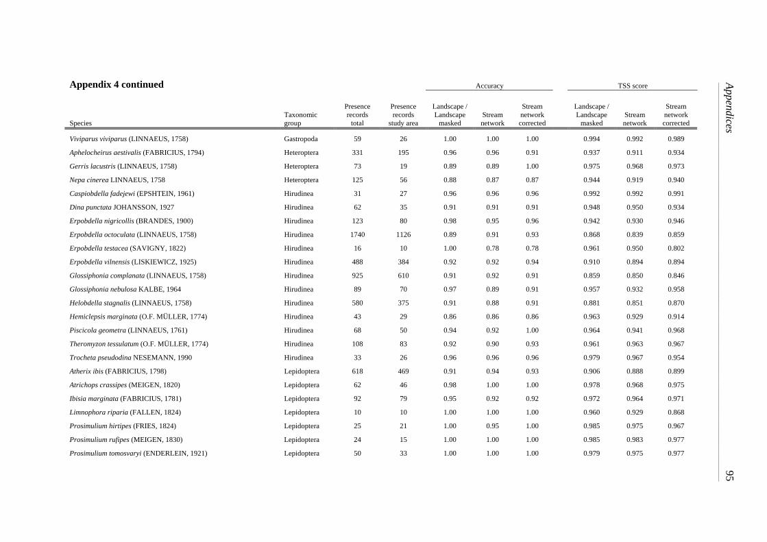
Appendix 4 continued Accuracy TSS score
Species Taxonomic group
Presence records
total
Presence records
study area
Landscape / Landscape
masked Stream network
Stream network corrected
Landscape / Landscape
masked Stream network
Stream network corrected
Viviparus viviparus (LINNAEUS, 1758) Gastropoda 59 26 1.00 1.00 1.00 0.994 0.992 0.989
Aphelocheirus aestivalis (FABRICIUS, 1794) Heteroptera 331 195 0.96 0.96 0.91 0.937 0.911 0.934
Gerris lacustris (LINNAEUS, 1758) Heteroptera 73 19 0.89 0.89 1.00 0.975 0.968 0.973
Nepa cinerea LINNAEUS, 1758 Heteroptera 125 56 0.88 0.87 0.87 0.944 0.919 0.940
Caspiobdella fadejewi (EPSHTEIN, 1961) Hirudinea 31 27 0.96 0.96 0.96 0.992 0.992 0.991
Dina punctata JOHANSSON, 1927 Hirudinea 62 35 0.91 0.91 0.91 0.948 0.950 0.934
Erpobdella nigricollis (BRANDES, 1900) Hirudinea 123 80 0.98 0.95 0.96 0.942 0.930 0.946
Erpobdella octoculata (LINNAEUS, 1758) Hirudinea 1740 1126 0.89 0.91 0.93 0.868 0.839 0.859
Erpobdella testacea (SAVIGNY, 1822) Hirudinea 16 10 1.00 0.78 0.78 0.961 0.950 0.802
Erpobdella vilnensis (LISKIEWICZ, 1925) Hirudinea 488 384 0.92 0.92 0.94 0.910 0.894 0.894
Glossiphonia complanata (LINNAEUS, 1758) Hirudinea 925 610 0.91 0.92 0.91 0.859 0.850 0.846
Glossiphonia nebulosa KALBE, 1964 Hirudinea 89 70 0.97 0.89 0.91 0.957 0.932 0.958
Helobdella stagnalis (LINNAEUS, 1758) Hirudinea 580 375 0.91 0.88 0.91 0.881 0.851 0.870
Hemiclepsis marginata (O.F. MÜLLER, 1774) Hirudinea 43 29 0.86 0.86 0.86 0.963 0.929 0.914
Piscicola geometra (LINNAEUS, 1761) Hirudinea 68 50 0.94 0.92 1.00 0.964 0.941 0.968
Theromyzon tessulatum (O.F. MÜLLER, 1774) Hirudinea 108 83 0.92 0.90 0.93 0.961 0.963 0.967
Trocheta pseudodina NESEMANN, 1990 Hirudinea 33 26 0.96 0.96 0.96 0.979 0.967 0.954
Atherix ibis (FABRICIUS, 1798) Lepidoptera 618 469 0.91 0.94 0.93 0.906 0.888 0.899
Atrichops crassipes (MEIGEN, 1820) Lepidoptera 62 46 0.98 1.00 1.00 0.978 0.968 0.975
Ibisia marginata (FABRICIUS, 1781) Lepidoptera 92 79 0.95 0.92 0.92 0.972 0.964 0.971
Limnophora riparia (FALLEN, 1824) Lepidoptera 10 10 1.00 1.00 1.00 0.960 0.929 0.868
Prosimulium hirtipes (FRIES, 1824) Lepidoptera 25 21 1.00 0.95 1.00 0.985 0.975 0.967
Prosimulium rufipes (MEIGEN, 1830) Lepidoptera 24 15 1.00 1.00 1.00 0.985 0.983 0.977
Prosimulium tomosvaryi (ENDERLEIN, 1921) Lepidoptera 50 33 1.00 1.00 1.00 0.979 0.975 0.977
Appendices
95 _______________________________________________________________________________________________________________________________________________________________________________

Appendix 4 continued Accuracy TSS score
Species Taxonomic group
Presence records
total
Presence records
study area
Landscape / Landscape
masked Stream network
Stream network corrected
Landscape / Landscape
masked Stream network
Stream network corrected
Simulium argyreatum MEIGEN, 1838 Lepidoptera 59 55 0.98 0.98 0.98 0.984 0.981 0.984
Simulium costatum FRIEDERICHS, 1920 Lepidoptera 21 18 1.00 1.00 1.00 0.960 0.960 0.957
Simulium cryophilum (RUBZOV, 1959) Lepidoptera 97 79 1.00 1.00 1.00 0.986 0.984 0.981
Simulium monticola FRIEDERICHS, 1920 Lepidoptera 27 23 1.00 1.00 0.96 0.978 0.969 0.976
Simulium ornatum MEIGEN, 1818 Lepidoptera 300 217 0.94 0.93 0.94 0.930 0.905 0.916
Simulium reptans (LINNAEUS, 1758) Lepidoptera 56 46 0.96 0.93 1.00 0.971 0.947 0.985
Simulium variegatum MEIGEN, 1818 Lepidoptera 54 41 0.95 0.95 0.98 0.984 0.971 0.987
Simulium vernum MACQUART, 1826 Lepidoptera 56 51 1.00 1.00 0.96 0.983 0.983 0.978
Sialis fuliginosa PICTET, 1836 Megaloptera 300 229 0.97 0.94 0.92 0.908 0.901 0.884
Sialis lutaria (LINNAEUS, 1758) Megaloptera 476 275 0.88 0.90 0.88 0.894 0.876 0.870
Sialis morio KLINGSTEDT, 1931 Megaloptera 22 21 1.00 1.00 1.00 1.000 0.999 0.999
Sialis nigripes PICTET, 1865 Megaloptera 34 27 0.93 0.96 0.96 0.956 0.942 0.984
Gordius aquaticus (LINNAEUS, 1758) Nematomorpha 30 30 0.97 1.00 0.93 0.985 0.982 0.956
Calopteryx splendens (HARRIS, 1782) Odonata 561 310 0.94 0.94 0.94 0.919 0.905 0.914
Calopteryx virgo (LINNAEUS, 1758) Odonata 173 121 0.94 0.93 0.95 0.919 0.897 0.924
Cordulegaster boltonii (DONOVAN, 1807) Odonata 51 45 1.00 0.98 0.93 0.976 0.975 0.959
Ischnura elegans (VAN DER LINDEN, 1820) Odonata 98 40 0.98 0.97 0.97 0.960 0.968 0.965
Platycnemis pennipes (PALLAS, 1771) Odonata 150 82 0.95 0.95 0.91 0.941 0.928 0.941
Eiseniella tetraedra (SAVIGNY, 1826) Oligochaeta 1149 870 0.91 0.93 0.89 0.896 0.866 0.873
Haplotaxis gordioides (HARTMANN, 1821) Oligochaeta 124 101 0.93 0.93 0.94 0.954 0.931 0.938
Limnodrilus hoffmeisteri CLAPAREDE, 1862 Oligochaeta 133 95 0.97 0.98 0.98 0.986 0.982 0.981
Limnodrilus profundicola (VERRILL, 1871) Oligochaeta 11 11 1.00 1.00 1.00 0.999 0.999 0.989
Lumbriculus variegatus (MÜLLER, 1774) Oligochaeta 418 314 0.96 0.96 0.95 0.908 0.911 0.898
Potamothrix hammoniensis (MICHAELSEN, 1901) Oligochaeta 33 19 1.00 1.00 1.00 0.990 0.993 0.993
96
Appendices _______________________________________________________________________________________________________________________________________________________________________________

Appendix 4 continued Accuracy TSS score
Species Taxonomic group
Presence records
total
Presence records
study area
Landscape / Landscape
masked Stream network
Stream network corrected
Landscape / Landscape
masked Stream network
Stream network corrected
Psammoryctides barbatus (GRUBE, 1891) Oligochaeta 94 61 0.97 0.98 0.95 0.974 0.973 0.972
Rhyacodrilus coccineus (VEJDOVSKÝ, 1875) Oligochaeta 23 16 1.00 1.00 1.00 0.975 0.992 0.960
Stylodrilus heringianus CLAPAREDE, 1862 Oligochaeta 439 338 0.96 0.96 0.93 0.918 0.895 0.906
Brachyptera risi (MORTON, 1896) Plecoptera 411 307 0.97 0.98 0.97 0.943 0.939 0.935
Brachyptera seticornis (KLAPÁLEK, 1902) Plecoptera 155 119 0.99 0.99 0.97 0.969 0.962 0.965
Chloroperla tripunctata (SCOPOLI, 1763) Plecoptera 12 12 1.00 1.00 1.00 0.998 0.988 0.976
Dinocras cephalotes (CURTIS, 1827) Plecoptera 95 87 0.89 0.99 0.92 0.977 0.972 0.972
Diura bicaudata (LINNAEUS, 1758) Plecoptera 30 20 1.00 0.89 1.00 0.955 0.936 0.944
Isoperla grammatica (PODA, 1761) Plecoptera 42 27 0.96 0.96 0.96 0.986 0.980 0.979
Leuctra braueri KEMPNY, 1898 Plecoptera 17 16 1.00 1.00 1.00 0.995 0.993 0.974
Leuctra geniculata (STEPHENS, 1836) Plecoptera 196 170 0.96 0.96 0.96 0.958 0.946 0.957
Nemurella pictetii KLAPÁLEK, 1900 Plecoptera 47 39 1.00 1.00 1.00 0.964 0.958 0.974
Perla marginata (PANZER, 1799) Plecoptera 180 142 0.92 0.94 0.96 0.969 0.965 0.960
Perlodes microcephalus (PICTET, 1833) Plecoptera 48 38 0.97 0.97 1.00 0.982 0.971 0.984
Hypania invalida (GRUBE, 1860) Polychaeta 36 26 1.00 1.00 1.00 0.978 0.983 0.973
Ephydatia fluviatilis (LINNAEUS, 1758) Porifera 45 23 0.96 0.95 1.00 0.911 0.878 0.990
Spongilla lacustris (LINNAEUS, 1758) Porifera 35 19 0.95 0.95 0.95 0.977 0.981 0.988
Trochospongilla horrida WELTNER, 1893 Porifera 13 12 1.00 1.00 1.00 1.000 1.000 1.000
Adicella reducta (McLACHLAN, 1865) Trichoptera 82 68 1.00 1.00 1.00 0.944 0.937 0.958
Agapetus fuscipes CURTIS, 1834 Trichoptera 70 59 0.98 0.98 0.98 0.956 0.943 0.955
Agapetus ochripes CURTIS, 1834 Trichoptera 46 31 0.97 1.00 1.00 0.975 0.967 0.987
Allogamus auricollis (PICTET, 1834) Trichoptera 110 88 0.93 0.95 0.98 0.966 0.949 0.968
Annitella obscurata (McLACHLAN, 1876) Trichoptera 36 36 0.97 0.97 0.97 0.964 0.957 0.968
Anomalopterygella chauviniana (STEIN, 1874) Trichoptera 495 417 0.94 0.94 0.96 0.942 0.933 0.935
Appendices
97 _______________________________________________________________________________________________________________________________________________________________________________

Appendix 4 continued Accuracy TSS score
Species Taxonomic group
Presence records
total
Presence records
study area
Landscape / Landscape
masked Stream network
Stream network corrected
Landscape / Landscape
masked Stream network
Stream network corrected
Athripsodes albifrons (LINNAEUS, 1758) Trichoptera 136 103 0.98 0.98 0.96 0.960 0.955 0.944
Athripsodes cinereus (CURTIS, 1834) Trichoptera 277 171 0.94 0.95 0.94 0.918 0.894 0.924
Brachycentrus subnubilus CURTIS, 1834 Trichoptera 145 93 0.97 0.99 0.95 0.944 0.930 0.960
Ceraclea annulicornis (STEPHENS, 1836) Trichoptera 26 18 1.00 1.00 1.00 0.970 0.971 0.987
Ceraclea dissimilis (STEPHENS, 1836) Trichoptera 98 49 1.00 0.96 0.88 0.949 0.919 0.938
Chaetopterygopsis maclachlani STEIN, 1874 Trichoptera 22 21 1.00 1.00 1.00 0.996 0.996 0.986
Cheumatopsyche lepida (PICTET, 1834) Trichoptera 158 94 0.97 0.96 0.98 0.951 0.935 0.958
Cyrnus trimaculatus (CURTIS, 1834) Trichoptera 144 102 0.90 0.91 0.91 0.951 0.934 0.946
Drusus annulatus (STEPHENS, 1837) Trichoptera 206 163 0.98 0.98 0.96 0.950 0.936 0.949
Ecclisopteryx dalecarlica KOLENATI, 1848 Trichoptera 52 42 0.98 0.98 0.95 0.981 0.968 0.967
Ecclisopteryx madida (McLACHLAN, 1867) Trichoptera 35 28 0.96 0.96 0.96 0.981 0.982 0.984
Glossosoma boltoni CURTIS, 1834 Trichoptera 28 27 1.00 1.00 1.00 0.989 0.985 0.993
Glossosoma conformis NEBOISS, 1963 Trichoptera 79 63 0.98 0.95 0.97 0.975 0.966 0.966
Goera pilosa (FABRICIUS, 1775) Trichoptera 236 173 0.97 0.94 0.94 0.906 0.888 0.923
Halesus radiatus (CURTIS, 1834) Trichoptera 299 153 0.98 0.98 0.94 0.927 0.910 0.897
Halesus tesselatus (RAMBUR, 1842) Trichoptera 48 29 1.00 1.00 1.00 0.978 0.976 0.947
Hydropsyche bulbifera McLACHLAN, 1878 Trichoptera 45 22 1.00 1.00 1.00 0.991 0.987 0.987
Hydropsyche dinarica MARINKOVIC, 1979 Trichoptera 143 126 0.98 0.98 0.93 0.966 0.961 0.962
Hydropsyche fulvipes (CURTIS, 1834) Trichoptera 19 19 1.00 1.00 1.00 0.979 0.988 0.992
Hydropsyche guttata PICTET, 1834 Trichoptera 14 14 0.93 1.00 0.93 0.969 0.964 0.940
Hydropsyche incognita PITSCH, 1993 Trichoptera 305 244 0.93 0.94 0.90 0.925 0.904 0.933
Hydropsyche instabilis (CURTIS, 1834) Trichoptera 444 357 0.92 0.92 0.95 0.917 0.905 0.900
Hydropsyche pellucidula (CURTIS, 1834) Trichoptera 700 457 0.90 0.91 0.91 0.872 0.835 0.876
Hydropsyche saxonica McLACHLAN, 1884 Trichoptera 262 180 0.95 0.94 0.93 0.913 0.898 0.925
98
Appendices _______________________________________________________________________________________________________________________________________________________________________________

Appendix 4 continued Accuracy TSS score
Species Taxonomic group
Presence records
total
Presence records
study area
Landscape / Landscape
masked Stream network
Stream network corrected
Landscape / Landscape
masked Stream network
Stream network corrected
Hydropsyche siltalai DÖHLER, 1963 Trichoptera 1442 990 0.91 0.92 0.90 0.886 0.859 0.868
Hydropsyche tenuis NAVÁS, 1932 Trichoptera 39 35 0.97 0.94 0.94 0.988 0.988 0.987
Lepidostoma hirtum (FABRICIUS, 1775) Trichoptera 517 375 0.91 0.91 0.95 0.911 0.890 0.910
Limnephilus lunatus CURTIS, 1834 Trichoptera 324 115 0.91 0.92 0.86 0.929 0.921 0.905
Limnephilus marmoratus CURTIS, 1834 Trichoptera 21 20 1.00 1.00 0.95 0.985 0.981 0.978
Lithax niger (HAGEN, 1859) Trichoptera 33 25 1.00 1.00 1.00 0.967 0.941 0.971
Lype phaeopa (STEPHENS, 1836) Trichoptera 20 19 1.00 1.00 1.00 0.975 0.960 0.958
Lype reducta (HAGEN, 1868) Trichoptera 105 66 0.94 0.91 0.86 0.970 0.956 0.930
Micrasema longulum McLACHLAN, 1876 Trichoptera 147 112 0.98 0.98 0.99 0.963 0.956 0.961
Micrasema minimum McLACHLAN, 1876 Trichoptera 91 67 0.99 0.99 0.99 0.983 0.980 0.979
Molanna angustata CURTIS, 1834 Trichoptera 67 23 0.96 0.96 1.00 0.957 0.942 0.961
Mystacides azurea (LINNAEUS, 1761) Trichoptera 341 271 0.94 0.92 0.94 0.917 0.910 0.907
Mystacides nigra (LINNAEUS, 1758) Trichoptera 99 66 0.92 0.91 0.94 0.955 0.924 0.963
Odontocerum albicorne (SCOPOLI, 1763) Trichoptera 390 304 0.95 0.95 0.95 0.934 0.918 0.921
Oecetis notata (RAMBUR, 1842) Trichoptera 32 21 0.86 0.86 0.90 0.952 0.935 0.928
Oecetis testacea (CURTIS, 1834) Trichoptera 63 53 0.96 0.96 0.91 0.966 0.958 0.978
Philopotamus ludificatus McLACHLAN, 1878 Trichoptera 39 32 1.00 1.00 1.00 0.977 0.961 0.982
Psychomyia pusilla (FABRICIUS, 1781) Trichoptera 381 261 0.93 0.93 0.91 0.921 0.897 0.918
Rhyacophila evoluta McLACHLAN, 1879 Trichoptera 119 102 0.99 0.99 0.98 0.973 0.969 0.970
Rhyacophila nubila (ZETTERSTEDT, 1840) Trichoptera 329 257 0.97 0.96 0.97 0.928 0.931 0.950
Rhyacophila obliterata McLACHLAN, 1863 Trichoptera 62 50 1.00 0.98 0.98 0.951 0.942 0.951
Rhyacophila pubescens PICTET, 1834 Trichoptera 11 10 0.90 0.90 0.90 0.978 0.992 0.967
Rhyacophila torrentium PICTET, 1834 Trichoptera 28 26 1.00 1.00 1.00 0.983 0.986 0.954
Rhyacophila tristis PICTET, 1834 Trichoptera 77 63 0.97 1.00 1.00 0.972 0.957 0.970
Appendices
99 _______________________________________________________________________________________________________________________________________________________________________________

Appendix 4 continued Accuracy TSS score
Species Taxonomic group
Presence records
total
Presence records
study area
Landscape / Landscape
masked Stream network
Stream network corrected
Landscape / Landscape
masked Stream network
Stream network corrected
Sericostoma flavicorne SCHNEIDER, 1845 Trichoptera 57 57 1.00 1.00 0.98 0.988 0.984 0.982
Sericostoma personatum KIRBY & SPENCER, 1826 Trichoptera 162 126 0.98 0.97 0.97 0.965 0.951 0.956
Silo pallipes (FABRICIUS, 1781) Trichoptera 311 237 0.97 0.97 0.96 0.949 0.937 0.935
Silo piceus (BRAUER, 1857) Trichoptera 194 153 0.91 0.92 0.95 0.947 0.940 0.944
Tinodes rostocki McLACHLAN, 1878 Trichoptera 33 27 1.00 1.00 1.00 0.974 0.977 0.985
Dendrocoelum lacteum (O.F. MÜLLER, 1774) Turbellaria 210 158 0.97 0.94 0.95 0.940 0.908 0.933
Dugesia gonocephala (DUGES, 1830) Turbellaria 716 555 0.94 0.91 0.92 0.905 0.882 0.889
Dugesia lugubris (SCHMIDT, 1861) Turbellaria 116 85 0.89 0.91 0.92 0.946 0.917 0.954
Dugesia polychroa (SCHMIDT, 1861) Turbellaria 16 15 1.00 1.00 0.93 0.997 0.996 0.989
Dugesia tigrina (GIRARD, 1850) Turbellaria 86 69 0.91 0.89 0.95 0.967 0.957 0.968
Polycelis felina (DALYELL, 1814) Turbellaria 120 109 0.95 0.94 0.96 0.978 0.980 0.980
Polycelis nigra MUELLER, 1774 Turbellaria 88 77 0.83 0.78 0.81 0.949 0.932 0.881
100
Appendices _______________________________________________________________________________________________________________________________________________________________________________

Appendices 101
Appendix 5 Pairwise percent (± standard deviations) of overlapping grid cells classified as suit-able between all combinations of the four modelling designs.
Landscape Landscape masked Stream network
Landscape masked 51 ± 20%
Stream network 45 ± 5% 93 ± 7%
Stream network corrected 36 ± 6% 74 ± 15% 77 ± 15%

102 Author contributions
Author contributions
Chapter 1
Climate-change winners and losers: stream macroinvertebrates of a submontane
region in Central Europe
Sami Domisch, Sonja C. Jähnig, Peter Haase (2011). Freshwater Biology 56, 2009–
2020
S.D., S.C.J. and P.H. conceived the research. S.D. conducted the research, analysed the
data, and wrote the manuscript. All authors discussed the results and commented on the
manuscript. S.C.J. and P.H. contributed equally to the study. Two anonymous referees
commented on the manuscript.
Chapter 2
How would climate change affect European stream macroinvertebrates’
distributions?
Sami Domisch, Miguel B. Araújo, Núria Bonada, Steffen U. Pauls, Sonja C. Jähnig,
Peter Haase. Submitted to Global Change Biology
S.D., S.C.J. and P.H. conceived the research. S.D. conducted the research, analysed the
data and wrote the manuscript. M.B.A., N.B., and S.U.P. contributed species data. All
authors discussed the results and commented on the manuscript. S.C.J. and P.H. con-
tributed equally to the study.
Chapter 3
Choice of study area and predictors affect species distribution models of
stream macroinvertebrates
Sami Domisch, Mathias Kuemmerlen, Sonja C. Jähnig, Peter Haase. Submitted to
Freshwater Biology
S.D., M.K., S.C.J. and P.H. conceived the research. S.D. conducted the research, ana-
lysed the data, and wrote the manuscript. All authors discussed the results and com-
mented on the manuscript. S.C.J. and P.H. contributed equally to the study.

Acknowledgements 103
Acknowledgements
This thesis could not have been accomplished without the help of many people who
have supported me throughout the time of my dissertation. First of all I wish to thank
my supervisors Peter Haase and Sonja Jähnig for both guiding me around the obstacles
of a PhD project, and similarly giving me the space to develop and apply my own ideas.
Further, I am grateful to Oliver Tackenberg for support and for reviewing the thesis.
I wish to thank a number of scientists from various fields, from whom I have received
valuable support during my research: Stefan Stoll, Carsten Nowak, Miklós Bálint,
Steffen Pauls, Heike Kappes, Andrea Sundermann, Jürgen Jung, Jana Schröder, as well
as Núria Bonada and Miguel Araújo for help, data, fruitful discussions and valuable
comments during the last three years. I greatly acknowledge Karin Boos’ help in lin-
guistic revisions.
I am grateful to all my colleagues of the working group in Gelnhausen for sharing the
burden of mastering this thesis. Especially I wish to thank Joao Barateiro Diogo,
Kathrin Steyer, Christiane Frosch, Verena Harms, Jan Sauer, Sabrina Nemec, Anna
Ernst, Mascha Siemund, Jutta Geismar, Deep-Narayan and Ram Devi Tachamo Shah,
Miriam Gerhardt, Franziska Zeuner, Jan Außem, Annakarina Mundorf, and Philipp Olt.
Most of all, I want to thank Denise Früh and Mathias Kuemmerlen for being there, lots
of discussions, and invaluable help in solving all kinds of problems that occurred during
the PhD research. It has really been a pleasure working with you!
Further, I am grateful to Jonathan Heubes, Sarah Cunze, Svenja Meierfrankenfeld, Ma-
ren Ziegler, Marion Leiblein, Katja Heubach, Konstantin König, and Jaime Garcia for
fruitful discussions, as well as valuable support with GIS and R.
I wish to thank my family, my parents Rainer and Maila Domisch, and my brothers and
sister Timo, Nina, and Mika Domisch for your permanent support all the time. This
work is dedicated to my father. Thank you for your endless support and motivation, and
for never being tired of guiding me. Your positive attitude kept me going.
Most, I want to thank Connie Plagge for being there for me, for your love and your pa-
tience.

104 Acknowledgements
The support of the Umweltbundesamt (UBA), the Hessisches Landesamt für Umwelt
und Geologie (HLUG), the Landesamt für Umwelt, Messungen und Naturschutz Baden-
Württemberg (LUBW), and the Deutscher Wetterdienst (DWD) is greatly acknowl-
edged for providing data during my research, respectively. Further, I want to thank the
Environmental Systems Research Institute (ESRI) for providing the ArcGIS software,
and the German Academic Exchange Service (DAAD) for providing travel funds. This
thesis was financially supported by the research funding programme ‘LOEWE – Lan-
des-Offensive zur Entwicklung Wissenschaftlich-ökonomischer Exzellenz’ of Hesse’s
Ministry of Higher Education, Research, and the Arts.

105
Erklärung
Ich erkläre hiermit, dass ich mich bisher keiner Doktorprüfung unterzogen habe.
Frankfurt am Main, den .................................. ………………………………..............
(Unterschrift)
Eidesstattliche Versicherung
Ich erkläre hiermit an Eides Statt, dass ich die vorgelegte Dissertation über
Species distribution modelling of stream macroinvertebrates under climate
change scenarios
selbständig angefertigt und mich anderer Hilfsmittel als der in ihr angegebenen nicht
bedient habe, insbesondere, dass alle Entlehnungen aus anderen Schriften mit Angabe
der betreffenden Schrift gekennzeichnet sind.
Ich versichere, nicht die Hilfe einer kommerziellen Promotionsvermittlung in Anspruch
genommen zu haben.
Frankfurt am Main, den ............................... …...............…………………………..
(Unterschrift)

106
Curriculum Vitae
Dipl.-Biol. Sami Domisch
Personal Details
Name: Sami Jan-Henrik Domisch
Date of birth: March 9, 1982
Place of birth: Helsinki, Finland
Nationality: Finnish / German
Residence: Gartenstr. 145
D-60596 Frankfurt am Main
Germany
Education
Since 2009 Senckenberg Research Institutes and Natural History Museums, Biodi-
versity and Climate Research Centre (BiK-F), Frankfurt, Germany: PhD
research under the supervision of Prof. Dr. P. Haase and Dr. S. Jähnig
2007-2008 Marine Station of the Alfred-Wegener-Institute for Polar and Marine
Research, AWI, Helgoland, Germany: Diploma thesis under the supervi-
sion of Dr. M. Molis: „Effekte des eingewanderten Japanischen Beeren-
tangs Sargassum muticum (Yendo) Fensholt auf die Diversität und Struk-
tur makrobenthischer Gemeinschaften im Helgoländer Felswatt“ (“Ef-
fects of Sargassum muticum on the structure and diversity of macroben-
thic rocky shore communities at Helgoland”)
2005-2007 Carl von Ossietzky Universität Oldenburg, Germany: Advanced studies
in biology, main focus: Ecology, Zoology, Plant physiology, Marine bio-
diversity
2001-2005 Technische Universität Kaiserslautern, Germany: Basic studies in biolo-
gy
2000 Reifeprüfung at the Deutsche Schule Helsinki, Finland

107
Publications
Articles
Bálint, M., Domisch, S., Engelhardt, C.H.M., Haase, P., Lehrian, S., Sauer, J.,
Theissinger, K., Pauls, S.U., Nowak, C. (2011). Cryptic biodiversity loss linked to
global climate change. Nature Climate Change, 1, 313–318
Domisch, S., Jähnig. S.C., Haase, P. (2011). Climate-change winners and losers: stream
macroinvertebrates of a submontane region in Central Europe. Freshwater Biol-
ogy, 56, 2009-2020
Sauer, J., Domisch, S., Nowak, C., Haase, P. (2011). Low mountain ranges: summit
traps for montane freshwater species under climate change. Biodiversity and Con-
servation, 20, 3133-3146
Kuemmerlen, M., Domisch, S., Schmalz, B., Cai, Q., Fohrer, N., Jähnig, S.C. (2012).
Integrierte Modellierung von aquatischen Ökosystemen in China: Arealbestim-
mung von Makrozoobenthos auf Einzugsgebietsebene. Hydrologie und Wasser-
bewirtschaftung, in press
Domisch, S., Kuemmerlen, M., Jähnig, S.C., Haase, P. Choice of study area and predic-
tors affects species distribution models of stream macroinvertebrates. Freshwater
Biology, submitted
Domisch, S., Araújo, M.B., Bonada, N., Pauls, S.U., Jähnig, S.C., Haase, P. How would
climate change affect European stream macroinvertebrates’ distributions? Global
Change Biology, submitted
Tachamo Shah, R.D., Narayan-Shah, D., Domisch, S. Range shifts of a relict Himalayan
dragonfly in the Hindu Kush Himalayan region under climate change scenarios.
International Journal of Odonatology, submitted
Jähnig, S., Domisch, S., Kuemmerlen, M., Schmalz, B., Kiesling J., Fohrer N., Cai, Q.
Modelling of riverine ecosystems by integrating models: conceptual approach, a
case study and research agenda. Journal of Biogeography, submitted
Further publications
Novak, C., Bálint, M. Liebrich, A., Domisch, S., Sauer, J., Bauer, M., Früh, D., Geis-
mar, J., Nemec, S., Wittig R., Haase, P., Pauls, S.U. (2011). Assessing the fate of
montane biodiversity in Europe under Climate Change – a novel approach using
species distribution modeling and population genetics. BfN Europäische For-

108
schungskonferenz Biologische Vielfalt und Klimawandel. Zusammenfassungen
der Jahrestagung 2011, Bonn, Germany.
Sauer, J., Bálint, M., Domisch, S., Nowak, C, Haase, P. (2010). Modellierung klimabe-
dingter Nischenverschiebung bei montanen aquatischen Insekten. BfN-
Statuskonferenz. Zusammenfassungen der Jahrestagung 2010, Bonn, Germany
Domisch, S., Jähnig, S. C., Haase, P. (2010). Modellierung klimabedingter Arealver-
schiebungen ausgewählter Makrozoobenthosarten. Deutsche Gesellschaft für
Limnologie (DGL). Erweiterte Zusammenfassungen der Jahrestagung 2009, Ol-
denburg, Germany
Talks
Domisch, S., Jähnig. S., Haase, P. (2011). Modellierung klimabedingter Arealverschie-
bungen von Makrozoobenthosarten auf verschiedenen räumlichen Skalen. Jahres-
tagung der Deutschen Gesellschaft für Limnologie, 12. – 16. September 2011,
Weihenstephan, Germany.
Pauls, S.U., Bálint, M., Domisch, S., Engelhardt, C.H.M., Haase, P., Lehrian, S., Sauer,
J., Theissinger, K., Nowak, C. Assessing losses of genetic diversity in aquatic in-
sects under climate change scenarios, 12. – 16. September 2011, Weihenstephan,
Germany.
Bálint, M., Domisch, S., Engelhardt, C.H.M., Haase, P., Lehrian, S., Sauer, J., Theissin-
ger, K., Pauls, S.U., Nowak, C. (2011). Climate change will lead to massive loss
of genetic and cryptic diversity. 7th Symposium for European Freshwater Sci-
ences, 26. June – 01. July 2011, Girona, Spain.
Domisch, S., Jähnig. S., Haase, P. (2011). Species distribution modeling of stream in-
vertebrates under climate change scenarios. 7th Symposium for European Fresh-
water Sciences, 26. June – 01. July 2011, Girona, Spain.
Jähnig, S., Gies M., Domisch, S., Früh. D., Hering, D., Haase, P. (2011). A trait-based
approach to assess climate change effects on stream biota. Annual Meeting of the
North American Benthological Society, 22. – 26. May 2011, Providence, Rhode
Island, USA.
Nowak, C., Bálint, M. Liebrich, A., Domisch, S., Sauer, J., Bauer, M., Früh, D., Geis-
mar, J., Nemec, S., Wittig R., Haase, P., Pauls, S.U. (2011) Assessing the fate of
montane biodiversity in Europe under Climate Change – a novel approach using
species distribution modeling and population genetics. BfN Europäische For-

109
schungskonferenz Biologische Vielfalt und Klimawandel. 12. – 14 April 2011,
Bonn, Germany.
Domisch, S. (2010). Species distribution modelling of freshwater invertebrates. Biof-
resh – Climate change and invasives modelling meeting, 12. – 14. July 2010, Tou-
louse, France.
Sauer, J., Bálint, M., Domisch, S., Nowak, C, Haase, P. (2010). Modellierung klimabe-
dingter Nischenverschiebung bei montanen aquatischen Insekten. BfN Statuskon-
ferenz „Biologische Vielfalt und Klimawandel“, 02. – 03. March 2010, Bonn,
Germany.
Domisch, S., Molis, M. (2007). Effects of Sargassum muticum on the structure and di-
versity of macrobenthic rocky shore communities at Helgoland. 42nd European
Marine Biology Symposium, 27. – 31. August 2007, Kiel, Germany.
Poster presentations
Shah, R.D.T., Domisch, S., Shah, D.N. (2012) Human pressure constricting the suitable
habitat: A case study of a relict Himalayan dragonfly in the Hindu Kush Himala-
yan region. Planet Under Pressure Conference, 26. – 29. March 2012, London,
UK.
Domisch, S., Jähnig, S.C., Haase, P. (2009). Modellierung klimabedingter Arealver-
schiebungen ausgewählter Makrozoobenthosarten. Jahrestagung der Deutschen
Gesellschaft für Limnologie, 28. September – 02. October 2009, Oldenburg, Ger-
many.
![Modelling species distributions without using species ...webpages.icav.up.pt/PTDC/BIA-BEC/105093/2008/most_revel/[A].pdf · Modelling species distributions without using species distributions:](https://img.pdfslide.net/doc/110x75/5b31859e7f8b9ab5728c37a7/modelling-species-distributions-without-using-species-apdf-modelling-species.jpg)