Specification and Analysis of Real-time Problem Solvers

Babak HamidzadehShashi Shekhar

Computer Science Dept.University of MinnesotaMinneapolis, MN 55455

ABSTRACT

There has been a recent rise in research on real-time problem solving algo-rithms in artificial intelligence (AI). A real-time AI problem solver performs atask or a set of tasks in two phases. During the first phase, the problem solversearches for a solution that, once executed, will satisfy the requirements of thetask. We refer to this phase as the planning phase or the search phase. Duringthe next phase, the problem solver executes the planned solution to achieve thedesired results of the task. This phase is referred to as the execution phase.Under time constraints, a real-time AI problem solver must balance planningand execution to minimize total response times and to comply with deadlines.This paper provides a methodology for the specification of real-time AI problemsolvers. Using this methodology, we provide a formal specification of a real-time problem. In addition, the paper presents a methodology for analyzing real-time AI problem solvers. This methodology is demonstrated via a case study oftwo real-time problem solvers, namely DYNORAII and RTA*[ 1], for the real-time path planning problem. We provide new results on worst-case andaverage-case complexity of the problem, and of the algorithms that solve it. Wealso provide experimental evaluation of DYNORAII and RTA* for deadlinecompliance and response-time minimization.

Index Terms: Real-time, Problem Solving, Search.

− 2 −

1. Introduction

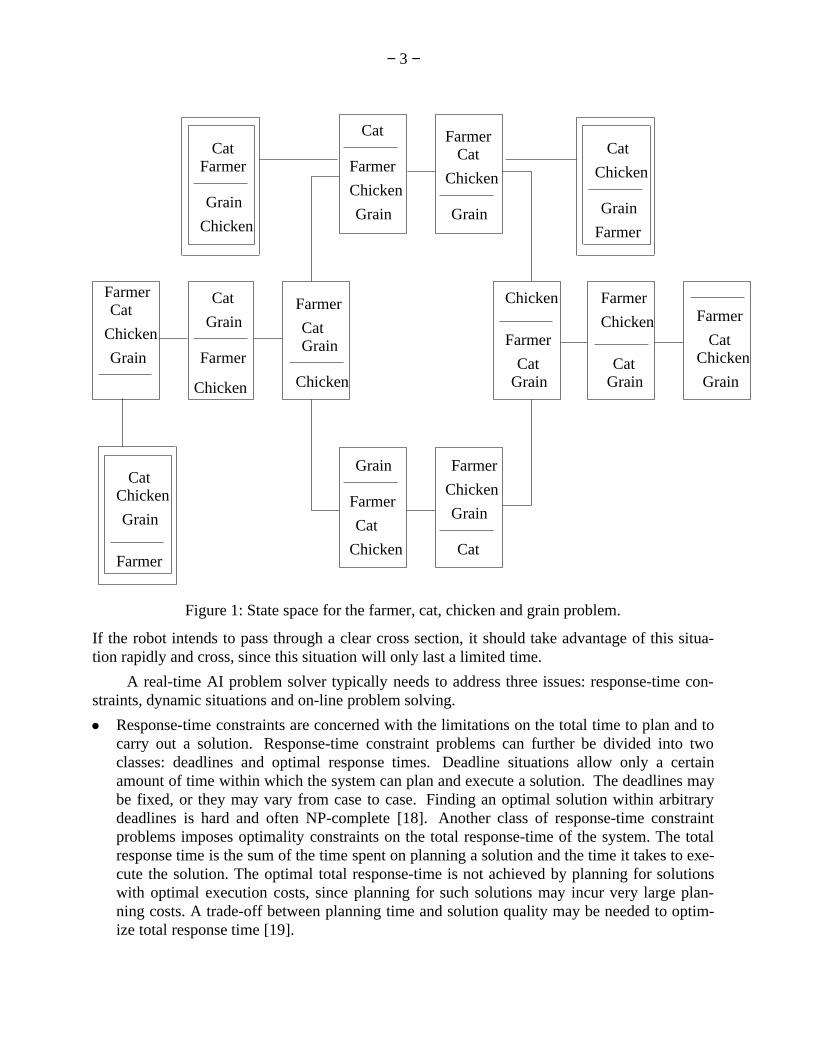
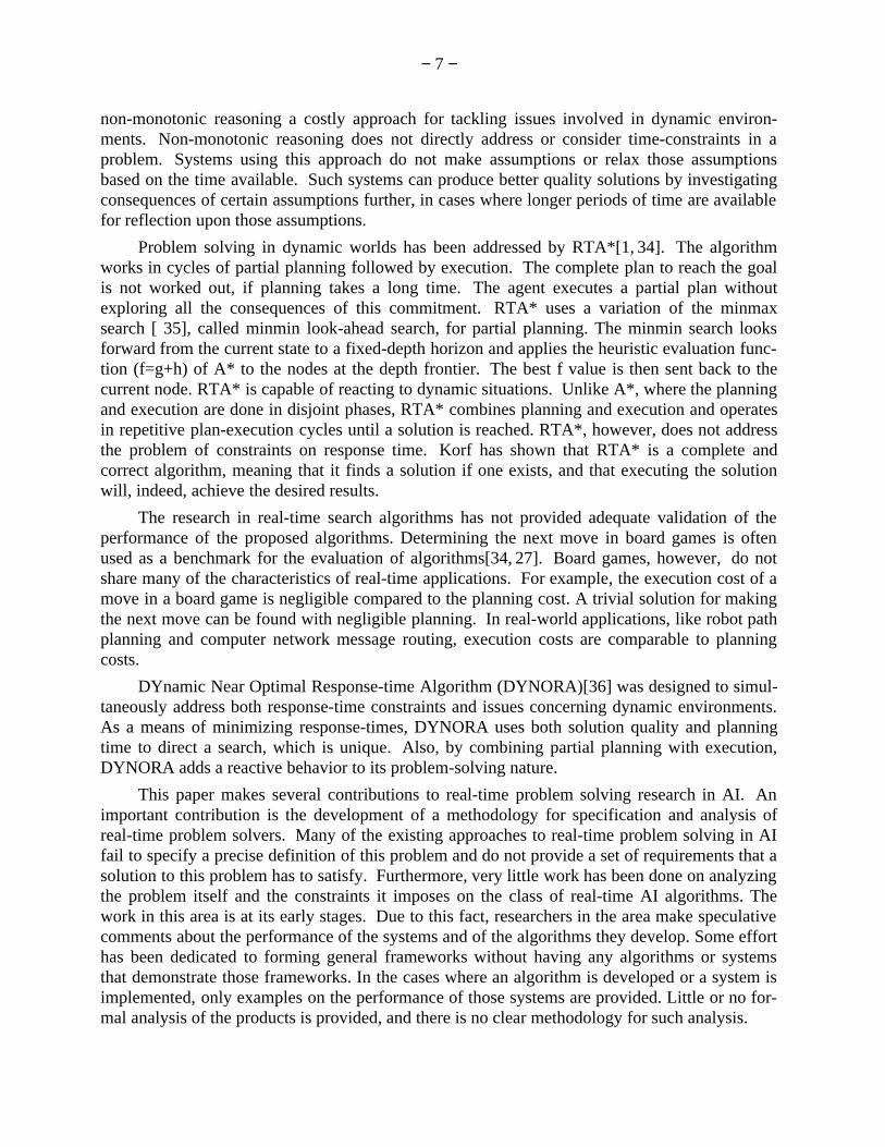
A problem solver in AI consists of three main components, namely a global data base, a setof transition rules and a control system[2]. The global data base contains statements and datathat reflect the state of the world at each point in time. The transition rules operate on the globaldata base. Each rule has a set of preconditions that must be satisfied by the state represented inthe global data base before that rule can be applied. Application of a rule changes the globaldata base to represent a new world state. The control system has the task of reaching a desiredstate or a goal state, via choosing and ordering a set of rules, such that application of those rulesin the specified order will transform the global data base from its initial state to the goal state.The set of all possible states and all possible transitions from one state to another is referred to asthe state space. The state space of a problem can be represented as a graph in which the nodesrepresent the states and the edges represent transitions. A control system in this representationcan be characterized as a search process that seeks a sequence of state transitions that forms apath in the state space, connecting the start state to the goal state.

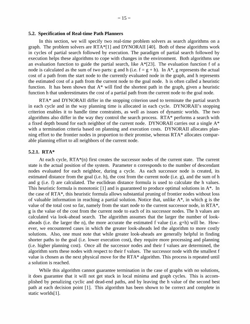
An example state space for the farmer, cat, chicken and grain problem is shown in figure 1.In this problem, a farmer has to take his cat, chicken and grain safely across a river[3]. The riveris represented by the line across a node in the state space graph. The farmer can neither leave thechicken and the grain nor the cat and the chicken at one end by themselves, as one will eat theother. A move from one side of the river to another is represented by an edge connecting twonodes, which represent the state before the move and the state after the move. Some of theunsafe states in the state space are demonstrated by the states enclosed by a double line in thefigure.

A real-time AI problem solver has to operate under certain time constraints imposed on itby the environment. The control system of a real-time AI problem solver has to perform itssearch process in such a way that the temporal constraints of the problem are satisfied. In thegame of lightning chess, for example, the problem solver has to search for a move in the statespace, within a time limit. Any amount of time saved within a move can be used in later moves.Thus, the lightning chess problem solver has to produce responses by the time the deadlinearrives. Ideally, the problem solver seeks to produce a response in less time than that allowed bythe deadline, in order to buy time for more complicated decision problems to come.

Real-time AI problem solvers differ from conventional real-time systems. Conventionalreal-time systems [4, 5, 6] are mainly concerned with static tasks in which much of the informa-tion about the task is known a priori. These systems have mainly addressed the problem ofmeeting fixed deadlines. These conventional systems have focused on issues related to schedul-ing of tasks [4, 6, 5, 7, 7], interrupt and error handling [8], communication requirements[9, 10, 11] and system design and analysis [12, 13, 14, 15, 16, 17]. In addition to the above issues,real-time AI problem solvers aim at handling other constraints in the environment, such asuncertainty and lack of complete knowledge about the environment, dynamicity in the world,bounded validity time of information and other resource constraints. Consider, for example, thedynamic scenario in which a robot is among a set of moving agents with missions of their own.These agents are expected to move according to a set of traffic laws, but they do not always doso. A situation in which response-time constraints become important, in this scenario, is whenthe robot has to go from one point to the other within a deadline (global deadline). In this situa-tion, while the robot has to react to changes to avoid collisions, it must plan a route and executeit within a certain time. The robot only has a limited time to react to changes (local deadlines).

− 3 −

Farmer

Grain

ChickenCat

Farmer

Grain

Chicken

Cat

Cat

CatCat

Cat

Cat

Cat

Cat

Cat

Chicken

Chicken

Chicken

Chicken

Chicken

ChickenChicken

ChickenChicken GrainGrainGrain

Grain

Grain

GrainGrain

Grain

Grain

Cat

Farmer

FarmerFarmer

Farmer

Farmer

Farmer

Farmer

Farmer

Farmer

Cat

Chicken

Grain

Farmer

Farmer

Grain

Chicken

Cat

Figure 1: State space for the farmer, cat, chicken and grain problem.

If the robot intends to pass through a clear cross section, it should take advantage of this situa-tion rapidly and cross, since this situation will only last a limited time.

A real-time AI problem solver typically needs to address three issues: response-time con-straints, dynamic situations and on-line problem solving.

g Response-time constraints are concerned with the limitations on the total time to plan and tocarry out a solution. Response-time constraint problems can further be divided into twoclasses: deadlines and optimal response times. Deadline situations allow only a certainamount of time within which the system can plan and execute a solution. The deadlines maybe fixed, or they may vary from case to case. Finding an optimal solution within arbitrarydeadlines is hard and often NP-complete [18]. Another class of response-time constraintproblems imposes optimality constraints on the total response-time of the system. The totalresponse time is the sum of the time spent on planning a solution and the time it takes to exe-cute the solution. The optimal total response-time is not achieved by planning for solutionswith optimal execution costs, since planning for such solutions may incur very large plan-ning costs. A trade-off between planning time and solution quality may be needed to optim-ize total response time [19].

− 4 −

g Dynamic situations are those in which the world changes slowly during planning. The longerthe time it takes to plan a solution, the more obsolete the solution becomes at the time of exe-cution. A real-time planning system in such a situation may deviate from the ‘‘plan com-pletely before execution’’ paradigm to the ‘‘sequence of partial planning followed by execu-tion’’ paradigm[1] to avoid obsolescence of the plans. In the ‘‘sequence of partial planningfollowed by execution’’ paradigm, the planner plans for a limited time to calculate a partialplan. The planner then executes a move in the plan to advance to the next state. The plannercontinues these cycles of partial planning followed by execution until it accomplishes itstasks.

The issue of response-time constraints is orthogonal to the issues of dynamic situations.Algorithms designed to meet constraints on response-time may fail to do so under dynamicsituations, if they assume the world to be static during planning. These algorithms willsearch for a complete execution plan, using the state of the world at the beginning of theplanning process, before making their first move towards execution. In a dynamic situation,actions must be committed before their ultimate consequences are known [1]. The amountof planning allowed before each move is limited by the resources available and by thechanges that occur in the environment.

g On-line situations are those in which the world changes rapidly and unexpectedly duringplanning. Events in these situations necessitate major revisions of solutions during plan-ning. A real-time system may use reactive components [20] and non-monotonic reasoning[21] to cope with the frequent changes.

There is a need to address software engineering issues of specification, design and analysisof real-time AI problem solvers. Issues of specification and analysis are very important in vali-dation and verification of real-time systems. Formal specification of a real-time system providesa set of requirements that a system is expected to satisfy, in order to meet the time constraints ofthe task(s) at hand. Analysis of the specified problem allows certain worst-case and average-case results to be derived. Such results produce realistic expectations of how well a real-timeproblem solver can meet the time constraints in the specified problem. Analysis of a proposedalgorithm for the specified problem can verify how well that algorithm meets the requirementsof the problem.

Many of the existing approaches to real-time problem solving in AI fail to specify a precisedefinition of the problem. They also fail to provide a set of requirements that a solution to thisproblem has to satisfy. Furthermore, very little work has been done on analyzing the problemitself. In the cases where an algorithm is developed or a system is implemented, only examplesof the performance of those systems are provided. Little or no formal analysis of the product isprovided, and there is no clear methodology for such analysis. In this paper, we provide amethodology for the specification of a real-time AI problem. Using this methodology, we pro-vide a precise specification of real-time problem solving in AI. The specification of the problemwill include problem solving in both static and dynamic environments. Furthermore, we providean analysis methodology for real-time AI problems and real-time AI problem solvers. It isimportant to distinguish between problem analysis and problem-solver analysis. Problemanalysis reveals results about the inherent nature of the problem that are independent of the algo-rithm that is proposed to solve that problem. Such results will impose constraints on all algo-rithms that are aimed at solving the specified problem. These constraints can help to make rea-sonable assumptions and compromises about the algorithm that will be designed to solve the

− 5 −

problem. Algorithm analysis tests and demonstrates how well a given algorithm corresponds toand meets the requirements of the problem.

We provide, as a case study, certain worst- and average-case complexity analyses of thereal-time path planning problem for both the static and the dynamic case. Some of the analysesare about dynamic environments in general. The other dynamic-world analyses are based on aformal model of change in the environment. As part of the case study, we introduce a new real-time planning algorithm, named DYNORAII, that is capable of handling time constraints in thepresence of change in the environment. For the proposed real-time algorithm, we provide for-mal and empirical performance analyses in static and dynamic environments. Our empiricalresults, derived from experimentation on DYNORAII and on another real-time planning algo-rithm, show that our algorithm performs quite well under time-constraints in dynamic environ-ments.

Section 2 of this paper provides a general survey of the work in real-time AI to bring outour contributions. Section 3 discusses the issues in specifying an AI problem solver, and pro-vides a graph-theoretic specification for real-time path planners. Section 4 lists the goals ofanalyzing real-time problems and real-time problem solvers. Section 5 introduces a case studywhich specifies and analyzes the real-time path planning problem and real-time path planners inAI. Section 5.1 provides the specification and analysis of the problem. Section 5.2 presents thealgorithms for real-time path planning and verifies their correctness and completeness. Section5.3 presents experimental analysis of the ability of algorithms to comply with given deadlineconstraints and to reduce response times. Section 6 provides conclusions and a summary of thepaper.

2. Survey of Real-Time AI Systems and Our Contributions

Simple blind-search algorithms like depth-first search, breadth-first search and depth-firstiterative deepening [22] are useful for problem solving in small search spaces and in situationswhere tight deadlines are non-existent. Most real-world applications, however, face very largesearch spaces and, often times, constraints on response time. Classical search algorithms such asA* [23] and IDA* [24], which guarantee optimal solutions in terms of execution times, do notguarantee meeting any constraints on response time. Furthermore, such algorithms, due to thefact that they devise a complete solution plan before executing their first move, are not suitablefor operation in dynamic environments. In a dynamic scenario, the world may have changed bythe time a plan is generated, making the plan obsolete at the time of execution. These searchtechniques are also incapable of handling on-line problems.

Hard real-time systems [4, 5, 10, 25] address the problem of fixed deadlines. These systemsare expected to produce the same results (possibly optimal) within a given amount of time, overand over again. Many such systems use hard-wired techniques that are tailored to the task athand, leading to special-purpose solutions. Sometimes new deadlines can cause a total redesignof the system. Such systems often do not address variable deadlines or optimization of responsetimes, nor do they address on-line problems. Specifically, they may not perform well inextremely dynamic environments. Hard real-time systems are the most common type of real-time systems currently being used in applications such as avionics, undersea exploration, andprocess control.

− 6 −

Anytime algorithms characterize the requirements of decision procedures capable of meet-ing deadline constraints on planning time[26]. The utility of solutions planned via these algo-rithms increases over time. These algorithms can be terminated at any time and will return someanswer at the time of termination. These algorithms lend themselves well to preemptivescheduling characteristic of deadline constraints on response time, and are particularly useful inthe case of variable deadlines and on-line problems. The Meta-Greedy algorithm[27] is an any-time algorithm. It uses a sequence of evaluation functions to assess the promise of a node duringsearch. A greedy approach is used to order the multiple evaluation functions. Negative localbenefit from a planning step terminates the search in that direction. The algorithm may be ter-minated at any time, and it will produce a solution at that time.

NORA[19] uses hierarchical planning to improve the solution at hand via a set of semanticinformation for database query planning. Like anytime algorithms, NORA improves the solu-tion quality, given a longer time. The algorithm may be terminated at any time, and it will yielda solution. Furthermore, NORA formalizes the tradeoff between planning cost and executioncost to address constraints on the total response time. During planning, NORA is only concernedwith finding the highest quality solution, among a set of given solutions. Thus, NORA assumesthat the set of all solutions are available at planning time and that it only needs to pick oneamong them. As was mentioned before, assuming the availability of a solution set at the time ofplanning is unrealistic in many real-world applications. NORA also does not address the prob-lems that a system has to face in a dynamic world. It has been formally shown that the stoppingcriterion of NORA provides near optimal response-times. Empirical data from experiments on aquery optimization problem are given that are further evidence of the formal results.

A framework to address the more general problem of resource constraints may be builtaround utility theory[28, 29]. This model calculates utility and disutility values of certain meta-level actions. It then uses these values to consider whether to continue planning or to proceedwith an action. The utility values and probability distributions are learned through experience.This kind of reasoning might be appropriate for well-known environments in which the expertiseto do the task already exists. For applications where the required experience or expertise is notavailable, however, the calculation of such utility values will be a significant added overheadcost, if such calculations are at all possible.

On-line problems have been addressed by a number of algorithms which mainly employone of two approaches. One of these approaches is the ‘‘reactive behavior’’ paradigm as definedby Brooks[30, 31, 32, 20]. This paradigm addresses time-constrained problems only as far asassuming that there is no time to plan[31]. Predefined actions, in this approach, are selected viaassociation with the situation at hand. In this approach, a small amount of computation is per-formed to realize a coarse configuration of the environment, with very few features. The resultof this computation is then used to react to the particular situation at hand. Empirical evidencehas shown the success of this approach in such tasks as obstacle avoidance. However, undertak-ing this approach is not sufficient in situations in which the system has some time to plan a par-tial sequence of actions and to come up with a solution of reasonable quality.

The other approach to on-line problems is non-monotonic reasoning[33]. In this approach,in the presence of incomplete knowledge, and with a lack of time to acquire and reflect uponadditional knowledge, the system makes plausible inferences based on a set of assumptions. Ifthe assumptions are wrong to begin with, or they become falsified due to a change in theenvironment, the system might have to make major revisions to its plans. This feature makes

− 7 −

non-monotonic reasoning a costly approach for tackling issues involved in dynamic environ-ments. Non-monotonic reasoning does not directly address or consider time-constraints in aproblem. Systems using this approach do not make assumptions or relax those assumptionsbased on the time available. Such systems can produce better quality solutions by investigatingconsequences of certain assumptions further, in cases where longer periods of time are availablefor reflection upon those assumptions.

Problem solving in dynamic worlds has been addressed by RTA*[1, 34]. The algorithmworks in cycles of partial planning followed by execution. The complete plan to reach the goalis not worked out, if planning takes a long time. The agent executes a partial plan withoutexploring all the consequences of this commitment. RTA* uses a variation of the minmaxsearch [ 35], called minmin look-ahead search, for partial planning. The minmin search looksforward from the current state to a fixed-depth horizon and applies the heuristic evaluation func-tion (f=g+h) of A* to the nodes at the depth frontier. The best f value is then sent back to thecurrent node. RTA* is capable of reacting to dynamic situations. Unlike A*, where the planningand execution are done in disjoint phases, RTA* combines planning and execution and operatesin repetitive plan-execution cycles until a solution is reached. RTA*, however, does not addressthe problem of constraints on response time. Korf has shown that RTA* is a complete andcorrect algorithm, meaning that it finds a solution if one exists, and that executing the solutionwill, indeed, achieve the desired results.

The research in real-time search algorithms has not provided adequate validation of theperformance of the proposed algorithms. Determining the next move in board games is oftenused as a benchmark for the evaluation of algorithms[34, 27]. Board games, however, do notshare many of the characteristics of real-time applications. For example, the execution cost of amove in a board game is negligible compared to the planning cost. A trivial solution for makingthe next move can be found with negligible planning. In real-world applications, like robot pathplanning and computer network message routing, execution costs are comparable to planningcosts.

DYnamic Near Optimal Response-time Algorithm (DYNORA)[36] was designed to simul-taneously address both response-time constraints and issues concerning dynamic environments.As a means of minimizing response-times, DYNORA uses both solution quality and planningtime to direct a search, which is unique. Also, by combining partial planning with execution,DYNORA adds a reactive behavior to its problem-solving nature.

This paper makes several contributions to real-time problem solving research in AI. Animportant contribution is the development of a methodology for specification and analysis ofreal-time problem solvers. Many of the existing approaches to real-time problem solving in AIfail to specify a precise definition of this problem and do not provide a set of requirements that asolution to this problem has to satisfy. Furthermore, very little work has been done on analyzingthe problem itself and the constraints it imposes on the class of real-time AI algorithms. Thework in this area is at its early stages. Due to this fact, researchers in the area make speculativecomments about the performance of the systems and of the algorithms they develop. Some efforthas been dedicated to forming general frameworks without having any algorithms or systemsthat demonstrate those frameworks. In the cases where an algorithm is developed or a system isimplemented, only examples on the performance of those systems are provided. Little or no for-mal analysis of the products is provided, and there is no clear methodology for such analysis.

− 8 −

In this paper, we first provide a methodology for the specification of a real-time AI prob-lem. Using this methodology, we provide a precise specification of real-time problem solving inAI. We also provide a worst-case analysis of the specified problem. Another major contributionof the paper is the specification of problem solving in dynamic environments, as well as problemsolving in static worlds. We not only specify problem solving in a general model of dynamicworlds, but we also introduce a particular dynamic model in which changes in the environmentare modeled formally. A formal model of change facilitates forming theories about the environ-ment and about the algorithms that operate in that environment.

After specification and analysis of the problem we will provide a methodology for analyz-ing real-time planning algorithms. We also introduce a new real-time planning algorithm calledDYNORAII, for which we provide correctness, completeness and optimality analysis. We applyour analysis methodology to DYNORAII and to another existing real-time planning algorithm(i.e. RTA*). Results of the analysis show that DYNORAII outperforms RTA* in static worldsand in a proposed model of a dynamic world.

An important role of analyzing a real-time algorithm is to demonstrate the capability ofsuch algorithms to handle strict time constraints. A contribution of this paper is to show that thetime distribution of the number of completed jobs can be used to test such capability. Anotherrole of analyzing a real-time algorithm is to demonstrate the capability of that algorithm to pro-duce and execute a solution with minimum delays. We also show how this capability can betested via the analysis of average-case complexity in random graphs.

3. Specification

Specification of a concept refers to an encoding of the concept in a formal descriptionlanguage with well-defined semantics. The concepts to be specified include a problem, solutionsto the problem, and problem solvers. A specification methodology is a body of methods, rulesand postulates employed to specify and analyze a set of related concepts. An example of such amethodology is graph-theoretical specification methodology. This methodology provides thelanguage of graphs to encode concepts of a problem, a solution and a problem solver. Specifica-tion of a problem may consist of a graph, a start node and a goal node. The solution specifica-tion may consist of a set of edges which form a path from the start node to the goal node. Prob-lem solver specification may consist of a graph-search algorithm.

The advantage of specifying a problem is that it allows examination of the set of require-ments that a problem solver has to satisfy. Specifying a problem also allows complexity analysisof that problem. Results of such complexity analysis show the limits of how well a problemsolver can be expected to solve the specified problem. A specification must provide a definitionof the problem in terms of parameters that are important in solving that problem. An importantparameter in the specification of a problem is the size of an instance of that problem, because itimpacts the amount of computation time that the problem solver needs to produce a solution.Specification of the problem may also include metrics that measure the quality of a solution. Anoptimal solution to the problem can be characterized as the solution that has the minimum valuefor the specified quality metrics.

An AI problem solver can be characterized by two main components. One component isthe state space in which a solution is to be found. An example of a problem that can berepresented as a state space is that of the farmer, who is trying to get a cat, a chicken and somegrain safely across a river, as discussed in the introduction. The other component of an AI

− 9 −

problem solver is the search algorithm that is used to find the solution. A state space isrepresented via a graph G(V, E). A state in G is represented by a node vi ε V. Certain pairs ofstates are connected to each other via edges (vi v j) ε E. The two nodes representing an edge arethe states that are connected by that edge in the state space G. Associated with each edge (vi v j)

is an execution cost ceviv j, which is regarded as the cost of transforming vi to v j , or the cost of

traversing the edge (vi v j). Execution cost of an edge is computed by measuring the quantity andthe unit cost of resources consumed to traverse that edge. For example, the time to traverse theedge can be used to represent that edge’s execution cost. The planning cost of an edge cpviv j

isthe amount of planning required to come to the decision to traverse the edge (vi v j), as a part ofthe planned solution. Planning cost is computed by measuring the quantity and the unit cost ofresources consumed during planning. For example, the time consumed by the planner may beused to represent the planning cost. In general, planning cost cpviv j

depends on the search algo-rithm, since it is the cumulative cost of examining a set of choices at node vi (including forexample, backtracking cost) and choosing the edge (vi v j) to be traversed. The planning cost maynot be available as part of the problem definition. A detailed discussion of the planning costs isprovided in the context of a more specific problem, in section 5.1.

Associated with each graph are two special nodes: the start node s and the goal node g.The path planning problem refers to the problem of finding a path pi that connects s and g viaexisting edges in the graph. A path pi is represented as a sequence of edges{(s vl), (vl v j), . . . , (vm g)}. Associated with a path pi in the graph is an execution cost Ce, such thatCe =

(vlvm)εpi

Σ cevlvm, and a planning cost Cp, which depends on the algorithm. The above discussion

may be generalized to path planning problems with multiple goal nodes. In the problem of find-ing an optimal path that passes through all the goal nodes, ordering the sequence in which thegoals are visited is a hard problem. The topic of multiple goals is outside the scope of this paperand will not be discussed further.

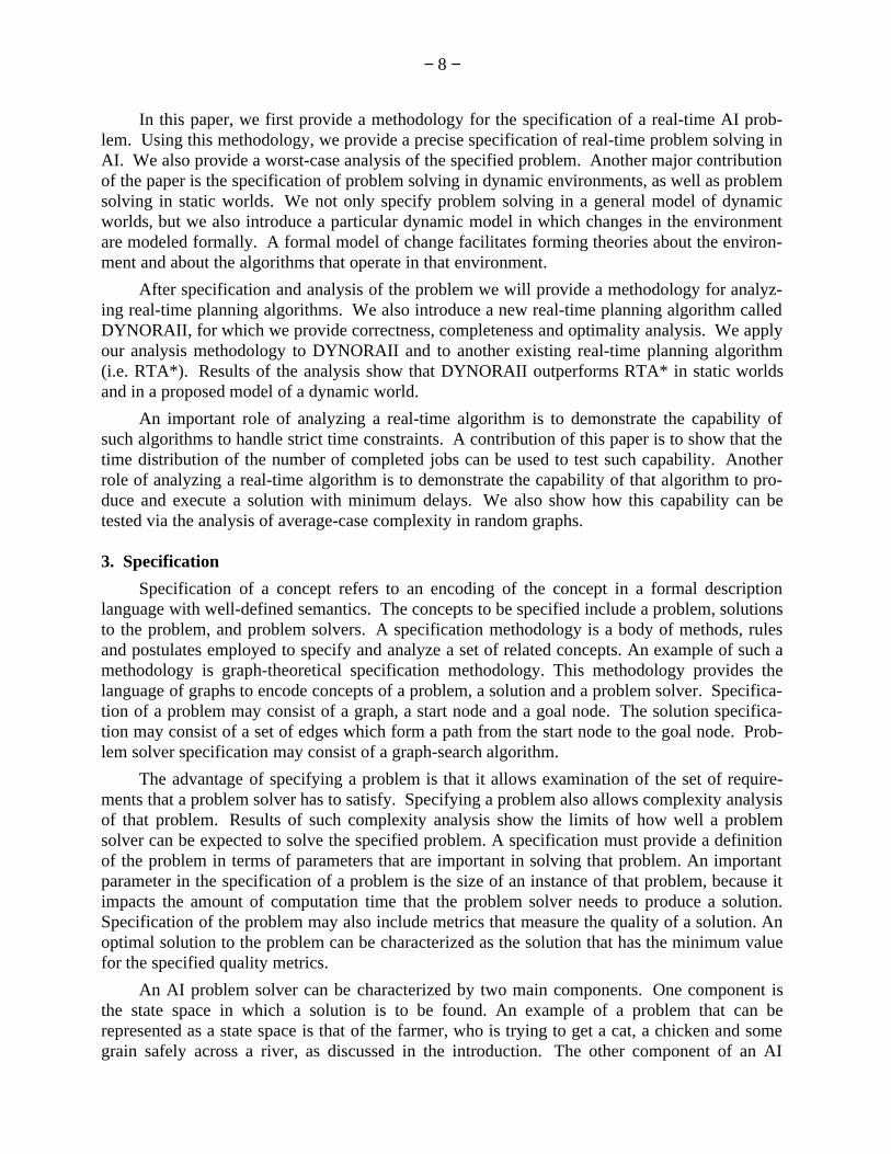
In a dynamic state space, execution costs ceviv j(t) are a function of time to reflect the

changes in the world over time. An edge in this graph may cease to exist for a period of time.This is represented by an execution cost of ∞ associated with that edge for that period of time.Next, we will specify a simple † formal model of change in a dynamic environment. The pro-posed model of change is based on a Markov process. The selected Markov process is used tochange the cost of the edges in the graph to simulate a dynamic world. A cost ceviv j

(t) in thismodel is considered to be a random variable and a function of time. The change of the cost of anedge in time is modeled by a bounded Markov process as follows:

The bounds on the Markov process keep the edge cost distributions from diverging too faraway from the mean. The bounds satisfy the following property: 0 ≤ ceviv j

min < ceviv j

max. Ifceviv j

max=∞, then an existing edge may become virtually non-existent within a finite time, as itscost becomes much larger than the cost of other edges. An optimal solution to the path-planningproblem, in the proposed dynamic world model, is a path with the least average total cost ofplanning and execution at/over some time point or interval. A statistically optimal solution path

† Modeling "real" dynamic problems is outside the scope of this paper.

− 10 −

Figure 2: Dynamic Edge Cost Model at Time t (i.e. ceviv j(t)).

Assume σ<<(ceviv j

max − ceviv j

min.

ranges of ceviv j(t−1) Equally Probable Values of ceviv j

(t)

Value 1, (Pr. = 1/2) Value 2, (Pr. = 1/2)

(ceviv j

max−σ, ceviv j

max] ceviv j(t−1) ceviv j

(t−1)−σ

[ceviv j

min, ceviv j

min+σ) ceviv j(t−1) ceviv j

(t−1)+σ

[ceviv j

min+σ , ceviv j

max−σ] ceviv j(t−1)+σ ceviv j

(t−1)−σ

is the path which is most likely to be the best over any interval of time.

Lastly, we discuss the notion of random graphs to specify the average-case behavior ofreal-time problem solvers. We define a random graph to be a graph G(V, P) in which each edgeexists with a certain probability P. In the case where P=1, the graph is completely connected;namely every node is directly connected to all other nodes with single edges. P=0 signifies agraph with no edges. The choice of P influences the likelihood of the number of solution pathswith certain lengths[37].

The constraints on the total response time of the planning and execution processes of real-time problem solvers can be specified as follows. Total response times are characterized by thesum of the time it takes to plan a solution and the time it takes to execute that solution. If theexecution cost Ce and the planning cost Cp of a solution path in a state space are calculated interms of time, the total response time of a plan can be calculated as Cp + Ce . Strict time con-straints on total response times typically pose deadlines on the amount of time available for plan-ning and execution of a solution. In such situations, a planning algorithm is required to plan apath from the start node to the goal node and to execute that path, namely to traverse all edges inthe path and end up at the goal state before a deadline is reached. Deadline situations requireguarantees on total response times. Other, less strict, time constraints pose optimality conditionson total response times. These situations, while they do not pose hard deadlines, do requireminimum delays in planning and executing a solution. A goal state, in such situations, must bereached in as little amount of time as possible (i.e. the total response time Ce + Cp is a minimum).In analyzing the algorithms addressing the problem of real-time planning and search, we willtake into account the ability of these algorithms to meet deadlines, as well as their ability tominimize total response times.

4. Analysis

The analysis methodology can be divided into two parts. In one part of the methodology,the specified problem is analyzed independently of the algorithm that is intended to solve it.This part of the analysis can consist of analytical results on worst-case time complexity of theproblem. Other analysis can evaluate solution density and solution quality. A solution densityanalysis is concerned with the number of solutions that exist in an average-case or a worst-casestate space. A solution quality analysis is concerned with how good a solution, in terms of someparameter(s) of interest, one can expect from an algorithm. Both of the latter analyses, namelythe solution density and solution quality analysis, can help to determine the worst-case timecomplexity of the specified problem.

− 11 −

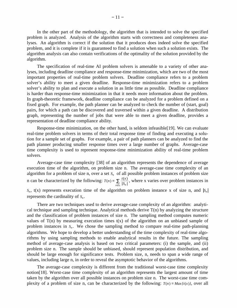
In the other part of the methodology, the algorithm that is intended to solve the specifiedproblem is analyzed. Analysis of the algorithm starts with correctness and completeness ana-lyses. An algorithm is correct if the solution that it produces does indeed solve the specifiedproblem, and it is complete if it is guaranteed to find a solution when such a solution exists. Thealgorithm analysis can also contain verifications of the optimality of the solution provided by thealgorithm.

The specification of real-time AI problem solvers is amenable to a variety of other ana-lyses, including deadline compliance and response-time minimization, which are two of the mostimportant properties of real-time problem solvers. Deadline compliance refers to a problemsolver’s ability to meet a given deadline. Response-time minimization refers to a problemsolver’s ability to plan and execute a solution in as little time as possible. Deadline complianceis harder than response-time minimization in that it needs more information about the problem.In graph-theoretic framework, deadline compliance can be analyzed for a problem defined on afixed graph. For example, the path planner can be analyzed to check the number of (start, goal)pairs, for which a path can be discovered and traversed within a given deadline. A distributiongraph, representing the number of jobs that were able to meet a given deadline, provides arepresentation of deadline compliance ability.

Response-time minimization, on the other hand, is seldom infeasible[19]. We can evaluatereal-time problem solvers in terms of their total response time of finding and executing a solu-tion for a sample set of graphs. For example, a pair of path planners can be analyzed to find thepath planner producing smaller response times over a large number of graphs. Average-casetime complexity is used to represent response-time minimization ability of real-time problemsolvers.

Average-case time complexity [38] of an algorithm represents the dependence of averageexecution time of the algorithm, on problem size n. The average-case time complexity of analgorithm for a problem of size n, over a set Sn of all possible problem instances of problem size

n can be characterized by the following: T(n) =xεSn

Σ |Sn |t(x) , where x varies over problem instances in

Sn, t(x) represents execution time of the algorithm on problem instance x of size n, and |Sn|represents the cardinality of Sn.

There are two techniques used to derive average-case complexity of an algorithm: analyti-cal technique and sampling technique. Analytical methods derive T(n) by analyzing the structureand the classification of problem instances of size n. The sampling method computes numericvalues of T(n) by measuring execution times t(x) of the algorithm on an unbiased sample ofproblem instances in Sn. We chose the sampling method to compare real-time path-planningalgorithms. We hope to develop a better understanding of the time complexity of real-time algo-rithms by using sampling methods to enable analytical results in the future. The samplingmethod of average-case analysis is based on two critical parameters: (i) the sample, and (ii)problem size n. The sample should be unbiased, should represent population distribution, andshould be large enough for significance tests. Problem size, n, needs to span a wide range ofvalues, including large n, in order to reveal the asymptotic behavior of the algorithms.

The average-case complexity is different from the traditional worst-case time complexitynotion[18]. Worst-case time complexity of an algorithm represents the largest amount of timetaken by the algorithm over all possible instances on problem size n. The worst-case time com-plexity of a problem of size n, can be characterized by the following: T(n) = Max{t(x)}, over all

− 12 −

problem instances xεSn of size n, where t(x) is the time complexity of the algorithm on instancex of size n.

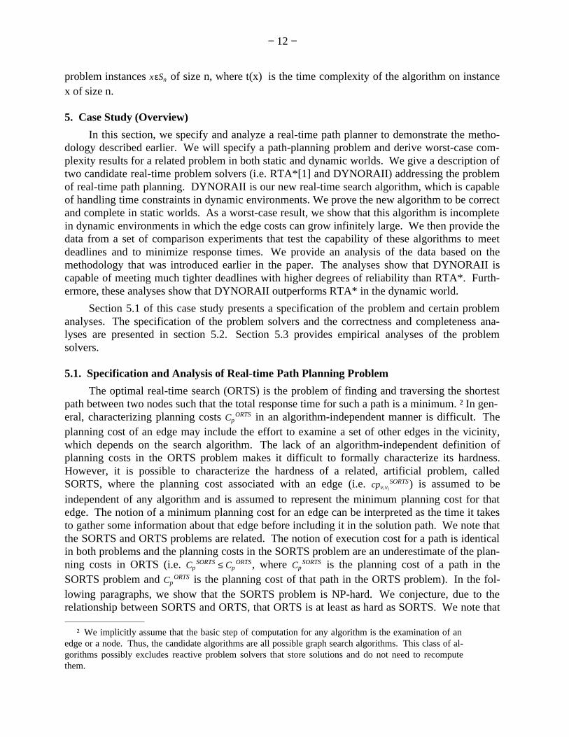
5. Case Study (Overview)

In this section, we specify and analyze a real-time path planner to demonstrate the metho-dology described earlier. We will specify a path-planning problem and derive worst-case com-plexity results for a related problem in both static and dynamic worlds. We give a description oftwo candidate real-time problem solvers (i.e. RTA*[1] and DYNORAII) addressing the problemof real-time path planning. DYNORAII is our new real-time search algorithm, which is capableof handling time constraints in dynamic environments. We prove the new algorithm to be correctand complete in static worlds. As a worst-case result, we show that this algorithm is incompletein dynamic environments in which the edge costs can grow infinitely large. We then provide thedata from a set of comparison experiments that test the capability of these algorithms to meetdeadlines and to minimize response times. We provide an analysis of the data based on themethodology that was introduced earlier in the paper. The analyses show that DYNORAII iscapable of meeting much tighter deadlines with higher degrees of reliability than RTA*. Furth-ermore, these analyses show that DYNORAII outperforms RTA* in the dynamic world.

Section 5.1 of this case study presents a specification of the problem and certain problemanalyses. The specification of the problem solvers and the correctness and completeness ana-lyses are presented in section 5.2. Section 5.3 provides empirical analyses of the problemsolvers.

5.1. Specification and Analysis of Real-time Path Planning Problem

The optimal real-time search (ORTS) is the problem of finding and traversing the shortestpath between two nodes such that the total response time for such a path is a minimum. † In gen-eral, characterizing planning costs Cp

ORTS in an algorithm-independent manner is difficult. Theplanning cost of an edge may include the effort to examine a set of other edges in the vicinity,which depends on the search algorithm. The lack of an algorithm-independent definition ofplanning costs in the ORTS problem makes it difficult to formally characterize its hardness.However, it is possible to characterize the hardness of a related, artificial problem, calledSORTS, where the planning cost associated with an edge (i.e. cpviv j

SORTS) is assumed to beindependent of any algorithm and is assumed to represent the minimum planning cost for thatedge. The notion of a minimum planning cost for an edge can be interpreted as the time it takesto gather some information about that edge before including it in the solution path. We note thatthe SORTS and ORTS problems are related. The notion of execution cost for a path is identicalin both problems and the planning costs in the SORTS problem are an underestimate of the plan-ning costs in ORTS (i.e. Cp

SORTS ≤ CpORTS, where Cp

SORTS is the planning cost of a path in theSORTS problem and Cp

ORTS is the planning cost of that path in the ORTS problem). In the fol-lowing paragraphs, we show that the SORTS problem is NP-hard. We conjecture, due to therelationship between SORTS and ORTS, that ORTS is at least as hard as SORTS. We note that

† We implicitly assume that the basic step of computation for any algorithm is the examination of anedge or a node. Thus, the candidate algorithms are all possible graph search algorithms. This class of al-gorithms possibly excludes reactive problem solvers that store solutions and do not need to recomputethem.

− 13 −

the assumption about the independence of cpviv jfrom the search algorithm is artificial and that

this assumption is not used in designing algorithms proposed in later sections.

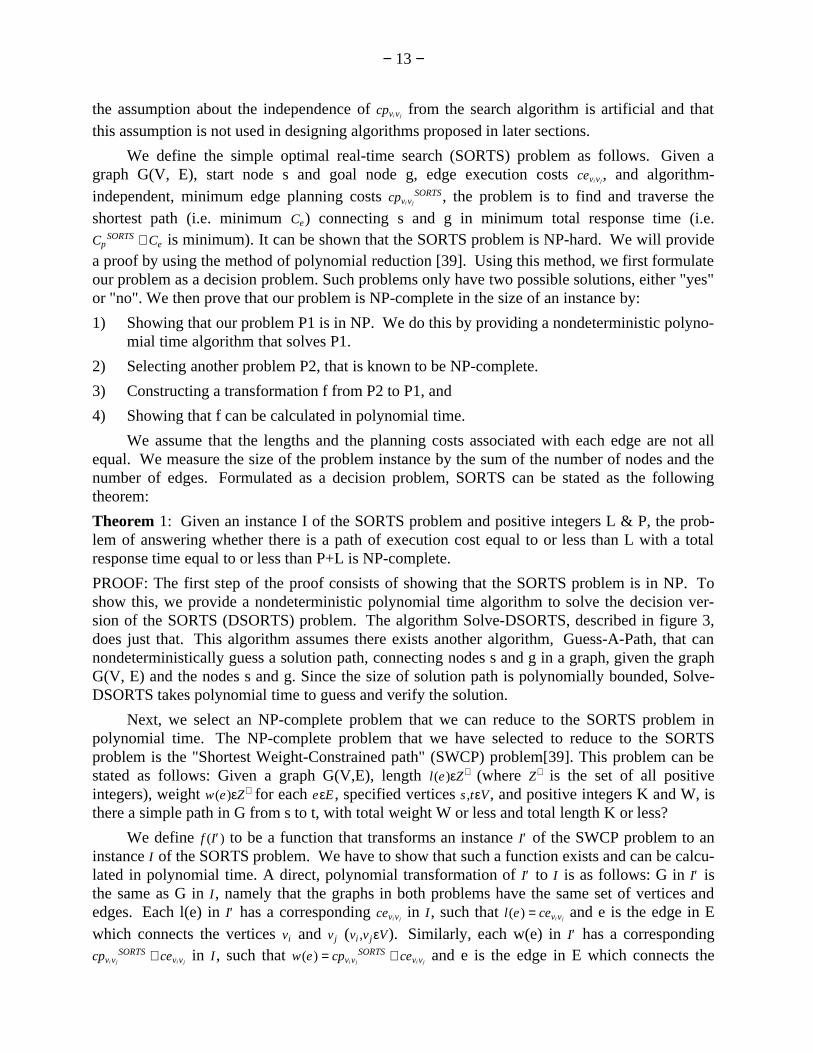
We define the simple optimal real-time search (SORTS) problem as follows. Given agraph G(V, E), start node s and goal node g, edge execution costs ceviv j

, and algorithm-independent, minimum edge planning costs cpviv j

SORTS, the problem is to find and traverse theshortest path (i.e. minimum Ce) connecting s and g in minimum total response time (i.e.Cp

SORTS + Ce is minimum). It can be shown that the SORTS problem is NP-hard. We will providea proof by using the method of polynomial reduction [39]. Using this method, we first formulateour problem as a decision problem. Such problems only have two possible solutions, either "yes"or "no". We then prove that our problem is NP-complete in the size of an instance by:

1) Showing that our problem P1 is in NP. We do this by providing a nondeterministic polyno-mial time algorithm that solves P1.

2) Selecting another problem P2, that is known to be NP-complete.

3) Constructing a transformation f from P2 to P1, and

4) Showing that f can be calculated in polynomial time.

We assume that the lengths and the planning costs associated with each edge are not allequal. We measure the size of the problem instance by the sum of the number of nodes and thenumber of edges. Formulated as a decision problem, SORTS can be stated as the followingtheorem:

Theorem 1: Given an instance I of the SORTS problem and positive integers L & P, the prob-lem of answering whether there is a path of execution cost equal to or less than L with a totalresponse time equal to or less than P+L is NP-complete.

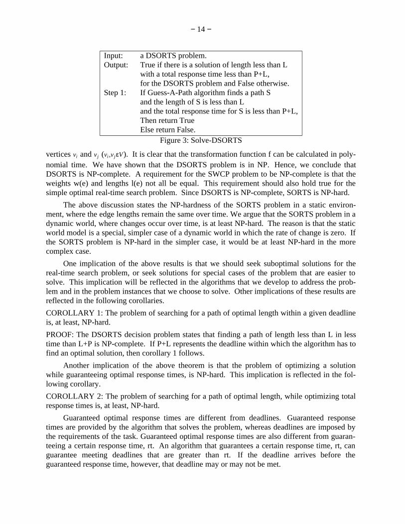
PROOF: The first step of the proof consists of showing that the SORTS problem is in NP. Toshow this, we provide a nondeterministic polynomial time algorithm to solve the decision ver-sion of the SORTS (DSORTS) problem. The algorithm Solve-DSORTS, described in figure 3,does just that. This algorithm assumes there exists another algorithm, Guess-A-Path, that cannondeterministically guess a solution path, connecting nodes s and g in a graph, given the graphG(V, E) and the nodes s and g. Since the size of solution path is polynomially bounded, Solve-DSORTS takes polynomial time to guess and verify the solution.

Next, we select an NP-complete problem that we can reduce to the SORTS problem inpolynomial time. The NP-complete problem that we have selected to reduce to the SORTSproblem is the "Shortest Weight-Constrained path" (SWCP) problem[39]. This problem can bestated as follows: Given a graph G(V,E), length l(e)εZ+ (where Z+ is the set of all positiveintegers), weight w(e)εZ+ for each eεE, specified vertices s ,tεV, and positive integers K and W, isthere a simple path in G from s to t, with total weight W or less and total length K or less?

We define f (I′ ) to be a function that transforms an instance I′ of the SWCP problem to aninstance I of the SORTS problem. We have to show that such a function exists and can be calcu-lated in polynomial time. A direct, polynomial transformation of I′ to I is as follows: G in I′ isthe same as G in I , namely that the graphs in both problems have the same set of vertices andedges. Each l(e) in I′ has a corresponding ceviv j

in I , such that l(e) = ceviv jand e is the edge in E

which connects the vertices vi and v j (vi ,v jεV). Similarly, each w(e) in I′ has a correspondingcpviv j

SORTS + ceviv jin I , such that w(e) = cpviv j

SORTS + ceviv jand e is the edge in E which connects the

− 14 −

Input: a DSORTS problem.Output: True if there is a solution of length less than L

with a total response time less than P+L,for the DSORTS problem and False otherwise.

Step 1: If Guess-A-Path algorithm finds a path Sand the length of S is less than Land the total response time for S is less than P+L,Then return TrueElse return False.

Figure 3: Solve-DSORTS

vertices vi and v j (vi ,v jεV). It is clear that the transformation function f can be calculated in poly-nomial time. We have shown that the DSORTS problem is in NP. Hence, we conclude thatDSORTS is NP-complete. A requirement for the SWCP problem to be NP-complete is that theweights w(e) and lengths l(e) not all be equal. This requirement should also hold true for thesimple optimal real-time search problem. Since DSORTS is NP-complete, SORTS is NP-hard.

The above discussion states the NP-hardness of the SORTS problem in a static environ-ment, where the edge lengths remain the same over time. We argue that the SORTS problem in adynamic world, where changes occur over time, is at least NP-hard. The reason is that the staticworld model is a special, simpler case of a dynamic world in which the rate of change is zero. Ifthe SORTS problem is NP-hard in the simpler case, it would be at least NP-hard in the morecomplex case.

One implication of the above results is that we should seek suboptimal solutions for thereal-time search problem, or seek solutions for special cases of the problem that are easier tosolve. This implication will be reflected in the algorithms that we develop to address the prob-lem and in the problem instances that we choose to solve. Other implications of these results arereflected in the following corollaries.

COROLLARY 1: The problem of searching for a path of optimal length within a given deadlineis, at least, NP-hard.

PROOF: The DSORTS decision problem states that finding a path of length less than L in lesstime than L+P is NP-complete. If P+L represents the deadline within which the algorithm has tofind an optimal solution, then corollary 1 follows.

Another implication of the above theorem is that the problem of optimizing a solutionwhile guaranteeing optimal response times, is NP-hard. This implication is reflected in the fol-lowing corollary.

COROLLARY 2: The problem of searching for a path of optimal length, while optimizing totalresponse times is, at least, NP-hard.

Guaranteed optimal response times are different from deadlines. Guaranteed responsetimes are provided by the algorithm that solves the problem, whereas deadlines are imposed bythe requirements of the task. Guaranteed optimal response times are also different from guaran-teeing a certain response time, rt. An algorithm that guarantees a certain response time, rt, canguarantee meeting deadlines that are greater than rt. If the deadline arrives before theguaranteed response time, however, that deadline may or may not be met.

− 15 −

5.2. Specification of Real-time Path Planners

In this section, we will specify two real-time problem solvers as search algorithms on agraph. The problem solvers are RTA*[1] and DYNORAII [40]. Both of these algorithms workin cycles of partial search followed by execution. The paradigm of partial search followed byexecution helps these algorithms to cope with changes in the environment. Both algorithms usean evaluation function to guide the partial search, like A*[23]. The evaluation function f of anode is calculated as the sum of two parts: g and h (i.e. f = g + h). In A*, g represents the actualcost of a path from the start node to the currently evaluated node in the graph, and h representsthe estimated cost of a path from the current node to the goal node. h is often called a heuristicfunction. It has been shown that A* will find the shortest path in the graph, given a heuristicfunction h that underestimates the cost of a partial path from the current node to the goal node.

RTA* and DYNORAII differ in the stopping criterion used to terminate the partial searchin each cycle and in the way planning time is allocated in each cycle. DYNORAII’s stoppingcriterion enables it to handle time constraints, as well as issues of dynamic worlds. The twoalgorithms also differ in the way they control the search process. RTA* performs a search witha fixed depth bound for each neighbor of the current node. DYNORAII carries out a single A*with a termination criteria based on planning and execution costs. DYNORAII allocates plan-ning effort to the frontier nodes in proportion to their promise, whereas RTA* allocates compar-able planning effort to all neighbors of the current node.

5.2.1. RTA*

At each cycle, RTA*(n) first creates the successor nodes of the current state. The currentstate is the actual position of the system. Parameter n corresponds to the number of descendantnodes evaluated for each neighbor, during a cycle. As each successor node is created, itsestimated distance from the goal (i.e. h), the cost from the current node (i.e. g), and the sum of hand g (i.e. f) are calculated. The euclidean distance formula is used to calculate the h values.This heuristic formula is monotonic [1] and is guaranteed to produce optimal solutions in A*. Inthe case of RTA*, this heuristic formula allows substantial pruning of frontier nodes without lossof valuable information in reaching a partial solution. Notice that, unlike A*, in which g is thevalue of the total cost so far, namely from the start node to the current successor node, in RTA*,g is the value of the cost from the current node to each of its successor nodes. The h values arecalculated via look-ahead search. The algorithm assumes that the larger the number of look-aheads (i.e. the larger the n), the more accurate the estimated f value (i.e. g+h) will be. How-ever, we encountered cases in which the greater look-aheads led the algorithm to more costlysolutions. Also, one must note that while greater look-aheads are generally helpful in findingshorter paths to the goal (i.e. lower execution cost), they require more processing and planning(i.e. higher planning cost). Once all the successor nodes and their f values are determined, thealgorithm sorts these nodes with respect to their f values. The successor node with the smallest fvalue is chosen as the next physical move for the RTA* algorithm. This process is repeated untila solution is reached.

While this algorithm cannot guarantee termination in the case of graphs with no solutions,it does guarantee that it will not get stuck in local minima and graph cycles. This is accom-plished by penalizing cyclic and dead-end paths, and by leaving the h value of the second bestpath at each decision point [1]. This algorithm has been shown to be correct and complete instatic worlds[1].

− 16 −

5.2.2. DYnamic Near Optimal Response-time Algorithm II (DYNORAII)

DYNORAII performs planning and execution cycles repeatedly until a goal node isreached, assuming that the graph has a solution. A plan-execute cycle starts with conducting aheuristic search (plan phase) for the next move, starting at the current state (node) in the graph.The search continues from the start state to a variable depth in the graph until the following stop-ping criterion is met:

Cp ≥ αCe (1)

This stopping criterion provides a tradeoff between the total planning cost (Cp) so far, accumu-lated during the entire planning phase of the current cycle, and the best estimated execution cost(Ce) of a complete path, found during the planning phase of the current cycle. This tradeofftakes into account the utility of the heuristic solution found in the current plan phase versus theamount of planning that was performed to find that solution.

During the execute phase, the algorithm commits to the best action found during the previ-ous plan phase. In the case of path planning for a robot, for example, the execute phase consistsof physically moving the robot from its current position to its next position, which was chosenfrom among a set of available options. Figure 4. provides pseudo-code of the DYNORAII algo-rithm.

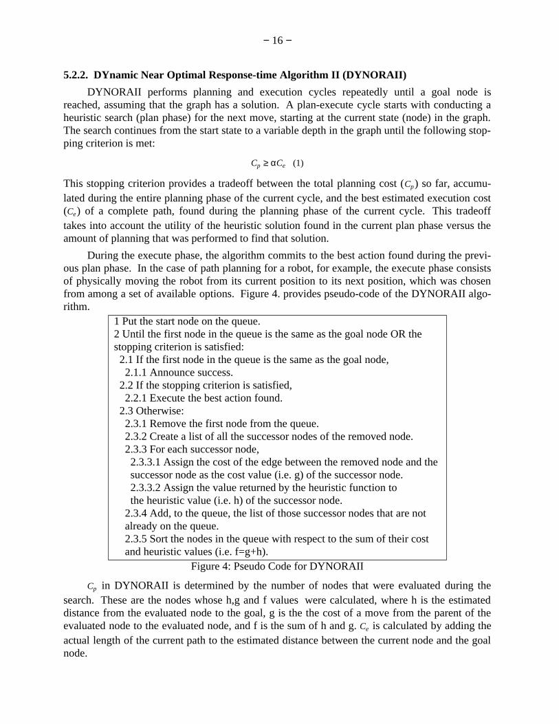
1 Put the start node on the queue.2 Until the first node in the queue is the same as the goal node OR thestopping criterion is satisfied:2.1 If the first node in the queue is the same as the goal node,2.1.1 Announce success.

2.2 If the stopping criterion is satisfied,2.2.1 Execute the best action found.

2.3 Otherwise:2.3.1 Remove the first node from the queue.2.3.2 Create a list of all the successor nodes of the removed node.2.3.3 For each successor node,2.3.3.1 Assign the cost of the edge between the removed node and thesuccessor node as the cost value (i.e. g) of the successor node.2.3.3.2 Assign the value returned by the heuristic function tothe heuristic value (i.e. h) of the successor node.

2.3.4 Add, to the queue, the list of those successor nodes that are notalready on the queue.2.3.5 Sort the nodes in the queue with respect to the sum of their costand heuristic values (i.e. f=g+h).

Figure 4: Pseudo Code for DYNORAII

Cp in DYNORAII is determined by the number of nodes that were evaluated during thesearch. These are the nodes whose h,g and f values were calculated, where h is the estimateddistance from the evaluated node to the goal, g is the the cost of a move from the parent of theevaluated node to the evaluated node, and f is the sum of h and g. Ce is calculated by adding theactual length of the current path to the estimated distance between the current node and the goalnode.

− 17 −

To explain the advantage of the tradeoff between planning cost and execution cost, con-sider RTA* as an example of a real-time search algorithm. RTA* [1] uses a fixed look-ahead,specifying a static bound for the look-ahead search. When this look-ahead bound is reached,RTA* stops the look-ahead search regardless of the quality of the solution found and regardlessof the amount of search done. In some cases, the search terminates prematurely, resulting in apoor (i.e. costly) solution. In some other cases, too much searching is done for little gain in solu-tion quality. In DYNORAII the search bound is reached when a balance between planning costand execution cost is reached (i.e. the stopping criterion of inequality 1 is met). Hence, thedepth of search in this algorithm is determined dynamically.

When the criterion of inequality 1 is satisfied, the smallest f value found so far is returnedto the top level of the algorithm. The successor node with the smallest f value is chosen as thenext physical move for the DYNORAII algorithm. This process is repeated until a solution isreached.

An important parameter involved in the tradeoff between Cp and Ce is α (see inequality 1).The appropriate value of α depends on certain characteristics of the graph and of the applicationat hand. Examples of such characteristics are the graph size, the branching factor, and the timeavailable for planning. The general rule of thumb is to choose a large α when the search space issmall, the branching factor is small and the time to plan is long. A small α is chosen when thesearch space is large, the branching factor is large and the time to plan is short. The intuitiverationale behind these heuristics is that a large graph or a high branching factor with a large αcan considerably increase the amount of planning. Also, when the available time to plan isshort, one must obviously reduce the amount of planning in each plan-execute cycle.

DYNORAII guarantees termination if a solution path from start node to goal node exists ina finite graph with bidirectional edges. It also is able to get out of local minima and graphcycles. This is accomplished by penalizing cyclic and dead-end paths, and by leaving the hvalue of the second-best path at each decision point [1]. Next, we will present some formalresults regarding the algorithm and its performance. Empirical results based on performancecomparison experiments will follow.

Theorem 2: If DYNORAII, given a problem, terminates claiming a solution, the answer it pro-duces does in fact solve the given problem.

PROOF: A solution is correct when it connects the start state to the goal state via legal moves.DYNORAII always starts its plan-execute cycles from the initial state. It then executes its par-tial plans until success in finding a solution is announced. Thus, if DYNORAII announces suc-cess when it has reached the goal state, it has found the correct solution. It is indeed the casethat DYNORAII announces success only when it has executed a move that has led to the goalstate. Therefore, DYNORAII’s solution does solve a given problem.

By proving the next theorem, we will show that under a set of assumptions DYNORAII isguaranteed to produce a response (i.e. find a goal state) if such a solution exists. We will showour results for the general case of graphs that may include cycles. We will assume a finitesearch space. In an infinite space, deceiving heuristic values may send DYNORAII down aninfinite path which never reaches a solution. We assume positive edge costs that remain constantover time. In proving the next theorem, we will relax this assumption to explore completenessof DYNORAII in dynamic worlds. Finally, we assume bidirectional edges to allow our algo-rithm to backtrack out of dead-end paths.

− 18 −

Theorem 3: In a finite problem space with bidirectional edges, static positive edge costs andfinite heuristic values, where there exists a path that connects the start node to the goal node,DYNORAII is guaranteed to find that path.

PROOF: We will prove this theorem by contradiction. Assume that the negation of the theoremis true, namely that there may be a path from the start node to the goal node in the search space,and that DYNORAII never reaches that path. For such a situation to be true, there must exist acycle in the graph that does not include the goal node, in which the algorithm loops infinitely.On the other hand, it is true that if a path exists from start to goal, the goal node is reachablefrom every node in the component of the graph in which the start and goal nodes reside. Thus,there must exist an edge that leads away from the cycle and that connects to the goal node. Wenow have to show that DYNORAII will ultimately leave this cycle. Associated with every nodein the graph is a heuristic value which is either calculated (if the node has not been visitedbefore) or is retrieved (if the node has been visited before and thus has inherited the second bestf value of its children). In moving from a node x to a child node C1, DYNORAII calculates orretrieves the fci

values of its children, adds the corresponding positive edge costs (gx(ci)), andmoves to the child (C1 in this case) with the lowest resulting value. It also assigns the secondbest fci

value as the heuristic value of the node x (i.e.h(x)←fciwhere fci

is the second best f valueof x’s children). Since the second best value is greater than or equal to the best value, and thevalue of the new state, C1, is strictly less than its value after the cost of the edge from the oldstate x is added to it(due to positive edge costs), the value of the node x must be strictly greaterthan the value of node C1. Thus, the value of the old state is always larger than the value of thenew state. Now consider the node with the smallest value on the cycle as the current state.Upon leaving this state, a new, larger value is assigned to this node. Furthermore, upon reachingthis node for the second time, its value is increased again due to the reasoning given above. Ifthis is true for the node with smallest value, then it is true for all nodes on the cycle. In the caseof static edge costs, the values of all nodes on the cycle increase monotonically without bounds.The time will finally come when the value of the node on the path away from this cycle is lowerthan the value of its neighbor on the cycle. At that time, DYNORAII will get out of the cycle.This is in contradiction with our assumption of an infinite loop. We conclude that under theassumptions of our theorem, there do not exist any infinite loops. This proves our theorem forthe static case.

The next theorem addresses completeness of DYNORAII in dynamic worlds. Here weshow, via an example, that in dynamic environments, in general, where the costs of moves cangrow infinitely large, DYNORAII is not a complete algorithm. This implies that DYNORAIIcan oscillate between a set of nodes or fall into an infinite loop and never find a solution, even ifsuch a solution exists.

Theorem 4: DYNORAII is not complete in a dynamic environment in which the edge costs arepositive and can grow infinitely large.

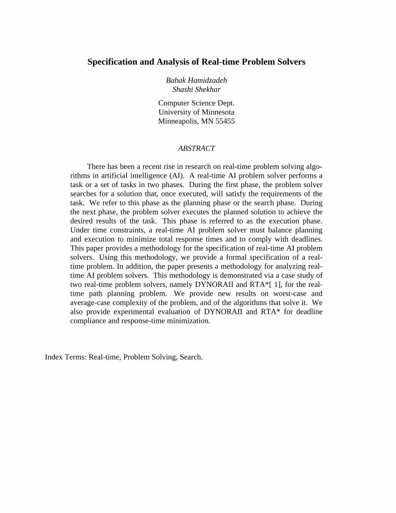
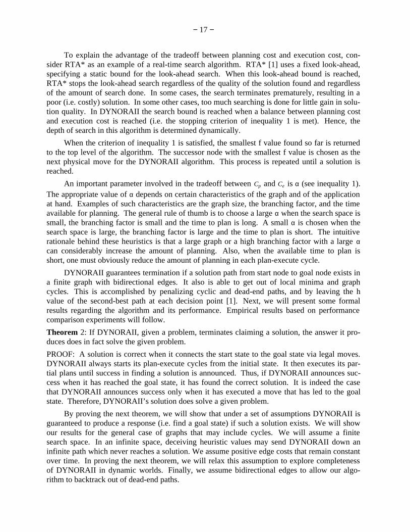
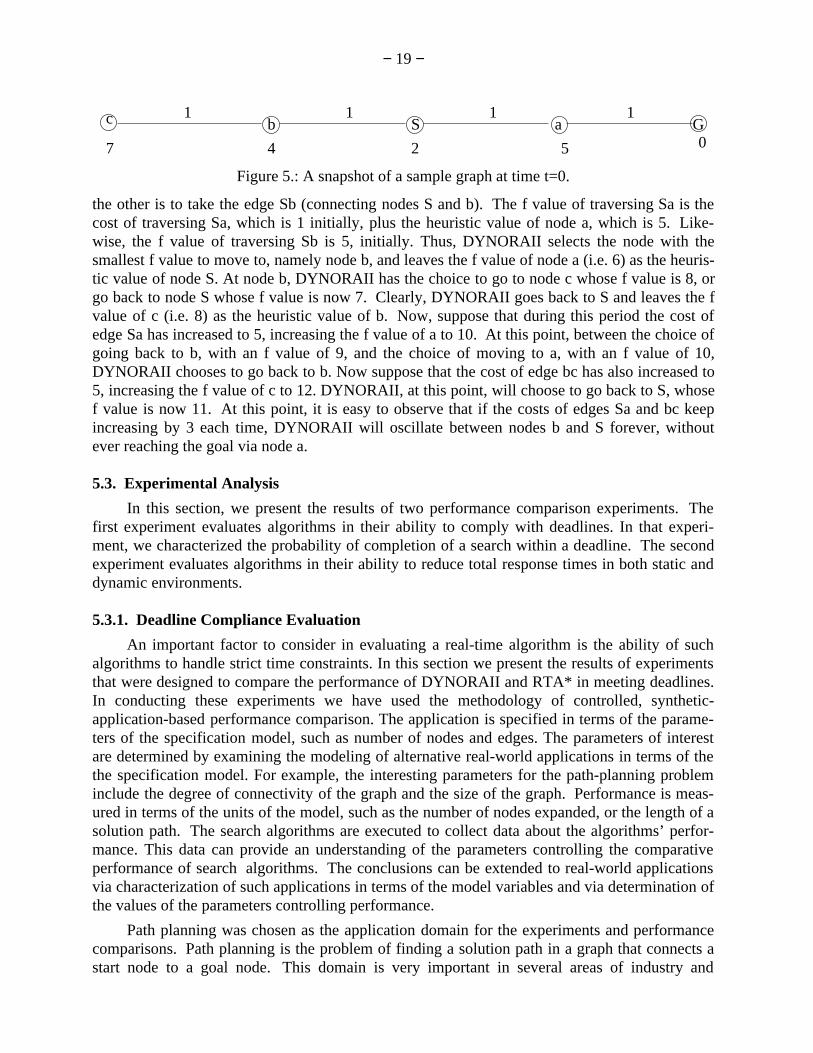
PROOF: Consider the following example of a graph with dynamic edge costs, depicted in figure5.

The edge costs are all set at 1, initially. The heuristic value of each node is written in theboxes below each node. Assume that the node S is the starting position and that we want to plana path to node G. Also, assume that DYNORAII’s look-ahead is set so that the algorithm canonly look at the immediate successors of a node when the algorithm is in its planning phase.From node S, we have two choices. One is to take the edge Sa (connecting nodes S and a), and

− 19 −

7 4 052

1111c b a GS

Figure 5.: A snapshot of a sample graph at time t=0.

the other is to take the edge Sb (connecting nodes S and b). The f value of traversing Sa is thecost of traversing Sa, which is 1 initially, plus the heuristic value of node a, which is 5. Like-wise, the f value of traversing Sb is 5, initially. Thus, DYNORAII selects the node with thesmallest f value to move to, namely node b, and leaves the f value of node a (i.e. 6) as the heuris-tic value of node S. At node b, DYNORAII has the choice to go to node c whose f value is 8, orgo back to node S whose f value is now 7. Clearly, DYNORAII goes back to S and leaves the fvalue of c (i.e. 8) as the heuristic value of b. Now, suppose that during this period the cost ofedge Sa has increased to 5, increasing the f value of a to 10. At this point, between the choice ofgoing back to b, with an f value of 9, and the choice of moving to a, with an f value of 10,DYNORAII chooses to go back to b. Now suppose that the cost of edge bc has also increased to5, increasing the f value of c to 12. DYNORAII, at this point, will choose to go back to S, whosef value is now 11. At this point, it is easy to observe that if the costs of edges Sa and bc keepincreasing by 3 each time, DYNORAII will oscillate between nodes b and S forever, withoutever reaching the goal via node a.

5.3. Experimental Analysis

In this section, we present the results of two performance comparison experiments. Thefirst experiment evaluates algorithms in their ability to comply with deadlines. In that experi-ment, we characterized the probability of completion of a search within a deadline. The secondexperiment evaluates algorithms in their ability to reduce total response times in both static anddynamic environments.

5.3.1. Deadline Compliance Evaluation

An important factor to consider in evaluating a real-time algorithm is the ability of suchalgorithms to handle strict time constraints. In this section we present the results of experimentsthat were designed to compare the performance of DYNORAII and RTA* in meeting deadlines.In conducting these experiments we have used the methodology of controlled, synthetic-application-based performance comparison. The application is specified in terms of the parame-ters of the specification model, such as number of nodes and edges. The parameters of interestare determined by examining the modeling of alternative real-world applications in terms of thethe specification model. For example, the interesting parameters for the path-planning probleminclude the degree of connectivity of the graph and the size of the graph. Performance is meas-ured in terms of the units of the model, such as the number of nodes expanded, or the length of asolution path. The search algorithms are executed to collect data about the algorithms’ perfor-mance. This data can provide an understanding of the parameters controlling the comparativeperformance of search algorithms. The conclusions can be extended to real-world applicationsvia characterization of such applications in terms of the model variables and via determination ofthe values of the parameters controlling performance.

Path planning was chosen as the application domain for the experiments and performancecomparisons. Path planning is the problem of finding a solution path in a graph that connects astart node to a goal node. This domain is very important in several areas of industry and

− 20 −

%

Jobs

Completed

(Time-Units)

DYNORAII(0.1)

DYNORAII(1)

DYNORAII (0.05)

DYNORAII (0.5)

0 100 200 300 400 500 600 700 800 900 1000

20

40

60

80

100

Deadline

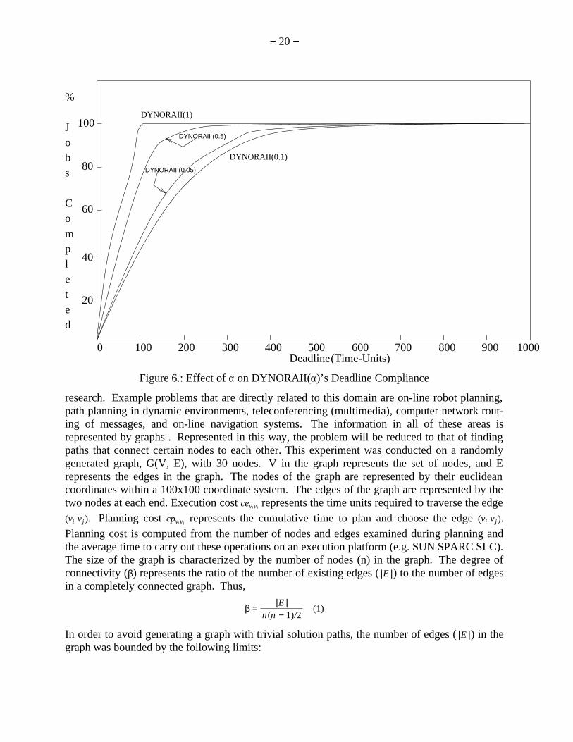
Figure 6.: Effect of α on DYNORAII(α)’s Deadline Compliance

research. Example problems that are directly related to this domain are on-line robot planning,path planning in dynamic environments, teleconferencing (multimedia), computer network rout-ing of messages, and on-line navigation systems. The information in all of these areas isrepresented by graphs . Represented in this way, the problem will be reduced to that of findingpaths that connect certain nodes to each other. This experiment was conducted on a randomlygenerated graph, G(V, E), with 30 nodes. V in the graph represents the set of nodes, and Erepresents the edges in the graph. The nodes of the graph are represented by their euclideancoordinates within a 100x100 coordinate system. The edges of the graph are represented by thetwo nodes at each end. Execution cost ceviv j

represents the time units required to traverse the edge(vi v j). Planning cost cpviv j

represents the cumulative time to plan and choose the edge (vi v j).Planning cost is computed from the number of nodes and edges examined during planning andthe average time to carry out these operations on an execution platform (e.g. SUN SPARC SLC).The size of the graph is characterized by the number of nodes (n) in the graph. The degree ofconnectivity (β) represents the ratio of the number of existing edges ( |E |) to the number of edgesin a completely connected graph. Thus,

β =n(n − 1)/2

|E |(1)

In order to avoid generating a graph with trivial solution paths, the number of edges ( |E |) in thegraph was bounded by the following limits:

− 21 −

Number

of

Samples

(Time-Units)0 100 200 300 400 500 600 700 800 900 1000

20

40

60

80

100

120

140

DYNORAII(0.05)

DYNORAII(0.5)

DYNORAII(1)

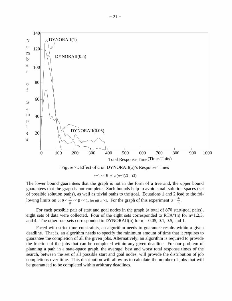
Total Response Time

Figure 7.: Effect of α on DYNORAII(α)’s Response Times

n−1 << E << n(n−1)/2 (2)

The lower bound guarantees that the graph is not in the form of a tree and, the upper boundguarantees that the graph is not complete. Such bounds help to avoid small solution spaces (setof possible solution paths), as well as trivial paths to the goal. Equations 1 and 2 lead to the fol-lowing limits on β: 0 <

n2

<< β << 1, for all n>1. For the graph of this experiment β =n4 .

For each possible pair of start and goal nodes in the graph (a total of 870 start-goal pairs),eight sets of data were collected. Four of the eight sets corresponded to RTA*(n) for n=1,2,3,and 4. The other four sets corresponded to DYNORAII(α) for α = 0.05, 0.1, 0.5, and 1.

Faced with strict time constraints, an algorithm needs to guarantee results within a givendeadline. That is, an algorithm needs to specify the minimum amount of time that it requires toguarantee the completion of all the given jobs. Alternatively, an algorithm is required to providethe fraction of the jobs that can be completed within any given deadline. For our problem ofplanning a path in a state-space graph, the average, best and worst total response times of thesearch, between the set of all possible start and goal nodes, will provide the distribution of jobcompletions over time. This distribution will allow us to calculate the number of jobs that willbe guaranteed to be completed within arbitrary deadlines.

− 22 −

%

Jobs

Completed

(Time-Units)Deadline

RTA*(4)

RTA*(3)RTA*(2)

RTA*(1)100

80

60

40

20

10009008007006005004003002001000

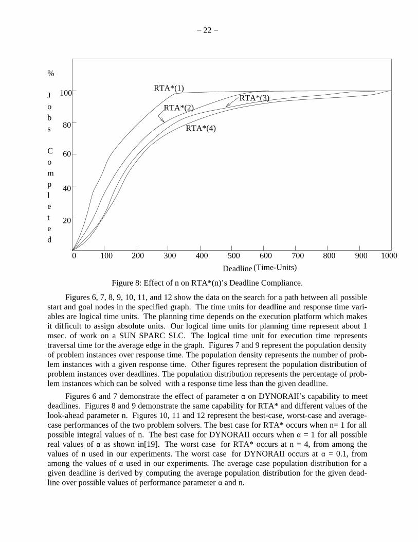
Figure 8: Effect of n on RTA*(n)’s Deadline Compliance.

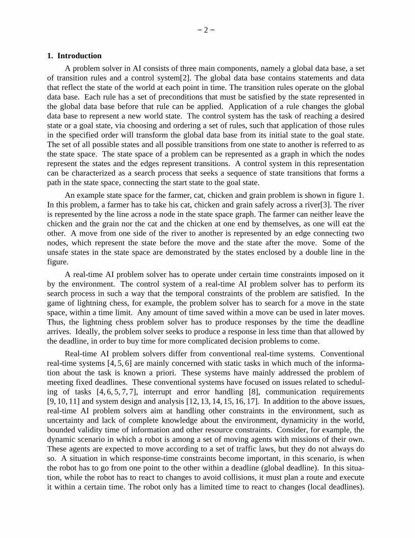
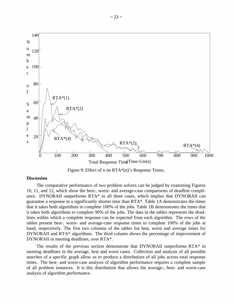
Figures 6, 7, 8, 9, 10, 11, and 12 show the data on the search for a path between all possiblestart and goal nodes in the specified graph. The time units for deadline and response time vari-ables are logical time units. The planning time depends on the execution platform which makesit difficult to assign absolute units. Our logical time units for planning time represent about 1msec. of work on a SUN SPARC SLC. The logical time unit for execution time representstraversal time for the average edge in the graph. Figures 7 and 9 represent the population densityof problem instances over response time. The population density represents the number of prob-lem instances with a given response time. Other figures represent the population distribution ofproblem instances over deadlines. The population distribution represents the percentage of prob-lem instances which can be solved with a response time less than the given deadline.

Figures 6 and 7 demonstrate the effect of parameter α on DYNORAII’s capability to meetdeadlines. Figures 8 and 9 demonstrate the same capability for RTA* and different values of thelook-ahead parameter n. Figures 10, 11 and 12 represent the best-case, worst-case and average-case performances of the two problem solvers. The best case for RTA* occurs when n= 1 for allpossible integral values of n. The best case for DYNORAII occurs when α = 1 for all possiblereal values of α as shown in[19]. The worst case for RTA* occurs at n = 4, from among thevalues of n used in our experiments. The worst case for DYNORAII occurs at α = 0.1, fromamong the values of α used in our experiments. The average case population distribution for agiven deadline is derived by computing the average population distribution for the given dead-line over possible values of performance parameter α and n.

− 23 −

Number

of

Samples

(Time-Units)

RTA*(2) RTA*(4)

0 100 200 300 400 500 600 700 800 900 1000

20

40

60

80

100

120

140

RTA*(1)

RTA*(2)

RTA*(4)

Total Response Time

Figure 9: Effect of n on RTA*(n)’s Response Times.

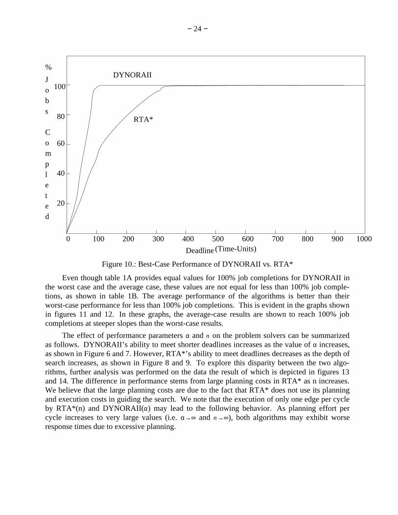
Discussion

The comparative performance of two problem solvers can be judged by examining Figures10, 11, and 12, which show the best-, worst- and average-case comparisons of deadline compli-ance. DYNORAII outperforms RTA* in all three cases, which implies that DYNORAII canguarantee a response in a significantly shorter time than RTA*. Table 1A demonstrates the timesthat it takes both algorithms to complete 100% of the jobs. Table 1B demonstrates the times thatit takes both algorithms to complete 90% of the jobs. The data in the tables represents the dead-lines within which a complete response can be expected from each algorithm. The rows of thetables present best-, worst- and average-case response times to complete 100% of the jobs athand, respectively. The first two columns of the tables list best, worst and average times forDYNORAII and RTA* algorithms. The third column shows the percentage of improvement ofDYNORAII in meeting deadlines, over RTA*.

The results of the previous section demonstrate that DYNORAII outperforms RTA* inmeeting deadlines in the average, best and worst cases. Collection and analysis of all possiblesearches of a specific graph allow us to produce a distribution of all jobs across total responsetimes. The best- and worst-case analysis of algorithm performance requires a complete sampleof all problem instances. It is this distribution that allows the average-, best- and worst-caseanalysis of algorithm performance.

− 24 −

%

Jobs

Completed

(Time-Units)

20

40

60

80

100

Deadline

RTA*

DYNORAII

10009008007006005004003002001000

Figure 10.: Best-Case Performance of DYNORAII vs. RTA*

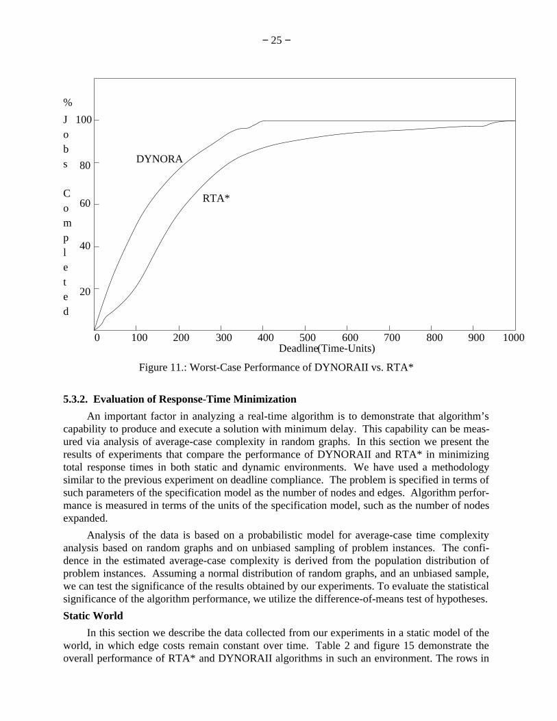
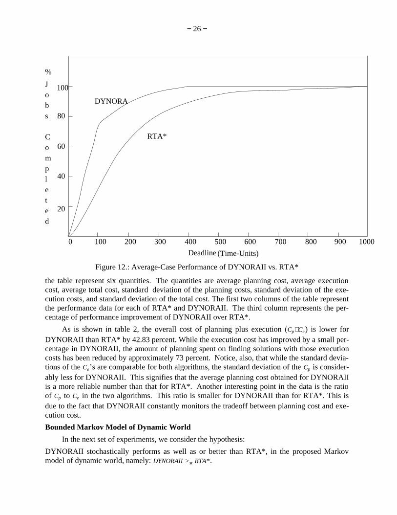
Even though table 1A provides equal values for 100% job completions for DYNORAII inthe worst case and the average case, these values are not equal for less than 100% job comple-tions, as shown in table 1B. The average performance of the algorithms is better than theirworst-case performance for less than 100% job completions. This is evident in the graphs shownin figures 11 and 12. In these graphs, the average-case results are shown to reach 100% jobcompletions at steeper slopes than the worst-case results.

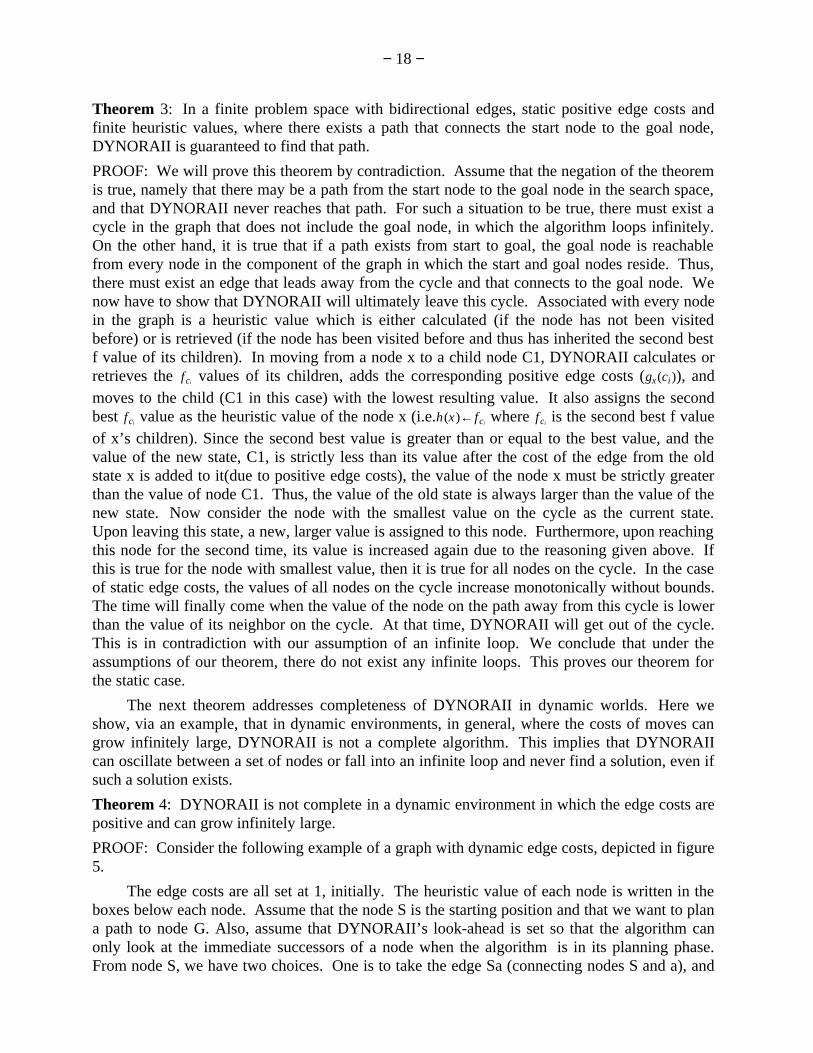
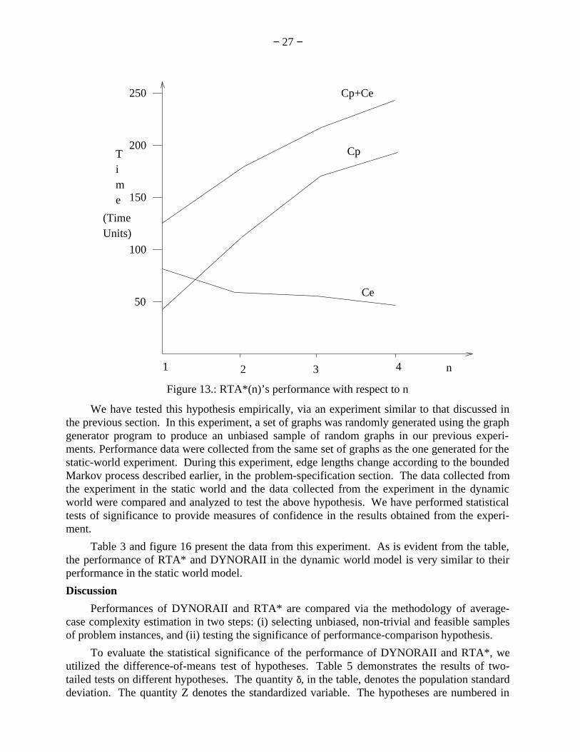
The effect of performance parameters α and n on the problem solvers can be summarizedas follows. DYNORAII’s ability to meet shorter deadlines increases as the value of α increases,as shown in Figure 6 and 7. However, RTA*’s ability to meet deadlines decreases as the depth ofsearch increases, as shown in Figure 8 and 9. To explore this disparity between the two algo-rithms, further analysis was performed on the data the result of which is depicted in figures 13and 14. The difference in performance stems from large planning costs in RTA* as n increases.We believe that the large planning costs are due to the fact that RTA* does not use its planningand execution costs in guiding the search. We note that the execution of only one edge per cycleby RTA*(n) and DYNORAII(α) may lead to the following behavior. As planning effort percycle increases to very large values (i.e. α→∞ and n→∞), both algorithms may exhibit worseresponse times due to excessive planning.

− 25 −

%

Jobs

Completed

(Time-Units)0 100 200 300 400 500 600 700 800 900 1000

20

40

60

80

100

DYNORA

RTA*

Deadline

Figure 11.: Worst-Case Performance of DYNORAII vs. RTA*

5.3.2. Evaluation of Response-Time Minimization

An important factor in analyzing a real-time algorithm is to demonstrate that algorithm’scapability to produce and execute a solution with minimum delay. This capability can be meas-ured via analysis of average-case complexity in random graphs. In this section we present theresults of experiments that compare the performance of DYNORAII and RTA* in minimizingtotal response times in both static and dynamic environments. We have used a methodologysimilar to the previous experiment on deadline compliance. The problem is specified in terms ofsuch parameters of the specification model as the number of nodes and edges. Algorithm perfor-mance is measured in terms of the units of the specification model, such as the number of nodesexpanded.

Analysis of the data is based on a probabilistic model for average-case time complexityanalysis based on random graphs and on unbiased sampling of problem instances. The confi-dence in the estimated average-case complexity is derived from the population distribution ofproblem instances. Assuming a normal distribution of random graphs, and an unbiased sample,we can test the significance of the results obtained by our experiments. To evaluate the statisticalsignificance of the algorithm performance, we utilize the difference-of-means test of hypotheses.

Static World

In this section we describe the data collected from our experiments in a static model of theworld, in which edge costs remain constant over time. Table 2 and figure 15 demonstrate theoverall performance of RTA* and DYNORAII algorithms in such an environment. The rows in

− 26 −

%

Jobs

Completed

(Time-Units)

100

0 100 200 300 400 500 600 700 800 900 1000

20

40

60

80

DYNORA

RTA*

Deadline

Figure 12.: Average-Case Performance of DYNORAII vs. RTA*

the table represent six quantities. The quantities are average planning cost, average executioncost, average total cost, standard deviation of the planning costs, standard deviation of the exe-cution costs, and standard deviation of the total cost. The first two columns of the table representthe performance data for each of RTA* and DYNORAII. The third column represents the per-centage of performance improvement of DYNORAII over RTA*.

As is shown in table 2, the overall cost of planning plus execution (Cp+Ce) is lower forDYNORAII than RTA* by 42.83 percent. While the execution cost has improved by a small per-centage in DYNORAII, the amount of planning spent on finding solutions with those executioncosts has been reduced by approximately 73 percent. Notice, also, that while the standard devia-tions of the Ce’s are comparable for both algorithms, the standard deviation of the Cp is consider-ably less for DYNORAII. This signifies that the average planning cost obtained for DYNORAIIis a more reliable number than that for RTA*. Another interesting point in the data is the ratioof Cp to Ce in the two algorithms. This ratio is smaller for DYNORAII than for RTA*. This isdue to the fact that DYNORAII constantly monitors the tradeoff between planning cost and exe-cution cost.

Bounded Markov Model of Dynamic World

In the next set of experiments, we consider the hypothesis:

DYNORAII stochastically performs as well as or better than RTA*, in the proposed Markovmodel of dynamic world, namely: DYNORAII >st RTA*.

− 27 −

Units)(Time

Time

3 421

Cp+Ce

Cp

Ce

250

200

150

100

50

n

Figure 13.: RTA*(n)’s performance with respect to n

We have tested this hypothesis empirically, via an experiment similar to that discussed inthe previous section. In this experiment, a set of graphs was randomly generated using the graphgenerator program to produce an unbiased sample of random graphs in our previous experi-ments. Performance data were collected from the same set of graphs as the one generated for thestatic-world experiment. During this experiment, edge lengths change according to the boundedMarkov process described earlier, in the problem-specification section. The data collected fromthe experiment in the static world and the data collected from the experiment in the dynamicworld were compared and analyzed to test the above hypothesis. We have performed statisticaltests of significance to provide measures of confidence in the results obtained from the experi-ment.

Table 3 and figure 16 present the data from this experiment. As is evident from the table,the performance of RTA* and DYNORAII in the dynamic world model is very similar to theirperformance in the static world model.

Discussion

Performances of DYNORAII and RTA* are compared via the methodology of average-case complexity estimation in two steps: (i) selecting unbiased, non-trivial and feasible samplesof problem instances, and (ii) testing the significance of performance-comparison hypothesis.

To evaluate the statistical significance of the performance of DYNORAII and RTA*, weutilized the difference-of-means test of hypotheses. Table 5 demonstrates the results of two-tailed tests on different hypotheses. The quantity δ, in the table, denotes the population standarddeviation. The quantity Z denotes the standardized variable. The hypotheses are numbered in

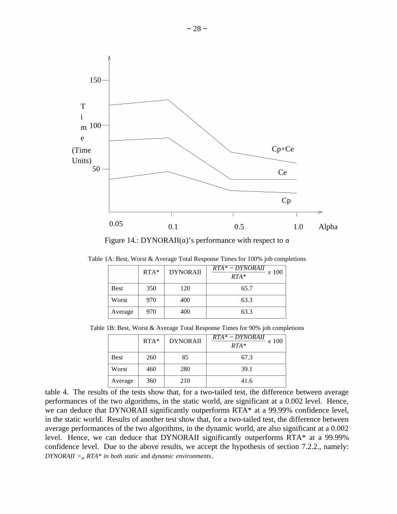
− 28 −

Units)(Time

emiT

Cp+Ce

Cp

Ce

150

100

50

0.05 0.1 0.5 1.0 Alpha

Figure 14.: DYNORAII(α)’s performance with respect to α

Table 1A: Best, Worst & Average Total Response Times for 100% job completions

RTA* DYNORAIIRTA*

RTA* − DYNORAIIx 100

Best 350 120 65.7

Worst 970 400 63.3

Average 970 400 63.3

Table 1B: Best, Worst & Average Total Response Times for 90% job completions

RTA* DYNORAIIRTA*

RTA* − DYNORAIIx 100

Best 260 85 67.3

Worst 460 280 39.1

Average 360 210 41.6

table 4. The results of the tests show that, for a two-tailed test, the difference between averageperformances of the two algorithms, in the static world, are significant at a 0.002 level. Hence,we can deduce that DYNORAII significantly outperforms RTA* at a 99.99% confidence level,in the static world. Results of another test show that, for a two-tailed test, the difference betweenaverage performances of the two algorithms, in the dynamic world, are also significant at a 0.002level. Hence, we can deduce that DYNORAII significantly outperforms RTA* at a 99.99%confidence level. Due to the above results, we accept the hypothesis of section 7.2.2., namely:DYNORAII >st RTA* in both static and dynamic environments .

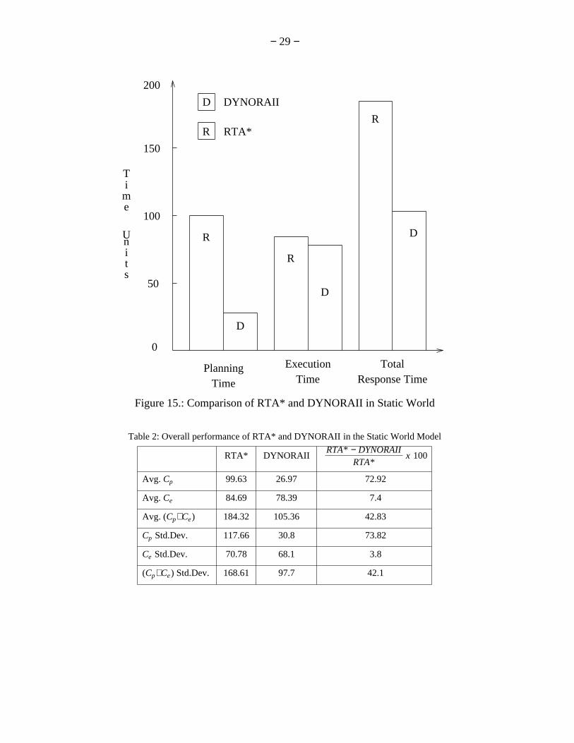
− 29 −

T

U

ime

nits

200

150

100

50

0

D

R RTA*

DYNORAII

R

R

R

D

D

D

PlanningTime

ExecutionTime

TotalResponse Time

Figure 15.: Comparison of RTA* and DYNORAII in Static World

Table 2: Overall performance of RTA* and DYNORAII in the Static World Model

RTA* DYNORAIIRTA*

RTA* − DYNORAIIx 100

Avg. Cp 99.63 26.97 72.92

Avg. Ce 84.69 78.39 7.4

Avg. (Cp+Ce) 184.32 105.36 42.83

Cp Std.Dev. 117.66 30.8 73.82

Ce Std.Dev. 70.78 68.1 3.8

(Cp+Ce) Std.Dev. 168.61 97.7 42.1

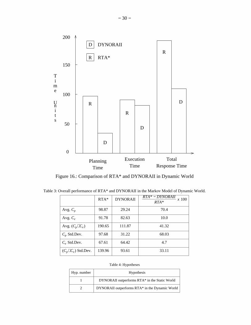
− 30 −

T

U

ime

nits

200

150

100

50

0

D

R RTA*

DYNORAII

R

R

R

D

D

D

PlanningTime

ExecutionTime

TotalResponse Time

Figure 16.: Comparison of RTA* and DYNORAII in Dynamic World

Table 3: Overall performance of RTA* and DYNORAII in the Markov Model of Dynamic World.

RTA* DYNORAIIRTA*

RTA* − DYNORAIIx 100

Avg. Cp 98.87 29.24 70.4

Avg. Ce 91.78 82.63 10.0

Avg. (Cp+Ce) 190.65 111.87 41.32

Cp Std.Dev. 97.68 31.22 68.03

Ce Std.Dev. 67.61 64.42 4.7

(Cp+Ce) Std.Dev. 139.96 93.61 33.11

Table 4: Hypotheses

Hyp. number Hypothesis

1 DYNORAII outperforms RTA* in the Static World

2 DYNORAII outperforms RTA* in the Dynamic World

− 31 −

Table 5: Results of Tests of Hypotheses

Hyp. Number δ Z Test Significance Level Confidence Level

1 12.58 6.28 two-tailed 0.002 99.99

2 10.87 7.25 two-tailed 0.002 99.99

6. Conclusion

Real-time problem solvers in AI can benefit from specification and analysis models basedon graphs. We have presented a specification of real-time path planning problem and the real-time problem solvers for path planning. We have shown that real-time path planning is a hardproblem in order to justify the heuristic approach taken by real-time AI researchers to this prob-lem. We have provided a new heuristic real-time path planning algorithm, DYNORAII. Weexperimentally show that the proposed algorithm outperforms traditional real-time AI algorithmsin deadline compliance and in response-time minimization. We plan to extend the specificationand analysis model to larger problems such as real-time planning and to larger applications suchas robot path planning. We would like to develop benchmarks based on these applications (e.g.lightning chess, tetris, robot path planning) to compare algorithms in a more informative way.We also plan to extend DYNORAII by making parameter α of stopping criterion 1 adaptive toremaining time to the given deadline and to the dynamicity of the environment.

7. Acknowledgments

This work was supported by the Graduate School of the University of Minnesota and by theMinnesota Dept. of Transportation, under GUIDESTAR project. We are extremely grateful tothe anonymous referees for providing valuable comments to improve the technical and organiza-tional aspects of this paper. The authors would also like to thank Vipin Kumar (Univ. of Min-nesota), James Slagle (Univ. of Minnesota), Inder Khosla (Carlson School of Management,Univ. of Minnesota), Bruce Wollenberg (Univ. of Minnesota), Richard Korf (UCLA), and Chris-tine McCarthy (Department of composition, Univ. of Minnesota) for their comments.

8. References

1. R.E. Korf, RealTime Heuristic Search First Results, Proc. AAAI Conference, (1987).

2. N. J. Nilsson, Principles of Artificial Intelligence, Tioga Press, Palo Alto, CA (1980).

3. P. H. Winston, Artificial Intelligence, Addison Wesley (1984).

4. C. L. Liu and J. W. Layland, Scheduling Algorithms for Multiprogramming in a HardReal-time Environment, Journal of the Association for Computing Machinery, pp. 46-61(February, 1973).

5. M. R. Garey and D. S. Johnson, Complexity Results for Multiprocessor Scheduling UnderResource Constraints, SIAM Journal of Computing, pp. 397-411 (1975).

6. E. A. Lee and D. G. Messerschmitt, Static Scheduling of Synchronous Data Flow Programsfor Digital Signal Processing, IEEE Transaction on Computers, pp. 24-35 (January, 1987).

7. J. A. Bannister and K. S. Trivedi, Task Allocation in Fault-Tolerant Distributed Systems,Acta Informatica, pp. 261-281 (1983).

− 32 −

8. C. M. Krishna and K. G. Shin, On Scheduling Tasks with a Quick Recovery from Failure,IEEE Transactions on Computers, pp. 448-455 (May, 1986).

9. J. F. Kurose, M. Schwartz, and Y. Yemini, Multiple-Access Protocols and Time-Constrained Communication, Computing Survey, pp. 43-70 (March, 1984).

10. W. Zhao and K. Ramamritham, Virtual Time CSMA Protocols for Hard Real-Time Com-munication, IEEE Transactions on Software Engineering, pp. 938-952 (August, 1987).

11. I. Lee and S. B. Davidson, Adding Time to Synchronous Process Communications, IEEETransactions on Computers, pp. 941-948 (August, 1987).

12. B. Dasarathy, Timing Constraints of Real-Time Systems: Construcsts for ExpressingThem, Methods of Validating Them, IEEE Transactions on Software Engineering, pp.80-86 (January, 1985).

13. V. H. Hasse, Real-Time Behavior of Programs, IEEE Transactions on Software Engineer-ing, pp. 494-501 (September, 1981).

14. D. W. Leinbaugh and M. R. Yamini, Guaranteed Response Times in a Distributed HardReal-Time Environment, IEEE Transactions on Software Engineering, pp. 1139-1144(December, 1986).

15. F. Jahanian and A. K. Mok, Safety Analysis of Timing Properties in Real-Time Systems,IEEE Transactions on Software Engineering, pp. 890-904 (September, 1986).

16. J. E. Coolahan and N. Roussopoulus, Timing Requirements for Time-Drivern SystemsUsing Augmented Petri Nets, IEEE Transactions on Software Engineering, pp. 603-616(September, 1983).

17. N. G. Leveson and J. L. Stolzy, Safety Analysis Using Petri Nets, IEEE Transactions onSoftware Engineering, pp. 386-397 (March, 1987).

18. M. R. Garey and D. S. Johnson, Computers and Intractability, W.H.Freeman and Com-pany, New York (1979).

19. S. Shekhar and S. Dutta, Minimizing Response Times In Real Time Planning And Search,Proceedings of 11th International Joint Conference on Artificial Intelligence, pp. 238-242IJCAI, (1989).

20. L. P. Kaelbling, An Architecture for Intelligent Reactive System, Reasoning about actionsand plans: Proc. 1986 Workshop, pp. 395-410 Morgan Kauffman, (1987).

21. R. Reiter, Nonmonotonic Reasoning, In Exploring artificial intelligence (Ed. H. E. Shrobeand AAAI), Morgan Kauffman, (1988).

22. R. E. Korf, Search: a survey of recent results, Exploring artificial intelligence ( Ed. H.Shrobe), Morgan Kauffman, (1988).

23. P. E. Hart, N. J. Nilsson, and B. Raphael, A Formal Basis For the Heuristic Determinationof Minimum Cost Paths, IEEE Transactions on Systems Science and Cybernetics SSC-4(2) pp. 100-107 (1968).

24. R. E. Korf, Depth-First Iterative Deepening : An Optimal Admissible Tree Search, Artifi-cial Intelligence 27 pp. 97-109 North-Holland, (1985).

− 33 −

25. K. Ramamritham, Channel Characteristics in Local Area Hard Real-Time Systems, Com-puter Networks and ISDN Systems, pp. 3-13 (1987).

26. T. Dean and M. Boddy, An Analysis of Time Dependent Planning, Proc. AAAI, pp. 49-54(1988).

27. S. Russell and E. H. Wefald, Decision Theoretic Control of Reasoning: General Theory andan Algorithm to Game Playing, Report No. UCB/CSD 88/435, p. Computer Science Divi-sion, U.C.Berkeley (1988).

28. E. J. Horvitz, G. F. Cooper, and D. E. Heckerman, Reflection and Action Under ScarceResources: Theoretical Principles and Empirical Study, Proceedings of 11th InternationalJoint Conference on Artificial Intelligence, pp. 1121-1127 IJCAI, (1989).

29. M. Boddy, Anytime Problem Solving Using Dynamic Programming, Proc. Ninth NationalConference on Artificial Intelligence, AAAI, (1991).

30. R. A. Brooks, A Robust Layered Control System for a Mobile Robot, IEEE Journal ofRobotics and Automation RA-2(1) pp. 14-23 (March, 1986).

31. R. A. Brooks, Planning is Just a Way of Avoiding Figuring Out What to Do Next, WorkingPaper 303, Massachusetts Institute of Technology, Artificial Intelligence Laboratory, (Sep-tember, 1987).

32. D. W. Payton, J. K. Rosenblatt, and D. M. Keirsey, Plan Guided Reaction, IEEE Transac-tion on Systems, Man, and Cybernetics 20(6)(November/December 1990).

33. J. McCarthy and P. J. Hayes, Some Philosophic Problems from the Standpoint of ArtificialIntelligence, in Machine Intelligence 4, B. Meltzer and D. Michie (Eds., pp. 463-502 Edin-burgh University Press, (1969).

34. R.E. Korf, RealTime Heuristic Search New Results, Proc. AAAI Conference, (1988).

35. C. E. Shannon, Programming a Computer For Playing Chess, Philosophical Magazine41 pp. 256-275 (1950).

36. B. Hamidzadeh and S. Shekhar, DYNORA: A Real-Time Planning Algorithm to MeetResponse Time Constraints in Dynamic Environments, Proc. Tools for Artificial Intelli-gence Conference , TAI, (1991).

37. B. Bollobas, Random Graphs, Academic Press (1985).

38. A. Aleliunas, R. M. Karp, R. J. Lipton, L. Lovasz, and C. Rackott, Random walks, univer-sal traversal sequences and the complexity of maze problems, 20th Annual Symposium onFoundations of Computer Science, pp. 218-223 (1979).

39. M. R. Garey and D. S. Johnson, Complexity Results for Multiprocessor Scheduling UnderResource Constraints, SIAM Journal of Computing, pp. 397-411 (1975).

40. B. Hamidzadeh and S. Shekhar, Can Real-Time Search Algorithms Meet Deadlines?, Proc.AAAI Conference , AAAI, (1992).