Embed Size (px)
Citation preview
BALKAN JOURNAL OF ELECTRICAL & COMPUTER ENGINEERING DOI: 10.17694/bajece.93441 103
Spectral analysis and second-order cyclostationary analysis of the non-stationary
stochastic motion of a boring bar on a lathe
Y. Calleecharan
Abstract—In turning and boring, vibration is a frequent problem. The
motion of a boring bar is frequently influenced by force modulation, i.e.
the dynamic motion of the workpiece related to the residual rotor mass
imbalance influences the motion of the motion of the boring bar via the
relative dynamic motion between the cutting tool and the workpiece.
Second-order cyclostationary analysis of the non-stationary stochastic
motion of a boring on a lathe is carried out and compared with the
conventional spectrum estimation method of the power spectral density.
It is observed that the periodic nature of this dynamic motion suits well
in the cyclostationary framework because of the rotating motion on the
lathe. Also, it is found that cyclostationary analysis contains the time
information in the metal cutting process and it can provide insight on the
modulation structure of the frequencies involved in the boring operation.
Index Terms—boring bar, cyclostationary, lathe, power spectral
density, second-order statistics
NOMENCLATURE
α cyclic frequency [Hz ]
εr normalised random error
τ continuous time lag parameter [ s ]
a cutting depth [mm ]
CAF cyclic autocorrelation function
CDD cutting depth direction
CSD cutting speed direction
DCS degree of cyclostationarity
f spectral frequency [Hz ]
Fs sampling frequency [Hz ]
i integer index
I power spectral density estimate
L data length
m discrete time index
n discrete time index
N positive integer number
PSD power spectral density
r CAF or autocorrelation estimate
SCDF spectral correlation density function
s primary feed rate [mm/rev ]
S SCDF estimate
t continuous time parameter [ s ]
T continuous domain time period [ s ]
U window-dependent bandwidth normalisation factor
v cutting speed [m/min ]
w time window
subscripts & superscripts
k integer index
p integer index
s sampling
Y. Calleecharan is with the Department of Mechanical and Produc-tion Engineering, University of Mauritius, Réduit, 80837, Mauritius (email:[email protected]).
I. INTRODUCTION
THE presence of vibrations in the turning and boring operations
in a lathe is a very common problem and leads to well-known
undesirable effects such as degradation in the surface finish of the
machined part, structural fatigue of the cutting tool and holder, and
annoyingly high sound levels. Poor choices of cutting parameters,
cutting of very hard materials, etc., typically lead to vibration prob-
lems. Tool chatter is an issue that has been studied in literature for
a long time [1]. With the increasing demands of higher productivity
coupled by the requirements for smaller tolerances in the machined
part surfaces, the need arises to understand the dynamics in the cutting
operation. Pioneering works in this field [2], [3] have been carried out
in which the nature, causes and implications of the vibrations were
unveiled and traditional spectral analysis techniques were used.
The dynamic motion of the boring bar in the metal cutting process
originates from the deformation operation of the work material.
This motion of a boring bar is frequently influenced by e.g. force
modulation, i.e. the dynamic motion of the workpiece related to
residual rotor mass imbalance influences the motion of the boring
bar via the relative dynamic motion between the cutting tool and
the workpiece. Now, if boring bar vibration is affected by force
modulation, the vibration responses generally have non-stationary
stochastic properties. However, there are strong indications due to
the periodicity involved from the rotary motion on the lathe that
the second-order statistic properties of the boring bar vibration have
cyclostationary properties.
A number of experimental and analytical studies have been carried
out on the study of tool vibration in turning. Most research has
been carried out on the dynamic modelling of cutting dynamics [4]–
[13] and usually concentrates on the prediction of stability limits as
well as experimental methods for the estimation of model parameters
related to the structural dynamic properties of the machine tool,
the workpiece material, etc. A subset of the research on cutting
dynamics has focussed on boring dynamics [14]–[19], which is
more relevant to the present work. However, there are relatively
few works which address the identification of dynamic properties
of machine tool vibration [20]–[25] and especially the identification
of dynamic properties of boring bar vibration [23]–[25]. In-depth
literature surveys concerning the experimental and analytical studies
are given in References [24], [25].
Vibration signals are usually investigated using signal processing
tools. Usually, quantities such as variance, autocorrelation, power
spectral density (PSD) and power spectrum are estimated for a vibra-
tion signal. Traditional time averaging or synchronous averaging are
generally included in the estimation methods defined for the quantities
mentioned previously. Care should be taken nevertheless with these
stationary time-frequency methods since they can lead to ambiguous,
if not misleading, results in an industrial environment where there is
interference caused by random or periodic noise in the vicinity of the
frequency bandwidth of interest. Synchronous averaging attenuates
information in the vibration signal that is not harmonically related to
the rotation. The part of the vibration signal related to the rotation
may be investigated by e.g. the power spectrum estimator or by the
PSD. More sophisticated and less common tools such as short time
Fourier Transform, the pseudo Wigner-Ville Transform or the discrete
Copyright c© BAJECE ISSN: 2147-284X December 2015 Vol: 3 No: 3 http://www.bajece.com
BALKAN JOURNAL OF ELECTRICAL & COMPUTER ENGINEERING DOI: 10.17694/bajece.93441 104
wavelet Transform include the time dimension parameter in the time-
frequency analysis, but these methods have a severe drawback in that
they cannot exploit any information which does not appear in the
synchronous average such as periodically correlated random pulses
or amplitude modulation of asynchronous signals which is common
from rotating machinery [26].
In the case of periodically correlated random pulses or amplitude
modulation of asynchronous signals that is common from rotating
machinery, the second-order cyclostationary analysis method e.g. with
its cyclic spectrum has proved to be useful—it is able to isolate
amplitude modulation phenomena by its unique attribute of spectral
correlation in the bi-frequency plane [26]. This paper uses both
the traditional spectral analysis method namely the PSD and the
less common second-order cyclostationary analysis on time vibration
signals from the boring bar operation on a lathe to analyse the second-
order characteristics of the boring process.
Though cyclostationary analysis was first applied in the field of
telecommunications [27], several works [26], [28]–[31] have shown
the usefulness of this technique in analysis and in condition monitor-
ing of mechanical engineering equipment where rotating components
exist. Cyclostationary analysis enables periodic amplitude modulation
phenomena to distinguish themselves from other interfering vibrations
or sounds on the shop floor and this allows in the case of amplitude-
modulation signals to resolve the various components present in the
signal. The usefulness of cyclostationary analysis is that firstly it is a
tool that allows periodic phenomena to be distinguished from non-
periodic ones as shown in Reference [32] and secondly, different
periodic frequencies e.g. from rotating machines produce distinct
frequency patterns in the bi-frequency plane from the cyclostationary
analysis method [33]. It is the purpose of this article hence to
demonstrate that the cyclostationary analysis framework is indeed a
very suitable tool to investigate the force modulation phenomenon
affecting the motion of the boring bar.
II. EXPERIMENTAL SET-UP
As with all machining operations, metal cutting takes place between
a cutting tool and a workpiece material. For a lathe, the cutting tool
is most often single-point attached to the tool holder e.g. a boring
bar. The desired surface is created by providing suitable relative
motion between the cutting tool and the workpiece material. This
relative motion is composed of basically two components: primary-
and secondary-feed motions. More specifically, the primary motion is
generated by rotation of the workpiece material, while the secondary
motion is the feed motion associated with the cutting tool. It is the
simultaneous combination of these two relative motion components
that lead to continuous chip removal from the workpiece material. The
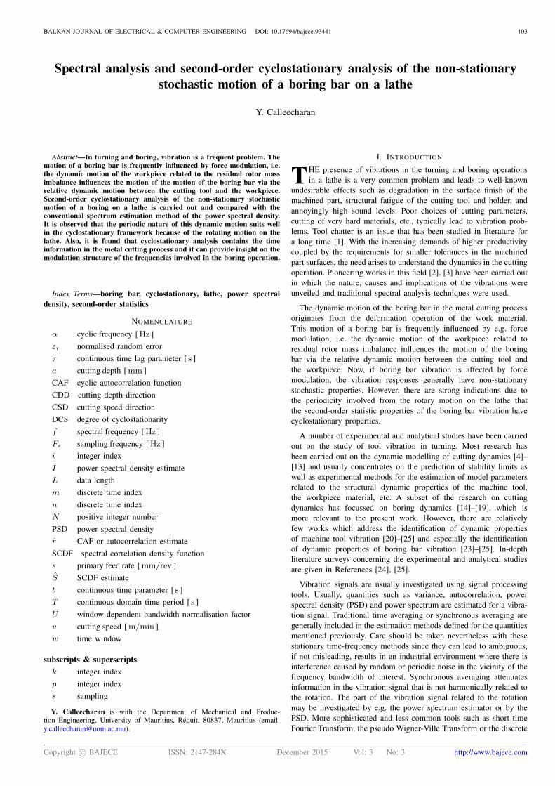
cutting operations have been carried out in a Mazak SUPER QUICK
TURN—250M CNC turning center shown in Fig. 1 with 18.5 kW
spindle power, maximal machining diameter 300 mm and 1007 mm
between the centres. In order to save material, the cutting operation
was performed as external turning operation, although a boring bar,
WIDAX S40T PDUNR15, was used.
A. Measuring equipment and setup
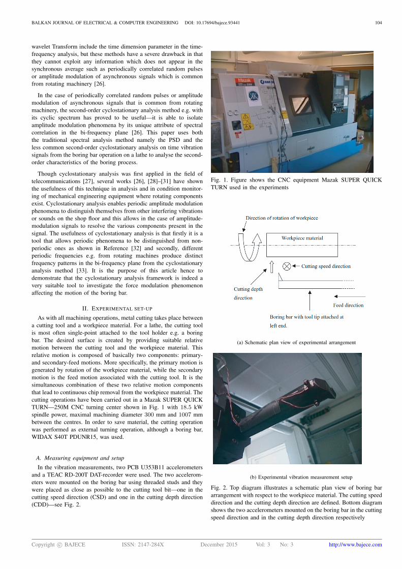
In the vibration measurements, two PCB U353B11 accelerometers
and a TEAC RD-200T DAT-recorder were used. The two accelerom-
eters were mounted on the boring bar using threaded studs and they
were placed as close as possible to the cutting tool bit—one in the
cutting speed direction (CSD) and one in the cutting depth direction
(CDD)—see Fig. 2.
Fig. 1. Figure shows the CNC equipment Mazak SUPER QUICK
TURN used in the experiments
(a) Schematic plan view of experimental arrangement
(b) Experimental vibration measurement setup
Fig. 2. Top diagram illustrates a schematic plan view of boring bar
arrangement with respect to the workpiece material. The cutting speed
direction and the cutting depth direction are defined. Bottom diagram
shows the two accelerometers mounted on the boring bar in the cutting
speed direction and in the cutting depth direction respectively
Copyright c© BAJECE ISSN: 2147-284X December 2015 Vol: 3 No: 3 http://www.bajece.com
BALKAN JOURNAL OF ELECTRICAL & COMPUTER ENGINEERING DOI: 10.17694/bajece.93441 105
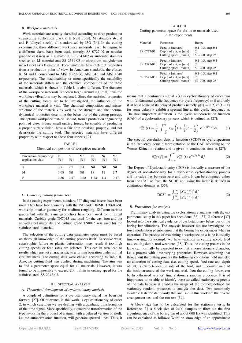
B. Workpiece materials
Work materials are usually classified according to three production
engineering application classes: K (cast irons), M (stainless steels)
and P (alloyed steels), all standardised by ISO [34]. In the cutting
experiments, three different workpiece materials, each belonging to
a different class, have been used, namely: SS 0727-02 or nodular
graphite cast iron as a K material, SS 2343-02 or austenitic stainless
steel as an M material and SS 2541-03 or chromium molybdenum
nickel steel as a P material. These materials have different properties
from a production point of view. In American standards, the classes
K, M and P correspond to AISI 80-55-06, AISI 316 and AISI 4340
respectively. The machinability or more specifically the cuttability
of the materials differs and the chemical composition of the three
materials, which is shown in Table I, is also different. The diameter
of the workpiece materials is chosen large (around 200 mm); thus the
workpiece vibrations may be neglected. Since the statistical properties
of the cutting forces are to be investigated, the influence of the
workpiece material is vital. The chemical composition and micro-
structure of the materials as well as the strength and the thermo-
dynamical properties determine the behaviour of the cutting process.
The optimal workpiece material should, from a production engineering
point of view, induce small cutting forces, be capable of producing
a proper surface finish, have a fair chip breaking property, and not
deteriorate the cutting tool. The selected materials have different
properties with respect to these four aspects [21].
TABLE I
Chemical composition of workpiece materials
Production engineering C Si Mn Cr Ni Moapplication class [%] [%] [%] [%] [%] [%]
K 3.7 2.2 0.4 Nil Nil Nil
M 0.05 Nil Nil 18 12 2.7
P 0.36 0.27 0.62 1.53 1.41 0.17
C. Choice of cutting parameters
In the cutting experiments, standard 55◦ diagonal inserts have been
used. They have tool geometry with the ISO code DNMG 150608-SL
with chip breaker geometry for medium roughing. Different carbide
grades but with the same geometries have been used for different
materials. Carbide grade TN7015 was used for the cast iron and the
alloyed steel materials, and carbide grade TN8025 was used for the
stainless steel material.
The selection of the cutting data parameter space must be based
on thorough knowledge of the cutting process itself. Excessive wear,
catastrophic failure or plastic deformation may result if too high
cutting speeds or feed rates are selected. This can in turn lead to
results which are not characteristic to a turning operation under normal
circumstances. The cutting data were chosen according to Table II.
Also, no cutting fluid was applied during machining. The aim was
to find a parameter space equal for all materials. However, it was
found to be impossible to exceed 200 m/min in cutting speed for the
stainless steel SS 2343-02.
III. SPECTRAL ANALYSIS
A. Theoretical development of cyclostationary analysis
A couple of definitions for a cyclostationary signal has been put
forward [27]. Of relevance in this work is cyclostationarity of order
2, in which case then we are dealing with a quadratic transformation
of the time signal. More specifically, a quadratic transformation of the
type involving the product of a signal with a delayed version of itself,
i.e. the autocorrelation function, will generate spectral lines. Thus, it
TABLE II
Cutting parameter space for the three materials used
in the experiments
Material Parameter Range
Feed, s [mm/rev] 0.1–0.3, step 0.1SS 0727-02 Depth of cut, a [mm] 2
Cutting speed [m/min] 50–300, step 25
Feed, s [mm/rev] 0.1–0.3, step 0.1SS 2343-02 Depth of cut, a [mm] 2
Cutting speed [m/min] 50–200, step 25
Feed, s [mm/rev] 0.1–0.3, step 0.1SS 2541-03 Depth of cut, a [mm] 2
Cutting speed [m/min] 50–300, step 25
means that a continuous signal x(t) is cyclostationary of order two
with fundamental cyclic frequency (or cycle frequency) α if and only
if at least some of its delayed products namely y(t) = x(t)x∗(t− τ)for some delays τ exhibit a spectral line at this cyclic frequency α.
The next important definition is the cyclic autocorrelation function
(CAF) of a cyclostationary process which is defined as [27]:
rαkxx
(t) =1
T
∫ T2
−T2
rxx
(
t+t
2, t−
t
2
)
e−j2pαkt dt (1)
The spectral correlation density function (SCDF) or cyclic spectrum
is the frequency domain representation of the CAF according to the
Wiener-Khinchin relation and is given in continuous time as [27]:
Sαkxx
(f) =
∫
∞
−∞
rαkxx
(t) e−j2pft
df (2)
The Degree of Cyclostationarity (DCS) is basically a measure of the
degree of non-stationarity for a wide-sense cyclostationary process
and its value lies between zero and unity. It can be computed either
from the CAF or from the SCDF, and using the latter is defined in
continuous domain as [35]:
DCSα =
∫
∞
−∞|Sα
xx(f)|2 df
∫
∞
−∞|S0
xx(f)|2 df
(3)
B. Procedures for analysis
Preliminary analysis using the cyclostationary analysis with the ex-
perimental setup in this paper has been done [36], [37]. Reference [37]
looked into the statistical evidence of cyclostationary behaviour of the
boring bar vibrations. The analysis however did not investigate the
force modulation phenomenon that the boring bar experiences when in
operation. The process of machining a workpiece on a lathe is usually
time-varying; for example we have variation in cutting speed, feed
rate, cutting depth, tool wear, etc. [38]. Thus, the cutting process in the
lathe can normally be expected to exhibit a non-stationary character,
i.e. a process with time-varying properties. However, assuming that
throughout the cutting process the following conditions hold namely:
no alteration of cutting data (i.e. cutting speed, feed rate and depth
of cut), slow deterioration rate of the tool, and time-invariance of
the basic structure of the work material, then the cutting forces can
be hypothesised as short time stationary random processes. It is of
importance to be able to identify these so-called stationary segments
of the data because it enables the usage of the toolbox defined for
stationary random processes to analyse the data. Two commonly
available tests for stationarity that are used in this work are the reverse
arrangement test and the run test [39].
A block size has to be calculated for the stationary tests. In
Reference [3], a block size of 2400 samples to filter out the first
eigenfrequency of the boring bar of about 600 Hz was identified. This
can be explained as follows: With the knowledge of an approximate
Copyright c© BAJECE ISSN: 2147-284X December 2015 Vol: 3 No: 3 http://www.bajece.com
BALKAN JOURNAL OF ELECTRICAL & COMPUTER ENGINEERING DOI: 10.17694/bajece.93441 106
value of 600 Hz for the first eigenfrequency (in either CSD or CDD)
and a sampling frequency Fs of 48 kHz, it can be readily observed
that, choosing a block size of 2400 samples, the number of periods
of this 600-Hz-eigenfrequency is 30 (in this 2400 samples). This
value of 30 averages was considered sufficient to average out the
eigenfrequency effect and it is important to note that in order not
to interfere with any other phenomenon (periodic or not) present in
the data, it is essential not to use more averages than necessary. This
block size of 2400 samples corresponds to an averaging time of 0.05 s.
Amplitude-modulated vibration signals emanating from rotating ma-
chinery generally involve harmonics of the rotating component. It
is obvious that if the spindle rotation frequency is filtered out by
some averaging time, then so are its harmonics. A simple and most
straightforward method to achieve this is to increase the block size
(from the 2400 samples) until we cannot observe any fluctuating trend
in the mean square values. The optimum block size, in this respect,
to filter out the low spindle rotation frequency of around 6 Hz was
found to be 96 000 samples, implying an averaging time of 2 s.
Cyclostationarity (in the wide sense) implies periodic variation in
the second-order characteristics, hence in the mean square values also.
Now from the previous paragraph, it is clear that using a block size
of 96 000 samples filters or smoothes out any periodic fluctuations in
the mean square values. Therefore, it is obvious that any stationary
segments identified in the time data record will contain cyclostationary
components as well. It is useful to note that since the two stationarity
tests rest on the normal distribution assumption, the minimum number
of observations has been set to a value of 10. Also here, it is useful
to point out that the level of significance was set to 0.05 and this
irrespective of the number of observations. A Matlab [40] script has
been written, the purpose of which is to help identifying stationary
segments in the time data records and identifying the longest possible
stationary segment so that in the analysis, we are sure to obtain the
most reliable spectral estimates, be it with the PSD or with the cyclic
spectrum in the cyclostationary analysis.
1) Selection of vibration data for analysis
A suitable approach had to be found to identify data that will most
probably be of interest in the cyclostationary analysis. The essential
steps in this selection procedure for each of the boring bar vibration
data were to:
1) Identify the longest stationary segment in the data using the
reverse arrangement test and the run test.
2) Compute the PSD in a frequency region around the first eigen-
frequency of the boring bar (which is around 600 Hz in either
CDD or CSD) over this longest stationary segment.
3) In the event that the PSD from Step 2 displays sufficient
amplitude-modulation phenomenon (in the form of sidebands
in the frequency region around the eigenfrequency), then the
boring bar vibration data is considered as a potential candidate
for cyclostationary analysis.
Having identified potential candidates for analysis, the next step
was to compute the DCS function. The DCS function is expected to
exhibit sufficient energy at α other than zero at twice the low spindle
rotation frequency and also at high frequencies around twice the first
eigenfrequency (assuming that these two frequency components are
mainly responsible for the vibration of the boring bar). If the DCS
does not show these features, the vibration data is discarded. It was
not timely possible to investigate each of the boring bar vibration data,
but it has been found in general that data with the highest primary feed
rate of s = 0.3 mm/rev had the desired features. In this respect, data
pertaining to this high feed-rate was investigated for various cutting
speeds and for the three different workpiece materials mentioned in
Table II, and the normalised random error was computed according
to Reference [27].
2) Estimation of PSD
The Welch method [41] has been used for the computation of the
PSD. The pth periodogram of length N1 with the use of windows is
given by
Ipxx
(fk) =Ts
N1 U
∣
∣
∣
∣
∣
N1−1∑
i=0
xp(i)w(i)e−j
2 p k nN1
∣
∣
∣
∣
∣
2
, 0 ≤ p ≤ N2 − 1
(4)
where fk is given by fk = kN1 Ts
and
U =1
N1
N1−1∑
n=0
(
w(n))2
(5)
is the window-dependent resolution bandwidth normalisation fac-
tor [42] for PSD estimation. Finally, the Welch estimate, Ixx, is the
average of all the periodograms over all segments N2 as follows:
Ixx (fk) =1
N2
N2−1∑
p=0
I(p)xx
(fk) (6)
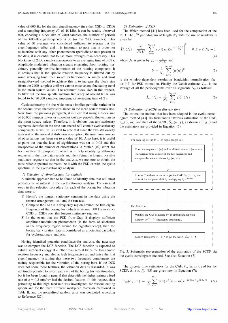
3) Estimation of SCDF in discrete time
The estimation method that has been adopted is the cyclic correl-
ogram method [43]. Its formulation involves estimation of the CAF,
rxx (α, m), and then of the SCDF, Sxx (α, f), as shown in Fig. 3 and
the estimators are provided in Equation (7).
For each lag m (up to L ≪ signal length N )
Form the sequence x(n) and its shifted version x(n − m).
Rectangular time-windowed the two sequences and
compute the autocorrelation rxx (n, m).
Fourier Transform n → α to get the CAF rxx (α, m) and
correct for the phase shift by multiplying by ejpαm.
For desired α
Window the CAF sequence by an appropriate tapering
window w(2L−1) (frequency smoothing).
Fourier Transform m → f to get the SCDF Sxx (α, f).
Fig. 3. Schematic representation of the estimation of the SCDF via
the cyclic correlogram method. See also Equation (7)
The discrete time estimators for the CAF, rxx (α, m), and for the
SCDF, Sxx (α, f), [43] are given next in Equation (7):
rxx (αk, m) =1
N
N−1∑
n=0
x(n)x∗(n − m) e−j2pαkn e
jpakm (7a)
Copyright c© BAJECE ISSN: 2147-284X December 2015 Vol: 3 No: 3 http://www.bajece.com
BALKAN JOURNAL OF ELECTRICAL & COMPUTER ENGINEERING DOI: 10.17694/bajece.93441 107
Sxx (αk, fk) =1
N
L∑
m=−L
w(2L−1)(m)
[
x(n)x∗(n−m) e−j2pαkn e
jpαkm]
e−j2pkm2L+1 (7b)
with the cyclic frequency αk = k 1Ts
, k = 0,±1,±2, . . . and 1Ts
is
the fundamental frequency. It is readily apparent that when αk = 0,
Equation (7a) reduces to the conventional autocorrelation function.
Also, then a generally non-stationary process is said to exhibit
cyclostationarity in the wide sense only if there exists correlation
between some frequency-shifted versions of the process as opposed
to a stationary process which exhibits no correlation between any
frequency-shifted versions of the process.
In the computation of the CAF, a rectangular window was applied
to the time shifted sequences. Similarly, in the computation of the
SCDF (see Equation (7b)), a suitable window needs to be applied
prior taking the Fourier Transform with respect to m. A symmetric
window with tapering ends and having unity magnitude at m = 0has the advantage of de-emphasising the unreliable parts of the CAF,
thus reducing the variance in the computation of the SCDF. Thus in
Equation (7b), the window w, with support [−L, L] and of length
2L − 1, is applied to the CAF sequence which has been calculated
using Equation (7a) for both positive and negative lags k. The negative
CAF values are obtained from the positive counterparts by exploiting
the symmetry property of the CAF.
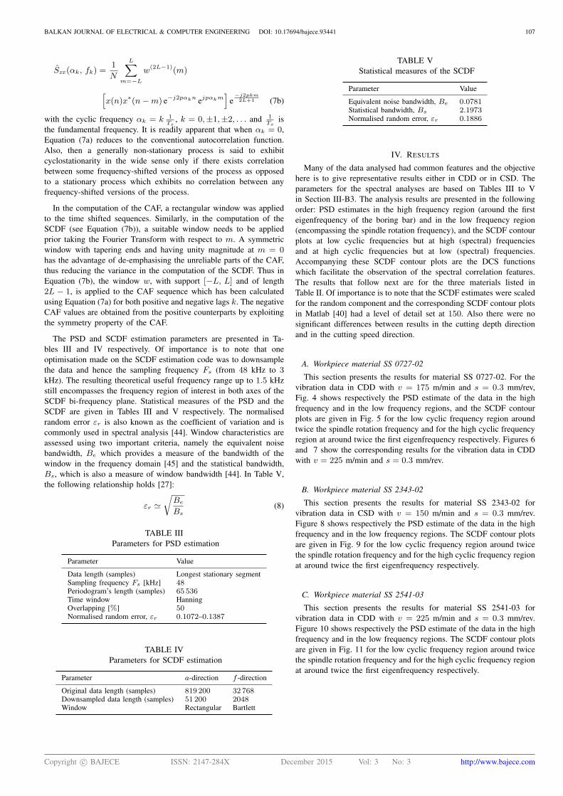
The PSD and SCDF estimation parameters are presented in Ta-
bles III and IV respectively. Of importance is to note that one
optimisation made on the SCDF estimation code was to downsample
the data and hence the sampling frequency Fs (from 48 kHz to 3kHz). The resulting theoretical useful frequency range up to 1.5 kHz
still encompasses the frequency region of interest in both axes of the
SCDF bi-frequency plane. Statistical measures of the PSD and the
SCDF are given in Tables III and V respectively. The normalised
random error εr is also known as the coefficient of variation and is
commonly used in spectral analysis [44]. Window characteristics are
assessed using two important criteria, namely the equivalent noise
bandwidth, Be which provides a measure of the bandwidth of the
window in the frequency domain [45] and the statistical bandwidth,
Bs, which is also a measure of window bandwidth [44]. In Table V,
the following relationship holds [27]:
εr ≃
√
Be
Bs
(8)
TABLE III
Parameters for PSD estimation
Parameter Value
Data length (samples) Longest stationary segmentSampling frequency Fs [kHz] 48
Periodogram’s length (samples) 65 536
Time window HanningOverlapping [%] 50
Normalised random error, εr 0.1072–0.1387
TABLE IV
Parameters for SCDF estimation
Parameter a-direction f -direction
Original data length (samples) 819 200 32 768
Downsampled data length (samples) 51 200 2048
Window Rectangular Bartlett
TABLE V
Statistical measures of the SCDF
Parameter Value
Equivalent noise bandwidth, Be 0.0781Statistical bandwidth, Bs 2.1973Normalised random error, εr 0.1886
IV. RESULTS
Many of the data analysed had common features and the objective
here is to give representative results either in CDD or in CSD. The
parameters for the spectral analyses are based on Tables III to V
in Section III-B3. The analysis results are presented in the following
order: PSD estimates in the high frequency region (around the first
eigenfrequency of the boring bar) and in the low frequency region
(encompassing the spindle rotation frequency), and the SCDF contour
plots at low cyclic frequencies but at high (spectral) frequencies
and at high cyclic frequencies but at low (spectral) frequencies.
Accompanying these SCDF contour plots are the DCS functions
which facilitate the observation of the spectral correlation features.
The results that follow next are for the three materials listed in
Table II. Of importance is to note that the SCDF estimates were scaled
for the random component and the corresponding SCDF contour plots
in Matlab [40] had a level of detail set at 150. Also there were no
significant differences between results in the cutting depth direction
and in the cutting speed direction.
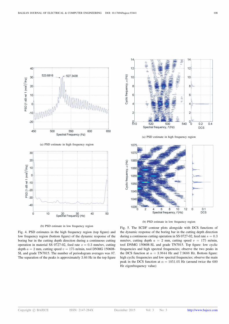
A. Workpiece material SS 0727-02
This section presents the results for material SS 0727-02. For the
vibration data in CDD with v = 175 m/min and s = 0.3 mm/rev,
Fig. 4 shows respectively the PSD estimate of the data in the high
frequency and in the low frequency regions, and the SCDF contour
plots are given in Fig. 5 for the low cyclic frequency region around
twice the spindle rotation frequency and for the high cyclic frequency
region at around twice the first eigenfrequency respectively. Figures 6
and 7 show the corresponding results for the vibration data in CDD
with v = 225 m/min and s = 0.3 mm/rev.
B. Workpiece material SS 2343-02
This section presents the results for material SS 2343-02 for
vibration data in CSD with v = 150 m/min and s = 0.3 mm/rev.
Figure 8 shows respectively the PSD estimate of the data in the high
frequency and in the low frequency regions. The SCDF contour plots
are given in Fig. 9 for the low cyclic frequency region around twice
the spindle rotation frequency and for the high cyclic frequency region
at around twice the first eigenfrequency respectively.
C. Workpiece material SS 2541-03
This section presents the results for material SS 2541-03 for
vibration data in CDD with v = 225 m/min and s = 0.3 mm/rev.
Figure 10 shows respectively the PSD estimate of the data in the high
frequency and in the low frequency regions. The SCDF contour plots
are given in Fig. 11 for the low cyclic frequency region around twice
the spindle rotation frequency and for the high cyclic frequency region
at around twice the first eigenfrequency respectively.
Copyright c© BAJECE ISSN: 2147-284X December 2015 Vol: 3 No: 3 http://www.bajece.com
BALKAN JOURNAL OF ELECTRICAL & COMPUTER ENGINEERING DOI: 10.17694/bajece.93441 108
(a) PSD estimate in high frequency region
(b) PSD estimate in low frequency region
Fig. 4. PSD estimates in the high frequency region (top figure) and
low frequency region (bottom figure) of the dynamic response of the
boring bar in the cutting depth direction during a continuous cutting
operation in material SS 0727-02, feed rate s = 0.3 mm/rev, cutting
depth a = 2 mm, cutting speed v = 175 m/min, tool DNMG 150608-
SL and grade TN7015. The number of periodogram averages was 87.
The separation of the peaks is approximately 3.66 Hz in the top figure
(a) PSD estimate in high frequency region
(b) PSD estimate in low frequency region
Fig. 5. The SCDF contour plots alongside with DCS functions of
the dynamic response of the boring bar in the cutting depth direction
during a continuous cutting operation in SS 0727-02, feed rate s = 0.3mm/rev, cutting depth a = 2 mm, cutting speed v = 175 m/min,
tool DNMG 150608-SL and grade TN7015. Top figure: low cyclic
frequencies and high spectral frequencies; observe the two peaks in
the DCS function at α = 3.9844 Hz and 7.9688 Hz. Bottom figure:
high cyclic frequencies and low spectral frequencies; observe the main
peak in the DCS function at α = 1051.05 Hz (around twice the 600Hz eigenfrequency value)
Copyright c© BAJECE ISSN: 2147-284X December 2015 Vol: 3 No: 3 http://www.bajece.com
BALKAN JOURNAL OF ELECTRICAL & COMPUTER ENGINEERING DOI: 10.17694/bajece.93441 109
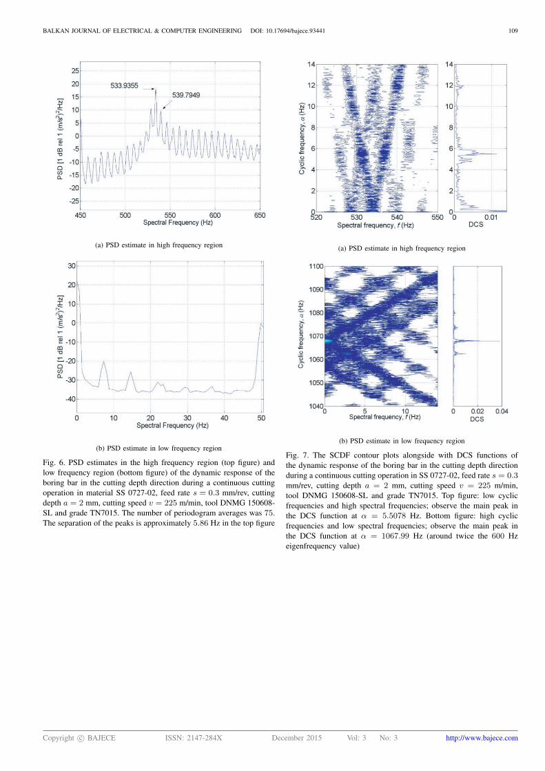
(a) PSD estimate in high frequency region
(b) PSD estimate in low frequency region
Fig. 6. PSD estimates in the high frequency region (top figure) and
low frequency region (bottom figure) of the dynamic response of the
boring bar in the cutting depth direction during a continuous cutting
operation in material SS 0727-02, feed rate s = 0.3 mm/rev, cutting
depth a = 2 mm, cutting speed v = 225 m/min, tool DNMG 150608-
SL and grade TN7015. The number of periodogram averages was 75.
The separation of the peaks is approximately 5.86 Hz in the top figure
(a) PSD estimate in high frequency region
(b) PSD estimate in low frequency region
Fig. 7. The SCDF contour plots alongside with DCS functions of
the dynamic response of the boring bar in the cutting depth direction
during a continuous cutting operation in SS 0727-02, feed rate s = 0.3mm/rev, cutting depth a = 2 mm, cutting speed v = 225 m/min,
tool DNMG 150608-SL and grade TN7015. Top figure: low cyclic
frequencies and high spectral frequencies; observe the main peak in
the DCS function at α = 5.5078 Hz. Bottom figure: high cyclic
frequencies and low spectral frequencies; observe the main peak in
the DCS function at α = 1067.99 Hz (around twice the 600 Hz
eigenfrequency value)
Copyright c© BAJECE ISSN: 2147-284X December 2015 Vol: 3 No: 3 http://www.bajece.com
BALKAN JOURNAL OF ELECTRICAL & COMPUTER ENGINEERING DOI: 10.17694/bajece.93441 110
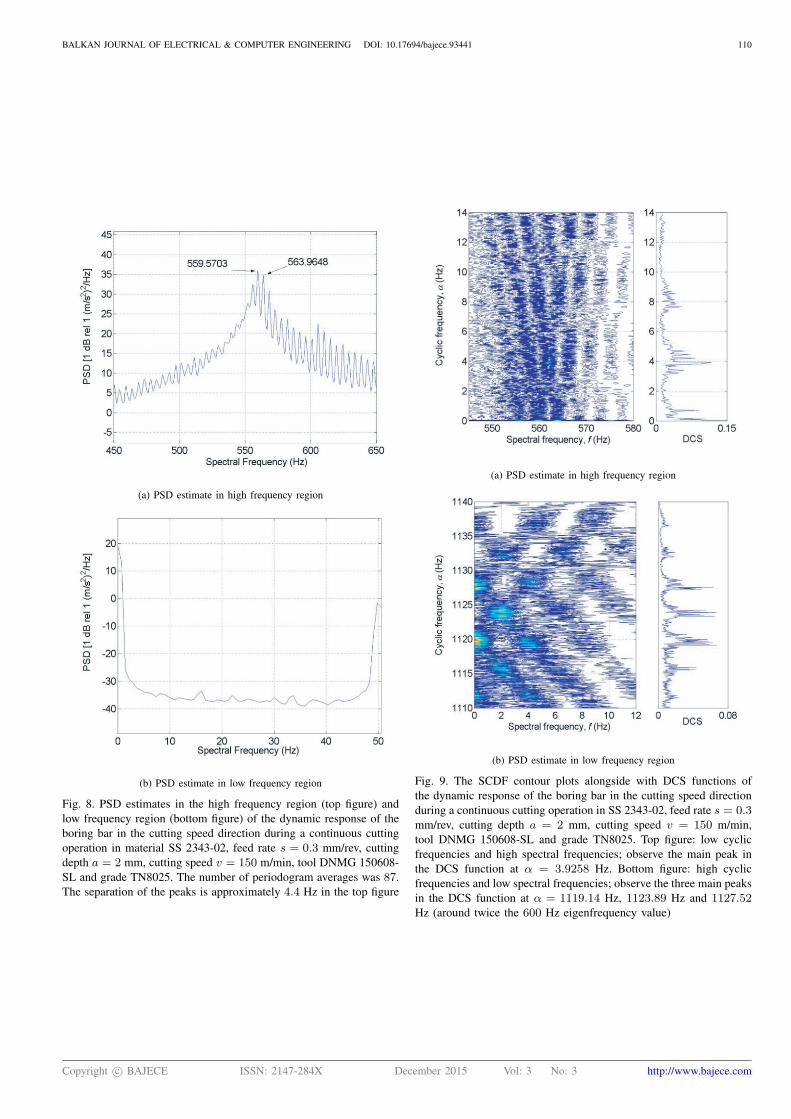
(a) PSD estimate in high frequency region
(b) PSD estimate in low frequency region
Fig. 8. PSD estimates in the high frequency region (top figure) and
low frequency region (bottom figure) of the dynamic response of the
boring bar in the cutting speed direction during a continuous cutting
operation in material SS 2343-02, feed rate s = 0.3 mm/rev, cutting
depth a = 2 mm, cutting speed v = 150 m/min, tool DNMG 150608-
SL and grade TN8025. The number of periodogram averages was 87.
The separation of the peaks is approximately 4.4 Hz in the top figure
(a) PSD estimate in high frequency region
(b) PSD estimate in low frequency region
Fig. 9. The SCDF contour plots alongside with DCS functions of
the dynamic response of the boring bar in the cutting speed direction
during a continuous cutting operation in SS 2343-02, feed rate s = 0.3mm/rev, cutting depth a = 2 mm, cutting speed v = 150 m/min,
tool DNMG 150608-SL and grade TN8025. Top figure: low cyclic
frequencies and high spectral frequencies; observe the main peak in
the DCS function at α = 3.9258 Hz. Bottom figure: high cyclic
frequencies and low spectral frequencies; observe the three main peaks
in the DCS function at α = 1119.14 Hz, 1123.89 Hz and 1127.52Hz (around twice the 600 Hz eigenfrequency value)
Copyright c© BAJECE ISSN: 2147-284X December 2015 Vol: 3 No: 3 http://www.bajece.com
BALKAN JOURNAL OF ELECTRICAL & COMPUTER ENGINEERING DOI: 10.17694/bajece.93441 111
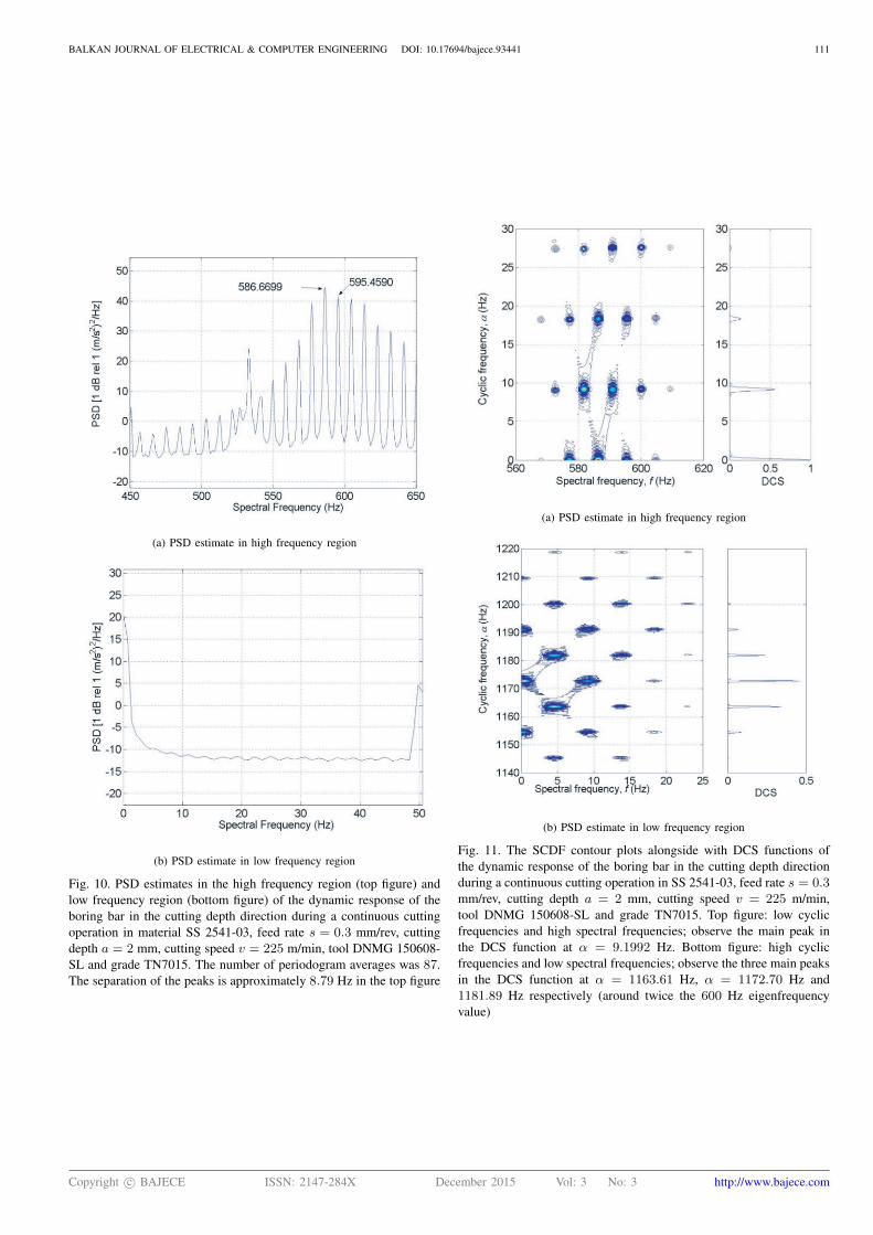
(a) PSD estimate in high frequency region
(b) PSD estimate in low frequency region
Fig. 10. PSD estimates in the high frequency region (top figure) and
low frequency region (bottom figure) of the dynamic response of the
boring bar in the cutting depth direction during a continuous cutting
operation in material SS 2541-03, feed rate s = 0.3 mm/rev, cutting
depth a = 2 mm, cutting speed v = 225 m/min, tool DNMG 150608-
SL and grade TN7015. The number of periodogram averages was 87.
The separation of the peaks is approximately 8.79 Hz in the top figure
(a) PSD estimate in high frequency region
(b) PSD estimate in low frequency region
Fig. 11. The SCDF contour plots alongside with DCS functions of
the dynamic response of the boring bar in the cutting depth direction
during a continuous cutting operation in SS 2541-03, feed rate s = 0.3mm/rev, cutting depth a = 2 mm, cutting speed v = 225 m/min,
tool DNMG 150608-SL and grade TN7015. Top figure: low cyclic
frequencies and high spectral frequencies; observe the main peak in
the DCS function at α = 9.1992 Hz. Bottom figure: high cyclic
frequencies and low spectral frequencies; observe the three main peaks
in the DCS function at α = 1163.61 Hz, α = 1172.70 Hz and
1181.89 Hz respectively (around twice the 600 Hz eigenfrequency
value)
Copyright c© BAJECE ISSN: 2147-284X December 2015 Vol: 3 No: 3 http://www.bajece.com
BALKAN JOURNAL OF ELECTRICAL & COMPUTER ENGINEERING DOI: 10.17694/bajece.93441 112
V. DISCUSSIONS AND ANALYSES
In the PSD estimates of the boring bar vibration data, there seems
to be a correlation between the adjacent sideband distance and the
workpiece rotation frequency. This might suggest that workpiece
motion at the rotation frequency amplitude modulates the response
of the boring bar at its first eigenfrequency.
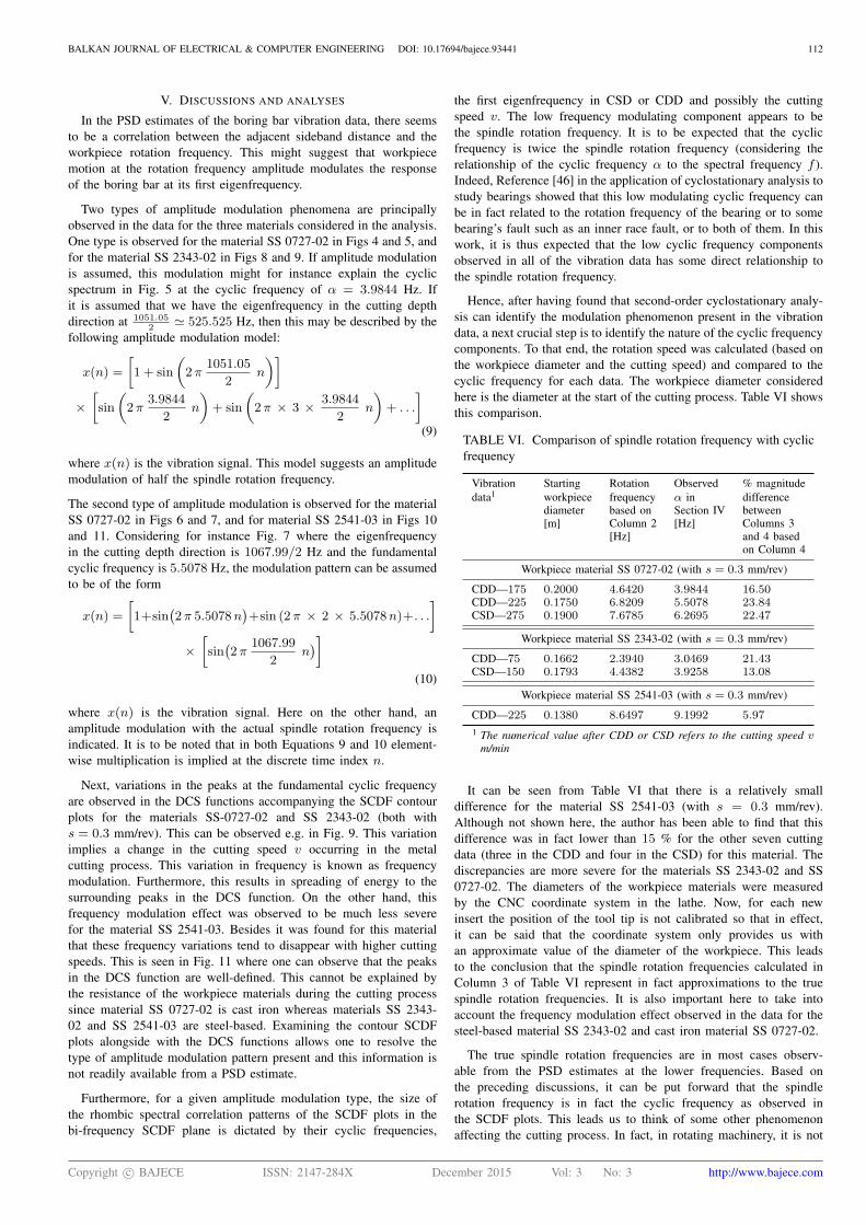
Two types of amplitude modulation phenomena are principally
observed in the data for the three materials considered in the analysis.
One type is observed for the material SS 0727-02 in Figs 4 and 5, and
for the material SS 2343-02 in Figs 8 and 9. If amplitude modulation
is assumed, this modulation might for instance explain the cyclic
spectrum in Fig. 5 at the cyclic frequency of α = 3.9844 Hz. If
it is assumed that we have the eigenfrequency in the cutting depth
direction at 1051.052
≃ 525.525 Hz, then this may be described by the
following amplitude modulation model:
x(n) =
[
1 + sin
(
2π1051.05
2n
)]
×
[
sin
(
2π3.9844
2n
)
+ sin
(
2π × 3 ×3.9844
2n
)
+ . . .
]
(9)
where x(n) is the vibration signal. This model suggests an amplitude
modulation of half the spindle rotation frequency.
The second type of amplitude modulation is observed for the material
SS 0727-02 in Figs 6 and 7, and for material SS 2541-03 in Figs 10
and 11. Considering for instance Fig. 7 where the eigenfrequency
in the cutting depth direction is 1067.99/2 Hz and the fundamental
cyclic frequency is 5.5078 Hz, the modulation pattern can be assumed
to be of the form
x(n) =
[
1+sin(
2π 5.5078n)
+sin (2π × 2 × 5.5078n)+. . .
]
×
[
sin(
2π1067.99
2n)
]
(10)
where x(n) is the vibration signal. Here on the other hand, an
amplitude modulation with the actual spindle rotation frequency is
indicated. It is to be noted that in both Equations 9 and 10 element-
wise multiplication is implied at the discrete time index n.
Next, variations in the peaks at the fundamental cyclic frequency
are observed in the DCS functions accompanying the SCDF contour
plots for the materials SS-0727-02 and SS 2343-02 (both with
s = 0.3 mm/rev). This can be observed e.g. in Fig. 9. This variation
implies a change in the cutting speed v occurring in the metal
cutting process. This variation in frequency is known as frequency
modulation. Furthermore, this results in spreading of energy to the
surrounding peaks in the DCS function. On the other hand, this
frequency modulation effect was observed to be much less severe
for the material SS 2541-03. Besides it was found for this material
that these frequency variations tend to disappear with higher cutting
speeds. This is seen in Fig. 11 where one can observe that the peaks
in the DCS function are well-defined. This cannot be explained by
the resistance of the workpiece materials during the cutting process
since material SS 0727-02 is cast iron whereas materials SS 2343-
02 and SS 2541-03 are steel-based. Examining the contour SCDF
plots alongside with the DCS functions allows one to resolve the
type of amplitude modulation pattern present and this information is
not readily available from a PSD estimate.
Furthermore, for a given amplitude modulation type, the size of
the rhombic spectral correlation patterns of the SCDF plots in the
bi-frequency SCDF plane is dictated by their cyclic frequencies,
the first eigenfrequency in CSD or CDD and possibly the cutting
speed v. The low frequency modulating component appears to be
the spindle rotation frequency. It is to be expected that the cyclic
frequency is twice the spindle rotation frequency (considering the
relationship of the cyclic frequency α to the spectral frequency f ).
Indeed, Reference [46] in the application of cyclostationary analysis to
study bearings showed that this low modulating cyclic frequency can
be in fact related to the rotation frequency of the bearing or to some
bearing’s fault such as an inner race fault, or to both of them. In this
work, it is thus expected that the low cyclic frequency components
observed in all of the vibration data has some direct relationship to
the spindle rotation frequency.
Hence, after having found that second-order cyclostationary analy-
sis can identify the modulation phenomenon present in the vibration
data, a next crucial step is to identify the nature of the cyclic frequency
components. To that end, the rotation speed was calculated (based on
the workpiece diameter and the cutting speed) and compared to the
cyclic frequency for each data. The workpiece diameter considered
here is the diameter at the start of the cutting process. Table VI shows
this comparison.
TABLE VI. Comparison of spindle rotation frequency with cyclic
frequency
Vibration Starting Rotation Observed % magnitude
data1 workpiece frequency α in differencediameter based on Section IV between[m] Column 2 [Hz] Columns 3
[Hz] and 4 basedon Column 4
Workpiece material SS 0727-02 (with s = 0.3 mm/rev)
CDD—175 0.2000 4.6420 3.9844 16.50CDD—225 0.1750 6.8209 5.5078 23.84CSD—275 0.1900 7.6785 6.2695 22.47
Workpiece material SS 2343-02 (with s = 0.3 mm/rev)
CDD—75 0.1662 2.3940 3.0469 21.43CSD—150 0.1793 4.4382 3.9258 13.08
Workpiece material SS 2541-03 (with s = 0.3 mm/rev)
CDD—225 0.1380 8.6497 9.1992 5.97
1 The numerical value after CDD or CSD refers to the cutting speed vm/min
It can be seen from Table VI that there is a relatively small
difference for the material SS 2541-03 (with s = 0.3 mm/rev).
Although not shown here, the author has been able to find that this
difference was in fact lower than 15 % for the other seven cutting
data (three in the CDD and four in the CSD) for this material. The
discrepancies are more severe for the materials SS 2343-02 and SS
0727-02. The diameters of the workpiece materials were measured
by the CNC coordinate system in the lathe. Now, for each new
insert the position of the tool tip is not calibrated so that in effect,
it can be said that the coordinate system only provides us with
an approximate value of the diameter of the workpiece. This leads
to the conclusion that the spindle rotation frequencies calculated in
Column 3 of Table VI represent in fact approximations to the true
spindle rotation frequencies. It is also important here to take into
account the frequency modulation effect observed in the data for the
steel-based material SS 2343-02 and cast iron material SS 0727-02.
The true spindle rotation frequencies are in most cases observ-
able from the PSD estimates at the lower frequencies. Based on
the preceding discussions, it can be put forward that the spindle
rotation frequency is in fact the cyclic frequency as observed in
the SCDF plots. This leads us to think of some other phenomenon
affecting the cutting process. In fact, in rotating machinery, it is not
Copyright c© BAJECE ISSN: 2147-284X December 2015 Vol: 3 No: 3 http://www.bajece.com
BALKAN JOURNAL OF ELECTRICAL & COMPUTER ENGINEERING DOI: 10.17694/bajece.93441 113
uncommon to observe that looseness in some fixtures manifests itself
by a sideband at half the rotation frequency of the main rotating
component [47]. The fact that the cutting speed varies during cutting
and that the SCDF plots suggest either an amplitude modulation of
the eigenfrequency with half the workpiece rotation frequency or with
the actual workpiece rotation frequency leads to the conclusion that
the structure of the boring bar vibration is more complex than the
hypothesised simple amplitude modulation structure.
VI. CONCLUSIONS
The objective of this work is to investigate the force modulation
phenomenon associated with the dynamic motion of the boring bar
in the metal cutting process on a lathe. In Reference [3] it has been
shown that the effect of the material deformation process is to induce
vibration in the boring bar at the first eigenfrequency in either CDD or
CSD. Unbalance in the workpiece rotation was also known to affect
the vibrations of the boring bar. The stochastic nature of the cutting
process is exposed by the PSD analysis, but the latter is limited in
analysis by its time-invariance property.
As seen in Sections IV and V, the PSD analysis has proved
to be not quite effective in revealing whether there is modulation
phenomenon occurring in the vibration data nor the exact form in
case of occurrence of amplitude modulation. In the second-order
cyclostationary analysis, the DCS function serves as preliminary tool
to unveil the presence of modulation in the vibration data. Also, in-
depth analysis with the SCDF bi-frequency contour plots could, in
every case considered, provide concise and unambiguous information
regarding the amplitude modulation phenomenon occurring. The DCS
function could be computed separately before computing the SCDF
which is more computationally expensive.
The results obtained in Section IV indicate that the cyclic spectrum
(or SCDF plot) is likely to provide information concerning the
frequency of the actual boring bar eigenfrequency from the force-
modulated boring bar vibration data. Moreover, the cyclostationary
analysis unwrapped new information from the cutting process. Firstly,
the cycle frequencies obtained from the analysis may indicate the
presence of looseness in the fixture of the boring bar. Secondly,
frequency variations in the peaks of the DCS functions were observed
for the materials SS 2343-02 (steel-based) and SS 0727-02 (cast iron).
This variation in the DCS peaks leads to the phenomenon of frequency
modulation, which has not been investigated further in this work. It is
known that the cutting speed varies during cutting and this coupled to
the fact that the cyclostationary analysis suggests either an amplitude
modulation of the eigenfrequency with half the workpiece rotation
frequency or with the actual workpiece rotation frequency, shows that
the amplitude modulation models put forward in Section V may not
be complete.
The manufacturing industry is always putting much effort to reduce
the vibration emanating from the metal cutting process on a lathe.
Thus, understanding the causes and sources of the vibration causing
effect is fundamental. In this work, second-order cyclostationary
analysis has revealed some looseness in the boring bar fixture; such
information is vital to the vibration control engineers. In essence,
cyclostationary analysis at the second order has demonstrated its
ability to handle the non-stationary stochastic nature of the metal
cutting process on a lathe.
ACKNOWLEDGMENTS
The author wishes to express his sincere thanks to Prof. Lars
Håkansson of the Department of Applied Signal Processing, Blekinge
Tekniska Högskola (Blekinge Institute of Technology), Sweden, for
his assistance.
REFERENCES
[1] Y. Altintas. Manufacturing Automation, Metal Cuting Mechanics, Ma-
chine Tool Vibrations, and CNC design. Cambridge University Press,2000.
[2] L. Håkansson. Adaptive Active Control of Machine-Tool Vibration in a
Lathe—Analysis and Experiments. PhD thesis, Department of Productionand Materials Engineering, Lund University, Sweden, 1999.
[3] L. Pettersson. Vibrations in metal cutting: measurement, analysis and
reduction. Licentiate thesis, Department of Telecmmunications andSignal Processing, Blekinge Institute of Technology, Sweden, 2002.
[4] J. Tlusty. Analysis of the state of research in cutting dynamics. In Annals
of the CIRP, volume 27/2, pages 583–589. CIRP, 1978.[5] D.W. Wu and C.R. Liu. An analytical model of cutting dynamics—Part
1: Model building. Journal of Engineering for Industry, Transactions of
the ASME, 107(2):107–111, May 1985.[6] D.W. Wu and C.R. Liu. An analytical model of cutting dynamics—Part
2: Verification. Journal of Engineering for Industry, Transactions of the
ASME, 107(2):112–118, May 1985.[7] I.E. Minis, E.B. Magrab, and I.O. Pandelidis. Improved methods for
the prediction of chatter in turning—Part 1: Determination of structuralresponse parameters. Journal of Engineering for Industry, Transactions
of the ASME, 112:12–20, February 1990.[8] I.E. Minis, E.B. Magrab, and I.O. Pandelidis. Improved methods for
the prediction of chatter in turning—Part 2: Determination of cuttingprocess parameters. Journal of Engineering for Industry, Transactions of
the ASME, 112:21–27, February 1990.[9] I.E. Minis, E.B. Magrab, and I.O. Pandelidis. Improved methods for
the prediction of chatter in turning—Part 3: A generalized linear theory.Journal of Engineering for Industry, Transactions of the ASME, 112:28–35, February 1990.
[10] S.M. Pandit, T.L. Subramanian, and S.M. Wu. Modeling machine toolchatter by time series. Journal of Engineering for Industry, Transactions
of the ASME, 97:211–215, February 1975.[11] S.M. Pandit, T.L. Subramanian, and S.M. Wu. Stability of random
vibrations with special reference to machine tool chatter. Journal
of Engineering for Industry, Transactions of the ASME, 97:216–219,February 1975.
[12] T. Kalmár-Nagy, G. Stépán, and F.C. Moon. Subcritical Hopf bifurcationin the delay equation model for machine tool vibrations. Journal of
Nonlinear Dynamics, 26:121–142, 2001.[13] J. Gradisek, E. Govekar, and I. Grabec. Chatter onset in non-regenerative
cutting: A numerical study. Journal of Sound and Vibration, 242(5):829–838, 2001.
[14] E.W. Parker. Dynamic stability of a cantilever boring bar with machinedflats under regenerative cutting conditions. Journal of Mechanical
Engineering Sience, 12(2):104–115, February 1970.[15] G.M. Zhang and S.G. Kapoor. Dynamic modeling and analysis of
the boring machining system. Journal of Engineering for Industry,
Transactions of the ASME, 109(3):219–226, August 1987.[16] P.N. Rao, U.R.K. Rao, and J.S. Rao. Towards improwed design of boring
bars—Part 1: Dynamic cutting force model with continuous systemanalysis for the boring bar. International Journal of Machine Tools and
Manufacture, 28(1):33–44, 1988.[17] F. Kuster and P.E. Gygax. Cutting dynamics and stability of boring bars.
CIRP Annals—Manufacturing Technology, 39(1):361–366, 1990.[18] S. Jayaram and M. Iyer. An analytical model for prediction of chatter
stability in boring. SME technical paper, (MR00-202), Society of
Manufacturing Engineers, 28:203–208, 2000.[19] I. Lazoglu, F. Atabey, and Y. Altintas. Dynamics of boring processes—
Part III: Time domain modeling. International Journal of Machine Tools
& Manufacture, 42:1567–1576, 2002.[20] M.K. Khraisheh, C. Pezeshki, and A.E. Bayoumi. Time series based
analysis for primary chatter in metal cutting. Journal of Sound and
Vibration, 180(1):67–87, 1995.[21] P-O. H. Sturesson, L. Håkansson, and I. Claesson. Identification of the
statistical properties of the cutting tool vibration in a continuous turningoperation—Correlation to structural properties. Mechanical Systems and
Signal Processing, 11(3):459–489, 1997.[22] J. Gradisek, I. Grabec, S. Siegert, and R. Friedrich. Stochastic dynamics
of metal cutting: Bifurcation phenomena in turning. Mechanical Systems
and Signal Processing, 16(5):831–840, 2002.[23] E. Marui, S. Ema, and S. Kato. Chatter vibration of lathe tools—Part 1:
General characteristics of chatter vibration. Journal of Engineering for
Industry, Transactions of the ASME, 105(2):100–106, May 1983.[24] L. Andrén, L. Håkansson, A. Brandt, and I. Claesson. Identification
of dynamic properties of boring bar vibrations in a continuous boringoperation. Mechanical Systems & Signal Processing, 18(4):869–901,2004.
Copyright c© BAJECE ISSN: 2147-284X December 2015 Vol: 3 No: 3 http://www.bajece.com
BALKAN JOURNAL OF ELECTRICAL & COMPUTER ENGINEERING DOI: 10.17694/bajece.93441 114
[25] L. Andrén, L. Håkansson, A. Brandt, and I. Claesson. Identificationof motion of cutting tool vibration in a continuous boring operation—Correlation to structural properties. Mechanical Systems & Signal
Processing, 18(4):903–927, 2004.[26] A. McCormick and A.K. Nandi. Cyclostationarity in rotating machine
vibrations. Mechanical Systems and Signal Processing, 12(2):225–242,1998.
[27] W.A. Gardner. Statistical Spectral Analysis: A Non-Probabilistic Theory.Prentice Hall, Englewood Cliffs, New York, 1987.
[28] C. Capdessus, Sidahmed. M., and J.L. Lacoume. Cyclostationary pro-cesses: Application in gear faults early diagnosis. Mechanical Systems
and Signal Processing, 14(3):371–385, 2000.[29] L. Bouillaut and M. Sidahmed. Cyclostationary approach and bilinear
approach: comparison, applications to early diagnosis for helicoptergearbox and classification method based on HOCS. Mechanical Systems
and Signal Processing, 15(5):923–943, 2001.[30] R.B. Randall, J. Antoni, and S. Chobsaard. The relationship between
spectral correlation and envelope analysis for cyclostationary machinesignals, application to ball bearing diagnostics. Mechanical Systems and
System Processing, 15(5):945–962, 2001.[31] J. Antoni, J. Danière, and F. Guillet. Effective vibration analysis of
IC engines using cyclostationarity—Part I: A methodology for conditionmonitoring. Journal of Sound and Vibration, 257(5):815–837, 2002.
[32] M. knaak and D. Filbert. Acoustical semi-blind source separation formachine monitoring. In Proc. conference Indep. Compon. Anal. Signal,pages 361–366, 2001.
[33] J. Goerlich, D. Bruckner, A. Richter, O. Strama, R.S. Thomä, andU. Trautwein. Signal analysis using spectral correlation measurement.In IEEE Instrumentation and Measurement Technology Conference, St.
Paul, U.S.A, volume 2, pages 1313–1318, May 18–21 1998.[34] Sandvik. General turning. Sandvik AB Coromant, [On-
line]. http://www2.coromant.sandvik.com/coromant/pdf/Metalworking_Products_061/tech_a_8.pdf.
[35] W.A. Gardner and G.D. Zivanovic. Degrees of cyclostationarity andtheir application to signal detection and estimation. Signal Processing,22(3):287–297, 1991.
[36] Y. Calleecharan. Cyclostationary analysis of boring bar vibration.Master’s thesis, Blekinge Institute of Technology, Sweden, ISRN: BTH-IMA-EX–2003/D-01–SE, January 2003.
[37] A.H. Brandt, L. Håkansson, and I. Claesson. Cyclostationary analysisof boring bar vibrations. In IMAC-XXII: Conference & Exposition on
Structural Dynamics. Society of Experimental Mechanics, 2004.[38] Sandvik. Modern Metal Cuting: A Practical Handbook. AB Sandvik
Coromant, 1994.[39] J.S. Bendat and A.G. Piersol. Random data: Analysis and Measurement
Procedures. John Wiley & Sons, second edition, 1986.[40] Matlab computing software, The MathWorks 2002. Version 6.5 (R13).[41] P.D. Welch. The use of Fast Fourier Transform for the estimation of
power spectra: A method based on time averaging over short, modifiedperiodograms. IEEE Transactions on Audio and Electroacoustics, Au-15(2):70–73, June 1967.
[42] F. Harris. On the use of windows for harmonic analysis with the discreteFourier Transform. In Proc. of the IEEE, volume 66, pages 51–83, 1978.
[43] W.A. Gardner. Cyclostationarity in Communications and Signal Process-
ing. IEEE Press, New Jersey, 1994.[44] J.S. Bendat and A.G. Piersol. Random Data: Analysis and Measurement
Procedures. John Wiley & Sons, third edition, 2000.[45] H. Jokinen, J. Ollila, and O. Aumala. On windowing effects in estimating
averaged periodograms of noisy signals. Measurement, 28:197–207,2000.
[46] I. Antoniadis and G. Glossiotis. Cyclostationary analysis of rolling-element bearing vibration signals. Journal of Sound and Vibration,190(3):419–447, 1996.
[47] V. Wowk. Machinery Vibration: Measurement and Analysis. McGraw-Hill, 1991.
BIOGRAPHY
Yogeshwarsing Calleecharan received the B.Eng.(Hons) degree in Mechanical Engineering fromthe University of Mauritius, Mauritius, in 2000,the M.Sc. degree in Mechanical Engineering fromBlekinge Tekniska Högskola, Sweden, in 2003, andthe Ph.D. degree in Solid Mechanics from LuleåTekniska Universitet, Sweden, in 2013. Since 2014he is a lecturer with the Mechanical and ProductionEngineering Department, University of Mauritius,Mauritius. His research interests include solid me-chanics, vibration and signal analysis, rotordynamics,
signal processing, electromechanics and software development with the Adaprogramming language.
Copyright c© BAJECE ISSN: 2147-284X December 2015 Vol: 3 No: 3 http://www.bajece.com