Embed Size (px)
Citation preview

Spectral Analysis
Spectral analysis is a means of investigating signal’s spectral content.
It is used in: optics, speech, sonar, radar, medicine, seizmology, chemistry,radioastronomy, etc.
There are
• nonparametric (classic) and
• parametric (modern)
methods.
EE 524, # 8 1

Spectral Analysis (cont.)
EE 524, # 8 2

Power Spectral Density (PSD) of Random SignalsLet {x(n)} be a wide-sense stationary random signal:
E {x(n)} = 0, r(k) = E {x(n)x∗(n− k)}.
First definition of PSD:
P (ejω) =∞∑
k=−∞
r(k)e−jωk,
r(k) =12π
∫ π
−π
P (ejω)ejωkdω.
Second definition of PSD:
P (ejω) = limN→∞
E
{1N
∣∣∣∣∣N−1∑n=0
x(n)e−jωn
∣∣∣∣∣2}
.
EE 524, # 8 3

Power averaged over frequency:
r(0) =12π
∫ π
−π
P (ejω)dω.
Remark: Since r(k) is discrete, P (ejω) is periodic, with period 2π (ω) or1 (f).
EE 524, # 8 4

Power Spectral Density of Random Signals (cont.)
Result (without proof): First and second definitions of PSD are equivalentif
limN→∞
1N
N−1∑k=−N+1
|k||r(k)| = 0
and also if ∞∑k=−∞
|r(k)| < ∞.
That is, r(k) must decay sufficiently fast!
EE 524, # 8 5

Nonparametric Methods: Periodogram and CorrelogramPeriodogram (from the second definition of PSD):
P̂P (ejω) =1N
∣∣∣∣∣N−1∑n=0
x(n)e−jωn
∣∣∣∣∣2
.
Correlogram (from the first definition of PSD):
P̂C(ejω) =N−1∑
k=−N+1
r̂(k)e−jωk
where we can use either unbiased or biased estimates of r(k):Unbiased estimate:
r̂(k) ={
1N−k
∑N−1i=k x(i)x∗(i− k), k ≥ 0,
r̂∗(−k), k < 0.
EE 524, # 8 6

Biased estimate:
r̂(k) ={
1N
∑N−1i=k x(i)x∗(i− k), k ≥ 0,
r̂∗(−k), k < 0.
The biased estimate is more reliable than the unbiased one, because itassigns lower weights to the poorer estimates of long correlation lags.
EE 524, # 8 7

Correlogram
The biased estimate is asymptotically unbiased:
limN→∞
E {r̂(k)} = limN→∞
1N
N−1∑i=k
E {x(i)x∗(i− k)}
= limN→∞
1N
N−1∑i=k
r(k)
= limN→∞
N − k
Nr(k) = r(k).
Proposition. Correlogram computed through the biased estimate of r(k)coincides with periodogram.
EE 524, # 8 8

Proof. Consider the auxiliary signal
y(m) =1√N
N−1∑k=0
x(k)ε(m− k),
where {x(k)} are considered to be fixed constants and {ε(k)} is a unit-variance white noise:
rε(m− l) = E {ε(m)ε∗(l)} = δ(m− l).
y(m) can be viewed as the output of the filter with transfer function
X(ejω) =1√N
N−1∑k=0
x(k)e−jωk.
EE 524, # 8 9

Relationship between filter input and output PSD’s:
Py(ejω) = |X(ejω)|2Pε(ejω) = |X(ejω)|2∞∑
k=−∞
rε(k)e−jωk
= |X(ejω)|2∞∑
k=−∞
δ(k)e−jωk = |X(ejω)|2
=1N
∣∣∣∣∣N−1∑n=0
x(n)e−jωn
∣∣∣∣∣2
= P̂P (ejω).
Now, we need to prove that Py(ejω) = P̂C(ejω).
EE 524, # 8 10

Observe that
ry(k) = E {y(m)y∗(m− k)}
=1N
E
{[N−1∑p=0
x(p)ε(m− p)
][N−1∑s=0
x∗(s)ε∗(m− k − s)
]}
=1N
N−1∑p=0
N−1∑s=0
x(p)x∗(s)E {ε(m− p)ε∗(m− k − s)}
=1N
N−1∑p=0
N−1∑s=0
x(p)x∗(s)δ(p− k − s)
=1N
N−1∑p=k
x(p)x∗(p− k) ={
r̂x(k), 0 ≤ k ≤ N − 1,0, k ≥ N.
biased
EE 524, # 8 11

Inserting the last result in the first definition of PSD, we obtain
Py(ejω) =∞∑
k=−∞
ry(k)e−jωk
=N−1∑
k=−N+1
r̂x(k)e−jωk = P̂C(ejω).
2
EE 524, # 8 12

Matlab Example
x(n) = A exp(j2πfsn + φ) + ε(n)
where
• fs = 0.3 - discrete-time signal frequency
• ε - zero-mean unit-variance complex Gaussian noise
• φ - random phase uniformly distributed in [0, 2π].
EE 524, # 8 13

Periodogram: A = 1, N = 100
EE 524, # 8 14

Periodogram: A = 1, N = 1000
EE 524, # 8 15

Periodogram: A = 1, N = 10000
EE 524, # 8 16

Periodogram: A = 0.1, N = 100
EE 524, # 8 17

Periodogram: A = 0.1, N = 1000
EE 524, # 8 18

Periodogram: A = 0.1, N = 10000
EE 524, # 8 19
Statistical Analysis of Periodogram
First, consider periodogram’s bias:
E {P̂P (ejω)} = E {P̂C(ejω)} =N−1∑
k=−N+1
E {r̂(k)}e−jωk.
For the biased r̂(k), we obtain
E {r̂(k)} =(
1− k
N
)r(k), k ≥ 0
and
E {r̂(k)} = E {r̂∗(−k)} =(
1 +k
N
)r(k), k < 0.
EE 524, # 8 20

Hence
E {P̂P (ejω)} =N−1∑
k=−N+1
E {r̂(k)}e−jωk
=N−1∑
k=−N+1
(1− |k|
N
)r(k)e−jωk
=∞∑
k=−∞
wB(k)r(k)e−jωk.
where wB(k) is a Bartlett (triangular) window:
wB(k) ={
1− |k|N , −N + 1 ≤ k ≤ N − 1,
0, otherwise.
EE 524, # 8 21

Statistical Analysis of Periodogram (cont.)The last equations mean
limN→∞
E {P̂P (ejω)} = limN→∞
N−1∑k=−N+1
E {r̂(k)}e−jωk
=∞∑
k=−∞
r(k)e−jωk = P (ejω) =⇒
periodogram is asymptotically unbiased estimator of PSD. For finite N ,notice that
E {P̂P (ejω)} = DTFT{wB(k)r(k)} =⇒and, hence
E {P̂P (ejω)} =12π
∫ ∞
−∞P (ejν)WB(ejω−ν)dν,
EE 524, # 8 22

P (ejω) = DTFT{r(k)}, WB(ejω) = DTFT{wB(k)}.
WB(ejω) =1N
[sin(ωN/2)sin(ω/2)
]2
.
EE 524, # 8 23
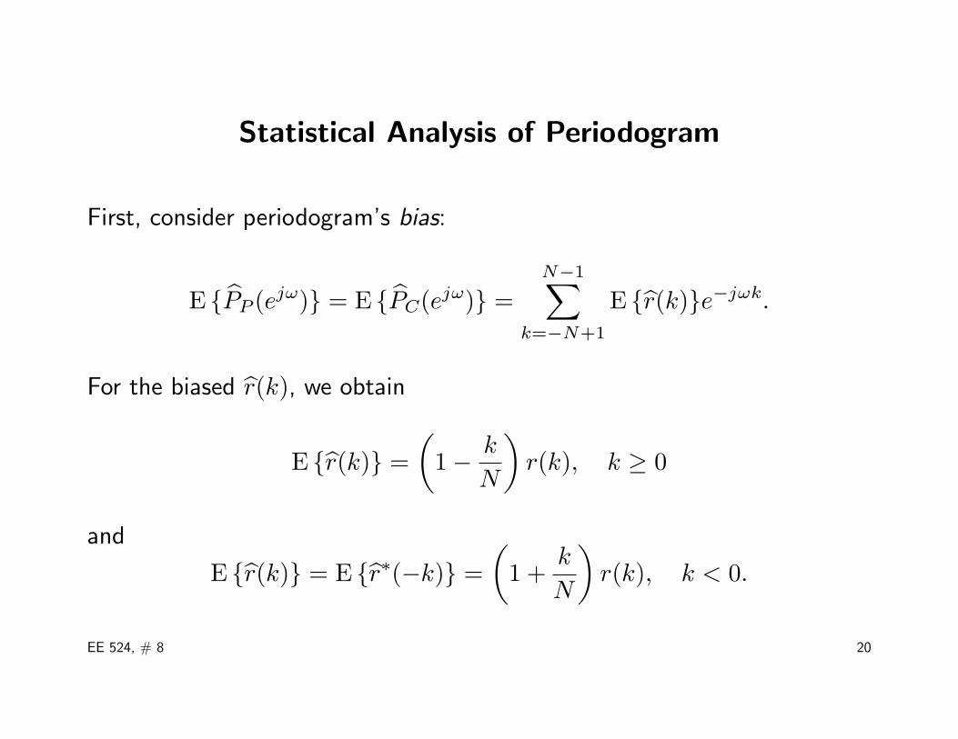
Statistical Analysis of Periodogram (cont.)
Remarks:
• Frequency resolution of periodogram is approximately equal to 1/N ,because the −3 dB mainlobe width WB in frequency f is ≈ 1/N .
• The mainlobe smears or smoothes the estimated spectrum,
• Sidelobes transfer power from the frequency bands that concentratemost of the power to bands that contain less or no power. This effect iscalled leakage.
EE 524, # 8 24

Statistical Analysis of Periodogram (cont.)
Now, consider periodogram variance.
Assumption: x(n) is zero-mean circular complex Gaussian white noise:
E {Re [x(n)]Re [x(k)]} =σ2
2δ(n− k),
E {Im [x(n)]Im [x(k)]} =σ2
2δ(n− k),
E {Re [x(n)]Im [x(k)]} = 0,
which is equivalent to
E {x(n)x∗(k)} = σ2δ(n− k),
E {x(n)x(k)} = 0.
EE 524, # 8 25

E {P̂P (ejω)} =N−1∑
k=−N+1
(1− |k|
N
)r(k)e−jωk
=N−1∑
k=−N+1
(1− |k|
N
)σ2δ(k)e−jωk
= σ2 = P (ejω).
For our zero-mean circular white x(n):
E {x(k)x∗(l)x(m)x∗(n)} = E {x(k)x∗(l)}E {x(m)x∗(n)}+E {x(k)x∗(n)}E {x(m)x∗(l)}
= σ4[δ(k − l)δ(m− n) + δ(k − n)δ(m− l)].
EE 524, # 8 26

E {P̂P (ejω1)P̂P (ejω2)}
= E
{1N
( N−1∑k=0
x(k)e−jω1k)( N−1∑
l=0
x∗(l)ejω1l)
︸ ︷︷ ︸P̂P (ejω1)
× 1N
( N−1∑m=0
x(m)e−jω2m)( N−1∑
n=0
x∗(n)ejω2n)
︸ ︷︷ ︸P̂P (ejω2)
}.
EE 524, # 8 27

E {P̂P (ejω1)P̂P (ejω2)} =1
N2
N−1∑k=0
N−1∑l=0
N−1∑m=0
N−1∑n=0
E {x(k)x∗(l)x(m)x∗(n)}e−jω1(k−l)e−jω2(m−n)
=σ4
N2
N−1∑k=0
N−1∑l=0
N−1∑m=0
N−1∑n=0
[δ(k − l)δ(m− n)
+ δ(k − n)δ(m− l)]e−jω1(k−l)e−jω2(m−n)
= σ4 +σ4
N2
N−1∑k=0
N−1∑l=0
e−j(ω1−ω2)(k−l)
= σ4 +σ4
N2
N−1∑k=0
e−j(ω1−ω2)kN−1∑l=0
ej(ω1−ω2)l
= σ4 +σ4
N2
[1− e−jN(ω1−ω2)
1− e−j(ω1−ω2)
][1− ejN(ω1−ω2)
1− ej(ω1−ω2)
]= σ4 +
σ4
N2
{sin[(ω1 − ω2)N/2]sin[(ω1 − ω2)/2]
}2
.EE 524, # 8 28

Statistical Analysis of Periodogram (cont.)
limN→∞
E {P̂P (ejω1)P̂P (ejω2)}=P (ejω1)P (ejω2) + P 2(ejω1)δ(ω1 − ω2) ⇒
limN→∞
E {[P̂P (ejω1)− P (ejω1)][P̂P (ejω2)− P (ejω2)]}
={
P 2(ejω1), ω1 = ω2,0, ω1 6= ω2.
The variance of periodogram cannot be reduced by taking longer observationinterval (N → ∞). Thus, periodogram is a poor estimate of the PSDP (ejω)!
EE 524, # 8 29

Refined Periodogram- and Correlogram-based Methods
Refined periodogram Bartlett’s method (8.2.4 in Hayes):
Based on dividing the original sequence into L = N/M nonoverlappingsequences of length M , computing periodogram for each subsequence, andaveraging the result:
P̂B(ejω) =1L
L∑l=1
P̂l(ejω), P̂l(ejω) =1M
∣∣∣∣∣M−1∑n=0
xl(n)e−jωn
∣∣∣∣∣2
.
EE 524, # 8 30

Further Refinements of periodogram (Welch’s method, 8.2.5 in Hayes):
Welch’s method refines the Bartlett’s periodogram by:
• using overlapping subsequences,
• windowing of each subsequence.
EE 524, # 8 31

Continue Matlab ExampleConvemtional Periodogram: A = 0.1, N = 10000
EE 524, # 8 32

Averaged Periodogram: A = 0.1, N = 10000,M = 1000
EE 524, # 8 33

Welch Periodogram: A = 0.1, N = 10000,M = 1000 with2/3 Overlap and Hamming Window
EE 524, # 8 34

Refined Correlogram(Blackman-Tukey method, 8.2.6 in Hayes):
• r̂(k) is a poor estimate of higher lags k. Hence, truncate it (use M � Npoints).
• Use some lag window:
P̂BT(ejω) =M−1∑
k=−M+1
w(k)r̂(k)e−jωk.
Hence
P̂BT(ejω) =12π
∫ π
=π
W (ej(ω−ν))P̂P(ej(ω−ν))dν,
i.e. frequency smoothing of the periodogram.
EE 524, # 8 35

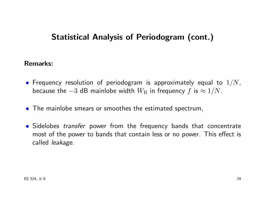
High-resolution Nonparametric Methods (8.3 in Hayes)
Consider FIR filter with the impulse responseh∗(0), . . . , h∗(N − 1) and the output is
y(k) =N−1∑n=0
h∗(n)x(k − n) = hHx(k).
The output power:
E {|y(k)|2} = E {|hHx(k)|2}= hHE {x(k)xH(k)}h= hHRh.
EE 524, # 8 36
Filter frequency response
H(ejω) =N−1∑n=0
h∗(n)e−jωn = hHa(ω),
where
a(ω) =
1
e−jω
...e−j(N−1)ω
.
EE 524, # 8 37

High-resolution Nonparametric Methods: Capon
The key idea of the Capon method: let us “steer” our filter towardsa particular frequency ω and try to reject the signals at all remainingfrequencies:
minh
E {|y(k)|2} subject to H(ejω) = 1 =⇒
minh
hHRh subject to hHa(ω) = 1.
Q(h) = hHRh + λ[1− hHa(ω)] + λ∗[1− a(ω)Hh] =⇒∇Q = Rh− λa(ω) = 0 =⇒ hopt = λR−1a(ω)
note similarity with the Yule-Walker equations!
EE 524, # 8 38

Substituting back into the constraint equation hHa(ω) = 1, we obtain
hHa(ω) = λ∗aH(ω)R−1a(ω) = 1 =⇒ λ =1
aH(ω)R−1a(ω).
Hence, the analytic solution is given by
hopt =1
aH(ω)R−1a(ω)R−1a(ω).
EE 524, # 8 39

High-resolution Nonparametric Methods: Capon (cont.)
PCAPON(ejω) = E {|y(k)|2}|h=hopt
= hHoptRhopt
=aH(ω)R−1RR−1a(ω)
[aH(ω)R−1a(ω)]2
=1
aH(ω)R−1a(ω).
This spectrum is still impractical because it includes the true covariancematrix R. Take its sample estimate
P̂CAPON(ejω) =1
aH(ω)R̂−1a(ω).
EE 524, # 8 40

AR Spectral EstimationIdea: Find the complex AR coefficients of the process and substitute themto the AR spectrum:
PAR =σ2
|A(ejω)|2=
σ2
|cHa(ω)|2
where c = [1, a1, . . . , aN−1]H. Recall that, according to the Yule-Walkerequations:
c = σ2R−1e1
where e1 = [1, 0, 0, . . . , 0]T . Hence, omitting σ2:
PAR(ω) =1
|aH(ω)R−1e1|2.
Maximum entropy spectral estimation: given covariance functionmeasured at N lags, extrapolate it out of the measurement interval by
EE 524, # 8 41

maximizing the entropy of the random process. Entropy of a Gaussianprocess can be written as (Burg):
H =12π
∫ π
−π
lnP (ejω)dω.
Burg’s method: maxH subject to
12π
∫ π
−π
P (ejω)ejωndω = r̂(n), n = 0, 1, . . . , N − 1.
This was shown to give the AR spectral estimate!
EE 524, # 8 42

Digression: Entropy
Let the sample space for a dicrete RV x be x1, . . . , xn. The entropy H(x)is proportional to
H(x) ∼ −n∑
i=1
p(xi) ln p(xi).
where p(xi) = Prob(x = xi): For continuous RV
H(x) ∼ −∫ ∞
−∞fx(x) ln fx(x)dx,
where fx(x) is the pdf of x.
EE 524, # 8 43