Embed Size (px)
Citation preview

Ann. Inst. Statist. Math. Vol. 56, No. 4, 611-630 (2004) Q2004 The Institute of Statistical Mathematics
SPECTRAL DENSITY ESTIMATION WITH AMPLITUDE MODULATION AND OUTLIER DETECTION*
JIANCHENG JlANG 1 AND Y. V. HUI 2
1LMAM and School of Mathematical Sciences, Peking University, Beijing 100871, China, e-mail: jiang~math.pku.edu.cn
2Department of Management Sciences, City University of Hong Kong, 83 Tat Chee Avenue, Kowloon, Hong Kong, China, e-mail: [email protected]
(Received October 31, 2002; revised October 14, 2003)
A b s t r a c t . This paper studies spectral density estimation based on amplitude mod- ulation including missing data as a specific case. A generalized periodogram is in- troduced and smoothed to give a consistent estimator of the spectral density by running local linear regression smoother. We explore the asymptotic properties of the proposed estimator and its application to t ime series data with periodic missing. A simple data-driven local bandwidth selection rule is proposed and an algorithm for computing the spectral density estimate is presented. The effectiveness of the proposed method is demonstrated using simulations. The application to outlier de- tection based on leave-one-out diagnostic is also considered. An illustrative example shows that the proposed diagnostic procedure succeeds in revealing outliers in time series without masking and smearing effects.
Key words and phrases: Amplitude modulation, local linear regression, missing ob- servations, outlier detection, spectral density.
1. Introduction
Let {Yt, t = 0, +1 , + 2 , . . . } be a s t a t i ona ry t ime series wi th m e a n zero and autoco- var iance funct ion R y ( v ) -- E[YtYt+v], v -- 0, +1 , i 2 , . . . . T h e n the p e r i o d o g r a m for the observed t ime series Yl, �9 �9 �9 Yn is given by
(1.1) i(n)(w) = ~ n t = l y t e x p ( - i t w ) 2 , w E [0,77].
I t is well-known tha t the pe r iodog ram is an a sympto t i ca l l y unbiased e s t ima to r of the spec t ra l densi ty funct ion
1 (3o
(1.2) f y ( w ) = ~ E R y ( t ) e x p ( - i t w ) , w E [0,771, t ~ - - o o
*Supported by Chinese NSF Grants 10001004 and 39930160, and Fellowship of City University of Hong Kong.
611

612 J IANCHENG JIANG AND Y. V. HUI
even though it is inconsistent. See for example Brillinger (1981), Priestley (1981) and Brockwell and Davis (1991). If {Yt} follows a stationary linear process, then the pe-
riodogam I(yn)(wk) at Fourier frequencies wk = 27rk/n (for k = 0 , 1 , . . . , N , where N = [ ( n - 1)/2]) are asymptotically independent. The asymptotic unbiasedness and independence of the periodogram allow one to construct a consistent estimator of fy (w) by locally averaging the periodogram. Most traditional methods are based on this ap- proach. See for example Brillinger (1981), Fan and Kreutzberger (1998), and others.
Other alternative estimators, such as the smoothed log-periodogram and Whittle likelihood-based estimator, have received much attention. Examples include: the au- tomatic smoothing of the log-periodogram in Wahba (1980); the penalized maximum likelihood spline estimator in Pawitan and O'Sullivan (1994); the logspline estimator in Kooperberg et al. (1995a, 1995b); and the local Whittle's likelihood estimator in Fan and Kreutzberger (1998). As demonstrated by Fan and Kreutzberger (1998), the Whittle likelihood-based estimators are desirable and outperform other estimators at regions where the log-spectral density is convex. Fan and Kreutzberger (1998) also recommend using Whittle's likelihood-based method.
However, our experience shows that there is little advantage of using Whittle's likeli- hood over the smoothed periodogram. One reason is that its asymptotic bias depends on the spectral density and the second derivative of log-spectral density, which complicates the choice of optimal bandwidth selector. Another reason is that the absolute value of the asymptotic bias of the Whittle-based estimator is larger than that of the smoothed periodogam in the region where fy(w) is convex, while the asymptotic variances are the same (see Remark 2 in Fan and Kreutzberger (1998) for bias comparison). Among these competitive approaches in spectral density estimation, both the smoothed peri- odogram and the Whittle likelihood-based estimator are asymptotically efficient. They also outperform the smoothed log-periodogram (see Fan and Kreutzberger (1998)).
When there are missing observations, direct use of the aforementioned methods is infeasible because the definition of periodogram in (1.1) is unclear. In addition, these approaches are nonrobust against outliers since they are based on least-squares or local maximum likelihood principles. Several authors have proposed regarding the missing observations or outliers as zeros, and then estimating the spectral density from the "ze- roed" data series. See for example Jones (1962), Parzen (1961, 1963), Priestley (1981), and Hui and Lee (1992) among others. A remarkable work in this field is that of Parzen (1963) in which amplitude modulation mechanics is proposed. We will employ Parzen's mechanics to develop a generalized periodogram and extend the smoothed periodogram of Fan and Kreutzberger (1998) in this study. The asymptotic normality of the proposed estimator of spectral density will be proven. The technical derivations of such asymp- totic property is very involved and determined efforts have been made. For robustness, one may smooth the logarithm of the generalized periodogram and then estimate the spectrum using an exponential transformation. The proposed approach can be adapted naturally to the smoothed log-periodogram.
As pointed out in Fan and Gijbels (1996), the spectral densities are usually very rough and the periodogram is highly heteroscedastic. Global bandwidth smoothing is usually unsatisfactory in revealing the complicated structure of the frequently changing spectral density. We will develop a simple data-driven local bandwidth selection method for our spectral density estimator, which facilitates the application in outlier detection.
Note that the presence of outliers can severely distort conventional spectral estima-

SPECTRAL DENSITY ESTIMATION 613
tors even though such outliers are not large relative to the scale of the observations (see Kleiner et al. (1979)). Outlier detection is vital to nonrobust spectral estimation and the existence of masking and smearing effects in time series further complicates the prob- lem. We study an outlier detection procedure by evaluating the smoothed periodogram based on the widely used leave-one-out diagnostics. Therefore the spectral density can be estimated using the proposed method after outliers are removed from the data.
This paper is organized as follows. Section 2 introduces the generalized periodogram and the spectral density estimator. Section 3 considers asymptotic properties of the generalized periodogram and the spectral density estimator. A data-driven bandwidth selection rule is proposed and an algorithm for calculating the spectral density estimate is presented in Section 4. A simulation study on the performance of the proposed estimator for incomplete series is discussed in Section 5. Section 6 studies the application to outlier detection and Section 7 gives our conclusion. Technical proofs are presented in the Appendix.
2. Estimation
2.1 Parzen's amplitude modulation mechanics Consider the amplitude modulation mechanics for spectral density estimation with
missing values in Parzen (1963). The time series we are interested in is {Yt}, but the observed series is {Xt}. The amplitude of time series {Yt} is modulated by {gt} through the relationship
( 2 . 1 ) = 9,Y ,
where {gt} is a non-random bounded series possessing a generalized harmonic analysis in the sense that for v : 0, 1 , . . . ,
1 n - - v
(2.2) Rg(v) lim E = -- gtgt+v n - - * o o n
t = l
exists. For a systematically unobservable series, such as a stock index which is unobserv- able on certain days in a year, it may be more appropriate to model this phenomenon as an amplitude modulated series with gt defined by
0 if Yt is missing at time t, (2.3) gt = 1 if Yt is observed at time t.
For a general missing pattern, (2.1) can also be used by letting Xt represent the observed value of Yt with 0 inserted in the series whenever the value of Yt is missing.
2.2 Generalized periodogram Suppose {Xt} is asymptotically stationary, i.e. Rx(v) -- limn-.ccl/n~-~.tn-1 v
E[XtXt+v] exists. Then (2.1) leads to Rx(v) -- Rg(v)Ry(v). According to Parzen (1963), if {Yt} is an ergodic normal process, then {Xt} is ergodic. The sample auto- covariance function of {Zt}, Rx(v) = 1/n ~-]tn=-i v XtXt+v, is a consistent estimator of Rx(v) in the quadratic mean. Therefore, if Rg(v) r 0, then Ry(v) can be consistently estimated by
Rx(v) for v = 0,1, . . . . ( 2 . 4 ) '

614 JIANCHENG JIANG AND Y. V. HUI
For v -- - 1 , - 2 , . . . , let /~y(v) -- R y ( - v ) . This motivates us to define the following generalized periodogram.
DEFINITION 2.1. For the time series {Yt} with modulated amplitude, its general- ized periodogram is defined as
1 (2.5) GI(n)(wk) = - ~ E Ry(v)exp(- ivwk) ,
rvl<n
where wk = ~-~ (k = 0, 1 , . . . , N) are Fourier frequencies.
The generalized periodogram has properties similar to the common periodograms. It can be used to construct a variety of tests for hidden periodicities following the ideas of common tests based on the periodogram in (1.1). The generalized periodogram has the following asymptotic representation for the bias and covariances.
PROPOSITION 2.1. I f { Yt } is ergodic and normal with mean zero, then the following results hold for k = 1 , . . . , N
(1) Asymptotic unbiasedness: E[aI(y~)(wk)] = fy(wk) + 0 ( - ~ ) .
(2) Variance approximation: Var[GI(")(Wk)] = f~(wk) + T~(Wk) + O(1). (3) Asymptotic independence: for wj r Wk,
Cov(Gl(yn)(wj), Gl(~)(Wk)) = O ( 1 ) .
A detailed proof of Proposition 2.1 is given in the Appendix and T~ (w) is defined in Theorem 3.1.
2.3 Local linear regression smoother Note that the generalized periodogram is an asymptotically unbiased estimator of
fy(w) at Fourier frequencies. However, it is inconsistent in estimating fw(w). A con- sistent estimator of fy(w), for w E [0, ~r], can be obtained via directly smoothing the
data {(wk, GI (n) (wk)), k = 1 , . . . , N} using a locally weighted average. Following Fan and Kreutzberger (1998), we run the local linear regression smoother to the data, and obtain the estimator
N
k-~l
where KN(t) ---- 1 SN._.._A~2 - ____-- ht" sN,1
Nh SN,O " SN,2 -----SY~ K(t) , N,1
where K(t) is a kernel funct ion and SN,s : N ~ Ek=IN K(W-._~_~)(~3n , , - OJk) t"
Other estimation approaches such as Whittle 's likelihood in Fan and Kreutzberger (1998), may be indiscriminately applied, but we will not pursue these options further
in this paper. Furthermore, the distribution of GI(y'~)(wk) is unknown under a general amplitude modulation or missing mechanism. It is unclear whether Whitt le 's likelihood principle applies in these situations.

S P E C T R A L D E N S I T Y E S T I M A T I O N 6 1 5
3. Asymptotic properties
In this section, we only consider the impor tant case where gt is a function with period 0 and Yt is a moving average process given by
oo
(3.1) Yt = E r Z, iLd Af(0,0-2). j ~ --OO
Assume that ~-~j ICjlj 2 < c~. The spectral densi ty of {Yt} is
0 -2 _ .
fy(w) = ~-~l~(e *~)l 2,
where V(e = Ej=- j exp(-ij ). It follows that the spectral density has a bounded second derivative. From Parzen ((1963), pp. 388-389), gt admits a harmonic representat ion
o (3.2) gt= E ekexp(itAk)Gk,
k = - @
)~ 21vk e r ~ 1 0 . where k = --~-, -- iS J, Gk 1 = Y ~-]~s=l exp(--~sAk)gs for k = O, i l , . . . , • and ek -= 1 for all k except tha t e+o -- ~ if 0 is even. Furthermore,
0
(3.3) Rg(v)= E eke_kGkG-kexp(--ivAk). k = - O
W h e n gt is not a periodic function and n is modera te ly large, one can use the approximat ion
n - - v
(3 .4 ) R (v) - n
t = l
The following assumptions and notat ions are needed to derive the asympto t ic prop- erties of the proposed estimator:
(i) {Yt} is a s ta t ionary and normal process with ~-~j ICily 2 < c~. (ii) The spectral density function f y (w) is positive on [0, ~].
(iii) The kernel function K(x) is a symmetr ic probabi l i ty densi ty function and has a compact support , [ -1 ,1] say. Let # 2 ( K ) = f l 1 u2K(u)du and Vo(K) = f l 1K2(u)du.
(iv) h --+ 0 and Nh -+ cc as n --+ oc. (v) The bounded ampli tude modula ted series {gt} with period 0 satisfies p =
1 n - v min v Rg(v) > 0 and ~ ~-~-t=l gtgt+v = Rg(v) + O(~n), uniformly in v.
Condit ions (i)-(iv) are derived from Fan and Kreutzberger (1998). For function gt 1 0 with period 0, Rg(v) -- -~ ~ t=l gtgt+v (see (2.4) in Parzen (1963)) and condit ion (v)
follows. An example where these condit ions hold is Parzen 's periodic missing pa t t e rn (see Parzen (1963), pp. 385-386).
THEOREM 3.1. Suppose assumptions ( i)-(v) hold. For each w E (0, ~r), we have
L L ]

616 JIANCHENG JIANG AND Y. V. HUI
For a boundary point w* = eh, we have
fv(wn) - fu(wn) - h2f~(O+)p2(K,c)
Af(O, vo(K, c)Tr[fy2 (0+) + T~(0+)]),
where
and
with
and
8 2 # 2 ( K , c ) ---- 2,c - 81,c83,c
2 , 8 0 , c 8 2 , c - 81, c
Vo (K, c) =
+ o(h2)]
f~-x (S2,c - Sl,ct)2K2(t)dt
= Y] eke lH , l /Y( + + k # l
SO,cS2, c 2 2 ' - - 81,c)
0 0 1
Hk,t ---- E eiWiG~-kG-~-l , Wj = ~ E exp(-is)~j)/Rg(s), i = - O s= l
f sj,c -- tJK(t)dt. 1
Theorem 3.1 gives the asymptotic distribution of the spectral density estimator. A detailed proof is given in the Appendix.
Remark 3.1. It is worth noting that the estimated spectral density inherits the boundary adaptation as discussed in Fan and Kreutzberger (1998). The estimator achieves the same convergence rate at the boundary as at the interior points. When gt = 1, i.e. Yt is always observed, we have T2(w) = 0. Our result coincides with the result in Remark 2 of Fan and Kreutzberger (1998). (Note that the convergence rate
in Fan and Kreutzberger (1998) is a typo.) Therefore, our result can be regarded as an extension of Fan and Kreutzberger (1998).
Remark 3.2. From Theorem 3.1, the asymptotic mean squared errors (MSE) for estimating f v (w) at w E (0, 7r) can be defined as
1 2 (3.5) MSE(h,w) = l h4[f~(w)p2(K)]2 + -~-~vo(K)Tr[fy(w) + ~-~(w)].
Therefore, the optimal local bandwidth for estimating f y (w) in the sense of minimizing MSE(h, w), is
(3.6) hopt(02) = N_I/5 (vo(K)Tr[f2(w) +_7~(w)]~ 1/5 \ [f~(w)#2(K)] 2 ] "
4. Data-driven local bandwidth selection
Identifying peaks of spectral density is of special interest since information on energy and period are carried by the peaks. The global optimal bandwidth works pretty well

S P E C T R A L DENSITY ESTIMATION 617
in the estimation of a generally smooth spectral density. However, the local bandwidth selector should be employed to capture the complicated structure (especially the peaks) of a changing spectral density.
For the nonparametric regression estimator (2.6), common global and local band- width choices developed in nonparametric regression literature can be applied. Examples include the "pre-asymptotic substitution method" of Fan and Gijbels (1995), the "plug-in bandwidth selection" in Ruppert et al. (1995), and the "empirical bias bandwidth selec- tor" of Ruppert (1997). However, these bandwidth selection methods usually involve a large computational burden for outlier detection. We present a simple rule for bandwidth selection which is easy to implement in practice.
From (A.n)-(A.7) in the Appendix, we know that the exact bias of fy(w) is
N
Bias(h,w) _~ E K N fY(COk) -- fY(CO), k = l
up to a negligible term of order Op(1/v/-~). We can evaluate Bias(h, w) and the asymp- totic variance in Theorem 3.1 for a given bandwidth h at co if we have a pilot estimate f y (co) for f y (co) in hand. We propose choosing the bandwidth minimizing the estimated mean squared errors
(4.1) MSE(h,w) = [Bias(h,w)] 2 + -~-fitvo(K)Tr[f~(co) + "?~(w)],
where Bia~s(h, co) and #2 (co) are defined as Bias(h, w) and ~_2 (co) respectively with f y (w) replaced by fy(w). Define
hopt (co) = arg min MS-'----E(h, w). h
A
Then we minimize the one-dimensional function MSE(h, cz) with respect to h at each fixed frequency w. hopt(W) can be evaluated at a grid of frequency points. The above bandwidth selection requires only a pilot estimate of the spectral density, which avoids estimation of higher order derivatives of the regression function in implementation of the "pre-asymptotic substitution" and "plug-in" methods. The proposed method is also sim- pler than the "empirical bias bandwidth selector" method proposed by Ruppert (1997), where the empirical bias is estimated by calculating the estimate of regression function rh(x, h) on a grid of bandwidth values and then modeling the behavior of rh(x, h) as h varies. Note that the asymptotic variance in (4.1) does not involve the variance of the white noise in (3.1). It follows that evaluation of the asymptotic variance is much eas- ier compared with the nonparametric regression case where the unknown error variance needs to be estimated from the data.
Common Newton's iterations can be applied to find t h e hopt(co) efficiently. We here synthesize the ideas in minimizing the asymptotic mean squared errors of the hazard rate estimator in Miiller and Wang (1994) and maximizing the local pseudo-likelihhod in Fan et al. (2003), and propose an algorithm to evaluate fy(w).
Algorithm for estimating fy(w) Step 1. Initial estimate of fy(w): Choose a kernel, such as the Epanechnikov ker-
nel, and an initial global bandwidth h0. The choice of the initial bandwidth depends

618 J IANCHENG JIANG AND Y. V. HUI
on the specific case. A possible value for h0 is } n -1/5, as recommended by Mfiller and Wang (1994), or the global optimal bandwidth estimate given in Fan and Kreutzberger (1998). The initial estimate fy(w) of fy(w) is obtained by employing h = h0 and (2.6). The pilot estimate of f r (w) may also be obtained via a parametric approach if one has a plausible parametric model in mind.
Step 2. Minimization of MSE(h, w): Choose an equispaced grid of m l points &i, i = 1 , . . . , r n l between 0 and 7r. For each grid point &i, compute MSE(h,&i) in (4.1) and obtain its minimizers tt(&i) on the interval, [ho/4, 10h0] say. The minimizers can be easily obtained using the estimate Tz(&k) as the initial value of minimization at the next grid point &k+l. The minimizer can be found within a few iterations.
Step 3. Bandwidth smoothing: Choose another equispaced grid of m2 points wr, r = 1 , . . . ,rn2, over the interval [0, 7r] on which the final spectral density estimate is desired. Running the following local linear smoother by employing the global bandwidth }to = h0 or 2h0:
m l
t, /
where Km, (t) is the local linear weight, similar to (2.6). The smoothed bandwidth is then used to estimate fy(wr).
Step 4. Final spectral density estimate: Obtain the estimate fy(wr) in (2.6) by employing the bandwidths h(w,-), for r = 1 , . . . , m2.
The bandwidth selector is not only easy to implement; the estimator is also stable in the peak regions where the bandwidths are smoothed by the local linear smoother in Step 3. This contrasts with the claim made by Fan and Gijbels ((1996), p. 242). The steps can be iterated using the estimate fy(wr) in Step 4 as initial estimate in Step 1 and repeating Steps 2-4. The proposed spectral density estimation method can be easily applied to time series analysis with missing observations.
5. Simulations
We conduct a simulation study to compare the performance of the proposed method under a periodic missing pattern with the complete observation case. Note that for the complete observation case the proposed estimator is just the smoothed periodogram in Fan and Kreutzberger (1998), but for the incomplete observation case the latter estimator is not directly applicable.
For simplicity, we chose the popular Epanechikov kernel
K ( x ) = o .75(1 - x )S(Ixl <<_ 1).
The data-driven local bandwidth selection rule in Section 4 was applied in the simula- tions. To compare the performance of different estimators in simulations, we use 'typical' dataset in the sense that, based on the dataset, the estimators have their median per- formance in terms of average squared deviation loss at grid points where the estimators are evaluated.
Consider the ARMA model
(5.1) Yt + alYt-1 + " - + apYt-p = et + blet-1 + bqet_q,

S P E C T R A L D E N S I T Y E S T I M A T I O N 619
where et ~ A/'(0, 1). The following two examples were studied in Wahba (1980) and Fan and Kreutzberger (1998).
Example 1. The AR(3) model with al = - 1 . 5 , a2 = 0.7 and a3 = - 0 . 1 and the rest of the coefficients equal to zero.
Example 2. The MA(4) model with bl = - 0 . 3 , b2 = - 0 . 6 , b3 -- - 0 . 3 and b4 = 0.6 and the rest of the coefficients equal to zero.
No missing and weekly missing patterns were considered for these examples. Here we specifically generated the missing pattern in each simulated series. We kept the simulated observations for five t ime points , then dropped the next two observations.
o~
Typical estimated periodogram and spectral density with complete data
I I I I I I ]
0 , 0 05 1.0 1.5 20 2.5 3,0
Typical estimated periodogram and spectral density with incomplete data
,J: i!;
t i E i ~ i ,
O 0 0,5 1.0 15 2.0 25 3 . 0
o_
9 -
o. ,
Confidence interval of spectral density with complete data
: i
0.0 0.5 1.0 1.5
Confidence interval of spectral density with incomplete data
\
o. :
o .
m ,
2.0 2.5 3,0 0.0 0,5 1,0 1.5 2.0 2.5 3.0
Fig. 1. Numerical results for Example 1.
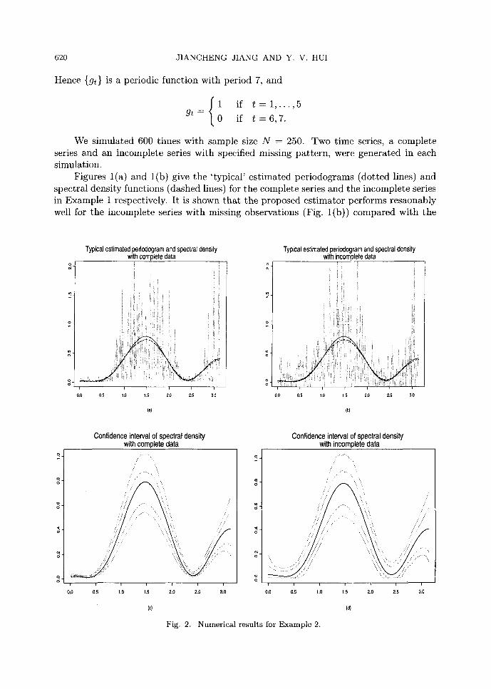
620 JIANCHENG JIANG AND Y. V. HUI
Hence {gt} is a periodic function with period 7, and
1 if t = 1 , . . . , 5 gt = 0 if t = 6, 7.
We simulated 600 times with sample size N = 250. Two time series, a complete series and an incomplete series with specified missing pattern, were generated in each simulation.
Figures l(a) and l(b) give the 'typical' estimated periodograms (dotted lines) and spectral density functions (dashed lines) for the complete series and the incomplete series in Example 1 respectively. It is shown that the proposed estimator performs resaonably well for the incomplete series with missing observations (Fig. l(b)) compared with the
Q C, -
Typical estimated periodogram and spectral density with complete data
~ii! i !
i r i i i i i i
oo 0.5 1.0 1,5 2.0 2.5 3.0
Confidence interval of spectral density with complete data
Typical estimated periodogram and spectral density with incomplete data
:~ i l i !i i;
ii i i i ~ ]i ii i li:i
:i:: :ii: :! :i:: : ' ! !i :~ :'i~iiiii" ~!!:;ii;:i ::
O 0 0 , 5 1 . 0 1 5 20 2.5 3 , 0
o".
i
/
D
I i i ~ i i
0 . 0 0.5 1.0 1.5 2 .0 2 .5 3 .0
Confidence interval of spectral density with incomplete data
O �9 . . ' , " . . , ,
/ - . . . . =
o
�9
o "
d
e4 o "
Q d . . . . . . . . . . . . . . . . . . . . . . . . . . . . . . . . . . . . . .
0.0 0 .5 1,0 1,5 2 .0 2 .5 3.0
Fig. 2. Numerical results for Example 2.

SPECTRAL DENSITY ESTIMATION 621
complete series (Fig. l(a)). The difference is insignificant. This demonstrates that the proposed estimator gives a good estimate under the missing observation situation. Fig- ures l(e) and l(d) also plot the envelopes (dotted lines) of the true spectral density (solid line) constructed from the pointwise sample percentiles. These envelopes repre- sent pointwise 2.5%, 12.5%, 87.5% and 97.5% sample percentiles of the spectral density estimates among 600 simulations. The estimated envelopes in Figs. 1(c) and l(d) in- dicate that the proposed method gives good confidence bounds for the spectral density function when there are missing obervations. Therefore it is insensitive to missing ob- servations. It also demonstrates that these confidence bounds provide a reliable tool in outlier detection, which is discussed further in the next section. Figure 2 plots the esti- mated spectral densities and envelopes for complete and incomplete series generated from Example 2. Results from Example 2 with a unimodal spectral density (Fig. 2) reconfirm the conclusion drawn from Example 1 with a J-shaped spectral density (Fig. 1).
It is shown for the above two examples that the proposed estimator performs reason- ably well with about 30% missing observations in comparison to the case where complete observations available. To assess the effectiveness of the proposed estimator for a higher proportion of missing, we considered the following weekly missing pat tern with a periodic function gt such that
1 if t = 1 , 3 , 5 , 7 gt = 0 if t = 2,4, 6.
There are about 43% missing observations. For the previous two examples, the perfor- mance of the proposed estimator under this missing pattern is similar to that under the previous pattern, but with a slightly wider confidence band. The results will not be displayed here due to space constraint.
Example 3. Continuation of Example 2 with random missing pattern. In this ex- ample, we use the following random missing pattern to illustrate how to use the proposed
Typical estimated periodogram and spectral density with random amplitude modulation
0.0 0,5 1+0 1.5 2.0 2.5 3,0
q _
o=..
Confidence interval of spectral density with random amplitude modulation
. . , / . . " . , . .
i i t t t i
0.0 0.5 1.0 1,5 2.~ 2.5 3.0
(b)
Fig. 3. Numerical results for Example 3.

622 JIANCHENG JIANG AND Y. V. HUI
estimation approach and to investigate if the method works in the setting:
P(gt = O lgt-1 = 0) = 0.3, P(gt = 0 I gt-1 = 1) = 0.2
with initial condition g0 = 1 (i.e. {gt} is a Markov chain). For the MA(4) model in Example 2, we simulated 600 samples for {Yt} with size N --- 250. For each sample, {gt} was sampled from the above Markov chain and {Xt} was the observed series. Because no optimal bandwidth is available for the proposed estimator in this case, we use the one for the spectral density estimation on {Y~} in our simulations.
Figures 3(a) and 3(b) show the typical estimated curve and the pointwise 2.5%, 12.5%, 87.5% and 97.5% sample percentiles of the proposed estimators among 600 sim- ulations for this example. Note that only {Xt} was observed, direct use of the common smoothed periodogram for {Xt} in Fan and Kreutzberger (1998) would result in a bi- ased estimator of the spectral density of {Yt}. Given {Xt} and the transition probability matrix of {9t}, we computed the proposed estimator. Figure 3 demonstrates that for the random missing pattern the proposed estimator truely captures the structure of the spec- tral density even though the bandwidths employed here are not optimal. Further s tudy on the optimal choice of bandwidth in this case requires derivation of the asymptotic bias and the asymptotic variance of the estimator, which is worthy of further investigation.
{5. Outl ier detection
The existence of outliers may affect model identification, which is essential in time series analysis. See for example Abraham and Chuang (1989), Bruce and Martin (1989), Subba Rao (1989), and Tsay et al. (2000) among others. Our suggested method only requires a nonparametric estimation of spectral density which avoids the identification problem. Thus, it is expected that the diagnostic based on nonparametric spectral estimation be more reliable than common diagnostics based on parametric models.
The welt-known masking and smearing phenomena post a difficult problem in the diagnostic tests for time series data. Earlier work in this area was presented in Chernick et al. (1982), Martin and Yohai (1986), and Bruce and Martin (1989). In spectral density estimation, outliers with a relatively large value compared with the scale of the innovation process will distort the estimator. These "outlying" points may not have a relatively large value compared with obervations' scale. We adopt the common leave-k-out diagnostic method to identify outliers in the spectral density estimation. The leave-k-out diagnostic has been widely used in regression analysis (see Cook and Weisberg (1982) and Atkinson (1985)). Bruce and Martin (1989) and Hui and Lee (1992) also studied the leave-one- out approach in the time series context. We expect that our diagnostic approach based on deletion and the proposed spectral density estimation identifies outliers (especially innovation outliers) without masking and smearing effects.
For illustration, we only consider the leave-one-out diagnostic method in outlier detection when there are missing observations. A multiple-deletion diagnostic can be developed in the same way, but we will not consider this problem since intensive com- putation would be required.
Diagnostic procedure for outlier detection (1) Confidence bound. Given a significance level a (1% or 5%, say), construct a
confidence bound for the spectral density with all available observations based on the

SPECTRAL DENSITY ESTIMATION 623
estimators in (2.6) and the normal approximation in Theorem 3.1:
1/2
f ly(W)- Bia~s(hopt(W),W)=k Zl_a/2 �9 (vo(K)Tr[f~(w) + r \ Nhopt(W) '
where Z1-~/2 is the 1 - ct/2 quantile of standard normal distribution. (2) Spectral density estmation with data deletion. Apply the leave-one-out approach
to estimate the spectral density. Evaluate the spectral density curves in (2.6) with the i-th observation deleted where observation i is regarded as periodic missing with period 0~- -n .
(3) Outlier identification. The i-th observation is identified as an outlier if the esti- mated spectral density curve with i-th observation deleted exceeds the confidence bounds in (1).
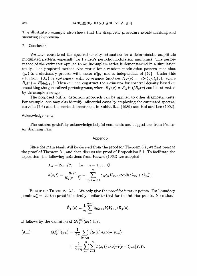
Example 4. Consider the yearly differenced RESEX series consisting of 77 obser- vations with two consecutive "outliers" at t = 71 and t = 72. The original RESEX dataset is given in Martin et al. (1983), and consists of Bell Canada inward movement of residential telephone extensions in a fixed geographic area from January 1966 to May 1973. As pointed out by Hui and Lee (1992), several common diagnostic approaches suffer from masking and smearing phenomena, which motivated Jiang et al. (1999) to use the robust Ll-norm fit of the dataset. Here we use the proposed diagnostic procedure to identify outliers in the data.
The data-driven bandwidth selection rule in Section 4 and the proposed diagnostic test were applied in this example. Figure 4(a) gives the estimated periodogram (solid line) and spectral density (dotted line), and Fig. 4(b) reports the 99% confidence bounds (dotted-dash lines) and the corresponding estimated spectral density curves with one observation in the dataset deleted as missing. It is shown that only the estimated curves with observations 71 and 72 deleted respectively stretch out of the confidence bounds. The two observations t --- 71 and t = 72 are correctly identified as outliers.
Estimated Period0gram and spectral density
o~
o -
0.0
i i i , , i
0.5 1.0 1.5 2.0 2.5 3.0
Confidence interval and estimated spectral densities ~ with deletion
~1".
o q
0 .0 0.5 1.0 1.5 2.0 2.5 3.0
(a) (b)
Fig. 4. Numerical results for Example 4.
624 J I A N C H E N G J I A N G A N D Y. V. H U I
The illustrative example also shows that the diagnostic procedure avoids masking and smearing phenomena.
7. Conclusion
We have considered the spectral density estimation for a deterministic amplitude modulated pattern, especially for Parzen's periodic modulation mechanics. The perfor- mance of the estimator applied to an incomplete series is demonstrated in a simulation study. The proposed method also works for a random modulation pat tern such that {gt} is a stationary process with mean E[gt] and is independent of {I/t}. Under this situation, {Xt} is stationary with covariance function Rx(v) = Ry(v)Rg(v), where Rg(v) = E[gtgt+v]. Then one can construct the estimator for spectral density based on smoothing the generalized periodograms, where Ry (v) -- Rx (v)/Ra (v) can be estimated by its sample average.
The proposed outlier detection approach can be applied to other diagnostic tests. For example, one may also identify influential cases by employing the estimated spectral curve in (2.6) and the methods mentioned in Subba Rao (1989) and Hui and Lee (1992).
Acknowledgements
The authors gratefully acknowledge helpful comments and suggestions from Profes- sor Jianqing Fan.
Appendix
Since the main result will be derived from the proof for Theorem 3.1, we first present the proof of Theorem 3.1 and then discuss the proof of Proposition 2.1. To facilitate the exposition, the following notations from Parzen (1963) are adopted:
Am=21rm/O, for m = 1 , . . . , O O
g s g t _
h(s, t) - Rg(s - t) E emenHm,n exp[i(SAm + tan)]. m~n=--O
PROOF OF THEOREM 3.1. We only give the proof for interior points. For boundary points w* = ch, the proof is basically similar to that for the interior points. Note that
1
_Oy(v) = n t = l
It follows by the definition of GI(y '0 (wk) that
(A.1) 1
= E y(v)exp(-/wk) Iv]<n
n n 1
- 27rn E E h ( s , t ) exp[ - i ( s - t)wk]YsYt. 8=1 t = l
S P E C T R A L D E N S I T Y ESTIMATION 625
Denote the discrete Fourier transforms of {Yt} by fig(w) - 1 }-~n exp(-isw)Ys. 2 x / ~ s = l
Then aI(y n) (~) can be rewritten as
e (A.2) GI(n)(w)_ 1
27rn E em en Hrn,n
x ~ exp[i(sAm + tan)] exp[- i ( s - t)w]Y, Yt s,t=l
e n
= E ernenHmn, ~o/5-'~-~1 E exp[_ i s ( co_Am)]ys m,nm--~ v ~Ji1~ s = l
1 ~ exp[it(w + An)]Y t • ~ t = l
O
- ~ ~ n H m , J ~ ( ~ - A~)J~(~ + An) m,n=--O
From the proof of Theorem 10.3.1 in Brockwell and Davis (1991) , we have
(A.3) Jg(w) : 9(e-{~)Jz(w) + rn(w),
where Yn(W) -- 1 0o "" 2,/Y~ Y~J=-~r such that ElYn(W)[ 4 = O(n -2) and Unj = n--j Zse_is w n Zse_isw. ~-~s=l-j - - ~-~s=l Combining (A.2) and (A.3) gives
GI(n)(w) = e
E emenHm,nlUUUUUW(e-i(c~ -- Am)qd(e-i(~~ + An)
ernenHm,n[k~(e-i(~~ - Arn)Yn(cO q- An)
+ rn(~ - Am)V(e-*(~+~~ + An)
+ rn(~ - Am)Yn(~ + An)]~ )
-- Anl (w) + An2 (w).
Therefore
N N ( ) (1.4) ]y(w) --- E KN Anl(Wk) + E KN W --Wk k=l k----1 -~ An2(aJk)
-= Mn(~) + Rn(~).
Observe that max~c[0,~ ] ElYn(co)l 4 = O(n-2) , so we have An2(W) = Op(-~) uniformly
in w E [0,7r]. Hence Rn(w) = O p ( ~ ) , which is an asymptotically negligible term, and
suffices to derive the asymptotic distribution of Mn (w).

626 JIANCHENG JIANG AND Y. V. HUI
Note that
n 1 Anj(W)-- E 2~n
s,t=l
n
=- E r~(s,t)Z~Zt. s,t=l
Z~Zt
Observing Hm,n = H - n , - m , we have rw(s, t) = r~(t, s). Then Anl(W) is real. Therefore by (A.4),
(A.5) k=l s,t=l
---- s~l k=l rwk
+ ~ KN ~ r~(8,t) z~z, l<s~=t<_n [.k=l
-= Bnl(~) + B~2(~).
We show that Bnl(W) contributes to the bias, and Bn2(w) to the variance of M,~(w). Direct calculation gives
and
N E[Snl(O..))] : E K N ( O d - W k ) k=l -h fy(wk)
= fy(~) + lh2f~(~)~2(K) + o(h2),
Var[Bnl(02)] = f i KN ~ h O')k rwk(8,8)
:o(1) 2or 4
Then
(A.6) Bnl (W) -- fy(w) + ~h2 f~(w)tL2(K) + o(h 2) -~-Op I--~n I .
It remains to show that
(A.7) W(n) = x/-NhBn2(w) ~ Af(0, vo(K)Tr[f2(w) + T~(W)]).
S P E C T R A L DENSITY ESTIMATION 627
Note that
W ( n ) =
l~_s#t<_n
bs,t(w)ZsZt.
Zs Zt
Observe that b~,t(w) = bt,~(w) for s # t, hence it follows that a~,t(w) - [b~,t(w)+bt,~(w)]/2 is real. Then
(A.8) W(n) = + l ~ s < t ~ _ n
~- f i as,t(w)ZsZt, s , t = l
where a~,s(w) = 0 for s : 1 , . . . , n. Let A(w) = (as,t(w)) be n • n matrix, then A(w) is symmetr ic with vanishing diagonal elements. Applying Theorem 5.2 in de Jong (1987) to (A.8), one gets (A.7). This completes the proof of the theorem. De Jong 's Theorem is s ta ted in the following.
THEOREM A.1. Let Q(n) = E l < _ i # j < _ n aijZiZj be a quadratic form in independent random variables Zi (EZi = O, EZ~ = 1), with v l , . . . , V n the eigenvalues of the sym- metric matrix (aij), with vanishing diagonal elements: aii -- 0 for all i. Suppose there exists a sequence of real numbers c(n) such that (let a(n) 2 be the variance of Q(n)):
1) c4(n)a(n) -2 m a x l < i < n El~_j~n a? .~,3 --+ O, as n --~ c~; and 2) maxl<i<n E[Z~I(IZ~ I > c(n))] --~ 0, as n -~ c~. 3) / f the eigenvalues of the matrix (aij) are negligible: a(n) -2 maxl<~<n ,2 __~ 0, as
n ~ oo then a(n)_lQ(n) d N(O, 1), n ~ oo.
To apply the theorem, we need to check the following conditions: (1) A(w) is symmetr ic and has vanishing diagonal elements; (2) a (n ) 2 -- Var[W(n)] -- vo(K)7~[f2(w) + T~(w)] + 0(1); (3) there exists a sequence of real numbers e(n) --~ oo such tha t
c4(n)a(n) -2 max ~ a? .(w) --~ 0, as n--~ oc; l < i < n ~,3
l ~_j~_n
(4) m a x l < i < n E[Z2I(IZil > c (n ) ) ] ---* 0, as n --+ oo; and (5) a (n) -2 maxl<~<n p2 __~ 0, as n ~ ~ , where pi 's are the eigenvalues of the
matr ix A(w). Condit ions (1) and (4) are obvious from the definition of W(n) and the normali ty
of Z~ if there exists a sequence of real numbers c(n) ~ c~ in condi t ion (3). Note tha t
n n
max p2 <_ E # 2 __ n - l t r ( A 2 ( w ) ) = n - 1 E a2, t(w)" l < i < n
i=1 s , t = l

628 J IANCHENG JIANG AND Y. V. HUI
It follows that condition (5) holds if n -1 E~,t=l a2~,t(w) ~ O. Let
and
~m,~(~) = ~ ( e - ' ( ~ - ~ ) ) ~ ( e -~(~+~))
d2m,n(A; s, t) ---- e-iS()~-~m)e-it()~+~) + e-it()~-;~'~)e-isO~+~).
Then O
1 r~(s,t) = 2n~r E emenHm'~gm,n(A)e-i~(:~-;~m)e-it(~+~)"
m~n~--O
From the definition of as,t(w), direct computation leads to
as,t(w) -- 2 KN h [r~ (s, t) + r ~ k=l
2 E emengm,n_~_~7~EK N W--Wk m,n=--O k=l -h
(7_ 2 ~ 0 E
m,n=--O
(72 emenHm,n-~-~Tr ~m,n (~)d2m,n (W;
\ - - ) ~,~,,~(~k)r ~, t)
s, t)(1 + O(h~)),
uniformly for s, t with s ~ t. T h e n E t= ln a~,t(w ) = O(h) uniformly for s -- 1 , . . . , n. Hence
max E a~,t(w) ~ 0 and n -1 a~,t(aJ ) --* O. l < s < n t= l s,t=l
Conditions (3) and (5) hold if we take h --~ 0 and c(n) --* co. Condition (2) holds from the results of (A.4)-(A.7) and Lemma A.1 below. []
LEMMA A.1. Under assumptions (i)-(v), we have for each w E (0,~)
Var[Mn(w)] = ~---~vo(K)rr[f2(w) + ~-~(w)](1 + o(1)).
PROOF. Note that n
A~l(W) = ~ r~(s, t)Z~Zt. s,t= l
Following the same argument as that given in Parzen ((1963), equation 3.29), we have
(A.9)
and
(A.10)

SPECTRAL DENSITY ESTIMATION 629
uniformly in k, k'. Then
(A.11) N
Var[Mn(w)] = E K~v (w ~wa)Var[Anl(wk)] k=l
• C o v ( A n l (Wk), An2(Cak'))
---- Dnl + Dn2.
By (A.9), (A.10) and (A.11), simple algebra leads to
and
1 f2 Dnl -- ~--~Trv0(K)[ y(W) 4- T2(w)](1 -t- o(1))
which completes the proof the lemma. []
PROOF OF PROPOSITION 2.1. The proof is similar to the proof of Lemma A.1, and is shown by employing the arguments for (3.2), (3.3) and (3.29) in Parzen (1963). []
REFERENCES
Abraham, B. and Chuang, A. (1989). Outlier detection and time series modeling, Technometrics, 31, 241-248.
Atkinson, A. C. (1985). Plots, Transformations, and Regression: An Introduction to Graphical Methods of Diagnostic Regression Analysis, Clarendon Press, Oxford.
Brillinger, D. R. (1981). Time Series Analysis: Data Analysis and Theory, Holt, Rinehart & Winston, New York.
Brockwell, P. J. and Davis, R. A. (1991). Time Series: Theory and Methods, 2nd ed., Springer-Verlag, New York.
Bruce, A. G. and Martin, R. D. (1989). Leave-k-out diagnostics for time series, Journal of the Royal Statistical Society, Series B, 51,363-424.
Chernick, M. R., Downing, D. J. and Pike, D. H. (1982). Detecting outliers in time series data, Journal of the American Statistical Association, 77, 743-747.
Cook, R. D. and Weisberg, S. (1982). Residuals and Influence in Regression, Chapman 8z Hall, New York.
de Jong, P. (1987). A central limit theorem for generalized quadratic forms, Probability Theory and Related Fields, 75, 261-277.
Fan, J. and Gijbels, I. (1995). Data-driven bandwidth selection in local polynomial fitting: Variable bandwidth and spatial adaptation, Journal of the Royal Statistical Society, Series B, 57, 371-394.
Fan, J. and Gijbels, I. (1996). Local Polynomial Modelling and Its Applications, Chapman 8z Hall, New York.
Fan, J., Jiang, J., Zhang, C. M. and Zhou, Z. (2003). Time-dependent diffusion models for term structure dynamics, Statistiea Sinica, 13, 965-992.
Fan, J. and Kreutzberger, E. (1998). Automatic local smoothing for spectral density estimation, Scandinavian Journal of Statistics, 25, 359-369.
Hui, Y. V. and Lee, A. H. (1992). Assessing influence in time series, Communications in Statistics-- Theory and Methods, 21, 3463-3478.

630 JIANCHENG JIANG AND Y. V. HUI
Jiang, J., Hui, Y. V. and Zheng, Z. (1999). Robust goodness-of-fit tests for AR(p) models based on Ll-norm fitting, Science in China, 42, 337-346.
Jones, R. H. (1962). Spectral analysis with regularly missed observations, The Annals of Mathematical Statistics, 32, 455-461.
Kleiner, B., Martin, R. D. and Thomson, D. J. (1979). Robust estimation of power spectra (with discussion), Journal of the Royal Statistical Society, Series B, 41, 313-351.
Kooperberg, C., Stone, C. J. and Truong, Y. K. (1995a). Rate of convergence for logspline spectral density estimation, Journal of Time Series Analysis, 16, 389-401.
Kooperberg, C., Stone, C. J. and Truong, Y. K. (1995b). Logspline estimation of a possibly mixed spectral distribution, Journal of Time Series Analysis, 16, 359-388.
Martin, R. D., Samarov, A. and Vandaele, W. (1983). Robust methods for ARIMA models, Ap- plied Time Series Analysis of Economic Data (ed. A. Zellner), 153-169, US Bureau of Census, Washington D.C.
Martin, R. D. and Yohai, V. J. (1986). Influence functionals for time series, The Annals of Statistics, 14, 781-818.
Miiller, H. G. and Wang, J. L. (1994). Hazard rate estimation under random censoring with varying kernels and bandwidths, Biometrics, 50, 61-76.
Parzen, E. (1961). Mathematical considerations in the estimation of spectra, Technometrics, 3, 167-190. Parzen, E. (1963). On spectral analysis with missing observations and amplitude modulation, Sankhyd,
Series A, 25, 383-392. Pawitan, Y. and O'Sullivan, F. (1994). Nonparametric spectral density estimation using penalized
Whitt le likelihood, Journal of the American Statistical Association, 89, 600-610. Priestley, M. B. (1981). Spectral Analysis and Time Series, Academic Press, New York. Ruppert, D. (1997). Empirical bias bandwidths for local polynomial nonparametric regression and
density estimation, Journal of the American Statistical Association, 92, 1049-1062. Ruppert, D., Sheather, S. J. and Wand, M. P. (1995). An effective bandwidth selector for local least
squares regression, Journal of the American Statistical Association, 90, 1257-1270. Subba Rao, T. (1989). Discussion of the paper by Bruce and Martin, Journal of the Royal Statistical
Society, Series B, 41,313-351. Tsay, R. S., Pefia, D. and Pankratz, A. E. (2000). Outliers in multivariate time series, Biometrika, 87,
789-804. Wahba, G. (1980). Automatic smoothing of the log periodogram, Journal of the American Statistical
Association, 75, 122-132.