Embed Size (px)
Citation preview

Spectral Analysis ofPulse-Modulated rf Signals
ARL-TN-152 September 1999
William O. Coburn
Approved for public release; distribution unlimited.

The findings in this report are not to be construed as anofficial Department of the Army position unless sodesignated by other authorized documents.
Citation of manufacturer’s or trade names does notconstitute an official endorsement or approval of the usethereof.
Destroy this report when it is no longer needed. Do notreturn it to the originator.

ARL-TN-152 September 1999
Army Research LaboratoryAdelphi, MD 20783-1197
Spectral Analysis ofPulse-Modulated rf Signals
William O. Coburn Sensors and Electron Devices Directorate
Approved for public release; distribution unlimited.
The parameters that characterize a rectangular-shapedpulse-modulated sinusoidal signal are the carrier frequency, thepulsewidth, the repetition frequency, and the number of pulses in orthe duration of the signal. We use a Fourier series representation toshow the influence of these parameters on the spectrum of apulse-modulated signal at a microwave carrier frequency. When anadditional amplitude modulation is applied at audio frequencies, theresulting transient cannot be efficiently analyzed with numericaltransform techniques. We present approximate numerical andanalytical techniques to obtain the frequency spectrum of suchsignals. This approach allows the near-real-time spectral analysis ofmodulated signals. Thus, the resulting spectrum can be easilycalculated for idealized modulation waveforms. A typical example ispresented and the effect of pulse modulation on the spectral content
Abstract
of an rf signal burst is discussed.
ii
iii
Contents
1. Introduction ␣ ....................................................................................................................................... 1
2. Pulse-Modulated rf Signal ␣ .............................................................................................................. 32.1 Numerical Results ........................................................................................................................... 32.2 Calculated Results ........................................................................................................................... 6
3. Additional Modulation␣ .................................................................................................................... 8
4. Modulated rf Bursts␣ ........................................................................................................................ 11
5. Discussion␣ ........................................................................................................................................ 15
Distribution␣ ............................................................................................................................................ 17
Report Documentation Page␣ ................................................................................................................ 19
Table
1. Spectral characteristics of an rf burst of duration tmax and 1-W peak transmittedpower ................................................................................................................................................ 16
Figures
1. Single period of a rectangular pulse modulation waveform and single rectangularpulse FFT with 4 percent duty factor ............................................................................................. 4
2. Single pulse-modulated 1.3-GHz carrier FFT with 2 percent rf duty factor ............................ 63. Calculated spectrum of a pulsed rf signal at 1.3 GHz ................................................................. 74. Single period of a modulation waveform with 20 pulses, frequency-shifted FFT of
fundamental modulation, FFT of fundamental modulation showing spectral linecharacteristics, and FFT of fundamental modulation for T1 = 0.25 ms ..................................... 9
5. Single-pulse FFT in 2-ms time window scaled for 10 pulses ................................................... 106. Calculated fundamental spectrum scaled by duty factor ......................................................... 107. Modulation waveform for 50-pulse rf burst, scaled FFT result shifted to modulated
carrier, FFT result over 80-kHz span for comparison to 4(c), and FFT result over 20-kHzspan to show spectral line characteristics ................................................................................... 12
8. FFT result (times one-half) for two periods of modulation waveform and FFT resultfor truncation time window .......................................................................................................... 13
9. Energy spectrum by convolution of FFT results ........................................................................ 1310. Calculated energy spectrum for 10-ms rf burst signal .............................................................. 14

1
1. IntroductionA periodic time function f(t) with a period T0 can be represented as aninfinite sum of exponential functions. In particular, with an angularfrequency ω0 = 2π/T0 = 2π (frequency) υ0,
f(t) = α ne jnω 0tΣn= –∞
n=∞, (1)
is an exponential Fourier series expansion with coefficients
α n = 1
T 0f(t)e –jnω 0t
–T 0/2
T 0/2dt . (2)
The Fourier series is a valid representation when the Dirichlet conditionsare satisfied, which requires f(t) to be a finite periodic time function.1 Thetime function must be finite in the sense that it has a finite number ofmaxima, minima, and discontinuities in every finite interval.
For now, f(t) is considered an infinite-duration pulse train,
f(t) = f 0 t + nT 0Σ
n=–∞
n=∞, where f 0(t) =
f(t), t ≤ T 02
0, otherwise. (3)
Then the Fourier integral of f0(t),
F 0(ω) = f 0(t)e –jωt
–∞
∞dt = f(t)e – jωtdt
– T 0/2
T 0/2, (4)
is the continuous spectrum of one period of the signal f(t). A periodicrectangular pulse has an approximately band-limited spectrum, or F0(ω)<< F0(0) for |ω| < ωmax, where we take ωmax = 20π/T0. The Fouriertransform representation of the signal spectrum F(ω) is a sequence ofimpulses
F(ω) = 2πT 0
F 0 nω 0 δ ω – nω 0Σn=–∞
n=∞, (5)
defined by the spectral envelope, F0(ω). Then the Fourier series coeffi-cients are F0(ω)/T0, evaluated at ωn
= nω0 = 2πn/T0, or2
α n = 1T 0
F 0 (ω) nω 0. (6)
The band-limited representation includes the periodic extensions of thefundamental spectrum F0(ω) for all frequencies, which implies that f(t) isinfinite in duration. I relied on the band-limited approximation through-out to develop analytical and numerical PC tools to obtain the spectrumfor this class of signals. I used MATLAB® to calculate the band-limitedspectrum of periodic signals that modulate a single rf carrier at angularfrequency ωc = 2π fc. The physical rf signal is a burst of pulses and the
1Papoulis, A., The Fourier Integral and Its Applications, New York, NY: McGraw-Hill (1987).2Oppenheim, A. V., A. S. Willsky, and S. H. Nawab, Signals and Systems, 2nd ed, Upper Saddle River, NJ:Prentice Hall (1997).
2
sum in equation (3) would be truncated to 2N + 1 pulses. The pulse trainis truncated with a rectangular pulse window function in the time do-main (time-windowing) that corresponds to a frequency-domain convolu-tion.1
Consider a repetitive rectangular pulse-modulated rf carrier, where themodulating pulse is assumed to be ideal and has negligible rise- and fall-times compared to the width T. An additional amplitude modulation(AM) with the periodic function g(t) that has a period T2 ~ kT0 for integerk is often applied to the pulse-modulated rf signal. The fundamentalspectrum can be obtained from sampled transient data q0(tn) = f0(tn)g0(tn)over one period using numerical transform techniques such as the fastFourier transform (FFT). For low-frequency modulations (i.e., k >> 1), thisapproach quickly becomes numerically intensive if the high-frequencycarrier is included in the sampled transient. When all modulations have alow-frequency spectrum compared to the rf carrier, we need only sampleq0(t) sufficiently to resolve the highest frequency component of the modu-lation waveform. In this case, the MATLAB FFT routines can be used toefficiently obtain the spectrum for the modulation waveform, which isthen shifted to the single carrier frequency. I show that the rf modulationdetermines the spectral bandwidth (BW) of the modulated signal withimpulses at the rf pulse repetition frequency (PRF). Additional modula-tions reduce the peak amplitude according to the AM duty factor andintroduce impulses at the AM PRF. When only the spectral envelope is ofinterest, Q0(ω) can be directly calculated in the frequency domain (foridealized modulation waveforms) to approximate the modulated rfspectrum. Numerical and analytical approaches are compared and usedto investigate the effect of rectangular pulse modulation on the spectralcontent of a finite-duration rf burst.
1Papoulis, A., The Fourier Integral and Its Applications, New York, NY: McGraw-Hill (1987).
3
2. Pulse-Modulated rf SignalA rectangular pulse pX(t) symmetric about the time reference (t = 0) withunit amplitude and half pulsewidth X = T/2 has the frequency spectrum
P X(ω) =
2 sin ωT2
ω , (7)
with peak magnitude 2X = T and full bandwidth (FBW) 1/X = 2/T. Weuse this ideal pulse to modulate a microwave carrier where f0(t) = pX(t)c(t)= pX(t)cos(ωct) is a repetitive pulse-modulated sinusoidal signal. Thecarrier spectrum is a single frequency, as represented by C(ω) = 1/2{δ(ω +ωc) + δ(ω – ωc)}.
Then f(t) is a real, even function of time with Fourier coefficients
α n = 2T 0
f(t)cos nω 0t dt0
T 0/2. (8)
The partial sum fN(t) ~ f(t) is
f N(t) = α 0 + 2 α ncos (2πnt/T)Σ
n = 1
N, (9)
which can be written as an average over one period of f(t) with the Fou-rier kernel kN(t) as a weighting function.1 That is, fN(t) can be made toapproximate f(t) to an arbitrary accuracy in the interval |t| < T0/2 bychoosing more sinusoids in the expansion. The Fourier series coefficientsfor f(t) are αn
= F0(nω0)/T0, where
F 0(ω) = 12
P X ω – ω c + P X ω + ω c . (10)
Compared to equation (9), the positive frequency component of thisfundamental spectrum has the same FBW but half the magnitude. Al-though this band-limited spectrum implies an infinite-duration signal,there is no ambiguity in considering a finite number of samples. How-ever, by truncating equation (1) to a finite number of terms, we alsotruncate the Fourier series representation of the signal spectrum in equa-tion (5). This reduces the resolution in the frequency domain so that caremust be taken to adequately sample the modulation waveforms.
2.1 Numerical Results
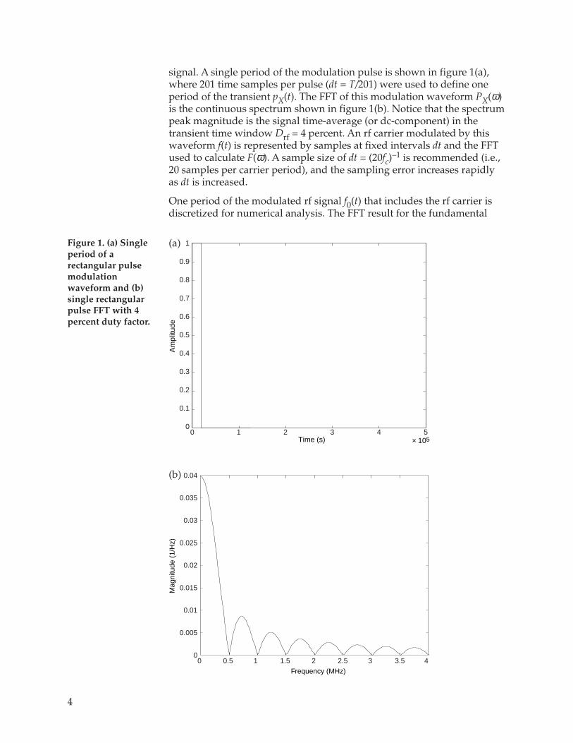
We consider a repetitive rectangular pulse modulation waveform pX(t)with constant pulsewidth (T) and PRF. The signal is periodic with periodT0 = 1/PRF and rf duty factor Drf = T/T0 in each period of the modula-tion. Since the periodic extensions of the fundamental spectrum are partof the FFT, the FFT result corresponds to an infinite rectangular pulsetrain. For example, let the carrier frequency be 1.3 GHz with T = 2 µs andT0 = 50 µs, assuming a unit amplitude (typically peak transmitted power)
1Papoulis, A., The Fourier Integral and Its Applications, New York, NY: McGraw-Hill (1987).
4
signal. A single period of the modulation pulse is shown in figure 1(a),where 201 time samples per pulse (dt = T/201) were used to define oneperiod of the transient pX(t). The FFT of this modulation waveform PX(ω)is the continuous spectrum shown in figure 1(b). Notice that the spectrumpeak magnitude is the signal time-average (or dc-component) in thetransient time window Drf = 4 percent. An rf carrier modulated by thiswaveform f(t) is represented by samples at fixed intervals dt and the FFTused to calculate F(ω). A sample size of dt = (20fc)
–1 is recommended (i.e.,20 samples per carrier period), and the sampling error increases rapidlyas dt is increased.
One period of the modulated rf signal f0(t) that includes the rf carrier isdiscretized for numerical analysis. The FFT result for the fundamental
Figure 1. (a) Singleperiod of arectangular pulsemodulationwaveform and (b)single rectangularpulse FFT with 4percent duty factor.
× 105Time (s)
Am
plitu
de
1
0.9
0.8
0.7
0.6
0.5
0.4
0.3
0.2
0.1
00 1 2 3 4 5
(a)
(b)
Mag
nitu
de (
1/H
z)
Frequency (MHz)
0.04
0.035
0.03
0.025
0.02
0.015
0.01
0.005
00 0.5 1 1.5 2 2.5 3 3.5 4
5
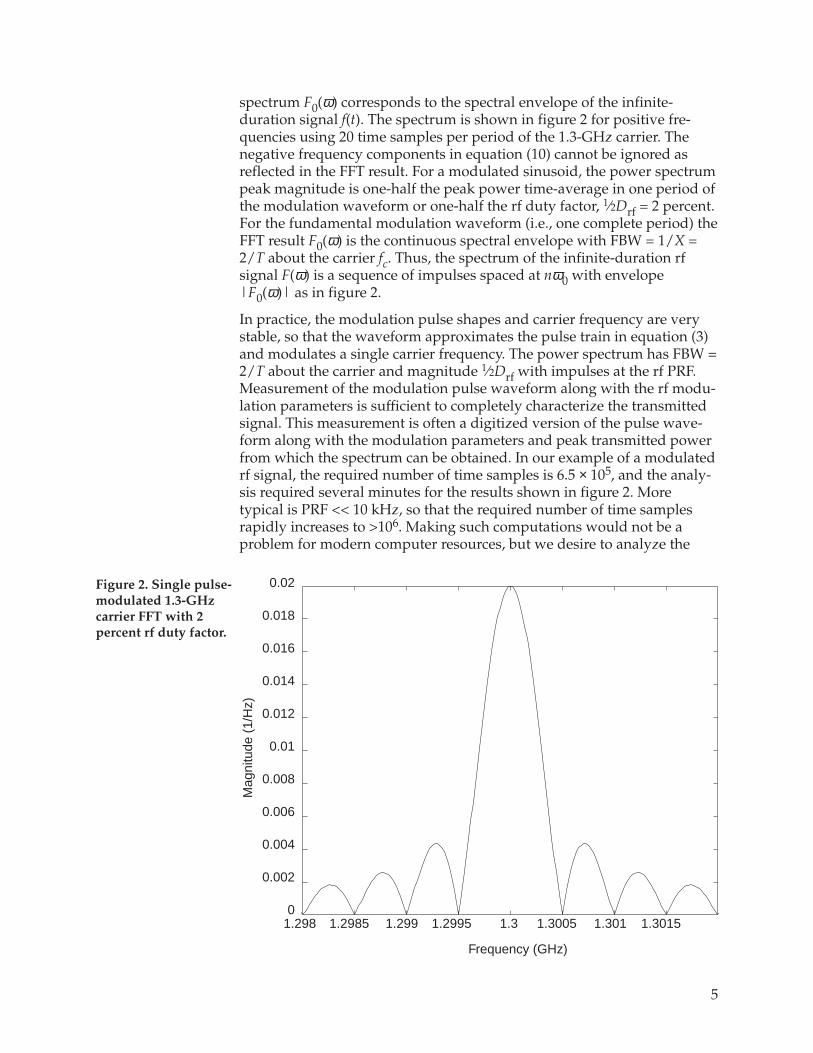
spectrum F0(ω) corresponds to the spectral envelope of the infinite-duration signal f(t). The spectrum is shown in figure 2 for positive fre-quencies using 20 time samples per period of the 1.3-GHz carrier. Thenegative frequency components in equation (10) cannot be ignored asreflected in the FFT result. For a modulated sinusoid, the power spectrumpeak magnitude is one-half the peak power time-average in one period ofthe modulation waveform or one-half the rf duty factor, 1⁄2Drf = 2 percent.For the fundamental modulation waveform (i.e., one complete period) theFFT result F0(ω) is the continuous spectral envelope with FBW = 1/X =2/T about the carrier fc. Thus, the spectrum of the infinite-duration rfsignal F(ω) is a sequence of impulses spaced at nω0 with envelope|F0(ω)| as in figure 2.
In practice, the modulation pulse shapes and carrier frequency are verystable, so that the waveform approximates the pulse train in equation (3)and modulates a single carrier frequency. The power spectrum has FBW =2/T about the carrier and magnitude 1⁄2Drf with impulses at the rf PRF.Measurement of the modulation pulse waveform along with the rf modu-lation parameters is sufficient to completely characterize the transmittedsignal. This measurement is often a digitized version of the pulse wave-form along with the modulation parameters and peak transmitted powerfrom which the spectrum can be obtained. In our example of a modulatedrf signal, the required number of time samples is 6.5 × 10⁵, and the analy-sis required several minutes for the results shown in figure 2. Moretypical is PRF << 10 kHz, so that the required number of time samplesrapidly increases to >106. Making such computations would not be aproblem for modern computer resources, but we desire to analyze the
Figure 2. Single pulse-modulated 1.3-GHzcarrier FFT with 2percent rf duty factor.
Frequency (GHz)
Mag
nitu
de (
1/H
z)
0.02
0.018
0.016
0.014
0.012
0.01
0.008
0.006
0.004
0.002
01.298 1.2985 1.299 1.2995 1.3 1.3005 1.301 1.3015
6
spectrum for more complex modulations in near real-time. As the timewindow required to include one full period of the modulated signalincreases, the number of time samples (with linear spacing) increasesrapidly. Numerical solution on a PC becomes time consuming; therefore,an analytical approach is desirable to obtain the pulse-modulated spec-trum for modulations that can be adequately represented by analyticfunctions.
2.2 Calculated Results
Fortunately, the modulations of interest have a frequency content that issignificantly lower than the carrier frequency. That is, the modulationwaveform pX(t) has a low-frequency spectrum PX(ω), where PX(ω) ~ 0 for|ω| < ωmax and ωmax
<< ωc. This implies that f(t) is an analytic functionof infinite duration, but even when it is truncated we still find that ωmax<< ωc with PX(ωmax) << PX(ωc), and the spectrum is approximately band-limited. The positive frequency components of the modulated signal are
F0 ω + =
P X ω – ω c
2T0=
sin X ω – ω c
T0 ω – ω c= Ac(ω)e jθc (ω) , (11)
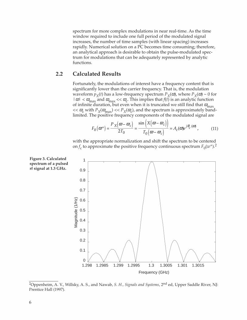
with the appropriate normalization and shift the spectrum to be centeredon fc to approximate the positive frequency continuous spectrum F0(w+).2
Figure 3. Calculatedspectrum of a pulsedrf signal at 1.3 GHz.
Frequency (GHz)
Mag
nitu
de (
1/H
z)
1
0.9
0.8
0.7
0.6
0.5
0.4
0.3
0.2
0.1
01.298 1.2985 1.299 1.2995 1.3 1.3005 1.301 1.3015
2Oppenheim, A. V., Willsky, A. S., and Nawab, S. H., Signals and Systems, 2nd ed, Upper Saddle River, NJ:Prentice Hall (1997).
7
Using the previous example modulation, 1⁄2PX(w) is shown in figure 3without amplitude correction, so the peak magnitude is X = T/2. As canbe seen from figure 2, the correct amplitude is obtained by normalizationto the time-average or dividing by tmax = T0. That is, the analytical resultis normalized to have the correct rf duty factor in one complete period ofthe modulation waveform to correspond to the FFT result. The completespectrum F(w) would have impulses at the PRF, but the fundamentalspectrum F0(w) is sufficient to characterize the spectral magnitude andFBW of the modulated signal. A convolution routine could also be used tocalculate F0(w) = PX(w) ƒ C(w)/4pT0 from the modulation and carrierspectra. In this manner, more complex carrier behavior could be included,but a single carrier frequency is sufficient in our analysis.
Thus, the spectrum for the infinite-duration pulse-modulated rf signalcan be readily approximated by FFT or direct calculation. For ideal rectan-gular pulse modulations, the transform is analytic but, in general, themodulation pulse is more complicated with only a digitized waveformrepresentation. We have shown that for low-frequency modulationscompared to a single carrier, the carrier frequency need not be resolved inthe sampled transient. Then measurement of one period of the repetitivemodulation waveform is sufficient to characterize the periodic signal.Then one can use numerical transform or analytical techniques to obtainthe fundamental signal spectrum, and we must realize that this representsthe envelope of the impulses contained in the actual spectrum. Develop-ing such tools is a first step in analyzing the spectrum as a function of themodulation parameters. Once obtained, the spectral content is useful inestimating the propagation, coupling, and scattering of modulated rfsignals.
8
3. Additional ModulationNow consider an additional rectangular pulse AM with pulsewidth T1and AM PRF = 1/T2. The composite signal is then q(t) = g(t)f(t) =g(t)pX(t)c(t), where g(t) = pX(t) is periodic with a period T2
~ kT0 forinteger k, and Y = T1/2. Since both g(t) and f(t) are even functions of time,so is q(t), with fundamental periods T0 and T2
~ kT0. The Fourier seriescoefficients for pY(t) are βn = PY(nω2)/T2, where ω2 = 2π/T2. The partialsum is
q N(t) = α mβ n – me
jnω 2tΣm= –M
MΣ
n=–N
N= γ ne
jnω 2tΣn=–N
N, (12)
where the sum over 2M + 1 terms is a convolution sum for the 2N + 1coefficients γn. Then
Q 0 nω 2 = γ nT 2 = T 2 α nβ n–mΣ
m=–M
m=+M, (13)
but this convolution is also numerically intensive. The convolution isequivalent to scaling the spectral amplitude in equation (11) because theadditional modulation changes the limits of integration in equation (4) tocorrespond to the fundamental period of the repetitive modulationwaveform. Thus the Fourier series coefficients for q(t) are weighted by thenew duty factor and
Q 0(ω) =T1 Ac (ω)
T2e jθc (ω) = DAM F0 (ω) (14)
is the Fourier transform of the fundamental signal q0(t). The spectrum forthe infinite-duration signal Q(ω) is a sequence of impulses at 1/T2 (and1/T0) with the envelope defined by equation (14). For idealized modula-tion waveforms, the spectrum PX(ω) can be obtained, normalized to thecorrect time-average, and scaled by one-half to account for the modulatedcarrier.
Consider a numerical approximation where the carrier frequency is notresolved and the FFT is used to obtain the spectrum of sampled tran-sients. Here we use at least 21 samples in the smallest pulse and linearspacing of the transient data for one complete period of the modulationwaveform. The rf carrier is 1.3 GHz, T = 2 µs, with rf PRF = 20 kHz, andwe apply an additional modulation characterized by the AM duty factorDAM
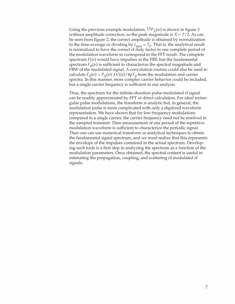
= T1/T2 and AM PRF = 1/T2. For example, let T1 = 0.5 ms and T2 =2␣ ms, so that the AM repetition frequency is 500 Hz and DAM = 0.25. Themodulation waveform contains 10 pulses as shown in figure 4(a) with theFFT in figure 4(b). The FFT result has been scaled by one-half to accountfor the modulated carrier and frequency-shifted to correspond to |Q0(ω)|for the modulated rf signal. In figure 4(c), I show an 80-kHz frequencyspan with dominant impulses at the PRF = 20 kHz, since now the FFTtime window includes repetitive pulses. The FBW of the spectral enve-lope depends on T (see fig. 4(b)) but the FBW of the impulses depends onT1, as can be seen in figure 4(c). The impulses appear at the PRF = 20 kHzand at 1/T1 = 2 kHz with FBW = 2/T1 = 4 kHz. Reducing T1 (while
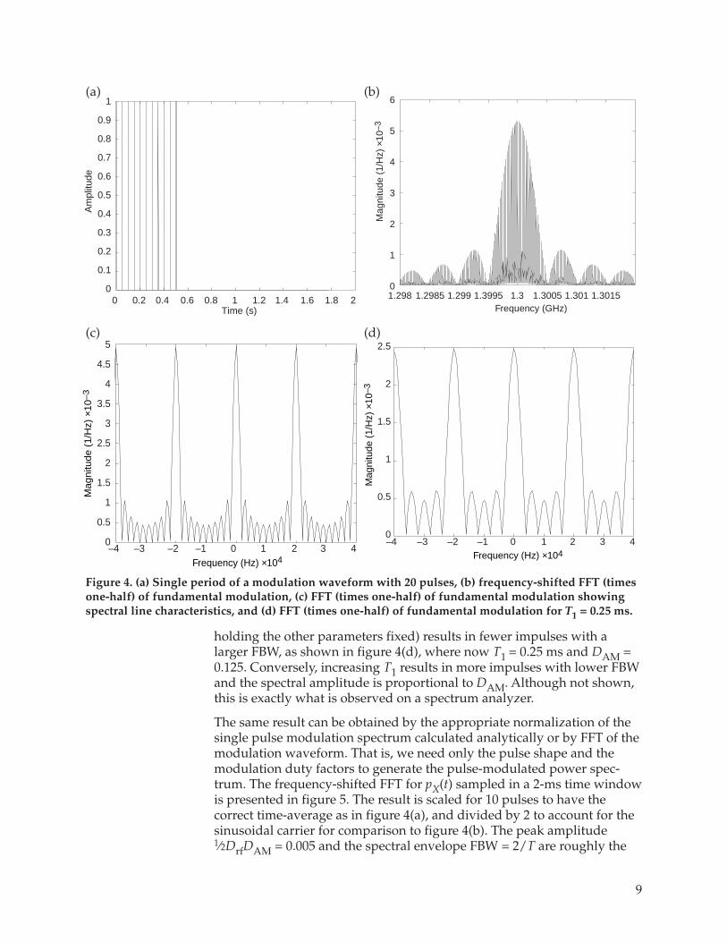
9
holding the other parameters fixed) results in fewer impulses with alarger FBW, as shown in figure 4(d), where now T1 = 0.25 ms and DAM =0.125. Conversely, increasing T1 results in more impulses with lower FBWand the spectral amplitude is proportional to DAM. Although not shown,this is exactly what is observed on a spectrum analyzer.
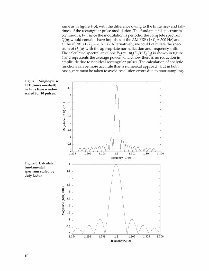
The same result can be obtained by the appropriate normalization of thesingle pulse modulation spectrum calculated analytically or by FFT of themodulation waveform. That is, we need only the pulse shape and themodulation duty factors to generate the pulse-modulated power spec-trum. The frequency-shifted FFT for pX(t) sampled in a 2-ms time windowis presented in figure 5. The result is scaled for 10 pulses to have thecorrect time-average as in figure 4(a), and divided by 2 to account for thesinusoidal carrier for comparison to figure 4(b). The peak amplitude1⁄2DrfDAM = 0.005 and the spectral envelope FBW = 2/T are roughly the
Figure 4. (a) Single period of a modulation waveform with 20 pulses, (b) frequency-shifted FFT (timesone-half) of fundamental modulation, (c) FFT (times one-half) of fundamental modulation showingspectral line characteristics, and (d) FFT (times one-half) of fundamental modulation for T1 = 0.25 ms.
Time (s)
Am
plitu
de1
0.9
0.8
0.7
0.6
0.5
0.4
0.3
0.2
0.1
00 0.2 0.4 0.6 0.8 1 1.2 1.4 1.6 1.8 2
Frequency (GHz)
Mag
nitu
de (
1/H
z) ×
10–3
1.298 1.2985 1.299 1.3995 1.3 1.3005 1.301 1.3015
6
5
4
3
2
1
0
Frequency (Hz) ×104
Ma
gn
itud
e (
1/H
z) ×
10
–3
5
4.5
4
3.5
3
2.5
2
1.5
1
0.5
0–4 –3 –2 –1 0 1 2 3 4
Frequency (Hz) ×104
Mag
nitu
de (
1/H
z) ×
10–3
2.5
2
1.5
1
0.5
0–4 –3 –2 –1 0 1 2 3 4
(a) (b)
(c) (d)
10
same as in figure 4(b), with the difference owing to the finite rise- and fall-times of the rectangular pulse modulation. The fundamental spectrum iscontinuous, but since the modulation is periodic, the complete spectrumQ(ω) would contain sharp impulses at the AM PRF (1/T2 = 500 Hz) andat the rf PRF (1/T0 = 20 kHz). Alternatively, we could calculate the spec-trum of Q0(ω) with the appropriate normalization and frequency shift.The calculated spectral envelope PX(ω − ωc)T1/(2T0T2) is shown in figure6 and represents the average power, where now there is no reduction inamplitude due to nonideal rectangular pulses. The calculation of analyticfunctions can be more accurate than a numerical approach, but in bothcases, care must be taken to avoid resolution errors due to poor sampling.
Figure 5. Single-pulseFFT (times one-half)in 2-ms time windowscaled for 10 pulses.
Mag
nitu
de (
1/H
z) ×
10–3
Frequency (GHz)
5
4.5
4
3.5
3
2.5
2
1.5
1
0.5
01.294 1.296 1.298 1.3 1.302 1.304 1.306
Figure 6. Calculatedfundamentalspectrum scaled byduty factor.
Mag
nitu
de (
1/H
z) ×
10–3
Frequency (GHz)
5
4.5
4
3.5
3
2.5
2
1.5
1
0.5
01.294 1.296 1.298 1.3 1.302 1.304 1.306

11
4. Modulated rf BurstsSince only a finite number of pulses are transmitted, the rf signal isactually a transient burst b(t) of a periodic waveform. For a whole numberof modulation periods, the duration does not change the modulation dutyfactor since the signal is repetitive, but it is needed to calculate the aver-age energy transmitted. We show this by windowing the periodic wave-form with a single rectangular pulse pZ(t) to truncate the pulse train at themaximum time tmax; so let Z = tmax/2.1 The spectrum PZ(ω) obtained bythe FFT has unit magnitude, since the time-average for this windowfunction is unity. The fundamental spectrum can be represented by aconvolution with the normalized PZ(ω), B0(ω) = PZ(ω) ⊗ Q0(ω)/2π, or
B0(ω) = sin (ωZ)4πωZ ⊗ Q0 (ω) . (15)
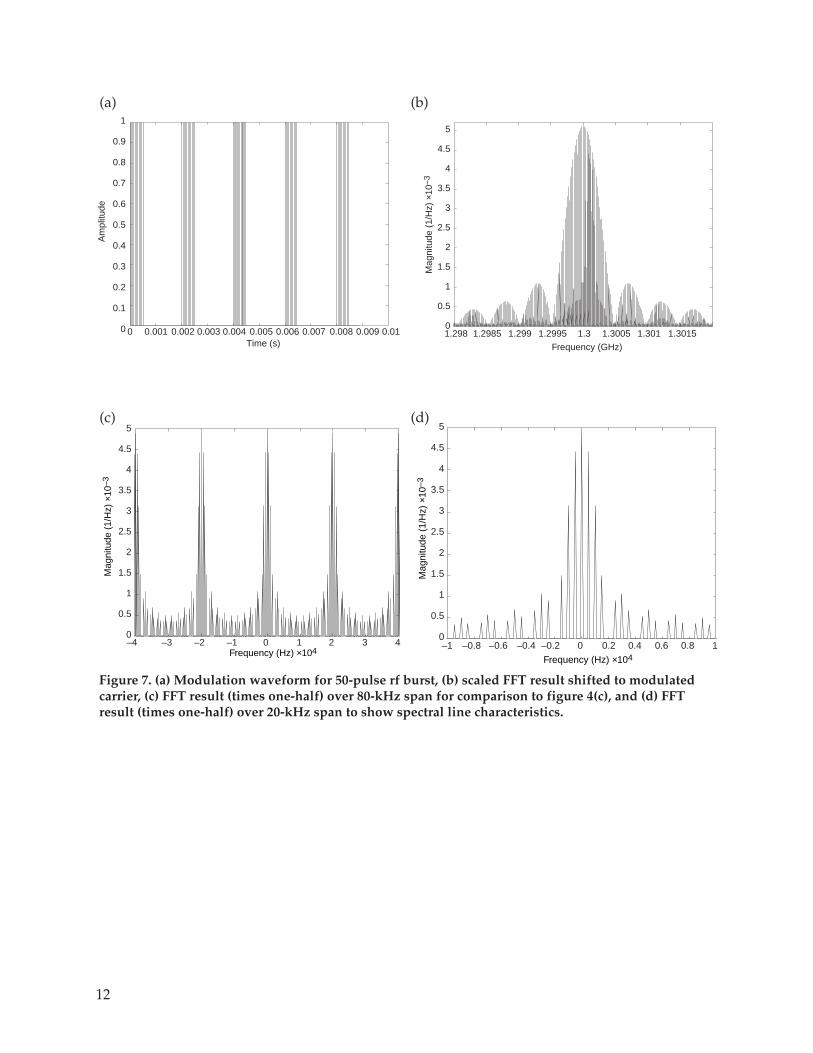
Thus, we could calculate the rf burst spectrum as a convolution of analyti-cal or FFT results and shift the result to ωc, but for measured data, FFTtechniques are often preferred for numerical efficiency. The modulationwaveform is shown in figure 7(a), truncated to tmax = 10 ms, which resultsin 50 rf pulses (or 5 AM pulses) with unit peak power transmitted. Thefrequency-shifted FFT result (scaled by one-half) for this example isshown in figure 7(b), and this is the power spectrum measured on aspectrum analyzer. The FFT result does not depend on the duration whenthe modulation duty factors are not modified (i.e., a whole number ofmodulation periods transmitted). In figure 7(c), we show an 80-kHzfrequency span for comparison to figure 4(c). The impulses in figure 4(c)represent another envelope of sharp impulses at the lowest PRF (500 Hzin this example) as shown in figure 7(d).
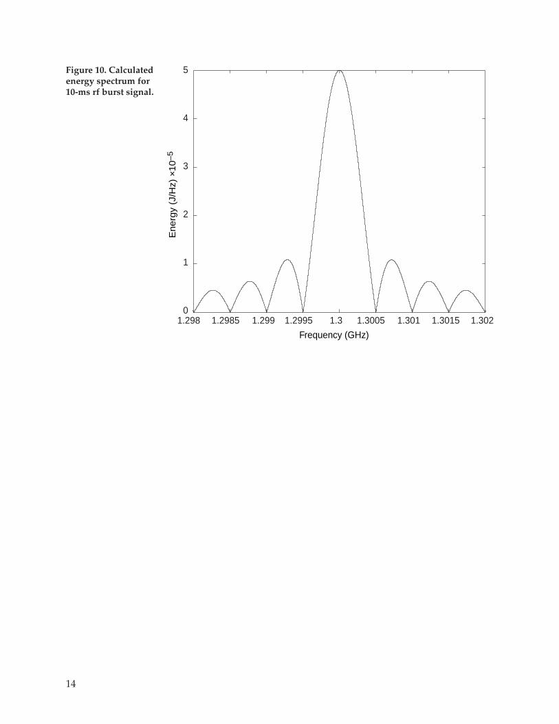
The FFT results for q0(t)/2 and pz(t) are shown in figures 8(a) and 8(b),respectively. The spectral envelope depends primarily on T with finefeatures related to T1, while the number of impulses depends on T2.Truncation of the transient to an rf burst signal does not affect the FFTresult or the power spectrum as measured on a spectrum analyzer. How-ever, the total average energy transmitted is proportional to the duration(or dwell time) so that the average energy is obtained by scaling thepower spectrum by tmax. The frequency-shifted energy spectrum for a 50-pulse burst is shown in figure 9, where the amplitude is based on a peaktransmitted power of 30 dBm (1 W). When only the spectral envelopeB0(ω) is of interest, it can be calculated directly (with the appropriatenormalization). The calculated energy is shown in figure 10 and repre-sents the average energy spectral envelope. The energy spectrum is still asequence of impulses at the modulation repetition frequencies as shownin figure 9, with magnitude defined by this envelope.
1Papoulis, A., The Fourier Integral and Its Applications, New York, NY: McGraw-Hill (1987).
12
Figure 7. (a) Modulation waveform for 50-pulse rf burst, (b) scaled FFT result shifted to modulatedcarrier, (c) FFT result (times one-half) over 80-kHz span for comparison to figure 4(c), and (d) FFTresult (times one-half) over 20-kHz span to show spectral line characteristics.
Time (s)
Am
plitu
de
1
0.9
0.8
0.7
0.6
0.5
0.4
0.3
0.2
0.1
0 0 0.001 0.002 0.003 0.004 0.005 0.006 0.007 0.008 0.009 0.01
Frequency (GHz)
Mag
nitu
de (
1/H
z) ×
10–3
5
4.5
4
3.5
3
2.5
2
1.5
1
0.5
01.298 1.2985 1.299 1.2995 1.3 1.3005 1.301 1.3015
Mag
nitu
de (
1/H
z) ×
10–3
Frequency (Hz) ×104
5
4.5
4
3.5
3
2.5
2
1.5
1
0.5
0–4 –3 –2 –1 0 1 2 3 4
Mag
nitu
de (
1/H
z) ×
10–3
Frequency (Hz) ×104–1 –0.8 –0.6 –0.4 –0.2 0 0.2 0.4 0.6 0.8 1
5
4.5
4
3.5
3
2.5
2
1.5
1
0.5
0
(a) (b)
(c) (d)

13
Figure 9. Energyspectrum byconvolution of FFTresults.
Frequency (GHz)
En
erg
y (J
/Hz)
×1
0–
5
1.298 1.2985 1.299 1.2995 1.3 1.3005 1.301 1.3015 1.302
5
4
3
2
1
0
Figure 8. (a) FFT result(times one-half) fortwo periods ofmodulation waveformand (b) FFT result fortruncation timewindow.
Mag
nitu
de (
1/H
z) ×
10–3 5
4
3
2
1
0–2 –1.5 –1 –0.5 0 0.5 1 1.5 2
Frequency (MHz)
(a)
(b)
Frequency (MHz)
Mag
nitu
de (
1/H
z) ×
10–3 1
0.8
0.6
0.4
0.2
0–1000 –800 –600 –400 –200 0 200 400 600 800 1000
14
Figure 10. Calculatedenergy spectrum for10-ms rf burst signal.
Frequency (GHz)
En
erg
y (J
/Hz)
×1
0–5
5
4
3
2
1
01.298 1.2985 1.299 1.2995 1.3 1.3005 1.301 1.3015 1.302
15
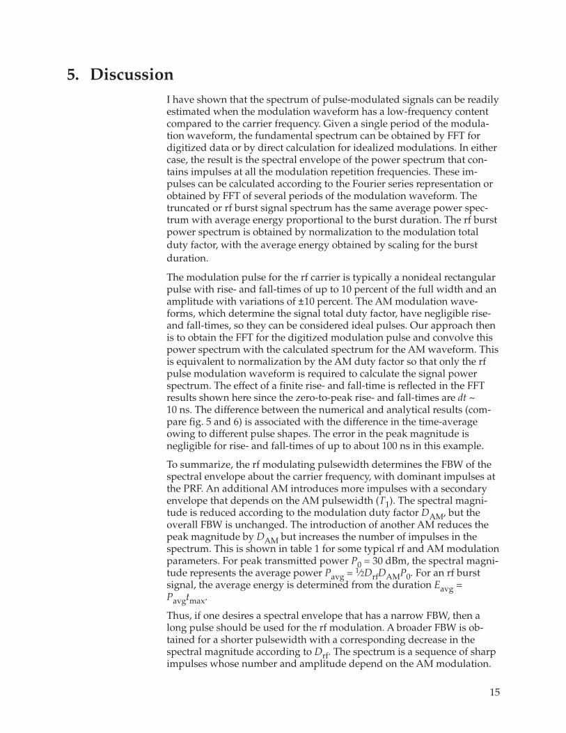
5. DiscussionI have shown that the spectrum of pulse-modulated signals can be readilyestimated when the modulation waveform has a low-frequency contentcompared to the carrier frequency. Given a single period of the modula-tion waveform, the fundamental spectrum can be obtained by FFT fordigitized data or by direct calculation for idealized modulations. In eithercase, the result is the spectral envelope of the power spectrum that con-tains impulses at all the modulation repetition frequencies. These im-pulses can be calculated according to the Fourier series representation orobtained by FFT of several periods of the modulation waveform. Thetruncated or rf burst signal spectrum has the same average power spec-trum with average energy proportional to the burst duration. The rf burstpower spectrum is obtained by normalization to the modulation totalduty factor, with the average energy obtained by scaling for the burstduration.
The modulation pulse for the rf carrier is typically a nonideal rectangularpulse with rise- and fall-times of up to 10 percent of the full width and anamplitude with variations of ±10 percent. The AM modulation wave-forms, which determine the signal total duty factor, have negligible rise-and fall-times, so they can be considered ideal pulses. Our approach thenis to obtain the FFT for the digitized modulation pulse and convolve thispower spectrum with the calculated spectrum for the AM waveform. Thisis equivalent to normalization by the AM duty factor so that only the rfpulse modulation waveform is required to calculate the signal powerspectrum. The effect of a finite rise- and fall-time is reflected in the FFTresults shown here since the zero-to-peak rise- and fall-times are dt ~10␣ ns. The difference between the numerical and analytical results (com-pare fig. 5 and 6) is associated with the difference in the time-averageowing to different pulse shapes. The error in the peak magnitude isnegligible for rise- and fall-times of up to about 100 ns in this example.
To summarize, the rf modulating pulsewidth determines the FBW of thespectral envelope about the carrier frequency, with dominant impulses atthe PRF. An additional AM introduces more impulses with a secondaryenvelope that depends on the AM pulsewidth (T1). The spectral magni-tude is reduced according to the modulation duty factor DAM, but theoverall FBW is unchanged. The introduction of another AM reduces thepeak magnitude by DAM but increases the number of impulses in thespectrum. This is shown in table 1 for some typical rf and AM modulationparameters. For peak transmitted power P0 = 30 dBm, the spectral magni-tude represents the average power Pavg = 1⁄2DrfDAMP0. For an rf burstsignal, the average energy is determined from the duration Eavg =Pavgtmax.
Thus, if one desires a spectral envelope that has a narrow FBW, then along pulse should be used for the rf modulation. A broader FBW is ob-tained for a shorter pulsewidth with a corresponding decrease in thespectral magnitude according to Drf. The spectrum is a sequence of sharpimpulses whose number and amplitude depend on the AM modulation.
16
However, the overall power spectrum envelope is determined by the rfmodulation with peak magnitude given by the time-average of the rfsignal. Given a fixed Drf, the total average power with AM is reduced byDAM unless P0 is increased to maintain the same time-average. Alterna-tively, for fixed transmitted power, Drf must be increased to compensatefor DAM to obtain the same average power in the transmitted signal. Interms of average energy, the duration is a parameter, so different combi-nations of rf and AM modulations could have equivalent Eavg in thetransmitted signal as shown in table 1. The rf pulsewidth and the lowestmodulation repetition frequency are the important parameters for thespectral content of the transmitted signal, while the modulation dutyfactors control the spectral amplitude. The rf and AM parameters can beappropriately adjusted to obtain a desired power spectrum with theenergy spectrum determined by the duration of the rf burst signal.
rf modulation AMparameters (µs) parameters (ms) Impulse
FWB frequency Pavg EavgT T0 tmax T1 T2 (kHz) (kHz) (mW) (nJ)
2 1000 500 — — 1000 1 1 5002 200 100 — — 1000 5 5 5002 50 25 — — 1000 20 20 5002 50 100 0.25 1 1000 1 5 5002 50 100 0.5 2 1000 0.5 5 500
10 2000 200 — — 200 0.5 2.5 50010 2000 400 2 4 200 0.25 1.25 50010 1000 200 2 4 200 0.25 2.5 50010 200 80 0.5 2 200 0.5 6.25 50030 2000 67 — — 67 0.5 7.5 50030 2000 133 2 4 67 0.25 3.75 500— — 200 0.05 10 40 0.1 2.5 500
Table 1. Spectralcharacteristics of an rfburst of duration tmaxand 1-W peaktransmitted power.
17
Distribution
AdmnstrDefns Techl Info CtrAttn DTIC-OCP8725 John J Kingman Rd Ste 0944FT Belvoir VA 22060-6218
Ofc of the Secy of DefnsAttn ODDRE (R&AT)The PentagonWashington DC 20301-3080
OSDAttn OUSD(A&T)/ODDR&E(R) R J TrewWashington DC 20301-7100
AMCOM MRDECAttn AMSMI-RD W C McCorkleRedstone Arsenal AL 35898-5240
Dir for MANPRINTOfc of the Deputy Chief of Staff for PrsnnlAttn J HillerThe Pentagon Rm 2C733Washington DC 20301-0300
Pacific Northwest National LaboatoryAttn K8-41 R ShippellPO Box 999Richland WA 99352
US Army ARDECAttn AMSTA-CCL H Moore Bldg 65NPicatinny Arsenal NJ 07806-5000
US Army Armament Rsrch Dev & Engrg CtrAttn AMSTA-AR-TD M FisetteBldg 1Picatinny Arsenal NJ 07806-5000
US Army Edgewood RDECAttn SCBRD-TD G ResnickAberdeen Proving Ground MD 21010-5423
US Army Info Sys Engrg CmndAttn ASQB-OTD F JeniaFT Huachuca AZ 85613-5300
US Army Natick RDEC Acting Techl DirAttn SSCNC-T P BrandlerNatick MA 01760-5002
DirectorUS Army Rsrch Ofc4300 S Miami BlvdResearch Triangle Park NC 27709
US Army Simulation, Train, & InstrmntnCmnd
Attn J Stahl12350 Research ParkwayOrlando FL 32826-3726
US Army Tank-Automtv Cmnd Rsrch, Dev, &Engrg Ctr
Attn AMSTA-TA J ChapinWarren MI 48397-5000
US Army Train & Doctrine Cmnd Battle LabIntegration & Techl Dirctrt
Attn ATCD-B J A KleveczFT Monroe VA 23651-5850
Nav Surface Warfare CtrAttn Code B07 J Pennella17320 Dahlgren Rd Bldg 1470 Rm 1101Dahlgren VA 22448-5100
DARPAAttn B Kaspar3701 N Fairfax DrArlington VA 22203-1714
Hicks & Associates IncAttn G Singley III1710 Goodrich Dr Ste 1300McLean VA 22102
US Army Rsrch LabAttn AMSRL-CI-LL Techl Lib (3 copies)Attn AMSRL-CS-AS Mail & Records MgmtAttn AMSRL-CS-EA-TP Techl Pub (3 copies)Attn AMSRL-SE-DE C ReiffAttn AMSRL-SE-DE J MilettaAttn AMSRL-SE-DS J TuttleAttn AMSRL-SE-DS L JasperAttn AMSRL-SE-DS W O Coburn (10 copies)Adelphi MD 20783-1197
1. AGENCY USE ONLY
8. PERFORMING ORGANIZATION REPORT NUMBER
7. PERFORMING ORGANIZATION NAME(S) AND ADDRESS(ES)
12a. DISTRIBUTION/AVAILABILITY STATEMENT
10. SPONSORING/MONITORING AGENCY REPORT NUMBER
5. FUNDING NUMBERS4. TITLE AND SUBTITLE
6. AUTHOR(S)
REPORT DOCUMENTATION PAGE
3. REPORT TYPE AND DATES COVERED2. REPORT DATE
11. SUPPLEMENTARY NOTES
14. SUBJECT TERMS
13. ABSTRACT (Maximum 200 words)
Form ApprovedOMB No. 0704-0188
(Leave blank)
9. SPONSORING/MONITORING AGENCY NAME(S) AND ADDRESS(ES)
Public reporting burden for this collection of information is estimated to average 1 hour per response, including the time for reviewing instructions, searching existing data sources,gathering and maintaining the data needed, and completing and reviewing the collection of information. Send comments regarding this burden estimate or any other aspect of thiscollection of information, including suggestions for reducing this burden, to Washington Headquarters Services, Directorate for Information Operations and Reports, 1215 JeffersonDavis Highway, Suite 1204, Arlington, VA 22202-4302, and to the Office of Management and Budget, Paperwork Reduction Project (0704-0188), Washington, DC 20503.
12b. DISTRIBUTION CODE
15. NUMBER OF PAGES
16. PRICE CODE
17. SECURITY CLASSIFICATION OF REPORT
18. SECURITY CLASSIFICATION OF THIS PAGE
19. SECURITY CLASSIFICATION OF ABSTRACT
20. LIMITATION OF ABSTRACT
NSN 7540-01-280-5500 Standard Form 298 (Rev. 2-89)Prescribed by ANSI Std. Z39-18298-102
Spectral Analysis of Pulse-Modulated rf Signals
September 1999 Final, January to June 1999
The parameters that characterize a rectangular-shaped pulse-modulated sinusoidal signal are thecarrier frequency, the pulsewidth, the repetition frequency, and the number of pulses in or theduration of the signal. We use a Fourier series representation to show the influence of theseparameters on the spectrum of a pulse-modulated signal at a microwave carrier frequency. Whenan additional amplitude modulation is applied at audio frequencies, the resulting transient cannotbe efficiently analyzed with numerical transform techniques. We present approximate numericaland analytical techniques to obtain the frequency spectrum of such signals. This approach allowsthe near-real-time spectral analysis of modulated signals. Thus, the resulting spectrum can beeasily calculated for idealized modulation waveforms. A typical example is presented and theeffect of pulse modulation on the spectral content of an rf signal burst is discussed.
Pulse modulation, amplitude, power spectrum
Unclassified
ARL-TN-152
9NEYYY622120.140
A14062120A
ARL PR:AMS code:
DA PR:PE:
Approved for public release;distribution unlimited.
24
Unclassified Unclassified UL
2800 Powder Mill RoadAdelphi, MD 20783-1197
U.S. Army Research LaboratoryAttn: AMSRL- SE-DS [email protected]
U.S. Army Research Laboratory
19
William O. Coburn
email:2800 Powder Mill RoadAdelphi, MD 20783-1197

DE
PA
RT
ME
NT
OF
TH
E A
RM
YU
.S.
Arm
y R
esea
rch
Lab
orat
ory
2800
Pow
der
Mill
Roa
dA
del
phi
, MD
20
783-
1197
An
Equ
al O
pp
ortu
nity
Em
plo
yer