Spectral Properties of

Spectral Properties ofBanded Toeplitz Matrices

ot99Bottcher FM1.qxp 10/6/2005 10:27 AM Page 1


Spectral Properties ofBanded Toeplitz Matrices

Albrecht BöttcherChemnitz University of TechnologyChemnitz, Germany

Sergei M. GrudskyCINVESTAV del I. P. N. Mexico City, MexicoandRostov-on-Don State UniversityRostov-on-Don, Russia

Society for Industrial and Applied MathematicsPhiladelphia


Copyright © 2005 by the Society for Industrial and Applied Mathematics.

10 9 8 7 6 5 4 3 2 1

All rights reserved. Printed in the United States of America. No part of this book may be reproduced,stored, or transmitted in any manner without the written permission of the publisher. For information,write to the Society for Industrial and Applied Mathematics, 3600 University City Science Center,Philadelphia, PA 19104-2688.

MATLAB® is a registered trademark of The MathWorks, Inc. and is used with permission. TheMathWorks does not warrant the accuracy of the text or exercises in this book. This book’s use or discussion of MATLAB® software or related products does not constitute endorsement or sponsorship by The MathWorks of a particular pedagogical approach or particular use of the MATLAB® software. For MATLAB® product information, please contact The MathWorks, Inc., 3 Apple Hill Drive, Natick, MA 01760-2098 USA, 508-647-7000, Fax: 508-647-7101,[email protected], www.mathworks.com/

Library of Congress Cataloging-in-Publication Data

Böttcher, Albrecht.Spectral properties of banded Toeplitz matrices / Albrecht Böttcher, Sergei M. Grudsky.

p. cm.Includes bibliographical references and index.ISBN 0-89871-599-7 (pbk.)

Toeplitz matrices. I. Grudsky, Sergei M., 1955- II. Title.

QA188.B674 2005512.9’434—dc22

2005051608

is a registered trademark.

Partial royalties from the sale of this book are placed in a fund to help students attendSIAM meetings and other SIAM-related activities. This fund is administered by SIAM,and qualified individuals are encouraged to write directly to SIAM for guidelines.


buch72005/10/5page v

�

�

�

�

�

�

�

�

Contents

Preface ix

1 Infinite Matrices 11.1 Toeplitz and Hankel Matrices . . . . . . . . . . . . . . . . . . . . . . 11.2 Boundedness . . . . . . . . . . . . . . . . . . . . . . . . . . . . . . . 21.3 Products . . . . . . . . . . . . . . . . . . . . . . . . . . . . . . . . . 51.4 Wiener-Hopf Factorization . . . . . . . . . . . . . . . . . . . . . . . 61.5 Spectra . . . . . . . . . . . . . . . . . . . . . . . . . . . . . . . . . . 91.6 Norms . . . . . . . . . . . . . . . . . . . . . . . . . . . . . . . . . . 101.7 Inverses . . . . . . . . . . . . . . . . . . . . . . . . . . . . . . . . . 121.8 Eigenvalues and Eigenvectors . . . . . . . . . . . . . . . . . . . . . . 151.9 Selfadjoint Operators . . . . . . . . . . . . . . . . . . . . . . . . . . 21

2 Determinants 312.1 Circulant Matrices . . . . . . . . . . . . . . . . . . . . . . . . . . . . 312.2 Tridiagonal Toeplitz Matrices . . . . . . . . . . . . . . . . . . . . . . 342.3 The Baxter-Schmidt Formula . . . . . . . . . . . . . . . . . . . . . . 362.4 Widom’s Formula . . . . . . . . . . . . . . . . . . . . . . . . . . . . 382.5 Trench’s Formula . . . . . . . . . . . . . . . . . . . . . . . . . . . . 412.6 Szegö’s Strong Limit Theorem . . . . . . . . . . . . . . . . . . . . . 432.7 The Szegö-Widom Theorem . . . . . . . . . . . . . . . . . . . . . . . 452.8 Geronimo, Case, Borodin, Okounkov . . . . . . . . . . . . . . . . . . 48

3 Stability 593.1 Strong and Weak Convergence . . . . . . . . . . . . . . . . . . . . . 593.2 Stable Sequences . . . . . . . . . . . . . . . . . . . . . . . . . . . . 613.3 The Baxter-Gohberg-Feldman Theorem . . . . . . . . . . . . . . . . . 623.4 Silbermann Theory . . . . . . . . . . . . . . . . . . . . . . . . . . . 643.5 Asymptotic Inverses . . . . . . . . . . . . . . . . . . . . . . . . . . . 68

4 Instability 794.1 Outside the Essential Spectrum . . . . . . . . . . . . . . . . . . . . . 794.2 Exponential Growth Is Generic . . . . . . . . . . . . . . . . . . . . . 804.3 Arbitrarily Fast Growth . . . . . . . . . . . . . . . . . . . . . . . . . 83

v

buch72005/10/5page vi

�

�

�

�

�

�

�

�

vi Contents

4.4 Sequences Versus Polynomials . . . . . . . . . . . . . . . . . . . . . 854.5 Symbols with Zeros: Lower Estimates . . . . . . . . . . . . . . . . . 884.6 Symbols with Zeros: Upper Estimates . . . . . . . . . . . . . . . . . 904.7 Inside the Essential Spectrum . . . . . . . . . . . . . . . . . . . . . . 964.8 Semi-Definite Matrices . . . . . . . . . . . . . . . . . . . . . . . . . 101

5 Norms 1135.1 A Universal Estimate . . . . . . . . . . . . . . . . . . . . . . . . . . 1135.2 Spectral Norm of Toeplitz Matrices . . . . . . . . . . . . . . . . . . . 1175.3 Fejér Means . . . . . . . . . . . . . . . . . . . . . . . . . . . . . . . 1215.4 Toeplitz-Like Matrices . . . . . . . . . . . . . . . . . . . . . . . . . . 1235.5 Exponentially Fast Convergence Is Generic . . . . . . . . . . . . . . . 1265.6 Slow Convergence . . . . . . . . . . . . . . . . . . . . . . . . . . . . 1315.7 Summary . . . . . . . . . . . . . . . . . . . . . . . . . . . . . . . . . 132

6 Condition Numbers 1376.1 Asymptotic Inverses of Toeplitz-Like Matrices . . . . . . . . . . . . . 1376.2 The Limit of the Condition Numbers . . . . . . . . . . . . . . . . . . 1396.3 Convergence Speed Estimates . . . . . . . . . . . . . . . . . . . . . . 1426.4 Generic and Exceptional Cases . . . . . . . . . . . . . . . . . . . . . 1456.5 Norms of Inverses of Pure Toeplitz Matrices . . . . . . . . . . . . . . 1476.6 Condition Numbers of Pure Toeplitz Matrices . . . . . . . . . . . . . 1536.7 Conclusions . . . . . . . . . . . . . . . . . . . . . . . . . . . . . . . 154

7 Substitutes for the Spectrum 1577.1 Pseudospectra . . . . . . . . . . . . . . . . . . . . . . . . . . . . . . 1577.2 Norm of the Resolvent . . . . . . . . . . . . . . . . . . . . . . . . . . 1597.3 Limits of Pseudospectra . . . . . . . . . . . . . . . . . . . . . . . . . 1637.4 Pseudospectra of Infinite Toeplitz Matrices . . . . . . . . . . . . . . . 1657.5 Numerical Range . . . . . . . . . . . . . . . . . . . . . . . . . . . . 1657.6 Collective Perturbations . . . . . . . . . . . . . . . . . . . . . . . . . 170

8 Transient Behavior 1778.1 The General Message . . . . . . . . . . . . . . . . . . . . . . . . . . 1778.2 Polynomial Numerical Hulls . . . . . . . . . . . . . . . . . . . . . . 1798.3 The Pseudospectra Perspective . . . . . . . . . . . . . . . . . . . . . 1818.4 A Triangular Example . . . . . . . . . . . . . . . . . . . . . . . . . . 1868.5 Gauss-Seidel for Large Toeplitz Matrices . . . . . . . . . . . . . . . . 1878.6 Genuinely Finite Results . . . . . . . . . . . . . . . . . . . . . . . . . 1928.7 The Sky Region Contains an Angle . . . . . . . . . . . . . . . . . . . 1958.8 Oscillations . . . . . . . . . . . . . . . . . . . . . . . . . . . . . . . 2008.9 Exponentials . . . . . . . . . . . . . . . . . . . . . . . . . . . . . . . 204

9 Singular Values 2119.1 Approximation Numbers . . . . . . . . . . . . . . . . . . . . . . . . 2119.2 The Splitting Phenomenon . . . . . . . . . . . . . . . . . . . . . . . 212

buch72005/10/5page vii

�

�

�

�

�

�

�

�

Contents vii

9.3 Singular Values of Circulant Matrices . . . . . . . . . . . . . . . . . . 2159.4 Extreme Singular Values . . . . . . . . . . . . . . . . . . . . . . . . . 2169.5 The Limiting Set . . . . . . . . . . . . . . . . . . . . . . . . . . . . . 2179.6 The Limiting Measure . . . . . . . . . . . . . . . . . . . . . . . . . . 2199.7 Proper Clusters . . . . . . . . . . . . . . . . . . . . . . . . . . . . . . 2249.8 Norm of Matrix Times Random Vector . . . . . . . . . . . . . . . . . 2259.9 The Case of Toeplitz and Circulant Matrices . . . . . . . . . . . . . . 2299.10 The Nearest Structured Matrix . . . . . . . . . . . . . . . . . . . . . 233

10 Extreme Eigenvalues 24510.1 Hermitian Matrices . . . . . . . . . . . . . . . . . . . . . . . . . . . 24510.2 First-Order Trace Formulas . . . . . . . . . . . . . . . . . . . . . . . 24810.3 The Spectral Radius . . . . . . . . . . . . . . . . . . . . . . . . . . . 25010.4 Matrices with Nonnegative Entries . . . . . . . . . . . . . . . . . . . 253

11 Eigenvalue Distribution 26111.1 Toward the Limiting Set . . . . . . . . . . . . . . . . . . . . . . . . . 26111.2 Structure of the Limiting Set . . . . . . . . . . . . . . . . . . . . . . 26411.3 Toward the Limiting Measure . . . . . . . . . . . . . . . . . . . . . . 26711.4 Limiting Set and Limiting Measure . . . . . . . . . . . . . . . . . . . 27111.5 Connectedness of the Limiting Set . . . . . . . . . . . . . . . . . . . 275

12 Eigenvectors and Pseudomodes 28712.1 Tridiagonal Circulant and Toeplitz Matrices . . . . . . . . . . . . . . 28712.2 Eigenvectors of Triangular and Tridiagonal Matrices . . . . . . . . . . 28812.3 Asymptotics of Eigenvectors . . . . . . . . . . . . . . . . . . . . . . 29412.4 Pseudomodes of Circulant Matrices . . . . . . . . . . . . . . . . . . . 30012.5 Pseudomodes of Toeplitz Matrices . . . . . . . . . . . . . . . . . . . 303

13 Structured Perturbations 30913.1 Toeplitz Pseudospectra . . . . . . . . . . . . . . . . . . . . . . . . . 30913.2 The Nearest Singular Matrix . . . . . . . . . . . . . . . . . . . . . . 31013.3 Structured Normwise Condition Numbers . . . . . . . . . . . . . . . 31313.4 Toeplitz Systems . . . . . . . . . . . . . . . . . . . . . . . . . . . . . 31713.5 Exact Right-Hand Sides . . . . . . . . . . . . . . . . . . . . . . . . . 32013.6 The Condition Number for Matrix Inversion . . . . . . . . . . . . . . 32813.7 Once More the Nearest Singular Matrix . . . . . . . . . . . . . . . . . 330

14 Impurities 33514.1 The Discrete Laplacian . . . . . . . . . . . . . . . . . . . . . . . . . 33514.2 An Uncertain Block . . . . . . . . . . . . . . . . . . . . . . . . . . . 34114.3 Emergence of Antennae . . . . . . . . . . . . . . . . . . . . . . . . . 34714.4 Behind the Black Hole . . . . . . . . . . . . . . . . . . . . . . . . . . 35314.5 Can Structured Pseudospectra Jump? . . . . . . . . . . . . . . . . . . 362

Bibliography 387

Index 407

buch72005/10/5page viii

�

�

�

�

�

�

�

�

buch72005/10/5page ix

�

�

�

�

�

�

�

�

Preface

Toeplitz matrices emerge in plenty of applications and have been extensively studied forabout a century. The literature on them is immense and ranges from thousands of articles inperiodicals to huge monographs. This does not imply that there is nothing left to say on thetopic. To the contrary, Toeplitz matrices are an active field of research with many facets, andthe amount of material gathered only in the last decade would easily fill several volumes.

The present book lives within its limitations: to banded Toeplitz matrices on the onehand and to the spectral properties of such matrices on the other. As a third limitation, weconsider large matrices only, and most of the results are actually asymptotics.

When speaking of banded Toeplitz matrices, we have in mind an n × n Toeplitzmatrix of bandwidth 2r + 1, and we silently assume that n is large in comparison with2r + 1. A Toeplitz matrix is completely specified by the (complex) numbers that constituteits first row and its first column. The function on the complex unit circle whose Fouriercoefficients are just these numbers is referred to as the symbol of the matrix. In the caseof Toeplitz band matrices, the symbol is a Laurent polynomial. Thus, we need not strugglewith piecewise continuous or oscillating symbols, which arise in many applications, but“only” with Laurent polynomials. This circumstance simplifies part of the investigation.On the other hand, Laurent polynomials cause questions that are different from those oneencounters in connection with more general symbols. Eventually, Toeplitz band matricesform their own realm in the world of Toeplitz matrices.

We understand spectral properties in a broad sense. Of course, we study such problemsas the evolution of the eigenvalues of banded n×nToeplitz matrices as n goes to infinity. Thepioneering result in this direction was already proved by Schmidt and Spitzer in 1960, andevery worker in the field has a personal copy of the Schmidt/Spitzer paper. Here we cite a fullproof of this result for the first time in the monographical literature. This proof is Schmidtand Spitzer’s original proof with several simplifications and improvements introduced byHirschman and Widom.

We regard the singular values of a matrix as its most important spectral characteristicsafter the eigenvalues and pseudoeigenvalues; hence, we pay due attention to the asymptoticbehavior of the singular values as the matrix dimension increases to infinity. Clearly, ques-tions about the norm, the norm of the inverse, and the condition numbers of a matrix arequestions about the extreme singular values.

Normal Toeplitz matrices raise specific problems, and these will be discussed. How-ever, typically a Toeplitz matrix is nonnormal; hence, pseudospectra tell us more aboutToeplitz matrices than spectra. Accordingly, we embark on pseudospectra of Toeplitz matri-ces and on related issues, such as the transient behavior of powers of large Toeplitz matrices.

ix

buch72005/10/5page x

�

�

�

�

�

�

�

�

x Preface

Finally, the book contains some very recent results on the spectral behavior of Toeplitzmatrices under certain structured perturbations. These results are far from what one wants toknow about Toeplitz matrices with randomly perturbed main diagonal, but they are beautiful,they point in a good direction, and they have the potential to stimulate further research.

As already stated, the majority of the results describe the asymptotic behavior as thematrix dimension n goes to infinity. Many questions considered here can be easily answeredby a few MATLAB commands if the matrix dimension is moderate, say in the low hundreds.We try to deliver answers in the case where n is really large and the computer quits. Part ofthe results are equipped with estimates of the convergence speed, which provides the user atleast with a vague feeling for as to whether one can invoke the result for n in the hundreds.And, most importantly, several problems of this book are motivated by applications instatistical physics, where n is around 108, the cube root of the Avogadro number 1023, and,for such astronomic values of n, asymptotic formulas are the only chance to describe andto understand something.

In summary, the book provides several pieces of information about the eigenval-ues, singular values, determinants, norms, norms of inverses, (unstructured and structured)condition numbers, (unstructured and structured) pseudospectra, transient behavior, eigen-vectors and pseudomodes, and spectral phenomena caused by perturbations of large Toeplitzband matrices. The selection of the material represents our taste and is to some extent de-termined by subjects we have worked on ourselves, and we think we can tell the communitysomething about. Naturally, numerous problems are left open. Moreover, various importanttopics, such as fast inversion of Toeplitz matrices or fast solution of Toeplitz systems, arenot touched at all. These topics are the business of other books (see, for example, [157]and [177]). However, the material of the present book is certainly useful and in many caseseven indispensable when dealing with such practical problems as the effective solution of alarge banded Toeplitz system.

The book is intended as an introductory text to some advanced topics. We assumethat the reader is familiar with the basics of real and complex analysis, linear algebra, andfunctional analysis. Almost all results are accompanied by full proofs.

A baby version of this book was published under the title Toeplitz Matrices, AsymptoticLinear Algebra, and Functional Analysis by Hindustan Book Agency, New Delhi, andBirkhäuser, Basel, in 2000.

S. M. Grudsky thankfully acknowledges financial support by CONACYT grantN 40564-F (México).

We sincerely thank our wives, Sylvia Böttcher and Olga Grudskaya, for their usualpatient and excellent work on the LATEX masters and on part of the illustrations. We are alsogreatly indebted to Mark Embree for valuable remarks on a draft of this book and to LindaThiel and the staff of SIAM for their help with publishing the book.

Tragically, Olga Grudskaya died in a car accident in February 2004. We have lost anexceptional woman, a wonderful friend, and an irreplaceable colleague. Her early deathleaves an emptiness that can never be filled. In late 2003, she began working on the illustra-tions for this book with great enthusiasm. She could not accomplish her visions. We wereleft with the drafts of her illustrations and included some of them. They provide us with anidea of the beauty that would have emerged if she would have been able to complete herwork. May this book keep the memory of our irretrievable Olga.

Chemnitz and Mexico City, spring 2005 The authors

buch72005/10/5page 1

�

�

�

�

�

�

�

�

Chapter 1

Infinite Matrices

When studying large finite matrices, it is natural to look also at their infinite counterparts.The spectral phenomena of the latter are sometimes easier to understand than those of theformer. The question whether properties of infinite Toeplitz matrices mimic the correspond-ing properties of their large finite sections is very delicate and is, in a sense, the topic of thisbook.

We regard infinite Toeplitz matrices as operators on �p. This chapter is concernedwith some basic properties of these operators, including boundedness, norms, invertibilityand inverses, spectrum, eigenvalues, and eigenvectors. Wiener-Hopf factorization providesus with a fairly effective tool for the inversion of infinite (but not of finite) Toeplitz matrices.We also embark on some of the problems that are specific for selfadjoint operators.

1.1 Toeplitz and Hankel MatricesAn infinite Toeplitz matrix is a matrix of the form

(aj−k)∞j,k=0 =

⎛⎜⎜⎝a0 a−1 a−2 . . .

a1 a0 a−1 . . .

a2 a1 a0 . . .

. . . . . . . . . . . .

⎞⎟⎟⎠ . (1.1)

Such matrices are characterized by the property of being constant along the parallels to themain diagonal. Clearly, the matrix (1.1) is completely determined by its entries in the firstrow and first column, that is, by the sequence

{ak}∞k=−∞ = { . . . , a−2, a−1, a0, a1, a2, . . . }. (1.2)

Throughout this book we assume that the ak’s are complex numbers.The matrix (1.1) is a band matrix if and only if at most finitely many of the numbers

in (1.2) are nonzero. Although our subject is Toeplitz band matrices, it is also necessary tostudy Toeplitz matrices which are not band matrices. For example, the inverse of the band

1


�

�

�

�

�

�

�

�

2 Chapter 1. Infinite Matrices

matrix ⎛⎜⎜⎜⎜⎜⎝1 − 1

2 0 0 . . .

0 1 − 12 0 . . .

0 0 1 − 12 . . .

0 0 0 1 . . .

. . . . . . . . . . . . . . .

⎞⎟⎟⎟⎟⎟⎠is the Toeplitz matrix ⎛⎜⎜⎜⎜⎜⎝

1 12

122

123 . . .

0 1 12

122 . . .

0 0 1 12 . . .

0 0 0 1 . . .

. . . . . . . . . . . . . . .

⎞⎟⎟⎟⎟⎟⎠ ,

and this is not a band matrix.There is another type of matrix that arises when working with Toeplitz matrices. These

are the Hankel matrices. An infinite Hankel matrix has the form

(aj+k+1)∞j,k=0 =

⎛⎜⎜⎝a1 a2 a3 . . .

a2 a3 . . . . . .

a3 . . . . . . . . .

. . . . . . . . . . . .

⎞⎟⎟⎠ . (1.3)

Notice that (1.3) is completely given by only the numbers with positive indices in (1.2).Obviously, if the sequence (1.2) has finite support, then the matrix (1.3) contains onlyfinitely many nonzero entries.

1.2 BoundednessThe Wiener algebra. Let T := {t ∈ C : |t | = 1} be the complex unit circle. The Wieneralgebra W is defined as the set of all functions a : T → C with absolutely convergent Fourierseries - that is, as the collection of all functions a : T → C which can be represented in theform

a(t) =∞∑

n=−∞ant

n (t ∈ T) with ‖a‖W :=∞∑

n=−∞|an| <∞. (1.4)

Notice that instead of (1.4) we could also write

a(eiθ ) =∞∑

n=−∞ane

inθ (eiθ ∈ T) with ‖a‖W :=∞∑

n=−∞|an| <∞. (1.5)

The numbers an are the Fourier coefficients of a, and they can be computed by the formula

an = 1

2π

∫ 2π

0a(eiθ )e−inθ dθ. (1.6)


�

�

�

�

�

�

�

�

1.2. Boundedness 3

Sometimes it will be convenient to identify a function a : T → C with the functionθ �→ a(eiθ ); the latter function may be thought of as being given on [0, 2π), (−π, π ],or even on all of the real line R. Clearly, functions in W are continuous on T and, whenregarded as functions on R, they are 2π -periodic continuous functions.

Now let a ∈ W and let {an}∞n=−∞ be the sequence of the Fourier coefficients of a. Wedenote by T (a) and H(a) the matrices (1.1) and (1.3), respectively:

T (a) :=

⎛⎜⎜⎝a0 a−1 a−2 . . .

a1 a0 a−1 . . .

a2 a1 a0 . . .

. . . . . . . . . . . .

⎞⎟⎟⎠ , H(a) :=

⎛⎜⎜⎝a1 a2 a3 . . .

a2 a3 . . . . . .

a3 . . . . . . . . .

. . . . . . . . . . . .

⎞⎟⎟⎠ .

The matrix T (a) is called the infinite Toeplitz matrix generated by a, while a is referredto as the symbol of the matrix T (a). Note that if

∑∞n=−∞ |an| < ∞, then there is exactly

one a ∈ W such that (1.6) holds for all n. On the other hand, although H(a) is uniquelydetermined by a, it is only the numbers an with n ≥ 1 that can be recovered from the matrixH(a). In other words: H(a) = H(b) if and only if an = bn for all n ≥ 1.

Infinite matrices as operators. We let �p := �p(Z+) (1 ≤ p ≤ ∞) stand for the usualBanach spaces of complex-valued sequences {xn}∞n=0: for 1 ≤ p <∞,

x = {xn}∞n=0 ∈ �p ⇐⇒ ‖x‖pp :=

∞∑n=0

|xn|p <∞,

and for p = ∞,

x = {xn}∞n=0 ∈ �∞ ⇐⇒ ‖x‖∞ := supn≥0|xn| <∞.

An infinite matrix A = (ajk)∞j,k=0 is said to induce a bounded operator on �p if there is a

constant M ∈ (0,∞) such that for every x = {xn}∞n=0 ∈ �p the inequality

∞∑j=0

∣∣∣ ∞∑k=0

ajkxk

∣∣∣p ≤ Mp

∞∑k=0

|xk|p (1.7)

holds; we remark that (1.7) includes the requirement that the series

yj =∞∑

k=0

ajkxk (j ≥ 0) and∞∑

j=0

|yj |p

are convergent. If A = (ajk)∞j,k=0 induces a bounded operator on �p, we can simply think

of A as being a bounded operator on �p which, after writing the elements of �p as columnvectors, acts by the rule

y = Ax with

⎛⎜⎜⎜⎝y0

y1

y2...

⎞⎟⎟⎟⎠ =

⎛⎜⎜⎜⎝a00 a01 a02 . . .

a10 a11 a12 . . .

a20 a21 a22 . . ....

......

⎞⎟⎟⎟⎠⎛⎜⎜⎜⎝

x0

x1

x2...

⎞⎟⎟⎟⎠ .


�

�

�

�

�

�

�

�


If A induces a bounded operator on �p, then there is a smallest M for which (1.7) is true forall x ∈ �p. This number M is the norm of A, and it is denoted by ‖A‖p:

‖A‖p = supx �=0

‖Ax‖p

‖x‖p

= sup‖x‖p=1

‖Ax‖p.

If A does not induce a bounded operator on �p, we put ‖A‖p = ∞.Let Z be the set of all integers. For n ∈ Z, define χn ∈ W by

χn(t) = tn (t ∈ T).

The matrix T (χn) has units on a single parallel to the main diagonal and zeros elsewhere.Obviously, for n ≥ 0,

T (χn)x = {0, . . . , 0︸︷︷︸n

, x0, x1, . . . }, T (χ−n)x = {xn, xn+1, . . . }. (1.8)

Similarly, H(χn) is the zero matrix for n ≤ 0 and is a matrix with units on a single“antidiagonal” and zeros elsewhere for n ≥ 1:

H(χn)x = {xn−1, xn−2, . . . , x0, 0, 0, . . . } for n ≥ 1. (1.9)

Proposition 1.1. If a ∈ W , then T (a) and H(a) induce bounded operators on the space �p

(1 ≤ p ≤ ∞) and

‖T (a)‖p ≤ ‖a‖W, ‖H(a)‖p ≤ ‖a‖W .

Proof. If a is given by (1.4), then

T (a) =∞∑

n=−∞anT (χn), H(a) =

∞∑n=1

anH(χn),

and from (1.8) and (1.9) we infer that ‖T (χn)‖p = 1 for all n and ‖H(χn)‖p = 1 for n ≥ 1,whence

‖T (a)‖p ≤∞∑

n=−∞|an|, ‖H(a)‖p ≤

∞∑n=1

|an|.

By virtue of Proposition 1.1, we can regard T (a) and H(a) as bounded linear operatorson �p. For Hankel operators, we can say even much more.

Proposition 1.2. If a ∈ W , then H(a) is compact on �p (1 ≤ p ≤ ∞).

Proof. Write a in the form (1.4) and put

(SNa)(t) :=N∑

n=−N

antn (t ∈ T).


�

�

�

�

�

�

�

�

1.3. Products 5

The operator H(SNa) is given by the matrix

H(SNa) =

⎛⎜⎜⎜⎜⎜⎜⎝

a1 . . . aN 0 . . ....

......

aN . . . 0 0 . . .

0 . . . 0 0 . . ....

......

⎞⎟⎟⎟⎟⎟⎟⎠and is therefore a finite rank operator. From Proposition 1.1 we infer that

‖H(a)−H(SNa)‖p = ‖H(a − SNa)‖p

≤ ‖a − SNa‖W =∑|n|≥N

|aj | = o(1) as N →∞.

Therefore, H(a) is a uniform limit of finite rank operators. This implies that H(a) iscompact.

1.3 ProductsIt is easily seen that W is a Banach algebra with pointwise algebraic operations and thenorm ‖ · ‖W , i.e., (W, ‖ · ‖W) is a Banach space, and if a, b ∈ W , then ab ∈ W and‖ab‖W ≤ ‖a‖W‖b‖W .

Given a ∈ W , we define the function a by a(t) := a(1/t) (t ∈ T). Clearly, a alsobelongs to W . Since

a(t) =∑

antn �⇒ a(t) =

∑a−nt

n,

we see that T (a) and H(a) are the matrices

T (a) =

⎛⎜⎜⎝a0 a1 a2 . . .

a−1 a0 a1 . . .

a−2 a−1 a0 . . .

. . . . . . . . . . . .

⎞⎟⎟⎠ , H(a) =

⎛⎜⎜⎝a−1 a−2 a−3 . . .

a−2 a−3 . . . . . .

a−3 . . . . . . . . .

. . . . . . . . . . . .

⎞⎟⎟⎠ .

Thus, T (a) is simply the transpose of T (a), but H(a) has nothing to do with H(a).

Proposition 1.3. If a, b ∈ W then T (ab) = T (a)T (b)+H(a)H(b).

Proof. The jk entry of T (ab) is

(ab)j−k =∑

m+n=j−k

ambn =∞∑

�=−∞aj+� b−k−�,

the jk entry of T (a)T (b) equals

(aj aj−1 . . . )

⎛⎜⎝ b−k

b−k+1...

⎞⎟⎠ =0∑

�=−∞aj+� b−k−�,


�

�

�

�

�

�

�

�


and the jk entry of H(a)H(b) is equal to

(aj+1 aj+2 . . . )

⎛⎜⎝ b−k−1

b−k−2...

⎞⎟⎠ =∞∑

�=1

aj+� b−k−�.

Moral: The product of two infinite Toeplitz matrices is in general not a Toeplitz matrix,but it is always a Toeplitz matrix minus the product of two Hankel matrices. The previousproposition indicates the role played by Hankel matrices in the theory of Toeplitz matrices.

We now introduce two important subalgebras W+ and W− of W . Let W+ and W−stand for the set of all functions a ∈ W which are of the form

a(t) =∞∑

n=0

ant (t ∈ T) and a(t) =0∑

n=−∞ant

n (t ∈ T),

respectively. Equivalently, for a ∈ W we have

a ∈ W+ ⇐⇒ H(a) = 0 ⇐⇒ T (a) is lower-triangular,

a ∈ W− ⇐⇒ H(a) = 0 ⇐⇒ T (a) is upper-triangular.

Proposition 1.4. If a− ∈ W−, b ∈ W , a+ ∈ W+, then

T (a−ba+) = T (a−)T (b)T (a+).

Proof. Since H(a−) = H(a+) = 0, we deduce from Propostion 1.3 that

T (a−ba+) = T (a−)T (ba+)+H(a−)H(ba+)

= T (a−)T (ba+) = T (a−)T (b)T (a+)+ T (a−)H(b)H(a+)

= T (a−)T (b)T (a+).

1.4 Wiener-Hopf FactorizationIn what follows, we have to work with a few important subsets of the Wiener algebra:GW , exp W , GW±, exp W±.

Wiener’s theorem. We let GW stand for the group of the invertible elements of the algebraW . Thus, a ∈ GW if and only if a ∈ W and if there is a b ∈ W such that a(t)b(t) = 1for all t ∈ T. Clearly, a function a ∈ GW cannot have zeros on T. The following famoustheorem by Wiener says that the converse is also true.

Theorem 1.5. GW = {a ∈ W : a(t) �= 0 for all t ∈ T}.

The winding number. The set exp W is defined as the collection of all a ∈ W which havea logarithm in W , that is, which are of the form a = eb with b ∈ W . To characterize exp W ,we need the notion of the winding number. If a : T → C \ {0} is a continuous function,then a(t) traces out a continuous and closed curve in C \ {0} as t moves once around the


�

�

�

�

�

�

�

�

1.4. Wiener-Hopf Factorization 7

counterclockwise oriented unit circle. The number of times this curve surrounds the origincounterclockwise is called the winding number of a and is denoted by wind a. Another(equivalent) definition is as follows. Every continuous function a : T → C \ {0} can bewritten in the form a(eiθ ) = |a(eiθ )|eic(θ) (eiθ ∈ T), where c : [0, 2π)→ R is a continuousfunction. The number

1

2π

(c(2π − 0)− c(0+ 0)

)is an integer which is independent of the particular choice of c. This integer is wind a.

Theorem 1.6. exp W = {a ∈ GW : wind a = 0}.

Analytic Wiener functions. In Section 1.3, we introduced the algebras W±. We denote byGW± the functions a± ∈ W± for which there exist b± ∈ W± such that a±(t)b±(t) = 1 forall t ∈ T, and we let exp W± stand for the functions a± ∈ GW± which can be representedin the form a± = eb± with b± ∈ W±. Notice that GW± is a proper subset of W± ∩ GW :for example, if a+ ∈ W+ is given by a+(t) = t , then 1/a+(t) = t−1 is a function in W−.

Let D := {z ∈ C : |z| < 1} be the open unit disk. Every function a+ ∈ W+ can beextended to an analytic function in D by the formula

a+(z) =∞∑

n=0

anzn (z ∈ D),

where {an}∞n=0 is the sequence of the Fourier coefficients of a. Analogously, every functiona− ∈ W− admits analytic continuation to {z ∈ C : |z| > 1} ∪ {∞} via

a−(z) =∞∑

n=0

a−nz−n (1 < |z| ≤ ∞).

Theorem 1.7. We have

GW+ = {a ∈ W : a(z) �= 0 for all |z| ≤ 1},GW− = {a ∈ W : a(z) �= 0 for all |z| ≥ 1 and for z = ∞},exp W+ = GW+, exp W− = GW−.

Theorems 1.5 to 1.7 are standard results of the theory of commutative Banach algebrasand are essentially equivalent to the facts that the maximal ideal spaces of W , W+, W− areT, D ∪ T, (C ∪ {∞}) \ D, respectively.

Theorem 1.8 (Wiener-Hopf factorization). Let a ∈ W and suppose that a(t) �= 0 for allt ∈ T and that wind a = m. Then a can be written in the form

a(t) = a−(t)tma+(t) (t ∈ T) with a± ∈ GW±.

Proof. Recall thatχm(t) = tm. We have wind (aχ−m) = wind a+wind χ−m = m−m = 0,whence aχ−m = eb with some b ∈ W by Theorems 1.5 and 1.6. Let

b(t) =∞∑

n=−∞bnt

n (t ∈ T)


�

�

�

�

�

�

�

�


and put

b−(t) =−1∑

n=−∞bnt

n, b+(t) =∞∑

n=0

bntn.

It is obvious that eb± ∈ GW±. The representation a = eb−χmeb+ is the desiredfactorization.

Laurent polynomials. These are the functions in the Wiener algebra with only finitelymany nonzero Fourier coefficients. Thus, b : T → C is a Laurent polynomial if and only ifb is of the form

b(t) =s∑

j=−r

bj tj (t ∈ T), (1.10)

where r and s are integers and −r ≤ s. We denote the set of all Laurent polynomials by Pand we write Pr,s for the Laurent polynomials of the form (1.10). We also put Ps := Ps,s .Finally, we let P+s := P0,s−1 stand for the analytic polynomials of degree at most s− 1 andwe set P+ = ∪s≥1 P+s .

Let us assume that b ∈ Pr,s is not identically zero and that b−r �= 0 and bs �= 0. Wecan write b(t) = t−r (b−r + b−r+1t + · · · + bst

r+s). If b(t) �= 0 for t ∈ T, we further have

b(t) = t−rbs

J∏j=1

(t − δj )

K∏k=1

(t − μk), (1.11)

where |δj | < 1 for all j and |μk| > 1 for all k. Obviously, wind (t − δj ) = 1 andwind (t − μk) = 0, whence

wind b = J − r; (1.12)

that is, wind b is the number of zeros of b in D minus the number of poles of b in D (allcounted according to their multiplicity). The factorization

b(t) = bs

J∏j=1

(1− δj

t

)tJ−r

K∏k=1

(t − μk) (1.13)

is a Wiener-Hopf factorization; notice that(1− δj

t

)−1

= 1+ δj

t+ δ2

j

t2+ · · · (t ∈ T) (1.14)

and

(t − μk)−1 = − 1

μk

(1+ t

μk

+ t2

μ2k

+ · · ·)

(t ∈ T) (1.15)

are functions in W− and W+, respectively.


�

�

�

�

�

�

�

�

1.5. Spectra 9

1.5 SpectraFredholm operators. Let X be a Banach space. We denote byB(X) andK(X) the boundedand compact linear operators on X, respectively. The spectrum of an operator A ∈ B(X) isthe set

sp A = {λ ∈ C : A− λI is not invertible}.The operator valued function C \ sp A → B(H), λ �→ (A − λI)−1 is well defined andanalytic. It is called the resolvent of A. An operator A ∈ B(X) is said to be Fredholm if itis invertible modulo compact operators, that is, if there is an operator B ∈ B(X) such thatAB − I and BA− I are compact. We define the essential spectrum of A ∈ B(X) as the set

spess A = {λ ∈ C : A− λI is not Fredholm}.Clearly, spess A ⊂ sp A and spess A is invariant under compact perturbations.

The kernel and the image (= range) of A ∈ B(X) are defined as usual:

Ker A = {x ∈ X : Ax = 0}, Im A := A(X).

An operator A ∈ B(X) is said to be normally solvable if Im A is a closed subspace of X.In that case the cokernel of A is

Coker A = X/Im A.

One can show that A ∈ B(X) is Fredholm if and only if A is normally solvable and bothKer A and Coker A have finite dimensions. The index of a Fredholm operator A ∈ B(X)

is the integer

Ind A := dim Ker A− dim Coker A.

Theorem 1.9. Let a ∈ W . The operator T (a) is Fredholm on �p (1 ≤ p ≤ ∞) if and onlyif a(t) �= 0 for all t ∈ T. In that case Ind T (a) = −wind a.

Proof. If a has no zeros on T and if the winding number of a is m, then a = a−χma+ witha± ∈ GW± by virtue of Theorem 1.5. From Proposition 1.4 we infer that

T (a) = T (a−)T (χm)T (a+),

and the same proposition tells us that T (a±) are invertible, the inverses being T (a−1± ). From

(1.8) we see that T (χm) has closed range and that

dim Ker T (χm) ={

0 if m ≥ 0,

|m| if m < 0,dim Coker T (χm) =

{m if m ≥ 0,

0 if m < 0,

which implies that T (χm) is Fredholm of index −m. Consequently, T (a) is also Fredholmof index −m.

Conversely, suppose now that T (a) is Fredholm and let m be the index. Contrary towhat we want, let us assume that a(t0) = 0 for some t0 ∈ T. We can then find b, c ∈ GW

buch72005/10/5page 10

�

�

�

�

�

�

�

�


such that ‖a−b‖W and ‖a−c‖W are as small as desired and such that |wind b−wind c| = 1.Since Fredholmness and index are stable under small perturbations, it follows that T (b) andT (c) are Fredholm and that Ind T (b) = Ind T (c) = m. However, from what was provedin the preceding paragraph and from the equality |wind b − wind c| = 1 we know that|Ind T (b)− Ind T (c)| = 1. This contradiction shows that a cannot have zeros on T.

Corollary 1.10. If a ∈ W , then spess T (a) = a(T).

Proof. Apply Theorem 1.9 to a − λ.

Corollary 1.11. Let a ∈ W . The operator T (a) is invertible on �p (1 ≤ p ≤ ∞) if andonly if a(t) �= 0 for all t ∈ T and wind a = 0.

Proof. If T (a) is invertible, then T (a) is Fredholm of index zero and Theorem 1.9 showsthat a has no zeros on T and that wind a = 0. If a(t) �= 0 for t ∈ T and wind a = 0,then a = a−a+ with a± ∈ GW± due to Theorem 1.5. From Proposition 1.4 we deduce thatT (a−1

+ )T (a−1− ) is the inverse of the operator T (a) = T (a−)T (a+).

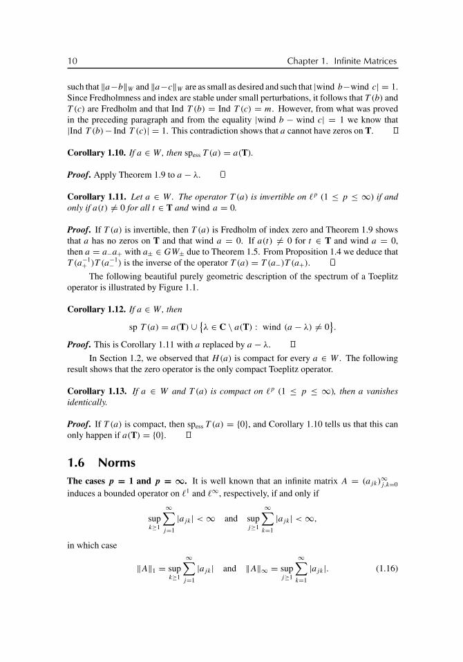
The following beautiful purely geometric description of the spectrum of a Toeplitzoperator is illustrated by Figure 1.1.

Corollary 1.12. If a ∈ W , then

sp T (a) = a(T) ∪ {λ ∈ C \ a(T) : wind (a − λ) �= 0

}.

Proof. This is Corollary 1.11 with a replaced by a − λ.

In Section 1.2, we observed that H(a) is compact for every a ∈ W . The followingresult shows that the zero operator is the only compact Toeplitz operator.

Corollary 1.13. If a ∈ W and T (a) is compact on �p (1 ≤ p ≤ ∞), then a vanishesidentically.

Proof. If T (a) is compact, then spess T (a) = {0}, and Corollary 1.10 tells us that this canonly happen if a(T) = {0}.

1.6 NormsThe cases p = 1 and p = ∞. It is well known that an infinite matrix A = (ajk)

∞j,k=0

induces a bounded operator on �1 and �∞, respectively, if and only if

supk≥1

∞∑j=1

|ajk| <∞ and supj≥1

∞∑k=1

|ajk| <∞,

in which case

‖A‖1 = supk≥1

∞∑j=1

|ajk| and ‖A‖∞ = supj≥1

∞∑k=1

|ajk|. (1.16)

buch72005/10/5page 11

�

�

�

�

�

�

�

�

1.6. Norms 11

−6 −4 −2 0 2 4 6 8−8

−6

−4

−2

0

2

4

6

−6 −4 −2 0 2 4 6 8−8

−6

−4

−2

0

2

4

6

Figure 1.1. The essential spectrum spess T (a) = a(T) on the left and the spectrumsp T (a) on the right.

This easily implies the following.

Theorem 1.14. If a ∈ W then ‖T (a)‖1 = ‖T (a)‖∞ = ‖a‖W .

The case p = 2. Let L2 := L2(T) be the usual Lebesgue space of complex-valued functionson T with the norm

‖f ‖2 :=(∫

T|f (t)|2 |dt |

2π

)1/2

=(∫ 2π

0|f (eiθ )|2 dθ

2π

)1/2

.

The set H 2 := H 2(T) := {f ∈ L2 : fn = 0 for n < 0} is a closed subspace of L2 andis referred to as the Hardy space of L2. Let P : L2 → H 2 be the orthogonal projection.Thus, if f ∈ L2 is given by

f (t) =∞∑

n=−∞fnt

n (t ∈ T),

then

(Pf )(t) =∞∑

n=0

fntn (t ∈ T).

The map

� : H 2 → �2, f �→ {fn}∞n=0 (1.17)

is a unitary operator of H 2 onto �2. It is not difficult to check that if a ∈ W , then �−1T (a)�

is the operator

�−1T (a)� : H 2 → H 2, f �→ P(af ), (1.18)

buch72005/10/5page 12

�

�

�

�

�

�

�

�


where (af )(t) := a(t)f (t). The observation (1.18) is in fact the key to the theory of Toeplitzoperators on �2. We here confine ourselves to the following consequence of (1.18).

Theorem 1.15. If a ∈ W then ‖T (a)‖2 = ‖a‖∞, where ‖a‖∞ := maxt∈T |a(t)|.

Proof. If f ∈ H 2, then ‖�−1T (a)�f ‖2 = ‖P(af )‖2 ≤ ‖af ‖2 ≤ ‖a‖∞‖f ‖2, whence‖T (a)‖2 = ‖�−1T (a)�‖2 ≤ ‖a‖∞. On the other hand, Corollary 1.12 implies that thespectral radius

rad T (a) = max{|λ| : λ ∈ sp T (a)

}is equal to ‖a‖∞. Because rad T (a) ≤ ‖T (a)‖2, it follows that ‖a‖∞ ≤ ‖T (a)‖2.

Other values of p. This case is more delicate, but one has at least two-sided estimates.

Proposition 1.16. If a ∈ W and 1 ≤ p ≤ ∞, then ‖a‖∞ ≤ ‖T (a)‖p ≤ ‖a‖W .

Proof. The inequality ‖T (a)‖p ≤ ‖a‖W results from Proposition 1.1, and the inequality‖a‖∞ ≤ ‖T (a)‖p is a consequence of Corollary 1.12 together with the estimate ‖a‖∞ =rad T (a) ≤ ‖T (a)‖p.

1.7 InversesLet b be a Laurent polynomial of the form (1.10). Suppose b(t) �= 0 for t ∈ T andwind b = 0. From Section 1.4 we know that b can be written in the form b = b−b+ with

b−(t) =r∏

j=1

(1− δj

t

), b+(t) = bs

s∏k=1

(t − μk), (1.19)

where δ := max(|δ1|, . . . , |δr |) < 1 and μ := min(|μ1|, . . . , |μs |) > 1. When provingCorollary 1.11, we observed that

T −1(b) = T (b−1+ )T (b−1

− ). (1.20)

From (1.19) we see that

b−1− (t) =

r∏j=1

(1+ δj

t+ δ2

j

t2+ · · ·

)=:

∞∑m=0

cm

tm,

b−1+ (t) = 1

bs

s∏k=1

(− 1

μk

) s∏k=1

(1+ t

μk

+ t2

μ2k

+ · · ·)=:

∞∑m=0

dmtm.

With the coefficients cm and dm, formula (1.20) takes the form

T −1(b) =

⎛⎜⎜⎝d0

d1 d0

d2 d1 d0

. . . . . . . . . . . .

⎞⎟⎟⎠⎛⎜⎜⎝

c0 c1 c2 . . .

c0 c1 . . .

c0 . . .

. . .

⎞⎟⎟⎠ . (1.21)

buch72005/10/5page 13

�

�

�

�

�

�

�

�

1.7. Inverses 13

Proposition 1.3 and (1.20) imply that

T −1(b) = T (b−1)−H(b−1+ )H (b−1

− ). (1.22)

Representation (1.20) gives us T −1(b) as the product of the lower triangular matrix T (b−1+ )

and the upper triangular matrix T (b−1− ), while (1.22) shows that T −1(b) is the difference of

the (in general full) Toeplitz matrix T (b−1) and the product H(b−1+ )H (b−1

− ) of two Hankelmatrices.

Let α be any number satisfying

0 < α < min

(log

1

δ, log μ

). (1.23)

Lemma 1.17. For every n ≥ 0,

| (b−1−

)−n| ≤

(min|z|=δ+ε

|b−(z)|)−1

(δ + ε)n (ε > 0), (1.24)

| (b−1+

)n| ≤

(min|z|=μ−ε

|b+(z)|)−1

(μ− ε)n (0 < ε < μ). (1.25)

Consequently, (b−1− )−n and (b−1

+ )n are O(e−αn) as n→∞.

Proof. Since 1/b−(z) is analytic for |z| > δ, we get

(b−1− )−n = 1

2πi

∫|z|=1

zn−1dz

b−(z)= 1

2πi

∫|z|=δ+ε

zn−1dz

b−(z)

and hence

|(b−1− )−n| ≤ 1

2π

(min|z|=δ+ε

|b−(z)|)−1

(δ + ε)n−12π(δ + ε),

which is (1.24). Estimate (1.25) can be verified analogously.

Proposition 1.18. For the j, k entry of T −1(b) we have the estimate[T −1(b)

]j,k= (

b−1)j−k+O

(e−α(j+k)

).

Proof. From (1.22) we see that∣∣∣[T −1(b)]j,k− (b−1)j−k

∣∣∣ = ∣∣∣∣∣∞∑

�=1

(b−1+ )j+�(b

−1− )−k−�

∣∣∣∣∣≤

( ∞∑�=1

|(b−1+ )j+�|2

∞∑�=1

|(b−1− )−k−�|2

)1/2

, (1.26)

and Lemma 1.17 implies that (1.26) is

O

⎛⎝( ∞∑�=1

e−2α(j+�)

)1/2⎞⎠ O

⎛⎝( ∞∑�=1

e−2α(k+�)

)1/2⎞⎠ = O(e−αj ) O(e−αk).

buch72005/10/5page 14

�

�

�

�

�

�

�

�


Given two sequences x = {xk} and y = {yk}, we set (x, y) =∑xkyk . The j, k entry

of T −1(b) is just (T −1(b)x, y) for x = ek and y = ej , where {en} is the standard basis of �2.The following useful observation evaluates (T −1(b)x, y) at another interesting pair (x, y).For z ∈ D, define wz ∈ �2 by (wz)n = zn (n ≥ 0).

Proposition 1.19. Let b = b−b+ with b± given by (1.19). Then for α, β ∈ D,

(T −1(b)wα, wβ) = 1

bs

1

1− αβ

r∏j=1

1

1− δjα

s∏k=1

1

β − μk

(1.27)

= 1

1− αβ

1

b−(1/α)b+(β). (1.28)

Proof. We have

(T −1(b)wα, wβ) = (T (b−1+ )T (b−1

− )wα, wβ) = (T (b−1− )wα, T (b

−1+ )wβ).

Define χn(t) := tn (t ∈ T). It is easily seen that, for |δ| < 1,

T −1(1− δχ−1)wα = T (1+ δχ−1 + δ2χ−2 + · · · )wα = 1

1− δαwα,

whence

T (b−1− )wα =

⎛⎝ r∏j=1

1

1− δjα

⎞⎠wα.

Analogously, if |μ| > 1,

T −1(χ−1 − μ)wβ = − 1

μT −1

(1− 1

μχ−1

)wβ = − 1

μ

1

1− μ−1βwβ = 1

β − μwβ,

which implies that

T (b−1+ )wβ = b

−1s

(s∏

k=1

1

β − μk

)wβ.

Consequently,

(T (b−1− )wα, T (b

−1+ )wβ) = 1

bs

r∏j=1

1

1− δjα

s∏k=1

1

β − μk

(wα, wβ).

As (wα, wβ) = 1/(1− αβ), we arrive at (1.27). Clearly, (1.28) is nothing but another wayof writing (1.27).

buch72005/10/5page 15

�

�

�

�

�

�

�

�

1.8. Eigenvalues and Eigenvectors 15

1.8 Eigenvalues and EigenvectorsLet b be a Laurent polynomial. In this section we study the problem of finding the λ ∈sp T (b) for which there exist nonzero x ∈ �p such that T (b)x = λx. These λ are calledeigenvalues of T (b) on �p, and the corresponding x’s are referred to as eigenelements oreigenvectors (which sounds much better). Since T (b) − λI = T (b − λ), our problem isequivalent to the question of when a Toeplitz operator has a nontrivial kernel. Throughoutthis section we assume that b is not constant on the unit circle T.

Outside the essential spectrum. For a point λ ∈ C \ b(T), we denote by wind (b, λ) thewinding number of b about λ, that is, wind (b, λ) := wind (b − λ). A sequence {xn}∞n=0is said to be exponentially decaying if there are C ∈ (0,∞) and γ ∈ (0,∞) such that|xn| ≤ Ce−γ n for all n ≥ 0.

Proposition 1.20. Let 1 ≤ p ≤ ∞. A point λ /∈ b(T) is an eigenvalue of T (b) as anoperator on �p if and only if wind (b, λ) = −m < 0, in which case Ker (T (b) − λI) hasthe dimension m and each eigenvector is exponentially decaying.

Proof. From Theorem 1.8 (or simply from (1.13)) we get a Wiener-Hopf factorizationb(t) − λ = b−(t)t−mb+(t). Proposition 1.4 implies that T (b − λ) decomposes into theproduct T (b−)T (χ−m)T (b+) and that the operators T (b±) are invertible, the inverses beingT (b−1

± ). Thus, x ∈ Ker T (b − λ) if and only if T (χ−m)T (b+)x = 0. If m ≤ 0, this isequivalent to the equation T (b+)x = 0 and hence to the equality x = 0. So let m > 0.We denote by ej ∈ �p the sequence given by (ej )k = 1 for k = j and (ej )k = 0 fork �= j . Clearly, T (χ−m)T (b+)x = 0 if and only if T (b+)x belongs to the linear hulllin {e0, . . . , em−1} of e0, . . . , em−1. Consequently,

Ker T (b − λ) = lin {T (b−1+ )e0, . . . , T (b−1

+ )em−1}.This shows that dim Ker T (b−λ) = m, and from Lemma 1.17 we deduce that the sequencesin Ker T (b − λ) are exponentially decaying.

Inside the essential spectrum. Things are a little bit more complicated for points λ ∈ b(T).In that case b − λ has zeros on T. For τ ∈ T, we define the function ξτ by

ξτ (t) = 1− τ

t(t ∈ T).

Notice that ξτ has a single zero on T and that T (ξτ ) is the upper triangular matrix

T (ξτ ) =

⎛⎜⎜⎝1 −τ 0 . . .

0 1 −τ . . .

0 0 1 . . .

. . . . . . . . . . . .

⎞⎟⎟⎠ .

Lemma 1.21. Let τ1, . . . , τ� be distinct points on T and let α1, . . . , α� be positive integers.Then

Ker T(ξα1τ1

. . . ξα�

τ�

) = {0} on �p (1 ≤ p <∞) (1.29)

buch72005/10/5page 16

�

�

�

�

�

�

�

�


and

Ker T(ξα1τ1

. . . ξα�

τ�

) = lin {wτ1 , . . . , wτ�} on �∞, (1.30)

where (wτ )n := 1/τn.

Proof. Put ξ = ξα1τ1

. . . ξα�τ�

and write

ξ(t) = a0 + a11

t+ a2

1

t2+ · · · + aN

1

tN.

The equation T (ξ)x = 0 is the difference equation

a0xn + a1xn+1 + · · · + aNxn+N = 0 (n ≥ 0),

which is satisfied if and only if

xn =α1−1∑k=0

γ(1)k

nk

τ n1

+ · · · +α�−1∑k=0

γ(�)k

nk

τ n�

(1.31)

with complex numbers γ(j)

k . The sequence given by (1.31) belongs to �p (1 ≤ p < ∞) ifand only if it is identically zero, which proves (1.29), and it is in �∞ if and only if it is ofthe form

xn = γ(1)0

1

τn1

+ · · · + γ(�)0

1

τn�

,

which gives (1.30).

Given λ ∈ b(T), we denote the distinct zeros of b − λ on T by τ1, . . . , τ� and theirmultiplicities by α1, . . . , α�. We extract the zeros by “anti-analytic” linear factors, that is,we write b − λ in the form

b(t)− λ =�∏

j=1

(1− τj

t

)αj

c(t), (1.32)

where c(t) �= 0 for t ∈ T.

Proposition 1.22. Let 1 ≤ p < ∞. Suppose λ ∈ b(T) and write b − λ in the form (1.32).Then λ is an eigenvalue of the operator T (b) on �p if and only if wind c = −m < 0, inwhich case Ker (T (b) − λI) is of the dimension m and all eigenvectors are exponentiallydecaying.

Proof. By Proposition 1.4,

T (b − λ) =�∏

j=1

[T (ξτj)]αj T (c). (1.33)

buch72005/10/5page 17

�

�

�

�

�

�

�

�


From (1.29) we see that Ker T (b−λ) = Ker T (c), and Proposition 1.20 therefore gives theassertion.

We now turn to the case p = ∞. A sequence {xn}∞n=0 is called extended if

lim supn→∞

|xn| > 0.

Proposition 1.23. Let λ ∈ b(T) and write b−λ in the form (1.32). Then λ is an eigenvalue ofT (b) on �∞ if and only if wind c = −m < �. In that case the dimension of Ker (T (b)−λI)

is m+�. There is a basis in Ker (T (b)−λI) whose elements enjoy the following properties:(a) if m > 0, then m elements of the basis decay exponentially and � elements have

zeros in the first m places and are extended;(b) if m ≤ 0, then all the �− |m| elements of the basis are extended.

Proof. Combining (1.30) and (1.33), we see that T (b − λ)x = 0 if and only if there arecomplex numbers γj such that

T (c)x =�∑

j=1

γjwτj. (1.34)

Let c = c−χ−mc+ be a Wiener-Hopf factorization of c. It can be readily checked thatT (c−1

− )wτ = c−1− (1/τ)wτ . Thus, setting δj = γj c

−1− (1/τj ), we can rewrite (1.34) in the

form

T (χ−m)T (c+)x =�∑

j=1

δjwτj. (1.35)

If m ≥ 0, then (1.35) holds if and only if

T (c+)x ∈ lin {e0, . . . , em−1, T (χm)wτ1 , . . . , T (χm)wτ�},

which is equivalent to the requirement that x be in

lin {T (c−1+ )e0, . . . , T (c−1

+ )em−1, T (χm)T (c−1+ )wτ1 , . . . , T (χm)T (c−1

+ )wτ�}.

The sequences T (c−1+ )ej decay exponentially (Lemma 1.17), and since

[T (c−1+ )wτ ]n = 1

τn

n∑k=0

(c−1+ )kτ

k,

it follows that the sequences T (c−1+ )wτj

are extended. This completes the proof in the casem ≥ 0.

Let now m < 0. In that case (1.35) is satisfied if and only if

�∑j=1

δj (1/τj )n = 0 for n = 0, 1, . . . , |m| − 1 (1.36)

buch72005/10/5page 18

�

�

�

�

�

�

�

�


and

x =�∑

j=1

δjT (c−1+ )T (χ−|m|)wτj

. (1.37)

Equations (1.36) are a Vandermonde system for the δj ’s. If |m| ≥ �, then (1.36) has onlythe trivial solution. If |m| < �, we can choose δ1, . . . , δ�−|m| arbitrarily. The numbersδ�−|m|+1, . . . , δ� are then uniquely determined. This shows that the set of all x of the form(1.37) has the dimension �− |m| and that all nonzero x in this set are extended.

In geometric terms, the winding number of the function c in (1.32) can be determinedas follows. Choose a number � > 1 and consider the function b� defined by b�(t) = b(�t)

(t ∈ T). If � is sufficiently close to 1, then b�−λ has no zeros on T and hence wind (b�, λ)

is well defined.

Proposition 1.24. We have wind c = lim�→1+0

wind (b�, λ).

Proof. Let c�(t) := c(�t). From (1.32) we obtain b�(t) − λ = ∏�j=1 (1 − τj

�t)αj c�(t),

whence wind (b�, λ) = wind c�. Since wind c� converges to wind c as � → 1, we arrive atthe assertion.

Frequently, the following observation is very useful.

Proposition 1.25. Let λ ∈ b(T) and suppose � is a connected component of C \ b(T)

whose boundary contains λ. If wind (b, z) = κ for z ∈ �, then wind c ≥ κ.

Proof. For z ∈ �, we have

b(t)− z = bst−r

r+κ∏j=1

(t − δj (z))

s−κ∏k=1

(t − μk(z))

with |δj (z)| < 1 and |μk(z)| > 1. Now let z ∈ � approach λ ∈ ∂�. The some of the δj (z),say δ1(z), . . . , δm(z), move onto the unit circle, while the remaining δj (z) stay in the openunit disk. Analogously, some of the μk(z), say μ1(z), . . . , μ�(z), attain modulus 1, whereasthe remaining μk(z) keep modulus greater than 1. We can write b(t)− λ as

bst−r

m∏j=1

(t − δj (λ))

r+κ∏j=m+1

(t − δj (λ))

�∏k=1

(t − μk(λ))

s−κ∏k=�+1

(t − μk(λ)).

The zeros of b� − λ are δj (λ)/� and μk(λ)/�. If � > 1, then |δj (λ)| < 1 for all j . If, inaddition, � > 1 is sufficiently close to 1, then |μk(λ)/�| > 1 for k = �+ 1, . . . , s − κ and|μk(λ)/�| < 1 for k = 1, . . . , �. The result is that

lim�→1+0

wind (b� − λ) = −r + (r + κ)+ � = κ + � ≥ κ.

From Proposition 1.24 we so obtain that wind c ≥ κ.

buch72005/10/5page 19

�

�

�

�

�

�

�

�


Corollary 1.26. If λ lies on the boundary of a connected component � of C \ b(T) suchthat wind (b, z) ≥ 0 for z ∈ �, then λ cannot be an eigenvalue of T (b) on �p (1 ≤ p <∞).

Proof. Immediate from Propositions 1.22 and 1.25.

Corollary 1.27. If b is a real-valued Laurent polynomial, then T (b) as an operator on �p

(1 ≤ p <∞) has no eigenvalues.

Proof. This is a straightforward consequence of Corollary 1.26. Here is an alternativeproof. Let λ ∈ b(T) and write b(t)−λ = br t

−r∏2r

j=1(t−zj ). Since b(t)−λ is real valued,

passage to the complex conjugate gives b(t)− λ = br t−r

∏2rj=1(t − 1/ zj ). Thus, if b − λ

has � ≥ 1 distinct zeros τ1, . . . , τ� on T and n ≥ 0 distinct zeros μ1, . . . , μn of modulusgreater than 1, then

b(t)− λ = br t−r

n∏j=1

[(t − μj)(t − 1/ μj )]βj

�∏j=1

(t − τj )αj =

�∏j=1

(1− τj

t

)αj

c(t)

with

c(t) = br t−r tα1+···+α�

n∏j=1

[(t − μj)(t − 1/ μj )]βj .

Clearly, wind c = −r+α1+· · ·+α�+β1+· · ·+βn. Since α1+· · ·+α�+2β1+· · ·+2βn = 2r

and αj ≥ 1 for all j , we get β1 + · · · + βn < r and thus wind c = r − β1 − · · · − βn > 0.The assertion now follows from Proposition 1.22.

Example 1.28. We remark that Corollary 1.27 is not true for p = ∞: the sequence{1, 0,−1, 0, 1, 0,−1, 0, . . . } is obviously in the kernel of the operator

T (χ−1 + χ1) =

⎛⎜⎜⎜⎜⎝0 1 0 0 . . .

1 0 1 0 . . .

0 1 0 1 . . .

0 0 1 0 . . .

. . . . . . . . . . . . . . .

⎞⎟⎟⎟⎟⎠ .

For this operator, things are as follows. The symbol is b(t) = t−1 + t and hence sp T (b) =b(T) = [−2, 2]. For λ ∈ [−2, 2],

b(t)− λ =(

1− τ1(λ)

t

)(1− τ2(λ)

t

)t,

where τ1(λ), τ2(λ) ∈ T are given by

τ1,2(λ) = λ

2± i

√1− λ2

4.

Thus, if λ ∈ (−2, 2), then Proposition 1.23 (with wind c = 1 and � = 2) implies thatT (b)− λI has a one-dimensional kernel in �∞ whose nonzero elements are extended, and

buch72005/10/5page 20

�

�

�

�

�

�

�

�


if λ ∈ {−2, 2}, then Proposition 1.23 (with wind c = 1 and � = 1) shows that the kernel ofT (b)− λI in �∞ is trivial.

Example 1.29. Let b(t) = (1+ 1/t)3. The image b(T) is the solid curve in the left pictureof Figure 1.2; this curve is traced out in the clockwise direction. The curve intersectsitself at the point −1. We see that C \ b(T) has two bounded connected components �1

and �2 with wind (b, λ) = −1 for λ ∈ �1 and wind (b, λ) = −2 for λ ∈ �2. Thus,sp T (b) = �1 ∪�2 ∪ b(T).

By Proposition 1.20, the points in �1 ∪ �2 are eigenvalues. Looking at Figure 1.2and using Proposition 1.24, we see that wind c = −1 for the points on the two smallopen arcs of b(T) that join 0 and −1. Thus, by virtue of Propositions 1.22 and 1.23, thesepoints are also eigenvalues. The points of b(T) which are boundary points of the unboundedconnected component of C\b(T), including the point−1, are not eigenvalues if 1 ≤ p <∞(Corollary 1.26), but they are eigenvalues if p = ∞, because wind c = 0 (Propositions 1.23and 1.24). Finally, for λ = 0 we have � = 1, and the right picture of Figure 1.2 reveals thatwind c = 0. Consequently, λ = 0 is not an eigenvalue if 1 ≤ p < ∞ (Proposition 1.22)and is an eigenvalue if p = ∞ (Proposition 1.23).

origin +

Figure 1.2. The curves b(T) (solid) and b�(T) with � = 1.05 (dotted). Both curvesare traced out clockwise. The right picture is a close-up (with a magnification about 4300)of the left picture in a neighborhood of the origin, which is marked by +.

Remark 1.30. Let b be a real-valued Laurent polynomial and suppose λ is a point in b(T).We know from Corollary 1.27 that Ker T (b − λ) = {0} in �p (1 ≤ p < ∞). This impliesthat if 1 < p < ∞, then the range Im T (b − λ) is not closed but dense in �p. In otherwords, T (b) has no residual spectrum on �p for 1 < p < ∞. However, the polynomialb = χ−1+χ1 is an example of a symbol for which Ker T (b) �= {0} in �∞ and thus Im T (b)

is not dense in �1. Consequently, there are b’s such that T (b) has a residual spectrum on �1.

buch72005/10/5page 21

�

�

�

�

�

�

�

�

1.9. Selfadjoint Operators 21

1.9 Selfadjoint OperatorsWe now consider Toeplitz operators on the space �2. Obviously, T (b) is selfadjoint if andonly if bn = b−n for all n, that is, if and only if b is real valued. Thus, let

b(eix) =s∑

k=−s

bkeikx = b0 +

s∑n=1

(an cos nx + cn sin nx),

where b0, an, cn are real numbers.

The resolution of the identity. Let A be a bounded selfadjoint operator on the space �2.Then the operator f (A) is well defined for every bounded Borel function f on R. Forλ ∈ R, put E(λ) = χ(−∞,λ](A), where χ(−∞,λ] is the characteristic function of (−∞, λ].The family {E(λ)}λ∈R is called the resolution of the identity for A. Stone’s formula statesthat

1

2(E(λ+ 0)+ E(λ− 0))x

= limε→0+0

1

2πi

∫ λ

−∞

((A− (λ+ iε)I )−1 − (A− (λ− iε)I )−1

)x dλ (1.38)

for every x ∈ �2. Let �2pp, �

2ac, �

2sing denote the set of all x ∈ �2 for which the measure dx(λ) :=

d(E(λ)x, x) is a pure point measure, is absolutely continuous with respect to Lebesguemeasure, and is singular continuous with respect to Lebesgue measure, respectively. Thesets �2

pp, �2ac, �

2sing are closed subspaces of �2 whose orthogonal sum is all of �2. Moreover,

each of the spaces �2pp, �

2ac, �

2sing is an invariant subspace of A. The spectra of the restrictions

A|�2ac and A|�2

sing are referred to as the absolutely continuous spectrum and the singularcontinuous spectrum of A, respectively. The point spectrum of A is defined as the set of theeigenvalues of A (and not as the spectrum of the restriction A|�2

pp). It is well known that thespectrum of A is the union of the absolutely continuous spectrum, the singular continuousspectrum, and the closure of the point spectrum.

The spectrum of T (b) is the line segment b(T) =: [m, M]. Corollary 1.27 tells usthat the point spectrum of T (b) is empty unless b is a constant. As the following theoremshows, the singular continuous spectrum is also empty.

Theorem 1.31 (Rosenblum). The spectrum of a Toeplitz operator generated by a real-valued nonconstant Laurent polynomial is purely absolutely continuous.

Proof. Let b be a real-valued nonconstant Laurent polynomial. We may without loss ofgenerality assume that the highest coefficient bs is 1. Fix λ ∈ R and ε > 0, and putz = λ+ iε. As in Section 1.4, we can write

b(t)− z =∏(

1− δj

t

)∏(t − μj),

where |δj | = |δj (z)| < 1 and |μj | = |μj(z)| > 1. Passing to the complex conjugate, we

buch72005/10/5page 22

�

�

�

�

�

�

�

�


get

b(t)− z =∏(

1− 1

μj t

)∏(t − 1

δj

).

Proposition 1.19 now implies that, for α ∈ D,

(T −1(b − z)wα, wα) = 1

f (z)

1

1− |α|2 , (T −1(b − z)wα, wα) = 1

f (z)

1

1− |α|2 ,

where f (z) :=∏(1− δjα)

∏(α − μj). We have∣∣∣∣ 1

f (z)− 1

f (z)

∣∣∣∣ = 2

∣∣∣∣ Im f (z)

|f (z)|2∣∣∣∣ ≤ 2

|f (z)| =2∏ |1− δjα|∏ |α − μj | ≤

2

(1− |α|)2s,

because |1− δjα| ≥ 1− |α| and |α−μj | ≥ 1− |α| for all j . Since E(λ− 0) = E(λ+ 0),formula (1.38) gives

|(E(λ2)wα, wα)− (E(λ1)wα, wα)| ≤ 1

2π

∫ λ2

λ1

2

(1− |α|)2sdλ,

which shows that the function λ �→ (E(λ)wα, wα) is absolutely continuous for each α ∈ D.It follows that wα ∈ �2

ac for each α ∈ D, and as the linear hull of the set {wα}α∈D is dense in�2, we arrive at the conclusion that �2

ac = �2, which is the assertion.

The problem of diagonalizing selfadjoint bounded Toeplitz operators is solved. Moreor less explicit formulas can be found in [227], [228], [229], and [288]. We here confineourselves to a few simple observations.

Chebyshev polynomials. We denote by {Un}∞n=0 the normalized Chebyshev polynomialsof the second kind:

Un(cos θ) =√

2

π

sin(n+ 1)θ

sin θ.

The polynomials {Un}∞n=0 constitute an orthonormal basis in the Hilbert space L2((−1, 1),√1− λ2) =: L2(σ ), ∫ 1

−1Uj(λ)Uk(λ)

√1− λ2 dλ = δjk,

and they satisfy the identities

λUn(λ) = 1

2Un+1(λ)+ 1

2Un−1(λ), U−1(λ) := 0. (1.39)

For α ∈ T, we define Vα : �2 → L2(σ ) by

(Vαx)(λ) =∞∑

n=0

xnαnUn(λ), λ ∈ (−1, 1).

buch72005/10/5page 23

�

�

�

�

�

�

�

�


Clearly, Vα is unitary and V −1α : L2(σ )→ �2 acts by the rule

(V −1α f )n = 1

αn

∫ 1

−1f (λ)Un(λ)

√1− λ2 dλ, n ≥ 0.

We denote by Mf (λ) the operator of multiplication by the function f (λ) on L2(σ ).

Proposition 1.32. Let

b(eix) = b1e−ix + b0 + b1e

ix = b0 + a1 cos x + c1 sin x

be a real valued trinomial. Put

α =√

b1

b1=

√a1 + ic1

a1 − ic1, β = 2|b1| = 1

2

√a2

1 + c21.

Then T (b) = V −1α Mb0+βλVα .

Proof. Using (1.39) and the orthonormality of the polynomials Un we obtain

(V −1α MλVαx)n = 1

αn

∫ 1

−1λ(Vαx)(λ)Un(λ)

√1− λ2 dλ

= 1

αn

∞∑k=0

xkαk

∫ 1

−1λUk(λ)Un(λ)

√1− λ2 dλ

= 1

αn

∞∑k=0

xkαk

∫ 1

−1

(1

2Uk(λ)Un+1(λ)+ 1

2Uk(λ)Un−1(λ)

)√1− λ2 dλ

= 1

αn

(xn+1

αn+1

2+ xn−1

αn−1

2

)= α

2xn+1 + 1

2αxn−1,

where x−1 := 0. Equivalently,

V −1α MλVα = T

(α

2χ−1 + 1

2αχ1

).

This implies that V −1α Mb0+2|b1|λVα is the Toeplitz operator with the symbol

b0 +√

b1

b1|b1|χ−1 +

√b1

b1|b1|χ1 = b0 + b1χ−1 + b1χ1.

In particular,

T (cos x) := T

(1

2χ−1 + 1

2χ1

)= V −1

1 MλV1, (1.40)

T (sin x) := T

(i

2χ1 − i

2χ−1

)= V −1

i MλVi. (1.41)

buch72005/10/5page 24

�

�

�

�

�

�

�

�


Diagonalization of symmetric and skewsymmetric Toeplitz matrices. The polynomials

g(x) = b0 +s∑

n=1

an cos nx and u(x) =s∑

n=1

cn sin nx

generate symmetric (A� = A) and skewsymmetric (A� = −A) Toeplitz matrices, respec-tively. From identities (1.39) we infer that

λ2Un(λ) = 1

4Un+2(λ)+ 1

2Un(λ)+ 1

4Un−2(λ),

λ3Un(λ) = 1

8Un+3(λ)+ 3

8Un+1(λ)+ 3

8Un−1(λ)+ 1

8Un−3(λ),

and so on, where U−2(λ) = U−3(λ) = · · · = 0. Consequently, as in the proof of Proposition1.32,

T

(1

2+ 1

4cos 2x

)= T

(1

4χ−2 + 1

2χ0 + 1

4χ2

)= V −1

1 Mλ2V1,

T

(3

8cos x + 1

8cos 3x

)= T

(1

8χ−3 + 3

8χ−1 + 3

8χ1 + 1

8χ3

)= V −1

1 Mλ3V1,

etc. This shows that we can find coefficients γ0, γ1, . . . , γs such that

T

(b0 +

s∑n=1

an cos nx

)= V −1

1 Mγ0+γ1λ+···+γsλs V1.

One can diagonalize the skewsymmetric matrices T (u) analogously.

Resolution of the identity for Toeplitz operators. Let A be a bounded selfadjoint operatoron �2 and suppose we have a unitary operator V such that V AV −1 is multiplication by λ onL2(σ ) := L2((−1, 1),

√1− λ2). Then the resolution of the identity for A can be computed

from the formula E(λ) = V Mχ(−∞,λ]V−1. Clearly, we can think of E(λ) as an infinite matrix

(Ejk(λ))∞j,k=0.

Proposition 1.33. The resolution of the identity for T (cos x) = T ( 12χ−1 + 1

2χ1) is givenby E(λ) = 0 for λ ∈ (−∞,−1], E(λ) = I for λ ∈ [1,∞), and

Ejk(λ) =

⎧⎪⎪⎪⎨⎪⎪⎪⎩1

π

(sin(j + k + 2)θ

j + k + 2− sin(j − k)θ

j − k

)if j �= k

1

π

(sin(2j + 2)θ

2j + 2− θ + π

)if j = k

with θ = arccos λ for λ ∈ (−1, 1).

Proof. It suffices to consider λ in (−1, 1). Let en be the nth element of the standard basis

buch72005/10/5page 25

�

�

�

�

�

�

�

�


of �2. By virtue of (1.40),

Ejk(λ) = (E(λ)ek, ej ) = (V −11 Mχ(−∞,λ)

V1ek, ej )

= (Mχ(−∞,λ)V1ek, V1ej ) = (Mχ(−∞,λ)

Uk, Uj )

=∫ λ

−1Uk(μ)Uj (μ)

√1− μ2 dμ

= 2

π

∫ π

θ

sin(k + 1)ϕ

sin ϕ

sin(j + 1)ϕ

sin ϕsin2 ϕ dϕ

= 1

π

∫ π

θ

[cos(j − k)ϕ − cos(j + k + 2)ϕ] dϕ,

which implies the assertion.

From (1.40) we also deduce that if f is any continuous function on [−1, 1], then thej, k entry of f (T (cos x)) is

[f (T (cos x))]jk = (V −11 Mf (λ)V1ek, ej ) = (Mf (λ)Uk, Uj )

=∫ 1

−1f (λ)Uk(λ)Uj (λ)

√1− λ2 dλ

= 2

π

∫ π

θ

f (cos θ)sin(k + 1)θ

sin θ

sin(j + 1)θ

sin θsin2 θ dθ

= 1

π

∫ π

θ

f (cos θ)[cos(j − k)θ − cos(j + k + 2)θ ] dθ.

For example, the nonnegative square root of

T (2− 2 cos x) =

⎛⎜⎜⎝2 −1 0 . . .

−1 2 −1 . . .

0 −1 2 . . .

. . . . . . . . . . . .

⎞⎟⎟⎠has j, k entry

1

π

∫ π

θ

√2− 2 cos θ [cos(j − k)θ − cos(j + k + 2)θ ] dθ

= 2

π

∫ π

θ

(sin

θ

2

)[cos(j − k)θ − cos(j + k + 2)θ ] dθ

= 1

π

∫ 1

−1

[sin

(j − k + 1

2

)θ − sin

(j − k − 1

2

)θ

− sin

(j + k + 2+ 1

2

)θ + sin

(j + k + 2− 1

2

)θ

]dθ

= 1

π

(1

j − k + 12

− 1

j − k − 12

+ 1

j + k + 2+ 12

− 1

j + k + 2− 12

),

and this equals

4

π

(1

4(j + k + 2)2 + 1− 1

4(j − k)2 + 1

).

buch72005/10/5page 26

�

�

�

�

�

�

�

�


Exercises

1. (a) Find a function a ∈ L∞(T) whose Fourier coefficients an (n ∈ Z) are justan = 1/(n+ 1/2).

(b) Show that the infinite Toeplitz matrix⎛⎜⎜⎜⎝1 − 1

2 − 13 . . .

12 1 − 1

2 . . .13

12 1 . . .

. . . . . . . . . . . .

⎞⎟⎟⎟⎠induces a bounded operator on �2 but not on �1.

(c) Show that the infinite Toeplitz matrix⎛⎜⎜⎜⎝1 1

213 . . .

12 1 1

2 . . .13

12 1 . . .

. . . . . . . . . . . .

⎞⎟⎟⎟⎠does not generate a bounded operator on �2.

(d) Show that the infinite upper-triangular Toeplitz matrix⎛⎜⎜⎜⎝1 1

213 . . .

1 12 . . .

1 . . .

. . .

⎞⎟⎟⎟⎠does not define a bounded operator on �2 but that the infinite Hankel matrix⎛⎜⎜⎜⎝

1 12

13 . . .

12

13 . . . . . .

13 . . . . . . . . .

. . . . . . . . . . . .

⎞⎟⎟⎟⎠is the matrix of a bounded operator on �2.

2. Prove that H(ab) = H(a) T (b)+ T (a) H(b) for all a, b ∈ W .

3. Find a Wiener-Hopf factorization of 6t − 41+ 31t−1 − 6t−2.

4. Let b1, . . . , bm ∈ P+ have no common zero on T. Prove that there are c1, . . . , cm ∈ W

such that T (c1)T (b1) + · · · + T (cm)T (bm) = I . Can one choose the c1, . . . , cm asrational functions without poles on T?

5. Let b(t) = 1+ 2t + γ t3. Show that there is no γ ∈ C for which T (b) is invertible.

buch72005/10/5page 27

�

�

�

�

�

�

�

�

Exercises 27

6. Let

b(t) = det

⎛⎜⎜⎜⎜⎝2 1 0 0 01 2 1 0 00 1 2 1 00 0 1 2 11 t t2 t3 t4

⎞⎟⎟⎟⎟⎠ .

Show that b has no zeros on T and that wind b = 4. Try to prove the analogue of thisif the 5× 5 determinant is replaced by an n× n determinant in the obvious way.

7. Let b(t) = 4+∑5j=−5 t j . Show that T (b) is invertible.

8. Let b be a Laurent polynomial and 1 ≤ p ≤ ∞. Show that T (b) : �p → �p hasclosed range if and only if either b is identically zero or b has no zeros on T.

9. Let bn(t) = 1+ 12 (t + t−1)+ 1

3 (t2 + t−2)+ · · · + 1n(tn + t−n). Show that

2 log n+ 0.1544 ≤ ‖T (bn)‖4 ≤ 2 log n+ 0.1545

for all sufficiently large n.

10. Prove that ‖T (a) + K‖p ≥ ‖T (a)‖p for every a ∈ W and every compact operatoron �p (1 ≤ p ≤ ∞). Deduce that the zero operator is the only compact Toeplitzoperator.

11. Prove that ‖T n(a)‖2 = ‖T (an)‖2 for every a ∈ W .

12. Show that there exist Laurent polynomialsb such that‖H(b)‖2 < ‖b‖∞ and‖H(b)‖1 <

‖b‖W .

13. For b =∑j bjχj ∈ P , define

Snb =∑

|j |≤n−1

bjχj , σnb = 1

n(S1b + · · · + Snb).

Prove that always ‖T (σnb)‖2 ≤ ‖T (b)‖2 but that there exist b and n such that‖T (Snb)‖2 > 100 ‖T (b)‖2.

14. Show that if a ∈ W and T (a) is a unitary operator on �2, then a is a unimodularconstant.

15. Let B = (bjk)∞j,k=1 with b23 = b32 = −1 and bjk = 0 otherwise. Show that the

operator T (χ−1 + χ1)+ B ∈ B(�p) (1 ≤ p ≤ ∞) has eigenvalues in (−2, 2).

16. Let A = T (χ−1 + χ1) + diag (vj )∞j=1. Show that if vj = o(1/j), then A ∈ B(�2)

has at most finitely many eigenvalues in each segment [α, β] ⊂ (−2, 2) and that ifvj = o(1/j 1+ε) with some ε > 0, then the only possible eigenvalues of A ∈ B(�2)are −2 and 2.

buch72005/10/5page 28

�

�

�

�

�

�

�

�


17. Show that the positive square root of T (2+2 cos x) is the Toeplitz-plus-Hankel matrix

4

π

((−1)j−k+1

(2j − 2k − 2)(2j − 2k + 1)+ (−1)j+k+2

(2j + 2k + 3)(2j + 2k + 5)

)∞j,k=0

.

Notes

In his 1911 paper [267], Otto Toeplitz considered doubly infinite matrices of the form(aj−k)

∞j=−∞ and proved that the spectrum of the corresponding operator on �2(Z) is just the

curve { ∞∑k=−∞

aktk : t ∈ T

}.

The matrices L(a) := (aj−k)∞j=−∞ are nowadays called Laurent matrices. In a footnote

of [267], Toeplitz established that the simply infinite matrix (aj−k)∞j=0 induces a bounded

operator on �2(Z+) if and only if the doubly infinite matrix (aj−k)∞j=−∞ generates a bounded

operator on �2(Z). This is why the matrices (aj−k)∞j=0 now bear his name.

The material of Sections 1.1 to 1.7 is standard. The books [71] and [130] may serve asintroductions to the basic phenomena in connection with infinite Toeplitz matrices. A nicesource is also [150]. In [25], infinite systems with a banded Toeplitz matrix T (a) are treatedwith the tools of the theory of difference equations; in this book, we find formulas for theentries of the inverses in terms of the zeros of a(z) (z ∈ C) and solvability criteria in thespaces of sequences x = {xn}∞n=1 subject to the condition xn = O(�n). Advanced topics inthe theory of infinite Toeplitz matrices (= Toeplitz operators) are treated in the monographs[70], [103], [195], [196]. The standard texts on Hankel matrices are [196], [201], [204],[213].

Full proofs of Theorems 1.5, 1.6, 1.7 can be found in [103] or [230], for example.Theorem 1.8 as it is stated is due to Mark Krein [184]. The method of Wiener-Hopffactorization was introduced by N. Wiener and E. Hopf in 1931. What we call Wiener-Hopffactorization has its origin in the work of Gakhov [123], although the basic idea (in the case ofvanishing winding number) was already employed by Plemelj [205]. Mark Krein [184] wasthe first to understand the operator theoretic essence and the Banach algebraic backgroundof Wiener-Hopf factorization and to present the method in a crystal-clear manner.

The results of Section 1.5 are also due to Krein [184]. However, it had been known along time before that T (a) is Fredholm of index−wind a whenever a has no zeros on T; thisinsight is more or less explicit in works by F. Noether, S. G. Mikhlin, N. I. Muskhelishvili,F. D. Gakhov, V. V. Ivanov, A. P. Calderón, F. Spitzer, H. Widom, A. Devinatz, G. Fichera,and certainly others. Moreover, in 1952, Israel Gohberg [128] had already proved that T (a)

is Fredholm if and only if a has no zeros on T. From this result it is only a small step (fromthe present-day understanding of the matter) to the formula Ind T (a) = −wind a.

Section 1.8 is based on known results of [129], [130], [184].Rosenblum’s papers [226], [227], [228] are the classics on selfadjoint Toeplitz oper-

ators. The monograph [229] contains very readable material on the topic. In these works

buch72005/10/5page 29

�

�

�

�

�

�

�

�

Notes 29

one can also find precise references to previous work on selfadjoint Toeplitz operators. Forexample, in [229] it is pointed out that the diagonalization (1.40) was carried out by Hilbert(1912) and Hellinger (1941). Proposition 1.19 is from [81] and [226] and Theorem 1.31was established in [226]. The results around Proposition 1.32 are special cases of moregeneral results in [227], [228]. Part of Rosenblum’s theory was simplified and generalizedby Vreugdenhil [288]. We took Proposition 1.33 and the example following after it from[288].

Exercises 5 and 6 are from [208]. Exercises 15 and 16 are results of the papers [182],[183]. Actually, these two papers are devoted to the following more general problem: Ifλ is not an eigenvalue for T (b) ∈ B(�p), for which perturbations B ∈ B(�p) is λ not aneigenvalue of T (b)+B? In [183] it is in particular proved that if B = (bjk)

∞j,k=1 is such that

bjk = 0 for j > k and (j 1+εbjk)∞j,k=1 induces a bounded operator on �p (1 ≤ p <∞), then

the interval (−2, 2) contains no eigevalues of T (χ−1+χ1)+B. As Exercise 15 shows, therequirement that B be upper-triangular is essential. A solution to Exercise 17 is in [288].

buch72005/10/5page 30

�

�

�

�

�

�

�

�

buch72005/10/5page 31

�

�

�

�

�

�

�

�

Chapter 2

Determinants

In this chapter, the main actors of this book enter the scene: finite Toeplitz matrices. For a

in the Wiener algebra W and n ∈ {1, 2, 3, . . . }, we define the n× n Toeplitz matrix Tn(a)

as the principal n× n section of T (a), that is, by

Tn(a) := (aj−k)nj,k=1 =

⎛⎜⎜⎜⎝a0 a−1 . . . a−(n−1)

a1 a0 . . . a−(n−2)

......

. . ....

an−1 an−2 . . . a0

⎞⎟⎟⎟⎠ . (2.1)

If a finite Toeplitz matrix is a circulant matrix, then nearly every piece of information on itsspectral properties is explicitly available. We also provide formulas for the eigenvalues andeigenvectors of tridiagonal Toeplitz matrices. Things are significantly more complicatedfor general Toeplitz matrices.

The focus of this chapter is on the determinants Dn(a) := det Tn(a). We establishseveral exact and asymptotic formulas for these determinants, including the Szegö-Widomlimit theorem and the Geronimo-Case-Borodin-Okounkov formula. Clearly, nowadaysnobody would determine the eigenvalues of Tn(a) by computing the zeros of the polynomialDn(a − λ) = det(Tn(a)− λI) = det Tn(a − λ). However, the results of Chapter 11 on theasymptotic distribution of the eigenvalues of Tn(a) in the limit n → ∞ are heavily basedon consideration of determinants and, independently of eigenvalues, Toeplitz determinantsare a hot topic in statistical physics.

2.1 Circulant MatricesCirculant matrices are the “periodic cousins” of Toeplitz matrices. While Toeplitz matricesusually emerge in stationary problems with zero boundary conditions, circulant matricesarise in connection with periodic boundary conditions. From the viewpoint of spectraltheory, circulant matrices are much simpler than (noncirculant) Toeplitz matrices.

Given a0, a1, . . . , an−1 ∈ C, we denote by circ (a0, a1, . . . , an−1) the circulant matrix

31

buch72005/10/5page 32

�

�

�

�

�

�

�

�

32 Chapter 2. Determinants

whose first column is ( a0 a1 . . . an−1 )�,

circ (a0, a1, . . . , an−1) =

⎛⎜⎜⎜⎜⎜⎝a0 an−1 an−2 . . . a1

a1 a0 an−1 . . . a2

a2 a1 a0 . . . a3...

......

. . ....

an−1 an−2 an−3 . . . a0

⎞⎟⎟⎟⎟⎟⎠ .

Let ωn = exp(2πi/n) and put

Fn = 1√n

⎛⎜⎜⎜⎜⎜⎝1 1 1 . . . 11 ωn ω2

n . . . ωn−1n

1 ω2n ω4

n . . . ω2(n−1)n

......

......

1 ωn−1n ω2(n−1)

n . . . ω(n−1)(n−1)n

⎞⎟⎟⎟⎟⎟⎠ .

The matrix Fn is called the Fourier matrix of order n. Obviously, Fn is unitary. By astraightforward computation one can readily verify that

circ (a0, a1, . . . , an−1) = F ∗n diag (a(1), a(ωn), . . . , a(ωn−1

n )) Fn, (2.2)

where

a(z) := a0 + a1z+ · · · + an−1zn−1. (2.3)

Identity (2.3) tells us that the eigenvalues of circ (a0, a1, . . . , an−1) are

a(1), a(ωn), a(ω2n), . . . , a(ωn−1

n )

and that

1√n

(1 ωj

n ω 2jn . . . ω (n−1)j

n

)�is a (normalized) eigenvector to a(ω

jn). Notice that the eigenvectors are extended, which

means that their moduli do not show any kind of exponential decay.Let z1, . . . , zn−1 be the zeros of the polynomial (2.3). For the determinant, we obtain

det circ (a0, a1, . . . , an−1) =n−1∏j=0

a(ωjn)

=n−1∏j=0

an−1

n−1∏k=1

(ωjn − zk) =

n−1∏j=0

an−1(−1)n−1n−1∏k=1

(zk − ωjn)

= ann−1

n−1∏k=1

n−1∏j=0

(zk − ωjn) = an

n−1

n−1∏k=1

(znk − 1)

= ann−1(−1)n−1

n−1∏k=1

(1− znk ). (2.4)

buch72005/10/5page 33

�

�

�

�

�

�

�

�

2.1. Circulant Matrices 33

Now let b be a Laurent polynomial of the form

b(t) =s∑

j=−r

bj tj , r ≥ 1, s ≥ 1, b−rbs �= 0. (2.5)

If n ≥ max(r, s)+ 1, then the first and last columns of Tn(b) are

( b0 b1 . . . bs 0 . . . 0 )� and ( 0 . . . 0 b−r . . . b−1 b0 )�,

respectively. For n ≥ r + s + 1, we define the circulant matrix Cn(b) as

Cn(b) = circ (b0, b1, . . . , bs, 0, . . . , 0, b−r , . . . , b−1).

Thus, Cn(b) results from Tn(b) by “periodization.” For example, if

b(t) = b−2t−2 + b−1t

−1 + b0 + b1t + b2t2 + b3t

3,

then

C8(b) =

⎛⎜⎜⎜⎜⎜⎜⎜⎜⎜⎜⎝

b0 b−1 b−2 0 0 b3 b2 b1

b1 b0 b−1 b−2 0 0 b3 b2

b2 b1 b0 b−1 b−2 0 0 b3

b3 b2 b1 b0 b−1 b−2 0 00 b3 b2 b1 b0 b−1 b−2 00 0 b3 b2 b1 b0 b−1 b−2

b−2 0 0 b3 b2 b1 b0 b−1

b−1 b−2 0 0 b3 b2 b1 b0

⎞⎟⎟⎟⎟⎟⎟⎟⎟⎟⎟⎠.

Proposition 2.1. If n ≥ r + s + 1, then

Cn(b) = F ∗n diag (b(1), b(ωn), . . . , b(ωn−1

n )) Fn, (2.6)

the eigenvalues of Cn(b) are

b(1), b(ωn), . . . , b(ωn−1n ),

and a (normalized) eigenvector for b(ωjn) is

1√n

(1 ωj

n ω 2jn . . . ω (n−1)j

n

)�.

Proof. In this case the polynomial (2.3) is

a(z) = b0 + b1z+ · · · + bszs + b−rz

n−r + · · · + b−1zn−1.

Since

a(ωjn) = b0 + b1ω

jn + · · · + bsω

jsn + b−rω

−jrn + · · · + b−1ω

−jn = b(ωj

n),

the assertions follow from the corresponding result on circ (a0, a1, . . . , an−1).

buch72005/10/5page 34

�

�

�

�

�

�

�

�


Proposition 2.2. If n ≥ r + s + 1, then the determinant of Cn(b) is

det Cn(b) = bns (−1)s(n−1)

r+s∏k=1

(1− znk ),

where z1, . . . , zr+s are the zeros of the polynomial zrb(z).

Proof. Using Proposition 2.1 we get

det Cn(b) =n−1∏j=0

b(ωjn) =

n−1∏j=0

bsω−jrn

r+s∏k=1

(ωjn − zk)

= bs

⎛⎝n−1∏j=0

ω−jn

⎞⎠rn−1∏j=0

r+s∏k=1

(ωjn − zk)

= bns (−1)(n−1)r

n−1∏j=0

(−1)r+s

r+s∏k=1

(zk − ωjn)

= bns (−1)(n−1)r (−1)(r+s)n

r+s∏k=1

n−1∏j=0

(zk − ωjn)

= bns (−1)ns−r

r+s∏k=1

(znk − 1) = bn

s (−1)ns−r (−1)r+s

r+s∏k=1

(1− znk )

= bns (−1)s(n−1)

r+s∏k=1

(1− znk ).

Example 2.3. Let b(t) = t+α2t−1, where α ∈ (0, 1]. Since b(eix) = (1+α2) cos x+i(1−α2) sin x, the values b(t) trace out an ellipse in the counterclockwise direction as t movesalong the unit circle in the counterclockwise direction; for α = 1, the ellipse degenerates tothe line segment [−2, 2]. The eigenvalues of Cn(b) are quite regularly distributed on thisellipse, and the eigenvectors are all extended. The zeros of zb(z) = z2 + α2 are ±iα, andhence for n ≥ 3, the determinant det Cn(b) equals

(−1)n−1(1− (iα)n)(1− (−iα)n) = (−1)n−1(

1− 2αn cosnπ

2+ α2n

).

2.2 Tridiagonal Toeplitz MatricesBy a tridiagonal Toeplitz matrix we understand a matrix of the form

T (a) =

⎛⎜⎜⎜⎜⎝a0 a−1 0 0 . . .

a1 a0 a−1 0 . . .

0 a1 a0 a−1 . . .

0 0 a1 a0 . . .

. . . . . . . . . . . . . . .

⎞⎟⎟⎟⎟⎠ .

buch72005/10/5page 35

�

�

�

�

�

�

�

�

2.2. Tridiagonal Toeplitz Matrices 35

The symbol of this matrix is a(t) = a−1t−1 + a0 + a1t . Suppose a−1 �= 0 and a1 �= 0. We

fix any value α = √a−1/a1 and define√

a1/a−1 := 1/α and√

a1a−1 := a1α. Recall thatTn(a) is the principal n× n block of T (a).

Theorem 2.4. The eigenvalues of Tn(a) are

λj = a0 + 2√

a1a−1 cosπj

n+ 1(j = 1, . . . , n), (2.7)

and an eigenvector for λj is xj = ( x(j)

1 . . . x(j)n )� with

x(j)

k =(√

a1

a−1

)k

sinkπj

n+ 1(k = 1, . . . , n). (2.8)

Proof. Put b(t) = t + α2t−1. Thus,

T (b) =

⎛⎜⎜⎜⎜⎝0 α2 0 0 . . .

1 0 α2 0 . . .

0 1 0 α2 . . .

0 0 1 0 . . .

. . . . . . . . . . . . . . .

⎞⎟⎟⎟⎟⎠ .

Since, obviously, Tn(a) = a0 + a1Tn(b), it suffices to prove that Tn(b) has the eigenvalues

μj = 2α cosπj

n+ 1(j = 1, . . . , n)

and that xj = ( x(j)

1 . . . x(j)n )� with

x(j)

k = α−k sinkπj

n+ 1(k = 1, . . . , n)

is an eigenvector for μj . This is equivalent to proving the equalities

α2x(j)

2 = μjx(j)

1 ,

x(j)

k + α2x(j)

k+2 = μjx(j)

k+1 (k = 1, . . . , n− 2), (2.9)

x(j)

n−1 = μjx(j)n .

But these equalities can easily be verified: For example, (2.9) amounts to

α−k sinkπj

n+ 1+ α2α−k−2 sin

(k + 2)πj

n+ 1= 2αα−k−1 cos

πj

n+ 1cos

(k + 1)πj

n+ 1,

which follows from the identity

sin β + sin γ = 2 cosβ − γ

2sin

β + γ

2.

Example 2.5. Let b be as in Example 2.3. In contrast to the situation for Cn(b), the eigen-values of Tn(b) are distributed along the interval (−2α, 2α), which is the interval between

buch72005/10/5page 36

�

�

�

�

�

�

�

�


the foci of the ellipse b(T). Also notice that the eigenvectors are localized and exponentiallydecaying from the right for α ∈ (0, 1) (non-Hermitian case, b(T) is a nondegenerate ellipse)and that they are extended for α = 1 (Hermitian case, b(T) degenerates to [−2, 2]).

Theorem 2.6. Let q1, q2 be the zeros of the polynomial q2 − a0q + a1a−1. Then

Dn(a) = qn+12 − qn+1

1

q2 − q1if q1 �= q2, (2.10)

Dn(a) = (n+ 1)qn if q1 = q2 = q. (2.11)

Proof. It suffices to prove (2.10), because (2.11) results from (2.10) by the limit passageq2 → q1. We have

D1(a) = a0 = q1 + q2,

D2(a) = a20 − a−1a1 = (q1 + q2)

2 − (q1q2)2 = q2

1 + q1q2 + q22 ,

Dn(a) = a0Dn−1(a)− a−1a1Dn−2(a) (n ≥ 3).

Let δn denote the right-hand side of (2.10). Since

δ1 = q1 + q2, δ2 = q21 + q1q2 + q2

2 ,

δn − a0δn−1 + a−1a1δn−2 = 0 (n ≥ 3),

it follows that Dn(a) = δn for all n ≥ 1.

In particular, for the matrix

T (χ−1 + χ1) =

⎛⎜⎜⎜⎜⎝0 1 0 0 . . .

1 0 1 0 . . .

0 1 0 1 . . .

0 0 1 0 . . .

. . . . . . . . . . . . . . .

⎞⎟⎟⎟⎟⎠we obtain q1 = i, q2 = −i and thus Theorems 2.4 and 2.6 give

Dn(χ−1 + χ1) = 2n

n∏j=1

cosπj

n+ 1=

⎧⎨⎩0 if n ≡ 1, 3 (mod 4),

−1 if n ≡ 2 (mod 4),

1 if n ≡ 0 (mod 4).

2.3 The Baxter-Schmidt FormulaLet

a(z) = a0 + a1z+ a2z2 + · · · , a0 �= 0,

be a function that is analytic and nonzero in some open neighborhood of the origin. In thisneighborhood, we can consider the analytic function

c(z) := 1/a(z) = c0 + c1z+ c2z2 + · · · , c0 = a−1

0 .

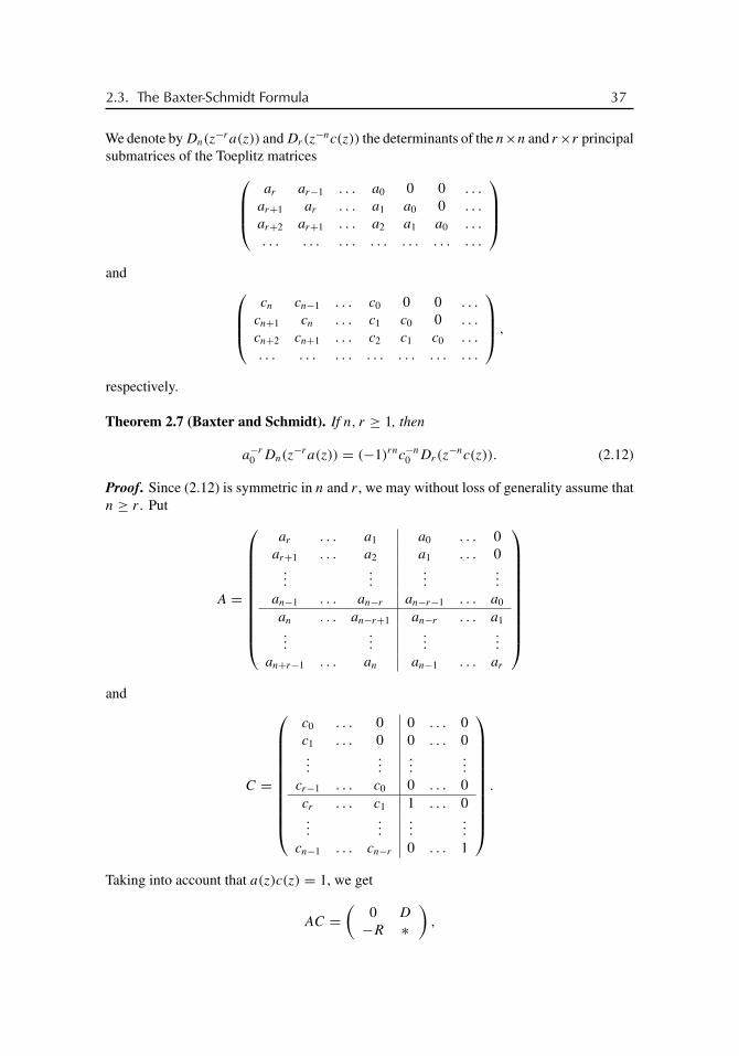
buch72005/10/5page 37

�

�

�

�

�

�

�

�

2.3. The Baxter-Schmidt Formula 37

We denote by Dn(z−ra(z)) and Dr(z

−nc(z)) the determinants of the n×n and r×r principalsubmatrices of the Toeplitz matrices⎛⎜⎜⎝

ar ar−1 . . . a0 0 0 . . .

ar+1 ar . . . a1 a0 0 . . .

ar+2 ar+1 . . . a2 a1 a0 . . .

. . . . . . . . . . . . . . . . . . . . .

⎞⎟⎟⎠and ⎛⎜⎜⎝

cn cn−1 . . . c0 0 0 . . .

cn+1 cn . . . c1 c0 0 . . .

cn+2 cn+1 . . . c2 c1 c0 . . .

. . . . . . . . . . . . . . . . . . . . .

⎞⎟⎟⎠ ,

respectively.

Theorem 2.7 (Baxter and Schmidt). If n, r ≥ 1, then

a−r0 Dn(z

−ra(z)) = (−1)rnc−n0 Dr(z

−nc(z)). (2.12)

Proof. Since (2.12) is symmetric in n and r , we may without loss of generality assume thatn ≥ r . Put

A =

⎛⎜⎜⎜⎜⎜⎜⎜⎜⎜⎜⎝

ar . . . a1 a0 . . . 0ar+1 . . . a2 a1 . . . 0

......

......

an−1 . . . an−r an−r−1 . . . a0

an . . . an−r+1 an−r . . . a1...

......

...

an+r−1 . . . an an−1 . . . ar

⎞⎟⎟⎟⎟⎟⎟⎟⎟⎟⎟⎠and

C =

⎛⎜⎜⎜⎜⎜⎜⎜⎜⎜⎜⎝

c0 . . . 0 0 . . . 0c1 . . . 0 0 . . . 0...

......

...

cr−1 . . . c0 0 . . . 0cr . . . c1 1 . . . 0...

......

...

cn−1 . . . cn−r 0 . . . 1

⎞⎟⎟⎟⎟⎟⎟⎟⎟⎟⎟⎠.

Taking into account that a(z)c(z) = 1, we get

AC =(

0 D

−R ∗)

,

buch72005/10/5page 38

�

�

�

�

�

�

�

�


where D is a lower-triangular (n − r) × (n − r) matrix whose diagonal elements are allequal to a0 and where R is the r × r matrix

R =⎛⎜⎝ a0cn . . . a0cn−r+1

......

ar−1cn + · · · + a0cn−r+1 . . . ar−1cn−r+1 + · · · + a0cn

⎞⎟⎠

=

⎛⎜⎜⎜⎝a0

a1 a0...

.... . .

ar−1 ar−2 . . . a0

⎞⎟⎟⎟⎠⎛⎜⎜⎜⎝

cn cn−1 . . . cn−r+1

cn+1 cn . . . cn−r+2...

.... . .

...

cn+r−1 cn+r−2 . . . cn

⎞⎟⎟⎟⎠ .

Clearly,

det A = Dn(z−ra(z)), det C = cr

0,

det AC = (−1)r(n−r)an−r0 (−1)r det R,

det R = ar0Dr(z

−nc(z)),

whence

cr0Dn(z

−ra(z)) = (−1)r(n−r)+ran0Dr(z

−nc(z)).

Since r(n − r) + r ≡ rn (mod 2), c0 = a−10 , a0 = c−1

0 , we therefore arrive at the desiredformula (2.12).

2.4 Widom’s FormulaLet now b be a Laurent polynomial,

b(t) =s∑

j=−r

bj tj (t ∈ T).

We are interested in a formula for the determinant Dn(b) of the Toeplitz band matrix Tn(b)

whose complexity is independent of n. If r ≤ 0 or s ≤ 0, then Tn(b) is triangular and henceDn(b) is the nth power of the entry on the main diagonal. Thus, assume r ≥ 1, s ≥ 1,b−r �= 0, and bs �= 0. We can write

b(t) = bst−r

r+s∏j=1

(t − zj ) (t ∈ T), (2.13)

where z1, . . . , zr+s are the zeros of the polynomial

zrb(z) = b−r + b−r+1z+ · · · + bszr+s . (2.14)

Theorem 2.8 (Widom). If the zeros z1, . . . , zr+s are pairwise distinct then, for every n ≥ 1,

Dn(b) =∑M

CMwnM, (2.15)

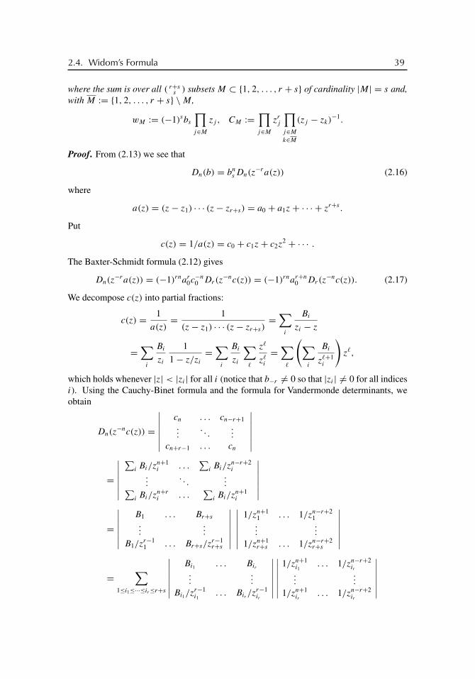
buch72005/10/5page 39

�

�

�

�

�

�

�

�

2.4. Widom’s Formula 39

where the sum is over all ( r+ss ) subsets M ⊂ {1, 2, . . . , r + s} of cardinality |M| = s and,

with M := {1, 2, . . . , r + s} \M ,

wM := (−1)sbs

∏j∈M

zj , CM :=∏j∈M

zrj

∏j∈M

k∈M

(zj − zk)−1.

Proof. From (2.13) we see that

Dn(b) = bns Dn(z

−ra(z)) (2.16)

where

a(z) = (z− z1) · · · (z− zr+s) = a0 + a1z+ · · · + zr+s .

Put

c(z) = 1/a(z) = c0 + c1z+ c2z2 + · · · .

The Baxter-Schmidt formula (2.12) gives

Dn(z−ra(z)) = (−1)rnar

0c−n0 Dr(z

−nc(z)) = (−1)rnar+n0 Dr(z

−nc(z)). (2.17)

We decompose c(z) into partial fractions:

c(z) = 1

a(z)= 1

(z− z1) · · · (z− zr+s)=

∑i

Bi

zi − z

=∑

i

Bi

zi

1

1− z/zi

=∑

i

Bi

zi

∑�

z�

z�i

=∑

�

(∑i

Bi

z�+1i

)z�,

which holds whenever |z| < |zi | for all i (notice that b−r �= 0 so that |zi | �= 0 for all indicesi). Using the Cauchy-Binet formula and the formula for Vandermonde determinants, weobtain

Dn(z−nc(z)) =

∣∣∣∣∣∣∣cn . . . cn−r+1...

. . ....

cn+r−1 . . . cn

∣∣∣∣∣∣∣=

∣∣∣∣∣∣∣∑

i Bi/zn+1i . . .

∑i Bi/z

n−r+2i

.... . .

...∑i Bi/z

n+ri . . .

∑i Bi/z

n+1i

∣∣∣∣∣∣∣=

∣∣∣∣∣∣∣B1 . . . Br+s

......

B1/zr−11 . . . Br+s/z

r−1r+s

∣∣∣∣∣∣∣∣∣∣∣∣∣∣

1/zn+11 . . . 1/zn−r+2

1...

...

1/zn+1r+s . . . 1/zn−r+2

r+s

∣∣∣∣∣∣∣=

∑1≤i1≤···≤ir≤r+s

∣∣∣∣∣∣∣Bi1 . . . Bir

......

Bi1/zr−1i1

. . . Bir /zr−1ir

∣∣∣∣∣∣∣∣∣∣∣∣∣∣

1/zn+1i1

. . . 1/zn−r+2ir

......

1/zn+1ir

. . . 1/zn−r+2ir

∣∣∣∣∣∣∣

buch72005/10/5page 40

�

�

�

�

�

�

�

�


=∑i∈M

Bi1 · · ·Bir

(zi1 · · · zir )n+1

∣∣∣∣∣∣∣1 . . . 1...

...

1/zr−1i1

. . . 1/zr−1ir

∣∣∣∣∣∣∣∣∣∣∣∣∣∣

1 . . . zr−1i1

......

1 . . . zr−1ir

∣∣∣∣∣∣∣=

∑i∈M

Bi1 · · ·Bir

(zi1 · · · zir )n+1

∏β>α

(1

ziβ

− 1

ziα

) ∏β>α

(ziβ − ziα )

=∑i∈M

Bi1 · · ·Bir

(zi1 · · · zir )n+1

∏β �=α

(ziβ − ziα )∏β

1

zr−1iβ

=∑M

⎛⎝∏i∈M

Bi

⎞⎠⎛⎝∏i∈M

z−n−1i

⎞⎠⎛⎜⎜⎝ ∏

i,k∈Mk �=i

(zi − zk)

⎞⎟⎟⎠ ∏i∈M

z−r−1i

=∑M

⎛⎝∏i∈M

Bi

⎞⎠⎛⎝∏i∈M

z−n−ri

⎞⎠⎛⎜⎜⎝ ∏

i,k∈Mk �=i

(zi − zk)

⎞⎟⎟⎠ . (2.18)

The coefficients Bi of the partial fraction decomposition are

Bi = −∏��=i

(zi − z�).

Hence

⎛⎝∏i∈M

Bi

⎞⎠⎛⎜⎜⎝ ∏

i,k∈Mk �=i

(zi − zk)

⎞⎟⎟⎠= (−1)r

∏i∈Mj∈M

(zi − zj )−1

∏i,�∈M��=i

(zi − z�)−1

∏i,k∈Mk �=i

(zi − zk)

= (−1)r+rs∏i∈Mj∈M

(zi − zj )−1. (2.19)

Combining (2.16), (2.17), (2.18), and (2.19), we arrive at the equality

Dn(b) = bns (−1)rnar+n

0

∑M

⎛⎝∏i∈M

z−n−ri

⎞⎠ (−1)r−rs

⎛⎜⎜⎝∏i∈Mj∈M

(zi − zj )−1

⎞⎟⎟⎠ .

buch72005/10/5page 41

�

�

�

�

�

�

�

�

2.5. Trench’s Formula 41

Since a0 = (−1)r+sz1 · · · zr+s , it follows that

Dn(b) = bns (−1)rn+(r+s)(r+n)+r+rs

∑M

⎛⎝∏j∈M

zn+ri

⎞⎠⎛⎜⎜⎝∏

i∈Mj∈M

(zi − zj )−1

⎞⎟⎟⎠ .

As rn+ (r + s)(r + n)+ r + rs ≡ 2rn+ 2rs + r(r + 1)+ sn ≡ sn (mod 2) and

∑M

⎛⎝∏j∈M

zn+ri

⎞⎠⎛⎜⎜⎝∏

i∈Mj∈M

(zi − zj )−1

⎞⎟⎟⎠ =∑M

⎛⎝∏j∈M

zn+ri

⎞⎠⎛⎜⎜⎝∏

k∈Mj∈M

(zi − zk)−1

⎞⎟⎟⎠ ,

we finally obtain (2.15).

Example 2.9. Let T (a) be the tridiagonal matrix considered in Section 2.2 and writea(t) = t−1(t − z1)(t − z2). Suppose z1 �= z2. There are exactly two sets M ⊂ {1, 2} ofcardinality |M| = 1, namely M = {1} and M = {2}. Thus, by Theorem 2.8,

w{1} = (−1)a1z1, C{1} = z1(z1 − z2)−1,

w{2} = (−1)a1z2, C{2} = z2(z2 − z1)−1,

Dn(a) = z1

z1 − z2(−1)nan

1zn1 +

z2

z2 − z1(−1)nan

1zn2 = (−1)nan

1zn+1

1 − zn+12

z2 − z1.

We leave it as an exercise to verify that this is in accordance with the formula provided byTheorem 2.6.

2.5 Trench’s FormulaLet b be as in Section 2.4. We now establish a formula for Dn(b) that is also applicable tothe case where the polynomial (2.14) has multiple zeros.

We denote by gn(z) the row

gn(z) = ( 1 z . . . zr−1 zr+n zr+n+1 . . . zr+n+s−1 ).

Let ξ1, . . . , ξm be the distinct roots of the polynomial (2.14) and let α1, . . . , αm be theirmultiplicities. We define Gn as the determinant of the (r + s)× (r + s) matrix Ar+s whosefirst α1 rows are gn(ξ1), g′n(ξ1), . . . , g(α1−1)

n (ξ1), whose next α2 rows are gn(ξ2), g′n(ξ2), . . . ,g(α2−1)

n (ξ2), and so on.

Theorem 2.10 (Trench). We have G0 �= 0 and

Dn(b) = (−1)nsbns

Gn

G0for every n ≥ 1. (2.20)

Confluent Vandermonde determinants. Before turning to the proof of this theorem, wecite the formula for the so-called confluent Vandermonde determinants. Let hβ(z) be the

buch72005/10/5page 42

�

�

�

�

�

�

�

�


row ( zβ zβ+1 . . . zβ+α−1 ). Given m distinct number ξ1, . . . , ξm and natural numbersα1, . . . , αm such that α1 + · · · + αm = α, we let

V (ξ1(β1, α1), . . . , ξm(βm, αm))

denote the determinant of the α × α matrix whose rows are

hβ1(ξ1), h′β1

(ξ1), . . . , h(α1−1)β1

(ξ1), . . . , hβm(ξm), h′βm

(ξm), . . . , h(αm−1)βm

(ξm).

In the case α1 = · · · = αm = 1, this is a pure Vandermonde determinant and hence

V (ξ1(β1, 1), . . . , ξα(βα, 1)) =∏

i

ξβi

i

∏j>i

(ξj − ξi).

Appropriate limit passages and l’Hospital’s rule therefore yield

V (ξ1(β1, α1), . . . , ξm(βm, αm)) =∏

i

ξαiβi

i

∏i

G(αi + 1)∏j>i

(ξj − ξi)αj αi , (2.21)

where G(α + 1) := (α − 1)!(α − 2)! . . . 1!0!.Proof of Theorem 2.10. By formula (2.21),

G0 = V (ξ1(0, α1), . . . , ξm(0, αm)) =∏

i

G(αi + 1)∏j>i

(ξj − ξi)αj αi �= 0.

Suppose first that the zeros z1, . . . , zr+s of the polynomial (2.14) are all simple. We showthat in this case the right-hand side of (2.20) coincides with the right-hand side of (2.15).Let M range over all subsets {j1, . . . , js} of {1, 2, . . . , r + s} whose cardinality is s and put{1, 2, . . . , r + s} \M =: {k1, . . . , kr}. Using Laplace’s expansion theorem, we obtain thatGn is

∑M

(−1)1+···+r+k1+···+kr

∣∣∣∣∣∣∣1 zk1 . . . zr−1

k1

......

...

1 zkr. . . zr−1

kr

∣∣∣∣∣∣∣∣∣∣∣∣∣∣

zr+nj1

. . . zr+n+s−1j1

......

zr+njs

. . . zr+n+s−1js

∣∣∣∣∣∣∣=

∑M

(−1)1+···+r+k1+···+kr (zj1 . . . zjs)r+n

∏α>β

(zkα− zkβ

)∏γ>δ

(zjγ− zjδ

). (2.22)

Permuting the rows 1, 2, . . . , r + s of G0 to k1, . . . , kr , j1, . . . , js shows that G0 equals

(−1)(k1−1)+(k2−2)+···+(kr−r)∏α>β

(zkα− zkβ

)∏γ>δ

(zjγ− zjδ

)∏γ,α

(zjγ− zkα

). (2.23)

buch72005/10/5page 43

�

�

�

�

�

�

�

�

2.6. Szegö’s Strong Limit Theorem 43

From (2.22) and (2.23) we get

Gn

G0=

∑M

(zj1 . . . zjs)r+n

∏γ,α

(zjγ− zkα

)−1

=∑M

⎛⎝∏j∈M

zj

⎞⎠n ∏j∈M

zrj

∏j∈M

k∈M

(zj − zk)−1

=∑M

((−1)sb−1s wM)nCM = (−1)snb−n

s

∑M

CMwnM,

which completes the proof in the case of simple zeros. If there are multiple zeros amongz1, . . . , zr+s , then the formula follows from what was just proved by the appropriate limitpassages.

2.6 Szegö’s Strong Limit TheoremLet b(t) =∑s

j=−r bj tj be a Laurent polynomial and suppose

b(t) �= 0 for t ∈ T and wind b = 0. (2.24)

In that case there is a function log b ∈ C(T) such that b = exp(log b). Clearly, log b isdetermined uniquely up to an additive constant in 2πiZ. Let (log b)k be the kth Fouriercoefficient of log b and put

G(b) = exp(log b)0, (2.25)

E(b) = exp∞∑

k=1

k(log b)k(log b)−k. (2.26)

Since b ∈ C∞(T), the function log b also belongs to C∞(T). This implies that (log b)k =O(1/|k|m) for every m ≥ 1 and shows that the series in (2.26) converges absolutely. Theconstants G(b) and E(b) are obviously independent of the particular choice of log b.

We know from Section 1.4 that if (2.24) holds, then

b(t) = bs

k∏i=1

(1− δi

t

)�i �∏j=1

(t − μj)σj ,

where δ1, . . . , δk, μ1, . . . , μ� are distinct, |δi | < 1, |μj | > 1, �1 + · · · + �k = r , andσ1 + · · · + σ� = s. On writing

log b(t) = log bs +k∑

i=1

�i log

(1− δi

t

)+

�∑j=1

σj log(−μj)+�∑

j=1

σj log

(1− t

μj

)

buch72005/10/5page 44

�

�

�

�

�

�

�

�


and using the formula log(1− z) = −z− z2/2− z3/3− · · · (|z| < 1), we get

(log b)0 = log bs +�∑

j=1

σj log(−μj),

(log b)n = −�∑

j=1

σj

nμnj

(n ≥ 1),

(log b)−n = −k∑

i=1

�iδni

n(n ≥ 1).

Thus, the constants (2.25) and (2.26) are

G(b) = bs(−1)s�∏

j=1

μσj

j , (2.27)

E(b) =k∏

i=1

�∏j=1

(1− δi

μj

)−�iσj

. (2.28)

Theorem 2.11 (Szegö’s strong limit theorem). If b is a Laurent polynomial satisfying(2.24), then

Dn(b) = G(b)nE(b)(1+O(qn)) as n→∞ (2.29)

with some constant q ∈ (0, 1).

Proof. Formula (2.20) and Laplace expansion of the determinant Gn show that

Dn(b) = (−1)nsbbs

G0V (δ1(0, �1), . . . , δk(0, �k))

× V (μ1(r + s, σ1), . . . , μ�(r + n, σ�)) (1+O(qn))

with

max | δi | / min |μj | < q < 1. (2.30)

By formula (2.21),

V (δ1(0, �1), . . . , δk(0, �k))

=∏

i

G(�i + 1)∏i2>i1

(δi2 − δi1)�i2 �i1 ,

V (μ1(r + s, σ1), . . . , μ�(r + n, σ�))

=∏j

μσi(r+n)j

∏j

G(σj + 1)∏

j2>j1

(μj2 − μj1)σj2 σj1 ,

buch72005/10/5page 45

�

�

�

�

�

�

�

�

2.7. The Szegö-Widom Theorem 45

G0 = V (δ1(0, �1), . . . , δk(0, �k), μ1(0, σ1), . . . , μ�(0, σ�))

=∏

i

G(�i + 1)∏j

G(σj + 1)

×∏i2>i1

(δi2 − δi1)�i2 �i1

∏j2>j1

(μj2 − μj1)σj2 σj1

∏j

∏i

(μj − δi)σj �i ,

whence

(−1)nsbbs

G0V (δ1(0, �1), . . . , δk(0, �k)) V (μ1(r + s, σ1), . . . , μ�(r + n, σ�))

= (−1)nsbns

⎛⎝∏j

μσj

j

⎞⎠n ∏j

μσj r

j

∏j

∏i

(μj − δi)−σj �i ,

and since∏j

μσj r

j

∏j

∏i

(μj − δi)−σj �i

=∏j

μσj r

j

∏j

(μ−σj r

j

∏i

(1− δi

μj

)−σj �i

)=

∏j

∏i

(1− δi

μj

)−σj �i

,

formulas (2.27) and (2.28) imply the assertion.

2.7 The Szegö-Widom TheoremThe road from Baxter-Schmidt through Widom and Trench led to a completely elementarybut rather computational proof of Szegö’s strong limit theorem. With a little bit of operatortheory, this theorem can be proved in a straightforward and very nifty way.

Trace class. Let (cjk)∞j,k=0 be an infinite matrix that defines a compact operator K on �2.

The operator K is said to be a Hilbert-Schmidt operator if

∞∑j,k=0

|cjk|2 <∞,

and K is called a trace class operator if it is the product of two Hilbert-Schmidt operators.The Hilbert-Schmidt and trace class operators form two-sided ideals in the algebra of allbounded operators.

Operator determinants. Let K be a trace class operator and let {λj (K)}Nj=1 (N finiteor N = ∞) be the sequence of its eigenvalues, each eigenvalue repeated according to itsalgebraic multiplicity. Then

N∑j=1

|λj (K)| <∞,

buch72005/10/5page 46

�

�

�

�

�

�

�

�


and the determinant det(I +K) is defined by

det(I +K) =N∏

j=1

(1+ λj (K)).

The operator I +K is invertible if and only if det(I +K) �= 0. If K and L are trace classoperators, then

det(I +K)(I + L) = det(I +K) det(I + L). (2.31)

If C is an invertible operator, then

det(I + CKC−1) = det C(I +K)C−1 = det(I +K). (2.32)

For n ≥ 1, let Pn : �2 → �2 be the projection defined by

Pn : {x0, x1, x2, . . . } �→ {x0, x1, . . . , xn−1, 0, . . . }.We identify Pn(I +K)Pn with the n×n matrix (δjk+ cjk)

n−1j,k=1, where δjk is the Kronecker

delta. Then, if K is of trace class,

limn→∞ det Pn(I +K)Pn = det(I +K). (2.33)

Prologue. Recall that H(a) is the Hankel operator given by the infinite matrix (aj+k+1)∞j,k=0.

Obviously,

H(a) is Hilbert-Schmidt ⇐⇒∞∑

n=1

n|an|2 <∞. (2.34)

Now let b be a Laurent polynomial satisfying (2.24). We then can write b = b−b+ with

b−(t) =r∏

i=1

(1− δi

t

), b+(t) = bs

s∏j=1

(t − μj), (2.35)

where |δi | < 1 and |μj | > 1. The matrix T (b−1− ) is upper triangular with 1 on the main

diagonal, while T (b−1+ ) is lower triangular with (bs

∏(−μj))

−1 on the main diagonal. Thisimplies that

PnT (b−1− )Pn = T (b−1

− )Pn, PnT (b−1+ )Pn = PnT (b−1

+ ) (2.36)

and

det Tn(b−1− ) = 1, det Tn(b

−1+ ) =

⎛⎝bs

s∏j=1

(−μj)

⎞⎠−n

= G(b)−n (2.37)

(recall (2.27)). By Proposition 1.3,

T (b)T (b−1) = I −H(b)H (b−1) (2.38)

buch72005/10/5page 47

�

�

�

�

�

�

�

�

2.7. The Szegö-Widom Theorem 47

and

T (b−1+ )T (b)T (b−1

− ) = T (b−)T (b−1− )−H(b−1

+ )H (b)T (b−1− )

= I −H(b−1+ )H (b)T (b−1

− ).

We therefore deduce from (2.34) that both T (b)T (b−1) and T (b−1+ )T (b)T (b−1

− ) are of theform I + trace class operator.

Theorem 2.12 (Szegö-Widom limit theorem). If b is a Laurent polynomial without zeroson the unit circle and with winding number zero, then

limn→∞

Dn(b)

G(b)n= det T (b)T (b−1).

Proof. From (2.36) and (2.37) we see that

det PnT (b−1+ )T (b)T (b−1

− )Pn = det PnT (b−1+ )PnT (b)PnT (b−1

− )Pn

= det Tn(b−1+ )Tn(b)Tn(b

−1− ) = Dn(b)/G(b)n. (2.39)

On the other hand, since T (b−1+ )T (b)T (b−1

− )− I is of trace class, we infer from (2.33) that

limn→∞ det PnT (b−1

+ )T (b)T (b−1− )Pn = det T (b−1

+ )T (b)T (b−1− ),

and (2.32) shows that

det T (b−1+ )T (b)T (b−1

− ) = det T (b)T (b−1− )T (b−1

+ ) = det T (b)T (b−1).

To compute the operator determinant det T (b)T (b−1) we need two auxiliary results.We abbreviate det T (b)T (b−1) to E(b).

Lemma 2.13. Let f±, g±, h± be Laurent polynomials in W± without zeros on T and withwinding number zero. Then

E(f−g+h+) = E(f−g+)E(f−h+), E(g−h−f+) = E(g−f+)E(h−f+). (2.40)

Proof. Using (2.31) and (2.32), we obtain

E(f−g+h+) = det T (f−g+h+)T (f −1− h−1

+ g−1+ )

= det T (f−)T (g+)T (h+)T (f −1− )T (h−1

+ )T (g−1+ )

= det T (g−1+ )T (f−)T (g+)T (h+)T (f −1

− )T (h−1+ )

= det T (g−1+ )T (f−)T (g+)T (f −1

− ) det T (f−)T (h+)T (f −1− )T (h−1

+ )

= det T (f−)T (g+)T (f −1− )T (g−1

+ ) det T (f−)T (h+)T (f −1− )T (h−1

+ )

= E(f−g+)E(f−h+).

The proof of the second equality of (2.40) is analogous.

buch72005/10/5page 48

�

�

�

�

�

�

�

�


Lemma 2.13 implies that

E(b) =r∏

i=1

s∏j=1

E

[(1− δi

t

)(t − μj)

], (2.41)

and hence we are left with computing the factors on the right-hand side of (2.41).

Lemma 2.14. If |δ| < 1 and |μ| > 1, then

E

[(1− δ

t

)(t − μ)

]=

(1− δ

μ

)−1

. (2.42)

Proof. Put c(t) = (1− δ/t)/(t − μ). By virtue of Proposition 1.3,

E(c) = det T (c)T (c−1) = det(I −H(c)H (c−1)).

Clearly, I −H(c)H (c−1) equals

I −

⎛⎜⎜⎝1 0 0 . . .

0 0 . . .

0 . . .

. . .

⎞⎟⎟⎠⎛⎜⎜⎝

(c−1)−1 (c−1)−2 (c−1)−3 . . .

(c−1)−2 (c−1)−3 . . .

(c−1)−3 . . .

. . .

⎞⎟⎟⎠

=

⎛⎜⎜⎝1− (c−1)−1 ∗ ∗ . . .

0 1 ∗ . . .

0 0 1 . . .

. . . . . . . . . . . .

⎞⎟⎟⎠ ,

which shows that E(c) = 1− (c−1)−1. The −1st Fourier coefficient of c−1 is

(c−1)−1 =[(

1+ δ

t+ δ2

t2+ · · ·

)(− 1

μ

)(1+ t

μ+ t2

μ2+ · · ·

)]0

= − 1

μ

(δ + δ2

μ+ δ3

μ2+ · · ·

)= − δ

μ

1

1− δ/μ,

whence 1− (c−1)−1 = 1/(1− δ/μ.

Combining (2.41) and (2.42) we arrive at the formula

det T (b)T (b−1) =r∏

i=1

s∏j=1

(1− δi

μj

)−1

,

which is in accordance with (2.28).

2.8 Geronimo, Case, Borodin, OkounkovJacobi’s theorem says that if A is an invertible m×m matrix, then the determinant of theupper-left n×n block of A−1 is equal to the determinant of the lower-right (m−n)×(m−n)

block of A divided by det A. Let Qn : �2 → �2 be the projection acting by the rule

Qn : {x0, x1, x2, . . . } �→ {0, . . . , 0, xn, xn+1, . . . }.

buch72005/10/5page 49

�

�

�

�

�

�

�

�

2.8. Geronimo, Case, Borodin, Okounkov 49

Thus, Qn = I − Pn. If A = I +K with a trace class operator K , then

det PnA−1Pn = det QnAQn

det A. (2.43)

Indeed, with A replaced by PmAPm, this is Jacobi’s theorem, and for general A the formulafollows from (2.33) after the limit passage m→∞.

Now let b = b−b+, where b− and b+ are given by (2.35). Put

u = b−b−1+ , v = b−1

− b+.

Since uv = 1, we have T (u)T (v) = I −H(u)H (v). Notice that H(u)H (v) is in the traceclass.

The remarkable formula contained in the following theorem was established by Geron-imo and Case [127] in 1979 (for positive symbols b) and rediscovered by Borodin andOkounkov [31] in 2000.

Theorem 2.15. Let b be a Laurent polynomial without zeros on the unit circle and withwinding number zero. Then for all n ≥ 1,

Dn(b)

G(b)n= det QnT (u)T (v)Qn

det T (u)T (v)= det(I −QnH(u)H (v)Qn)

det(I −H(u)H (v)). (2.44)

Proof. By (2.39) and (2.43),

Dn(b)

G(b)n= det PnT (b−1

+ )T (b)T (b−1− )Pn = det QnT (b−)T −1(b)T (b+)Qn

det T (b−)T −1(b)T (b+),

and as

T (b−)T (b)T (b+) = T (b−)T (b−1+ )T (b−1

− )T (b+) = T (u)T (v) = I −H(u)H (v),

we arrive at the assertion.

Since det(I −QnH(u)H (v)Qn)→ 1 as n→∞, formula (2.44) implies at once theSzegö-Widom limit theorem:

limn→∞

Dn(b)

G(b)n= 1

det T (u)T (v)= det T −1(v)T −1(u)

= det T (b−1+ )T (b−)T (b+)T (b−1

− )

= det T (b−)T (b+)T (b−1− )T (b−1

+ ) = det T (b)T (b−1).

buch72005/10/5page 50

�

�

�

�

�

�

�

�


Exercises

1. Prove that

det

⎛⎜⎜⎜⎝d1 x . . . x

x d2 . . . x...

.... . .

...

x x . . . dn

⎞⎟⎟⎟⎠= x(d1 − x) · · · (dn − x)

(1

x+ 1

d1 − x+ · · · + 1

dn − x

).

2. Prove that

det

⎛⎜⎜⎜⎜⎜⎝x a1 a2 . . . an

a1 x a2 . . . an

a1 a2 x . . . an

......

.... . .

...

a1 a2 a3 . . . x

⎞⎟⎟⎟⎟⎟⎠= (x + a1 + a2 + · · · + an)(x − a1)(x − a2) · · · (x − an).

3. Let b(t) = x + t + t−1. Prove that

Dn(b) = xn −(

n− 11

)xn−2 +

(n− 2

2

)xn−4 −+ · · · .

4. Let ωn = e2πi/n. Prove that

det

⎛⎜⎜⎜⎜⎜⎝1 1 1 . . . 11 ωn ω2

n . . . ωn−1n

1 ω2n ω4

n . . . ω2(n−1)n

......

......

1 ωn−1n ω2(n−1)

n . . . ω(n−1)(n−1)n

⎞⎟⎟⎟⎟⎟⎠ = nn/2 i−(n−1)(n+2)/2.

5. Prove that

det

⎛⎜⎜⎜⎜⎝1 1

213 . . . 1

n12

13

14 . . . 1

n+1...

......

...1n

1n+1

1n+2 . . . 1

2n−1

⎞⎟⎟⎟⎟⎠ = [1! 2! · · · (n− 1)!]3n! (n+ 1)! · · · (2n− 1)!

and that, with G(m) := (m− 2)! · · · 2! 1! 0!, this is the same as

(G(n+ 1))4

G(2n+ 1).

buch72005/10/5page 51

�

�

�

�

�

�

�

�

Exercises 51

6. Let a1 = 1, a2 = 3, a3 = 240, a4 = 1512000. Which of the three numbers

1512030752000, 1536288768000, 1541291254000

is a5?

7. Let b(t) = 8t2 − 54t + 101 − 54t−1 + 8t−2. Prove that Dn(b) > 26n−1 for allsufficiently large n.

8. Let b ∈ P satisfy (2.24) and let b = b−b+ be a Wiener-Hopf factorization.

(a) Show that

T (b)T (b−1) = eT (log b−)eT (log b+)e−T (log b−)e−T (log b−).

(b) Show that

tr (T (log b−)T (log b+)− T (log b+)T (log b−))

= tr H(log b)H((log b) ) =∞∑

k=1

k(log b)k(log b)−k.

9. Let b ∈ P and suppose T (b) is invertible. Show that det PnT−1(b)Pn = 1/G(b)n

and that, therefore, the Szegö-Widom limit theorem can also be written as

det PnT (b)Pn det PnT−1(b)Pn → det T (b)T (b−1).

10. Let b ∈ Pr and suppose that b has no zeros on T and winding number zero. Provethat

Dn(b−1) = G(b−1)n det T (b−1)T (b)

for all n ≥ r .

11. Let |αi | < 1 and |βj | < 1. Prove that

Dn

(1∏

(1− αj t)∏

(1− βj t−1)

)=

∏i,j

1

1− αiβj

for all n ≥ 1.

12. Let a ∈ W and suppose that a(t) > 0 for t ∈ T. Prove that if there are nonzeroconstants G(a) and E(a) such that

Dn(a) = G(a)nE(a) for all n ≥ r,

then a−1 ∈ Pr .

13. (a) Show that if H(a) is a trace class operator, then |a1| + |a2| + |a3| + · · · <∞.

(b) Show that if |a1| + 2 |a2| + 3 |a3| + · · · <∞, then H(a) is of trace class.

(c) Prove that if a ∈ C2(T), then H(a) is a trace class operator.

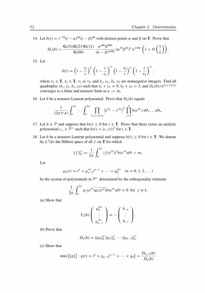
buch72005/10/5page 52

�

�

�

�

�

�

�

�


14. Let b(t) = t−70(t − α)40(t − β)60 with distinct points α and β on T. Prove that

Dn(b) = G(31)G(21)G(11)

G(60)

α400β600

(α − β)1000(α10β20)n n1100

(1+O

(1

n

)).

15. Let

b(t) =(

1− τ1

t

)δ1(

1− t

τ1

)γ1 (1− τ2

t

)δ2(

1− t

τ2

)γ2

,

where τ1 ∈ T, τ2 ∈ T, τ1 �= τ2, and δ1, γ1, δ2, γ2 are nonnegative integers. Find allquadruples (δ1, γ1, δ2, γ2) such that δ1 + γ1 = 9, δ2 + γ2 = 3, and Dn(b)/nδ1γ1+δ2γ2

converges to a finite and nonzero limit as n→∞.

16. Let b be a nonzero Laurent polynomial. Prove that Dn(b) equals

1

(2π)n n!∫ 2π

0· · ·

∫ 2π

0

∏1≤j<k≤n

∣∣eiθj − eiθk∣∣2

n∏j=1

b(eiθj ) dθ1 . . . dθn.

17. Let b ∈ P and suppose that b(t) ≥ 0 for t ∈ T. Prove that there exists an analyticpolynomial c+ ∈ P+ such that b(t) = |c+(t)|2 for t ∈ T.

18. Let b be a nonzero Laurent polynomial and suppose b(t) ≥ 0 for t ∈ T. We denoteby L2(b) the Hilbert space of all f on T for which

‖f ‖2b :=

1

2π

∫ 2π

0|f (eiθ )|2b(eiθ )dθ <∞.

Let

ϕn(t) = tn + ϕ(n)n−1t

n−1 + · · · + ϕ(n)0 (n = 0, 1, 2, . . . )

be the system of polynomials in P+ determined by the orthogonality relations

1

2π

∫ 2π

0ϕj (e

iθ )ϕk(eiθ )b(eiθ )dθ = 0 for j �= k.

(a) Show that

Tn(b)

⎛⎜⎝ ϕ(n)0...

ϕ(n)n−1

⎞⎟⎠ = −⎛⎜⎝ b−n

...

b−1

⎞⎟⎠ .

(b) Prove that

Dn(b) = ‖ϕ0‖2b ‖ϕ1‖2

b · · · ‖ϕn−1‖2b.

(c) Show that

min{‖g‖2

b : g(t) = tn + gn−1tn−1 + · · · + g0

} = Dn+1(b)

Dn(b)

buch72005/10/5page 53

�

�

�

�

�

�

�

�

Notes 53

and that the minimum is attained at g = ϕn.

(d) Deduce that

‖ϕn‖2b → G(b) := exp

(1

2π

∫ 2π

0log b(eiθ )dθ

).

(e) Let χn(eiθ ) := einθ . Deduce that the set

closL2(b)

∞⋃n=0

lin {χ0, χ1, . . . , χn}

does not coincide with L2(b).

Notes

The material of Sections 2.1 and 2.2 is well known. From [161] we learned that Theorem2.4 goes back to D. E. Rutherford [239], [240]. In [117], [118], the result is referred toas Bloch’s theorem. For real-valued symbols, Theorem 2.4 is essentially also in [145] and[176], and paper [243] shows that an arbitrary tridiagonal Toeplitz matrix is similar to aHermitian tridiagonal Toeplitz matrix (see formula (11.1)).

The Baxter-Schmidt formula (Theorem 2.7) was established in [19]. The proof givenhere is based on a proof by Tismenetsky [266] and a remark of a referee of [266]. Theorem2.8 is a result of Widom [290] in the reformulation of [243]. Our proof is from [67]. Theorem2.10 was proved by Trench [278] for n ≥ r + s + 1 and subsequently by Berg [24] for alln ≥ 1. For more on Sections 2.3 to 2.5, the reader may also consult paper [32].

In 1915, Szegö [262] proved what is now called his “first limit theorem”: If b ∈ L1,b ≥ 0, and log b ∈ L1, then Dn(b)/Dn−1(b)→ G(b) as n→∞. At the turn of the 1950s,he was told by S. Kakutani that it would be desirable to have a second-order asymptoticformula for Dn(b), because this would prove a formula by Lars Onsager for the spontaneousmagnetization of the two-dimensional Ising model (we learned of this story from [13]). As aconsequence of this, Szegö published his “strong limit theorem” in 1952 [263]: If b > 0 andthe derivative b′ satisfies a Hölder condition, then Dn(b)/G(b)n → E(b) as n→∞. Baxter[18], Hirschman [164], and Devinatz [102] then became to understand that the positivityof b may be replaced by the “index zero condition” (2.24), and they gave different proofsof the formula Dn(b) = G(b)nE(b)(1 + o(1)) for symbols b from classes much largerthan the class of Laurent polynomials. The development culminated with Widom’s paper[294]. Basor [13] writes: “The proofs of the various Szegö theorems were for the most partdifficult, indirect, and worst of all gave no ‘natural’indication why the terms in the expansion,especially the E(b), occurred. Fortunately, this state of affairs was considerably altered in1976 by Widom [294], whose elegant application of ideas from operator theory extendedSzegö’s theorem to the block case and gave easy proofs of the results.” For more detailson Szegö’s limit theorem we refer the reader to the books [70] and [71]. Comprehensivestudies of trace class operators and infinite determinants are in [133], [217], [254].

The story with formula (2.44) started in 1979, but let us begin 20 years later. InJune 1999, during an MSRI workshop on random matrices, Alexander Its and Percy Deift

buch72005/10/5page 54

�

�

�

�

�

�

�

�


raised the question of whether there is a general formula that expresses the determinantof the Toeplitz matrix Tn(a) as the Fredholm determinant of an operator I − K , where K

acts on �2{n, n + 1, . . . }. Borodin and Okounkov [31] then showed that such a formulaindeed exists. The form in which we cited their formula in Theorem 2.15 is due to HaroldWidom. The original proof by Borodin and Okounkov is based on representation theoryand combinatorics, in particular on results by Okounkov on infinite wedge and randompartitions and a theorem by I. M. Gessel expressing a Toeplitz determinant as a sum overpartitions of products of Schur functions. Two other proofs were subsequently given byBasor and Widom [16]. The first of these proofs uses an identity for det Tn−1(a) / det Tn(a)

containing just H(b)H(c), which was established by Widom in 1973, and the second is afurther development of the argument employed by Basor and J. W. Helton in 1980 to provethe Szegö-Widom limit theorem. The two proofs by Basor and Widom are operator-theoreticand very lucid. A third operator-theoretic proof was found [37]. It follows from the identity

T −1n (a) = Tn(a

−1+ )(I − PnT (c)QnXQnT (b)Pn)Tn(a

−1− ),

where X = (I − QnH(b)H(c)Qn)−1. This identity, which lifts formula (2.44) from the

determinant level to the matrix level, was obtained in 1980 by B. Silbermann and one of theauthors [63]. The proof given here is from [38]. It is a modification of the second proof of[16] and is the probably shortest proof of identity (2.44).

In July 2003, the people involved in formula (2.44) and its proof since 1999 receivedan email from Percy Deift. This email was as follows. “Recently Jeff Geronimo showedme a 1979 paper of his with Ken Case in which they wrote down the Borodin-Okounkovformula in the context of proving strong Szegö. The reference is [127]. See, in particular,formula VII.28 on page 308. It’s quite remarkable that the formula was already known in1979. The proof of the formula by Geronimo-Case is inverse-scattering theoretic and is theanalogue of Dyson’s second-derivative log det formula for the Schrödinger case.” There isnothing we can add, except for our congratulations to Jeff Geronimo and Ken Case on theirbrilliant feat, for our gratification of the eventual recognition of their great success, and forexpressing our regret that their names are missing in [16], [31], [37], [38].

Simon’s book [255] contains a proof of (2.44) under the most general (and natural)smoothness conditions on b: It is only required that

∑∞k=−∞ |k| |bk|2 < ∞. This proof is

based on the proof given here and on additional technical arguments due to Rowan Killipand Percy Deift.

Exercises 1 to 5 are from [113] and [208]. The observation of Exercise 10 wasprobably already known to Szegö (see [145]). Exercise 11 is due to Baxter [17] (see also[79] and [174]). Solutions to Exercises 10 and 12 are in [63] and [67]. The problem ofcharacterizing the symbols a for which H(a) is of trace class had been open for a long timebefore it was completely solved by Peller [202], [203] (see also his recent capital monograph[204]). Simple solutions to Exercise 13 can be found in [67]. For Exercise 15 see [64]. Theformula of Exercise 16 goes back to Szegö [262]. The result of Exercise 17 is due to Fejérand F. Riesz; see, e.g., [145]. Exercise 18 summarizes classical results by Szegö and werefer the reader to [108], [145], [255] for proofs and more material.

The link between Exercises 8(a) and 8(b) is the formula

det eAeBe−Ae−B = etr (AB−BA), (2.45)

buch72005/10/5page 55

�

�

�

�

�

�

�

�

Notes 55

which is true whenever A and B are bounded on �2 and AB − BA is a trace class operatoron �2. Formula (2.45) appeared first in [158] and [206]. It was used by Widom in [294] toshow that

det T (b)T (b−1) = exp∞∑

k=1

k(log b)k(log b)−k

and thus to recover Szegö’s original strong limit theorem from Theorem 2.12. The proofsof (2.45) given in [158] and [206] are difficult. Recently Torsten Ehrhardt [106] found aremarkably simple proof of the stronger identity

det eAeBe−A−B = etr 12 (AB−BA). (2.46)

This identity is true for arbitrary A, B ∈ B(�2) for which AB − BA is of trace class. Notethat (2.46) implies that

det eA+Be−Ae−B = etr 12 (AB−BA), (2.47)

and that multiplication of (2.46) and (2.47) yields (2.45).

Further results: Fisher-Hartwig symbols. The formulas established by Widom andTrench can be employed to compute the determinants Dn(b) for an arbitrary Laurent polyno-mial b. However, in order to understand the asymptotic behavior of Dn(b), additional workmust be done (see, for example, Exercise 14). In the following we cite some asymptoticresults for Laurent polynomials in the so-called Fisher-Hartwig class.

Let first

b(t) =(

1− τ

t

)δ (1− t

τ

)γ

c(t), t ∈ T,

where τ ∈ T, δ and γ are nonnegative integers, and c is a Laurent polynomial without zeroson T and with wind c = 0. In the case where c is identically 1 (and thus absent), an exactformula for Dn(b) was established in [68]:

Dn

[(1− τ

t

)δ (1− t

τ

)γ]

= G(1+ δ)G(1+ γ )

G(1+ γ + δ)

G(n+ 1)G(n+ 1+ γ + δ)

G(n+ 1+ δ)G(n+ 1+ γ ), (2.48)

where G(1) = 1 and G(m) = (m − 2)! · · · 2! 1! 0! for m ≥ 2. (Two elementary proofs ofthis identity can be found in [73].) The right-hand side of (2.48) is

G(1+ δ)G(1+ γ )

G(1+ γ + δ)nδγ (1+ o(1)) as n→∞.

Now suppose that c is present. We put

G(c) = exp(log c)0, E(c) = exp∞∑

k=1

k(log c)k(log c)−k,

c+(t) = exp∞∑

k=1

(log c)ktk, c−(t) = exp

∞∑k=1

(log c)−kt−k.

buch72005/10/5page 56

�

�

�

�

�

�

�

�


Clearly, c = G(c)c−c+. In [69], it is shown that

Dn

[(1− τ

t

)δ (1− t

τ

)γ

c(t)

]/Dn

[(1− τ

t

)δ(1− t

τ

)γ]

= G(c)nE(c)

c−(τ )γ c+(τ )δ

(1+O

(1

n

)).

Things are essentially more complicated for symbols with more than one zero on the unitcircle. Let now

b(t) =N∏

j=1

(1− τj

t

)δj(

1− t

τj

)γj

c(t), t ∈ T,

where τ1, . . . , τN are distinct points on T, δj and γj are nonnegative integers, and c is asabove. The asymptotics of Dn(b) in this case was obtained in [64]. The result is as follows.Without loss of generality assume that

γ := γ1 + · · · + γN ≤ δ1 + · · · + δN =: δ(otherwise pass to the adjoint matrix). Put zj = γj + δj ,

M = {(m1, . . . , mN) : mj ∈ Z, 0 ≤ mj ≤ zj , m1 + · · · +mn = γ },

Q = max

⎧⎨⎩N∑

j=1

(mjzj −m2j ) : (m1, . . . , mN) ∈M

⎫⎬⎭ ,

M∗ =⎧⎨⎩(m1, . . . , mN) ∈M :

N∑j=1

(mjzj −m2j ) = Q

⎫⎬⎭ .

Then

Dn(b) = G(c)nE(c) nQ (1+O(1/n))

×⎡⎣ ∑

(m1,...,mn)∈M∗Am1,...,mN

(τ

m11 · · · τmN

N

τγ11 · · · τ γN

N

)n

+O

(1

n

)⎤⎦ , (2.49)

where G(c) and E(c) are as above and

Am1,...,mN=

∏i �=j

(1− τi

τj

)(mi−zi )mj

×N∏

j=1

G(zj −mj + 1)G(mj + 1)

G(zj + 1)

N∏j=1

1

c−(τj )mj c+(τj )

zj−mj. (2.50)

The constellation where δj = γj for all j is especially interesting. In this case the asymp-totics of Dn(b) was described earlier by Widom [293]. Thus, let

b(t) =N∏

j=1

|t − τj |2γj c(t), t ∈ T.

buch72005/10/5page 57

�

�

�

�

�

�

�

�

Notes 57

If (m1, . . . , mN) ∈M, then

N∑j=1

(mj · 2γj −m2j ) ≤

N∑j=1

(m2j + γ 2

j −m2j ) =

N∑j=1

γ 2j =

N∑j=1

(γj · 2γj − γ 2j )

and equality holds if and only if mj = γj for all j . Hence Q = γ 21 + · · · + γ 2

N andM∗ = {(γ1, . . . , γN)}. Formulas (2.49) and (2.50) therefore yield

Dn(b) = G(c)nE(c) nγ 21 +···+γ 2

N A

(τ

γ11 · · · τ γN

N

τγ11 · · · τ γN

N

)n

(1+O(1/n))

= G(c)nE(c) A nγ 21 +···+γ 2

N (1+O(1/n)) (2.51)

with

A =∏i �=j

(1− τi

τj

)−γiγj N∏j=1

G(2γi − γi + 1)G(γi + 1)

G(2γi + 1)

N∏j=1

1

c−(τj )γj c+(τj )

γj.

Since

∏i �=j

(1− τi

τj

)−γiγj

=∏i>j

[(1− τi

τj

)−γiγj(

1− τj

τi

)−γj γi

]

=∏i>j

∣∣∣∣1− τi

τj

∣∣∣∣−2γiγj

=∏i>j

|τi − τj |−2γiγj =∏i �=j

|τi − τj |−γiγj ,

we obtain

A = G(c)γ∏i �=j

|τi − τj |−γiγj

N∏j=1

1

c(τj )γj

N∏j=1

G(γj + 1)2

G(2γj + 1). (2.52)

As already said, (2.51) and (2.52) are already in [293].

buch72005/10/5page 58

�

�

�

�

�

�

�

�

buch72005/10/5page 59

�

�

�

�

�

�

�

�

Chapter 3

Stability

For a ∈ W and n ∈ {1, 2, 3, . . . }, the n × n Toeplitz matrix Tn(a) is defined by (2.1). Wenow consider the sequence {Tn(a)}∞n=1 as an entity associated with T (a). In this chapter,we study the following problem: Is there an n0 ≥ 1 and an M ∈ (0,∞) such that Tn(a) isinvertible for all n ≥ n0 and

‖T −1n (a)‖p ≤ M for all n ≥ n0 ? (3.1)

This problem plays a key role in the theory of large Toeplitz matrices. Since

‖T −1n (a)‖2 = 1

σmin(Tn(a))≥ rad T −1

n (a),

where σmin(Tn(a)) is the smallest singular value of Tn(a) and rad T −1n (a) stands for the spec-

tral radius of T −1n (a), question (3.1) for p = 2 is equivalent to asking whether σmin(Tn(a))

stays away from zero, and if the answer is yes, we can conclude that the eigenvalues ofTn(a) are bounded away from zero as n→∞.

3.1 Strong and Weak ConvergenceThroughout this section, X and Y are Banach spaces. We denote by B(X, Y ) the Banachspace of all bounded linear operators from X to Y , and we let K(X, Y ) stand for the Banachspace of all compact operators from X to Y . As usual, we put B(X,X) =: B(X) andK(X, X) =: K(X).

Let {An}∞n=1 be a sequence of operators An ∈ B(X, Y ). We say that An converges toan operator A ∈ B(X, Y )

uniformly if ‖An − A‖ → 0,strongly if ‖Anx − Ax‖ → 0 for all x ∈ X,weakly if |(Anx, y)− (Ax, y)| → 0 for all x ∈ X and all y ∈ Y ∗;

here Y ∗ is the dual space of Y , and for z ∈ Y and y ∈ Y ∗, we let (z, y) denote the value ofthe functional y at z.

59

buch72005/10/5page 60

�

�

�

�

�

�

�

�

60 Chapter 3. Stability

Theorem 3.1 (Banach and Steinhaus). Let {An}∞n=1 be a sequence of operators An ∈B(X, Y ) such that {Anx}∞n=1 is a convergent sequence in Y for each x ∈ X. Thensupn≥1 ‖An‖ < ∞, the operator A defined by Ax := limn→∞Anx belongs to B(X, Y ),and ‖A‖ ≤ lim infn→∞ ‖An‖.

This theorem, which is also known as the uniform boundedness principle, is provedin every text on functional analysis.

Proposition 3.2. If K ∈ K(X, Y ) and the operators An ∈ B(Y ) converge strongly toA ∈ B(Y ), then the operators AnK converge uniformly to AK .

Proof. Let B1 := {x ∈ X : ‖x‖ ≤ 1} and S1 := {x ∈ X : ‖x‖ = 1}. Fix ε > 0.Since K maps B1 to a set whose closure is a compact subset of Y , there exists some finitecollection of elements x1, . . . , xN ∈ B1 such that for each x ∈ S1 we can find an xj satisfying‖Kx −Kxj‖ < ε. Clearly,

‖AnKx − AKx‖ ≤ ‖An‖ ‖Kx −Kxj‖ + ‖AnKxj − AKxj‖ + ‖A‖ ‖Kxj −Kx‖≤ ‖An‖ ε + ‖AnKxj − AKxj‖ + ‖A‖ ε.

Theorem 3.1 implies that ‖An‖ ≤ M <∞ for all n, and as An converges strongly to A, thenorms ‖AnKxj −AKxj‖ are less than ε for all j provided n is sufficiently large. Thus, forn large enough,

‖AnKx − AKx‖ ≤ (M + 1+ ‖A‖) ε = (M + 1+ ‖A‖)ε‖x‖,

which shows that ‖AnK − AK‖ → 0.

Proposition 3.3. If K ∈ K(X, Y ) and the operators An ∈ B(X) converge weakly toA ∈ B(X), then the operators KAn converge strongly to KA.

Proof. Fix an arbitrary x ∈ X. Since (Anx, y) → (Ax, y) for all x ∈ X and all y ∈ Y ∗,we see that the operators Tn defined by Tn : Y ∗ → C, y �→ (Anx, y) converge strongly tothe operator T : y �→ (Ax, y). Thus, by Theorem 3.1, supn≥1 ‖Anx‖ = supn≥1 ‖Tn‖ <∞.This shows that the sequence {Anx}∞n=1 is bounded. Contrary to what we want, let us assumethat KAnx does not converge to KAx. Then there exist an ε > 0 and a sequence {nk} suchthat

‖KAnkx −KAx‖ ≥ ε for all k. (3.2)

Since K is compact and {Ank}∞k=1 is bounded, there exists a subsequence {nkj

} of {nk} suchthat {KAnkj

x} has a limit z in Y . The weak convergence of KAnkjto KA implies that

z = KAx, whence ‖KAnkjx −KAx‖ → 0 as j →∞. But this contradicts (3.2).

Let �p (1 ≤ p ≤ ∞) be the spaces introduced in Section 1.2. We denote by ‖ · ‖p

both the norm in �p and B(�p). Furthermore, we let c0 denote the closed subspace of �∞that is constituted by the sequences that converge to zero. The norm in c0 is the ‖ ·‖∞ norm.

buch72005/10/5page 61

�

�

�

�

�

�

�

�

3.2. Stable Sequences 61

For n = 1, 2, . . . , let Pn and Qn be the projections on �p and c0 defined by

Pn : {x0, x1, x2, . . . } �→ {x0, x1, . . . , xn−1, 0, 0, . . . }, (3.3)

Qn : {x0, x1, x2, . . . } �→ {0, . . . , 0︸︷︷︸n

, xn, xn+1, . . . }. (3.4)

Note that Pn +Qn = I . It is clear that the operators Pn do not converge uniformly. Theoperators Pn converge strongly to I on �p if 1 ≤ p <∞ and on c0, but they do not convergestrongly on �∞.

3.2 Stable SequencesThroughout this section we assume that the underlying Banach space X is c0 or �p (1 ≤p ≤ ∞).

For n = 1, 2, . . . , we denote by Xn the space Cn with the �p norm if X = �p andwith the �∞ norm if X = c0. On identifying

{x0, x1, . . . , xn−1} and {x0, x1, . . . , xn−1, 0, 0, . . . },we can identify Xn with the image of X under the projection Pn given by (3.3). If A is ann× n matrix, we think of A as an operator on (the column space) Xn and therefore ‖A‖ iswell defined. Notice that ‖A‖ = ‖PnAPn‖, where ‖A‖ is the norm of A as an element ofB(Xn) and ‖PnAPn‖ stands for the norm of the (well-defined) operator PnAPn ∈ B(X).

Let {An} := {An}∞n=1 be a sequence of n× n matrices An. The sequence {An} is saidto be stable on X if

lim supn→∞

‖A−1n ‖ <∞,

where, by convention, ‖A−1n ‖ := ∞ if An is not invertible. Equivalently, {An} is stable on

X if and only if there exist n0 ≥ 1 and M ∈ (0,∞) such that An is invertible for all n ≥ n0

and ‖A−1n ‖ ≤ M for all n ≥ n0.

Lemma 3.4. Suppose X = c0 or X = �p with 1 < p <∞. Let {An} be a sequence of n×n

matrices An and assume there is an operator A ∈ B(X) such that An → A and A∗n → A∗strongly. If

lim infn→∞ ‖A−1

n ‖ <∞ (3.5)

then A is invertible.

Proof. If (3.5) holds, there are n1 < n2 < · · · and M ∈ (0,∞) such that ‖A−1nk‖ ≤ M . For

every x ∈ X, ‖Pnkx‖ = ‖A−1

nkAnk

Pnkx‖ ≤ M‖Ank

Pnkx‖. Since Pnk

→ I and Ank→ A

strongly, it follows that ‖x‖ ≤ M‖Ax‖. Hence, A is injective and has a closed range.The dual space (�p)∗ may be identified with �q (1/p + 1/q = 1) and the dual space

(c0)∗ with �1. Since ‖(A∗n)−1‖ = ‖A−1

n ‖, we can repeat the argument of the precedingparagraph to obtain that ‖x‖ ≤ M‖A∗x‖ for all x ∈ X∗. This shows that A∗ is injective.

buch72005/10/5page 62

�

�

�

�

�

�

�

�


Hence, A has dense range. Together with what was already proved, this implies that theoperator A is invertible.

Proposition 3.5. Suppose X is c0 or �p with 1 ≤ p < ∞. Let {An} be a sequence ofn × n matrices An and assume that An → A strongly on X for some invertible operatorA ∈ B(X). Then the following are equivalent:

(i) {An} is stable;(ii) An is invertible for all sufficiently large n and A−1

n → A−1 strongly on X.

Proof. To show (ii)⇒ (i), note that if A−1n → A−1 strongly, then lim sup ‖A−1

n ‖ is finite byvirtue of Theorem 3.1. So let us prove the implication (i)⇒ (ii). For every y ∈ X,

‖A−1n Pny − A−1y‖ ≤ ‖A−1

n Pny − PnA−1y‖ + ‖PnA

−1y − A−1y‖. (3.6)

The second term on the right of (3.6) goes to zero, because Pn → I strongly. The first termon the right of (3.6) is

‖A−1n (Pny − AnPnA

−1y)‖ ≤ M‖Pny − AnPnA−1y‖ = o(1),

since AnPnA−1 → AA−1 = I strongly.

3.3 The Baxter-Gohberg-Feldman TheoremIn this section we show that if a ∈ W , then the sequence {Tn(a)} is stable if and only ifT (a) is invertible.

Toeplitz operators on c0. In the previous section, we have seen that in connection withstability problems the passage to adjoint operators is useful. The dual space of �1 may beidentified with �∞, and as soon as the space �∞ enters the scene, difficulties arise, becausethe projections Pn do not converge strongly on �∞. To tackle questions located in the space�1, it is often advantageous to think of �1 as the dual space of c0.

Let us denote by ‖ · ‖0 both the norm in c0 and B(c0). It is easily seen that the infiniteToeplitz matrix T (a) induces a bounded operator on c0 if and only if a ∈ W , in which case‖T (a)‖0 = ‖a‖W . As in the proofs of Propositions 1.1 and 1.2 one can show that if a ∈ W ,then the Hankel operator H(a) is compact on c0. Finally, the reasoning of the proof ofTheorem 1.9 gives that if a ∈ W , then T (a) is Fredholm on c0 if and only if a has no zeroson T, in which case Ind T (a) = −wind a and T (a) is invertible if wind a = 0.

Lemma 3.6. Suppose X is a linear space, P and Q are complementary projections on X

(that is, P 2 = P , Q2 = Q, P +Q = I ), and A is an invertible linear operator on X. Thenthe compression PAP | Im P of A to the range Im P of P is invertible if and only if thecompression QA−1Q | Im Q of A−1 to the range Im Q of Q is invertible. In that case

(PAP )−1P = PA−1P − PA−1Q(QA−1Q)−1QA−1P.

buch72005/10/5page 63

�

�

�

�

�

�

�

�

3.3. The Baxter-Gohberg-Feldman Theorem 63

Proof. We have

PAP(PA−1P − PA−1Q(QA−1Q)−1QA−1P)

= PA(I −Q)A−1P − PA(I −Q)A−1Q(QA−1Q)−1QA−1P

= P − PAQA−1P − 0+ PAQA−1P = P ,

and similarly, (PA−1P − PA−1Q(QA−1Q)−1QA−1P)PAP = P .

Theorem 3.7 (Baxter, Gohberg, and Feldman). Let X be one of the spaces c0 or �p

(1 ≤ p ≤ ∞) and let a ∈ W . Then

lim supn→∞

‖T −1n (a)‖ <∞ if T (a) is invertible, (3.7)

limn→∞‖T

−1n (a)‖ = ∞ if T (a) is not invertible. (3.8)

Thus, {Tn(a)}∞n=1 is stable if and only if a has no zeros on T and wind a = 0.

Proof. Suppose first that X = c0 or X = �p with 1 < p <∞.Assertion (3.8) is immediate from Lemma 3.4. So assume T (a) is invertible. By

Proposition 1.3, T (a)T (a−1) = I −H(a)H (a−1), whence

T −1(a) = T (a−1)+ T −1(a)H(a)H (a−1) =: T (a−1)+K.

The operator K is compact due to Proposition 1.2. Recall that Qn := I−Pn. Since Qn → 0strongly, we deduce from Proposition 3.2 that

‖QnKQn | Im Qn‖ = ‖QnKQn‖ ≤ ‖QnK‖ = o(1),

which implies that

QnT−1(a)Qn | Im Qn = QnT (a−1)Qn | Im Qn +Kn

with ‖Kn‖ → 0. The operator QnT (a−1)Qn | Im Qn has the same matrix as T (a−1), and asT (a−1) is invertible together with T (a) (Theorem 1.9), it follows that QnT

−1(a)Qn | Im Qn

is invertible for all sufficiently large n and that for every ε > 0 there is an n0(ε) such that

‖(QnT−1(a)Qn)

−1Qn‖ < (1+ ε)‖T −1(a−1)‖for all n ≥ n0(ε). For these n we obtain from Lemma 3.6 that the matrices Tn(a) =PnT (a)Pn | Im Pn are invertible and that

(PnT (a)Pn)−1Pn = PnT

−1(a)Pn − PnT−1(a)Qn(QnT

−1(a)Qn)−1QnT

−1(a)Pn.

This implies that

‖T −1n (a)‖ ≤ ‖T −1(a)‖ + (1+ ε)‖T −1(a)‖ ‖T −1(a−1)‖ ‖T −1(a)‖

and hence gives (3.7).

buch72005/10/5page 64

�

�

�

�

�

�

�

�


Let now X be the space �1. From what was already proved, we know thatlim sup ‖T −1

n (a)‖0 < ∞ if T (a) is invertible on c0 and that lim ‖T −1n (a)‖0 = ∞ if T (a)

is not invertible on c0. As ‖T −1n (a)‖0 = ‖T −1

n (a)‖1 and as T (a) is invertible on c0 if andonly if T (a) is invertible on �1, we arrive at (3.7) and (3.8) for X = �1. Finally, the pre-ceding argument can be employed to reduce the case X = �∞ to the (by now settled) caseX = �1.

Corollary 3.8. Let X be c0 or �p with 1 ≤ p < ∞ and a ∈ W . If T (a) is invertible, thenthe operators T −1

n (a)Pn converge strongly to T −1(a) on X.

Proof. The proof is immediate from Proposition 3.5 and Theorem 3.7.

Corollary 3.8 tells us that if T (a) is invertible, we can approximately solve the infinitesystem T (a)x = y by replacing it with the finite system Tn(a)x(n) = Pny, x(n) ∈ Im Pn.This is called the finite section method. In this connection it is of interest to know somethingabout the first n0 such that Tn(a) is invertible for all n ≥ n0. In the case of banded matrices,the following result reveals that this n0 is in general not an astronomic number.

Proposition 3.9. Let b be a Laurent polynomial and suppose b has no zeros on the unit circleT and wind b = 0. Choose a number α satisfying (1.23). Then there is a constant C(b, α),depending only on b and α, such that Tn(b) is invertible whenever C(b, α) e−2αn < 1.

Proof. By Lemma 3.6, Tn(b) = PnT (b)Pn | Im Pn is invertible if and only if the operatorAn := QnT

−1(b)Qn | Im Qn is invertible. We have

T −1(b) = T (b−1+ )T (b−1

− ) = T (b−1)−K, K := H(b−1+ )H (b−1

− ).

Since the operator QnT (b−1)Qn | Im Qn has the same matrix as T (b−1), the operator An iscertainly invertible if ‖QnKQn‖ ‖T −1(b−1)‖ < 1. But from Lemma 1.17 we infer that

‖QnKQn‖ ≤ ‖QnH(b−1+ )‖ ‖H(b−1

− )Qn‖

≤⎛⎝ ∞∑

j=0

(j + 1)∣∣(b−1

+ )n+j

∣∣⎞⎠⎛⎝ ∞∑j=0

(j + 1)∣∣(b−1

− )−n−j

∣∣⎞⎠ = O(e−2αn).

3.4 Silbermann TheoryIn this section we present Silbermann’s approach to the stability problem. This approachyields another proof to Theorem 3.7 and, moreover, allows us to extend this theorem toToeplitz matrices with certain perturbations.

We begin with the analogue of Proposition 1.3 for finite Toeplitz matrices. For n =1, 2, 3, . . . , we define the operators Wn on �p by

Wn : {x0, x1, x2, . . . } �→ {xn−1, . . . , x1, x0, 0, 0, . . . }. (3.9)

Obviously, W 2n = Pn. It is also easy to verify that

WnTn(a)Wn = Tn(a), (3.10)

buch72005/10/5page 65

�

�

�

�

�

�

�

�

3.4. Silbermann Theory 65

where, as usual, a(t) := a(1/t) (t ∈ T).

Proposition 3.10 (Widom). If a, b ∈ W then

Tn(ab) = Tn(a)Tn(b)+ PnH(a)H (b)Pn +WnH(a)H(b)Wn.

Proof. From Proposition 1.3 we obtain

Tn(ab) = PnT (ab)Pn = PnT (a)T (b)Pn + PnH(a)H (b)Pn,

and since

PnT (a)T (b)Pn = PnT (a)PnT (b)Pn + PnT (a)QnT (b)Pn

= Tn(a)Tn(b)+ PnT (a)QnT (b)Pn,

it suffices to check that

PnT (a)QnT (b)Pn = WnH(a)H(b)Wn. (3.11)

But it is easily seen that the j, k entry (1 ≤ j, k ≤ n) of each side of (3.11) is

a−n+j−1bn−k+1 + a−n+j−2bn−k+2 + · · · .

We now suppose that X is c0 or �p with 1 < p < ∞. Let F denote the set of allsequences {An} := {An}∞n=1 of n× n matrices An such that supn≥1 ‖An‖ < ∞. It is easilyseen that F is a Banach algebra with the algebraic operations

{An} + {Bn} := {An + Bn}, α{An} := {αAn}, {An}{Bn} := {AnBn}and the norm ‖{An}‖ := supn≥1 ‖An‖. We define S as the subset of F that is constituted bythe sequences {An} for which there exist two operators A ∈ B(X) and A ∈ B(X) such that

An → A, A∗n → A∗, WnAnWn → A, WnA∗nWn → A∗

strongly. It is not difficult to check that S is a closed subalgebra of F, and hence S itself isa Banach algebra. Finally, let J be the set of all sequences {An} ∈ F that are of the form

An = PnKPn +WnLWn + Cn (3.12)

with compact operators K and L and with ‖Cn‖ → 0 as n→∞.

Lemma 3.11 (Silbermann). J is a closed two-sided ideal of S.

Proof. Let An be of the form (3.12). Since Wn → 0 weakly, we deduce from Proposition3.3 that An → K strongly. Similarly, A∗n → K∗, WnAnWn → L, WnA

∗nWn → L∗ strongly.

Thus, J is a subset of S. It is clear that J is a linear space.To prove that J is closed, notice first that, by Theorem 3.1,

‖K‖ ≤ lim infn→∞ ‖An‖, ‖L‖ ≤ lim inf

n→∞ ‖WnAnWn‖.

buch72005/10/5page 66

�

�

�

�

�

�

�

�


Consequently, if {A(j)n }∞j=1 is a Cauchy sequence in J, then the sequences {K(j)}∞j=1 and

{L(j)}∞j=1 are Cauchy sequences in K(X). This implies that there exist operators K andL in K(X) such that K(j) → K and L(j) → L uniformly. Now it follows easily that‖{A(j)

n } − {An}‖ → 0 as j →∞ for some {An} ∈ S. This proves that J is closed.Finally, let {Bn} ∈ S and {An} ∈ J. Then

BnAn = BnPnKPn + BnWnLWn + BnCn

= PnBnKPn +Wn(WnBnWn)PnLWn + BnCn

= PnBKPn +WnBLWn + C ′n

with ‖C ′n‖ → 0, since Bn → BK and WnBnWnPnL → BL uniformly due to Proposition3.2. Consideration of adjoints shows that {AnBn} is also in J.

Theorem 3.12 (Silbermann). Let X be c0 or �p with 1 < p <∞. A sequence {An} ∈ S isstable if and only if A and A are invertible in B(X) and the coset {An} + J is invertible inthe quotient algebra S/J. Moroever, if {Rn} + J is the inverse of {An} + J in S/J, then

Bn := Rn + Pn(A−1 − R)Pn +Wn(A

−1 − R)Wn

satisfies AnBn = Pn + C ′n and BnAn = Pn + C ′′n with ‖C ′n‖ → 0 and ‖C ′′n‖ → 0.

Proof. Suppose the sequence {An} is stable. Then A is invertible by Lemma 3.4. Since‖(WnAnWn)

−1‖ = ‖A−1n ‖, the sequence {WnAnWn} is also stable, and hence, again by

Lemma 3.4, A is invertible. The stability of {An} implies the existence of a sequence{Bn} ∈ F such that BnAn = Pn + Cn with ‖Cn‖ → 0 (simply take Bn = A−1

n for allsufficiently large n). Using Proposition 3.5, it is not difficult to see that {Bn} belongs to S.Thus, {Bn} + J is a left inverse of {An} + J. Analogously one can show the {An} + J isinvertible from the right.

Conversely, suppose now that A and A are invertible and that {Rn} + J is the inverseof {An} + J. Then

AnRn = Pn + PnKPn +WnLWn + Cn,

where K and L are compact and ‖Cn‖ → 0. Passage to the strong limit n → ∞ givesAR = I+K and AR = I+L. Thus, S := A−1−R = −A−1K and T := A−1−R = −AL

are also compact. Put

Bn = Rn + PnSPn +WnT Wn.

Then {Bn} ∈ S and, by Proposition 3.2,

AnBn = Pn + PnKPn +WnLWn + Cn + AnPnSPn + AnWnT Wn

= Pn + Pn(K + AnPnS)Pn +Wn(L+WnAnWnT )Wn + Cn

= Pn + Pn(K + AS)Pn +Wn(L+ AT )Wn + C ′n= Pn + C ′n

buch72005/10/5page 67

�

�

�

�

�

�

�

�

3.4. Silbermann Theory 67

with ‖C ′n‖ → 0. Consideration of adjoints yields that BnAn = Pn + C ′′n with‖C ′′n‖ → 0.

An infinite matrix is said to have finite support if at most finitely many of its entries arenonzero. Clearly, infinite matrices with finite support generate compact operators. Recallthat a is defined by a(t) := a(1/t) (t ∈ T).

Theorem 3.13 (Silbermann). Let X be c0 or �p with 1 ≤ p ≤ ∞ and let

An = Tn(a)+ PnKPn +WnLWn,

where a ∈ W and K and L are matrices with finite support. Put

A = T (a)+K, A = T (a)+ L.

Then

lim supn→∞

‖A−1n ‖ <∞ if A and A are invertible, (3.13)

limn→∞‖A

−1n ‖ = ∞ if A or A is not invertible. (3.14)

Consequently, {An}∞n=1 is stable if and only if both A and A are invertible.

Proof. We first consider the case where X = c0 or X = �p with 1 < p <∞.If lim inf ‖A−1

n ‖ <∞, A is invertible by virtue of Lemma 3.4. Since ‖(WnAnWn)−1‖

= ‖A−1n ‖, we can apply Lemma 3.4 to the sequence {WnAnWn} to obtain that A is invertible

whenever lim inf ‖A−1n ‖ <∞. This completes the proof of (3.14).

Let now A and A be invertible. It is clear that {An} ∈ S. Thus, (3.13) will followfrom Theorem 3.12 once we have shown that {An} + J is invertible in S/J. As {An} + J ={Tn(a)} + J, we are left to prove that {Tn(a)} + J is invertible. But if A = T (a) + K isinvertible, then T (a) is Fredholm and a ∈ GW . By Proposition 3.10,

Tn(a−1)Tn(a) = Pn − PnH(a−1)H (a)Pn −WnH(a−1)H(a)Wn,

and since all occurring Hankel operators are compact, it follows that

{PnH(a−1)H (a)Pn +WnH(a−1)H(a)Wn} ∈ J.

Thus, {Tn(a−1)}+J is a left inverse of {Tn(a)}+J. Similarly one can show that {Tn(a

−1)}+Jis a right inverse of {Tn(a)} + J. This proves that {Tn(a)} + J is invertible, as desired.

To dispose of the case where X = �1, we proceed as in the proof of Theorem 3.7.Define Bn := Tn(a) + PnK

∗Pn + WnL∗Wn, where K∗ and L∗ are the usual Hermitian

adjoints of the matrices K and L. By what was already proved, lim sup ‖B−1n ‖0 < ∞ if

B = T (a)+K∗ and B = T (a)+L∗ are invertible on c0, while lim inf ‖B−1n ‖0 = ∞ if B or

B is not invertible on c0. But ‖B−1n ‖0 = ‖(B−1

n )∗‖1 = ‖A−1n ‖1, and B and B are invertible

on c0 if and only if B∗ = A and B∗ = A are invertible on �1. This gives (3.13) and (3.14)for X = �1. The �∞ case can be reduced to the �1 case by the same reasoning.

Corollary 3.14. Let X be c0 or �p with 1 ≤ p <∞ and let An = Tn(a)+PnKPn+WnLWn

where a ∈ W and K and L are finitely supported. Then the operators A−1n Pn converge

strongly to (T (a)+K)−1 on X if and only if both T (a)+K and T (a)+ L are invertible.

buch72005/10/5page 68

�

�

�

�

�

�

�

�


Proof. This follows from Proposition 3.5 and Theorem 3.13.

3.5 Asymptotic InversesThe sequence {Bn} delivered by Theorem 3.12 is an asymptotic inverse for An: we haveA−1

n = Bn + Cn with ‖Cn‖ → 0 (notice that if ‖Pn − AnBn‖ → 0 and {An} is stable,then ‖A−1

n − Bn‖ ≤ ‖A−1n ‖ ‖Pn − AnBn‖ → 0). In the special case An = Tn(a) we have

A = T (a) and A = T (a), and when proving Theorem 3.13, we saw that Rn = Tn(a−1)

does the desired job, whence R = T (a−1) and R = T (a−1). Thus, on defining

K(a) := T −1(a)− T (a−1), K(a) := T −1(a)− T (a−1), (3.15)

for a ∈ GW with wind a = 0, we obtain

T −1n (a) = Tn(a

−1)+ PnK(a)Pn +WnK(a)Wn + Cn (3.16)

with ‖Cn‖ → 0 on c0 and �p for 1 ≤ p < ∞ (note that the proof of the convergence‖C ′n‖ → 0 in Theorem 3.12 also works for �1).

Here are some alternative expressions for the operators (3.15). From Proposi-tion 1.3 we infer that T (a)T (a−1) = I − H(a)H (a−1), whence T −1(a) − T (a−1) =T −1(a)H(a)H (a−1). This shows that

K(a) = T −1(a)H(a)H (a−1), K(a) = T −1(a)H (a)H(a−1). (3.17)

Combining (3.17) and Proposition 1.2 we see that K(a) and K(a) are compact. Anal-ogously, starting with T (a−1)T (a) = I − H(a−1)H (a), we get T −1(a) − T (a−1) =H(a−1)H (a)T −1(a) and thus

K(a) = H(a−1)H (a)T −1(a), K(a) = H(a−1)H(a)T −1(a). (3.18)

Given a Wiener-Hopf factorization a = a−a+, we can also write

K(a) = T (a−1+ )T (a−1

− )− T (a−1+ a−1

− ) = −H(a−1+ )H (a−1

− ), (3.19)

K(a) = T (a−1− )T (a−1

+ )− T (a−1− a−1

+ ) = −H(a−1− )H(a−1

+ ). (3.20)

Finally, from (3.19) and Exercise 2 of Chapter 1 we obtain

K(a) = −H(a−1+ )H (a−1

− ) = −H(a−1a−)H (a+a−1)

= −H(a−1)T (a−)T (a+)H (a−1) = −H(a−1)T −1(a)H (a−1) (3.21)

and analogously,

K(a) = −H(a−1)T −1(a)H(a−1). (3.22)

In the case of Toeplitz band matrices, we can show that the norm of the matrices Cn

in (3.16) decays exponentially.

Theorem 3.15. Let b be a Laurent polynomial without zeros on T and with winding numberzero. Choose an α satisfying (1.23) and let 1 ≤ p ≤ ∞. Then (3.16) holds with a replacedby b and with ‖Cn‖p = O(e−αn).

buch72005/10/5page 69

�

�

�

�

�

�

�

�

3.5. Asymptotic Inverses 69

Proof. From Proposition 3.10 and formula (3.10) we see that T −1n (b) equals

Tn(b−1)+ T −1

n (b)PnH(b)H (b−1)Pn +WnT−1n (b)PnH (b)H(b−1)Wn. (3.23)

We have

T −1n (b)PnH(b)H (b−1)Pn = T −1

n (b)Pn(I − T (b)T (b−1))Pn

= T −1n (b)Pn(T (b)T −1(b)− T (b)T (b−1))Pn = T −1

n (b)PnT (b)K(b)Pn

= T −1n (b)PnT (b)PnK(b)Pn + T −1

n (b)PnT (b)QnK(b)Pn

= PnK(b)Pn + T −1n (b)PnT (b)QnK(b)Pn. (3.24)

Let b = b−b+ be the Wiener-Hopf factorization (1.19). By virtue of (3.19), K(b) =−H(b−1

+ )H (b−1− ). Using Lemma 3.6 we obtain as in the proof of Proposition 3.9 that

‖QnK(b)‖p ≤ M1

∞∑j=0

(j + 1)∣∣(b−1

+ )n+j

∣∣ ≤ M1

∞∑j=0

M2e−α(n+j) = O(e−αn).

Since T −1n (b) = O(1) due to Theorem 3.7, we arrive at the conclusion that (3.24), that is,

the second term of (3.23), is PnK(b)Pn + O(e−αn). Analogously, one can show that thethird term of (3.23) is WnK(b)Wn +O(e−αn).

Corollary 3.16. Let b be a Laurent polynomial without zeros on T and suppose the windingnumber is zero. Let α satisfy (1.23) and let 1 ≤ p ≤ ∞. Then for each natural number k,

‖T −1n (b)Pk − T −1(b)Pk‖p = O(e−αn) as n→∞.

Proof. For j ≥ 0, let ej ∈ �p be the sequence defined by (ej )k = 1 for k = j and (ej )k = 0for k �= j . Clearly, it suffices to prove that

‖T −1n (b)ej − T −1(b)ej‖p = O(e−αn)

for each fixed j . Let n ≥ j . By (3.16),

T −1n (b)ej − T −1(b)ej

= Tn(b−1)ej + Pn(T

−1(b)− T (b−1))Pnej − T −1(b)ej +WnK(b)Wnej + Cnej

= −QnT−1(b)ej +WnK(b)Wnej + Cnej . (3.25)

Let b(t) = ∑rj=−r bj t

j . Then H(b) = H(b)Pr . Since Wnej = en−j , we therefore

obtain from (3.18) that ‖WnK(b)Wnej‖p ≤ ‖H(b−1)H(b)‖p ‖PrT−1(b)en−r‖p. As

‖PrT−1(b)en−r‖p is the �p norm of the first r components of the (n − r)th column of

the matrix T −1(b), we deduce from Lemma 1.17 and Proposition 1.18 that the norm‖PrT

−1(b)en−r‖p is O(e−αn). Also by Lemma 1.17 and Proposition 1.18, ‖QnT−1(b)‖p =

O(e−αn). Finally, because ‖Cnej‖p = O(e−αn) by virtue of Theorem 3.15, all three termsin (3.25) have norm O(e−αn).

Corollary 3.17. Under the hypotheses of Corollary 3.16,

‖PkT−1n (b)Pn − PkT

−1(b)‖p = O(e−αn) as n→∞.

buch72005/10/5page 70

�

�

�

�

�

�

�

�


0 20 40 60 80 100

0

0.2

0.4

0.6

0.8

1

1.2

Figure 3.1. The componentwise error |xj − x(99)j | against j = 0, . . . , 98.

Proof. Put En = T −1n (b)Pk−T −1(b)Pk . Corollary 3.16 says that if we consider En on c0 or

�p (1 ≤ p ≤ ∞), then ‖En‖ = O(e−αn). This implies that ‖E∗n‖ = O(e−αn) for the adjoint

operator E∗n = PkT

−1n (b)Pn − PkT

−1(b). As �1 = c∗0 and �p = (�q)∗ with 1/p + 1/q = 1for 1 < p ≤ ∞, we arrive at the assertion.

Example 3.18. The symbol b(t) = −2− 3it − 2t2 − 3t3 + t−1 − 2it−2 + 3t−3 generatesan invertible Toeplitz operator T (b). (To see this, plot b(T).) Choose x ∈ �2 by xj = 1for 0 ≤ j ≤ 99 and xj = 0 for j ≥ 100 and put y = T (b)x. Obviously, only thefirst 103 components of y are nonzero. The equation T99(b)x(99) = P99y has a uniquesolution, and Figure 3.1 shows the componentwise error |xj − x

(99)j | versus j = 0, . . . , 98.

It is clearly seen that P50x(99) is a good approximation to P50x, but that x(99) and P99x

differ heavily in their last components. For example, the last two components of x(99) are0.5082− 0.7108i and 2.0239− 0.0622i (while those of P99x are 1 and 1). Things changedramatically when passing from 99 to 100: we have x(100) = P100x exactly and MATLABreports ‖x(100) − P100x‖∞ < 2 · 10−15. Figure 3.2 shows the norms ‖x(n) − Pnx‖∞ and‖x(n) − Pnx‖2 versus n.

Example 3.19. Let b(t) = 5+t−t2+t3−t−2. The operator T (b) is invertible and hence wecan solve the equation T (b)x = y for each y ∈ �2 approximately by passing to the truncatedsystems Tn(b)x(n) = Pny. We choose 200 vectors xj of length 100 randomly from the unitsphere S99 of the Euclidean space R100 with the uniform distribution, extend xj by zeros toa sequence in �2, and put yj = T (b)xj . Then we solve the 200 systems Tn(b)x

(n)j = Pnyj

for n = 30, n = 60, and n = 90. The logarithmic error log10 ‖Pnxj − x(n)j ‖2 of the

computational results mildly fluctuates around −2 for n = 30, n = 60, n = 90, that is,there is no significant improvement when increasing n. However, the improvement in a

buch72005/10/5page 71

�

�

�

�

�

�

�

�

3.5. Asymptotic Inverses 71

0 20 40 60 80 100−1

0

1

2

3

4

5

6

7

8

9

Figure 3.2. The norms ‖x(n) − Pnx‖∞ (solid) and ‖x(n) − Pnx‖2 (dashed) versusn for 5 ≤ n ≤ 105.

0 50 100 150 200−20

−18

−16

−14

−12

−10

−8

−6

−4

−2

0

Figure 3.3. Let T (b)xj = yj with 200 random vectors xj of length 100. The pictureshows log10 ‖P30xj−P30x

(n)j ‖2 versus j = 1, . . . , 200 for the 200 systemsTn(b)x

(n)j = Pnyj

with n = 30 (upper curve), n = 60 (middle curve), and n = 90 (lower curve).

fixed set of components is drastic. Figure 3.3 shows that log10 ‖P30xj −P30x(n)j ‖2 fluctuates

around the values −2, −12, and −16 for n = 30, n = 60, and n = 90, respectively.

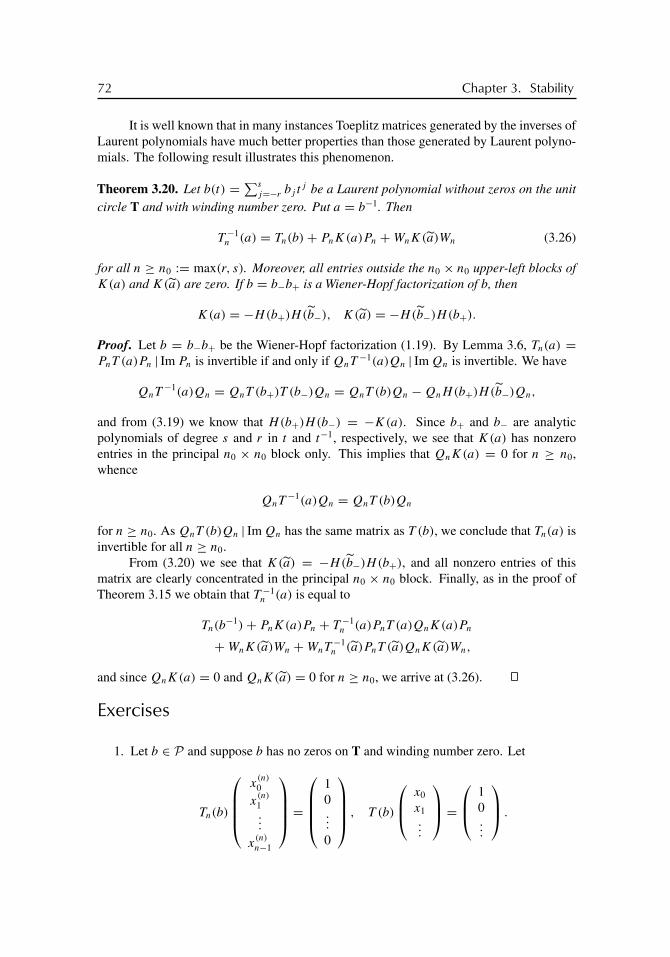
buch72005/10/5page 72

�

�

�

�

�

�

�

�


It is well known that in many instances Toeplitz matrices generated by the inverses ofLaurent polynomials have much better properties than those generated by Laurent polyno-mials. The following result illustrates this phenomenon.

Theorem 3.20. Let b(t) = ∑sj=−r bj t

j be a Laurent polynomial without zeros on the unitcircle T and with winding number zero. Put a = b−1. Then

T −1n (a) = Tn(b)+ PnK(a)Pn +WnK(a)Wn (3.26)

for all n ≥ n0 := max(r, s). Moreover, all entries outside the n0 × n0 upper-left blocks ofK(a) and K(a) are zero. If b = b−b+ is a Wiener-Hopf factorization of b, then

K(a) = −H(b+)H (b−), K(a) = −H(b−)H(b+).

Proof. Let b = b−b+ be the Wiener-Hopf factorization (1.19). By Lemma 3.6, Tn(a) =PnT (a)Pn | Im Pn is invertible if and only if QnT

−1(a)Qn | Im Qn is invertible. We have

QnT−1(a)Qn = QnT (b+)T (b−)Qn = QnT (b)Qn −QnH(b+)H (b−)Qn,

and from (3.19) we know that H(b+)H(b−) = −K(a). Since b+ and b− are analyticpolynomials of degree s and r in t and t−1, respectively, we see that K(a) has nonzeroentries in the principal n0 × n0 block only. This implies that QnK(a) = 0 for n ≥ n0,whence

QnT−1(a)Qn = QnT (b)Qn

for n ≥ n0. As QnT (b)Qn | Im Qn has the same matrix as T (b), we conclude that Tn(a) isinvertible for all n ≥ n0.

From (3.20) we see that K(a) = −H(b−)H(b+), and all nonzero entries of thismatrix are clearly concentrated in the principal n0 × n0 block. Finally, as in the proof ofTheorem 3.15 we obtain that T −1

n (a) is equal to

Tn(b−1)+ PnK(a)Pn + T −1

n (a)PnT (a)QnK(a)Pn

+WnK(a)Wn +WnT−1n (a)PnT (a)QnK(a)Wn,

and since QnK(a) = 0 and QnK(a) = 0 for n ≥ n0, we arrive at (3.26).

Exercises

1. Let b ∈ P and suppose b has no zeros on T and winding number zero. Let

Tn(b)

⎛⎜⎜⎜⎝x

(n)0

x(n)1...

x(n)n−1

⎞⎟⎟⎟⎠ =

⎛⎜⎜⎜⎝10...

0

⎞⎟⎟⎟⎠ , T (b)

⎛⎜⎝ x0

x1...

⎞⎟⎠ =⎛⎜⎝ 1

0...

⎞⎟⎠ .

buch72005/10/5page 73

�

�

�

�

�

�

�

�

Exercises 73

Show that

x(n)0 = Dn−1(b)

Dn(b), x0 = 1

G(b),

deduce that Dn(b)/Dn−1(b) converges to G(b) exponentially fast, and use this insightto conclude that Dn(b)/G(b)n converges to a finite and nonzero limit.

2. Show that Corollary 3.8 is not true for p = ∞.

3. Let a ∈ W and QNx = 0. Put y = T (a)x. Show that if n ≥ N and Tn(a) is invertible,then the solution x(n) of Tn(a)x(n) = Pny satisfies the equality PNx(n) = PNx.

4. Explain the straight horizontal parts and the sudden descents of the two curves ofFigure 3.2.

5. In this exercise, �1 is the real Banach space of all real sequences in �1 over the scalarfield R. Let y ∈ �1 and let b+(t) = ∑r

j=0 bj tj be an analytic polynomial with real

coefficients. Suppose that b+ has no zeros on T. Put

d = infx∈�1

‖y − T (b+)x‖1.

(a) Show that there exists an x0 ∈ �1 such that ‖y − T (b+)x0‖1 = d.

(b) Show that

dn := minx∈�1

‖Pny − PnT (b+)Pn−rx‖1

converges to d as n→∞.

(c) Let κ be the number of zeros (counted with multiplicities) of b+ in the open unitdisk. Show that

d0n := min

x∈�1‖Pny − PnT (b+)Pn−κx‖1

converges to d as n→∞.

6. (a) Let {Bn} be a sequence of n × n matrices, let B be an invertible operator on �2,and let K be a trace class operator on �2. Suppose B−1

n Pn → B−1 strongly. Provethat

limn→∞

det (Bn + PnKPn)

det Bn

= det (I + B−1K).

(b) Let a, b ∈ P and suppose b has no zeros on T and winding number zero. LetTn(b) and Hn(a) denote the n × n truncations of the Toeplitz matrix T (b) and theHankel matrix H(a), respectively. Prove that T (b−1)T (b) + T (b−1)H(a) is of theform identity plus trace class operator and show that

limn→∞

det (Tn(b)+Hn(a))

G(b)n= det (T (b−1)T (b)+ T (b−1)H(a)).

buch72005/10/5page 74

�

�

�

�

�

�

�

�


(c) Let a, b be as in (b) and let b = b−b+ be a Wiener-Hopf factorization. Putc = b−1

− b−1+ a. Prove that

det (T (b−1)T (b)+ T (b−1)H(a)) = det T (b−1)T (b) det (I +H(c)).

7. Let a(z, w) = ∑amnz

mwn be a Laurent polynomial of two variables z and w. Thequarter-plane Toeplitz operator T (2)(a) is defined on �2(N× N) by

(T (2)(a)x)ij =∞∑

k,�=1

ai−k,j−�xk�, i, j ≥ 1.

Suppose a(z, w) = b(zw−1) with some Laurent polynomial b of a single variable.

(a) Prove that T (2)(a) is Fredholm if and only if {Tn(b)}∞n=1 is stable.

(b) Prove that T (2)(a) is invertible if and only if {Tn(b)}∞n=1 is stable and Dn(b) �= 0for all n ≥ 1.

8. A Wiener-Hopf integral operator is an operator of the form

(Af )(x) =∫ ∞

0k(x − t)f (t)dt, x > 0.

Suppose k ∈ L1(R) and k(x) = 0 for |x| > M . Let {en}∞n=0 be the orthonormal basisin L2(0,∞) constituted by the Laguerre functions

en(x) = ex/2

n!dn

dxn(xne−x).

To solve the equation f + Af = g approximately, one can look for an approximatesolution in the form

f (n) = γ(n)1 e1 + · · · + γ (n)

n en

and determine the coefficients γ(n)1 , . . . , γ (n)

n from the n linear equations

γ(n)j + (Af (n), ej ) = (g, ej ) for j = 1, . . . , n.

(This is called a Galerkin method.)

(a) Prove that A is bounded on L2(0,∞) and that the matrix representation of A inthe basis {en}∞n=0 is the Toeplitz matrix T (a) = (aj−k)

∞j,k=1 with

an = 1

2π

∫ ∞

−∞k(ξ)

(ξ + i/2

ξ − i/2

)ndξ

ξ 2 + 1/4,

where k(ξ) := ∫∞−∞ k(x)eiξxdx.

(b) Prove that a ∈ W .

(c) Suppose I+A is invertible on L2(0,∞). Let g ∈ L2(0,∞) and let f ∈ L2(0,∞)

be the solution of the equation f + Af = g. Show that if the approximate solutionsf (n) are computed as described above, then f (n) converges in L2(0,∞) to f .

(d) Prove that I + A is invertible on L2(0,∞) if and only if 1 + k(ξ) �= 0 for allξ ∈ R and the winding number of 1+ k about the origin is zero.

buch72005/10/5page 75

�

�

�

�

�

�

�

�

Exercises 75

9. The Cauchy singular integral operator S is defined by

(Sf )(t) = 1

πiv.p.

∫T

f (τ)

τ − tdτ , t ∈ T.

(a) Show that Sχn = χn for n ≥ 0 and Sχn = −χn for n < 0.

(b) Let a, b ∈ P . Compute the matrix representation R = (rjk)∞j,k=−∞ of the so-

called singular integral operator aI + bS in the orthonormal basis {(1/(2π) χn}∞n=−∞of L2(T).

(c) Put Rn = (rjk)nj,k=−n. Prove that {Rn} is stable on �2(Z) if and only if a + b and

a − b have no zeros on T and winding number zero.

(d) Use (b) and (c) to establish an approximation method for the singular integralequation af + bSf = g on L2(T).

10. Let L2(D) denote the Hilbert space of all functions f on D that satisfy

‖f ‖2 := 1

π

∫D|f (z)|2dA(z) := 1

π

∫D|f (reiθ )|2 r dr dθ < ∞.

The Bergman space A2(D) is the set of all functions in L2(D) that are analytic in D.It is well known that A2(D) is a closed subspace of L2(D) and that the orthogonalprojection of L2(D) onto A2(D) acts by the rule

(Pf )(z) = 1

π

∫D

f (w)

(1− zw)2dA(w), z ∈ D.

The Bergman space Toeplitz operator T B(a) induced by a function a ∈ W is definedby

T B(a) : A2(D)→ A2(D), f �→ P(af ),

where a is the harmonic extension of a into D,

a(reiθ ) =∞∑

j=−∞aj r

|j |eijθ .

An orthonormal basis in A2(D) is built by the functions {en}∞n=1 defined by en(z) =√n zn−1.

(a) Show that the matrix representation of T B(a) in the basis {en}∞n=1 is (bjk)∞j,k=1

with

bjk = 2√

jk

|j − k| + j + kaj−k,

where an = 12π

∫ 2π

0 a(eiθ )e−inθdθ .

(b) Show that the matrix (bjk − aj−k)∞j,k=1 induces a compact operator on the space

�2.

(c) Use (a) and (b) to establish an approximation method for the equation T B(a)f = g.

buch72005/10/5page 76

�

�

�

�

�

�

�

�


Notes

The material of Section 3.1 can be found in every standard text on functional analysis.Proposition 3.5 is usually referred to as Polski’s theorem [207]. For a more thoroughdiscussion of the issues of Section 3.2 we recommend the books [71], [130], and [149].

Lemma 3.6 and its various disguises were discovered repeatedly and successfullyemployed in several contexts by many people. We learned of it from Anatoli Kozak in thesecond half of the 1970s. Theorem 3.7 was established by Baxter [18] and Reich [218] forX = �1 and by Gohberg and Feldman for X = c0 and X = �p. There exist numerousdifferent proofs of this basic theorem. The proof given here is from [67]. In [25], Theorem3.7 is proved for banded Toeplitz matrices with methods from the theory of differenceequations.

The approach presented in Section 3.4 originated from a lucky constellation thatemerged in the late 1970s. Silbermann was then embarking on Szegö’s limit theorem andread Widom’s paper [294] on this occasion. That paper contained in particular Proposition3.10. At the same time, Silbermann and one of the authors were able to extend Theorem 3.7to Toeplitz operators whose symbols are piecewise continuous with a finite number of jumps[65], and Silbermann was anxious to further extend the result to symbols with countablymany jumps, that is, for general piecewise continuous symbols. In this connection, heunderstood that Widom’s formula is the perfect tool to carry out so-called localization overa central subalgebra provided everything is appropriately adjusted. This led him to considerthe Banach algebra S and its ideal J, and in the groundbreaking paper [253], which containsall the results of Section 3.4, he solved the basic problems concerning the finite sectionmethod for Toeplitz operators that had been open at that time. Moreover, this paper laidthe foundation for a new level of application of Banach algebra techniques to numericalanalysis and thus to an approach that has led to plenty of impressive results during the last25 years.

Except for Theorem 3.15 and its two corollaries, the results of Section 3.5 are inprinciple already in [253] and [294]. We have no explicit reference for Theorem 3.15 andCorollaries 3.16 and 3.17, but these results are well known to specialists. Strohmer’s paper[260] is a very readable account of several aspects of the inversion and of the inverses ofpositive definite (infinite and finite) Toeplitz matrices.

For Exercises 1, 8, and 9 we refer to [130]. Exercise 7 is based on [104], and Exer-cise 10 is from [33].

Exercise 5 is a result of [168]. We remark that the prevailing operators in discrete-timelinear time-invariant systems are lower-triangular Toeplitz operators T (b+). If the inputsand outputs are in �2 (that is, of finite energy), then T (b+) must be considered on �2 and itsnorm is ‖T (b+)‖2 = ‖b+‖∞. This leads to H∞ control. However, if the inputs and outputsare from �∞ (persistent perturbations bounded in magnitude), then the relevant norm is‖T (b+)‖∞ = ‖b+‖W , that is, the �1 norm of the coefficients of b+. This is the origin ofwhat is called �1 control and provides a good example for the necessity of studying Toeplitzoperators not only on �2.

For the observation made in Exercise 6, see [70, Proposition 10.25]. Recently Basorand Ehrhardt [14] studied in detail the case a = b and showed that

det (I + T −1(b)H(b)) = E(b)F (b),

buch72005/10/5page 77

�

�

�

�

�

�

�

�

Notes 77

where E(b) is defined by (2.26) and, with the Wiener-Hopf factorization b = G(b)b−b+,

F(b) =(

b+(1)

b+(−1)

)1/2

exp

(−1

2

∞∑k=1

k(log b)2k

)

= exp

( ∞∑k=1

(log b)2k−1 − 1

2

∞∑k=1

k(log b)2k

).

Further results: effective solution of Toeplitz systems. Theorem 3.7 and its refinements,such as the formulas of Section 3.5, are the tools we need to study asymptotic spectralproperties of large Toeplitz matrices. A big business deals with exact formulas for T −1

n (a)

and with fast (O(n2) operations) or superfast (O(n(log n)δ) operations) algorithms for thesolution of finite Toeplitz systems Tn(a)x = y. As this is not the topic of the present book,we confine ourselves to a few modest remarks. Trench [276], [277] established recursionformulas that allowed him to obtain all entries of T −1

n (a) from the entries of the first and lastcolumns of T −1

n (a). This result was independently found by Gohberg and Sementsul [134],who, moreover, formulated the result in beautiful matrix language. The Gohberg-Sementsulformula is as follows: if Tn(a) is invertible, if (x1 . . . xn)

� and (y1 . . . yn)� are the first

and last columns of T −1n (a), respectively, and if x1 �= 0, then

T −1n (a) = 1

x1

⎛⎜⎜⎜⎝x1

x2 x1...

.... . .

xn xn−1 . . . x1

⎞⎟⎟⎟⎠⎛⎜⎜⎜⎝

yn yn−1 . . . y1

yn . . . y2

. . ....

yn

⎞⎟⎟⎟⎠

− 1

x1

⎛⎜⎜⎜⎜⎜⎝0y1 0y2 y1 0...

.... . .

yn−1 yn−2 . . . y1 0

⎞⎟⎟⎟⎟⎟⎠

⎛⎜⎜⎜⎜⎜⎝0 xn xn−1 . . . x2

0 xn . . . x3

. . ....

xn

0

⎞⎟⎟⎟⎟⎟⎠ .

This representation of T −1n (a) via triangular matrices can be used to design effective algo-

rithms for inverting Tn(a) or for solving systems of the form Tn(a)x = y. There exist manyother formulas of the above type, in particular, formulas that do not need any additionalassumptions such as x1 �= 0. We refer the reader to Heinig and Rost’s books [155], [157]and the references therein for more on this subject.

Formulas for T −1n (a) in which the triangular matrices of the Gohberg-Sementsul

formula are replaced by circulant matrices were detected by Lerer and Tismenetsky [188]and by Ammar and Gader [3]. These lead to different effective algorithms for finite Toeplitzsystems. Finally, formulas involving only diagonal matrices and a few discrete Fouriertransforms as well as the associated algorithms for systems with Toeplitz matrices can befound in [156] and the references listed there.

Further results: approximating inverses of Toeplitz matrices by circulants. Given aLaurent polynomial b, define the circulant matrix Cn(b) as in Section 2.1. Suppose b has nozeros on T and wind b = 0. Then Tn(b) and Cn(b) are invertible for all sufficiently large n.

buch72005/10/5page 78

�

�

�

�

�

�

�

�


Theorem 3.7 implies that the first column of T −1n (b) converges to the first column of T −1(b).

If b = b−b+ is a Wiener-Hopf factorization subject to the normalization (b−)0 = 1, thenthe first column of T −1(b) is

T −1(b)e0 = T (b−1+ )T (b−1

− )e0 = T (b−1+ )e0 = ( (b−1

+ )0 (b−1+ )1 (b−1

+ )2 . . . )�.

On the other hand, using (2.6) it easy to see that the first column of C−1n (b) converges to

1

2π( (b−1)0 (b−1)1 (b−1)2 . . . )�.

Consequently, in general one cannot approximate the first and last columns of T −1n (b)

by the corresponding columns of C−1n (b). However, things are different for the central

columns. Let t(n)j and c

(n)j denote the j th column of T −1

n (b) and C−1n (b), respectively. Fix

a natural number K . Then ‖t (n)jn− c

(n)jn‖2 → 0 exponentially fast as n → ∞ whenever

|jn − n/2| ≤ K for all n. Thus, the middle columns of the inverses of banded Toeplitzmatrices are approximated by the corresponding columns of appropriate circulant matricesexponentially well. This was first observed in [260] and [261] for positive symbols b andwas proved in [60] for symbols with no zeros on T and with winding number zero. Figure 3.4illustrates the phenomenon. We took the same symbol b as in Example 3.18 and computed‖t (n)

j − c(n)j ‖2 (1 ≤ j ≤ n) for n = 50, n = 100, and n = 150.

0 50 100 1500

0.1

0.2

0.3

0.4

0.5

0.6

0.7

0.8

0.9

n=50

n=100 n=150

Figure 3.4. The norms ‖t (n)j − c

(n)j ‖2 versus 1 ≤ j ≤ n for three choices of n.

buch72005/10/5page 79

�

�

�

�

�

�

�

�

Chapter 4

Instability

We know from the Baxter-Gohberg-Feldman theorem that ‖T −1n (b)‖p → ∞ if T (b) is

a noninvertible Toeplitz band matrix. This chapter is devoted to estimates of the growthof ‖T −1

n (b)‖p as n → ∞. We can slightly restate the problem. Namely, let λ ∈ C andconsider ‖T −1

n (b − λ)‖p. If λ /∈ sp T (b), then the theorem tells us that ‖T −1n (b − λ)‖p

remains bounded. In this chapter we consider the case where λ ∈ sp T (b). We first embarkon the case where λ ∈ sp T (b)\ spessT (b), and after this we pass to numbers λ in spessT (b).

4.1 Outside the Essential SpectrumLet b be a Laurent polynomial which does not vanish on T and write b in the form (1.11).As in Section 1.7, we define δ ∈ (0, 1) and μ ∈ (1,∞) by

δ = max(|δ1|, . . . , |δJ |), μ = min(|μ1|, . . . , |μK |).Finally, let �

pn stand for Cn with the �p norm.

Theorem 4.1. Let b be a Laurent polynomial and suppose wind b �= 0. Let further1 ≤ p ≤ ∞. Then for every

α < min

(log

1

δ, log μ

)there is a constant Cα depending only on α (and b, p) such that

‖T −1n (b)‖p ≥ Cαeαn for all n ≥ 1. (4.1)

Proof. Put χk(t) = tk (t ∈ T). We have b = χκc−c+ with

c−(t) = bs

J∏j=1

(1− δj

t

), c+(t) =

K∏k=1

(t − μk),

79

buch72005/10/5page 80

�

�

�

�

�

�

�

�

80 Chapter 4. Instability

and κ = wind b ∈ Z\{0}. We assume without loss of generality that κ < 0, since otherwisewe may pass to adjoint matrices. By Lemma 1.17,

c−1+ (t) =

∞∑�=0

d�t� with d� = O(e−α�).

Define x(n) ∈ �pn and x ∈ �p by x(n) = (d0, . . . , dn−1) and x = {d0, d1, . . . }. Clearly,

Tn(b)x(n) = PnT (c−)T (χκ)T (c+)x(n). (4.2)

Since κ < 0, we get Pn(T (c−)T (χκ)e0) = 0, and as e0 = T (c+)x, it follows that

PnT (c−)T (χκ)T (c+)x = 0. (4.3)

From (4.2) and (4.3) we obtain that

Tn(b)x(n) = PnT (c−)T (χκ)T (c+)(x(n) − x) = PnT (b)(x(n) − x),

and since ‖x(n) − x‖p = O(e−αn), we arrive at the estimate

‖Tn(b)x(n)‖p ≤ ‖T (b)‖p‖x(n) − x‖p ≤ Dαe−αn.

Taking into account that ‖x(n)‖p → ‖x‖p > 0 as n → ∞, we see that, for all sufficientlylarge n,

‖T −1n (b)‖p ≥ ‖x(n)‖p

‖Tn(b)x(n)‖p

≥ (1/2)‖x‖p

Dαe−αn= Bαeαn.

Figure 4.1 shows the norms ‖T −1n (b−λ)‖2 (5 ≤ n ≤ 80) for b(t) = t−2+0.75 · t−1+

0.65 · t and λ = −0.5, 0.82, 0.83+ 0.7i (top pictures and left picture in the middle) and forb(t) = t−2 − 2 t−1 + 1.25 · t3 and λ = −3.405, 1.48, 0.995+ 3i (right middle picture andbottom pictures). The curve b(T) and the point λ are indicated in the lower right corners ofthe pictures.

4.2 Exponential Growth Is GenericTheorem 4.1 provides us with a general lower bound for the norms ‖T −1

n (b)‖p in case b

has no zeros but nonvanishing winding number. In this section we consider the problem offinding upper bounds. If b(t) = t , then Tn(b) is not invertible and hence ‖T −1

n (b)‖p = ∞for all n ≥ 1. This indicates that a universal upper bound for the growth of ‖T −1

n (b)‖p willhardly exist.

Hadamard’s inequality says that if a matrix X ∈ Cn×n has the columns x1, . . . , xn, then

|det X| ≤ ‖x1‖2 · · · ‖xn‖2,

where ‖xj‖2 is the �2 norm of xj . Note that if b(t) =∑sj=−r bj t

j (t ∈ T), then

s∑j=−r

|bj |2 = 1

2π

∫ 2π

0|b(eiθ )|2dθ = ‖b‖2

2. (4.4)

buch72005/10/5page 81

�

�

�

�

�

�

�

�

4.2. Exponential Growth Is Generic 81

0 20 40 60 80 10010

0

105

1010

1015

0 20 40 60 80 10010

0

101

102

103

104

0 20 40 60 80 10010

0

102

104

106

0 20 40 60 80 10010

0

101

102

103

104

0 20 40 60 80 10010

0

105

1010

1015

0 20 40 60 80 10010

0

101

102

Figure 4.1. Norms ‖T −1n (b − λ)‖2 for two symbols b and three λ’s.

buch72005/10/5page 82

�

�

�

�

�

�

�

�


Theorem 4.2. Let b be a Laurent polynomial and suppose that the determinant Dn(b) :=det Tn(b) is nonzero. Then for every 1 ≤ p ≤ ∞,

‖T −1n (b)‖p ≤ 1

|Dn(b)| n1/q ‖b‖n−1

2 , (4.5)

where 1/p + 1/q = 1 and n1/∞ := 1.

Proof. We have T −1n (b) = (1/Dn(b))An(b), where An(b) = (a

(n)jk (b))nj,k=1 and the number

a(n)jk (b) is (−1)j+k times the determinant of the matrix arising from Tn(b) by deleting the

kth row and the j th column. Simple application of Hölder’s inequality shows that

‖An(b)‖p ≤ max1≤j≤n

(|a(n)

j1 (b)|q + · · · + |a(n)jn (b)|q

)1/q

. (4.6)

By Hadamard’s inequality,

|a(n)jk (b)| ≤

⎛⎝ s∑j=−r

|bj |2⎞⎠1/2

· · ·⎛⎝ s∑

j=−r

|bj |2⎞⎠1/2

︸︷︷︸n−1

,

and (4.4) therefore gives |a(n)jk (b)| ≤ ‖b‖n−1

2 . Combining this estimate and (4.6) we arriveat (4.5).

Example 4.3. Let

T (b) =

⎛⎜⎜⎝0 −4 0 . . .

1 0 −4 . . .

0 1 0 . . .

. . . . . . . . . . . .

⎞⎟⎟⎠ .

Then b(t) = t − 4t−1 = t−1(t − 2)(t + 2), which shows that wind b = −1. From Example2.9 we get

|Dn(b)| = |2n+1 − (−2)n+1||2− (−2)| =

{2n if n is even,

0 if n is odd.

By virtue of (4.4), ‖b‖2 =√

17. Hence, (4.5) implies that ‖T −1n (b)‖2 is at most

1√17

n1/2

(√17

2

)n

= 1√17

n1/2 en log(√

17/2) < 0.25 n e0.723 n < 0.25 e0.73 n

for all sufficiently large even n. On the other hand, (4.1) with α = log 2− 0.001 shows that‖T −1

n (b)‖2 ≥ Cen(log 2−0.001) > Ce0.69 n with some constant C > 0 for all n. In summary,there are C1, C2 ∈ (0,∞) such that C1e

0.69 n ≤ ‖T −1n (b)‖2 ≤ C2 e0.73 n for all even n, and

we have ‖T −1n (b)‖2 = ∞ for all odd n.

buch72005/10/5page 83

�

�

�

�

�

�

�

�

4.3. Arbitrarily Fast Growth 83

Let D be the set of all Laurent polynomials of the form

b(t) = bst−r (t − z1) · · · (t − zr+s) (t ∈ T) (4.7)

with bs �= 0 and 0 < |z1| < |z2| < · · · < |zr+s |.

Corollary 4.4. Let 1 ≤ p ≤ ∞. If b ∈ D, then there are constants γ ∈ (0,∞) andDγ ∈ (0,∞) depending only on b and p such that

‖T −1n (b)‖p ≤ Dγ eγn for all n ≥ 1. (4.8)

Proof. From Theorem 2.8 we deduce that

|Dn(b)| = A |bs |n|zr+1 · · · zr+s |n(1+O(qn)) (4.9)

with some A �= 0 and some q ∈ (0, 1). Combining (4.9) and (4.5), we get (4.8).

Corollary 4.5. Let 1 ≤ p ≤ ∞ and let E be the set of all Laurent polynomials that haveno zeros on T and whose winding number is nonzero.

(a) E ∩D is a dense and open subset of the set E (with the uniform metric).(b) If b ∈ E ∩ D, then there are constants C1, C2 ∈ (0,∞) and γ1, γ2 ∈ (0,∞)

depending only on b and p such that

C1eγ1n ≤ ‖T −1

n (b)‖p ≤ C2 eγ2 n for all n ≥ 1. (4.10)

Proof. (a) It is clear that E ∩D is an open subset of E . Every Laurent polynomial b can bewritten in the form (4.7). Put

bε1,...,εr+s(t) = bst

−r (t − z1 − ε1) · · · (t − zr+s − εr+s).

Clearly, given any ε > 0, we can find ε1, . . . , εr+s ∈ C such that the moduli

|z1 + ε1|, . . . , |zr+s + εr+s |are pairwise distinct and such that ‖b − bε1,...,εr+s

‖∞ < ε. If b ∈ E , then bε1,...,εr+scan

obviously also be chosen in E . This proves that E ∩D is dense in E .(b) The lower estimate of inequality (4.10) holds for every b ∈ E by virtue of Theorem

4.1, and the upper estimate of (4.10) is satisfied for every b ∈ D due to Corollary 4.4.

In view of the preceding corollary, we may say that exponential growth of the norms‖T −1

n (b)‖p is generic for Toeplitz band matrices which generate Fredholm operators ofnonzero index.

4.3 Arbitrarily Fast GrowthIn the previous section we observed that if T (b) is Fredholm of nonzero index, then theremay be infinitely many n such that ‖T −1

n (b)‖p = ∞. Example 4.3 gives rise to the followingquestion: Is there a kind of function ϕ : N → N (for example, ϕ(n) = eγn) such that either

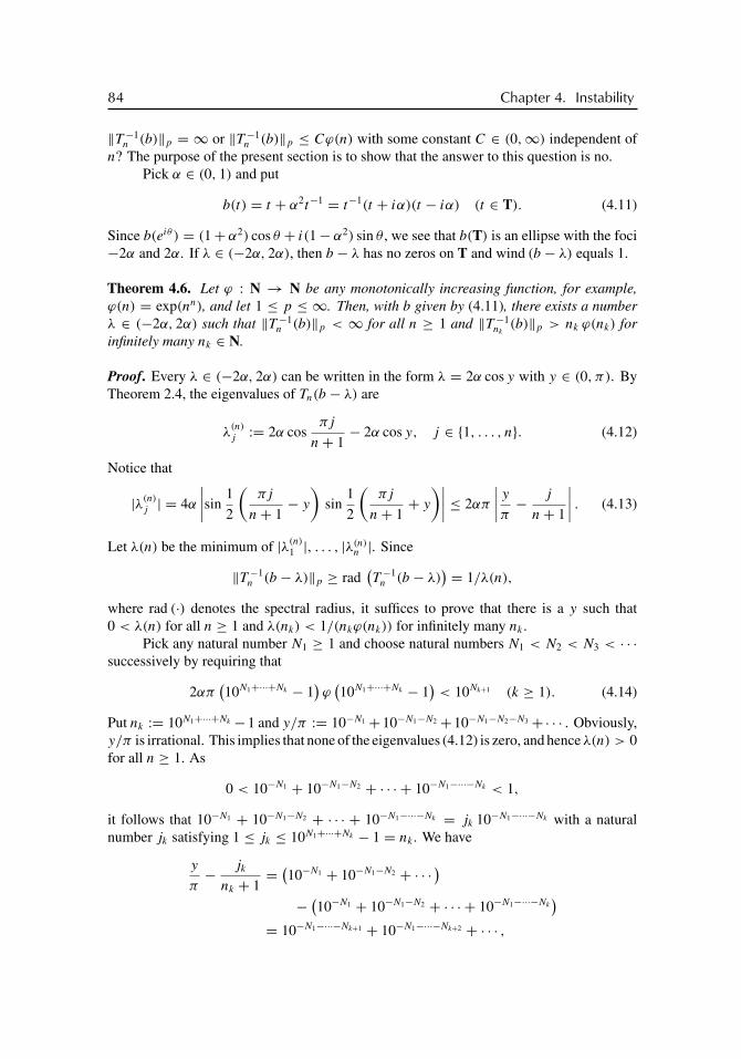
buch72005/10/5page 84

�

�

�

�

�

�

�

�


‖T −1n (b)‖p = ∞ or ‖T −1

n (b)‖p ≤ Cϕ(n) with some constant C ∈ (0,∞) independent ofn? The purpose of the present section is to show that the answer to this question is no.

Pick α ∈ (0, 1) and put

b(t) = t + α2t−1 = t−1(t + iα)(t − iα) (t ∈ T). (4.11)

Since b(eiθ ) = (1+ α2) cos θ + i(1− α2) sin θ , we see that b(T) is an ellipse with the foci−2α and 2α. If λ ∈ (−2α, 2α), then b − λ has no zeros on T and wind (b − λ) equals 1.

Theorem 4.6. Let ϕ : N → N be any monotonically increasing function, for example,ϕ(n) = exp(nn), and let 1 ≤ p ≤ ∞. Then, with b given by (4.11), there exists a numberλ ∈ (−2α, 2α) such that ‖T −1

n (b)‖p < ∞ for all n ≥ 1 and ‖T −1nk

(b)‖p > nk ϕ(nk) forinfinitely many nk ∈ N.

Proof. Every λ ∈ (−2α, 2α) can be written in the form λ = 2α cos y with y ∈ (0, π). ByTheorem 2.4, the eigenvalues of Tn(b − λ) are

λ(n)j := 2α cos

πj

n+ 1− 2α cos y, j ∈ {1, . . . , n}. (4.12)

Notice that

|λ(n)j | = 4α

∣∣∣∣sin1

2

(πj

n+ 1− y

)sin

1

2

(πj

n+ 1+ y

)∣∣∣∣ ≤ 2απ

∣∣∣∣ y

π− j

n+ 1

∣∣∣∣ . (4.13)

Let λ(n) be the minimum of |λ(n)1 |, . . . , |λ(n)

n |. Since

‖T −1n (b − λ)‖p ≥ rad

(T −1

n (b − λ)) = 1/λ(n),

where rad (·) denotes the spectral radius, it suffices to prove that there is a y such that0 < λ(n) for all n ≥ 1 and λ(nk) < 1/(nkϕ(nk)) for infinitely many nk .

Pick any natural number N1 ≥ 1 and choose natural numbers N1 < N2 < N3 < · · ·successively by requiring that

2απ(10N1+···+Nk − 1

)ϕ(10N1+···+Nk − 1

)< 10Nk+1 (k ≥ 1). (4.14)

Put nk := 10N1+···+Nk −1 and y/π := 10−N1 +10−N1−N2 +10−N1−N2−N3 +· · · . Obviously,y/π is irrational. This implies that none of the eigenvalues (4.12) is zero, and hence λ(n) > 0for all n ≥ 1. As

0 < 10−N1 + 10−N1−N2 + · · · + 10−N1−···−Nk < 1,

it follows that 10−N1 + 10−N1−N2 + · · · + 10−N1−···−Nk = jk 10−N1−···−Nk with a naturalnumber jk satisfying 1 ≤ jk ≤ 10N1+···+Nk − 1 = nk . We have

y

π− jk

nk + 1= (

10−N1 + 10−N1−N2 + · · · )− (

10−N1 + 10−N1−N2 + · · · + 10−N1−···−Nk)

= 10−N1−···−Nk+1 + 10−N1−···−Nk+2 + · · · ,

buch72005/10/5page 85

�

�

�

�

�

�

�

�

4.4. Sequences Versus Polynomials 85

which shows that

0 <y

π− jk

nk + 1< 2 · 10−N1−···−Nk+1 < 10−Nk+1 <

1

απ nkϕ(nk),

the last inequality resulting from (4.14). Thus, by (4.13),

λ(n) ≤∣∣∣λ(n)

jk

∣∣∣ < απ/(απ nkϕ(nk)) = 1/(nkϕ(nk)).

In Figure 4.2 we see plots of ‖T −1n (b− λ)‖2 for b(t) = t + 0.49 t−1 and six different

choices of λ (λ = 1.4 and λ = 0.01 in the top, λ = 0 and λ = 0.7 in the middle, andλ = 0.06 and λ = 1.294 in the bottom). If ‖T −1

n (b − λ)‖2 exceeded 1015, we plotted thevalue 1017.

4.4 Sequences Versus PolynomialsThis section serves as the preparation of the remaining sections of this chapter, which aredevoted to the growth of ‖T −1

n (b − λ)‖2 in case λ belongs to spessT (b) = b(T).In Section 1.6, we identified �2 with the Hardy space H 2. In what follows, it will be

convenient to identify �2n (= the linear space Cn with the �2 norm) with the space P+n of all

analytic polynomials of degree at most n − 1. Thus, with x = (x0, x1, . . . , xn−1) ∈ �2n we

associate the polynomial

f (eiθ ) = x0 + x1eiθ + · · · + xn−1e

i(n−1)θ . (4.15)

The scalar product and the norm in P+n are those of L2 = L2(T):

(f, g) =∫ 2π

0f (eiθ )g(eiθ )

dθ

2π, ‖f ‖2

2 =∫ 2π

0|f (eiθ )|2 dθ

2π.

Lemma 4.7. Let a ∈ W . If x, y ∈ �2n and f, g are the corresponding polynomials in P+n ,

then

(Tn(a)x, y) = 1

2π

∫ 2π

0a(eiθ )f (eiθ )g(eiθ ) dθ. (4.16)

In particular,

(Tn(a)x, x) = 1

2π

∫ 2π

0a(eiθ )|f (eiθ )|2 dθ, (4.17)

‖x‖2 = ‖f ‖2. (4.18)

Proof. We have∫ 2π

0a(eiθ )f (eiθ )g(eiθ ) dθ =

∫ 2π

0

(∑�

a�ei�θ

)(∑k

xkeikθ

)⎛⎝∑j

yj e−ijθ

⎞⎠ dθ

=∑�,j,k

a�xkyj

∫ 2π

0ei(�+k−j)dθ = 2π

∑j,k

aj−kxkyj = 2π(Tn(a)x, y).

buch72005/10/5page 86

�

�

�

�

�

�

�

�


0 20 40 60 80 10010

0

105

1010

1015

0 20 40 60 80 10010

0

105

1010

1015

0 20 40 60 80 10010

0

105

1010

1015

1020

0 20 40 60 80 10010

0

105

1010

1015

1020

0 20 40 60 80 10010

0

105

1010

1015

0 20 40 60 80 10010

0

105

1010

1015

1020

Figure 4.2. The norms ‖T −1n (b − λ)‖2 against n for b(t) = t + 0.49 t−1 and six

different choices of λ.

buch72005/10/5page 87

�

�

�

�

�

�

�

�

4.4. Sequences Versus Polynomials 87

Lemma 4.8. If a ∈ W and if x ∈ �2n and f ∈ P+n are related by (4.15), then

‖Tn(a)x‖2 ≤ ‖af ‖2. (4.19)

Proof. The j th Fourier coefficient of af is∑n−1

k=0 aj−kxk . As the map (1.17) is an isometry,we therefore get

‖af ‖22 =

∞∑j=−∞

∣∣∣∣∣n−1∑k=0

aj−kxk

∣∣∣∣∣2

≥n−1∑j=0

∣∣∣∣∣n−1∑k=0

aj−kxk

∣∣∣∣∣2

= ‖Tn(a)x‖22.

Lemma 4.9. If a ∈ W and f ∈ P+n , then ‖T −1n (a)‖2 ≥ ‖f ‖2/‖af ‖2.

Proof. By the definition of the norm,

‖T −1n (a)‖2 = sup

x �=0

‖T −1n (a)x‖2

‖x‖2= sup

y �=0

‖y‖2

‖Tn(a)y‖2.

Hence, if y ∈ �2n corresponds to f ∈ P+n , then ‖T −1

n (a)‖2 ≥ ‖y‖2/‖Tn(a)y‖2. From (4.18)and (4.19) we finally get ‖y‖2/‖Tn(a)y‖2 ≥ ‖f ‖2/‖af ‖2.

A class of good test polynomials. For j, m ∈ N, consider the Laurent polynomial

pjm(eiθ ) = (

1+ eiθ + · · · + eimθ)j

. (4.20)

Obviously,

pjm(eiθ ) =

(1− ei(m+1)θ

1− eiθ

)j

= eimjθ/2

(sin m+1

2 θ

sin θ2

)j

. (4.21)

From (4.20) we see that pjm ∈ P+mj+1. Both (4.20) and (4.21) immediately show that

‖pjm‖∞ = (m+ 1)j .

From (4.18) we deduce that

‖p1m‖2

2 = 12 + · · · + 12 = m+ 1. (4.22)

The following lemma gives good estimates for ‖pjm‖2 in the case j ≥ 2.

Lemma 4.10. For each j ≥ 1, there is a constant Dj ∈ (0,∞) such that

(1/Dj ) m2j−1 ≤ ‖pjm‖2

2 ≤ Dj m2j−1.

Proof. For j = 1, this follows from (4.22). So let j ≥ 2. Then

2π ‖pjm‖2

2 =∫ π

−π

(sin((m+ 1)θ/2)

θ/2

)2j (θ/2

sin(θ/2)

)2j

dθ

=∫ π

−π

(sin((m+ 1)θ/2)

θ/2

)2j (1+O(θ2)

)dθ,

buch72005/10/5page 88

�

�

�

�

�

�

�

�


and the substitution x = (m+ 1)θ/2 gives∫ π

−π

(sin((m+ 1)θ/2)

θ/2

)2j

O(θ2)dθ

= O

(8(m+ 1)2j−3

∫ π(m+1)/2

−π(m+1)/2

(sin x

x

)2j

x2dx

)= O

(m2j−3

)and ∫ π

−π

(sin((m+ 1)θ/2)

θ/2

)2j

dθ = 2(m+ 1)2j−1∫ π(m+1)/2

−π(m+1)/2

(sin x

x

)2j

dx

= 2(m+ 1)2j−1

(∫ ∞

−∞

(sin x

x

)2j

dx + o(1)

).

This shows that

limm→∞m−(2j−1)‖pj

m‖22 =

1

π

∫ ∞

−∞

(sin x

x

)2j

dx.

4.5 Symbols with Zeros: Lower EstimatesLet b be a Laurent polynomial. We now consider ‖T −1

n (b−λ)‖2 for λ ∈ spessT (b) = b(T).Equivalently, we study the behavior of ‖T −1

n (b)‖2 in the case where b has zeros on T.So suppose b(t0) = 0 for some t0 = eiθ0 ∈ T. Also assume that b does not vanish

identically. The function b is analytic in C \ {0}, and there is a smallest natural numberα ≥ 1 such that the αth derivative b(α)(t0) is nonzero. We then have

b(z) = b(α)(t0)

α! (z− t0)α +O

((z− t0)

α+1)

as z ∈ C approaches t0. We call α the order of the zero t0. Clearly, if b has a zero of orderα at t0, then

|b(t)| ≤ K|t − t0|α for all t ∈ T

and hence

|b(eiθ )| ≤ K|θ − θ0|α for all θ ∈ R

with some constant K ∈ (0,∞).

Theorem 4.11. Let b be a Laurent polynomial and suppose that b has a zero of order α att0 ∈ T. Then there is a constant C ∈ (0,∞) independent of n such that ‖T −1

n (b)‖2 ≥ C nα

for all n ≥ 1.

Proof. Put c(t) = b(t/t0) (t ∈ T). Then

Tn(c) = diag (1, t−10 , . . . , t

−(n−1)0 ) Tn(b) diag (1, t0, . . . , t

n−10 ),

buch72005/10/5page 89

�

�

�

�

�

�

�

�

4.5. Symbols with Zeros: Lower Estimates 89

whence ‖T −1n (b)‖2 = ‖T −1

n (c)‖2. Thus, we may assume without loss of generality thatt0 = 1. Then |b(eiθ )| ≤ K |θ |α for all θ ∈ R. Let n ≥ α + 2. There is a unique m ∈ Nsuch that n = m(α + 1)+ k with k ∈ {1, . . . , α + 1}. We show that

‖bpα+1m ‖2

2 / ‖pα+1m ‖2

2 ≤ D m−2α (4.23)

for some constant D ∈ (0,∞) independent of m. Since pα+1m belongs to P+n and m ≥

(n− α − 1)/(α + 1), the assertion then follows from Lemma 4.9.We have

2π ‖bpα+1m ‖2

2 =∫ π

−π

|b(eiθ )|2 |pα+1m (eiθ )|2dθ.

Since ‖pα+1m ‖∞ = (m+ 1)α+1, it follows that∫ 1/m

−1/m

|b(eiθ )|2 |pα+1m (eiθ )|2dθ ≤ K2 1

m2α(m+ 1)2α+2

∫ 1/m

−1/m

dθ ≤ M1m

with some M1 <∞ independent of m. As

|pα+1m (eiθ )|2 <

(sin

θ

2

)−(2α+2)

<(π

θ

)2α+2

for 0 < |θ | < π , we get∫1/m<|θ |<π

|b(eiθ )|2 |pα+1m (eiθ )|2dθ < 2K2

∫ π

1/m

θ2α(π/θ)2α+2dθ

= 2K2π2α+2∫ π

1/m

θ−2dθ < 2K2π2α+2 1

m2

∫ π

1/m

dθ ≤ M2 <∞.

Thus,

‖bpα+1m ‖2

2 ≤ M1m+M2 ≤ (M1 +M2)m. (4.24)

From Lemma 4.10 we know that

‖pα+1m ‖2

2 ≥ (1/Dα+1) m2α+1. (4.25)

Combining (4.24) and (4.25) we arrive at (4.23).

Corollary 4.12. Let b be a Laurent polynomial and assume the zeros of b on T are t1, . . . , tkwith the orders α1, . . . , αk . Then

‖T −1n (b)‖2 ≥ C nmax(α1,...,αk) for all n ≥ 1,

where C ∈ (0,∞) is a constant independent of n.

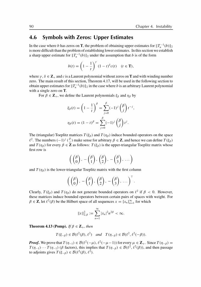
buch72005/10/5page 90

�

�

�

�

�

�

�

�


4.6 Symbols with Zeros: Upper EstimatesIn the case where b has zeros on T, the problem of obtaining upper estimates for ‖T −1

n (b)‖2

is more difficult than the problem of establishing lower estimates. In this section we establisha sharp upper estimate for ‖T −1

n (b)‖2 under the assumption that b is of the form

b(t) =(

1− 1

t

)γ

(1− t)δc(t) (t ∈ T),

where γ, δ ∈ Z+ and c is a Laurent polynomial without zeros on T and with winding numberzero. The main result of this section, Theorem 4.17, will be used in the following section toobtain upper estimates for ‖T −1

n (b)‖2 in the case where b is an arbitrary Laurent polynomialwith a single zero on T.

For β ∈ Z+, we define the Laurent polynomials ξβ and ηβ by

ξβ(t) =(

1− 1

t

)β

=β∑

j=0

(−1)j(

β

j

)t−j ,

ηβ(t) = (1− t)β =β∑

j=0

(−1)j(

β

j

)t j .

The (triangular) Toeplitz matrices T (ξβ) and T (ηβ) induce bounded operators on the space�2. The numbers (−1)j (

βj ) make sense for arbitrary β ∈ Z, and hence we can define T (ξβ)

and T (ηβ) for every β ∈ Z as follows: T (ξβ) is the upper-triangular Toeplitz matrix whosefirst row is ((

β

0

), −

(β

1

),

(β

2

), −

(β

3

), . . .

)and T (ηβ) is the lower-triangular Toeplitz matrix with the first column((

β

0

), −

(β

1

),

(β

2

), −

(β

3

), . . .

)�.

Clearly, T (ξβ) and T (ηβ) do not generate bounded operators on �2 if β < 0. However,these matrices induce bounded operators between certain pairs of spaces with weight. Forβ ∈ Z, let �2(β) be the Hilbert space of all sequences x = {xn}∞n=1 for which

‖x‖22,β :=

∞∑n=1

|xn|2n2β <∞.

Theorem 4.13 (Pomp). If β ∈ Z+, then

T (ξ−β) ∈ B(�2(β), �2) and T (η−β) ∈ B(�2, �2(−β)).

Proof. We prove that T (η−1) ∈ B(�2(−μ), �2(−μ−1)) for every μ ∈ Z+. Since T (η−β) =T (η−1) · · · T (η−1) (β factors), this implies that T (η−β) ∈ B(�2, �2(β)), and then passageto adjoints gives T (ξ−β) ∈ B(�2(β), �2).

buch72005/10/5page 91

�

�

�

�

�

�

�

�

4.6. Symbols with Zeros: Upper Estimates 91

For x = {xn}∞n=1 ∈ �2(−μ),

T (η−1)x =

⎛⎜⎜⎝11 11 1 1. . . . . . . . . . . .

⎞⎟⎟⎠⎛⎜⎜⎝

x1

x2

x3

. . .

⎞⎟⎟⎠ =

⎛⎜⎜⎝x1

x1 + x2

x1 + x2 + x3

. . .

⎞⎟⎟⎠ ,

whence

‖T (η−1)x‖22,−μ−1 = |x1|2 + |x1 + x2|2 1

22μ+2+ |x1 + x2 + x3|2 1

32μ+2+ · · ·

≤ |x1|2 + 1

22

( |x1|2μ

+ |x2|2μ

)2

+ 1

32

( |x1|3μ

+ |x2|3μ

+ |x3|3μ

)2

+ · · ·

≤ |x1|2 + 1

22

(|x1| + |x2|

2μ

)2

+ 1

32

(|x1| + |x2|

2μ+ |x3|

3μ

)2

+ · · · . (4.26)

Using Hardy’s inequality, which says that

a21 +

(a1 + a2

2

)2

+(

a1 + a2 + a3

3

)2

+ · · · ≤ 4(a2

1 + a22 + a2

3 + · · ·)

for every sequence {a1, a2, a3, . . . } of nonnegative numbers, we obtain that (4.26) does notexceed

4

(|x1|2 + |x2|2

22μ+ |x3|2

32μ+ · · ·

)= 4‖x‖2

2,−μ.

This proves that the operator T (η−1) : �2(−μ) → �2(−μ− 1) is bounded (and of norm atmost 2).

For β ∈ Z+, we put

Mβ = diag(μ

(β)

0 , μ(β)

1 , μ(β)

2 , . . .)

with μ(β)n :=

(β + n

n

).

By a theorem of Weierstrass,

∞∏k=1

(1+ β

k

)e−β/k = e−CE β

β! , (4.27)

where CE = 0.577 . . . is Euler’s constant. Since

1

1+ 1

2+ · · · + 1

n= CE + log n+ o(1),

(4.27) implies that there is a constant Dβ ∈ (1,∞) such that

(1/Dβ) nβ ≤ |μ(β)n | ≤ Dβ nβ for all n ≥ 1. (4.28)

buch72005/10/5page 92

�

�

�

�

�

�

�

�


Theorem 4.14 (Duduchava and Roch). If γ, δ ∈ Z+, then

T (ηγ )Mγ+δT (ξδ) = �γ,δMδT (ξδηγ )Mγ , (4.29)

where �γ,δ = γ !δ!/(γ + δ)!.

This is a set of nontrivial identities for binomial coefficients, and we invite the reader to tryhis or her hands. A full proof can be found in [70, Theorem 6.20]).

Corollary 4.15. If γ, δ ∈ Z+, then Tn(ξδηγ ) is invertible for all n ≥ 1 and there is aconstant C = Cγ,δ ∈ (0,∞) such that

‖T −1n (ξδηγ )‖2 ≤ C nγ+δ for all n ≥ 1.

Proof. Let �2n(β) be the space Cn with the �2(β) norm and let Mβ,n denote the operator

PnMβPn|Im Pn. On multiplying (4.29) from the left and the right by Pn, we get

Tn(ηγ )Mγ+δ,nTn(ξδ) = �γ,δMδ,nTn(ξδηγ )Mγ,n. (4.30)

As det Tn(ξδ) = det Tn(ηγ ) = 1, it follows that det Tn(ξδηγ ) �= 0. Furthermore, from (4.30)we obtain that

T −1n (ξδηγ ) = �γ,δMγ,nTn(ξ−δ)M

−1γ+δ,nTn(η−γ )Mδ,n. (4.31)

Consequently,

‖T −1n (ξδηγ )‖2 = ‖T −1

n (ξδηγ )‖B(�2n,�

2n)

≤ |�γ,δ| ‖Mγ,n‖B(�2n,�

2n)‖Tn(ξ−δ)‖B(�2

n(δ),�2n)

× ‖M−1γ+δ,n‖B(�2

n(−γ ),�2n(δ))

‖Tn(η−γ )‖B(�2n,�

2n(−γ )) ‖Mδ,n‖B(�2

n,�2n).

Theorem 4.13 implies that

‖Tn(ξ−δ)‖B(�2n(δ),�

2n)= ‖PnT (ξ−δ)Pn‖B(�2

n(δ),�2n)= O(1),

‖Tn(η−γ )‖B(�2n,�

2n(−γ )) = ‖PnT (η−γ )‖B(�2

n,�2n(−γ )) = O(1),


‖Mγ,n‖B(�2n,�

2n)= O(nγ ), ‖Mδ,n‖B(�2

n,�2n)= O(nδ),

‖M−1γ+δ,n‖B(�2

n(−γ ),�2n(δ))

= O(1).

Thus, ‖T −1n (ξδηγ )‖2 = O(nγ+δ).

We now extend Corollary 4.15 to symbols of the form ξδηγ c. This will be done onthe basis of the following perturbation theorem.

Theorem 4.16. Suppose(a) X, Y, Z, U are Banach spaces and Pn (n = 1, 2, 3, . . . ) are projections that are

defined and bounded on each of the spaces X, Y, Z, U ;

buch72005/10/5page 93

�

�

�

�

�

�

�

�


(b) Z ⊂ Y and X ⊂ U , the embeddings being continuous;(c) A ∈ B(X, Y ) is invertible;(d) the operators An := PnAPn ∈ B(PnX, PnY ) are invertible for all sufficiently

large n and, for each z ∈ Z, ‖A−1n Pnz− A−1z‖U → 0 as n→∞;

(e) K ∈ K(U, Z);(f) A+K ∈ B(X, Y ) is invertible.

Then(g) the operators Pn(A+K)Pn ∈ B(PnX, PnY ) are invertible for all n large enough;(h) ‖(Pn(A+K)Pn)

−1Pnz− (A+K)−1z‖U → 0 as n→∞ for each z ∈ Z.

Proof. The operator I+A−1K is an invertible element of B(X): the inverse is (A+K)−1A.We claim that I + A−1K is also an invertible element of B(U). Since A−1K : U → U iscompact, it follows that I + A−1K is Fredholm of index zero on U . Thus, we must showthat I + A−1K has a trivial kernel in U . Let (I + A−1K)u = 0 for some u ∈ U . Then

u = −A−1Ku �⇒ u ∈ X �⇒ Au = −Ku �⇒ (A+K)u = 0,

and this gives u = 0, as desired.From (d) and (e) we conclude that I +A−1

n PnK converges to I +A−1K uniformly onU (also recall Proposition 3.2). Therefore, by what was proved in the preceding paragraph,I + A−1

n PnK is an invertible element of B(U) for all sufficiently large n, say n ≥ n0. LetBn ∈ B(U) denote the inverse operator:

Bn + BnA−1n PnK = I , Bn + A−1

n PnKBn = I. (4.32)

The second inequality of (4.32) implies that Bn ∈ B(X). It also shows that PnBnPn = BnPn.Thus, for y ∈ Y ,

Pn(A+K)PnBnA−1n Pny = AnBnA

−1n Pny + PnKBnA

−1n Pny

= AnBnA−1n Pny + (An − AnBn)A

−1n Pny = AnA

−1n Pny = Pny

and, for x ∈ X,

BnA−1n PnPn(A+K)Pnx = BnA

−1n PnAnx + BnA

−1n PnKPnx

= BnPnx + (I − Bn)Pnx = Pnx.

It results that Pn(A+K)Pn ∈ B(PnX, PnY ) is invertible for all n ≥ n0, which is assertion(g), and that BnA

−1n Pn = (I + A−1

n PnK)−1A−1n Pn ∈ B(PnY, PnX) is the inverse operator.

Now let z ∈ Z and n ≥ n0. Since (I + A−1K)−1A−1 ∈ B(Y, X) is the inverse ofA+K ∈ B(X, Y ), we get

‖(Pn(A+K)Pn)−1Pnz− (A+K)−1Pnz‖U

≤ ‖((I + A−1n PnK)−1 − (I + A−1K)−1)A−1

n Pnz‖U

+ ‖(I + A−1K)−1(A−1n Pnz− A−1z)‖U

≤ ‖(I + A−1n PnK)−1 − (I + A−1K)−1‖B(U) ‖A−1

n Pn‖B(Z,U) ‖z‖Z

+ ‖(I + A−1K)−1‖B(U) ‖A−1n Pnz− A−1z‖U . (4.33)

buch72005/10/5page 94

�

�

�

�

�

�

�

�


We already observed that ‖A−1n PnK − A−1K‖B(U) → 0 as n→∞. Consequently,

‖(I + A−1n PnK)−1 − (I + A−1K)−1‖B(U)

≤ 2 ‖(I + A−1K)−1‖B(U) ‖A−1n PnK − A−1K‖B(U)

for all sufficiently large n. Now assertion (h) is immediate from (4.32).

Theorem 4.17. Let γ, δ ∈ Z+ and let c be a Laurent polynomial without zeros on the unitcircle T and with winding number zero. Put b = ξδηγ c. Then Tn(b) is invertible for allsufficiently large n and there exists a constant C = Cγ,δ,c ∈ (0,∞) such that

‖T −1n (b)‖2 ≤ C nγ+δ

for all n large enough.

Proof. Let Y be the image of T (ξδ) : �2 → �2. It is readily verified that T (ξ1) and hence alsoT (ξδ) = (T (ξ1))

δ is injective on �2. Thus, on defining a norm in Y by ‖y‖Y := ‖T (ξ−δ)y‖2

we make Y become a Banach space and T (ξδ) : �2 → Y become an isometric isomorphism.Let further X be the linear space of all sequences x = {xn}∞n=1 of complex numbers for whichT (ηγ )x ∈ �2. Since T (ηγ )x = 0 can only occur if x = 0, through ‖x‖X := ‖T (ηγ )x‖2

a norm is given in X and T (ηγ ) is an isometric isomorphism of X onto �2. Finally, putZ = �2(δ) and U = �2(−γ ). Theorem 4.13 is equivalent to the statement that Z iscontinuously embedded in Y and that X is continuously embedded in U . At this point wehave assumption (b) of Theorem 4.16.

The usual projection Pn onto the first n coordinates is obviously bounded on Z andU , and it can be checked straightforwardly that Pn is also bounded on X and Y (notice thatwe do not require that supn ‖Pn‖ <∞). Thus, assumption (a) of Theorem 4.16 is also met.

Let c = c−c+ be a Wiener-Hopf factorization and put

A = T (c+)T (ξδηγ )T (c−), A+K = T (c−)T (ξδηγ )T (c+).

Note that A+K = T (b).We claim that the operators T (c±) are bounded and invertible on X and Y . Clearly,

T (c±) ∈ B(X) ⇐⇒ T (ηγ )T (c±)T (η−γ ) ∈ B(�2).

Since T (ηγ )T (c+)T (η−γ ) = T (c+), it is obvious that T (c+) ∈ B(X). The argument of theproof of Proposition 1.3 gives

T (ηγ )T (c−)T (η−γ ) = T (c−)−H(ηγ )H (c−)T (η−γ ).

The operator T (η−γ ) : �2 → �2(−γ ) is bounded due to Theorem 4.13. As H(ηγ ) and H(c−)

have only finitely many nonzero entries, we see that the linear operator H(ηγ )H (c−) :�2(−γ ) → �2 is also bounded. Consequently, T (c−) ∈ B(X). Analogously, T (c−1

± ) ∈B(X). This shows that the operators T (c±) are invertible on X. The boundedness andinvertibility of T (c±) on Y can be proved similarly.

buch72005/10/5page 95

�

�

�

�

�

�

�

�


The result of the previous paragraph in conjunction with the equality T (ξδηγ ) =T (ξδ)T (ηγ ) reveals that A and A + K are bounded and invertible as operators from X toY . Thus, we have assumptions (c) and (f) of Theorem 4.16. By Proposition 1.3,

K = T (c+ξδηγ c−)− T (c+)T (ξδηγ )T (c−)

= T (c+)H(ξδηγ )H (c−)+H(c+)H (ξδηγ c+),

and since the Hankel operators have at most a finite number of nonzero entries, we concludethat assumption (e) of Theorem 4.16 is also satisfied.

We are left with the verification of assumption (f) of Theorem 4.16. We have

An = PnT (c+)T (ξδηγ )T (c−)Pn = Tn(c+)Tn(ξδηγ )Tn(c−).

From Corollary 4.15 we therefore deduce that An is invertible for all sufficiently large n andthat

A−1n = Tn(c

−1− )T −1

n (ξδηγ )Tn(c−1+ ) = T (c−1

− )PnT−1n (ξδηγ )PnT (c−1

+ ).

Consequently, since A−1 = T (c−1− )T (η−γ )T (ξ−δ)T (c−1

+ ), assumption (f) will follow assoon as we have shown that

‖T −1n (ξδηγ )Pnz− T (η−γ )T (ξ−δ)z‖2,−γ → 0 as n→∞

for every z ∈ �2(δ). Formulas (4.31) and (4.29) give

T −1n (ξδηγ ) = �γ,δMγ PnT (ξ−δ)PnM

−1γ+δPnT (η−γ )PnMδ

= �γ,δMγ T (ξ−δ)M−1γ+δPnT (η−γ )Mδ

and

T (η−γ )T (ξ−δ) = �γ,δMγ T (ξ−δ)M−1γ+δT (η−γ )Mδ.

Thus, with μ := |�γ,δ| and constants Cj ∈ (0,∞),

‖T −1n (ξδηγ )Pnz− T (η−γ )T (ξ−δ)z‖2,−γ

= μ ‖Mγ T (ξ−δ)M−1γ+δQnT (η−γ )Mδz‖2,−γ

≤ μ C1 ‖T (ξ−δ)M−1γ+δQnT (η−γ )Mδz‖2 (by (4.28))

≤ μ C2 ‖M−1γ+δQnT (η−γ )Mδz‖2,δ (by Theorem 4.13)

≤ μ C3 ‖QnT (η−γ )Mδz‖2,−γ (by (4.28)).

Since T (η−γ )Mδz ∈ �2(−γ ) by virtue of Theorem 4.13 and (4.28) and since Qn convergesstrongly to zero on �2(−γ ), it follows that ‖QnT (η−γ )Mδz‖2,−γ → 0, as desired.

Theorem 4.16 now gives that ‖(Pn(A + K)Pn)−1Pnz − (A + K)−1z‖2,−γ → 0 as

n→∞ for every z ∈ �2(δ). Hence, by Theorem 3.1,

supn

‖T −1n (b)‖B(�2

n(δ),�2n(−γ )) = sup

n

‖(Pn(A+K)Pn)−1‖B(�2

n(δ),�2n(−γ )) <∞.

buch72005/10/5page 96

�

�

�

�

�

�

�

�


Because

‖H‖2 = ‖H‖B(�2n,�

2n)≤ nγ+δ ‖H‖B(�2

n(δ),�2n(−γ ))

for every n× n matrix H , we finally get ‖T −1n (b)‖2 = O(nγ+δ).

Given two sequences {αn}∞n=1 and {βn}∞n=1 of positive numbers, we write αn � βn

if there exists a constant C ∈ (1,∞) such that (1/C)βn ≤ αn ≤ Cβn for all sufficientlylarge n. Combining Theorems 4.11 and 4.17 we arrive at the conclusion that if b = ξδηγ c

with a Laurent polynomial c that has no zeros on T and has winding number zero, then‖T −1

n (b)‖2 � nγ+δ .

4.7 Inside the Essential SpectrumThroughout this section we assume that b is a Laurent polynomial. We study the behaviorof ‖T −1

n (b − λ)‖2 in the case where λ ∈ spessT (b) = b(T).Clearly, λ ∈ b(T) if and only if b − λ has zeros on T. We denote by S(b) the points

λ for which b − λ has at least two distinct zeros on T. The points in S(b) are met at leasttwice by b(t) as t traces out the unit circle T. If λ ∈ b(T) \ S(b), then b(T) is an (analytic)arc in a sufficiently small neighborhood of λ.

Theorem 4.18. Let λ ∈ b(T) \ S(b) and

b(t)− λ = (t − t0)βtkc(t), t ∈ T, (4.34)

where β ∈ N, k ∈ Z, c(t) �= 0 for t ∈ T, and wind (c, 0) = 0. Then

‖T −1n (b − λ)‖2 � nβ if −β ≤ k ≤ 0, (4.35)

and there are constants C ∈ (0,∞) and α ∈ (0,∞) such that

‖T −1n (b − λ)‖2 ≥ C eαn if k < −β or k > 0. (4.36)

Proof. Theorem 4.11 shows that the inequality ‖T −1n (b−λ)‖2 ≥ C nβ is true in either case.

Suppose first that −β ≤ k ≤ 0. We then can write

b(t)− λ =(

1− t

t0

)β−|k| (1− t0

t

)|k|(−t0)

β−|k|c(t)

with β − |k| ≥ 0 and |k| ≥ 0. Consequently, by Theorem 4.17,

‖T −1n (b − λ)‖2 = O(nβ−|k|+|k|) = O(nβ).

This in conjunction with Theorem 4.11 completes the proof of (4.35).Now suppose k < −β or k > 0. Since

b(t)− λ := b(1/t)− λ = (1− t0t)β t−β−kc(1/t), t ∈ T,

buch72005/10/5page 97

�

�

�

�

�

�

�

�

4.7. Inside the Essential Spectrum 97

and ‖T −1n (b − λ)‖2 = ‖T −1

n (b − λ)‖2, it suffices to consider the case k < −β. Thus, letk = −β − m with m > 0. Let c = c−c+ be the Wiener-Hopf factorization introduced inthe proof of Theorem 4.1 and define x and x(n) as in that proof. We have

b(t)− λ = (t − t0)βt−β−mc−(t)c+(t) =

(1− t0

t

)β

t−mc−(t)c+(t),

which can be written in the form b(t)− λ = ξβ(t)χ−m(t)c−(t)c+(t). As T (c+)x = e0 andm > 0, it results that PnT (b − λ)x = PnT (ξβc−)T (χ−m)T (c+)x = 0. Hence, again as inthe proof of Theorem 4.1,

‖Tn(b − λ)x(n)‖2 = ‖PnT (b − λ)x(n)‖2 = ‖PnT (b − λ)(x(n) − x)‖2

≤ ‖T (b − λ)‖2‖x(n) − x‖2 ≤ D e−αn

with certain constants D, α ∈ (0,∞), which yields (4.36).

Example 4.19. Consider the symbol b(t) = (t − 1)2tk(2.001 + t + 0.49t−1). Figure 4.3shows what happens in the five cases k = −3,−2,−1, 0, 1. In each picture we see thenorm ‖T −1

n (b)‖2 against n. We also plotted the shape of the curve b(T) in the lower-rightcorner; the origin is marked by a big dot. As predicted by Theorem 4.18, the norms increaseat least exponentially for k = −3 and k = 1, while the growth of the norms is polynomialfor −2 ≤ k ≤ 0. In the picture in the bottom, we replaced values greater than 1015 by thevalue 1017.

Our next objective is to translate Theorem 4.18 into geometrical language. We labeleach connected component of C \ b(T) by the winding number of the oriented curve b(T)

about the points of the component. Let λ ∈ b(T)\S(b). Then there is an open neighborhoodUλ ⊂ C of λ such that Uλ ∩ b(T) =: γλ is an oriented analytic arc. Clearly, λ belongs tothe boundaries of exactly two components �+

λ and �−λ of C \ b(T). We let �+

λ stand forthe component on the left of γλ, and, accordingly, �−

λ is the component on the right of γλ.

Lemma 4.20. Let λ ∈ b(T) \ S(b). If m is the winding number of �+λ , then �−

λ has thewinding number m− 1.

Proof. Let n be the winding number of �−λ . Fix a sufficiently small disk Uλ centered at λ,

pick a point μ ∈ Uλ ∩�+λ , and replace b(T) by the continuous curve δλ that coincides with

b(T) outside Uλ and with ∂Uλ∩�+λ otherwise. It is obvious that wind (δλ, μ) = m−1. On

the other hand, since μ and �−λ are contained in the same connected component of C \ δλ,

we have wind (δλ, μ) = n. Consequently, n = m− 1.

For r ∈ (0, 1), put br(t) = b(rt) (t ∈ T).

Lemma 4.21. Let λ ∈ b(T) \S(b) and let β be the order of the zero of b−λ on T. Supposer ∈ (0, 1) is sufficiently close to 1 and a point moves along the curve br(T), following theorientation of this curve. Then, in a small neighborhood Uλ ⊂ C of λ, this point is firstin �+

λ ∩ Uλ, then it encircles λ exactly [(β − 1)/2] times in the clockwise direction, afterwhich it is again in �+

λ ∩ Uλ.

buch72005/10/5page 98

�

�

�

�

�

�

�

�


0 20 40 60 8010

0

105

1010

1015

k = −3

0 20 40 60 8010

0

101

102

103

k = −2

0 20 40 60 8010

0

101

102

103

k = −1

0 20 40 60 8010

0

101

102

103

k = 0

0 20 40 60 8010

0

105

1010

1015

1020

k = 1

Figure 4.3. Norms ‖T −1n (b)‖2 for several symbols b with zeros.

buch72005/10/5page 99

�

�

�

�

�

�

�

�

4.7. Inside the Essential Spectrum 99

Proof. This follows from the fact that the Riemann surface of b(z)− λ at z = t0 is locallyhomeomorphic to the Riemann surface of zβ at the origin and that rT lies “on the left” ofthe circle T.

Theorem 4.22. Let λ ∈ b(T) \ S(b). Suppose the order of the zero of b − λ is β and thewinding number of �+

λ is m. Then

‖T −1n (b − λ)‖2 � nβ if −

[β

2

]≤ m ≤

[β + 1

2

], (4.37)

and there are constants C ∈ (0,∞) and α ∈ (0,∞) such that

‖T −1n (b − λ)‖2 ≥ C eαn if m < −

[β

2

]or m >

[β + 1

2

]. (4.38)

Proof. Write b − λ in the form (4.34). Then b(rt)− λ = (rt − t0)βrktkc(rt) for t ∈ T. If

r ∈ (0, 1) is sufficiently close to 1, then λ /∈ br(T) and

wind (b(rt), λ) = wind (b(rt)− λ, 0)

= wind ((rt − t0)β, 0)+ k + wind (c(rt), 0) = 0+ k + 0 = k.

Evidently, ‖br − b‖∞ → 0 as r → 1− 0. This in conjunction with Lemma 4.21 shows thatif μ ∈ �−

λ is sufficiently close to λ, then

wind (b(rt), λ) = wind (b(rt), μ) = wind (b(t), μ)−[β − 1

2

].

Consequently, k = wind (b, μ) − [(β − 1)/2]. By Lemma 4.20, wind (b, μ) = m − 1. Itresults that k = m− 1− [(β − 1)/2], and since

−β ≤ m− 1−[β − 1

2

]≤ 0 ⇐⇒ −

[β

2

]≤ m ≤

[β + 1

2

],

(4.37) and (4.38) follow from (4.35) and (4.36).

Here are two interesting special cases. Recall that, by Corollary 1.12,

sp T (b) = b(T) ∪{λ ∈ C \ b(T) : wind (b, λ) �= 0

}.

Corollary 4.23. If λ ∈ b(T) \ S(b) is located on ∂ sp T (b), the boundary of the spectrumof T (b), and β is the order of the zero of b − λ, then

‖T −1n (b − λ)‖2 � nβ.

Proof. By assumption, �+λ or �−

λ has the winding number zero. From Lemma 4.20 wededuce that the winding number m of �+

λ is 0 or 1. Since [(β+1)/2)] ≥ 1 and−[β/2] ≤ 0for every β ∈ N, the assertion follows from (4.37).

Corollary 4.24. If λ belongs to b(T) \ S(b) and the order of the zero of b − λ is 1, then‖T −1

n (b−λ)‖2 � n for λ ∈ ∂ sp T (b), while ‖T −1n (b−λ)‖2 increases at least exponentially

in case λ /∈ ∂ sp T (b).

buch72005/10/5page 100

�

�

�

�

�

�

�

�


Proof. The first part of the assertion is immediate from Corollary 4.23. So suppose λ ∈b(T) \ (S(b) ∪ ∂ sp T (b)) and let m be the winding number of �+

λ . As neither �+λ nor �−

λ

have the winding number zero, we infer from Lemma 4.20 that m �= 0 and m − 1 �= 0.Consequently, m > 1 or m < 0, and Theorem 4.22 with β = 1 completes the proof.

Example 4.25. Let b(t) = (t + 1)3. We have b(T) = A ∪ {−1} ∪B ∪ {0}, where A and B

are as in Figure 4.4.

–2 –1 0 1 2 3 4 5 6 7 8 9–6

–4

–2

0

2

4

6

A

A

A

B

B

0 –1

Figure 4.4. The curve b(T) for b(t) = (t + 1)3.

Theorem 4.22 implies that

‖T −1n (b − λ)‖2 �

{n for λ ∈ A,

n3 for λ = 0,

and that ‖T −1n (b−λ)‖2 increases at least exponentially for λ ∈ B. We are left with λ = −1.

In that case

b(t)− λ = (t + 1)3 + 1 = (t2 + t + 1)(t + 2) = (t − ω)(t − ω2)(t + 2),

where ω = e2πi/3. Since the two zeros of b− λ on T are of order 1, Corollary 4.12 impliesthat ‖T −1

n (b − λ)‖2 ≥ C n with some constant C. The results we have established so farcannot be used to obtain an upper estimate for ‖T −1

n (b−λ)‖2. However, in the case at handwe can proceed as follows. Since

Tn(b(t)− λ) = Tn(t2 + t + 1)Tn(t + 2)

and supn ‖T −1n (t + 2)‖2 <∞ by Theorem 3.7, it remains to estimate the norms ‖T −1

n (t2 +t + 1)‖2 from above. It can be checked straightforwardly that T −1

n (t2 + t + 1) is thelower-triangular Toeplitz matrix whose first column is

( 1, −1, 0, 1, −1, 0, 1, −1, 0, . . . )�.

buch72005/10/5page 101

�

�

�

�

�

�

�

�

4.8. Semi-Definite Matrices 101

By computing the Frobenius norm of that matrix or by writing it as

Tn(1)+ Tn(−t)+ Tn(t3)+ Tn(−t4)+ Tn(t

6)+ Tn(−t7)+ · · · ,

we see that the spectral norm is O(n). In summary, ‖Tn(b − λ)‖2 � n for λ = −1.

Example 4.26. Things are very complicated for points λ ∈ S(b). Let, for example,b(t) − λ = t k(t − 1)(t + 1) (t ∈ T). Corollary 4.12 gives ‖T −1

n (b − λ)‖2 ≥ C n for alln ≥ 1. If k ≤ −3 or k ≥ 1, then Tn(b−λ) is triangular with zeros on the main diagonal andhence ‖T −1

n (b−λ)‖2 = ∞. In the case k = 0, the inverse of Tn(b−λ) is the lower-triangularToeplitz matrix with the first column

( −1, 0, −1, 0, −1, 0, . . . )�,

and as in Example 4.25 we obtain that the spectral norm of this matrix is O(n). Thus,‖T −1

n (b − λ)‖2 � n for k = 0. Passage to adjoints yields the same result for k = −2.Finally, let k = −1. Then Tn(b−λ) is a skew-symmetric tridiagonal Toeplitz matrix.

Thus, ‖T −1n (b − λ)‖2 = ∞ if n is odd. For even n we may employ the fact that Tn(b − λ)

is normal and hence ‖T −1n (b− λ)‖2 = 1/μn where μn is the minimum of the moduli of the

eigenvalues of Tn(b − λ). From Theorem 2.4 we infer that the eigenvalues of T2m(b − λ)

are 2i cos πj/(2m+ 1) (j = 1, . . . , 2m), which shows that

μ2m = 2 cosπm

2m+ 1= 2 sin

π

4m+ 2∼ 2π

4m+ 2∼ π

2m= π

n.

Consequently, ‖T −1n (b − λ)‖2 ∼ n/π for even n, where here and throughout the book

αn ∼ βn means that αn/βn → 1.

4.8 Semi-Definite MatricesA matrix A ∈ Cn×n is said to be positive semi-definite if Re (Ax, x) ≥ 0 for all x in Cn andis called positive definite if there is an ε > 0 such that Re (Ax, x) ≥ ε‖x‖2

2 for all x ∈ Cn.From (4.17) we infer that if a ∈ W and Re a(t) ≥ 0 for all t ∈ T, then Tn(a) is positivesemi-definite, and that if a ∈ W and Re a(t) ≥ ε > 0 for all t ∈ T, then Tn(a) is positivedefinite.

In this section we establish upper estimates for ‖T −1n (b)‖2 in terms of the zeros of the

real part Re b of b provided b is positive semi-definite, that is, in the case where Re b(t) ≥ 0for all t ∈ T. The estimates we will obtain are very coarse in general, but they have someadvantages. First, they imply that if b is a Laurent polynomial and λ ∈ ∂ conv b(T) then‖T −1

n (b−λ)‖2 grows at most polynomially; note that λ is allowed to belong to S(b). Second,our estimates for ‖T −1

n (b)‖2 are sharp in case b is real valued and nonnegative.For a ∈ W , let R(a) = a(T) be the range of a, let convR(a) stand for the convex hull

of R(a), let ∂ convR(a) denote the boundary of convR(a), and put dist (0, convR(a)) :=min{|z| : z ∈ convR(a)}.

Proposition 4.27. Suppose a ∈ W does not vanish identically and R(a) is not a linesegment containing the origin in its interior. If

0 /∈ convR(a) or 0 ∈ ∂ convR(a), (4.39)

buch72005/10/5page 102

�

�

�

�

�

�

�

�


then Tn(a) is invertible for all n ≥ 1.

Proof. Assume Tn(a) is not invertible. Then Tn(a)x = 0 for some x ∈ Cn \ {0}, and (4.17)implies that there exists a polynomial f ∈ P+n \ {0} such that

∫a|f |2 = 0. By (4.39), we

can find a number γ ∈ T such that Re (γ a) ≥ 0. As∫

Re (γ a)|f |2 = 0 and |f |2 > 0 almosteverywhere, it follows that Re (γ a) = 0 throughout T. Consequently, R(γ a) = i[m, M]with real numbers m < M . Since

∫Im (γ a)|f |2 = 0 and |f |2 > 0 almost everywhere, we

deduce that m < 0 and M > 0. However, this case was excluded.

Corollary 4.28. Let a ∈ W . If R(a) is a singleton, then sp Tn(a) = R(a). If R(a) is aline segment [z1, z2] with z1 �= z2, then

sp Tn(a) ⊂ [z1, z2] \ {z1, z2}. (4.40)

Finally, if R(a) is neither a singleton nor a line segment, then

sp Tn(a) ⊂ convR(a) \ ∂ convR(a). (4.41)

Proof. The case where R(a) is a singleton is trivial. The inclusion (4.41) is immediatefrom Proposition 4.27. We are so left with the case where R(a) is a proper line segment.From Proposition 4.27 we deduce that sp Tn(a) ⊂ [z1, z2]. Assume z1 is in sp Tn(a). Then,as in the proof of Proposition 4.27,

∫(a − z1)|f |2 = 0 for some nonzero f ∈ P+n . Since

R(γ (a − z1)) ⊂ [0,∞) for some γ ∈ T, we therefore see that a(t) = z1 for all t ∈ T,which means that R(a) is a singleton. Thus, z1 /∈ sp Tn(a). Analogously one can show thatz2 /∈ sp Tn(a).

Theorem 4.29 (Brown and Halmos). Let a ∈ W and suppose

d := dist (0, convR(a)) > 0. (4.42)

Then T (a) is invertible on �2 with

‖T −1(a)‖2 ≤ 1/d (4.43)

and Tn(a) is invertible for all n ≥ 1 with

‖T −1n (a)‖2 ≤ 1/d. (4.44)

Proof. There is a γ ∈ T such that the set γ convR(a) is contained in the half-plane{z ∈ C : Re z ≥ d}. Fix any ε ∈ (0, d). If r is sufficiently large, then the disk {z ∈ C :|z− (d+ r−ε)| < r} certainly contains the set γ convR(a). Thus |γ a(t)−d− r+ε| < r

for all t ∈ T and therefore ∣∣∣∣ γ a(t)

d + r − ε− 1

∣∣∣∣ <r

d + r − ε

for all t ∈ T. Since

γ

d + r − εT (a) = I + T

(γ a

d + r − ε− 1

)

buch72005/10/5page 103

�

�

�

�

�

�

�

�


and the norm of the Toeplitz operator on the right is less than r/(d + r − ε) < 1, it followsfrom expansion into the Neumann series that T (a) is invertible and that

d + r − ε

|γ | ‖T −1(a)‖2 <1

1− rd+r−ε

= d + r − ε

d − ε,

whence ‖T −1(a)‖2 < 1/(d− ε). As ε ∈ (0, d) can be chosen as small as desired, we arriveat estimate (4.43). Clearly, the argument remains true with T (a) replaced by Tn(a) and soalso gives (4.44).

Example 4.30. Consider the n× n Toeplitz matrix

Tn(b) =

⎛⎜⎜⎜⎜⎜⎝2 −1 0 . . . 0−1 2 −1 . . . 00 −1 2 . . . 0...

......

. . ....

0 0 0 . . . 2

⎞⎟⎟⎟⎟⎟⎠ .

The symbol is b(eiθ ) = −e−iθ + 2 − eiθ = 2(1 − cos θ). Obviously, R(b) = [0, 4] andhence d = dist (0, convR(b)) = 0. Thus, Theorem 4.29 is not applicable. However, let usreplace b by b + ign, where

gn(eiθ ) = cos nθ = (einθ + e−inθ )/2.

As the Fourier coefficients (gn)k of gn are zero for |k| ≤ n− 1, we have

Tn(b) = Tn(b + ign). (4.45)

Clearly, dn := dist (0, convR(b + ign)) > 0, and we can therefore apply Theorem 4.29 tothe matrices (4.45).

Our aim is to estimate dn from below. The graph of b + ign in C = R2 is given by

(2− 2 cos θ, cos nθ), θ ∈ (−π, π ]. (4.46)

Put

εn = 4

3

(1− cos

π

3n

)= 8

3sin2 π

6n. (4.47)

The graph of (2− 2 cos θ,

1

2− 1

εn

(2− 2 cos θ)

), θ ∈ R (4.48)

is the straight line y = 1/2 − (1/εn)x. We show that the range of b + ign lies above thisline. By (4.46) and (4.48) this is equivalent to showing that

1

εn

(2− 2 cos θ)+ cos nθ ≥ 1

2(4.49)

buch72005/10/5page 104

�

�

�

�

�

�

�

�


for θ ∈ (−π, π ]. If |nθ | < π/3, then cos nθ > 1/2 and hence (4.49) is true. If |nθ | ≥ π/3,then cos θ ≤ cos(π/(3n)), whence, by (4.47),

1

εn

(2− 2 cos θ)+ cos nθ ≥ 1

εn

(2− 2 cos

π

3n

)− 1 = 1

2,

which gives (4.49) again.Thus, dn ≥ Dn where Dn is the distance of the origin to the straight line y = 1/2 −

(1/εn)x. Obviously,

Dn = εn

4

1√1/4+ ε2

n/4.

Since εn → 0 as n→∞, we have Dn > εn/(2√

2 ) for all sufficiently large n. Taking intoaccount (4.44), (4.45), (4.47) we therefore obtain

‖T −1n (b)‖2 ≤ 1

dn

≤ 1

Dn

<2√

2

εn

= 3√

2

4

1

sin2(π/(6n))<

3√

2

4

(π

2

6n

π

)2

< 10 n2.

To extend the trick employed in this example to symbols with more than one zero, weneed a further result.

Lemma 4.31 (Dirichlet). Let β1, . . . , βN be real numbers and μ > 0. Then there existsa number q ∈ N such that 1 ≤ q ≤ ([1/μ] + 1)N and qβj ∈ Z + (−μ, μ) for allj ∈ {1, . . . , N}.

Proof. For x ∈ R, denote by {x} the fractional part of x. Thus, x = [x] + {x} with [x] ∈ Zand {x} ∈ [0, 1). Put K = [1/μ] + 1 and divide the cube [0, 1)N into KN congruent cubesof the form

[i1/K, (i1 + 1)/K)× · · · × [iN/K, (iN + 1)/K). (4.50)

The KN+1 points ({�β1}, . . . , {�βN }), � = 0, 1, . . . , KN all belong to [0, 1)N and thereforetwo of them must be located in the same cube (4.50). Consequently, there are �1, �2 suchthat 0 ≤ �1 < �2 ≤ KN and |{�2βj } − {�1βj }| < 1/K for all j . Put q = �2 − �1 andmj = [�2βj ] − [�1βj ]. Then

|qβj −mj | = |�2βj − [�2βj ] − (�1βj − [�1βj ])| = |{�2βj } − {�1βj }| < 1/K < μ.

Theorem 4.32. Let b be a Laurent polynomial and suppose 0 ∈ b(T). Assume that Re b ≥ 0on T and that Re b is not identically zero. Then Re b has a finite number of zeros on T andthe orders of these zeros are all even. If 2α is the maximal order of the zeros of Re b on T,then

‖T −1n (b)‖2 ≤ D n2α for all n ≥ 1

with some constant D ∈ (0,∞) independent of n.

buch72005/10/5page 105

�

�

�

�

�

�

�

�


Proof. Put u(θ) := Re b(eiθ ). Clearly, u is also a Laurent polynomial. By assumption, u

does not vanish identically, u(θ) ≥ 0 for all θ , and u has N ≥ 1 zeros θ1, . . . , θN ∈ (−π, π ]of even orders 2α1, . . . , 2αN . Since Tn(b) is invertible for all n ≥ 1 due to Proposition 4.27,it suffices to prove the estimate ‖T −1

n (b)‖2 ≤ D n2α for all n large enough.Using Lemma 4.31 with μ = 1/12 and βj = nθj/(2π), we get an integer qn such

that

1 ≤ qn ≤ 13N, nqnθj ∈ 2πZ+ (−π/6, π/6). (4.51)

We have

cos(nqnθ) = cos(nqnθj ) cos(nqn(θ − θj ))− sin(nqnθj ) sin(nqn(θ − θj )),


cos(nqnθj ) > cosπ

6=√

3

2, sin(nqnθj ) < sin

π

6= 1

2.

If |nqn(θ − θj )| < π/6, then

cos(nqn(θ − θj )) > cosπ

6=√

3

2, sin(nqn(θ − θj )) < sin

π

6= 1

2.

Hence,

cos(nqnθ) >

√3

2

√3

2− 1

2

1

2= 1

2for |θ − θj | < π

6nqn

. (4.52)

Choose δ > 0 so that the sets (θj − δ, θj + δ) are pairwise disjoint and put

1

ωj(n):= min

{u(θ) : 1

n≤ |θ − θj | < δ

}. (4.53)

Since θj is a zero of the order 2αj , there is a constant Cj ∈ (1,∞) such that

(1/Cj ) n2αj ≤ ωj(n) ≤ Cj n2αj . (4.54)

Let v(θ) := Im b(eiθ ) and put

1

εn,j

:= 3 (‖v‖∞ + 1) ωj

(6nqn

π

), M := 2 (‖v‖∞ + 1). (4.55)

Consider the function

an(eiθ ) := b(eiθ )+ i M cos(nqnθ).

Since qn ≥ 1, we have Tn(b) = Tn(an). Now let n be so large that π/(6nqn) < δ. Weclaim that the range R(an|(θj − δ, θj + δ)) lies above the straight line y = 1− x/εn,j . Asan(e

iθ ) = u(θ)+ i(v(θ)+M cos(nqnθ)), this is equivalent to claiming that

v(θ)+M cos(nqnθ) > 1− u(θ)/εn,j

buch72005/10/5page 106

�

�

�

�

�

�

�

�


for all θ ∈ (θj − δ, θj + δ). We prove that actually

u(θ)/εn,j +M cos(nqnθ) > 1+ ‖v‖∞ (4.56)

for all θ ∈ (θj − δ, θj + δ).If |θ − θj | < π/(6nqn), then (4.52), (4.54), and the nonnegativity of u(θ) give

u(θ)/εn,j +M cos(nqnθ) >m

2= ‖v‖∞ + 1.

So let π/(6nqn) ≤ |θ − θj | < δ. Then, by (4.53) and (4.55),

u(θ)/εn,j +M cos(nqnθ) ≥ 1

εn,j ωj (6nqn/π)−M

= 3 (‖v‖∞ + 1)− 2 (‖v‖∞ + 1) = ‖v‖∞ + 1.

This completes the proof of (4.56).Thus, the range of the restriction of an to

⋃j (θj − δ, θj + δ) lies above the line

y = 1− x/εn, εn := minj

εn,j (4.57)

(here we also took into account that Re an ≥ 0). The number η given by

η = inf

⎧⎨⎩u(θ) : θ ∈ (−π, π ]∖

N⋃j=1

(θj − δ, θj + δ)

⎫⎬⎭is positive. If θ ∈ (−π, π ] \⋃

j (θj − δ, θj + δ), then an(eiθ ) is located on the right of the

vertical line x = η. Since 1/εn →∞ as n →∞, it follows that R(an) is contained in thehalf-plane above the line (4.57) for all sufficiently large n.

The distance of the origin to the line (4.57) is Dn := εn/√

1+ ε2n. Thus, Dn > εn/2

if only n is large enough. From Theorem 4.29 and (4.55), (4.57) we now obtain that

‖T −1n (b)‖2 = ‖T −1

n (an)‖2 ≤ 1

Dn

<2

εn

= 6 (‖v‖∞ + 1) maxj

ωj

(6nqn

π

),

whence, by (4.51) and (4.54), ‖T −1n (b)‖2 = O(nmax(2α1,...,2αN )).

Example 4.33. In general, there is a gap between Theorems 4.11 and 4.32. Let b(t) = t

and λ = eiθ0 ∈ T. Since b − λ has a zero of the order 1 on T, Theorem 4.11 gives

‖T −1n (b − λ)‖2 ≥ C n.

We have

Re (−λ−1(b − λ)) = 1− Re (e−iθ0eiθ ) = 1− cos(θ − θ0) ≥ 0,

and 1− cos(θ − θ0) has a zero of the order 2. Thus, by Theorem 4.32,

‖T −1n (b − λ)‖2 = ‖T −1

n (−λ−1(b − λ))‖2 ≤ D n2.

buch72005/10/5page 107

�

�

�

�

�

�

�

�

Exercises 107

In fact

‖T −1n (b − λ)‖2 ≤ n,

because

T −1n (b − λ) = −1

λ

⎛⎜⎜⎜⎜⎜⎝1 0 . . . 01/λ 1 . . . 01/λ2 1/λ . . . 0...

.... . .

...

1/λn−1 1/λn−2 . . . 1

⎞⎟⎟⎟⎟⎟⎠ ,

and on writing this matrix as

−1

λTn(1)− 1

λ2Tn(t)− · · · − 1

λn−1Tn(t

n−1),

we see that its spectral norm is at most n.

In certain cases combination of Theorems 4.11 and 4.32 yields a sharp result. Hereis the most important of these cases.

Corollary 4.34. Let b be a real-valued Laurent polynomial and suppose b is not constant.Then R(b) = [m, M] with m < M . If λ ∈ {m, M} and the maximal order of the zeros ofb − λ on T is 2α, then ‖T −1

n (b − λ)‖2 � n2α .

Proof. The proof is immediate from Theorems 4.11 and 4.32.

Exercises

1. Try to prove Theorem 4.14.

2. (a) Find a b ∈ P such that b(T) = [m, M] with m < 0, M > 0, and Dn(b) �= 0 forall n ≥ 1.

(b) Find a b ∈ P such that b(T) = [m, M] with m < 0 and M > 0 and such thatthere are infinitely many n with Dn(b) = 0 and infinitely many n with Dn(b) �= 0.

3. Show that if b ∈ P does not vanish identically and b(T) ⊂ R, then Dn(b) �= 0 forinfinitely many n.

4. Let a ∈ W and denote by Sna and σna the nth partial sum of the Fourier series of a

and the nth Fejér mean, respectively.

(a) Show that if Re a ≥ ε > 0 on T, then

‖T −1(Sna)‖2 → ‖T −1(a)‖2, ‖T −1(σna)‖2 → ‖T −1(a)‖2.

(b) Show that if a(eiθ ) = θ2/4 (θ ∈ (−π, π ]), then a ∈ W and T (Sna) is notinvertible whenever n is odd.

buch72005/10/5page 108

�

�

�

�

�

�

�

�


(c) Show that if Re a ≥ 0 on T and Re a has exactlyN zeros of the orders 2α1, . . . , 2αN

on T, then

‖T −1(σna)‖2 = O(n2 max(α1,...,αN )

).

5. Let a ∈ W and suppose a vanishes identically on some subarc of T. Show that thereexist positive constants C and α such that

‖T −1n (a)‖2 ≥ Ceαn

for all n ≥ 1.

6. Let a ∈ W and suppose Re a ≥ 0 on T. Assume that ‖T −1n (a)‖2 = O(nα) for some

α ≥ 0. We denote by �2α the Hilbert space of all complex sequences {xn}∞n=1 for which∑

n2α|xn|2 <∞. Prove that if y is an element of �2 such that the equation T (a)x = y

has a solution x ∈ �2α , then the solution x(n) of Tn(a)x(n) = Pny converges to x in the

norm of �2.

7. We denote by �2∞ the countably normed space of all complex sequences x = {xn}∞n=1satisfying

‖x‖22,k :=

∞∑n=1

n2k|xn|2 <∞

for all k ∈ N. Let b ∈ P .

(a) Show that T (b) is bounded on �2∞.

(b) Let τ1, . . . , τm be the zeros of b on T (repeated according to their multiplicities).Then

b(t) =m∏

j=1

(1− τj

t

)c(t),

where c(t) �= 0 for t ∈ T. Show that T (b) is invertible on �2∞ if and only if wind c = 0.

(c) Let K be a compact operator on �2∞ and suppose that T (b) + K is invertible on�2∞. Show that for each y ∈ �2∞ the equations (Tn(a) + PnKPn)x

(n) = Pny havea unique solution whenever n is large enough and that x(n) converges in �2∞ to thesolution x ∈ �2∞ of the equation (T (a)+K)x = y.

8. Show that T −1n (2− t − t−1) equals⎛⎜⎜⎜⎜⎜⎜⎝

1 1 . . . . . . 11 2 . . . . . . 2...

.... . .

......

... n− 1 n− 11 2 . . . n− 1 n

⎞⎟⎟⎟⎟⎟⎟⎠−1

n+ 1

⎛⎜⎜⎜⎝12...

n

⎞⎟⎟⎟⎠(1 2 . . . n

).

buch72005/10/5page 109

�

�

�

�

�

�

�

�

Notes 109

Notes

Estimates for the growth of ‖T −1n (b)‖p in the case where b has zeros or nonzero winding

number have been of great interest for a long time. For example, questions on randomwalks or on Toeplitz determinants with so-called Fisher-Hartwig symbols necessitate suchestimates. As ‖Tn(b)‖2 ‖T −1

n (b)‖2 is just the (spectral) condition number of Tn(b), the needfor such estimates is of course also currently emerging in numerical analysis.

Theorem 4.1 as it is stated was established in our paper [47] (by different methods).However, at least for p = 2 and in a few other contexts, the theorem was known before.For example, the formulas of [25] for the entries of T −1

n (a) show that these entries growexponentially for symbols with nonzero winding number. The abstract of Reichel and Tre-fethen’s paper [219] begins as follows: “The eigenvalues of a nonhermitian Toeplitz matrixA are usually highly sensitive to perturbations, having condition numbers that increase ex-ponentially with the dimension N . An equivalent statement is that the resolvent (zI −A)−1

of a Toeplitz matrix may be much larger in norm than the eigenvalues alone would suggest- exponentially large as a function of N , even when z is far away from the spectrum.”

The results of Sections 4.1 and 4.3 are also from [47].The change between sequences and polynomials has been successfully employed

since the earliest studies of Toeplitz matrices. In particular results like Lemmas 4.7 to 4.9are already in [145]. Lemma 4.10 is taken from [46].

In the case of Hermitian matrices, a good deal of the results of Sections 4.5 and 4.8are known. In particular, Corollary 4.34 goes back to Kac, Murdock, Szegö, Parter, andWidom for symbols with a single zero and to Serra Capizzano for symbols with severalzeros. We will discuss this problem in detail in Chapter 10. In the form stated here, theresults of Sections 4.5 and 4.8 were established in our paper [46].

Theorem 4.13 appeared in Andreas Pomp’s preprints [209], [210] for the first time.People working on Toeplitz operators and matrices with “singular” symbols have come toappreciate Duduchava and Roch’s formula (4.29) as a kind of magic wand. For γ + δ = 0,the formula was established by Duduchava [105]. When studying Toeplitz determinantswith Fisher-Hartwig symbols, Silbermann and one of the authors realized the need forthe formula for Re (γ + δ) > −1. Steffen Roch was able to extend the formula to thissignificantly more general case. It was published in [68] for the first time. The originalproofs by Duduchava and Roch were very complicated. A simpler proof is in [68] and[70]: This proof is based on expanding a hypergeometric function into a power series intwo different ways and on subsequently comparing the coefficients of equal powers.

Corollary 4.15 and Theorems 4.16 and 4.17 are from [69], and the results of Section 4.7are all taken from [47].

We thank André Eppler for Figures 4.1 to 4.3.

Further results: entries of the inverse. Let c ∈ P and suppose c is positive, c(T) ⊂(0,∞). For each natural number α, the matrices Tn(|t − 1|2αc(t)) are positive definitebanded Toeplitz matrices. The inverses T −1

n (|t−1|2αc(t)) have been of considerable interestsince papers by Spitzer and Stone [257] and Kesten [178], [179]. It has been well knownfor a long time, at least since [90], that for 1 ≤ k ≤ � ≤ n the k, � entry of T −1

n (|t − 1|2) is

[T −1n (|t − 1|2)]k,� = k�

(1

�− 1

n+ 1

). (4.58)

buch72005/10/5page 110

�

�

�

�

�

�

�

�


In the case α = 2, we have for 1 ≤ k ≤ � ≤ n the formula

1

k(k + 1)�(�+ 1)[T −1

n (|t − 1|4)]k,�

= 1

�+ 2− 1

n+ 3− k + �− 1

2

(1

(�+ 1)(�+ 2)− 1

(n+ 2)(n+ 3)

)+ (k − 1)(�− 1)

3

(1

�(�+ 1)(�+ 2)− 1

(n+ 1)(n+ 2)(n+ 3)

)(4.59)

(see, e.g., [2]). Since the matrices T −1n (|t − 1|2α) are Hermitian, the right-hand sides of

(4.58) and (4.59) also give the entries [T −1n (|t − 1|2α)]�,k for 1 ≤ k ≤ � ≤ n. Now take

k = [nx] and � = [ny] with fixed 1 ≤ x ≤ y ≤ 1. We here (and only here) denote by[nx] and [ny] the smallest integer in {1, . . . , n} that is greater than or equal to nx and ny,respectively. We so arrive at the asymptotic formulas

1

n[T −1

n (|t − 1|2)][nx],[ny] = x(1− y)+ o(1),

1

n3[T −1

n (|t − 1|4)][nx],[ny] = 1

6x2(1− y)2(3y − 2xy − x)+ o(1).

Note that all these formulas concern the case where the function c is identically 1.The presence of the factor c(t) complicates things significantly. Recently Rambour

and Seghier [215], [216] proved that if x, y ∈ [0, 1], then

[T −1n (|t − 1|2αc(t))][nx],[ny] = 1

c(1)Gα(x, y)n2α−1 + o(n2α−1) as n→∞, (4.60)

uniformly with respect to x and y in [0, 1] (see also [214] for the case α = 1). The constantGα(x, y) is independent of c. Thus, it is only the value of c at the zero of |t − 1|2α thatenters the principal term of the right-hand side of (4.60). The constant Gα(x, y) satisfies

Gα(x, y) = Gα(y, x) = Gα(1− x, 1− y) = Gα(1− y, 1− x) (4.61)

and hence it suffices to find Gα(x, y) for 0 ≤ x ≤ y ≤ 1 or even only for 0 ≤ x ≤ 1 andy ≥ max(x, 1− x). Rambour and Seghier showed that, for these x and y,

G1(x, y) = x(1− y),

G2(x, y) = 1

6x2(1− y)2(3y − x − 2xy),

and they established a formula that allows at least in principle the computation Gα(x, y) forall α. In [40], the Duduchava-Roch formula (4.29) was used to prove (4.60) for c = 1 andto find the constant Gα(x, y) in “closed form.” The result is as follows: If 0 ≤ x ≤ 1 andy ≥ max(x, 1− x), then

Gα(x, y) = xαyα

[(α − 1)!]2∫ 1

y

(t − x)α−1(t − y)α−1

t2αdt. (4.62)

buch72005/10/5page 111

�

�

�

�

�

�

�

�

Notes 111

In particular,

Gα(x, x) = x2α−1(1− x)2α−1

(2α − 1)[(α − 1)!]2 . (4.63)

Combining (4.60) and (4.63) we get the trace formula

tr T −1n (|t − 1|2αc(t)) = 1

c(1)n2α (2α − 1)!(2α − 2)!

(4α − 1)![(α − 1)!]2 + o(n2α).

The sum of the entries of the inverse is also known to be of interest (see, e.g., [1], [242],[287]). In [40], it is shown that (4.60), (4.61), (4.62) yield the formula

n∑j,k=1

[T −1n (|t − 1|2αc(t))]j,k = 1

c(1)

1

2α + 1

[α!

(2α)!]2

n2α+1 + o(n2α+1).

We will say more on Gα(x, y) and the accompanying story in Chapter 10.

buch72005/10/5page 112

�

�

�

�

�

�

�

�

buch72005/10/5page 113

�

�

�

�

�

�

�

�

Chapter 5

Norms

The norms of pure Toeplitz and of Toeplitz-like matrices approach a limit as the matrixdimension goes to infinity. In this chapter we identify this limit and give estimates for thespeed of convergence.

5.1 A Universal EstimateLet b be a Laurent polynomial. We write b in the form

b(t) =s∑

j=−s

bj tj (t ∈ T), (5.1)

assuming that at least one of the coefficients bs and b−s is nonzero. It is clear that

‖Tn(b)‖1 = ‖Tn(b)‖∞ =s∑

j=−s

|bj | = ‖T (b)‖1 = ‖T (b)‖∞

whenever n ≥ 2s + 1. So let 1 < p < ∞. Obviously, ‖Tn(b)‖p ≤ ‖T (b)‖p. Since Tn(b)

converges strongly to T (b), we deduce from Theorem 3.1 that

‖T (b)‖p ≤ lim infn→∞ ‖Tn(b)‖p.

Thus,

limn→∞‖Tn(b)‖p = ‖T (b)‖p. (5.2)

The purpose of this section is to show that always

‖Tn(b)‖p = ‖T (b)‖p +O(1/n).

We begin with a few elementary lemmas. As usual, [α] is the integral part of α.

113

buch72005/10/5page 114

�

�

�

�

�

�

�

�

114 Chapter 5. Norms

Lemma 5.1. Let n and s be natural numbers.

(a) The identity n = [4n/3] − [ [4n/3]4 ] holds.

(b) If n ≥ 12 then [4n/3] ≥ 5n/4.

(c) If n ≥ 8+ 12 s then [ 1s[ [4n/3]

4 ]] ≥ n4s

.

Proof. (a) For n = 3k + � with k ∈ N and � ∈ {0, 1, 2}, the asserted identity is equivalentto the obvious identity n = 4k+ �− k. (b) This is immediate from the inequality [4n/3] ≥4n/3− 1. (c) Let n = 3k + � with k ∈ N and � ∈ {0, 1, 2}. Then[

1

s

[ [4n/3]4

]]=

[1

s

(k +

[1

4

[4

3�

]])]=

[k

s

]≥ k

s− 1

≥ 1

s

n− 2

3− 1 = n− 2− 3s

3s= n

4s+ n− 8− 12s

12s.

Lemma 5.2. If 1 1− 2x/p.

Proof. A look at the graphs of the functions y = (1 − x)1/p and y = 1 − 2x/p showsthat it suffices to prove the asserted inequality for x = 1/2. Thus, we must prove that1/p + 1/21/p > 1. Consider the function f (t) = t + 2−t . Since f (0) = 1 and f ′(t) =1 − (log 2)2−t > 1 − log 2 > 0 for t > 0, it follows that f (t) > 1 for t > 0. Takingt = 1/p we get 1/p + 1/21/p > 1, as desired.

Lemma 5.3. If 1 < p <∞ and 1/p + 1/q = 1, then

‖Tn(b)‖p = ‖Tn(b)‖p = ‖Tn(b)‖q = ‖Tn(b)‖q .

Proof. From (3.10) we obtain

‖Tn(b)‖p = ‖WnTn(b)Wn‖p ≤ ‖Tn(b)‖p = ‖WnTn(b)Wn‖p ≤ ‖Tn(b)‖p,

whence ‖Tn(b)‖p = ‖Tn(b)‖p. As Tn(b) is the transpose matrix of Tn(b), we see that‖Tn(b)‖p = ‖Tn(b)‖q .

Lemma 5.4. Let 1 < p < ∞ and let s, �, n be natural numbers satisfying n ≥ 3 and1 ≤ s ≤ � ≤ n/3. If x ∈ �

pn is a unit vector,

‖x‖pp =

n−1∑j=0

|xj |p = 1,

then there is a natural number m such that �+ s ≤ m ≤ 3�− s and

m+s−1∑j=m−s

|xj |p ≤[�

s

]−1

.

buch72005/10/5page 115

�

�

�

�

�

�

�

�

5.1. A Universal Estimate 115

Proof. Put d = [�/s]. Since �+ 2ds ≤ 3�, we have

1 ≥3�−1∑j=�

|xj |p ≥ (|x�|p + · · · + |x�+2s−1|p)

+ (|x�+2s |p + · · · + |x�+4s−1|p)+ · · ·+ (|x�+2(d−1)s |p + · · · + |x�+2ds−1|p).

As there are d terms on the right-hand side, at least one of them does not exceed 1/d. Hence,there exist a k0 ∈ {0, . . . , d − 1} such that

|x�+2k0s |2 + · · · + |x�+2k0s+2s−1|2 ≤ 1

d.

The assertion now follows with m = �+ 2k0s + s.

Theorem 5.5. Let b be given by (5.1) and let 1 < p <∞. If n ≥ 40 s, then

‖T (b)‖p

(1− 40 s

pn

)≤ ‖Tn(b)‖p ≤ ‖T (b)‖p. (5.3)

Proof. Put M0 = ‖T (b)‖p and εn = M0 − ‖Tn(b)‖p. We already know that εn convergesmonotonically to zero. Thus, we are left with showing that

εn ≤ 40 s

pnM0. (5.4)

The assertion is trivial for s = 0. So let s ≥ 1 and n ≥ 40 s. Choose a vector x =(x0, . . . , xn−1) ∈ �

pn so that

‖x‖p = 1 and ‖Tn(b)x‖p = M0 − εn. (5.5)

Set � = [n/4]. By Lemma 5.4, there exists a natural number m for which

�+ s ≤ m ≤ 3�− s andm+s−1∑j=m−s

|xj |p <

[�

s

]−1

. (5.6)

We have

‖Tn(b)x‖pp =

m−1∑j=0

|(Tn(b)x)j |p +n−1∑j=m

|(Tn(b)x)j |p. (5.7)

Since bj−k = 0 for j ≤ m− 1 and k ≥ m+ s, we get

m−1∑j=0

|(Tn(b)x)j |p =m−1∑j=0

∣∣∣∣∣m+s−1∑

k=0

bj−kxk

∣∣∣∣∣p

≤m+s−1∑

j=0

∣∣∣∣∣m+s−1∑

k=0

bj−kxk

∣∣∣∣∣p

= ∥∥Tm+s(b)(xk)m+s−1k=0

∥∥p

p

≤ (M0 − εm+s)p

m+s−1∑k=0

|xk|p. (5.8)

buch72005/10/5page 116

�

�

�

�

�

�

�

�


Analogously, starting with the observation that bj−k = 0 if j ≥ m and k ≤ m− s − 1, weobtain

n−1∑j=m

|(Tn(b)x)j |p =n−1∑j=m

∣∣∣∣∣n−1∑

k=m−s

bj−kxk

∣∣∣∣∣p

=n−1∑j=m

∣∣∣∣∣n−m+s−1∑

r=0

bj−n+1+rxn−1−r

∣∣∣∣∣p

=n−m−1∑

i=0

∣∣∣∣∣n−m+s−1∑

r=0

bn−1−i−n+1+rxn−1−r

∣∣∣∣∣p

=n−m−1∑

i=0

∣∣∣∣∣n−m+s−1∑

r=0

br−ixn−1−r

∣∣∣∣∣p

≤n−m+s−1∑

i=0

∣∣∣∣∣n−m+s−1∑

r=0

br−ixn−1−r

∣∣∣∣∣p

= ∥∥Tn−m+s (b)(xn−1−r )n−m+s−1r=0

∥∥p

p

≤ (M0 − εn−m+s)p

n−m+s−1∑r=0

|xn−1−r |p (by Lemma 5.3)

= (M0 − εn−m+s)p

n−1∑k=m−s

|xk|p. (5.9)

Combining (5.7), (5.8), (5.9), we arrive at the inequality

‖Tn(b)x‖pp ≤ (M0 − εm+s)

p

m+s−1∑k=0

|xk|p + (M0 − εn−m+s)p

n−1∑k=m−s

|xk|p.

As m+ s ≤ n− � and n−m+ s ≤ n− �, and as εk is monotonically decreasing, it followsthat

‖Tn(b)x‖pp ≤ (M0 − εn−�)

p

(m+s−1∑

k=0

|xk|p +n−1∑

k=m−s

|xk|p)

.

The equality ‖x‖p = 1 and inequality (5.6) imply that

m+s−1∑k=0

|xk|p +n−1∑

k=m−s

|xk|p ≤ 1+ [�/s]−1, (5.10)

whence

‖Tn(b)x‖pp ≤ (M0 − εn−�)

p(1+ [�/s]) ≤ (M0 − εn−�)p +M

p

0 [�/s]−1.

Thus, by (5.5), (M0 − εn)p ≤ (M0 − εn−�)

p +M0[�/s]−1 or, equivalently,(1− εn

M0

)p

≤(

1− εn−�

M0

)p

+[�

s

]−1

. (5.11)

Recall that � = [n/4] and put n1 = [4n/3]. In (5.11), we can replace n by n1. Taking intoconsideration Lemma 5.1(a),(c) we get(

1− εn1

M0

)p

≤(

1− εn

M0

)p

+ 4s

n; (5.12)

buch72005/10/5page 117

�

�

�

�

�

�

�

�

5.2. Spectral Norm of Toeplitz Matrices 117

notice that n ≥ 40 s > 8+ 12 s. Now substitute the n in (5.12) consecutively by

n1 =[

4n

3

], n2 =

[4n1

3

], . . . , nj =

[4nj−1

3

],

add the corresponding inequalities and pass to the limit j →∞. What results is that

1−(

1− εn

M0

)p

≤ 4s

n+

∞∑j=1

4s

nj

.

By Lemma 5.1(b),

n

n1≤ 4

5,

n1

n2≤ 4

5,

n2

n3≤ 4

5, . . . .

Consequently,

1−(

1− εn

M0

)p

≤ 4s

n+ 4s

n

∞∑j=1

(4

5

)j

= 20 s

n.

Since n ≥ 40 s, we infer from Lemma 5.2 that

εn ≤(

1−(

1− 20 s

n

)1/p)

M0 ≤ 40 s

pnM0,

which is (5.4).

Notice that, by Lemma 5.3, estimate (5.3) can be improved to

‖T (b)‖p

(1− 40 s

n max(p, q)

)≤ ‖Tn(b)‖p ≤ ‖T (b)‖p.

5.2 Spectral Norm of Toeplitz MatricesTheorem 5.5 results from the techniques we employed to prove it, and this theorem canprobably be sharpened. In this section we establish a significant improvement of Theorem5.5 in the case p = 2.

If b(t) takes a constant value b0 for all t ∈ T, then ‖Tn(b)‖2 = |b0| = ‖T (b)‖2

for all n ≥ 1. The following proposition describes the Laurent polynomials with constantmodulus.

Proposition 5.6. If b is a Laurent polynomial and |b| is constant on T, then b(t) = γ tm

(t ∈ T) with constants γ ∈ C and m ∈ Z.

Proof. The assertion is trivial if b vanishes identically. So suppose b is not identically zeroand let bm be the first nonzero coefficient of b. Then

t−mb(t) = bm + bm+1t + · · · + bm+ktk (t ∈ T)

buch72005/10/5page 118

�

�

�

�

�

�

�

�


with bm+k �= 0. In the case k = 0 we are done. So assume k ≥ 1. The function

f (z) := (bm + bm+1z+ · · · + bm+kzk)(bm + bm+1z

−1 + · · · + bm+kz−k)

is analytic in C \ {0} and takes the constant value of |b|2 on T. It follows that f is constantthroughout C \ {0}, which is impossible because f (z) = bm+kbmzk +O(zk−1) as z →∞and bm+kbm �= 0.

Proposition 5.6 implies that if |b| is constant on T, then ‖Tn(b)‖2 = |γ | = ‖T (b)‖2

for all n ≥ m+ 1, where b(t) = γ tm.

We now turn to symbols whose modulus is not constant. We begin with semi-definiteHermitian matrices.

Lemma 5.7. Let b be a nonconstant and nonnegative Laurent polynomial and let 2γ be themaximal order of the zeros of ‖b‖∞− b(t) on T. Then there exist constants 0 < d1 < d2 <

∞ independent of n such that

‖b‖∞(

1− d2

n2γ

)≤ ‖Tn(b)‖2 ≤ ‖b‖∞

(1− d1

n2γ

)for all n ≥ 1.

Proof. Let M = ‖b‖∞. By Corollary 4.34, there are constants 0 < D1 < D2 < ∞ suchthat

D1n2γ ≤ ‖T −1

n (M − b)‖2 ≤ D2n2γ . (5.13)

Given a positive definite Hermitian matrix A, we denote by λmin(A) and λmax(A) the minimaland maximal eigenvalue of A, respectively. Recall that rad (·) stands for the spectral radius.We have

‖T −1n (M − b)‖2 = rad (T −1

n (M − b)) = 1/λmin(MI − Tn(b))

= 1/(M − λmax(Tn(b))) = 1/(M − ‖Tn(b)‖2).

Inserting this into (5.13) we get

M

(1− 1

MD2

1

n2γ

)≤ ‖Tn(b)‖2 ≤ M

(1− 1

MD1

1

n2γ

).

As the following result shows, Lemma 5.7 is almost literally true in the general case,too. Recall that ‖T (b)‖2 = ‖b‖∞.

Theorem 5.8. Let b be a Laurent polynomial, suppose |b| is not constant on T, and let2γ be the maximal order of the zeros of ‖b‖∞ − |b(t)| on T. Then there are constants0 < d1 < d2 <∞ which do not depend on n such that

‖b‖∞(

1− d2

n2γ

)≤ ‖Tn(b)‖2 ≤ ‖b‖∞

(1− d1

n2γ

)for all n ≥ 1. (5.14)

Proof. Let b(t) =∑sj=−s bj t

j (t ∈ T) with s ≥ 1. By Proposition 3.10,

Tn(b)Tn(b) = Tn(|b|2)− PnKPn −WnLWn,

buch72005/10/5page 119

�

�

�

�

�

�

�

�

5.2. Spectral Norm of Toeplitz Matrices 119

where

K = H(b)H (b) =⎛⎝ b1 b2 . . .

b2 . . .

. . .

⎞⎠⎛⎝ b1 b2 . . .

b2 . . .

. . .

⎞⎠and

L = H(b)H(b) =⎛⎝ b−1 b−2 . . .

b−2 . . .

. . .

⎞⎠⎛⎝ b−1 b−2 . . .

b−2 . . .

. . .

⎞⎠ .

Since (Kx, x) ≥ 0 and (Lx, x) ≥ 0 for all x ∈ �2, it follows that

(Tn(b)Tn(b)x, x) ≤ (Tn(|b|2)x, x) for all x ∈ �2.

As Tn(b)Tn(b) and Tn(|b|2) are Hermitian, we therefore obtain

‖Tn(b)‖22 = ‖Tn(b)Tn(b)‖2 ≤ ‖Tn(|b|2)‖2. (5.15)


‖Tn(|b|2)‖2 ≤ ‖ |b|2 ‖∞(1− d/n2γ ) = ‖b‖2∞(1− d/n2γ )

≤ ‖b‖2∞(1− d/(2n2γ ))2. (5.16)

Combining (5.15) and (5.16), we get the upper estimate in (5.14) with d1 = d/2.We are left to prove the lower estimate in (5.14). Put M = ‖b‖2∞. Since

Tn(b(t/t0)) = diag (1, t−10 , . . . , t−n+1

0 ) Tn(b) diag (1, t0, . . . , tn+10 ),

we can without loss of generality assume that M = |b(1)|2. By assumption, there is aconstant C ∈ (0,∞) such that

M − |b(eiθ )|2 ≤ C |θ |2γ for all θ ∈ [−π, π ]. (5.17)

For x ∈ �2n,

‖Tn(b)‖22‖x‖2

2 = ‖Tn(b)Tn(b)‖2‖x‖22 ≥ |(Tn(b)Tn(b)x, x)|

= |(Tn(|b|2)x, x)− (PnKPnx, x)− (WnLWnx, x)|≥ M‖x‖2

2 − |((M − Tn(|b|2))x, x)| − |(PnKPnx, x)| − |(WnLWnx, x)|. (5.18)

We now identify �2n and P+n as in Section 4.4. Put j = γ + 1, let m be the natural number

given by mj < n ≤ (m+ 1)j , define f ∈ P+n by

f (eiθ ) = (1+ eiθ + · · · + eimθ

)j = eimjθ/2

(sin m+1

2 θ

sin θ2

)j

(5.19)

buch72005/10/5page 120

�

�

�

�

�

�

�

�


(recall (4.20) and (4.21)), and let x ∈ �2n be the sequence of the Fourier coefficients of f .

From Lemma 4.10 we know that

‖f ‖2 ≥ C1(m+ 1)j−1/2 with some C1 > 0. (5.20)

We estimate the terms on the right of (5.18) separately. Since bj = 0 for |j | > s, we have

|(PnKPnx, x)| = |(PsKPsx, x)| = |(KPsx, Psx)| ≤ ‖K‖2‖Psx‖22,

and from (5.19) we infer that Psx is independent of n provided n (and thus m) is largeenough. Consequently, by (5.20) and Lemma 4.7,

|(PnKPnx, x)|‖x‖2

2

≤ C2

(m+ 1)2j−1≤ C2j

2j−1

n2j−1= C2(γ + 1)2γ+1

n2γ+1(5.21)

with some C2 ∈ (0,∞) independent of n. Analogously,

|(WnLWnx, x)|‖x‖2

2

≤ C3(γ + 1)2γ+1

n2γ+1, (5.22)

where C3 ∈ (0,∞) does not depend on n. From (5.17), (5.19), and Lemma 4.15 we obtain

2π |((M − Tn(|b|2))x, x)| = 2π |(Tn(M − |b|2)x, x)|

=∫ π

−π

(M − |b(eiθ )|2)∣∣∣∣ sin((m+ 1)θ/2)

sin(θ/2)

∣∣∣∣2j

dθ

≤∫|θ |<1/(m+1)

C|θ |2γ

((m+ 1)|θ |

2

)2j (π

2

2

|θ |)2j

dθ

+∫|θ |>1/(m+1)

C|θ |2γ

(π

2

2

|θ |)2j

dθ

≤ C3(m+ 1)2j

(m+ 1)2γ+1+ C4

1

(m+ 1)2j−2γ= C3(m+ 1)+ C4

1

(m+ 1)2≤ C5n

with constants C3, C4, C5 ∈ (0,∞) independent of n. Taking into account (5.20) wetherefore get

|((M − Tn(|b|2))x, x)|‖x‖2

2

≤ C6n

n2j−1= C6

1

n2γ, (5.23)

where C6 ∈ (0,∞) is independent of n. Putting (5.18), (5.21), (5.22), (5.23) together wearrive at the estimate ‖Tn(b)‖2

2 ≥ M(1−C7/n2γ ), where C7 ∈ (0,∞) is independent of n,whence ‖Tn(b)‖2 ≥ ‖b‖∞(1− C7/n2γ ) as soon as n2γ > C7.

An example is considered in Figure 5.1. The function ‖b‖∞ − |b(t)| has two zeros,one of the order 4 and of the order 2. Hence, by Theorem 5.8, ‖b‖∞ − ‖Tn(b)‖2 decaysas cn/n4 with a bounded sequence {cn}. Figure 5.1 shows precisely this decay with cn

stabilizing very quickly at a constant value.

buch72005/10/5page 121

�

�

�

�

�

�

�

�

5.3. Fejér Means 121

−1 0 1 2 3 452

54

56

58

60

62

64

66

−50 0 50

−60

−40

−20

0

20

40

60

100

101

102

10–3

10–2

10–1

100

Figure 5.1. The symbol is b(t) = (64−|t−1|4|t+1|2)t . The set b(T) is shown inthe upper-left picture. The lower-left picture shows |b(eiθ )| for −π/2 ≤ θ ≤ 3π/2 with themaximum line ‖b‖∞ = 64. In the right picture, the asterisks mark ‖b‖∞−‖Tn(b)‖2 versusn. As we have logarithmic scales, the slope −4 of the asterisks corresponds to a decay of‖b‖∞ − ‖Tn(b)‖2 as constant/n4. The straight line in the picture is simply a line with theslope −4.

Corollary 5.9. If b is a Laurent polynomial, then there is a constant d ∈ (0,∞) dependingonly on b such that

‖b‖∞(

1− d

n2

)≤ ‖Tn(b)‖2 ≤ ‖b‖∞ for all n ≥ 1.

Proof. By Proposition 5.6, this is trivial if |b| is constant on T. So assume that |b| is notconstant on T. Since the function ‖b‖∞ − |b(t)| does always have a zero of order at least2, the lower estimate follows from Theorem 5.8. The upper estimate is obvious.

5.3 Fejér MeansIn this section, we slightly change our view at Toeplitz matrices. Namely, given a sequenceb = {bj }∞j=−∞ of complex numbers, we denote by Tn(b) := (bj−k)

n−1j,k=0 the n× n Toeplitz

buch72005/10/5page 122

�

�

�

�

�

�

�

�


matrix generated by this sequence. We consider the Laurent polynomials

(Snb)(eiϕ) =∑

|j |≤n−1

bj eijϕ,

(σnb)(eiϕ) =∑

|j |≤n−1

bj

(1− |j |

n

)eijϕ.

Clearly, if {bj }∞j=−∞ is the sequence of the Fourier coefficients of an L1 function a, thenSnb is just the nth partial sum Sna of the Fourier series of a and σnb is the nth Fejér meanσna of the Fourier series of a.

Since Tn(b) = Tn(Snb), it is clear that ‖Tn(b)‖2 ≤ ‖Snb‖∞ for all n ≥ 1 and allsequences b. Is there a universal finite constant C such that ‖Tn(b)‖2 ≤ C‖σnb‖∞ forall n ≥ 1 and b? The answer is negative: If the sequence b has only one nonzero term,say bn−1 = 1 (n ≥ 1), then Tn(b) is the matrix with 1 in the lower-left corner and zeroselsewhere, so that ‖Tn(b)‖2 = 1, although (σnb)(eiϕ) = ei(n−1)ϕ/n, which implies that‖σnb‖∞ = 1/n.

What about estimates of ‖Tn(b)‖2 from below? Is there a universal constant c > 0 suchthat c‖Snb‖∞ ≤ ‖Tn(b)‖2 for all n ≥ 1 and all b? The answer is again negative. Indeed,assume the answer is in the affirmative. Let a be a continuous function on the complexunit circle T and let b = {bj } be the sequence of the Fourier coefficients of a. Since‖Tn(b)‖2 ≤ ‖a‖∞ for all n ≥ 1, it follows that ‖Sna‖∞ ≤ (1/c)‖a‖∞ for all continuousfunctions a. This implies that Sna converges uniformly to a for every continuous functiona, which is well known not to be true since du Bois-Reymond’s 1876 paper [29] (also see[304, Theorem VIII.1.2]). On the other hand, we know from Fejér [119] that the means σna

converge uniformly to a for every continuous function a. The following theorem providesus with a simple lower estimate for the spectral norm of a Toeplitz matrix through the Fejérmean.

Theorem 5.10. The inequality ‖Tn(b)‖2 ≥ ‖σnb‖∞ holds for every n ≥ 1 and everysequence b.

Proof. Fix t = eiθ ∈ T and let xt ∈ Cn be the vector xt = 1√n(1, t, . . . , t

n−1). Then

‖xt‖ = 1 and hence ‖Tn(b)‖2 ≥ |(Tn(b)xt , xt )|. Since

(Tn(b)xt , xt ) = 1

n

n−1∑j,k=0

bj−ke−ikθ eijθ

= 1

n

n−1∑j,k=0

bj−kei(j−k)θ = 1

n

n−1∑j=−(n−1)

(n− |j |)bj eijθ = (σnb)(eiθ ),

we get ‖Tn(b)‖2 ≥ |(σnb)(eiθ )| = |(σnb)(t)|. As t ∈ T can be chosen arbitrarily, it followsthat ‖Tn(b)‖2 ≥ ‖σnb‖∞.

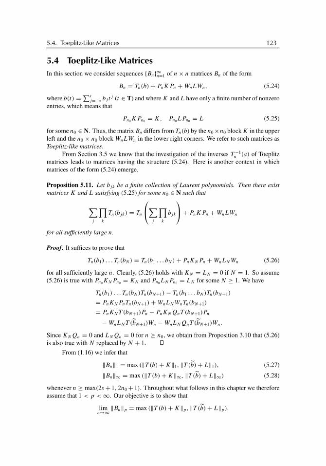
buch72005/10/5page 123

�

�

�

�

�

�

�

�

5.4. Toeplitz-Like Matrices 123

5.4 Toeplitz-Like MatricesIn this section we consider sequences {Bn}∞n=1 of n× n matrices Bn of the form

Bn = Tn(b)+ PnKPn +WnLWn, (5.24)

where b(t) =∑sj=−s bj t

j (t ∈ T) and where K and L have only a finite number of nonzeroentries, which means that

Pn0KPn0 = K, Pn0LPn0 = L (5.25)

for some n0 ∈ N. Thus, the matrix Bn differs from Tn(b) by the n0×n0 block K in the upperleft and the n0 × n0 block WnLWn in the lower right corners. We refer to such matrices asToeplitz-like matrices.

From Section 3.5 we know that the investigation of the inverses T −1n (a) of Toeplitz

matrices leads to matrices having the structure (5.24). Here is another context in whichmatrices of the form (5.24) emerge.

Proposition 5.11. Let bjk be a finite collection of Laurent polynomials. Then there existmatrices K and L satisfying (5.25) for some n0 ∈ N such that

∑j

∏k

Tn(bjk) = Tn

⎛⎝∑j

∏k

bjk

⎞⎠+ PnKPn +WnLWn


Proof. It suffices to prove that

Tn(b1) . . . Tn(bN) = Tn(b1 . . . bN)+ PnKNPn +WnLNWn (5.26)

for all sufficiently large n. Clearly, (5.26) holds with KN = LN = 0 if N = 1. So assume(5.26) is true with Pn0KNPn0 = KN and Pn0LNPn0 = LN for some N ≥ 1. We have

Tn(b1) . . . Tn(bN)Tn(bN+1)− Tn(b1 . . . bN)Tn(bN+1)

= PnKNPnTn(bN+1)+WnLNWnTn(bN+1)

= PnKNT (bN+1)Pn − PnKNQnT (bN+1)Pn

−WnLNT (bN+1)Wn −WnLNQnT (bN+1)Wn.

Since KNQn = 0 and LNQn = 0 for n ≥ n0, we obtain from Proposition 3.10 that (5.26)is also true with N replaced by N + 1.

From (1.16) we infer that

‖Bn‖1 = max (‖T (b)+K‖1, ‖T (b)+ L‖1), (5.27)

‖Bn‖∞ = max (‖T (b)+K‖∞, ‖T (b)+ L‖∞) (5.28)

whenever n ≥ max(2s+ 1, 2n0+ 1). Throughout what follows in this chapter we thereforeassume that 1 < p <∞. Our objective is to show that

limn→∞‖Bn‖p = max (‖T (b)+K‖p, ‖T (b)+ L‖p).

buch72005/10/5page 124

�

�

�

�

�

�

�

�


Since Wn → 0 weakly, we deduce from Proposition 3.3 that

WnLWn → 0 strongly, WnKWn → 0 strongly.

Consequently,

Bn → T (b)+K strongly, WnBnWn → T (b)+ L strongly.

Because ‖WnBnWn‖p = ‖Bn‖p, we deduce from Theorem 3.1 that

max (‖T (b)+K‖p, ‖T (b)+ L‖p) ≤ lim infn→∞ ‖Bn‖p. (5.29)

We define

Mp := max (‖T (b)+K‖p, ‖T (b)+ L‖p), M0p := ‖T (b)‖p. (5.30)

Lemma 5.12. We have ‖T (b)+K‖p ≥ ‖T (b)‖p and ‖T (b)+ L‖p ≥ ‖T (b)‖p.

Proof. For n ∈ Z, let χn(t) = tn (t ∈ T). From Proposition 1.4 we obtain the equalityT (χ−n)T (b)T (χn) = T (b). On the other hand, from (5.25) we see that KT (χn) = 0 for n ≥n0. Hence, for n ≥ n0, ‖T (b)‖p = ‖T (χ−n)(T (b)+K)T (χn)‖p, and since‖T (χ±n)‖p = 1,it follows that ‖T (b)‖p ≤ ‖T (b)+K‖p. Analogously we get ‖T (b)‖p ≤ ‖T (b)+L‖p. As‖T (b)‖p = limn→∞ ‖Tn(b)‖p and ‖T (b)‖p = limn→∞ ‖Tn(b)‖p, we deduce from Lemma5.3 that ‖T (b)‖p = ‖T (b)‖p. This gives the inequality ‖T (b)+ L‖p ≥ ‖T (b)‖p.

If s = 0, then

Bn = b0I + PnKPn +WnLWn,

and it is clear that

‖Bn‖p = max(‖b0I +K‖p, |b0|, ‖b0I + L‖p)

for n ≥ 2n0 + 1. As ‖b0I +K‖p ≥ |b0| and ‖b0I + L‖p ≥ |b0| by Lemma 5.12, it resultsthat

‖Bn‖p = max(‖b0I +K‖p, ‖b0I + L‖p) = Mp

for all n ≥ 2n0 + 1. Thus, in the following we will always assume that s ≥ 1. The desiredresult is Corollary 5.14. The next theorem gives the difficult part of that corollary and, inaddition, an upper estimate of ‖Bn‖p.

Theorem 5.13. If n ≥ max(8s + 8, 4n0), then

‖Bn‖p ≤ Mp

(1+ 8s

pn

).

Proof. Put � = [n/4] and let x = (xj )n−1j=0 ∈ �

pn be any vector such that ‖x‖p = 1. By

Lemma 5.4, there is an m ∈ N such that

�+ s ≤ m ≤ 3�− s,

m+s−1∑j=m−s

|xj |p ≤[�

s

]−1

. (5.31)

buch72005/10/5page 125

�

�

�

�

�

�

�

�

5.4. Toeplitz-Like Matrices 125

We now proceed as in the proof of Theorem 5.5. First, we have

‖Bnx‖pp =

m−1∑j=0

|(Bnx)j |p +n−1∑j=m

|(Bnx)j |p. (5.32)

It is clear that � ≤ n/4. By assumption, n ≥ 4n0, whence � = [n/4] ≥ n0. Thus,

n ≥ 4� = �+ 3� ≥ n0 + 3� > n0 + 3�− s ≥ n0 +m. (5.33)

If j ≤ m− 1, then (5.33) implies that

n− 1− j ≥ n−m > n0. (5.34)

Let K = (Kij ) and L = (Lij ). Since

(WnLWnx)j = (LWnx)n−1−j =n0−1∑i=0

Ln−1−j,ixn−1−i ,

we deduce from (5.25) and (5.34) that (WnLWnx)j = 0 whenever j ≤ m−1. Consequently,

m−1∑j=0

|(Bnx)j |p =m−1∑j=0

∣∣∣∣∣m+s−1∑

i=0

bj−ixi +n0−1∑i=0

Kjixi

∣∣∣∣∣p

= ‖Pm(T (b)+K)(xi)m+s−1i=0 ‖p

p

≤ ‖T (b)+K‖pp

m+s−1∑i=0

|xi |p ≤ Mpp

m+s−1∑i=0

|xi |p. (5.35)

Similarly, if j ≥ m then (PnKPnx)j = 0, whence

n−1∑j=m

|(Bnx)j |p =n−1∑j=m

∣∣∣∣∣n−1∑

i=m−s

bj−ixi +n0−1∑i=0

Ln−1−j,ixn−1−i

∣∣∣∣∣p

=n−1∑j=m

∣∣∣∣∣n−m+s−1∑

r=0

bj−n+1+rxn−1−r +n0−1∑r=0

Ln−1−j,rxn−1−r

∣∣∣∣∣p

=n−m−1∑

k=0

∣∣∣∣∣n−m+s−1∑

r=0

bn−1−k−n+1+rxn−1−r +n0−1∑r=0

Ln−1−n+1+k,rxn−1−r

∣∣∣∣∣p

=n−m−1∑

k=0

∣∣∣∣∣n−m+s−1∑

r=0

br−kxn−1−r +n0−1∑r=0

Lk,rxn−1−r

∣∣∣∣∣p

= ‖Pn−m(T (b)+ L)(xn−1−r )n−m+s−1r=0 ‖p

p

≤ ‖T (b)+ L‖pp

n−m+s−1∑r=0

|xn−1−r |p ≤ Mpp

n−1∑j=m−s

|xj |p. (5.36)

buch72005/10/5page 126

�

�

�

�

�

�

�

�


Combining (5.32), (5.35), and (5.36) we get

‖Bnx‖pp ≤ Mp

p

⎛⎝m+s−1∑j=0

|xj |p +n−1∑

j=m−s

|xj |p⎞⎠ ,

which, by (5.10), implies that ‖Bnx‖pp ≤ M

pp (1 + [�/s]−1). As [�/s] ≥ n/(8s) for n ≥

8+ 8s, it results that

‖Bn‖p ≤ Mp

(1+ 8s

n

)1/p

≤ Mp

(1+ 8s

pn

).

Corollary 5.14. We have

limn→∞‖Bn‖p = Mp.

Proof. The proof is immediate from (5.29), (5.30), and Theorem 5.13.

5.5 Exponentially Fast Convergence Is GenericWe now turn to the problem of estimating the speed with which ‖Bn‖p converges to Mp.The solution will be as follows: generically ‖Bn‖p converges to Mp exponentially fast, butin some exceptional cases it may happen that | ‖Bn‖p −Mp| decays only as 1/n2. Preciseresults are in this and the next sections.

Let Bn be as in the previous section and put m0 = max(s, n0) and B = T (b) + K .We know from Lemma 5.12 that always ‖B‖p ≥ ‖T (b)‖p.

The following lemma shows the existence of a rapidly decaying sequence at which B

attains its norm.

Lemma 5.15. If ‖B‖p > ‖T (b)‖p, then there exists an x0 = {x(0)j }∞j=0 ∈ �p such that

‖x0‖p = 1, ‖Bx0‖p = ‖B‖p, (5.37)

and ⎛⎝ ∞∑j=m

|x(0)j |p

⎞⎠1/p

≤(‖T (b)‖p

‖B‖p

)(m−(m0+s))/(2s)

(5.38)

for every m ≥ m0 + s.

Proof. Put M0 = ‖T (b)‖p and M = ‖B‖p. Pick any natural number m ≥ m0. There arexk = {x(k)

j }∞j=0 ∈ �p such that

‖xk‖p = 1, ‖Bxk‖p = Mp − δk, (5.39)

where δk goes monotonically to zero as k → ∞. As in the proof of Theorem 5.13 we seethat

Bxk = Pm(T (b)+K)(x(k)j )m+s−1

j=0 +QmT (b)(x(k)j )∞j=m−s ,

buch72005/10/5page 127

�

�

�

�

�

�

�

�

5.5. Exponentially Fast Convergence Is Generic 127

whence

Mp − δk ≤ Mp

m+s−1∑j=0

|x(k)j |p +M

p

0

∞∑j=m−s

|x(k)j |p. (5.40)

On defining

O(k)m =

∞∑j=m

|x(k)j |p, γk = δk/M

p, q = (M0/M)p,

we can rewrite (5.40) in the form 1− γk ≤ (1−O(k)m+s)+ qO

(k)m−s . Thus,

O(k)m+s ≤ qO

(k)m−s + γk for all m ≥ m0. (5.41)

Since O(k)m ≤ 1, we obtain from (5.41) that Om0+s+v ≤ q + γk for all v in the set

{0, 1, . . . , 2s − 1}. This and (5.41) give O(k)m0+3s+v ≤ qO

(k)m0+s+v + γk ≤ q2 + (q + 1)γk for

v ∈ {0, 1, . . . , 2s − 1}. Repeating this argument we arrive at the inequalities

Om0+(2j+1)s+v ≤ qj+1 + (qj + · · · + 1)γk ≤ qj+1 + γk

1− q(5.42)

for v ∈ {0, 1, . . . , 2s − 1}. Let r := q1/(2s). Then (5.42) can be written as

O(k)m0+s+2js+v ≤ qj+1 + γk

1− q= r2js+2s + γk

1− q,

and it results that

O(k)m0+s+� ≤ r� + γk

1− qfor � ≥ 0. (5.43)

We now show that {xk}∞k=1 can be taken to be a Cauchy sequence in �p. Given ε > 0,there is a natural number N such that r(N−(m0+s))/p < ε/4. On passing to a subsequenceif necessary, we can assume that {PNxk}∞k=1 is a Cauchy sequence in �

p

N . Hence, there is anatural number R such that

N−1∑j=0

|x(k1)j − x

(k2)j |p <

(ε

4

)p

,γk1 + γk2

1− q<

ε

4

whenever k1 ≥ R and k2 ≥ R. From (5.43) we now obtain that ‖xk1−xk2‖p does not exceed⎛⎝N−1∑j=0

|x(k1)j − x

(k2)j |p

⎞⎠1/p

+⎛⎝ ∞∑

j=N

|x(k1)j |p

⎞⎠1/p

+⎛⎝ ∞∑

j=N

|x(k2)j |p

⎞⎠1/p

≤ ε/4+(O

(k1)N

)1/p +(O

(k2)N

)1/p

≤ ε/4+ r(N−(m0+s))/p + r(N−(m0+s))/p + γk1 + γk2

1− q

< ε/4+ ε/4+ ε/4+ ε/4 = ε.

buch72005/10/5page 128

�

�

�

�

�

�

�

�


This shows that {xk} may be assumed to be a Cauchy sequence.Let x0 ∈ �p be the limit of xk as k → ∞. Passing to the limit k → ∞ in (5.39) we

arrive at (5.37). Repeating the above reasoning with xk replaced by x0 we get the analogueof (5.43) for x0, that is,

∞∑j=m0+s+�

|x(0)j |p ≤ r� for � ≥ 0. (5.44)

If m ≥ m0 + s, then m = m0 + s + � with � ≥ 0, and (5.44) reads

∞∑j=m

|x(0)j |p ≤ rm−(m0+s) =

(M0

M

)p(m−(m0+s))/(2s)

.

The following theorem exhibits a case in which ‖Bn‖p converges to Mp exponentiallyfast. Recall that m0 := max(s, n0).

Theorem 5.16. Suppose M0p < Mp. If n ≥ 4m0 + 4s + 2 then

Mp(1− cp�np) ≤ ‖Bn‖p ≤ Mp(1+ cp�n

p), (5.45)

where

cp = 2s

(Mp

M0p

)(2m0+4s+1)/(4s)

, �p =(

M0p

Mp

)1/(4s)

.

Proof. Put M0 = M0p and M = Mp. By Corollary 5.14, ‖Bn‖p → M . Hence there are

xn = (x(n)j )n−1

j=0 ∈ �pn such that

‖xn‖p = 1, ‖Bnxn‖p = ‖Bn‖p, ‖Bnxn‖pp = Mp

p + εn, (5.46)

where εn ∈ R and εn → 0 as n → ∞. Again set � = [n/4] and note that � > m0 byassumption. For � < m < 2�, we have

‖Bn‖pp =

m−1∑j=0

∣∣∣∣∣m+s−1∑

k=0

bj−kx(n)k +

n0−1∑k=0

Kjkx(n)k

∣∣∣∣∣p

+n−m−1∑j=m

∣∣∣∣∣n−m+s−1∑k=m−s

bj−kx(n)k

∣∣∣∣∣p

+n−1∑

j=n−m

∣∣∣∣∣n−1∑

k=n−m+s

bj−kx(n)k +

n0−1∑k=0

(WnLWn)jkx(n)k

∣∣∣∣∣p

≤ ‖(T (b)+K)(x(n)k )m+s−1

k=0 ‖pp + ‖T (b)(x

(n)k )n−m+s−1

k=m−s ‖pp

+ ‖(Tn(b)+WnLWn)(x(n)k )n−1

k=n−m+s‖pp.

Since Tn(b) = WnTn(b)Wn and ‖Wn‖p = 1, it follows from (5.46) that

Mp + εn ≤ Mp

m+s−1∑k=0

|x(n)k |p +M

p

0

n−m+s−1∑k=m−s

|x(n)k |p +Mp

n−1∑k=n−m+s

|x(n)k |p.

buch72005/10/5page 129

�

�

�

�

�

�

�

�

5.5. Exponentially Fast Convergence Is Generic 129

With

O(n)m :=

n−m−1∑j=m

|x(n)j |p,

we therefore get Mp+εn ≤ Mp(1−O(n)m+s)+M

p

0 O(n)m−s , whence O

(n)m+s ≤ qO

(n)m−s−γn with

q := (M0/M)p and γn := εn/Mp. This inequality is of the form (5.41). Consequently, in

analogy to (5.42) and (5.43) we have

O(n)m0+s+j ≤ rj − 1− rj

1− qγn, r := q1/(2s) (5.47)

as long as O(n)m0+s+j is well defined, i.e., for all j satisfying m0+s+j ≤ n−(m0+s+j)−1

or, equivalently, for

j ≤ n− 1

2−m0 − s = n− 2m0 − 2s − 1

2. (5.48)

As the left-hand side of (5.47) is nonnegative provided (5.48) holds, we get

γn ≤ (1− q)r(n−2m0−2s−1)/2

1− r(n−2m0−2s−1)/2≤ 1− q

1− rr(n−2m0−2s−1)/2

= 1− ((M0/M)p/(2s)

)2s

1− (M0/M)p/(2s)

(M0

M

) p

2s

n−2m0−2s−12

≤ 2s

(M0

M

) p

4s(n−2m0−2s−1)

≤ 2s

(M0

M

) 14s

(n−2m0−2s−1)

. (5.49)

Put ηn := ‖Bn‖p −M . By (5.46), ηn = (Mp + εn)1/p −M . If εn ≥ 0, then

ηn = M(

1+ εn

Mp

)1/p −M ≤ M

(+ εn

pMp

)−M = εn

pMp−1,

and if εn < 0, then ηn < 0. Since γn = εn/Mp, we see from (5.49) that in either case

ηn ≤ M

p2s

(M

M0

)(2m0+2s+1)/(4s) (M0

M

)n/(4s)

≤ Mcp�np.

This is the upper estimate in (5.45).To prove the lower estimate in (5.45) we make use of Lemma 5.15. For the sake of

definiteness, suppose M = ‖T (b) + K‖p (since ‖Bn‖p = ‖WnBnWn‖p, the case M =‖T (b)+L‖p can be reduced to the case we consider). Let x0 satisfy (5.37) and (5.38). Putv = [n/2] (> m0) and yn = Pvx0. Then ‖Bn‖p equals

‖Pn(T (b)+K)yn‖p = ‖(T (b)+K)yn −Qn(T (b)+K)yn‖p

= ‖(T (b)+K)(x(0)j )∞j=0 − (T (b)+K)(x

(0)j )∞j=v −Qn(T (b)+K)(x

(0)j )v−1

j=v−s‖p

buch72005/10/5page 130

�

�

�

�

�

�

�

�


and this is clearly greater than or equal to

‖(T (b)+K)x0‖p − ‖(T (b)+K)(x(0)j )∞j=v‖p − ‖Qn(T (b)+K)(x

(0)j )v−1

j=v−s‖p

≥ M − ‖(x(0)j )∞j=v‖p − ‖(x(0)

j )v−1j=v−s‖p ≥ M − 2M

⎛⎝ ∞∑j=v−s

|x(0)j |p

⎞⎠1/p

≥ M − 2M

(M0

M

)(v−s−(m0+s))/(2s)

≥ M − 2M

(M0

M

)((n−1)/2−s−(m0+s))/(2s)

,

which equals

M − 2M

(M

M0

)(2m0+4s+1)/(4s) (M0

M

)(n/(4s)

≥ M −Mcp�np.

Since ‖yn‖p ≤ 1, we finally obtain

‖Bn‖p ≥ ‖Bnyn‖p/‖yn‖p ≥ ‖Bnyn‖p ≥ M −Mcp�np.

The crucial assumption of Theorem 5.16 is the strict inequality M0p < Mp. In the case

p = 2, the following argument can be employed to see that this inequality is genericallytrue. Let P be the set of all Laurent polynomials and let X denote the set of all infinitematrices with only finitely many nonzero entries. We equip P × X × X with the norm‖(b, K, L)‖ := max(‖T (b)‖2, ‖K‖2, ‖L‖2). Recall that ‖T (b)‖2 = ‖b‖∞ (Theorem 1.15).

Proposition 5.17. The set

{(b, K, L) ∈ P × X × X : max(‖T (b)+K‖2, ‖T (b)+ L‖2) > ‖T (b)‖2} (5.50)

is an open and dense subset of P × X × X .

Proof. It is clear that (5.50) is an open subset of P × X × X . To show that it is dense inP×X ×X , it suffices to prove that the set of all (b, K) ∈ P×X satisfying ‖T (b)+K‖2 >

‖T (b)‖2 is dense in P × X . Pick (b, K) ∈ P × X and suppose

‖T (b)+K‖2 = ‖T (b)‖2 = ‖b‖∞.

Given any ε > 0, we can find a λ ∈ C such that |λ| < ε and ‖b + λ‖∞ > ‖b‖∞. Then

‖T (b)+K + λI‖2 = ‖T (b − λ)+K‖2 ≥ ‖T (b + λ)‖2 = ‖b + λ‖∞ > ‖b‖∞,

and since T (b)+K + λPn converges strongly to T (b)+K + λI , it follows that

lim infn→∞ ‖T (b)+K + λPn‖2 ≥ ‖T (b)+K + λI‖2 > ‖T (b)‖2.

Consequently, letting K0 := K + λPn, we see that ‖T (b) + K0‖2 > ‖T (b)‖2 for allsufficiently large n, while

‖(T (b)+K)− (T (b)+K0)‖2 ≤ |λ| ‖Pn‖2 = |λ| < ε.

Now let Bn be given by (5.24) and let p = 2. Proposition 5.17 tells us that the strictinequality M0

2 < M2 represents the generic case, whereas the equality M02 = M2 is the

exceptional case. Thus, Theorem 5.16 says that generically ‖Bn‖2−M2 decays to zero withexponential speed.

buch72005/10/5page 131

�

�

�

�

�

�

�

�

5.6. Slow Convergence 131

5.6 Slow ConvergenceIn concrete situations, we nevertheless often encounter the exceptional case where M0

p =Mp. For instance, we are definitely in this case whenever Bn = Tn(b). Theorem 5.8 revealsthat in the exceptional case it is possible that

M2 − ‖Bn‖2 = M02 − ‖Bn‖2 ≥ d/n2

with some d > 0 independent of n, which means that we do not have exponentially fastconvergence.

The following theorem certainly does not give sharp estimates, but it provides us witha universal estimate with good constants.

Theorem 5.18. If s ≥ 1 and n ≥ max(4n0, 81 s), then

M0p

(1− 81

p

s

n

)≤ ‖Bn‖p ≤ Mp

(1+ 8

p

s

n

).

Proof. The upper estimate is immediate from Theorem 5.13. So we are left to prove thelower estimate.

By Theorem 5.5, there is an x ∈ �p

[n/2] such that ‖x‖p = 1 and

‖T[n/2](b)x‖p ≥ M0p

(1− 40

p

s

[n/2])

.

Let � = [n/4] and define the unit vector y ∈ �pn by

y = (0, . . . , 0︸︷︷︸�

, x0, x1, . . . , x[n/2]−1, 0, . . . , 0︸︷︷︸�′

).

By assumption, � ≥ n0 and �′ ≥ n0. This implies that Bny = Tn(b)y, whence

‖Bny‖p = ‖Tn(b)y‖p ≥⎛⎝�+[n/2]∑

j=�+1

|(Tn(b)y)j |p⎞⎠1/p

=⎛⎝�+[n/2]∑

j=�+1

∣∣∣∣∣�+[n/2]∑k=�+1

bj−kxk

∣∣∣∣∣p⎞⎠1/p

= ‖T[n/2](b)x‖p

≥ M0p

(1− 40

p

s

[n/2])≥ M0

p

(1− 40

p

2s

n− 1

)≥ M0

p

(1− 81

p

s

n

),

the last estimate resulting from the assumption that n ≥ 81s ≥ 81.

Corollary 5.19. Suppose M0p = Mp. If s ≥ 1 and n ≥ max(4n0, 81 s), then

Mp

(1− 81

p

s

n

)≤ ‖Bn‖p ≤ Mp

(1+ 8

p

s

n

).

Proof. The proof is immediate from Theorem 5.18.

buch72005/10/5page 132

�

�

�

�

�

�

�

�


5.7 SummaryLet us summarize the essence of this chapter. We are given matrices

Bn = Tn(b)+ PnKPn +WnLWn,

where b is a Laurent polynomial and K and L have only finitely many nonzero entries. Weput

Mp := max (‖T (b)+K‖p, ‖T (b)+ L‖p), M0p := ‖T (b)‖p.

The inequality Mp ≥ M0p is always true, and we know that at least for p = 2 the strict

inequality Mp > M0p represents the generic case.

If 1 M0p, then there is a γ > 0 such that∣∣∣ ‖Bn‖p −Mp

∣∣∣ = O(e−γ n), (5.51)

while if 1 < p <∞ and Mp = M0p, then

∣∣∣ ‖Bn‖p −Mp

∣∣∣ = O

(1

n

). (5.52)

If p = 1 or p = ∞, then ∣∣∣ ‖Bn‖p −Mp

∣∣∣ = 0 (5.53)

for all sufficiently large n.Now suppose that Bn = Tn(b) is a pure Toeplitz band matrix. In this case, Mp =

M0p = ‖T (b)‖p. If 1 < p <∞, then

∣∣∣ ‖Tn(b)‖p − ‖T (b)‖p

∣∣∣ = O

(1

n

). (5.54)

In the case p = 2 this can be improved to∣∣∣ ‖Tn(b)‖2 − ‖T (b)‖2

∣∣∣ = O

(1

n2

). (5.55)

The convergence in (5.55) may be faster, of the form O(1/n2γ ) with some natural numberγ , but it is never exponentially fast unless |b| is constant on T (which happens if and onlyif b has at most one nonzero coefficient). Finally, if p = 1 or p = ∞, then∣∣∣ ‖Tn(b)‖p − ‖T (b)‖p

∣∣∣ = 0 (5.56)

for all n large enough.

buch72005/10/5page 133

�

�

�

�

�

�

�

�

Exercises 133

Exercises

1. Let A ∈ B(�2) be selfadjoint and positive definite. Put An = PnAPn. Prove that{An}∞n=1 is a stable sequence and that

‖An‖2 ≤ ‖A‖2 for all n ≥ 1, limn→∞‖An‖2 = ‖A‖2,

‖A−1n ‖2 ≤ ‖A−1‖2 for all n ≥ 1, lim

n→∞‖A−1n ‖2 = ‖A−1‖2.

2. Let b ∈ P and let Pcirc(Tn(b)) be the circulant matrix whose first column is

col

((n− j)bj + jb−(n−j)

n

)n−1

j=0

(with b−n := 0).

Prove that Pcirc(Tn(b)) is the best approximation of Tn(b) by a circulant matrix in theFrobenius norm.

3. Let a, b ∈ P . Prove that

‖Tn(a)Tn(b)− Tn(b)Tn(a)‖p = ‖T (a)T (b)− T (b)T (a)‖p


4. Let α and β be positive integers and put

An =

⎛⎜⎜⎜⎜⎜⎝0 1α 2α . . . (n− 1)α

1β 0 1α . . . (n− 2)α

2β 1β 0 . . . (n− 3)α

......

.... . .

...

(n− 1)β (n− 2)β (n− 3)β . . . 0

⎞⎟⎟⎟⎟⎟⎠ .

Prove that ‖An‖2F/(n‖An‖2

2)→ 0 as n→∞, where ‖ · ‖F is the Frobenius norm.

5. Consider the sequence {212, 222

, 232, 242

, 252, . . . }. Define ak = k if k belongs to this

sequence and ak = 0 otherwise. Let An be the lower-triangular Toeplitz matrix

An =

⎛⎜⎜⎜⎝a0

a1 a0...

.... . .

an−1 an−2 . . . a0

⎞⎟⎟⎟⎠ .

Prove that for each number μ in the segment [0, 1] there exists a sequence {nj }∞j=1

such that ‖Anj‖2

F/(nj‖Anj‖2

2)→ μ as nj →∞.

6. Let a be a complex number with |a| ≥ 4. Let b(t) = 2+ t + t−1 and put

Bn = Tn(b)+ diag (a, 0, . . . , 0, a), B = T (b)+ diag (a, 0, . . . ).

buch72005/10/5page 134

�

�

�

�

�

�

�

�


Show that for n ≥ 10,

∣∣∣ ‖Bn‖2 − ‖B‖2

∣∣∣ <1

5(|a| + 2)

114

(4√|a|2 + 1

) n4

.

7. Let

B = T (b)+K =

⎛⎜⎜⎝3 84 0 . . .

−1 3 −1 . . .

0 −1 3 . . .

. . . . . . . . . . . .

⎞⎟⎟⎠and Bn = Tn(b)+ PnKPn.

(a) Show that M02 = 5 and 80 ≤ M2 ≤ 90.

(b) Use Theorem 5.16 to show that for n ≥ 14,∣∣∣ ‖Bn‖2 − ‖B‖2

∣∣∣ <120150

2n.

(c) MATLAB gives ‖B32‖2 = 84.1117. Deduce that

‖B‖2 = 84.1117± 0.0001.

8. Show that if ϕ ∈ L∞ and

T2(ϕ) =(

0 11 0

),

then ‖ϕ‖∞ ≥√

2.

Notes

Section 5.1 is from [58]. The results of Section 5.2 are well known in the case where b isreal valued and, hence, Tn(b) is Hermitian: See Kac, Murdock, and Szegö [176], Grenanderand Szegö [145], Widom [290], Parter [198], and Serra Capizzano [247], [248]. In the formstated here, Theorem 5.8 was established in [58].

Theorem 5.10 probably first appears in our paper [53]. Our original proof of Theorem5.10 used the Fejér kernel and gave only the inequality

‖Tn(b)‖2 ≥ (1/√

3π) ‖σnb‖∞,

which, however, was sufficient for the purpose of our paper [53]. Then Stefano Serra Capiz-zano communicated an alternative proof to us which, moreover, showed that the constant1/√

3π can be improved to the (optimal) value 1. Subsequently we were able to modify(and even to simplify) our original proof so that it yielded the constant 1 as well, but thiswas no longer the point. Serra Capizzano’s proof was based on arguments that are stan-dard in the preconditioning literature (see, e.g., [84], [88], [249]). He first showed that

buch72005/10/5page 135

�

�

�

�

�

�

�

�

Notes 135

‖Tn(b)‖2 ≥ ‖Pcirc(Tn(b))‖2, where Pcirc(Tn(b)) is the circulant matrix of Exercise 2. Onecan straightforwardly verify that

‖Pcirc(Tn(b))‖2 = maxt∈Tn

|(σnb)(t)|, (5.57)

where Tn is the group of the nth unit roots. A scaling trick, viz., the equality ‖Tn(b)‖2 =‖Tn(bζ )‖2 with (bζ )j := bj ζ

j (ζ ∈ T), eventually gives the desired inequality

‖Tn(b)‖2 = maxζ∈T

‖Tn(bζ )‖2 ≥ maxζ∈T

maxt∈Tn

|(σnbζ )(t)|= max

ζ∈Tmaxt∈Tn

|(σnb)(ζ t)| = ‖σnb‖∞.

In an attempt to find out who was the first to write down (5.57) explicitly, we looked into thepaper [249], and once we saw the first lines of the proof of Lemma 2.1 of [249], we cameto understand that our Theorem 5.10 can actually be proved as in Section 5.3.

The results of Sections 5.4 to 5.7 are also taken from paper [58].Figure 5.1 was done by André Eppler. For Exercises 4 and 5 see [53]. Exercise 8 is

from [194], where it is attributed to A. Volberg.

Further results: symbols of minimal norm. Suppose we are given a Toeplitz matrixTn(a). Since only the Fourier coefficients ak with |k| ≤ n − 1 enter the matrix, we haveTn(a) = Tn(ϕ) for every ϕ ∈ L∞ satisfying ϕk = ak for |k| ≤ n− 1. Put

νn(a) = inf{‖ϕ‖∞ : ϕk = ak for |k| ≤ n− 1}.

It is clear that ‖Tn(a)‖2 ≤ νn(a) ≤ ‖a‖∞. Nikolskaya and Farforovskaya [194] showedthat actually

‖Tn(a)‖2 ≥ 1

3νn(a).

Thus, we can find a symbol ϕ ∈ L∞ such that

Tn(a) = Tn(ϕ) and ‖Tn(a)‖2 ≤ ‖ϕ‖∞ ≤ 3‖Tn(a)‖2.

From Exercise 8 we learn that if a(t) = t + t−1, then ν2(a) ≥ √2, which implies that

1 = ‖T2(a)‖2 ≥ c ν2(a) ≥ c√

2

cannot be true if c > 1/√

2. We so arrive at the conclusion that the optimal constant in theinequality ‖Tn(a)‖2 ≥ c νn(a) is in [1/3, 1/

√2].

Together with Tn(a) = PnT (a)Pn we may also consider the rectangular Toeplitzmatrices

Tn−r,n+r (a) = Pn−rT (a)Pn+r (|r| ≤ n− 1).

buch72005/10/5page 136

�

�

�

�

�

�

�

�


For example, in the case n = 3 we have the five matrices

T5,1(a) =

⎛⎜⎜⎜⎜⎝a−2

a−1

a0

a1

a2

⎞⎟⎟⎟⎟⎠ , T4,2(a) =

⎛⎜⎜⎝a−1 a−2

a0 a−1

a1 a0

a2 a1

⎞⎟⎟⎠ ,

T3,3(a) =⎛⎝ a0 a−1 a−2

a1 a0 a−1

a2 a1 a0

⎞⎠ , T2,4(a) =(

a1 a0 a−1 a−2

a2 a1 a0 a−1

),

T1,5(a) = (a2 a1 a0 a−1 a−2

).

Put

δn(a) = max|r|≤n−1‖Tn−r,n+r (a)‖2.

Again it is obvious that δn(a) ≤ νn(a) ≤ ‖a‖∞. Bakonyi and Timotin [12] proved theestimate

δn(a) ≥ 1

2

n+ 2

n+ 1νn(a).

Consequently, there is a symbol ϕ ∈ L∞ such that

Tn(a) = Tn(ϕ) and δn(a) ≤ ‖ϕ‖∞ ≤ 2n+ 1

n+ 2δn(a).

buch72005/10/5page 137

�

�

�

�

�

�

�

�

Chapter 6

ConditionNumbers

Let Bn be an n× n matrix. For 1 ≤ p ≤ ∞, we denote by κp(Bn) the condition number ofBn as an operator on �

pn :

κp(Bn) := ‖Bn‖p ‖B−1n ‖p.

Throughout what follows we put ‖B−1n ‖p = ∞ in case Bn is not invertible.

In this chapter, we study the behavior of the condition numbers of Toeplitz bandmatrices Tn(b) and of Toeplitz-like matrices Bn = Tn(b)+ PnKPn +WnLWn for large n.

6.1 Asymptotic Inverses of Toeplitz-Like MatricesAs in Section 5.4, we assume that Bn is given by

Bn = Tn(b)+ PnKPn +WnLWn, (6.1)

where b(t) =∑sj=−s bj t

j (t ∈ T) and where K and L have only a finite number of nonzeroentries, that is,

Pn0KPn0 = K, Pn0LPn0 = L (6.2)

for some n0 ∈ N. Theorem 3.15 gives an asymptotic inverse for the pure Toeplitz matricesTn(b). The purpose of this section is to extend this result to the Toeplitz-like matrices Bn.

We put

B = T (b)+K, B = T (b)+ L, (6.3)

and in case B and B are invertible (which, by Theorem 1.9, implies that b is invertible andthat wind b = 0), we set

X = B−1 − T (b−1), Y = B−1 − T (b−1). (6.4)

137

buch72005/10/5page 138

�

�

�

�

�

�

�

�

138 Chapter 6. Condition Numbers

Lemma 6.1. Let 1 ≤ p ≤ ∞ and let α be any number satisfying (1.23). If B and B areinvertible on �p, then ‖QnX‖p = O(e−αn) and ‖QnY‖p = O(e−αn) as n→∞.

Proof. From (6.4) we infer that I = (T (b−1) + X)(T (b) + K). This and Proposition 1.3yield

I = X(T (b)+K)+ T (b−1)T (b)+ T (b−1)K

= X(T (b)+K)+ I −H(b−1)H (b)+ T (b−1)K,

whence X = (H(b−1)H (b)− T (b−1)K)(T (b)+K)−1 and thus

‖QnX‖p ≤(‖QnH(b−1)‖p ‖H(b)‖p + ‖QnT (b−1)K‖p

)‖(T (b)+K)−1‖p.

Taking into account that K has only a finite number of nonzero entries and using Lemma1.17 it is easy to show that ‖QnH(b−1)‖p and ‖QnT (b−1)K‖p are O(e−αn), which impliesthat ‖QnX‖p = O(e−αn). The proof is analogous for ‖QnY‖p.

Theorem 6.2. Let 1 ≤ p ≤ ∞, let α satisfy (1.23), and suppose B and B are invertible on�p. Then the matrices Bn are invertible for all sufficiently large n and

B−1n = Tn(b

−1)+ PnXPn +WnYWn + En,

where X and Y are given by (6.4) and ‖En‖p = O(e−αn).

Proof. Put An = Tn(b−1)+ PnXPn +WnYWn. Theorem 3.13 tells us that the matrices Bn

are invertible for all sufficiently large n and that ‖B−1n ‖p remains bounded as n →∞. We

have En = B−1n −An = B−1

n (Pn −BnAn), and the theorem will follow as soon as we haveshown that ‖Pn − BnAn‖p = O(e−αn). The matrix BnAn − Pn equals

Pn(T (b)+K)Pn(T (b−1)+X)Pn − Pn

+ Pn(T (b)+K)PnWnYWn +WnLWnPn(T (b−1)+X)Pn +WnLWnWnYWn.

Let n0 be the number in (6.2). Since Pn0Wn = Wn0T (χ−(n−n0))PnQn−n0 for all n ≥ n0, weobtain from (6.2) that

PnKPnWnYWn = Pn0KPn0WnYWn = Pn0KWn0T (χ−(n−n0))PnQn−n0YWn,

and Lemma 6.1 therefore gives ‖PnKPnWnYWn‖p = O(e−αn). Analogously one can showthat ‖WnLWnPnXPn‖ = O(e−αn). Thus BnAn − Pn is


+ PnT (b)PnWnYWn +WnLWnPnT (b−1)Pn +WnLWnWnYWn + E′n (6.5)

with ‖E′n‖p = O(e−αn). The identities

PnT (b)WnYWn = WnT (b)PnYWn,

WnLWnT (b−1)Pn = WnLPnT (b−1)Wn,

buch72005/10/5page 139

�

�

�

�

�

�

�

�

6.2. The Limit of the Condition Numbers 139

imply that (6.5) equals


+Wn(T (b)+ L)Pn(T (b−1)+ Y )Wn −WnT (b)PnT (b−1)Wn + E′n, (6.6)

and since (T (b)+K)(T (b−1)+ X) = (T (b)+ L)(T (b−1)+ Y ) = I , it results that (6.6)is equal to

Pn − Pn(T (b)+K)Qn(T (b−1)+X)Pn − Pn

+ Pn −Wn(T (b)+ L)Qn(T (b−1)+ Y )Wn −WnT (b)PnT (b−1)Wn + E′n. (6.7)

Using (6.2) and Lemma 6.1 we see that (6.7) is

Pn − PnT (b)QnT (b−1)Pn − Pn

+ Pn −WnT (b)QnT (b−1)Wn −WnT (b)PnT (b−1)Wn + E′′n (6.8)

with ‖E′′n‖p = O(e−αn). Finally, taking into account Propositions 1.3 and 3.10 we obtain

that (6.8) minus E′′n is

Pn − PnT (b)QnT (b−1)Pn −WnT (b)T (b−1)Wn

= Pn − PnT (b)T (b−1)Pn + PnT (b)PnT (b−1)Pn −WnT (b)T (b−1)Wn

= Pn − Pn(I −H(b)H (b−1))Pn + Tn(b)Tn(b−1)−Wn(I −H(b)H(b−1))Wn

= Pn − Pn + PnH(b)H (b−1)Pn + Tn(b)Tn(b−1)− Pn +WnH(b)H(b−1)Wn

= Pn − Pn + Pn − Pn = 0.

Thus, BnAn − Pn = E′′n .

6.2 The Limit of the Condition NumbersLet Bn be of the form (6.1) and define B and B by (6.3). We know from Theorem 3.13 that‖B−1

n ‖p →∞ if B or B is not invertible. So suppose B and B are invertible and put

Np := max(‖B−1‖p, ‖B−1‖p).

Again by Theorem 3.13, the matrices Bn are invertible for all sufficiently large n andlim sup ‖B−1

n ‖p < ∞. The following theorem shows that in fact the limit lim ‖B−1n ‖p

exists and it identifies this limit.

Theorem 6.3. If 1 ≤ p ≤ ∞, then

limn→∞‖B

−1n ‖p = Np. (6.9)

Proof. Fix ε > 0. By virtue of Theorem 6.2,

B−1n = Tn(b

−1)+ PnXPn +WnYWn + En,

buch72005/10/5page 140

�

�

�

�

�

�

�

�


where X and Y are given by (6.4) and ‖En‖p = O(e−αn). We can choose a Laurentpolynomial a such that ‖b − a−1‖W < ε and ‖b−1 − a‖W < ε. Due to Lemma 6.1, thereexist infinite matrices U and V with only finitely many entries such that ‖X−U‖p < ε and‖Y − V ‖p < ε. Put

An = Tn(a)+ PnUPn +WnV Wn, Mp = max(‖T (a)+ U‖p, ‖T (a)+ V ‖p).

Corollary 5.14 implies that ∣∣ ‖An‖p −Mp

∣∣ < ε (6.10)

for all sufficiently large n. We have∣∣ ‖B−1n ‖p − ‖An‖p

∣∣= ∣∣ ‖Tn(b

−1)+ PnXPn +WnYWn + En‖p − ‖Tn(a)+ PnUPn +WnV Wn‖p

∣∣≤ ‖Tn(b

−1 − a)‖p + ‖Pn(X − U)Pn‖p + ‖Wn(Y − V )Wn‖p + ‖En‖p

≤ ‖b−1 − a‖W + ‖X − U‖p + ‖Y − V ‖p + ‖En‖p < 4ε (6.11)

provided n is large enough. Furthermore,

|Mp −Np |= ∣∣ max(‖T (a)+ U‖p, ‖T (a)+ V ‖p)−max(‖B−1‖p, ‖B−1‖p)

∣∣≤ max

(| ‖T (a)+ U‖p − ‖B−1‖p |, | ‖T (a)+ V ‖p − ‖B−1‖p |)

≤ max(‖T (a)+ U − B−1‖p , ‖T (a)+ V − B−1‖p

)= max

(‖T (a − b−1)+ U −X‖p , ‖T (a − b−1)+ V − Y‖p

)≤ max

(‖a − b−1‖W + ‖U −X‖p, ‖a − b−1‖W + ‖V − Y‖p

)< max (ε + ε, ε + ε) = 2ε. (6.12)

Putting (6.10), (6.11), (6.12) together, we arrive at the conclusion that

| ‖B−1n ‖p −Np | < ε + 4ε + 2ε = 7ε


Corollary 6.4. Let 1 ≤ p ≤ ∞. If B �= 0 or B �= 0, then

limn→∞ κp(Bn) = MpNp, (6.13)

where Mp = max(‖B‖p, ‖B‖p) and Np = max(‖B−1‖p, ‖B−1‖p).

Proof. This is immediate from Corollary 5.14 and Theorem 6.3. (Notice that if B = B = 0,then the assertion reads lim 0 = 0 · ∞.)

Corollary 6.5. If 1 ≤ p ≤ ∞ and b is a Laurent polynomial that does not vanish identically,then

limn→∞‖T

−1n (b)‖p = max(‖T −1(b)‖p, ‖T −1(b)‖p), (6.14)

limn→∞ κp(Tn(b)) = max(κp(T (b)), κp(T (b))). (6.15)

buch72005/10/5page 141

�

�

�

�

�

�

�

�

6.2. The Limit of the Condition Numbers 141

Proof. In the case where T (b) is invertible, formula (6.14) is a special case of Theorem 6.3and formula (6.15) follows from Corollary 6.4:

limn→∞‖Tn(b)‖p‖T −1

n (b)‖p = ‖T (b)‖p limn→∞‖T

−1n (b)‖p

= ‖T (b)‖p max(‖T −1(b)‖p, ‖T −1(b)‖p)

= max(‖T (b)‖p‖T −1(b)‖p, ‖T (b)‖p‖T −1(b)‖p)

= max(‖T (b)‖p‖T −1(b)‖p, ‖T (b)‖p‖T −1(b)‖p),

the equality ‖T (b)‖p = ‖T (b)‖p resulting from Theorem 1.14 for p = 1 and p = ∞ andfrom Lemma 5.3 for 1 < p < ∞. If T (b) is not invertible, then Theorem 3.7 tells us thatboth sides of (6.14) and (6.15) are infinite.

If p = 2, then ‖T (b)‖2 = ‖T (b)‖2 = ‖b‖∞ and ‖T −1(b)‖2 = ‖T −1(b)‖2 (note thatT (b) is just the transpose of T (b)), whence

limn→∞‖T

−1n (b)‖2 = ‖T −1(b)‖2, lim

n→∞ κ2(Tn(b)) = κ2(T (b)). (6.16)

As the following example shows, the situation is different for p �= 2.

Example 6.6. Let

a(t) = 1

a−(t)a+(t), a−(t) = 4+ 4t−1 + 3t−2, a+(t) = 2− t.

It is easily seen that a± ∈ GW± (Theorem 1.7). Thus, T (a) is invertible and T −1(a) =T (a+)T (a−) due to Proposition 1.4. We have

T (a+)T (a−) =

⎛⎜⎜⎝2 0 0 . . .

−1 2 0 . . .

0 −1 2 . . .

. . . . . . . . . . . .

⎞⎟⎟⎠⎛⎜⎜⎝

4 4 3 0 . . .

0 4 4 3 . . .

0 0 4 4 . . .

. . . . . . . . . . . . . . .

⎞⎟⎟⎠

=

⎛⎜⎜⎝8 8 6 0 0 . . .

−4 4 5 6 0 . . .

0 −4 4 5 6 . . .

. . . . . . . . . . . . . . . . . .

⎞⎟⎟⎠ .

This in conjunction with (1.16) shows that

‖T −1(a)‖1 = max(12, 16, 19) = 19, ‖T −1(a)‖1 = max(22, 19) = 22.

Since ‖T (a)‖1 = ‖T (a)‖1 = ‖a‖W , it follows that

‖T −1(a)‖1 < ‖T −1(a)‖1, κ1(T (a)) < κ1(T (a)).

If ‖bn − a‖W → 0, then

‖T −1(bn)− T −1(a)‖1 ≤ ‖T −1(a)‖1 ‖a − bn‖W ‖T −1(bn)‖1 → 0,

buch72005/10/5page 142

�

�

�

�

�

�

�

�


and hence we can find a Laurent polynomial b such that

‖T −1(b)‖1 < ‖T −1(b)‖1, κ1(T (b)) < κ1(T (b)).

By the Riesz-Thorin interpolation theorem, the numbers

log ‖T −1(b)‖p, log ‖T −1(b)‖p, log ‖T (b)‖p, log ‖T (b)‖p

are convex functions of 1/p ∈ [0, 1]. These functions are therefore continuous, whichimplies that if p > 1 is sufficiently close to 1, then

‖T −1(b)‖p < ‖T −1(b)‖p, κp(T (b)) < κp(T (b)).

The moral is that, in general, we cannot remove the maxima in formulas (6.14) and (6.15)for p �= 2.

6.3 Convergence Speed EstimatesAgain let Bn = Tn(b) + PnKPn + WnLWn be as in Section 6.1, set B = T (b) + K ,B = T (b)+ L, and put

Np = max(‖B−1‖p, ‖B−1‖p), N0p = ‖T (b−1)‖p.

Theorem 6.7. Let 1 N0

p, then there is a γ > 0 depending only on b, K, L such that∣∣ ‖Bn‖p −Np

∣∣ = O(e−γ√

n). (6.17)

If Np = N0p, then

∣∣ ‖Bn‖p −Np

∣∣ = O

(log n

n

). (6.18)

Proof. We know from Theorem 6.2 that B−1n = Tn(a) + PnXPn +WnYWn + En, where

a = b−1, X and Y are given by (6.4), and ‖En‖p = O(e−αn). Let s(n) be a sequence ofnatural numbers such that

s(n)→∞,n

s(n)→∞. (6.19)

Put Xs(n) = Ps(n)XPs(n), Ys(n) = Ps(n)YPs(n), and let cn denote the s(n)th partial sum of theFourier series of a. Set

An = Tn(cn)+ PnXs(n)Pn +WnYs(n)Wn. (6.20)


‖a − cn‖W = O(�s(n)) with some � < 1. (6.21)

buch72005/10/5page 143

�

�

�

�

�

�

�

�

6.3. Convergence Speed Estimates 143

We have∣∣ ‖B−1n ‖p − ‖An‖p

∣∣ ≤ ‖B−1n − An‖p

≤ ‖Tn(a − cn)‖p + ‖Pn(X −Xs(n))Pn‖p + ‖Wn(Y − Ys(n))Wn‖p + ‖En‖p

≤ ‖a − cs(n)‖W + ‖X −Xs(n)‖p + ‖Y − Ys(n)‖p + ‖En‖p. (6.22)

By Lemma 6.1, ‖X− PsXPs‖p = O(σ s) and ‖Y − PsYPs‖p = O(σ s) with σ = e−α < 1as s →∞. This and (6.17) show that (6.22) is

O(�s(n))+O(σ s(n))+O(σ s(n))+O(σ s(n)) = O(τ s(n)),

where max(�, σ ) < τ < 1. Let

Mp(s(n)) = max(‖T (cn)+Xs(n)‖p, ‖T (cn)+ Ys(n)‖p), M0p(s(n)) = ‖T (cn)‖p.

Then |Mp(s(n))−Np | does not exceed

max(∣∣ ‖T (cn)+Xs(n)‖p − ‖T (a)+X‖p

∣∣ , ∣∣ ‖T (cn)+ Ys(n)‖p − ‖T (a)+ Y‖p

∣∣)≤ max

(‖T (cn − a)+Xs(n) −X‖p, ‖T (cn − a)+ Ys(n) − Y‖p

),

and again taking into account (6.21) and Lemma 6.1 we see that this is

O(�s(n))+O(σ s(n)) = O(τ s(n)).

Furthermore, also by (6.21),∣∣M0p(s(n))−N0

p

∣∣= ∣∣ ‖T (cn)‖p − ‖T (a)‖p

∣∣ ≤ ‖T (cn − a)‖p = O(�s(n)) = O(τ s(n)).

In summary, at the present moment we have shown that∣∣ ‖B−1n ‖p −Np

∣∣ ≤ ∣∣ ‖An‖p −Mp(s(n))∣∣+O(τ s(n)) (6.23)

and that

Mp(s(n)) = Np +O(τ s(n)), M0p(s(n)) = N0

p +O(τ s(n)). (6.24)

Now suppose that Np > N0p. Then, by (6.24), Mp(s(n)) > M0

p(s(n)) for all suffi-ciently large n, and Theorem 5.16 therefore gives∣∣ ‖An‖p −Mp(s(n))

∣∣≤ 2s(n)Mp(s(n))

(Mp(s(n))

M0p(s(n))

)(6s(n)+1)/(4s(n)) (M0

p(s(n))

Mp(s(n))

)n/(4s(n))

≤ 2s(n)Mp(s(n))

(Mp(s(n))

M0p(s(n))

)2 (M0

p(s(n))

Mp(s(n))

)n/(4s(n))

. (6.25)

buch72005/10/5page 144

�

�

�

�

�

�

�

�


Choose any ε > 0 so that (N0p + ε)/(Np − ε) ∈ (0, 1) and assume that τ ∈ (0, 1) is larger

than (N0p + ε)/(Np − ε). If n is sufficiently large, then (6.25) is at most

2s(n)(Np + ε)

(Np + ε

N0p − ε

)2 (N0

p + ε

Np − ε

)n/(4s(n))

= O(s(n)τn/(4s(n))

).

This in conjunction with (6.23) yields the estimate∣∣ ‖B−1n ‖p −Np

∣∣ = O(s(n)τn/(4s(n))

).

Letting s(n) = [√n ], we obtain (6.17) with any γ > 0 such that τ 1/4 < e−γ .Now assume Np = N0

p. Then Mp(s(n)) ≥ M0p(s(n)) for all n by virtue of Lemma

6.10. From Theorem 5.13 and (6.24) we obtain

‖An‖p −Mp(s(n)) ≤ 8

pMp(s(n))

s(n)

n= O

(s(n)

n

),

while the lower estimate of Theorem 5.18 and (6.24) give

−‖An‖p +Mp(s(n))

≤ 81

pM0

p(s(n))s(n)

n+ ∣∣Mp(s(n))−M0

p(s(n))∣∣

= O

(s(n)

n

)+O(τ s(n))

(to get the O(τ s(n)) we used (6.24) and the equality Np = N0p). Choose γ > 0 and α > 0

so that τ < e−γ and γα > 1. Then put s(n) = [α log n]. Clearly, (6.19) is satisfied. As

O

(s(n)

n

)= O

(log n

n

),

O(τ s(n)) = O(e−γα log n) = O(n−γα) = O

(log n

n

),

we get (6.18) from (6.23).

Theorem 6.8. Let p = 1 or p = ∞ and suppose B and B are invertible. Let further α > 0be any number satisfying (1.23). Then∣∣ ‖Bn‖p −Np

∣∣ = O(e−αn/2). (6.26)

Proof. Write B−1n as in the proof of Theorem 6.7, put s(n) = [n/2] − 1, and define An by

(6.20). Proceeding in the way we derived (6.22) and using Lemmas 1.17 and 6.1, we get∣∣ ‖B−1n ‖p − ‖An‖p

∣∣≤ ‖a − cn‖W + ‖X −Xs(n)‖p + ‖Y − Ys(n)‖p + ‖En‖p

= O(e−αs(n)) = O(e−αn/2). (6.27)

buch72005/10/5page 145

�

�

�

�

�

�

�

�

6.4. Generic and Exceptional Cases 145

Since 2s(n)+ 1 ≤ n, we may employ (5.27) and (5.28) to conclude that

‖An‖p = max(‖T (cn)+Xs(n)‖p, ‖T (cn)+ Ys(n)‖p

),

whence, again by Lemmas 1.17 and 6.1,∣∣ ‖An‖p −Np

∣∣≤ max

(‖cn − a‖W + ‖X −Xs(n)‖p, ‖cn − a‖W + ‖Y − Ys(n)‖p

)= O(e−αs(n)) = O(e−αn/2). (6.28)

Combining (6.27) and (6.28) we arrive at the asserted estimate (6.26).

Recall that

Mp = max(‖B‖p, ‖B‖p), M0p = ‖T (b)‖p (6.29)

Np = max(‖B−1‖p, ‖B−1‖p), N0p = ‖T (b−1)‖p. (6.30)

Theorem 6.9. Suppose B and B are invertible on �p.If 1 M0

p, and Np > N0p, then there is a constant γ > 0 (depending

on p, b, K, L) such that ∣∣ κp(Bn)−MpNp

∣∣ = O(e−γ√

n). (6.31)

If 1 0 satisfies (1.23).

Proof. Estimate (6.31) follows from (5.51) and Theorem 6.7, estimate (6.32) is a conse-quence of (5.51), (5.52), and Theorem 6.7, and equality (6.33) results from (5.27), (5.28),and Theorem 6.8.

6.4 Generic and Exceptional Cases

Let Bn = Tn(b)+PnKPn+WnLWn be as in Section 6.1, put B = T (b)+K , B = T (b)+L,and define Mp, M0

p, Np, N0p by (6.29) and (6.30).

Lemma 6.10. Let 1 ≤ p ≤ ∞. We always have M0p ≤ Mp and N0

p ≤ Np.

Proof. The inequality M0p ≤ Mp follows from Lemma 5.12 for 1 < p <∞ and from

(1.16) for p = 1 and p = ∞. To prove that N0p ≤ Np, note first that B−1 = T (b−1) + X

buch72005/10/5page 146

�

�

�

�

�

�

�

�


by (6.4). Hence QnB−1Qn = QnT (b−1)Qn + QnXQn, and since ‖QnT (b−1)Qn‖p =

‖T (b−1)‖p and ‖QnXQn‖p → 0 (Lemma 6.1), it follows that lim ‖QnB−1Qn‖p =

‖T (b−1)‖p. As ‖B−1‖p ≥ ‖QnB−1Qn‖p, we conclude that ‖B−1‖p ≥ ‖T (b−1)‖p. Anal-

ogously, ‖B−1‖p ≥ ‖T (b−1)‖p = ‖T (b−1)‖p.

In Chapter 5, we observed that the norm ‖Bn‖p converges exponentially fast to Mp ifMp > M0

p, while the convergence may be slow in the case Mp = M0p. We also proved that

the strict inequality M2 > M02 represents the generic case and that we have the (exceptional)

equality in the case where Bn = Tn(b) is a pure Toeplitz matrix. The results of Section6.3 show that the same phenomenon is encountered when treating the norms of inverses:‖B−1

n ‖p converges to Np very fast if Np > N0p, whereas this convergence may be slow

provided Np = N0p. As the following proposition reveals, at least for p = 2 the strict

inequality N2 > N02 is the generic case.

Define P × X × X as in the paragraph before Proposition 5.17 and let P0 be the setof all Laurent polynomials without zeros on T.

Proposition 6.11. The set of all (b, K, L) ∈ P0 × X × X for which

max(‖(T (b)+K)−1‖2, ‖(T (b)+ L)−1‖2) > ‖T (b−1)‖2

is an open and dense subset of P0 × X × X .

Proof. Clearly, the set under consideration is open. It remains to show that

{(b, K) ∈ P0 × X : ‖(T (b)+K)−1‖2 > ‖T (b−1)‖2}is dense inP0×X . So let b ∈ P0 and K ∈ X and suppose ‖(T (b)+K)−1‖2 = ‖T (b−1)‖2 =‖b−1‖∞. Fix a number ε > 0. We know from (6.4) and Lemma 6.1 that (T (b)+K)−1 =T (b−1)+X with a compact operator X. If λ ∈ C is sufficiently small, then T (b−1)+X+λPn

is invertible and

‖(T (b−1)+X + λPn)−1‖2 ≤ ‖(T (b−1)+X)−1‖2

1− ‖(T (b−1)+X)−1‖2 |λ| .Consequently,

‖(T (b−1)+X + λPn)−1 − (T (b−1)+X)−1‖2 < ε/2 (6.34)

for all n ≥ 1 whenever |λ| is small enough. Now, as in the proof of Proposition 5.17, choose aλ ∈ C of sufficiently small absolute value so that ‖b−1+λ‖∞ > ‖b−1‖∞, T (b−1)+X+λPn

is invertible, and (6.34) holds. It follows, again as in the proof of Proposition 5.17, that‖T (b−1)+X + λPn‖2 > ‖T (b−1)‖2 for all sufficiently large n. Put

Kn = (T (b−1)+X + λPn)−1 − T (b).

By construction, ‖(T (b) + Kn)−1‖2 > ‖T (b−1)‖2. Since Kn is compact together with

X + λPn, the operators PmKnPm ∈ X converge uniformly to Kn as m →∞ (Proposition3.2). Hence ‖(T (b)+PmKnPm)−1‖ > ‖T (b−1)‖2 for all sufficiently large m. If m is largeenough, then ‖PmKnPm −Kn‖2 < ε/2. This together with (6.34) shows that

‖Kn −K‖2 = ‖(T (b−1)+X + λPn)−1 − (T (b−1)+X)−1‖2 < ε,

which completes the proof.

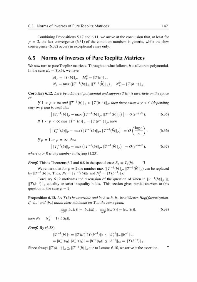
buch72005/10/5page 147

�

�

�

�

�

�

�

�

6.5. Norms of Inverses of Pure Toeplitz Matrices 147

Combining Propositions 5.17 and 6.11, we arrive at the conclusion that, at least forp = 2, the fast convergence (6.31) of the condition numbers is generic, while the slowconvergence (6.32) occurs in exceptional cases only.

6.5 Norms of Inverses of Pure Toeplitz MatricesWe now turn to pure Toeplitz matrices. Throughout what follows, b is a Laurent polynomial.In the case Bn = Tn(b), we have

Mp = ‖T (b)‖p, M0p = ‖T (b)‖p,

Np = max(‖T −1(b)‖p, ‖T −1(b)‖p

), N0

p = ‖T (b−1)‖p.

Corollary 6.12. Let b be a Laurent polynomial and suppose T (b) is invertible on the space�p.

If 1 ‖T (b−1)‖p, then there exists a γ > 0 (dependingonly on p and b) such that∣∣ ‖T −1

n (b)‖p −max(‖T −1(b)‖p, ‖T −1(b)‖p

) ∣∣ = O(e−γ√

n). (6.35)

If 1 < p <∞ and ‖T −1(b)‖p = ‖T (b−1)‖p, then∣∣ ‖T −1n (b)‖p −max

(‖T −1(b)‖p, ‖T −1(b)‖p

) ∣∣ = O

(log n

n

). (6.36)

If p = 1 or p = ∞, then∣∣ ‖T −1n (b)‖p −max

(‖T −1(b)‖p, ‖T −1(b)‖p

) ∣∣ = O(e−αn/2), (6.37)

where α > 0 is any number satisfying (1.23).

Proof. This is Theorems 6.7 and 6.8 in the special case Bn = Tn(b).

We remark that for p = 2 the number max (‖T −1(b)‖p, ‖T −1(b)‖p) can be replacedby ‖T −1(b)‖2. Thus, N2 = ‖T −1(b)‖2 and N0

2 = ‖T (b−1)‖2.

Corollary 6.12 motivates the discussion of the question of when in ‖T −1(b)‖p ≥‖T (b−1)‖p equality or strict inequality holds. This section gives partial answers to thisquestion in the case p = 2.

Proposition 6.13. Let T (b) be invertible and let b = b−b+ be a Wiener-Hopf factorization.If |b−| and |b+| attain their minimum on T at the same point,

mint∈T|b−(t)| = |b−(t0)|, min

t∈T|b+(t)| = |b+(t0)|, (6.38)

then N2 = N02 = 1/|b(t0)|.

Proof. By (6.38),

‖T −1(b)‖2 = ‖T (b−1+ )T (b−1

− )‖2 ≤ ‖b−1+ ‖∞‖b−1

− ‖∞= |b−1

+ (t0)| |b−1− (t0)| = |b−1(t0)| ≤ ‖b−1‖∞ = ‖T (b−1)‖2.

Since always ‖T (b−1)‖2 ≤ ‖T −1(b)‖2 due to Lemma 6.10, we arrive at the assertion.

buch72005/10/5page 148

�

�

�

�

�

�

�

�


Corollary 6.14. Suppose T (b) is invertible. If T (b) is Hermitian or triangular, thenN2 = N0

2 . Moreover, if t0 ∈ T is any point at which |b| attains its minimum on T, thenN2 = N0

2 = 1/|b(t0)|.

Proof. Let T (b) be Hermitian. Then b is real valued, and the invertibility of T (b) impliesthat b(t) ≥ ε > 0 or b(t) ≤ −ε < 0 for all t ∈ T. In the first case, log b is a real-valuedfunction in W . Therefore (log b)−k = (log b)k , whence

b−(t) := exp

(1

2(log b)0 +

∞∑k=1

(log b)−kt−k

)

= exp

(1

2(log b)0 +

∞∑k=1

(log b)ktk

)=: b+(t).

The factorization b = b−b+ is a Wiener-Hopf factorization. Since |b+| = |b−|, condition(6.38) is satisfied for some t0 ∈ T. Thus, N2 = N0

2 = 1/|b(t0)| by Proposition 6.13. Ifb(t) ≤ −ε < 0, we can apply the preceding argument to −b.

If T (b) is triangular, then T −1(b) = T (b−1), and this yields all assertions.

Theorem 6.15. Let P00 be the set of all Laurent polynomials that have no zeros on T andwhose winding number is zero. Equip P00 with the L∞ metric. The set of all b ∈ P00 forwhich N2 = ‖T −1(b)‖2 > ‖T (b−1)‖2 = N0

2 is an open and dense subset of P00.

Proof. It is clear that the set is open. To show that it is dense, pick b ∈ P00 and ε > 0.We construct a c ∈ P00 such that ‖c − b‖∞ < ε and ‖T −1(c)‖2 > ‖T (c−1)‖2. SinceT (μb(t/t0)) = μ diag (1, t0, t

20 , . . . ) T (b) diag (1, t−1

0 , t−20 , . . . ), we may without loss of

generality assume that mint∈T |b(t)| = 1 and b(1) = 1. Let 0 < δ < 1/4 and considerc = bϕ−δ ϕ+δ where

ϕ−δ (t) = 1− 2δ + 2δt−n

1− δ + δt−n, ϕ+δ (t) = 1− δ + δtn

1− 2δ + 2δtn.

Clearly, ‖c−b‖∞ < ε if only δ > 0 is sufficiently small. It is easy to see that |ϕ−δ (t)ϕ+δ (t)| =1 for all t ∈ T and that ϕ−δ (1) = ϕ+δ (1) = 1. Since ‖T (c−1)‖2 = ‖c−1‖∞ = 1, we are leftwith proving that ‖T −1(c)‖2 > 1.

Let b = b−b+ be a Wiener-Hopf factorization with b−(1) = b+(1) = 1. Then

c = c−c+, c− := b−ϕ−δ , c+ := b+ϕ+δ

is a Wiener-Hopf factorization of c. Given z ∈ C such that |z| > 1, put

fz(t) =√

1− 1

|z|2(

1− t

z

)−1

.

The sequence of the Fourier coefficients of fz is

xz :=√

1− 1

|z|2{

. . . , 0, 0, 1,1

z,

1

z2, . . .

}.

buch72005/10/5page 149

�

�

�

�

�

�

�

�


Thus, we may think of xz as a unit vector in �2. It is readily seen that T (d−)xz = d−(z)xz

for every d− ∈ W−. This implies that

‖T −1(c)xz‖22 = ‖T (c−1

+ )T (c−1− )xz‖2

2 = |c−1− (z)|2‖T (c−1

+ )xz‖22.

Using the analogue of Lemma 4.7 for infinite matrices, we get

‖T (c−1+ )xz‖2

2 = ‖c−1+ fz‖2

2

= ‖(c−1+ − c−1

+ (1/z))fz + c−1+ (1/z)fz‖2

2

= ‖(c−1+ − c−1

+ (1/z))fz‖22 + |c−1

+ (1/z)|2

+ 2

(1− 1

|z|2)

Re∫ 2π

0

(c−1+ (eiθ )− c−1

+ (1/z)) c−1+ (1/z)

(1− eiθ /z)(1− e−iθ /z)

dθ

2π.

The integral is the 0th Fourier coefficient of its integrand, and taking into account that[a+(eiθ )

1− eiθ /z

]0

=[(

a0 + a1eiθ + a2e

2iθ + · · · ) (1+ e−iθ

z+ e−2iθ

z2 + · · ·)]

0

= a0 + a1

z+ a2

z2 + · · · = a+(1/z),

we see that the integral is zero. Thus,

‖T −1(c)xz‖22 = |c−1

− (z)c−1+ (1/z)|2 + |c−1

− (z)|2 ‖(c−1+ − c−1

+ (1/z))fz‖22. (6.39)

Now put n = [1/δ3] and z = 1+ δ3. We have

1

ϕ−δ (z)= 1

ϕ−δ (1+ δ3)= 1+ δ(1− (1+ δ3)−n)

1− 2δ(1− (1+ δ3)−n)

and since (1+ 1/n)−n = e−1 +O(1/n) and hence (1+ δ3)−n = e−1 +O(δ3), we obtainthat

1

ϕ−δ (z)= 1+ δ(1− e−1)

1− 2δ(1− e−1)+O(δ4) = 1+ δ(1− e−1)+O(δ2). (6.40)

Analogously,

1

ϕ+δ (1/z)= 1− δ(1− e−1)

1− δ(1− e−1)+O(δ4) = 1− δ(1− e−1)+O(δ2). (6.41)

It is obvious that

ϕ−δ (z)ϕ+δ (1/z) = 1. (6.42)

Since z = z, equalities (6.39) and (6.42) imply that

‖T −1(c)xz‖22 = |b−1

− (z)b−1+ (1/z)|2 + |b−1

− (z)|2 |1/ϕ−δ (z)|2 ‖(c−1+ − c−1

+ (1/z))fz‖22.

buch72005/10/5page 150

�

�

�

�

�

�

�

�


The formulas

b−(z) = b−(1+ δ3) = 1+O(δ3), b+(1/z) = b+(1/(1+ δ3)) = 1+O(δ3)

together with (6.40) therefore give

‖T −1(c)xz‖22 = 1+O(δ3)+ (1+O(δ3))(1+O(δ)) ‖(c−1

+ − c−1+ (1/z))fz‖2

2. (6.43)

Further,

‖(c−1+ − c−1

+ (1/z))fz‖2 = ‖((ϕ+δ )−1b−1+ − (ϕ+δ )−1(1/z)b−1

+ (1/z))fz‖2

≥ ‖((ϕ+δ )−1 − (ϕ+δ )−1(1/z))b−1+ fz‖2 − |(ϕ+δ )−1(1/z)| ‖(b−1

+ − b−1+ (1/z))fz‖2

=: A− B.

We have

B2 = |(ϕ+δ )−1(1/z)|2(

1− 1

z2

)∫T

|b−1+ (t)− b−1

+ (1/z)|2|1− t/z|2

|dt |2π

= |(ϕ+δ )−1(1/z)|2(

1− 1

z2

)∫T

|b−1+ (t)− b−1

+ (1/z)|2|t − 1/z|2

|dt |2π

= |(ϕ+δ )−1(1/z)|2(

1− 1

z2

)∫T|gz(t)|2 |dt |

2π

with the function

gz(t) = b−1+ (t)− b−1

+ (1/z)

t − 1/z=

∞∑j=1

hj (t − 1/z)j .

The function gz is analytic in some open disk containing D. Thus, there is a constant M <∞such that ‖gz‖ ≤ M for all z sufficiently close to 1. Since, by (6.41), |(ϕ+δ )−1(1/z)|2 =1+O(δ) and, obviously, 1− 1/z2 = O(δ3), it follows that

B ≤ (1+O(δ)) O(δ3/2) M = O(δ3/2).

On the other hand,

A2 =(

1− 1

z2

)∫T

|(ϕ+δ )−1(t)− (ϕ+δ )−1(1/z)|2 |b−1+ (t)|2

|1− t/z|2|dt |2π

≥ γ 2

(1− 1

z2

)∫T

|(ϕ+δ )−1(t)− (ϕ+δ )−1(1/z)|2|1− t/z|2

|dt |2π

,

where γ = mint∈T |b−1+ (t)|. Taking into account (6.41) we get

(ϕ+δ )−1(t)− (ϕ+δ )−1(1/z) = 1− δ(1− tn)

1− δ(1− tn)− 1+ δ(1− 1/zn)

1− δ(1− 1/zn)

= δ

(1− tn

1− δ(1− tn)− 1− e−1

1− δ(1− e−1)+O(δ3)

)= δ(1− tn − (1− e−1)+O(δ))

= δ(e−1 − tn +O(δ))

buch72005/10/5page 151

�

�

�

�

�

�

�

�


and hence arrive at the estimate

A2 ≥ γ 2

(1− 1

z2

)δ2

∫T

(|tn − e−1| +O(δ))2

|1− t/z|2|dt |2π

≥ γ 2

(1− 1

z2

)δ2

∫T

(1− e−1 +O(δ))2

|1− t/z|2|dt |2π

= γ 2 δ2 (1− e−1 +O(δ))2 = γ 2 (1− e−1)2 δ2 +O(δ3).

In summary, (6.43) yields

‖T −1(c)xz‖2 ≥ 1+O(δ3)+ (1+O(δ))(A− B)2

≥ 1+O(δ3)+ (1+O(δ))(γ (1− e−1)δ +O(δ3/2))2

= 1+ γ 2 (1− e−1)2 δ2 +O(δ5/2),

and this is certainly greater than 1 if only δ > 0 is sufficiently small.

By virtue of Theorem 6.15, we may say that the strict inequality N2 > N02 is the

generic case, whereas the equality N2 = N02 represents the exceptional case. Corollary 6.14

tells us that we are in the exceptional case whenever T (b) is Hermitian or triangular.Estimates (6.35) and (6.36) result from our techniques, and it may be that these

estimates can be improved. We conjecture that Corollary 6.12 remains valid with the right-hand sides of (6.35) and (6.36) replaced by O(e−γ n) and O (1/n2), respectively. However,as the following example shows, the gap between (6.35) and (6.36) is essential and cannotbe removed.

Example 6.16. Let b(t) = 3 − t − t−1 (t ∈ T). By Theorem 2.4, the eigenvalues of theHermitian matrix Tn(b) are

λj (Tn(b)) = 3+ 2 cosjπ

n+ 1(j = 1, . . . , n).

This implies that

‖T −1n (b)‖2 = 1

λn(Tn(b))= 1− π2

n2+O

(1

n3

),

and it also shows that ‖T −1n (b)‖2 − ‖T −1(b)‖2 = ‖T −1

n (b)‖2 − 1 cannot decay faster thanO(1/n2).

Estimate (6.36) is universal in the sense that it does not depend on any further infor-mation about b. In case we know more about b, we can improve (6.36).

Lemma 6.17. Let b be a Laurent polynomial for which T (b) is invertible. Further, lett0 ∈ T be any point at which |b| attains its minimum and suppose that

|b(t)− b(t0)| ≤ D|t − t0|γ for all t ∈ T,

where D ∈ (0,∞) and γ ∈ N. Then

‖T −1n (b)‖2 ≥ ‖T (b−1)‖2 − C

nγfor all n ≥ 1

with some constant C ∈ (0,∞).

buch72005/10/5page 152

�

�

�

�

�

�

�

�


Proof. Without loss of generality assume that t0 = 1. Put j = γ + 1 and let m bethe nonnegative integer for which mj < n ≤ (m + 1)j . Define p

jm ∈ P+mj+1 by (4.20),

(4.21). Clearly, pjm ∈ P+n . To estimate ‖T −1

n (b)‖2, we make use of Lemma 4.9. We have‖bpj

m‖2 ≤ |b(1)| ‖pjm‖2 + ‖(b − b(1))p

jm‖2, and

‖(b − b(1))pjm‖2

2 =∫ π

−π

|b(eiθ )− b(1)|2(

sin((m+ 1)θ/2)

sin(θ/2)

)2jdθ

2π

= O

(∫|θ |<1/(m+1)

|θ |2γ (m+ 1)2j dθ

2π+

∫|θ |>1/(m+1)

|θ |2γ |θ |−2j dθ

2π

)= O

((m+ 1)2j

(m+ 1)2γ+1+ (m+ 1)2γ+1

(m+ 1)2j

)= O (m+ 1) = O(m).

Thus, by Lemma 4.10,

‖bpjm‖2

‖pjm‖2

≤ |b(1)| +O

(m1/2

mj−1/2

)= |b(1)| +O

(1

mγ

).

From Lemma 4.9 we now obtain that ‖T −1n (b)‖2 is at least

1

|b(1)| +O(1/mγ )= 1

|b(1)| +O(1/nγ )≥ 1

|b(1)| −O

(1

nγ

)≥ 1

|b(1)| − C1

nγ,

and since ‖T (b−1)‖2 = ‖b−1‖∞ = 1 / min |b| = 1/|b(1)|, we arrive at the assertion.

Theorem 6.18. Let b be a Laurent polynomial and suppose T (b) is invertible. Let t0 ∈ Tand assume

|b(t0)| = mint∈T|b(t)|, |b(t)− b(t0)| ≤ D|t − t0|γ (t ∈ T).

If T (b) is Hermitian or triangular, then N2 = ‖T (b−1)‖2 = 1/|b(t0)| and

N2

(1− C

nγ

)≤ ‖T −1

n (b)‖2 ≤ N2 for all n ≥ 1, (6.44)

where C ∈ (0,∞) is some constant independent of n.

Proof. The equalities N2 = ‖T (b−1)‖2 = 1/|b(t0)| follow from Corollary 6.14, and thelower estimate in (6.44) results from Lemma 6.17. To prove the upper estimate of (6.44),assume first that T (b) is Hermitian. Then b(t) ≥ |b(t0)| > 0 or b(t) ≤ −|b(t0)| < 0 for allt ∈ T. We consider the first case (the second case can be reduced to the first case by replacingb with −b). Let λmin be the smallest eigenvalue of Tn(b) and let x be an eigenvector suchthat ‖x‖2 = 1. Define f ∈ P+n by (4.15). Then, by (4.16),

λmin = (Tn(b)x, x) = 1

2π

∫ 2π

0b(eiθ )|f (eiθ )|2dθ ≥ |b(t0)|,

whence ‖T −1n (b)‖2 = 1/λmin ≤ 1/|b(t0)| = N2. This is the upper estimate of (6.44) for

Hermitian matrices. If T (b) is triangular, we have T −1n (b) = Tn(b

−1), which implies that‖T −1

n (b)‖2 = ‖Tn(b−1)‖2 ≤ ‖b−1‖∞ = 1/|b(t0)| = N2.

buch72005/10/5page 153

�

�

�

�

�

�

�

�

6.6. Condition Numbers of Pure Toeplitz Matrices 153

6.6 Condition Numbers of Pure Toeplitz MatricesCombining our results on the converge speed of norms and norms of inverses, we canestablish a result on the convergence speed for condition numbers.

Corollary 6.19. Let b be a Laurent polynomial and let T (b) be invertible on the space �p.If 1 0 is subject to (1.23).

Proof. In the case at hand, MpNp = max(κp(T (b)), κp(T (b))). Thus, (6.32) gives (6.45),while (6.33) yields (6.46).

Note that in the case p = 2 the equality max (κ2(T (b)), κ2(T (b))) = κ2(T (b)) holds.We emphasize that generically ‖T −1

n (b)‖p converges to Np very fast, namely, at leastof the order O(e−γ

√n). The generically slow convergence of κp(Tn(b)) to MpNp is caused

by the generically slow convergence of ‖Tn(b)‖p to Mp.As in the case of the norms of the inverses, we believe that (6.45) can be sharp-

ened. However, the following result shows that generically we cannot expect more thanpolynomially fast convergence.

Proposition 6.20. The set of all Laurent polynomials b ∈ P00 for which there exist constants2γ ∈ {2, 4, 6, . . . } and μ > 0 such that

| κ2(Tn(b))− κ2(T (b)) | ≥ μ

n2γfor all n ≥ 1

is an open and dense subset of P00.

Proof. Let

E1 = {b ∈ P00 : |b| is not constant}, E2 = {b ∈ P00 : ‖T −1(b)‖2 > ‖T (b−1)‖2}.Proposition 5.6 implies that E1 is open and dense, and Theorem 6.15 says that E2 is openand dense. Hence, E1 ∩ E2 is also an open and dense subset of P00. If b ∈ E1 ∩ E2, then

| ‖Tn(b)‖2 − ‖T (b)‖2 | ≥ c

n2γ,

∣∣ ‖T −1n (b)‖2 − ‖T −1(b)‖2

∣∣ ≤ de−δ√

n

by Theorem 5.8 and (6.35), whence

| κ2(Tn(b))− κ2(T (b)) | = ∣∣ ‖Tn(b)‖2 ‖T −1n (b)‖2 − ‖T (b)‖2 ‖T −1(b)‖2

∣∣≥ ‖T −1(b)‖2

∣∣∣ ‖Tn(b)‖2 − ‖T (b)‖2

∣∣∣− ‖Tn(b)‖2

∣∣∣ ‖T −1n (b)‖2 − ‖T −1(b)‖2

∣∣∣≥ ‖T −1(b)‖2 cn−2γ n − ‖Tn(b)‖2 de−δ

√n ≥ μn−2γ

for some μ > 0.

buch72005/10/5page 154

�

�

�

�

�

�

�

�


6.7 ConclusionsIn Chapters 5 and 6, we proved several estimates that make precise the following insights:

(a) Within the class of Toeplitz-like matrices, fast convergence of the norms, of thenorms of the inverses, and of the condition numbers is generic.

(b) Within the class of pure Toeplitz matrices, norms converge generically slow, normsof inverses converge generically fast, and condition numbers converge generically slow.

Exercises

1. Prove that there exist b, c ∈ P such that

‖T (b)T (c)‖2 < ‖T (c)T (b)‖2.

2. Let K = diag (0,−3/4, 0, 0, . . . ) and L = diag (2,−1/2, 0, 0, . . . ). Then for n ≥ 4,

An := I + PnKPn +WnLWn = diag(

1,1

4, 1, . . . , 1︸︷︷︸

n−4

,1

3, 3

).

Let A and A denote the strong limits of An and WnAnWn. Show that

limn→∞ κ2(An) = 12, κ2(A) = 4, max(κ2(A), κ2(A)) = 6.

3. Show that there exist b ∈ P such that κ2(Tn(b)) → ∞ as n → ∞ although‖Tn(b)‖2 ≤ 2 and det Tn(b) = 1 for all n ≥ 1.

4. Let {an}∞n=0 be a sequence of complex numbers satisfying |an| = O(1/n2) and put

An =

⎛⎜⎜⎜⎜⎜⎝0 0 . . . 0 a0

a0 0 . . . 0 a1

a1 a0 . . . 0 a2...

.... . .

......

an an−1 . . . a0 an+1

⎞⎟⎟⎟⎟⎟⎠ .

Fix p ∈ [1,∞]. Show that κp(An) remains bounded as n → ∞ if and only if∑∞n=0 anz

n �= 0 for |z| ≤ 1.

5. Find four Laurent polynomials a, b, c, d such that ad − bc has no zeros on T andwinding number zero but

κp

(Tn(a) Tn(b)

Tn(c) Tn(d)

)→∞ as n→∞

for every p ∈ [1,∞].6. Let b ∈ P and suppose b ≥ 0 on T and G(b) = 1. Prove that κ2(Tn(b))/Dn(b)

converges to zero if b has at least three distinct zeros on T. What can be said aboutthe ratio κ2(Tn(b))/Dn(b) if b has no, exactly one, or exactly two distinct zeros onT?

buch72005/10/5page 155

�

�

�

�

�

�

�

�

Notes 155

7. Let p(z) = p0 + · · · + pn−1zn−1 + zn (p0 �= 0) and suppose we know that p(z) has

m zeros in {z ∈ C : |z| < r < 1} and n−m zeros in {z ∈ C : |z| > R > 1}. We wanta polynomial factorization p(z) = v(z)�(z) such that all zeros of v(z) and �(z) areof modulus less than r and greater than R, respectively. To estimate the conditioningof this problem, let p(z) be another polynomial of the same form as p(z) and denoteby p(z) = v(z)�(z) the corresponding factorization.

(a) Prove that the coefficients of � are the solution x of the equation T (a−1)x = e1,where a(t) = t−mp(t) and e1 = {1, 0, 0, . . . }.(b) Prove that if ‖p − p‖∞ ≤ ε ‖p‖∞, then

‖�− �‖2

‖�‖2≤ ε κ2(T (a−1)) ‖p‖∞ ‖p−1‖∞ +O(ε2) as ε → 0,

where ‖ · ‖2 and ‖ · ‖∞ are the norms in L2(T) and L∞(T).

8. Let An be an n × n matrix with distinct eigenvalues λ1, . . . , λn. Choose nonzerovectors xj and yj such that Anxj = λjxj and A∗nyj = λjyj (j = 1, . . . , n). Theinstability index i(An) is defined as

i(An) = max1≤j≤n

‖xj‖2‖yj‖2

|(xj , yj )| .

(a) Prove the following implications:

V −1n AnVn is diagonal for some Vn with κ2(Vn) ≤ k

�⇒ ‖(An − λI)−1‖2 ≤ k/dist (λ, sp An) for all λ /∈ sp An

�⇒ i(An) ≤ k.

(b) Show that if

An =

⎛⎜⎜⎜⎝f0 fn−1a

−1 . . . f1a−(n−1)

f1a f0 . . . f2a−(n−2)

......

...

fn−1an−1 fn−2a

n−2 . . . f0

⎞⎟⎟⎟⎠with a > 1, then

i(An) = a

(a2 − 1)n(an − a−n).

Notes

Corollary 6.5 was established in [34] for p = 2 and in [146] for p = 1. Example 6.6 isfrom [146]. All other results of this chapter are taken from the papers [49], [59], [62]. Weremark that Theorem 6.15 is stated in [59] but that the proof given there is incorrect. Wethank Alexander Rogozhin for bringing this to our attention. The proof presented here isnew.

The result of Exercise 7 was established in [28]. Exercise 8 is from [95]. Note thatwhat is called the “instability index” in [95] and here is also known as the maximum of theeigenvalue condition numbers (see [298] and [137]).

buch72005/10/5page 156

�

�

�

�

�

�

�

�

buch72005/10/5page 157

�

�

�

�

�

�

�

�

Chapter 7

Substitutes forthe Spectrum

As will be seen in Chapter 11, the spectrum sp Tn(b) need not mimic sp T (b) as n goesto infinity. In contrast to this, pseudospectra and numerical ranges behave as nicely as wecould ever expect. These sets are the concern of the present chapter.

7.1 PseudospectraFor ε > 0, the ε-pseudospectrum of an operator A ∈ B(X) on a Banach space X is definedby

spεA ={λ ∈ C : ‖(A− λI)−1‖B(X) ≥ 1/ε

}. (7.1)

Here we put ‖(A− λI)−1‖B(X) = ∞ if A− λI is not invertible. Thus, the usual spectrumsp A is always a subset of spεA. Clearly, spεA depends on X. If A acts on �p or �

pn , we

denote the ε-pseudospectrum of A by sp(p)ε A.

Definition (7.1) admits several modifications and generalizations. An important gen-eralization, which is motivated by plenty of applications, is the so-called structured pseu-dospectrum. In this context we are given three operators A, B, C ∈ B(X) and we define

spB,Cε A = sp A ∪ {

λ /∈ sp A : ‖C(A− λI)−1B‖B(X) ≥ 1/ε}. (7.2)

Evidently, spεA is nothing but spI,Iε A. Furthermore, some authors prefer (7.1) and (7.2) with

“≥” replaced by “>”. Theorem 7.2 and its Corollary 7.3 will give alternative descriptionsof the sets (7.1) and (7.2) in the Hilbert space case.

Lemma 7.1. If M and N are linear operators, then I +MN is invertible if and only ifI +NM is invertible, in which case

(I +MN)−1 = I −M(I +NM)−1N.

Proof. Simply check that

(I +MN)(I −M(I +NM)−1N) = (I −M(I +NM)−1N)(I +MN) = I.

157

buch72005/10/5page 158

�

�

�

�

�

�

�

�

158 Chapter 7. Substitutes for the Spectrum

Theorem 7.2. If H is a Hilbert space, A, B, C ∈ B(H), and ε > 0, then⋃‖K‖≤ε

sp (A+ BKC) = sp A ∪ {λ /∈ sp A : ‖C(A− λI)−1B‖ ≥ 1/ε

}, (7.3)

⋃‖K‖<ε

sp (A+ BKC) = sp A ∪ {λ /∈ sp A : ‖C(A− λI)−1B‖ > 1/ε

}, (7.4)

the union taken over all K ∈ B(H) with the given norm constraint.

Proof. Suppose A is invertible and ‖CA−1B‖ ≤ 1/ε (respectively, ‖CA−1B‖ < 1/ε) and‖K‖ < ε (respectively, ‖K‖ ≤ ε). In either case, ‖CA−1BK‖ < 1, which implies thatI +CA−1BK is invertible. Using Lemma 7.1 with N = C and M = A−1BK , we see thatI +A−1BKC and thus also A+BKC = A(I +A−1BKC) are invertible. This proves thatthe left-hand sides of (7.3) and (7.4) are contained in the corresponding right-hand sides.

To show that the right-hand sides of (7.3) and (7.4) are subsets of the correspondingleft-hand sides, it suffices to prove that if A is invertible and ‖CA−1B‖ = 1/δ, then thereexists an operator K such that ‖K‖ = δ and A + BKC is not invertible. So assumethat A is invertible and ‖CA−1B‖ = 1/δ. Clearly, A + BKC = A(I + A−1BKC) isinvertible if and only if so is I + A−1BKC, which, by Lemma 7.1 with M = A−1B andN = KC, is equivalent to the invertibility of I +KCA−1B. Abbreviate CA−1B to S andput K = −δ2S∗. Then ‖K‖ = δ and I + KCA−1B = I − δ2S∗S. The spectral radiusof the positive semi-definite selfadjoint operator S∗S coincides with its norm, that is, with‖S∗S‖ = ‖S‖2 = 1/δ2. It follows that 1/δ2 ∈ sp S∗S. The spectral mapping theoremtherefore implies that 0 ∈ sp (I − δ2S∗S).

Corollary 7.3. Let H be a Hilbert space and A ∈ B(H). Then for every ε > 0,

spεA =⋃‖K‖≤ε

sp (A+K),

the union taken over all K ∈ B(H) of norm at most ε.

Proof. This is (7.3) with B = C = I .

The following result sharpens (7.4).

Theorem 7.4. Let X be a Banach space, let A, B, C be operators in B(X), and let ε > 0.Then

sp A ∪ {λ /∈ sp A : ‖C(A− λI)−1B‖ > 1/ε} (7.5)

=⋃‖K‖<ε

sp (A+ BKC) (7.6)

=⋃

‖K‖<ε, rank K=1

sp (A+ BKC). (7.7)

buch72005/10/5page 159

�

�

�

�

�

�

�

�

7.2. Norm of the Resolvent 159

Proof. The first part of the proof of Theorem 7.2 can literally be used to show that (7.6) isa subset of (7.5).

It remains to prove that (7.5) is contained in (7.7). This will follow as soon as we haveshown that if A is invertible and ‖CA−1B‖ > 1/ε, then there exists a rank-one operatorK such that ‖K‖ < ε and A + BKC is not invertible. So assume A is invertible and‖CA−1B‖ > 1/ε. Then we can find a u ∈ X such that ‖u‖ = 1 and ‖CA−1Bu‖ > 1/ε.Thus, ‖CA−1Bu‖ = 1/δ with δ < ε. By the Hahn-Banach theorem, there is a functionalϕ ∈ X∗ such that ‖ϕ‖ = 1 and ϕ(CA−1Bu) = ‖CA−1Bu‖ = 1/δ. Let K ∈ B(X) be therank-one operator defined by Kx = −δϕ(x)u. Clearly, ‖K‖ ≤ δ < ε. Furthermore,

BKCA−1Bu = B(−δϕ(CA−1Bu)u)

= −δϕ(CA−1Bu)Bu = −δ(1/δ)Bu = −Bu. (7.8)

Put y = A−1Bu. If y = 0, then CA−1Bu = Cy = 0, which contradicts the assumption‖CA−1Bu‖ = 1/δ > 0. Consequently, y �= 0. From (7.8) we see that BKCy = −Bu =−Ay, whence (A+ BKC)y = 0. This implies that A+ BKC is not invertible.

We have not been able to prove Theorem 7.4 with strict inequalities replaced bynonstrict inequalities. However, one can show that if X is a Banach space, A, B, C ∈ B(X),ε > 0, and at least one of the operators B or C is compact, then

sp A ∪ {λ /∈ sp A : ‖C(A− λI)−1B‖ ≥ 1/ε}

=⋃‖K‖≤ε

sp (A+ BKC) =⋃

‖K‖≤ε, rank K=1

sp (A+ BKC).

To see this, assume that A is invertible and ‖CA−1B‖ = 1/δ. Since CA−1B is compact,there exists a u ∈ X such that ‖u‖ = 1 and ‖CA−1Bu‖ = 1/δ. The rest of the proof is asin the proof of Theorem 7.4.

7.2 Norm of the ResolventIn this section we show that the norm of the resolvent of a bounded operator on �p (1 < p <

∞) cannot be locally constant. It should be noted that such a result is not true for arbitraryanalytic operator-valued functions. To see this, consider the function

A : C → B(�p

2 ), λ �→(

λ 00 1

).

Obviously, ‖A(λ)‖p = max(|λ|, 1) and thus ‖A(λ)‖p = 1 for all λ in the unit disk.

Theorem 7.5 (Daniluk). Let H be a Hilbert space and A ∈ B(H). Suppose that A − λI

is invertible for all λ in some open subset U of C. If there is an M < ∞ such that‖(A− λI)−1‖ ≤ M <∞ for all λ ∈ U , then ‖(A− λI)−1‖ < M for all λ ∈ U .

Proof. A little thought reveals that what we must show is the following: If U is an opensubset of C containing the origin and ‖(A− λI)−1‖ ≤ M for all λ ∈ U , then ‖A−1‖ < M .

buch72005/10/5page 160

�

�

�

�

�

�

�

�


To prove this, assume the contrary, i.e., let ‖A−1‖ = M . There is a sufficiently small r > 0such that

(A− λI)−1 =∞∑

j=0

λjA−j−1 for |λ| = r.

Given f ∈ H , we therefore get

‖(A− λI)−1f ‖2 =∑j,k≥0

λjλk(A−j−1f, A−k−1f )

whenever λ = reiϕ . Integrating the last equality we obtain

1

2π

∫ 2π

0‖(A− reiϕI )−1f ‖2dϕ =

∞∑j=0

r2j‖A−j−1f ‖2,

and since ‖(A− reiϕI )−1f ‖ ≤ M‖f ‖, it follows that ‖A−1f ‖2+ r2‖A−2f ‖2 ≤ M2‖f ‖2.Now pick an arbitrary ε > 0 and choose an fε ∈ H such that ‖fε‖ = 1 and ‖A−1fε‖2 >

M2 − ε. Then M2 − ε + r2‖A−2fε‖2 < M2, whence 1 = ‖fε‖2 ≤ ‖A2‖2‖A−2fε‖2 <

εr−2‖A2‖2, which is impossible if ε > 0 is small enough.

The following result extends Theorem 7.5 to operators on �p for 1 < p <∞.

Theorem 7.6. Let 1 < p <∞ and let A ∈ B(�p). If A− λI is invertible for all λ in someopen set U ⊂ C and ‖(A− λI)−1‖p ≤ M < ∞ for λ ∈ U , then ‖(A− λI)−1‖p < M forλ ∈ U .

Proof. We may without loss of generality assume that p ≥ 2; otherwise we can pass toadjoint operators. Again it suffices to show that ‖A−1‖p < M provided U contains theorigin. Assume the contrary, that is, let ‖A−1‖p = M . There is an r > 0 such that

(A− λI)−1 =∞∑

j=0

λjA−j−1

for all λ = reiϕ . Hence, for every x ∈ �p,

‖(A− λI)−1x‖pp =

∞∑n=0

∣∣∣∣∣∣∞∑

j=0

λj (A−j−1x)n

∣∣∣∣∣∣p

=∞∑

n=0

∣∣∣∣∣∣∞∑

j=0

rj eijϕ(A−j−1x)n

∣∣∣∣∣∣2p/2

=∞∑

n=0

∣∣∣∣∣∣( ∞∑

j=0

rj eijϕ(A−j−1x)n

)( ∞∑k=0

rke−ikϕ(A−k−1x)n

)∣∣∣∣∣∣p/2

=∞∑

n=0

∣∣∣∣∣C(r, n)+∞∑

�=1

B�(r, ϕ, n)

∣∣∣∣∣p/2

, (7.9)

buch72005/10/5page 161

�

�

�

�

�

�

�

�

7.2. Norm of the Resolvent 161

where

C(r, n) =∞∑

j=0

r2j |(A−j−1x)n|2,

B�(r, ϕ, n) = 2∞∑

k=0

r�+2kRe(ei�ϕ(A−�−k−1x)n(A−k−1x)n

).

For m = 0, 1, 2, . . . , put

Im(r, ϕ) =∞∑

n=0

∣∣∣∣∣C(r, n)+∞∑

�=1

B2m�(r, ϕ, n)

∣∣∣∣∣p/2

.

Clearly,

limm→∞ Im(r, ϕ) =

∞∑n=0

|C(r, n)|p/2. (7.10)

We now apply the inequality

|a|p/2 ≤ 1

2

(|a + b|p/2 + |a − b|p/2)

(7.11)

to

a = C(r, n)+∞∑

�=1

B2�(r, ϕ, n), b =∞∑

�=1

B2�−1(r, ϕ, n)

and sum up the results for n = 0, 1, 2, . . . . Taking into account that∑∞

n=0 |a − b|p/2 isnothing but I0(r, ϕ + π), we get

I1(r, ϕ) ≤ 1

2

(I0(r, ϕ)+ I0(r, ϕ + π)

). (7.12)

Letting

a = C(r, n)+∞∑

�=1

B4�(r, ϕ, n), b =∞∑

�=1

B4�−2(r, ϕ, n)

in (7.11), we analogously obtain that

I2(r, ϕ) ≤ 1

2

(I1(r, ϕ)+ I1(r, ϕ + π/2)

). (7.13)

Combining (7.12) and (7.13) we arrive at the inequality

I2(r, ϕ) ≤ 1

2

(I1(r, ϕ)+ I1(r, ϕ + π/2)

)≤ 1

4

(I0(r, ϕ)+ I0(r, ϕ + π/2)+ I0(r, ϕ + π)+ I0(r, ϕ + 3π/2)

). (7.14)

buch72005/10/5page 162

�

�

�

�

�

�

�

�


In the same way we see that

I3(r, ϕ) ≤ 1

2

(I2(r, ϕ)+ I2(r, ϕ + π/4)

),

which together with (7.14) gives

I3(r, ϕ) ≤ 1

8

7∑k=0

I0

(r, ϕ + kπ

4

).

Continuing this procedure we get

Im(r, ϕ) ≤ 1

2m

2m−1∑k=0

I0

(r, ϕ + kπ

2m−1

)(7.15)

for every m ≥ 0.Now put ϕ = 0 in (7.15) and pass to the limit m → ∞. The limit of the left-hand

side is given by (7.10). The right-hand side is an integral sum and hence

limm→∞

1

2m

2m−1∑k=0

I0

(r,

kπ

2m−1

)= lim

m→∞1

2π

2π

2m

∞∑k=0

I0

(r,

2kπ

2m

)= 1

2π

∫ 2π

0I0(r, ϕ)dϕ.

Thus,∞∑

n=0

|C(r, n)|p/2 ≤ 1

2π

∫ 2π

0I0(r, ϕ)dϕ.

Since ‖(A − λI)−1‖p ≤ M , we have I0(r, ϕ) = ‖(A − reiϕI )−1x‖pp ≤ Mp‖x‖p

p. Conse-quently,

∞∑n=0

|C(r, n)|p/2 ≤ Mp‖x‖pp. (7.16)

Because∞∑

n=0

|C(r, n)|p/2 ≥∞∑

n=0

∣∣∣ ∣∣(A−1x)n∣∣2 + r2

∣∣(A−2x)n∣∣2

∣∣∣p/2

≥∞∑

n=0

∣∣(A−1x)n∣∣p + rp

∞∑n=0

∣∣(A−2x)n∣∣p = ‖A−1x‖p

p + rp‖A−2x‖pp

(here we used the inequality (|a| + |b|)p/2 ≥ |a|p/2 + |b|p/2), we deduce from (7.16) that

‖A−1x‖pp + rp‖A−2x‖p

p ≤ Mp‖x‖pp. (7.17)

Finally, let ε > 0 and choose xε ∈ �p so that ‖xε‖p = 1 and ‖A−1x‖pp > Mp − ε. Then

(7.17) yields Mp − ε + rp‖A−2xε‖pp < Mp, and this implies that

1 = ‖xε‖pp ≤ ‖A2‖p

p‖A−2xε‖pp < εr−p‖A2‖p

p.

This inequality is impossible if ε > 0 is sufficiently small. Thus, our assumption ‖A−1‖p =M must be false.

buch72005/10/5page 163

�

�

�

�

�

�

�

�

7.3. Limits of Pseudospectra 163

7.3 Limits of PseudospectraLet {Mn}∞n=1 be a sequence of sets Mn ⊂ C. We define

lim infn→∞ Mn

as the set of all λ ∈ C for which there are λ1 ∈ M1, λ2 ∈ M2, . . . such that λn → λ, and welet

lim supn→∞

Mn

denote the set of all λ ∈ C for which there exist n1 < n2 < · · · and λnk∈ Mnk

such thatλnk

→ λ. In other words, λ ∈ lim inf Mn if and only if λ is the limit of some sequence{λn}∞n=1 with λn ∈ Mn, while λ ∈ lim sup Mn if and only if λ is a partial limit of sucha sequence. We remark that if M and the members of the sequence {Mn} are nonemptycompact subsets of C, then

lim infn→∞ Mn = lim sup

n→∞Mn = M

if and only if Mn converges to M in the Hausdorff metric, which means that d(Mn, M) → 0with

d(A,B) := max

(maxa∈A

dist (a, B), maxb∈B

dist (b, A)

).

This result is due to Hausdorff. Proofs can be found in [149, Sections 3.1.1 and 3.1.2] and[153, Section 2.8].

Theorem 7.7. Let b be a Laurent polynomial. Then for every ε > 0 and every p ∈ (1,∞),

lim infn→∞ sp(p)

ε Tn(b) = lim supn→∞

sp(p)ε Tn(b) = sp(p)

ε T (b) ∪ sp(p)ε T (b). (7.18)

Proof. We first show that

sp(p)ε T (b) ⊂ lim inf

n→∞ sp(p)ε Tn(b). (7.19)

If λ ∈ sp T (b), then ‖T −1n (b − λ)‖p → ∞ by virtue of Lemma 3.4. Thus, we have

‖T −1n (b − λ)‖p ≥ 1/ε for all n ≥ n0, which implies that λ ∈ sp(p)

ε Tn(b) for all n ≥ n0.Consequently, λ belongs to lim inf sp(p)

ε Tn(b).Now suppose that λ ∈ sp(p)

ε T (b) \ sp T (b). Then ‖T −1(b− λ)‖p ≥ 1/ε. Let U ⊂ Cbe any open neighborhood of λ. From Theorem 7.6 we deduce that there is a point μ ∈ U

such that ‖T −1(b − μ)‖p > 1/ε. Hence, we can find a natural number k0 such that

‖T −1(b − μ)‖p ≥ 1

ε − 1/kfor all k ≥ k0.

As U was arbitrary, it follows that there exists a sequence μ1, μ2, . . . such that μk ∈sp(p)

ε−1/kT (b) and μk → λ. For every invertible operator A ∈ B(�p),

‖A−1‖p = supx �=0

‖A−1x‖p

‖x‖p

= supy �=0

‖y‖p

‖Ay‖p

=(

infy �=0

‖Ay‖p

‖y‖p

)−1

. (7.20)

buch72005/10/5page 164

�

�

�

�

�

�

�

�


Since ‖T −1(b − μk)‖p ≥ 1/(ε − 1/k), it results that

inf‖y‖p=1‖T (b − μk)y‖p ≤ ε − 1/k.

Thus, there are yk ∈ �p such that ‖yk‖p = 1 and ‖T (b − μk)yk‖p < ε − 1/(2k). Clearly,‖Tn(b − μk)Pnyk‖p → ‖T (b − μk)yk‖p and ‖Pnyk‖p → ‖yk‖p = 1 as n→∞. Hence,

‖Tn(b − μk)Pnyk‖p

‖Pnyk‖p

< ε − 1/(3k)

for all n > n0(k). Again invoking (7.20) we see that

‖T −1n (b − μk)‖p > (ε − 1/(3k))−1 > 1/ε

and thus μk ∈ sp(p)ε Tn(b) for all n > n0(k). This implies that λ = lim μk belongs to

lim inf sp(p)ε Tn(b). At this point the proof of (7.19) is complete.

Repeating the above reasoning with b in place of b we get the inclusion

sp(p)ε T (b) ⊂ lim inf

n→∞ sp(p)ε Tn(b). (7.21)

As Tn(b − λ) = WnTn(b − λ)Wn and Wn is an isometry of �pn , it is clear that sp(p)

ε Tn(b) =sp(p)

ε Tn(b). Thus, in (7.21) we may replace the Tn(b) on the right by Tn(b), which inconjunction with (7.19) proves that sp(p)

ε T (b)∪sp(p)ε T (b) is contained in lim inf sp(p)

ε Tn(b).We are left to prove the inclusion

lim supn→∞

sp(p)ε Tn(b) ⊂ sp(p)

ε T (b) ∪ sp(p)ε T (b). (7.22)

So let λ /∈ sp(p)ε T (b) ∪ sp(p)

ε T (b). Then ‖T −1(b− λ)‖p < 1/ε and ‖T −1(b− λ)‖p < 1/ε,whence, by Theorem 6.3,

‖T −1n (b − λ)‖p < 1/ε − δ < 1/ε for all n ≥ n0 (7.23)

with some δ > 0. If |μ− λ| is sufficiently small, then Tn(b−μ) is invertible together withTn(b − λ), and we have, from the first resolvent identity,

‖T −1n (b − μ)‖p ≤ ‖T −1

n (b − λ)‖p

1− |μ− λ| ‖T −1n (b − λ)‖p

. (7.24)

Let |μ− λ| < εδ(1/ε − δ)−1. In this case (7.23) and (7.24) give

‖T −1n (b − μ)‖p <

1/ε − δ

1− εδ(1/ε − δ)−1(1/ε − δ)= 1

ε.

Thus, μ /∈ sp(p)ε Tn(b) for n ≥ n0. This shows that λ cannot belong to the left-hand side of

(7.22).

Corollary 7.8. If b is a Laurent polynomial and ε > 0, then

lim infn→∞ sp(2)


sp(2)ε Tn(b) = sp(2)

ε T (b).

buch72005/10/5page 165

�

�

�

�

�

�

�

�

7.4. Pseudospectra of Infinite Toeplitz Matrices 165

Proof. Since T (b) is simply the transpose of T (b), the two norms ‖T −1(b − λ)‖2 and‖T −1(b−λ)‖2 coincide. Therefore sp(2)

ε T (b) = sp(2)ε T (b). The assertion is now immediate

from Theorem 7.7.

Figures 7.1 and 7.2 show an example with the symbol b(t) = −(6 − 13i)t + (5 −4i)t2 + 3t3 − (4+ 3i)t−2 + 3t−3.

7.4 Pseudospectra of Infinite Toeplitz MatricesFor every operator A ∈ B(�2) the inequality

1/dist (λ, sp A) ≤ ‖(A− λI)−1‖2 (7.25)

holds. This implies that ‖(A−λI)−1‖2 ≥ 1/ε whenever dist (λ, sp A) ≤ ε and hence yieldsthe universal lower estimate

sp A+ ε D ⊂ sp(2)ε A.

For Toeplitz operators, Theorem 4.29 gives

‖(T (a)− λI)−1‖2 = ‖T −1(a − λ)‖2 ≤ 1/dist (λ, convR(a)). (7.26)

Consequently, if dist (λ, convR(a)) > ε then ‖T −1(a − λ)‖2 < 1/ε and λ cannot belongto sp(2)

ε T (a). We therefore arrive at the upper estimate

sp(2)ε T (a) ⊂ convR(a)+ ε D.

Given a ∈ W , let V (a) be the set of all λ ∈ C \ sp T (a) for which

dist (λ, sp T (a)) = dist (λ, convR(a)).

From (7.25) and (7.26) we infer that if λ ∈ V (a), then

‖T −1(a − λ)‖2 = 1/dist (λ, convR(a))

and hence in V (a) the level curves ‖T −1(a − λ)‖2 = 1/ε coincide with the curvesdist (λ, convR(a)) = ε. If V (a) = C \ sp T (a), or equivalently, if sp T (a) is a convex set,then

sp(2)ε T (a) = convR(a)+ ε D. (7.27)

Equality (7.27) is particularly true for tridiagonal Toeplitz matrices, in which case sp T (a) =convR(a) is an ellipse.

7.5 Numerical RangeLet X be a Banach space and put

�(X) = {(f, x) ∈ X∗ ×X : ‖f ‖ = 1, ‖x‖ = 1, f (x) = 1}.

buch72005/10/5page 166

�

�

�

�

�

�

�

�


−20 −10 0 10 20−30

−25

−20

−15

−10

−5

0

5

10

15

20

−20 −10 0 10 20−30

−25

−20

−15

−10

−5

0

5

10

15

20

−20 −10 0 10 20−30

−25

−20

−15

−10

−5

0

5

10

15

20

−20 −10 0 10 20−30

−25

−20

−15

−10

−5

0

5

10

15

20

−20 −10 0 10 20−30

−25

−20

−15

−10

−5

0

5

10

15

20

−20 −10 0 10 20−30

−25

−20

−15

−10

−5

0

5

10

15

20

Figure 7.1. In the two top pictures we see b(T) (left) and b(T) together with the 100eigenvalues of T100(b) (right). The other four pictures indicate sp(2)

ε Tn(b) for ε = 1/100 andn = 50, 100, 150, 200. Each picture shows the superposition of the spectra sp (Tn(b)+E)

for 50 randomly chosen matrices E with ‖E‖2 = ε.

buch72005/10/5page 167

�

�

�

�

�

�

�

�

7.5. Numerical Range 167

−20 0 20

−30

−20

−10

0

10

20

−20 0 20

−30

−20

−10

0

10

20

−20 0 20

−30

−20

−10

0

10

20

−20 0 20

−30

−20

−10

0

10

20

Figure 7.2. These pictures were done by Mark Embree. In contrast to the lower fourpictures of Figure 7.1, the solid curves are the boundaries of the pseudospectra sp(2)

ε Tn(b)

for ε = 1/100 and n = 50, 100, 150, 200. These curves were determined with the help ofTom Wright’s package [299].

The (spatial) numerical range (= field of values) HX(A) of an operator A ∈ B(X) is definedas

HX(A) = {f (Ax) : (f, x) ∈ �(X)}.If X = H is a Hilbert space, we can identify the dual space X∗ with H and, accordingly,

�(H) = {(y, x) ∈ H ×H : ‖y‖ = 1, ‖x‖ = 1, (y, x) = 1}.Since equality holds in the Cauchy-Schwarz inequality |(y, x)| ≤ ‖y‖ ‖x‖ if and only if y

and x are linearly dependent, we see that actually

�(H) = {(x, x) ∈ H ×H : ‖x‖ = 1}.This implies that in the Hilbert space case the numerical range may also be defined by

HH (A) = {(Ax, x) : ‖x‖ = 1}.

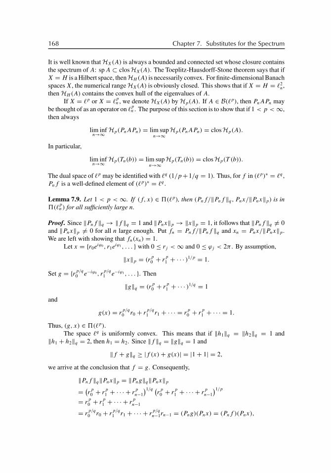
buch72005/10/5page 168

�

�

�

�

�

�

�

�


It is well known that HX(A) is always a bounded and connected set whose closure containsthe spectrum of A: sp A ⊂ closHX(A). The Toeplitz-Hausdorff-Stone theorem says that ifX = H is a Hilbert space, thenHH (A) is necessarily convex. For finite-dimensional Banachspaces X, the numerical range HX(A) is obviously closed. This shows that if X = H = �2

n,then HH (A) contains the convex hull of the eigenvalues of A.

If X = �p or X = �pn , we denote HX(A) by Hp(A). If A ∈ B(�p), then PnAPn may

be thought of as an operator on �pn . The purpose of this section is to show that if 1 < p <∞,

then always

lim infn→∞ Hp(PnAPn) = lim sup

n→∞Hp(PnAPn) = closHp(A).

In particular,

lim infn→∞ Hp(Tn(b)) = lim sup

n→∞Hp(Tn(b)) = closHp(T (b)).

The dual space of �p may be identified with �q (1/p+1/q = 1). Thus, for f in (�p)∗ = �q ,Pnf is a well-defined element of (�p)∗ = �q .

Lemma 7.9. Let 1 < p < ∞. If (f, x) ∈ �(�p), then (Pnf/‖Pnf ‖q, Pnx/‖Pnx‖p) is in�(�

pn) for all sufficiently large n.

Proof. Since ‖Pnf ‖q → ‖f ‖q = 1 and ‖Pnx‖p → ‖x‖p = 1, it follows that ‖Pnf ‖q �= 0and ‖Pnx‖p �= 0 for all n large enough. Put fn = Pnf/‖Pnf ‖q and xn = Pnx/‖Pnx‖p.We are left with showing that fn(xn) = 1.

Let x = {r0eiϕ0 , r1e

iϕ1 , . . . } with 0 ≤ rj <∞ and 0 ≤ ϕj < 2π . By assumption,

‖x‖p = (rp

0 + rp

1 + · · · )1/p = 1.

Set g = {rp/q

0 e−iϕ0 , rp/q

1 e−iϕ1 , . . . }. Then

‖g‖q = (rp

0 + rp

1 + · · · )1/q = 1

and

g(x) = rp/q

0 r0 + rp/q

1 r1 + · · · = rp

0 + rp

1 + · · · = 1.

Thus, (g, x) ∈ �(�p).The space �q is uniformly convex. This means that if ‖h1‖q = ‖h2‖q = 1 and

‖h1 + h2‖q = 2, then h1 = h2. Since ‖f ‖q = ‖g‖q = 1 and

‖f + g‖q ≥ |f (x)+ g(x)| = |1+ 1| = 2,

we arrive at the conclusion that f = g. Consequently,

‖Pnf ‖q‖Pnx‖p = ‖Png‖q‖Pnx‖p

= (r

p

0 + rp

1 + · · · + rp

n−1

)1/q (r

p

0 + rp

1 + · · · + rp

n−1

)1/p

= rp

0 + rp

1 + · · · + rp

n−1

= rp/q

0 r0 + rp/q

1 r1 + · · · + rp/q

n−1rn−1 = (Png)(Pnx) = (Pnf )(Pnx),

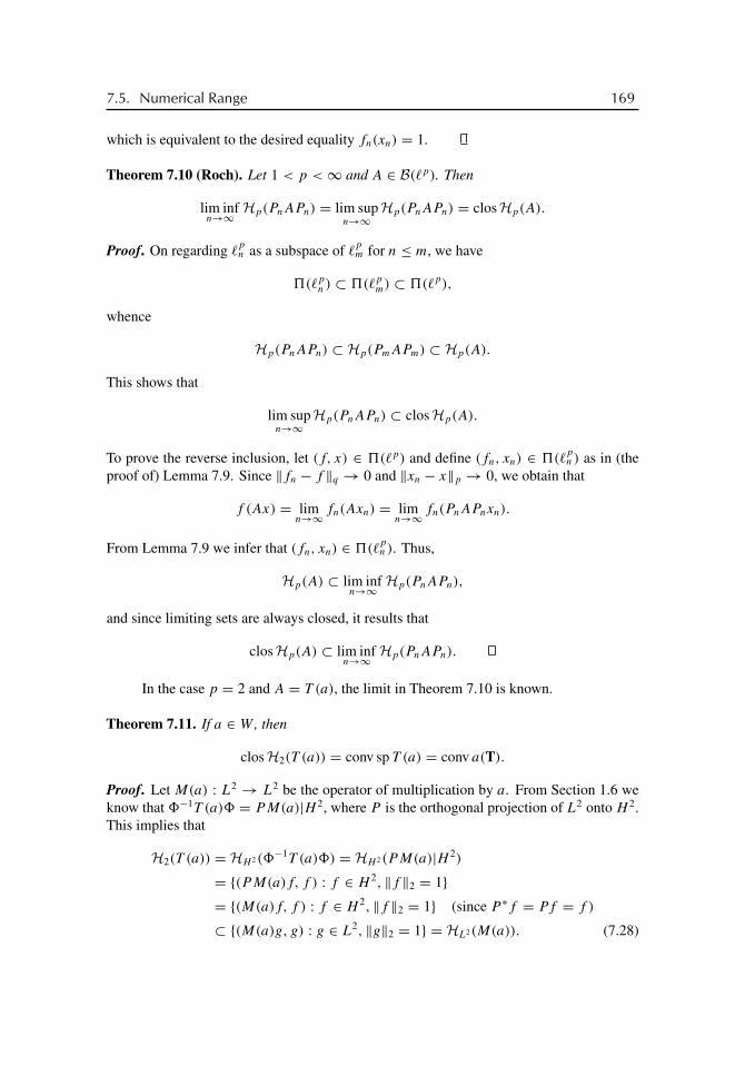
buch72005/10/5page 169

�

�

�

�

�

�

�

�

7.5. Numerical Range 169

which is equivalent to the desired equality fn(xn) = 1.

Theorem 7.10 (Roch). Let 1 < p <∞ and A ∈ B(�p). Then

lim infn→∞ Hp(PnAPn) = lim sup

n→∞Hp(PnAPn) = closHp(A).

Proof. On regarding �pn as a subspace of �

pm for n ≤ m, we have

�(�pn) ⊂ �(�p

m) ⊂ �(�p),

whence

Hp(PnAPn) ⊂ Hp(PmAPm) ⊂ Hp(A).

This shows that

lim supn→∞

Hp(PnAPn) ⊂ closHp(A).

To prove the reverse inclusion, let (f, x) ∈ �(�p) and define (fn, xn) ∈ �(�pn) as in (the

proof of) Lemma 7.9. Since ‖fn − f ‖q → 0 and ‖xn − x‖p → 0, we obtain that

f (Ax) = limn→∞ fn(Axn) = lim

n→∞ fn(PnAPnxn).

From Lemma 7.9 we infer that (fn, xn) ∈ �(�pn). Thus,

Hp(A) ⊂ lim infn→∞ Hp(PnAPn),

and since limiting sets are always closed, it results that

closHp(A) ⊂ lim infn→∞ Hp(PnAPn).

In the case p = 2 and A = T (a), the limit in Theorem 7.10 is known.

Theorem 7.11. If a ∈ W , then

closH2(T (a)) = conv sp T (a) = conv a(T).

Proof. Let M(a) : L2 → L2 be the operator of multiplication by a. From Section 1.6 weknow that �−1T (a)� = PM(a)|H 2, where P is the orthogonal projection of L2 onto H 2.This implies that

H2(T (a)) = HH 2(�−1T (a)�) = HH 2(PM(a)|H 2)

= {(PM(a)f, f ) : f ∈ H 2, ‖f ‖2 = 1}= {(M(a)f, f ) : f ∈ H 2, ‖f ‖2 = 1} (since P ∗f = Pf = f )

⊂ {(M(a)g, g) : g ∈ L2, ‖g‖2 = 1} = HL2(M(a)). (7.28)

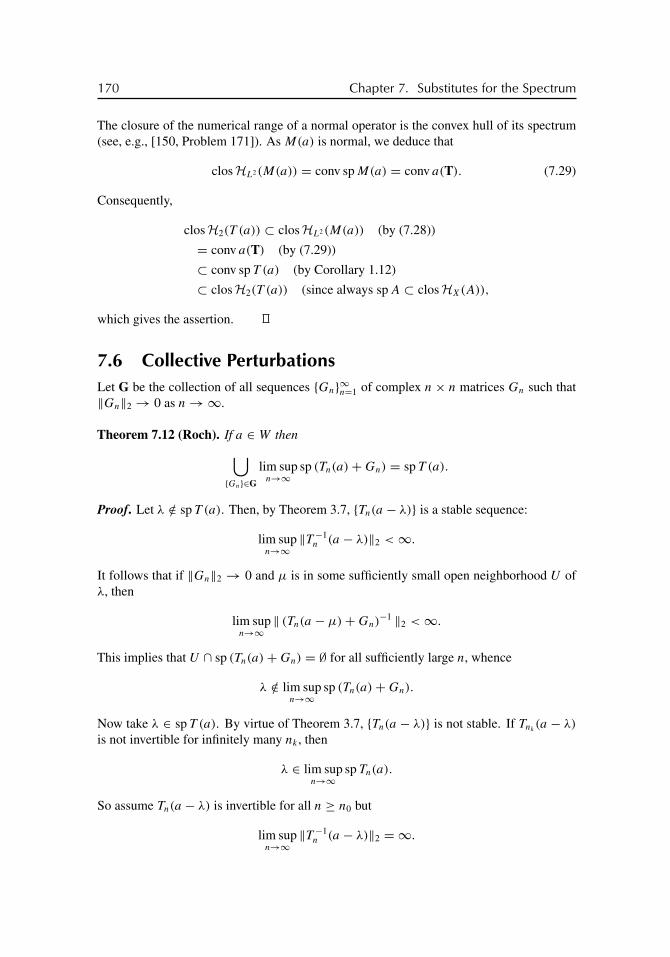
buch72005/10/5page 170

�

�

�

�

�

�

�

�


The closure of the numerical range of a normal operator is the convex hull of its spectrum(see, e.g., [150, Problem 171]). As M(a) is normal, we deduce that

closHL2(M(a)) = conv sp M(a) = conv a(T). (7.29)

Consequently,

closH2(T (a)) ⊂ closHL2(M(a)) (by (7.28))

= conv a(T) (by (7.29))

⊂ conv sp T (a) (by Corollary 1.12)

⊂ closH2(T (a)) (since always sp A ⊂ closHX(A)),

which gives the assertion.

7.6 Collective PerturbationsLet G be the collection of all sequences {Gn}∞n=1 of complex n × n matrices Gn such that‖Gn‖2 → 0 as n→∞.

Theorem 7.12 (Roch). If a ∈ W then⋃{Gn}∈G

lim supn→∞

sp (Tn(a)+Gn) = sp T (a).

Proof. Let λ /∈ sp T (a). Then, by Theorem 3.7, {Tn(a − λ)} is a stable sequence:

lim supn→∞

‖T −1n (a − λ)‖2 <∞.

It follows that if ‖Gn‖2 → 0 and μ is in some sufficiently small open neighborhood U ofλ, then

lim supn→∞

‖ (Tn(a − μ)+Gn)−1 ‖2 <∞.

This implies that U ∩ sp (Tn(a)+Gn) = ∅ for all sufficiently large n, whence

λ /∈ lim supn→∞

sp (Tn(a)+Gn).

Now take λ ∈ sp T (a). By virtue of Theorem 3.7, {Tn(a − λ)} is not stable. If Tnk(a − λ)

is not invertible for infinitely many nk , then

λ ∈ lim supn→∞

sp Tn(a).

So assume Tn(a − λ) is invertible for all n ≥ n0 but

lim supn→∞

‖T −1n (a − λ)‖2 = ∞.

buch72005/10/5page 171

�

�

�

�

�

�

�

�

Exercises 171

There are n1 < n2 < n3 < · · · and xnk∈ �2

nksuch that

‖xnk‖2 = 1 and ‖T −1

nk(a − λ)xnk

‖2 ≥ k.

Put ynk= T −1

nk(a − λ)xnk

and let Gnkbe the matrix of the linear operator

Gnk: �2

nk→ �2

nk, z �→ − (z, ynk

)xnk

‖ynk‖2

2

.

Obviously,

‖Gnk‖2 = sup

‖z‖2=1

|(z, ynk)| ‖xnk

‖2

‖ynk‖2

2

≤ ‖xnk‖2

‖ynk‖2≤ 1

k.

Let Gn = 0 for n ∈ N \ {n1, n2, . . . }. Then {Gn} ∈ G. Since(Tnk

(a)+Gnk− λI

)ynk= Tnk

(a − λ)ynk+Gnk

ynk= xnk

− xnk= 0,

it follows that Tnk+Gnk

− λI is not invertible. Hence

λ ∈ lim supn→∞

sp (Tn(a)+Gn).

Exercises

1. Let K be a compact operator on �2. Prove that

lim infn→∞ sp (I + PnKPn) = lim sup

n→∞sp (I + PnKPn) = sp (I +K).

2. Let a and b satisfy 0 < a ≤ b ≤ ∞. Show that there exists a selfadjoint operatorA ∈ B(�2) such that

‖A−1‖2 = a and lim supn→∞

‖(PnAPn)−1Pn‖2 = b.

3. Let A be a selfadjoint operator on �2 and suppose that spessA is a connected set. PutAn = PnAPn|Im Pn. Prove that

lim infn→∞ sp An = lim sup

n→∞sp An = sp A,

limn→∞‖(An − λI)−1‖2 = ‖(A− λI)−1‖2 (λ ∈ C \ sp A).

4. For m ≥ 0, let A : �2 → �2 be the operator

A : {x0, x1, x2, . . . } �→ {xm, xm+1, . . . }.Prove that sp(2)

ε A = (1+ ε)D.

buch72005/10/5page 172

�

�

�

�

�

�

�

�


5. Let m ≥ 2 and b(t) = t + t−m/m. Find the set V (b) and show that

{λ ∈ V (b) : ‖T −1(b − λ)‖2 = 1/ε}is the union of n+ 1 pure circular arcs of curvature 1/ε.

6. Let An be an n× n matrix and put

R′i (An) =⎛⎝ n∑

j=1

|aij |⎞⎠− |aii |.

Show that

sp(p)ε (An) ⊂

n⋃i=1

{λ ∈ C : |λ− aii | ≤ R′i (An)+ εn}.

7. Let ε > 0. Show that there exist Laurent polynomials b and c such that

sp T (b)+ εD �= sp(2)ε T (b), sp(2)

ε T (c) �= convR(c)+ εD.

8. Show that there exist finite matrices A and B such that

‖(λI − A)−1‖2 = ‖(λI − B)−1‖2 for all λ ∈ C

but ‖p(A)‖2 �= ‖p(B)‖2 for some polynomial p.

9. Show that the numerical range is robust in the following sense: If E ∈ B(X) and‖E‖ ≤ ε, then HX(A+ E) ⊂ HX(A)+ εD.

10. Let A be an n× n matrix. The numbers

αH(A) = maxλ∈H2(A)

Re λ, α(A) = maxλ∈sp A

Re λ

are called the numerical and spectral abscissas of A, respectively. Prove that

limt→0+0

d

dtlog ‖etA‖2 = αH(A), lim

t→+∞d

dtlog ‖etA‖2 = α(A).

11. Let a, b ∈ P\{0} and suppose that a0 = b0 = 0. Prove that the equality Tn(a)Tn(b) =0 is impossible for n ≤ 3 but possible for n ≥ 4.

Notes

Embree and Trefethen’s Web page [110] and book [275] are inexhaustible sources on allaspects of pseudospectra. The first chapter of [275] is on eigenvalues and it ends as follows:“In the highly nonnormal case, vivid though the image may be, the location of the eigenvaluesmay be as fragile an indicator of underlying character as the hair color of a Hollywood actor.

buch72005/10/5page 173

�

�

�

�

�

�

�

�

Notes 173

We shall see that pseudospectra provide equally compelling images that may capture thespirit underneath more robustly.”

“In summary, eigenvalues and eigenfunctions have a distinguished history of appli-cation throughout the mathematical sciences; we could not get around without them. Theirclearest successes, however, are associated with problems that involve well-behaved sys-tems of eigenvectors, which in most contexts means matrices or operators that are normalor nearly so. This class encompasses the majority of applications, but not all of them.For nonnormal problems, the record is less clear, and even the conceptual significance ofeigenvalues is open to question.”

As for the history of pseudospectra, we take the liberty of citing Trefethen and Embree[275] again. “These data suggest that the notion of pseudospectra has been invented at leastfive times:

J. M. Varah 1967 r-approximate eigenvalue1979 ε-spectrum

H. J. Landau 1975 ε-approximate eigenvaluesS. K. Godunov et al. 1975 spectral portraitL. N. Trefethen 1990 ε-pseudospectrumD. Hinrichsen and A. J. Pritchard 1992 spectral value set

One should not trust this table too far, however, as even recent history is notoriously hard topin down. It is entirely possible that Godunov or Wilkinson thought about pseudospectrain the 1960s, and indeed von Neumann may have thought about them in the 1930s. Norwere others such as Dunford and Schwartz, Gohberg, Halmos, Kato, Keldysch, or Kreissfar away.”

The infinite Toeplitz matrix T (b) is normal if and only if the essential range of b

is a line segment in the complex plane [77]. Consequently, infinite Toeplitz matrices aretypically nonnormal and hence pseudospectra are expected to tell us more about them thanspectra. The pioneering work on pseudospectra of Toeplitz matrices is the paper [219] byReichel and Trefethen. This paper was the source of inspiration for one of the authors’paper[34] and thus for investigations that have essentially resulted in large parts of the presentbook.

For B = C = I , that is, in the unstructured case, Theorems 7.2 and 7.4 are in principlealready in [269], [270]. In the structured case, these theorems are due to Hinrichsen, Kelb,Pritchard, and Gallestey [124], [125], [162], [163]. Section 7.1 is based on ideas of [125]and follows our paper [50].

The question whether the resolvent norm ‖(A−λI)−1‖may be locally constant arosein connection with [34]. One of the authors (A. B.) posed this question as an open problemat a Banach semester in Warsaw in 1994, and a few weeks later, Andrzej Daniluk of Cracowwas able to solve the problem. The proof of Theorem 7.5 is due to him. Theorem 7.6 wasestablished in [62].

Corollary 7.8, that is, Theorem 7.7 for p = 2, is due to Landau [185], [186], [187]and Reichel and Trefethen [219]. The first clean proof of this result was given in [34]. Forgeneral p ∈ (1,∞), Theorem 7.7 was proved in [62].

The (Hilbert space) numerical range HH (A) was introduced by Otto Toeplitz [268].For more on numerical ranges, in particular for proofs of the properties quoted in the text,we refer to the books [30], [148], [150], [167], [275]. Theorem 7.10 was established by

buch72005/10/5page 174

�

�

�

�

�

�

�

�


Roch [220]. Theorem 7.12 is also Roch’s; it appeared first in [149, Theorem 3.19]. Theorem7.11 and the proof given here are due to Halmos [150]. This theorem gives us the closure ofH2(T (b)). The set H2(T (b)) itself was determined by Klein [180]. There are two theoremsin [180]. Theorem 1 says that if the Toeplitz operator has a nonconstant symbol and isnormal so that the spectrum is a closed interval [γ, δ] ⊂ C, then the numerical range isthe corresponding open interval (γ, δ). Theorem 2 states that if the Toeplitz operator isnot normal, then its numerical range is the interior of the convex hull of its spectrum. Weremark that Halmos and Klein’s results are actually true for arbitrary b ∈ L∞.

We will say more on the numerical range of finite Toeplitz matrices in the notes toChapter 8.

Exercise 6 is from [111]. For Exercise 7 see [71]. Exercise 8 is a result by Greenbaumand Trefethen [144] (and can also be found in [275]). A solution to Exercise 10, which showsthat αH(A) and α(A) give the initial and final slope of the curve t �→ log ‖etA‖2, is in [275],for example. Exercise 11 is from [147].

Further results: convergence speed. Let b be a Laurent polynomial. If λ is in C \ b(T)

and wind (b, λ) �= 0, then ‖T −1n (b − λ)‖2 goes to infinity at least exponentially due to

Theorem 4.1. This implies that the inequality ‖T −1n (b− λ)‖2 ≥ 1/ε is already satisfied for

n’s of moderate size, and consequently, the convergence of sp(2)ε Tn(b) to sp(2)

ε T (b), whichis ensured by Corollary 7.8, is very fast. In [34], it is shown that Corollary 7.8 remains truefor dense Toeplitz matrices provided the symbol b is piecewise continuous. It was observedin [45] that in the case of piecewise continuous symbols the convergence of sp(2)

ε Tn(b) tosp(2)

ε T (b) may be spectacularly slow, which has its reason in the fact that ‖T −1n (b − λ)‖2

may grow only polynomially. The main result of our paper [54] says that such a slowconvergence of pseudospectra is generic even within the class of continuous symbols. In[54], we proved the following. Let b ∈ C2 and let λ ∈ C be a point whose winding numberwith respect to b(T) is−1 (respectively, 1). Then ‖T −1

n (b−λ)‖2 increases faster than everypolynomial,

limn→∞‖T

−1n (b − λ)‖2 n−β = ∞ for each β > 0,

if and only if Pb (respectively, Qb) is in C∞. Here (Pb)(t) :=∑∞j=0 bj t

j and (Qb)(t) :=∑−1j=−∞ bj t

j for b(t) =∑∞j=−∞ bj t

j .

Further results: operator polynomials. Roch [221] considered the polynomials

Ln(λ) = Tn(b0)+ Tn(b1)λ+ · · · + Tn(bk)λk,

L∞(λ) = T (b0)+ T (b1)λ+ · · · + T (bk)λk,

thought of as acting on �2n and �2, respectively, and proved that if T (bk) is invertible, then

lim infn→∞ {λ ∈ C : ‖L−1

n (λ)‖2 ≥ 1/ε} = lim supn→∞

{λ ∈ C : ‖L−1n (λ)‖2 ≥ 1/ε}

= {λ ∈ C : ‖L−1∞ (λ)‖2 ≥ 1/ε}

for each ε > 0.

buch72005/10/5page 175

�

�

�

�

�

�

�

�

Notes 175

Further results: higher order relative spectra. Let A ∈ B(�2) and let L be a closedsubspace of �2. We denote by PL the orthogonal projection of �2 onto L. For a naturalnumber k, the kth order spectrum spk(A, L) of A relative to L is defined as the set of allλ ∈ C for which the compression PL(A− λI)kPL|L is not invertible on L. This definitionis due to Brian Davies [94], who suggested that second order spectra might be useful forthe approximate computation of spectra of self-adjoint operators.

Shargorodsky’s paper [252] is devoted to the geometry of spk(A, L) for fixed L and tothe limiting behavior of spk(A, Ln) as PLn

converges strongly to the identity operator. Onemain result is a purely geometric description of the minimal setQk(K) with the property thatspk(A, L) ⊂ Qk(K) whenever A is a normal operator with sp A ⊂ K . Let, for example, K

be a compact subset of R. Put a = min K and b = max K . The set (a, b) \K is an at mostcountable union of open intervals, that is, of the form ∪j (aj , bj ). Let B(c1, c2) denote theclosed disk with diameter [c1, c2]. Then

Q2(K) = B(a, b) \⋃j

Int B(aj , bj ),

where Int stands for the interior points.Another remarkable result of [252] states that if A is normal, then⋃

{Ln}lim sup

n→∞spk(A, Ln) = sp A ∪Qk(spessA),

where spessA is the essential spectrum of A and the union is over all sequences {Ln} forwhich PLn

converges strongly to the identity operator. As a consequence, Shargorodskyobtains that if k is even, then⋃

{Ln}lim sup

n→∞spk(A, Ln) ∩ R = sp A

for every selfadjoint operator A. (In the last two equalities, lim sup may be replaced bylim inf.) This shows that, in contrast to usual spectra, even order relative spectra do notdeliver spurious points in the gaps of spessA when employing a projection method for theapproximate computation of sp A. For an arbitrary bounded operator A, the estimate

⋃{Ln}

lim supn→∞

spk(A, Ln) ⊂ sp A ∪ ‖A‖ess

sin(π/(2k))D

is proved in [252].

Further results: normal finite Toeplitz matrices. The characterization of finite normalToeplitz matrices is discussed in [114], [126], [147], [169], [170], [171], [172]. The ap-proach of Gu and Patton [147] is especially elegant and is applicable to the more generalproblem of determining all n × n Toeplitz matrices A, B, C, D such that AB − CD isagain Toeplitz or zero. For example, [147] contains a simple proof of the following result:The matrix Tn(a) = (aj−k)

nj,k=1 is normal if and only if there is a λ ∈ T such that either

aj = λa−(n−j) for 1 ≤ j ≤ n− 1 or aj = λ a−j for 1 ≤ j ≤ n− 1. Note that if aj = λ a−j

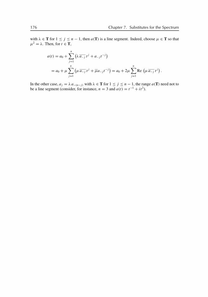
buch72005/10/5page 176

�

�

�

�

�

�

�

�


with λ ∈ T for 1 ≤ j ≤ n− 1, then a(T) is a line segment. Indeed, choose μ ∈ T so thatμ2 = λ. Then, for t ∈ T,

a(t) = a0 +n∑

j=1

(λ a−j t j + a−j t

−j)

= a0 + μ

n∑j=1

(μ a−j t j + μa−j t

−j) = a0 + 2μ

n∑j=1

Re(μ a−j t j

).

In the other case, aj = λ a−(n−j) with λ ∈ T for 1 ≤ j ≤ n− 1, the range a(T) need not tobe a line segment (consider, for instance, n = 3 and a(t) = t−1 + it2).

buch72005/10/5page 177

�

�

�

�

�

�

�

�

Chapter 8

Transient Behavior

Let An be a complex n × n matrix. The behavior of the norms ‖Akn‖ is of considerable

interest in connection with several problems. We specify ‖ · ‖ to be the spectral norm ‖ · ‖2.The norms ‖Ak

n‖2 converge to zero as k → ∞ if and only if rad An < 1, where rad An

denotes the spectral radius of An. However, sole knowledge of the spectral radius or evenof all the eigenvalues of An does not tell us whether the norms ‖Ak

n‖2 run through a criticaltransient phase, that is, whether there are k for which ‖Ak

n‖2 becomes very large, beforeeventually decaying exponentially to zero. In this chapter we embark on this problem in thecase where An is a Toeplitz band matrix.

8.1 The General MessageSo what can be said about the norms ‖T k

n (b)‖2 := ‖(Tn(b))k‖2? The computer is expectedto give a reliable answer in the case where n is small. We therefore assume that n is large.The message of this chapter is that ‖T k

n (b)‖2 has critical behavior as k increases (whichmeans that the norms ‖T k

n (b)‖2 become large before decaying to zero or that the norms‖T k

n (b)‖2 go to infinity) if and only if ‖b‖∞ > 1. In other words, to find out whether‖T k

n (b)‖2 shows critical transient or limiting behavior, we need only look whether the L∞norm of the symbol is greater than one. Notice that it is much more difficult to decidewhether rad Tn(b) or lim supn→∞ rad Tn(b) is smaller than one (see Sections 10.3 and 10.4).

Since Tn(b) = PnT (b)Pn|Im Pn, it follows at once that

‖T kn (b)‖2 ≤ ‖Tn(b)‖k

2 ≤ ‖T (b)‖k2 = ‖b‖k

∞ (8.1)

for all n and k. Thus, for the norms of powers of Toeplitz matrices we have the simpleuniversal upper estimate (8.1). In particular, if ‖b‖∞ ≤ 1, then there is no critical behavior.The following theorem shows that (8.1) contracts to an equality in the n →∞ limit. Thistheorem may be viewed as an argument in support of the statement that ‖T k

n (b)‖ showscritical behavior whenever ‖b‖∞ > 1.

177

buch72005/10/5page 178

�

�

�

�

�

�

�

�

178 Chapter 8. Transient Behavior

Theorem 8.1. If b ∈ W , then

limn→∞‖T

kn (b)‖2 = ‖b‖k

∞

for each natural number k.

Proof. This follows from Corollary 5.14. Here is a direct proof. For fixed k, the operatorsT k

n (b) converge strongly to T k(b) as n→∞. Hence, by the Banach-Steinhaus theorem,

lim infn→∞ ‖T k

n (b)‖2 ≥ ‖T k(b)‖2. (8.2)

By (8.1) and (8.2), we are left with proving that ‖T k(b)‖2 ≥ ‖b‖k∞. But ‖T k(b)‖2 ≥rad T k(b) = (rad T (b))k , and Corollary 1.12 says that the spectrum of T (b) contains therange of b, whence rad T (b) ≥ ‖b‖∞.

The problem studied here amounts to looking for peaks of the “surface” (k, n) �→‖T k

n (b)‖2 along the linesn = constant, whileTheorem 8.1 concerns the behavior of‖T kn (b)‖2

along the lines k = constant. We will return to this question later. For the moment, let usconsider an example.

Example 8.2. The simplest nontrivial Toeplitz matrix is the Jordan block

Jn(λ) =

⎛⎜⎜⎜⎜⎜⎝λ 0 0 . . . 01 λ 0 . . . 00 1 λ . . . 0...

......

. . ....

0 0 0 . . . λ

⎞⎟⎟⎟⎟⎟⎠ . (8.3)

Clearly, Jn(λ) = Tn(b) with b(t) = λ + t (t ∈ T). Figure 8.1 indicates the shape ofthe “surface” (k, n) �→ ‖J k

n (0.8)‖2. We will omit the quotation marks in the followingand will simply speak of the norm surface. We will also silently identify the surface withits “map” in the k, n plane; that is, we will not distinguish the point (k, n, f (k, n)) onthe surface from its projection (k, n) in the plane. The spectral radius of Jn(0.8) equals0.8, while the L∞ norm of the symbol is ‖b‖∞ = 1.8. We see that the surface has alowland (say below the curve ‖J k

n (0.8)‖2 = 10−6, a steep region (say between the curves‖J k

n (0.8)‖2 = 10−6 and ‖J kn (0.8)‖2 = 102), and a part where it grows enormously (say

above the curve ‖J kn (0.8)‖2 = 102). We call the last part the sky region. If n is fixed and k

increases, we move horizontally in Figure 8.1. On the surface, we will soon be in the skyregion, then step down the steep region, and finally be caught in the lowland forever. Thus,we have the critical transient phase shown in the left picture of Figure 8.2. On the otherhand, if we fix k and let n increase, then this corresponds to a vertical movement in Figure8.1. This time we will fairly quickly reach the sky region and move at nearly constant heightfor the rest of the journey, as shown the right picture of Figure 8.2. Note that in the rightpicture of Figure 8.2 the norms converge to the limit 1.820 = 12.75 · 104 and that the normsare already very close to this limit beginning with n between 20 and 40.

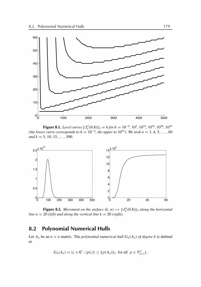
buch72005/10/5page 179

�

�

�

�

�

�

�

�

8.2. Polynomial Numerical Hulls 179

0 100 200 300 400 5000

10

20

30

40

50

60

Figure 8.1. Level curves ‖J kn (0.8)‖2 = h for h = 10−6, 102, 1010, 1018, 1026, 1034

(the lower curve corresponds to h = 10−6, the upper to 1034). We took n = 3, 4, 5, . . . , 60and k = 5, 10, 15, . . . , 500.

0 100 200 300 400 5000

0.5

1

1.5

2

2.5x 1012

0 20 40 600

2

4

6

8

10

12

14x 104

Figure 8.2. Movement on the surface (k, n) �→ ‖J kn (0.8)‖2 along the horizontal

line n = 20 (left) and along the vertical line k = 20 (right).

8.2 Polynomial Numerical HullsLet An be an n × n matrix. The polynomial numerical hull Gk(An) of degree k is definedas

Gk(An) = {z ∈ C : |p(z)| ≤ ‖p(An)‖2 for all p ∈ P+k+1},

buch72005/10/5page 180

�

�

�

�

�

�

�

�


where P+k+1 is the set of all polynomials of the form

p(z) = p0 + p1z+ · · · + pkzk.

The objective of Gk(An) is to employ the obvious inequality

‖p(An)‖2 ≥ maxz∈Gk(An)

|p(z)|

in order to get a lower estimate for ‖p(An)‖2. The sets Gk(An) were introduced by OlaviNevanlinna [192], [193] and were independently discovered by Anne Greenbaum [141],[142]. Their works describe various properties of polynomial numerical hulls. In general,polynomial numerical hulls can be computed only numerically (see, e.g., [141]), and thedevelopment of algorithms and software for polynomial numerical hulls is still far awayfrom the advanced level of the pseudospecta counterpart [299], [300].

Faber, Greenbaum, and Marshall [112] obtained remarkably precise results on thepolynomial numerical hulls of Jordan blocks. Let Jn(λ) be the Jordan block (8.3). If k

is greater than the degree of the minimal polynomial of An, then Gk(An) collapses to thespectrum of An. Thus, Gk(Jn(λ)) = {λ} for k ≥ n. In [112], it is shown that if 1 ≤ k ≤ n−1,then Gk(Jn(λ)) is a closed disk with the center λ whose radius �n,k satisfies

cosπ

n+ 1= �1,n ≥ �k,n ≥ �n−1,n = 1− log(2n)

n+ log(log(2n))

n+ o

(1

n

).

Consequently,

‖J kn (λ)‖2 ≥ max|ζ−λ|≤�n,k

|ζ |k = (|λ| + �n,k)k.

It is also shown in [112] that �n−1,n is greater than or equal to the positive root of 2rn+r−1 =0, which implies that

�n−1,n > 1− log(2n)

nfor all n.

This yields, for instance, ‖J 50100(0.8)‖2 ≥ 1012.11. MATLAB gives that ‖J 50

100(0.8)‖2 equals1012.76.

We remark that a matrix with a norm that is gigantic in comparison with the matrixdimension must have a gigantic entry. For n > k, the �th entry of the first column of thelower-triangular Toeplitz matrix J k

n (λ) is ( k� ) λk−�. Taking � = [k/(1 + |λ|)], where [·]

denotes the integer part, we get

‖J kn (λ)‖2 ≥

(k

[k/(1+ |λ|)])|λ|k−[k/(1+|λ|)].

This simple observation delivers

‖J 50100(0.8)‖2 ≥

(5027

)0.823 = 1011.80,

which is fairly good.

buch72005/10/5page 181

�

�

�

�

�

�

�

�

8.3. The Pseudospectra Perspective 181

8.3 The Pseudospectra PerspectiveThe role of pseudospectra in connection with the norms of powers of matrices and operators isas follows: norms of powers can be related to the resolvent norm, and pseudospectra decodeinformation about the resolvent norm in a visual manner. A relation between resolvent andpower norms is established by the Kreiss matrix theorem. Let An be an n× n matrix withrad An ≤ 1. For λ outside the closed unit disk D, put Rn(λ) = ‖(An−λI)−1‖2. The Kreissmatrix theorem says that

sup|λ|>1

(|λ| − 1)Rn(λ) ≤ maxk≥0

‖Akn‖2 ≤ en sup

|λ|>1(|λ| − 1)Rn(λ).

We refer the reader to [289] for a delightful discussion of the theorem. The “easy half” ofthe Kreiss matrix theorem is the lower estimate. It implies that if we pick a point λ ∈ C with� := |λ| > 1, then the maximum of the norms ‖Ak

n‖2 (k ≥ 0) is at least (�−1)Rn(λ). Thus,the maximum is seen to be large whenever we can find a λ outside D with large resolventnorm.

The following theorem and its proof are due to Nick Trefethen [272]. This theoremis similar to but nevertheless slightly different from the lower estimate of the Kreiss matrixtheorem.

Theorem 8.3. Let A be a bounded linear operator and let λ ∈ C \ sp A. Put � = |λ| andR(λ) = ‖(A− λI)−1‖2. If R(λ) > 1/�, then

max1≤j≤k

‖Aj‖2 ≥ �k

/(1+ �k − 1

� − 1

1

�R(λ)− 1

). (8.4)

Proof. Put Mk = max1≤j≤k ‖Aj‖2. By assumption, �R(λ) − 1 is positive, so the term inthe large brackets of (8.4) is at least 1 and the right-hand side of (8.4) is thus at most �k . If �

does not exceed the spectral radius of A, then (8.4) is accordingly trivial. We may thereforeassume that � is larger than the spectral radius of A. In this case we have

λ(λI − A)−1 = (I − λ−1A)−1 = I + (λ−1A)+ (λ−1A)2 + (λ−1A)3 + · · ·and the corresponding bound

�R(λ) ≤ 1+ �−1‖A‖2 + �−2‖A2‖2 + �−3‖A3‖2 + · · · . (8.5)

Let us take the case k = 2 for illustration. Clearly,

‖A‖2, ‖A2‖2 ≤ M2, ‖A3‖2, ‖A4‖2 ≤ M22 , ‖A5‖2, ‖A6‖2 ≤ M3

2 ,

and so on. Grouping the terms in (8.5) accordingly into pairs gives

�R(λ) ≤ 1+ (�−2M2)(1+ �)+ (�−2M2)2(1+ �)+ · · · .

If M2 ≥ �2, then (8.4) is true, so we may assume that �−2M2 < 1. In this case

�R(λ) ≤ 1+ �−2M2(1+ �)

1− �−2M2= 1+ � + 1

�2/M2 − 1.

buch72005/10/5page 182

�

�

�

�

�

�

�

�


For general k, we obtain similarly that �R(λ) is at most

1+ (�−kMk)(1+ · · · + �k−1)+ (�−kMk)2(1+ · · · + �k−1)+ · · ·

= 1+ 1+ � + · · · + �k−1

�k/Mk − 1,

that is,

�R(λ)− 1 ≤ �k − 1

� − 1

1

�k/Mk − 1.

It follows that

1

�R(λ)− 1≥ � − 1

�k − 1

(�k

Mk

− 1

),

which implies that

�k

Mk

− 1 ≤ �k − 1

� − 1

1

�R(λ)− 1.

This is (8.4).

Thus, if sp A is known to be a subset of the closed unit disk D and if there is an ε ≤ 1such that the pseudospectrum spεA contains points outside D, then, by (7.1), each pointλ ∈ spεA \ D yields an estimate

max1≤j≤k

‖Aj‖2 ≥ �k

/(1+ �k − 1

� − 1

1

�/ε − 1

)(8.6)

with � = |λ|. Different choices of λ give different values of the right-hand sides of (8.4)and (8.6), and we want these right-hand sides to be as large as possible. Tom Wright [299],[300] has implemented the search for an optimal λ in EigTool.

Recall that P denotes the set of all Laurent polynomials. Fix b ∈ P and considerTn(b). We put

Mk(n) = max1≤j≤k

‖T jn (b)‖2, M(n) = lim

k→∞Mk(n).

Clearly, M(n) = supk≥1 Mk(n); that is, M(n) is the height of the highest peak of ‖T kn (b)‖2

as k ranges over N. Thus, the powers of Tn(b) go to infinity if and only if M(n) = ∞ andthey have a critical transient behavior before decaying to zero if and only if M(n) is largebut finite. We assume that the plane Lebesgue measure of sp T (b) is nonzero. Equivalently,we assume that there exist points in the plane that are encircled by the (naturally oriented)curve b(T) with nonzero winding number. Suppose ‖b‖∞ > 1. Then there exist pointsλ ∈ C \ b(T) such that � = |λ| > 1 and the winding number of b about λ is nonzero. FromTheorem 4.1 we know that

Rn(λ) := ‖(Tn(b)− λI)−1‖2 = ‖T −1n (b − λ)‖2

buch72005/10/5page 183

�

�

�

�

�

�

�

�


increases at least exponentially, i.e., there exist positive constants C = C(b, λ) and β =β(b, λ) such that

Rn(λ) ≥ Ceβn (8.7)

for all n ≥ 1. Consequently, Rn(λ) > 1 for all sufficiently large n and we obtain fromTheorem 8.3 that

Mk(n) ≥ �k

/(1+ �k − 1

� − 1

1

�Rn(λ)− 1

),

and

M(n) ≥ (� − 1)(�Rn(λ)− 1). (8.8)

This in conjunction with (8.7) gives

M(n) ≥ (� − 1)(�Ceβn − 1), (8.9)

that is, there must be critical transient or limiting behavior of ‖T kn (b)‖2 for all n larger than

a moderately sized n0. We will now say something about the constants in (8.7) and (8.9).We denote by Pr (r ≥ 1) the set of all Laurent polynomials of degree at most r , that

is, the set of all functions of the form

b(t) =r∑

j=−r

bj tj . (8.10)

Let b ∈ Pr and suppose br �= 0. Assume ‖b‖∞ > 1 and choose λ as above. For the sake ofdefiniteness, let wind (b, λ) = −κ ≤ −1. We have

t r (b(t)− λ) = br

s∏i=1

(t − μi)

2r∏i=s+1

(t − δi)

with |μi | > 1 and |δi | < 1 (recall Section 1.4). It follows that

b(t)− λ = br t−κ

s∏i=1

(t − μi)

2r∏i=s+1

(1− δj

t

),

where κ = s − r (≥ 1). Put

d(t) =s∏

i=1

(t − μi)−1 =:

∞∑j=0

dj tj (t ∈ T), (8.11)

‖Pnd‖22 =

n−1∑j=0

|dj |2, ‖Qnd‖22 =

∞∑j=n

|dj |2. (8.12)

Theorem 8.4. For all n ≥ 1,

Rn(λ) ≥ ‖Pnd‖2

‖b − λ‖∞‖Qnd‖2.

buch72005/10/5page 184

�

�

�

�

�

�

�

�


Proof. Put c = b − λ. With the notation χk(t) = tk , we have c = χ−κc−c+, where

c−(t) =2r∏

i=s+1

(1− δi

t

), c+(t) = br

s∏i=1

(t − μi).

Define x(n) ∈ Cn and x ∈ �2 by x(n) = (d0, . . . , dn−1) and x = {d0, d1, . . . }. SinceT (c) = T (c−)T (χ−κ)T (c+), we obtain

Tn(c)x(n) = PnT (c−)T (χ−κ)T (c+)x(n). (8.13)

Because κ ≥ 1, we have PnT (c−)T (χ−κ)e0 = 0, where e0 = {1, 0, 0, . . . }. As T (c+)x =e0, it follows that PnT (c−)T (χ−κ)T (c+)x = 0. This equality and (8.13) give

Tn(c)x(n) = PnT (c−)T (χ−κ)T (c+)(x(n) − x) = PnT (c)(x(n) − x).

Taking into account that ‖x(n) − x‖2 = ‖Qnd‖2, we arrive at the estimate

‖Tn(c)x(n)‖2 ≤ ‖T (c)‖2 ‖Qbd‖2 = ‖c‖∞‖Qnd‖2,

and since ‖x(n)‖2 = ‖Pnd‖2, it results that

‖T −1n (c)‖2 ≥ ‖x(n)‖2

‖Tn(c)x(n)‖2≥ ‖Pnd‖2

‖c‖∞‖Qnd‖2.

For the sake of simplicity, assume that the zeros μ1, . . . , μs are distinct and that|μ1| < |μi | for all i ≥ 2. Decomposition into partial fractions gives

d(t) =s∑

i=1

Ai

1− t/μi

=∞∑

j=0

s∑i=1

Ai

μj

i

tj , (8.14)

with explicitly available constants A1, . . . , As . Theorem 8.4 in conjunction with the esti-mates

‖Pnd‖2 ≥ |d0| =∣∣∣∣∣

s∑i=1

Ai

∣∣∣∣∣ =s∏

i=1

1

|μi |and

‖Qnd‖22 =

∞∑j=n

∣∣∣∣∣s∑

i=1

Ai

μj

i

∣∣∣∣∣2

≤ s

s∑i=1

∞∑j=n

|Ai |2|μi |2j

=s∑

i=1

|Ai |2|μi |2n

s

1− 1/|μi |2

=:s∑

i=1

Bi

|μi |2n= B1

|μ1|2n

(1+

s∑i=2

Bi

B1

∣∣∣∣μ1

μi

∣∣∣∣2n)

yields

Rn(λ)2 ≥ |μ1|2n

B1‖b − λ‖2∞∏s

i=1 |μi |21

1+∑si=2(Bi/B1)|μ1/μi |2n

. (8.15)

buch72005/10/5page 185

�

�

�

�

�

�

�

�


In practice, we could try computing Rn(λ) directly via the MATLAB commandsRn(λ) = norm(inv(Tn(b − λ))) or Rn(λ) = 1/min(svd(Tn(b − λ))). However, as (8.7)shows, this is an ill-conditioned problem for large n. Estimate (8.15) is more reliable. Itfirst of all shows that (8.7) and (8.9) are true with

β = log |μ1|.To get the constants contained in (8.15) we may proceed as follows. We first determinethe zeros μ1, . . . , μs , we then use MATLAB’s residue command to find the numbers Ai

in formula (8.14), and finally we put Bi = s|Ai |2/(1 − 1/|μi |2). Note that s is in generalmuch smaller than n so that possible numerical instabilities are no longer caused by largematrix dimensions but at most by unfortunate location of the zeros μ1, . . . , μs . Notice alsothat (8.11) implies that the numbers d0, . . . , ds−1 are the entries of the first column of thelower-triangular Toeplitz matrix Ts(d). Thus, alternatively we could solve the s × s system

Ts

(s∏

i=1

(t − μi)

)( d0 . . . ds−1 )� = ( 1 0 . . . 0 )�

to obtain d0, . . . , ds−1 and then, taking into account (8.14), find the constants A1, . . . , As

as the solutions of the s × s Vandermonde system⎛⎜⎜⎜⎝1 1 . . . 1

1/μ1 1/μ2 . . . 1/μs

......

...

1/μs−11 1/μs−1

2 . . . 1/μs−1s

⎞⎟⎟⎟⎠⎛⎜⎜⎜⎝

A1

A2...

As

⎞⎟⎟⎟⎠ =

⎛⎜⎜⎜⎝d0

d1...

ds−1

⎞⎟⎟⎟⎠ .

Here is an example that can be done by hand.

Example 8.5. Let b(t) = t−1 + α2t with 0 < α < 1/2. The range b(T) is the ellipse

x2

(1+ α2)2+ y2

(1− α2)2= 1

and the eigenvalues of the matrix Tn(b) are densely spread over the interval (−2α, 2α)

between the foci of the ellipse. The spectral radius is

rad (Tn(b)) = 2α cosπ

n+ 1.

This is smaller than 1 but may be close to 1. The norm of the symbol is ‖b‖∞ = 1+α2 > 1.Fix λ = � ∈ (1, 1+ α2). The zeros of t (b(t)− �) are

μ1 = � −√�2 − 4α2

2α2, μ2 = � +√

�2 − 4α2

2α2.

The numbers μ1 and μ2 are greater than 1, and we have

A1 = 1

μ1 − μ2, A2 = 1

μ2 − μ1, B1 = 2A2

1

1− 1/μ21

, B2 = 2A22

1− 1/μ22

.

buch72005/10/5page 186

�

�

�

�

�

�

�

�


Thus, (8.15) becomes

Rn(λ)2 ≥ α4μ2n1

B1(� + 1+ α2)2

/(1+ B2

B1

(μ1

μ2

)2n)

.

Here are a few concrete samples. In each case we picked λ = � = 1.01. Note that (8.8)with � = 1.01 gives

M(n) ≥ 0.1(1.01 Rn(1.01)− 1),

which is almost the same as the Kreiss estimate M(n) ≥ 0.1Rn(1.01).

α = 0.2. We have μ1 = 1.0323, μ2 = 24.2177,

Rn(1.01) ≥ 100.0138 n−1.0863 =: E0.2(n).

In particular, E0.2(1000) = 1012.70. MATLAB result: R1000(1.01) = 1015.03.

α = 0.4. Now μ1 = 1.2296, μ2 = 5.0829,

Rn(1.01) ≥ 100.0897 n−0.9316 =: E0.4(n).

We get E0.4(100) = 108.04 and E0.4(1000) = 1088.77, while the MATLAB results areR100(1.01) = 109.48 and R1000(1.01) = 1090.28.

α = 0.49. This time μ1 = 1.5945, μ2 = 2.6121,

Rn(1.01) ≥ 100.2026 n−1.2233 =: E0.49(n).

We obtain

E0.49(50) = 108.91, E0.49(100) = 1019.04,

E0.49(1000) = 10201.38, E0.49(2000) = 10403.98,

and MATLAB delivers

R50(1.01) = 1010.22, R100(1.01) = 1020.35, R1000(1.01) = 10202.71;the last two values are delivered with a warning. MATLAB returns a warning without avalue for n = 2000.

8.4 A Triangular ExampleThe next question after Theorem 8.1 concerns the convergence speed. Let b ∈ P be of theform b(t) = ∑

j≥0 bj tj , that is, suppose T (b) is lower triangular. Assume also that |b| is

not constant on T. We have T kn (b) = Tn(b

k), and hence we may employ Theorem 5.8 withb replaced by bk . It results that there are constants ck, dk ∈ (0,∞) and γ ∈ {1, 2, . . . } suchthat

‖b‖k∞ −

dk

n2γ≤ ‖T k

n (b)‖2 ≤ ‖b‖k∞ −

ck

n2γ(8.16)

buch72005/10/5page 187

�

�

�

�

�

�

�

�

8.5. Gauss-Seidel for Large Toeplitz Matrices 187

for all n ≥ 1. However, the constants ck and dk may be large if k is large. We remark thatthe constants C of inequalities like

‖b‖∞ − |b(t)| ≤ C|t − t0|2γ (8.17)

enter the d2 of (5.14). For the powers of b, we obtain from (8.17) something like

‖b‖k∞ − |bk(t)| � Ck‖b‖k

∞|t − t0|2γ ,

and since Ck‖b‖k∞ is large whenever ‖b‖∞ > 1 and k is large, we can expect that dk is alsolarge.

Let us consider a concrete example. Take

b(t) = 10

(− 1

16− 1

4t + t2 − 1

4t3 − 1

16t4

)= 10t2

(11

8− 1

16|1− t |4

).

In this case 2γ = 4. The spectral radius of Tn(b) is about 0.63 and ‖b‖∞ equals 110/8 =13.75. The level curves of the norm surface are shown in Figure 8.3 and we clearly see theexpected critical transient behavior. An interesting feature of Figure 8.3 is the indents ofthe level curves. These indents correspond to vertical valleys in the surface. For instance,along the horizontal line n = 18 we have Figure 8.4. The interesting piece of Figure 8.4 isbetween k = 15 and k = 40. If we move vertically along one of the lines k = 15, k = 20,. . . , k = 40, we obtain Figure 8.5. Figure 8.6 reveals some mild turbulence in the steepregion, but Figure 8.5 convincingly shows that in the sky region everything goes smoothly.In particular, the speed of the convergence of ‖T k

n (b)‖2 to ‖T k(b)‖2 = ‖b‖k∞ is not affectedby small fluctuations of the exponent k.

8.5 Gauss-Seidel for Large Toeplitz MatricesTo solve the n × n system Cnx = y, one decomposes Cn into a sum Cn = Ln + Un ofa lower-triangular matrix Ln and an upper-triangular matrix Un with zeros on the maindiagonal. If Ln is invertible, then the system Cnx = y is equivalent to the system

x = −L−1n Unx + L−1

n y. (8.18)

The Gauss-Seidel iteration consists of choosing an initial x0 and computing the iterationsby

xk+1 = −L−1n Unxk + L−1

n y. (8.19)

Sometimes (8.18) and (8.19) are written in the form

x = x + L−1n (y − Cnx), xk+1 = xk + L−1

n (y − Cnxk).

We have xk − x = (−L−1n Un)

k(x0 − x). Thus, the iteration matrix is An := −L−1n Un =

I − L−1n Cn, and the iteration converges whenever rad An < 1. The problem is whether a

critical transient behavior of the norms ‖Akn‖ may garble the solution.

buch72005/10/5page 188

�

�

�

�

�

�

�

�


0 50 100 150 200 250 300 350 4000

5

10

15

20

25

30

35

40

Figure 8.3. The symbol is b(t) = 10 (− 116 − 1

4 t + t2 − 14 t3 − 1

16 t4). The plotshows the level curves ‖T k

n (b)‖2 = h for h = 10−2, 1, 102, 104, . . . , 1024 (the lowercurve corresponds to h = 10−2, the upper to 1024). We took 6 ≤ n ≤ 40 and k =10, 15, 20, . . . , 400.

0 20 40 60 80 1000

0.5

1

1.5

2

2.5

3x 10

12

Figure 8.4. The symbol is as in Figure 8.3. The picture shows the norms ‖T k18(b)‖2

for 1 ≤ k ≤ 100.

buch72005/10/5page 189

�

�

�

�

�

�

�

�


0 10 20 30 40 50 60 700

5

10

15

20

25

30

35

40

45

Figure 8.5. The symbol is again as in Figure 8.3. We see the values oflog10 ‖T k

n (b)‖2 for 6 ≤ n ≤ 70 and k = 15, 20, 25, . . . , 40. Eventually higher curvescorrespond to higher values of k.

6 8 10 12 14 16 18

2

4

6

8

10

12

Figure 8.6. A close-up of Figure 8.5.

buch72005/10/5page 190

�

�

�

�

�

�

�

�


Now suppose Cn = Tn(c) is a Toeplitz matrix and let us for the sake of simplicityassume that

c(t) =∞∑

j=−∞cj t

j , where∞∑

j=−∞|cj | <∞.

We write Cn = Ln + Un = Tn(c+)+ Tn(c−) with

c+(t) =∞∑

j=0

cj tj , c−(t) =

−1∑j=−∞

cj tj .

If c+(z) �= 0 for |z| ≤ 1, then the inverse of Tn(c+) is Tn(c−1+ ) and the iteration matrix

becomes An = −Tn(c−1+ )Tn(c−). The spectrum of An is the set of all complex numbers λ

for which

−Tn(c−1+ )Tn(c−)− λI = −Tn(c

−1+ )Tn(c− + λc+)

is not invertible. Since Tn(c−1+ ) is invertible by assumption, we have to look for the λ’s for

which Tn(c− + λc+) is not invertible.By the Banach-Steinhaus theorem,

lim infn→∞ ‖Ak

n‖2 = lim infn→∞ ‖(Tn(c

−1+ )Tn(c−))k‖2 ≥ ‖(T (c−1

+ )T (c−))k‖2.

Propositions 1.2 and 1.3 imply that (T (c−1+ )T (c−))k is T (c−k

+ ck−) plus a compact operator.The function c−k

+ ck− is not a Laurent polynomial, but it lies in the Wiener algebra, and theargument of the proof of Lemma 5.12 remains valid for symbols in the Wiener algebra. Thisshows that ‖(T (c−1

+ )T (c−))k‖2 ≥ ‖c−k+ ck−‖∞ = ‖c−1

+ c−‖k∞. Consequently,

lim infn→∞ ‖Ak

n‖2 ≥ ‖c−1+ c−‖k

∞. (8.20)

Thus, if n is large enough, a critical transient phase will certainly occur in the case where‖c−1+ c−‖∞ > 1.

If a(t) = a−1t−1 + a0 + a1t , then the eigenvalues of Tn(a) are known to be

a0 + 2√

a1a−1 cosπj

n+ 1(j = 1, . . . , n)

(Theorem 2.4). Hence, in case c is a trinomial, c(t) = c−1t−1 + c0 + c1t , the matrix

Tn(c− + λc+) has the eigenvalues

λc0 + 2√

c1c−1

√λ cos

πj

n+ 1(j = 1, . . . , n).

It follows that

sp An ={

4c1c−1

c20

cos2 πj

n+ 1: j = 1, . . . , n

}

buch72005/10/5page 191

�

�

�

�

�

�

�

�


and

rad An = 4|c1| |c−1||c0|2 cos2 π

n+ 1.

Anne Greenbaum [141] discussed the example c(t) = −1.16t−1 + 1 + 0.16t . Thespectral radius of An is about 0.73. Using (numerically computed) polynomial numericalhulls, she obtained that ‖A29

30‖2 ≥ 1.25629 ≈ 700 and trying the computer directly, shearrived at the much better result ‖A29

30‖2 ≈ 104. Our estimate (8.20) with c+(t) = 1+ 0.16t

and c−(t) = −1.16t−1 gives

lim infn→∞ ‖A29

n ‖2 ≥ ‖c−1+ c−‖29

∞ = maxt∈T

∣∣∣∣−1.16t−1

1+ 0.16t

∣∣∣∣29

=(

1.16

1− 0.16

)29

= 1.38129 = 104.07. (8.21)

Thus, although (8.21) is an “n → ∞” result, it is already strikingly good for n about 30.Figure 8.7 shows the norm surface.

0 50 100 1500

5

10

15

20

25

30

35

40

45

50

Figure 8.7. The norm surface for An = Tn(c−1+ )Tn(c−) with c+(t) = 1 + 0.16t

and c−(t) = −1.16t−1. The picture shows the level curves ‖Akn‖2 = h for h = 10−2, 1, 102,

104, 106 (the lower curve corresponds to h = 10−2, the upper to 106). We took 3 ≤ n ≤ 50and k = 5, 10, 15, . . . , 150.

Nick Trefethen [270] considered the symbol c(t) = t−1 − 2+ t . In this case c+(t) =−2+ t and c−(t) = t−1, so

‖c−1+ c−‖∞ = max

t∈T

∣∣∣∣ t−1

−2+ t

∣∣∣∣ = 1,

buch72005/10/5page 192

�

�

�

�

�

�

�

�


and hence (8.20) does not provide any useful piece of information. However, the bruteestimate

‖Akn‖2 ≤ ‖Tn(c

−1+ )‖k

2‖Tn(c−)‖k2 ≤ ‖c−1

+ ‖k∞‖c−‖k

∞ = maxt∈T

∣∣∣∣ 1

−2+ t

∣∣∣∣k· 1k = 1

shows that there is no critical behavior. The spectral radius of An is cos2 πn+1 , which is

approximately 0.9990325 for n = 100. MATLAB gives rad A100 = 0.9990 (fantastic!) andtells us that the norms ‖Ak

100‖2 are 0.9080, 0.6169, and 0.3804 for k = 100, 500, 1000,respectively.

8.6 Genuinely Finite ResultsWe begin with an observation similar to Proposition 5.11. We denote by Pr the set of allLaurent polynomials of the form

∑rj=−r bj t

j .

Lemma 8.6. Let b ∈ Pr and n > 2r(k − 1). Then

T kn (b) = Tn(b

k)+ PnXkPn +WnYkWn

with r(k − 1)× r(k − 1) matrices Xk and Yk independent of n.

Proof. For k = 1, the assertion is true with X1 = Y1 = 0. Assume the assertedequality is valid for k. We prove it for k + 1. Obviously,

T k+1n (b) = Tn(b

k)Tn(b)+ PnXkPnT (b)Pn +WnYkWnPnT (b)Pn.

By Proposition 3.10,

Tn(bk)Tn(b) = Tn(b

k+1)− PnH(bk)H (b)Pn −WnH(bk)H(b)Wn.

We have

H(bk) =

⎛⎜⎜⎜⎜⎜⎝Z11 . . . Z1k 0 . . ....

......

Zk1 . . . Zkk 0 . . .

0 . . . 0 0 . . .

. . . . . . . . . . . . . . .

⎞⎟⎟⎟⎟⎟⎠ , H (b) =⎛⎝ U 0 . . .

0 0 . . .

. . . . . . . . .

⎞⎠

with certain r × r blocks Zij and U , which implies that

H(bk)H (b) =

⎛⎜⎜⎜⎜⎜⎝Z11U 0 . . .

......

Zk1U 0 . . .

0 0 . . .

. . . . . . . . .

⎞⎟⎟⎟⎟⎟⎠ .

buch72005/10/5page 193

�

�

�

�

�

�

�

�

8.6. Genuinely Finite Results 193

Thus, PnH(bk)H (b)Pn = PnX′k+1Pn with a kr × r matrix X′

k+1 independent of n. Analo-gously, WnH(bk)H(b)Wn = WnY

′k+1Wn with some kr × r matrix Y ′k+1. Further,

Xk =

⎛⎜⎜⎜⎜⎜⎝X11 . . . X1,k−1 0 . . ....

......

Xk−1,1 . . . Xk−1,k−1 0 . . .

0 . . . 0 0 . . .

. . . . . . . . . . . . . . .

⎞⎟⎟⎟⎟⎟⎠and

T (b) =

⎛⎜⎜⎝A0 A−1

A1 A0 A−1

A1 A0 A−1

. . . . . . . . .

⎞⎟⎟⎠with r × r blocks Xij and A� independent of n. This shows that at most the first (k − 1)r

rows of XkPnT (b) are nonzero. For 1 ≤ j ≤ k − 1 and � ≥ k + 1, the j, � block ofXkPnT (b) is

k−1∑m=1

XjmAm−� = Xj,�−1A−1 +Xj,�A0 +Xj,�+1A1,

and as Xj,�−1 = Xj,� = Xj,�+1 = 0 for � ≥ k+1, it follows that at most the first kr columnsof XkPnT (b) are nonzero. Thus, PnXkPnT (b)Pn = PnX

′′k+1Pn with some (k − 1)r × kr

matrix X′′k+1 independent of n. Finally,

WnYkWnPnT (b)Pn = WnYkPnT (b)Wn,

and the same argument as above shows that this equals WnY′′k+1Wn with some (k− 1)r× kr

matrix Y ′′k+1 that does not depend on n.

Inequality (8.16) is an asymptotic result. In contrast to this, Corollary 5.19 is genuinelyfinite. Combining Lemma 8.6 and Corollary 5.19 with M2 = M0

2 = ‖b‖k∞ yields theinequality

‖b‖k∞

(1− 41r(k − 1)

n

)≤ ‖T k

n (b)‖2 ≤ ‖b‖k∞ (8.22)

for all n and k. Unfortunately, the lower bound of (8.22) is positive for n > 41r(k − 1)

only, which is not yet of much use for n’s below 1000. Better estimates can be derivedfrom Theorem 5.10 on the Fejér means. Here is such an estimate. It is already applicableto n > 2r(k − 1).

Theorem 8.7. If b ∈ Pr and n > 2r(k − 1), then ‖T kn (b)‖2 ≥ ‖σn−2r(k−1)(b

k)‖∞.

Proof. By Lemma 8.6,

T kn (b) = Tn(b

k)+⎛⎝ Xk 0 0

0 0 00 0 WkYkWk

⎞⎠ =⎛⎝ ∗ ∗ ∗∗ A ∗∗ ∗ ∗

⎞⎠ ,

buch72005/10/5page 194

�

�

�

�

�

�

�

�


where Xk and WkYkWk are (k − 1)r × (k − 1)r matrices and A = Tn−2r(k−1)(bk). This

implies that

‖T kn (b)‖2 ≥ ‖A‖2 = ‖Tn−2r(k−1)(b

k)‖2.

It remains to combine the last inequality and Theorem 5.10.

Recall that ‖ · ‖W is the Wiener norm of a Laurent polynomial: ‖b‖W =∑j |bj |.

Theorem 8.8. If b ∈ Pr and n > r(3k − 2), then

‖T kn (b)‖2 ≥ ‖b‖k

∞ −kr

n− 2r(k − 1)‖b‖k

W .

Proof. For a ∈ Pkr and m = n− 2r(k − 1) > kr ,

(σma)(t) =∑|j |≤kr

(1− |j |

m

)aj t

j =∑|j |≤kr

aj tj − 1

m

∑|j |≤kr

|j |aj tj ,

whence

|(σma)(t)| ≥∣∣∣∣∣∣∑|j |≤kr

aj tj

∣∣∣∣∣∣− kr

m

∑|j |≤kr

|aj |

and thus ‖σma‖∞ ≥ ‖a‖∞ − (kr/m)‖a‖W . This inequality in conjunction with Theorem8.7 gives the assertion.

Corollary 8.9. If b ∈ Pr and bj ≥ 0 for all j , then

‖T kn (b)‖2 ≥ n− 3kr

n− 2kr

⎛⎝∑j

bj

⎞⎠k

for n ≥ 3kr.

Proof. In this case ‖b‖∞ = ‖b‖W =∑j bj and, hence, by Theorem 8.8,

‖T kn (b)‖2 ≥

(1− kr

n− 2r(k − 1)

)(∑bj

)k ≥ n− 3kr

n− 2kr

(∑bj

)k

.

Example 8.10. Let b(t) = t + α2t−1 with α ∈ R. From Corollary 8.9 we infer that

1

2(1+ α2)k ≤ ‖T k

4k(b)‖2 ≤ (1+ α2)k

for all k ≥ 1.

Example 8.11. Suppose T (b) is lower triangular. Then T kn (b) = Tn(b

k) for all n and k, andhence we can have immediate recourse to Theorem 5.10 to obtain that

‖σn(bk)‖∞ ≤ ‖T k

n (b)‖2 ≤ ‖b‖k∞ for all n and k. (8.23)

buch72005/10/5page 195

�

�

�

�

�

�

�

�

8.7. The Sky Region Contains an Angle 195

Let first b(t) = λ+ t . Thus, Tn(b) is the Jordan block Jn(λ). For k ≤ n,

(σn(bk))(t) =

k∑j=0

(1− j

n

)(k

j

)λk−j t j = (λ+ t)k

(1− k

n

t

t + λ

)

and hence (8.23) yields(1− k

n

1

1+ |λ|)

(1+ |λ|)k ≤ ‖J kn (λ)‖2 ≤ (1+ |λ|)k (k ≤ n).

In particular,

1012.62 ≤ ‖J 50100(0.8)‖ ≤ 1012.77, 1025.17 ≤ ‖J 100

100 (0.8)‖ ≤ 1025.53,

which is better than the results of Section 8.1.Now let a(t) = t + t2. Then Tn(a) is a “super Jordan block” [270]. For every natural

number k,

‖σ2k(ak)‖∞ =

2k−1∑j=k

(1− j

2k

)(k

k − j

)= 3

82k,

and thus (8.23) implies that (3/8) 2k ≤ ‖T k2k(a)‖ ≤ 2k .

8.7 The Sky Region Contains an AngleLet b ∈ Pr and suppose ‖b‖∞ > 1. In Figures 8.1 and 8.3, the sky region looks approxi-mately like an angle: It is bounded by a nearly vertical line on the left and by a curve closeto the graph of a linear function n = ck + d from the right and below. The question iswhether this remains true beyond the cutouts we see in the pictures and whether this is validin general. To be more precise, we fix a (large) number B and we call the set

SB = {(k, n) : ‖T kn (b)‖2 > B}

the sky region (for our choice of the bound B). The following theorem proves that thelower-right boundary of the sky region is always linear or sublinear.

Theorem 8.12. If b ∈ Pr and ‖b‖∞ > 1, then there exist positive constants c and k0,depending on b and B, such that SB contains the angle {(k, n) : k > k0, n > ck}.

Proof. This is a simple consequence of inequality (8.22), which shows that

‖T kn (b)‖2 ≥ ‖b‖k

∞

(1− 41rk

n

)(8.24)

for all k and n: if k > k0 where ‖b‖k0∞ > 2B and n > 82rk, then the right-hand side of(8.24) is greater than B.

buch72005/10/5page 196

�

�

�

�

�

�

�

�


Thus, if we walk on the norm surface (k, n) �→ ‖T kn (b)‖2 along a curve whose

projection in the k, n plane is given by n = ϕ(k), then we will eventually reach any heightB and stay above this height forever provided ϕ(k)/k →∞. Note that this is satisfied forϕ(k) = k log log k. Or in yet other terms, if ϕ(k)/k →∞, then ‖T k

ϕ(k)(b)‖2 →∞.Theorem 8.12 is the deciding argument in support of the statement that ‖T k

n (b)‖2 runsthrough a critical transient phase if limn→∞ rad Tn(b) < 1 but ‖b‖∞ > 1. Suppose, forexample, k = 100. If the sky region were roughly of the form SB = {(k, n) : k > k0,n > k2}, then ‖T 100

n (b)‖2 would be larger than B for n > 10000 only. It is the linearityor sublinearity of the lower-right border of the sky region that allows us to conclude that‖T 100

n (b)‖2 is already larger than B for n in the hundreds.We call the number

LB(n) = #{k : ‖T kn (b)‖2 > B}

the length of the critical transient phase for the matrix dimension n. Theorem 8.12 impliesthat LB(n) > n/c − k0. In other words, LB(n) increases at least linearly with the matrixdimension n. Equivalently and a little more elegantly,

lim infn→∞

LB(n)

n> 0.

May the lower-right boundary of the sky region be strictly sublinear? Or alternatively,may the lowland contain an angle? Let b ∈ Pr and b(t) = ∑r

j=−r bj tj . For � ∈ (0,∞),

we define b� ∈ Pr by

b�(t) =r∑

j=−r

bj�j tj .

Theorem 8.13. Let b ∈ Pr , ‖b‖∞ > 1, and B > 1. If there exists a number � in (0,∞)

such that ‖b�‖∞ < 1, then SB is contained in an angle {(k, n) : n > ck + d} with c > 0and d > 0.

Proof. The key observation is due to Schmidt and Spitzer [243] and will be extensivelyexploited in Chapter 11. It consists of the equality Tn(b) = D−1

� Tn(b�) D�, where D� =diag (1, �, . . . , �n−1). Letting M = max(�, 1/�), we get

‖T kn (b)‖2 ≤ ‖D−1

� T kn (b�)D�‖2 ≤ ‖D−1

� ‖2 ‖T kn (b)‖2 ‖D�‖2 ≤ Mn−1‖b�‖k

∞

for all n and k. Thus, if (k, n) ∈ SB , then B < Mn−1‖b�‖k∞. Since � �= 1 and thus M > 1,it follows that

n > klog(1/‖b�‖∞)

log M+ log B

log M+ 1 =: ck + d,

and as ‖b�‖∞ < 1 and B > 1, we see that c > 0 and d > 0.

We will see in Chapter 10 that always

lim supn→∞

rad Tn(b) ≤ inf�∈(0,∞)

‖b�‖∞

buch72005/10/5page 197

�

�

�

�

�

�

�

�


and that in certain special cases the equality

limn→∞ rad Tn(b) = inf

�∈(0,∞)‖b�‖∞ (8.25)

holds. Equality (8.25) is particularly true if T (b) is Hermitian or tridiagonal or triangularor nonnegative, where nonnegativity means that bj ≥ 0 for all j . Hermitian matricesare uninteresting in our context, because for them the value given by (8.25) coincides with‖a‖∞. However, if T (b) is tridiagonal or triangular or nonnegative and if lim rad Tn(b) < 1,then (8.25) implies that we can find a � ∈ (0,∞) such that ‖b�‖∞ < 1 and hence, byTheorem 8.13, the sky region is contained in an angle. Equivalently, the lowland containsan angle. It also follows that in these cases

lim supn→∞

LB(n)

n<∞.

Suppose now that b ∈ Pr , lim rad Tn(b) < 1, and ‖b‖∞ > 1. If the lower borderof the sky region is strictly sublinear, then, by Theorem 8.13, inf ‖b�‖∞ must be at least1. We looked for such symbols in P3 and observed that they are difficult to identify. Thedetermination of inf ‖b�‖∞ for a given b ∈ P3 is simple. The problem comes with checkingwhether lim sup rad Tn(b) is smaller than 1 for a given candidate b ∈ P3. It turns out thatinf ‖b�‖∞ and lim sup rad Tn(b) are usually extremely close. We took 3000 random symbolsb ∈ P3 whose real and imaginary parts of the 7 coefficients b−3, . . . , b3 were drawn fromthe uniform distribution on (−1, 1). Each time MATLAB computed

q = inf�∈(0,∞)

‖b�‖∞/rad T64(b).

The result was as follows:

1.00 ≤ q < 1.02 in 2793 samples (= 93.1 %)

1.02 ≤ q < 1.04 in 117 samples (= 3.9 %)

1.04 ≤ q < 1.06 in 48 samples (= 1.6 %)

1.06 ≤ q < 1.08 in 23 samples (= 0.77 %)

1.08 ≤ q < 1.10 in 10 samples (= 0.33 %)

1.10 ≤ q < 1.20 in 9 samples (= 0.3 %)

and there was no sample with q ≥ 1.20. Thus, the dice show that if rad T64(b) ≤ 0.98,then inf ‖b�‖∞ is at most 1.02 · 0.98 = 0.9996 < 1 with probability about 93 % and ifrad T64(b) ≤ 0.83, then inf ‖b�‖∞ does not exceed 1.20 · 0.83 = 0.996 < 1 nearly surely.This result reveals that if we had a symbol b ∈ P3 for which lim sup rad Tn(b) < 1 andinf ‖b�‖∞ ≥ 1, then lim sup rad Tn(b) would be dramatically close to 1. Ensuring thatlim sup rad Tn(b) is really strictly smaller than 1 and guaranteeing at the same time thatinf ‖b�‖∞ ≥ 1 requires subtle tiny adjustments in the higher decimals after the comma ofthe coefficients. As we were not sure whether these subtleties survive the numerics neededplot the norm surface, that is, to compute ‖T k

n (b)‖2 for n in the 30’s and k in the hundreds,we gave up. Thus, we do not know a single symbol with strictly sublinear lower-right borderof the sky region or, equivalently, with a lowland that does not contain an angle.

buch72005/10/5page 198

�

�

�

�

�

�

�

�


Example 8.14. Figure 8.8 shows the norm surface for the symbol b(t) = t−1 + 0.492t .The spectral radius of Tn(b) is exactly 0.98 cos π

n+1 and ‖b‖∞ = 1+ 0.492 = 1.2401. Weclearly see the critical transient behavior of ‖T k

n (b)‖2 for n exceeding 20 or 30. We alsonicely see the indents in the level curves. The matrix T (b) is nonnegative, and hence, byTheorem 8.13, the sky region must be contained in an angle. The strange thing with Figure8.8 is that the lower-right pieces of the level curves nevertheless look slightly sublinear.Let n = ϕB(k) be the equation of the lower-right piece of the level curve ‖T k

n (b)‖2 = B.If ϕB were sublinear, then ϕB(k)/k would approach zero as k → ∞. The left picture ofFigure 8.9, showing 10 ϕB(k)/k and 10 ϕB(k) log k/k for 100 ≤ k ≤ 1000 does not yetconvincingly indicate that ϕB(k)/k tends to a positive finite limit. However, the right pictureof Figure 8.9, where we extended the range of the k’s up to 3000, reveals that there must bea positive finite limit for the lower curve 10 ϕB(k)/k.

Theorem 8.12 tells us that the lower-right boundary of the sky region is always sub-linear and Theorem 8.13 shows that it is superlinear in many cases. Things are completelydifferent for the n× n truncations An of arbitrary bounded linear operators on �2.

Let ψ : N → (e,∞) be any function such that ψ(n)→∞ as n→∞. We put

ξ(n) = ψ(n)

log ψ(n), λn = e−1/ξ(n).

Clearly, 1/e < λn < 1. We define the operator A by

A = diag (J2(λ1), J2(λ2), . . . )

:= diag

((λ1 01 λ1

),

(λ2 01 λ2

), . . .

).

Since λn < 1 for all n, the operator A is bounded on �2. We have

Akn =

{diag (J k

2 (λ1), . . . , Jk2 (λm)) for n = 2m,

diag (J k2 (λ1), . . . , J

k2 (λm), λk

m+1) for n = 2m+ 1.

The equality

J k2 (λ) =

(λk 0

kλk−1 λk

)and the condition 1/e < λ < 1 imply that

kλk ≤ kλk−1 ≤ ‖J k2 (λ)‖2 ≤ λk + kλk−1 ≤ (1+ ek)λk.

Consequently, up to constants independent of n and k, we may replace ‖Akn‖2 by kλk

m withm = [n/2]. The function fm(x) := xλx

m has its maximum at ξ(m) and fm(ξ(m)) =(1/e)ξ(m). If k ≥ ψ(m), then fm(k) ≤ fm(ψ(m)) because fm is monotonically decreasingon the right of ψ(m) (note that ψ(m) ≥ ξ(m)). As fm(ψ(m)) = 1, it follows that

SB ⊂ {(k, n) : k < ψ([n/2])} (8.26)

once B is large enough, say B > 10. Thus, on choosing very slowly increasing functionsψ , we obtain very narrow sky regions. In particular, the sky regions need not contain anyangles.

buch72005/10/5page 199

�

�

�

�

�

�

�

�


0 50 100 150 200 250 300 350 4000

5

10

15

20

25

30

35

40

Figure 8.8. The symbol is b(t) = t−1+ 0.492t . The picture shows the level curves‖T k

n (b)‖2 = h for h = 1, 10, 102, 103, . . . , 106 (the lower curve corresponds to h = 1, theupper to 106). We took 3 ≤ n ≤ 40 and k = 5, 10, 15, . . . , 400.

0 200 400 600 800 10000

0.5

1

1.5

2

2.5

3

0 1000 2000 30000

0.5

1

1.5

2

2.5

3

Figure 8.9. The symbol is b(t) = t−1 + 0.492t . The pictures show 10 ϕB(k)/k

and 10 ϕB(k) log k/k for B = 10−5 over two different ranges of k.

buch72005/10/5page 200

�

�

�

�

�

�

�

�


This is the right moment to return to what was said after Theorem 8.12. For theoperator A just constructed, we have ‖Ak

n‖2 � kλk[n/2] → k as n → ∞. Thus, when

moving along the line k = 104 on the norm surface, we will eventually be at a height ofabout 104 and may conclude that ‖Ak

n‖2 is close to 104 for all sufficiently large n. But if,for example, ψ(n) = log n for large n, then (8.26) shows that we will be in S104/2 onlyfor the n’s satisfying log[n/2] > k = 104, that is, for n > 2 exp(104) ≈ 2 · 104343. Webeautifully see that in this case movement along the lines k = constant does practically notprovide us with information about the evolution of the norms along the lines n = constant.Moral: Theorem 8.1 is a good reason for expecting critical behavior whenever ‖a‖∞ > 1,but it is Theorem 8.1 in conjunction with Theorem 8.12 that justifies this expectation withinreasonable dimensions.

In the language of critical transient phase lengths, (8.26) says that

lim supn→∞

LB(n)

ψ([n/2]) <∞

for the operator constructed above. An estimate in the reverse direction is also easy. Namely,it is readily seen that

fm

(1

2ξ(m)

)= 1

2√

eξ(m), fm(2 ξ(m)) = 2

2e2ξ(m),

and since 2/e2 < 1/(2√

e ), this shows that fm(k) > 2e2 ξ(m) for 1

2 ξ(m) < k < 2 ξ(m).Consequently, LB(n) ≥ (3/2)ξ([n/2]) if only (2/e2)ξ([n/2]) > B. As the last inequalityis satisfied for all sufficiently large n, we arrive at the conclusion that

lim infn→∞

LB(n)

ξ([n/2]) ≥3

2.

Finally, since ξ(m) = ψ(m)/ log ψ(m), it follows that

lim infn→∞

LB(n)

ψ([n/2]) log ψ([n/2]) > 0.

Rapidly growing functions ψ , such as ψ(n) = en, therefore yield gigantic critical phaselengths.

8.8 OscillationsLet b(t) = t−1 + 0.492t be as in Example 8.14. When plotting ‖T k

30(b)‖ for k between 1and 300, we see Figure 8.10 on the screen, and the purpose of this section is to explain theoscillating behavior in Figure 8.10.

Let An be an n×n matrix and suppose rad An < 1. For the sake of simplicity, assumethat all eigenvalues λ1, . . . , λn of An are simple. We then have An = C�C−1, where� = diag (λ1, . . . , λn) and C is an invertible n× n matrix. It follows that Ak

n = C�kC−1,and hence

Akn = C1λ

k1 + · · · + Cnλ

kn (8.27)

buch72005/10/5page 201

�

�

�

�

�

�

�

�

8.8. Oscillations 201

0 50 100 150 200 250 3000

1

2

3

4

5

6x 10

4

Figure 8.10. The symbol is b(t) = t−1 + 0.492t . We see the norms ‖T k30(b)‖2 for

k = 1, 2, 3, . . . , 300. A close-up is in the left picture of Figure 8.11.

with certain n× n matrices C1, . . . , Cn that do not depend on k (note that Cj is simply theproduct of the j th column of C by the j th row of C−1).

Assume that

|λ1| = · · · = |λs | > maxj≥s+1

|λj |.

Then (8.27) gives

Akn = C1λ

k1 + · · · + Csλ

ks +O(σk) as k →∞

with σ = maxj≥s+1 |λj |. Thus, if k is large, then

‖Akn‖2 ≈ ‖C1λ

k1 + · · · + Csλ

ks‖2, (8.28)

which has good chances for oscillatory behavior due to the fact that λ1 to λs have equalmoduli.

In the case where An is the Toeplitz matrix Tn(b) with b(t) = t−1+α2t , the eigenvaluesare given by

2α cosπj

n+ 1(j = 1, . . . , n).

buch72005/10/5page 202

�

�

�

�

�

�

�

�


The two dominating eigenvalues are

λ1 = 2α cosπ

n+ 1and λ2 = 2α cos

nπ

n+ 1= −2α cos

π

n+ 1.

Consequently,

‖T kn (b)‖2 ≈

(|2α| cos

π

n+ 1

)k

‖C1 + (−1)kC2‖2 (8.29)

for large k. Thus, the damping factor |2α|k cosk πn+1 has an amplitude that equals ‖C1+C2‖2

for even k and ‖C1 − C2‖2 for odd k. If the damping factor is not too small, then (8.29)(which holds for large k only) should be already valid in the critical transient phase so thatwe can see it with our eyes. This would be an explanation for the oscillating behavior inFigure 8.10. Let us check our example. Thus, take α = 0.49 and n = 30. Then

‖T 10030 (b)‖2 = 104.6457,

(0.98 cos

π

31

)100 ‖C1 + C2‖2 = 105.1438,

‖T 10130 (b)‖2 = 104.7014,

(0.98 cos

π

31

)101 ‖C1 − C2‖2 = 105.1959,

that is, (8.29) cannot be said to be satisfied. The point is that the modulus of the quotientof the dominant eigenvalues and the next eigenvalue is very close to 1, which impliesthat approximation (8.29) is not yet good enough in the high transient phase. However,consideration of a few more terms does set things right:

(0.98 cos

π

31

)k

∥∥∥∥∥C1 + (−1)kC2 + (C3 + (−1)kC4)

(cos(2π/31)

cos(π/31)

)k∥∥∥∥∥

2

equals 104.4597 and 104.5201 for k = 100 and k = 101, respectively, and

(0.98 cos

π

31

)k∥∥∥∥C1 + (−1)kC2 + (C3 + (−1)kC4)

(cos(2π/31)

cos(π/31)

)k

+ (C5 + (−1)kC6)

(cos(3π/31)

cos(π/31)

)k∥∥∥∥2

is 104.6512 and 104.7067 for k = 100 and k = 101, respectively.From the paper [96] by Brian Davies, we learned that such oscillation phenomena for

semigroup norms are well known. We also learned from [96] that the kind of oscillation maydepend on the norm chosen. Figures 8.11 and 8.12 show the different oscillatory behaviorof the spectral norms ‖T k

n (a)‖2 and the Frobenius norms ‖T kn (a)‖F fairly convincingly.

Finally, Figure 8.13 illustrates what happens when walking on the norm surface along thelines n = constant.

buch72005/10/5page 203

�

�

�

�

�

�

�

�

8.8. Oscillations 203

80 90 100 110 120

4.4

4.6

4.8

5

x 104

80 90 100 110 120

4.5

5

5.5

6

6.5x 10

4

Figure 8.11. The symbol is given by b(t) = t−1 + 0.492t . The left picture is aclose-up of part of Figure 8.10. The right picture shows the Frobenius norms ‖T k

30(b)‖F.

0 20 40 60 80 1000

2

4

6

8

10

12

14

16

18

Figure 8.12. The symbol is b(t) = t−1 + 0.492t . We see the norms ‖T k12(b)‖2

(lower curve) and the Frobenius norms ‖T k12(b)‖F (upper curve) for k = 1, 2, 3, . . . , 100.

buch72005/10/5page 204

�

�

�

�

�

�

�

�


0 50 100 150 2000

0.5

1

1.5

2

2.5

3x 109

32 34 36 380

1

2

3

4x 106

Figure 8.13. The symbol is again as in Figure 8.10. The pictures show the norms‖T 100

n (a)‖ (solid) and ‖T 101n (a)‖ (dashed) for two different ranges of n.

Another example is considered in Figures 8.14 and 8.15. Now the symbol is b(t) =1019 (t + t−2). We have rad T30(b) = 0.9847 and ‖b‖∞ = 1.04. The dominating eigenvaluesof T30(b) are

λ1 = μ, λ2 = μω, λ3 = μω2 (μ = 0.9847, ω = e2πi/3)

and hence

‖T k30(b)‖2 ≈

⎧⎨⎩‖C1 + C2 + C3‖2 |μ|k for k ≡ 0 (mod 3),

‖C1 + C2ω + C3ω2‖2 |μ|k for k ≡ 1 (mod 3),

‖C1 + C2ω2 + C3ω‖2 |μ|k for k ≡ 2 (mod 3).

The period 3 is nicely seen in the right picture of Figure 8.15.

8.9 ExponentialsLet An be an n × n matrix and let τ > 0. Then ‖eτAn‖ → 0 as τ → ∞ if and only if thespectrum of An is contained in the open left half-plane. Now let An = Tn(b) with b ∈ W .The decomposition b = Re b + i Im b of b into the real and imaginary parts yields

Re An := 1

2(An + A∗n) = Tn(Re b),

Im An := 1

2i(An − A∗n) = Tn(Im b).

We denote by max Re b the maximum of Re b on the unit circle T.Here is the analogue of Theorem 8.1.

Theorem 8.15. Let b ∈ W . Then

‖eτTn(b)‖2 ≤ eτ sup Re b for all τ > 0 and all n ∈ N. (8.30)

buch72005/10/5page 205

�

�

�

�

�

�

�

�

8.9. Exponentials 205

−1 −0.5 0 0.5 1

−1

−0.8

−0.6

−0.4

−0.2

0

0.2

0.4

0.6

0.8

1

Figure 8.14. The range a(T) for a(t) = 1019 (t+ t−2) and the eigenvalues of T30(a).

The three dominating eigenvalues are 0.9847, 0.9847ω, 0.9847ω2 with ω = e2πi/3. Themaximum modulus of the remaining 27 eigenvalues is 0.9549.

0 50 100 150 2000.5

1

1.5

2

2.5

3

3.5

4

52 54 56 58 60 62 643.58

3.6

3.62

3.64

3.66

Figure 8.15. The pictures show the norms ‖T k30(b)‖2 for the symbol defined by

b(t) = 1019 (t + t−2).

Moreover,

limn→∞‖e

τTn(b)‖2 = eτ sup Re b for each τ > 0. (8.31)

Proof. We have ‖eAn‖2 ≤ ‖eRe An‖2 for every matrix An (see, e.g., [27, p. 258]). Fur-thermore, ‖eRe An‖2 = eλmax(Re An), where λmax(Re An) is the maximal eigenvalue of theHermitian matrix Re An. Thus,

‖eτTn(b)‖2 ≤ eτλmax(Tn(Re b)).

The number λmax(Tn(Re b)) does not exceed max Re b. The proof is as follows. Pick

buch72005/10/5page 206

�

�

�

�

�

�

�

�


μ > max Re b and assume Tn(Re b)x = μx for some nonzero x = (xj )n−1j=0 ∈ Cn. Put

x(eiθ ) = x0 + x1eiθ + · · · + xn−1e

i(n−1)θ .

Formula (4.16) shows that

(Tn(μ− Re b)x, x) = 1

2π

∫ 2π

0(μ− (Re b)(eiθ ))|x(eiθ )|2dθ, (8.32)

and since Tn(μ−Re b)x = 0, the right-hand side of (8.32) must be zero. As x(eiθ ) vanishesonly at finitely many eiθ ∈ T, it follows that μ − Re b = 0 almost everywhere, which isimpossible for μ > max Re b. Thus, the proof of (8.30) is complete.

Since eτTn(b) → eτT (b) strongly, the Banach-Steinhaus theorem gives

lim infn→∞ ‖eτTn(b)‖2 ≥ ‖eτT (b)‖2 ≥ rad eτT (b).

From the spectral mapping theorem we deduce that

sp eτTn(b) = eτ sp T (b),

and hence Corollary 1.12 implies that

lim infn→∞ ‖eτTn(b)‖2 ≥ eτ max Re b.

This and (8.30) imply (8.31).

Thus, Theorem 8.15 tells us that if n is large, then eτTn(b) has critical behavior if andonly if max Re b > 0. To get realistic estimates, one can employ the analogue of (8.6).Trefethen’s note [272] and [96], [275] contain an analogue of Theorem 8.3 for exponentials.This result implies that if the pseudospectrum spεA contains points in the open right half-plane, then each point λ ∈ spεA with β := Re λ > 0 gives us an estimate of the form

sup0<τ≤τ0

‖eτA‖ ≥ eβτ0

/(1+ ε

eβτ0 − 1

β

).

Things are a little more complicated with the analogue of Theorem 8.12, because wedo not know an analogue of (8.22). We can at least prove the following (see [39] for details).

Theorem 8.16. Let b ∈ P and suppose max Re b > 0. For B > 0, put

SB = {(τ, n) ∈ (0,∞)× N : ‖eτTn(b)‖2 > B}.Then for each ε > 0, there exist positive and finite constants τ0 and c depending only onB, b, ε such that

SB ⊃{(τ, n) : τ > τ0, n > cτ(log τ)1+ε

}.

Clearly, this result is weaker than Theorem 8.12 because of the presence of the factor(log τ)1+ε. From the practical point of view we can say that, for large τ , this factor may

buch72005/10/5page 207

�

�

�

�

�

�

�

�

Exercises 207

be ignored in comparison with τ . As for the theoretical side of the problem, we remarkthat this factor emerges from our techniques and that it can probably be removed by morepowerful machinery. We conclude with an example.

Example 8.17. Let T (b) be the tridiagonal matrix generated by b(t) = t−1 + α2t − λ

with α ∈ [0,∞) and λ ∈ C. The eigenvalues of Tn(b) are densely spread over the interval(−2α − λ, 2α − λ). Therefore, ‖eτTn(b)‖2 → 0 as τ → ∞ for each n if and only if2α < Re λ. We have that max Re b = −Re λ + 1 + α2. Consequently, ‖eτTn(b)‖2 has acritical transient phase before decaying to zero for large n if and only if 2α < Re λ < 1+α2.Figure 8.16 reveals that the norm surfaces of exponentials look much like their counterpartsfor powers.

0 50 100 150 2000

10

20

30

40

50

60

Figure 8.16. The symbol is b(t) = t−1 + 32t − 7. The picture shows the levelcurves ‖eτTn(b)‖2 = h for h = 10−2, 1, 102, 104, . . . , 1010 (the lower curve corresponds toh = 10−2, the upper to 1010). We took 3 ≤ n ≤ 60 and τ = 5, 10, 15, . . . , 200.

Exercises

1. Prove that if Un is unitary, then Gk(U∗n AnUn) = Gk(An).

2. Let An be an n× n matrix and let m be the degree of the minimal polynomial of An.Prove that

H2(An) = G1(An) ⊃ G2(An) ⊃ · · · ⊃ Gm(An) = Gm+1(An) = · · · = sp An.

buch72005/10/5page 208

�

�

�

�

�

�

�

�


3. Let An be a Hermitian matrix. Show that Gk(An) equals conv sp An for k = 1 andsp An for k ≥ 2.

4. The polynomial convex hull of degree k of a set S ⊂ C is defined by

pcokS := {ζ ∈ C : |p(ζ )| ≤ maxz∈S

|p(z)| for all p ∈ P+k+1}.

Let b ∈ P . Prove that if n is large enough, then Gk(Cn(b)) = pcokb(Tn), whereTn := {e2πi�/n : � = 0, 1, . . . , n− 1}. Does pcokb(Tn) converge to pcokb(T)?

5. Prove that pcokb(T) ⊂ Gk(T (b)) ⊂ convR(b) for every b ∈ P .

6. Let k ≥ 2. Find a bounded operator A on �2 such that Gk(PnAPn) converges in theHausdorff metric to a set that contains Gk(A) properly.

7. Prove that

lim supn→∞

Gk(Tn(b)) ⊂ Gk(T (b))

for every Laurent polynomial b.

8. Let A be a nonzero n×n matrix and let rad A denote the spectral radius of the matrixA. Show that

lim supk→∞

‖Ak‖2

(rad A)k

is finite if and only if A is diagonalizable.

Notes

In this chapter we follow [39].As already said, polynomial numerical hulls were independently invented by Nevan-

linna [192], [193] and Greenbaum [141], [142]. It should be mentioned that Faber, Green-baum, and Marshall pointed out in [112] that the asymptotic formula

�n−1,n = 1− log(2n)

n+ log(log(2n))

n+ o

(1

n

)is in fact a very old result. Namely, the problem of determining �n−1,n is equivalent to aclassical problem in complex approximation theory (closely related to the Carathéodory-Fejér interpolation problem) which was explicitly solved by Schur and Szegö [244] andthen rediscovered with a different proof by Goluzin [138], [139, Theorem 6, pp. 522–523].However, the proof in [112] yields more information than the earlier proofs since it allowedthe authors to determine �4m−2,4m, for example (it is shown that �4m−2,4m = √�2m−1,2m).

The exploitation of pseudospectra in connection with the transient behavior of powersof Toeplitz matrices goes back at least to Figure 2 of Reichel and Trefethen’s paper [219].Section 8.3 addresses issues concerning the computation of concrete pseudospectra. Tom

buch72005/10/5page 209

�

�

�

�

�

�

�

�

Notes 209

Wright’s package EigTool [299] provides us with fantastic software for computing pseu-dospectra numerically. In 1999, Trefethen [271] wrote: “In 1990, getting a good plot ofpseudospectra on a workstation for a 30×30 matrix took me several minutes. Today I wouldexpect the same of a 300 × 300 matrix, and pseudospectra of matrices with dimensions inthe thousands are around the corner.” Concerning the computation of pseudospectra ofdense matrices, Wright notes in his 2002 thesis [300]: “What was once a very expensivecomputation has become one that is practically of a similar order of complexity to that ofcomputing eigenvalues.” We refer the reader to [110], [271], [275] for more on the subject.

The results of Exercises 1 to 3 are from [141], [192], [193]. In connection withExercise 7 we remark that James Burke and Anne Greenbaum [80] recently proved thatlim inf Gk(Tn(b)) contains the closure of the interior of Gk(T (b)).

Further results: numerical range of finite Toeplitz matrices. We denote by Pr the setof the Laurent polynomials of degree r , and for b(t) = ∑r

j=−r bj tj in Pr , we define the

Abel-Poisson mean (= harmonic extension) h�b ∈ Pr by

(h�b)(t) =r∑

j=−r

�|j |bj tj (t ∈ T).

It is clear that H2(Tn(b)) ⊂ H2(T (b)). The closure of the convex set H2(T (b)) is givenby Theorem 7.11. The following lower estimate for H2(Tn(b)) was communicated to us byAnne Greenbaum [143]: If b ∈ Pr , then

H2(Tn(b)) ⊃⋃

0≤�≤�r,n

(h�b)(T), (8.33)

where �r,n is as in Section 8.2. Anne’s proof is as follows. Put

b+(z) =r∑

j=0

bjzj , b−(z) =

r∑j=1

b−j zj .

ThenTn(b) = b+(J�)+b−(J ), whereJ := Jn(0) (recall (8.3)). Let ζ = (J�x, x)be a pointin the polynomial numerical hull Gr(J

�). In [141], it is shown that ((J�)�x, x) = (J�x, x)�

for � = 1, . . . , r . This implies that (J �x, x) = ((J�)�x, x) = (J�x, x) � for � = 1, . . . , r .Hence

(Tn(b)x, x) = b+((J�x, x))+ b−((Jx, x) ),

and we arrive at the conclusion that H2(Tn(b)) contains

{b+(ζ )+ b−(ζ ) : ζ ∈ Gr(J�)}

= {b+(�eiθ )+ b−(�e−iθ ) : 0 ≤ � ≤ �r,n, θ ∈ [0, 2π)}= {(h�b)(t) : 0 ≤ � ≤ �r,n, t ∈ T},

which completes the proof.The numerical range of a tridiagonal n × n matrix was found by Eiermann [107]

(see also Brown and Spitkovsky’s paper [78]). If b(t) = t + α2t−1 with 0 < α < 1,

buch72005/10/5page 210

�

�

�

�

�

�

�

�


then H2(Tn(b)) is the ellipse with the foci ±2α cos(π/(n+ 1)), the minor half-axis length(1 − α2) cos(π/(n + 1)), and the major half-axis length (1 + α2) cos(π/(n + 1)). Inother terms, H2(Tn(b)) = cos(π/(n + 1)) closH2(T (b)). We know from Section 8.2 thatcos(π/(n + 1)) is just �1,n. Thus, in the case at hand estimate (8.33) amounts to thecontainment

H2(Tn(b)) ⊃ {�(t + α2t−1) : 0 ≤ � ≤ �1,n, t ∈ T}=

{�(t + α2t−1) : 0 ≤ � ≤ cos

π

n+ 1, t ∈ T

}= cos

π

n+ 1closH2(T (b)).

buch72005/10/5page 211

�

�

�

�

�

�

�

�

Chapter 9

Singular Values

The asymptotic behavior of the singular values of the matrices Tn(b) is, in a sense, a mirrorimage of the topological properties of the symbol b: Roch and Silbermann’s splitting phe-nomenon says that if b has no zeros on T and winding number k about the origin, then the |k|smallest singular values of Tn(b) go exponentially fast to zero while the remaining n− |k|singular values stay away from zero. We also determine the limiting set of the singularvalues of Tn(b) as n → ∞, and we prove the Avram-Parter theorem, which identifies thecorresponding limiting measure. As an application of the Avram-Parter theorem, we showthat if x is a randomly chosen vector of length n and n is large, then ‖Tn(b)x‖2

2 clusterssharply around a certain value which, moreover, is much smaller than one would predict.

9.1 Approximation Numbers

For j ∈ {0, 1, . . . , n}, let F (n)j denote the collection of all n× n matrices of rank at most j .

The j th approximation number with respect to the �p norm of an n×n matrix An is definedby

a(p)

j (An) = distp(An,F (n)j ) := min

{‖An − Fn‖p : Fn ∈ F (n)

j

}.

Clearly, 0 = a(p)n (An) ≤ a

(p)

n−1(An) ≤ · · · ≤ a(p)

1 (An) ≤ a(p)

0 (An) = ‖An‖p. Put

σ(p)

j (An) = a(p)

n−j (An).

Thus, 0 = σ(p)

0 (An) ≤ σ(p)

1 (An) ≤ · · · ≤ σ(p)

n−1(An) ≤ σ(p)n (An) = ‖An‖p. It is well

known that in the case p = 2 the numbers σ(p)

j (An) are the singular values of an, that is, thenonnegative square roots of the eigenvalues λj (A

∗nAn) (j = 1, . . . , n) of the matrix A∗nAn:

σj (An) := σ(2)j (An) =

√λj (A∗nAn). (9.1)

The following results are standard.

211

buch72005/10/5page 212

�

�

�

�

�

�

�

�

212 Chapter 9. Singular Values

Theorem 9.1 (singular value decomposition). If An is an n × n matrix, then there existunitary matrices Un and Vn such that

An = Un diag (σ1(An), . . . , σn(An)) Vn.

Theorem 9.2. If 1 ≤ p ≤ ∞ and An is an n× n matrix, then

σ(p)

1 (An) ={

1/‖A−1n ‖p if An is invertible,

0 if An is not invertible.

Theorem 9.3. If An, Bn, Cn are n× n matrices and 1 ≤ p ≤ ∞, then

σ(p)

j (AnBnCn) ≤ ‖An‖p σ(p)

j (Bn) ‖Cn‖p

for every j ∈ {0, 1, . . . , n}.

Given a Hilbert space H and A ∈ B(H), we define

�(A) = {σ ∈ [0,∞) : σ 2 ∈ sp A∗A

}.

In particular, for an n× n matrix An we have

�(An) = {σ1(An), . . . , σn(An)} .Finally, we set

�p(An) ={σ

(p)

1 (An), . . . , σ(p)n (An)

}.

9.2 The Splitting PhenomenonThe splitting phenomenon is the most striking property of the singular values (approximationnumbers) of Toeplitz matrices. It is described by the following theorem. An illustration isin Figure 9.1.

Theorem 9.4 (Roch and Silbermann). Let b be a Laurent polynomial and suppose T (b)

is Fredholm of index k ∈ Z. Let α be any number satisfying (1.23) and 1 ≤ p ≤ ∞. Thenthe |k| first approximation numbers σ

(p)

1 (Tn(b)), . . . , σ(p)

|k| (Tn(b)) of Tn(b) go to zero withexponential speed,

σ(p)

|k| (Tn(b)) = O(e−αn), (9.2)

while the remaining n − |k| approximation numbers σ(p)

|k|+1(Tn(b)), . . . , σ(p)n (Tn(b)) stay

away from zero,

σ(p)

|k|+1(Tn(b)) ≥ d > 0 (9.3)

for all sufficiently large n, where d is a constant depending only on b.

buch72005/10/5page 213

�

�

�

�

�

�

�

�

9.2. The Splitting Phenomenon 213

0 10 20 30 40 50 60−1

0

1

2

3

4

5

6

7

8

9

0 10 20 30 40 50 60

0

2

4

6

8

10

Figure 9.1. In the small pictures we see the range of the symbol a(t) = t−1− it +2it2 − 5it3, which has winding numbers 3 and 2 about the origin and the point −3 − 2i,respectively. The singular values of Tn(a) and Tn(a + 3 + 2i) for 5 ≤ n ≤ 60 are shownin the top and bottom pictures. As predicted by Theorem 9.4, three of them go to zero in thetop picture and two of them approach zero in the bottom picture. The rest stays away fromzero.

buch72005/10/5page 214

�

�

�

�

�

�

�

�


Proof. We first prove (9.2). For the sake of definiteness, let us assume that k > 0; there isnothing to be proved for k = 0, and the case k < 0 can be reduced to the case k > 0 bypassage to adjoints. Recall that χm is defined by χm(t) := tm (t ∈ T) and that P+n is the setof all analytic polynomials of degree at most n − 1. Let b = b−χ−kb+ be a Wiener-Hopffactorization of b. If n is sufficiently large, then

cn(t) :=(

n−k∑�=0

(b−1+ )�t

�

)−1

is a function in W . Let Fn : P+n → P+n be the linear operator that sends f to �n(cnχ−kb−f ),where �n is the orthogonal projection of L2(T) onto P+n . For j = 0, 1, . . . , k − 1, thefunction χjc

−1n belongs to P+n , and we have

Fn(χjc−1n ) = �n(cnχ−kb−χjc

−1n ) = �n(χj−kb−) = 0.

Hence, dim Im Fn = n−dim Ker Fn ≤ n−k. Let Gn be the matrix representation of Fn withrespect to the basis {χ0, χ1, . . . , χn−1} of P+n . Then Gn ∈ F (n)

n−k and thus, σ(p)

k (Tn(b)) =a

(p)

n−k(Tn(b)) ≤ ‖Tn(b)−Gn‖p. Since Tn(b)−Gn is the matrix representation of the linearoperatorP+n → P+n , f �→ �n((b+−cn)χ−kb−f ) in the basis {χ0, χ1, . . . , χn−1}, it followsthat

σ(p)

k (Tn(b)) ≤ ‖b+ − cn‖W‖χ−k‖W‖b−‖W = O(‖b+ − cn‖W).

From Lemma 1.17 we know that ‖b−1+ −c−1

n ‖W = O(e−αn). This implies that ‖b+−cn‖W =O(e−αn) and so gives (9.2).

We now prove inequality (9.3). This time we assume without loss of generality thatk = −j < 0, since for k = 0 the assertion follows from Theorems 3.7 and 9.2 and for k > 0we may pass to adjoints. We have b = cχj , where c has no zeros on T and the windingnumber of c is zero. As ‖T (χ−j )‖p = 1, we deduce from Theorem 9.3 that

σ(p)

j+1(Tn(b)) = σ(p)

j+1(Tn(cχj )) = σ(p)

j+1(Tn(cχj )) ‖T (χ−j )‖p

≥ σ(p)

j+1(Tn(cχj )Tn(χ−j )) = σ(p)

j+1(Tn(c)− PnH(cχj )H(χj )Pn)

(recall Proposition 3.10 for the last equality). Obviously, dim Im H(χj ) = j . Consequently,Hj := PnH(cχj )H(χj )Pn ∈ F (n)

j and hence

σ(p)

j+1(Tn(c)−Hj) = a(p)

n−j−1(Tn(c)−Hj)

= min{‖Tn(c)−Hj −Kn−j−1‖p : Kn−j−1 ∈ F (n)

n−j−1

}≥ min

{‖Tn(c)− Ln−1‖p : Ln−1 ∈ P (n)

n−1

}= a

(p)

n−1(Tn(c)) = σ(p)

1 (Tn(c)).

Since T (c) is invertible, Theorems 3.7 and 9.2 yield that

lim infn→∞ σ

(p)

1 (Tn(c)) = lim infn→∞ ‖T −1

n (c)‖−1p = d > 0.

buch72005/10/5page 215

�

�

�

�

�

�

�

�

9.3. Singular Values of Circulant Matrices 215

9.3 Singular Values of Circulant MatricesThroughout the rest of this chapter we restrict ourselves to the case p = 2.

Let b be a Laurent polynomial,

b(t) =r∑

j=−r

bj tj (t ∈ T). (9.4)

In (9.4) we do not require that both the coefficients b−r and br are nonzero. For n ≥ 2r+1,we define the circulant matrix Cn(b) as in Section 2.1. We have

Cn(b)− Tn(b) =(

O(n−r)×(n−r) Dr

Er Or×r

), (9.5)

where O denotes the zero matrix and

Dr =

⎛⎜⎜⎜⎝br br−1 . . . b1

0 br . . . b2...

.... . .

...

0 0 . . . br

⎞⎟⎟⎟⎠ , Er =

⎛⎜⎜⎜⎝b−r 0 . . . 0b−r+1 b−r . . . 0...

.... . .

...

b−1 b−3 . . . b−r

⎞⎟⎟⎟⎠ .

Proposition 9.5. The singular values of Cn(b) are

|b(1)|, |b(ωn)|, . . . , |b(ωn−1n )|,

where ωn := exp(2πi/n).

Proof. Clearly, C∗n(b) = Cn(b). From (2.6) we infer that C∗n(b)Cn(b) = Cn(bb) =Cn(|b|2). Thus, by Proposition 2.1, the eigenvalues of C∗n(b)Cn(b) are just |b(ω

jn)|2 (j =

0, 1, . . . , n− 1). Formula (9.1) completes the proof.

Theorem 9.6. Let b be a Laurent polynomial of the form (9.4) and suppose |b| is notconstant. Put

m = mint∈T|b(t)|, M = max

t∈T|b(t)|,

denote by α ∈ N the maximal order of the zeros of |b| − m on T, and let β ∈ N be themaximal order of the zeros of M − |b| on T. Then for each k ∈ N and all sufficiently largen,

m ≤ σk(Cn(b)) ≤ m+ Ek

1

nα, M −Dk

1

nβ≤ σn−k(Cn(b)) ≤ M,

where Ek, Dk ∈ (0,∞) are constants independent of n.

Proof. Put f (θ) = |b(eiθ )| − m for θ ∈ [0, 2π) and let f have a zero of the maximalorder α at θ0 ∈ [0, 2π). By Proposition 9.5, the singular values of Cn(b) (n ≥ 2r + 1)are f (2πj/n) + m (j = 0, 1, . . . , n − 1). Let Uk,n be the segment [θ0, θ0 + 4πk/n] and

buch72005/10/5page 216

�

�

�

�

�

�

�

�


denote by j1 < · · · < jq the numbers jμ for which 2πjμ/n belongs to Uk,n. If n is largeenough, then f is strictly monotonically increasing on Uk,n and q is approximately equalto 2k. Hence σk(Cn(b)) ≤ f (2πjq/n)+m. It follows that

0 ≤ σk(Cn(b))−m ≤ f

(2πjq

n

)≤ f

(θ0 + 4πk

n

)≤ E

(4πk

n

)α

= Ek

1

nα.

The estimate for σn−k(Cn(b)) can be shown analogously.

9.4 Extreme Singular ValuesTheorem 9.4 leaves us with the case where T (b) is not Fredholm. In this section we showthat in that case σk(Tn(b)) goes to zero as n→∞ for each fixed k. This will be done withthe help of Theorem 9.6 and the following well-known interlacing result for singular values.

Theorem 9.7. LetAbe a complexn×nmatrix and letB = Pn−1APn−1 be the (n−1)×(n−1)

principal submatrix. Then

σ1(A) ≤ σ3(B)

σ2(B) ≤ σ2(A) ≤ σ4(B)

. . .

σn−3(B) ≤ σn−3(A) ≤ σn−1(B)

σn−2(B) ≤ σn−2(A) ≤ σn(B)

σn−1(B) ≤ σn−1(A).

Here is the desired result on the lower singular values.

Theorem 9.8. Let b be a nonconstant Laurent polynomial and suppose T (b) is not Fredholm.Let α ∈ N be the maximal order of the zeros of |b| on T. Then for each natural numberk ≥ 1, σk(Tn(b)) = O(1/nα) as n→∞.

Proof. First notice that, by Theorem 1.9, |b| does have zeros on T if T (b) is not Fredholm.Let b be as in (9.4) and n ≥ 2r + 1. From (9.5) we know that Tn(b) can be suc-

cessively extended to Cn+r (b) by adding one row and one column in each step. We haveσk(Tn(b)) ≤ σk+1(Tn(b)). Since k + 1 ≥ 2, we can r times employ Theorem 9.7 to getσk(Tn(b)) ≤ σk+1(Cn+r (b)) for all sufficiently large n, and Theorem 9.6 with m = 0 impliesthat σk+1(Cn+r (b)) = O(1/nα).

Note that Theorem 9.8 together with the equality ‖T −1n (b)‖2 = 1/σ1(Tn(b)) yields

another proof of Corollary 4.12.The following result shows that the upper singular values σn−k(Tn(b)) always approach

‖T (b)‖2 = ‖b‖∞ as n→∞, independently of whether T (b) is Fredholm or not.

buch72005/10/5page 217

�

�

�

�

�

�

�

�

9.5. The Limiting Set 217

Theorem 9.9. Let b be a Laurent polynomial and suppose the modulus |b| is not constanton T. Denote by β ∈ N the maximal order of the zeros of ‖b‖∞ − |b| on the unit circle T.Then for each k ≥ 0,

‖b‖∞ −Dk

1

nβ≤ σn−k(Tn(b)) ≤ ‖b‖∞

with some constant Dk ∈ (0,∞) independent of n.

Proof. If n is large enough then, by (9.5) and Theorem 9.7,

σn−k(Tn(b)) ≥ σn−k−2r (Cn+r (b)).

The assertion is therefore immediate from Theorem 9.6.

What happens if |b| is constant? By Proposition 5.6, this occurs if and only if b(t) =γ tm (t ∈ T) with γ ∈ C and m ∈ Z. If γ = 0, then all singular values of Tn(b) are zero,and if γ �= 0, it is easy to see that |m| singular values of Tn(b) are zero and that the n− |m|remaining singular values are equal to |γ |.

9.5 The Limiting SetThe objective of this section is the determination of the limiting sets lim inf �(Bn) andlim sup �(Bn) in the case where Bn is Toeplitz-like. Recall that the set �(B) of the singularvalues of a Hilbert space operator is defined as the set of all σ ∈ [0,∞) for which σ 2 ∈sp B∗B.

Lemma 9.10. Let Bn = Tn(b)+PnKPn+WnLWn+Cn, where b is a Laurent polynomial,K and L are matrices with only a finite number of nonzero entries, and ‖Cn‖2 → 0 asn→∞. Put B = T (b)+K and B = T (b)+ L. Then

lim infn→∞ sp (Bn) ⊂ lim sup

n→∞sp (Bn) ⊂ sp B ∪ sp B, (9.6)

and if, in addition, the matrices Bn are all Hermitian, then

lim infn→∞ sp (Bn) = lim sup

n→∞sp (Bn) = sp B ∪ sp B. (9.7)

Proof. Let λ /∈ sp B ∪ sp B. Then B − λI and (B − λI)∼ = B − λI are invertible,and hence Theorem 3.13 implies that there are numbers n0 and M ∈ (0,∞) such that‖(Bn − λI)−1‖2 ≤ M for all n ≥ n0. It follows that the spectral radius of (Bn − λI)−1 isat most M , which gives U1/M(0)∩ sp (Bn − λI) = ∅ for n ≥ n0, where Uδ(μ) := {λ ∈ C :|λ − μ| < δ}. Hence U1/M(λ) ∩ sp Bn = ∅ for n ≥ n0 and thus λ /∈ lim sup sp Bn. Thiscompletes the proof of (9.6).

Now suppose that Bn = B∗n for all n. Then B and B are selfadjoint and all spectraoccurring in (9.7) are subsets of the real line. We are left to show that if λ ∈ R and λ /∈lim inf sp Bn, then λ /∈ sp B∪sp B. But if λ is real and not in lim inf sp Bn, then there exists aδ > 0 such that Uδ(λ)∩sp Bnk

= ∅ for infinitely many nk , that is, Uδ(0)∩sp (Bnk−λI) = ∅

buch72005/10/5page 218

�

�

�

�

�

�

�

�


for infinitely many nk . As Bnk− λI is Hermitian, the spectral radius and the norm of the

operator (Bnk− λI)−1 coincide, which gives ‖(Bnk

− λI)−1‖2 < 1/δ for infinitely manynk . It follows that {Bnk

− λI } and thus also {Wnk(Bnk

− λI)Wnk} are stable. Lemma 3.4

now shows that B − λI and B − λI are invertible. This proves (9.7).

Corollary 9.11. Let Bn, B, B be as in Lemma 9.10. Then

lim infn→∞ �(Bn) = lim sup

n→∞�(Bn) = �(B) ∪�(B). (9.8)

In particular, for every Laurent polynomial b,

lim infn→∞ �(Tn(b)) = lim sup

n→∞�(Tn(b)) = �(T (b)) ∪�(T (b)). (9.9)

Proof. We have B∗nBn = Tn(b b) + PnXPn +WnYWn +Dn, where X and Y have only afinitely many nonzero entries and ‖Dn‖2 → 0 as n → ∞. Equalities (9.8) are thereforestraightforward from (9.7).

Remark 9.12. Let V : �2 → �2 be the map given by (V x)j = xj . Since

sp V AV = sp A, sp (A∗A) ∪ {0} = sp (AA∗) ∪ {0} (9.10)

for every A ∈ B(�2) and V T (b)V = T (b), we obtain

(�(T (b)))2 = sp T (b)T (b) = sp V T (b)T (b)V

= sp V T (b)V V T (b)V = sp T (b)T (b) = (�(T (b)))2,

that is, �(T (b)) = �(T (b)). This and the second equality of (9.10) imply that

�(T (b)) ∪ {0} = �(T (b)) ∪ {0}.However, in general the sets �(T (b)) and �(T (b)) need not coincide: If b(t) = t , thenT ∗(b)T (b) = diag (1, 1, 1, . . . ), T ∗(b)T (b) = diag (0, 1, 1, . . . ), whence �(T (b)) = {1}and �(T (b)) = {0, 1}.

The set �(T (b)) is available in special cases only. Sometimes the following is useful.

Proposition 9.13. If b is a Laurent polynomial, then

[min |b|, max |b|] ⊂ �(T (b)) ⊂ [0, max |b|].Proof. From Propositions 1.2 and 1.3 and Corollary 1.10 we see that there is a compactoperator K such that

(�(T (b)))2 = sp T (b)T (b) = sp (T (|b|2)+K)

⊃ spess(T (|b|2)+K) = spessT (|b|2) = [min |b|2, max |b|2],

buch72005/10/5page 219

�

�

�

�

�

�

�

�

9.6. The Limiting Measure 219

and obviously,

(�(T (b)))2 = sp T (b)T (b) ⊂ [0, ‖T (b)‖22] = [0, max |b|2].

Thus, if T (b) is not Fredholm, which is equivalent to the equality min |b| = 0, then

�(T (b)) ∪�(T (b)) = [0, max |b|].However, if T (b) is Fredholm, the question of finding(

�(T (b)) ∪�(T (b)))∩ [0, min |b|]

is difficult.

9.6 The Limiting MeasureThe purpose of this section is to show that if b is a Laurent polynomial, then

limn→∞

1

n

n∑k=1

f (σk(Tn(b))) = 1

2π

∫ 2π

0f (|b(eiθ )|)dθ (9.11)

for every compactly supported function f : R → C of bounded variation. Formula (9.11)is the Avram-Parter theorem. The approach of this section is due to Zizler, Zuidwijk,Taylor, and Arimoto [303].

Functions of bounded variation. Let f : R → C be a function with compact support.The function f is said to have bounded variation on a segment [a, b] ⊂ R, f ∈ BV [a, b],if there exists a constant V ∈ [0,∞) such that

m∑j=1

|f (xj )− f (xj−1)| ≤ V (9.12)

for every partition a = x0 < x1 < · · · < xm = b of [a, b]. The minimal V for which (9.12)is true for every partition of the segment [a, b] is called the total variation of f on [a, b] andis denoted by V[a,b](f ). We let BV stand for the set of all functions f : R → C that havecompact support and are of bounded variation on each segment [a, b] ⊂ R. Such functionsare simply referred to as functions of bounded variation.

If f is compactly supported and continuously differentiable, then f is clearly BV andV[a,b](f ) ≤ ‖f ′‖∞(b − a). The characteristic function χE of a finite interval E is also ofbounded variation and V[a,b](χE) = 2 whenever [a, b] ⊃ E.

If f ∈ BV and a ≤ x ≤ y ≤ b, then

|f (y)− f (x)| ≤ V[a,b](f ); (9.13)

indeed, by the definition of V[a,b](f ), we even have

|f (x)− f (a)| + |f (y)− f (x)| + |f (b)− f (x)| ≤ V[a,b](f ).

buch72005/10/5page 220

�

�

�

�

�

�

�

�


We begin with a result on the singular values of matrices, large blocks of which coincide.

Theorem 9.14. Let r and n be natural numbers such that 1 ≤ r < n, let K = {k1, . . . , kr}be a subset of {1, 2, . . . , n}, and put L = {1, 2, . . . , n} \ K . Suppose A and A′ are twocomplex n× n matrices whose jk entries coincide for all (j, k) ∈ L× L. If f ∈ BV and[a, b] is any segment that contains all singular values of A and A′, then

n∑k=1

∣∣ f (σk(A))− f (σk(A′))

∣∣ ≤ 3rV[a,b](f ).

Proof. Suppose first that r = 1. We can without loss of generality assume that K = {n}(the general case can be reduced to this case by permutation similarity). Let A = (ajk)

nj,k=1

and define B = (ajk)n−1j,k=1. Applying Theorem 9.7 to the pairs (A, B) and (A′, B), we get

σ1(A), σ1(A′) ∈ [a, σ3(B)],

σ2(A), σ2(A′) ∈ [σ2(B), σ4(B)],

. . .

σn−2(A), σn−2(A′) ∈ [σn−2(B), b],

σn−1(A), σn−1(A′) ∈ [σn−1(B), b],

σn(A), σn(A′) ∈ [σn−1(B), b].

This in conjunction with (9.13) and the abbreviation σj (B) := σj gives

n∑k=1

∣∣ f (σk(A))− f (σk(A′))

∣∣≤ V[a,σ3](f )+ V[σ2,σ4](f )+ · · · + V[σn−2,b](f )+ V[σn−1,b](f )+ V[σn−1,b](f ).

Since each point of [a, b] is covered by at most three of the segments occurring in the lastsum, it follows that this sum is at most 3V[a,b](f ), which completes the proof for r = 1.

Now let r > 1. Again we may assume that K = {n − r + 1, . . . , n}. Definen× n matrices A(0), A(1), . . . , A(r) so that A(0) = A, A(r) = A′, and the pairs A(ν−1), A(ν)

(ν = 1, . . . , r) are as in the case r = 1 considered above. This can be achieved by setting,for ν = 0, . . . , r ,

a(ν)jk =

{ajk for 1 ≤ j, k ≤ n− ν,

a′jk for n− ν < j ≤ n or n− ν < k ≤ n.

Let [c, d] ⊃ [a, b] by any segment which contains the singular values of all A(ν) and definef : R → C by

f ={

0 for x ∈ (−∞, a) ∪ (b,∞),

f (x) for x ∈ [a, b].

buch72005/10/5page 221

�

�

�

�

�

�

�

�


Clearly, f ∈ BV . From what was proved for r = 1 we obtain

n∑k=1

∣∣ f (σk(A))− f (σk(A′))

∣∣ = n∑k=1

∣∣ f (σk(A))− f (σk(A(r)))

∣∣≤

r∑ν=1

n∑k=1

∣∣ f (σk(A(ν−1)))− f (σk(A

(ν)))∣∣ ≤ r∑

ν=1

3V[c,d](f ) = 3rV[a,b](f ).

Theorem 9.15. Let b(t) = ∑rj=−r bj t

j (t ∈ T) be a Laurent polynomial and let f ∈ BV .If [c, d] is any segment that contains [0, ‖b‖∞], then for all n ≥ 1∣∣∣∣∣

n∑k=1

f (σk(Tn(b)))− n

2π

∫ 2π

0f (|b(eiθ )|)dθ

∣∣∣∣∣ ≤ 7rV[c,d](f ).

Proof. Suppose first that |b| is constant on T. As observed in the end of Section 9.4, in thatcase b(t) = γ tm, |m| singular values of Tn(b) are zero and n−|m| singular values are equalto |γ |. Hence

n∑k=1

f (σk(Tn(b))) = |m|f (0)+ (n− |m|)f (|γ |), n

2π

∫ 2π

0f (|b(eiθ )|)dθ = nf (|γ |),

and the assertion amounts to the inequality |m| |f (0) − f (|γ |)| ≤ 7|m|V[c,d](f ), which iscertainly true because |f (0)− f (|γ |)| ≤ V[c,d](f ) by virtue of (9.13).

Now suppose that |b| is not constant on T. Define Cn(b) as in Section 2.1 for n ≥ 2r+1and put Cn(b) = Tn(b) for n ≤ 2r . The singular values of Cn(b) and Tn(b) are all containedin [0, ‖b‖∞]. If n ≥ 2r + 1, then (9.5) implies that Tn(b) and Cn(b) differ only in the lastr columns and rows. Consequently, by Theorem 9.14,∣∣∣∣∣

n∑k=1

f (σk(Tn(b)))−n∑

k=1

f (σk(Cn(b)))

∣∣∣∣∣ ≤ 3rV[c,d](f ). (9.14)

Put h(θ) = f (|b(eiθ )|). By Proposition 9.5,

n∑k=1

f (σk(Cn(b))) =n−1∑k=0

h

(2πk

n

),

which gives ∣∣∣∣∣n∑

k=1

f (σk(Cn(b)))− n

2π

∫ 2π

0h(θ)dθ

∣∣∣∣∣=

∣∣∣∣∣ n

2π

n−1∑k=0

∫ 2π(k+1)/n

2πk/n

(h

(2πk

n

)− h(θ)

)dθ

∣∣∣∣∣

buch72005/10/5page 222

�

�

�

�

�

�

�

�


≤ n

2π

n−1∑k=0

∫ 2π(k+1)/n

2πk/n

V[2πk/n,2π(k+1)/n](h)dθ (recall (9.13))

=n−1∑k=0

V[2πk/n,2π(k+1)/n](h) = V[0,2π ](h). (9.15)

Now let u(θ) = |b(eiθ )|2. By assumption, u is a nonconstant and nonnegative Laurentpolynomial of degree at most 2r . Thus, u has at least 2 and at most 4r local extrema in[0, 2π). Let θ1 < θ2 < · · · < θ� denote the local extrema. As |b| is monotonous on[θj , θj+1] (θ�+1 := θ1 + 2π ), we get

V[0,2π ](h) = V[θ1,θ1+2π ](f ◦ |b|)= V[θ1,θ2](f ◦ |b|)+ V[θ2,θ3](f ◦ |b|)+ · · · + V[θ�,θ1+2π ](f ◦ |b|)≤ V[c,d](f )+ V[c,d](f )+ · · · + V[c,d](f ) = �V[c,d](f ) ≤ 4rV[c,d](f ). (9.16)

Combining (9.14), (9.15), and (9.16) we arrive at the assertion.

Corollary 9.16. Let b be a Laurent polynomial and let f : R → C be a function withcompact support. If f is continuous or of bounded variation, then

limn→∞

1

n

n∑k=1

f (σk(Tn(b))) = 1

2π

∫ 2π

0f (|b(eiθ )|)dθ. (9.17)

Proof. For f ∈ BV , the assertion is immediate from Theorem 9.15. So suppose f iscontinuous. Then f can be uniformly approximated by compactly supported functions ofbounded variation (e.g., by continuously differentiable functions) fm. Given ε > 0, thereis an m0 such that |f (x)− fm0(x)| ≤ ε for x ∈ R. It follows that∣∣∣∣∣ 1

n

n∑k=1

f (σk(Tn(b)))− 1

n

n∑k=1

fm0(σk(Tn(b)))

∣∣∣∣∣≤ 1

n

n∑k=1

∣∣ f (σk(Tn(b)))− fm0(σk(Tn(b)))∣∣ ≤ 1

nnε = ε,∣∣∣∣ 1

2π

∫ 2π

0f (|b(eiθ )|)dθ − 1

2π

∫ 2π

0fm0(|b(eiθ )|)dθ

∣∣∣∣≤ 1

2π

∫ 2π

0

∣∣ f (|b(eiθ )|)− fm0(|b(eiθ )|) ∣∣ dθ ≤ 1

2π2πε = ε,

and as ∣∣∣∣∣ 1

n

n∑k=1

fm0(σk(Tn(b)))− 1

2π

∫ 2π

0fm0(|b(eiθ )|)dθ

∣∣∣∣∣ < ε

for all sufficiently large n due to Theorem 9.15, we get∣∣∣∣∣ 1

n

n∑k=1

f (σk(Tn(b)))− 1

2π

∫ 2π

0f (|b(eiθ )|)dθ

∣∣∣∣∣ < 3ε

buch72005/10/5page 223

�

�

�

�

�

�

�

�


whenever n is large enough. This implies (9.17).

Let E be a (Lebesgue) measurable subset of R. Given n ∈ N, we denote by Nn(E)

the number of singular values of Tn(b) in E (multiplicities taken into account):

Nn(E) =n∑

k=1

χE(σk(Tn(b))).

We define the measure μn by

μn(E) = 1

nNn(E)

and we let μ denote the measure given by

μ(E) = 1

2π

∫ 2π

0χE(|b(eiθ )|)dθ = 1

2π

∣∣∣ {t ∈ T : |b(t)| ∈ E}∣∣∣,

where | · | stands for the Lebesgue measure on T.

Corollary 9.17. If b is a Laurent polynomial, then the measures μn converge weakly to themeasure μ, that is, ∫

Rf dμn →

∫R

f dμ

for every compactly supported continuous function f : R → C.

Proof. Since∫R

f dμn = 1

n

n∑k=1

f (σk(Tn(b))),

∫R

f dμ = 1

2π

∫ 2π

0f (|b(eiθ )|)dθ,

this is a straightforward consequence of Corollary 9.16.

Obviously, all singular values of Tn(b) lie in [0, max |b|].

Corollary 9.18. Let b is a Laurent polynomial of the form b(t) = ∑rj=−r bj t

j (t ∈ T). IfE ⊂ R is any segment, then

|Nn(E)− nμ(E) | ≤ 14r for all n ≥ 1, (9.18)

and if E = [min |b|, max |b|], then even

|Nn(E)− n | ≤ 7r for all n ≥ 1. (9.19)

Proof. Theorem 9.15 with f = χE and [c, d] = [0, max |b|] gives |Nn(E) − nμ(E)| ≤7rV[c,d](χE). Since V[c,d](χE) ≤ 2, we get (9.18). If E = [min |b|, max |b|], then μ(E) = 1and V[c,d](χE) ≤ 1. This yields (9.19).

Our next objective is an improvement of estimate (9.19). For this purpose we needthe following analogue of Theorem 9.7.

buch72005/10/5page 224

�

�

�

�

�

�

�

�


Theorem 9.19 (Cauchy’s interlacing theorem). Let A be a Hermitian n × n matrix andlet B = Pn−1APn−1 be the (n− 1)× (n− 1) principal submatrix. Then

λ1(A) ≤ λ1(B)

λ1(B) ≤ λ2(A) ≤ λ2(B)

. . .

λn−2(B) ≤ λn−1(A) ≤ λn−1(B)

λn−1(B) ≤ λn(A).

Theorem 9.20. Let b(t) =∑rj=−s bj t

j (t ∈ T) with r, s ≥ 0. Then

Nn([0, min |b|)) ≤ r + s for all n ≥ 1. (9.20)

Proof. If n ≤ r + s, then (9.20) is trivial. So let n ≥ r + s + 1. We have Tn(b)Tn(b) =Tn(|b|2)−PnKsPn−WnLrWn, where Ks and Lr are infinite matrices whose entries outsidethe upper-left s × s and r × r blocks, respectively, vanish (see the beginning of the proofof Theorem 5.8). Thus, we may think of Tn(b)Tn(b) as resulting from Tn−r−s(|b|2) byr + s times adding a row and a column. On r + s times employing Theorem 9.19, we getλ1(Tn−r−s(|b|2)) ≤ λr+s+1(Tn(b)Tn(b)). As λ1(Tn−r−s(|b|2) ≥ min |b|2 by Corollary 4.28,it follows that λr+s+1(Tn(b)Tn(b)) ≥ min |b|2. Consequently, at most r + s eigenvaluesof Tn(b)Tn(b) are located in [0, min |b|2). This is equivalent to saying that at most r + s

singular values of Tn(b) lie in the set [0, min |b|).Let b(t) = ∑r

j=−s bj tj (t ∈ T) with r, s ≥ 0 and suppose min |b| > 0. Denote by k

the winding number of b about the origin. Since

b(t) = t−s(b−s + b−s+1t + · · · + br tr+s)

and since k is the difference of the number of zeros and the number of poles of b(z) in theunit disk, we see that |k| ≤ max(r, s). Form Theorem 9.4 we know that if n is sufficientlylarge, then at least |k| singular values of Tn(b) lie in [0, min |b|), and Theorem 9.20 showsthat, for every n ≥ 1, at most r + s singular values of Tn(b) are contained in [0, min |b|).

9.7 Proper ClustersLet E be a subset of R and denote by γn(E) the number of the singular values of Tn(b)

(multiplicities taken into account) that do not belong to E. Thus, with Nn(E) as in Section9.6, γn(E) = n−Nn(E). For ε > 0, put Uε(E) = {λ ∈ R : dist (λ, E) < ε}. Tyrtyshnikovcalls E a cluster and a proper cluster for �(Tn(b)) if, respectively, γn(Uε(E)) = o(n) andγn(Uε(E)) = O(1) for each ε > 0. Put R(|b|) = [min |b|, max |b|].

Theorem 9.21. Let b be a Laurent polynomial of degree r . Then γn(R(|b|)) ≤ 7r andhence R(|b|) is a proper cluster for �(Tn(b)). If E is a subset of R(|b|) and the closure ofE is properly contained in R(|b|), then E is not a cluster for �(Tn(b)).

Proof. Formula (9.19) is equivalent to the inequality γn(R(|b|)) ≤ 7r . As

γn(Uε(R(|b|))) ≤ γn(R(|b|)),

buch72005/10/5page 225

�

�

�

�

�

�

�

�

9.8. Norm of Matrix Times Random Vector 225

it follows that R(|b|) is a proper cluster. Now let E ⊂ R(|b|) and suppose R(|b|) \ E

contains some interval (c, d) with c < d. The R(|b|) \ Uε(E) also contains some interval(cε, dε) with cε < dε if only ε > 0 is sufficiently small. Clearly,

μ((cε, dε)) = 1

2π| {t ∈ T : |b(t)| ∈ (cε, dε)} | =: δε > 0.

From formula (9.18) we therefore obtain that

γn(Uε(E)) = Nn(R(|b|) \ Uε(E)) ≥ Nn((cε, dε))

≥ nμ((cε, dε))− 14r = nδε − 14r,

which shows that γn(Uε(E))/n does not converge to zero. Thus, E cannot be a cluster for�(Tn(b)).

9.8 Norm of Matrix Times Random VectorLetAn be a realn×nmatrix and letσ1 ≤ σ2 ≤ · · · ≤ σn be the singular values ofAn. We have‖Anx‖2 ≤ ‖An‖2 for every unit vector x ∈ Rn, and the set {‖Anx‖2/‖An‖2 : ‖x‖2 = 1}coincides with the segment [σ1/σn, 1]. The purpose of this section is to show that for arandomly chosen unit vector x the value of ‖Anx‖2

2/‖An‖22 typically lies near

1

σ 2n

σ 21 + · · · + σ 2

n

n. (9.21)

Notice that σn = ‖An‖2 and that σ 21 + · · · + σ 2

n = ‖An‖2F, where ‖An‖F is the Frobenius

(or Hilbert-Schmidt norm). Thus, if ‖An‖2 = 1, then for a typical unit vector x the valueof ‖Anx‖2

2 is close to ‖An‖2F/n.

Obviously, in the case where An is a large Toeplitz matrix, the expression (9.21) canbe tackled by the Avram-Parter formula (9.11).

Let Bn = {x ∈ Rn : ‖x‖2 ≤ 1} and Sn−1 = {x ∈ Rn : ‖x‖2 = 1}. For a given realn× n matrix An, we consider the random variable

Xn(x) = ‖Anx‖2

‖An‖2,

where x is uniformly distributed on Sn−1. For k ∈ N, the expectation of Xkn is

EXkn =

1

|Sn−1|∫

Sn−1

‖Anx‖k2

‖An‖k2

dσ(x),

where dσ is the surface measure on Sn−1. The variance of Xkn is

σ 2Xkn = E

(Xk

n − EXkn

)2 = EX2kn −

(EXk

n

)2.

Lemma 9.22. For every natural number k,

1

|Sn−1|∫

Sn−1

‖Anx‖k2

‖An‖k2

dσ(x) = 1

|Bn|∫

Bn

‖Anx‖k2

‖An‖k2‖x‖k

2

dx.

buch72005/10/5page 226

�

�

�

�

�

�

�

�


Proof. Using spherical coordinates, x = rx ′ with x ′ ∈ Sn−1, we get∫Bn

‖Anx‖k2

‖x‖k2

dx =∫ 1

0

∫Sn−1

rk‖Anx′‖k

2

rkrn−1 dσ(x ′)dr = 1

n

∫Sn−1

‖Anx′‖k

2 dσ(x ′),

and since

|Sn−1| = 2πn/2

�(n/2)and |Bn| = πn/2

�(n/2+ 1)(9.22)

and thus |Sn−1|/n = |Bn|, the assertion follows.

Theorem 9.23. If An �= 0, then

EX2n =

1

σ 2n

σ 21 + · · · + σ 2

n

n, (9.23)

σ 2X2n =

2

n+ 2

1

σ 4n

(σ 4

1 + · · · + σ 4n

n−

(σ 2

1 + · · · + σ 2n

n

)2)

. (9.24)

Proof. Let An = UnDnVn be the singular value decomposition. Thus, Un and Vn areorthogonal matrices and Dn = diag (σ1, . . . , σn). By Lemma 9.22,

EX2n =

1

|Bn|∫

Bn

‖UnDnVnx‖22

‖UnDnVn‖22 ‖x‖2

2

dx

= 1

|Bn|∫

Bn

‖DnVnx‖22

‖Dn‖22 ‖Vnx‖2

2

dx = 1

|Bn|∫

Bn

‖Dnx‖22

‖Dn‖22 ‖x‖2

2

dx

= 1

|Bn|∫

Bn

σ 21 x2

1 + · · · + σ 2n x2

n

σ 2n (x2

1 + · · · + x2n)

dx1 . . . dxn. (9.25)

A formula by Liouville states that if λ < (p1 + · · · + pn)/2, then∫· · ·

∫x1, . . . , xn ≥ 0

x21 + · · · + x2

n ≤ 1

xp1−11 . . . x

pn−1n

(x21 + · · · + x2

n)λ

dx1 . . . dxn

= 1

2n

(p1 + · · · + pn

2− λ

) �(p1

2

). . . �

(pn

2

)�

(p1 + · · · + pn

2

) (9.26)

(see, e.g., [120, No. 676.14]). From (9.22) and (9.26) we infer that

1

|Bn|∫

Bn

x2j

x21 + · · · + x2

n

dx

=�

(n

2+ 1

)πn/2

2n

2n

(n− 1

2+ 3

2− 1

) �

(1

2

)n−1

�

(3

2

)�

(n− 1

2+ 3

2

) = 1

n.

buch72005/10/5page 227

�

�

�

�

�

�

�

�

9.8. Norm of Matrix Times Random Vector 227

This together with (9.25) gives (9.23). In analogy to (9.25),

EX4n =

1

|Bn|∫

Bn

(σ 21 x2

1 + · · · + σ 2n x2

n)2

σ 4n (x2

1 + · · · + x2n)

2dx1 . . . dxn. (9.27)

From (9.26) we obtain

1

|Bn|∫

Bn

x4j

(x21 + · · · + x2

n)2

dx

=�

(n

2+ 1

)πn/2

2n

2n

(n− 1

2+ 5

2− 2

) �

(1

2

)n−1

�

(5

2

)�

(n− 1

2+ 5

2

) = 3

n(n+ 2),

1

|Bn|∫

Bn

x2j x

2k

(x21 + · · · + x2

n)2

dx

=�

(n

2+ 1

)πn/2

2n

2n

(n− 2

2+ 3

2+ 3

2− 2

) �

(1

2

)n−2

�

(3

2

)2

�

(n− 2

2++3

2+ 3

2

) = 1

n(n+ 2),

whence, by (9.27),

EX4n =

n∑j=1

σ 4j

σ 4n

3

n(n+ 2)+ 2

∑j<k

σ 2j σ 2

k

σ 4n

1

n(n+ 2)

= 1

n(n+ 2)

1

σ 4n

(2(σ 4

1 + · · · + σ 4n )+ (σ 2

1 + · · · + σ 2n )2

). (9.28)

Since σ 2X2n = EX4

n − (EX2n)

2, formula (9.24) follows from (9.23) and (9.28).

From (9.24) we see that always σ 2X2n ≤ 2/(n+2). Thus, by Chebyshev’s inequality,

P

( ∣∣∣∣X2n −

1

σ 2n

σ 21 + · · · + σ 2

n

n

∣∣∣∣ ≥ ε

)≤ 2

(n+ 2)ε2

for each ε > 0. This reveals that for large n the values of ‖Anx‖22/(‖An‖2

2 ‖x‖22) cluster

around

1

σ 2n

σ 21 + · · · + σ 2

n

n.

Notice also that σ 2X2n can be written as

σ 2X2n =

2

n+ 2

1

σ 4n

∑i<j

(σ 2

j − σ 2i

n

)2

.

Figures 9.2 to 9.4 illustrate the phenomenon by two examples.Obvious modifications of the proof of Theorem 9.23 show that Theorem 9.23 remains

true for complex matrices on Cn with the �2 norm.

buch72005/10/5page 228

�

�

�

�

�

�

�

�


0 10 20 30 40 50−0.5

0

0.5

1

1.5

2

0 10 20 30 40 50−0.5

0

0.5

1

1.5

2

Figure 9.2. Let An be the n×n matrix all entries of which are 1. We see the values‖Anx‖2

2/‖An‖22 for 50 vectors x that were randomly drawn from the unit sphere of Rn with

the uniform distribution. Note that the expected value of ‖Anx‖22/‖An‖2

2 is 1/n and thatthe variance is less than 2/n2. The n is 20 in the left picture and 100 in the right.

0 10 20 30 40 500

0.2

0.4

0.6

0.8

1

0 10 20 30 40 500

0.2

0.4

0.6

0.8

1

Figure 9.3. Let b(t) = t + t−1. The pictures show ‖Tn(b)x‖22/‖Tn(b)‖2

2 for 50vectors x that were randomly drawn from the unit sphere of Rn with the uniform distribution.We have n = 30 in the left picture and n = 600 in the right. The expected value for‖Tn(b)x‖2

2/‖Tn(b)‖22 converges to 0.5 as n→∞.

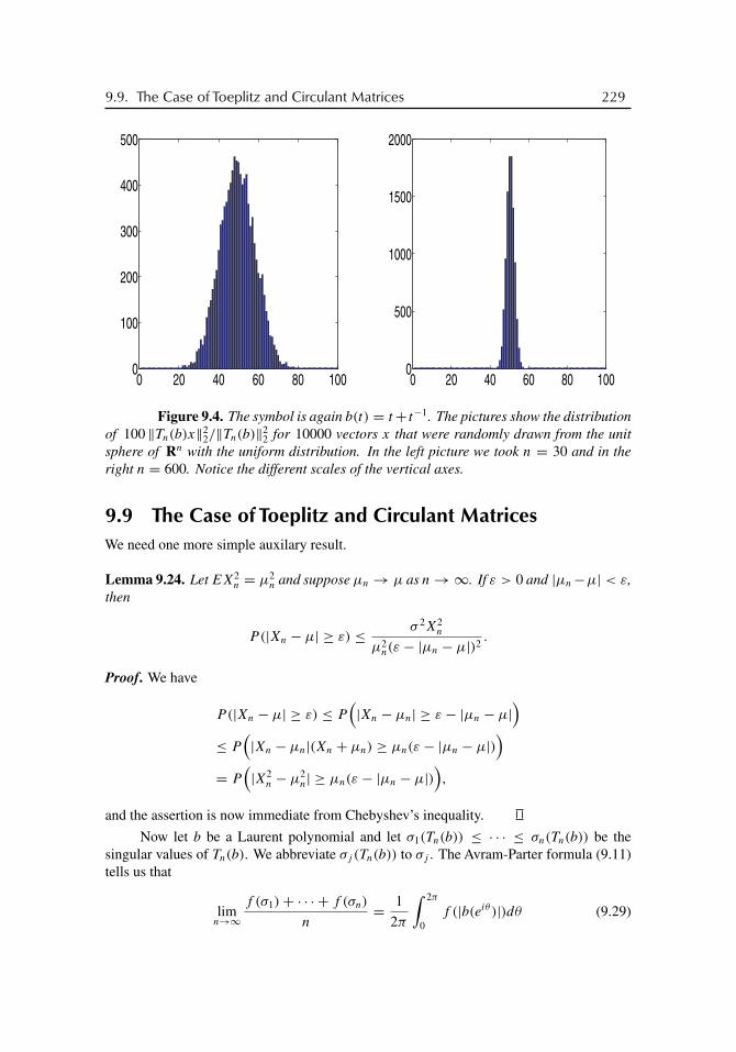
buch72005/10/5page 229

�

�

�

�

�

�

�

�

9.9. The Case of Toeplitz and Circulant Matrices 229

0 20 40 60 80 1000

100

200

300

400

500

0 20 40 60 80 1000

500

1000

1500

2000

Figure 9.4. The symbol is again b(t) = t+ t−1. The pictures show the distributionof 100 ‖Tn(b)x‖2

2/‖Tn(b)‖22 for 10000 vectors x that were randomly drawn from the unit

sphere of Rn with the uniform distribution. In the left picture we took n = 30 and in theright n = 600. Notice the different scales of the vertical axes.

9.9 The Case of Toeplitz and Circulant MatricesWe need one more simple auxilary result.

Lemma 9.24. Let EX2n = μ2

n and suppose μn → μ as n→∞. If ε > 0 and |μn−μ| < ε,then

P(|Xn − μ| ≥ ε) ≤ σ 2X2n

μ2n(ε − |μn − μ|)2

.

Proof. We have

P(|Xn − μ| ≥ ε) ≤ P(|Xn − μn| ≥ ε − |μn − μ|

)≤ P

(|Xn − μn|(Xn + μn) ≥ μn(ε − |μn − μ|)

)= P

(|X2

n − μ2n| ≥ μn(ε − |μn − μ|)

),

and the assertion is now immediate from Chebyshev’s inequality.

Now let b be a Laurent polynomial and let σ1(Tn(b)) ≤ · · · ≤ σn(Tn(b)) be thesingular values of Tn(b). We abbreviate σj (Tn(b)) to σj . The Avram-Parter formula (9.11)tells us that

limn→∞

f (σ1)+ · · · + f (σn)

n= 1

2π

∫ 2π

0f (|b(eiθ )|)dθ (9.29)

buch72005/10/5page 230

�

�

�

�

�

�

�

�


for every compactly supported function f : R → C with bounded variation. In particular,

limn→∞

σ k1 + · · · + σ k

n

n= ‖b‖k

k :=1

2π

∫ 2π

0|b(eiθ )|kdθ (9.30)

for every natural number k. Moreover, if T (b) is invertible, then σ1 = σ1(Tn(b)) stays awayfrom zero as n→∞ (Theorem 3.7), and hence (9.29) with f (s) equal to a negative integralpower of s times the characteristic function of [m, M] for appropriate 0 < m < M showsthat (9.30) is true for every integer k.

Theorem 9.25. If |b| is not constant on the unit circle T, then for each ε > 0 there is an n0

such that

P

( ∣∣∣∣ ‖Tn(b)x‖2

‖Tn(b)‖2 ‖x‖2− ‖b‖2

‖b‖∞∣∣∣∣ ≥ ε

)≤ 3

n+ 2

1

ε2

‖b‖44 − ‖b‖2

2

‖b‖22 ‖b‖2

∞(9.31)

for all n ≥ n0. If |b| is constant throughout T, then

P

( ‖Tn(b)x‖2

‖Tn(b)‖2 ‖x‖2≤ 1− ε

)= o

(1

n

)(9.32)

for each ε > 0.

Proof. Put

μn = 1

σn

√σ 2

1 + · · · + σ 2n

n, μ = ‖b‖2

‖b‖∞ .

Suppose first that |b| is not constant. Then ‖b‖4 > ‖b‖2. From (9.30) we know thatμn → μ. Moreover, (9.30) and Theorem 9.23 imply that

n+ 2

2σ 2X2

n →1

‖b‖4∞

(‖b‖4

4 − ‖b‖42

).

Thus, Lemma 9.24 shows that

P(|Xn − μ| ≥ ε) ≤ 3

n+ 2

1

‖b‖4∞

(‖b‖4

4 − ‖b‖42

) 1

μ2ε2

for all sufficiently large n, which is (9.31). On the other hand, if |b| is constant, we inferfrom (9.30) and Theorem 9.23 that

μn → 1 andn+ 2

2σ 2X2

n = o(1),

whence, by Lemma 9.24,

P(Xn ≤ 1− ε) ≤ 3

n+ 2o(1)

1

ε2= o

(1

n

),

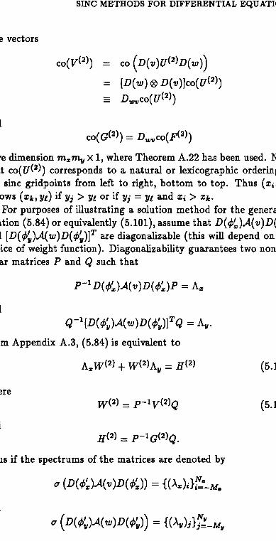
204 SING METHODS FOR DIFFERENTIAL EQUATIONS

The vectors

and

have dimension mxmy x 1, where Theorem A.22 has been used. Notethat co(Z/(2)) corresponds to a natural or lexicographic ordering ofthe sine gridpoints from left to right, bottom to top. Thus (zt>3/j)follows (xk, yi) if yj > yi or if yj = yi and z; > z*.

For purposes of illustrating a solution method for the general e-quation (5.84) or equivalently (5.101), assume that D(^)^4(v)JD(0!c)and [D((f>'y)A(w)D((j)'y)]

Tare diagonalizable (this will depend on thechoice of weight function). Diagonalizability guarantees two nonsin-gular matrices P and Q such that

and

From Appendix A.3, (5.84) is equivalent to

where

and

Thus if the spectrums of the matrices are denoted by

and

buch72005/10/5page 232

�

�

�

�

�

�

�

�


with 0 < σj ≤ σj+1 ≤ · · · ≤ σn and j ≤ k, and from Theorem 9.23 we infer that

EX2n =

1

nσ 2

j

(1

σ 2j

+ · · · + 1

σ 2n

)

= 1

n

(σ 2

j

σ 2j

+ · · · + σ 2j

σ 2k

)+ σ 2

j

n

(1

σ 2k+1

+ · · · + 1

σ 2n

)

≤ 1

n(k − j + 1)+ C2e−2γ n

n

n− k

λ2

≤ k

n+ C2e−2γ n

λ2≤ k + 1

n

for all sufficiently large n. Also by Theorem 9.23,

σ 2X2n =

2

n(n+ 2)σ 4

j

⎛⎝ 1

σ 4j

+ · · · + 1

σ 4n

− 1

n

(1

σ 2j

+ · · · + 1

σ 2n

)2⎞⎠ ,

and, analogously,

σ 4j

(1

σ 4j

+ · · · + 1

σ 4n

)≤ k + C4e−4γ n(n− k)

λ4≤ k + 1,

σ 4j

(1

σ 2j

+ · · · + 1

σ 2n

)2

≤(

k + C2e−2γ n(n− k)

λ2

)2

≤ (k + 1)2,

which gives σ 2X2n = O(1/n2). If ε > 0, then

P(Xn ≥ ε) = P(X2n ≥ ε2) ≤ P

(X2

n ≥k + 1

n+ ε2

2

)for all sufficiently large n, and thus,

P(Xn ≥ ε) ≤ P

(X2

n ≥ EX2n +

ε2

2

)≤ P

(|X2

n − EX2n| ≥

ε2

2

)≤ 4

ε4σ 2X2

n = O

(1

n2

).

Define the circulant matrices Cn(b) as in Section 2.1. The singular values of Cn(b)

are |b(ωjn)| (j = 0, . . . , n − 1), where ωn = e2πi/n. The only Laurent polynomials b of

constant modulus are b(t) = αtk (t ∈ T) with α ∈ C; in this case ‖Cn(b)x‖2 = |α| ‖x‖2

for all x.

Theorem 9.28. If |b| is not constant, then for each ε > 0 there exists an n0 such that

P

( ∣∣∣∣ ‖Cn(b)x‖2

‖Cn(b)‖2 ‖x‖2− ‖b‖2

‖b‖∞∣∣∣∣ ≥ ε

)≤ 3

n+ 2

1

ε2

‖b‖44 − ‖b‖2

2

‖b‖22 ‖b‖2∞

for all n ≥ n0.

buch72005/10/5page 233

�

�

�

�

�

�

�

�

9.10. The Nearest Structured Matrix 233

Proof. The proof is analogous to the proof of (9.31). Note that now (9.30) amounts to thefact that the integral sum

σ k1 + · · · + σ k

n

n=

n−1∑j=0

|b(e2πij/n)|k 1

n

converges to the Riemann integral∫ 1

0|b(e2πiθ )|kdθ =

∫ 2π

0|b(eiθ )|k dθ

2π=: ‖b‖k

k.

Furthermore, it is obvious that σn = max |b(ωjn)| → ‖b‖∞.

If b has no zeros on T, then C−1n (b) = Cn(b

−1), and hence Theorem 9.28 delivers

P

( ∣∣∣∣ ‖C−1n (b)x‖2

‖C−1n (b)‖2 ‖x‖2

− ‖b−1‖2

‖b−1‖∞∣∣∣∣ ≥ ε

)≤ 3

n+ 2

1

ε2

‖b−1‖44 − ‖b−1‖2

2

‖b−1‖22 ‖b−1‖2∞

(9.33)


9.10 The Nearest Structured MatrixWe denote by Mn(R) the linear space of all n×n matrices with real entries. Let An ∈ Mn(R)

and let 0 ≤ σ1 ≤ · · · ≤ σn be the singular values of An. Suppose σn > 0. The randomvariable X2

n = ‖Anx‖22/‖An‖2

2 assumes its values in [0, 1]. In this section we establish a fewresults on the distribution function of this random variable and we give a nice applicationto the problem of describing in probabilistic terms the distance of a matrix to the nearestmatrix of a given structure. With notation as in the proof of Theorem 9.23,

Eξ :={x ∈ Sn−1 : ‖Anx‖2

2

‖An‖22

< ξ

}=

{x ∈ Sn−1 : ‖DnVnx‖2

2

σ 2n

< ξ

}.

Put Gξ = {x ∈ Sn−1 : ‖Dnx‖22/σ

2n < ξ}. Clearly, Gξ = Vn(Eξ ). Since Vn is an orthogonal

matrix, it leaves the surface measure on Sn−1 invariant. It follows that |Gξ | = |Vn(Eξ )| andhence

Fn(ξ) := P(X2n < ξ) = P

(‖Dnx‖22

σ 2n

< ξ

)= P

(σ 2

1 x21 + · · · + σ 2

n x2n

σ 2n

< ξ

). (9.34)

This reveals first of all that the distribution function Fn(ξ) depends only on the singularvalues of An. We let fn(ξ) stand for the density function corresponding to the distributionfunction Fn(ξ).

A real-valued random variable X is said to be B(α, β) distributed on (a, b) if

P(c ≤ X < d) =∫ d

c

f (ξ) dξ,

where the density function f (ξ) is zero on (−∞, a] and [b,∞) and equals

(b − a)1−α−β

B(α, β)(ξ − a)α−1(b − ξ)β−1

buch72005/10/5page 234

�

�

�

�

�

�

�

�


on the interval (a, b). Here

B(α, β) = �(α)�(β)

�(α + β)

is the common beta function and it is assumed that α > 0 and β > 0.We first consider 2× 2 matrices, that is, we let n = 2. From (9.34) we infer that

F2(ξ) = P

(σ 2

1

σ 22

x21 + x2

2 < ξ

). (9.35)

The constellation σ1 = σ2 is uninteresting, because F2(ξ) = 0 for ξ < 1 and F2(ξ) = 1 forξ ≥ 1 in this case.

Theorem 9.29. If σ1 < σ2, then the random variable X22 is subject to the B( 1

2 , 12 ) distribution

on (σ 21 /σ 2

2 , 1).

Proof. Put τ = σ1/σ2. By (9.35), F2(ξ) is 12π

times the length of the piece of the unitcircle x2

1 + x22 = 1 that is contained in the interior of the ellipse τ 2x2

1 + x22 = ξ . This gives

F2(ξ) = 0 for ξ ≤ τ 2 and F2(ξ) = 1 for ξ ≥ 1. Thus, let ξ ∈ (τ 2, 1). Then the circle andthe ellipse intersect at the four points⎛⎝±√

1− ξ

1− τ 2, ±

√ξ − τ 2

1− τ 2

⎞⎠ ,

and consequently,

F2(ξ) = 2

πarctan

√ξ − τ 2

1− ξ,

which implies that F ′2(ξ) equals

1

π(ξ − τ 2)−1/2(1− ξ)−1/2 = 1

B(1/2, 1/2)(ξ − τ 2)−1/2(1− ξ)−1/2

and proves that X22 has the B( 1

2 , 12 ) distribution on (τ 2, 1).

In the case n ≥ 3, things are more involved. An idea of the variety of possibledistribution functions is provided by the class of matrices whose singular values satisfy

0 = σ1 = · · · = σn−2 < σn−1 < σn.

For y ∈ (0, 1), the complete elliptic integrals K(y) and E(y) are defined by

K(y) =∫ π/2

0

dϕ√1− y2 sin2 ϕ

, E(y) =∫ π/2

0

√1− y2 sin2 ϕ dϕ.

buch72005/10/5page 235

�

�

�

�

�

�

�

�

9.10. The Nearest Structured Matrix 235

Put μ = σn/σn−1. In [52], we showed that on (0, 1/μ2) one has the following densities:

f3(ξ) = μ

π√

1− ξK

⎛⎝√ξ(μ2 − 1)

1− ξ

⎞⎠ ,

f4(ξ) = μ (uniform distribution),

f5(ξ) = 3μ√

1− ξ

πE

⎛⎝√ξ(μ2 − 1)

1− ξ

⎞⎠ ,

f6(ξ) = 2μ− μ(μ2 + 1)ξ ,

and f7(ξ) equals

5μ

3π

√1− ξ

⎛⎝(4− 2ξ − 2ξμ2) E

⎛⎝√ξ(μ2 − 1)

1− ξ

⎞⎠− (1− ξμ2) K

⎛⎝√ξ(μ2 − 1)

1− ξ

⎞⎠⎞⎠ .

In some particular cases, one gets a complete answer. Here is an example.

Theorem 9.30. Let n ≥ 3. If σ1 = · · · = σn−m = 0 and σn−m+1 = · · · = σn > 0, then therandom variable X2

n is B(m2 , n−m

2 ) distributed on (0, 1).

This can be proved by the argument of the proof of Theorem 9.29, the only difference beingthat now one has to compute some multidimensional integrals. A full proof is in [52].

Orthogonal projections have just the singular value pattern of Theorem 9.30. Thisleads to some pretty nice conclusions. Let E be an N -dimensional Euclidean space and letU be an m-dimensional linear subspace of E. We denote by PU the orthogonal projectionof E onto U . Then for y ∈ E, the element PUy is the best approximation of y in U and wehave ‖y‖2 = ‖PUy‖2 + ‖y − PUy‖2. The singular values of PU are N − m zeros and m

units. Thus, Theorem 9.30 implies that if y is uniformly distributed on the unit sphere ofE, then ‖PUy‖2 has the B(m

2 , N−m2 ) distribution on (0, 1). In particular, if N is large, then

PUy lies with high probability close to the sphere of radius√

mN

and the squared distance‖y − PUy‖2 clusters sharply around 1− m

N.

Now take E = Mn(R). With the Frobenius norm ‖ · ‖F, E is an n2-dimensionalEuclidean space. Let U = Strn(R) denote any class of structured matrices that form anm-dimensional linear subspace of Mn(R). Examples include

the Toeplitz matrices, Toepn(R)

the Hankel matrices, Hankn(R)

the tridiagonal matrices, Tridiagn(R)

the tridiagonal Toeplitz matrices, TridiagToepn(R)

the symmetric matrices, Symmn(R)

the lower-triangular matrices, Lowtriangn(R)

the matrices with zero main diagonal, Zerodiagn(R)

the matrices with zero trace, Zerotracen(R).

buch72005/10/5page 236

�

�

�

�

�

�

�

�


The dimensions of these linear spaces are

dim Toepn(R) = 2n− 1, dim Hankn(R) = 2n− 1,

dim Tridiagn(R) = 3n− 2, dim TridiagToepn(R) = 3,

dim Symmn(R) = n2 + n

2, dim Lowtriangn(R) = n2 + n

2,

dim Zerodiagn(R) = n2 − n, dim Zerotracen(R) = n2 − 1.

Suppose n is large and Yn ∈ Mn(R) is uniformly distributed on the unit sphere on Mn(R),‖Yn‖2

F = 1. Let PStrYn be the best approximation of Yn by a matrix in Strn(R). Notice thatthe determination ofPStrYn is a least squares problem that can be easily solved. For instance,PToepYn is the Toeplitz matrix whose kth diagonal, k = −(n− 1), . . . , n− 1, is formed bythe arithmetic mean of the numbers in the kth diagonal of Yn. Recall that dim Strn(R) = m.From what was said in the preceding paragraph, we conclude that ‖PStrYn‖2

F is B(m2 , n2−m

2 )

distributed on (0, 1). For example, ‖PToepYn‖2 has the B( 2n−12 , n2−2n+1

2 ) distribution on(0, 1). The expected value of the variable ‖Yn − PToepYn‖2 is 1− 2

n+ 1

n2 and the variancedoes not exceed 4

n3 . Hence, Chebyshev’s inequality gives

P

(1− 2

n+ 1

n2− ε

n< ‖Yn − PToepYn‖2 < 1− 2

n+ 1

n2+ ε

n

)≥ 1− 4

nε2. (9.36)

Consequently, PToepYn is with high probability found near the sphere with the radius√2n− 1

n2 and ‖Yn − PToepYn‖2F is tightly concentrated around 1− 2

n+ 1

n2 .

We arrive at the conclusion that nearly all n× n matrices of Frobenius norm 1 are atnearly the same distance to the set of all n× n Toeplitz matrices!

This does not imply that the Toeplitz matrices are at the center of the universe. Infact, the conclusion is true for each of the classes Strn(R) listed above. For instance, fromChebyshev’s inequality we obtain

P

(1

2− 1

2n− ε < ‖Yn − PSymmYn‖2 <

1

2− 1

2n+ ε

)≥ 1− 1

2n2ε2(9.37)

and

P

(1

n2− ε

n2< ‖Yn − PZerotraceYn‖2 <

1

n2+ ε

n2

)≥ 1− 2

n2ε2.

If the expected value of ‖Yn − PStructYn‖2 stays away from 0 and 1 as n → ∞, we havemuch sharper estimates. Namely, Lemma 2.2 of [93] in conjunction with Theorem 9.30implies that if X2

n has the B(m2 , N−m

2 ) distribution on (0, 1), then

P(X2

n ≤ σm

N

)≤ (

σe1−σ)m/2

, P(X2

n ≥ τm

N

)≤ (

τe1−τ)m/2

(9.38)

for 0 < σ < 1 < τ . This yields, for example,

P

(σ

(1

2− 1

2n

)< ‖Yn − PSymmYn‖2

F < τ

(1

2− 1

2n

))≥ 1− (

σe1−σ)(n2+n)/4 − (

τe1−τ)(n2+n)/4

(9.39)

buch72005/10/5page 237

�

�

�

�

�

�

�

�

Exercises 237

whenever 0 < σ < 1 < τ . Clearly, (9.39) is better than (9.37). On the other hand,let ε > 0 be small and choose τ such that τ (1 − 2

n+ 1

n2 ) = 1 − 2n+ 1

n2 + εn

. Then

(τe1−τ )n−1/2 = 1− ε2

2n+O ( 1

n2 ), the O depending on ε, and hence (9.38) amounts to

P

(‖Yn − PToepYn‖2 ≥ 1− 2

n+ 1

n2+ ε

n

)≤ 1− ε2

2n+O

(1

n2

),

which is worse than the Chebyshev estimate (9.36).

Exercises

1. Let �pn be the space Cn with the �p norm. Does every n × n matrix An have a

representation An = UnSnVn where Un and Vn induce invertible isometries on �pn and

Sn is a diagonal matrix?

2. Let {An}, {Bn}, {En}, {Rn} be sequences of n× n matrices and suppose

An = Bn + En + Rn, ‖En‖2F = o(n), rank Rn = o(n).

Let λj (Cn) and σj (Cn) (j = 1, . . . , n) denote the eigenvalues and singular values ofan n× n matrix Cn.

(a) Prove that if, in addition, An, Bn, En, Rn are all Hermitian, then the eigenvaluesof An and Bn are tied by the relation

limn→∞

1

n

n∑j=1

[ϕ(λj (An))− ϕ(λj (Bn))

] = 0

for every continuous function ϕ : R → C with compact support.

(b) Show that if Cn is an arbitrary n× n matrix and Hn denotes the Hermitian matrix(

0 Cn

C∗n 0 ), then

{λ1(Hn), . . . , λ2n(Hn)} = {σ1(Cn), . . . , σn(Cn),−σ1(Cn), . . . ,−σn(Cn)}.(c) Deduce from (a) and (b) that the singular values of An and Bn satisfy

limn→∞

1

n

n∑j=1

[ϕ(σj (An))− ϕ(σj (Bn))

] = 0

for every compactly supported continuous function ϕ : R → C.

3. Let X1, . . . , Xn be independent random variables subject to the Gaussian normaldistribution with mean 0 and variance 1. Show that

(X1, . . . , Xn)√X2

1 + · · · +X2n

is uniformly distributed on the unit sphere Sn−1.

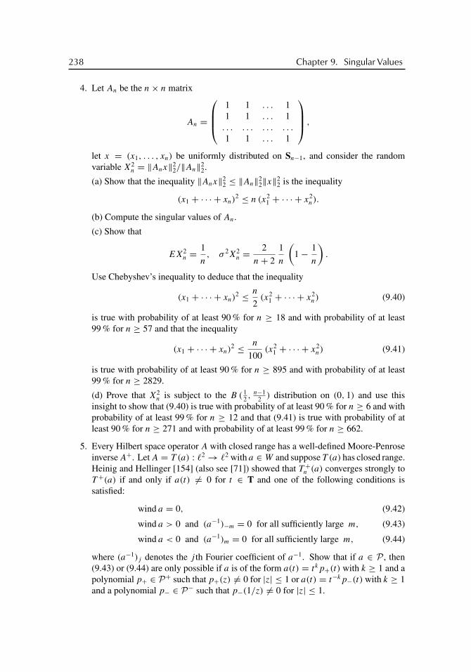
buch72005/10/5page 238

�

�

�

�

�

�

�

�


4. Let An be the n× n matrix

An =

⎛⎜⎜⎝1 1 . . . 11 1 . . . 1. . . . . . . . . . . .

1 1 . . . 1

⎞⎟⎟⎠ ,

let x = (x1, . . . , xn) be uniformly distributed on Sn−1, and consider the randomvariable X2

n = ‖Anx‖22/‖An‖2

2.

(a) Show that the inequality ‖Anx‖22 ≤ ‖An‖2

2‖x‖22 is the inequality

(x1 + · · · + xn)2 ≤ n (x2

1 + · · · + x2n).

(b) Compute the singular values of An.

(c) Show that

EX2n =

1

n, σ 2X2

n =2

n+ 2

1

n

(1− 1

n

).

Use Chebyshev’s inequality to deduce that the inequality

(x1 + · · · + xn)2 ≤ n

2(x2

1 + · · · + x2n) (9.40)

is true with probability of at least 90 % for n ≥ 18 and with probability of at least99 % for n ≥ 57 and that the inequality

(x1 + · · · + xn)2 ≤ n

100(x2

1 + · · · + x2n) (9.41)

is true with probability of at least 90 % for n ≥ 895 and with probability of at least99 % for n ≥ 2829.

(d) Prove that X2n is subject to the B ( 1

2 , n−12 ) distribution on (0, 1) and use this

insight to show that (9.40) is true with probability of at least 90 % for n ≥ 6 and withprobability of at least 99 % for n ≥ 12 and that (9.41) is true with probability of atleast 90 % for n ≥ 271 and with probability of at least 99 % for n ≥ 662.

5. Every Hilbert space operator A with closed range has a well-defined Moore-Penroseinverse A+. Let A = T (a) : �2 → �2 with a ∈ W and suppose T (a) has closed range.Heinig and Hellinger [154] (also see [71]) showed that T +n (a) converges strongly toT +(a) if and only if a(t) �= 0 for t ∈ T and one of the following conditions issatisfied:

wind a = 0, (9.42)

wind a > 0 and (a−1)−m = 0 for all sufficiently large m, (9.43)

wind a < 0 and (a−1)m = 0 for all sufficiently large m, (9.44)

where (a−1)j denotes the j th Fourier coefficient of a−1. Show that if a ∈ P , then(9.43) or (9.44) are only possible if a is of the form a(t) = t kp+(t) with k ≥ 1 and apolynomial p+ ∈ P+ such that p+(z) �= 0 for |z| ≤ 1 or a(t) = t−kp−(t) with k ≥ 1and a polynomial p− ∈ P− such that p−(1/z) �= 0 for |z| ≤ 1.

buch72005/10/5page 239

�

�

�

�

�

�

�

�

Notes 239

6. To compute the numerical range H2(An) = {(Anx, x) : ‖x‖2 = 1} of an n × n

matrix An one could try drawing a large number N of random vectors xj from theuniform distribution on the unit sphere of Cn and plotting the superposition of thevalues (Anxj , xj ) (j = 1, . . . , N). In the right picture of Figure 9.5 we see the resultfor An = Tn(b) with b as in Figure 7.1, n = 50 and N = 500. As the numericalrange contains at least the convex hull of the eigenvalues, which are shown in the leftpicture, we conclude that our experiment failed dramatically. Why did it fail?

−20 −10 0 10 20−30

−25

−20

−15

−10

−5

0

5

10

15

20

−20 −10 0 10 20−30

−25

−20

−15

−10

−5

0

5

10

15

20

Figure 9.5. We see the range b(T) and the 50 eigenvalues of T50(b) (left) and thevalues (T50(b)x, x) for 500 vectors x drawn randomly from the uniform distribution on theunit sphere of C50 (right).

Notes

Proofs of the theorems of Section 9.1 are in [27], [133], [166], for example.The splitting phenomenon, Theorem 9.4, was discovered by Roch and Silbermann

[224], [225]. They proved Theorem 9.4 for p = 2 and their proof is based on C∗-algebratechniques. In [35], another proof was given and the result was extended to 1 ≤ p ≤ ∞.Estimate (9.2) was established in our paper [47]. The proof of Theorem 9.4 presented hereis a combination of arguments of [35] and [48].

The idea of deriving results on Toeplitz matrices by comparing Toeplitz matrices withtheir circulant cousins has been developed by Shigeru Arimoto and coauthors in a series ofpapers since about 1985 which deal with problems of theoretical chemistry and in whichsequences of banded circulant matrices are called alpha matrices. Independently, the sameidea has emerged in papers by Beam and Warming [20], Tyrtyshnikov [284], and SerraCapizzano and Tilli [251]. Theorems 9.6 to 9.9 are from our book [48], but we are surethat versions of these theorems had been known earlier. We noticed in [48] that we foundthese theorems in our manuscripts but that we cannot remember whether we obtained themourselves some time ago or whether we took them from somewhere.

Theorems 9.7 and 9.19 can be found in [27] and [167]. We thank Estelle Basor forpointing out that Theorem 9.7 was incorrectly stated in our previous book [48].

buch72005/10/5page 240

�

�

�

�

�

�

�

�


Formula (9.9) is Widom’s [295] and its generalization (9.8) is due to Roch and Sil-bermann [222].

Formula (9.11), the so-called Avram-Parter theorem, was established by Parter [200]for symbols b ∈ L∞ which are locally normal, that is, which can be written as the productof a continuous and a real-valued function. Avram [10] proved (9.11) for general b ∈ L∞.We refer the reader to Sections 5.6 and 5.8 of [71] and to [301] for further generalizationsof the Avram-Parter theorem. The elegant approach and the results of Section 9.6 are dueto Zizler, Zuidwijk, Taylor, and Arimoto [303]. The notions of the cluster and the propercluster were introduced by Tyrtyshnikov in [284].

Sections 9.8 to 9.10 are based on our paper [52].A solution to Exercise 1 is in [71] (see also [250]). Exercise 2 is a result of Tyrtyshnikov

[282], [284].

Further results: C∗-algebras I. The purpose of the following is to illustrate how a fewsimple C∗-algebra arguments yield part of the results established in the previous chaptersvery quickly. Of course, the C∗ machinery forces us to limit ourselves to the case p = 2.

A Banach algebra is a complex Banach space A with an associative and distributivemultiplication such that ‖ab‖ ≤ ‖a‖ ‖b‖ for all a, b ∈ A. If a Banach algebra has a unitelement, which is usually denoted by e, 1, or I , it is referred to as a unital Banach algebra.A conjugate-linear map a �→ a∗ of a Banach algebra into itself is called an involution ifa∗∗ = a and (ab)∗ = b∗a∗ for all a, b ∈ A. Finally, a C∗-algebra is a Banach algebra withan involution such that ‖a∗a‖ = ‖a‖2 for all a ∈ A. Notice that C∗-algebras are especiallynice Banach algebras, although the terminology suggests the contrary.

If H is a Hilbert space, then the sets B(H) and K(H) of all bounded and compactlinear operators on H are C∗-algebras under the operator norm and passage to the Hermitianadjoint as involution. This is in particular the case for B := B(�2) and K := K(�2). Clearly,B is unital, but K has no unit element. The set C := C(T) is a C∗-algebra under the norm‖ · ‖∞ and the involution a �→ a (passage to the complex conjugate). The Wiener algebraW is a Banach algebra with an involution, a �→ a, but it is not a C∗-algebra, because theequality ‖aa‖W = ‖a‖2

W is not satisfied for all a ∈ W . In the case p = 2, the Banachalgebras F and S introduced in Section 3.4 are C∗-algebras. The involution is defined by{An}∗ := {A∗n}.

A subset of a C∗-algebraA that is itself a C∗-algebra is called a C∗-subalgebra. LetAbe a C∗-algebra and let E be a subset of A. The C∗-algebra generated by E is the smallestC∗-subalgebra of A that contains E. (In other words, the C∗-algebra generated by E is theintersection of all C∗-subalgebras of A that contain E.) If this C∗-algebra is A itself, onesays that A is generated by E.

One of the many excellent properties of C∗-algebras is their inverse closedness. Thismeans the following. If A1 is a unital C∗-algebra with the unit element e and A2 is aC∗-subalgebra of A1 which contains e, then every element a ∈ A2 that is invertible in A1

is automatically invertible in A2.So far we have considered the Toeplitz operator T (a) for a ∈ W only. For a ∈ C

(or even a ∈ L∞(T)), this operator is also defined via the matrix (aj−k)∞j,k=1 formed of the

Fourier coefficients. It is not difficult to prove that T (a) is bounded on �2 for a ∈ C (oreven a ∈ L∞(T)). If b ∈ P , then the sequence {Tn(b)} is an element of the C∗-algebra F.Let A denote the C∗-algebra generated by E = {{Tn(b)} : b ∈ P} in F. Let finally G be the

buch72005/10/5page 241

�

�

�

�

�

�

�

�

Notes 241

set of all {An} ∈ F for which ‖An‖2 → 0 as n→∞.

Theorem on A. The C∗-algebra A is the set of all sequences {An} of the form

An = Tn(a)+ PnKPn +WnLWn + Cn (9.45)

with a ∈ C, K ∈ K, L ∈ K, {Cn} ∈ G.

This theorem was established in [66] (proofs are also in [70, Proposition 7.27] and[62, Proposition 2.2]).

A C∗-algebra homomorphism is a map f : A1 → A2 of a C∗-algebra A1 into aC∗-algebra A2 satisfying

f (αa) = αf (a), f (a + b) = f (a)+ f (b), f (ab) = f (a)f (b), f (a∗) = f (a)∗

for all α ∈ C, a ∈ A1, b ∈ A1. The set G is obviously a closed two-sided ideal of theC∗-algebra A. Therefore the quotient algebra A/G is a C∗-algebra with the usual quotientoperations and the usual quotient norm. The sumB⊕B is the C∗-algebra of all ordered pairs(A, B) ∈ B2 with the natural operations and the norm ‖(A, B)‖ := max(‖A‖2, ‖B‖2). Let{An} be given by (9.45). Then

An → A := T (a)+K and WnAnWn → A := T (a)+ L

strongly as n→∞.

Theorem on A/G. The map Sym defined by

Sym : A/G → B ⊕ B, {An} +G �→ (A, A)

is a C∗-algebra homomorphism that preserves spectra and norms.

It is easily verified that Sym is a C∗-algebra homomorphism. Since the only compactToeplitz operator is the zero operator (this is Corollary 1.13 for a ∈ C), it follows that Sym isinjective. As injective homomorphisms of unital C∗-algebras automatically preserve spectraand norms (which is another exquisite property of C∗-algebras that is not shared by generalBanach algebras), we arrive at the conclusion of the theorem. This simple reasoning goesback to [66], [70, Theorem 7.11] and is explicit in [34].

Here are some immediate consequences of the theorem on A/G.

Consequence 1. A sequence {An} ∈ A is stable on �2 if and only if A = T (a) + K

and A = T (a)+L are invertible on �2 (Theorem 3.13 for p = 2). Indeed, due to the inverseclosedness of A/G in F/G, the stability of {An} is equivalent to the condition that 0 doesnot belong to the spectrum of {An} +G in A/G.

Consequence 2. If {An} ∈ A and both A and A are invertible on �2, then

A−1n = Tn(a

−1)+ PnXPn +WnYWn +Dn (9.46)

with X ∈ K, Y ∈ K, {Dn} ∈ G for all sufficiently large n (recall Section 3.5). Indeed, theassumption implies that ({An}+G)−1 ∈ A/G and the theorem on A therefore yields (9.46).Passing to the strong limit n→∞ in (9.46) we get

T −1(a) = T (a−1)+X and T −1(a) = T (a−1)+ Y,

buch72005/10/5page 242

�

�

�

�

�

�

�

�


that is, we recover (3.15) and (3.16).

Consequence 3. If {An} ∈ A, then

limn→∞‖An‖2 = max(‖A‖2, ‖A‖2)

(Corollary 5.14 for p = 2). This follows from Theorem 3.1 and the equalities

lim supn→∞

‖An‖2 = ‖{An} +G‖A/G = ‖Sym ({An} +G)‖B⊕B = max(‖A‖2, ‖A‖2).

Consequence 4. If {An} ∈ A and A and A are invertible on �2, then

limn→∞‖A

−1n ‖2 = max(‖A−1‖2, ‖A−1‖2)

(Theorem 6.3 for p = 2). To see this, combine Consequences 2 and 3.

Consequence 5. If {An} ∈ A and at least one of the operators A and A is nonzero,then

limn→∞ κ2(An) = max(‖A‖2, ‖A‖2) max(‖A−1‖2, ‖A−1‖2)

(Corollary 6.4 for p = 2). This is straightforward from Consequences 3 and 4.

Consequence 6. If {An} ∈ A and ε > 0, then

lim infn→∞ sp(2)

ε An = lim supn→∞

sp(2)ε An = sp(2)

ε A ∪ sp(2)ε A

(generalization of Theorem 7.7 in the case p = 2). Once Consequence 4 is available, thiscan be proved by the argument of the proof of Theorem 7.7.

Consequence 7. If {An} ∈ A and A∗n = An for all n, then


n→∞sp An = sp A ∪ sp A

(Lemma 9.10). To see this, let λ /∈ sp A∪ sp A. Then {An − λI } is stable (Consequence 1)and hence the spectral radius of (An−λI)−1 remains bounded as n→∞. This implies thatλ /∈ lim sup sp An. Conversely, let λ ∈ R and λ /∈ lim inf sp An. Then there exists a δ > 0such that Uδ(λ) ∩ sp An = ∅ for infinitely many n, that is, Uδ(0) ∩ sp (An − λI) = ∅ forinfinitely many n. As An−λI is Hermitian, the spectral radius and the norm of (An−λI)−1

coincide, which gives that ‖(An − λI)−1‖2 ≤ 1/δ for infinitely many n. Consequently,we arrive at a subsequence {nk} such that {Ank

− λI } and thus also {Wnk(Ank

− λI)Wnk} is

stable. Lemma 3.4 now yields the invertibility of A− λI and A− λI .

Consequence 8. If {An} ∈ A, then

lim infn→∞ �(An) = lim sup

n→∞�(An) = �(A) ∪�(A)

(Corollary 9.11). Since {A∗nAn} ∈ A, this follows from Consequence 7.

Summary. Thus, we have demonstrated that many sharp convergence results can beobtained very comfortably by working with appropriate C∗-algebras. For more details and

buch72005/10/5page 243

�

�

�

�

�

�

�

�

Notes 243

for further developments of this idea we refer the reader to [36], [48], [223] and especiallyto Hagen, Roch, and Silbermann’s monograph [149]. Another approach to questions ofnumerical analysis via C∗-algebras was worked out by Arveson [7], [8], [9]. Fragments ofthis approach will be outlined in the notes to Chapter 14.

We nevertheless want to emphasize that the C∗-algebra approach has its limitations.For example, it is restricted to Hilbert space operators. Moreover, refinements of the conse-quences cited above, such as estimates of the convergence speed, require hard analysis andhence the tools presented in the preceding chapters.

buch72005/10/5page 244

�

�

�

�

�

�

�

�

buch72005/10/5page 245

�

�

�

�

�

�

�

�

Chapter 10

ExtremeEigenvalues

In this chapter we embark on the extreme eigenvalues of Hermitian Toeplitz matrices andon estimates for the spectral radius of not necessarily Hermitian Toeplitz matrices.

10.1 Hermitian MatricesLet b be a nonconstant Laurent polynomial. The matrix Tn(b) is Hermitian if and only ifbj = b−j , that is, if and only if b is real valued. So suppose b is real valued and let

m = mint∈T

b(t), M = maxt∈T

b(t).

By Lemma 4.7,

(Tn(b)x, x) = 1

2π

∫ 2π

0b(eiθ )|f (eiθ )|2dθ, (10.1)

where f (eiθ ) = x0 + x1eiθ + · · · + xn−1e

i(n−1)θ . This implies that all eigenvalues of Tn(b)

are contained in the open interval (m, M),

m < λ1(Tn(b)) ≤ λ2(Tn(b)) ≤ · · · ≤ λn(Tn(b)) < M. (10.2)

Theorem 10.1. Let b be a nonconstant real-valued Laurent polynomial, let R(b) = [m, M],and denote by 2α and 2β the maximal order of the zeros of b−m and M − b, respectively.Then for each fixed k,

λk(Tn(b))−m � 1

n2α, M − λn−k(Tn(b)) � 1

n2β,

where the notation xn � yn means that there are constants C1, C2 ∈ (0,∞) such thatC1yn ≤ xn ≤ C2yn for all sufficiently large n.

Proof. Put a = b − m. Then, by (10.1), (Tn(a)x, x) ≥ 0 for all x ∈ �2n. This shows

that (T ∗n (a)Tn(a))1/2 = (Tn(a)Tn(a))1/2 = Tn(a). Consequently, the eigenvalues of Tn(a)

245

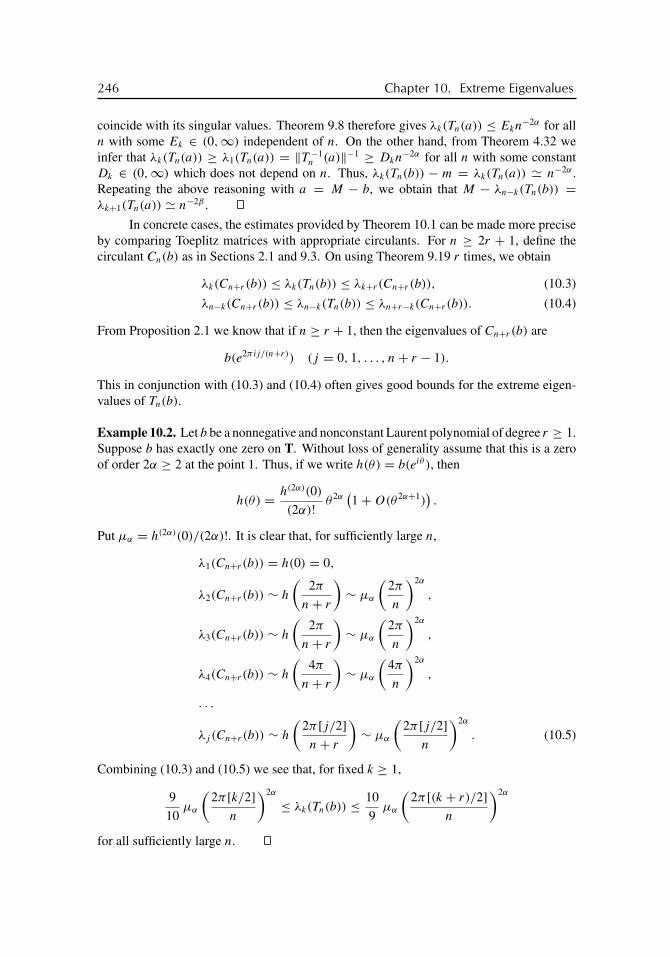
buch72005/10/5page 246

�

�

�

�

�

�

�

�

246 Chapter 10. Extreme Eigenvalues

coincide with its singular values. Theorem 9.8 therefore gives λk(Tn(a)) ≤ Ekn−2α for all

n with some Ek ∈ (0,∞) independent of n. On the other hand, from Theorem 4.32 weinfer that λk(Tn(a)) ≥ λ1(Tn(a)) = ‖T −1

n (a)‖−1 ≥ Dkn−2α for all n with some constant

Dk ∈ (0,∞) which does not depend on n. Thus, λk(Tn(b)) − m = λk(Tn(a)) � n−2α .Repeating the above reasoning with a = M − b, we obtain that M − λn−k(Tn(b)) =λk+1(Tn(a)) � n−2β .

In concrete cases, the estimates provided by Theorem 10.1 can be made more preciseby comparing Toeplitz matrices with appropriate circulants. For n ≥ 2r + 1, define thecirculant Cn(b) as in Sections 2.1 and 9.3. On using Theorem 9.19 r times, we obtain

λk(Cn+r (b)) ≤ λk(Tn(b)) ≤ λk+r (Cn+r (b)), (10.3)

λn−k(Cn+r (b)) ≤ λn−k(Tn(b)) ≤ λn+r−k(Cn+r (b)). (10.4)

From Proposition 2.1 we know that if n ≥ r + 1, then the eigenvalues of Cn+r (b) are

b(e2πij/(n+r)) (j = 0, 1, . . . , n+ r − 1).

This in conjunction with (10.3) and (10.4) often gives good bounds for the extreme eigen-values of Tn(b).

Example 10.2. Let b be a nonnegative and nonconstant Laurent polynomial of degree r ≥ 1.Suppose b has exactly one zero on T. Without loss of generality assume that this is a zeroof order 2α ≥ 2 at the point 1. Thus, if we write h(θ) = b(eiθ ), then

h(θ) = h(2α)(0)

(2α)! θ2α(1+O(θ2α+1)

).

Put μα = h(2α)(0)/(2α)!. It is clear that, for sufficiently large n,

λ1(Cn+r (b)) = h(0) = 0,

λ2(Cn+r (b)) ∼ h

(2π

n+ r

)∼ μα

(2π

n

)2α

,

λ3(Cn+r (b)) ∼ h

(2π

n+ r

)∼ μα

(2π

n

)2α

,

λ4(Cn+r (b)) ∼ h

(4π

n+ r

)∼ μα

(4π

n

)2α

,

. . .

λj (Cn+r (b)) ∼ h

(2π [j/2]n+ r

)∼ μα

(2π [j/2]

n

)2α

. (10.5)

Combining (10.3) and (10.5) we see that, for fixed k ≥ 1,

9

10μα

(2π [k/2]

n

)2α

≤ λk(Tn(b)) ≤ 10

9μα

(2π [(k + r)/2]

n

)2α


buch72005/10/5page 247

�

�

�

�

�

�

�

�

10.1. Hermitian Matrices 247

Although the eigenvalue distribution of Toeplitz band matrices will be the subjectof the next chapter, we already now have everything at our disposal in order to treat theHermitian case.

Since sp Tn(b) = m+ sp Tn(b−m) and since the eigenvalues of Tn(b−m) coincidewith the singular values of Tn(b − m), we can have immediate recourse to the results ofSection 9.4. However, since Theorem 9.19 is a little bit sharper than Theorem 9.7, repetitionof the reasoning of Section 9.6 with Theorem 9.7 replaced by Theorem 9.19 yields slightlybetter results. We begin with the analogue of Theorem 9.14.

Theorem 10.3. Let r and n be natural numbers such that 1 ≤ r < n, let K = {k1, . . . , kr}be a subset of {1, 2, . . . , n} consisting of r distinct elements, and put L = {1, 2, . . . , n}\K .Suppose A and A′ are two Hermitian n × n matrices whose jk entries coincide for all(j, k) ∈ L × L. If f ∈ BV and [a, b] is any segment which contains the eigenvalues ofboth A and A′, then

n∑k=1

∣∣f (λk(A))− f (λk(A′))

∣∣ ≤ rV[a,b](f ).

Proof. We proceed exactly as in the proof of Theorem 9.14. Define B as in that proof. NowTheorem 9.19 gives

λ1(A), λ1(A′) ∈ [a, λ1(B)],

λ2(A), λ2(A′) ∈ [λ1(B), λ2(B)],

. . .

λn−1(A), λn−1(A′) ∈ [λn−2(B), λn−1(B)],

λn(A), λn(A′) ∈ [λn−1(B), b],

whence, as in the proof of Theorem 9.14,

n∑k=1

∣∣f (λk(A))− f (λk(A′))

∣∣ ≤ V[a,λ1](f )+ V[λ1,λ2](f )+ · · · + V[λn−1,b](f ) = V[a,b](f )

with λj := λj (B). Thus, the factor 3 that we encountered in the proof of Theorem 9.14disappears.

Theorem 10.4. Let b(t) = ∑rj=−r bj t

j (t ∈ T) be a nonconstant real-valued Laurentpolynomial and let f ∈ BV . If [c, d] is any segment which containsR(b) = [min b, max b],then for all n ≥ 1,∣∣∣∣∣

n∑k=1

f (λk(Tn(b)))− n

2π

∫ 2π

0f (b(eiθ ))dθ

∣∣∣∣∣ ≤ 3rV[c,d](f ).

Proof. This follows from the reasoning of the proof of Theorem 9.15. In (9.14) we can dropthe factor 3, and considering u(θ) = b(eiθ ) instead of u(θ) = |b(eiθ )|2, we can replace thefactor 4 in (9.16) by the factor 2. This gives the assertion.

buch72005/10/5page 248

�

�

�

�

�

�

�

�


Corollary 10.5. Let b be a real-valued Laurent polynomial and let f : R → C be a functionwith compact support. If f is continuous or of bounded variation, then

limn→∞

1

n

n∑k=1

f (λk(Tn(b))) = 1

2π

∫ 2π

0f (b(eiθ ))dθ.

Proof. Use the same arguments as in the proof of Corollary 9.16.

Given a (Lebesgue) measurable subset E of R, we put

Nn(E) =n∑

k=1

χE(λk(Tn(b))), μn(E) = 1

nNn(E),

μ(E) = 1

2π

∫ 2π

0χE(b(eiθ ))dθ = 1

2π|{t ∈ T : b(t) ∈ E}|,

where | · | is Lebesgue measure on T. In the same way we proved Corollaries 9.17 and 9.18we now obtain the following two results.

Corollary 10.6. Let b be a real-valued Laurent polynomial. Then∫R

f dμn →∫

Rf dμ

for every compactly supported continuous function f : R → C.

Corollary 10.7. If b is a real-valued Laurent polynomial of degree r and E ⊂ R is asegment, then |Nn(E)− nμ(E)| ≤ 6r for every n ≥ 1.

Corollary 10.8. Let b be a real-valued Laurent polynomial. Then

sp Tn(b) ⊂ [min b, max b] (10.6)

for every n ≥ 1 and

lim infn→∞ sp Tn(b) = lim sup

n→∞sp Tn(b) = [min b, max b] (= sp T (b) ).

Proof. The inclusion (10.6) follows from (10.2). Let λ ∈ [min b, max b] and put E =[λ − ε, λ + ε], where ε > 0 can be chosen as small as desired. Then μ(E) > 0, andCorollary 10.7 therefore implies that Nn(E) ≥ 1 for all sufficiently large n. This shows that[min b, max b] ⊂ lim inf sp Tn(b).

10.2 First-Order Trace FormulasIn this section we establish some simple results which are of interest on their own and willbe needed in the next section.

The trace tr A of an n× n matrix A = (ajk)nj,k=1 is defined as usual:

tr A = a11 + a22 + · · · + ann.

buch72005/10/5page 249

�

�

�

�

�

�

�

�

10.2. First-Order Trace Formulas 249

Denoting by λ1(A), . . . , λn(A) the eigenvalues of A, we have

tr Ak = λk1(A)+ · · · + λk

n(A)

for every natural number k. The trace norm of A is defined by

‖A‖tr = σ1(A)+ · · · + σn(A),

where σ1(A), . . . , σn(A) are the singular values of A. From Theorem 9.3 we deduce that

‖ABC‖tr ≤ ‖A‖2‖B‖tr‖C‖2. (10.7)

It is also well known that

|tr A| ≤ ‖A‖tr. (10.8)

Finally, we denote by O the collection of all sequences {Kn}∞n=1 of complex n× n matricesKn such that

1

n‖K‖tr → 0.

Lemma 10.9. If a and b are Laurent polynomials, then {Tn(a)Tn(b)− Tn(ab)} ∈ O.

Proof. By Proposition 3.10,

Tn(a)Tn(b)− Tn(ab) = −PnH(a)H (b)Pn −WnH(a)H(b)Wn.

The matrices H(a)H (b) and H(a)H(b) have only finitely many nonzero entries. Thus,since ‖Pn‖2 = ‖Wn‖2 = 1, inequality (10.7) yields

1

n‖PnH(a)H (b)Pn‖tr ≤ 1

n‖Pn‖2‖H(a)H (b)‖tr‖Pn‖2 = o(1),

1

n‖WnH(a)H(b)Wn‖tr ≤ 1

n‖Wn‖2‖H(a)H(b)‖tr‖Wn‖2 = o(1).

Lemma 10.10. If b is a Laurent polynomial and k ∈ N, then {T kn (b)− Tn(b

k)} ∈ O.

Proof. The assertion is trivial for k = 1. Now suppose that the assertion is true for somek ∈ N. Then T k+1

n (b) = T kn (b)Tn(b) = Tn(b

k)Tn(b)+KnTn(b) with some {Kn} ∈ O. Since‖KnTn(b)‖tr ≤ ‖Kn‖tr‖Tn(b)‖2 ≤ ‖Kn‖tr‖b‖∞, it is clear that {KnTn(b)} ∈ O. Lemma10.9 implies that {Tn(b

k)Tn(b)− Tn(bk+1)} ∈ O. This shows that {T k+1

n (b)− Tn(bk+1)} is

a sequence in O.

Theorem 10.11. Let b be a Laurent polynomial and k ∈ N. Then

limn→∞

1

n

n∑j=1

λkj (Tn(b)) = 1

2π

∫ 2π

0(b(eiθ ))kdθ. (10.9)

buch72005/10/5page 250

�

�

�

�

�

�

�

�


Proof. First notice that

1

n

n∑j=1

λkj (Tn(b)) = 1

ntr T k

n (b).

By Lemma 10.10,

1

ntr T k

n (b) = 1

ntr Tn(b

k)+ 1

ntr Kn

with {Kn} ∈ O. Since

1

ntr Tn(b

k) = 1

n

((bk)0 + · · · + (bk)0

) = 1

nn(bk)0 = (bk)0 = 1

2π

∫ 2π

0(b(eiθ ))kdθ

and, by (10.8), |tr Kn|/n ≤ ‖Kn‖tr/n = o(1), we arrive at (10.9).

10.3 The Spectral RadiusGiven a matrix or an operator A, we denote by rad A its spectral radius,

rad A = max{|λ| : λ ∈ sp A}.In general, rad Tn(b) does not converge to rad T (b); indeed, if b(t) = t , then rad Tn(b) = 0and rad T (b) = 1.

Suppose b(t) = ∑rj=−r bj t

j (t ∈ T). For � ∈ (0,∞), we define the Laurentpolynomial b� by

b�(eiθ ) = b(�eiθ ) =

r∑j=−r

bj�j eijθ .

Theorem 10.12 (Schmidt and Spitzer). If b is a Laurent polynomial, then

lim supk→∞

∣∣∣∣ 1

2π

∫ 2π

0(b(eiθ ))kdθ

∣∣∣∣1/k

≤ lim infn→∞ rad Tn(b)

≤ lim supn→∞


‖b�‖∞. (10.10)

Proof. Let λj (Tn(b)) be the eigenvalues of Tn(b). Obviously,∣∣∣∣∣∣1

n

n∑j=1

λkj (Tn(b))

∣∣∣∣∣∣1/k

≤ max1≤j≤n

|λj (Tn(b))| = rad Tn(b).

From Theorem 10.11 we therefore get∣∣∣∣ 1

2π

∫ 2π

0(b(eiθ ))kdθ

∣∣∣∣1/k

≤ lim infn→∞ rad Tn(b),

buch72005/10/5page 251

�

�

�

�

�

�

�

�

10.3. The Spectral Radius 251

which is stronger than the first inequality of (10.10). Since

Tn(b�) = diag (1, �, . . . , �n−1) Tn(b) diag (1, �−1, . . . , �−(n−1)),

we have sp Tn(b) = sp Tn(b�) and thus

rad Tn(b) = rad Tn(b�) ≤ ‖Tn(b�)‖2 ≤ ‖b�‖∞.

This implies that


‖b�‖∞and gives the last inequality of (10.10).

By Hadamard’s three circles theorem,

log M(�) := log ‖b�‖∞ = log maxθ∈[0,2π)

|b(�eiθ )|

is a convex function of log �. Since log M(�) → +∞ as � → 0 and � → +∞, it followsthat there is a unique �0 ∈ (0,∞) such that

inf�∈(0,∞)

‖b�‖∞ = ‖b�0‖∞.

We exhibit two cases in which all inequalities of (10.10) become equalities.

Theorem 10.13. Let b be a Laurent polynomial and suppose T (b) is Hermitian. Then

limn→∞ rad Tn(b) = rad T (b) = ‖b‖∞

= inf�∈(0,∞)

‖b�‖∞ = lim supk→∞

∣∣∣∣ 1

2π

∫ 2π

0(b(eiθ ))kdθ

∣∣∣∣1/k

.

Proof. The function b is real valued. Let R(b) = [m, M]. We know from (10.2) andTheorem 10.1 that

sp Tn(b) ⊂ [m, M], λ1(Tn(b))→ m, λn(Tn(b))→ M.

This implies that

rad Tn(b) = max(|λ1(Tn(b))|, |λn(Tn(b))|

)→ max(m, M) = ‖b‖∞ = rad T (b).

If f is a nonnegative continuous function on T, then

limk→∞

(1

2π

∫ 2π

0(f (eiθ ))kdθ

)1/k

= ‖f ‖∞.

Since b2 is nonnegative, we therefore get

lim supk→∞

∣∣∣∣ 1

2π

∫ 2π

0(b(eiθ ))kdθ

∣∣∣∣1/k

≥ lim supk→∞

∣∣∣∣ 1

2π

∫ 2π

0(b(eiθ ))2kdθ

∣∣∣∣1/(2k)

=(

lim supk→∞

∣∣∣∣ 1

2π

∫ 2π

0(b(eiθ ))2kdθ

∣∣∣∣1/k)1/2

= ‖b2‖1/2∞ = ‖b‖∞.

buch72005/10/5page 252

�

�

�

�

�

�

�

�


On the other hand, it is obvious that

lim supk→∞

∣∣∣∣ 1

2π

∫ 2π

0(b(eiθ ))kdθ

∣∣∣∣1/k

≤ ‖b‖∞.

Consequently,

lim supk→∞

∣∣∣∣ 1

2π

∫ 2π

0(b(eiθ ))kdθ

∣∣∣∣1/k

= ‖b‖∞.

We are left with showing that

inf�∈(0,∞)

‖b�‖∞ = ‖b‖∞.

Assume the contrary, that is,

inf�∈(0,∞)

‖b�‖∞ < ‖b‖∞.

Because b−j = bj , we have b(�eiθ ) = b(�−1eiθ ). Thus, we can assume that

‖b�‖∞ = ‖b�−1‖∞ < ‖b‖∞.

This means that the analytic function b(z) does not attain its maximum modulus on theboundary of the annulus {z ∈ C : � ≤ |z| ≤ �−1}, which contradicts the maximummodulus principle.

Theorem 10.14. Let b be a Laurent polynomial and suppose T (b) is triangular. Let b0

denote the 0th Fourier coefficient of b. Then

rad Tn(b) = |b0| = inf�∈(0,∞)

‖b�‖∞ =∣∣∣∣ 1

2π

∫ 2π

0(b(eiθ ))kdθ

∣∣∣∣1/k

for every n ≥ 1 and every k ≥ 1.

Proof. For the sake of definiteness, assume that

b(z) = b0 + b1z+ · · · + bszs.

Clearly, sp Tn(b) = b0 and hence rad Tn(b) = |b0|. The maximum modulus principleimplies that M(�) := ‖b�‖∞ decreases monotonically as � → 0. Therefore

inf�∈(0,∞)

M(�) = lim�→0

M(�) = |b(0)| = |b0|.

Finally,

1

2π

∫ 2π

0(b(eiθ ))kdθ

is the 0th Fourier coefficient of bk and thus equal to bk0. Consequently∣∣∣∣ 1

2π

∫ 2π

0(b(eiθ ))kdθ

∣∣∣∣1/k

= |bk0|1/k = |b0|.

buch72005/10/5page 253

�

�

�

�

�

�

�

�

10.4. Matrices with Nonnegative Entries 253

10.4 Matrices with Nonnegative EntriesWe now consider Toeplitz band matrices generated by Laurent polynomials

b(t) =r∑

j=−r

bj tj

for which bj ≥ 0 for all j . Schmidt and Spitzer showed that in this case the inequalities in(10.10) also become equalities. We here follow Elsner and Friedland [109], who developedan alternative approach to the problem.

A nonempty subset K ⊂ Rn is called a cone if x+y ∈ K and αx ∈ K for all x, y ∈ K

and all α ≥ 0. A cone K is said to be proper with respect to a linear subspace L ⊂ Rn

if K ⊂ L, K is a closed and convex subset of Rn, K ∩ (−K) = {0} (property of being apointed cone), and K −K = L (property of being solid in L).

Theorem 10.15 (Krein and Rutman). Let L be a linear subspace of Rn and let K ⊂ L

be a cone that is proper with respect to L. If a linear operator A : Rn → Rn leaves L

invariant, then rad (A|L) is an eigenvalue of A with an associated eigenvector in K .

For a proof see, e.g., [26, p. 6].

Let A be a real n × n matrix and let x ∈ Rn. In this section we write A ≥ 0 if allentries of A are nonnegative and x ≥ 0 in case all components of x are nonnegative.

Corollary 10.16. Suppose A is a real n× n matrix and y ∈ Rn is a vector such that

y ≥ 0, Ay ≥ 0, A2y ≥ 0, . . . .

Then A has a nonnegative real eigenvalue with an associated eigenvector z ≥ 0.

Proof. Let K be the smallest closed and convex cone which contains y, Ay, A2y, . . . andput L = K −K . Since K is a subset of the standard cone of the nonnegative vectors of Rn,it is clear that K ∩ (−K) = {0}. Thus, K is proper with respect to L. Obviously, A leavesK and therefore L invariant. By Theorem 10.15, rad (A|L) is a nonnegative eigenvalue ofthe matrix A with an associated eigenvector z ∈ K . Hence z ≥ 0.

Theorem 10.17. Let b be a Laurent polynomial and suppose Tn(b) ≥ 0 for all n. Then

limn→∞ rad Tn(b) = inf

�∈(0,∞)‖b�‖∞.

Proof. To make the proof transparent, we only consider the special case where

b(t) = b−2t−2 + b−1t

−1 + b0 + b1t;it is easily seen that the argument used in the following works also in the general case.

Let μn be the spectral radius of Tn(b) and, for n ≥ 3, consider the equation

Tn(b)x(n) = μnx(n). (10.11)

buch72005/10/5page 254

�

�

�

�

�

�

�

�


Theorem 10.15 (applied to the case where K is the standard cone of the nonnegative vectorsof Rn) implies that (10.11) has a solution

x(n) = (x(n)0 , x

(n)1 , . . . , x

(n)n−1)

� ≥ 0, x(n)n−1 �= 0.

The first n− 2 equations of (10.11) yield

b−2x(n)2 = (μn − b0)x

(n)0 − b−1x

(n)1

b−2x(n)3 = −b1x

(n)0 + (μn − b0)x

(n)1 − b−1x

(n)2

b−2x(n)4 = −b1x

(n)1 + (μn − b0)x

(n)2 − b−1x

(n)3

. . .

b−2x(n)n−1 = −b1x

(n)n−4 + (μn − b0)x

(n)n−3 − b−1x

(n)n−2.

Put

An =⎛⎝ 0 1 0

0 0 1−b−1

−2b1 −b−1−2(μn − b0) −b−1

−2b−1

⎞⎠ ,

y(0,n) =⎛⎝ x

(n)0

x(n)1

x(n)2

⎞⎠ , y(1,n) =⎛⎝ x

(n)1

x(n)2

x(n)3

⎞⎠ , . . . , y(n−3,n) =⎛⎝ x

(n)n−3

x(n)n−2

x(n)n−1

⎞⎠ .

The last n− 3 equations of the above n− 2 equations can then be written in the form

Any(0,n) = y(1,n), Any

(1,n) = y(2,n), . . . , Any(n−2,n) = y(n−3,n). (10.12)

We can without loss of generality assume that ‖y(0,n)‖2 = 1. Then there is a sequencenk → ∞ such that y(0,nk) converges in �2 to some y ∈ �2 with ‖y‖2 = 1. Since Tn(b) isa principal submatrix of Tn+1(b), we deduce that μn ≤ μn+1 (see, e.g., [26, p. 28]). Asμn ≤ ‖b‖∞ for all n, it follows that the sequence {μn} has a limit μ ∈ (0,∞). Consequently,the matrices An converge to the matrix

A =⎛⎝ 0 1 0

0 0 1−b−1

−2b1 −b−1−2(μ− b0) −b−1

−2b−1

⎞⎠ .

For every integer j ≥ 0,

Ajy = limk→∞Aj

nky(0,nk) = lim

k→∞ y(j,nk) ≥ 0.

Thus, by Corollary 10.16, the matrix A has a nonnegative eigenvalue λ with an associatedeigenvector z = (z1, z2, z3)

� ≥ 0. The companion structure of A implies that z can beassumed to be z = (1, λ, λ2).

Considering the last row of the equality Az = λz we obtain

−b−2(b1 + (μ− b0)λ+ b−1λ2) = λ · λ2,

buch72005/10/5page 255

�

�

�

�

�

�

�

�

Exercises 255

whence

μ = b1(1/λ)+ b0 + b−1(1/λ)−1 + b−2(1/λ)−2.

Thus, μ = b(1/λ). Since ‖b1/λ‖∞ ≤ b(1/λ), it results that

μ ≥ inf�∈(0,∞)

‖b�‖∞.

The reverse inequality follows from Theorem 10.12.

Exercises

1. Let A ∈ B(�2) be selfadjoint and put

m = inf‖x‖2=1(Ax, x), M = sup

‖x‖2=1(Ax, x).

(a) Prove that An = PnAPn|Im Pn has the following properties:

m ≤ λmin(An) ≤ λmax(An) ≤ M,

limn→∞ λmin(An) = m, lim

n→∞ λmax(An) = M,

{m, M} ⊂ sp A ⊂ lim infn→∞ sp An ⊂ lim sup

n→∞sp An ⊂ [m, M].

(b) Find an A for which m = 0, M = 1, sp A = {0, 1}, and sp An = {0, 1} for alln ≥ 2.

(c) Find an A such that m = 0, M = 1, sp A = {0, 1}, and


n→∞sp An = [0, 1].

2. Let a, b ∈ P be real-valued Laurent polynomials such that a ≤ b on T and denote byλj (Tn(a)) and λj (Tn(b)) the eigenvalues of Tn(a) and Tn(b) in nondecreasing order.Show that λj (Tn(a)) ≤ λj (Tn(b)) for all j .

3. Let a, b ∈ P be nonnegative on T. Prove that the eigenvalues of T −1n (a)Tn(b) are all

located in (r, R) where

r = inft∈T, a(t)>0

b(t)

a(t), R = sup

t∈T, a(t)>0

b(t)

a(t).

4. Let ck = a�|k| + b�−|k| with real numbers a, b, � such that b �= 0 and 0 < � < 1.Denote by λ1(An) ≤ · · · ≤ λn(An) the eigenvalues of the Toeplitz matrix An =(cj−k)

nj,k=1. Prove that there are finite numbers m and M such that

m ≤ λ2(An) ≤ · · · ≤ λn−1(An) ≤ M (10.13)

for all n and that

limn→∞ λ1(An) = −∞, lim

n→∞ λn(An) = +∞.

buch72005/10/5page 256

�

�

�

�

�

�

�

�


5. Let H denote the set of all Hermitian Toeplitz matrices (aj−k)nj,k=1 with a0 ∈ [α0, β0]

and ak ∈ [αk, βk] + i[γk, δk] for 1 ≤ k ≤ n− 1, and let H0 stand for the subset of Hconstituted by the matrices with a0 = 0 and ak ∈ {αk, βk} + i{γk, δk}. The set H iscalled a Hermitian Toeplitz interval matrix and the 4n−1 matrices in H0 are referred toas the vertex matrices of H. Prove that the maximum (minimum) of the eigenvaluesof the matrices in H equals β0 (α0) plus the maximum (minimum) of the eigenvaluesof the matrices in H0.

Notes

The asymptotic behavior of the extreme eigenvalues of Hermitian Toeplitz matrices hasbeen extensively studied for a long time and by many authors, including Kac, Murdock, andSzegö [176], Grenander and Szegö [145], Widom [290], [291], [292], Parter [197], [198],[199], and Serra Capizzano [247], [248]. We will say more on the contributions by Parterand Widom below. In the case of a single zero, Theorem 10.1 is classical. For symbolswith several zeros, this theorem is due to Serra Capizzano [247]. The proof given here isfrom our book [48] and the same comments as on Theorem 9.8 apply to Theorem 10.1.Beginning with Theorem 10.3, we follow [303] in Section 10.1.

Theorem 10.11 is a special case of what is called Szegö’s first limit theorem. Forsymbols b ∈ L∞, this theorem was established by Szegö [262]. Versions of the theoremare now known to be true even for symbols b ∈ L1 or for Toeplitz matrices generated bythe Fourier coefficients of Radon measures [285], [301]. We refer the reader to [71] forsome more details. The set O was introduced by SeLegue [245], and the simple approachof Section 10.2 is based on ideas of SeLegue [245] and Fasino and Tilli [116].

The results of Sections 10.3 and 10.4 are due to Schmidt and Spitzer [243]. Thearguments of Section 10.4 are from Elsner and Friedland’s paper [109].

Exercise 2 is from [290]. For Exercise 3 see [23]. Exercise 4 is due to Trench [279](see also [281]). He even proved the following. If we put

g(θ) = (a − b)(1− �2)

1− 2� cos θ + �2,

then (10.13) is true with m = min g(θ) and M = max g(θ) for all sufficiently large n and

limn→∞

1

n

n−1∑j=2

ϕ(λj (An)) = 1

2π

∫ 2π

0ϕ(g(θ)) dθ

for every ϕ ∈ C[m, M]. Exercise 5 is from [159].

Further results: Parter and Widom. These two outstanding mathematicians have no jointpublished work, but their parallel efforts made the late 1950s and early 1960s the heyday ofextreme eigenvalues of Hermitian Toeplitz matrices. Citing their results with proofs wouldgo beyond the scope of this book. We think the following does nevertheless provide an ideaof the exciting territory that was explored by Seymour Parter and Harold Widom more than40 years ago.

Let α be a natural number and let c ∈ P be a real-valued and positive Laurentpolynomial, c(T) ⊂ (0,∞). Put b(t) = |t −1|2αc(t). The matrices Tn(b) are all Hermitian

buch72005/10/5page 257

�

�

�

�

�

�

�

�

Notes 257

and positive definite. We denote by

0 < λ1(Tn(b)) ≤ λ2(Tn(b)) ≤ · · · ≤ λn(Tn(b))

their eigenvalues. As in the notes to Chapter 4, we consider the functions

[T −1n (b)][nx],[ny], (x, y) ∈ [0, 1]2.

Let H(n)α be the integral operator on L2(0, 1) with the kernel n [T −1

n (b)][nx],[ny]. Widom[291], [292] observed that sp H(n)

α = sp T −1n (b) and showed that n−2αH (n)

α converges inthe operator norm on L2(0, 1) to an integral operator Hα with a certain kernel Fα(x, y).The expression for Fα(x, y) was quite complicated, but it resembled Gα(x, y)/c(1) withGα(x, y) given by (4.62). To see that this should not come as a surprise, let us shortly jumpto the year 2004. Formula (4.60) says that

n−2α n [T −1n (b)][nx],[ny] → 1

c(1)Gα(x, y) as n→∞

uniformly on [0, 1]2. This clearly implies that H(n)α converges in the operator norm on

L2(0, 1) to the integral operator with the kernel Gα(x, y)/c(1). Thus, Widom’s kernelFα(x, y) must coincide with Gα(x, y)/c(1).

Let us denote by Kα the integral operator on L2(0, 1) whose kernel is Gα(x, y).Obviously, Kα = c(1) Hα . The operator Kα is compact, selfadjoint, and positive definite.Let

‖Kα‖ = μ1(Kα) ≥ μ2(Kα) ≥ · · · > 0

be its eigenvalues (repeated according to their multiplicities). The largest eigenvalues ofn−2α H (n)

α are

1

n2αλ1(Tn(b))≥ 1

n2αλ2(Tn(b))≥ · · · .

Since n−2α H (n)α converges in the operator norm to (1/c(1)) Kα , we arrive at the conclusion

that

limn→∞ n2αλj (Tn(b)) = c(1)

μj (Kα)

for each j . We write qn ∼ rn if rn �= 0 for all n and qn/rn → 1 as n → ∞. Thus, weculminate with

λj (Tn(b)) ∼ c(1)

μj (Kα)

1

n2α.

This formula was proved by Kac, Murdock, and Szegö [176] for α = 1 and by Parter in[198] for α = 2 and then in [197] for general α. The above derivation is Widom’s [291],[292].

buch72005/10/5page 258

�

�

�

�

�

�

�

�


What can be said about the eigenvalues μj(Kα)? Parter [197] and Widom [291]showed that Gα(x, y) is the Green kernel of the boundary value problem

(−1)αu(2α)(x) = v(x), x ∈ [0, 1], (10.14)

u(k)(0) = u(k)(1) = 0, k = 0, 1, . . . , α − 1. (10.15)

For α = 1, this is a classical result [90]. For general α, this was independently rediscoveredby Rambour and Seghier [215], [216]. A very short and self-contained proof is also in [40].Thus, the solution of (10.14), (10.15) is given by

u(x) =∫ 1

0Gα(x, y)v(y) dy.

Consequently, if we denote by

0 < γ1(α) ≤ γ2(α) ≤ · · ·the eigenvalues of the boundary value problem (10.14), (10.15), then γj (α) = 1/μj (Kα).It follows that

λj (Tn(b)) ∼ c(1) γj (α)

n2α

for each j . In particular,

λmin(Tn(b)) ∼ c(1) γmin(α)

n2α,

where λmin = λ1 and γmin = γ1.We have γmin(α) = min(Au, u)/(u, u), where A is the operator given by (10.14),

(10.15). Due to the boundary conditions, we can partially integrate α times to get

(Au, u)

(u, u)=

∫ 10 [u(α)(x)]2dx∫ 1

0 [u(x)]2dx.

Hence, γmin(α) can also be characterized as 1/Cα , where Cα is the best constant for whichthe Wirtinger-Sobolev type inequality∫ 1

0[u(x)]2dx ≤ Cα

∫ 1

0[u(α)]2dx

is true for all smooth functions u satisfying (10.15).It is well known (and easily seen) that γmin(1) = π2. Computation of an appropriate

4× 4 determinant yields that γmin(2) = δ4, where δ is the smallest positive solution of theequation cosh δ cos δ = 1. This yields γmin(2) = 500.5467. The constant γmin(3) can befound as the smallest zero of a function that is given by a 6 × 6 determinant. We arrivednumerically at γmin(3) ≈ 61529. In [74] it is shown that γmin(α) has the asymptotics

γmin(α) = √8πα

(4α

e

)2α [1+O

(1√α

)]as α →∞.

buch72005/10/5page 259

�

�

�

�

�

�

�

�

Notes 259

In the case α = 1 we also have γj (1) = j 2π2. Parter [198] considered the case α = 2and proved the formula

γj (2) = 16

((2j + 1)π + Ej

4

)4

,

where Ej is determined by the equation

tan

((2j + 1)π + Ej

4

)= (−1)j tanh

((2j + 1)π + Ej

4

).

He also computed the first four values:

3π + E1

4= 2.3650,

5π + E2

4= 3.9266,

7π + E3

4= 5.4978,

9π + E4

4= 7.0686.

The above results are first order asymptotics. Parter and Widom also establishedsecond-order asymptotics. Here is a sample result. Put h(θ) = b(eiθ ). Widom [290]showed that if c is even, that is, c(t) = c(1/t) for all t ∈ T, then

λj (Tn(|t − 1|2c(t))) = σ 2π2j 2

2(n+ 1)2

(1+ �

n+ 1

)+ o

(1

n3

),

where σ 2 = h′′(0) (> 0) and

� =∫ π

−π

1

sin2(θ/2)log

(h(θ)

2σ 2cot2 θ

2

)dθ.

Further results: preconditioning. Let b be a nonzero Laurent polynomial and supposeb(t) ≥ 0 for all t ∈ T. Then the matrices Tn(b) are positive definite. To solve the systemTn(b)x = y numerically, one can use preconditioning, that is, one can pass to the equivalentsystem

A−1n Tn(b)x = A−1

n y (10.16)

with an appropriate positive definite matrix An. System (10.16) can be solved by conjugategradient iteration (see, e.g., [11], [85], [92], [101], [121], [211], [269], [273]). One startswith an initial vector x0, and at the kth iteration step one obtains an approximate solutionxk satisfying the error estimate

(A−1/2n Tn(b)A

−1/2n (x − xk), x − xk)

(A−1/2n Tn(b)A

−1/2n (x − x0), x − x0)

≤ 4

(√κn − 1√κn + 1

)2k

(10.17)

with

κn = λmax(A−1/2n Tn(b)A

−1/2n )

λmin(A−1/2n Tn(b)A

−1/2n )

= λmax(A−1n Tn(b))

λmin(A−1n Tn(b))

. (10.18)

buch72005/10/5page 260

�

�

�

�

�

�

�

�


In view of (10.17), the task of designing a good preconditioner A−1n includes the problem

of keeping κn (≥ 1) as close to 1 as possible, which, by (10.18), means that the extremeeigenvalues of A−1

n Tn(b) should be as close to one another as possible.Gilbert Strang [258] and Tony Chan [89] proposed using circulant matrices An (see

also [87]). This works if b has no zeros on T, but Tyrtyshnikov [283] proved that suchpreconditioners may fail if b has zeros on T. Potts and Steidl [212] showed that so-calledω-circulant matrices An lead to better results.

Raymond Chan [83] proposed the use of banded Toeplitz matrices as preconditioners.Suppose, for example, b has a single zero on T, say at t0, and let 2α be the order of this zero.Theorem 10.1 implies that κ(Tn(b)) � n2α . Taking An = Tn(a) with a(t) = |t − t0|2α onegets

κn = λmax(A−1n Tn(b))

λmin(A−1n Tn(b))

= O(1)

(see [83], [86]). This idea was elaborated also in [23], [246].Chan, Ng, and Yip’s survey [86] and Potts’ dissertation [211] are excellent and up-

to-date introductions to the advanced precoditioning business for positive definite Toeplitzmatrices. For additional issues addressing banded Toeplitz matrices we also refer to [151],[190], [260].

buch72005/10/5page 261

�

�

�

�

�

�

�

�

Chapter 11

EigenvalueDistribution

This chapter is devoted to the results of Schmidt, Spitzer, and Hirschman on the asymptoticeigenvalue distribution of Tn(b) as n→∞. We show that the spectra sp Tn(b) converge inthe Hausdorff metric to a certain limiting set �(b), which is either a singleton or the union offinitely many analytic arcs. We also determine the corresponding limiting measure, whichcharacterizes the density of the asymptotic distribution of the eigenvalues along the limitingset.

11.1 Toward the Limiting SetBecause things are trivial in the case where T (b) is triangular, we will throughout thischapter assume that

b(t) =s∑

j=−r

bj tj , r ≥ 1, s ≥ 1, b−r �= 0, bs �= 0.

As first observed by Schmidt and Spitzer, it turns out that the eigenvalue distributionof Toeplitz band matrices is in no obvious way related to the spectrum of the correspondinginfinite matrices. To see this, choose � ∈ (0,∞) and put

b�(t) =s∑

j=−r

bj�j tj .

Clearly, b�(T) = b(�T). We have

Tn(b�) = diag (�, �2, . . . , �n) Tn(b) diag (�−1, �−2, . . . , �−n), (11.1)

and hence

sp Tn(b�) = sp Tn(b). (11.2)

261

buch72005/10/5page 262

�

�

�

�

�

�

�

�

262 Chapter 11. Eigenvalue Distribution

Thus, if there were any reason for sp Tn(b) to mimic b(T) or sp T (b), this reason would alsoforce sp Tn(b) to mimic b(�T) or sp T (b�).

There are at least two possible definitions of the limiting set of the spectra sp Tn(b).We define

�s(b) := lim infn→∞ sp Tn(b)

as the set of all λ ∈ C for which there exist λn ∈ sp Tn(b) such that λn → λ, and we let

�w(b) := lim supn→∞

sp Tn(b)

stand for the set of all λ ∈ C for which there are n1 < n2 < n3 < · · · and λnk∈ sp Tnk

(b)

such that λnk→ λ. Obviously, �s(b) ⊂ �w(b).

Lemma 11.1. We have �s(b) ⊂ �w(b) ⊂ sp T (b).

Proof. Let λ0 /∈ sp T (b). Then, by Theorem 3.7, {Tn(b − λ0)} is stable, that is, ‖T −1n (b −

λ0)‖2 ≤ M < ∞ for all n ≥ n0. It follows that if |λ − λ0| < 1/(2M), then ‖T −1n (b −

λ)‖2 ≤ 2M for all n ≥ n0, which shows that λ0 has a neighborhood U(λ0) such thatU(λ0) ∩ sp Tn(a) = ∅ for all n ≥ n0. Consequently, λ0 /∈ �w(b).

Corollary 11.2. We even have

�s(b) ⊂ �w(b) ⊂⋂

�∈(0,∞)

sp T (b�). (11.3)

Proof. From (11.2) we know that �s(b) = �s(b�) and �w(b) = �w(b�). The assertion istherefore an immediate consequence of Lemma 11.1.

We will show that all inclusions of (11.3) are actually equalities. At the presentmoment, we restrict ourselves to giving another description of the intersection occurring in(11.3). For λ ∈ C, put

Q(λ, z) = zr(b(z)− λ) = b−r + · · · + (b0 − λ)zr + · · · + bszr+s

and denote by z1(λ), . . . , zr+s(λ) the zeros of Q(λ, z) for fixed λ:

Q(λ, z) = bs

r+s∏j=1

(z− zj (λ)).

Label the zeros so that

|z1(λ)| ≤ |z2(λ)| ≤ · · · ≤ |zr+s(λ)|and define

�(b) = {λ ∈ C : |zr(λ)| = |zr+1(λ)|}. (11.4)

buch72005/10/5page 263

�

�

�

�

�

�

�

�

11.1. Toward the Limiting Set 263

Theorem 11.3. The following equality holds:⋂�∈(0,∞)

sp T (b�) = �(b).

Proof. By Corollary 1.11, T (b)− λ is invertible if and only if b(z)− λ has no zeros on Tand wind (b − λ) = 0. As wind (b − λ) equals the difference of the zeros and the poles ofb(z)− λ in D := {z ∈ C : |z| < 1} and as the only pole of

b(z)− λ = b−rz−r + · · · + (b0 − λ)+ · · · + bsz

s

is a pole of the multiplicity r at z = 0, it results that T (b) − λ is invertible if and only ifb(z) − λ has no zeros on T and exactly r zeros in D. Equivalently, T (b) − λ is invertibleexactly if Q(λ, z) has no zeros on T and precisely r zeros in D.

Analogously, T (b�)− λ is invertible if and only if Q(λ, z) has no zero on �−1T andexactly r zeros in �−1D.

Now suppose λ /∈ �(b). Then |zr(λ)| < |zr+1(λ)|. Consequently, there is a � suchthat |zr(λ)| < � < |zr+1(λ)|. It follows that Q(λ, z) has no zero on �T and exactly r zerosin �D. Thus, T (b1/� − λ) is invertible and therefore λ is not in

⋂�∈(0,∞) sp T (b�).

Conversely, suppose there is a � ∈ (0,∞) such that λ /∈ sp T (b�). Then, by whatwas said above, Q(λ, z) has no zeros on �−1T and precisely r zeros in �−1D. This impliesthat |zr(λ)| < �−1 < |zr+1(λ)|, whence λ /∈ �(b).

We will henceforth in this chapter always suppose that the greatest common divisorof the indices k with bk �= 0 is 1:

g.c.d. {k : bk �= 0} = 1. (11.5)

This is no loss of generality. Indeed, consider, for example, T5(b) with

b(t) =∑

k

b2kt2k.

It is easily seen that

T5(b) =

⎛⎜⎜⎜⎜⎝b0 0 b−2 0 b−4

0 b0 0 b−2 0b2 0 b0 0 b−2

0 b2 0 b0 0b4 0 b2 0 b0

⎞⎟⎟⎟⎟⎠ (11.6)

is unitarily equivalent (via a permutation matrix) to⎛⎜⎜⎜⎜⎝b0 b−2 b−4 0 0b2 b0 b−2 0 0b4 b2 b0 0 00 0 0 b0 b−2

0 0 0 b2 b0

⎞⎟⎟⎟⎟⎠ , (11.7)

which shows that (11.6) and (11.7) have the same eigenvalues. It follows that �s(b) =�s(b

#) and �w(b) = �w(b#), where

b#(t) :=∑

k

b2ktk.

buch72005/10/5page 264

�

�

�

�

�

�

�

�


11.2 Structure of the Limiting SetA point λ0 ∈ C is called a branch point if Q(λ0, z) has multiple zeros.

Lemma 11.4. There are at most 2(r + s)− 1 branch points.

Proof. A point λ is a branch point if and only if the polynomials

Q(λ, z) = bszr+s + · · · + (b0 − λ)zr + · · · + b−r

and

∂

∂zQ(λ, z) = (r + s)bsz

r+s−1 + · · · + r(b0 − λ)zr−1 + · · · + b−r+1

have a common zero. This happens exactly if the resultant of Q and ∂Q/∂z is zero. Theresultant of Q and ∂Q/∂z is the determinant∣∣∣∣∣∣∣∣∣∣∣∣

bs . . . b0 − λ . . . b−r

. . . . . . . . . . . .

bs . . . b0 − λ . . . b−r

(r + s)br+s . . . r(b0 − λ) . . . b−r+1

. . . . . . . . . . . .

(r + s)bs . . . r(b0 − λ) . . . b−r+1

∣∣∣∣∣∣∣∣∣∣∣∣, (11.8)

which has r + s − 1 rows starting with bs and r + s rows beginning with (r + s)bs . Thedeterminant (11.8) equals

±(b0 − λ)r+s−1(r(b0 − λ)

)r+s +O(λ2(r+s)−2

)= ±rr+sλ2(r+s)−1 +O

(λ2(r+s)−2

),

which is a polynomial of degree 2(r + s)− 1 and therefore has at most 2(r + s)− 1 distinctzeros.

Since b−r �= 0, none of the zeros zj (λ) of Q(λ, z) is zero.

Lemma 11.5. If λ0 is not a branch point, then zj (λ)/zk(λ) (j �= k) is not constant in someopen neighborhood of λ0.

Proof. Assume zj (λ) = γ zk(λ) with some γ ∈ C\{0} for all λ in some open neighborhoodof λ0. Then

Q(λ, zk(λ)) = 0, Q(λ, γ zk(λ)) = 0.

Consequently,

0 = γ−rQ(λ, γ zk(λ))−Q(λ, zk(λ))

= γ−r(b−r + · · · + (b0 − λ)(γ zk(λ))r + · · · + bs(γ zk(λ))r+s

)− (

b−r + · · · + (b0 − λ)(zk(λ))r + · · · + bs(zk(λ))r+s)

= (γ−r − 1)b−r + · · · + 0+ · · · + (γ s − 1)bs(zk(λ))r+s . (11.9)

buch72005/10/5page 265

�

�

�

�

�

�

�

�

11.2. Structure of the Limiting Set 265

The function zk(λ) is not constant in a neighborhood of λ0: If Q(λ, z0) = 0 for all λ

sufficiently close to λ0, then

λzr0 = b−r + · · · + b0z

r0 + · · · + bsz

r+s0 ,

and since b−r �= 0, it follows that z0 �= 0, whence

λ = b−rz−r0 + · · · + b0 + · · · + bsz

s0 = const,

which is impossible. Thus, from (11.9) we infer that γ k = 1 whenever bk �= 0. By (11.5),this shows that γ = 1. Thus, zj (λ) = zk(λ) and, in particular, zj (λ0) = zk(λ0). This,however, contradicts our hypothesis that Q(λ0, z) have no multiple zeros.

Recall that we labelled the zeros zj (λ) of Q(λ, z) so that

|z1(λ)| ≤ |z2(λ)| ≤ · · · ≤ |zr+s(λ)|and that we defined

�(b) = {λ ∈ C : |zr(λ)| = |zr+1(λ)|}.

Proposition 11.6. Let λ0 ∈ �(b) and suppose λ0 is not a branch point. Then

(a) λ0 is not an isolated point of �(b),

(b) there is an open neighborhood U of λ0 such that �(b) ∩ U is a finite union ofanalytic arcs.

Proof. Since λ0 ∈ �(b), there are p ≥ 1 and q ≥ 1 such that

|z1(λ0)| ≤ · · · ≤ |zr−p(λ0)|< |zr−p+1(λ0)| = · · · = |zr+q(λ0)|

< |zr+q+1(λ0)| ≤ · · · ≤ |zr+s(λ0)|.There is an open neighborhood U of λ0 such that

|z1(λ)|, . . . , |zr−p(λ)|< |zr−p+1(λ)|, . . . , |zr+q(λ)|

< |zr+q+1(λ)|, . . . , |zr+s(λ0)| for λ ∈ U.

Pick j, k ∈ {r − p + 1, . . . , r + q} and let γjk = {λ ∈ U : zj (λ)/zk(λ) ∈ T}. Clearly,λ0 ∈ γjk . By Lemma 11.5, the function ϕ(z) := zj (λ)/zk(λ) is not constant. Hence, thereis a smallest m ∈ N such that ϕ(m)(λ0) �= 0. We have

ϕ(λ) = ϕ(λ0)+ ϕ(m)(λ0)

m! (λ− λ0)m(1+ ψ(λ)),

where ψ is analytic in U and ψ(λ0) = 0. This implies that γjk is the union of 2m analyticarcs starting at λ0 and terminating on ∂U . Put � = ⋃

j �=k γjk . Of course, � is also a finite

buch72005/10/5page 266

�

�

�

�

�

�

�

�


union of analytic arcs beginning at λ0 and ending on ∂U . Each arc of � is the carrier of aset of relations

|zj1(λ)| = |zj2(λ)| = · · · = |zjn(λ)| (n ≥ 2). (11.10)

An arc of � is contained in �(b) if and only if

|zr(λ)| = |zr+1(λ)| (11.11)

is a part of the relations (11.10). If (11.11) is not contained in (11.10), then λ0 is an isolatedpoint of �(b). Thus, we show that λ0 cannot be an isolated point of �(b). This will completethe proof of (a) and (b).

Assume λ0 is isolated. Then, after suitably relabelling the zeros,

|zj (λ)| < |zk(λ)| for j ∈ {1, . . . , r}, k ∈ {r + 1, . . . , r + s}, λ ∈ U \ {λ0}.Let χ(λ) = zr(λ)/zr+1(λ). It follows that |χ(λ)| < 1 for λ ∈ U \{λ0} and that |χ(λ0)| = 1.As χ is analytic in U , this contradicts the maximum modulus principle. Hence λ0 cannotbe isolated.

If λ0 is a branch point, we can introduce a uniformization parameter t such that

λ = λ0 + tm, Q(λ0 + tm, z) = bs

r+s∏j=1

(z− τj (t)),

and the functions τj are analytic in some open neighborhood V (0) of the origin.

Lemma 11.7. If λ0 is a branch point and j �= k, then τj (t)/τk(t) is not constant in V (0).

Proof. We proceed as in the proof of Lemma 11.5. Assume τj (t) = γ τk(t) for someγ ∈ C \ {0}. Then Q(λ0 + tm, τk(t)) = 0 and Q(λ0 + tm, γ τk(t)) = 0, whence

0 = γ−rQ(λ0 + tm, γ τk(t))−Q(λ0 + tm, τk(t))

= (γ−r − 1)b−r + · · · + 0+ · · · + (γ s − 1)bs(τk(t))r+s . (11.12)

If τk(t) = z0 is constant, then Q(λ0 + tm, z0) = 0 for all t ∈ V (0), so

(λ0 + tm)zr0 = b−r + · · · + b0z

r0 + · · · + bsz

r+s0

for all t ∈ V (0), and as z0 �= 0, it results that

λ0 + tm = b−rz−r0 + · · · + b0 + · · · + bsz

s0 = const

for all t ∈ V (0), which is impossible. Thus, τk(t) cannot be constant. From (11.12)and (11.5) we therefore obtain that γ = 1 and, consequently, τj (t) = τk(t). By Lemma11.4, Q(λ0 + tm, z) has only simple zeros for t ∈ V (0) \ {0}. Hence τj (t) �= τk(t) fort ∈ V (0) \ {0}. This contradiction completes the proof.

buch72005/10/5page 267

�

�

�

�

�

�

�

�

11.3. Toward the Limiting Measure 267

Proposition 11.8. If λ0 ∈ �(b) is a branch point, then

(a) λ0 is not an isolated point of �(b),

(b) there exists an open neighborhood U of λ0 such that �(b)∩U is a finite union ofanalytic arcs.

Proof. Using Lemma 11.7, this can be proved by the argument of the proof of Proposition11.6, the only difference being that the γjk appearing there must be replaced by γjk = {t ∈V (0) : τj (t)/τk(t) ∈ T}.

A point λ ∈ �(b) will be called an exceptional point if λ is a branch point or if there isno open neighborhood U of λ such that �(b)∩U is an analytic arc starting and terminatingon ∂U .

Theorem 11.9. The set �(b) is the union of a finite number of pairwise disjoint (open)analytic arcs and a finite number of exceptional points, and the set �(b) has no isolatedpoints.

Proof. By Lemma 11.4, �(b) has at most finitely many branch points. Theorem 11.3implies that �(b) is compact, which in conjunction with Propositions 11.6 and 11.8 showsthat �(b) contains at most a finite number of exceptional points. The assertion is nowimmediate from Propositions 11.6 and 11.8.

11.3 Toward the Limiting MeasureIf λ /∈ �(b), then, by definition (11.4), there is a real number � satisfying

|zr(λ)| < � < |zr+1(λ)|. (11.13)

As usual, let Dn(a) = det Tn(a).

Lemma 11.10. There is a continuous function

g : C \�(b)→ (0,∞)

such that

limn→∞ |Dn(b − λ)|1/n = g(λ)

uniformly on compact subsets of C \�(b). If � is given by (11.13), then

g(λ) = exp∫ 2π

0log |b�(e

iθ )− λ| dθ

2π. (11.14)

Proof. Let λ /∈ �(b) and pick any � such that (11.13) is satisfied. By (11.1),

Dn(b − λ) = Dn(b� − λ).

buch72005/10/5page 268

�

�

�

�

�

�

�

�


Clearly, b�(t)−λ �= 0 for t ∈ T. The function b�(z)−λ has exactly one pole in D, namely,a pole of the order r at z = 0. Due to (11.13), b�(z) − λ has exactly r zeros in D. Hencewind (b� − λ) = 0. From Theorem 2.11 we deduce that

Dn(b� − λ) = G(b� − λ)nE(b� − λ)(1+ o(qn

λ )), (11.15)

where, by (2.30), qλ ∈ (0, 1) can be taken as

qλ = 1

2

( |zr(λ)||zr+1(λ)| + 1

).

Since qλ depends continuously on λ ∈ C \ �(b), it follows that (11.15) holds uniformlywith respect to compact subsets of C \�(b). From (11.15) we obtain that

|Dn(b� − λ)|1/n → |G(b� − λ)| =: g(λ),

and (2.25) implies that

|G(b� − λ)| = exp∫ 2π

0log |b�(e

iθ )− λ| dθ

2π.

Now let λ0 ∈ �(b) and suppose λ0 is not an exceptional point. Let U be a sufficientlysmall open neighborhood of λ0. Then U \ �(b) has exactly two connected components.We denote them by D1 and D2. For λ ∈ �(b) ∩ U , there are p ≥ 1 and q ≥ 1 such that

|z1(λ)| ≤ · · · ≤ |zr−p(λ)|< |zr−p+1(λ)| = · · · = |zr+q(λ)|

< |zr+q+1(λ)| ≤ · · · ≤ |zr+s(λ)|. (11.16)

We can label the numbers |zj (λ)| so that

max(|z1(λ)|, . . . , |zr(λ)|

)< min

(|zr+1(λ)|, . . . , |zr+s(λ)|

)for λ ∈ D1. Put N1 = {r + 1, . . . , r + s}. If λ ∈ D2, there is a (unique) set N2 of integersdrawn from {1, 2, . . . , r + s} such that

maxj /∈N2

|zj (λ)| < mink∈N2

|zk(λ)|.

Clearly, N2 is the union of {r+q+1, . . . , r+ s} and a set formed by s−q natural numbersfrom {r − p + 1, . . . , r + q}. Consequently, if λ ∈ �(b) ∩ U , then

∏k∈N1

|zk(λ)| =r+s∏

k=r+1

|zk(λ)| =∏k∈N2

|zk(λ)|. (11.17)

Lemma 11.11. Let i ∈ {1, 2}. Then

g(λ) = |bs |∏k∈Ni

|zk(λ)| for λ ∈ Di.

buch72005/10/5page 269

�

�

�

�

�

�

�

�

11.3. Toward the Limiting Measure 269

Proof. Fix λ ∈ D1 and choose a � satisfying (11.13). We have

Q(λ, �eiθ ) = bs

r+s∏j=1

(�eiθ − zj (λ)

) = �reirθ(b(�eiθ )− λ

)and thus

b(�eiθ )− λ = bs�−re−irθ

r+s∏j=1

(�eiθ − zj (λ)

)= bs

r∏j=1

(1− �−1e−iθ zj (λ)

) r+s∏k=r+1

(�eiθ − zk(λ)

).

It follows that ∫ 2π

0log

(b(�eiθ )− λ

) dθ

2π=

∫ 2π

0log bs

dθ

2π

+r∑

j=1

∫ 2π

0log

(1− �−1e−iθ zj (λ)

) dθ

2π

+r+s∑

k=r+1

∫ 2π

0log

(�eiθ − zk(λ)

) dθ

2π+ 2mπi

with some m ∈ Z. Because

log(1− �−1e−iθ zj (λ)

) = − ∞∑�=1

1

�

(�−1e−iθ zj (λ)

)�,

log(�eiθ − zk(λ)

) = log(−zk(λ))+ log(1− �eiθ/zk(λ)

)= log(−zk(λ))−

∞∑�=1

1

�

(�eiθ/zk(λ)

)�,

we get ∫ 2π

0log

(b(�eiθ )− λ

) dθ

2π= log bs +

r+s∑k=r+1

log(−zk(λ))+ 2mπi

and hence

exp∫ 2π

0log

(b(�eiθ )− λ

) dθ

2π= bs

r+s∏k=r+1

(−zk(λ)).

Taking moduli and using Lemma 11.10 we arrive at the equality

g(λ) = |bs |r+s∏

k=r+1

|zk(λ)| = |bs |∏k∈N1

|zk(λ)|.

buch72005/10/5page 270

�

�

�

�

�

�

�

�


This proves the assertion for i = 1. The proof is analogous for i = 2.

Put

Gi(λ) = bs

∏k∈Ni

(−zk(λ)) (i = 1, 2).

Obviously, Gi is analytic in U . Lemma 11.11 shows that

g(λ) = |Gi(λ)| for λ ∈ Di. (11.18)

This implies that g extends to a continuous function on the closure Di of Di .

Lemma 11.12. We have

|G1(λ)| = |G2(λ)| for λ ∈ �(b) ∩ U, (11.19)

|G1(λ)| > |G2(λ)| for λ ∈ D1, (11.20)

|G2(λ)| > |G1(λ)| for λ ∈ D2. (11.21)

Figure 11.1 illustrates the situation.

D1

g(λ)

D2

g(λ)

�(b)D1 D2�(b)

|G2(λ)| |G1(λ)|

|G1(λ)||G2(λ)|

Figure 11.1. An illustration to Lemma 11.12.

Proof. Equality (11.19) is obvious from (11.17). Let us prove inequality (11.20). Forj ∈ {r − p + 1, . . . , r} and k ∈ {r + 1, . . . , r + q}, consider

ϕjk(λ) := zj (λ)/zk(λ).

By Lemma 11.5, ϕjk is not constant on U . Consequently, there is a λ0 ∈ �(b) ∩ U suchthat ϕ′jk(λ0) �= 0 for all j and all k. By the labelling of the numbers |z�(λ)|,

ϕjk(λ0) ∈ T and |ϕjk(λ)| < 1 for λ ∈ D1. (11.22)

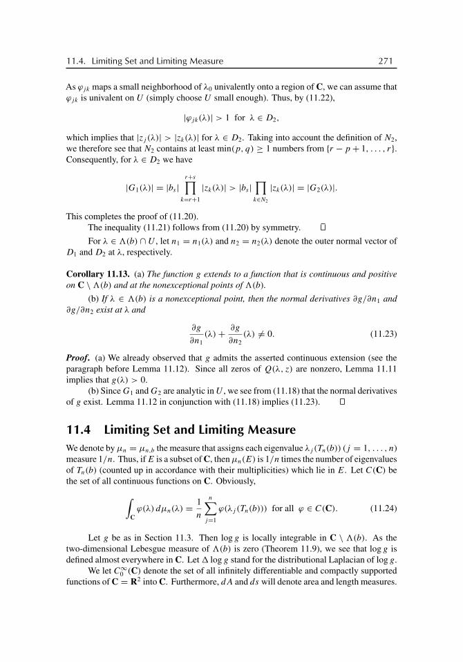
buch72005/10/5page 271

�

�

�

�

�

�

�

�

11.4. Limiting Set and Limiting Measure 271

As ϕjk maps a small neighborhood of λ0 univalently onto a region of C, we can assume thatϕjk is univalent on U (simply choose U small enough). Thus, by (11.22),

|ϕjk(λ)| > 1 for λ ∈ D2,

which implies that |zj (λ)| > |zk(λ)| for λ ∈ D2. Taking into account the definition of N2,we therefore see that N2 contains at least min(p, q) ≥ 1 numbers from {r − p+ 1, . . . , r}.Consequently, for λ ∈ D2 we have

|G1(λ)| = |bs |r+s∏

k=r+1

|zk(λ)| > |bs |∏k∈N2

|zk(λ)| = |G2(λ)|.

This completes the proof of (11.20).The inequality (11.21) follows from (11.20) by symmetry.

For λ ∈ �(b) ∩ U , let n1 = n1(λ) and n2 = n2(λ) denote the outer normal vector ofD1 and D2 at λ, respectively.

Corollary 11.13. (a) The function g extends to a function that is continuous and positiveon C \�(b) and at the nonexceptional points of �(b).

(b) If λ ∈ �(b) is a nonexceptional point, then the normal derivatives ∂g/∂n1 and∂g/∂n2 exist at λ and

∂g

∂n1(λ)+ ∂g

∂n2(λ) �= 0. (11.23)

Proof. (a) We already observed that g admits the asserted continuous extension (see theparagraph before Lemma 11.12). Since all zeros of Q(λ, z) are nonzero, Lemma 11.11implies that g(λ) > 0.

(b) Since G1 and G2 are analytic in U , we see from (11.18) that the normal derivativesof g exist. Lemma 11.12 in conjunction with (11.18) implies (11.23).

11.4 Limiting Set and Limiting MeasureWe denote by μn = μn,b the measure that assigns each eigenvalue λj (Tn(b)) (j = 1, . . . , n)measure 1/n. Thus, if E is a subset of C, then μn(E) is 1/n times the number of eigenvaluesof Tn(b) (counted up in accordance with their multiplicities) which lie in E. Let C(C) bethe set of all continuous functions on C. Obviously,∫

Cϕ(λ) dμn(λ) = 1

n

n∑j=1

ϕ(λj (Tn(b))) for all ϕ ∈ C(C). (11.24)

Let g be as in Section 11.3. Then log g is locally integrable in C \ �(b). As thetwo-dimensional Lebesgue measure of �(b) is zero (Theorem 11.9), we see that log g isdefined almost everywhere in C. Let � log g stand for the distributional Laplacian of log g.

We let C∞0 (C) denote the set of all infinitely differentiable and compactly supportedfunctions of C = R2 into C. Furthermore, dA and ds will denote area and length measures.

buch72005/10/5page 272

�

�

�

�

�

�

�

�


Lemma 11.14. The measures μn converge in the distributional sense to the measure1

2π� log g dA, that is,∫

Cϕ(λ) dμn(λ)→ 1

2π

∫C

log g(λ) �ϕ(λ) dA(λ) (11.25)

for every ϕ ∈ C∞0 .

Proof. Evidently,∫C

log |z− λ| dμn(z) = 1

n

n∑j=1

log |λj (Tn(b))− λ| = log |Dn(b − λ)|1/n.

Thus, by Lemma 11.10, ∫C

log |z− λ| dμn(z)→ log g(λ) (11.26)

uniformly on compact subsets of C \ �(b). It follows that (11.26) is also true in thedistributional sense, whence

1

2π�λ

∫C

log |z− λ| dμn(z)→ 1

2π�λ log g(λ) (11.27)

in the distributional sense. It is well known from potential theory that

1

2π�λ

∫C

log |z− λ| dν(z) = ν(λ)

for every compactly supported finite Borel measure ν. Consequently, (11.27) implies that

μn(λ)→ 1

2π�λ log g(λ)

in the distributional sense, which says that (11.25) holds for all ϕ ∈ C∞0 .

By Corollary 11.13, g and the normal derivatives ∂g/∂n1 and ∂g/∂n2 are well definedat the nonexceptional points of �(b). From Theorem 11.9 we know that �(b) has at mostfinitely many exceptional points.

Lemma 11.15. If ϕ ∈ C∞0 (C), then∫C

log g(λ)(�ϕ)(λ) dA(λ) =∫

�(b)

ϕ(λ)1

g(λ)

∣∣∣∣ ∂g

∂n1(λ)+ ∂g

∂n2(λ)

∣∣∣∣ ds(λ).

Proof. Let λ0 ∈ �(b) be a nonexceptional point and let U be a sufficiently small openneighborhood of λ0. We denote the boundaries of the two connected components D1 andD2 of U \�(b) by ∂D1 and ∂D2, and we put �1 = ∂D1∩�(b), �2 = ∂D2∩�(b). Clearly,�1 and �2 coincide as sets. However, the outer normal n is n1 at the points of �1 and it isn2 at the points of �2 (see Figure 11.2).

buch72005/10/5page 273

�

�

�

�

�

�

�

�

11.4. Limiting Set and Limiting Measure 273

D2

D1

�2

�1

U

�(b)

Figure 11.2. An illustration to the proof.

From Green’s formula,∫�

(u �v − v �u) dA =∫

∂�

(u

∂v

∂n− v

∂u

∂n

)ds, (11.28)

we deduce that∫D1

(log g �ϕ − ϕ � log g) dA =∫

∂D1

(log g

∂ϕ

∂n1− ϕ

∂

∂n1log g

)ds.

By (11.14), log g is harmonic in D1. Thus, � log g = 0, whence∫D1

log g �ϕ dA =∫

∂D1

log g∂ϕ

∂n1ds −

∫∂D1

ϕ∂

∂n1log g ds. (11.29)

Analogously, ∫D2

log g �ϕ dA =∫

∂D2

log g∂ϕ

∂n2ds −

∫∂D2

ϕ∂

∂n2log g ds. (11.30)

Adding (11.29) and (11.30) we obtain∫U

log g �ϕ dA =∫

∂U

log g∂ϕ

∂nds +

∫�1

log g∂ϕ

∂n1ds +

∫�2

log g∂ϕ

∂n2ds

−∫

∂U

ϕ∂

∂nlog g ds −

∫�1

ϕ∂

∂n1log g ds −

∫�2

ϕ∂

∂n2log g ds,

and since

∂ϕ

∂n1+ ∂ϕ

∂n2= 0 and

∂

∂nlog g = 1

g

∂g

∂n,

it follows that ∫U

log g �ϕ dA =∫

∂U

log g∂ϕ

∂nds −

∫∂U

ϕ1

g

∂g

∂nds

−∫

�(b)

ϕ1

g

(∂g

∂n1+ ∂g

∂n2

)ds. (11.31)

buch72005/10/5page 274

�

�

�

�

�

�

�

�


From (11.18) and Lemma 11.12 we infer that

∂g

∂n1< 0 and

∂g

∂n2< 0 on �(b).

Hence

−∫

�(b)

ϕ1

g

(∂g

∂n1+ ∂g

∂n2

)ds =

∫�(b)

ϕ1

g

∣∣∣∣ ∂g

∂n1+ ∂g

∂n2

∣∣∣∣ ds. (11.32)

If supp ϕ ⊂ U , then (11.31) and (11.32) give∫U

log g �ϕ dA =∫

�(b)

ϕ1

g

∣∣∣∣ ∂g

∂n1+ ∂g

∂n2

∣∣∣∣ ds.

Using an appropriate partition of unity it is easily seen that the last equality holds for allϕ ∈ C∞0 (C).

We are now in a position to establish the main results of this chapter.

Theorem 11.16 (Hirschman). The measures dμn converge weakly to the measure that issupported on �(b) and equals

1

2π

1

g

∣∣∣∣ ∂g

∂n1+ ∂g

∂n2

∣∣∣∣ ds on �(b). (11.33)

In other terms,

1

n

n∑j=1

ϕ(λj (Tn(b)))→ 1

2π

∫�(b)

ϕ(λ)1

g(λ)

∣∣∣∣ ∂g

∂n1(λ)+ ∂g

∂n2(λ)

∣∣∣∣ ds(λ) (11.34)

for every ϕ ∈ C(C) with compact support.

Proof. Combining (11.24) and Lemmas 11.14 and 11.15, we see that (11.34) is valid forevery ϕ ∈ C∞0 (C). As C∞0 (C) is dense in the space of all continuous functions with compactsupport, we arrive at the assertion.

Theorem 11.17 (Schmidt and Spitzer). We have �s(b) = �w(b) = �(b).

Proof. To prove that �(b) ⊂ �s(b), pick λ0 ∈ �(b) and let U be any open neighborhoodof λ0. Choose a function ϕ ∈ C∞0 (C) so that supp ϕ ⊂ U and ϕ(λ0) = 1. From Theorem11.16 we get

1

n

n∑j=1

ϕ(λj (Tn(b)))→ 1

2π

∫�(b)

ϕ(λ)1

g(λ)

∣∣∣∣ ∂g

∂n1(λ)+ ∂g

∂n2(λ)

∣∣∣∣ ds(λ) > 0.

buch72005/10/5page 275

�

�

�

�

�

�

�

�

11.5. Connectedness of the Limiting Set 275

As

#{j : λj (Tn(b)) ∈ U}n

= 1

n

n∑j=1

χU(λj (Tn(b))) ≥ 1

n

n∑j=1

ϕ(λj (Tn(b))),

it follows that #{j : λj (Tn(b)) ∈ U} > 0 for all sufficiently large n, which implies thatλ0 ∈ �s(b).

We are left to prove that �w(b) ⊂ �(b). This follows from Corollary 11.2 andTheorem 11.3. We can also argue as follows. Let λ0 /∈ �(b). Then |zr(λ0)| < |zr+1(λ0)|.Since |zr(λ)| and |zr+1(λ)| depend continuously on λ, there is an open neighborhood U of λ0

such that |zr(λ)| < |zr+1(λ)| for all λ ∈ U . By Lemma 11.10, |Dn(b− λ)|1/n → g(λ) > 0for all λ ∈ U . Hence, Dn(b− λ) �= 0 for all sufficiently large n and all λ ∈ U . This showsthat sp Tn(b) ∩ U = ∅ for all sufficiently large n and implies that λ0 /∈ �w(b).

Example 11.18. We already know �(b) in the case where b is a trinomial of the formb(t) = b−1t

−1+ b0+ b1t . One can also describe �(b) explicitly if b is a general trinomial,that is,

b(t) = b−r t−r + b0 + bst

s .

By translation of the plane, we may assume that b0 = 0, and by further rotation and changeof the scale, we may confine ourselves to the case where

b(t) = t−r + t s , r ≥ 1, s ≥ 1, g.c.d.(r, s) = 1.

Schmidt and Spitzer showed that in this case �(b) is the star

�(b) = {ωd : ω = e2πi/(r+s), 0 ≤ d ≤ R

},

where R = (r + s)s−s/(r+s)r−r/(r+s).

The pictures at the top right corners of the beginning pages of the chapters are examplesof symbol curves b(T) and the eigenvalues of T60(b). Figures 11.3 to 11.5 show some moresophisticated examples. These figures were scanned from printouts left by Olga Grudskaya.

11.5 Connectedness of the Limiting Set

Theorem 11.19 (Ullman). If b is a Laurent polynomial, then �(b) is a connected set.

Proof. Assume �(b) is not connected. Then we can find a subset K ⊂ �(b) and a functionϕ ∈ C∞0 (C) such that ϕ|K = 1 and ϕ|�(b) \ K = 0. Moreover, ϕ can be chosen so thatϕ|�1 = 1 and ϕ|�2 = 0 where �1 and �2 are open sets with smooth Jordan boundarieswhich contain K and �(b) \ K , respectively. Let �0 and �3 be open subsets of C whichcontain K and �(b)\K and are contained in the interior of �1 and �2, respectively. We mayassume that �0 and �3 have smooth Jordan boundaries. Finally, put � = C \ (�0 ∪ �3).Abbreviate the limiting measure (11.33) to dμ.

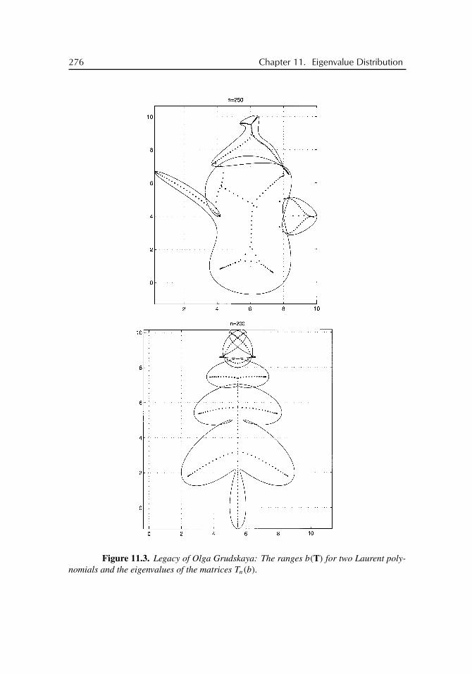
buch72005/10/5page 276

�

�

�

�

�

�

�

�


Figure 11.3. Legacy of Olga Grudskaya: The ranges b(T) for two Laurent poly-nomials and the eigenvalues of the matrices Tn(b).

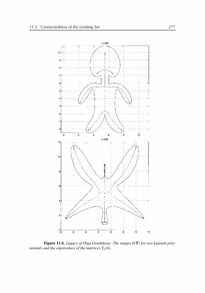
buch72005/10/5page 277

�

�

�

�

�

�

�

�



buch72005/10/5page 278

�

�

�

�

�

�

�

�



buch72005/10/5page 279

�

�

�

�

�

�

�

�


Since μ(�(b)) = 1 and neither K nor �(b) \K can degenerate to a point (Theorem11.9), it follows that

0 < μ(K) < 1. (11.35)

From Lemma 11.15 we obtain

μ(K) =∫

K

dμ =∫

�(b)

ϕ dμ =∫

Clog g �ϕ dA,

and since �ϕ = 0 on �0 and �2, we get

μ(K) =∫

�

log g �ϕ dA.

As � log g = 0 on �, Green’s formula (11.28) implies that

μ(K) =∫

∂�

(log g

∂ϕ

∂n− ϕ

∂ log g

∂n

)ds,

where n is now the outer normal to �. Taking into account that

ϕ | ∂�3 = 0,∂ϕ

∂n

∣∣∣ ∂�3 = 0, ϕ | ∂�0 = 1,∂ϕ

∂n

∣∣∣ ∂�0 = 0,

we get

μ(K) =∫

∂�0

∂ log g

∂nds, (11.36)

where n is now the outer normal to �0. From (11.15) we infer that if λ0 is a point inC \�(b), then the analytic functions Dn+1(b− λ)/Dn(b− λ) converge uniformly in someopen neighborhood of λ0 to some analytic function. Thus, there is an analytic functionG : C \�(b)→ C such that

limn→∞

Dn+1(b − λ)

Dn(b − λ)= G(λ) �= 0

for all λ ∈ C \ �(b). Lemma 11.10 implies that g(λ) = |G(λ)|. Fix a point λ0 ∈ ∂�0

and choose an argument v(λ) = arg G(λ) of G(λ) which is continuous on ∂�0 \ {λ0}. Putu = log g. Since

log G = log |G| + i arg G = u+ iv

is analytic in a neighborhood of ∂�0 \ {λ0}, the Cauchy-Riemann equations give ux = vy

and uy = −vx . Let x = x(t) and y = y(t) (t ∈ (0, 2π)) be a parametrization of of∂�0 \ {λ0}. From (11.36) we now obtain that

μ(K) =∫

∂�0

∂ log g

∂nds =

∫ 2π

0(uxy − uyx) dt

=∫ 2π

0(vxx + vyy) dt =

∫ 2π

0

∂v

∂sds = 1

2πv

∣∣∣∂�0\{λ0}

. (11.37)

buch72005/10/5page 280

�

�

�

�

�

�

�

�


But the number (11.37) is always an integer, which contradicts (11.35).

As the following result shows, �(b) may separate the plane.

Theorem 11.20. Let b(t) = μ+ t−r (t − α)r(t − β)r , where μ, α, β are complex numbersand αβ �= 0. If r = 1 or r = 2, then C \�(b) is connected. If r ≥ 3, then C \�(b) has atmost [(r + 1)/2] components (including the unbounded component), and for each naturalnumber j between 1 and [(r + 1)/2] there exist α and β such that C \�(b) has exactly j

components.

Proof. Put a(t) = t−1(t−α)(t −β). The curve a(T) is an ellipse with the foci−(α+β)±2√

αβ and �(a) is the line segment between the foci. Obviously,

b(t) = μ+ (a(t))r .

We claim that

�(b) = μ+ (�(a))r . (11.38)

To prove our claim, we assume for the sake of definiteness that a(t) traces out a(T) coun-terclockwise as t moves around T counterclockwise. Notice that b� = μ + ar

� for all� ∈ (0,∞).

Pick λ ∈ �(a). Then λ ∈ sp T (a�) for all � ∈ (0,∞) due to Theorem 11.3. Putω = e2πi/r . If ωkλ ∈ a�(T) for some k ∈ {1, . . . , r}, then

μ+ λr = μ+ (ωkλ)r ∈ b�(T)

and hence μ+ λr ∈ sp T (b�). Now assume that ωkλ /∈ a�(T) for all k ∈ {1, . . . , r}. Sinceλ ∈ sp T (a�), it follows that wind (a� − λ) = 1. As b� − μ− λr = ar

� − λr , we have

wind (b� − μ− λr) = windr∏

k=1

(a� − ωkλ) =r∑

k=1

wind (a� − ωkλ),

and as wind (a� − ωkλ) is either 0 or 1, we conclude that wind (b� − μ − λr) ≥ 1. Con-sequently, μ + λr ∈ sp T (b�). From Theorem 11.3 we now obtain the inclusion “⊃” in(11.38). To verify the reverse inclusion, let � ∈ C \ {0} be any number such that �2 = αβ.Then a�(T) = �(a). It results that b�(T) = μ+ (�(a))r , and as wind (b� − ζ ) = 0 for allζ /∈ b�(T), we see that sp T (b�) = μ+ (�(a))r . Since⋂

�∈C\{0}sp T (b�) =

⋂�∈(0,∞)

sp T (b�),

we infer from Theorem 11.3 that �(b) ⊂ sp T (b�) = μ+ (�(a))r , which is the inclusion“⊂” of (11.38).

Since neither a line segment nor the square of a line segment does separate the plane,we obtain from equality (11.38) the assertion for r = 1 and r = 2. Combining (11.38) withthe fact that �(a) is a line segment, one can easily see that the set C \ �(b) has at most[(r+1)/2] components and that each number of components between 1 and [(r+1)/2] canindeed be realized (for example, we get exactly [(r+1)/2] components if |μ−(α+β)| > 0is sufficiently small and |αβ| is sufficiently large.

buch72005/10/5page 281

�

�

�

�

�

�

�

�

Exercises 281

Exercises

1. Gershgorin’s theorem states that if An = (aij ) is an n× n matrix and

R′i (An) :=⎛⎝ n∑

j=1

|aij |⎞⎠− |aii |,

then

sp An ⊂n⋃

i=1

{λ ∈ C : |λ− aii | ≤ R′i (An)}.

Show that in the case of large Toeplitz band matrices this theorem amounts to thetrivial estimate rad Tn(b) ≤ ‖b‖W .

2. Let b ∈ P and suppose R(b) ⊂ R. Let further {a1, a2, a3, . . . } be a convergentsequence of real numbers. Put

An = Tn(b)+ diag (a1, . . . , an), A = T (b)+ diag (a1, a2, . . . ).

Show that


n→∞sp An = sp A.

3. Let a ∈ P and let Hn(a) = PnH(a)Pn|Im Pn.

(a) Show that �(Hn(a)) and sp Hn(a) converge to �(H(a)) and sp H(a), respectively,in the Hausdorff metric.

(b) Show that �(H(a)) and sp H(a) are finite sets containing the origin.

(c) Prove that

limn→∞

1

n

n∑j=1

ϕ(σj (Hn(a))) = limn→∞

1

n

n∑j=1

ϕ(λj (Hn(a))) = ϕ(0)

for every measurable function ϕ that is continuous at the origin.

4. Let b be a Laurent polynomial.

(a) Show that sp Tn(b) ⊂ convR(b) for all n ≥ 1.

(b) Prove that

limn→∞

1

n

n∑j=1

ϕ(λj (Tn(b))) = 1

2π

∫ 2π

0ϕ(eiθ ) dθ (11.39)

for every function ϕ that is analytic in a disk containing convR(b).

buch72005/10/5page 282

�

�

�

�

�

�

�

�


(c) Let � ⊂ C be an open set such that convR(b) ⊂ �. Prove that (11.39) is true forevery harmonic function ϕ on �.

(d) What does (11.39) say for b(t) = b0 + b1(t)?

(e) Let � be an open set in the plane and ϕ ∈ C(�). Prove that if (11.39) is true forevery b with convR(b) ⊂ �, then ϕ is harmonic on �.

5. Let a, b ∈ P and consider An = Tn(b) + Hn(a). Fix an open subset � of C thatcontains sp T (b) ∪ sp (T (b)+H(a)).

(a) Show that sp An ⊂ � for all sufficiently large n.

(b) Show that

limn→∞

1

n

⎡⎣ n∑j=1

p(λj (An))−n∑

j=1

p(λj (Tn(b)))

⎤⎦= lim

n→∞1

ntr [p(An)− p(Tn(b))] = 0

for every polynomial p ∈ P+.

(c) Prove that if ϕ is harmonic in �, then

limn→∞

1

n

n∑j=1

ϕ(λj (An)) = 1

2π

∫�(b)

ϕ(λ)dμ(λ),

where dμ is the measure (11.33).

6. Do the mass centers of the sets �(b) and sp T (b) always coincide?

7. Compute the determinant and the eigenvalues of the Toeplitz matrix

An =

⎛⎜⎜⎜⎝c + 1 a . . . an−1

a−1 c + 1 . . . an−2

......

. . ....

a−(n−1) a−(n−2) . . . c + 1

⎞⎟⎟⎟⎠ .

Notes

Sections 11.1 to 11.4 are based on the pioneering papers on this topic, Schmidt and Spitzer[243] and Hirschman [165], and on some significant improvements of the original proofsthat were introduced by Widom [296], [297]. Theorem 11.19 was established in [286].

Exercise 3 is of course easy. For the spectral distribution of more general Hankelmatrices we refer to Fasino and Tilli’s papers [115] and [116]. Exercise 4 is a result of Tilli[264]. The analogue of Exercise 5 for the singular values is in [116], for example. The resultof Exercise 5 can probably be generalized to a broader class of test functions ϕ. Exercise 7is from Sakhnovich’s paper [241].

buch72005/10/5page 283

�

�

�

�

�

�

�

�

Notes 283

Further results: limiting sets separating the plane. For a long time it had been an openquestion whether the set �(b) may separate the plane. In 1992, Anselone and Sloan [6]studied the truncated Wiener-Hopf operator

(Aτf )(x) = 2∫ x

0e−(x−t)f (t)dt +

∫ τ

x

ex−t f (t)dt (0 < x < τ)

on L2(0, τ ). They were interested in the set � of all λ ∈ C such that λ = lim λn with λn ∈sp Aτn

and τn →∞, and on the basis of numerical experiments, they conjectured that � is theunion of the circle {λ ∈ C : |λ−1/12| = 1/12} and the line segment [3/2−√2, 3/2+√2 ].Note that this set separates the plane. The symbol of the corresponding “infinite” Wiener-Hopf operator

(Af )(x) = 2∫ x

0e−(x−t)f (t)dt +

∫ ∞

x

ex−t f (t)dt (0 < x <∞)

on L2(0,∞) is the Fourier transform of the kernel,

a(x) =∫ 0

−∞eixt etdt +

∫ ∞

0eixt · 2e−t dt = 3+ ix

1+ x2(x ∈ R := R ∪ {∞}).

This is a rational function and a(R) is an ellipse. In a sense, Anselone and Sloan’s conjectureanswered the continuous analogue on the question whether �(b) may separate the plane inthe negative. In [72], the continuous analogue of Theorem 11.17 was established, and thisresult implied that the conjecture of Anselone and Sloan was true. Thus, it was Wiener-Hopfoperators with rational symbols that showed us for the first time a limiting set � for whichC \� is disconnected (see Figure 11.6).

0 1 2 3−1.5

−1

−0.5

0

0.5

1

1.5

−0.1 0 0.1 0.2 0.3

−0.15

−0.1

−0.05

0

0.05

0.1

0.15

0.2

Figure 11.6. The ellipse a(R) and the limiting set � on the left and a zoom in onthe right.

In the context of Toeplitz band matrices, symbols b for which �(b) separates theplane were detected numerically in [20] (Figure 5.3(c)) and [71] (lower left picture of

buch72005/10/5page 284

�

�

�

�

�

�

�

�


Figure 38, the “smiling shark”). The picture on the first page of this chapter also shows adisconnected set C \�(b); the corresponding symbol is b(t) = t−3 + 0.99 t−2 + 0.1 t2 −0.44 t3. Theorem 11.20, which is a first “analytic” result in this direction, is from our paper[50].

Further results: dense Toeplitz matrices. The sets �s(b) and �w(b) can be defined forToeplitz matrices T (b) with arbitrary symbols b, but for general symbols b things remainmysterious. In the case of rational symbols, the limiting sets were characterized by K. M.Day [97], [98] (the result is also cited in [71, Section 5.9], and for the underlying determinantformula see also [32]).

For certain classes of continuous or piecewise continuous symbols b, the asymptoticeigenvalue distribution of Tn(b) can be described by formulas of the Szegö type. These saythat if λ

(n)1 , . . . , λ(n)

n are the eigenvalues of Tn(b), then

limn→∞

1

n

n∑j=1

ϕ(λ(n)j ) = 1

2π

∫ 2π

0ϕ(b(eiθ ))dθ (11.40)

for every continuous function ϕ : C → R with compact support (see [15], [71], [265],[296], [297] for details). Notice that (11.40) implies that, up to o(n) possible outliers, theeigenvalues cluster along the (essential) range b(T) of the symbol but that (11.40) does nottell us whether the possible o(n) outliers produce additional pieces of �w(b).

In order to find �w(b), one can try computing sp Tn(b) for some large values of n nu-merically, having hopes that the result is a more or less good approximation to �w(b). Thisworks for rational symbols and, in general, also for the symbols for which (11.40) holds.Another possibility of determining �w(b) is to approximate b by a Laurent polynomial bn,surmising that �w(bn) is close to �w(b). This approach fails for piecewise continuoussymbols, which should not come as a surprise, since a properly piecewise continuous func-tion can never be approximated uniformly by Laurent polynomials as closely as desired.Unexpectedly, this approach does in general also not work for continuous symbols. This isa consequence of the main result of [51], which shows that the asymptotic spectrum �w(·)is discontinuous on the space of continuous symbols. The result of [51] is as follows: Thereexist b ∈ W such that �w(Snb) does not converge to �w(b) in the Hausdorff metric. HereSnb denotes the nth partial sum of the Fourier series (see Section 5.3).

Figures 11.7 and 11.8, which are from [51] and were produced by Olga Grudskaya,convincingly illustrate what happens. The symbol b is

b(t) = t−1(33− (t + t2)(1− t2)3/4).

This is a continuous function which is piecewise C∞ but not C∞. The matrix T (b) is a lowerHessenberg matrix. The results of Widom [296] imply that (11.40) is valid, that is, we expectthat the eigenvalues of Tn(b) cluster along the range b(T) of the symbol. The two picturesof Figure 11.7 show the range b(T) and the eigenvalues of Tm(b) for m = 128 (left) andm = 512 (right). In Figure 11.8, we plot the eigenvalues of T128(Snb) for n = 4, 6, 8, 12.These eigenvalue distributions mimic the sets �w(Snb) sufficiently well, and it is clearlyseen that �w(Sna) grows like a rampant tree that in the n→∞ limit has nothing in commonwith �w(b).

buch72005/10/5page 285

�

�

�

�

�

�

�

�

Notes 285

Figure 11.7. The range b(T) and the eigenvalues of T128(b) (left) and T512(b) (right).

Figure 11.8. The range b(T) and the eigenvalues of T128(Snb) for the valuesn = 4, 6, 8, 12.

buch72005/10/5page 286

�

�

�

�

�

�

�

�

buch72005/10/5page 287

�

�

�

�

�

�

�

�

Chapter 12

Eigenvectorsand Pseudomodes

In previous chapters, we studied the asymptotic behavior of eigenvalues and pseudoeigen-values (= points in the pseudospectrum) of large Toeplitz matrices. This chapter concernsasymptotic results on eigenvectors and pseudomodes (= pseudoeigenvectors). We will inparticular point out that there are striking differences between the Toeplitz and circulantcases.

12.1 Tridiagonal Circulant and Toeplitz MatricesLet b(t) = t+α2t−1. In Sections 2.1 and 2.2 we found explicit formulas for the eigenvectorsof Cn(b) and Tn(b). The purpose of this section is to give the reader some delight with afew pictures that can be easily produced with MATLAB.

Let n ≥ 3. We know from Proposition 2.1 that the eigenvectors of Cn(b) normalizedto �2 norm 1 are x1, . . . , xn with

xj = 1√n

(1, ω j−1

n , ω 2(j−1)n , . . . , ω (n−1)(j−1)

n

), (12.1)

where ωn = e2πi/n. Theorem 2.4 tells us that after normalization to the �2 norm 1 theeigenvectors of Tn(b) are x1, . . . , xn with

xj = cn(α)

(1

αsin

πj

n+ 1,

(1

α

)2

sin2πj

n+ 1, . . . ,

(1

α

)n

sinnπj

n+ 1

), (12.2)

where cn(α) is the normalization constant. Note first of all that (12.1) is independent of b,while (12.2) depends on b. A second immediate observation is that the absolute values ofthe components of the eigenvectors (12.1) are constant, whereas those of (12.2) are localizedin the left for |α| > 1 and in the right for |α| < 1.

The eigenvectors x1, . . . , xn form a basis in Cn. When identifying Cn with R2n, theseeigenvectors deliver the basis

(Re x1, Im x1), . . . , (Re xn, Im xn), (−Im x1, Re x1), . . . , (−Im xn, Re xn) (12.3)

287

buch72005/10/5page 288

�

�

�

�

�

�

�

�

288 Chapter 12. Eigenvectors and Pseudomodes

in R2n. Notice that Im xj = 0 for all j in the Toeplitz case provided α is real.The second half of the basis (12.3) clearly mimics the first half. In Figure 12.1 we

plotted the 10 vectors of the first halves of the bases (12.3) for C10(b) and T10(b) withα = 3/2.

We arrange the 2n vectors (12.3) to a (2n)×(2n) matrix and denote this matrix by ECn

in the circulant case and by ETn(α) in the Toeplitz case. Figure 12.2 shows pseudocolorplots of the matrices EC30 and ET30(3/2). A gray point indicates a matrix entry near zero,dark points stand for positive entries, and light points represent negative ones. The rightpicture of Figure 12.1 and especially the bottom picture of Figure 12.2 show that (12.3) is avery ill-conditioned basis in the Toeplitz case. Finally, Figures 12.3 and 12.4 depict surfaceplots of the matrices EC30 and ET30(3/2) from two different viewpoints. Whatever insightsthese two figures might provide, they show us at least the bizarre difference between twoworlds.

12.2 Eigenvectors of Triangular and Tridiagonal MatricesWe now turn to the eigenvectors of general banded Toeplitz matrices. Letb(t) =∑s

j=−r bj tj

be a Laurent polynomial. As in Chapter 11, we write

b(t)− λ = t−rbs(t − z1(λ)) . . . (t − zr+s(λ)), |z1(λ)| ≤ · · · ≤ |zr+s(λ)|. (12.4)

The system Tn(b − λ)xn = 0 (xn ∈ Cn) is a difference equation with constant coefficientsand r+s boundary conditions. Analogously, the equation T (b−λ)x0 = 0 (x0 ∈ �2) is a dif-ference equation that has constant coefficients, and the constraints are s boundary conditionsand the requirement that x0 be in �2. Thus, once λ is an eigenvalue, the eigenvectors canbe expressed in terms of the zeros z1(λ), . . . , zr+s(λ) of (12.4) and certain coefficients thatcan be determined from the boundary constraints. The resulting formulas are neverthelessvery complicated and inappropriate for answering the question we are interested in here ina straightforward fashion. Trench [278] derived simpler equations for the eigenvalues ofTn(b) and constructed simpler formulas for the eigenvectors (see Exercise 2). Again, theseformulas cannot be immediately employed in order to see the asymptotic behavior of theeigenvectors.

An interesting result on the eigenvectors was established by Zamarashkin and Tyrtysh-nikov [301], [302]. They proved that the eigenvectors of Tn(b) are asymptotically distributedas the columns of the Hermitian adjoint of the Fourier matrix,

F ∗n =

1√n

(e−i 2πn

jk)n−1j,k=0 =: (col(n)

1 , . . . , col(n)n ),

in the following sense: For each ε > 0, the number of integers k ∈ {1, . . . , n} for whichminλ ‖Tn(b − λ) col(n)

k ‖2 > ε is o(n) as n→∞.We here consider an entirely different question. Take a λn in sp Tn(b) for each n ≥ 1

and suppose the points λn converge to some point λ. Clearly, λ belongs to the limiting set�(b) studied in Chapter 11. Conversely, given any λ ∈ �(b), we can find λn ∈ sp Tn(b)

such that λn → λ. If λ is an eigenvalue of T (b), are the eigenvectors of Tn(b) correspondingto the eigenvalues λn related to the eigenvectors of T (b) corresponding to λ? What can besaid about the eigenvectors of Tn(b) for λn in the case where λ is not an eigenvalue of T (b)?

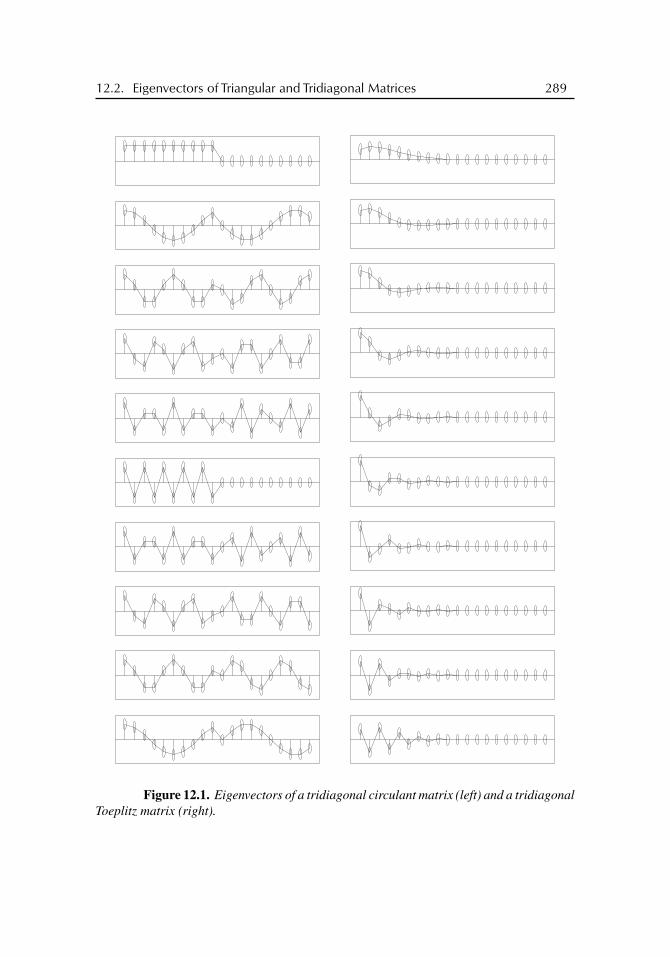
buch72005/10/5page 289

�

�

�

�

�

�

�

�

12.2. Eigenvectors of Triangular and Tridiagonal Matrices 289

Figure 12.1. Eigenvectors of a tridiagonal circulant matrix (left) and a tridiagonalToeplitz matrix (right).

buch72005/10/5page 290

�

�

�

�

�

�

�

�


5 10 15 20 25 30 35 40 45 50 55 60

5

10

15

20

25

30

35

40

45

50

55

60

5 10 15 20 25 30 35 40 45 50 55 60

5

10

15

20

25

30

35

40

45

50

55

60

Figure 12.2. A pseudocolor plot of the real eigenvector basis of a tridiagonalcirculant matrix (top) and a tridiagonal Toeplitz matrix (bottom).

buch72005/10/5page 291

�

�

�

�

�

�

�

�


Eigenvectors of infinite Toeplitz matrices were investigated in Section 1.8. We repeatProposition 1.20 in slightly modified form.

Proposition 12.1. Let λ ∈ sp T (b) and suppose that λ /∈ b(T). The point λ is an eigenvalueofT (b)as an operator on�2 if and only if wind (b, λ) = −m < 0. In that case dimKer T (b−λ) = m and Ker T (b − λ) = lin{x0, V x0, . . . , V

m−1x0}, where V is the shift operator

V : �2 → �2, {w1, w2, . . . } �→ {0, w1, w2, . . . }and x0 = {x(0)

k }∞k=1 is an exponentially decaying sequence with x(0)1 = 1.

Proof. The proof of Proposition 1.20 gives

Ker T (b − λ) = lin {T (b−1+ )e0, . . . , T (b−1

+ )em−1}.We may think of T (b−1

+ )ej as the j th column of the lower-triangular Toeplitz matrix T (b−1+ ).

As the 0th Fourier coefficient of b−1+ may be assumed to be 1 and the Fourier coefficients of

b−1+ decay exponentially, we get all assertions.

Triangular Toeplitz matrices. Suppose b(t) = b0 + b−1t−1 + · · · + b−r t

−r with r ≥ 1and b−r �= 0. The matrix T (b) is upper triangular. It is clear that sp Tn(b) = {b0} for alln and hence �(b) = {b0}. We assume that b0 /∈ b(T). Let b−1 = · · · = b−m0+1 = 0 andb−m0 �= 0. Then

b(t)− b0 = b−m0 t−r (t − δ1) . . . (t − δp)(t − μ1) . . . (t − μq),

where |δk| < 1 and |μk| > 1 for all k. Since p + q = r −m0, we get

wind (b, b0) = −r + p = −m0 − q ≤ −m0 ≤ −1. (12.5)

Thus, by Proposition 12.1, Ker T (b− b0) has the dimension m0+ q and from the proofs ofPropositions 1.20 and 12.1 we infer that

Ker T (b − b0) = lin {T (b−1+ )e1, . . . , T (b−1

+ )em0+q}with

b−1+ (t) =

q∏k=1

(1+ t

μ1+ t2

μ21

+ · · ·)

.

On the other hand, it is easily seen that Ker Tn(b − b0) = lin {e1, . . . , em0}. Consequently,in general Ker Tn(b−b0) and Ker T (b−b0) are in no way related. If b−1 �= 0 (⇔ m0 = 1),which is the generic case, then Ker Tn(b−b0) is spanned by e1. If, in addition, wind (b, b0) =−1, then q = 0 and hence Ker T (b− b0) is also spanned by e1. This is in accordance withTheorem 12.3, which will be proved below. However, in the case where b−1 �= 0 andwind (b, b0) ≤ −2, no eigenvector of T (b) that is outside lin {e1} can be approximated byeigenvectors of Tn(b).

If b(t) = b0 + b1t + · · · + bsts (s ≥ 1, bs �= 0), then T (b) is lower triangular.

Again sp Tn(b) = {b0} for all values of n and �(b) = {b0}. From (12.5) we obtain that

buch72005/10/5page 292

�

�

�

�

�

�

�

�


010

2030

4050

60

0

10

20

30

40

50

60–0.2

–0.15

–0.1

–0.05

0

0.05

0.1

0.15

0.2

010

2030

4050

60

0

10

20

30

40

50

60–1

–0.5

0

0.5

1

Figure 12.3. A surface plot of the real eigenvector basis of a tridiagonal circulantmatrix (top) and a tridiagonal Toeplitz matrix (bottom).

buch72005/10/5page 293

�

�

�

�

�

�

�

�


010

2030

4050

60

0

20

40

60

–0.2

–0.15

–0.1

–0.05

0

0.05

0.1

0.15

0.2

010

2030

4050

60

0

20

40

60

–1

–0.5

0

0.5

1

Figure 12.4. Another view at the surface plots of Figure 12.3.

buch72005/10/5page 294

�

�

�

�

�

�

�

�


wind (b, b0) = −wind (b, b0) ≥ 1, and hence Ker T (b−b0) = {0} by virtue of Proposition12.1. If b1 = · · · = bm0−1 = 0 and bm0 �= 0, then Ker Tn(b − b0) = lin {en, . . . , en−m0+1}.Tridiagonal Toeplitz matrices. Let b(t) = b−1t

−1 + b0 + b1t . Fix one of the two valuesof√

b−1/b1 and denote it by α. Define√

b1b−1 as b1α. By Theorem 2.4, the eigenvaluesof Tn(b) are

λj = b0 + 2√

b1b−1 cosπj

n+ 1(j = 1, . . . , n),

and an eigenvector for λj is xj,n = (x(n)j,k )

nk=1 with

x(n)j,k =

(1

α

)k−1

sinkπj

n+ 1/ sin

πj

n+ 1(k = 1, . . . , n).

It follows that �(b) is the line segment [ b0 − 2√

b1b−1, b0 + 2√

b1b−1 ]. The range b(T)

is an ellipse with the foci b0± 2√

b1b−1 for |α| �= 1 and the line segment �(b) for |α| = 1.Consequently, the spectrum of T (b) consists of the points on the ellipse and in its interiorfor |α| �= 1 and coincides with the line segment �(b) for |α| = 1. If |α| < 1, thenwind (b, λ) = 1 for all λ ∈ �(b), while if |α| > 1, we have wind (b, λ) = −1 for allλ ∈ �(b).

Now pick a point λ = b0 + 2√

b1b−1 cos θ ∈ �(b) (θ ∈ [0, π ]) and chose anyjn ∈ {1, . . . , n} such that πjn/(n+ 1)→ θ as n→∞. Then

λn := b0 + 2√

b1b−1 cosπjn

n+ 1∈ sp Tn(b)

and λn → λ. For the kth component of the eigenvector xn := xjn,n we obtain

x(n)k =

(1

α

)k−1

sinkπjn

n+ 1/ sin

πjn

n+ 1→

(1

α

)k−1 sin kθ

sin θ=: x(0)

k as n→∞,

with the convention that sin(kθ) / sin θ = k in the cases θ = 0 and θ = π . Put x0 ={x(0)

k }∞k=1. If |α| ≤ 1, then x0 /∈ �2, and T (b) is known to have no eigenvalues in this case(Proposition 12.1 for |α| < 1 and Theorem 1.31 for |α| = 1). However, if |α| > 1, thenx0 ∈ �2, Ker T (b − λ) is one dimensional and x0 is an eigenvector of T (b) for λ. Clearly,if |α| > 1, then xn converges to x0 not only componentwise but even in �2.

The conclusion is as follows. Let λ ∈ �(b), λn ∈ sp Tn(b), and λn → λ. The matrixTn(b) has exactly one eigenvector xn for λn satisfying the normalization condition x

(n)1 = 1.

If λ is an eigenvalue of T (b) and x0 is an eigenvector for λ, then x0 can be normalized so thatx

(0)1 = 1. In the case where λ is an eigenvalue of T (b), the vectors xn converge to x0 in �2,

but in the case where λ is not an eigenvalue of T (b), the vectors xn converge componentwiseto some vector x0 that does not belong to the space �2.

12.3 Asymptotics of EigenvectorsNow take λ ∈ C \ b(T) and suppose wind (b, λ) = −m < 0. We then can write b − λ =χ−mc, where χk(t) := tk (t ∈ T) and c is a Laurent polynomial without zeros on T and

buch72005/10/5page 295

�

�

�

�

�

�

�

�

12.3. Asymptotics of Eigenvectors 295

with wind (c, 0) = 0. Let c(t) = ∑j cj t

j (t ∈ T). Since 0 /∈ c(T) and wind (c, 0) = 0, itfollows that the operator T (c) is invertible on �2, that the matrices Tn(c) are invertible forall sufficiently large n, and that T −1

n (c)Pn converges strongly to T −1(c) on �2 (Corollaries1.11 and 3.8).

Lemma 12.2. Let λ ∈ sp Tn(b). Suppose λ /∈ b(T) and wind (b, λ) = −m < 0. A vectorx = (xj )

nj=1 belongs to Ker Tn(b − λ) if and only if

−Tn(c)

⎛⎜⎜⎜⎜⎜⎜⎜⎜⎜⎜⎝

xm+1

xm+2...

xn

0...

0

⎞⎟⎟⎟⎟⎟⎟⎟⎟⎟⎟⎠= xm

⎛⎜⎜⎜⎝c1

c2...

cn

⎞⎟⎟⎟⎠+ · · · + x1

⎛⎜⎜⎜⎝cm

cm+1...

cm+n−1

⎞⎟⎟⎟⎠ . (12.6)

Proof. We have b − λ = cχ−m and hence, by Proposition 3.10,

Tn(b − λ) = Tn(cχ−m) = Tn(c)Tn(χ−m)+ PnH(c)H(χm)Pn.

It follows that Tn(b − λ)x = 0 if and only if

−Tn(c)Tn(χ−m)x = PnH(c)H(χm)Pnx,

which is the same as (12.6).

The following result shows that things are remarkably nice in the case m = 1.

Theorem 12.3. Let λ ∈ �(b), λn ∈ sp Tn(b), λn → λ. Suppose that λ /∈ b(T) and thatwind (b, λ) = −1. Then there exist n0 ∈ N, xn ∈ Cn (n ≥ n0), and x0 ∈ �2 such thatx

(n)1 = 1 and

Ker Tn(b − λn) = lin {xn}, Ker T (b − λ) = lin {x0}, xn → x0 in �2.

Proof. We have b − λ = χ−1c with c as above and

b − λn = b − λ+ λ− λn = χ−1(c + (λ− λn)χ1) =: χ−1(c + δnχ1).

Since Tn(c + δnχ1) = Tn(c) [I + δnT−1n (c)Tn(χ1)] and ‖δnT

−1n (c)Tn(χ1)‖ ≤ 1/2 for all

n large enough, we see that Tn(c + δnχ1) is invertible for all sufficiently large n and thatT −1

n (c + δnχ1)Pn converges strongly to T −1(c) on �2.Lemma 12.2 shows that xn = (x

(n)j )nj=1 is in Ker Tn(b − λn) if and only if⎛⎜⎜⎜⎜⎜⎝

x(n)2

x(n)3...

x(n)n

0

⎞⎟⎟⎟⎟⎟⎠ = −T −1n (c + δnχ1) x

(n)1

⎛⎜⎜⎜⎝c1 + δn

c2...

cn

⎞⎟⎟⎟⎠ . (12.7)

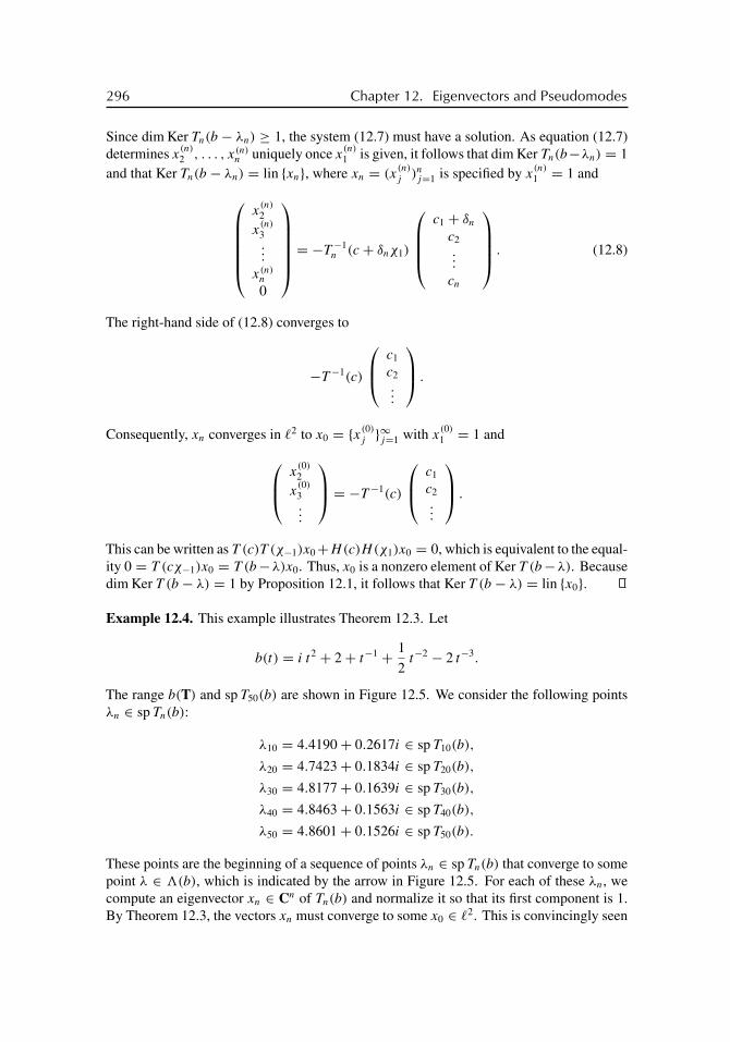
buch72005/10/5page 296

�

�

�

�

�

�

�

�


Since dim Ker Tn(b − λn) ≥ 1, the system (12.7) must have a solution. As equation (12.7)determines x

(n)2 , . . . , x(n)

n uniquely once x(n)1 is given, it follows that dim Ker Tn(b−λn) = 1

and that Ker Tn(b − λn) = lin {xn}, where xn = (x(n)j )nj=1 is specified by x

(n)1 = 1 and⎛⎜⎜⎜⎜⎜⎝

x(n)2

x(n)3...

x(n)n

0

⎞⎟⎟⎟⎟⎟⎠ = −T −1n (c + δnχ1)

⎛⎜⎜⎜⎝c1 + δn

c2...

cn

⎞⎟⎟⎟⎠ . (12.8)

The right-hand side of (12.8) converges to

−T −1(c)

⎛⎜⎝ c1

c2...

⎞⎟⎠ .

Consequently, xn converges in �2 to x0 = {x(0)j }∞j=1 with x

(0)1 = 1 and⎛⎜⎝ x

(0)2

x(0)3...

⎞⎟⎠ = −T −1(c)

⎛⎜⎝ c1

c2...

⎞⎟⎠ .

This can be written as T (c)T (χ−1)x0+H(c)H(χ1)x0 = 0, which is equivalent to the equal-ity 0 = T (cχ−1)x0 = T (b−λ)x0. Thus, x0 is a nonzero element of Ker T (b−λ). Becausedim Ker T (b − λ) = 1 by Proposition 12.1, it follows that Ker T (b − λ) = lin {x0}.

Example 12.4. This example illustrates Theorem 12.3. Let

b(t) = i t2 + 2+ t−1 + 1

2t−2 − 2 t−3.

The range b(T) and sp T50(b) are shown in Figure 12.5. We consider the following pointsλn ∈ sp Tn(b):

λ10 = 4.4190+ 0.2617i ∈ sp T10(b),

λ20 = 4.7423+ 0.1834i ∈ sp T20(b),

λ30 = 4.8177+ 0.1639i ∈ sp T30(b),

λ40 = 4.8463+ 0.1563i ∈ sp T40(b),

λ50 = 4.8601+ 0.1526i ∈ sp T50(b).

These points are the beginning of a sequence of points λn ∈ sp Tn(b) that converge to somepoint λ ∈ �(b), which is indicated by the arrow in Figure 12.5. For each of these λn, wecompute an eigenvector xn ∈ Cn of Tn(b) and normalize it so that its first component is 1.By Theorem 12.3, the vectors xn must converge to some x0 ∈ �2. This is convincingly seen

buch72005/10/5page 297

�

�

�

�

�

�

�

�


−2 0 2 4 6−5

−4

−3

−2

−1

0

1

2

3

Figure 12.5. The range b(T) and the 50 eigenvalues of T50(b) for the symbolof Example 12.4. The arrow points to a point in �(b) that is approximated by pointsλn ∈ sp Tn(b).

in Figure 12.6, which shows the real part of xn in the left column and the imaginary part ofxn in the right. The top row corresponds to n = 10, the bottom row to n = 50.

We now turn to the case where wind (b, λ) = −m ≤ −2. We will then prove thatgenerically the kernels of Tn(b − λn) are one dimensional, Tn(b − λn) = lin {xn}, that thevectors xn ∈ Cn converge to some x0 ∈ Ker T (b− λ), and that the limits x0 correspondingto different choices of the sequence λn → λ all belong to a single one-dimensional subspaceof Ker T (b − λ).

Given λ ∈ �(b), we write the factorization (12.4) now in the form

b(t)− λ = bst−r (t − z

(0)1 ) . . . (t − z

(0)r+s), |z(0)

1 | ≤ · · · ≤ |z(0)r+s |.

Since �(b) = {λ ∈ C : |zr(λ)| = |zr+1(λ)|} by virtue of Theorem 11.17, the point λ

belongs to �(b) if and only if |z(0)r | = |z(0)

r+1|.

Theorem 12.5. Let r ≥ 1, s ≥ 1, λ ∈ �(b), λ /∈ b(T), λn ∈ sp Tn(b), and λn → λ.Suppose |z(0)

r−1| < |z(0)r |. Then, for all sufficiently large n,

Ker Tn(b − λn) = lin {xn}with certain xn = (x

(n)j )nj=1 ∈ Cn satisfying x

(n)1 = 1. The limits

x(0)k = lim

n→∞ x(n)k

exist for all k ≥ 2. If wind (b, λ) ≤ −1, then

{1, x(0)2 , x

(0)3 , . . . } ∈ Ker T (b − λ),

while if wind (b, λ) ≥ 0, we have Ker T (b − λ) = {0} and

{1, x(0)2 , x

(0)3 , . . . } /∈ �2.

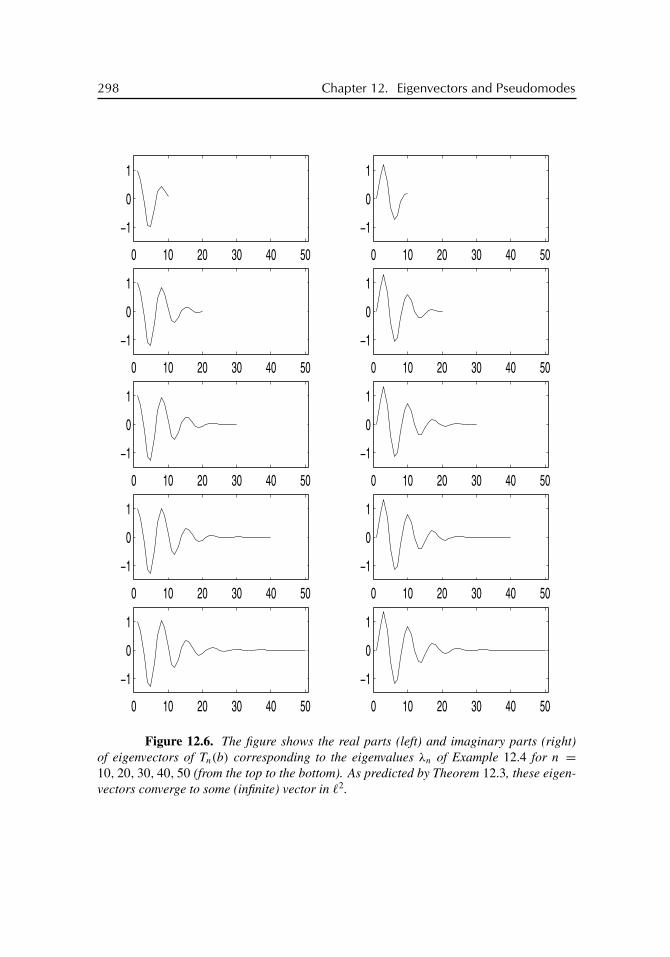
buch72005/10/5page 298

�

�

�

�

�

�

�

�


0 10 20 30 40 50

−1

0

1

0 10 20 30 40 50

−1

0

1

0 10 20 30 40 50

−1

0

1

0 10 20 30 40 50

−1

0

1

0 10 20 30 40 50

−1

0

1

0 10 20 30 40 50

−1

0

1

0 10 20 30 40 50

−1

0

1

0 10 20 30 40 50

−1

0

1

0 10 20 30 40 50

−1

0

1

0 10 20 30 40 50

−1

0

1

Figure 12.6. The figure shows the real parts (left) and imaginary parts (right)of eigenvectors of Tn(b) corresponding to the eigenvalues λn of Example 12.4 for n =10, 20, 30, 40, 50 (from the top to the bottom). As predicted by Theorem 12.3, these eigen-vectors converge to some (infinite) vector in �2.

buch72005/10/5page 299

�

�

�

�

�

�

�

�


Proof. Recall the definition of b� given in Section 11.1. The key observation, alreadyused in Chapter 11, is the identity Tn(b� − λn) = D�Tn(b − λn)D

−1� , where D� =

diag (1, �, . . . , �n−1). This identity implies that

sp Tn(b) = sp Tn(b�), Ker Tn(b − λn) = D−1� Ker Tn(b� − λn). (12.9)

We have

b�(t)− λ = bs�−r t−r (�t − z

(0)1 ) . . . (�t − z

(0)r+s)

= bs(−z(0)1 ) . . . (−z

(0)r+s)�

−r t−r

(1− �t

z(0)1

). . .

(1− �t

z(0)r+s

).

By assumption, we can choose a � ∈ (0,∞) such that

�

|z(0)1 |

≥ · · · ≥ �

|z(0)r−1|

> 1 >�

|z(0)r |

≥ · · · ≥ �

|z(0)r+s |

.

This gives wind (1 − �t/z(0)j ) = 1 for j = 1, . . . , r − 1 and wind (1 − �t/z

(0)j ) = 0 for

j = r, . . . , r + s, and hence wind (b�, λ) = −r + r − 1 = −1. Thus, we can use Theorem12.3 to conclude that there are yn ∈ Cn and y0 ∈ �2 such that y

(n)1 = 1 and

Ker Tn(b� − λn) = lin {yn}, Ker T (b� − λ) = lin {y0}, yn → y0 in �2.

From (12.9) we obtain that xn = (x(n)j )nj=1 ∈ Ker Tn(b − λn) if and only if x

(n)j = �−j y

(n)j

with (y(n)j )nj=1 in Ker Tn(b� − λn). As

Ker Tn(b� − λn) = lin {(1, y(n)2 , . . . , y(n)

n )},

where y(n)k → yk as n→∞ for each k, it follows that

Ker Tn(b − λn) = lin {(1, x(n)2 , . . . , x(n)

n )} (12.10)

with x(n)k = �−ky

(n)k → �−kyk =: x(0)

k as n→∞ for each k.Now suppose wind (b, λ) = −m ≤ −1. By Lemma 12.2 and (12.10),⎛⎜⎜⎜⎜⎜⎜⎜⎜⎝

x(n)m+1...

x(n)n

0...

0

⎞⎟⎟⎟⎟⎟⎟⎟⎟⎠= −T −1

n (c + δnχm)

⎡⎢⎢⎢⎢⎢⎢⎢⎣x(n)

m

⎛⎜⎜⎜⎜⎜⎜⎝

c1...

cm + δn

...

cn

⎞⎟⎟⎟⎟⎟⎟⎠+ · · · + x(n)1

⎛⎜⎜⎜⎜⎜⎜⎜⎝

cm + δn

...

...

...

cm+n−1

⎞⎟⎟⎟⎟⎟⎟⎟⎠

⎤⎥⎥⎥⎥⎥⎥⎥⎦with x

(n)1 = 1. As

x(n)2 → x

(0)2 , . . . , x(n)

m → x(0)m , δn → 0, T −1

n (c + δnχm)→ T −1(c) (strongly),

buch72005/10/5page 300

�

�

�

�

�

�

�

�


we obtain that

{x(n)m+1, . . . , x

(n)n , 0, . . . } → {x(0)

m+1, x(0)m+2, . . . }

in �2. Thus, xn → x0 in �2. Because Tn(b − λn)xn = 0, it follows that T (b − λ)x0 = 0,that is, x0 belongs to Ker T (b − λ).

Finally, let wind (b, λ) ≥ 0. Then Ker T (b − λ) = {0} by Proposition 12.1. Putx

(n)j = 0 and x

(0)j = 0 for j < 0. The kth equation of the system Tn(b − λn)xn = 0 reads

bsx(n)k−s + · · · + b1x

(n)k−1 + (b0 − λn)x

(n)k + b−1x

(n)k+1 + · · · + b−rx

(n)k+r = 0.

Passage to the limit n→∞ gives

bsx(0)k−s + · · · + b1x

(0)k−1 + (b0 − λ)x

(0)k + b−1x

(0)k+1 + · · · + b−rx

(0)k+r = 0,

which is the kth equation of the infinite system T (b − λ)x0 = 0. Thus, if the se-quence {1, x

(0)2 , x

(0)3 , . . . } would belong to �2, then it would be in Ker T (b − λ), which

is impossible.

Example 12.6. We let b be as in Example 12.4, but we now consider the transpose matricesTn(b). Choose λn ∈ sp Tn(b) = sp Tn(b) and the limiting point λ ∈ �(b) = �(b) exactly asin Example 12.4. While wind (b, λ) = −1 in Example 12.4, we now have wind (b, λ) = 1,and hence Theorem 12.5 implies that the corresponding eigenvectors (with first componentequal to 1) do not converge in �2. Figure 12.7 indicates that this is indeed the case. Thisfigure also shows that nevertheless, as predicted by Theorem 12.5, for each fixed k the kthcomponents of the eigenvectors converge.

We finally remark that the assumption of Theorem 12.5 (that is, the requirement that|z(0)

r−1| < |z(0)r |) is generically satisfied in the following sense. Let P denote the set of all

Laurent polynomials on T and equip P with the L∞ metric. Then the set of all b ∈ Psatisfying the condition of Theorem 12.5 is open and dense in P .

12.4 Pseudomodes of Circulant MatricesLet A be a bounded linear operator on a complex Hilbert space H. A point λ in C issaid to be an ε-pseudoeigenvalue of A if ‖(A − λI)−1‖ ≥ 1/ε (with the convention that‖(A − λI)−1‖ := ∞ in case A − λI is not invertible). In the language of Section 7.1,the ε-pseudoeigenvalues are just the points of the ε-pseudospectrum spεA. If λ is an ε-pseudoeigenvalue, then there exists a nonzero x ∈ H such that ‖(A− λI)x‖ ≤ ε‖x‖. Eachsuch x is called an ε-pseudomode (or ε-pseudoeigenvector) for A at λ.

Now suppose we are given a sequence {An}∞n=1 of matrices An ∈ Cn×n. We think ofAn as an operator on Cn with the �2 norm. We call a point λ ∈ C an asymptotically goodpseudoeigenvalue for {An} if ‖(An − λI)−1‖2 → ∞ as n → ∞. In that case we can findnonzero vectors xn ∈ Cn satisfying

‖(An − λI)xn‖2/‖xn‖2 → 0 as n→∞,

and each sequence {xn}with this property will be called an asymptotically good pseudomodefor {An} at λ.

buch72005/10/5page 301

�

�

�

�

�

�

�

�

12.4. Pseudomodes of Circulant Matrices 301

0 20 40–6

–4

–2

0

2

4

6

8

0 20 40–6

–4

–2

0

2

4

6

8

0 20 40–60

–40

–20

0

20

40

60

80

0 20 40–80

–60

–40

–20

0

20

40

60

0 20 40–800

–600

–400

–200

0

200

400

600

0 20 40–600

–400

–200

0

200

400

600

0 20 40–6000

–4000

–2000

0

2000

4000

6000

0 20 40–4000

–2000

0

2000

4000

6000

Figure 12.7. This figure is the analogue of the upper eight pictures of Figure12.6 and shows the real parts (left) and imaginary parts (right) of eigenvectors of Tn(b)

corresponding to the eigenvalues λn of Example 12.6 for n = 10, 20, 30, 40 (from the topto the bottom). Notice the different scales of the vertical axes.

buch72005/10/5page 302

�

�

�

�

�

�

�

�


This and the following section are devoted to the structure of asymptotically goodpseudomodes for sequences constituted by the circulant cousins of Toeplitz band matrices(called α-matrices in theoretical chemistry [303]) and by Toeplitz matrices themselves.

Given a subset Jn of {1, 2, . . . , n}, we denote by PJnthe projection on Cn defined by

(PJny)j =

{yj for j ∈ Jn,

0 for j /∈ Jn.(12.11)

The number of elements in Jn will be denoted by |Jn|. Let {yn}∞n=1 be a sequence of nonzerovectors yn ∈ Cn. We say that {yn} is asymptotically localized if there exists a sequence{Jn}∞n=1 of sets Jn ⊂ {1, . . . , n} such that

limn→∞

|Jn|n= 0 and lim

n→∞‖PJn

yn‖2

‖yn‖2= 1.

We denote by Fn ∈ Cn×n the Fourier matrix:

Fn = 1√n

(ωjk

n

)n−1

j,k=0 , ωn := e2πi/n.

A sequence {yn}∞n=1 of nonzero vectors yn ∈ Cn will be called asymptotically extended if{Fnyn} is asymptotically localized.

We define the circulant matrix Cn(b) as in Section 2.1.

Theorem 12.7. Let b be a Laurent polynomial. A point λ ∈ C is an asymptotically goodpseudoeigenvalue for {Cn(b)} if and only if λ ∈ b(T), in which case every asymptoticallygood pseudomode for {Cn(b)} is asymptotically extended.

Proof. Clearly, Cn(b)− λI = Cn(b − λ). We know from Proposition 2.1 that

Cn(b − λ) = F ∗n diag (b(ωj

n)− λ)n−1j=0 Fn =: F ∗

n Dn Fn.

Since Fn is unitary, it follows that

‖C−1n (b − λ)‖2 = 1

min0≤j≤n−1

|b(ωjn)− λ| ,

which shows that ‖C−1n (b − λ)‖2 →∞ if and only if λ ∈ b(T).

Now pick λ ∈ b(T) and suppose {xn} is an asymptotically good pseudomode for{Cn(b)} at λ. We may without loss of generality assume that ‖xn‖2 = 1. Put yn =(y

(n)j )nj=1 = Fnxn. We have

‖Cn(b − λ)xn‖2 = ‖F ∗n DnFnxn‖2 = ‖Dnyn‖2. (12.12)

Fix an ε > 0. For δ > 0, we put

Gn(δ) = {j ∈ {1, . . . , n} : |b(ωj−1n )− λ| ≤ δ},

E(δ) = {θ ∈ [0, 2π) : |b(eiθ )− λ| < δ}.

buch72005/10/5page 303

�

�

�

�

�

�

�

�

12.5. Pseudomodes of Toeplitz Matrices 303

Since b is analytic in C\ {0}, the set E(δ) is a finite union of intervals. Hence |Gn(δ)|/n→|E(δ)|/(2π) as n → ∞, where |E(δ)| denotes the (length) measure of E(δ). Because|E(δ)| → 0 as δ → 0, there exist δ(ε) > 0 and N1(ε) ≥ 1 such that |Gn(δ(ε))|/n < ε

for all n ≥ N1(ε). From (12.12) we infer that ‖Dnyn‖22 → 0 as n → ∞. Consequently,

‖Dnyn‖22 < εδ(ε)2 for all n ≥ N2(ε). Since

‖Dnyn‖22 =

n∑j=1

|b(ωj−1n )− λ|2|y(n)

j |2 ≥ δ(ε)2∑

j /∈Gn(δ(ε))

|y(n)j |2,

it follows that∑

j /∈Gn(δ(ε))|y(n)

j |2 < ε for n ≥ N2(ε). Thus, ‖PGn(δ(ε))yn‖22 > 1 − ε for all

n ≥ N2(ε). Put n(ε) = max(N1(ε), N2(ε)).Now let εk = 1/k (k ≥ 2). With δk := δ(εk) and nk := n(εk) we then have

|Gn(δk)|n

<1

kand ‖PGn(δk)yn‖2

2 > 1− 1

kfor n ≥ nk. (12.13)

We may without loss of generality assume that 1 < n2 < n3 < · · · . For 1 ≤ n < n2, we letJn denote an arbitrary subset of {1, . . . , n}. For n ≥ n2, we define the sets Jn ⊂ {1, . . . , n}by

Jn2 = Gn2(δ2), Jn2+1 = Gn2+1(δ2), . . . , Jn3−1 = Gn3−1(δ2),

Jn3 = Gn3(δ3), Jn3+1 = Gn3+1(δ3), . . . , Jn4−1 = Gn4−1(δ3), . . . .

From (12.13) we see that

|Jn2 |n2

<1

2, . . . ,

|Jn3−1|n3 − 1

<1

2,

|Jn3 |n3

<1

3, . . . ,

|Jn4−1|n4 − 1

<1

3, . . . ,

which shows that |Jn|/n→ 0 as n→∞. Also by (12.13),

‖PJn2yn2‖2

2 > 1− 1

2, . . . , ‖PJn3−1yn3−1‖2

2 > 1− 1

2,

‖PJn3yn3‖2

2 > 1− 1

3, . . . , ‖PJn4−1yn4−1‖2

2 > 1− 1

3, . . . ,

and hence ‖PJnyn‖2 → 1 as n → ∞. Since ‖yn‖2 = 1 for all n, it results that {yn} is

asymptotically localized. Consequently, {xn} is asymptotically extended.

12.5 Pseudomodes of Toeplitz MatricesLet b be a Laurent polynomial. Suppose that λ /∈ b(T) and wind (b, λ) = −m < 0. Wethen can write b − λ = cχ−m, where 0 /∈ c(T), wind (c, 0) = 0, and χk is defined byχk(t) = tk (t ∈ T). The operator T (c) is invertible on �2 and, moreover, the matrices Tn(c)

are invertible for all sufficiently large n,

limn→∞‖T

−1n (c)‖2 = ‖T −1(c)‖2 and T −1

n (c)Pn → T −1(c) strongly (12.14)

buch72005/10/5page 304

�

�

�

�

�

�

�

�


(see Corollaries 3.8 and 6.5). We know from the proof of Proposition 1.20 that the m

elements

uj := T −1(c)ej (j = 1, . . . , m) (12.15)

form a basis in Ker T (b − λ), where ej ∈ �2 is the sequence whose j th term is 1 and theremaining terms of which are zero.

By Theorem 3.7, each point λ ∈ C \ b(T) with wind (b, λ) �= 0 is an asymptoticallygood pseudoeigenvalue for {Tn(b)}. The following theorem provides us with a completedescription of the structure of asymptotically good pseudomodes.

Theorem 12.8. Suppose λ /∈ b(T) and wind (b, λ) = −m < 0. Let xn ∈ Cn be unitvectors. The sequence {xn} is an asymptotically good pseudomode for {Tn(b)} at λ if andonly if there exist γ

(n)1 , . . . , γ (n)

m ∈ C and zn ∈ Cn such that

xn = γ(n)1 Pnu1 + · · · + γ (n)

m Pnum + zn, (12.16)

supn≥1, 1≤j≤m

|γ (n)j | <∞, lim

n→∞‖zn‖2 = 0, (12.17)

where u1, . . . , um are given by (12.15).

Proof. Assume that (12.16) and (12.17) hold. Since ‖Tn(b − λ)Pn‖2 ≤ ‖b − λ‖∞, we seethat Tn(b − λ)zn → 0. As the numbers |γ (n)

j | are bounded by a constant independent of n

and as Pn → I strongly and T (b − λ)uj = 0, we obtain that

limn→∞ Tn(b − λ)xn =

m∑j=1

limn→∞ γ

(n)j Tn(b − λ)uj = 0.

Thus, {xn} is an asymptotically good pseudomode.Conversely, suppose ‖Tn(b−λ)xn‖2 → 0. Put yn = Tn(b−λ)xn. With Qn = I−Pn,

we have

Tn(b − λ) = Tn(χ−mc) = PnT (χ−mc)Pn = PnT (χ−m)T (c)Pn

= PnT (χ−m)PnT (c)Pn + PnT (χ−m)QnT (c)Pn =: An + Bn.

Since T (χ−m) is nothing but the shift operator {ξ1, ξ2, . . . } �→ {ξm+1, ξm+2, . . . }, it followsthat

Im An ⊂ Im Pn−m, Im Bn ⊂ Im P{n−m+1,...,n}, (12.18)

where Im C refers to the image (= range) of the operator C. Also recall (12.11). Thisimplies that

‖yn‖22 = ‖Anxn + Bnxn‖2

2 = ‖Anxn‖22 + ‖Bnxn‖2

2,

and hence ‖Anxn‖2 → 0 because ‖yn‖2 → 0. The equality Tn(χ−m)Tn(c)xn = Anxn gives

Tn(c)xn = γ(n)1 e1 + · · · + γ (n)

m em + Tn(χm)Anxn

buch72005/10/5page 305

�

�

�

�

�

�

�

�

12.5. Pseudomodes of Toeplitz Matrices 305

with certain complex numbers γ(n)1 , . . . , γ (n)

m . Since⎛⎝ m∑j=1

|γ (n)j |2

⎞⎠1/2

≤ ‖Tn(c)xn‖2 + ‖T (χm)‖2 ‖Anxn‖2 ≤ ‖b‖∞ + ‖Anxn‖2,

we conclude that there is an M < ∞ such that |γ (n)j | ≤ M for all n and j . Finally, from

(12.14), (12.15) and the equality

xn = γ(n)1 T −1

n (c)e1 + · · · + γ (n)m T −1

n (c)em + T −1n (c)Tn(χm)Anxn

we get (12.16) and (12.17) with

zn = T −1n (c)Tn(χm)Anxn +

m∑j=1

γ(n)j (T −1

n (c)ej − PnT−1(c)ej ).

This completes the proof.

We now sharpen the definition of an asymptotically localized sequence. We say that asequence {yn} of vectors yn ∈ Cn is asymptotically strongly localized in the beginning partif

limn→∞

‖P{1,...,jn}yn‖2

‖yn‖2= 1 (12.19)

for every sequence {jn}∞n=1 such that jn → ∞ and 1 ≤ jn ≤ n. Asymptotic stronglocalization in the beginning part implies, for example, that (12.19) is true with jn = log log n

for sufficiently large n.

Theorem 12.9. Suppose λ /∈ b(T) and wind (b, λ) = −m < 0. Then every asymptoticallygood pseudomode for {Tn(b)} at λ is asymptotically strongly localized in the beginning part.

Proof. Let {xn} be an asymptotically good pseudomode for {Tn(b)} at λ. We may withoutloss of generality assume that ‖xn‖2 = 1 for all n. By Theorem 12.8,

xn = γ(n)1 Pnu1 + · · · + γ (n)

m Pnum + zn =: wn + zn,

where u1, . . . , um are given by (12.15) and γ(n)1 , . . . , γ (n)

m , zn satisfy (12.17). Choose M <

∞ so that |γ (n)i | ≤ M for all i and n. Let {jn} be any sequence such that jn → ∞ and

1 ≤ jn ≤ n. Put Jn = {1, . . . , jn} and J cn = {jn + 1, . . . , n}. From (12.15) we infer that

u1, . . . , um ∈ �2. We have ‖PJcnwn‖2 ≤ M

∑mi=1 ‖PJc

nui‖2. Since ui = {u(i)

k }∞k=1 is in �2

and hence

‖PJcnui‖2

2 =n∑

k=jn+1

|u(i)k |2 ≤

∞∑k=jn+1

|u(i)k |2 = o(1) as jn →∞,

it follows that ‖PJcnwn‖2 → 0 as n→∞. Finally,

1 ≥ ‖PJnxn‖2

2 = 1− ‖PJcnxn‖2

2 = 1− ‖PJcn(wn + zn)‖2

2

≥ 1−(‖PJc

nwn‖2 + ‖PJc

nzn‖2

)2,

buch72005/10/5page 306

�

�

�

�

�

�

�

�


and because ‖PJcnwn‖2 → 0 and ‖PJc

nzn‖2 → 0 as n→∞, we arrive at the conclusion that

‖PJnxn‖2 → 1.

To conclude this section, suppose that λ ∈ C \ b(T) and wind (b, λ) = m > 0.We then have λ /∈ b(T) and wind (b, λ) = −m < 0. Moreover, with Wn defined by(3.9), WnTn(b − λ)Wn = Tn(b − λ) and hence ‖Tn(b − λ)xn‖2 = ‖Tn(b − λ)Wnxn‖2.Consequently, by Theorem 12.8, a sequence {xn} of unit vectors is an asymptotically goodpseudomode of {Tn(b)} at λ if and only if

Wnxn = γ(n)1 Pnu1 + · · · + γ (n)

m Pnum + zn, (12.20)

where |γ (n)j | ≤ M < ∞ for all j and n, ‖zn‖2 → 0 as n → ∞, and u1, . . . , um are given

by uj = T −1( c )ej . Clearly, (12.20) can be rewritten in the form

xn = γ(n)1 Wnu1 + · · · + γ (n)

m Wnum + zn

with zn = Wnzn. The analogue of Theorem 12.9 says that every asymptotically goodpseudomode {xn} for {Tn(b)} at λ is asymptotically strongly localized in the terminatingpart, that is, the sequence {Wnxn} is asymptotically strongly localized in the beginning part.

Exercises

1. Let T2n(b) be a real symmetric Toeplitz matrix of order 2n. An eigenvalue λ of T2n(b)

is said to be even (odd) if there exists an eigenvector x for λ such that Wnx = x

(Wnx = −x). Show that the even and odd eigenvalues of T2n(b) are the eigenvaluesof Tn(b)+Hn(b) and Tn(b)−Hn(b), respectively, where Hn(b) is the principal n×n

submatrix of the infinite Hankel matrix H(b).

2. Let b(t) = ∑sj=−r bj t

j with rsb−rbs �= 0. Suppose λ is an eigenvalue of Tn(b).Denote by ξ1, . . . , ξm the distinct zeros of the polynomial zr(b(z) − λ) and let αi

be the multiplicity of ξi . Define the matrix Ar+s as in Section 2.5. Finally, putdn(λ) = dim Ker (Tn(b)− λI).

(a) Prove that x = ( x0 x1 . . . xn−1 )� is an eigenvector of Tn(b) for λ if and only if

xk =m∑

i=1

αi−1∑j=0

Cji j !(

n− k

j

)ξ

n−k−j

i (k = 0, 1, . . . , n− 1),

where

( C01 . . . Cα1−1,1 . . . C0m . . . Cαm−1,m ) Ar+s = ( 0 . . . 0 ).

(b) Show that dn(λ) = r + s − rank Ar+s .

(c) Show that dn(λ) ≤ min(r, s).

(d) Show that if dn(λ) = m ≥ 2, then λ is also an eigenvalue of Tn+1(b) and Tn−1(b)

and dn+1(λ) ≥ m− 1 and dn−1(λ) ≥ m− 1.

buch72005/10/5page 307

�

�

�

�

�

�

�

�

Notes 307

3. Let k be a function in L1(R) and suppose k(x) = 0 for |x| ≥ r . For τ > 2r , thereis a unique continuation of k to a τ -periodic function kτ on all of R. A continuousanalogue of the circulant matrix Cn(b) is the operator on L2(0, τ ) that is defined by

(Aτf )(x) = γf (x)+∫ τ

0kτ (x − t)f (t)dt, x ∈ (0, τ ),

where γ is a fixed complex number. Prove that a point λ ∈ C is an asymptoticallygood eigenvalue, which means that ‖(Aτ − λI)−1‖2 →∞ as τ →∞, if and only ifλ = γ or

λ = γ +∫ r

−r

k(x)eiξxdx

for some ξ ∈ R.

Notes

The results of Sections 12.2 and 12.3 are from our paper [61] with Ramírez de Arellano.Sections 12.4 and 12.5 are based on our article [55].

Exercise 1 is a special case of results of [5] and [82]; there one can also find acorresponding result for T2n+1(b). Exercise 2 summarizes the basic results of Trench’spaper [278]. A solution to Exercise 3 is in [55].

Further results: real symmetric Toeplitz matrices. Let b ∈ P . The matrix Tn(b) is realand symmetric if and only if b(eiθ ) (θ ∈ (−π, π)) is real and even. Assume this conditionis satisfied. We then have

bn = 1

2π

∫ π

−π

b(eiθ )e−inθdθ = 1

π

∫ π

0b(eiθ ) cos nθ dθ.

If λ is an eigenvalue of Tn(b), then there exists an eigenvector x for λ such that Wnx = x

or Wnx = −x. In the former case λ is called an even eigenvalue and in the latter case λ

is said to be odd (recall Exercise 1). In [5], [82] it is shown that Tn(b) has exactly [ n+12 ]

even and exactly [ n2 ] odd eigenvalues (a repeated eigenvalue is necessarily both even andodd [99]). For α < β, we denote by Neven(α, β; n) and Nodd(α, β; n) the number of evenand odd eigenvalues of Tn(b) in [α, β]. Trench [280] proved that

limn→∞

Neven(α, β; n)

n= lim

n→∞Nodd(α, β; n)

n= 1

π|{θ ∈ (0, π) : α ≤ b(eiθ ) ≤ β}|,

where | · | denotes Lebesgue measure.

buch72005/10/5page 308

�

�

�

�

�

�

�

�

buch72005/10/5page 309

�

�

�

�

�

�

�

�

Chapter 13

StructuredPerturbations

The pseudospectrum spεTn(b) measures the extent to which the spectrum of Tn(b) maychange by an arbitrary perturbation of norm at most ε. We now consider perturbations thathave the same Toeplitz band structure as Tn(b). In this way we can find the distance of Tn(b)

to the nearest singular matrix within the set of all matrices of the same banded structureas Tn(b). Various condition numbers measure the sensitivity of properties of a matrixsubject to perturbations. If the matrix has a certain structure, it is natural to require thatthe perturbations be of the same structure. This leads to the notion of structured conditionnumbers. In this chapter we study structured condition numbers for the Toeplitz structure.We give in particular a probabilistic argument which shows that in general we do not winanything by passing from unstructured condition numbers of banded Toeplitz matrices toToeplitz-structured condition numbers.

13.1 Toeplitz PseudospectraLet Pr,s denote the set of all Laurent polynomials c of the form c(t) =∑s

j=−r cj tj (t ∈ T).

For b ∈ Pr,s and ε > 0, we define the Toeplitz-structured pseudospectrum spToep[r,s]ε Tn(b)

by

spToep[r,s]ε Tn(b) =

⋃ϕ∈Pr,s , ‖ϕ‖∞≤ε

sp Tn(b + ϕ).

Clearly, spToep[r,s]ε Tn(b) is a subset of spεTn(b). We denote by Uσ (λ0) the open disk of radius

σ centered at λ0.

Lemma 13.1. Let c ∈ Pr,s . If λ0 /∈ �(c), then there exist n0 ∈ N, σ > 0, δ > 0 such thatUσ (λ0) ∩ sp Tn(c + ϕ) = ∅ whenever ϕ ∈ Pr,s , ‖ϕ‖∞ ≤ δ, and n ≥ n0.

Proof. From Theorem 11.3 we infer that there is a number � ∈ (0,∞) such that λ0 doesnot belong to sp T (c�). Hence, by Theorem 3.7, there exist n0 ∈ N and M ∈ (0,∞) such

309

buch72005/10/5page 310

�

�

�

�

�

�

�

�

310 Chapter 13. Structured Perturbations

that ‖T −1n (c� − λ0)‖2 ≤ M for all n ≥ n0. Put σ = 1/(4M) and suppose that λ ∈ Uσ (λ0)

and ϕ ∈ Pr,s . We have

Tn((c + ϕ)� − λ) = Tn(c� − λ0)+ Tn(ϕ�)+ (λ0 − λ)Pn

and ‖Tn(c� − λ0)‖2 ≥ 1/M > 1/(2M). Since |λ0 − λ| < 1/(4M) and ‖Tn(ϕ�)‖2 ≤‖ϕ�‖∞ < 1/(4M) if only ‖ϕ‖∞ ≤ δ for some sufficiently small δ > 0, it follows thatTn((c + ϕ)� − λ) is invertible for all λ ∈ Uσ (λ0) and all ϕ ∈ Pr,s with ‖ϕ‖∞ ≤ δ. As theinvertibility of Tn(c + ϕ − λ) is equivalent to the invertibility of Tn((c + ϕ)� − λ) (noticethat the two matrices are similar), we arrive at the assertion.

Theorem 13.2. If b ∈ Pr,s then

lim infn→∞ spToep[r,s]


spToep[r,s]ε Tn(b) =

⋃ϕ∈Pr,s , ‖ϕ‖∞≤ε

�(b + ϕ).

Proof. Let λ ∈ lim sup spToep[r,s]ε Tn(b). Then there are ϕnk

in Pr,s and λnkin sp Tnk

(b+ ϕnk)

such that ‖ϕnk‖∞ ≤ ε and λnk

→ λ. As the unit ball of Cr+s+1 is compact, the sequence {ϕnk}

has a subsequence {ϕnk�} converging to some ϕ ∈ Pr,s of∞-norm at most ε. We claim that

λ ∈ �(b+ϕ). Indeed, if λ /∈ �(b+ϕ) then, by Lemma 13.1, Uσ (λ)∩sp Tnk�(b+ϕnk�

) = ∅for some σ > 0 and all sufficiently large nk�

, which is impossible because λnk�→ λ. Thus,

we have proved that λ is in ∪�(b + ϕ), the union over all ϕ ∈ Pr,s for which ‖ϕ‖∞ ≤ ε.Now let λ ∈ �(b + ϕ) for some ϕ ∈ Pr,s with ‖ϕ‖∞ ≤ ε. Then there are λn in

sp Tn(b + ϕ) such that λn → λ, which shows that λ is in lim inf spToep[r,s]ε Tn(b).

13.2 The Nearest Singular MatrixGiven an n × n matrix An, the distance d(An) to the nearest singular matrix is defined asthe infimum of the set of all ε > 0 for which there exists an n × n matrix Kn such that‖Kn‖2 ≤ ε and 0 ∈ sp (An + Kn). If An is singular, then d(An) = 0. If An is invertible,we have

d(An) = inf{ε > 0 : 0 ∈ spεAn}= inf{ε > 0 : ‖A−1

n ‖2 ≥ 1/ε}= inf{ε > 0 : ε ≥ ‖A−1

n ‖−12 } = ‖A−1

n ‖−12 = σ1(An).

Thus, in either case d(An) equals the minimal singular value of An.Analogously, if A is a bounded linear operator on �2, we define d(A) as the infimum

of all ε > 0 such that 0 ∈ spεA. As above, d(A) = 0 if A is not invertible, whiled(A) = ‖A−1‖−1

2 in case A is invertible.Now let b be a Laurent polynomial and suppose b has no zeros on the unit circle T.

If wind b = 0, then (6.16) implies that

d(Tn(b)) = σ1(Tn(b)) = ‖T −1n (b)‖−1

2 → ‖T −1(b)‖−12 = d(T (b)),

that is, d(Tn(b)) stays away from zero. However, if wind b �= 0, we deduce from Theorem9.4 that d(Tn(b)) = σ1(Tn(b)) converges to zero with at least exponential speed.

buch72005/10/5page 311

�

�

�

�

�

�

�

�

13.2. The Nearest Singular Matrix 311

Things are less dramatic when restricting ourselves to structured perturbations. Forb ∈ Pr,s , we define

dToep[r,s](Tn(b)) = inf{ε > 0 : 0 ∈ sp Tn(b + ϕ), ϕ ∈ Pr,s , ‖ϕ‖∞ ≤ ε

}.

In the notation of Section 13.1,

dToep[r,s](Tn(b)) = inf{ε > 0 : 0 ∈ spToep[r,s]

ε Tn(b)}.

Theorem 13.3. If b ∈ Pr,s , then

limn→∞ dToep[r,s](Tn(b)) = inf

⎧⎨⎩ε > 0 : 0 ∈⋃

ϕ∈Pr,s , ‖ϕ‖∞≤ε

�(b + ϕ)

⎫⎬⎭ , (13.1)

and we always have

dist (0, sp T (b)) ≤ limn→∞ dToep[r,s](Tn(b)) ≤ dist (0, �(b)). (13.2)

Proof. Clearly, the infimum on the right of (13.1) is equal to

inf{‖f ‖∞ : f ∈ Pr,s , 0 ∈ �(b + f )

} =: �.

Let f ∈ Pr,s , 0 ∈ �(b + f ), ‖f ‖∞ < � + ε. There are λn ∈ sp Tn(b + f ) such thatλn → 0. As 0 ∈ sp Tn(b + f − λn), we have dToep[r,s](Tn(b)) ≤ ‖f − λn‖∞, whencelim sup dToep[r,s](Tn(b)) ≤ ‖f ‖∞ < �+ ε. Since ε > 0 can be chosen arbitrarily, it followsthat lim sup dToep[r,s](Tn(b)) ≤ �. Let

σ := lim infn→∞ dToep[r,s](Tn(b)).

Given any ε > 0, there exist fnk∈ Pr,s such that 0 ∈ sp Tnk

(b+ fnk) and ‖fnk

‖∞ ≤ σ + ε.We may assume that the fnk

’s converge in L∞ to some f ∈ Pr,s satisfying ‖f ‖∞ ≤ σ + ε

(if necessary, we can pass to a subsequence). Assume 0 /∈ �(b + f ). Then, by Lemma13.1, Uσ (0) ∩ sp Tnk

(b+ fnk) = ∅ for all sufficiently large nk , which is impossible. Hence

0 ∈ �(b + f ). We arrive at the conclusion that � ≤ σ + ε, and as ε > 0 is an arbitrarynumber, it follows that � ≤ σ . This completes the proof of equality (13.1).

Since �(b + δ) = �(b) + δ for every complex number δ, we see that alwayslim dToep[r,s](Tn(b)) ≤ dist (0, �(b)), and as �(b + ϕ) ⊂ sp T (b + ϕ) and⋃

‖ϕ‖∞≤ε

sp T (b + ϕ) = sp T (b)+ εD,

we obtain that dist (0, sp T (b)) ≤ lim dToep[r,s](Tn(b)). This gives (13.2).

The following two examples show that the estimates (13.2) are sharp.

Example 13.4. Let b ∈ P0,1 be given by b(t) = b0 + b1t with |b0| > |b1| > 0. Then

sp T (b) = b0 + b1D, �(b) = {b0},dist (0, sp T (b)) = |b0| − |b1|, dist (0, �(b)) = |b0|,⋃ϕ∈P0,1, ‖ϕ‖∞≤ε

�(b + ϕ) = b0 + εD.

buch72005/10/5page 312

�

�

�

�

�

�

�

�


Thus, by (13.1),

dist (0, sp T (b)) < limn→∞ dToep[0,1](Tn(b)) = dist (0, �(b)).

Example 13.5. Define b ∈ P1,1 by b(t) = 4 + 2t + t−1. The range b(T) is the ellipse{4 + 3 cos θ + i sin θ : θ ∈ [0, 2π)}. Hence dist (0, sp T (b)) = 1. From Theorem 2.4 weknow that if c(t) = c0+ c1t + c−1t

−1, then �(c) is the line segment between the foci of theellipse c(T),

�(c) = [c0 − 2√

c1c−1, c0 + 2√

c1c−1]. (13.3)

It follows that in the case at hand �(b) = [4 − 2√

2, 4 + 2√

2], whence dist (0, �(b)) =4− 2

√2 > 1. Put ϕ(t) = t−1. Then, by (13.3),

�(b + ϕ) = [4− 2√

2 · 2, 4+ 2√

2 · 2] = [0, 8],which together with Theorem 13.3 implies that lim dToep[1,1](Tn(b)) ≤ ‖ϕ‖∞ = 1. Conse-quently,

dist (0, sp T (b)) = limn→∞ dToep[1,1](Tn(b)) < dist (0, �(b)).

The following lemma is needed to prove Corollary 13.7. This corollary clarifies whathappens with the distance of a large Toeplitz band matrix to the nearest singular matrixwhen the distance is measured within the Toeplitz band matrices of the same structure asthe original matrix.

Lemma 13.6. The function b �→ �(b) is upper-semicontinuous on Pr,s , that is, given anyε > 0, there is a δ > 0 such that �(b+ϕ) ⊂ �(b)+εD whenever ϕ ∈ Pr,s and ‖ϕ‖∞ ≤ δ.

Proof. The case where b vanishes identically is trivial. We may therefore without loss ofgenerality assume that ε ∈ (0, ‖b‖∞). Let K be the compact set

K = {λ ∈ C : |λ| ≤ 2‖b‖∞, λ /∈ �(b)+ εD}.By virtue of Lemma 13.1, for each λ ∈ K there are n ∈ N, σ > 0, δ > 0 such thatUσ (λ) ∩ sp Tk(b + ϕ) = ∅ for all ϕ ∈ Pr,s with ‖ϕ‖∞ ≤ δ and all k ≥ n. Since K iscompact, we can find finitely many λj ∈ K , nj ∈ N, σj > 0, δj > 0 (j = 1, . . . , m) suchthat

K ⊂m⋃

j=1

Uσj(λj ), Uσj

(λj ) ∩ sp Tk(b + ϕ) = ∅

for ϕ ∈ Pr,s , ‖ϕ‖∞ ≤ δj , k ≥ nj . Put n0 = max nj and δ = min(δ1, . . . , δm, ‖b‖∞). Ifλ ∈ K , then λ ∈ Uσj

(λj ) for some j and hence Tk(b + ϕ − λ) is invertible for ϕ ∈ Pr,s ,‖ϕ‖∞ ≤ δ, k ≥ n0. If λ > 2‖b‖∞, then Tk(b+ϕ−λ) is invertible for all k and all ϕ ∈ Pr,s

with ‖ϕ‖∞ ≤ δ because

‖Tk(b + ϕ)‖ ≤ ‖b‖∞ + ‖ϕ‖∞ ≤ 2‖b‖∞ < |λ|.

buch72005/10/5page 313

�

�

�

�

�

�

�

�

13.3. Structured Normwise Condition Numbers 313

Thus, we have shown that if λ /∈ �(b) + εD, then Tk(b + ϕ − λ) is invertible for k ≥ n0

and ϕ ∈ Pr,s , ‖ϕ‖∞ ≤ δ. Consequently, sp Tk(b + ϕ) ⊂ �(b)+ εD for all k ≥ n0 and allϕ ∈ Pr,s satisfying ‖ϕ‖∞ ≤ δ. This implies that �(b+ ϕ) ⊂ �(b)+ εD for ϕ ∈ Pr,s with‖ϕ‖∞ ≤ δ.

Corollary 13.7. Let b ∈ Pr,s . If 0 ∈ �(b), then dToep[r,s](Tn(b)) → 0 as n → ∞. If0 /∈ �(b), then there is an ε > 0 such that dToep[r,s](Tn(b)) ≥ ε for all sufficiently large n.

Proof. If 0 ∈ �(b), then dToep[r,s](Tn(b)) goes to zero due to Theorem 13.3. If 0 /∈ �(b),we can find an ε > 0 such that 0 /∈ �(b) + εD. Theorem 13.3 and Lemma 13.6 so implythat lim dToep[r,s](Tn(b)) ≥ ε.

13.3 Structured Normwise Condition NumbersLet K stand for R or C, let Mn(K) be the collection of all n× n matrices with entries in K,and let Strn(K) denote the matrices in Mn(K) which possess a certain prescribed structure.For example, Strn(K) might be the set of all symmetric Toeplitz matrices with entries in K.For an invertible matrix An ∈ Strn(K), a vector b ∈ Kn, and x ∈ Kn \ {0}, one defines

κStrb (An, x) = lim

ε→0sup

{‖δx‖2

ε‖x‖2: (An + δAn)(x + δx) = Anx + δb,

δAn ∈ Strn(K), ‖δAn‖2 ≤ ε‖An‖2

δb ∈ Kn, ‖δb‖2 ≤ ε‖b‖2

}.

Two natural choices are b = 0 (no perturbations to the right-hand side) and b = Anx

(right-hand sides with the same relative error as in the matrix of the system). In the firstcase we speak of the structured (normwise) condition number and in the second case of thefull structured (normwise) condition number, and we introduce the notations

κStr(An, x) := κStr0 (An, x), κStr

full(An, x) := κStrAnx

(An, x).

In what follows we also need the number

�Str(An, x) = sup{‖A−1

n δAn x‖2 : δAn ∈ Strn(K), ‖δAn‖2 ≤ 1}.

Proposition 13.8. If Strn(K) is invariant under multiplication by real numbers, then

�Str(An, x)

‖x‖2

(‖An‖2 + ‖b‖2

‖x‖2

)≤ κStr

b (An, x) ≤ ‖A−1n ‖2

(‖An‖2 + ‖b‖2

‖x‖2

).

Proof. Let δAn ∈ Strn(K), δb ∈ Kn and suppose ‖δAn‖2 ≤ ε‖An‖2, ‖δb‖2 ≤ ε‖b‖2. Ifε > 0 is sufficiently small, then ‖A−1

n δAn‖2 < 1. In this case the equation (An+ δAn)(x+δx) = Anx + δb gives

x + δx = (I + A−1n δAn)

−1(x + A−1n δb)

= (I − A−1n δAn)(x + A−1

n δb)+O(ε2)

= x + A−1n δb − A−1

n δAnx +O(ε2). (13.4)

buch72005/10/5page 314

�

�

�

�

�

�

�

�


It follows that

‖δx‖2

ε‖x‖2≤ ‖A

−1n ‖2‖δb‖2

ε‖x‖2+ ‖A

−1n ‖2‖δAn‖2‖x‖2

ε‖x‖2+O(ε)

≤ ‖A−1n ‖2‖b‖2

‖x‖2+ ‖A−1

n ‖2‖An‖2 +O(ε),

whence

κStrb (An, x) ≤ ‖A

−1n ‖2‖b‖2

‖x‖2+ ‖A−1

n ‖2‖An‖2,

which is the asserted estimate from above. To estimate κStrb (An, x) from below, choose

δb = − ‖b‖2

‖An‖2‖x‖2δAnx.

Clearly, ‖δb‖2 ≤ ε‖b‖2. By (13.4),

δx = A−1n δb − A−1

n δAnx +O(ε2)

= −(

1+ ‖b‖2

‖An‖2‖x‖2

)A−1

n δAnx +O(ε2),

which yields

‖δx‖2

ε‖x‖2=

(1+ ‖b‖2

‖An‖2‖x‖2

) ‖A−1n δAnx‖2

ε‖x‖2+O(ε)

=(

1+ ‖b‖2

‖An‖2‖x‖2

) ‖An‖2

‖x‖2

∥∥∥∥A−1n

(1

ε‖An‖2δAn

)x

∥∥∥∥2

+O(ε).

Since (1/(ε‖An‖2))δAn ∈ Strn(K), we obtain that

κStrb (An, x) ≥

(1+ ‖b‖2

‖An‖2‖x‖2

) ‖An‖2

‖x‖2�Str(An, x)

= �Str(An, x)

‖x‖2

(‖An‖2 + ‖b‖2

‖x‖2

),

which proves the asserted lower estimate.

From Proposition 13.8 we see in particular that

κStr(An, x) ≤ κStrfull(An, x) ≤ 2κ(An) := ‖An‖2‖A−1

n ‖2.

For b = 0, Proposition 13.8 can be sharpened.

Proposition 13.9. If Strn(K) is invariant under multiplication by real numbers, then

κStr(An, x) = ‖An‖2

‖x‖2�Str(An, x).

buch72005/10/5page 315

�

�

�

�

�

�

�

�

13.3. Structured Normwise Condition Numbers 315

Proof. Formula (13.4) now reads δx = −A−1n δAnx +O(ε2), and hence

‖δx‖2

ε‖x‖2= ‖A−1

n δAn x‖2

ε‖x‖2+O(ε).

Since

sup

{‖A−1n δAn x‖2

ε‖x‖2: δAn ∈ Strn(K), ‖δAn‖2 ≤ ε‖An‖2

}= ‖An‖2

‖x‖2sup

{‖A−1n δBnx‖2 : δBn ∈ Strn(K), ‖δBn‖2 ≤ 1

},

we arrive at the assertion.

In the case where Strn(K) = Mn(K), we write κb(An, x), κ(An, x), κfull(An, x), and�(An, x) instead of κStr

b (An, x), κStr(An, x), κStrfull(An, x), and �Str(An, x).

Proposition 13.10. We have

�(An, x) = ‖A−1n ‖2 ‖x‖2, (13.5)

κ(An, x) = ‖A−1n ‖2 ‖An‖2 = κ(An), (13.6)

κfull(An, x) = ‖A−1n ‖2 ‖An‖2 + ‖A−1

n ‖2‖Anx‖2

‖x‖2. (13.7)

Proof. It is clear that �(An, x) ≤ ‖A−1n ‖2 ‖x‖2. To prove that equality actually holds,

choose a nonzero y ∈ Kn such that ‖A−1n y‖2 = ‖A−1

n ‖2 ‖y‖2 and define δAn : Kn → Kn

by

δAn ξ =(

ξ,x

‖x‖2

)y

‖y‖2.

Then ‖δAn‖2 = 1 and

‖A−1n δAn x‖2 =

∥∥∥∥A−1n

(x,

x

‖x‖2

)y

‖y‖2

∥∥∥∥2

= ‖x‖2

‖y‖2‖A−1

n y‖2 = ‖A−1n ‖2 ‖x‖2,

which completes the proof of (13.5). Combining Proposition 13.9 and (13.5) we get (13.6),while Proposition 13.8 in conjunction with (13.5) gives (13.7).

Theorem 13.11. Suppose Strn(K) is invariant under multiplication by real numbers. IfAn ∈ Strn(K) is an invertible matrix, x ∈ Kn is a nonzero vector, and

�Str(An, x) ≥ ω‖(A−1n )∗x‖2 (13.8)

with some ω ∈ (0,∞), then

κStrfull(An, x) ≥

√ω

2‖A−1

n ‖2‖An‖2 . (13.9)

buch72005/10/5page 316

�

�

�

�

�

�

�

�


Proof. Without loss of generality assume that ‖x‖2 = 1. From (13.4) we see that

κStrfull(An, x) = lim

ε→0sup

{1

ε‖A−1

n δAnx − A−1n δb‖2

},

the supremum over all δAn ∈ Strn(K) and δb ∈ Kn such that (An + δAn)(x + δx) =Anx + δb, ‖δAn‖2 ≤ ε‖An‖2, ‖δb‖2 ≤ ε‖Anx‖2. Since ‖−δb‖2 = ‖δb‖2, it follows that

κStrfull(An, x) = lim

ε→0sup

{1

εmax

(‖A−1

n δAnx − A−1n δb‖2, ‖A−1

n δAnx + A−1n δb‖2

)},

the supremum over the same set as before. For arbitrary u, v ∈ Kn we have

max(‖u+ v‖2, ‖u− v‖2

)≥

√‖u‖2

2 + ‖v‖22 ≥

1√2

(‖u‖2 + ‖v‖2)

(note that if we are given a parallelogram with the sides a and b, then the length of its longestdiagonal is d2 = a2 + b2 − 2ab cos ϕ ≥ a2 + b2 because cos ϕ ≤ 0). Consequently,

κStrfull(An, x) ≥ lim

ε→0sup

{1√2 ε

(‖A−1

n δAnx‖2 + ‖A−1n δb‖2

)},

the supremum again taken over the same set as above, whence

κStrfull(An, x) ≥ 1√

2

(‖An‖2�Str(An, x)+ ‖Anx‖2‖A−1

n ‖2).

Thus, we are left to show that

‖An‖2�Str(An, x)+ ‖Anx‖2‖A−1

n ‖2 ≥√

ω‖A−1n ‖2‖An‖2.

This is certainly true if ‖Anx‖2 ≥√

ω‖An‖2/‖A−1n ‖2. So assume that

‖Anx‖2 <

√ω‖An‖2/‖A−1

n ‖2. (13.10)

The product of the 1× n matrix x∗A−1n and the n× 1 matrix Anx is 1. Hence

1 ≤ ‖x∗A−1n ‖2‖Anx‖2 = ‖(A−1

n )∗x‖2‖Anx‖2. (13.11)

From (13.8), (13.10), and (13.11) we get

‖An‖2�Str(An, x) ≥ ω‖An‖2‖(A−1

n )∗x‖2

≥ ω‖An‖2

‖Anx‖2>

ω‖An‖2√ω‖An‖2/‖A−1

n ‖2

=√

ω‖An‖2‖A−1n ‖2.

This completes the proof of (13.9).

Things are very simple for circulant matrices. Let Circn(K) stand for the collectionof the matrices Cn(b) defined in Section 2.1 with entries in K. Suppose b has no zeros on

buch72005/10/5page 317

�

�

�

�

�

�

�

�

13.4. Toeplitz Systems 317

T. Then Cn(b) is invertible for all n. Note that (Cn(b))∗ = Cn(b). Proposition 2.1 impliesthat κ(Cn(b))→ ‖b‖∞‖b−1‖∞ as n→∞.

Corollary 13.12. If Cn(b) is invertible, then

�Circ(Cn(b), x) = ‖C−1n (b)x‖2 = ‖C−1

n (b)x‖2,

κCirc(Cn(b), x) = ‖Cn(b)‖2

‖x‖2‖C−1

n (b)x‖2,

κCircfull (Cn(b), x) ≥

√1

2κ(Cn(b)).

Proof. By Proposition 2.1, Cn(b) = F ∗n Dn(b)Fn with a unitary matrix Fn and the di-

agonal matrix Dn(b) := diag (b(1), b(ωn), . . . , b(ωn−1n )). Thus we can write C−1

n (b) =F ∗

n Dn(b−1)Fn. By definition,

�Circ(Cn(b), x) = sup{‖C−1n (b)Cn(g)x‖2 : ‖Cn(g)‖2 ≤ 1},

and since C−1n (b) is also a circulant matrix and circulant matrices commute, we see that

�Circ(Cn(b), x) = sup{‖Cn(g)C−1n (b)x‖2 : ‖Cn(g)‖2 ≤ 1} ≤ ‖C−1

n (b)x‖2. As I ∈Circn(K), we have �Circ(Cn(b), x) ≥ ‖C−1

n (b)x‖2. Thus, �Circ(Cn(b), x) = ‖C−1n (b)x‖2.

Furthermore, ‖C−1n (b)x‖2 = ‖F ∗

n Dn(b−1

)Fnx‖2 = ‖Dn(b−1

)Fnx‖2, and since Dn(b−1

) =SnDn(b

−1) with a unitary diagonal matrix Sn, we get

‖Dn(b−1

)Fnx‖2 = ‖SnDn(b−1)Fnx‖2

= ‖Dn(b−1)Fnx‖2 = ‖F ∗

n Dn(b−1)Fnx‖2 = ‖C−1

n (b)x‖2.

Now the formula for κCirc(Cn(b), x) follows from Proposition 13.9, while the estimate forκCirc

full (Cn(b), x) results from Theorem 13.11.

Formula (9.33) and Corollary 13.12 show that if the Laurent polynomial b has nozeros on T, then for a typical x,

κCirc(Cn(b), x) ≈ ‖b‖∞‖x‖2

‖b−1‖2

‖b−1‖∞ ‖b−1‖∞‖x‖2 = ‖b‖∞‖b−1‖2

for all sufficiently large n. This is a little better than κ(Cn(b)) ≈ ‖b‖∞‖b−1‖∞, but theimprovement is hardly significant.

13.4 Toeplitz SystemsDefine Toepn(K) as the set of all n× n Toeplitz matrices with entries in K. In this sectionwe estimate κ

Toepfull (Tn(b), x) and show that these full structured condition numbers always

have the same (good or bad) behavior as the usual condition numbers κ(Tn(b)) as n→∞.Following the Highams [160] and Rump [236], we associate the n× (2n− 1) matrix

�x := �Toepx :=

⎛⎜⎜⎝xn−1 . . . x1 x0

xn−1 . . . x1 x0

. . . . . . . . . . . .

xn−1 . . . x1 x0

⎞⎟⎟⎠ (13.12)

buch72005/10/5page 318

�

�

�

�

�

�

�

�


with a vector x = (x0, x1, . . . , xn−1) ∈ Kn. For every n× n Toeplitz matrix

Tn(g) =

⎛⎜⎜⎝g0 g−1 . . . g−(n−1)

g1 g0 . . . g−(n−2)

. . . . . . . . . . . .

gn−1 gn−2 . . . g0

⎞⎟⎟⎠we have the equality

Tn(g)x = �x

⎛⎜⎜⎜⎜⎝g−(n−1)

g−(n−2)

. . .

gn−2

gn−1

⎞⎟⎟⎟⎟⎠ =: �xg, (13.13)

which for n = 3 reads

⎛⎝ g0 g−1 g−2

g1 g0 g−1

g2 g1 g0

⎞⎠⎛⎝ x0

x1

x2

⎞⎠ =⎛⎝ x2 x1 x0 0 0

0 x2 x1 x0 00 0 x2 x1 x0

⎞⎠⎛⎜⎜⎜⎜⎝

g−2

g−1

g0

g1

g2

⎞⎟⎟⎟⎟⎠ ,

and which can be readily verified for general n. We also define the map Wn by

Wn : Kn → Kn, (x0, x1, . . . , xn−1) �→ (xn−1, . . . , x1, x0),

the bar denoting passage to the complex conjugate.

Lemma 13.13. For each x ∈ Kn there exists a Toeplitz matrix Tn(g) ∈ Toepn(K) such thatTn(g)Wnx = x and ‖Tn(g)‖2 ≤ 1.

Proof. Put y = Wnx. In accordance with (13.12),

�y =

⎛⎜⎜⎝x0 x1 . . . xn−1

x0 x1 . . . xn−1

. . . . . . . . . . . .

x0 x1 . . . xn−1

⎞⎟⎟⎠ .

We extend the n × (2n − 1) matrix �y to a (2n − 1) × (2n − 1) circulant matrix Cy byadding n− 1 more rows. For example, if n = 3,

�y =⎛⎝ x0 x1 x2 0 0

0 x0 x1 x2 00 0 x0 x1 x2

⎞⎠ , Cy =

⎛⎜⎜⎜⎜⎝x0 x1 x2 0 00 x0 x1 x2 00 0 x0 x1 x2

x2 0 0 x0 x1

x1 x2 0 0 x0

⎞⎟⎟⎟⎟⎠ .

buch72005/10/5page 319

�

�

�

�

�

�

�

�

13.4. Toeplitz Systems 319

By Section 2.1, Cy = U ∗DU with the unitary matrix U = F2n−1 and a diagonal matrixD = diag (d1, . . . , d2n−1). Put d+j = 0 if dj = 0 and d+j = d−1

j if dj �= 0. Then letD+ = diag (d+1 , . . . , d+2n−1) and C = U ∗D+D∗U . We have

CyC = U ∗DUU ∗D+D∗U = U ∗DD+D∗U = U ∗D∗U = C∗y .

Since �y consists of the first n rows of Cy , it follows that �yC is the matrix constituted bythe first n rows of C∗y : �yC = PnC

∗y . Now define

g :=

⎛⎜⎜⎜⎜⎝g−(n−1)

g−(n−2)

. . .

gn−2

gn−1

⎞⎟⎟⎟⎟⎠ := C

⎛⎜⎜⎜⎜⎝10. . .

00

⎞⎟⎟⎟⎟⎠ =: Ce1. (13.14)

From (13.13), (13.14), and the equality �yC = PnC∗y we obtain that Tn(g)y = �yg =

�yCe1 = PnC∗y e1 = x. It remains to show that ‖Tn(g)‖2 ≤ 1. The matrix C is obviously

a circulant matrix, and by virtue of (13.14), g is the first column of C. This implies thatTn(g) coincides with the lower-left n× n block of C. For example, if n = 2,

C =⎛⎝ c1 c2 c3

c3 c1 c2

c2 c3 c1

⎞⎠ , g =⎛⎝ g−1

g0

g1

⎞⎠ =⎛⎝ c1

c2

c3

⎞⎠ ,

T2(g) =(

g0 g−1

g1 g0

)=

(c2 c1

c3 c2

).

Consequently, ‖Tn(g)‖2 ≤ ‖C‖2 = ‖D+D∗‖2 = 1.

Theorem 13.14. For every vector x ∈ Kn,

κToepfull (Tn(b), x) ≥

√1

2κ(Tn(b)) .

Proof. By definition,

�Toep(Tn(b), x) = sup{‖T −1n (b)Tn(f )x‖2 : ‖Tn(f )‖2 ≤ 1}.

Since WnTn(a)Wn = Tn(a) and Wn is isometric, we get

�Toep(Tn(b), x) = sup{‖WnT−1n (b)WnWnTn(f )WnWnx‖2 : ‖Tn(f )‖2 ≤ 1}

= sup{‖T −1n (b)Tn(f )Wnx‖2 : ‖Tn(f )‖2 ≤ 1}.

Lemma 13.13 tells us that there is an f such that Tn(f )Wnx = x and ‖Tn(f )‖2 ≤ 1. Hence

�Toep(Tn(b), x) ≥ ‖T −1n (b)x‖2 = ‖(T −1

n (b))∗x‖2,

and Theorem 13.11 now gives the assertion.

Thus, if κ(Tn(b)) increases at least exponentially or polynomially, then so doesκ

Toepfull (Tn(b), x). In other words, we do not win much when passing from unstructured

condition numbers to full structured condition numbers.

buch72005/10/5page 320

�

�

�

�

�

�

�

�


13.5 Exact Right-Hand SidesWe now consider the structured condition numbers κToep(Tn(b), x). We begin with a simpleauxiliary result.

Lemma 13.15. Let n ≤ k, let A be an n × n matrix, and let B be an n × k matrix. Then‖AB‖2 ≥ ‖A‖2 σmin(B), where σmin(B) denotes the smallest singular value of the matrixB.

Proof. There is nothing to prove for σmin(B) = 0. So assume that σmin(B) > 0 and hencerank B = n. There is an x such that ‖A‖2 = ‖Ax‖2 and ‖x‖2 = 1. Since rank B = n,there exists a y with By = x. It follows that 1 = ‖By‖2 ≥ σmin(B)‖y‖2, and this gives‖AB‖2 ≥ ‖ABy‖2/‖y‖2 = ‖A‖2/‖y‖2 ≥ ‖A‖2σmin(B).

Theorem 13.16. For every vector x ∈ Kn,

κToep(Tn(b), x)

κ(Tn(b), x)≥ 1√

n

σmin(�x)

‖x‖2.

Proof. We know from (13.13) that Tn(f )x = �xf . Since

‖Tn(f )‖2 ≤ ‖Tn(f )‖F ≤ √n ‖f ‖2,

we have

�Toep(Tn(b), x) = sup{‖T −1n (b)Tn(f )x‖2 : ‖Tn(f )‖2 ≤ 1}

= sup{‖T −1n (b)�xf ‖2 : ‖Tn(f )‖2 ≤ 1}

≥ sup{‖T −1n (b)�xf ‖2 : √n ‖f ‖2 ≤ 1}

= 1√n

sup{‖T −1n (b)�x

√n f ‖2 : ‖√n f ‖2 ≤ 1}

= 1√n‖T −1

n (b)�x‖2 ≥ 1√n‖T −1

n (b)‖2 σmin(�x),

the last inequality resulting from Lemma 13.15. The assertion now follows from Proposi-tions 13.9 and 13.10.

Thus, the ratio κToep(Tn(b), x)/κ(Tn(b), x) can be estimated from below by the small-est singular value of the n× (2n−1) matrix �x . Rump [236] took 106 samples of x ∈ R100

with independent xj that are either uniformly distributed random variables in [−1, 1] orrandom variables with standard normal distribution. In either case, he observed that themean of σmin(�x)/‖x‖2 is 0.31 and that the standard deviation is 0.069. Thus, vectors x

with small σmin(�x)/‖x‖2 are rare. One such rare vector is composed of the coefficients ofthe polynomial

x(t) = (t + 1)n−1.

This vector was proposed by Georg Heinig, and Rump showed numerically that for thisvector

σmin(�x)

‖x‖2�

(2

5

)n

buch72005/10/5page 321

�

�

�

�

�

�

�

�

13.5. Exact Right-Hand Sides 321

(see Figure 13.1). Notice, however, that a small value of σmin(�x)/‖x‖2 does not yetimply that the quotient κToep(Tn(b), x)/κ(Tn(b), x) is also small, because Theorem 13.16contains only a lower estimate (see also Example 13.19 below). Moreover, in general thedetermination of σmin(�x) is difficult.

10 20 30 40−20

−15

−10

−5

0

Figure 13.1. The curve log10(σmin(�x)/‖x‖2) (solid) and the curve n log10(2/5)

(dashed) for 5 ≤ n ≤ 40.

Here is another estimate for κToep(Tn(b), x).

Theorem 13.17. Let x = (x0, x1, . . . , xn−1) ∈ Kn and suppose the polynomial x(t) =x0+ x1t + · · ·+ xn−1t

n−1 has exactly � zeros (counted with multiplicities) on the unit circleT. Thus,

x(t) =�∏

j=1

(t − μj) z(t), μj ∈ T, z(t) �= 0 for t ∈ T,

where z(t) is a polynomial of degree n− �− 1. Put min |z| = mint∈T |z(t)|. If the matrixTn(b) is invertible, then

�Toep(Tn(b), x) ≥ min |z|2�/2n�+1/2

‖T −1n (b)‖2 (13.15)

and hence

κToep(Tn(b), x)

κ(Tn(b), x)≥ min |z|

2�/2n�+1/2

1

‖x‖2. (13.16)

Proof. To avoid involved notation, let us assume that n = 4 and � = 2. Thus,

x0 + x1t + x2t2 + x3t

3 = (t − μ1)(t − μ2)(z0 + z1t) (13.17)

with |μ1| = |μ2| = 1 and z0 + z1t �= 0 for t ∈ T. Factorization (13.17) is equivalent to thematrix equality⎛⎜⎜⎝

x0

x1

x2

x3

⎞⎟⎟⎠ =

⎛⎜⎜⎝−μ1 0 0

1 −μ1 00 1 −μ1

0 0 1

⎞⎟⎟⎠⎛⎝ −μ2 0

1 −μ2

0 1

⎞⎠(z0

z1

),

buch72005/10/5page 322

�

�

�

�

�

�

�

�


or, in other and self-evident notation,

x = T4,3(t − μ1)T3,2(t − μ2)z. (13.18)

Choose y ∈ K4 so that ‖y‖2 = 1 and ‖T −14 (b)y‖2 = ‖T −1

4 (b)‖2.We first assume that K = C. We begin with determining an h ∈ P3 such that

T4,2(h)z = y, (13.19)

that is, ⎛⎜⎜⎝h0 h−1

h1 h0

h2 h1

h3 h2

⎞⎟⎟⎠(z0

z1

)=

⎛⎜⎜⎝y0

y1

y2

y3

⎞⎟⎟⎠ . (13.20)

Equation (13.20) is certainly satisfied if⎛⎜⎜⎜⎜⎝z1 z0 0 0 00 z1 z0 0 00 0 z1 z0 00 0 0 z1 z0

z0 0 0 0 z1

⎞⎟⎟⎟⎟⎠⎛⎜⎜⎜⎜⎝

h−1

h0

h1

h2

h3

⎞⎟⎟⎟⎟⎠ =

⎛⎜⎜⎜⎜⎝y0

y1

y2

y3

0

⎞⎟⎟⎟⎟⎠ ,

or, equivalently, C5(z1 + z0t−1)h = y. Thus, we can take

h = C−15 (z1 + z0t

−1)

(y

0

),

whence

‖h‖2 ≤ 1

min t∈T |z1 + z0t−1| ‖y‖2 = 1

min |z| ‖y‖2. (13.21)

Next we seek a g ∈ P3 such that

T4,3(g)T3,2(t − μ2) = T4,2(h), (13.22)

which is the system⎛⎜⎜⎝g0 g−1 g−2

g1 g0 g−1

g2 g1 g0

g3 g2 g1

⎞⎟⎟⎠⎛⎝ −μ2 0

1 −μ2

0 1

⎞⎠ =

⎛⎜⎜⎝h0 h−1

h1 h0

h2 h1

h3 h2

⎞⎟⎟⎠ .

The last system is satisfied as soon as g−2 = 0 and⎛⎜⎜⎜⎜⎝−μ2 0 0 0 0

1 −μ2 0 0 00 1 −μ2 0 00 0 1 −μ2 00 0 0 1 −μ2

⎞⎟⎟⎟⎟⎠⎛⎜⎜⎜⎜⎝

g−1

g0

g1

g2

g3

⎞⎟⎟⎟⎟⎠ =

⎛⎜⎜⎜⎜⎝h−1

h0

h1

h2

h3

⎞⎟⎟⎟⎟⎠ , (13.23)

buch72005/10/5page 323

�

�

�

�

�

�

�

�


that is, T5(t − μ2)g = h. The solution of (13.23) is⎛⎜⎜⎜⎜⎝g−1

g0

g1

g2

g3

⎞⎟⎟⎟⎟⎠ = − 1

μ2

⎛⎜⎜⎜⎜⎝1

1/μ2 11/μ2

2 1/μ2 11/μ3

2 1/μ22 1/μ2 1

1/μ42 1/μ3

2 1/μ22 1/μ2 1

⎞⎟⎟⎟⎟⎠⎛⎜⎜⎜⎜⎝

h−1

h0

h1

h2

h3

⎞⎟⎟⎟⎟⎠ ,

which gives ‖g‖22 ≤ (5+ 4+ 3+ 2+ 1) ‖h‖2

2 and thus

‖g‖2 ≤√

2 · 4 ‖h‖2 (13.24)

(for general n the sum 5+4+3+2+1 and the factor√

2·4 become (2n−3)+(2n−4)+· · ·+1and

√2 n, respectively). Finally, we want an f ∈ P3 such that

T4(f )T4,3(t − μ1) = T4,3(g), (13.25)

or, equivalently,⎛⎜⎜⎝f0 f−1 f−2 f−3

f1 f0 f−1 f−2

f2 f1 f0 f−1

f3 f2 f1 f0

⎞⎟⎟⎠⎛⎜⎜⎝−μ1 0 0

1 −μ1 00 1 −μ1

0 0 1

⎞⎟⎟⎠ =

⎛⎜⎜⎝g0 g−1 0g1 g0 g−1

g2 g1 g0

g3 g2 g1

⎞⎟⎟⎠ .

This is satisfied provided f−2 = f−3 = 0 and⎛⎜⎜⎜⎜⎝−μ1 0 0 0 0

1 −μ1 0 0 00 1 −μ1 0 00 0 1 −μ1 00 0 0 1 −μ1

⎞⎟⎟⎟⎟⎠⎛⎜⎜⎜⎜⎝

f−1

f0

f1

f2

f3

⎞⎟⎟⎟⎟⎠ =

⎛⎜⎜⎜⎜⎝g−1

g0

g1

g2

g3

⎞⎟⎟⎟⎟⎠ . (13.26)

As above, we have

‖f ‖2 ≤√

2 · 4 ‖g‖2. (13.27)

From (13.18), (13.25), (13.22), (13.19) we get

T4(f )x = T4(f )T4,3(t − μ1)T3,2(t − μ2)z

= T4,3(g)T3,2(t − μ2)z

= T4,2(h)z

= y (13.28)

and from (13.27), (13.24), (13.21) we obtain

‖T4(f )‖2 ≤ ‖T4(f )‖F ≤√

4‖f ‖2

≤ √4(√

2 · 4)(√

2 · 4)1

min |z| ‖y‖2

= 2�/2n�+1/2 1

min |z| ‖y‖2

= 2�/2n�+1/2 1

min |z| =: M. (13.29)

buch72005/10/5page 324

�

�

�

�

�

�

�

�


We have

�Toep(Tn(b), x) = sup{‖T −1

n (b)Tn(ϕ)x‖2 : ‖Tn(ϕ)‖2 ≤ 1},

and since ‖Tn(f/M)‖2 ≤ 1 due to (13.29), it follows that

�Toep(Tn(b), x) ≥ ‖T −1n (b)Tn(f )x‖2/M.

Equality (13.28) now implies that

�Toep(Tn(b), x) ≥ ‖T −1n (b)y‖2/M = ‖T −1

n (b)‖2/M.

This completes the proof of (13.15).Estimate (13.16) follows from (13.15) and Propositions 13.9 and 13.10:

κToep(Tn(b), x)

κ(Tn(b), x)= ‖Tn(b)‖2�

Toep(Tn(b), x)

‖x‖2‖Tn(b)‖2‖T −1n (b)‖2

≥ 1

M

1

‖x‖2.

This completes the proof in the case K = C.Now assume K = R. Then the zeros of x(t) are either real or form pairs μ,μ. In

the case of real zeros, we can proceed as before. So assume, for the sake of definiteness,that μ1 = μ and μ2 = μ in (13.17). Then the two systems (13.23) and (13.26), which readT5(t − μ)f = g and T5(t − μ)g = h, can be united in the single system A5f = h withA5 = T5(t − μ)T5(t − μ) = T5(t

2 − 2 Reμ t + 1). Since A5 is an invertible real matrix, itfollows that the solution f is also real. The rest is as above.

In the following two examples we assume that b is a Laurent polynomial withoutzeros on T but with nonzero winding number. By Theorem 4.1 and Proposition 13.10, inthis case the usual condition number increases at least exponentially,

κ(Tn(b), x) = ‖Tn(b)‖2 ‖T −1n (b)‖2 ≥ Ceγn (13.30)

with constants C > 0 and γ > 0, where ‖T −1n (b)‖2 := ∞ if Tn(b) is not invertible.

Example 13.18. Fix x = (x0, x1, . . . , xm−1) ∈ Km and extend x by zeros before x0 or afterxm−1 to a vector in Kn (n ≥ m). Then � and min |z| are constant, and the right-hand side of(13.16) goes to zero as n−�−1/2. This in conjunction with (13.30) shows that κToep(Tn(b), x)

grows exponentially. Since in the case at hand σmin(�x) does not depend on n, the sameconclusion can also be drawn from Theorem 13.16.

Example 13.19. Suppose x(t) = 1 + tn−1. Then x(t) has n − 1 zeros on T, and (13.16)tells us that

κToep(Tn(b), x)

κ(Tn(b), x)≥ 1

2(n−1)/2nn−1/2

1√2.

This nourishes the hope that κToep(Tn(b), x) might grow essentially more slowly thanκ(Tn(b), x). However, this is not the case. To see this, we modify the argument in the

buch72005/10/5page 325

�

�

�

�

�

�

�

�


proof of Theorem 13.17. Take y ∈ Kn so that ‖y‖2 = 1 and ‖T −1n (b)y‖2 = ‖T −1

n (b)‖2.We seek a g ∈ Pn−1 with coefficients in K such that Tn(b)x = y, that is,

g0 + g−(n−1) = y0

g1 + g−(n−2) = y1

. . .

gn−1 + g0 = yn−1.

This is satisfied for

g0 = g−1 = · · · = g−(n−2) = 0,

g−(n−1) = y0, g1 = y1, g2 = y2, . . . , gn−1 = yn−1.

It follows that ‖Tn(g)‖2 ≤ ‖Tn(g)‖F ≤ √n ‖g‖2 = √n ‖y‖2 = √n, whence

�Toep(Tn(b), x) ≥ ‖T −1n (b)Tn(g/

√n)x‖2 = 1√

n‖T −1

n (b)y‖2 = 1√n‖T −1

n (b)‖2,

and thus

κToep(Tn(b), x)

κ(Tn(b), x)≥ 1√

n

1

‖x‖2= 1√

2n.

Consequently, κToep(Tn(b), x) increases exponentially together with κ(Tn(b), x).Moral: Inequality (13.16) is a lower estimate that does a good job in many cases but

that may be too crude in other cases.

Here is a probabilistic argument which shows that if (13.30) holds, then we at least ingeneral do not win anything by passing from unstructured condition numbers to structuredcondition numbers. Recall that a Rademacher variable is a random variable that assumesthe value 1 with probability 1/2 and the value−1 with probability 1/2. A complex randomvariable is said to have a certain distribution if its real and imaginary parts are independentrandom variables with that distribution.

Theorem 13.20. Let x0, x1, . . . , xn−1 ∈ K be independent standard normal or independentRademacher variables and put x = (x0, x1, . . . , xn−1). There exist universal constantsε ∈ (0,∞) and n0 ∈ N such that

P

(κToep(Tn(b), x)

κ(Tn(b), x)≥ ε

n3/2

)>

99

100

for all Laurent polynomials b with coefficients in K and all n ≥ n0.

Proof. We confine ourselves to the case K = C; the case K = R is analogous (and a littlesimpler). Thus, let u0, v0, . . . , un−1, vn−1 be independent standard normal or independentRademacher variables. Put x0 = u0 + iv0, . . . , xn−1 = un−1 + ivn−1 and let

u(t) = u0 + u1t + · · · + un−1tn−1, v(t) = v0 + v1t + · · · + vn−1t

n−1,

x(t) = u(t)+ iv(t).

buch72005/10/5page 326

�

�

�

�

�

�

�

�


A deep recent result by Konyagin and Schlag [181] states that there is a universal constantD ∈ (0,∞) such that

lim supn→∞

P

(mint∈T|u(t)| < δ√

n

)≤ Dδ

for each δ > 0 (they even proved this with the unit circle T replaced by the annulus{t ∈ C : ||t | − 1| < ε/n2}). Choose δ > 0 so that Dδ < 0.005. Then there is an n0 suchthat

P

(mint∈T|x(t)| < δ√

n

)≤ P

(mint∈T|u(t)| < δ√

n

)< 0.005 (13.31)

for all n ≥ n0. Theorem 13.17 tells us that

κToep(Tn(b), x)

κ(Tn(b), x)≥ 1

‖x‖2mint∈T|x(t)| 1√

n. (13.32)

In the case of Rademacher variables we have ‖x‖2 =√

2n, and (13.31) in conjunction with(13.32) gives

P

(κToep(Tn(b), x)

κ(Tn(b), x)<

δ√2 n3/2

)≤ P

(1


n<

δ√2 n3/2

)< 0.005,

which yields the assertion with ε = δ/√

2. If uj , vj are independent standard normalvariables, then ‖x‖2

2 = ‖u‖22 + ‖v‖2

2 is χ22n-distributed. Thus the expected value of ‖x‖2

2 is2n, and from Chebychev’s inequality we get

P

(1

‖x‖2≤ 1

20√

n

)= P(‖x‖2

2 ≥ 400n) ≤ 2n

400n= 0.005. (13.33)

Combining (13.31) and (13.33) we obtain

P

(mint∈T|x(t)| < δ√

nor

1

‖x‖2≤ 1

20√

n

)< 0.005+ 0.005 = 0.01,

and hence

P

(mint∈T|x(t)| ≥ δ√

nand

1

‖x‖2>

1

20√

n

)> 0.99.

Now (13.32) gives

P

(κToep(Tn(b), x)

κ(Tn(b), x)≥ δ

20 n3/2

)≥ P

(1


n≥ δ

20 n3/2

)> 0.99,

which is the assertion with ε = δ/20.

We conclude with an example of a Toeplitz-like structure for which there may occurindeed drastic differences between structured and unstructured condition numbers.

buch72005/10/5page 327

�

�

�

�

�

�

�

�


Example 13.21. Let Strn(R) = SymtridiagToepn(R) be the set of all n × n symmetrictridiagonal Toeplitz matrices with real entries. If Tn(f ) is a matrix in SymtridiagToepn(R),then the equality Tn(f )x = �xf is satisfied with

�x := �SymtridiagToepx :=

⎛⎜⎜⎜⎜⎜⎜⎝x0 x1

x1 x0 + x2

x2 x1 + x3

. . . . . .

xn−2 xn−3 + xn−1

xn−1 xn−2

⎞⎟⎟⎟⎟⎟⎟⎠ .

Since ‖Tn(f )‖2 is at least the �2 norm of its second column, we have ‖Tn(f )‖2 ≥ ‖f ‖2 andhence, for every Tn(b) ∈ SymtridiagToepn(R),

�SymtridiagToep(Tn(b), x)

= sup{‖T −1n (b)Tn(f )x‖2 : Tn(f ) ∈ SymtridiagToepn(R), ‖Tn(f )‖2 ≤ 1}

= sup{‖T −1n (b)�xf ‖2 : Tn(f ) ∈ SymtridiagToepn(R), ‖Tn(f )‖2 ≤ 1}

≤ sup{‖T −1n (b)�xf ‖2 : Tn(f ) ∈ SymtridiagToepn(R), ‖f ‖2 ≤ 1}

≤ ‖T −1n (b)�x‖2. (13.34)

Now suppose that the natural number n is divisible by 6, that is, n = 6m. Put z = (y, y, 0)

and x = (z,−z, z,−z, . . . , z,−z). Then �x has two equal columns, �x = (x� x�). It iseasily seen that Tn(b)x = (b0 + b1)x, whence

T −1n (b)�x = 1

b0 + b1�x.

Consequently,

‖T −1n (b)�x‖2 = 1

|b0 + b1|√

2 ‖x‖2,

and from (13.34) we infer that

�SymtridiagToep(Tn(b), x) ≤√

2 ‖x‖2

|b0 + b1| ,

which together with Proposition 13.9 gives

κSymtridiagToep(Tn(b), x) ≤ ‖Tn(b)‖2

√2

|b0 + b1| ≤√

2|b0| + 2|b1||b0 + b1| .

Thus, κSymtridiagToep(Tn(b), x) remains bounded as n = 6m→∞. On the other hand, fromCorollary 4.34 we know that if |b0| ≤ 2|b1|, then

κ(Tn(b), x) = ‖Tn(b)‖2 ‖T −1n (b)‖2 � n2.

buch72005/10/5page 328

�

�

�

�

�

�

�

�


13.6 The Condition Number for Matrix InversionFor an invertible matrix An ∈ Strn(K), the structured condition number for matrix inversionis defined by

κStr(An) = limε→0

sup

{‖(An + δAn)−1 − A−1

n ‖2

ε‖A−1n ‖2

: δAn ∈ Strn(K),‖δAn‖2

‖An‖2≤ ε

}.

The role played by �Str(An, x) in Section 13.3 is now figured by

�Str(An) := sup{‖A−1n δAnA

−1n ‖2 : δAn ∈ Strn(K), ‖δAn‖2 ≤ 1}.

Proposition 13.22. If Strn(K) is invariant under multiplication by real scalars, then

κStr(An) = ‖An‖2

‖A−1n ‖2

�Str(An).

Proof. If ε > 0 is small enough, then ‖A−1n ‖2‖δAn‖2 < 1 and hence

(An + δAn)−1 = [An(I + A−1

n δAn)]−1 = (I − A−1n δAn +O(ε2))A−1

n

= A−1n − A−1

n δAnA−1n +O(ε2).

It follows that

‖(An + δAn)−1 − A−1

n ‖2

ε‖A−1n ‖2

= ‖A−1n δAnA

−1n +O(ε2)‖2

ε‖A−1n ‖2

= ‖An‖2

‖A−1n ‖2

∥∥∥∥A−1n

(1

ε‖An‖2δAn

)A−1

n

∥∥∥∥2

+O(ε2),

which implies that

κStr(An) = ‖An‖2

‖A−1n ‖2

sup{‖A−1n δAnA

−1n ‖2 : δAn ∈ Strn(K), ‖δAn‖2 ≤ 1}.

As usual, we omit the superscript Str in case Strn(K) = Mn(K). The followingobservation shows that in the unstructured case we get back the usual condition number.

Proposition 13.23. If An is invertible, then κ(An) = ‖An‖2‖A−1n ‖2.

Proof. It is clear that �(An) ≤ ‖A−1n ‖2

2. To prove that �(An) ≥ ‖A−1n ‖2

2, choose x ∈ Kn

so that ‖x‖2 = 1 and ‖A−1n x‖2 = ‖A−1

n ‖2. Thus, A−1n x = ‖A−1

n ‖2y with ‖y‖2 = 1. Weobtain

�(An) ≥ sup{‖A−1n δAnA

−1n x‖2 : ‖δAn‖2 ≤ 1}

= ‖A−1n ‖2 sup{‖A−1

n δAny‖2 : ‖δAn‖2 ≤ 1},and since δAn defined by δAnz = (z, y)x obviously satisfies ‖δAn‖2 = 1 and δAny = x,it results that �(An) ≥ ‖A−1

n ‖2‖A−1n x‖2 = ‖A−1

n ‖22. The assertion is now immediate from

Proposition 13.23.

buch72005/10/5page 329

�

�

�

�

�

�

�

�

13.6. The Condition Number for Matrix Inversion 329

The next result is the key for what follows.

Theorem 13.24 (Takagi). Let An ∈ Mn(K) be symmetric, A�n = An, and let σ1 ≤ · · · ≤ σn

be the singular values of An. Then there exists a unitary matrix Vn ∈ Mn(K) such thatAn = Vn diag (σ1, . . . , σn) V �

n .

A proof is in [166, Corollary 4.4.4], for example.

Now we are able to prove that for the structure Toepn(K) there is actually no differencebetween the structured and the usual condition numbers for matrix inversion.

Theorem 13.25. We have κToep(Tn(b)) = κ(Tn(b)).

Proof. In view of Propositions 13.22 and 13.23 it remains to prove that

�Toep(Tn(b)) ≥ ‖T −1n (b)‖2

2.

Let 0 < σ1 ≤ · · · ≤ σn be the singular values on Tn(b). Recall that Wn is the matrix withunits on the anti-diagonal and zeros elsewhere. As this matrix is unitary, the singular valuesof Tn(b)Wn coincide with those of Tn(b). The (Hankel) matrix Tn(b)Wn is symmetric, andhence Theorem 13.24 ensures the existence of a unitary matrix Vn such that Tn(b)Wn =Vn diag (σ1, . . . , σn) V �

n . It follows that

WnT−1n (b) = Vn diag

(1

σ1, . . . ,

1

σn

)V ∗

n .

Put x = Vne1 and y = Vne1. Then

WnT−1n (b)x = Vn diag

(1

σ1, . . . ,

1

σn

)e1 = 1

σ1Vne1 = 1

σ1y

and, consequently,

�Toep(Tn(b)) = sup{‖T −1n (b)Tn(g)T −1

n (b)‖2 : ‖Tn(g)‖2 ≤ 1}≥ sup{‖T −1

n (b)Tn(g)T −1n (b)x‖2 : ‖Tn(g)‖2 ≤ 1}

= 1

σ1sup{‖T −1

n (b)Tn(g)Wny‖2 : ‖Tn(g)‖2 ≤ 1}.By Lemma 13.13, there is a matrix Tn(g) of norm at most 1 such that Tn(g)Wny = y. Thus,

�Toep(Tn(b)) ≥ 1

σ1‖T −1

n (b)y‖2.

Since

T −1n (b)y = WnWnT

−1n (b)y

= WnVn diag

(1

σ1, . . . ,

1

σn

)V ∗

n Vne1 = WnVn

1

σ1e1,

we finally obtain that

�Toep(Tn(b)) ≥ 1

σ1‖T −1

n (b)y‖2 = 1

σ 21

‖WnV ne1‖2 = 1

σ 21

= ‖T −1n (b)‖2

2.

buch72005/10/5page 330

�

�

�

�

�

�

�

�


13.7 Once More the Nearest Singular MatrixIn contrast to Section 13.1, we now measure the distance of a Toeplitz matrix to the nearestsingular matrix within the set of all Toeplitz matrices. Thus, let

dToep(Tn(b)) = inf{ε > 0 : 0 ∈ sp Tn(b + ϕ), ‖Tn(ϕ)‖2 ≤ ε}.The following theorem tells us that this distance is equal to the usual distance measuredwithin the set of all n× n matrices.

Theorem 13.26. We have dToep(Tn(b)) = σ1(Tn(b)).

Proof. Obviously, dToep(Tn(b)) ≥ d(Tn(b)) = σ1(Tn(b)) (recall Section 13.2). To provethe reverse inequality, we proceed as in the proof of Theorem 13.25. The matrix Tn(b)Wn

is symmetric and hence, by Theorem 13.24, Tn(b)Wn = VnSV �n , where Vn is unitary and

S = diag (σ1(Tn(b)), . . . , σn(Tn(b))). There is an x in Kn \ {0} such that V �n x = e1. With

σ1 := σ1(Tn(b)) we therefore get

Tn(b)Wnx = VnSV �n x = VnSe1 = Vnσ1e1 = σ1Vne1

= σ1Vne1 = σ1VnV �n x = σ1VnV

∗n x = σ1x.

As Wnx = Wnx, we arrive at the equality Tn(b)Wnx = σ1x. From Lemma 13.13 weinfer the existence of a matrix Tn(g) of norm at most 1 such that Tn(g)Wnx = x. Thus,we have (Tn(b) − σ1 Tn(g))Wnx = 0, which shows that dToep(Tn(b)) is not larger thanσ1 ‖Tn(g)‖2 = σ1.

Exercises

1. Let An and Kn be the n× n matrices

An =

⎛⎜⎜⎜⎜⎜⎝1 −1 −1 . . . −1

1 −1 . . . −11 . . . −1

. . ....

1

⎞⎟⎟⎟⎟⎟⎠ , Kn =

⎛⎜⎜⎜⎝−ε 0 . . . 0−ε 0 . . . 0...

......

−ε 0 . . . 0

⎞⎟⎟⎟⎠ .

Prove that det (An +Kn) = 1− 2n−1ε and hence d(An) ≤ √n / 2n−1. Show that, onthe other hand, dToep[0,n](An) = 1.

2. Let b(t) = 2+ α + t + t−1 where α > 0 is small. Show that

κ(Cn(b)) = 4+ α

α≈ 4

α.

Prove that if n is large and x is drawn from the unit sphere of Rn with the uniformdistribution, then

κCirc(Cn(b), x) = (4+ α)1/4(2+ α)1/2

α3/4≈ 2

α3/4

buch72005/10/5page 331

�

�

�

�

�

�

�

�

Exercises 331

with probability near 1. Thus, for α = 0.01,

κ(Cn(b)) ≈ 400, κCirc(Cn(b), x) ≈ 63,

and for α = 0.0001,

κ(Cn(b)) ≈ 40000, κCirc(Cn(b), x) ≈ 2000.

How does this fit with the remark after the proof of Corollary 13.12?

3. Find the eigenvalues of the 2n× 2n matrix⎛⎜⎜⎜⎜⎝a b

a b

. . .

b a

b a

⎞⎟⎟⎟⎟⎠ .

4. Let

F(a, n) := Tn(|t − 1|2)+ (a − 2)Enn :=

⎛⎜⎜⎜⎜⎜⎜⎜⎝

2 −1 0 . . . 0 0−1 2 −1 . . . 0 00 −1 2 . . . 0 0...

......

. . ....

...

0 0 0 . . . 2 −10 0 0 . . . −1 a

⎞⎟⎟⎟⎟⎟⎟⎟⎠.

Prove that

F(1, n)−1 = (min(j, k))nj,k=1

F(2, n)−1 =(

min(j, k)− jk

n+ 1

)n

j,k=1

F(3, n)−1 =(

min(j, k)− 2jk

2n+ 1

)n

j,k=1

.

Show that det F(a, n) = n(a − 1)+ 1.

5. (a) Let A and B be k × k matrices. Prove that the spectrum of the nk × nk blockToeplitz matrix ⎛⎜⎜⎜⎜⎜⎜⎜⎝

A B

B A B

B A B

.. .. . .

. . .

B A B

B A

⎞⎟⎟⎟⎟⎟⎟⎟⎠

buch72005/10/5page 332

�

�

�

�

�

�

�

�


is⋃n

j=1 sp (A+ 2B cos πj

n+1 ).

(b) Let Cn be the nk × nk matrix (Tn(cij ))ki,j=1 with cij (t) = aij + bij (t + t−1)

(aij , bij ∈ C). Put A = (aij )ki,j=1 and B = (bij )

ki,j=1. Prove that

sp Cn =n⋃

j=1

sp

(A+ 2B cos

πj

n+ 1

).

6. The structured componentwise condition number of a matrix An ∈ Strn(R) at x ∈ Rn

is defined by

condStrE,f (An, x) = lim

ε→0sup

{‖δx‖∞ε‖x‖∞ : (An + δAn)(x + δx) = Anx + δb,

δAn ∈ Strn(R), |δAn| ≤ ε|En|,δb ∈ Rn, |δb| ≤ ε|f |

}.

Here En ∈ Strn(R) is a given weight matrix and f ∈ Rn is a given weight vector. (Thecases En = An, f = b and En = An, f = 0 are of particular interest.) Furthermore,we use the absolute value and comparison of vectors and matrices componentwise.

(a) Prove that if Strn(R) = Mn(R), then

condStrE,f (An, x) = ‖ |A−1

n | |En| |x| + |A−1n | |f | ‖∞

‖x‖∞ .

(b) Prove that if Strn(R) = Toepn(R), then

condStrE,f (An, x) = ‖ |A−1

n �x | |pEn| + |A−1

n | |f | ‖∞‖x‖∞ ,

where �x is the matrix (13.12) and, for En = Tn(h),

pEn:= (

h−(n−1) h−(n−2) . . . hn−1 hn

)�(so that Enx = �xpEn

as in (13.13)).

(c) Prove that if Strn(R) = Circn(R), then

condStrE,f (An, x) = ‖ |En| |A−1

n x| + |A−1n | |f | ‖∞

‖x‖∞ .

7. In our files, we found a copy of a transparency by Siegfried Rump showing the

buch72005/10/5page 333

�

�

�

�

�

�

�

�

Notes 333

following:

A =

⎛⎜⎜⎜⎜⎝2 −1

−1 2 −1

−1 2. . .

. . .. . .

⎞⎟⎟⎟⎟⎠ , x =

⎛⎜⎜⎜⎜⎜⎝1−11−1...

⎞⎟⎟⎟⎟⎟⎠ ,

κ(A) = ‖A−1‖ ‖A‖ = 8.2 · 106

κSymmToep(A, x) < 6.5 · 104,

condA,0(A, x) = ‖ |A−1| |A| |x| ‖∞‖x‖∞ = 5.0 · 105,

condSymmToepA,0 (A, x) = 1.

Which dimension does the matrix A have?

8. Let An = Tn(1+χ1)+(−1)n+1E1n, where E1n is the matrix whose 1, n entry is 1 andwhose other entries are all zero. Let dcomp(An, |An|) be the infimum of all ε > 0 forwhich there exists a matrix Fn ∈ Mn(R) such that |Fn| ≤ ε|An| and 0 ∈ sp (An+Fn).Show that

det An = 2, dcomp(An, |An|) = 1, rad (|A−1n | |An|) = n.

9. The full-Toeplitz structured pseudospectrum of a matrix An ∈ Mn(C) is defined by

spToepn(C)ε (An) =

⋃En∈Toepn(C), ‖En‖2≤ε

sp (An + En).

Prove that if An ∈ Toepn(C), then spε(An) = spToepn(C)ε (An).

Notes

The problem of determining the distance of a structured matrix to the nearest singular matrixwithin the matrices of the same given structure and the problem of finding the componentwise(and not normwise) distance to the nearest singular matrix are studied in the work of Demmel[100], Gohberg and Koltracht [131], [132], D. J. Higham and N. J. Higham [160], [161],and Rump [231], [234], [235], [236], [237]. The results of Sections 13.1 and 13.2 are fromour paper [57] with Kozak.

The structured condition numbers κStrb (An, x) and κStr(An) as well as the distance

dStr(An) were introduced by D. J. Higham and N. J. Higham [160], [161]. We learned ofthis topic from Siegfried Rump in 2001, and Sections 13.3 to 13.7 are based on Rump’spaper [236]. In particular, all results and proofs of Sections 13.3, 13.6, and 13.7 are takenfrom [236]. The Tn(g)x = �xg trick with the matrix (13.12) (and the analogue of this trickfor other structures) was invented by D. J. Higham and N. J. Higham [160]. The marvelousLemma 13.13 and Theorem 13.14 are Rump’s [236]. Theorem 13.16 and Example 13.21 are

buch72005/10/5page 334

�

�

�

�

�

�

�

�


also from [236]. Theorem 13.17 was established in [56]. Notice that it is this theorem thatallows us to have recourse to the Konyagin and Schlag result [181] in an easy and luxuriousway. We also remark that Theorems 13.14, 13.16, 13.17, 13.25, 13.26 are valid for generaln× n Toeplitz matrices and are not limited to banded Toeplitz matrices.

Clearly, the study of Toeplitz band matrices within the structure Toepn(K) of allToeplitz matrices is still too crude. Given b ∈ Pr,s , the natural territory for the matrices Tn(b)

is the structure Toep[r, s]n(K) of all matrices Tn(f ) with f ∈ Pr,s and with the coefficientsof f in K. This strategy was pursued in Sections 13.1 and 13.2, and Corollary 13.7 is a reallystriking result: it says that outside �(b), or at least at a certain distance from �(b), no evilwill happen. In contrast to this, the conclusion of Sections 13.4 to 13.7 is that the structuredcondition numbers and the distance to the nearest singular matrix in the structure Toepn(K)

are never (or at least almost never) significantly better than their unstructured counterparts.We believe that for structured condition numbers things change when passing from Toepn(K)

to Toep[r, s]n(K), that is, we conjecture that κToep[r,s]full (Tn(b), x), κToep[r,s](Tn(b), x), and

κToep[r,s](Tn(b)) behave much better than κ(Tn(b), x) = κ(Tn(b)) and κ(Tn(b)). Example13.21 and Corollary 13.7 show that there are good reasons for such a belief.

Exercise 1 is well known. We took it from [275]. We found Exercise 3 in [113].Exercise 4 is a result of [122]. Part (a) of Exercise 6 is well known and due to Skeel [256](see also [161]), part (b) is from [160] and [237], and part (c) is an observation of [237].Exercise 8 is contained in [233]. The result of Exercise 9 was established in [140] and [238].The last two papers have analogous results for plenty of other structures, too. Rump [238]also studies the case where Toepn(C) is replaced by Toepn(R). Theorem 8.2 of [62] impliesthat the analogue of the result of Exercise 9 for bounded Toeplitz operators on �2 is not true.This is another beautiful example of the fact that results being valid for all finite matricesneed not extend to infinite matrices.

Further results: componentwise distance to the nearest singular matrix. For a matrixC = (cjk), we denote by |C| the matrix (|cjk|). An inequality of the form C ≤ D is here (incontrast to the rest of the text) understood entrywise, that is, C ≤ D means cjk ≤ djk forall j, k. Let En ∈ Mn(R) be a given matrix with nonnegative entries. The componentwisedistance dcomp(an, En) of a matrix An ∈ Mn(R) to the nearest singular matrix is defined asthe infimum of all ε > 0 for which there exists a matrix Fn ∈ Mn(R) such that |Fn| ≤ εEn

and An + Fn is singular. One always has dcomp(An, En) ≥ 1/rad (|A−1n |En).

In 1992, N. J. Higham and J. Demmel raised the conjecture that there exists a γ (n) <

∞ such that

dcomp(An, |An|) ≤ γ (n)

rad (|A−1n | |An|)

(see [100]). This conjecture was confirmed by Rump [232], [233] (see also [234]), whoeven proved that for arbitrary weight matrices En the inequality

1

rad (|A−1n |En)

≤ dcomp(An, En) ≤ (3+ 2√

2 )n

rad (|A−1n |En)

holds. Notice that Exercise 8 implies that γ (n) ≥ n.

buch72005/10/5page 335

�

�

�

�

�

�

�

�

Chapter 14

Impurities

In this chapter we describe several phenomena that arise when randomly perturbing a rela-tively small number of entries of an infinite or a large finite Toeplitz matrix. We illustratethe appearance of localized eigenvectors by a very simple example. We also use the pseu-dospectral approach to explain the emergence of bubbles and antennae. It turns out that thereare again big differences between the cases of infinite and large finite Toeplitz matrices. Thechapter ends with some results on the important question whether structured pseudospectracan jump.

14.1 The Discrete LaplacianLet σ(t) = t + t−1 (t ∈ T). The matrix Tn(σ ) is referred to as the discrete Laplacian andmatrices of the form Tn(σ ) + Vn with a real diagonal matrix Vn = diag (v1, . . . , vn) arecalled discrete Hamiltonians. We here consider the case where Vn has only one nonzeroentry, that is, we study the discrete Laplacian with a single impurity. In this simple situationa fairly complete analysis is possible. Let Ejj denote the matrix whose jj entry is 1 and allother entries of which are zero. The spectrum of Tn(σ ) is a subset of (−2, 2). Moreover,we know from Section 2.2 that Tn(σ ) has the eigenvalues

λ(n)j = 2 cos

πj

n+ 1(j = 1, . . . , n)

and that

x(j) =(

sinπj

n+ 1, sin

2πj

n+ 1, . . . , sin

nπj

n+ 1

)is an eigenvector for λ

(n)j . Notice that all eigenvectors are extended.

Proposition 14.1. If v > 1 and j ∈ {2, . . . , n− 1}, then Tn(σ )+ vEjj has an eigenvalueλ > 2 for each n ≥ 3. The matrices Tn(σ )+ vE11 and Tn(σ )+ vEnn have an eigenvalueλ > 2 whenever v > 1+ 1/n.

335

buch72005/10/5page 336

�

�

�

�

�

�

�

�

336 Chapter 14. Impurities

Proof. Let v > 1. The eigenvalues of T3(σ )+ vE22 are

λ1 = 0, λ2 = v

2−√

v2 + 8

2, λ3 = v

2+√

v2 + 8

2,

and λ3 > 2 for v > 1. Since T3(σ )+ vE22 is a submatrix of Tn(σ )+ vEjj for every n ≥ 3and every j ∈ {2, . . . , n− 1}, we see that for these n and j ,

‖Tn(σ )+ vEjj‖2 ≥ ‖T3(σ )+ vE22‖2 = λ3 > 2,

which implies that the maximal eigenvalue of Tn(σ )+ vEjj is also greater than 2 (note thatthis conclusion can also be drawn from Theorem 9.19).

The determinant of Tn(σ −λ)+vE11 is a polynomial in λ of degree n with the leadingcoefficient (−1)n. Hence, this determinant has a zero in (2,∞) if its value at λ = 2 is (−1)n

times a negative number. By formula (2.11),

det(Tn(σ − 2)+ vE11)

= (v − 2) det Tn−1(σ − 2)− det Tn−2(σ − 2)

= (v − 2)(−1)n−1n− (−1)n−2(n− 1)

= (−1)n(−(v − 2)n− (n− 1)

)= (−1)n(−nv + n+ 1)

and −nv + n + 1 < 0 whenever v > 1 + 1/n. The case where Tn(σ ) + vEnn canbe disposed of analogously, or it can be simply reduced to the case Tn(σ ) + vE11 by asimilarity transformation.

Proposition 14.2. Consider the matrix Tn(σ )+diag (v1, . . . , vn). If λ > 2 is an eigenvalueand x = (x1, . . . , xn) is an eigenvector for λ, then

|x1|2 + · · · + |xn|2 ≤ 1

(λ− 2)2

(|v1x1|2 + · · · + |vnxn|2).

Proof. Put V = diag (v1, . . . , vn). We have Tn(σ − λ)x = −V x, and taking into accountthat ‖Tn(σ )‖2 ≤ ‖σ‖∞ = 2 < λ, we get

x = −T −1n (σ − λ)V x = 1

λ

∞∑k=0

1

λkT k

n (σ )V x,

whence

‖x‖2 ≤ 1

λ

∞∑k=0

(2

λ

)k

‖V x‖2 = 1

λ− 2‖V x‖2.

Applying Proposition 14.2 to the matrix Tn(σ )+ vEjj , we obtain that

|x1|2 + · · · + |xn|2 ≤ |v|2(λ− 2)2

|xj |2. (14.1)

buch72005/10/5page 337

�

�

�

�

�

�

�

�

14.1. The Discrete Laplacian 337

This inequality shows that if n is large, then the vector x must be localized in some sense.For example, if |v|2/(λ− 2)2 = 25 and |xj | = 1, then

|x1|2 + · · · + |xj−1|2 + |xj+1|2 + · · · + |xn|2 ≤ 24,

which implies that at most 24 values of |xk|2 can be near 1, at most 48 values of |xk|2 can benear 1/2, etc. Clearly, the same localization phenomenon can be deduced from Proposition14.2 in case diag (v1, . . . , vn) has only a finite number of nonzero entries and this numberis small in comparison with n.

Put Dk(λ) = det Tk(σ − λ). From Theorem 2.6 we deduce that if the zeros

q1 = −λ

2+√

λ2 − 4

2, q2 = −λ

2−√

λ2 − 4

2

of the polynomial q2 + λq + 1 are distinct, then

Dk(λ) = qk+12 − qk+1

1

q2 − q1.

Let

p1 = λ

2−√

λ2 − 4

2, p2 = λ

2+√

λ2 − 4

2(14.2)

be the zeros of the polynomial p2 − λp + 1 and put

Fk(λ) = pk+12 − pk+1

1

p2 − p1

for p1 �= p2. Clearly, for k ≥ 1,

p1 = −q1, p2 = −q2, Fk(λ) = (−1)kDk(λ).

Lemma 14.3. Let v ∈ R. A number λ ∈ R is an eigenvalue of Tn(σ )+ vEjj if and only if

(v − λ)Fj−1(λ)Fn−j (λ)+ Fj−2(λ)Fn−j (λ)+ Fj−1(λ)Fn−j−1(λ) = 0. (14.3)

Proof. Expanding the determinant det(Tn(σ )+ vEjj −λI) by the j th row, we get (−1)n+1

times the left-hand side of (14.3).

Proposition 14.4. Let v > 1 and let λn(v, 1) be the maximal eigenvalue of the matrixTn(σ )+ vE11. Then, as n→∞,

λn(v, 1) = v + 1

v+ o(1).

Proof. Proposition 14.1 implies that λn := λn(v, 1) > 2 for all sufficiently large n.Moreover, the argument of the first half of the proof of Proposition 14.1 shows that λn ≤ λn+1

buch72005/10/5page 338

�

�

�

�

�

�

�

�


for all n. Since λn ≤ ‖Tn(σ )+ vE11‖2 ≤ 2+ v, it follows that λn converges to some limitλ∞. From Lemma 14.3 we infer that

v − λn = −Fn−2(λn)

Fn−1(λn)= −pn−1

2,n − pn−11,n

pn2,n − pn

1,n

(14.4)

with

p1/2,n = λn

2∓

√λ2

n − 4

2→ λ∞

2∓

√λ2∞ − 4

2=: p1/2.

Since p2 > 1 + ε and 0 < p1 < 1 − ε with some ε > 0 for all sufficiently large n, weconclude that the right-hand side of (14.4) converges to −1/p2 = −p1. Thus,

v − λ∞ = −λ∞2+

√λ2∞ − 4

2,

whence λ∞ = v + 1/v.

Proposition 14.5. Let jn = [n/2]+1. For v > 1, define λn(v, jn) as the maximal eigenvalueof Tn(σ )+ vEjn,jn

. Then, as n→∞,

λn(v, jn) =√

v2 + 4+ o(1).

Proof. The matrix Tn(σ ) + vEjn,jnis a submatrix of Tn+1(σ ) + vEjn+1,jn+1 . Hence λn :=

λn(v, jn) converges monotonically to some limit λ∞ ∈ (2, 2 + v) as n → ∞ (recall theproof of Proposition 14.4). From Lemma 14.3 we obtain

v − λn = −Fjn−2(λn)

Fjn−1(λn)− Fn−jn−1(λn)

Fn−jn(λn)

,

and as in the proof of Proposition 14.4 it follows that

−Fjn−2(λn)

Fjn−1(λn)− Fn−jn−1(λn)

Fn−jn(λn)

→− 1

p2− 1

p2= −2p1.

Consequently, v − λ∞ = −λ∞ +√

λ2∞ − 4, which gives λ∞ =√

λ2∞ + 4.

The last two propositions provide us with two cases in which the constant v/(λ− 2)

appearing in (14.1) is seen to be no astronomic number. In the case of a single cornerimpurity we have

v

λn(v, 1)− 2≈ v

v + 1/v − 2≤ 5 for all v > 1.8,

while in the case of a single center impurity we even get

v

λn(v, [n/2] + 1)− 2≈ v√

v2 + 4− 2=

√1+ 4

v2+ 2

v<√

5+ 2 < 5 for all v > 1.

buch72005/10/5page 339

�

�

�

�

�

�

�

�

14.1. The Discrete Laplacian 339

Proposition 14.6. Let v ∈ R and let λ ∈ R \ {−2, 2} be an eigenvalue of the matrixTn(σ )+ vEjj . Then an eigenvector for λ is given by

x = (ψ1, . . . , ψj , ϕn−j , . . . , ϕ1), (14.5)

where

ψk = Fn−j (λ)Fk−1(λ) = pn−j+12 − p

n−j+11

p2 − p1

pk2 − pk

1

p2 − p1(1 ≤ k ≤ j),

ϕk = Fj−1(λ)Fk−1(λ) = pj

2 − pj

1

p2 − p1

pk2 − pk

1

p2 − p1(1 ≤ k ≤ n− j),

p1/2 = λ

2∓√

λ2 − 4

2.

Proof. We must verify that (Tn(σ − λ)x + vEjjx

)k= 0 (14.6)

for k ∈ {1, . . . , n}. If k ∈ {1, . . . , j − 1}, then the left-hand side of (14.6) is

ψk−1 − λψk + ψk+1 = Fn−j (λ)(Fk−2(λ)− λFk−1(λ)+ Fk(λ)

)(note that F−1(λ) = 0), and this is zero because p1, p2 are the zeros of the polynomialp2 − λp+ 1. If k = j + � with � ∈ {1, . . . , n− j}, then the left-hand side of (14.6) equals

xj+�−1 − λxj+� + xj+�+1 = ϕn−j−�+2 − λϕn−j+�+1 + ϕn−j−�

(notice that xj = ψj = Fn−j (λ)Fj−1(λ) = ϕn−j+1), which is

Fj−1(λ)(Fn−j−�+1(λ)− λFn−j−�(λ)+ Fn−j−�−1(λ)

)= 0,

again because p1, p2 are the roots of the equation p2−λp+1 = 0. Finally, the j th equationof (14.6) is

0 = ψj−1 + (v − λ)ψj + ϕn−j

= Fn−j (λ)Fj−2(λ)+ (v − λ)Fn−j (λ)Fj−1(λ)+ Fj−1(λ)Fn−j−1(λ),

which is equivalent to (14.3).

The following corollary is illustrated in Figure 14.1.

Corollary 14.7. Let v ∈ R and let λ ∈ R be an eigenvalue of Tn(σ )+vEjj . If |λ| < 2, thenthe eigenvector (14.5) is extended, while if |λ| > 2, then the eigenvector (14.5) is localizedaround j .

Proof. This follows from Proposition 14.6 along with the observation that |p1| = |p2| = 1if |λ| < 2, 0 < p1 < 1 < p2 if λ > 2, and p1 < −1 < p2 < 0 if λ < −2.

buch72005/10/5page 340

�

�

�

�

�

�

�

�


Figure 14.1. The matrix T30(σ )+ 3 E5,5 has 30 real eigenvalues λ1 < · · · < λ30.The maximal eigenvalue λ30 is 3.6055; the remaining eigenvalues are located in (−2, 2).The pictures show eigenvectors to λ1 = −1.9858, λ8 = −1.3385, λ15 = −0.0243, λ22 =1.3102, λ29 = 1.9850, and λ30 = 3.6055 (from the top to the bottom). The vertical axis isalways from −1 to 1.

buch72005/10/5page 341

�

�

�

�

�

�

�

�

14.2. An Uncertain Block 341

Finally, let n be large, choose m small in comparison with n (say, m = 10), and let

1 = j0 < j1 < · · · < jm < jm+1 = n.

Consider the matrix

An = Tn(σ )+m∑

�=1

v�Ej�,j�

and supposeλ ∈ R\{−2, 2} is an eigenvalue ofAn. Letx be an eigenvector forλ. Assume wehave an � for which j�+1−j� is large (say, n/5). The values of xk for k ∈ {j�+1, . . . , j�+1−1}are determined by the difference equation

xk−1 − λxk + xk+1 = 0

and the two boundary conditions

xj�− λxj�+1 + xj�+2 = xj�+1−2 − λxj�+1−1 + xj�+1 = 0

(with x−1 = xn+1 = 0). This gives

xk = c1pk1 + c2p

k2

with certain constants c1, c2 and

p1/2 = λ/2∓ (1/2)√

λ2 − 4.

If |λ| > 2, then necessarily 0 < p1 < 1 < p2 or p1 < −1 < p2 < 0. For the sake ofdefiniteness, assume 0 < p1 < 1 < p2. If c2 �= 0, then xk is localized near j�+1. If c2 = 0and c1 �= 0, then xk is localized near j�. In case c1 = c2 = 0, xk vanishes identically fork ∈ {j� + 1, . . . , j�+1 − 1}, which may also be viewed as being localized. If |λ| < 2, then|p1| = |p2| = 1 and hence xk is extended unless c1 = c2 = 0.

14.2 An Uncertain BlockWe now turn to general Toeplitz band matrices with a finite number of impurities. Let A bea bounded linear operator on �2(Z), �2(N), or Cn = �2({1, . . . , n}). Recall that Pm is theorthogonal projection onto the first m coordinates. For ε > 0, we set

spmε A =

⋃‖K‖2≤ε

sp (A+ PmKPm).

Thus, spmε A measures the extent to which sp A can increase by a perturbation (impurity,

uncertainty) of norm at most ε localized in the upper-left m×m block of A.In the notation of Section 7.1, spm

ε A is just spPm,Pmε A, and the results of Section 7.1

imply that

spmε A =

⋃‖K‖2≤ε, rankK=1

sp (A+ PmKPm)

buch72005/10/5page 342

�

�

�

�

�

�

�

�


and

spmε A = sp A ∪

{λ /∈ sp A : ‖Pm(A− λI)−1Pm‖2 ≥ 1

ε

}. (14.7)

If b(t) = b0 is constant (equivalently, if T (b) is diagonal), then, obviously,

spmε T (b) ⊃ sp1

εT (b) = b0 + εD, sp T (b) = {b0}.Thus, spm

ε T (b) is strictly larger than sp T (b) for every ε > 0. As the following theoremshows, nondiagonal infinite Toeplitz band matrices behave differently.

Theorem 14.8. If b is a nonconstant Laurent polynomial, then there exists a numberε1 = ε1(b, m) > 0 such that

spmε T (b) = sp T (b) for all ε ∈ (0, ε1).

Proof. Due to (14.7), it suffices to show that

supλ/∈sp T (b)

‖PmT −1(b − λ)Pm‖2 <∞.

If λ /∈ sp T (b), we can write b − λ = b−b+ with

b−(t) =r∏

j=1

(1− δj

t

), b+(t) = bs

s∏k=1

(t − μk),

where |δj | < 1, |μk| > 1, bs �= 0, and hence

T −1(b − λ) = T (b−1+ )T (b−1

− )

(recall Section 1.4). Since

PmT (b−1+ ) = PmT (b−1

+ )Pm, T (b−1− )Pm = PmT (b−1

− )Pm,

it follows that

PmT −1(b − λ)Pm = Tm(b−1+ )Tm(b−1

− ).

We have

b−1− (t) =

(1+ δ1

t+ δ2

1

t2+ · · ·

). . .

(1+ δr

t+ δ2

r

t2+ · · ·

)=:

∞∑n=0

cn

tn

with

|cn| =∣∣∣∣∣ ∑α1+···+αr=n

δα11 . . . δαr

r

∣∣∣∣∣ ≤ (|δ1| + · · · + |δr |)n ≤ rn.

buch72005/10/5page 343

�

�

�

�

�

�

�

�


Thus,

‖Tm(b−1− )‖2

2 ≤ m|c0|2 + (m− 1)|c1|2 + · · · + |cm−1|2≤ m+ (m− 1)r2 + · · · + r2m−2.

On writing

b+(t) = bs

s∏k=1

(−μk)

s∏k=1

(1− t

μk

),

we obtain analogously that

‖T (b−1+ )‖2

2 ≤1

|bs |2(m+ (m− 1)s2 + · · · + s2m−2

).

In summary,

‖PmT −1(b − λ)Pm‖22 ≤

1

|bs |2(

m−1∑�=0

(m− �)r2�

)(m−1∑�=0

(m− �)s2�

), (14.8)

which is the desired result.

Let

b(t) =s∑

j=−r

bj tj , r ≥ 1, s ≥ 1, b−rbs �= 0.

Inequality (14.8) implies that Theorem 14.8 is true with

ε1 = |bs |(

m−1∑�=0

(m− �)r2�

)−1/2 (m−1∑�=0

(m− �)s2�

)−1/2

.

Considering the transpose of T (b), we can slightly improve (and symmetrize) this estimateto

ε1 ≤ max(|b−r |, |bs |)(

m−1∑�=0

(m− �)r2�

)−1/2 (m−1∑�=0

(m− �)s2�

)−1/2

. (14.9)

We now turn to large finite Toeplitz band matrices. From Theorems 11.3 and 11.17we know that

limn→∞ sp Tn(b) = �(b) =

⋂�>0

sp T (b�). (14.10)

If T (b) is triangular, then, obviously,

spmε Tn(b) ⊃ sp1

εTn(b) = b0 + εD

buch72005/10/5page 344

�

�

�

�

�

�

�

�


for each ε > 0 and each n ≥ 1. This implies that the limit of spmε Tn(b) as n→∞ is strictly

larger than �(b) = {b0} for each ε > 0. The following theorem shows that this cannothappen for nontriangular Toeplitz band matrices provided ε > 0 is sufficiently small.

Theorem 14.9. Let b be a Laurent polynomial and suppose T (b) is not a triangular matrix.Then there exists an ε2 = ε2(b, m) > 0 such that

limn→∞ spm

ε Tn(b) = �(b) for all ε ∈ (0, ε2).

The proof of this theorem is based on three lemmas. Since T (b) is supposed to benontriangular, we can write

b(t) =s∑

j=−r

bj tj , r ≥ 1, s ≥ 1, b−r �= 0, bs �= 0.

Lemma 14.10. There exists a constant δ = δ(b) > 1 such that

�(b) =⋂

�∈[1/δ,δ]sp T (b�).

Proof. We have

b�(t) = bs�st s

(1+ bs−1

bs

1

�t+ · · · + b−r

bs

1

�r+r t r+s

).

Hence, if � is large enough, then, for all λ ∈ sp T (b), b� − λ has no zeros on T andwind (b� − λ) = s �= 0. This implies there is a �1 ∈ (1,∞) such that sp T (b) ⊂ sp T (b�)

for all � > �1. Analogously, from the representation

b�(t) = b−r�−r t−r

(1+ b−r+1

b−r

�t + · · · + bs

b−r

�r+s t r+s

)we infer that there exists a �2 ∈ (0, 1) such that sp T (b) ⊂ sp T (b�) for all � < �2. Lettingδ := max(�1, 1/�2) we get ⋂

�/∈[1/δ,δ]sp T (b�) ⊃ sp T (b),

whence

⋂�∈(0,∞)

sp T (b�) ⊃ sp T (b) ∩⎡⎣ ⋂

�∈[1/δ,δ]sp T (b�)

⎤⎦ = ⋂�∈[1/δ,δ]

sp T (b�).

Lemma 14.11. For every ε > 0,

lim supn→∞

spmε Tn(b) ⊂ spm

ε T (b).

buch72005/10/5page 345

�

�

�

�

�

�

�

�


Proof. Pick λ ∈ C \ spmε T (b). Then λ /∈ sp T (b) and, by (14.7),

‖PmT −1(b − λ)Pm‖2 < 1/ε.

It follows that there is an open neighborhood U ⊂ C of λ such that if μ ∈ U , thenμ /∈ sp T (b) and

‖PmT −1(b − μ)Pm‖2 < 1/ε.

From Corollary 3.8 we infer that T −1n (b − μ) converges strongly to T −1(b − μ). Conse-

quently,

‖PmT −1n (b − μ)Pm − PmT −1(b − μ)Pm‖2 → 0 as n→∞, (14.11)

and it is straightforward to check that the convergence in (14.11) is uniform with respectto μ in compact subsets of U . Thus, there exist an open neighborhood V ⊂ U of λ and anatural number n0 such that

‖PmT −1n (b − μ)Pm‖2 < 1/ε for all μ ∈ V and all n ≥ n0.

This, in conjunction with (14.7), implies that V ∩ spmε Tn(b) = ∅ for all n ≥ n0, whence

λ /∈ lim supn→∞ spmε Tn(b).

Lemma 14.12. Let δ be the constant given by Lemma 14.10. If � ∈ [1/δ, δ] and ε > 0,then

lim supn→∞

spmε Tn(a) ⊂ spm

β T (a�), (14.12)

where β = ε max(�m−1, �−m+1).

Proof. We have

Tn(b − λ) = D−1n (�)Tn(b� − λ)Dn(�),

where Dn(�) is the diagonal matrix diag (�, �2, . . . , �n). It follows that

PmT −1n (b − λ)Pm = D−1

m (�)PmT −1n (b� − λ)PmDm(�),

whence

‖PmT −1n (b − λ)Pm‖2 ≤ κm(�)‖PmT −1

n (b� − λ)Pm‖2,

where

κm(�) := ‖D−1m (�)‖2 ‖Dm(�)‖2.

Since also sp Tn(b) = sp Tn(b�), we conclude from (14.7) that

spmε Tn(b)

= sp Tn(b) ∪ {λ /∈ sp Tn(b) : ‖PmT −1n (a − λ)Pm‖2 ≥ 1/ε}

= sp Tn(b�) ∪ {λ /∈ sp Tn(b�) : ‖PmT −1n (b − λ)Pm‖2 ≥ 1/ε}

⊂ sp Tn(b�) ∪ {λ /∈ sp Tn(b�) : κm(�)‖PmT −1n (b� − λ)Pm‖2 ≥ 1/ε}

= spmεκm(�) Tn(b�),

buch72005/10/5page 346

�

�

�

�

�

�

�

�


and now Lemma 14.11 yields the inclusion

lim supn→∞

spmε Tn(b) ⊂ spm

εκm(�) T (b�).

Because κm(�) = �m−1 if � ≥ 1 and κm(�) = �−m+1 if � < 1, we are then able to arrive atthe assertion.

Proof of Theorem 14.9. Denote the right-hand side of (14.9) by

C(r, s, m) max(|b−r |, |bs |),let δ be the constant from Lemma 14.10, and put

ε2 := C(r, s, m)|bs |/δs+m−1.

We claim that Theorem 14.9 is true with this choice of ε2.Let ε ∈ (0, ε2). Lemma 14.12 shows that if � ∈ [1/δ, δ], then (14.12) holds with

β = ε max(�m−1, �−m+1)

< C(r, s, m)|bs |max(�m−1, �−m+1)/δs+m−1

≤ C(r, s, m)|bs |�sδs max(�m−1, �−m+1)/δs+m−1 (since 1 ≤ �δ)

= C(r, s, m)|bs |�s max(�m−1, �−m+1)/δm−1

≤ C(r, s, m)|bs |�s. (14.13)

Applying Theorem 14.8 to the matrix T (b�) and taking into account that |bs | does not exceedmax(|b−r |, |bs |), we see that

spmβ T (b�) = sp T (b�) for β < C(r, s, m)|bs |�s.

Thus, (14.12) and (14.13) give

lim supn→∞

spmε Tn(b) ⊂ sp T (b�)

for every � ∈ [1/δ, δ]. By Lemma 14.10, this implies that

lim supn→∞

spmε Tn(b) ⊂ �(b).

To establish the inclusion in the other direction, note that (14.10) implies

�(b) ⊂ lim infn→∞ sp Tn(b) ⊂ lim inf

n→∞ spmε Tn(b),

thus completing the proof of Theorem 14.9.

In summary, Theorems 14.8 and 14.9 show that spmε T (b) and lim spm

ε Tn(b) stabilize atconstant sets before ε reaches zero and that, moreover, these two constant sets are in generaldifferent. Thus, except for some trivial cases, we always have

limn→∞ spm

ε Tn(b) � spmε T (b)

for sufficiently small ε, implying that the passage from the “finite volume case” to the“infinite volume case” is discontinuous.

buch72005/10/5page 347

�

�

�

�

�

�

�

�

14.3. Emergence of Antennae 347

14.3 Emergence of AntennaeLet A be a bounded operator on �2 over Z, N, or {1, . . . , n}. We denote by Ej the projectiondefined by

(Ejx)k ={

xj for k = j,

0 for k �= j

and by Ejk the operator given by the matrix whose j, k entry is 1 and all other entries ofwhich are zero. For a subset � of C, we put

sp(j,k)

� A =⋃ω∈�

sp (A+ ωEjk). (14.14)

Thus, sp(j,k)

� A is the union of all possible spectra that may emerge as the result of a pertur-bation of A in the j, k site by a number randomly chosen in �. Notice that in the case where� = εD, the set (14.14) is just the set sp

Ej ,Ek

ε A introduced in Section 7.1 (recall Theorem7.2).

For a set M ⊂ C, we define −1/M as the set

−1/M := {z ∈ C : 1+ μz = 0 for some μ ∈ M}.Here is an analogue to (7.3).

Lemma 14.13. If 0 ∈ �, then

sp(j,k)

� A = sp A ∪ {λ /∈ sp A : [(A− λI)−1]kj ∈ −1/�},where [(A− λI)−1]kj is the k, j entry of the resolvent (A− λI)−1.

Proof. Since 0 ∈ �, we have sp(j,k)

� A = sp A ∪ X with some set X ⊂ C \ sp A. Fixλ ∈ C \ sp A. Obviously, λ belongs to X if and only if there is an ω ∈ � such thatA − λI + ωEjk is not invertible or, equivalently, such that I + (A − λI)−1ωEjk is notinvertible. As Ejk is a trace class operators, the operator

I + (A− λI)−1ωEjk

is not invertible if and only if

0 = det(I + (A− λI)−1ωEjk) = 1+ ω[(A− λI)−1]kj ,which proves the assertion.

Now let b be a Laurent polynomial. For λ /∈ sp T (b), we denote the j, k entry ofT −1(b − λ) by djk(λ). Thus,

T −1(b − λ) = (djk(λ))∞j,k=1 for λ ∈ C \ sp T (b).

We also put

Hjk

� (b) = {λ ∈ C \ sp T (b) : dkj (λ) ∈ −1/�}. (14.15)

buch72005/10/5page 348

�

�

�

�

�

�

�

�


Theorem 14.14. If 0 ∈ �, then

sp(j,k)

� T (b) = sp T (b) ∪Hjk

� (b).

Proof. This is immediate from Lemma 14.13 and the definition of Hjk

� (b).

Example 14.15. Let b(t) = t + α2t−1 (t ∈ T) with α ∈ [0, 1). The set b(T) is the ellipse

{(1+ α2) cos θ + i(1− α2) sin θ : θ ∈ [0, 2π)}.Let E+ and E− denote the interior and the exterior of the ellipse b(T), respectively. Clearly,

C \ sp T (b) = E−.

For � > 1, define b� by b�(t) = �t + α2�−1t−1. Then b�(T) is the ellipse

{(� + α2�−1) cos θ + i(� − α2�−1) sin θ : θ ∈ [0, 2π)}.Since

� + α2�−1 > 1+ α2 and � − α2�−1 > 1− α2 for � > 1,

the ellipses b�(T) are contained in E− for every � > 1, and each point of E− lies on exactlyone of these ellipses. In other words, each point λ ∈ E− can be uniquely written as

λ = �eiθ + α2�−1e−iθ with � ∈ (1,∞), θ ∈ [0, 2π).

We have

b(t)− λ = t−1(t2 − λt + α2) = t−1(t − z1)(t − z2)

with

z1 = α2�−1e−iθ , z2 = �eiθ .

Since |z1| = α2�−1 < 1 and |z2| = � > 1, we get T −1(b − λ) = T (b−1+ )T (b−1

− ) with

b+(t) = t − z2 = −z2

(1− t

z2

), b−(t) = t−1(t − z1) = 1− z1

t.

Taking into account that

b−1+ (t) = − 1

z2

(1+ t

z2+ t2

z22

+ · · ·)

, b−1− (t) = 1+ z1

t+ z2

1

t2+ · · · ,

we arrive at the representation

T −1(b − λ) = − 1

z2

⎛⎜⎜⎝11/z2 11/z2

2 1/z2 1. . . . . . . . . . . .

⎞⎟⎟⎠⎛⎜⎜⎝

1 z1 z21 . . .

1 z1 . . .

1 . . .

. . .

⎞⎟⎟⎠ .

buch72005/10/5page 349

�

�

�

�

�

�

�

�


sp(1,1)

εDT (b)

for ε = 0, 32 , 2, 5

2

sp(1,1)[−ε,ε]T (b)

for ε = 52

Figure 14.2. The sets sp(1,1)

εDT (b) and sp(1,1)

[−ε,ε] T (b) for b(t) = t + α2t−1 with α = 910 .

In particular,

d11(λ) = − 1

z2= − 1

�eiθ, d12(λ) = −z1

z2= − α2

�2e2iθ,

d21(λ) = − 1

z22

= − 1

�2e2iθ, d22(λ) = − 1

z2

(z1

z2+ 1

)= − 1

�eiθ

(α2

�2e2iθ+ 1

).

These formulas and their analogues for general djk(λ) can be used to compute the setsH

jk

� (b).In the cases � = εD and � = [−ε, ε], (14.15) reads

Hjk

εD(b) =

{λ ∈ E− : |dkj (λ)| > 1

ε

},

Hjk

[−ε,ε](b) ={λ ∈ E− : dkj (λ) ∈

(−∞,−1

ε

)∪

(1

ε,∞

)}.

Figure 14.2 shows examples of sp(1,1)


[−ε,ε]T (b): An elliptic “halo” emergesin the former spectrum and two “wings” or “antennae” arise in the latter. In Figures 14.3and 14.4, we illustrate sp(2,2)


[−ε,ε]T (b), and sp(3,3)


[−ε,ε]T (b) for the

same values of ε. Notice that sp(2,2)


εDT (b) contain holes that disappear for

larger values of ε. Computing the sets sp(j,k)

[−ε,ε]T (b) for all (j, k) with ε = 5, we arrive atFigure 14.5, which is examined in more detail in the three close-ups of Figure 14.7. Finally,Figure 14.6 is an attempt to obtain Figure 14.5 by replacing the infinite matrix T (b) withT30(b); we will say more about this in the following section.

buch72005/10/5page 350

�

�

�

�

�

�

�

�


sp(2,2)

εDT (b)

for ε = 0, 32 , 2, 5

2

sp(2,2)[−ε,ε] T (b)

for ε = 52



[−ε,ε]T (b) for b(t) = t + α2t−1 with α = 910 .

sp(3,3)

εDT (b)

for ε = 32 , 2, 5

2

sp(3,3)[−ε,ε] T (b)

for ε = 52



[−ε,ε]T (b) for b(t) = t + α2t−1 with α = 910 .

buch72005/10/5page 351

�

�

�

�

�

�

�

�


Figure 14.5. The set ∪(j,k)∈N×N sp(j,k)

[−ε,ε]T (b) for b(t) = t + α2t−1 with α = 25 and ε = 5.

Figure 14.6. Computed eigenvalues of 5000 Toeplitz matrices of dimension 30with b(t) = t + α2t−1 for α = 2

5 , each perturbed in a single random entry by a randomnumber uniformly distributed in [−5, 5].

buch72005/10/5page 352

�

�

�

�

�

�

�

�


0 0.2 0.4 0.6 0.8 1 1.2 1.40

0.2

0.4

0.6

0.8

1

1.2

1.4

0.4 0.6 0.8 1 1.2

0.4

0.5

0.6

0.7

0.8

0.9

1

1.1

1.2

1.3

1.4

0.6 0.65 0.7 0.75 0.8 0.85 0.9

0.6

0.65

0.7

0.75

0.8

0.85

0.9

0.95

1

Figure 14.7. Close-ups of the set shown in Figure 14.5; the gray boxes in the topimage indicate the axes of the images below.

buch72005/10/5page 353

�

�

�

�

�

�

�

�

14.4. Behind the Black Hole 353

14.4 Behind the Black HoleWe now study the behavior of sp(j,k)

� Tn(b) asngoes to infinity. Letb be a Laurent polynomial,

b(t) =s∑

k=−r

bktk, b−rbs �= 0, (14.16)

and for � ∈ (0,∞), define b� by b�(t) =∑k bk�

ktk . The limiting set �(b) given by (11.4)can be characterized as in Theorem 11.3. Thus, if λ ∈ C \�(b), then there is a � > 0 suchthat T (b� − λ) is invertible.

Lemma 14.16. The analytic functions djk : C \ sp T (b) → C defined in Section 14.3 canbe continued to analytic functions djk : C \�(b) → C such that if λ ∈ C \�(b), � > 0,and T (b� − λ) is invertible, then

T −1(b� − λ) = (�j−kdjk(λ))∞j,k=1. (14.17)

Proof. Suppose first that T (b) is not triangular; that is, let b be of the form (14.16) withr ≥ 1 and s ≥ 1. Pick λ ∈ C\�(b) and choose any � > 0 such that T (b�−λ) is invertible.One can write

b(t)− λ = t−rbs

r+s∏j=1

(t − zj (λ)),

whence

b�(t)− λ = �−r t−rbs

r+s∏j=1

(�t − zj (λ)).

Taking into account that T (b� − λ) is invertible if and only if b� − λ has no zeros on T andhas winding number zero, it is not difficult to check that the invertibility of T (b� − λ) isequivalent to the existence of a labelling of the zeros zj (λ) such that

|z1(λ)| ≤ · · · ≤ |zr(λ)| < � < |zr+1(λ)| ≤ · · · ≤ |zr+s(λ)|. (14.18)

Abbreviating zj (λ) to zj , we have b�(t)− λ = bsb−(t)b+(t) with

b−(t) =r∏

j=1

(1− zj

�t

), b+(t) =

r+s∏j=r+1

(�t − zj

)and thus

T −1(b� − λ) = b−1s T (b−1

+ )T (b−1− ). (14.19)

Clearly,

b−1− (t) =

r∏j=1

(1+ zj

�t+ z2

j

�2t2+ · · ·

)=:

∞∑n=0

bn�−nt−n,

b−1+ (t) = (−1)s

zr+1 . . . zr+s

r+s∏j=r+1

(1+ �t

zj

+ �2t2

z2j

+ · · ·)=

∞∑n=0

cn�ntn,

buch72005/10/5page 354

�

�

�

�

�

�

�

�


where bn = bn(λ) and cn = cn(λ) are independent of �. Convergence of these series is aconsequence of (14.18). Thus, by (14.19), T −1(b� − λ) equals

1

bs

⎛⎜⎜⎝c0

c1� c0

c2�2 c1� c0

. . . . . . . . . . . .

⎞⎟⎟⎠⎛⎜⎜⎝

b0 b1/� b2/�2 . . .

b0 b1/� . . .

b0 . . .

. . .

⎞⎟⎟⎠ ,

which shows that

[T −1(b� − λ)]j,k = �j−kb−1s (cj−1bk−1 + cj−2bk−2 + · · · ).

This proves (14.17) with certain numbers djk(λ) independent of �.If T (b�−λ) is invertible, then so is T (b�−μ) for all μ in some open neighborhood of λ,

and the entries of the inverse of T (b�−μ) are analytic functions of μ in this neighborhood.Thus, the functions djk are defined and analytic in C \ �(b). As outside sp T (b) thesefunctions coincide with the functionsdjk introduced in Section 14.3, we arrive at the assertionof the lemma.

Finally, the proof is similar if T (b) is triangular.

The following two results will be used in the proof of Theorem 14.19, which is themain result of this section.

Lemma 14.17. Fix a site (j, k) and let λ ∈ C \�(b). If � > 0 and T (b� − λ) is invertible,then there exist an open neighborhood U ⊂ C \ �(b) of λ and a natural number n0 suchthat T (b� − μ) is invertible for all μ ∈ U , the matrices Tn(b� − μ) are invertible for allμ ∈ U and all n ≥ n0, and[

T −1n (b� − μ)

]jk→ [

T −1(b� − μ)]jk

as n→∞uniformly with respect to μ ∈ U .

Proof. By Theorem 3.7, there exist an open neighborhood V of λ and a natural number m0

such that T (b� − μ) is invertible for all μ ∈ V ,

M := supn≥m0

supμ∈V

‖T −1n (b� − μ)‖ <∞,

and [T −1

n (b� − μ)]jk→ [

T −1(b� − μ)]jk

as n→∞for all μ ∈ V . Hence, given any ε > 0, we can find a number n0 ≥ m0 and an openneighborhood U ⊂ V of λ such that∣∣∣[T −1

n (b� − λ)]jk− [

T −1(b� − λ)]jk

∣∣∣ < ε/3,∣∣∣[T −1(b� − μ)]jk− [

T −1(b� − λ)]jk

∣∣∣ < ε/3,

buch72005/10/5page 355

�

�

�

�

�

�

�

�


and ∣∣∣[T −1n (a� − μ)

]jk− [

T −1n (a� − λ)

]jk

∣∣∣≤ ‖T −1

n (a� − μ)− T −1n (a� − λ)‖

≤ |μ− λ| ‖T −1n (a� − μ)‖ ‖T −1

n (a� − λ)‖ ≤ M2|μ− λ| < ε/3

for all μ ∈ U and all n ≥ n0. The assembly of these three ε/3 inequalities yields theassertion.

Theorem 14.18 (Hurwitz). Let G ⊂ C be an open set, let f be a function that is analyticin G and does not vanish identically, and let {fn} be a sequence of analytic functions in G

that converges to f uniformly on compact subsets of G. If f (λ) = 0 for some λ ∈ G, thenthere is a sequence {λn} of points λn ∈ G such that λn → λ as n→∞ and fn(λn) = 0 forall sufficiently large n.

By virtue of Lemma 14.16 we can extend the sets Hjk

� (b) ⊂ C \ sp T (b) given by(14.15) to C \�(b). Thus let henceforth

Hjk

� (b) = {λ ∈ C \�(b) : dkj (λ) ∈ −1/�}.Here is the analogue of Theorem 14.14 for large finite matrices. The technical assumptionsmade in the following result will be discussed later.

Theorem 14.19. Let b be a Laurent polynomial and let � be a compact subset of C thatcontains the origin. If dkj : C \�(b) → C is identically zero or nowhere locally constantor assumes a constant value c that does not belong to −1/�, then

limn→∞ sp(j,k)

� Tn(b) = �(b) ∪Hjk

� (b). (14.20)

Proof. Let G be a connected component of C \�(b). We first prove that

lim infn→∞ sp(j,k)

� Tn(b) ∩G ⊃(�(b) ∪H

jk

� (b))∩G. (14.21)

If dkj (μ) = c /∈ −1/� or dkj (μ) = 0 for all μ ∈ �, then Hjk

� (b) = ∅, and (14.21) isevident from Theorem 11.17. (Recall that 0 ∈ �.) Thus assume dkj is not constant in G andH

jk

� (b) is not empty. Take λ in the right-hand side of (14.21). If λ is in the boundary ∂G ofG, then λ is in �(b) and hence in lim inf sp(j,k)

� Tn(b). Thus, let λ ∈ G. Since λ ∈ Hjk

� (b),there is an ω ∈ � such that 1+ ωdkj (λ) = 0. Choose � > 0 so that T (b� − λ) is invertibleand let U and n0 be as in Lemma 14.17. Due to Lemma 14.16,

f (μ) := 1+ ωdkj (μ) = 1+ ω�j−k[T −1(b� − μ)

]kj

for μ ∈ U . Lemma 14.17 shows that the functions fn defined in U by

fn(μ) = 1+ ω�j−k[T −1

n (b� − μ)]kj

buch72005/10/5page 356

�

�

�

�

�

�

�

�


converge uniformly to f in U . Since f is not constant in U and is zero at λ ∈ U , Theorem14.18 implies that there are λn ∈ U such that λn → λ and fn(λn) = 0. Let D� =diag (1, �, . . . , �n−1). It can be readily verified that

Tn(b� − μ) = D�Tn(b − μ)D−1� , (14.22)

whence [T −1

n (b� − μ)]kj= �k−j

[T −1

n (b − μ)]kj

(14.23)

and thus

0 = fn(λn) = 1+ ω[T −1

n (b − λn)]kj

.

From Lemma 14.13 we now deduce that λn ∈ sp(j,k)

� Tn(b), and since λn → λ, it followsthat λ is in the left-hand side of (14.21).

We now show that

lim supn→∞

sp(j,k)

� Tn(b) ∩G ⊂(�(b) ∪H

jk

� (b))∩G. (14.24)

Pick λ in the left-hand side of (14.24). If λ ∈ ∂G ⊂ �(b), then λ is obviously in the right-hand side of (14.24). We can therefore assume that λ ∈ G. By the definition of the partiallimiting set, there are λn�

∈ sp(j,k)

� Tn�(b) ∩ G such that λn�

→ λ. Choose � > 0 so thatT (b�−λ) is invertible. By Lemma 14.17, the matrices Tn�

(b�−λn�) are invertible whenever

n� is sufficiently large, and from (14.22) it then follows that the matrices Tn(b−λn�) are also

invertible for all n� large enough. Hence, taking into account that λn�∈ sp(j,k)

� Tn�(b) and

using Lemma 14.13, we see that there are ωn�∈ � such that 1+ ωn�

[T −1n�

(b− λn�)]kj = 0.

Due to (14.23), this implies that

1+ ωn��j−k

[T −1

n�(b� − λn�

)]kj= 0. (14.25)

Since � is compact, the sequence {ωn�} has a partial limit ω in �. Consequently, (14.25)

and Lemma 14.17 give 1+ ω�j−k [T −1(a� − λ)]kj = 0, and Lemma 14.16 now yields theequality 1+ ωdkj (λ) = 0. It results that dkj (λ) ∈ −1/� and thus that λ ∈ H

jk

� (b).From (14.21) and (14.24) we obtain that lim inf sp(j,k)

� Tn(b) ∩ G is equal to G ∩(�(b) ∪ H

jk

� (b)). Considering the union over all components of C \ �(b) we arrive at(14.20).

Example 14.20. Let b(t) = t + α2t−1 be as in Example 14.15. The range b(T) is anellipse, sp T (b) equals b(T) ∪ E+, where E+ denotes the set of points inside this ellipse,and �(b) = [−2α, 2α] is the line segment between the foci of the ellipse. The expressionsfor dkj (λ) found in Example 14.15 for λ outside the ellipse E+ extend by analyticity to allλ ∈ C \�(b). Since C \�(b) is connected, it is not difficult to show that the functions dkj

are nowhere locally constant (details are given in the next section). Thus, (14.20) is validin the case at hand.

At the intersection of the j th row and kth column of Figure 14.8 we see the set�(b) ∪H

jk

� (b) and thus limn→∞ sp(j,k)

� Tn(b) for � = [−5, 5].Figure 14.9 illustrates the effects of complex single-entry perturbations. In the

j th row and the kth column of Figure 14.9 we see sp(j,k)

DT25(b) for b(t) = t + 1

4 t−1.

buch72005/10/5page 357

�

�

�

�

�

�

�

�


j = 1

j = 2

j = 3

k = 1 k = 2 k = 3

Figure 14.8. The sets �(b) ∪Hjk

� (b) for b(t) = t + 19 t−1, � = [−5, 5], and the

nine possible choices of (j, k) with j, k ∈ {1, 2, 3}.

j = 1

j = 2

j = 3

k = 1 k = 2 k = 3

Figure 14.9. Complex single-entry perturbations to T (b) and Tn(b) for b(t) =t + 1

4 t−1 and � = D, the closed unit disk.

buch72005/10/5page 358

�

�

�

�

�

�

�

�


The plot in the j th row and kth column shows the superimposed eigenvalues of 1000 ran-dom perturbations to T30(b) in the (j, k) entry for j, k ∈ {1, 2, 3}. Each perturbation is arandom number uniformly distributed in D. The boundaries of the regions

limn→∞ sp (j,k)

DTn(b) = �(b) ∪H

(j,k)

D(b)

are drawn as solid curves. While the emergence of wings (or antennae) is typical for real-valued perturbations, one finds that complex perturbations usually lead to “bubbles.” Forexample, we see two bubbles in sp(2,2)

DT25(b), which split into three bubbles in sp(3,3)

DT30(b).

Figures 14.10 and 14.11 illustrate the following experiment. We choose one of theentries of the upper m×m block of Tn(b) randomly with probability 1/m2 and then perturbTn(b) in this entry by a random number uniformly distributed in � = [−5, 5], plotting the n

eigenvalues of the perturbed matrix. We repeat thisN times and consider the superimpositionof the Nn eigenvalues obtained. Equality (14.20) suggests that this superimposition shouldapproximate

⋃1≤j,k≤m

limn→∞ sp(j,k)

[−5,5]Tn(b) =⋃

1≤j,k≤m

(�(b) ∪H

(j,k)

[−5,5](b))

(14.26)

as n →∞ and N →∞. For m = 3 and m = 5, the sets (14.26) are shown in the middlepictures of Figures 14.10 and 14.11, respectively. Notice that, up to a change in scale, themiddle picture of Figure 14.10 is nothing but the union of the nine pictures of Figure 14.8.The bottom pictures of Figures 14.10 and 14.11 depict the result of concrete numericalexperiments with N = 2000 and n = 20. The agreement between the n →∞ theory andpractice is striking even for modest values of n.

The top pictures of Figures 14.10 and 14.11 illustrate

⋃1≤j,k≤m

sp(j,k)

[−5,5]T (b) =⋃

1≤j,k≤m

(sp T (b) ∪H

(j,k)

[−5,5](b))

. (14.27)

Obviously, these top pictures (infinite volume case) differ significantly from the middlepictures (finite volume case). Even more than that, in the finite volume case we discover aremarkable structure in the set (14.27). In the infinite volume case, this structure is hiddenbehind the black ellipse E+, so we are only aware of the ends of certain arcs, resemblingantennae sprouting from the ellipse.

The top picture of Figure 14.12 shows

⋃(j,k)∈N×N

sp(j,k)

[−5,5]T (b) =⋃

(j,k)∈N×N

(sp T (b) ∪H

(j,k)

[−5,5](b))

(infinite volume case), while in the middle picture we approximate

⋃(j,k)∈N×N

limn→∞ sp(j,k)

[−5,5]Tn(b) =⋃

(j,k)∈N×N

(�(b) ∪H

(j,k)

[−5,5](b))

buch72005/10/5page 359

�

�

�

�

�

�

�

�


Figure 14.10. Real single-entry perturbations to T (b) and Tn(b) for b(t) =t + 1

9 t−1 and � = [−5, 5]. The top picture shows the union of sp(j,k)

� T (b) over all (j, k)

in the upper 3 × 3 block; the middle picture represents the union of limn→∞ sp(j,k)

� Tn(b)

over the same (j, k). The bottom picture superimposes the eigenvalues of 2000 randomsingle-entry perturbations of T20(b).

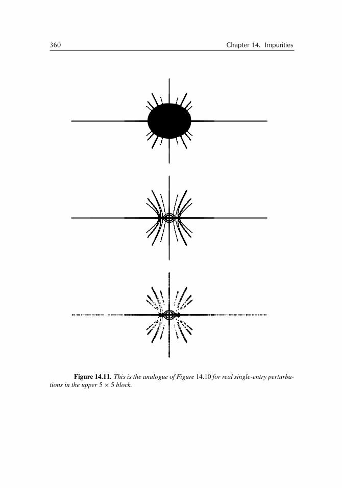
buch72005/10/5page 360

�

�

�

�

�

�

�

�


Figure 14.11. This is the analogue of Figure 14.10 for real single-entry perturba-tions in the upper 5× 5 block.

buch72005/10/5page 361

�

�

�

�

�

�

�

�


−1.5 −1 −0.5 0 0.5 1 1.5

−1

−0.5

0

0.5

1

−1.5 −1 −0.5 0 0.5 1 1.5

−1

−0.5

0

0.5

1

Figure 14.12. Real single-entry perturbations to T (b) and Tn(b) for b(t) = t +19 t−1 and � = [−5, 5]. The top picture is the union of sp(j,k)

� T (b) over (j, k) ∈ N×N. Themiddle picture shows computed eigenvalues of 1000 single-entry perturbations to T50(b),where the perturbed entry is chosen by random anywhere in the matrix, and the perturbationitself is randomly chosen from the uniform distribution on [−5, 5]. The two bottom picturesintend to motivate the dark interior elliptic region in the middle picture. They are explainedin the text.

buch72005/10/5page 362

�

�

�

�

�

�

�

�


(finite volume case) by the union of sp (T50(a)+ ωEjk) for 1000 random choices of j, k ∈{1, 2, . . . , 50} and ω ∈ [−5, 5]. The eigenvalues of the finite Toeplitz matrices Tn(a) arehighly sensitive to perturbations even for modest dimensions. It is interesting that the singleentry perturbations investigated here do not generally change the qualitative nature of thateigenvalue instability. This is revealed for a specific example by the pseudospectral plots atthe bottom of Figure 14.12 (computed using [300]). The interior elliptical region of higheigenvalue concentration in the middle picture is an artifact of finite precision arithmetic;this is revealed by the two bottom pictures, which show the boundaries of the pseudospectraspεT50(b) (left) and spε(T50(b)+ωE54) with ω = −3 (right) for ε = 10−1, 10−3, . . . , 10−15.Dots (·) denote computed eigenvalues; circles (◦) show the true eigenvalue locations. Thisexplains the dark interior ellipse in the center plot of Figure 14.12: Many of these computedeigenvalues are inaccurate due to rounding errors. Generic perturbations of norm 10−15

obscure the effects of our larger, single-entry perturbations. The true structure is moredelicate, as emphasized by Figure 14.13, which zooms in on the middle image of Figure14.11 for perturbations to the upper left 5 × 5 corner of Tn(b). We compare the n → ∞structure to the eigenvalues of perturbations of T10(b) and T50(b). The convergence to theasymptotic limit is compelling, though from an applications perspective, any point in theinterior of b(T) will behave like an eigenvalue when n is large.

Finally, Figure 14.14 exhibits a Toeplitz matrix with six diagonals. The symbol b isgiven by

b(t) = (1.5− 1.2 i)t−1 + (0.34+ 0.84 i)t

+ (−0.46− 0.1 i)t2 + (0.17− 1.17 i)t3 + (−1+ 0.77 i)t4.

Notice again the emergence of many wings, which make the set �(b) (middle picture)become something reminiscent of a horse in cave paintings.

14.5 Can Structured Pseudospectra Jump?Let H be a Hilbert space and let A, B, C ∈ B(H). In accordance with (7.2), we define thestructured pseudospectrum

spB,Cε A = sp A ∪ {

λ /∈ sp A : ‖C(A− λI)−1B‖ ≥ 1/ε}. (14.28)

This section addresses the question whether spB,Cε A can jump as ε ∈ (0,∞) changes

continuously. By virtue of (14.28), this question is equivalent to asking whether the norm‖C(A− λI)−1B‖ may be locally constant. If H = �2(N), we have

sp(j,k)

εDA = sp

Ej ,Ek

ε A,

where Ej is the projection on the j th coordinate. Thus, the question whether

|djk(λ)| = |[T −1(b� − λ)]jk| = ‖EjT−1(b� − λ)Ek‖

can locally be a nonzero constant, which is of importance in connection with Theorem 14.19,amounts to the problem whether sp

Ej ,Ek

ε T (b�) can jump.

buch72005/10/5page 363

�

�

�

�

�

�

�

�

14.5. Can Structured Pseudospectra Jump? 363

n→∞

n = 50

n = 10

Figure 14.13. Closer inspection of Figure 14.11. The top plot shows a portionof limn→∞ sp(j,k)

� Tn(b) over all (j, k) in the top 5 × 5 corner for � = [−5, 5]. Themiddle image shows eigenvalues of 10000 random perturbations to a single entry in the topcorner of T50(b); the bottom image shows the same for T10(b). (The accurate eigenvaluesfor N = 50 were obtained by reducing the nonnormality in the problem via a similaritytransformation.)

Proposition 14.21. Let A, B, C be bounded linear operators on a Hilbert space H andsuppose B or C is compact. Let G∞ denote the unbounded component of C \ sp A and letG be any component of C\sp A. Suppose further that there exists a path � in the plane thatconnects G and G∞ such that C(A−λI)−1B can be analytically continued from G along �

to some function f (λ) defined in some open subset V of G∞ and that f (λ) = C(A−λI)−1B

for λ ∈ V . Then ‖C(A − λI)−1B‖ is either nowhere locally constant in G or identicallyzero in G.

buch72005/10/5page 364

�

�

�

�

�

�

�

�


Figure 14.14. Real single-entry perturbations to Tn(b). The range b(T) of theLaurent polynomial b is seen in the top picture. The middle picture shows sp T50(b) andprovides a very good idea of �(b). The bottom picture depicts the superimposed eigenvaluesof 1000 perturbations of T50(b) in a randomly chosen entry from (1, 1), (2, 2), (3, 3) by arandom number uniformly distributed in [−5, 5].

Of course, here “nowhere locally constant in G” means that there is no open subset ofG on which the function is constant. Proposition 14.21 implies in particular that, providedB or C is compact, spB,C

ε A cannot jump if C \ sp A is connected (which is certainly true forfinite matrices A as well as for selfadjoint or compact operators A).

buch72005/10/5page 365

�

�

�

�

�

�

�

�


Proof. Abbreviate C(A − λI)−1B to f (λ). Pick λ0 ∈ G. Since f (λ0) is compact, thereexist x0, y0 ∈ H of norm 1 such that (x0, f (λ0)y0) = ‖f (λ0)‖. Put h(λ) = (x0, f (λ)y0).The function h is analytic and hence either an open map or constant. In the former case,every neighborhood of λ0 contains a λ1 ∈ G such that

‖f (λ0)‖ = |h(λ0)| < |h(λ1)| = |(x0, f (λ1)y0)| ≤ ‖f (λ1)‖,which shows that ‖f (λ)‖ cannot be locally constant in G. In the latter case, analyticcontinuation of h along � to G∞ and subsequently to infinity yields that the constant valueassumed by h must be zero.

Example 14.22. Let U be the forward shift on �2(Z), that is, (Ux)n = xn−1. Equivalently,U is the Laurent operator L(b) induced by b(t) = t . Then sp U is the unit circle T and thecentral 4× 4 block of the resolvent operator (U − λI)−1 is⎛⎜⎜⎜⎝

0 1 λ λ2

0 0 1 λ

0 0 0 1

0 0 0 0

⎞⎟⎟⎟⎠ and

⎛⎜⎜⎜⎝−1/λ 0 0 0

−1/λ2 −1/λ 0 0

−1/λ3 −1/λ2 −1/λ 0

−1/λ4 −1/λ3 −1/λ2 −1/λ

⎞⎟⎟⎟⎠for |λ| < 1 and |λ| > 1, respectively. Thus, ‖P2(U − λI)−1P2‖ = 1 for |λ| < 1. Inthis case the crucial hypothesis of Proposition 14.21 is not satisfied: although each entryof (U − λI)−1 can be analytically continued from |λ| < 1 to all of C, the result of thiscontinuation is different from the corresponding entry of (U − λI)−1 for |λ| > 1.

Using (14.28) and the explicit expressions for (U−λI)−1 displayed above, it is easy to

compute spP2,P2ε U . Put ε0 =

√2/(3+√5) = 0.618 . . . . There is a continuous and strictly

monotonically increasing function h : [ε0,∞)→ [0,∞) such that h(ε0) = 0, h(∞) = ∞,and

spP2,P2ε U =

⎧⎨⎩{λ ∈ C : |λ| = 1} for 0 < ε ≤ ε0,

{λ ∈ C : 1 ≤ |λ| < 1+ h(ε)} for ε0 < ε ≤ 1,

{λ ∈ C : 0 ≤ |λ| < 1+ h(ε)} for 1 < ε.

Clearly, spP2,P2ε U jumps at ε = 1.

Now let b be a Laurent polynomial of the form

b(t) =s∑

k=−r

bktk, r ≥ 0, s ≥ 0, b−r �= 0, bs �= 0. (14.29)

Conjecture 14.23. Let the Laurent polynomial b be of the form (14.29) and suppose thatone of the operators B and C is compact. If G is any connected component of C \ sp T (b),then ‖CT −1(b − λ)B‖ is either nowhere locally constant in G or identically zero in G.

The rest of this section is devoted to the proof of the following result.

buch72005/10/5page 366

�

�

�

�

�

�

�

�


Theorem 14.24. Suppose B and C are of the form B = Pm1B and C = CPm2 with boundedoperators B and C. Then Conjecture 14.23 is true in each of the following cases:

(a) C \�(b) is connected;

(b) m1 = m2 = 1;

(c) T (b) is Hessenberg, that is, r or s equals 1;

(d) r + s is a prime number and r or s equals 2;

(e) r + s ≤ 5 or r + s = 7.

Before proceeding to the proof, we cite a corollary of Theorem 14.24.

Corollary 14.25. Let b be of the form (14.29) and let G be a connected component ofC\�(b). The function d11 is always nowhere locally constant in G. If j ≥ 1 or k ≥ 1, thenthe function djk is either identically zero in G or nowhere locally constant in G providedone of the following conditions is satisfied:

(a) C \�(b) is connected;

(b) T (b) is Hessenberg, that is, r or s equals 1;

(c) r + s is a prime number and r or s equals 2;

(d) r + s ≤ 5 or r + s = 7.

Proof. Pick λ0 ∈ G. There is a � > 0 such that λ0 ∈ C \ sp T (b�) and djk(λ) =EjT

−1(b� − λ)Ek for all λ in some open neighborhood of λ0. It remains to use Theorem14.24 with b replaced by b�, with m1 = j and B = Ej , and with m2 = k and C = Ek .

We emphasize that C \ �(b) is connected in many cases. This set is in particularconnected if T (b) has at most three nonzero diagonals (see Example 11.18) or if T (b) istriangular (in which case �(b) is a singleton) or if T (b) is Hermitian (which implies that�(b) is a line segment of the real line). We do not know any b with r + s ≤ 5 for whichC \�(b) is disconnected. Theorem 11.20 delivers a b with r = s = 3 such that C \�(b)

is disconnected.

We now turn to the proof of Theorem 14.24. Let b be of the form (14.29) and put

n = r + s, Qn(z) = b−r + b−r+1 + · · · + bszr+s . (14.30)

For λ ∈ C, let z1(λ), . . . , zn(λ) be the zeros of the polynomial Qn(z)− λzr ,

Qn(z)− λzr = bs(z− z1(λ)) · · · (z− zn(λ)). (14.31)

The operator T (b−λ) is invertible if and only if r of the zeros z1(λ), . . . , zn(λ) have modulusless than 1 and the remaining s zeros are of modulus greater than 1. We denote the formerzeros by δ1(λ), . . . , δr (λ) and the latter zeros by μ1(λ), . . . , μs(λ). We put

buch72005/10/5page 367

�

�

�

�

�

�

�

�


μ(λ) = μ1(λ) · · ·μs(λ), u0(λ) = 1, v0(λ) = 1,

um(λ) =∑

α1+···+αs=mαj≥0

μ1(λ)−α1 · · ·μs(λ)−αs (m ≥ 1),

vm(λ) =∑

β1+···+βr=mβj≥0

δ1(λ)β1 · · · δr(λ)βr (m ≥ 1),

U(λ) =

⎛⎜⎜⎝u0(λ)

u1(λ) u0(λ)

u2(λ) u1(λ) u0(λ)

. . . . . . . . . . . .

⎞⎟⎟⎠ ,

V (λ) =

⎛⎜⎜⎝v0(λ) v1(λ) v2(λ) . . .

v0(λ) v1(λ) . . .

v0(λ) . . .

. . .

⎞⎟⎟⎠ .

Then

T −1(b − λ) = (−1)s

bs

· 1

μ(λ)U(λ)V (λ). (14.32)

From (14.32) we see that each entry of T −1(b − λ) is of the form

[T −1(b − λ)]jk = Rjk(δ1(λ), . . . , δr (λ);μ1(λ), . . . , μs(λ)), (14.33)

where Rjk is a rational function of n = r + s variables with coefficients in Z. Moreover,Rjk is symmetric in the first r variables and in the last s variables.

Throughout what follows we let f (λ) = CT −1(b − λ)B and we assume that G issome bounded component of C \ sp T (b).

We consider the Riemann surface of Qn(z) − λzr = 0. The points λ ∈ C for whichQn(z) − λzr has a multiple zero are called the finite branch points. There exist at most n

finite branch points. We denote them by λ1, . . . , λk . The point at infinity is also a branchpoint. Thus, the set of all branch points is

W := {λ1, . . . , λk,∞}.We join λ1 to λ2 by a cut S1, λ2 to λ3 by a cut S2, . . . , and λk to∞ by a cut Sk . Put

S = S1 ∪ · · · ∪ Sk ∪W.

We can draw S1, . . . , Sk so that C \ S is connected. The zeros in (14.31) can be chosen sothat z1(λ), . . . , zn(λ) are analytic functions in C\S. Take n copies �1, . . . , �n of C\S andthink of zj as a map of �j to C. We glue �i and �j along the cut S� whenever the functionzi(λ) can be continued analytically to the function zj (λ) across S�. The resulting set � isthe Riemann surface of Qn(z)− λzr = 0, and �j is referred to as the j th branch of �.

Each path in C \W induces a permutation of the branches of � in a natural way. Theset of all these permutations is a group G, the monodromy group of Qn(z)−λzr = 0. Let πj

buch72005/10/5page 368

�

�

�

�

�

�

�

�


(j = 1, . . . , k) be the permutation corresponding to a small counterclockwise-oriented circlearound the branch point λj . Clearly, G contains π1, . . . , πk . We put π∞ = π1 . . . πk . Thus,π∞ is the permutation of the branches resulting from a large counterclockwise-oriented circlecontaining all finite branch points in its interior. The group G is generated by π1, . . . , πk .

Let λ ∈ C \ sp T (b). We have |zj (λ)| < 1 for exactly r values of j . We call thebranches �j corresponding to these values of j the small branches at λ. The s branches �j

for which |zj (λ)| > 1 will be called the large branches at λ.

Proposition 14.26. If there is a π ∈ G that permutes the set of the small branches at thepoints of G to the set of the small branches at the points of the unbounded component G∞,then ‖f (λ)‖ is either nowhere locally constant in G or identically zero in G.

Proof. Let � be the path in C \W that corresponds to the permutation π . From (14.32) and(14.33) we see that each entry of Pm2T

−1(b−λ)Pm1 and hence also CPm2T−1(b−λ)Pm1B

can be analytically continued along �. Since π permutes the small branches into themselves,the result of the analytic continuation coincides with the operator CPm2T

−1(b − λ)Pm1B

for λ ∈ G∞. It remains to apply Proposition 14.21.

From Chapter 11 we know that when labelling the zeros z1(λ), . . . , zr+s(λ) of (14.31)so that

|z1(λ)| ≤ |z2(λ)| ≤ · · · ≤ |zr+s(λ)|, (14.34)

then

�(b) = {λ ∈ C : |zr(λ)| = |zr+1(λ)|}. (14.35)

Proof of Theorem 14.24(a). Pick a point λ0 ∈ G. Since C \�(b) is connected, there is apath � in C \ (W ∪ �(b)) joining λ0 to infinity. By (14.35), we have |zr(λ)| < |zr+1(λ)|throughout this path. This means that when moving along this path we will eventually stayin the r small branches of � at infinity. In other words, there is a π ∈ G permuting theset of the small branches at λ0 to the set of the small branches at infinity. The assertion istherefore immediate from Proposition 14.26.

The group G is said to be r-transitive if for every two r-tuples (�i1 , . . . , �ir ) and(�j1 , . . . , �jr

) of r distinct branches of � there is a π ∈ G such that

π(�i1) = �j1 , . . . , π(�ir ) = �jr.

We call the group G weakly r-transitive if for every two sets {�i1 , . . . , �ir } and {�j1 , . . . , �jr}

of r distinct branches of � there exists a π ∈ G such that

{π(�i1), . . . , π(�ir )} = {�j1 , . . . , �jr},

i.e., such that π(�i1), . . . , π(�ir ) coincide with �j1 , . . . , �jrup to the arrangement. Clearly,

weak 1-transitivity and 1-transitivity are equivalent.

Proposition 14.27. If the monodromy group of Qn(z) − λzr = 0 is weakly r-transitive,then ‖f (λ)‖ is either nowhere locally constant in G or identically zero in G.

buch72005/10/5page 369

�

�

�

�

�

�

�

�


Proof. Weak r-transitivity means that we can permute any prescribed set of r branches intoany prescribed set of r branches. We can in particular permute the r small branches at thepoints of G into the r small branches at the points of G∞. The assertion is therefore a directconsequence of Proposition 14.26.

Proposition 14.28. The monodromy group of the polynomial Qn(z) − λzr = 0 is always1-transitive.

Proof. It is well known (see, e.g., [175, Section 4.14]) that G is 1-transitive if and only ifQn(z)− λzr is irreducible in C[z, λ]. But the irreducibility of Qn(z)− λzr in C[z, λ] canbe readily verified.

Proof of Theorem 14.24(b). Let λ be a point in C \ sp T (b). We label the zeros z1(λ), . . . ,

zr+s(λ) so that (14.34) holds. Thus, the small branches at λ are �1, . . . , �r and the largebranches at λ are �r+1, . . . , �r+s . By formula (14.32), the function g(λ) := [T −1(b−λ)]11

equals

(−1)sb−1s μ1(λ)−1 · · ·μs(λ)−1 = (−1)sb−1

s zr+1(λ)−1 · · · zr+s(λ)−1.

This shows that g(λ) �= 0. Since the group G is 1-transitive (Proposition 14.28), there is apath in C\W starting and terminating at λ such that the s large branches at λ are permuted intos branches �i1 , . . . , �is containing at least one small branch. Consequently, after analyticcontinuation along this curve, g(λ) becomes zi1(λ)−1 . . . zis (λ)−1, and because, obviously,

|zi1(λ) · · · zis (λ)| < |zr+1(λ) · · · zr+s(λ)|,it follows that |g(λ)| cannot be locally constant. Since f (λ) = CP1g(λ)P1B = g(λ)CP1B,we arrive at the conclusion that ‖f (λ)‖ = |g(λ)| ‖CP1B‖ is either identically zero ornowhere locally constant in �.

Proof of Theorem 14.24(c). Without loss of generality assume r = 1; the case s = 1 can bereduced to the case r = 1 by passage to adjoint operators. Combining Propositions 14.27and 14.28 we arrive at the assertion.

We now turn to the case n = r + s = 4. By what was already proved, we are leftwith the constellation r = s = 2. Everything would be fine if the monodromy group ofQ4(z)− λz2 = 0 were always weakly 2-transitive (Proposition 14.27). Unfortunately, thisneed not be the case. Indeed, let Q4(z)be the polynomial μz2 + (z − α)2(z − β)2, whereα, β, μ ∈ C, α �= β, and αβ �= 0. We have exactly two finite branch points, λ1 (= μ) andλ2, and the monodromy group is generated by π1 = (12)(43) and π2 = (13)(24). Hereand in what follows we identify �1, �2, . . . with the numbers 1, 2, . . . . Clearly, we cannotpermute {1, 2} into {1, 3}. Fortunately, in this case we can have recourse to Theorem 11.20,which shows that C \�(b) is connected.

Let us return for a moment to the case of general n and r, s. The permutation π

associated with a branch point λ can be written as a product of cycles. We say that λ is ofthe type (L1, L2, . . . ) if the cycle lengths of π are L1, L2, . . . . In the previous paragraph,we encountered two finite branch points of the type (2, 2).

Proposition 14.29. If all finite branch points of the Riemann surface of the polynomial

buch72005/10/5page 370

�

�

�

�

�

�

�

�


Qn(z)−λz2 = 0 are of the type (2, 1, . . . , 1), then the monodromy group of Qn(z)−λz2 = 0is weakly 2-transitive.

Proof. It suffices to show that we can permute {1, 2} to {1, m} for arbitrary m �= 1. Letλ1, . . . , λk be the finite branch points. Without loss of generality suppose that the permuta-tions (12), (13), . . . , (1 p) are among π1, . . . , πk and that the permutations (1 p + 1), . . . ,

(1n) are not among π1, . . . , πk . It is easily seen that we can permute {1, 2} to {1, m} forevery m ∈ {2, . . . , r}. Thus, let m ≥ p + 1. Since G is 1-transitive (Proposition 14.28),there is a path on � joining �1 to �m. This path goes through the branches x1, x2, . . . , x�

and we may assume that xj �= 1 and xj �= m for all j and that x1 ∈ {2, . . . , p}. As eachbranch point is of the type (2, 1, . . . , 1), it follows that the path goes from the branch x1 tothe branch 1 and stays there. Thus, we can permute {1, x1} to {1, m}.

Proposition 14.30. If r = s = 2, then ‖f (λ)‖ is either nowhere locally constant in G oridentically zero in G.

Proof. If there is a λ such that Q4(z)− λz2 has two distinct zeros of multiplicity 2 or onezero of multiplicity 4, then the polynomial Q4(z) is of the form

λz2 + (z− α)2(z− β)2,

and the assertion follows from Theorem 11.20 and Theorem 14.24(a). Thus, we may restrictourselves to the case where all of the (at most four) finite branch points are of the types (3, 1)

or (2, 1, 1). It is easily seen that the branch point at infinity is of the type (2, 2). Our goal isto show that G is weakly 2-transitive so that the present theorem follows from Proposition14.27.

If all finite branch points have the type (2, 1, 1), then Proposition 14.29 implies weak2-transitivity. Thus, assume there is at least one finite branch point, λ1, of the type (3, 1)

and that π1 = (123). Since G is 1-transitive, there must exist at least one more finite branchpoint λ2.

We first consider the case where all finite branch points different from λ1 are of thetype (2, 1, 1). As G is 1-transitive, branch 4 must be in the cycle of length 2 of one of thesebranch points, say λ2. By symmetry, we may assume that the permutation π2 is (14). Buta group of permutations of 1, 2, 3, 4 containing π1 = (123) and π2 = (14) is easily seen tobe weakly 2-transitive.

We are left with the case where λ2 is of the type (3, 1). If branch 4 is in the cycle oflength 3 of π2, then G is readily checked to be weakly 2-transitive. So assume branch 4 isleft fixed by π2. Then there must exist a third finite branch point λ3 of the type (2, 1, 1) suchthat branch 4 is contained in a cycle of length 2. By direct inspection of the few possiblecases one sees that the group G is always weakly 2-transitive.

Lemma 14.31. The order of the monodromy group G of Qn(z)− λzr = 0 is divisible by n.

Proof. For 1 ≤ j ≤ n, let Gj = {π ∈ G : π(1) = j}. Clearly, G = G1 ∪ · · · ∪ Gn andGi ∩Gj = ∅ for i �= j . Given two distinct numbers i, j in {1, . . . , n}, we can find a σ ∈ Gsuch that σ(i) = j (Proposition 14.28). The map Gi → Gj , π �→ σπ is obviously bijective.

buch72005/10/5page 371

�

�

�

�

�

�

�

�


This implies that all the sets Gj have the same number of elements, say �. Consequently,the order of G is n�.

Lemma 14.32. If n is a prime number, then the monodromy group G of the polynomialQn(z) − λzr = 0 contains an n-cycle, that is, after appropriately labelling the branches,(12 . . . n) ∈ G.

Proof. This follows from Lemma 14.31 and a well-known theorem by Cauchy, which saysthat if n is a prime and the order of a finite group is divisible by n, then the group containsan element of the order n.

Lemma 14.33 (well known). If a subgroup G of the full symmetric group Sn contains ann-cycle and a transposition, then G = Sn.

Proof of Theorem 14.24(d). If r = 2 or s = 2, then the branch point at infinity of theRiemann surface of Qn(z)−λzr = 0 is of the type (n−2, 2). Hence πn−2∞ is a transposition(notice that n− 2 is odd). Combining Proposition 14.27 with Lemmas 14.32 and 14.33, wearrive at the assertion.

Proof of Theorem 14.24(e). Without loss of generality, assume r ≤ s. Parts (a) and (c) ofTheorem 14.24 imply the desired result for r = 0 and r = 1. Proposition 14.30 disposes ofthe case r = s = 2, and Theorem 14.24(d) gives the assertion for r = 2, s = 3 and r = 2,s = 5. We are left with the case where r = 3 and s = 4. In this case we deduce from Lemma14.32 that G contains a 7-cycle, say π = (12 . . . 7). The branch point at infinity providesus with a permutation of the type σ = (1xyz)(abc). By checking all possible cases, onesees that the group generated by π and σ is always weakly 3-transitive. It remains to makeuse of Proposition 14.27.

Remark. The arguments used above are standard in Galois theory, and in fact the mon-odromy group G of Qn(z)− λzr = 0 is known to be isomorphic to the Galois group G0 ofQn(z)− λzr = 0. Let R = C(λ) be the field of the rational functions (of λ) with complexcoefficients. We think of Qn(z)−λzr as an element of R[z]. The splitting field of this poly-nomial is R(z1(λ), . . . , zn(λ)), where z1(λ), . . . , zn(λ) are given by (14.31). The Galoisgroup G0 may be identified with the group of all permutations of z1(λ), . . . , zn(λ) that canbe extended to an automorphism of the field R(z1(λ), . . . , zn(λ)) that leaves the elements ofR fixed. When working with the monodromy group, we transform valid equalities into newequalities by analytic continuation, while from the algebraic point of view, valid equalitiesare transformed into new equalities by the action of the Galois group.

The polynomial Qn(z)− λzr can be shown to be the minimal polynomial of each ofits zeros z1(λ), . . . , zn(λ). This implies that the dimension of R(z1(λ)) overR is n. Lemma14.31 so amounts to saying that this dimension divides the order of G0, and this is one ofthe conclusions of the fundamental theorem of Galois theory.

buch72005/10/5page 372

�

�

�

�

�

�

�

�


Exercises

1. Let Un(λ) denote the Chebyshev polynomial of the second kind introduced in Section1.9.

(a) Show that the eigenvalues of Tn(σ ) + vEnn are the zeros of the polynomialUn(λ/2)− vUn−1(λ/2).

(b) Let λj be an eigenvalue of Tn(σ )+ vEnn and let θj ∈ C be any number such thatcos θj = λj . Prove that

xj =(

2 sin(kθj )√2n+ 1− U2n(λj/2)

)n

k=1

is an eigenvector for λj and that ‖xj‖2 = 1.

(c) Use (b) to show that the eigenvector xj is extended for |λj | ≤ 2 and localized for|λj | > 2.

2. Let An = Tn(σ )+ vIn,n, where v is uniformly distributed in [−M, M] and In,n is then× n identity matrix. The density of the eigenvalues of An is defined as

�n(λ) = E

⎛⎝1

n

n∑j=1

δ(λ− λj (An))

⎞⎠ .

By Theorem 2.4,

�n(λ) = 1

2Mn

∫ M

−M

n∑j=1

δ

(λ− v − 2 cos

πj

n+ 1

)dv.

Clearly, �n(λ) = 0 for λ ∈ C \ R. Prove that for λ ∈ R,

limn→∞ �n(λ) = 1

2Mπ

∫ λ+M

λ−M

χ[−2,2](x)√4− x2

dx,

where χ[−2,2](x) is 1 for −2 ≤ x ≤ 2 and zero otherwise.

3. (a) Let a ∈ W and λ ∈ C \ sp T (a). Show that

[T −1(a − λ)]1,1 = 1/G(a − λ),

where G(b) is defined by (2.25), and deduce that

sp(1,1)

εDT (a) = sp T (a) ∪ {λ /∈ sp T (a) : G(|a − λ|) ≤ ε}.

(b) Show that there is a dense subset M of W such that if a ∈M, then sp(1,1)

εDT (a) is

strictly larger than sp T (a) for every ε > 0.

buch72005/10/5page 373

�

�

�

�

�

�

�

�

Exercises 373

4. For a ∈ W , we denote by L(a) the Laurent matrix (aj−k)∞j,k=−∞ (recall the notes to

Chapter 1).

(a) Show that L(a) generates a bounded operator on �2(Z).

(b) Show that sp L(a) = a(T).

(c) Prove that spm

εDL(a) = sp L(a) for all sufficiently small ε > 0 if and only if

max|k|≤m−1sup

λ/∈a(T)

∣∣∣∣∫ 2π

0

eikθ

a(eiθ )− λdθ

∣∣∣∣ <∞.

(d) Deduce that if a ∈ P is real valued on T, then spm

εDL(a) is strictly larger than

sp L(a) for every ε > 0.

5. Show that the matrix ⎛⎜⎜⎜⎜⎝v1 eg1 e−gn

e−g1 v2 eg2

. . . . . . . . .

e−gn−2 vn−1 egn−1

egn e−gn−1 vn

⎞⎟⎟⎟⎟⎠is similar to the matrix ⎛⎜⎜⎜⎜⎝

v1 eg e−g

e−g v2 eg

. . . . . . . . .

e−g vn−1 eg

eg e−g vn

⎞⎟⎟⎟⎟⎠ ,

where g = (g1 + · · · + gn)/n.

6. Show that the matrix⎛⎜⎜⎜⎜⎝v1 α2

1 v2 α2

. . . . . . . . .

1 vn−1 α2

1 vn

⎞⎟⎟⎟⎟⎠ (α �= 0)

is similar to the matrix

α

⎛⎜⎜⎜⎜⎝v1/α 1

1 v2/α 1. . . . . . . . .

1 vn−1/α 11 vn/α

⎞⎟⎟⎟⎟⎠ .

buch72005/10/5page 374

�

�

�

�

�

�

�

�


7. Show that the matrix ⎛⎜⎜⎜⎜⎜⎝v1 1

v2 1. . .

. . .

vn−1 1vn

⎞⎟⎟⎟⎟⎟⎠is similar to the matrix ⎛⎜⎜⎜⎜⎜⎝

v1 β

v2 β

. . .. . .

vn−1 β

β−n vn

⎞⎟⎟⎟⎟⎟⎠ .

8. Show that ⎛⎝ a −1b −1

c

⎞⎠−1

=⎛⎝ a−1 a−1b−1 a−1b−1c−1

b−1 b−1c−1

c−1

⎞⎠and generalize the result from 3× 3 to n× n matrices.

9. Let A be an n× n matrix and let u and v be column vectors of length n. Show that

det (A+ uv�) = det A+ v� adj (A) u,

where adj (A) is the adjugate matrix of A.

Notes

The study of discrete Hamiltonians, either with deterministic or with random potential Vn,is a big business and goes beyond the scope of the present book. We therefore leave thingswith a few remarks.

Anderson [4] considered the selfadjoint matrix Tn(σ ) with random perturbations onthe main diagonal and discovered numerically that the eigenvectors for eigenvalues outsidethe original spectrum in [−2, 2] are localized. Figure 14.15 illustrates the phenomenon.The top picture shows the 50 eigenvalues of the matrix T50(σ ) + diag (vj )

50j=1 for a single

realization of 50 independent vj ’s drawn from the uniform distribution on [−1, 1]. The(extended) eigenvector for the encircled eigenvalue in the middle is shown in the bottomleft picture, and the (localized) eigenvector for the encircled boundary eigenvalue is seen inthe bottom right picture.

The discrete Laplacian Tn(σ ) is selfadjoint, as it should be in quantum mechanics. Theinterest in randomly perturbed general tridiagonal Toeplitz matrices Tn(t + α2t−1) comesfrom so-called non-Hermitian quantum mechanics and was pioneered by Hatano and Nelson

buch72005/10/5page 375

�

�

�

�

�

�

�

�

Notes 375

−2 −1 0 1 2−1

−0.8

−0.6

−0.4

−0.2

0

0.2

0.4

0.6

0.8

1

0 20 40

−0.5

−0.4

−0.3

−0.2

−0.1

0

0.1

0.2

0.3

0.4

0.5

0 20 40

−0.5

−0.4

−0.3

−0.2

−0.1

0

0.1

0.2

0.3

0.4

0.5

Figure 14.15. The Anderson model.

[152]. Their discovery is illustrated in Figure 14.16. To make the effect more visible, onereplaces Tn(t+α2t−1) by Cn(t+α2t−1). In the top picture we plotted the 50 eigenvalues ofCn(t + 0.49t−1)+ diag (vj )

50j=1 for a single realization of 50 independent diagonal entries

vj from the uniform distribution on [−1, 1]. We see a bubble and two wings. The absolutevalue of the (extended) eigenvector for the encircled eigenvalue on the bubble is shown inthe bottom left picture; the absolute value of the (localized) eigenvector for the encircledeigenvector on the wing is in the bottom right picture.

Profound theoretical investigations about this topic are due to Brézin and Zee [75],Brouwer, Silvestrov, and Beenakker [76], Davies [95], Feinberg and Zee [117], [118],Goldsheid and Khoruzhenko [135], [136], and Janik et al. [173], to cite only a few figures.Applications to population dynamics appear in [91], [191], and applications to small worldnetworks can be found in [189], [259], for instance. An introduction to the ideas of Feinbergand Zee follows below.

In this chapter we confine ourselves to showing how structured pseudospectra canbe employed in order to get interesting information about the possible spectra of banded(and not necessarily Hermitian) Toeplitz matrices with impurities. The idea of formulating

buch72005/10/5page 376

�

�

�

�

�

�

�

�


−2 −1 0 1 2−1

−0.8

−0.6

−0.4

−0.2

0

0.2

0.4

0.6

0.8

1

0 20 40−0.1

0

0.1

0.2

0.3

0.4

0.5

0 20 40−0.1

0

0.1

0.2

0.3

0.4

0.5

Figure 14.16. The Hatano-Nelson model.

problems on random Toeplitz matrices in the language of pseudospectral analysis goes backto Trefethen, Contedini, and Embree [274]. For the reader’s convenience, we cite their mainresults below. The approach of [274] depends heavily on the circumstance that a simpleexplicit inverse for bidiagonal matrices is available (see Exercise 8). For matrices withmore than two diagonals, things become significantly more intricate. Papers [41] to [44] aredevoted to this more general situation and exhibit several phenomena that can be explainedwith the help and in the language of structured pseudospectra.

The purpose of Section 14.1 is to illustrate a few phenomena by a transparent example.Paper [189] is closely related to this section. The results of Section 14.2 were establishedin [43], and Section 14.3 is based on [42]. In Section 14.4 we follow [44]. All of Section14.5 is from [50].

Exercise 3 is a result of [122]. Exercises 3 and 4 are from [42]. These two exercisesreveal that Theorem 14.8 is not a consequence of some sort of general perturbation theory.Exercise 5 is taken from [91]. Exercise 7 is probably well known. We found it in [274].Note that if |β| is large, then the matrix with the β’s differs from a purely bidiagonal matrixin an exponentially small term only—the spectral properties of Cn(χ) + random diagonal

buch72005/10/5page 377

�

�

�

�

�

�

�

�

Notes 377

and Tn(χ1) + random diagonal are nevertheless significantly different. Exercise 8 is thebasis of the approach of [274], because it delivers explicit expressions for the entries of theinverse of the matrix λI − (Tn(χ1)+ diag (vj )). Exercise 9 is explicit in [233].

Further results: Arveson and C∗-algebras II. The following is intended as anotherillustration of the usefulness of C∗-algebras in numerical analysis on the one hand and asanother instance of the emergence of Toeplitz plus diagonal matrices on the other. Theresults and ideas cited here are due to Arveson [7], [8], [9] (see also [21], [22], [149]).

The general problem is to find the spectrum of a selfadjoint operator A in B(�2(Z))

by spectral approximation, say by considering the 2n× 2n matrices

An = PnAPn|Im Pn,

where now (in contrast to the rest of the book) Pn denotes the projection on �2(Z) definedby

Pn : {ξk}∞k=−∞ �→ {. . . , 0, ξ−n, . . . , ξ−1, ξ0, . . . , ξn−1, 0, . . . }.Put Qn = I − Pn. The Følner algebra F({Pn}) associated with the sequence {Pn}∞n=1 is theC∗-subalgebra of B(�2(Z)) that is constituted by all operators A for which

limn→∞

tr PnA∗QnAPn

n= 0, lim

n→∞tr PnAQnA

∗Pn

n= 0.

It is easily seen that F({Pn}) contains all bounded Laurent operators and all bounded diag-onal operators.

A tracial state of a unital C∗-algebra A is a bounded linear functional τ : A → Csatisfying τ(a∗a) ≥ 0 and τ(ab) = τ(ba) for all a, b ∈ A and τ(e) = 1 for the unit e ofA. A unital C∗-algebra is said to have a unique tracial state if the set of its tracial states isa singleton.

Let A have a unique tracial state τ . Then for each selfadjoint a ∈ A the mapC0(R) → C, ϕ �→ τ(ϕ(a)) is a positive linear functional. (Here C0(R) stands for thecompactly supported continuous functions on R.) By the Riesz-Markov theorem, there is aprobability measure μa on R such that

τ(ϕ(a)) =∫ ∞

−∞ϕ(x)dμa(x) for all ϕ ∈ C0(R).

This measure μa is called the spectral distribution of a.

Arveson’s theorem. Let A be a unital C∗-subalgebra of the Følner algebra F({Pn}) andsuppose A has a unique tracial state τ . Let A ∈ A be a selfadjoint operator, let λj (An)

(j = 1, . . . , 2n) be the eigenvalues of An, and let μA be the spectral distribution of A. Then

limn→∞

1

2n

2n∑j=1

ϕ(λj (An)) =∫ ∞

−∞ϕ(x)f μA(x) for every ϕ ∈ C0(R). (14.36)

An irrational rotation C∗-algebra is a C∗-algebra that is generated by two unitaryelements u and v which satisfy uv = e2πiθ vu with some irrational number θ ∈ R. It

buch72005/10/5page 378

�

�

�

�

�

�

�

�


turns out that all such algebras with the same θ are isomorphic. To be more precise, ifA(j) (j = 1, 2) are C∗-algebras that are generated by unitary elements uj , vj satisfyingujvj = e2πiθ vjuj , then the map u1 �→ u2, v1 �→ v2 extends to a C∗-algebra isomorphismof A(1) onto A(2).

A simple example of an irrational rotation C∗-algebra is the C∗-subalgebra ofB(�2(Z))

that is generated by the two unitary operators

(Uξ)n = ξn−1, (V ξ)n = e−2πinθ ξn. (14.37)

We denote this C∗-algebra by Aθ . Since, obviously, U and V belong to the Følner algebraF({Pn}), the entire C∗-algebra Aθ is contained in F({Pn}). One can also show that Aθ hasa unique tracial state.

Let us now turn to quantum mechanics. The one-dimensional Hamiltonian

(Hf )(x) = −1

2f ′′(x)+ ψ(x)f (x)

is discretized by

Hδ = 1

2P 2

δ + ψ(Qδ),

where δ, the numerical step size, is a small positive rational number and Pδ , Qδ (whichshould not be confused with the projections Pn, Qn introduced above) are the selfadjointoperators defined on L2(R) by

(Pδf )(x) = f (x + δ)− f (x − δ)

2iδ, (Qδf )(x) = sin(δx)

δf (x).

With the unitary operators U and V given on L2(R) by

(Uδf )(x) = f (x + 2δ), (Vδf )(x) = eiδxf (x),

we have

Hδ = − 1

8δ2

[Uδ + U ∗

δ − 8δ2 ψ

(1

2iδ(Vδ − V ∗

δ )

)]+ 1

4δ2I. (14.38)

It is easily seen that UδVδ = e2iδ2VδUδ = e2πi(δ2/π)VδUδ . By what was said above, the

C∗-algebra generated by Uδ and Vδ is isomorphic to Aδ2/π (recall that δ is rational and thathence δ2/π is irrational). We may therefore identify the operator in the brackets of (14.38)with the operator

A = U + U ∗ − 8δ2 ψ

(1

2iδ(V − V ∗)

)∈ Aθ ⊂ B(�2(Z)), (14.39)

where U and V are given by (14.37) with θ = δ2/π . Clearly, we can write (14.39) in theform

A = L(χ−1 + χ1)+ diag (vj )∞j=−∞ ∈ Aθ ⊂ B(�2(Z)) (14.40)

buch72005/10/5page 379

�

�

�

�

�

�

�

�

Notes 379

with vj = −8δ2 ψ((−1/δ) sin(2jδ2)). Application of Arveson’s theorem now yields that(14.36) is true with

An =

⎛⎜⎜⎜⎜⎝v−n 11 v−n+1 1

. . . . . . . . .

1 vn−2 11 vn−1

⎞⎟⎟⎟⎟⎠= T2n(χ−1 + χ1)+ diag (vj )

n−1j=−n

and thus sets at least a theoretical foundation for the spectral approximation of A and henceHδ .

Further results: Feinberg and Zee. The following material is taken from [117] and [118].Let An be a random n× n matrix. The eigenvalue density of An is

�(λ) = E

⎛⎝1

n

n∑j=1

δ(λ− λj (An))

⎞⎠ ,

where E denotes the expected value (= mean) and δ is the Dirac delta function. The keyformulas for computing �(λ) are

�(λ) = 1

π∂∗E

(1

ntr [(λI − AnI)−1]

), (14.41)

= 1

π∂ ∂∗E

(1

nlog det (λI − An)(λI − A∗n)

), (14.42)

where

∂∗ = ∂

∂λ= 1

2

(∂

∂x+ i

∂

∂y

), ∂ = ∂

∂λ= 1

2

(∂

∂x− i

∂

∂y

).

The function in the parentheses on the right of (14.41) is called Green’s function and denotedby G(λ). Thus,

�(λ) = 1

π∂∗G(λ), G(λ) = E

(1

ntr [(λI − AnI)−1]

).

Let now An = Tn(b)+vE11 where b ∈ P is fixed and v is drawn from some probabilitydistribution. If |λ| is large, we have

(λI − An)−1 = (Cn(λ− b)− vE11)

−1 = (I − C−1n (λ− b)vE11)

−1C−1n (λ− b)

= C−1n (λ− b)+

∞∑k=1

vk([C−1n (λ− b)]11)

k−1C−1n (λ− b)E11C

−1n (λ− b)

and hence1

ntr [(λI − An)

−1]

= 1

ntr C−1

n (λ− b)+∞∑

k=1

vk([C−1n (λ− b)]11)

k−1tr C−1n (λ− b)E11C

−1n (λ− b).

buch72005/10/5page 380

�

�

�

�

�

�

�

�


We know from Proposition 2.1 that

C−1n (λ− b) = U ∗

n diag1

λ− b(ωjn)

Un, C−2n (λ− b) = U ∗

n diag1

(λ− b(ωjn))2

Un,

where ωn = e2πi/n. Put

G0(λ) = 1

ntr C−1

n (λ− b) = 1

n

n−1∑j=0

1

λ− b(ωjn)

.

Then

tr E11C−2n (λ− b)E11 = [C−2

n (λ− b)]11 = 1

n

n−1∑j=0

1

(λ− b(ωjn))2

= −∂G0(λ)

∂λ

and consequently,

G(λ) = G0(λ)− 1

n

∂G0(λ)

∂λE

(v

1−G0(λ)v

). (14.43)

As both sides of (14.43) are analytic functions of λ, equality (14.43) is actually true for allλ outside sp Cn(b) = {b(1), b(ωn), . . . , b(ωn−1

n )}.Now take b(t) = χ1(t) := t . For large n,

G0(λ) = 1

n

n−1∑j=0

1

λ− ωjn

≈ 1

2π

∫ 2π

0

dθ

λ− eiθ=

{0 for |λ| < 1,

1/λ for |λ| > 1,

and thus, by (14.43),

G(λ) ≈{

0 for |λ| < 1,1λ+ 1

nλE

(v

λ−v

)for |λ| > 1.

With the Heaviside function H(x) = 0 for x < 0 and H(x) = 1 for x > 1, we can write

G(λ) ≈ H(λλ− 1)

[1

λ+ 1

nλE

(v

λ− v

)]. (14.44)

As a first concrete example, assume v takes the two values r and−r with equal probability,

P(v = r) = P(v = −r) = 1

2. (14.45)

Then (14.44) becomes

G(λ) ≈ H(λλ− 1)

[1

λ+ 1

2nλ

(r

λ− r− r

λ+ r

)]= H(λλ− 1)

[(1− 1

n

)1

λ+ 1

2n

(1

λ− r+ 1

λ+ r

)].

buch72005/10/5page 381

�

�

�

�

�

�

�

�

Notes 381

Taking into account that H ′(x) = δ(x) and ∂∗(1/λ) = πδ(λ) we get

π�(λ) = ∂∗G(λ)

≈ δ(λλ− 1)

[1− 1

n+ λ

2n

(r

λ− r+ r

λ+ r

)]+H(λλ− 1)

[(1− 1

n

)πδ(λ)+ 1

2nπδ(λ− r)+ 1

2nπδ(λ+ r)

].

We have δ(λ) = 0 for |λ| > 1, and the term

δ(λλ− 1)λ

2n

(r

λ− r+ r

λ+ r

)can be neglected for large n. In summary

�(λ) ≈ 1

π

(1− 1

n

)δ(|λ|2 − 1)+H(|λ|2 − 1)

[1

2nδ(λ− r)+ 1

2nδ(λ+ r)

].

Thus, in the n → ∞ limit, the situation is as follows. If r ∈ (0, 1), then the eigenvaluesare distributed on T, and if r ∈ (1,∞), then n− 2 eigenvalues are distributed on T, whiletwo eigenvalues are located at−r and r with the density 1/(2n). Notice that the coefficient1/π before δ(|λ|2 − 1) is correct, since if � is any region containing T, then∫

�

1

πδ(|λ|2 − 1) dA(λ) =

∫ 2π

0

∫ 1+ε

1−ε

1

πδ(r2 − 1) rdrdθ

= 2∫ 1+ε

1−ε

δ(r2 − 1) rdr = 2∫ (1+ε)2

(1−ε)2δ(s − 1)

1

2ds = 1.

We remark that the special distribution (14.45) can also be treated in a more elementarymanner. Namely, the eigenvalues of Cn(χ1) + vE11 are the roots of the polynomial λn −vλn−1 − 1. If |v| > 1 then, in the n →∞ limit, one of these roots is at v with the density1/n and the remaining roots are distributed on T. If |v| ≤ 1 then, in the n →∞ limit, allzeros are distributed on T.

We now take v from the uniform distribution on [−M, M]. Proceeding as above, onecan show that then

G(λ) ≈ H(λλ− 1)

[(1− 1

n

)1

λ− 1

2nMlog

λ−M

λ+M

]and

�(λ) ≈ 1

π

(1− 1

n

)δ(|λ|2 − 1)+ H(|λ|2 − 1)

2nMδ(Im λ)H(M − |Re λ|).

We see in particular that if M > 1, then asymptotically the eigenvalues lie on T and twowings [−M,−1] and [1, M]. Figure 14.17 shows the results of two numerical realizations.

If x = (x1, . . . , xn) is an eigenvector for Cn(χ1) + vE11, then xj+1 = λxj forj = 2, . . . , n− 1. Thus, if |λ| = 1 then x is extended, whereas for λ = ±r with r > 1 thevector x is localized at the beginning.

buch72005/10/5page 382

�

�

�

�

�

�

�

�


−2 −1 0 1 2

−2

−1.5

−1

−0.5

0

0.5

1

1.5

2

−2 −1 0 1 2

−2

−1.5

−1

−0.5

0

0.5

1

1.5

2

Figure 14.17. The superposition of the eigenvalues of C100(χ1) + vE11 for 50random choices of v. In the left picture, v takes the values−2 and 2 with equal probability.In the right picture, v is drawn from the uniform distribution on the segment [−2, 2].

Feinberg and Zee also consider An = Cn(χ1) + diag (v1, . . . , vn), where the vj areindependent and P(vj = r) = P(vj = −r) = 1/2 for all j . In this case one can employ(14.42). In the case at hand,

det An =(

n∏k=1

(λ− vj )

)− 1

and hence

E[log det (λI − An)] = 1

2n

n∑j=0

(n

j

)log

[(λ− r)j (λ+ r)n−j − 1

].

In the limit n→∞, the binomial coefficients are sharply peaked around j ≈ n/2, and thus

E[log det (λI − An)] ≈ log[(λ− r)n/2(λ+ r)n/2 − 1

]. (14.46)

A similar approximation is true for E[log det (λI − A∗n)]. By (14.42), the support of thedensity �(λ) is the singularities of the right-hand side of (14.46). These singularities occurat (λ2 − r2)n/2 = 1, that is, at

λj = ±√

r2 + e4πij/n (j = 0, 1, . . . , n/2). (14.47)

It follows that the original circle spectrum is distorted by the specific randomness consideredinto the curve λ2 = r2 + eiθ (0 ≤ θ < 2π ). Figure 14.18 shows some examples.

Further results: Trefethen, Contedini, and Embree. All of the following is from [274].This paper is devoted to matrices of the form Tn(χ1) + random diagonal and to Cn(χ1) +random diagonal, and it exhibits a Hatano-Nelson bubble and an associated localization-delocalization phenomenon in the context of pseudospectra and resolvents instead of eigen-values and eigenvectors.

buch72005/10/5page 383

�

�

�

�

�

�

�

�

Notes 383

−1.5 −1 −0.5 0 0.5 1 1.5

−1.5

−1

−0.5

0

0.5

1

1.5

r = 0.5

−1.5 −1 −0.5 0 0.5 1 1.5

−1.5

−1

−0.5

0

0.5

1

1.5

r = 0.9

−1.5 −1 −0.5 0 0.5 1 1.5

−1.5

−1

−0.5

0

0.5

1

1.5

r = 1.0

−1.5 −1 −0.5 0 0.5 1 1.5

−1.5

−1

−0.5

0

0.5

1

1.5

r = 1.1

Figure 14.18. Each picture shows the 100 eigenvalues (marked by +) of thematrix C100(χ−1 + χ1) + diag (vj ) with independent vj taking the values −r and r withequal probability. The values of r are 0.5, 0.9, 1.0, 1.1. The dots are the points (14.47) forn = 100.

Let V be a random variable taking values dense in a compact subset supp V of thecomplex plane. For λ ∈ C, we define

dmin(λ) = minv∈supp V

|λ− v|, dmax(λ) = maxv∈supp V

|λ− v|,dmean(λ) = exp E(log |λ− V |).

We then have 0 ≤ dmin(λ) ≤ dmean(λ) ≤ dmax(λ) <∞ for every λ ∈ C. Let

buch72005/10/5page 384

�

�

�

�

�

�

�

�


�I = {λ ∈ C : dmax(λ) < 1},�II = {λ ∈ C : dmean(λ) < 1 ≤ dmax(λ)},�III = {λ ∈ C : dmin(λ) ≤ 1 ≤ dmean(λ)},�IV = {λ ∈ C : 1 < dmin(λ)}.

Obviously, these four sets are disjoint, and their union is C.

Here are two concrete examples. Suppose first that supp V = {−1, 1} and thatP(V = −1) = P(V = 1) = 1/2. Then �I is empty, �II is the closed set boundedby the lemniscate |λ2−1|2 = 1, �III is the two closed disks {−1, 1}+D minus �II, and �IV

is C \ �III (see the left picture of Figure 14.19). If V is uniformly distributed on [−2, 2],then �I is again empty, �II is the bubble bounded by two symmetric arcs in the upper andlower half-planes meeting at λ0 ∈ (1, 2) and −λ0 ∈ (−2,−1), �III is [−2, 2] + D minus�III, and �IV is the complement of �III (see the right picture of Figure 14.19).

−2 −1 0 1 2

−2

−1.5

−1

−0.5

0

0.5

1

1.5

2

II

III

IV

−3 −2 −1 0 1 2 3−3

−2

−1

0

1

2

3

II

III

IV

Figure 14.19. The sets �II, �III, �IV for the case of the uniform distribution onsupp V = {−1, 1} (left) and supp V = [−2, 2] (right).

Now put

An = Tn(χ1)+ diag (v1, . . . , vn), A = T (χ1)+ diag (vj )∞j=1,

Bn = Cn(χ1)+ diag (v1, . . . , vn), B = L(χ1)+ diag (vj )∞j=1,

where L(c) := (cj−k)∞j,k=−∞ and the vj are independent random variables with the same

distribution as V . We say some result holds almost surely if it is true with probability 1.

Theorem on An. (a) If λ ∈ �I, then ‖(λI − An)−1‖2 ≥ (1/dmax(λ))n (guaranteed expo-

nential growth).(b) If λ ∈ �I ∪ �II, then ‖(λI − An)

−1‖2 → ∞ as n → ∞ almost surely. If, inaddition, λ /∈ supp V , then ‖(λI − An)

−1‖1/n

2 → 1/dmean(λ) as n → ∞ almost surely(almost sure exponential growth).

(c) Ifλ ∈ �III, then‖(λI−An)−1‖2 →∞asn→∞almost surely. If, in addition, λ /∈

supp V , then ‖(λI −An)−1‖1/n

2 → 1 as n→∞ almost surely (almost sure subexponentialgrowth).

buch72005/10/5page 385

�

�

�

�

�

�

�

�

Notes 385

(d) If λ ∈ �IV, then ‖(λI − An)−1‖2 < 1/(dmin(λ)− 1) (guaranteed boundedness).

The spectrum sp An converges in the Hausdorff metric to supp V as n → ∞ almostsurely.

Theorem on A. If λ ∈ �I, then ‖(λI−A)−1‖2 = ∞. If λ ∈ �II∪�III, then ‖(λI−A)−1‖2 =∞ almost surely. If λ ∈ �IV, then ‖(λI −A)−1‖2 ≤ 1/(dmin(λ)− 1) and this inequality isan equality almost surely. The spectrum sp A equals �I ∪�II ∪�III almost surely.

We define

Sbubble = {λ ∈ C : dmean(λ) = 1}, Swings = {λ ∈ supp V : dmean(λ) > 1}.

Theorem on Bn. (a) If λ ∈ �I, then ‖(λI − Bn)−1‖2 ≤ 1/(1− dmax(λ)).

(b) If λ ∈ �II, then ‖(λI −Bn)−1‖2 →∞ as n→∞ almost surely and the quantity

‖(λI − Bn)−1‖1/n

2 goes to 1 as n→∞ almost surely.(c) If λ ∈ �III, then ‖(λI − Bn)

−1‖2 → ∞ as n → ∞ almost surely. If in additionλ /∈ Sbubble ∪ Swings, then ‖(λI − Bn)

−1‖1/n

2 → 1 as n→∞ almost surely.(d) If λ ∈ �IV, then ‖(λI − Bn)

−1‖2 ≤ 1/(dmin(λ)− 1).

If Sbubble consists only of curves disjoint from supp V except at isolated points, thensp Bn converges in the Hausdorff metric to Sbubble ∪ Swings as n→∞ almost surely.

Theorem on B. If λ ∈ �I then ‖(λI − B)−1‖2 ≤ 1/(1 − dmax(λ)), and this inequality isan equality almost surely. If λ ∈ �II ∪ �III, then ‖(λI − B)−1‖2 = ∞ almost surely. Ifλ ∈ �IV then ‖(λI − B)−1‖2 ≤ 1/(dmin(λ)− 1), and this inequality is an equality almostsurely. The spectrum sp B coincides with �II ∪�III almost surely.

buch72005/10/5page 386

�

�

�

�

�

�

�

�

buch72005/10/5page 387

�

�

�

�

�

�

�

�

Bibliography

[1] V. M. Adamyan, Asymptotic properties for positive and Toeplitz matrices, Oper.Theory Adv. Appl., 43 (1990), pp. 17–38.

[2] E. L. Allgower, Exact inverses of certain band matrices, Numer. Math., 21 (1973),pp. 279–284.

[3] G. Ammar and P. Gader, A variant of the Gohberg–Semencul formula involvingcirculant matrices, SIAM J. Matrix Anal. Appl., 12 (1991), pp. 534–540.

[4] P. W. Anderson, Absence of diffusion in certain random lattices, Phys. Rev. (SecondSeries), 109 (1958), pp. 1492–1505.

[5] A. L. Andrew, Eigenvectors of certain matrices, Linear Algebra Appl., 7 (1973), pp.151–162.

[6] P. M. Anselone and I. H. Sloan, Spectral approximations for Wiener-Hopf oper-ators II, J. Integral Equations Appl., 4 (1992), pp. 465–489.

[7] W. Arveson, Noncommutative spheres and numerical quantum mechanics, in Op-erator Algebras, Mathematical Physics, and Low-Dimensional Topology (Istanbul,1991), Res. Notes Math., Vol. 5, A. K. Peters, Wellesley, MA, 1993, pp. 1–10.

[8] W. Arveson, The role of C∗-algebras in infinite-dimensional numerical linear alge-bra, Contemp. Math., 167 (1994), pp. 114–129.

[9] W. Arveson, C∗-algebras and numerical linear algebra, J. Funct. Anal., 122 (1994),pp. 333–360.

[10] F. Avram, On bilinear forms in Gaussian random variables and Toeplitz matrices,Probab. Theory Related Fields, 79 (1988), pp. 37–45.

[11] O. Axelsson, Iterative Solution Methods, Cambridge University Press, Cambridge,UK, 1996.

[12] M. Bakonyi and D. Timotin, On an extension problem for polynomials, Bull. Lon-don Math. Soc., 33 (2001), pp. 599–605.

[13] E. Basor, Review of “Invertibility and Asymptotics of Toeplitz Matrices”, LinearAlgebra Appl., 68 (1985), pp. 275–278.

387

buch72005/10/5page 388

�

�

�

�

�

�

�

�

388 Bibliography

[14] E. Basor and T. Ehrhardt, Asymptotic formulas for determinants of a sum of finiteToeplitz and Hankel matrices, Math. Nachr., 228 (2001), pp. 5–45.

[15] E. Basor and K. E. Morrison, The Fisher-Hartwig conjecture and Toeplitz eigen-values, Linear Algebra Appl., 202 (1994), pp. 129–142.

[16] E. Basor and H. Widom, On a Toeplitz determinant identity of Borodin and Ok-ounkov, Integral Equations Operator Theory, 37 (2000), pp. 397–401.

[17] G. Baxter, Polynomials defined by a difference system, J. Math. Anal. Appl., 2(1961), pp. 223–263.

[18] G. Baxter, A norm inequality for a finite-section Wiener-Hopf equation, Illinois J.Math., 7 (1963), pp. 97–103.

[19] G. Baxter and P. Schmidt, Determinants of a certain class of non-HermitianToeplitz matrices, Math. Scand., 9 (1961), pp. 122–128.

[20] R. M. Beam and R. F. Warming, The asymptotic spectra of banded Toeplitz andquasi-Toeplitz matrices, SIAM J. Sci. Comput., 14 (1993), pp. 971–1006.

[21] E. Bédos, On filtrations for C∗-algebras, Houston J. Math., 20 (1994), pp. 63–74.

[22] E. Bédos, On Følner nets, Szegö’s theorem and other eigenvalue distribution theo-rems, Exposition. Math., 15 (1997), pp. 193–228.

[23] F. Di Benedetto, G. Fiorentino, and S. Serra, CG preconditioning for Toeplitzmatrices, J. Comput. Math. Appl., 25 (1993), pp. 35–45.

[24] L. Berg, Über eine Identität von W. F. Trench zwischen der Toeplitzschen und einerverallgemeinerten Vandermondeschen Determinante, Z. Angew. Math. Mech., 66(1986), pp. 314–315.

[25] L. Berg, Lineare Gleichungssysteme mit Bandstruktur und ihr asymptotisches Ver-halten, Deutscher Verlag der Wissenschaften, Berlin, 1986.

[26] A. Berman and R. J. Plemmons, Nonnegative Matrices in the Mathematical Sci-ences, Classics Appl. Math. 9, SIAM, Philadelphia, 1994.

[27] R. Bhatia, Matrix Analysis, Springer-Verlag, New York, 1997.

[28] D. Bini and A. Böttcher, Polynomial factorization through Toeplitz matrix com-putations, Linear Algebra Appl., 366 (2003), pp. 25–37.

[29] P. du Bois-Reymond, Untersuchungen über die Convergenz und Divergenz derFourierschen Darstellungsformeln, Abh. d. Math.-Phys. Classe d. Königl. Bay-erischen Akad. d. Wiss., 12 (1876), pp. 1–13.

[30] F. F. Bonsall and J. Duncan, Numerical Ranges of Operators on Normed Spacesand Elements of Normed Algebras, Cambridge University Press, Cambridge, UK,1971.

buch72005/10/5page 389

�

�

�

�

�

�

�

�

Bibliography 389

[31] A. Borodin and A. Okounkov, A Fredholm determinant formula for Toeplitz de-terminants, Integral Equations Operator Theory, 37 (2000), pp. 386–396.

[32] A. Böttcher, Status Report on Rationally Generated Block Toeplitz and Wiener-Hopf Determinants, unpublished manuscript, 34 pages, 1989 (available from theauthor on request).

[33] A. Böttcher, Truncated Toeplitz operators on the polydisk, Monatshefte f. Math.,110 (1990), pp. 23–32.

[34] A. Böttcher, Pseudospectra and singular values of large convolution operators, J.Integral Equations Appl., 6 (1994), pp. 267–301.

[35] A. Böttcher, On the approximation numbers of large Toeplitz matrices, DocumentaMathematica, 2 (1997), pp. 1–29.

[36] A. Böttcher, C∗-algebras in numerical analysis, Irish Math. Soc. Bull., 45 (2000),pp. 57–133.

[37] A. Böttcher, One more proof of the Borodin-Okounkov formula for Toeplitz deter-minants, Integral Equations Operator Theory, 41 (2001), pp. 123–125.

[38] A. Böttcher, On the determinant formulas by Borodin, Okounkov, Baik, Deift, andRains, Oper. Theory Adv. Appl., 135 (2002), pp. 91–99.

[39] A. Böttcher, Transient behavior of powers and exponentials of large Toeplitz ma-trices, Electron. Trans. Numer. Anal., 18 (2004), pp. 1–41.

[40] A. Böttcher, The constants in the asymptotic formulas by Rambour and Seghierfor inverses of Toeplitz matrices, Integral Equations Operator Theory, 50 (2004), pp.43–55.

[41] A. Böttcher, M. Embree, and M. Lindner, Spectral approximation of bandedLaurent matrices with localized random perturbations, Integral Equations OperatorTheory, 42 (2002), pp. 142–165.

[42] A. Böttcher, M. Embree, and V. I. Sokolov, Infinite Toeplitz and Laurent matriceswith localized impurities, Linear Algebra Appl., 343/344 (2002), pp. 101–118.

[43] A. Böttcher, M. Embree, and V. I. Sokolov, On large Toeplitz band matrices withan uncertain block, Linear Algebra Appl., 366 (2003), pp. 87–97.

[44] A. Böttcher, M. Embree, and V. I. Sokolov, The spectra of large Toeplitz bandmatrices with a randomly perturbed entry, Math. Comp., 72 (2003), pp. 1329–1348.

[45] A. Böttcher, M. Embree, and L. N. Trefethen, Piecewise continuous Toeplitzmatrices and operators: Slow approach to infinity, SIAM J. Matrix Anal. Appl., 24(2002) pp. 484–489.

[46] A. Böttcher and S. Grudsky, On the condition numbers of large semi-definiteToeplitz matrices, Linear Algebra Appl., 279 (1998), pp. 285–301.

buch72005/10/5page 390

�

�

�

�

�

�

�

�

390 Bibliography

[47] A. Böttcher and S. Grudsky, Toeplitz band matrices with exponentially growingcondition numbers, Electron. J. Linear Algebra, 5 (1999), pp. 104–125.

[48] A. Böttcher and S. Grudsky, Toeplitz Matrices, Asymptotic Linear Algebra, andFunctional Analysis, Hindustan Book Agency, New Delhi, 2000, and BirkhäuserVerlag, Basel, 2000.

[49] A. Böttcher and S. Grudsky, Condition numbers of large Toeplitz-like matrices,Contemp. Math., 280 (2001), pp. 273–299.

[50] A. Böttcher and S. Grudsky, Can spectral value sets of Toeplitz band matricesjump?, Linear Algebra Appl., 351/352 (2002), pp. 99–116.

[51] A. Böttcher and S. Grudsky, Asymptotic spectra of dense Toeplitz matrices areunstable, Numer. Algorithms, 33 (2003), pp. 105–112.

[52] A. Böttcher and S. Grudsky, The norm of the product of a large matrix and arandom vector, Electronic J. Probability, 8 (2003), Paper 7, pp. 1–29.

[53] A. Böttcher and S. Grudsky, Fejér means and norms of large Toeplitz matrices,Acta Sci. Math. (Szeged), 69 (2003), pp. 889–900.

[54] A. Böttcher and S. Grudsky, Toeplitz matrices with slowly growing pseudospec-tra, in Factorization, Singular Integral Operators, and Related Topics, S. Samko,A. Lebre, and A. F. dos Santos, eds., Kluwer Academic Publishers, Dordrecht, TheNetherlands, 2003, pp. 43–54.

[55] A. Böttcher and S. Grudsky, Asymptotically good pseudomodes for Toeplitz ma-trices andWiener-Hopf operators, Oper. TheoryAdv.Appl., 147 (2004), pp. 175–188.

[56] A. Böttcher and S. Grudsky, Structured condition numbers of large Toeplitz ma-trices are rarely better than usual condition numbers, Numer. Linear Algebra Appl.,12 (2005), pp. 95–102.

[57] A. Böttcher, S. Grudsky, and A. Kozak, On the distance of a large Toeplitzband matrix to the nearest singular matrix, Oper. Theory Adv. Appl., 135 (2002), pp.101–106.

[58] A. Böttcher, S. Grudsky, A. Kozak, and B. Silbermann, Norms of large Toeplitzband matrices, SIAM J. Matrix Anal. Appl., 21 (1999), pp. 547–561.

[59] A. Böttcher, S. Grudsky, A. Kozak, and B. Silbermann, Convergence speedestimates for the norms of the inverses of large truncated Toeplitz matrices, Calcolo,36 (1999), pp. 103–122.

[60] A. Böttcher, S. Grudsky, and E. Ramírez de Arellano, Approximating inversesof Toeplitz matrices by circulant matrices, Methods Appl. Anal., 11 (2004), pp. 211–220.

buch72005/10/5page 391

�

�

�

�

�

�

�

�

Bibliography 391

[61] A. Böttcher, S. Grudsky, and E. Ramírez de Arellano, On the asymptoticbehavior of the eigenvectors of large banded Toeplitz matrices, Math. Nachr., toappear.

[62] A. Böttcher, S. Grudsky, and B. Silbermann, Norms of inverses, spectra, andpseudospectra of large truncated Wiener-Hopf operators and Toeplitz matrices, NewYork J. Math., 3 (1997), pp. 1–31.

[63] A. Böttcher and B. Silbermann, Notes on the asymptotic behavior of blockToeplitz matrices and determinants, Math. Nachr., 98 (1980), pp. 183–210.

[64] A. Böttcher and B. Silbermann, The asymptotic behavior of Toeplitz determinantsfor generating functions with zeros of integral orders, Math. Nachr., 102 (1981), pp.79–105.

[65] A. Böttcher and B. Silbermann, Über das Reduktionsverfahren für diskreteWiener-Hopf-Gleichungen mit unstetigem Symbol, Z. Anal. Anwendungen, 1, no.2 (1982), pp. 1–5.

[66] A. Böttcher and B. Silbermann, The finite section method for Toeplitz operatorson the quarter-plane with piecewise continuous symbols, Math. Nachr., 110 (1983),pp. 279–291.

[67] A. Böttcher and B. Silbermann, Invertibility and Asymptotics of Toeplitz Matri-ces, Akademie-Verlag, Berlin, 1983.

[68] A. Böttcher and B. Silbermann, Toeplitz matrices and determinants with Fisher-Hartwig symbols, J. Funct. Anal., 63 (1985), pp. 178–214.

[69] A. Böttcher and B. Silbermann, Toeplitz operators and determinants generatedby symbols with one Fisher-Hartwig singularity, Math. Nachr., 127 (1986), pp. 95–123.

[70] A. Böttcher and B. Silbermann, Analysis of Toeplitz Operators, Akademie-Verlag, Berlin, 1989 and Springer-Verlag, Berlin, 1990.

[71] A. Böttcher and B. Silbermann, Introduction to Large Truncated Toeplitz Matri-ces, Springer-Verlag, New York, 1999.

[72] A. Böttcher and H. Widom, Two remarks on spectral approximations for Wiener-Hopf operators, J. Integral Equations Appl., 6 (1994), pp. 31–36.

[73] A. Böttcher and H. Widom, Two elementary derivations of the pure Fisher-Hartwigdeterminant, Integral Equations Operator Theory, to appear.

[74] A. Böttcher and H. Widom, From Toeplitz eigenvalues through Green’s kernels tohigher-order Wirtinger-Sobolev inequalities, Oper. Theory Adv. Appl., to appear.

[75] E. Brézin and A. Zee, Non-Hermitean delocalization: Multiple scattering andbounds, Nuclear Phys. B, 509 (1998), pp. 599–614.

buch72005/10/5page 392

�

�

�

�

�

�

�

�

392 Bibliography

[76] P. W. Brouwer, P. G. Silvestrov, and C. W. J. Beenakker, Theory of directedlocalization in one dimension, Phys. Rev. B, 56 (1997), pp. R4333–R4335.

[77] A. Brown and P. Halmos, Algebraic properties of Toeplitz operators, J. ReineAngew. Math., 213 (1963/1964), pp. 89–102.

[78] E. S. Brown and I. M. Spitkovsky, On matrices with elliptical numerical range,Linear Multilinear Algebra, 52 (2004), pp. 177–193.

[79] D. Bump and P. Diaconis, Toeplitz minors, J. Combin. Theory Ser. A, 97 (2002), pp.252–271.

[80] J. Burke and A. Greenbaum, Some equivalent characterizations of the polynomialnumerical hull of degree k, Oxford University Computing Laboratory Report, no.04/29 (2004).

[81] A. Calderón, F. Spitzer, and H. Widom, Inversion of Toeplitz matrices, Illinois J.Math., 3 (1959), pp. 490–498.

[82] A. Cantoni and F. Butler, Eigenvalues and eigenvectors of symmetric centrosym-metric matrices, Linear Algebra Appl., 13 (1976), pp. 275–288.

[83] R. H. Chan, Toeplitz preconditioners for Toeplitz systems with nonnegative generat-ing functions, IMA J. Numer. Anal., 11 (1991), pp. 333–345.

[84] R. H. Chan, X.-Q. Jin, and M.-C. Yeung, The circulant operator in the Banachalgebra of matrices, Linear Algebra Appl., 149 (1991), pp. 41–53.

[85] R. H. Chan and M. K. Ng, Conjugate gradient methods for Toeplitz systems, SIAMRev., 38 (1996), pp. 427–482.

[86] R. H. Chan, M. K. Ng, and A. M. Yip, A survey of preconditioners for ill-conditionedToeplitz systems, Contemp. Math., 281 (2001), pp. 175–191.

[87] R. H. Chan and G. Strang, Toeplitz equations by conjugate gradients with circulantpreconditioner, SIAM J. Sci. Statist. Comput., 10 (1989), pp. 104–119.

[88] R. H. Chan and M.-C. Yeung, Circulant preconditioners constructed from kernels,SIAM J. Numer. Anal., 29 (1992), pp. 1093–1103.

[89] T. Chan, An optimal circulant preconditioner for Toeplitz systems, SIAM J. Sci.Statist. Comput., 9 (1988), pp. 766–771.

[90] R. Courant, K. Friedrichs, and H. Lewy, Über die partiellen Differenzenglei-chungen der mathematischen Physik, Math. Ann., 100 (1928), pp. 32–74.

[91] K. A. Dahmen, D. R. Nelson, and N. M. Shnerb, Life and death near a windyoasis, J. Math. Biol., 41 (2000), pp. 1–23.

[92] J. W. Daniel, The conjugate gradient method for linear and nonlinear operatorequations, SIAM J. Numer. Anal., 4 (1967), pp. 10–26.

buch72005/10/5page 393

�

�

�

�

�

�

�

�

Bibliography 393

[93] S. Dasgupta and A. Gupta, An elementary proof of a theorem of Johnson andLindenstrauss, Random Structures & Algorithms, 22 (2003), pp. 60–65.

[94] E. B. Davies, Spectral enclosures and complex resonances for general self-adjointoperators, LMS J. Comput. Math., 1 (1998), pp. 42–74.

[95] E. B. Davies, Spectral properties of random non-self-adjoint matrices and operators,Proc. Roy. Soc. London Ser. A, 457 (2001), pp. 191–206.

[96] E. B. Davies, Semigroup growth bounds, J. Oper. Theory, to appear.

[97] K. M. Day, Toeplitz matrices generated by the Laurent series expansion of an arbi-trary rational function, Trans. Amer. Math. Soc., 206 (1975), pp. 224–245.

[98] K. M. Day, Measures associated with Toeplitz matrices generated by the Laurentexpansion of rational functions, Trans. Amer. Math. Soc., 209 (1975), pp. 175–183.

[99] P. Delsarte and Y. Genin, Spectral properties of finite Toeplitz matrices, in Math-ematical Theory of Networks and Systems (Beer Sheva, 1983), Lecture Notes inControl and Inform. Sci. 58, Springer-Verlag, London, 1984, pp. 194–213.

[100] J. Demmel, The componentwise distance to the nearest singular matrix, SIAM J.Matrix Anal. Appl., 13 (1992), pp. 10–19.

[101] P. Deuflhard and A. Hohmann, Numerische Mathematik. Eine algorithmisch ori-entierte Einführung, de Gruyter, Berlin, 1991.

[102] A. Devinatz, The strong Szegö limit theorem, Illinois J. Math., 11 (1967), pp. 160–175.

[103] R. G. Douglas, Banach Algebra Techniques in Operator Theory, 2nd edition,Springer-Verlag, New York, 1998.

[104] R. G. Douglas and R. Howe, On the C∗-algebra of Toeplitz operators on thequarter-plane, Trans. Amer. Math. Soc., 158 (1971), pp. 203–217.

[105] R. V. Duduchava, On discrete Wiener-Hopf equations, Trudy Tbilis. Mat. Inst., 50(1975), pp. 42–59 (in Russian).

[106] T. Ehrhardt, A generalization of Pincus’ formula and Toeplitz operator determi-nants, Arch. Math. (Basel), 80 (2003), pp. 302–309.

[107] M. Eiermann, Fields of values and iterative methods, Linear Algebra Appl., 180(1993), pp. 167–197.

[108] R. L. Ellis and I. Gohberg, Orthogonal Systems and Convolution Operators,Birkhäuser Verlag, Basel, 2003.

[109] L. Elsner and S. Friedland, The limit of the spectral radius of block Toeplitzmatrices with nonnegative entries, Integral Equations Operator Theory, 36 (2000),pp. 193–200.

buch72005/10/5page 394

�

�

�

�

�

�

�

�

394 Bibliography

[110] M. Embree and L. N. Trefethen, Pseudospectra Gateway, Web site: http://www.comlab.ox.ac.uk/pseudospectra.

[111] M. Embree and L. N. Trefethen, Generalizing eigenvalue theorems to pseudospec-tra theorems, SIAM J. Sci. Comput., 23 (2001), pp. 583–590.

[112] V. Faber, A. Greenbaum, and D. E. Marshall, The polynomial numerical hulls ofJordan blocks and related matrices, Linear Algebra Appl., 374 (2003), pp. 231–246.

[113] D. K. Faddeev and I. S. Sominskiı, A Collection of Exercises in Higher Algebra,10th edition, Nauka, Moscow, 1972 (in Russian).

[114] D. R. Farenick, M. Krupnik, N. Krupnik, and W. Y. Lee, NormalToeplitz matrices,SIAM J. Matrix Anal. Appl., 17 (1996), pp. 1037–1043.

[115] D. Fasino, Spectral properties of Toeplitz-plus-Hankel matrices, Calcolo, 33 (1996),pp. 87–98.

[116] D. Fasino and P. Tilli, Spectral clustering properties of block multilevel Hankelmatrices, Linear Algebra Appl., 306 (2000), pp. 155–163.

[117] J. Feinberg and A. Zee, Non-Hermitian localization and delocalization, Phys. Rev.E, 59 (1999), pp. 6433–6443.

[118] J. Feinberg and A. Zee, Spectral curves of non-hermitian hamiltonians, Nuc. Phys.B, 552 (1999), pp. 599–623.

[119] L. Fejér, Untersuchungen über Fouriersche Reihen, Math. Ann., 58 (1904), pp. 501–569.

[120] G. M. Fichtenholz, Differential- und Integralrechnung III, fünfte Auflage,Deutscher Verlag d. Wisss., Berlin, 1972.

[121] B. Fischer, Polynomial Based Iteration Methods for Symmetric Linear Systems, JohnWiley & Sons, Ltd., Chichester, UK, and B. G. Teubner, Stuttgart, 1996.

[122] J. Fortiana and C. M. Cuadras, A family of matrices, the discretized Brownianbridge, and distance-based regression, Linear Algebra Appl., 264 (1997), pp. 173–188.

[123] F. D. Gakhov, On Riemann’s boundary value problem, Matem. Sbornik, 2 (44)(1937), pp. 673–683 (in Russian).

[124] E. Gallestey, D. Hinrichsen, and A. J. Pritchard, Spectral value sets of infinite-dimensional systems, in Open Problems in Mathematical Systems and Control The-ory, Comm. Control Engrg. Ser., Springer-Verlag, London, 1999, pp. 109–113.

[125] E. Gallestey, D. Hinrichsen, and A. J. Pritchard, Spectral value sets of closedlinear operators, Proc. Roy. Soc. Lond. Ser. A, 456 (2000), pp. 1397–1418.

[126] V. I. Gel’fgat, A normality criterion for Toeplitz matrices, Comput. Math. Math.Phys., 35 (1995), pp. 1147–1150.

buch72005/10/5page 395

�

�

�

�

�

�

�

�

Bibliography 395

[127] J. S. Geronimo and K. M. Case, Scattering theory and polynomials orthogonal onthe unit circle, J. Math. Phys., 20 (1979), pp. 299–310.

[128] I. Gohberg, On an application of the theory of normed rings to singular integralequations, Uspekhi Mat. Nauk, 7 (1952), pp. 149–156 (in Russian).

[129] I. Gohberg, On the number of solutions of homogeneous singular integral equationswith continuous coefficients, Dokl. Akad. Nauk SSSR, 122 (1958), pp. 327–330 (inRussian).

[130] I. Gohberg and I. A. Feldman, Convolution Equations and Projection Methods forTheir Solution, AMS, Providence, RI, 1974.

[131] I. Gohberg and I. Koltracht, Mixed, componentwise, and structured conditionnumbers, SIAM J. Matrix Anal. Appl., 14 (1993), pp. 688–704.

[132] I. Gohberg and I. Koltracht, Structured condition numbers for linear matrixstructures, in Linear Algebra for Signal Processing (Minneapolis, 1992), IMA Vol.Math. Appl. 69, Springer-Verlag, New York, 1995, pp. 17–26.

[133] I. Gohberg and M. G. Krein, Introduction to the Theory of Linear Non-SelfadjointOperators in Hilbert Space, AMS, Providence, RI, 1969.

[134] I. Gohberg and A. A. Sementsul, The inversion of finite Toeplitz matrices andtheir continual analogues, Matem. Issled., 7 (1972), pp. 201–223 (in Russian).

[135] I. Ya. Goldsheid and B. A. Khoruzhenko, Distribution of eigenvalues in non-Hermitian Anderson models, Phys. Rev. Lett., 80 (1998), pp. 2897–2900.

[136] I. Ya. Goldsheid and B. A. Khoruzhenko, Eigenvalue curves of asymmetrictridiagonal random matrices, Electronic J. Probability, 5 (2000), Paper 16, pp. 1–28.

[137] G. H. Golub and C. F. Van Loan, Matrix Computations, 3rd edition, Johns HopkinsUniversity Press, Baltimore, MD, 1996.

[138] G. M. Goluzin, Some estimates for bounded functions, Matem. Sbornik, N. S., 26(68) (1950), pp. 7–18 (in Russian).

[139] G. M. Goluzin, Geometric Theory of Functions of a Complex Variable, AMS, Prov-idence, RI, 1969.

[140] S. Graillat, A note on structured pseudospectra, J. Comput. Appl. Math., to appear.

[141] A. Greenbaum, Generalizations of the field of values useful in the study of polynomialfunctions of a matrix, Linear Algebra Appl., 347 (2002), pp. 233–249.

[142] A. Greenbaum, Card shuffling and the polynomial numerical hull of degree k, SIAMJ. Sci. Comput., 25 (2003), pp. 408–416.

[143] A. Greenbaum, Personal communication, August 2003.

buch72005/10/5page 396

�

�

�

�

�

�

�

�

396 Bibliography

[144] A. Greenbaum and L. N. Trefethen, Do the Pseudospectra of a Matrix DetermineIts Behavior?, Technical Report TR 93-1371, Comp. Sci. Dept., Cornell University,Ithaca, NY, August 1993.

[145] U. Grenander and G. Szegö, Toeplitz Forms and Their Applications, Universityof California Press, Berkeley, CA, 1958.

[146] S. Grudsky and A. V. Kozak, On the convergence speed of the norms of inversesof truncated Toeplitz operators, in Integro-Differential Equations and Their Applica-tions, Rostov State Univ. Press, Rostov-on-Don, 1995, pp. 45–55 (in Russian).

[147] C. Gu and L. Patton, Commutation relations for Toeplitz and Hankel matrices,SIAM J. Matrix Anal. Appl., 24 (2003), pp. 728–746.

[148] K. E. Gustafson and D. K. M. Rao, Numerical Range. The Field of Values of LinearOperators and Matrices, Springer-Verlag, New York, 1997.

[149] R. Hagen, S. Roch, and B. Silbermann, C∗-Algebras and Numerical Analysis,Marcel Dekker, New York, 2001.

[150] P. Halmos, A Hilbert Space Problem Book, D. van Nostrand, Princeton, 1967.

[151] M. Hanke and J. G. Nagy, Toeplitz approximate inverse preconditioner for bandedToeplitz matrices, Numer. Algorithms, 7 (1994), pp. 183–199.

[152] N. Hatano and D. R. Nelson, Vortex pinning and non-Hermitian quantum mechan-ics, Phys. Rev. B, 56 (1997), pp. 8651–8673.

[153] F. Hausdorff, Set Theory, Chelsea, New York, 1957.

[154] G. Heinig and F. Hellinger, The finite section method for Moore-Penrose inversionof Toeplitz operators, Integral Equations Operator Theory, 19 (1994), pp. 419–446.

[155] G. Heinig and K. Rost, Algebraic Methods for Toeplitz-Like Matrices and Opera-tors, Akademie-Verlag, Berlin, 1984 and Birkhäuser Verlag, Basel, 1984.

[156] G. Heinig and K. Rost, DFT representations of Toeplitz-plus-Hankel Bezoutianswith application to fast matrix-vector multiplication, Linear Algebra Appl., 284(1998), pp. 157–175.

[157] G. Heinig and K. Rost, Introduction to Structured Matrices, book to appear.

[158] J. W. Helton and R. E. Howe, Integral operators: Commutators, traces, index,and homology, in Proceedings of a Conference on Operator Theory, Lecture Notesin Math. 345, Springer-Verlag, Berlin, 1973, pp. 141–209.

[159] D. Hertz, On the extreme eigenvalues of Toeplitz and real Hankel interval matrices,Multidimens. Systems Signal Process., 4 (1993), pp. 83–90.

[160] D. J. Higham and N. J. Higham, Backward error and condition of structured linearsystems, SIAM J. Matrix Anal. Appl., 13 (1992), pp. 162–175.

buch72005/10/5page 397

�

�

�

�

�

�

�

�

Bibliography 397

[161] N. J. Higham, Accuracy and Stability of Numerical Algorithms, SIAM, Philadelphia,1996.

[162] D. Hinrichsen and B. Kelb, Spectral value sets: A graphical tool for robustnessanalysis, Systems Control Lett., 21 (1993), pp. 127–136.

[163] D. Hinrichsen and A. J. Pritchard, Real and complex stability radii: A survey, inControl of Uncertain Systems, Progr. Systems Control Theory 6, Birkhäuser Verlag,Boston, 1990, pp. 119–162.

[164] I. I. Hirschman, Jr., On a formula of Kac and Achiezer, J. Math. Mech., 16 (1966),pp. 167–196.

[165] I. I. Hirschman, Jr., The spectra of certain Toeplitz matrices, Illinois J. Math., 11(1967), pp. 145–159.

[166] R. A. Horn and C. R. Johnson, Matrix Analysis, Cambridge University Press,Cambridge, UK, 1985.

[167] R. A. Horn and C. R. Johnson, Topics in Matrix Analysis, Cambridge UniversityPress, Cambridge, UK, 1991.

[168] Z. Hurák, A. Böttcher, and M. Šebek, Minimum distance to the range of a bandedlower triangular Toeplitz operator in �1 and application in �1-optimal control, toappear.

[169] Kh. D. Ikramov, On a desciption of normal Toeplitz matrices, Comput. Math. Math.Phys., 34 (1994), pp. 399–404.

[170] Kh. D. Ikramov, Classification of normal Toeplitz matrices with real elements, Math.Notes, 57 (1995), pp. 463–469.

[171] Kh. D. Ikramov and V. N. Chugunov, A criterion for the normality of a complexToeplitz matrix, Comput. Math. Math. Phys., 36 (1996), pp. 131–137.

[172] T. Ito, Every normal Toeplitz matrix is either of type I or of type II, SIAM J. MatrixAnal. Appl., 17 (1996), pp. 998–1006.

[173] R. A. Janik, M. A. Nowak, G. Papp, and I. Zahed, Localization transitions fromfree random variables, Acta Physica Polonica B, 30 (1999), pp. 45–58.

[174] K. Johansson, On random matrices from the compact classical groups, Annals ofMath., 145 (1997), pp. 519–545.

[175] G. A. Jones and D. Singerman, Complex Functions - An Algebraic and GeometricViewpoint, Cambridge University Press, Cambridge, UK, 1987.

[176] M. Kac, W. L. Murdock, and G. Szegö, On the eigenvalues of certain Hermitianforms, J. Rational Mech. Anal., 2 (1953), pp. 767–800.

[177] T. Kailath and A. H. Sayed, eds., Fast Reliable Algorithms for Matrices withStructure, SIAM, Philadelphia, 1999.

buch72005/10/5page 398

�

�

�

�

�

�

�

�

398 Bibliography

[178] H. Kesten, On a theorem of Spitzer and Stone and random walks with absorbingbarriers, Illinois J. Math., 5 (1961), pp. 246–266.

[179] H. Kesten, Random walks with absorbing barriers and Toeplitz forms, Illinois J.Math., 5 (1961), pp. 267–290.

[180] E. M. Klein, The numerical range of a Toeplitz operator, Proc. Amer. Math. Soc.,35 (1972), pp. 101–103.

[181] S. V. Konyagin and W. Schlag, Lower bounds for the absolute value of randompolynomials on a neighborhood of the unit circle, Trans. Amer. Math. Soc., 351(1999), pp. 4963–4980.

[182] P. A. Kozhukhar, Linear operators, Matem. Issled., 54 (1980), pp. 50–55 (in Rus-sian).

[183] P. A. Kozhukhar, The absence of eigenvalues in a perturbed discrete Wiener-Hopfoperator, Izv. Akad. Nauk Moldav. SSR Mat., 1990/3 (1990), pp. 26–35 (in Russian).

[184] M. G. Krein, Integral equations on the half-line with a kernel depending on thedifference of the arguments, Uspekhi Mat. Nauk, 13 (1958), pp. 3–120 (in Russian).

[185] H. Landau, On Szegö’s eigenvalue distribution theorem and non-Hermitian kernels,J. Analyse Math., 28 (1975), pp. 335–357.

[186] H. Landau, Loss in unstable resonators, J. Opt. Soc. Amer., 66 (1976), pp. 525–529.

[187] H. Landau, The notion of approximate eigenvalues applied to an integral equationof laser theory, Quart. Appl. Math., April 1977, pp. 165–171.

[188] L. Lerer and M. Tismenetsky, Generalized Bezoutians and the inversion problemfor block matrices, I, General scheme, Integral Equations Operator Theory, 9 (1986),pp. 790–819.

[189] X. Liu, G. Strang, and S. Ott, Localized eigenvectors from widely spaced matrixmodifications, SIAM J. Discrete Math., 16 (2003), pp. 479–498.

[190] J. Nagy, R. Plemmons, and T. Torgersen, Iterative image restoring using ap-proximate inverse preconditioning, IEEE Trans. Image Processing, 15 (1996), pp.1151–1162.

[191] D. R. Nelson and N. M. Shnerb, Non-Hermitian localization and population bi-ology, Phys. Rev. E, 58 (1998), pp. 1383–1403.

[192] O. Nevanlinna, Convergence of Iterations for Linear Equations, Birkhäuser Verlag,Basel, 1993.

[193] O. Nevanlinna, Hessenberg matrices in Krylov subspaces and the computation ofthe spectrum, Numer. Funct. Anal. Optim., 16 (1995), pp. 443–473.

[194] L. N. Nikolskaya and Yu. B. Farforovskaya, Toeplitz and Hankel matrices asHadamard-Schur multipliers, Algebra i Analiz, 15 (2003), pp. 141–160 (in Russian).

buch72005/10/5page 399

�

�

�

�

�

�

�

�

Bibliography 399

[195] N. K. Nikolski, Treatise on the Shift Operator, Springer-Verlag, Berlin, 1986.

[196] N. K. Nikolski, Operators, Functions, and Systems: An Easy Reading. Vol. 1. Hardy,Hankel, and Toeplitz, AMS, Providence, RI, 2002.

[197] S. V. Parter, On the extreme eigenvalues of truncated Toeplitz matrices, Bull. Amer.Math. Soc., 67 (1961), pp. 191–196.

[198] S. V. Parter, Extreme eigenvalues of Toeplitz forms and applications to ellipticdifference equations, Trans. Amer. Math. Soc., 99 (1961), pp. 153–192.

[199] S. V. Parter, On the extreme eigenvalues of Toeplitz matrices, Trans. Amer. Math.Soc., 100 (1961), pp. 263–276.

[200] S. V. Parter, On the distribution of the singular values of Toeplitz matrices, LinearAlgebra Appl., 80 (1986), pp. 115–130.

[201] J. R. Partington, An Introduction to Hankel Operators, Cambridge UniversityPress, Cambridge, UK, 1988.

[202] V. V. Peller, Smooth Hankel operators and their applications (ideals Sp, Besovclasses, random processes), Dokl. Akad. Nauk SSSR, 252 (1980), pp. 43–48 (inRussian).

[203] V. V. Peller, Hankel operators of class Sp and their applications (rational approxi-mation, Gaussian processes, the problem of majorization of operators), Mat. Sbornik,113 (1980), pp. 538–581 (in Russian).

[204] V. V. Peller, Hankel Operators and Their Applications, Springer-Verlag, NewYork,2003.

[205] J. Plemelj, Ein Ergänzungssatz zur Cauchy’schen Integraldarstellung analytischerFunktionen, Randwerte betreffend, Monatshefte Math. Phys., 19 (1908), pp. 205–210.

[206] J. D. Pincus, On the Trace of Commutators in the Algebra of Operators Generatedby an Operator with Trace Class Self-Commutator, unpublished manuscript, 1972.

[207] N. I. Polski, Projection methods for solving linear equations, Uspekhi Mat. Nauk,18 (1963), pp. 179–180 (in Russian).

[208] G. Pólya and G. Szegö, Problems and Theorems in Analysis,Vols. I and II, Springer-Verlag, Berlin, 1998.

[209] A. Pomp, Zur Konvergenz des Reduktionsverfahrens für Wiener-Hopfsche Gleichun-gen, Teil I: Ein allgemeines Operatorenschema, Preprint P-MATH-03/81,Akad.Wiss.DDR, Inst. f. Math., Berlin, 1981.

[210] A. Pomp, Zur Konvergenz des Reduktionsverfahrens für Wiener-Hopfsche Gleichun-gen, Teil II: Anwendungen auf diskrete Wiener-Hopfsche Gleichungen und Fehler-abschätzungen, Preprint P-MATH-05/81, Akad. Wiss. DDR, Inst. f. Math., Berlin,1981.

buch72005/10/5page 400

�

�

�

�

�

�

�

�

400 Bibliography

[211] D. Potts, Schnelle Polynomialtransformationen und Vorkonditionierer für Toeplitz-Matrizen, Shaker Verlag, Aachen, 1998.

[212] D. Potts and G. Steidl, Preconditioners for ill-conditioned Toeplitz matrices, BIT,39 (1999), pp. 513–533.

[213] S. C. Power, Hankel Operators on Hilbert Space, Pitman, Boston, London, 1982.

[214] P. Rambour, J.-M. Rinkel, and A. Seghier, Inverse asymptotique de la matrice deToeplitz et noyau de Green, C. R. Acad. Sci. Paris, 331 (2000), pp. 857–860.

[215] P. Rambour and A. Seghier, Exact and asymptotic inverse of the Toeplitz matrixwith polynomial singular symbol, C. R. Acad. Sci. Paris, 335 (2002), pp. 705–710;erratum in C. R. Acad. Sci. Paris, 336 (2003), pp. 399–400.

[216] P. Rambour and A. Seghier, Formulas for the inverses of Toeplitz matrices withpolynomially singular symbols, Integral Equations Operator Theory, 50 (2004), pp.83–114.

[217] M. Reed and B. Simon, Methods of Modern Mathematical Physics, Vol. I, AcademicPress, New York, 1972.

[218] E. Reich, On non-Hermitian Toeplitz matrices, Math. Scand., 10 (1962), pp. 145–152.

[219] L. Reichel and L. N. Trefethen, Eigenvalues and pseudo-eigenvalues of Toeplitzmatrices, Linear Algebra Appl., 162/164 (1992), pp. 153–185.

[220] S. Roch, Numerical ranges of large Toeplitz matrices, Linear Algebra Appl., 282(1998), pp. 185–198.

[221] S. Roch, Pseudospectra of operator polynomials, Oper. Theory Adv. Appl., 124(2001), pp. 545–558.

[222] S. Roch and B. Silbermann, Limiting sets of eigenvalues and singular values ofToeplitz matrices, Asymptotic Anal., 8 (1994), pp. 293–309.

[223] S. Roch and B. Silbermann, C∗-algebra techniques in numerical analysis, J. Oper.Theory, 35 (1996), pp. 241–280.

[224] S. Roch and B. Silbermann, Index calculus for approximation methods and sin-gular value decomposition, J. Math. Anal. Appl., 225 (1998), pp. 401–426.

[225] S. Roch and B. Silbermann, A note on singular values of Cauchy-Toeplitz matrices,Linear Algebra Appl., 275/276 (1998), pp. 531–536.

[226] M. Rosenblum, The absolute continuity of Toeplitz’s matrices, Pacific J. Math., 10(1960), pp. 987–996.

[227] M. Rosenblum, Self-adjoint Toeplitz operators and associated orthonormal func-tions, Proc. Amer. Math. Soc., 13 (1962), pp. 590–595.

buch72005/10/5page 401

�

�

�

�

�

�

�

�

Bibliography 401

[228] M. Rosenblum, A concrete spectral theory for self-adjoint Toeplitz operators, Amer.J. Math., 87 (1965), pp. 709–718.

[229] M. Rosenblum and J. Rovnyak, Hardy Classes and Operator Theory, OxfordUniversity Press, New York, 1985.

[230] W. Rudin, Real and Complex Analysis, 3rd edition, McGraw-Hill, New York, 1987.

[231] S. M. Rump, Estimation of the sensitivity of linear and nonlinear algebraic problems,Linear Algebra Appl., 153 (1991), pp. 1–34.

[232] S. M. Rump, Almost sharp bounds for the componentwise distance to the nearestsingular matrix, Linear and Multilinear Algebra, 42 (1997), pp. 93–107.

[233] S. M. Rump, Bounds for the componentwise distance to the nearest singular matrix,SIAM J. Matrix. Anal. Appl., 18 (1997), pp. 83–103.

[234] S. M. Rump, Structured perturbations and symmetric matrices, LinearAlgebraAppl.,278 (1998), pp. 121–132.

[235] S. M. Rump, Ill-conditioned matrices are componentwise near to singularity, SIAMRev., 41 (1999), pp. 102–112.

[236] S. M. Rump, Structured perturbations part I: Normwise distances, SIAM J. MatrixAnal. Appl., 25 (2003), pp. 1–30.

[237] S. M. Rump, Structured perturbations part II: Componentwise distances, SIAM J.Matrix Anal. Appl., 25 (2003), pp. 31–56.

[238] S. M. Rump, Eigenvalues, pseudospectrum and structured perturbations, Linear Al-gebra Appl., to appear.

[239] D. E. Rutherford, Some continuant determinants arising in physics and chemistry,Proc. Royal Soc. Edin., 62 A (1947), pp. 229–236.

[240] D. E. Rutherford, Some continuant determinants arising in physics and chemistry,II, Proc. Royal Soc. Edin., 63 A (1952), pp. 232–241.

[241] A. L. Sakhnovich, Szegö limits for infinite Toeplitz matrices determined by theTaylor series of two rational functions, Linear Algebra Appl., 343/344 (2002), pp.291–302.

[242] A. L. Sakhnovich and I. M. Spitkovsky, Block-Toeplitz matrices and associatedproperties of a Gaussian model on the half axis, Teoret. Mat. Fiz., 63 (1985), pp.154–160 (in Russian).

[243] P. Schmidt and F. Spitzer, The Toeplitz matrices of an arbitrary Laurent polynomial,Math. Scand., 8 (1960) pp. 15–38.

[244] I. Schur and G. Szegö, Über die Abschnitte einer im Einheitskreise beschränktenPotenzreihe, Sitzungsberichte Preuss. Akad. Wiss. Berlin, 1925, pp. 545–560.

buch72005/10/5page 402

�

�

�

�

�

�

�

�

402 Bibliography

[245] D. SeLegue, A C∗-algebraic extension of the Szegö trace formula, talk given at theGPOTS, Arizona State University, Tempe, May 22, 1996.

[246] S. Serra, Preconditioning strategies for Hermitian Toeplitz systems with nondefinitegenerating functions, SIAM J. Matrix Anal. Appl., 17 (1996), pp. 1007–1019.

[247] S. Serra Capizzano, On the extreme spectral properties of Toeplitz matrices gen-erated by L1 functions with several minima/maxima, BIT, 36 (1996), pp. 135–142.

[248] S. Serra Capizzano, On the extreme eigenvalues of Hermitian (block) Toeplitzmatrices, Linear Algebra Appl., 270 (1998), pp. 109–129.

[249] S. Serra, How to choose the best iterative strategy for symmetric Toeplitz systems,SIAM J. Numer. Anal., 36 (1999), pp. 1078–1103.

[250] S. Serra Capizzano, Spectral behavior of matrix sequences and discretized bound-ary value problems, Linear Algebra Appl., 337 (2001), pp. 37–78.

[251] S. Serra Capizzano and P. Tilli, Extreme singular values and eigenvalues of non-Hermitian block Toeplitz matrices, J. Comput. Appl. Math., 108 (1999), pp. 113–130.

[252] E. Shargorodsky, Geometry of higher order relative spectra and projection meth-ods, J. Oper. Theory, 44 (2000), pp. 43–62.

[253] B. Silbermann, Lokale Theorie des Reduktionsverfahrens für Toeplitzoperatoren,Math. Nachr., 104 (1981), pp. 137–146.

[254] B. Simon, Notes on infinite determinants of Hilbert space operators, Advances inMath., 24 (1977), pp. 244–273.

[255] B. Simon, Orthogonal Polynomials on the Unit Circle, Part 1, AMS, Providence, RI,2005.

[256] R. D. Skeel, Scaling for numerical stability in Gaussian elimination, J. Assoc. Com-put. Mach., 26 (1979), pp. 494–526.

[257] F. Spitzer and C. J. Stone, A class of Toeplitz forms and their application toprobability theory, Illinois J. Math., 4 (1960), pp. 253–277.

[258] G. Strang, A proposal for Toeplitz matrix computations, Stud. Appl. Math., 74(1986), pp. 171–176.

[259] G. Strang, From the SIAM President, SIAM News, April 2000 and May 2000.

[260] T. Strohmer, Four short stories about Toeplitz matrix calculations, Linear AlgebraAppl., 343/344 (2002), pp. 321–344.

[261] F.-W. Sun, Y. Jiang, and J. S. Baras, On the convergence of the inverses of Toeplitzmatrices and its applications, IEEE Trans. Inform. Theory, 49 (2003), pp. 180–190.

[262] G. Szegö, Ein Grenzwertsatz über die Toeplitzschen Determinanten einer reellenpositiven Funktion, Math. Ann., 76 (1915), pp. 490–503.

buch72005/10/5page 403

�

�

�

�

�

�

�

�

Bibliography 403

[263] G. Szegö, On certain Hermitian forms associated with the Fourier series of a positivefunction, in Festschrift Marcel Riesz, Lund, 1952, pp. 222–238.

[264] P. Tilli, Singular values and eigenvalues of non-Hermitian block Toeplitz matrices,Linear Algebra Appl., 272 (1998), pp. 59–89.

[265] P. Tilli, Some results on complex Toeplitz eigenvalues, J. Math. Anal. Appl., 239(1999), pp. 390–401.

[266] M. Tismenetsky, Determinant of block-Toeplitz band matrices, Linear AlgebraAppl., 85 (1987), pp. 165–184.

[267] O. Toeplitz, Zur Theorie der quadratischen und bilinearen Formen von un-endlichvielen Veränderlichen, Math. Ann., 70 (1911), pp. 351–376.

[268] O. Toeplitz, Das algebraische Analogon zu einem Satze von Fejér, Math. Z., 2(1918), pp. 187–197.

[269] L. N. Trefethen, Approximation theory and numerical linear algebra, inAlgorithmsfor Approximation II, J. C. Mason and M. G. Cox, eds., Chapman and Hall, London,1990, pp. 336–360.

[270] L. N. Trefethen, Pseudospectra of matrices, in Numerical Analysis 1991, D. F.Griffiths and G. A. Watson, eds., Longman Sci. Tech, Harlow, Essex, UK, 1992, pp.234–266.

[271] L. N. Trefethen, Computation of pseudospectra, Acta Numerica, 8 (1999), pp.247–295.

[272] L. N. Trefethen, Personal communication, February 2003.

[273] L. N. Trefethen and D. Bau, III, Numerical Linear Algebra, SIAM, Philadelphia,1997.

[274] L. N. Trefethen, M. Contedini, and M. Embree, Spectra, pseudospectra, andlocalization for random bidiagonal matrices, Comm. Pure Appl. Math., 54 (2001),pp. 594–623.

[275] L. N. Trefethen and M. Embree, Spectra and Pseudospectra: The Behavior ofNonnormal Matrices and Operators, Princeton University Press, Princeton, 2005.

[276] W. F. Trench, An algorithm for the inversion of finite Toeplitz matrices, J. Soc.Indust. Appl. Math., 12 (1964), pp. 515–522.

[277] W. F. Trench, Inversion of Toeplitz band matrices, Math. Comp., 28 (1974), pp.1089–1095.

[278] W. F. Trench, On the eigenvalue problem for Toeplitz band matrices, Linear AlgebraAppl., 64 (1985), pp. 199–214.

buch72005/10/5page 404

�

�

�

�

�

�

�

�

404 Bibliography

[279] W. F. Trench, Asymptotic distribution of the spectra of a class of generalized Kac-Murdock-Szegö matrices, Linear Algebra Appl., 294 (1999), pp. 181–192; erratumin Linear Algebra Appl., 320 (2000), p. 213.

[280] W. F. Trench, Asymptotic distribution of the even and odd spectra of real symmetricToeplitz matrices, Linear Algebra Appl., 302/303 (1999), pp. 155–162.

[281] W. F. Trench, Spectral distribution of generalized Kac-Murdock-Szegö matrices,Linear Algebra Appl., 347 (2002), pp. 251–273.

[282] E. E. Tyrtyshnikov, Influence of matrix operations on the distribution of eigenvaluesand singular values of Toeplitz matrices, Linear Algebra Appl., 207 (1994), pp. 225–249.

[283] E. E. Tyrtyshnikov, Circulant preconditioners with unbounded inverses, LinearAlgebra Appl., 216 (1995), pp. 1–24.

[284] E. E. Tyrtyshnikov, A unifying approach to some old and new theorems on distri-bution and clustering, Linear Algebra Appl., 232 (1996), pp. 1–43.

[285] E. E. Tyrtyshnikov and N. L. Zamarashkin, Toeplitz eigenvalues for Radon mea-sures, Linear Algebra Appl., 343/344 (2002), pp. 345–354.

[286] J. L. Ullman, A problem of Schmidt and Spitzer, Bull. Amer. Math. Soc., 73 (1967),pp. 883–885.

[287] V. S. Vladimirov and I. V. Volovich, A model of statistical physics, Teoret. Mat.Fiz., 54 (1983), pp. 8–22 (in Russian).

[288] R. Vreugdenhil, The resolution of the identity for selfadjoint Toeplitz operators withrational matrix symbol, Integral Equations Operator Theory, 20 (1994), pp. 449–490.

[289] E. Wegert and L. N. Trefethen, From the Buffon needle problem to the Kreissmatrix theorem, Amer. Math. Monthly, 101 (1994), pp. 132–139.

[290] H. Widom, On the eigenvalues of certain Hermitian operators, Trans. Amer. Math.Soc., 88 (1958), pp. 491–522.

[291] H. Widom, Extreme eigenvalues of translation kernels, Trans. Amer. Math. Soc., 100(1961), pp. 252–262.

[292] H. Widom, Extreme eigenvalues of N -dimensional convolution operators, Trans.Amer. Math. Soc., 106 (1963), pp. 391–414.

[293] H. Widom, Toeplitz determinants with singular generating functions, Amer. J. Math.,95 (1973), pp. 333–383.

[294] H. Widom, Asymptotic behavior of block Toeplitz matrices and determinants, II,Advances in Math., 21 (1976), pp. 1–29.

[295] H. Widom, On the singular values of Toeplitz matrices, Z. Anal. Anwendungen, 8(1989), pp. 221–229.

buch72005/10/5page 405

�

�

�

�

�

�

�

�

Bibliography 405

[296] H. Widom, Eigenvalue distribution of nonselfadjoint Toeplitz matrices and the asymp-totics of Toeplitz determinants in the case of nonvanishing index, Oper. Theory Adv.Appl., 48 (1990), pp. 387–421.

[297] H. Widom, Eigenvalue distribution for nonselfadjoint Toeplitz matrices, Oper. TheoryAdv. Appl., 71 (1994), pp. 1–8.

[298] J. H. Wilkinson, The Algebraic Eigenvalue Problem, Clarendon Press, Oxford, UK,1965.

[299] T. Wright, EigTool software package, Web site: http://www.comlab.ox.ac.uk/pseudospectra/eigtool.

[300] T. Wright, Algorithms and Software for Pseudospectra, Thesis, University of Ox-ford, Oxford, UK, 2002.

[301] N. L. Zamarashkin and E. E. Tyrtyshnikov, Distribution of the eigenvalues andsingular numbers of Toeplitz matrices under weakened requirements on the generat-ing function, Sb. Math., 188 (1997), pp. 1191–1201.

[302] N. L. Zamarashkin and E. E. Tyrtyshnikov, On the distribution of the eigenvec-tors of Toeplitz matrices under weakened requirements for the generating function,Russian Math. Surveys, 52 (1997), pp. 1333–1334.

[303] P. Zizler, R. A. Zuidwijk, K. F. Taylor, and S. Arimoto, A finer aspect of eigen-value distribution of selfadjoint band Toeplitz matrices, SIAM J. Matrix Anal. Appl.,24 (2002), pp. 59–67.

[304] A. Zygmund, Trigonometric Series, Vol. I, Cambridge University Press, Cambridge,UK, 1988.

buch72005/10/5page 406

�

�

�

�

�

�

�

�

buch72005/10/5page 407

�

�

�

�

�

�

�

�

Index

‖ · ‖p, 4, 60‖ · ‖∞, 12, 60‖ · ‖F, 225‖ · ‖tr , 249�, 96∼, 101

a, 5a�, 250, 261a

(p)

j (A), 211algebra

Banach, 240C∗, 240Følner, 377irrational rotation, 378Wiener, 2

algorithmfast, 77superfast, 77

Anderson model, 374approximation number, 211asymptotically extended sequence, 302asymptotically good pseudoeigenvalue, 300asymptotically good pseudomode, 300asymptotically localized sequence, 302,

305Avram-Parter theorem, 219

Banach algebra, 240unital, 240

Banach-Steinhaus theorem, 60Baxter-Gohberg-Feldman theorem, 63Baxter-Schmidt formula, 37Bergman space, 75beta distribution, 233bounded variation, 219branch point, 264, 367

Brown-Halmos theorem, 102BV , BV [a, b], 219B(X), 9B(X, Y ), 59

C, complex numbersc0, 60Cn(b), 33C∗-algebra, 240χn, 4Cauchy singular integral operator, 75Cauchy’s interlacing theorem, 224Chebyshev polynomial, 22circ, 32circulant matrix, 32cluster, 224Coker A, 9cokernel, 9componentwise condition number, 332condition number, 137

componentwise, 332for matrix inversion, 328full structured, 313normwise, 313structured, 313

confluent Vandermonde, 42conv, convex hullconvergence

strong, 59uniform, 59weak, 59

critical behavior, 177critical transient phase, 177

D, open unit disk∂ , boundaryDn(a), 31

407

buch72005/10/5page 408

�

�

�

�

�

�

�

�

408 Index

djk(λ), 347determinant, 46discrete Hamiltonian, 335discrete Laplacian, 335Duduchava-Roch formula, 92

E, expected valueEj , 347Ejj , 335Ejk , 347E(a), 43ηβ , 90eigenvalue density, 379essential spectrum, 9exp W , exp W±, 7expectation, 225exponentially decaying sequence, 15extended sequence, 17

F (n)j , 211

factorizationWiener-Hopf, 7

fast algorithm, 77Fejér mean, 122field of values, 167finite section method, 64Følner algebra, 377formula

Baxter-Schmidt, 37Duduchava-Roch, 92Gohberg-Sementsul, 77Trench’s, 41Widom’s, 38, 65

Fourier coeffcients, 2Fourier matrix, 32Fredholm operator, 9function

of bounded variation, 219

G(a), 43Gk(An), 179GW , GW±, 6Galerkin method, 74Gauss-Seidel iteration, 187Gohberg-Sementsul formula, 77

H(a), 3

H 2, 11H

jk

� (b), 347, 355HX(A), Hp(A), 167Hadamard’s inequality, 80Hamiltonian

discrete, 335Hankel matrix, 2Hardy space, 11Hardy’s inequality, 91Hatano-Nelson model, 375higher order relative spectrum, 175Hilbert-Schmidt operator, 45Hirschman’s theorem, 274homomorphism of C∗-algebras, 241hull

polynomial convex, 208polynomial numerical, 179

Hurwitz’ theorem, 355

Im A, 9image, 9Ind A, 9index, 9inequality

Hadamard’s, 80Hardy’s, 91

instability index, 155interval matrix, 256inverse closedness, 240involution, 240irrational rotation C∗-algebra, 378

Jn(λ), 178Jacobi’s theorem, 48

κp(An), 137κ(A, x), 315κb(A, x), 315κStr(A), 328κStr(A, x), 313κStr

b (A, x), 313κfull(A, x), 315κStr

full(A, x), 313K(X), 9K(X, Y ), 59Ker A, 9

buch72005/10/5page 409

�

�

�

�

�

�

�

�

Index 409

kernel, 9Krein-Rutman theorem, 253Kreiss matrix theorem, 181

L(a), 28Lp := Lp(T), 11�(b), 262�s(b), 262�w(b), 262�p := �p(Z+), 3�2(β), 90�

pn , 79

Laplaciandiscrete, 335

Laurent matrix, 28Laurent polynomial, 8lim inf Mn, 163lim sup Mn, 163lin, linear hulllog, natural logarithm

Mn(K), 313μn(E), μ(E), 223matrix

circulant, 32finite Toeplitz, 31Fourier, 32infinite Hankel, 2infinite Toeplitz, 1Laurent, 28positive definite, 101positive semi-definite, 101Toeplitz-like, 123tridiagonal Toeplitz, 34

monodromy group, 367

N, natural numbersNn(E), 223norm surface, 178normal solvability, 9normwise condition number, 313nowhere locally constant, 364numerical range, 167

O, 249

operatorCauchy singular integral, 75Fredholm, 9Hilbert-Schmidt, 45normally solvable, 9trace class, 45Wiener-Hopf, 74

order of a zero, 88

P , probabilityPn, 46, 61, 377P , 8P+, 8P+s , P+n , 8, 85Pr , 8, 183Pr,s , 8, 309�(A, x), 315�Str(A, x), 313polynomial convex hull, 208polynomial numerical hull, 179positive definite, 101positive semi-definite, 101preconditioning, 259proper cluster, 224pseudoeigenvalue, 300

asymptotically good, 300pseudomode, 300

asymptotically good, 300pseudospectrum, 157

structured, 157

Qn, 49, 61, 377

R, real numbersR(a), 101Rn(λ), 181rad A, 12resolution of the identity, 21resolvent, 9Riesz-Markov theorem, 377

S(b), 96σ(t), 335σj , 225σj (A), 211σmin(A), 59

buch72005/10/5page 410

�

�

�

�

�

�

�

�

410 Index

σnb, 122σ 2, varianceσ

(p)

j (A), 211�(A), �p(A), 212Schmidt-Spitzer theorem, 274second order relative spectrum, 175sequence

asymptotically extended, 302asymptotically localized, 302, 305exponentially decaying, 15extended, 17stable, 61

singular value, 211singular value decomposition, 212singular value interlacing, 216sky region, 178sp A, 9spess A, 9spεA, 157spm

ε A, 341sp(p)

ε A, 157spB,C

ε A, 157sp(j,k)

� A, 347space

Bergman, 75Hardy, 11

spectral distribution, 377spectral radius, 12spectrum, 9

absolutely continuous, 21essential, 9higher order relative, 175point, 21second order relative, 175singular continuous, 21

splitting phenomenon, 212stable sequence, 61Stone’s formula, 21Strn(K), 313strong convergence, 59structured condition number, 313

for matrix inversion, 328full, 313

structured pseudospectrum, 157superfast algorithm, 77

symbol, 3Szegö’s strong limit theorem, 44Szegö-Widom limit theorem, 47

T, complex unit circleT (a), 3T −1(a) := (T (a))−1

Tn(a), 31T −1

n (a) := (Tn(a))−1

theoremAvram-Parter, 219Banach-Steinhaus, 60Baxter-Gohberg-Feldman, 63Brown-Halmos, 102Cauchy’s interlacing, 224Hirschman’s, 274Hurwitz’, 355Jacobi’s, 48Krein-Rutman, 253Kreiss matrix, 181Riesz-Markov, 377Schmidt-Spitzer, 274singular value interlacing, 216Szegö’s strong limit, 44Szegö-Widom limit, 47Wiener’s, 6

Toeplitz matrix, 1, 31Toeplitz-like matrix, 123tr A, 248trace, 248trace class operator, 45tracial state, 377Trench’s formula, 41tridiagonal Toeplitz matrix, 34

uniform boundedness principle, 60uniform convergence, 59

V (a), 165V[a,b]f , 219variance, 225

W , 2W±, 6Wn, 64weak convergence, 59

buch72005/10/5page 411

�

�

�

�

�

�

�

�

Index 411

Widom’s formula, 38, 65Wiener algebra, 2Wiener’s theorem, 6Wiener-Hopf factorization, 7Wiener-Hopf operator, 74wind a, 7wind (a, λ), 15winding number, 7

ξβ , 90

Z, integersZ+, nonnegative integers

buch72005/10/5page 412

�

�

�

�

�

�

�

�

Documents

Spectral Properties of