Speed-up of the disaggregation of emission inventories and ... · from an SHP file and the emission rate from a DBF table. • Step 2: Define the grid ... they were implemented with

1620

†To whom correspondence should be addressed.E-mail: [email protected]

Korean J. Chem. Eng., 26(6), 1620-1629 (2009)DOI: 10.1007/s11814-009-0280-x

RAPID COMMUNICATION

Speed-up of the disaggregation of emission inventories and increased resolutionof disaggregated maps using landuse data

Jong Ho Kim*, Byoung Kyu Kwak*, Chee Burm Shin**, Hyeon-Soo Park***,Kyunghee Choi****, Sang Mok Lee****, and Jongheop Yi*,†

*School of Chemical and Biological Engineering, Seoul National University,San 56-1, Sillim-9-dong, Gwanak-gu, Seoul 151-742, Korea

**Department of Chemical Engineering, Ajou University, Wonchen-dong, Yeongtong-gu,Suwon, Gyeonggi-do 433-749, Korea

***TO21, Lotte Tower 402-Ho, Sindaebang 2-dong, Dongjak-gu, Seoul 156-711, Korea****National Institute of Environmental Research, Environment Research Complex,

Gyeongseo-dong, Seo-gu, Incheon 404-170, Korea(Received 20 September 2008 • accepted 12 May 2009)

Abstract−This study describes the full disaggregation process of emission inventory maps in support of environ-mental modeling studies in a geographical information system. Using a heuristic approach, appropriate algorithms werefound to accelerate the computational disaggregation speed. The algorithms were based on scan-conversion algorithmsemployed in the field of computer graphics. Various algorithms were analyzed in terms of supporting emission inven-tories with different shapes, such as points, polylines and polygons. The algorithms were implemented by using VisualBasic, thereby enabling the efficiencies of the algorithms to be analyzed and compared with each other. For the disag-gregation of polygon types, with the aim of increasing the resolution of an inventory map, we suggest the advancedpolygon-disaggregation method with land use data. An air dispersion simulation was performed in order to comparethe accuracy of the emission input data generated by existing disaggregation methods and the advanced method pro-posed in the present study.

Key words: Emissions, Disaggregation, Scan-conversion, Dispersion, GIS, Landuse

INTRODUCTION

Pollutant concentrations predicted by environmental quality mod-els are highly sensitive to the spatial accuracy of the emission inputdata [1-3]. An integrated system of emission inventory and GIS hasrecently been proposed to integrate and analyze spatial informationthat contains emission trends, and to enhance the accuracy of themodel input data [4-8].

An emission database in a GIS-based emission inventory con-sists mainly of points (e.g., stacks and incinerators), polylines (roadsand trails), and polygons (administrative districts and industrial com-plexes) shaped in a vector format (hereafter ‘vector’). This vectoris suitable as the input data for some environmental quality modelssuch as ISC3 [9]; however, several environmental quality models(e.g., the Urban Airshed Model (UAM) [10]) require emission datain raster format (hereafter ‘raster’). Thus, the vectors used in emis-sion inventories cannot be applied to environmental quality models.To solve this problem, the vector-formatted emission inventoriesmust be resolved on a raster grid-cell network.

Several research groups have attempted to disaggregate emis-sion inventories from vector to raster. For polyline-type emissions,Tuia et al. [11] suggested the simplified emission estimation model(SEEM) to disaggregate area-type hot traffic emissions to a roadnetwork at a grid cell size of 1 km; the authors demonstrated the

spatial accuracy of SEEM [12]. Niemeier and Zheng [13] investi-gated the impact of grid resolution (from 1 to 16 km2) on vehicleemission inventories. For polygon data, Dai and Rocke [14] sug-gested a spatial allocation method based on an area-weighted clip-ping method, and studied 150 square cells (cell size, 16 km2). Dalviet al. [15] developed a GIS environment based on the interpolationof large emissions (G-SMILE) for statistical models, using a 1o×1o

grid cell size. From the GIS environment, it takes a relatively longtime to disaggregate the emission inventory, as it commonly con-tains several hundred thousand points or vertices. In addition, highergrid resolution leads to increased computing time in geometricalprogression [13], yet previous studies have not dealt with the com-puting speed of the disaggregation process. In the present study, weanalyzed the computing speed required to enable the disaggrega-tion of a large emission-inventory database with fine-scale grids inthe range of several tens of meters to several hundred meters.

The disaggregation problem is similar to the scan-conversion prob-lem encountered in the field of computer graphics. Many studieshave sought to speed-up the scan-conversion process [16-27]; how-ever, to the best of our knowledge, scan-conversion algorithms haveyet to be applied to the assessment of emissions data. In this work,we applied various scan-conversion algorithms to disaggregate anemission inventory in a GIS environment, and analyzed the effec-tiveness of the algorithms by implementing them in Visual Basic6.0.

Artificially created toxic chemicals are not emitted from naturalareas of the earth surface such as surface water, vegetation, soil,

Speed-up of the disaggregation of emission inventories and increased resolution of disaggregated maps using landuse data 1621

Korean J. Chem. Eng.(Vol. 26, No. 6)

and oceans; however, polygon-type vector emission sources (e.g.,a national administrative district) contain such natural sites withinindividual polygons. A general disaggregation method only deter-mines whether a grid point is enclosed by the edges of the poly-gon. This means that disaggregated emission data (as disaggregatedby a general method) have limited spatial accuracy. To increase thespatial accuracy, we propose an advanced land use-supported dis-aggregation method for polygon-type emission sources.

This paper describes the practical application of disaggregationmethods to an emission inventory formatted from the GIS environ-ment for toluene emissions (0.01 km2 grid cell size) in the area ofSeoul, South Korea. Using the CALPUFF [28] model, we simu-lated the air dispersion of toluene using disaggregated emission maps(both general disaggregation maps and advanced maps compiled

using the method proposed in this study). The dispersions of thecalculated and observed concentrations were compared to validatethe spatial accuracy of the disaggregation methods. The results ofthe comparison demonstrate that the landuse-based advanced methodprovides superior spatial accuracy compared with the general method.

DISAGGREGATION PROCESS

1. GIS EnvironmentThis study considers three disaggregation processes, point-, poly-

line-, and polygon-emission sources, constructed in shapefile for-mat (SHP) as an emission inventory database [29]. The SHP fileformat is a vector GIS file format developed by Environmental Sys-tem Research Institute (ESRI), in the United States of America. This

Fig. 1. Flow chart of the disaggregation process.

1622 J. H. Kim et al.

November, 2009

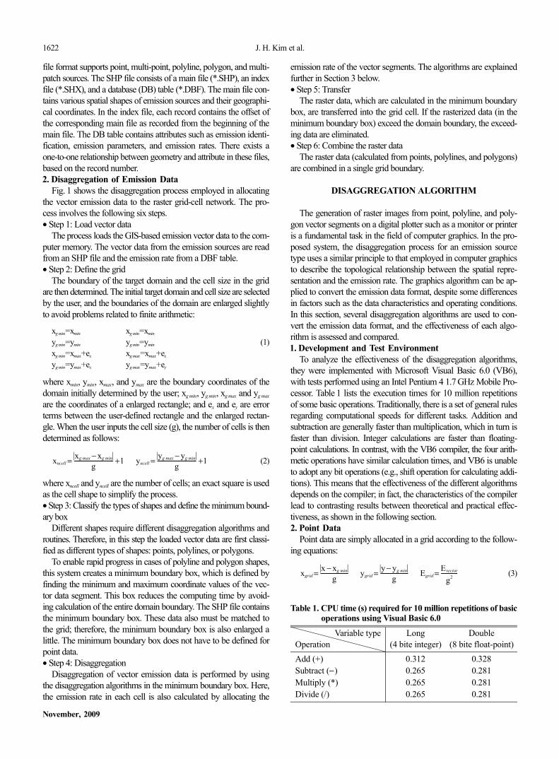
file format supports point, multi-point, polyline, polygon, and multi-patch sources. The SHP file consists of a main file (*.SHP), an indexfile (*.SHX), and a database (DB) table (*.DBF). The main file con-tains various spatial shapes of emission sources and their geographi-cal coordinates. In the index file, each record contains the offset ofthe corresponding main file as recorded from the beginning of themain file. The DB table contains attributes such as emission identi-fication, emission parameters, and emission rates. There exists aone-to-one relationship between geometry and attribute in these files,based on the record number.2. Disaggregation of Emission Data

Fig. 1 shows the disaggregation process employed in allocatingthe vector emission data to the raster grid-cell network. The pro-cess involves the following six steps.• Step 1: Load vector data

The process loads the GIS-based emission vector data to the com-puter memory. The vector data from the emission sources are readfrom an SHP file and the emission rate from a DBF table.• Step 2: Define the grid

The boundary of the target domain and the cell size in the gridare then determined. The initial target domain and cell size are selectedby the user, and the boundaries of the domain are enlarged slightlyto avoid problems related to finite arithmetic:

xg min=xmin xg min=xmin

yg min=ymin yg min=ymin (1)xg min=xmax+ex xg max=xmax+ex

yg min=ymax+ex yg max=ymax+ey

where xmin, ymin, xmax, and ymax are the boundary coordinates of thedomain initially determined by the user; xg min, yg min, xg max and yg max

are the coordinates of a enlarged rectangle; and ex and ey are errorterms between the user-defined rectangle and the enlarged rectan-gle. When the user inputs the cell size (g), the number of cells is thendetermined as follows:

(2)

where xncell and yncell are the number of cells; an exact square is usedas the cell shape to simplify the process.• Step 3: Classify the types of shapes and define the minimum bound-ary box

Different shapes require different disaggregation algorithms androutines. Therefore, in this step the loaded vector data are first classi-fied as different types of shapes: points, polylines, or polygons.

To enable rapid progress in cases of polyline and polygon shapes,this system creates a minimum boundary box, which is defined byfinding the minimum and maximum coordinate values of the vec-tor data segment. This box reduces the computing time by avoid-ing calculation of the entire domain boundary. The SHP file containsthe minimum boundary box. These data also must be matched tothe grid; therefore, the minimum boundary box is also enlarged alittle. The minimum boundary box does not have to be defined forpoint data.• Step 4: Disaggregation

Disaggregation of vector emission data is performed by usingthe disaggregation algorithms in the minimum boundary box. Here,the emission rate in each cell is also calculated by allocating the

emission rate of the vector segments. The algorithms are explainedfurther in Section 3 below.• Step 5: Transfer

The raster data, which are calculated in the minimum boundarybox, are transferred into the grid cell. If the rasterized data (in theminimum boundary box) exceed the domain boundary, the exceed-ing data are eliminated.• Step 6: Combine the raster data

The raster data (calculated from points, polylines, and polygons)are combined in a single grid boundary.

DISAGGREGATION ALGORITHM

The generation of raster images from point, polyline, and poly-gon vector segments on a digital plotter such as a monitor or printeris a fundamental task in the field of computer graphics. In the pro-posed system, the disaggregation process for an emission sourcetype uses a similar principle to that employed in computer graphicsto describe the topological relationship between the spatial repre-sentation and the emission rate. The graphics algorithm can be ap-plied to convert the emission data format, despite some differencesin factors such as the data characteristics and operating conditions.In this section, several disaggregation algorithms are used to con-vert the emission data format, and the effectiveness of each algo-rithm is assessed and compared.1. Development and Test Environment

To analyze the effectiveness of the disaggregation algorithms,they were implemented with Microsoft Visual Basic 6.0 (VB6),with tests performed using an Intel Pentium 4 1.7 GHz Mobile Pro-cessor. Table 1 lists the execution times for 10 million repetitionsof some basic operations. Traditionally, there is a set of general rulesregarding computational speeds for different tasks. Addition andsubtraction are generally faster than multiplication, which in turn isfaster than division. Integer calculations are faster than floating-point calculations. In contrast, with the VB6 compiler, the four arith-metic operations have similar calculation times, and VB6 is unableto adopt any bit operations (e.g., shift operation for calculating addi-tions). This means that the effectiveness of the different algorithmsdepends on the compiler; in fact, the characteristics of the compilerlead to contrasting results between theoretical and practical effec-tiveness, as shown in the following section.2. Point Data

Point data are simply allocated in a grid according to the follow-ing equations:

(3)

xncell = xg max − xg min

g---------------------------- +1 yncell =

yg max − yg min

g---------------------------- +1

xgrid = x − xg min

g-------------------- ygrid =

y − yg min

g-------------------- Egrid =

Evector

g2------------

Table 1. CPU time (s) required for 10 million repetitions of basicoperations using Visual Basic 6.0

Variable typeOperation

Long(4 bite integer)

Double(8 bite float-point)

Add (+) 0.312 0.328Subtract (−) 0.265 0.281Multiply (*) 0.265 0.281Divide (/) 0.265 0.281



where x and y are the point coordinates of the vector data, xgrid andygrid are the coordinates of a point source matched with the grid, Evector

is the emission rate (kg/yr) of the vector data, and Egrid is the emis-sion rate (kg/yr·m2) of the contained grid. In point disaggregation,additional calculations of the emission rate allocation and boundarybox are not required. In the case of Korea, there exist about 3,000point sources for toxic chemical emission inventories. The comput-ing time required for 3,000 points sources is about 0.14µs, posing noproblem for the disaggregation process.3. Line Data

Existing algorithms for line disaggregation can be broadly clas-sified into three groups: incremental algorithms, packing algorithms,and algorithms that employ the symmetry principle. The first in-cremental algorithm was devised by Bresenham [17]. This well-known algorithm uses only integer arithmetic, which removes realnumbers and division operations in the computation to ensure theprompt generation of line segments. Pitteway [24] proposed a for-mulation, known as the midpoint technique, which differed fromBresenham’s incremental algorithm and was subsequently adaptedby Aken [16] and Kappel [22], among others.

Many subsequent researchers have proposed methods for pack-ing the calculation steps to reduce the number of incremental steps.Wu and Rokne [30] developed the double-step method, which wasthen expanded to the multi-step technique [19]. The main idea behindthe multi-step technique is to choose one pattern (a set of points)

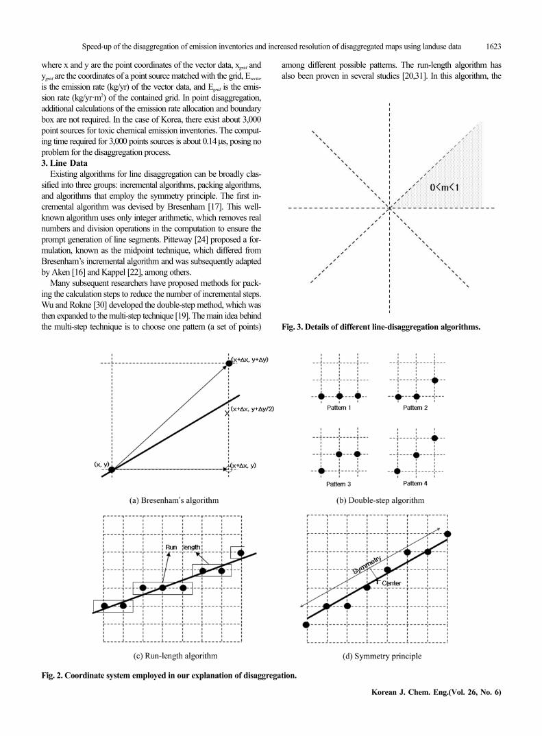
Fig. 2. Coordinate system employed in our explanation of disaggregation.

Fig. 3. Details of different line-disaggregation algorithms.

among different possible patterns. The run-length algorithm hasalso been proven in several studies [20,31]. In this algorithm, the


November, 2009

incremental step is reduced by determining the run-length.Gardner [18] proposed a new approach to speed up the line scan-

conversion process, based on the symmetry property of a line: thescan-converted line is symmetric about the center point of the line.The symmetry principle enables the calculation of only half of theline.

In performing line disaggregation, we tested three algorithms:Bresenham’s algorithm, the double-step method, and the run-lengthalgorithm employing the symmetry principle. We discuss the linedisaggregation problem in the first octant (slopes between 0 and 1)of the Cartesian coordinate system, as shown in Fig. 2. The algo-rithm is easily extended to other octants. The disaggregation algo-rithms for lines are described below.• Bresenham’s algorithm

Fig. 3(a) shows the principle behind Bresenham’s algorithm. Weassume a starting point (x, y). In the first octant, there are two basicoptional moves in the raster grid field: the diagonal move (x+dx,y+dy) and the horizontal move (x+dx, y). The optional moves canbe approximated by the relative positions of the mid-point (x+dx,y+dy/2) and the line (bold line in Fig. 3(a)). The relative position isdetermined by testing the sign of a function known as a discrimi-nator.• Double-step method

The basic idea of the algorithm in the double-step method is toconsider two steps at a time (rather than one). If we have a drawnpixel (x, y), the next two pixels can be selected from four possiblefixed patterns, as shown in Fig. 3(b). In Bresenham’s algorithm,the sign of a discriminator predicts the pixel to be chosen at anystep. In contrast, the double-step method calculates the discrimina-tor for every two steps. Theoretically, calculations can be performedat almost twice the speed of that possible using Bresenham’s algo-rithm.• Run-length algorithm

A run is defined as a contiguous set of pixels with the same Xor Y coordinate. Consider a line from (x1, y1) to (x2, y2) on theraster grid field, where x2>y2. If we consider lines with slopes from1/2 to 1/3, the run-length must be 2 or 3, as shown in Fig. 3(c). Theline can be viewed as the series of the run. The calculation speedof this algorithm depends on the slope of the line.• Symmetry principle

Fig. 3(d) describes the symmetry principle of a line. The rasterpixel related to the vector line has a symmetric pixel pattern basedon the center of the line. This principle can be applied to the dis-aggregation in combination with other algorithms. Theoretically,this algorithm can almost double the calculation speed of the origi-nal disaggregation algorithm.

After using the above algorithms to find the cell crossed by theline, the emission rate in each cell is allocated as follows:

(4)

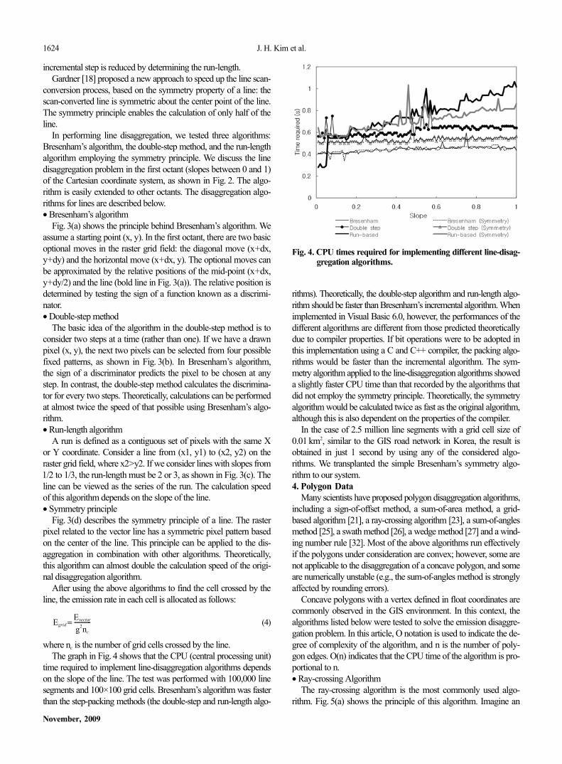
where nc is the number of grid cells crossed by the line.The graph in Fig. 4 shows that the CPU (central processing unit)

time required to implement line-disaggregation algorithms dependson the slope of the line. The test was performed with 100,000 linesegments and 100×100 grid cells. Bresenham’s algorithm was fasterthan the step-packing methods (the double-step and run-length algo-

rithms). Theoretically, the double-step algorithm and run-length algo-rithm should be faster than Bresenham’s incremental algorithm. Whenimplemented in Visual Basic 6.0, however, the performances of thedifferent algorithms are different from those predicted theoreticallydue to compiler properties. If bit operations were to be adopted inthis implementation using a C and C++ compiler, the packing algo-rithms would be faster than the incremental algorithm. The sym-metry algorithm applied to the line-disaggregation algorithms showeda slightly faster CPU time than that recorded by the algorithms thatdid not employ the symmetry principle. Theoretically, the symmetryalgorithm would be calculated twice as fast as the original algorithm,although this is also dependent on the properties of the compiler.

In the case of 2.5 million line segments with a grid cell size of0.01 km2, similar to the GIS road network in Korea, the result isobtained in just 1 second by using any of the considered algo-rithms. We transplanted the simple Bresenham’s symmetry algo-rithm to our system.4. Polygon Data

Many scientists have proposed polygon disaggregation algorithms,including a sign-of-offset method, a sum-of-area method, a grid-based algorithm [21], a ray-crossing algorithm [23], a sum-of-anglesmethod [25], a swath method [26], a wedge method [27] and a wind-ing number rule [32]. Most of the above algorithms run effectivelyif the polygons under consideration are convex; however, some arenot applicable to the disaggregation of a concave polygon, and someare numerically unstable (e.g., the sum-of-angles method is stronglyaffected by rounding errors).

Concave polygons with a vertex defined in float coordinates arecommonly observed in the GIS environment. In this context, thealgorithms listed below were tested to solve the emission disaggre-gation problem. In this article, O notation is used to indicate the de-gree of complexity of the algorithm, and n is the number of poly-gon edges. O(n) indicates that the CPU time of the algorithm is pro-portional to n.• Ray-crossing Algorithm

The ray-crossing algorithm is the most commonly used algo-rithm. Fig. 5(a) shows the principle of this algorithm. Imagine an

Egrid = Evector

g2nc

------------

Fig. 4. CPU times required for implementing different line-disag-gregation algorithms.



infinite line starting at point Q, then count the number of intersec-tions made by the line and the edges of the polygon. If the numberof intersections on either side of point Q is an odd number, point Qis inside the polygon PG. This algorithm successfully solves all kindsof polygons, in O(n) time. For implementation, some special situa-tions must be considered (e.g., point Q lying on one of the polygonedges, or the ray intersecting the polygon at a node).• Swath method

The swath algorithm uses the ray-crossing algorithm, but severalpre-processing procedures are required. The polygon is first dividedinto swaths, as shown in Fig. 5(b). This procedure is completed inO(nlogn) time. Each swath has at least two edges, with a maxi-mum of n−1 edges. Using a binary search, the swath is located forthe considered point in time O(logn); the ray-crossing method isthen applied to the polygon edges located in the swath. This algo-rithm is useful when more points must be matched against the samepolygon.• Winding number rule

The winding number accurately determines if a point is inside anon-simple closed polygon. It is performed by computing how many

times the polygon winds around the point. A point is outside onlywhen the polygon does not wind around the point at all (i.e., thewinding number is zero). This algorithm requires O(n) time.• Grid-based method

The grid-based method is suitable for a raster-based situation.The polygon is represented by a group of cells; thus, the algorithmrequires pre-processing for a vector-based situation. The polygonborder is first rasterized by the line-disaggregation algorithm (blackcircles in Fig. 5(d)). This is completed in time O(n). The inner orouter cells are then determined by various algorithms such as a seed-fill algorithm, a scan-line algorithm, or a border-start algorithm; thesealgorithms are explained in Fig. 5(d). The seed-fill algorithm (alsoknown as a ‘flood-fill algorithm’) plants a seed, and progressivelymore seeds are recursively planted around the first seed. Each newseed is responsible for finding the inner cell. The core function ofthe scan-line algorithm is detection of the spans of the scan-line lyingwithin the polygon, based on the following process. The algorithmidentifies the intersections of the scan-line with all the edges of thepolygon, sorts the intersections, and fills in all the pixels betweenpairs of intersections. The border-start algorithm operates by mov-

Fig. 5. Details of different polygon-disaggregation algorithms.


November, 2009

ing from the borders of the minimum boundary box in the left, right,down, or up directions, and then finds the outer cells until it encoun-ters the edge of the polygon.

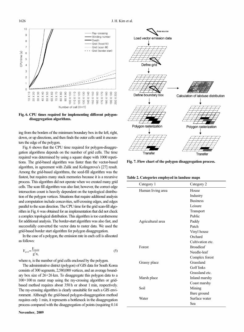
Fig. 6 shows that the CPU time required for polygon-disaggre-gation algorithms depends on the number of grid cells. The timerequired was determined by using a square shape with 1000 repeti-tions. The grid-based algorithm was faster than the vector-basedalgorithm, in agreement with Zalik and Kolingerova’s [27] result.Among the grid-based algorithms, the seed-fill algorithm was thefastest, but requires many stack memories because it is a recursiveprocess. This algorithm did not operate when we created many gridcells. The scan fill algorithm was also fast; however, the correct edgeintersection count is heavily dependent on the topological distribu-tion of the polygon vertices. Situations that require additional analysisand computation include concavities, self-crossing edges, and edgesparallel to the scan direction. The CPU time for the grid scan-fill algo-rithm in Fig.6 was obtained for an implementation that did not checka complex topological distribution. This algorithm is too cumbersomefor additional analysis. The border-start algorithm was also fast, andsuccessfully converted the vector data to raster data. We used thegrid-based border start algorithm for polygon disaggregation.

In the case of a polygon, the emission rate in each cell is allocatedas follows:

(5)

where ne is the number of grid cells enclosed by the polygon.The administrative district (polygon) of GIS data for South Korea

consists of 300 segments, 2,580,000 vertices, and an average bound-ary box size of 26×26 km. To disaggregate this polygon data to a100×100 m raster map using the ray-crossing algorithm or grid-based method requires about 350 h or about 1 min, respectively.The ray-crossing algorithm is clearly unsuitable for such a GIS envi-ronment. Although the grid-based polygon-disaggregation methodrequires only 1 min, it represents a bottleneck in the disaggregationprocess compared with the disaggregation of points (requiring 0.14

Egrid = Evector

g2ne

------------

Fig. 6. CPU times required for implementing different polygon-disaggregation algorithms.

Fig. 7. Flow chart of the polygon disaggregation process.

Table 2. Categories employed in landuse maps

Category 1 Category 2

Human living area HouseIndustryBusinessLeisureTransportPublic

Agricultural area PaddyPatchVinyl houseOrchardCultivation etc.

Forest BroadleafNeedle-leafComplex forest

Grassy place GrasslandGolf linksGrassland etc.

Marsh place Inland marshyCoast marshy

Soil MiningBare ground

Water Surface waterSea



µs) and polylines (1 s).

LANDUSE-SUPPORTED DISAGGREGATION METHOD

1. MethodologyTo increase spatial accuracy, we propose an advanced polygon-

disaggregation method (landuse-supported method). We assumedthat among the different landuse categories, toxic chemicals are onlyreleased in human living areas. In our case, the landuse map wasacquired from the Environmental Geographic Information System(http://egis.me.go.kr) managed by the Ministry of Environment,Korea. The landuse map consists of 23 categories, with a cell sizeof 30×30 m. The categories are listed in Table 2, with those cate-gories containing human living areas emphasized by bold type. Theadvanced method starts from the general polygon-disaggregationmethod (grid-based method) introduced in Section 2 and Fig. 1, towhich one process is added. Following definition of the boundary

box, the distribution ratio of the target landuse is calculated on eachgrid with reference to the landuse map. The disaggregation processis then performed with a spatial allocation of the emission rate ob-tained by the following improved form of Eq. (5):

(6)

where µ is the proportion of human living areas among the landusecategories.2. Disaggregated Map

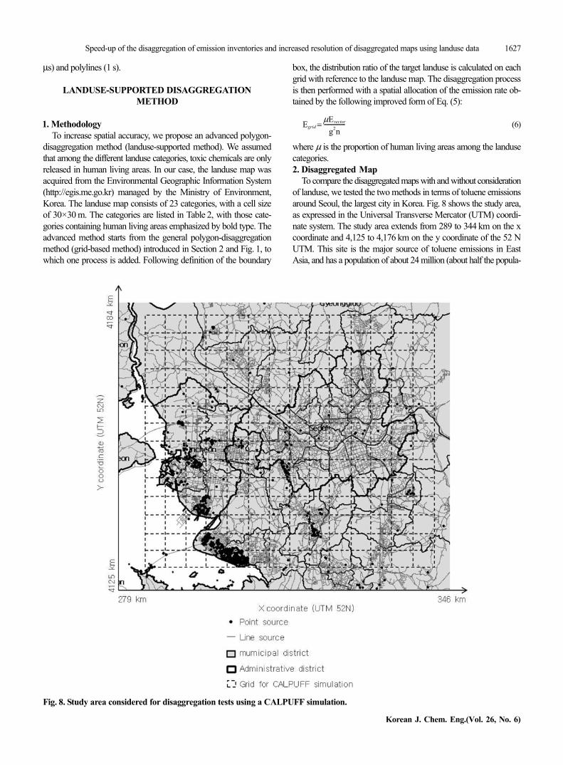
To compare the disaggregated maps with and without considerationof landuse, we tested the two methods in terms of toluene emissionsaround Seoul, the largest city in Korea. Fig. 8 shows the study area,as expressed in the Universal Transverse Mercator (UTM) coordi-nate system. The study area extends from 289 to 344 km on the xcoordinate and 4,125 to 4,176 km on the y coordinate of the 52 NUTM. This site is the major source of toluene emissions in EastAsia, and has a population of about 24 million (about half the popula-

Egrid = µEvector

g2n---------------

Fig. 8. Study area considered for disaggregation tests using a CALPUFF simulation.


November, 2009

tion of South Korea). The emission rate of toluene was obtainedfrom previous publications [33-35].

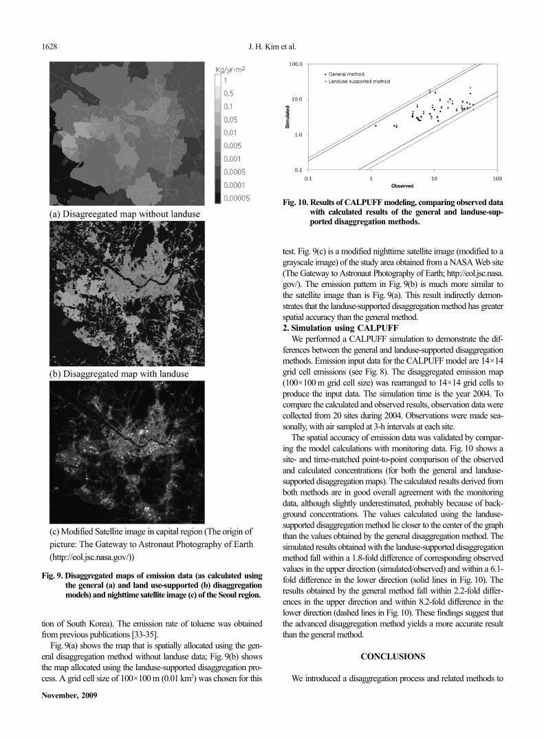
Fig. 9(a) shows the map that is spatially allocated using the gen-eral disaggregation method without landuse data; Fig. 9(b) showsthe map allocated using the landuse-supported disaggregation pro-cess. A grid cell size of 100×100 m (0.01 km2) was chosen for this

test. Fig. 9(c) is a modified nighttime satellite image (modified to agrayscale image) of the study area obtained from a NASA Web site(The Gateway to Astronaut Photography of Earth; http://eol.jsc.nasa.gov/). The emission pattern in Fig. 9(b) is much more similar tothe satellite image than is Fig. 9(a). This result indirectly demon-strates that the landuse-supported disaggregation method has greaterspatial accuracy than the general method.2. Simulation using CALPUFF

We performed a CALPUFF simulation to demonstrate the dif-ferences between the general and landuse-supported disaggregationmethods. Emission input data for the CALPUFF model are 14×14grid cell emissions (see Fig. 8). The disaggregated emission map(100×100 m grid cell size) was rearranged to 14×14 grid cells toproduce the input data. The simulation time is the year 2004. Tocompare the calculated and observed results, observation data werecollected from 20 sites during 2004. Observations were made sea-sonally, with air sampled at 3-h intervals at each site.

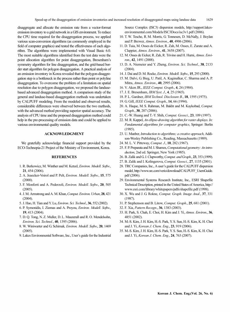
The spatial accuracy of emission data was validated by compar-ing the model calculations with monitoring data. Fig. 10 shows asite- and time-matched point-to-point comparison of the observedand calculated concentrations (for both the general and landuse-supported disaggregation maps). The calculated results derived fromboth methods are in good overall agreement with the monitoringdata, although slightly underestimated, probably because of back-ground concentrations. The values calculated using the landuse-supported disaggregation method lie closer to the center of the graphthan the values obtained by the general disaggregation method. Thesimulated results obtained with the landuse-supported disaggregationmethod fall within a 1.8-fold difference of corresponding observedvalues in the upper direction (simulated/observed) and within a 6.1-fold difference in the lower direction (solid lines in Fig. 10). Theresults obtained by the general method fall within 2.2-fold differ-ences in the upper direction and within 8.2-fold difference in thelower direction (dashed lines in Fig. 10). These findings suggest thatthe advanced disaggregation method yields a more accurate resultthan the general method.

CONCLUSIONS

We introduced a disaggregation process and related methods to

Fig. 9. Disaggregated maps of emission data (as calculated usingthe general (a) and land use-supported (b) disaggregationmodels) and nighttime satellite image (c) of the Seoul region.

Fig. 10. Results of CALPUFF modeling, comparing observed datawith calculated results of the general and landuse-sup-ported disaggregation methods.



disaggregate and allocate the emission rate from a vector-formatemission inventory to a grid network in a GIS environment. To reducethe CPU time required for the disaggregation process, we appliedvarious scan-conversion algorithms (as commonly employed in thefield of computer graphics) and tested the effectiveness of each algo-rithm. The algorithms were implemented with Visual Basic 6.0.The most suitable algorithms identified from the test data were thepoint allocation algorithm for point disaggregation, Bresenham’ssymmetry algorithm for line disaggregation, and the grid-based bor-der start algorithm for polygon disaggregation. A practical analysis ofan emission inventory in Korea revealed that the polygon-disaggre-gation step is a bottleneck in the process rather than point or polylinedisaggregation. To overcome the problem of a limitation on spatialresolution due to polygon disaggregation, we proposed the landuse-based advanced disaggregation method. A comparison study of thegeneral and landuse-based disaggregation methods was undertakenby CALPUFF modeling. From the modeled and observed results,considerable differences were observed between the two methods,with the advanced method providing superior spatial accuracy. Theanalysis of CPU time and the proposed disaggregation method couldhelp in the pre-processing of emission data and could be applied tovarious environmental quality models.

ACKNOWLEDGMENT

We gratefully acknowledge financial support provided by theECO-Technopia-21 Project of the Ministry of Environment, Korea.

REFERENCES

1. R. Berkowicz, M. Winther and M. Ketzel, Environ. Modell. Softw.,21, 454 (2006).

2. A. Jeaecker-Voirol and P. Pelt, Environ. Modell. Softw., 15, 575(2000).

3. F. Monforti and A. Pederzoli, Environ. Modell. Softw., 20, 505(2005).

4. J. M. Armstrong and A. M. Khan, Comput. Environ. Urban, 28, 421(2004).

5. J. Hao, H. Tian and Y. Lu, Environ. Sci. Technol., 36, 552 (2002).6. P. Symonidis, I. Ziomas and A. Proyou, Environ. Modell. Softw.,

19, 413 (2004).7. D. Q. Tong, N. Z. Muller, D. L. Mauzerall and R. O. Mendelsohn,

Environ. Sci. Technol., 40, 1395 (2006).8. W. Winiwarter and G. Schimak, Environ. Modell. Softw., 20, 1469

(2005).9. Lakes Environmental Software, Inc., User’s guide for the Industrial

Source Complex (ISC3) dispersion models, http://support.lakes-environmental.com/Models/ISC3Docs/isc3v1.pdf (2006).

10. T. W. Tesche, R. M. Morris, G. Tonnesen, D. McNally, J. Boylanand P. Brewer, Atmos. Environ., 40, 4906 (2006).

11. D. Tuia, M. Osses de Eicker, R. Zah, M. Osses, E. Zarate and A.Clappier, Atmos. Environ., 41, 3658 (2007).

12. M. Osses de Eicker, R. Zah, R. Trivino and H. Hurni, Atmos. Envi-ron., 42, 1491 (2008).

13. D. A. Niemeier and Y. Zheng, Environ. Sci. Technol., 38, 2133(2004).

14. J. Dai and D. M. Rocke, Environ. Modell. Softw., 15, 293 (2000).15. M. Dalvi, G. Bieg, U. Patil, A. Kaginalkar, C. Sharma and A. P.

Mitra, Atmos. Environ., 40, 2995 (2006).16. V. Aken JR., IEEE Comput. Graph., 4, 24 (1984).17. J. E. Bresenham, IBM Syst. J., 4, 25 (1965).18. P. L. Gardner, IBM Technol. Disclosure B., 18, 1595 (1975).19. G. Gill, IEEE Comput. Graph., 14, 66 (1994).20. A. Haque, M. S. Rahman, M. Bakht and M. Kaykobad, Comput.

Graph., 30, 207 (2006).21. C.-W. Huang and T.-Y. Shih, Comput. Geosci., 23, 109 (1997).22. M. R. Kappel, An ellipse-drawing algorithm for raster displays. In:

Fundamental algorithms for computer graphics, Springer: Berlin(1985).

23. U. Manber, Introduction to algorithms; a creative approach, Addi-son-Wesley Publishing Co., Reading, Massachusetts (1989).

24. M. L. V. Pitteway, Comput. J., 10, 282 (1967).25. F. P. Preparata and M. I. Shamos, Computational geometry: An intro-

duction, 2nd ed. Springer, New York (1985).26. B. Zalik and G. J. Clapworthy, Comput. and Graph., 23, 353 (1999).27. B. Zalik and I. Kolingerova, Comput. Geosci., 27, 1135 (2001).28. TRC Companies, Inc., A user’s guide for the CALPUFF dispersion

model, http://www.src.com/verio/download/CALPUFF_UsersGuide.pdf (2006).

29. Environmental Systems Research Institute, Inc., ESRI ShapefileTechnical Description, printed in the United States of America, http://www.esri.com/library/whitepapers/pdfs/shapefile.pdf (1998).

30. X. Wu and J. G. Rokne, Comput. Graph. Image Anal., 37, 331(1987).

31. P. Stephenson and B. Litow, Comput. Graph., 25, 681 (2001).32. F. Xia, Pattern Recogn., 36, 1383 (2003).33. H. Park, S. Chah, E. Choi, H. Kim and J. Yi, Atmos. Environ., 36,

4851 (2002).34. M.-S. Kim, J. H. Kim, H.-S. Park, Y. S. Sun, H.-S. Kim, K. H. Choi

and J. Yi, Korean J. Chem. Eng., 23, 919 (2006).35. M.-S. Kim, J. H. Kim, H.-S. Park, Y. S. Sun, H.-S. Kim, K. H. Choi

and J. Yi, Korean J. Chem. Eng., 24, 763 (2007).

Documents

Speed-up of the disaggregation of emission inventories and ... · from an SHP file and the emission rate from a DBF table. • Step 2: Define the grid ... they were implemented with