NBER WORKING PAPER SERIES

SPIDERS AND SNAKES:OFFSHORING AND AGGLOMERATION IN THE GLOBAL ECONOMY

Richard BaldwinAnthony Venables

Working Paper 16611http://www.nber.org/papers/w16611

NATIONAL BUREAU OF ECONOMIC RESEARCH1050 Massachusetts Avenue

Cambridge, MA 02138December 2010

This paper is a revised and retitled version of Baldwin and Venables (2010). Thanks to two anonymousreferees, Bob Staiger and participants in seminars at Oxford and Princeton, conferences in Boston(NBER Summer Institute), Villars (CEPR), Rome (European Research Workshop in InternationalTrade), Osaka (Asia Pacific Trade Seminar), Jonkoping (European Regional Science Association)and Denver (ASSA). The views expressed herein are those of the authors and do not necessarily reflectthe views of the National Bureau of Economic Research.

NBER working papers are circulated for discussion and comment purposes. They have not been peer-reviewed or been subject to the review by the NBER Board of Directors that accompanies officialNBER publications.

© 2010 by Richard Baldwin and Anthony Venables. All rights reserved. Short sections of text, notto exceed two paragraphs, may be quoted without explicit permission provided that full credit, including© notice, is given to the source.

Spiders and snakes: offshoring and agglomeration in the global economyRichard Baldwin and Anthony VenablesNBER Working Paper No. 16611December 2010, Revised December 2012JEL No. F13,F29

ABSTRACT

Global production sharing is determined by international cost differences and frictions related to thecosts of unbundling stages spatially. The interaction between these forces depends on engineeringdetails of the production process with two extremes being ‘snakes’ and ‘spiders’. Snakes are processeswhose sequencing is dictated by engineering; spiders involve the assembly of parts in no particularorder. This paper studies spatial unbundling as frictions fall, showing that outcomes are very differentfor snakes and spiders, even if they share some features. Both snakes and spiders have in commona property that lower frictions produce discontinuous location changes and ‘overshooting’. Parts maymove against their comparative costs because of proximity benefits, and further reductions in frictionslead these parts to be ‘reshored’. Predictions for trade volumes and the number of fragmented stagesare quite different in the two cases. For spiders, a part crosses borders at most twice; the value of tradeincreases monotonically as frictions fall, except when the assembler relocates and the direction ofparts trade is reversed. For snakes the volume of trade and number of endogenously determined stages isbounded only by the fragmentation of the underlying engineering process, and lower frictions monotonicallyincrease trade volumes.

Richard BaldwinCigale 21010 LausanneSWITZERLANDand CEPRand also NBERrbaldwin@cepr.org

Anthony VenablesDepartment of EconomicsUniversity of OxfordManor Road BuildingManor RoadOxford OX1 3UQ, United Kingdomand CEPRtony.venables@economics.ox.ac.uk

1

1. Introduction

An ever finer division of labour has long been associated with economic progress. One step forward came as the steam revolution made it economical to produce goods far from consumers. Yet even as this first spatial unbundling (production unbundled from consumers) dispersed production globally, manufacturing clustered locally in factories and industrial districts to reduce coordination costs. A second step was triggered by the information and communications technology (ICT) revolution that massively lowered the cost of organising complex activities over distances. Advances in telecommunications and computing transformed information management and this in turn transformed the organisation of group-work across space. Stages of production that previously were performed in close proximity – within walking distance to facilitate face-to-face coordination of innumerable small glitches – can now be dispersed without an enormous drop in efficiency or timeliness. More recently, this second unbundling has spread from factories to offices, resulting in both the outsourcing and offshoring of service-sector jobs.

Numerous examples serve to illustrate the pervasiveness of unbundling. The “Swedish” Volvo S40 has an air-conditioner made in France, the headrest and seat warmer made in Norway, the fuel and brake lines in England, the hood latch cable in Germany, and so on. Some parts are even made in Sweden (airbag and seat beats).1 In auto-production unbundling is sometimes ‘modularised’, with parts coming together for assembly into a module which is then shipped whole to final assembly plants (Frigant and Lung 2002). For example, US car seats are typically assembled domestically in a plant within one hour of the final auto assembly plant. While there are virtually no US imports of complete car seats, imports of seat parts (mainly from China) amount to $5 billion annually (Klier and Rubinstein 2009).

The first large-scale unbundling of manufacturing processes started in the mid-1980s and took place over short distances; the Maquiladora programme created ‘twin plants’ along the US-Mexico border. Although the programme started in 1965, it only boomed in the 1980s with employment growing at 20% annually from 1982 to 1989 (Dallas Fed 2002, Feenstra and Hanson 1996). Another production unbundling started in East Asia at about the same time and for the same reasons. In Europe, the unbundling was stimulated first by the EU accession of Spain and Portugal in 1986, and then by the emergence of Central and Eastern European nations from the early 1990s. While offshoring from high-wage economies continues, the reverse process – so-called ‘reshoring’ – is also observed (Wu and Zhang 2011, Shirkin et al 2011). The phenomenon is too new to have generated much research but examples abound. General Electric has moved some of its appliance manufacturing from China to Kentucky, and NCR is shifting its production of ATM machines from China, India, and Hungary back to a facility located in Georgia (Collins 2010, Davidson 2010).

Unbundling has been centre stage in much recent international trade research. There have been important empirical studies charting the rise of trade in parts and components (Ng and Yeats 1999, Hummels, Ishii and Yi 2001, Ando and Kimura 2005, Kimura, Takahashi and Hayakawa 2007). However, formal measurement has been problematic since trade data does not make clear what goods are input to other goods, and analyses based on input-output tables are at too high a level of aggregation to capture the level of detail suggested by industry examples (Johnson and

1 Headquarters and some assembly are in Sweden, although the company is now owned by the Zhejiang Geely Holding Group.

2

Noguera 2012). Analytical work has taken a variety of approaches. Much of the focus has been on taking simple characterisations of the technology of unbundling and drawing out the general equilibrium implications for trade and wages (Yi 2003, Grossman and Rossi-Hansberg 2008, Markusen and Venables 2007, Baldwin and Robert-Nicoud 2010). Others have linked it to multinational activity (Helpman 1984, Fujita and Thisse 2006) and have placed it in the wider context of the organisation of firms (Helpman 2006).

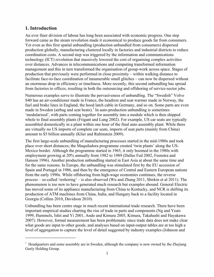
This paper focuses on quite different aspects. We take seriously the fact that technology – the engineering of the production process – dictates the way in which different stages of production are linked, and study the implications of this for unbundling.2 Possibilities are illustrated in Figure 1. Each cell is a stage at which value is added to a product that ends up as final consumption good; each arrow is a physical movement of a part, component, or the good itself. These may be movements within a country (possibly within a plant), or may be unbundled movements between plants in different countries.

Figure 1: Spiders and snakes

There are two quite different configurations. One we refer to as the spider: multiple limbs (parts) coming together to form a body (assembly), which may be the final product itself or a component (such as a module in the auto-industry). The other is the snake: the good moving in a sequential manner from upstream to downstream with value added at each stage.3 Most production processes are complex mixtures of the two. Cotton to yarn to fabric to shirts is a snake like process, but adding the buttons is a spider. Silicon to chips to computers is snake like, but much of value added in producing a computer is spider-like final assembly of parts from different sources.

2 Some management literature discusses this interaction, e.g. Sako (2005). 3 Dixit and Grossman (1982) analyse multi-stage production, but the order in which stages are performed is immaterial. Levine (2010) and Costinot et al (2011) study the implications of a snake in which mistakes can occur at each stage.

 

Final assembly

Part

Part

Part

Componentassembly

Part

Part

Part

VA VA VA VA

3

In production processes like those illustrated in the diagram the location of any one element depends on the location of others. We focus on ‘unbundling costs’ that occur when an arrow on the figure crosses an international boundary. They are likely to comprise the costs of coordination and management as well as direct shipping costs.4 These unbundling costs create centripetal forces binding related stages together. Firms seek to be close to other firms with which they transact, this depending on the technology of the product; it is different for snakes (each stage linked to an upstream and a downstream stage) than for spiders (each part linked only to assembly, but assembly linked to many parts). But there are also centrifugal forces that encourage dispersed production of different stages. For example, different stages have different factor intensities which create international cost differences and incentives to disperse. There is a tension between comparative costs creating the incentive to unbundle, and co-location or agglomeration forces binding stages of production together.

The paper analyses the interaction of these forces and shows how they determine the location of different parts of a value chain. We look at the efficient location of these stages when decisions are taken by a single cost-minimising agent, and also at outcomes when stages are controlled by independent decision takers. In the cost-minimising case the extent of offshoring and the volume of trade are discontinuous and non-monotonic functions of unbundling costs. If unbundling costs fall through time there are periods in which offshoring proceeds slowly, punctuated by periods of rapid change when a key production stage (such as assembly) relocates, taking many parts producers with it. Interactions between comparative advantage and co-location forces produce a systematic tendency for offshoring to ‘overshoot’ compared to predictions based purely on comparative production costs. An inevitable consequence of overshooting is ‘reshoring’; as ICT advances continue to weaken co-location forces, some offshored parts production moves back to its low-cost location. If the location of each stage of production is determined by independent decision takers then coordination failures mean that outcomes may not minimise costs. There may be multiple equilibria and locational hysteresis.

Our results highlight the fact that offshoring is unlikely to be a continuous process. As key stages relocate so other stages also move, perhaps against their comparative production costs; major parts of an industrial sector relocate in a discontinuous manner. These issues have arisen in earlier work on inter-industry linkages (e.g. Venables 1996, Fujita et al 1999) but in a stylised Dixit-Stiglitz structure of symmetric firms producing differentiated products. The present paper moves significantly beyond this work, with detailed focus on the heterogeneity between different stages of the chain and the interplay between these stages.

The remainder of the paper develops models of the spider and the snake in a two-nation setting (nations N and S), looking first at the spider. The economic setting is kept as simple as possible yet, despite this simplicity, interactions among stage-specific comparative advantage and stage-specific unbundling costs produce a surprisingly rich gallery of offshoring processes. The questions we address are: which stages are produced in N, which are produced in S, and how does this balance change during a process of globalisation? While the spider and snake give rise to different outcomes, there are a number of general implications that we draw out in concluding comments.

4 And costs associated with length and variability of time in transit, Harrigan and Venables (2006).

4

2. The spider

Throughout this section (spider) and the next (snake), the setting is a world of two countries, N and S, and we assume that all demand for the final product is in N.5 Production of the single final good requires a range of parts (intermediate inputs) that can be produced in N or S, and we assume production costs differ between countries part by part. Dispersing parts production across countries is costly, so a tension arises between unbundling production to reduce factor costs, and bundling it to reduce coordination and shipping costs.

The spider is a production process where separate parts are assembled into the final good.6 Parts are indexed by y Y. Unit production costs of all parts are unity if they are produced in N and

b(y) if produced in S, where bybb )( and bb 1 . This means that S has comparative advantage in parts with b < 1, and N has it in those with b > 1. Although it never enters the formal analysis, it is convenient to refer to S as labour-abundant, N as capital-abundant, parts with b(y) < 1 as labour-intensive, and those with b(y) >1 as capital-intensive.

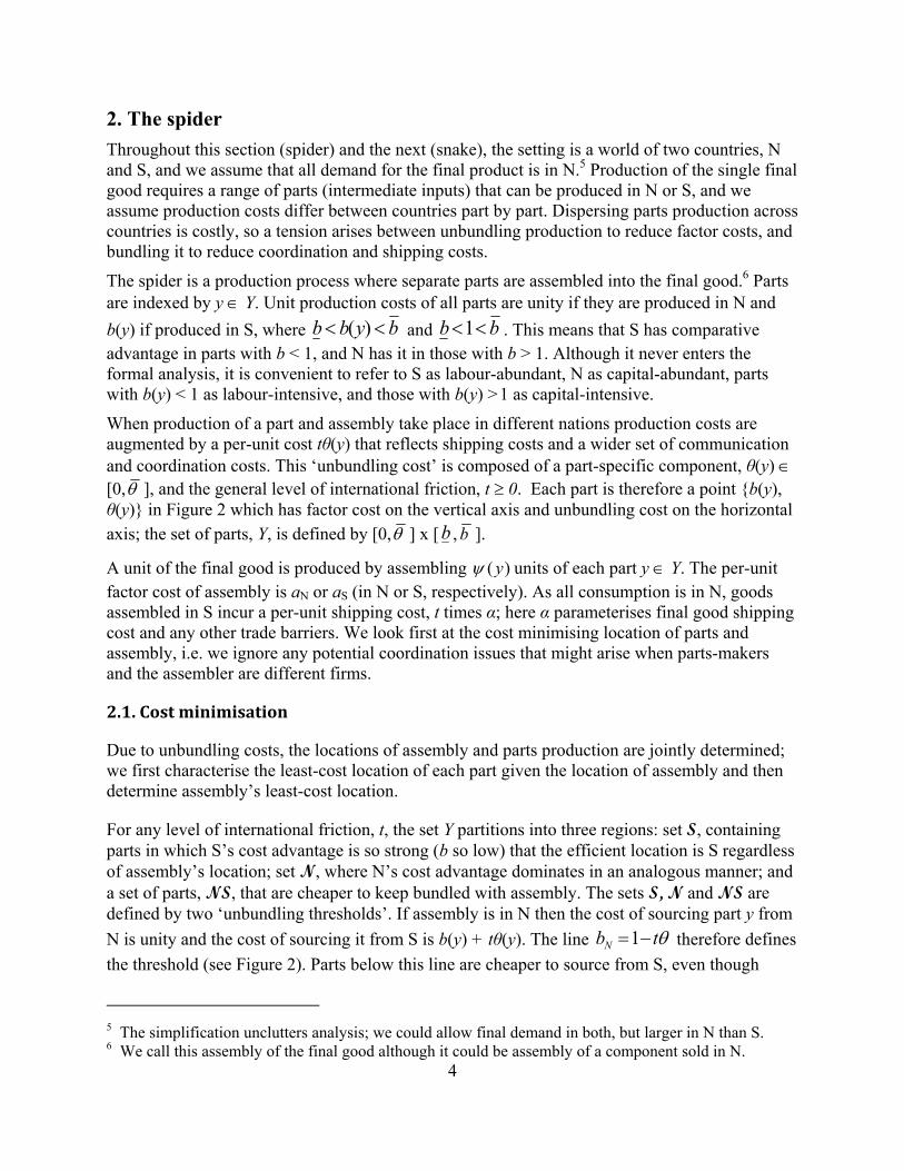
When production of a part and assembly take place in different nations production costs are augmented by a per-unit cost tθ(y) that reflects shipping costs and a wider set of communication and coordination costs. This ‘unbundling cost’ is composed of a part-specific component, θ(y) [0, ], and the general level of international friction, t 0. Each part is therefore a point {b(y), θ(y)} in Figure 2 which has factor cost on the vertical axis and unbundling cost on the horizontal axis; the set of parts, Y, is defined by [0, ] x [b , b ].

A unit of the final good is produced by assembling )( y units of each part y Y. The per-unit factor cost of assembly is aN or aS (in N or S, respectively). As all consumption is in N, goods assembled in S incur a per-unit shipping cost, t times α; here α parameterises final good shipping cost and any other trade barriers. We look first at the cost minimising location of parts and assembly, i.e. we ignore any potential coordination issues that might arise when parts-makers and the assembler are different firms.

2.1.Costminimisation

Due to unbundling costs, the locations of assembly and parts production are jointly determined; we first characterise the least-cost location of each part given the location of assembly and then determine assembly’s least-cost location.

For any level of international friction, t, the set Y partitions into three regions: set S, containing parts in which S’s cost advantage is so strong (b so low) that the efficient location is S regardless of assembly’s location; set N, where N’s cost advantage dominates in an analogous manner; and a set of parts, NS, that are cheaper to keep bundled with assembly. The sets S, N and NS are defined by two ‘unbundling thresholds’. If assembly is in N then the cost of sourcing part y from

N is unity and the cost of sourcing it from S is b(y) + tθ(y). The line tbN 1 therefore defines

the threshold (see Figure 2). Parts below this line are cheaper to source from S, even though

5 The simplification unclutters analysis; we could allow final demand in both, but larger in N than S. 6 We call this assembly of the final good although it could be assembly of a component sold in N.

5

assembly is in N; parts above the line are sourced from N. Likewise tbS 1 defines the

unbundling threshold when assembly is in S. Parts above Sb (set N) are most efficiently sourced

from N, and those below are sourced most cheaply from S.

Figure 2. Parts production costs and unbundling costs

The threshold definitions and Figure 2 give the location of parts production, conditional on the location of assembly and t. Notice that co-location with assembly is less important relative to productions costs when t is small, i.e. lowering the general level of international friction, t, makes N and S larger but NS smaller. Summarising:

Proposition 1: Location of parts, given assembly’s location.

i) If t = 0, parts y with b b(y) > 1 are produced in N; those with b b(y) < 1 are produced in S.

ii) If t > 0, there is a set of parts, NS, that co-locate with assembly. iii) As t → ∞ all parts co-locate with assembly (N and S disappear). iv) As t falls some parts relocate away from assembly in line with comparative production

costs (NS shrinks); at t = 0, NS disappears. v) Parts cross borders at most twice (once directly and once embodied in the final good).

Given proposition 1, the cost-minimising location of assembly is found by comparing total costs

b

b

b

b S = 1 + tθ

bN = 1 - tθ

S

N

NS

1 N: set of parts produced in N when assembly is in N or in S.S: set of parts produced in S when assembly is in N or in S.NS: set of parts produced in N if assembly is in N, in S if assembly is in S.

0

6

when assembly is in N with costs when it is in S, with parts location determined by the sets N, S and NS. Denoting total costs when assembly is in N or S by CN , CS, we have:

.)()()()(1

,)()()()(

dyyybdyyyttaC

dyyytybdyyaC

yySS

yyNN

NSSN

SNSN

(1)

The first term on the right hand side of each equation is unit assembly cost plus, if assembly is in S, the cost tα of getting the assembled product to consumers. The second and third terms are the cost of producing parts in N and S respectively with the limits of integration reflecting cost-minimising parts location. Assembly occurs in N unless CN - CS > 0, where:

( ) ( ) ( ) ( ) 1 ( ) ( )

N S N S

y y y

C C a a t

t y y dy y y dy b y y dy

S N NS

(2)

The forces determining assembly’s location are grouped into the three bracketed terms. The first is S’s trade-cost-adjusted comparative advantage in assembly. The second is the difference in parts’ unbundling costs; these costs are paid on S parts when assembly is in N, but on N parts when it is in S. The third term reflects the difference in production costs for parts in NS which are produced in either N or S, depending on the location of assembly.

An increase in any term tends to favour assembly in S, so the sign and magnitude of the terms and the way they change with t are the focus of our analysis. The first term’s size and sign has two determinants: S’s comparative advantage in assembly (aN - aS), and the final-good shipping costs t. If aN - aS < 0, the term is always negative and thus always favours assembly in N; if aN - aS > 0, then it is negative for high t and positive for low t. The second term is the product of t and integrals depending on the sizes of sets S and N, the shares of parts in assembly, )( y , and the unbundling cost intensity of the parts, θ(y). The term tends to be positive when comparative advantage in parts is skewed towards S, i.e. set S is large relative to set N in which case assembly in N incurs high unbundling costs. 7 Falling t affects the size of both S and N (Proposition 1.iii) and also reduces the magnitude of the second term directly, with it disappearing at t = 0. The third term’s sign is also ambiguous. Shifting production of parts in NS from N to S lowers the factor-costs of parts in the range [bN,1] but raises factor costs for parts in [1, bS]. The term is positive if the former outweighs the latter. Regardless of its sign, the third term is zero at t = 0 since NS shrinks to zero (Proposition 1.iv).

Proposition 1 and equation (2) combine to give two propositions characterising the location of assembly and parts production. The first covers the case in which comparative advantage in assembly resides in S, and the second the case in which it is in N.

7 In terms of Figure 2 comparative advantage in parts is skewed towards S when [ b ,b ] is low compared to 1 (as shown) but skewed towards N if the range is high compared to 1.

7

Proposition 2: S has comparative advantage in assembly.

If aN - aS > 0 then: i) Assembly takes place in N at very high values of t, and in S at low values of t. ii) There is at least one switch point at which assembly moves from N to S.

If the switch point is unique (at t’) then reducing t brings: iii) a. For t > t’, an increase in S, the set of parts produced in S and exported to N.

b. At t = t’, assembly and production of parts in set NS moves from N to S. c. For t < t’, reduction in NS implying a ‘reshoring’ process in which parts which

have ‘overshot’ move back from S to N. iv) Associated with changing location of production, reducing t brings:

a. For t > t’, an increase in the volume of trade in parts. b. At t = t’ trade in the final product commences; the composition of parts trade

changes and its volume may increase or decrease. c. For t < t’, reshoring increases the volume of trade in parts.

v) The share of value added produced in S is maximised at t = t’, once assembly and parts in set NS are in S.

Proof of part (i) comes from inspection of equation (2). As t → ∞, CN - CS becomes negative since the first term in (2) limits to negative infinity, the second term disappears as S and N shrink to null sets (Proposition 1), and the third term remains finite. Thus, regardless of the third term’s sign, assembly and production of all parts takes place in N, co-locating with final demand. At the other extreme, when t = 0, the second and third terms disappear, i.e. CN - CS = aN - aS, so S’s comparative advantage in assembly dominates; parts with b > 1 are in N and the rest are in S. Proof of part iii.b follows from this, as CN - CS is negative at high t and positive at low t. Propositions iii.a and iii.c follow from the fact that N and S expand as NS shrinks with falling t (Proposition 1iii). Parts iv and v follow similarly.

Proposition 3: N has comparative advantage in assembly.

If aN - aS < 0 then: i) Assembly takes place in N at very high and very low values of t. ii) There may be pairs of switch points where assembly and parts in NS switch from N

to S and then back from S to N. Each switch is associated with overshooting. iii) If there are no switch points then reductions in t increase the share of production in S

and the volume of trade. If there is a single pair of switch points (t’, t’’) then

vi) a. The share of value added produced in S is maximised at the upper switch point, once assembly and parts in set NS are in S. b. Reducing t increases the volume of trade except at a switch point at which

assembly and parts in NS switch from S to N.

Proof of part (i) comes from inspection of equation (2), noting the two points we showed above: CN - CS turns negative as t approaches infinity (so assembly is in N for high t), and CN - CS equals aN - aS < 0 at t = 0. The possibility of a pair of switch points can be shown by considering an

8

extreme example where comparative advantage in parts is so heavily skewed towards S that it can be cheaper to move assembly to S (thus saving unbundling costs on importing parts from S) despite the extra factor and trade costs of undertaking assembly in the ‘wrong’ region. For example in the extreme case that S has comparative advantage in all parts (i.e. b = 1 >b ), (2)’s second term is positive for all intermediate values of t since N is always empty. The third term is also positive for intermediate t since shifting parts production from N to S always lowers direct production costs. This means that, if aN - aS and are small enough, CN - CS could be positive for intermediate values of t as the strictly positive second and third term outweigh the negative first term. Parts (iii) and (iv) follow directly from the location of production.

Equalunbundlingcosts

In order to explore and illustrate overshooting and reshoring more fully, we now add structure that permits analytical solutions. The simplifications we assume are that all parts have the same unbundling costs, i.e. θ(y) = 1 for all y, and that parts are uniformly distributed on ],[ bb with

equal shares in assembly, i.e. (y) = 1 for all y. This collapses the two-dimensions of Y into one. Since the production process imposes no ordering on parts, we index them in order of S’s comparative advantage, taking each part’s b as the index. The unbundling thresholds are points

(scalars rather than lines as in Figure 2) and the sets N, NS, and S are intervals N = ],[ bbS , NS

= ],,[ SN bb and S = ],[ Nbb .

With equal-unbundling cost, equation (2) becomes:8

( ) ( ) 1 ( )

2S N

N S N S N S S N

b bC C a a t t b b b b b b

(3)

where unbundling thresholds, bS and bN, characterise the cost-minimising location of parts given the assembler’s location. It is easy to show that bS = 1 + t and bN = 1 - t, providing t is small enough for the unbundling points bS and bN to lie within [ b ,b ],9 while more generally bS =

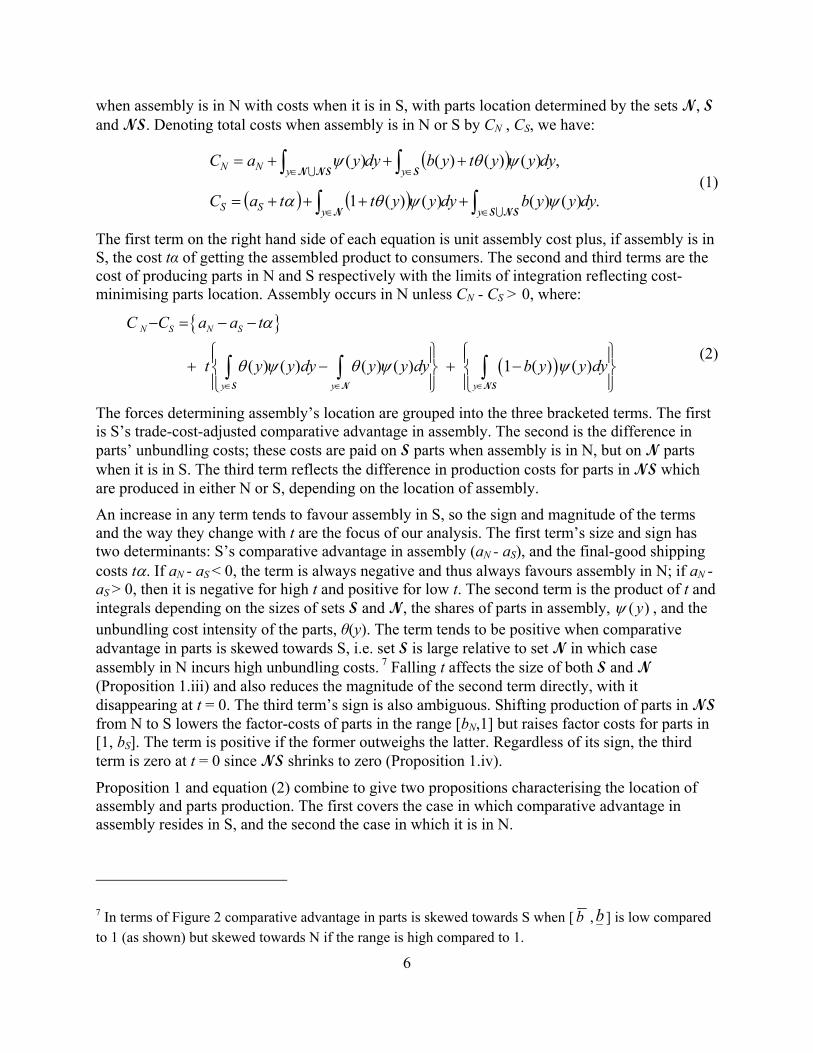
min[1+t,b ] and bN = max[1-t,b ], allowing for corner solutions. We illustrate how intervals N, S, and NS vary with the friction, t, on Figure 3 that has b on the vertical axis and t on the horizontal; the left and right panels are drawn, respectively, for the cases where S and N have comparative advantage in assembly.

The unbundling thresholds define three ranges of t (Figure 3). In range-I, both thresholds vary continuously with t (bS = 1 + t and bN = 1- t). In range-III, both thresholds are invariant to t (bS = b and bN =b ). In the intermediate range-II, one threshold is at its corner solution while the other

8 Integrals in (1) become

N

N

bb NNNN

bbNN bbtbbbbadbtbdbaC 2/)()()()(

S

S

bb SSS

bbSS bbbbttabdbdbttaC 2/)())(1()1( 22

9 First order conditions are CN/bN = bN + t – 1 = 0, CS/bS = bS – t – 1 = 0 for cost-minimising division

of parts provided that bS, bN ],[ bb .

9

varies with t.

To study how parts and assembly are offshored as frictions fall, we start with the case where S has comparative advantage in assembly. From Proposition 2, assembly and all parts-production is in N for sufficiently high t, but assembly and some parts are in S when t = 0. Parts’ location is determined by the usual N, S, and NS analysis; assembly switches location at the value of t at which CN – CS = 0. The expression for this is given in equation (3), and varies by range since the expressions for bS and bN vary by range. When parameters are such that the switching point falls in range-I (see Appendix 1), the switching point is:

'

2N Sa a

t

(4)

where β ≡ 1 - (b + b )/2 measures S’s cost advantage in parts, and is positive if the average cost

of producing parts in S, (b + b )/2, is less than it is in N (unity). Figure 3 and the following discussion assume β > 0, implying that bS takes its corner solution at a lower value of t than does bN.10 Expression (4) tells us that assembly’s switching point reflects the balance between S’s comparative advantage in parts and assembly, on the one hand, and the final-good shipping costs on the other. When S is very competitive in assembly (aN - aS is large) and in parts production ( is large), the switch occurs at a higher level of t for any given final-good shipping cost . Higher corresponds to a lower assembly switching point for given aN - aS and .

Figure 3: Cost minimising locations of parts and assembly.

S has comparative advantage in assembly N has comparative advantage in assembly

10 Analysis of the other case is analogous.

b

b

b

N

1

t

1

b 1 1b

I II III

t" t'

NS

S

b S = min [1+ t, ]

b N = max[1– t, ]

b

b

a N – aS < 0

b

b

b b S = min [1+ t, ]

b N = max[1– t, ]

N

1

tb 1 1 b

I II III

t’ t”

NS

S

b

b

1

aN – aS > 0

10

When the switch comes in range-I, the bold lines in the left panel of Figure 3 map out the associated cost-minimising location of parts. At high t, assembly is in N and all parts are bundled

with assembly regardless of comparative production costs, i.e. NS = ],[ bb . As t drops below the maximum cost differential, 1-b , parts with the lowest b are offshored to S and exported to N for assembly. At the switch point t’, assembly moves from N to S and parts in NS are moved to S en bloc to keep them bundled with assembly. Now N exports parts to S, and S exports final goods to N. Some of the parts in NS have higher production costs b > 1 (have ‘overshot’) and a reshoring process begins as t falls further. At t = 0, the allocation of production matches comparative advantage perfectly since assembly is in S along with all parts with b < 1.

The volume of trade in parts rises as t falls for any interval that does not include a switching point; whether assembly is in N or in S lower t enables location of parts to be determined by comparative cost advantage. But as assembly switches to S then trade volumes change discontinuously. Trade in final goods increases (from zero), but instead of parts in sets S being shipped to N, parts in N are shipped to S. The trade volume implications of this depend upon the relative size of N and S. Total trade is maximized at t = 0 where the size of N is maximised and final output is traded from S to N.

A more extreme form of offshoring and reshoring occurs when assembly’s switching point falls in range-III, at point t’’.11 The evolution of parts and assembly offshoring is illustrated by the small circles in Figure 3 (left panel). The whole industry – all parts and assembly – is in N at very high levels of friction, but once t falls below t’’, the whole industry is offshored to S. Reshoring of parts commences as t falls below b -1. The switching point is:

" ( ( ) ) /N St a a b b (5)

(appendix 1) so, as before, the switch comes at higher t’s when S’s cost advantages in parts and assembly are large and final-good shipping costs are low. Now, however, it also depends on the dispersion of S’s costs of parts production, namely b -b .

The case in which N has comparative advantage in assembly (aN - aS < 0) is described in Proposition 3 and illustrated in the right panel of Figure 3. Assembly takes place in N both at high and at low values of t. The double switching outcome is illustrated by the bold line on the right panel of Figure 3 with switches in range-III and range-I. There are three phases: when t is high, assembly stays close to the market because of costs of offshoring the final product; at intermediate t it is cost minimising to locate assembly in S in order to best use low-cost parts producers in S; at low t all elements – parts and assembly – locate according to their comparative production costs.

Sufficient conditions for this double switching to occur can be seen from equation (3). There is a switch point in range-III if CN – CS = 0 at some bt 1 . Setting bt 1 in (3), the condition is

that 01 bbbaaCC SNSN . While the first term is negative, this inequality will hold if S’s cost advantage in parts is large enough (β large), and/or the dispersion of costs of parts produced in S, i.e. b -b , is large. It is then efficient for assembly to be in S at this

11 Between these cases, switching occurs in range-II. See appendix 1 for parameters delineating for which the switch occurs in range-III.

11

intermediate level of t, in order to best access a large range of low cost parts produced in S. Appendix 1 analyses CN - CS across the three ranges in more detail.

Productioncosts,offshoringcosts,andshippingcosts

The analysis associated with Figure 3 assumes that parts differ in their production costs, b, but all face the same unbundling costs, θ(y) = 1. However, it is possible that parts’ unbundling costs vary systematically with their labour intensity, and in the working paper version we work through a case that allows for this, assuming unbundling costs are higher for more labour-intensive goods. There are two results. First, conditional on the location of assembly, a smaller range of parts is produced in S. Second, assembly takes place in S for a wider range of values of t. Thus, a consequence of it being more expensive to unbundle labour-intensive parts is that more offshoring may take place. The intuition is that it is more expensive to access S’s cost advantage through unbundling parts, and consequently more efficient to move assembly to S. Once again, overshooting and reshoring occur.

Hereto we have considered only general reductions in friction that make unbundling – both shipping and international coordination costs – less costly. It is straightforward to consider a shock – say a sustained rise in oil prices – that raises the cost of shipping final goods (as measured by) relative to the costs of coordinating different stages of production in N and S (linked to ICT, for example). To take a concrete example, the formula for the breakpoint t’ in (4) shows how t’ would vary if rose but coordination costs t did not. By inspection of (4), the breakpoint shifts to the left. If such a transportation cost shock (i.e. d > 0) were sufficiently large, the system would be pushed back to the right of the break point for any given t. In this case, assembly would move back to N along with a bulk of parts (the set NS). This can be thought of as corresponding to what Rubin and Tal (2008) refer to as the ‘reversal of offshoring’.

2.2.Independentdecisiontaking

The analysis hereto has looked at outcomes that are efficient, in the sense that the cost of producing the complete good is minimised. A single decision taking agent could achieve this outcome, but we now look at outcomes when decisions are taken independently by the assembler and by producers of each part. To do this we revert to the general model as described in Figure 2, and show that a cost-raising coordination failure is possible. This points to the incentive to coordinate decision taking in order to achieve the cost minimising outcomes of the previous sub-section.

Strategysetsandequilibriumconcepts

Firms face two choices: location and price. We look at a simultaneous move Nash equilibrium in location and start with the assumption that all parts are supplied to the assembler at cost (behaviour rationalised by a contestability assumption).

With these assumptions, each parts producer takes the location of the assembler and all other parts producers as given, and locates where the unit cost of supplying the assembler is lowest. This gives location of parts exactly as described by sets N, NS and S (Figure 2). The assembler chooses to locate in N or S to minimise overall costs but now, in contrast to the analysis of section 2.1, takes as given the location of parts producers. Suppose first we start from a situation where assembly is in N along with parts in sets N and NS while parts in set S are produced in S.

12

If the assembler switches from N to S with the location parts producers unchanged, the change in costs is

SyNSNy

SN dyyydyyyttaaSNC )()()()()(

(6)

where we denote this by ΔC(N→S) to distinguish it from the section 2.1 analysis. The key difference between this and (2) is that products in set NS are assumed not to move, implying that (2)’s third bracketed term (which captured the factor cost change of shifting NS production to S) is absent. Remaining terms give the change in factor and shipping costs for assembly (first bracketed term) and in unbundling costs for parts remote from assembly (second bracketed term). Conversely, starting from a long-run situation where assembly and parts in sets S and NS are produced in S, a deviation by an assembler brings cost change, ΔC(S→N):

NSSyNy

SN dyyydyyyttaaNSC

)()()()()( (7)

Assembly in N is an equilibrium if relocation to S raises costs for assemblers, i.e. ΔC(N→S) > 0, and assembly in S is an equilibrium if ΔC(S→N) > 0. Proposition 4 follows:

Proposition 4: Nash equilibrium location.

i) Given the location of assembly, the location of parts is efficient. ii) For some parameter values there are two equilibria, one with assembly in N and the other

with assembly in S. iii) Coordination failure means that location of assembly may be inefficient. In particular, if

assembly is initially in N and t is falling, then relocation to S occurs at a lower value of t than is efficient.

Part follows from the construction of set N, NS and S. The proof of parts (ii) and (iii) comes by using equation (2) in (6) and (7) to give

NSy

SN dyyybytCCSNC 0)()(1)()( , (8)

NSy

SN dyyybytCCNSC 0)()(1)()( . (9)

The right hand side of each of these equations is non-negative by construction of the set NS, in which )(1)()(1 ytybyt ; the inequalities therefore hold strictly providing NS is not empty. At the cost minimising switch points (section 2.2) 0 SN CC , so (8) and (9) imply that ΔC(N→S) > 0, and ΔC(S→N) > 0 at such points. Assembly in N and assembly in S are therefore both equilibria in the neighbourhood of these points. Furthermore, assembly in N remains an equilibrium for t in some interval below the point at which cost minimising assembly is in S. The intuitive reason is that the location of production of parts in set NS is now taken as given instead

13

of being directly controlled by (and moving with) the assembler, and this makes the current location attractive to the assembler.

Appendix 2 derives expressions for these Nash equilibrium switch-points in the example of uniform unbundling costs. It also analyses a case in which the price at which parts are traded may deviate from unit costs. This maintains the assumption that parts supply in N is contestable (for example, access to technology and consequent entry by firms is easy in N). However, if a part is produced in S then it is done so by a single firm. Such firms face competition from potential supplies in N, but no threat of local competition. The difference between the cost of production in S and the alternative of import from N is then a surplus that is divided between the parts producer and assembler. This has the effect of making the assembler’s move to S less attractive since, in this less competitive environment, it has to share part of the surplus with the parts producer. It thereby further delays a move by the assembler from N to S, amplifying the inefficiency derived above.

In summary, the Nash outcome means that – if decisions are taken independently – there may be coordination failure and consequent inefficiency. Of course, this creates an incentive to overcome the coordination failure, either by vertical integration or by measures such as the assembler offering inducements for parts producers to relocate. An example is the development of ‘supplier parks’ adjacent to assembly.12 While study of the Nash outcome demonstrates the benefit of such measures, to the extent that they are successful, the cost-minimising case describes likely outcomes.

3. The snake

We now turn to a supply chain of the ‘snake’ type. Here the product moves through a vertical production process with value being added as a sequence of operations are performed. The operations form a continuum indexed z [0,1] where z = 0 is the most upstream and z = 1 is the most downstream, the output of which is the final good. Every operation combines primary factors with the output of the previous stage, and does so with fixed coefficients. The costs of the primary inputs required for each operation are different in N and S due to comparative advantage differences. As before, we normalise N’s factor cost to unity for all z; in S they are ( )c c z c , so operations with c(z) < 1 have lower factor costs in S. In addition to production costs, ‘separation costs’ are incurred each time the semi-finished good crosses the border. We express this separation cost as τ(z)t where t is the general level of frictions, and τ(z) captures how separation costs may vary along the snake.

The snake is differentiated from the spider in two crucial ways. The first is the vertical flow of production that dictates the order in which operations are performed. Analysis of spider-type products was simplified by reordering parts according South’s comparative advantage. For snake processes, this is not possible; engineering dictates the order in which operations are performed.13 The second difference follows from this, and relates to separation costs. With spider 12 See Sako (2005) for a description of how greenfield auto-assembly plants (such as VW’s Resende plant and Ford’s Bahia plant) have been accompanied by construction of supplier parks in which capital costs are met by the assembler. 13 This is contrast to Dixit and Grossman (1982) who allow parts to be added in any order.

14

processes, a separation (or unbundling) cost is incurred if a part’s production occurs in different nation than assembly. With snake processes, the separation cost is incurred each time the semi-finished good crosses the border. As we shall see, ‘stages of production’ arise naturally for the snake even though they did not for the spider.

Cost minimisation

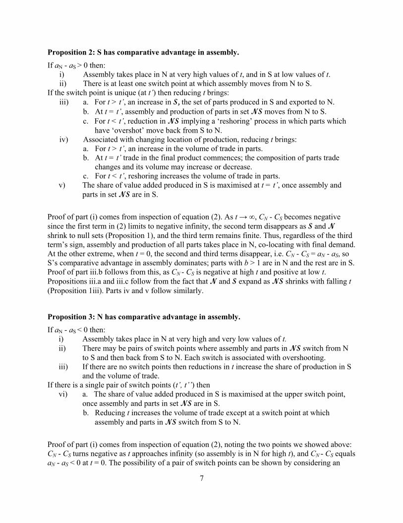
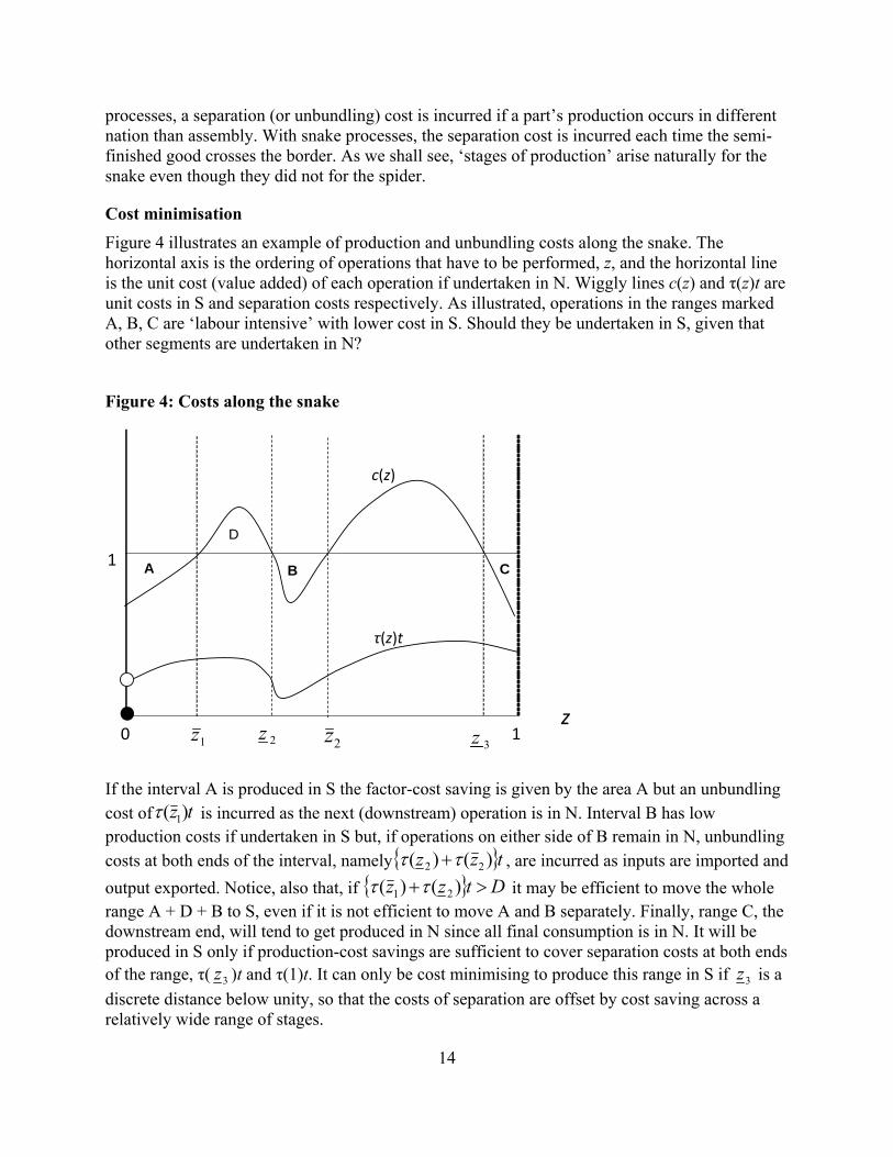
Figure 4 illustrates an example of production and unbundling costs along the snake. The horizontal axis is the ordering of operations that have to be performed, z, and the horizontal line is the unit cost (value added) of each operation if undertaken in N. Wiggly lines c(z) and τ(z)t are unit costs in S and separation costs respectively. As illustrated, operations in the ranges marked A, B, C are ‘labour intensive’ with lower cost in S. Should they be undertaken in S, given that other segments are undertaken in N?

Figure 4: Costs along the snake

If the interval A is produced in S the factor-cost saving is given by the area A but an unbundling cost of tz )( 1 is incurred as the next (downstream) operation is in N. Interval B has low production costs if undertaken in S but, if operations on either side of B remain in N, unbundling costs at both ends of the interval, namely tzz )()( 22 , are incurred as inputs are imported and

output exported. Notice, also that, if Dtzz )()( 21 it may be efficient to move the whole range A + D + B to S, even if it is not efficient to move A and B separately. Finally, range C, the downstream end, will tend to get produced in N since all final consumption is in N. It will be produced in S only if production-cost savings are sufficient to cover separation costs at both ends of the range, τ( 3z )t and τ(1)t. It can only be cost minimising to produce this range in S if 3z is a

discrete distance below unity, so that the costs of separation are offset by cost saving across a relatively wide range of stages.

D

2z  2z  1z  

z1 

3z

A  B  C1

c(z) 

τ(z)t 

0 

15

Equalseparationcosts

We start by concentrating on the implications of variation in production costs, c(z), assuming that the separation cost is ‘t’ wherever it occurs in the production process (i.e. τ(z)=1 for all z). The analysis is facilitated by two concepts: fragments, and stages.

Definition: A fragment is an interval of the production process in which: either c(z) ≥ 1 for all z in the interval and c(z) < 1 at adjacent points: or c(z) < 1 for all z in the interval and c(z) ≥ 1 at adjacent points.

Definition: A stage is an interval of the production process performed in one nation; a ‘pure’ stage is a fragment; a ‘mixed’ stage involves fragments with c(z) ≥ 1 and c(z) < 1. A ‘separation’ occurs at each end of a stage.

Fragments are determined by technology and comparative costs, while stages are endogenous location outcomes and may be the union of adjacent fragments. To simplify exposition we also initially suppose that factor costs in S are either 1+ (for capital-intensive operations) or 1- (for labour-intensive operations). We can then derive the following statement about the relationships between stages and fragments.

Proposition 5: fragments and stages.

i) When t is zero, all fragments are stages. ii) If t > 0, each fragment is contained in a single stage. iii) Fragments that are below some minimum separation size, 2 /m t , will be contained in

the same stage as an adjacent fragment.

Part i) is obvious since in a frictionless world, factor costs are the only consideration and costs are minimised by putting all capital-intensive fragments in N and all labour-intensive fragments in S. Part ii) holds since if costs are reduced by offshoring any parts of a fragment, greater savings are achieved by offshoring all parts in the fragment. Part iii) is true since a fragment that is too small to be worth offshoring on its own will, by default, be bundled with either the preceding or subsequent fragment; these, by definition of a fragment, will have different factor intensity. The definition of m comes from direct calculation; the cost-saving from shipping a labour-intensive fragment from N to S and back (or a capital-intensive sector from S to N and back) is the length of the fragment times , so the shortest fragment for which factor-cost savings cover the separation cost is m = 2t (recall production always starts and ends in N).

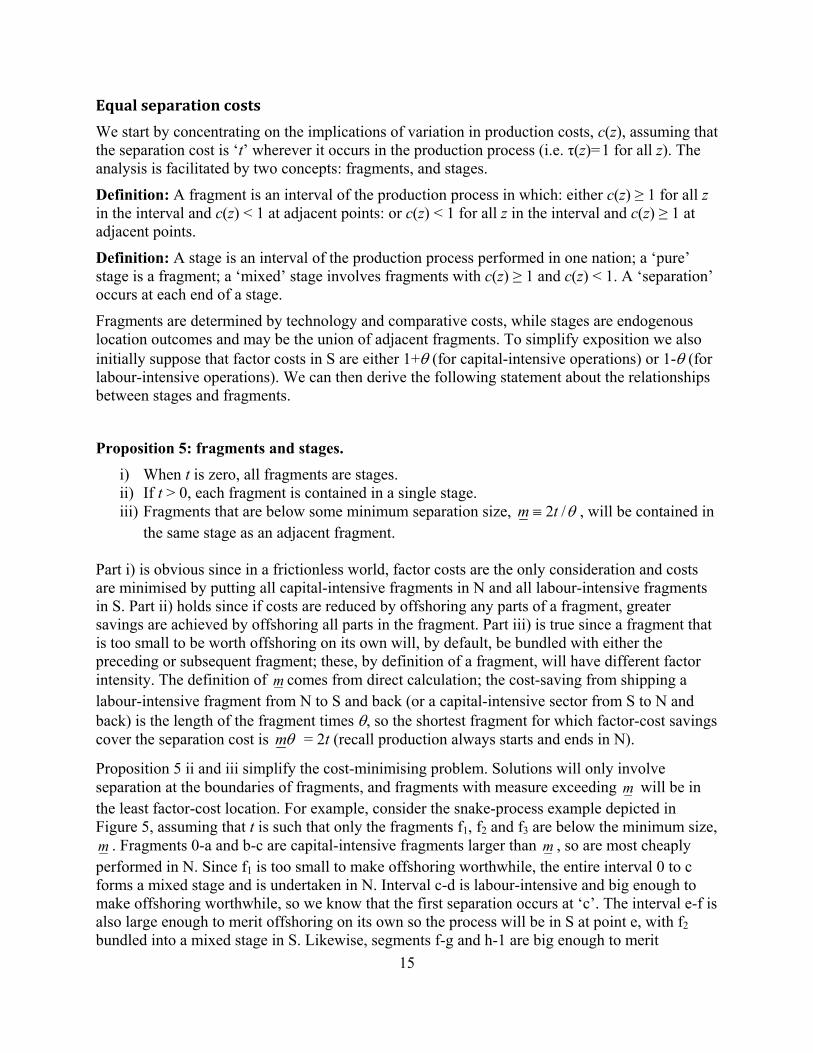
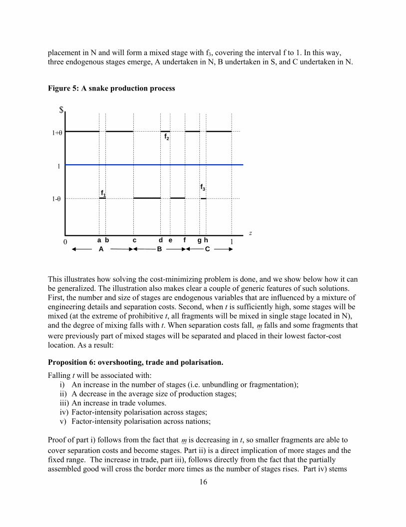
Proposition 5 ii and iii simplify the cost-minimising problem. Solutions will only involve separation at the boundaries of fragments, and fragments with measure exceeding m will be in the least factor-cost location. For example, consider the snake-process example depicted in Figure 5, assuming that t is such that only the fragments f1, f2 and f3 are below the minimum size,m . Fragments 0-a and b-c are capital-intensive fragments larger than m , so are most cheaply performed in N. Since f1 is too small to make offshoring worthwhile, the entire interval 0 to c forms a mixed stage and is undertaken in N. Interval c-d is labour-intensive and big enough to make offshoring worthwhile, so we know that the first separation occurs at ‘c’. The interval e-f is also large enough to merit offshoring on its own so the process will be in S at point e, with f2 bundled into a mixed stage in S. Likewise, segments f-g and h-1 are big enough to merit

16

placement in N and will form a mixed stage with f3, covering the interval f to 1. In this way, three endogenous stages emerge, A undertaken in N, B undertaken in S, and C undertaken in N.

Figure 5: A snake production process

This illustrates how solving the cost-minimizing problem is done, and we show below how it can be generalized. The illustration also makes clear a couple of generic features of such solutions. First, the number and size of stages are endogenous variables that are influenced by a mixture of engineering details and separation costs. Second, when t is sufficiently high, some stages will be mixed (at the extreme of prohibitive t, all fragments will be mixed in single stage located in N), and the degree of mixing falls with t. When separation costs fall, m falls and some fragments that were previously part of mixed stages will be separated and placed in their lowest factor-cost location. As a result:

Proposition 6: overshooting, trade and polarisation.

Falling t will be associated with: i) An increase in the number of stages (i.e. unbundling or fragmentation); ii) A decrease in the average size of production stages; iii) An increase in trade volumes. iv) Factor-intensity polarisation across stages; v) Factor-intensity polarisation across nations;

Proof of part i) follows from the fact that m is decreasing in t, so smaller fragments are able to cover separation costs and become stages. Part ii) is a direct implication of more stages and the fixed range. The increase in trade, part iii), follows directly from the fact that the partially assembled good will cross the border more times as the number of stages rises. Part iv) stems

$

z1

1

0

1-

1+

aA CB

f2

f1

f3

b c f g hd e

17

from the fact that the newly created stages will always involve moving labour-intensive fragments to S or capital-intensive stages to N, and part v) is the country dimension of the reallocation of production in Part iv). Note that 6 i) may involve a capital-intensive fragment moving from S to N,14 in which case we can say that overshooting has taken place and the repatriation of the fragment could be considered ‘reshoring’. It follows that the share of value added in S is not monotonically increasing as t falls.

Generalizations: c(z) and τ(z)

While convenient, the assumption that factor cost differences between N and S are restricted to values c(z) = 1+ θ, c(z) = 1- θ, is not necessary. Suppose that fragment i occupies interval [zi, zi+ζi], and now define m(i) as

ii

i

z

zdzzcabsim

1)()( , (10)

so m(i) is the difference in factor cost of producing fragment i in S rather than in N. It is now the case that fragments with m(i) < m = 2t will be bundled with an adjacent fragment, exactly as in the example above. The difference is simply that m can no longer be interpreted as a ‘length’ of the snake (i.e., a measure of operations z), but instead captures the difference in costs of producing the entire fragment in one country rather than the other. Proposition 6 continues to apply.

The analysis above assumed that separation costs are the same at all points along the snake. This captures the primary effect of reductions in t, which is to enable fragments to move in line with comparative costs. However, if τ(z) varies with z, then changes in t will have an additional, marginal effect on separation points. To see this, consider an alternative example in which S has a comparative advantage in upstream products and N has advantage in downstream products, i.e. c(z) is increasing for all z, with c(0) < 1 and c(1) > 1. There are just two fragments, and the cost minimisation problem is that of choosing the dividing operation z , upstream of which ( zz ˆ ) production takes place in S, while downstream stages zz ˆ take place in N. z is chosen to minimise total costs, denoted )ˆ(zC , and given by:

dztzdzzczCz

z

1

ˆ

ˆ

0)ˆ()()(

. (11)

The first integral is the cost of producing the range z0 in S; tz)ˆ( is the cost of transferring the product to N, and the final integral is the sum of the (unit) cost of producing remaining stages in N. We assume that the functions c(z) and τ(z) are twice differentiable, so first and second derivatives with respect to z are

tzzcz

zUtzzc

z

zU)ˆ(")ˆ(

ˆ

)ˆ(,1)ˆ(')ˆ(

ˆ

)ˆ(2

2

(12)

Suppose initially that the first of these equations, set equal to zero, defines a global cost minimum. If separation costs are uniform, z' = 0, then the dividing operation is where

14 In figure 5, this would correspond to t being low enough that fragment f2 broke out of stage B (produced in S) and became its own stage operating in N.

18

,1ˆ zc as expected. However, if separation costs vary then the dividing point moves in either direction according to whether they are increasing or decreasing with z. For a product adding complexity with each operation, separation costs might increase, z' > 0. The dividing point z

is then where 1ˆ zc , so that some operations with lower costs in S are performed in N. A reduction in t, the common element of separation costs increases the range of operations undertaken in S because, differentiating along the first order condition in (12) ,

0)ˆ()ˆ(

)ˆ('ˆ

tzzc

z

dt

zd

(13)

(the denominator is positive by the second order condition). Conversely, a product such as a natural resource which loses weight as it is processed may have 0' z . This means that more

operations are done in S, 1ˆ zc , since the separation cost saving from shipping a more processed product offsets the higher factor costs of processing in S.

The general analysis of this problem is complex, particularly since second order conditions may fail (see equations (12)). In the working paper version of the paper we illustrate an array of possible outcomes which, once again, may involve overshooting and reshoring.

4. Spiders and snakes; conclusions

It is a commonplace to say that globalization is associated with the fragmentation, unbundling and offshoring of production. But how does this occur given the complexity of actual production processes or value chains? The engineering details of the production process matters and we characterise two extremes as ‘snakes’ and ‘spiders’. Snakes are production processes where a physical entity follows a sequential process with each operation adding value in a predetermined order. Spiders are ‘many limbed’ processes, where parts come together for assembly. In practise the two are combined: spiders might be attached to any part of a snake, and multiple snakes might join into a spider. We conjecture that virtually all production processes can be thought of as combinations of our cases.

Analysis of both spiders and snakes provides insights, some of them similar in the two cases, others different. In both cases location is determined as the outcome of a tension between international differences in production costs and co-location benefits due to unbundling costs. Reductions in international frictions (be they trade costs or communication and coordination costs) facilitate the relocation of production in line with comparative costs, but this relocation is not necessarily continuous or monotonic. Overshooting and reshoring can occur in both the spider and the snake, as parts move against their comparative costs (to save on unbundling costs), and then move back when unbundling costs fall further. In the spider this occurs when assembly relocates, taking a wide range of parts with it some of which move against their comparative costs in order to maintain proximity to the assembler. Further reductions in unbundling costs weaken this co-location force, causing some parts to ‘reshore’. In the snake, reducing separation costs can cause relocation of a range of operations (a stage) which contains both capital and labour intensive fragments. Some of these fragments move against their

19

comparative costs, and further unbundling-cost reductions enable them to move back.15

Both the spider and the snake potentially exhibit coordination failure and hence, if decisions are made independently by separate firms, there may be inefficiently little offshoring as unbundling costs fall. This arises as each firm cannot be sure that, if it were to move, parts to which it is linked (assembly and parts in the spider, adjacent operations in the snake) will move in response. The problem may be particularly acute in the snake where, for example, a capital intensive part may be ‘stuck’ in N because it fails to coordinate with adjacent labour intensive parts. This inefficiency suggests strong incentives to vertically integrate or for firms to take other measures to coordinate actions and achieve the cost minimising outcome.

Other outcomes are quite different for the spider and the snake. In the spider, a part crosses borders at most twice, once as a part and once embodied in final output. The value of trade is bounded by twice the value of final output (value added over all parts and assembly) and does not necessarily increase as trade frictions fall. The value of trade in parts responds in the expected manner for any range of frictions that does not include a switching point. However, over the full range, the relationship between the trade values and trade frictions is neither continuous nor monotonic. Offshoring assembly both creates and destroys trade in parts, reversing the direction of net parts exports in the process. It also may create or destroy trade in final goods – creating it when assembly moves N to S, but destroying it when the switch occurs in the reverse direction.

This is in marked contrast to the spider where falling frictions cause an ever finer slicing of the snake, and a monotonic increase in trade volumes. Stages of production emerge endogenously from the interplay of engineering details (the sequence in which parts must be added), separation costs and comparative cost differences. The ratio of trade to the value of final output is potentially unbounded, depending on the number of separate fragments in the value chain.

A further property of the snake is that falling frictions and consequent relocations cause the factor intensities of activities taken in each country to become increasingly polarised; activities in S become, on average, more labour-intensive, and those in N more capital-intensive.16 Implications for factor prices depend on the full specification of the general equilibrium, beyond the scope of this paper, but the polarization is suggestive of factor price convergence. In contrast, no such general polarisation result holds for the spider.

The tension between factor costs and co-location benefits is, we think, central to analysis of offshoring. The analysis of spiders and snakes undertaken in this paper provides building blocks, and further work needs to extend this to understand technologies that combine snakes and spiders. Empirical work on offshoring needs to recognise the discontinuities and non-monotonic patterns of trade and location that we have uncovered. And policy needs to understand the disruptive potential for abrupt and discontinuous change in the location of related activities.

15 Non-monotonic effects of falling trade frictions is a property shared with many new economic geography models (Fujita et al 1999). In the present context, they arise because, even if trade costs are uniform (as in our examples), production cost savings from relocation vary across parts and operations. 16 Some fragments may move against their comparative costs, but only as part of stages which move in line with the comparative cost of the whole stage.

20

REFERENCES

Ando, M. and F. Kimura (2005). The formation of international production and distribution networks in East Asia. In T. Ito and A. Rose (Eds.), International trade (NBER-East Asia seminar on economics, volume 14), Chicago: University of Chicago Press.

Arndt, S.W. and H. Kierzkowski (Eds.) (2001). Fragmentation: New Production Patterns in the World Economy. Oxford University Press, Oxford.

Baldwin, R. and F. Robert-Nicoud (2010). "Trade-in-goods and trade-in-tasks: An Integrating Framework," NBER Working Papers 15882.

Baldwin, R. and A.J. Venables (2010). ‘Relocating the value chain: offshoring and agglomeration in the global economy’ NBER wp16611

Collins, M. (2010). “Re-shoring–Bringing manufacturing back to American suppliers”. Manufacturing.net, http://www.manufacturing.net/

Costinot, A., J. Vogel and S. Wang (2011). ‘An elementary theory of global supply chains’ NBER working paper 16936.

Davidson, P. (2010). ‘Some manufacturing heads back to USA’, USA Today, August.

Dixit, A. and G. M. Grossman (1982). Trade and Protection with Multi-Stage Production, Review of Economic Studies 49(4), 583-594.

Dixit, A.K. and G. M. Grossman (1982). ‘Trade and Protection with Multistage Production’ Review of Economic Studies, Vol. 49, No. 4, pp. 583-594.

Feenstra, R.C and G.H. Hanson (19906). ‘Globalization, Outsourcing, and Wage Inequality’ American Economic Review, 86, 240-245.

Frigant, V. and Y. Lung (2002). ‘Geographical proximity and supplying relationships in modular production’, International Journal of Urban and Regional Research, 26.4 pp742-55

Fujita, M., P. Krugman, P. and A.J. Venables (1999) The Spatial Economy: Cities, Regions and International Trade. Cambridge, MA: MIT Press.

Fujita, M. and J. Thisse (2006). ‘Globalization and the evolution of the supply chain: who gains and who loses?’ International Economic Review, 47, pp 811-836

Grossman, G. M. and, E. Rossi-Hansberg (2008). Trading Tasks: A Simple Theory of Offshoring, American Economic Review, 98, pp 1978-97.

Harrigan, J. and A.J. Venables (2006). ‘Timeliness and agglomeration’, Journal of Urban Economics, 59, 300-316.

Helpman, E. (1984). A Simple Theory of Trade with Multinational Corporations. Journal of Political Economy 92, 451-471.

Helpman, E. (2006). Trade, FDI and the organization of firms’, Journal of Economic Literature, XLIV, 589-630.

Hummels, D., D. Rapoport and K.-M. Yi, (1998). Vertical Specialization and the Changing Nature of World Trade. Federal Reserve Bank of New York Economic Policy Review 4, 79-99.

21

Hummels, D., J. Ishii, and K-M. Yi (2001). The Nature and Growth of Vertical Specialization in World Trade. Journal of International Economics 54, 75-96.

Hummels, D., J. Ishii, and K-M. Yi (1999). "The nature and growth of vertical specialization in world trade," Staff Reports 72, Federal Reserve Bank of New York.

Johnson, R. C. and G. Noguera (2012). “Accounting for Intermediates: Production Sharing and Trade in Value Added” Journal of International Economics, 86, 224-236.

Jones, R. W. and H. Kierzkowski (2001). A Framework for Fragmentation, in: S.W. Arndt and H. Kierzkowski (Eds), Fragmentation: New Production Patterns in the World Economy, Oxford University Press, Oxford.

Jones, R.W. (2000). Globalization and the Theory of Input Trade, MIT Press, Cambridge.

Kimura, F., Y. Takahashi and K. Hayakawa (2007). "Fragmentation and parts and components trade: Comparison between East Asia and Europe," The North American Journal of Economics and Finance, Elsevier, vol. 18(1), pages 23-40, February.

Klier, T.H. and J. Rubinstein (2009). ‘Imports of Intermediate parts in the auto-industry; a case study’ http://www.upjohninst.org/measurement/klier-rubenstein-final.pdf

Levine, D. (2010). ‘Production chains’, NBER wp 16571

Markusen, J. R. (2002). Multinational Firms and the Theory of International Trade, MIT Press.

Markusen, J.R. and A.J. Venables (2007). ‘Interacting factor endowments and trade costs: a multi-country, multi-good approach to trade theory’, Journal of International Economics, 73, 333-354

Ng, F. and A. Yeats (1999). Production sharing in East Asia; who does what for whom and why. World Bank Policy Research Working Paper 2197, Washington DC.

Rubin, J. and B. Tal (2008). “Will Soaring Transport Costs Reverse Globalization?” StrategEcon, CIBC World Markets Inc. http://research.cibcwm.com

Sako, M. (2005). ‘Governing automotive supplier parks: leveraging the benefits of outsourcing and co-location’, processed, SBS, Oxford.

Sirkin, H., M. Zinser and D. Hohner (2011). “Made in America, Again”, Boston Consulting Group report, August.

Venables, A.J. (1996). ‘Equilibrium locations of vertically linked industries’, International Economic Review, 37, 341-59.

Wu, X. and F. Zhang (2011). “Efficient Supplier or Responsive Supplier? An Analysis of Sourcing Strategies under Competition”, http://ssrn.com/abstract=1871425.

Yi, K-M. (2003). Can Vertical Specialization Explain the Growth of World Trade? Journal of Political Economy 111, 52-102.

22

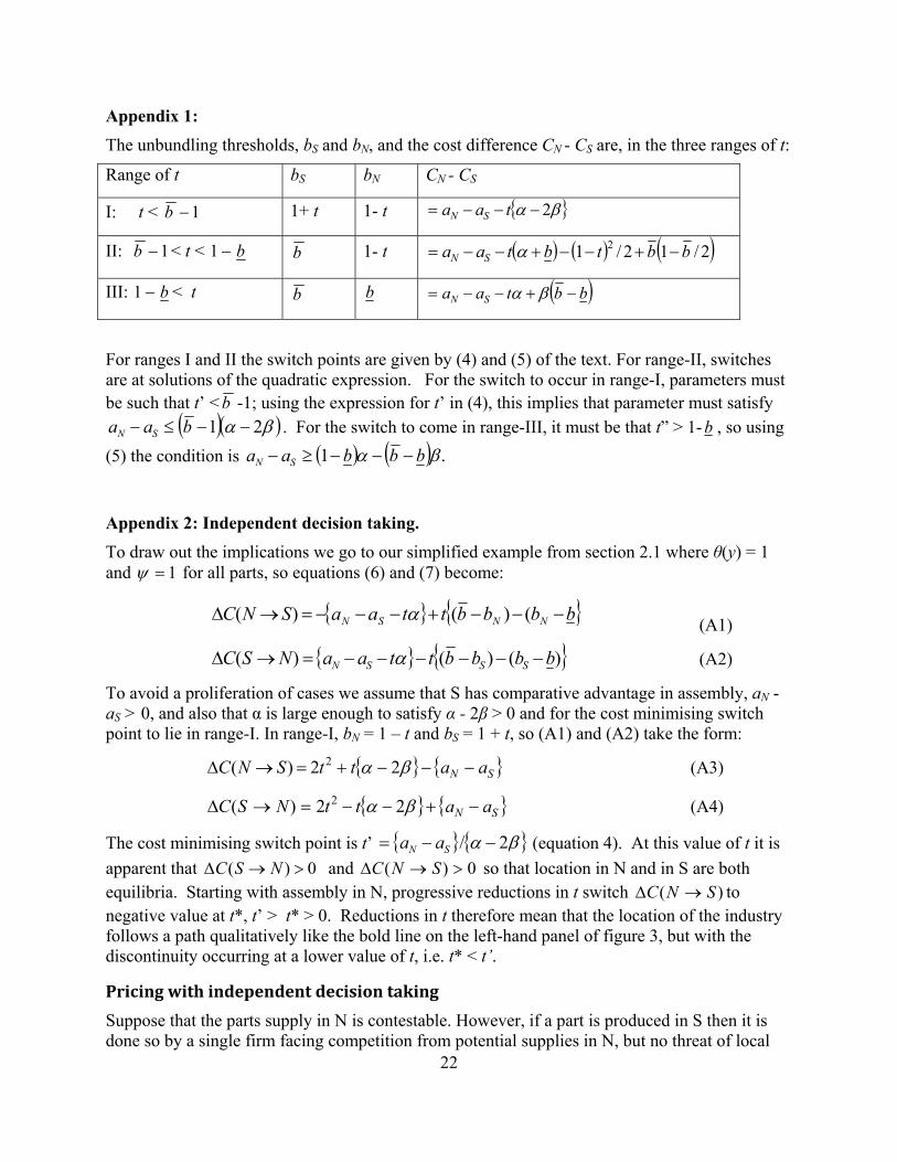
Appendix 1:

The unbundling thresholds, bS and bN, and the cost difference CN - CS are, in the three ranges of t:

Range of t bS bN CN - CS

I: t < 1b 1+ t 1- t 2 taa SN

II: 1b < t < b1 b 1- t 2/12/1 2 bbtbtaa SN

III: b1 < t b b bbtaa SN

For ranges I and II the switch points are given by (4) and (5) of the text. For range-II, switches are at solutions of the quadratic expression. For the switch to occur in range-I, parameters must be such that t’ < b -1; using the expression for t’ in (4), this implies that parameter must satisfy

21 baa SN . For the switch to come in range-III, it must be that t” > 1-b , so using

(5) the condition is .1 bbbaa SN

Appendix 2: Independent decision taking.

To draw out the implications we go to our simplified example from section 2.1 where θ(y) = 1 and 1 for all parts, so equations (6) and (7) become:

bbbbttaaSNC NNSN ()()( (A1)

)()()( bbbbttaaNSC SSSN (A2)

To avoid a proliferation of cases we assume that S has comparative advantage in assembly, aN - aS > 0, and also that α is large enough to satisfy α - 2β > 0 and for the cost minimising switch point to lie in range-I. In range-I, bN = 1 – t and bS = 1 + t, so (A1) and (A2) take the form:

SN aattSNC 22)( 2 (A3)

SN aattNSC 22)( 2 (A4)

The cost minimising switch point is t’ 2/ SN aa (equation 4). At this value of t it is

apparent that 0)( NSC and 0)( SNC so that location in N and in S are both equilibria. Starting with assembly in N, progressive reductions in t switch )( SNC to negative value at t*, t’ > t* > 0. Reductions in t therefore mean that the location of the industry follows a path qualitatively like the bold line on the left-hand panel of figure 3, but with the discontinuity occurring at a lower value of t, i.e. t* < t’.

Pricingwithindependentdecisiontaking

Suppose that the parts supply in N is contestable. However, if a part is produced in S then it is done so by a single firm facing competition from potential supplies in N, but no threat of local

23

competition. We assume that – given the absence of local competition in S – fraction γ of the surplus on a part produced in S is captured by the parts producer. Thus, if the assembler is in N and purchases a part from S, the price paid is )(1 tbtb where the term in square

brackets is the difference between the cost of production in N and the cost of supply from S (i.e. the surplus on the sourcing from S). If the assembler is in S this price becomes btb 1 , where the surplus is cost of supply from N minus cost of production in S. Relocating from N to S, the producer therefore saves t(1-2γ) on each part produced in S (the difference between these two prices). If γ = 0 the assembler would have saved the whole of the unbundling cost t, but part of this surplus is captured by the producer of the part in S. The set of parts supplied from S is unchanged at bbN (set S, given our Nash assumption), so the assembler’s cost savings on parts

produced in S are bbN )21( . The sets S, N and NS are exactly as before, reflecting the

fact that there is no surplus at the margin. The change in assembler’s costs in moving from N to S are now:

( ) ( ) (1 2 )( )S N N NC N S a a t b b b b

This is expression (A1) adjusted for the change in price paid for parts produced in S. A positive value of γ therefore increases the overall change in costs associated with moving assembly from N to S, so makes the move less attractive. The intuition is that moving assembly to S places the assembler in an environment with less competition in the supply of parts. If t is falling through time, a positive value of γ further postpones offshoring, amplifying the inefficiency arising from uncoordinated decision taking.