Embed Size (px)
Citation preview
SPM®
Users Guide Command Reference

2
© 2019 Minitab, LLC. All Rights Reserved.
Minitab®, SPM®, SPM Salford Predictive Modeler ®, Salford Predictive Modeler®, Random Forests®, CART®, TreeNet®, MARS®, RuleLearner®, and the Minitab logo are registered trademarks of Minitab, LLC. in the United States and other countries. Additional trademarks of Minitab, LLC. can be found at www.minitab.com. All other marks referenced remain the property of their respective owners.
Salford Predictive Modeler® Command Reference
3
Getting Started
This guide provides a command language reference and syntax.
SPM® has two alternative modes of control in, command-line and batch. For users running SPM in these modes, knowing the proper command syntax is a must. This guide contains a detailed description of the command syntax and options available.
ANOMALY
Purpose
ANOMALY performs anomaly (outlier) detection. For each variable in the KEEP list (by default, all
variables), the univariate distribution is determined. The percentile of each data point is determined and mapped to a score in the range [-.5, .5]. The product of scores for each variable is taken to determine the anomaly score for the entire data record. The command syntax is: ANOMALY [ GO, SAVE="filename", REPORT=<yes|no>, MODEL=<yes|no>, MISSING=<HIGH|LOW|OMIT> ]
SAVE will save your data, along with the anomaly score, the record's case weight and the data sample
(learn/test/holdout) to an output dataset. REPORT will describe the distribution of the anomaly score,
separately for learn, test and holdout samples. MODEL will build regression models of the anomaly score,
using CART®, TreeNet®, MARS®, Random Forests®, GPS and linear regression in an effort to interpret why records might be outliers. MISSING controls whether missing values are treated as "low" (extremely
negative), "high" (extremely positive) or are omitted from computations of anomaly scores. The default is MISSING=OMIT.
By default the ANOMALY command considers all the variables in your dataset, but will be restricted to your
KEEP list if you have one.
AUXILIARY
Purpose
CART only. The AUXILIARY command specifies variables (either in the model or not) for which node-specific statistics are to be computed in a CART tree. For continuous variables, statistics such as N, mean, min, max, sum, SD and percent missing may be computed. Which statistics are actually computed is specified with the DESCRIPTIVE command. For discrete/categorical variables, frequency tables are produced showing the most prevalent seven categories.
The command syntax is:
AUXILIARY <variable>, <variable>, ...
Variable groups may be used in the AUXILIARY command similarly to variable names.
Salford Predictive Modeler® Command Reference
4
AUTOMATE
Purpose
The AUTOMATE command generates a group of models by varying one or more features or control parameters of the model. SPM offers over 80 different automated modeling options, most of which are available for multiple analysis engines. Each of the automate options is described separately below.
AUTOMATE ATOM
CART and RandomForests only. You can specify your own ATOM values with the VALUES option, otherwise a selection of default atoms will be used (for CART: 2, 5, 10, 25, 50, 100, 200, 500, or for Random Forests: 2, 5, 10, 20, 30).
REPEAT will repeat the experiment with different random seeds.
AUTOMATE ATOM [ VALUES=<n1>,<n2>,..., REPEAT=<N> ]
REPEAT will repeat the experiment with different random seeds.
AUTOMATE CVFOLDS
CART, TreeNet and MARS only. AUTOMATE CVFOLDS varies the number of "folds" used in cross validation. The defaults are 5, 10, 20 and 50 CV folds. REPEAT will repeat the experiment with different random seeds.
AUTOMATE CVFOLDS [ VALUES=<n1>,<n2>,..., REPEAT=<N> ]
REPEAT will repeat the experiment with different random seeds.
AUTOMATE DEPTH
CART only. Generates one unconstrained and seven depth-limited (4, 8, 12, 16, 20, 24, 30) models. You may provide a list of depths to which you wish to constrain the tree, in which case 0 indicates an unconstrained model:
AUTOMATE DEPTH [ VALUES=<n1>,<n2>,..., REPEAT=<N> ]
REPEAT will repeat the experiment with different random seeds.

Salford Predictive Modeler® Command Reference
5
AUTOMATE FLIP
AUTOMATE FLIP generates two models by reversing 50% learn / test samples. If the REPEAT=N option is USE d, a total of 2*N models will be built, with the learn/test partition being randomly redrawn between each pair. REPEAT will repeat the experiment with different random seeds.
AUTOMATE FLIP [ REPEAT=<n> ]
AUTOMATE LEARNRATE
TreeNet only. AUTOMATE LEARNRATE generates three models using, by default, learn rate of 0.001, 0.01 and 0.1, e.g., but you can specify your own values with:
AUTOMATE LEARNRATE [ VALUES=<n1>,<n2>,..., REPEAT=<N> ]
REPEAT will repeat the experiment with different random seeds.
AUTOMATE MISSING_PENALTY
CART only. AUTOMATE MISSING_PENALTY generates five models: main effects, main effects with missing value indicators (MVI), MVIs only, main effects with missing values penalized, main effects and MVIs with missing values penalized. If your predictors have no missing data, AUTOMATE MISSING_PENALTY is not informative.
AUTOMATE MINCHILD
CART and TreeNet only. AUTOMATE MINCHILD varies the MINCHILD setting (the minimum allowable size of a terminal node). By default, it will build eight models using settings of 1, 2, 5, 10, 25, 50, 100 and 200 for CART and seven models using settings of 3, 5, 10, 25, 50, 100, 200 for TreeNet. You can specify your own values with:
AUTOMATE MINCHILD [ VALUES=<n1>,<n2>,..., REPEAT=<N> ]
REPEAT will repeat the experiment with different random seeds.
AUTOMATE NEST
Do we nest (combine) automate specifications?
AUTOMATE NEST [ = YES | NO ]
Salford Predictive Modeler® Command Reference
6
AUTOMATE NODES
CART and TreeNet only. AUTOMATE NODES varies the allowable number of nodes permitted in the tree. By default it will build four models. For TreeNet models, the default is that trees are limited to 2, 4, 6 and 9 terminal nodes. For CART models, the default is that trees are limited to 4, 8, 16 and 32 terminal nodes. You may specify a custom set of values with the VALUES option, e.g.,
AUTOMATE NODES [ VALUES=<n1>,<n2>,..., REPEAT=<N> ]
REPEAT will repeat the experiment with different random seeds.
AUTOMATE POWER
CART only. AUTOMATE POWER varies CART's "power end cut" parameter. The default values are 1, 2, 3, 5, 10, but you can specify your own values, e.g.,
AUTOMATE POWER [ VALUES=<n1>,<n2>,..., REPEAT=<N> ]
REPEAT will repeat the experiment with different random seeds.
AUTOMATE ONEOFF
AUTOMATE ONEOFF attempts to model the target as a function of one predictor at a time. Note that for CART classification models, the class probability splitting rule is used. AUTOMATE ONEOFF will generate as many models as there are predictors. AUTOMATE ONEOFF is the complement of AUTOMATE LOVO.
AUTOMATE ONEOFF
AUTOMATE LOVO
AUTOMATE LOVO repeat the model leaving one predictor out of the model each time. Note that for CART classification models, the class probability splitting rule is used. AUTOMATE LOVO is the compliment of ONEOFF.
AUTOMATE LOVO
Salford Predictive Modeler® Command Reference
7
AUTOMATE PRIOR
CART only. AUTOMATE PRIOR varies CART only. Vary the priors for the specified class from 0.005 to 0.995 in steps of equal and/or varying size. If you wish to specify a particular set of values, use the START, END and INCREMENT options, e.g.
AUTOMATE PRIOR=<target_class> [, BINARY=<LINEAR|RATIO|BLEND>, SHARE=<yes|no> ]
If you wish to specify a particular set of values, use the START, END and INCREMENT options, e.g.
AUTOMATE PRIOR=3 START=.5 (will infer END and INCREMENT settings) AUTOMATE PRIOR="Male" START=.45, END=.75, INCREMENT=.01
For a binary target, you can use a default selection of response class priors that are LINEARly distributed from 0 to 1, or indicate that the RATIO of response to nonresponse priors is linearly distributed, or use a BLENDing of the two methods. When the BINARY option is used (with either LINEAR, RATIO or BLEND), it supersedes the START, END and INCREMENT options.
For binary targets, the priors that are specified (either explicitly, or through the LINEAR, RATIO or BLEND options) are further optimized by the learn sample share of the <target_class>. To disable this optimization, use the option SHARE=NO. The default is SHARE=YES.
AUTOMATE PRIOR is an essential component in SPM's HOTSPOT detection in which we search for individual nodes in CART trees that show unusually high LIFT or concentration of the target class. For successful hotspot detection you need to explore low priors values on the class you are interested in and you need not be concerned if many of the trees developed by the Automate are null or show overall poor performance. Only the lift in specific nodes matters in hotspot detection.
AUTOMATE RULES
CART only. AUTOMATE RULES generates a model for each splitting rule (six for classification, two for regression). Note that for the TWOING model, POWER is set to 1.0 to help ensure it differs from the GINI model.
AUTOMATE RULES
AUTOMATE SHAVING RFE (Recursive Feature Elimination)
CART, MARS, TreeNet, and Random Forests only. Shave (remove) predictors from the model, cycling until the specified number of steps (STEPS=) have been completed or until there are no predictors left. SPM can shave from the TOP (most important are shaved first) or BOTTOM (least important variables shaved first). TOP and BOTTOM can shave N predictors at a time (SHAVING=N).
AUTOMATE SHAVING [=<n>,] TOP|BOTTOM [, STEPS=<n>, CORE=<varlist>, PERCENT=<x>]
AUTOMATE SHAVING ERROR [, STEPS=<n>, CORE=<varlist>,
CRITERION=<MSE|MAD> ]
Salford Predictive Modeler® Command Reference
8
CORE predictors, if any, are not shaved until all non-CORE predictors have been shaved. The CORE option, if used, must be the final option on the AUTOMATE command. The defaults are to shave one predictor at a time from the bottom until the model degenerates to nothing.
ERROR determines which predictor to shave next by leaving one variable out (LOVO) at a time and then rerunning the model to assess which predictor is least or most important. SHAVING ERROR can require a very large number of models to be run; with K variables and requesting K steps, K*(K+1)/2 models will be needed. For K=20 this is 110 models. For K=50 this is 1,275.
CRITERION defines the performance criterion (independent of the loss function) and applies to TreeNet regression models only at this time.
PERCENT will shave a percentage of the remaining predictors at each step. If SHAVING=N and PERCENT=X are issued, PERCENT will take precedence. PERCENT=X should be a value between 0 and 100 noninclusive. PERCENT is ignored for AUTOMATE SHAVING ERROR. For example, to shave 20% of the predictors at each step, use
AUTOMATE SHAVING, PERCENT=20
E.g., if there are 25 predictors in total, 5 (of 25) would be shaved at the first step, then 4 (of 20 remaining) would be shaved at the second step, and so forth.
Builds a set of models with systematically varying target variables, and optionally imputes missing values and missing value indicators that can be saved to a new data set.
Build a set of models systematically rotating through a list of target variables.
To build models for a set of targets on a common set of predictors use the syntax:
KEEP <predictor1>, <predictor2,...>, ...
AUTOMATE TARGET=<target1>, <target2>, ...
AUTOMATE TARGET
AUTOMATE TARGET: Each target variable will be modeled using the variables on the KEEP command as predictors. You may list all targets and predictors together on the KEEP statement as any variable in the TARGET list will not appear as a predictor in ANY model. The TARGET and predictor groups will be kept distinct by the AUTOMATE.
To build a set of models for mutual prediction of any one variable on the KEEP list by all other variables on the KEEP list issue:
AUTOMATE TARGET
This will ignore any existing target variable and use the current KEEP list as the set of variables through which to rotate.
Command options (following a forward slash (/)
AUTOMATE TARGET [ / MP=<yes|no>, MT=<yes|no>,
MISSINGONLY=<yes|no>, SAVE=<"filename"> ]
Salford Predictive Modeler® Command Reference
9
MP governs whether MVIs are used as predictors. The default is MP=YES.
MT governs whether MVIs are used as targets. The default is MT=YES.
MISSINGONLY governs whether MVIs are saved to the output dataset. The default is MISSINGONLY=NO. MISSINGONLY=YES is useful when using AUTOMATE TARGET with an end goal of imputation of missing values.
SAVE saves the predicted values to a new dataset. Since AUTOMATE TARGET is often used to develop imputation models for the target variables, the SAVEd dataset will include imputation columns.
For Random Forests models only: if proximity matrices are enabled, the pooled proximity matrix (pooled, or summed, across all RF models) can be saved to a dataset with the PROXIMITY option:
AUTOMATE TARGET ... PROXIMITY=<"filename"> ...
Furthermore, clustering of the pooled proximity matrix can be saved to a dataset with the CLUSTER option:
AUTOMATE TARGET ... CLUSTER=<"filename"> ...
The clustering options are specified on the RF command, e.g.,
RF CLUSTERS=5,12, LINKAGE=COMPLETE,CENTROID
AUTOMATE CVREPEATED
CART, TreeNet, MARS cross validation models only. AUTOMATE CVREPEATED will repeat the cross validation process N times with different random seeds each time. The SAVE option saves out-of-bag predictions for CART regression models only:
AUTOMATE CVREPEATED=<n> [ SAVE=<"filename"> ]
AUTOMATE KEEP
AUTOMATE KEEP will repeat the model NR times, selecting a subset of NK predictors from the KEEP list each time. The CORE option defines a group of predictors (from the main KEEP list) that are included in each of the models of the Automate. The CORE option, if used, must be the final option on the AUTOMATE command. If not explicitly specified, the default number of predictors included in each model (NK) is the square root of the number of predictors in the full KEEP list. The default number of repetitions (NR) is 10.
AUTOMATE KEEP=<NK,NR> [ CORE=<predictor>,<predictor>,...]
Alternatively, you can request all single, double, triple, or quadruple predictor combinations with this syntax:
AUTOMATE KEEP [ SINGLES, DOUBLES, TRIPLES, QUADS ]
Any or all of the SINGLES|DOUBLES|TRIPLES|QUADS option may be given, in which case no <NK,NR> option is needed.

Salford Predictive Modeler® Command Reference
10
AUTOMATE TARGETSHUFFLE
CART, TreeNet, MARS models only. AUTOMATE TARGETSHUFFLE will perform Monte Carlo shuffling (permutation) of the target. Essentially the values of the target are moved from their original rows to other rows at random, otherwise leaving the target and the predictors intact. The permutation is run several times to explore the distribution of performance results due to the shuffling of the data. Typical values for the number of repetitions would be 10, 30, 100, with larger numbers allowing more accurate assessments. REPEAT will repeat the experiment with different random seeds.
Essentially the values of the target are moved from their original rows to other rows at random, otherwise leaving the target and the predictors intact. The permutation is run several times to explore the distribution of performance results due to the shuffling of the data. Typical values for the number of repetitions would be 10, 30, 100, with larger numbers allowing more accurate assessments.
AUTOMATE TARGETSHUFFLE [ =<n>, ST=<YES|NO>, BASELINE=<YES|NO>, REPEAT=<N> ]
If the model has true predictive power the performance of the unperturbed data model should lie outside the range of performances from the permuted data models. The classic output produces a table comparing these results.
The first model built is on unperturbed data. Successive models have the target shuffled to break the correlation between target and explanatory variables.
For CART models AUTOMATE TARGETSHUFFLE may be combined with AUTOMATE RULES.
The ST option controls whether the test sample (if there is one) is shuffled, the default is NO.
The BASELINE option controls whether an unperturbed model is built first. If BASELINE=YES (which is the default), there will be a total of N+1 models built, otherwise there will be N models built.
REPEAT will repeat the experiment with different random seeds.
AUTOMATE QUIET
AUTOMATE QUIET controls how much output is presented as the models are built. Typically you will want only a small amount of summary output, so AUTOMATE QUIET=YES or AUTOMATE QUIET=AUTO are the best choices. Some results that would be produced for a single model are not produced for certain automates. You can disable this output for all automates with AUTOMATE QUIET=YES, produce it with AUTOMATE QUIET=NO or allow the program to decide what output is presented with AUTOMATE QUIET=AUTO.
AUTOMATE QUIET [ = YES | NO | AUTO]

Salford Predictive Modeler® Command Reference
11
AUTOMATE ENABLETIMING
AUTOMATE ENABLETIMING enables simple console timing reports as models are built in an automate.
AUTOMATE ENABLETIMING [=YES|NO|AUTO]
AUTOMATE VARIMP
AUTOMATE VARIMP indicates whether a variable importance matrix report should be produced when possible for CART or TN automates. By default, it is produced for AUTOMATE TARGET only, but it is possible to produce this report for most other CART or TN automates. AUTOMATE VARIMP [ = YES | NO ]
AUTOMATE VARIMPFILE
AUTOMATE VARIMPFILE indicates whether to save the variable importance matrix to a text (comma-separated) file for CART and TreeNet automates only.
AUTOMATE VARIMPFILE = < "filename" >
AUTOMATE LEARN_CURVE
AUTOMATE LEARN_CURVE will result in a series of N models in which the learn sample is reduced randomly N times to examine the effect of learn sample size on error rate. If not specified, N defaults to 10. It is supported for CART®, TreeNet®, MARS®, RandomForests®, LOGIT, REGRESS and GPS models that do not use cross validation. The full learn sample will be used in the first model, followed by models that exclude 1/N, then 2/N, etc. of the learn sample.
Previously, AUTOMATE LEARN_CURVE would build a series of 5 models using all, 3/4, 1/2, 1/4 and 1/8 of the complete learn sample. This mode can be specified with the command AUTOMATE LEARN_CURVE=LEGACY.
AUTOMATE LEARN_CURVE=<N>
AUTOMATE MODELS
AUTOMATE MODELS runs all possible model types, according to how the application is licensed, e.g., CART®, TreeNet®, RandomForests®, MARS®, GPS, Logistic Regression, and Regression. It is supported for regression and binary classification only. Cross validation is not supported for AUTOMATE MODELS, which will default to a random 20% test sample unless something else is explicitly specified.
AUTOMATE MODELS
Salford Predictive Modeler® Command Reference
12
NOTE: GPS, Logit, and Regression apply list-wise deletion of records with missing values in any predictor whereas the other methods do not, meaning that models may be based in different subsets of the data and may not be comparable.
AUTOMATE DRAW
AUTOMATE DRAW builds a series of models in which the learn sample is repeatedly drawn (without replacement) from the "main" learn sample. The test sample is not altered. The proportion to be drawn (in the range 0.01 to 0.99) and number of repetitions may be user specified:
AUTOMATE DRAW [ =<proportion> [, REPEAT=<n> ]]
The default is:
AUTOMATE DRAW=0.50 REPEAT=10
which repeats the model 10 times, each with a random 50% draw of the available learning data.
AUTOMATE PARTITION
AUTOMATE PARTITION builds a series of models in which the learn, test and holdout samples are repeatedly drawn from the data. The data are initially pooled into a single sample for which descriptive statistics are provided. Then, for each model, the data are partitioned randomly into learn, test and holdout samples using the proportions specified on the AUTOMATE PARTITION command:
AUTOMATE PARTITION LEARN=<lprop>, TEST=<tprop>, HOLDOUT=<hprop>,
REPEAT=<nreps>, VARYHOLDOUT=<YES|NO>, MATCHSINGLE=<YES|NO>
The proportions should be in the range 0 to 1 and number of repetitions should be 1 or greater. The default is:
AUTOMATE PARTITION LEARN=0.50 TEST=0.50 HOLDOUT=0.0 REPEAT=10
which repeats the model 10 times, splitting the available data evenly between learn and test samples (with no holdout sample). For example, to produce 30 models using 60% of the data for learn, 30% for test and 10% for holdout each time, use:
AUTOMATE PARTITION LEARN=0.60 TEST=0.30 HOLDOUT=0.10 REPEAT=30
To produce 20 models using 40% of the data for learn, 30% for test and 30% for holdout each time, ensuring that the same holdout sample is used for all models (learn and test samples vary from model to model), use:
AUTOMATE PARTITION LEARN=0.40, TEST=0.30, HOLDOUT=0.30,
REPEAT=20, VARYHOLDOUT=NO
MATCHSINGLE=YES will use, for the first model in the Automate, the same learn/test/holdout partitioning that would have been used in a standalone (non-Automate) model, making comparison of results with the

Salford Predictive Modeler® Command Reference
13
standalone model easy. MATCHSINGLE=NO will use a different random partitioning, and is provided to recreate results produced by previous versions of SPM. The default is MATCHSINGLE=YES.
The default is:
AUTOMATE PARTITION LEARN=0.5, TEST=0.5, REPEAT=10, VARYHOLDOUT=YES,
MATCHSINGLE=YES
AUTOMATE BOOTSTRAP
AUTOMATE BOOTSTRAP builds a series of models, all sharing a common set of options with the exception that each is built from a bootstrapped version of the learn sample. Bootstrapping is done with replacement, meaning that some records in the learn sample may appear more than once in the bootstrapped sample while other records may not appear at all. The options are:
AUTOMATE BOOTSTRAP TEST=OOB|NONE|CROSS,
REPEAT=<n>, REFERENCE=<YES|NO>, RSPLIT=<n>,
LDRAW=<n>, SAVE="filename.ext",
VARIMP=<YES|NO>, NPREPS=<n>,
PROX="filename.ext", NODE="filename.ext",
TREESIZE=<FIXED|POISSON>, EVAL=<OPTIMAL|MAXIMAL>
REFERENCE an initial reference model that does not employ any bootstrap sampling or manipulation of the learn or test samples, can be built. The reference model is essentially what you would build if, instead of using AUTOMATE BOOTSTRAP, you built a single model. The default is REFERENCE=NO, in which no reference model is built.
TEST the TEST option specifies how a test sample, if any, is to be defined for each model. OOB uses out-of-bag learn sample records for the cycles other than the reference model. NONE does not use any test sample for the cycles (i.e., no pruning), other than for the reference model. CROSS use cross validation for all cycles other than the reference model. The default is NONE.
REPEAT specifies the number of cycles, or models, that are to be built, in addition to a possible reference model. The default is 10.
LDRAW specifies a target size of the bootstrapped learn sample. Normally, the bootstrapped learn sample has as many records as the original learn sample. If you wish to force the bootstrapped learn sample to have, say, 20000 records instead, use LDRAW=20000.
SAVE saves In-BAG/OOB indicators and scores, for CART and TN models only, to a dataset.
RSPLIT for CART models, if you wish to consider splitting each node on just a random subset of the available predictors. For instance, if you wish to consider only 4 predictors at each node, independently sampled for each node, use RSPLIT=4. This is similar to the Random Forests algorithm.
VARIMP produces RandomForests-type variable importance measures by randomly permuting in-bag and out-of-bag data to evaluate the impact that a predictor has on each model. Note that this option is potentially very memory intensive and time consuming.
NPREPS specifies the number of random perturbations to be done for each model, when VARIMP=YES. The default is 1.
PROX="filename" produces a proximity matrix based on OOB data for CART models only. The main diagonal is a count of times the record was drawn "out of bag".

Salford Predictive Modeler® Command Reference
14
NODE="filename" stores terminal nodes (that are used to determine the proximity matrix) for CART models only. Negative values represent in-bag, positive values out-of-bag.
TREESIZE=POISSON causes tree sizes to be random based on the Poisson distribution using the LIMIT NODES setting as the mean. This affects CART models only.
EVAL for CART models that use a testing method (cross validation or some form of a test sample), the default is to present performance measures in the Automate summary report for the optimal pruning of each tree. You can instead request that the maximal tree be presented instead with EVAL=MAXIMAL. The default is EVAL=OPTIMAL. This option only affects the classic (text) presentation of results, not the graphic presentation.
For example:
AUTOMATE BOOTSTRAP TEST=NONE REPEAT=100 RSPLIT=4
will repeat the model 100 times, without using any test data, and randomly selecting 4 potential splitters at each node.
AUTOMATE SUBSAMPLE
CART only. AUTOMATE SUBSAMPLE varies the sample size that is used at each node to determine competitor and surrogate splits. The default settings result in an initial model using no subsampling followed by five models using subsampling of 100, 250, 500, 1000 and 5000:
AUTOMATE SUBSAMPLE [ VALUES=<n1,n2,...>, REPEAT=<N> ]
You may list a set of values with the VALUES option as well as a repetition factor (each subsampling size is repeated N times with a different random seed each time), e.g.:
AUTOMATE SUBSAMPLE VALUES=1000,2000,5000,10000,20000,0
AUTOMATE SUBSAMPLE VALUES=1000,2000 REPEAT=20
In the above example, note that 0 denotes a model for which subsampling is not used. REPEAT will repeat the experiment with different random seeds.
AUTOMATE INTER
MARS only. AUTOMATE INTER varies the number of interactions used in MARS models:
AUTOMATE INTER [ VALUES=<n1,n2,...>, REPEAT=<N> ]
The default values are 1, 2 and 3 interactions. REPEAT will repeat the experiment with different random seeds. REPEAT will repeat the experiment with different random seeds.

Salford Predictive Modeler® Command Reference
15
AUTOMATE BASIS
MARS only. AUTOMATE BASIS varies the number of basis functions in MARS models:
AUTOMATE BASIS [ VALUES=<n1,n2,...>, REPEAT=<N> ]
The default is to build four models using 5, 10, 20 and 30 basis functions. REPEAT will repeat the experiment with different random seeds. REPEAT will repeat the experiment with different random seeds.
AUTOMATE MINSPAN
MARS only. AUTOMATE MINSPAN varies the minimum span in MARS models:
AUTOMATE MINSPAN[ VALUES=<n1,n2,...>, REPEAT=<N> ]
The default is to build four models using minimum span values of 0, 5, 10, and 25. REPEAT will repeat the experiment with different random seeds. REPEAT will repeat the experiment with different random seeds.
AUTOMATE SPEED
MARS only. AUTOMATE SPEED varies the MARS speed parameter through all meaningful values. REPEAT will repeat the experiment with different random seeds.
AUTOMATE SPEED [ REPEAT=<N> ]
AUTOMATE PENALTY=MARS
MARS only. AUTOMATE PENALTY=MARS varies the MARS penalty
AUTOMATE PENALTY=MARS [VALUES=<n1,n2,...>, REPEAT=<N>]
Default values are 0.0, .02, .04, .06, .08, and .10. REPEAT will repeat the experiment with different random seeds.
AUTOMATE PENALTY=HLC
CART and MARS only. AUTOMATE PENALTY=HLC varies the exponent term of the HLC penalty, which penalizes a predictor's improvement based on the number of classes found for the splitter within a partition of data, in the range 0 to 2:
AUTOMATE PENALTY=HLC [VALUES=<n1,n2,...>, REPEAT=<N>]
Defaults values are 0, 1.0, and 1.5. REPEAT will repeat the experiment with different random seeds.
Salford Predictive Modeler® Command Reference
16
AUTOMATE PENALTY=MISSING
CART and MARS only. AUTOMATE PENALTY=MISSING varies the exponent term of the MISSING penalty, which penalizes a predictor's improvement based on the proportion missing for the splitter within a partition of data, in the range 0 to 5:
AUTOMATE PENALTY=MARS [VALUES=<n1,n2,...>, REPEAT=<N>]
REPEAT will repeat the experiment with different random seeds.
AUTOMATE STEPWISE
CART, MARS, TreeNet, Random Forests, Logit, GPS, Regress models only only. AUTOMATE STEPWISE builds a series of model by forward-stepwise selection of predictors. The model can be initially empty, or can begin with a set of "core" predictors. The command syntax is:
AUTOMATE STEPWISE [ STEPS=<n>, CORE=<var1>,<var2>, CRITERION=<MSE|MAD>,...]
The CORE option, if used, must be the final option on the AUTOMATE command.
The STEPS option, if used, sets a limit on the number of steps taken. It must be two or greater. If not specified the stepping continues as far as possible.
CRITERION defines the performance criterion (independent of the loss function) and applies to TreeNet regression models only at this time.
For Example:
AUTOMATE STEPWISE
AUTOMATE STEPWISE, STEPS=10
AUTOMATE STEPWISE, STEPS=8, CORE=GENDER,AGE,INCOME

Salford Predictive Modeler® Command Reference
17
AUTOMATE XONY
AUTOMATE XONY builds a series of models in which each predictor serves as the target, and the target serves as the sole predictor:
AUTOMATE XONY
AUTOMATE CVBIN
CART, TreeNet, and MARS only. AUTOMATE CVBIN generates a series of cross-validation models, with binning defined by the several discrete variables listed after the CVBIN option:
AUTOMATE CVBIN=<variable>,<variable>,...
AUTOMATE STRATA
AUTOMATE STRATA generates a series of models for each level of the STRATA variable, provided there is enough variation in the target and predictors to allow a model.
AUTOMATE STRATA [ POOLED=<YES|NO>, TOPMOST=<N>, BOTTOMMOST=<N>, MINLEARN=<N>, MINTEST=<N>, MISSING=<YES|NO>, PMINLEARN=<N>, PMINTEST=<N>, REQUIRE [...], PREQUIRE [...], MAXSTRATA=<N> ]AUTOMATE STRATA [
POOLED=<YES|NO>, TOPMOST=<N>, BOTTOMMOST=<N>, MINLEARN=<N>, MINTEST=<N>, MISSING=<YES|NO>, PMINLEARN=<N>, PMINTEST=<N>, REQUIRE [...], PREQUIRE [...], MAXSTRATA=<N> ]
The POOLED option controls whether an "overall" model, pooling all the strata, is also built. TOPMOST=N controls whether only the most populous N strata are modeled, otherwise all strata are modeled. Similarly with BOTTOMMOST. When TOPMOST and BOTTOMMOST are both issued, TOPMOST will take precedence.
When TOPMOST and BOTTOMMOST are both issued, TOPMOST will take precedence.
MINLEARN=N dictates that a stratum must have at least N records in its learn sample in order to be modeled. Similarly for MINTEST, for the test sample. PMINLEARN and PMINTEST set minimum record counts for the learn and test partitions of individual strata, controlling whether a stratum is included in the pooled model (if a pooled model is estimated).
The REQUIRE and PREQUIRE clauses define more stringent requirements in order for individual (REQUIRE) or pooled (PREQUIRE) strata to be modeled. Options for REQUIRE and PREQUIRE are: N, SUMWEIGHT, NMISS, SUM, MINIMUM, MAXIMUM, MEAN, PROPORTION and PMISS.
The POOLED option controls whether an "overall" model, pooling all the strata, is also built. TOPMOST=N controls whether only the most populous N strata are modeled, otherwise all strata are modeled. Similarly with BOTTOMMOST.
For example:
AUTOMATE STRATA ... REQUIRE MEAN(AGE)>50,
Salford Predictive Modeler® Command Reference
18
REQUIRE PROP("MALE")>.45
N and SUMWEIGHT can either stand alone, in which case they refer to the count of records
in a stratum, or they can be paired with a numeric variable or a target class. If a
numeric variable is specified, it must be in parens. If a target class is specified,
it must be in curly brackets {} and, if the class is a character string, it must be in
quotes. For example:
AUTOMATE STRATA ... REQUIRE N >= 100
AUTOMATE STRATA ... REQUIRE SUMWEIGHT(X) >= 500.0
AUTOMATE STRATA ... PREQUIRE N{"Male"} < 1000
AUTOMATE STRATA ... REQUIRE N{0} > 20
PROPORTION requires a target class to be specified in curly brackets, and quoted if the
target class is a character string). For example
AUTOMATE STRATA ... REQUIRE PROPORTION{"Male"} > 0.1
AUTOMATE STRATA ... PREQUIRE PROPORTION{1} > 0.05
Conditions based on simple continuous statistics allow for further control of which
strata are modeled: NMISS (count of missing values), SUM, MINIMUM, MAXIMUM, MEAN, PMISS
(proportion missing). Each requires a numeric variable to be specified. For example:
AUTOMATE STRATA ... REQUIRE MEAN(INCOME) > 30000.0
AUTOMATE STRATA ... REQUIRE MAXIMUM(AGE) <= 64.0
AUTOMATE STRATA ... PREQUIRE SUM(SALES_DOLLARS) > 10000000.0
AUTOMATE STRATA ... PREQUIRE PMISS(X) < 0.2
Note: by default, a maximum of 200 strata are supported. If you wish to have more strata
than that, use the MAXSTRATA option, e.g.,:
AUTOMATE STRATA, MAXSTRATA=20000
MINLEARN=N dictates that a stratum must have at least N records in its learn sample in order to be modeled. Similarly for MINTEST, for the test sample. PMINLEARN and PMINTEST set minimum record counts for the learn and test partitions of individual strata, controlling whether a stratum is included in the pooled model (if a pooled model is estimated). The REQUIRE and PREQUIRE clauses define more stringent requirements in order for individual (REQUIRE) or pooled (PREQUIRE) strata to be modeled. Options for REQUIRE and PREQUIRE are: N, SUMWEIGHT, NMISS, SUM, MINIMUM, MAXIMUM, MEAN, PROPORTION and PMISS.
N and SUMWEIGHT can either stand alone, in which case they refer to the count of records in a stratum, or they can be paired with a numeric variable or a target class. If a numeric variable is specified, it must be in parens. If a target class is specified, it must be in curly brackets {} and, if the class is a character string, it must be in quotes. For example:
AUTOMATE STRATA ... REQUIRE N >= 100
AUTOMATE STRATA ... REQUIRE SUMWEIGHT(X) >= 500.0
AUTOMATE STRATA ... PREQUIRE N{"Male"} < 1000
AUTOMATE STRATA ... REQUIRE N{0} > 20
PROPORTION requires a target class to be specified in curly brackets, and quoted if the target class is a character string). For example
AUTOMATE STRATA ... REQUIRE PROPORTION{"Male"} > 0.1
AUTOMATE STRATA ... PREQUIRE PROPORTION{1} > 0.05
Salford Predictive Modeler® Command Reference
19
Conditions based on simple continuous statistics allow for further control of which strata are modeled: NMISS (count of missing values), SUM, MINIMUM, MAXIMUM, MEAN, PMISS (proportion missing). Each requires a numeric variable to be specified. For example:
AUTOMATE STRATA ... REQUIRE MEAN(INCOME) > 30000.0
AUTOMATE STRATA ... REQUIRE MAXIMUM(AGE) <= 64.0
AUTOMATE STRATA ... PREQUIRE SUM(SALES_DOLLARS) > 10000000.0
AUTOMATE STRATA ... PREQUIRE PMISS(X) < 0.2
Note: by default, a maximum of 200 strata are supported. If you wish to have more strata than that, use the MAXSTRATA option, e.g.,:
AUTOMATE STRATA, MAXSTRATA=20000
AUTOMATE ADDITIVE
TreeNet only. AUTOMATE ADDITIVE cycles through the list of predictors, selecting one predictor in each cycle to treat as additive (cannot participate in interactions):
AUTOMATE ADDITIVE [ STEPS=<N>, ALWAYS=<variable_list>,
NEVER=<variable_list>, CRITERION=<MSE|MAD> ]
Selection is made based on model error. The list of additive predictors grows for the number of STEPS indicated by the user or until the final model in which all predictors are additive.
The ALWAYS option sets the listed variables to ADDITIVE before the stepping begins.
The NEVER option ensures that the variables listed on this option are never set to ADDITIVE.
CRITERION defines the performance criterion (independent of the loss function) and applies to TreeNet regression models only at this time.
For example:
AUTOMATE ADDITIVE
AUTOMATE ADDITIVE, STEPS=30
AUTOMATE ADDITIVE, STEPS=12, ALWAYS=X1,Z3, NEVER=INCOME
AUTOMATE SWAP
AUTOMATE SWAP replaces one of the predictors in the model from a list of replacement predictors:
AUTOMATE SWAP VARIABLE=<variable_name> REPLACE=<variable_list>
AUTOMATE RELATED
CART and TreeNet only. AUTOMATE RELATED builds a pair of models using a "related pair" of targets: one binary and one continuous. First, a binary "buy/nobuy" model is built followed by a weighted "amount" model.
AUTOMATE RELATED AMOUNT=<continuous_var> BINARY=<binary_var>,
[ REWEIGHT=<NONE|PROB|INVERSEPROB>, FONLY=<yes|no>, PCLIP=<x>,
SAVE=<filename> ]

Salford Predictive Modeler® Command Reference
20
BINARY identifies the buy/no-buy binary first stage target. You may use the FOCUS command to define which class in the first stage is considered the focal ("buy") class, e.g., FOCUS DECISION$="Buy" or FOCUS GET=1.
AMOUNT identifies the continuous, second stage target
FONLY controls whether only the focal class (of the two target classes in the first model) are included in the second stage.
REWEIGHT specifies one of three modes for adjusting the case weights in the second stage. The second stage case weight is:
NONE: not adjusted (the default)
PROB: set to the first stage focal class predicted prob
INVERSEPROB: set to the inverse of the first stage focal class predicted prob, subject to a maximum value of PCLIP
SAVE produces a saved dataset with predictions and residuals from both stages of the model, including adjustments.
AUTOMATE RFSEED
Random Forests only. Varies the RandomForests seed, so that the models are identical except that they are built using different series of random numbers.
AUTOMATE RFSEED REPEAT=<n>
AUTOMATE SEED
CART, TN, MARS, RF only. AUTOMATE SEED varies the random number seed, so that the models are identical except that they are built using different series of random numbers. Only affects models that involve randomness.
AUTOMATE SEED [ , REPEAT=<n> ]
AUTOMATE INFLUENCE
Binary TreeNet only. AUTOMATE INFLUENCE varies the influence trimming parameter for binary TreeNet models:
AUTOMATE INFLUENCE [, VALUES=<x1,x2,...> REPEAT=<n> ]
If not specified, the default values are 0.0, 0.01, 0.02, 0.03, 0.04, 0.05, 0.10, 0.15, 0.20. The REPEAT option will repeat each influence value with different random seeds.

Salford Predictive Modeler® Command Reference
21
AUTOMATE TNSUBSAMPLE
TreeNet only. AUTOMATE TNSUBSAMPLE varies the subsampling parameter for TreeNet models:
AUTOMATE TNSUBSAMPLE [ , VALUES=<x1,x2,...> REPEAT=<n> ]
If not specified, the default values are 0.0, 0.1, 0.2, 0.25, 0.3, 0.5, 0.75, and 0.9. User values will be clipped to be within [0.01, 0.95] inclusive. The REPEAT option will repeat each subsampling value with different random seeds.
AUTOMATE MAXCORR
Generalized Pathseeker (GPS) only. AUTOMATE MAXCORR varies the MAXCORR (limiting entry of new predictors in the model) for GPS models:
AUTOMATE MAXCORR [ VALUES=<x1,x2,...>, REPEAT=<N> ]
The default values are 0.5, 0.6, 0.7, 0.8, 0.9, 0.95, 0.99 and 1.0. REPEAT will repeat the experiment with different random seeds.
AUTOMATE MAXCORR [ VALUES=<x1,x2,...>, REPEAT=<N> ] REPEAT will repeat the experiment with different random seeds.
Salford Predictive Modeler® Command Reference
22
Interaction Control List Automations
Two TreeNet-specific automates offer special control of the Interaction Control List capability of TreeNet to help the analyst explore how limiting the number of interaction, and constraining predictors to participate or not participate in interactions or a certain order, can influence the performance of TreeNet models. Note that these automates -- especially 4WAY and 5WAY -- can potentially create hundreds or thousands of models.
AUTOMATE ICL NWAY
TreeNet only. AUTOMATE ICL NWAY varies the number of predictors that can participate in a TN tree branch, using interaction controls to constrain interactions.
AUTOMATE ICL NWAY [ VALUES=<n1>, <n2>,..., REPEAT=<n> ]
If not specified, the default values are 2, 3, 4, 5.
AUTOMATE ICL 2WAY|3WAY|4WAY|5WAY
TreeNet only. AUTOMATE ICL 2WAY|3WAY|4WAY|5WAY systematically eliminates predictor interactions among all possible n-way predictor combinations, producing a ranked report of which interactions are most important. This is accomplished by disallowing each interaction in turn and determining how that affects model accuracy.
To rank only 2-way interactions:
AUTOMATE ICL 2WAY
To rank only 3-way interactions:
AUTOMATE ICL 3WAY
To rank all 2-way, 3-way and 4-way interactions:
AUTOMATE ICL 2WAY 3WAY 4WAY
Note, the combinatorics of higher order (4-way, 5-way) interaction analyses may make them infeasible on all but the fastest computers.

Salford Predictive Modeler® Command Reference
23
AUTOMATE PBOOT
Regression only, plus TreeNet binary logistic. For regression models, AUTOMATE PBOOT builds a baseline model followed by a series of parametric bootstrap models in which residuals are shuffled and added to predictions to form a synthesized target ("pseudo target"). For binary logistic TreeNet models, AUTOMATE PBOOT forms the synthesized target using the baseline score and uniform random draws using one of the four algorithms specified by METHOD:
AUTOMATE PBOOT [ REPEAT=<n>, METHOD=<RAMP1|RAMP2|MODEL|NSC>,
TNICL=<yes|no>, TNICLADDITIVE=<yes|no> ]
MODEL: the prob(pseudo target=response) is calculated from the model;
RAMP1: the prob(pseudo target=response) is calculated only in central range of model responses, while outside of the central area the pseudo target is set equal to target
RAMP2: similar to RAMP1 but for all scores < -1 the pseudo target is set to response, for all scores > 1 the pseudo target is set to non-response.
NSC: follows the Cardell method
For TreeNet models, TNICL=YES will result in a sequence of models that assess the impact of interactions. The first two baseline models are (1) additive only (no interactions) and then (2) unconstrained. The subsequent N models are built with a parametric bootstrap pseudo target and are either unconstrained (TNICLADDITIVE=NO, which is the default) or additive (TNICLADDITIVE=YES).
AUTOMATE BIN
AUTOMATE BIN creates binned versions of continuous variables and when supervised, can also bin categorical variables:
AUTOMATE BIN [ METHOD=<CART|EQUALWIDTH|EQUALFRACTION>,
IDEALBINS=<n>, SMALLESTBIN=<n>, PREFER=<MORE|FEWER>,
SUPERVISE=<variable>,
FILL=<variable>, CODING=<MEAN|WOE>,
NAIVEBAYES=<yes|no>, LAPLACE=<0.5|1.0>,
GROUP=<variable>, SUFFIX=<"text">,
REPORT=<LONG|SHORT>, PARALLEL=<N>,
SAVE="filename.ext", ADJUSTPRIORS=<yes|no>,
/ <variable>=<N bins>, <variable>=<N bins>,
... ]
METHOD specifies whether the binning uses a priori partition of the range of the data into a number of equally populated bins (EQUALFRACTION), evenly spaced bins (EQUALWIDTH), or whether CART is used to construct data-driven bins.
SUPERVISE specifies a variable to serve as the target for CART generated binning. If a supervise variable is not specified when the binning method is CART, self-guided CART will be used.
GROUP identifies a categorical grouping variable, which allows for group-specific fill values and/or WOE coding within bins.
Salford Predictive Modeler® Command Reference
24
FILL specifies the data values to use when constructing the continuous version of the binned variable. By default bins are filled with the mean value of the learn records of the variable being binned. The FILL option allows the bins to be filled with the means of some other variable instead.
CODING allows switching from the default of the MEAN to weights-of-evidence coding. The latter requires a categorical FILL variable, for which the focus class can be set with the FOCUS command.
For Naive Bayes estimates and WOE coding, a default 1.0 Laplace adjustment will be made to counts in order to compute within-bin focus and non-focus probabilities. If you prefer an adjustment of 0.5 use the option LAPLACE=0.5.
NAIVEBAYES will estimate the Naive Bayes model if the supervise and fill variables are categorical.
ADJUSTPRIORS when used alongside NAIVEBAYES, ensures that the probabilities predicted by the model are adjusted to reflect the actual learn sample class distribution of the fill variable (the target).
IDEALBINS is the preferred number of bins, provided they can be constructed and applies uniformly for all variables. Optional variable-specific desired numbers of bins are requested at the end of the command following the forward slash ("/").
PREFER indicates whether you would like to have more or fewer than the ideal number if the IDEAL number of bins cannot be constructed.
SMALLESTBIN sets a lower bound on the bin size for the learn sample.
SAVE names an output dataset in which original and binned variables, and bin assignments are saved.
SUFFIX customizes the names of binned variables in the SAVEd output dataset. It can no more than 100 characters in length.
REPORT=SHORT suppresses detailed information about how each variable is binned.
PARALLEL=<N> specifies how many variables should be loaded in memory at one time and processed (binned) "in parallel". The default is 2048. A larger value generally results in faster binning but increases the memory requirement. To minimize the memory footprint, use PARALLEL=1, however this will result in the slowest processing.
AUTOMATE DATASHIFT
Used in concert with the DATASHIFT command AUTOMATE DATASHIFT systematically "rolls" the learn and test samples with each cycle of the automate..
AUTOMATE DATASHIFT=<n> [ LINC=<x1>, TINC=<x2>, SHIFT | GROW ]
Think of the learn and test samples being defined by "windows" which are initially established by the DATASHIFT command:
DATASHIFT <variable> / LSTART=<x1>, LEND=<x2>,
TSTART=<x3>, TEND=<x4>
Salford Predictive Modeler® Command Reference
25
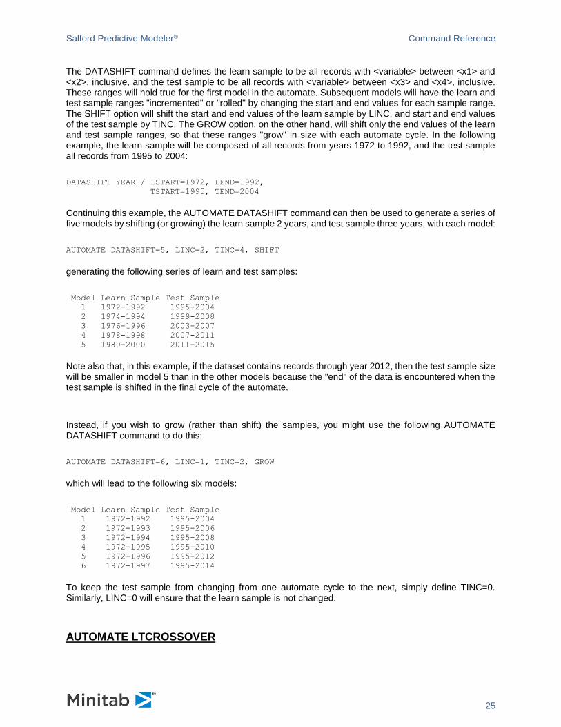
The DATASHIFT command defines the learn sample to be all records with <variable> between <x1> and <x2>, inclusive, and the test sample to be all records with <variable> between <x3> and <x4>, inclusive. These ranges will hold true for the first model in the automate. Subsequent models will have the learn and test sample ranges "incremented" or "rolled" by changing the start and end values for each sample range. The SHIFT option will shift the start and end values of the learn sample by LINC, and start and end values of the test sample by TINC. The GROW option, on the other hand, will shift only the end values of the learn and test sample ranges, so that these ranges "grow" in size with each automate cycle. In the following example, the learn sample will be composed of all records from years 1972 to 1992, and the test sample all records from 1995 to 2004:
DATASHIFT YEAR / LSTART=1972, LEND=1992,
TSTART=1995, TEND=2004
Continuing this example, the AUTOMATE DATASHIFT command can then be used to generate a series of five models by shifting (or growing) the learn sample 2 years, and test sample three years, with each model:
AUTOMATE DATASHIFT=5, LINC=2, TINC=4, SHIFT
generating the following series of learn and test samples:
Model Learn Sample Test Sample
1 1972-1992 1995-2004
2 1974-1994 1999-2008
3 1976-1996 2003-2007
4 1978-1998 2007-2011
5 1980-2000 2011-2015
Note also that, in this example, if the dataset contains records through year 2012, then the test sample size will be smaller in model 5 than in the other models because the "end" of the data is encountered when the test sample is shifted in the final cycle of the automate.
Instead, if you wish to grow (rather than shift) the samples, you might use the following AUTOMATE DATASHIFT command to do this:
AUTOMATE DATASHIFT=6, LINC=1, TINC=2, GROW
which will lead to the following six models:
Model Learn Sample Test Sample
1 1972-1992 1995-2004
2 1972-1993 1995-2006
3 1972-1994 1995-2008
4 1972-1995 1995-2010
5 1972-1996 1995-2012
6 1972-1997 1995-2014
To keep the test sample from changing from one automate cycle to the next, simply define TINC=0. Similarly, LINC=0 will ensure that the learn sample is not changed.
AUTOMATE LTCROSSOVER

Salford Predictive Modeler® Command Reference
26
Used with the LTCROSSOVER command, AUTOMATE LTCROSSOVER "shifts" the "crossover point" between learn and test samples with each cycle of the Automate. Think of the learn and test samples as being separated by a "sliding threshold value". Records with a value below the threshold are initially in the learn sample, otherwise they are in the test sample. As the Automate progresses, the threshold is shifted by INCREMENT. In this way the learn sample will (typically) grow and the test sample will shrink during the course of the Automate (although the LWIDTH and TWIDTH options on the LTCROSSOVER command will affect this).
AUTOMATE LTCROSSOVER=<n> [ INCREMENT=<x> ]
AUTOMATE TNREG
TreeNet regression only. AUTOMATE TNREG varies the TreeNet regression modes and the breakdown parameter. LAD is used first, the LS, then a series of Huber-M models using a default set of breakdown parameters: 0.98, 0.95, 0.90, 0.85:
AUTOMATE TNREG [ VALUES=<x1,x2,...>, REPEAT=<N> ]
REPEAT will repeat the experiment with different random seeds.

Salford Predictive Modeler® Command Reference
27
AUTOMATE TNRGBOOST
TreeNet regression only. AUTOMATE TNREG varies the TreeNet regression modes and the breakdown parameter. LAD is used first, then LS, then a series of Huber-M models using a default set of breakdown parameters: 0.98, 0.95, 0.90, 0.85.
AUTOMATE TNRGBOOST [ PERCENTILES=<YES|NO>,
L0=<p1,p2,...>, L1=<p1,p2,...>, L2=<p1,p2,...>,
ZEROBASELINE=<YES|NO>, LIST=<YES|NO> ]
When PERCENTILES=YES, which is the default, the AUTOMATE first generates a test run in which the penalties are all set to 0 to determine ranges of values large enough to induce a change in the model. The values specified on the command are percentiles of these baseline model values. Thus AUTOMATE TNRGBOOST L2=25,50,75
would impose L2 penalties of the 25th, 50th, and 75th percentile of plausible values discovered in the baseline model. If values are given for more than one penalty type (e.g. L1 and L2) then the AUTOMATE will perform the "full factorial" experiment: building models for all possible combinations of the specified percentiles. Percentiles are expected in the range [0,100]. Values less than 1.0 are understood to be percentiles and multiplied by 100. If you wish to list explicit values for L0, L1, L2 (rather than percentiles), use PERCENTILES=NO. In this case, the first test model is not needed and won't be built. If a baseline test model is built, the values for L0, L1 and L2 are forced to be 0.0. This is the recommended approach. In subsequent models, L0, L1 and L2 are either controlled by the automate logic if specified on the AUTOMATE TNRGBOOST command, or will take on values specified by the L0, L1 and L2 options on the TREENET command. If you do not wish them to be forced to 0.0 in the baseline test model, use ZEROBASELINE=NO. If no baseline test model is built (i.e., PERCENTILES=NO) then ZEROBASELINE has no effect. If PERCENTILES=YES, if you would like to view the ranges of regularization values determined in the baseline test model, set LIST=YES. The default is LIST=YES. LIST has no effect if PERCENTILES=NO. If you specify no values for L0, L1, and L2, then the default is to use the quartiles of each: AUTOMATE TNRGBOOST L0=25,50,75, L1=25,50,75, L2=25,50,75
along with zero values for a total of 4 x 4 x 4 = 64 models. If you wish to have the L0, L1 and L2 values randomly selected across a broad range of acceptable values, use the RANDOMSEARCH option: AUTOMATE TNRGBOOST RANDOMSEARCH=<N> [ RANDOMSEED=<M> ]
This will result in N+1 models being built. A first model will be built to determine plausible values for L0, L1 and L2, and N more models will be built using random combinations of those values. Specifying a different RANDOMSEED value allows you to repeat the experiment with the same number of models but a different group of randomly selected L0, L1 and L2 combinations.
Salford Predictive Modeler® Command Reference
28
AUTOMATE TNCLASSWEIGHTS
TreeNet only. varies class weights between UNIT and and BALANCED in N steps, for binary TreeNet models. The command syntax is:
AUTOMATE TNCLASSWEIGHTS [ = <N>, SAVE="filename" ]
The default is N=2, which builds only two models: UNIT and BALANCED. N must be 2 or greater.
AUTOMATE REFINE
CART classification only. AUTOMATE REFINE removes misclassified records from the learn sample and repeatedly rebuilds the model. The default number of refinement passes is 5.
AUTOMATE REFINE [ REPEAT=<n> ]
AUTOMATE ROOT
CART only. AUTOMATE ROOT builds CART trees with the root splitter forced according to the list of splitters:
AUTOMATE ROOT=<variable_list>
For example, the following will build four trees, each being split on one of the listed predictors (provided a split can be formed):
AUTOMATE ROOT=COUNTRY$,GENDER$,INCOME_GROUP,INCOME_AMOUNT
AUTOMATE ADDEDVAR
TreeNet only. AUTOMATE ADDEDVAR varies the ICL PENALTY value through a range of values:
AUTOMATE ADDEDVAR [ VALUES=<x1,x2,...>, REPEAT=<N> ]
If not specified, the default values are 0.0, 0.1, 0.2, 0.3, 0.4, and 0.5. REPEAT will repeat the experiment with different random seeds.
AUTOMATE OUTLIERS
Regression only. AUTOMATE OUTLIERS generates detailed univariate distributional reports for every continuous variable on the KEEP list. Intended to help uncover outliers and heavy-tailed distributions of variables.
AUTOMATE OUTLIERS
REGRESS GO
Salford Predictive Modeler® Command Reference
29
AUTOMATE RFNPREDS
RandomForests only. AUTOMATE RFNPREDS varies the number of potential splitters at a node in RandomForests. REPEAT will repeat the experiment with different random seeds.
AUTOMATE RFNPREDS [ VALUES=<n1,n2,n3,...>, REPEAT=<N> ]
If you have many predictors (e.g., hundreds or thousands), you can specify the number of potential splitters as a function of the square root of the total number of predictors, e.g.:
AUTOMATE RFNPREDS VALUES=1,2,EIGHTHSQR,4,SQR,12,SQRX2,BAGGER,ALL
in which the following tokens are available:
EIGHTHSQR - 1/8 of the square root of the total number of predictors
QUARTERSQR - 1/4 of the square root of the total number of predictors
HALFSQR - 1/2 of the square root of the total number of predictors
SQR - square root of the total number of predictors
SQRX2 - twice the square root of the total number of predictors
BAGGER - twice the square root of the total number of predictors
ALL - twice the square root of the total number of predictors
If there are fewer than 64 predictors, these options will instead be treated as: 1 (EIGHTHSQR), 2 (QUARTERSQR), 4 (HALFSQR), 8 (SQR) and 16 (SQRX2).
If there are more than 64 predictors, the default is:
AUTOMATE RFNPREDS VALUES=EIGHTHSQR,QUARTERSQR,HALFSQR,SQR, SQRX2
If there are 64 or fewer predictors, the default is:
AUTOMATE RFNPREDS VALUES=1,2,4,7,11
AUTOMATE UNSUPERVISED
CART only. AUTOMATE UNSUPERVISED generates a series of N unsupervised learning models.
AUTOMATE UNSUPERVISED=<n>
The default number of models is 10.
AUTOMATE GLM
AUTOMATE GLM produces an initial TreeNet model, forms a revised keep list of the “core” predictors and the <nkeep> most important noncore predictors, and models the revised keep list in all available modeling engines appropriate to the target type.
AUTOMATE GLM [ KEEP=<nkeep>, CORE=<corelist>, BIN=<YES|NO> ]
The defaults are:
AUTOMATE GLM KEEP=15
The BIN option determines whether predictors are auto-binned or not. If the data are auto-binned, by default

Salford Predictive Modeler® Command Reference
30
three sets of models will be built using the original predictors, binned predictors and bins in turn (the initial TreeNet model is built on binned predictors). Details of the auto-binning can be controlled with the BIN command:
BIN METHOD=<CART|EQUALFRACTION|EQUALWIDTH>, ORIGINAL=<YES|NO>,
BIN=<YES|NO>, FILLED=<YES|NO>
AUTOMATE EVERYTHING
AUTOMATE EVERYTHING is similar to AUTOMATE MODELS in that a model is built in each possible data mining engine. However, when used in conjunction with the BIN command, AUTOMATE EVERYTHING will build a model in each engine using predictors of each of the selected binning modes. For example:
BIN ORIGINAL=<YES|NO>, BIN=<YES|NO>, FILLED=<YES|NO>
AUTOMATE EVERYTHING
CART GO
The above will build three models in each engine: one on original predictors, one on binned (filled) predictors, and one on the bin assignments. Note: The AUTOMATE BIN_VAR_MODELS command is a synonym for the AUTOMATE EVERYTHING command.
AUTOMATE UPLIFT
Formerly Automate UPLIFT. Produces a series of three TreeNet models, making use of the TREATMENT variable specified on the TREENET command. The first model is built on just the treatment group records (records for which the TREENET TREATMENT variable is nonzero), the second model is built on just control group records (for which the TREENET TREATMENT variable is zero), and the third model is built on all records using a derived binary "XOR" target while making use of case weights that balance the data according to the TREENET WEIGHT option. The SAVE option will create a utility dataset that includes the derived target, model predictions, uplift probability and all forms of the case weights.
AUTOMATE DIFFLIFT [ SAVE=<"filename.ext"> ]
AUTOMATE RFBOOTSIZE
Formerly Automate RFBOOTSTRAP. AUTOMATE RFBOOTSTRAP varies the bootstrap sample size. The <p> values are proportions of the learn sample size:
AUTOMATE RFBOOTSIZE [ VALUES=<p1>,<p2>,..., REPEAT=<N> ]
The default is:
AUTOMATE RFBOOTSTRAP VALUES=0.01,0.05,0.10,0.25,0.50
In the above, 0.0 denotes no special handling (i.e., bootstrap size is equal to the learn sample size), 0.01 denotes a bootstrap sample size that is 1% of the learn sample size, and so on. Value must be between 0.0 and 1.0 inclusive. REPEAT will repeat the experiment with different random seeds.
Salford Predictive Modeler® Command Reference
31
AUTOMATE TNQUANTILE
Varies the quantile value for TreeNet LAD models. The default is:
AUTOMATE TNQUANTILE VALUES=0.01,0.25,0.50,0.75,0.90
Values must be between 0.0 and 1.0 exclusive. AUTOMATE TNQUANTILE is supported for continuous targets only. REPEAT will repeat the experiment with different random seeds.
AUTOMATE TNQUANTILE [ VALUES=<p1>,<p2>,..., REPEAT=<N> ]
AUTOMATE BIASPENALTY
AUTOMATE BIASPENALTY supports grid searches for optimal settings of the Bias Penalty control. CART and RF only. The command syntax is:
AUTOMATE BIASPENALTY [ ALPHA=<x1,x2,...>,
HLC1=<x1,x2,...>,
HLC2=<x1,x2,...>, REPEAT=<n> ]
The ALPHA, HLC1 and HLC2 options correspond to the three parameters of the PENALTY / BIAS control. ALPHA and HLC1 values should range from 0.0 to 1.0 inclusive. HLC2 values should range from 0.0 to 10.0 inclusive. If you specify no values for ALPHA, the default is to use values of 0.0, 0.25, 0.5, 0.75 and 1.0 If you specify no values for HLC1, the default is to use values of 0.1, 0.4, 0.7, and 1.0 If you specify no values for HLC2, the default is to use values of 0.5, 1.0 and 2.0 If you are using a randomly selected test partition, REPEAT will run each bias penalty scenario multiple times with the LEARN/TEST samples randomly repartitioned. If you wish to define separate penalty parameters for continuous versus categorical predictors, use the following syntax instead:
AUTOMATE BIASPENALTY [ CONTALPHA=<x1,x2,...>,
CONTHLC1=<x1,x2,...>,
CONTHLC2=<x1,x2,...>,
CATALPHA=<x1,x2,...>,
CATHLC1=<x1,x2,...>,
CATHLC2=<x1,x2,...>, REPEAT=<n> ]
You must either specify common values for bias penalties (e.g., ALPHA, HLC1, HLC2) or type-specific values (e.g., CONTALPHA, CONTHLC1, CONTHLC2, CATALPHA, CATHLC1, CATHLC2), but not both. If you wish to have the bias penalty values randomly selected across a broad range of acceptable values, use the RANDOMSEARCH option:
AUTOMATE BIASPENALTY RANDOMSEARCH=<N> [ RANDOMSEED=<M>, REPEAT=<R> ]
This will result in N models being built, using ALPHA and HLC1 values ranging from 0.0 to 1.0, and HLC2 values ranging from 0.0 to 5.0. Specifying a different RANDOMSEED value allows you to repeat the experiment with the same number of models but a different group of randomly selected bias penalty values.
Salford Predictive Modeler® Command Reference
32
AUTOMATE TNOPTIMIZE
AUTOMATE TNOPTIMIZE varies core TreeNet modeling parameters through a series of randomly selected values:
AUTOMATE TNOPTIMIZE [ RANDOMSEARCH=<N>, RANDOMSEED=<M>, REPEAT=<R> ]
This will result in N models being built. Specifying a different RANDOMSEED value allows you to repeat the experiment with the same number of models but a different group of randomly selected TreeNet parameters. REPEAT will repartition the learn/test samples and rerun the experiment. The default is RANDOMSEARCH=50.
AUTOMATE BIN_VAR_MODELS
Purpose
Similar to AUTOMATE MODELS in that a model is built in each possible data mining engine (CART, TreeNet, MARS, RandomForests, etc.). However, when used in conjunction with the BIN command, AUTOMATE BIN_VAR_MODELS will build a model in each engine for each using predictors of each of the selected binning modes. For example:
BIN ORIGINAL=<YES|NO>, BIN=<YES|NO>, FILLED=<YES|NO>
AUTOMATE BIN_VAR_MODELS
CART GO
will build three models in each engine: one on original predictors, one on binned (filled) predictors and one on the bin assignments. Note: The AUTOMATE BIN_VAR_MODELS command is a synonym for the AUTOMATE EVERYTHING command.

Salford Predictive Modeler® Command Reference
33
ANOMOLY
Purpose
The ANOMOLY command performs anomaly (outlier) detection. For each variable in the KEEP list (by default, all variables), the univariate distribution is determined. The percentile of each data point is determined and mapped to a score in the range [-.5, .5]. The product of scores for each variable is taken to determine the anomaly score for the entire data record. The command syntax is:
ANOMALY [ GO, SAVE="filename", REPORT=<yes|no>, MODEL=<yes|no>,
MISSING=<HIGH|LOW|OMIT> ]
SAVE will save your data, along with the anomaly score, the record's case weight and the data sample (learn/test/holdout) to an output dataset.
REPORT will describe the distribution of the anomaly score, separately for learn, test and holdout samples.
MODEL will build regression models of the anomaly score, using CART, TreeNet, MARS, Random Forests, GPS and linear regression in an effort to interpret why records might be outliers.
MISSING controls whether missing values are treated as "low" (extremely negative), "high" (extremely positive) or are omitted from computations of anomaly scores. The default is MISSING=OMIT.
By default the ANOMALY command considers all the variables in your dataset, but will be restricted to your KEEP list if you have one. The syntax is
AUXILIARY
Purpose
CART only. The AUXILIARY command specifies variables (either in the model or not) for which node-specific statistics are to be computed in a CART tree. For continuous variables, statistics such as N, mean, min, max, sum, SD and percent missing may be computed. Which statistics are actually computed is specified with the DESCRIPTIVE command. For discrete/categorical variables, frequency tables are produced showing the most prevalent seven categories.
The command syntax is:
AUXILIARY <variable>, <variable>, ...
Variable groups may be used in the AUXILIARY command similarly to variable names.
Closely related to AUXILIARY is the AUXRATIO command. The AUXRATIO command allows you to specify a pair of continuous variables for which the ratio of the means and sums of each pair will be reported in each terminal node of a CART tree. AUXRATIO affects CART models only.
Salford Predictive Modeler® Command Reference
34
AUXRATIO
Purpose
The AUXRATIO command allows you to specify a pair of continuous variables for which the ratio of the means and sums of each pair will be reported in each terminal node of a CART tree. Affects CART models only. The syntax is
AUXRATIO <variable1>,<variable2>
In which exactly two continuous variables must be specified.
BIN
Purpose
The BIN command bins the variables in your KEEP list. It is used in two ways. In conjunction with the AUTOMATE BIN command, the BIN GO starts the binning process. The command syntax is:
AUTOMATE BIN ... <options> ...
BIN GO
Binning options are specified on the AUTOMATE BIN command. For example, to bin your data using all default options:
USE "dataset.xls"
CATEGORY REGION, GENDER, ZIPCODE
BIN GO
When using AUTOMATE BIN and BIN GO, the goal is usually to produce a new output dataset with binned versions of your original variables.
You can also "auto-bin" variables immediately before modeling by using the BIN command with appropriate options:
BIN METHOD=<CART|EQUALFRACTION|EQUALWIDTH|ROUND=<N>|ADAPTIVEROUND=<N>>,
ORIGINAL=<yes|no>,
FILLED=<yes|no>, BIN=<yes|no>, CODING=<MEAN|WOE>,
FILL=<variable>, GROUP=<variable>, SUPERVISE=<variable>,
IDEALBINS=<n>, LAPLACE=<0.5|1.0>, PREFER=<MORE|FEWER>,
REPORT=<SHORT|LONG>, SMALLESTBIN=<N>
For example, to construct equally populated bins of all predictors and then to build three CART models on the original, filled and bin assignments, use the commands:
BIN METHOD=EQUALFRACTION, ORIGINAL, FILLED, BIN
To bin the predictions using weights of evidence coding (which requires a categorical FILL variable) and then to build two TreeNet models using original and filled (weights of evidence) versions, use the commands:
CATEGORY FILLCODEVAR
BIN ORIGINAL, FILLED, CODING=WOE, FILL=FILLCODEVAR
TREENET GO
Salford Predictive Modeler® Command Reference
35
The defaults are:
BIN METHOD=EQUALFRACTION, ORIGINAL, FILLED, BIN, CODING=MEAN,
IDEALBINS=10, LAPLACE=1.0, PREFER=FEWER, REPORT=LONG,
SMALLESTBIN=0
Note: the SUPERVISE option is only meaningful if METHOD=CART.
AUTOMATE BIN_VAR_MODELS
Similar to AUTOMATE MODELS in that a model is built in each possible data mining engine (CART, TreeNet, MARS, RandomForests, etc.). However, when used in conjunction with the BIN command, AUTOMATE BIN_VAR_MODELS will build a model in each engine for each using predictors of each of the selected binning modes. For example:
BIN ORIGINAL=<YES|NO>, BIN=<YES|NO>, FILLED=<YES|NO>
AUTOMATE BIN_VAR_MODELS
CART GO
will build three models in each engine: one on original predictors, one on binned (filled) predictors and one on the bin assignments.
BLOCK
Purpose
The BLOCK command defines one or more variables that define a "block" of records. BLOCK currently only affects how lags are created, i.e., lags are reset when a record exhibits a changed value in one or more of the BLOCK variables. In this way, case histories can be defined by identifying variables that remain constant throughout the case history. The command syntax is:
BLOCK <variable1> [, <variable2>, <variable3>, ... ]
For example, you might build a CART model involving current and lagged values of PRICE and RATE. By using the BLOCK command, you can specify that the lags should be reset when a new customer ID is encountered:
MODEL TARGET
KEEP ..., PRICE<0-3>, RATE<0-4>, ...
BLOCK ID
CART GO
Salford Predictive Modeler® Command Reference
36
BOPTIONS
Purpose
The BOPTIONS command allows a variety of advanced parameters to be set. The command syntax is:
BOPTIONS SERULE=<x>, COMPLEXITY=<x>, COMPETITORS=<n>, CPRINT=<n>,
SPLITS=<n|AUTO>, SURROGATES=<n1>, PRINT=<n2>, OPTIONS,
NCLASSES=<n>,MCLASSES=<m>, CVLEARN=<n>, NOTEST, ECHO, TREELIST=<n>,
PAGEBREAK=<"page_break_string">,
NODEBREAK=<ALL|EVEN|ODD|NONE|<N>>, NBINS=<N>, NDECILES=<N>,
IMPORTANCE=<x>, COPIOUS | BRIEF, SCALED,
QUICKPRUNE=<YES|NO>, DIAGREPORT=<YES|NO>, MAXHLC=<n>,
HLC=<n1>,<n2>, PLC=<YES|NO>, CVS=<YES|NO>,
PROGRESS=<SHORT|LONG|NONE>, OLS=<YES|NO|ONLY>,
MISSING=<YES|NO|DISCRETE|CONTINUOUS|LIST=varlist>,
MREPORT=<YES|NO>, VARDEF=<N|1>, MARSRIDGE=<x>, MAXNREPORT=<n>,
CTHRESHOLD=<DATA|x>, LTHRESHOLD=<x>, CARDINAL=<n1,n2,n3>,
FULLSAVE=<YES|NO>, LEARNBINS=<n>, TESTBINS=<n>
in which <x> is a fractional or whole number and <n> is a whole number.
SERULE the number of standard errors to be used in the optimal tree selection rule. The default is 0.0.
COMPLEXITY parameter limiting tree growth by penalizing complex trees. The default is 0.0 -- no penalty, trees grow unlimited.
COMPETITORS number of competing splits stored for each node, and reported in GUI reports. Default=5.
CPRINT number of competing splits printed for each node in the classic (text) output. Defaults to the COMPETITORS option.
SPLITS forecast of the number of splits (primary and surrogate) on categorical variables in maximal tree. This value is automatically estimated by CART but may be overridden.
SURROGATES <n1> is maximum number of surrogates to store for the tree and upon which to compute variable importance. Default= 5.
PRINT <n2> is the number of surrogates to report for each node, and is set equal to <n1> if not specified.
OPTIONS report of advanced control parameters at end of tree building.
NCLASSES For classification problems in which the number of dependent levels is greater than 2, NCLASSES specifies the maximum number of classes allowed for an independent categorical variable for an exhaustive split search. For independent categorical variables with more levels, special 'high-level categorical' algorithms are used (see the HLC option). Depending on the platform, for classification problems NCLASSES greater than 10-20 can result in significant increases in compute time. The default is 15. NOTE: for BINARY classification trees, special algorithms are used that allow exhaustive split searches for high level categorical predictors with essentially no compute-time penalty.
MCLASSES sets a threshold for the maximum allowable number of classes for a categorical predictor. Any predictor having more than MCLASSES classes will not be considered as a splitter in the CART model. The default is 1024. Note that for classification trees, one part of the memory required to build the tree scales with the square of the greatest number of classes found

Salford Predictive Modeler® Command Reference
37
among all categorical predictors, so if you encounter memory allocation problems trying to build a CART model with a categorical target and high-level-categorical predictors, consider lowering the MCLASSES setting.
NBINS sets the number of bins for gains charts and uplift tables in the classic output. The default is 10. Allowable values are 2 to 100.
NDECILES sets the number of bins for deciles of risk (Hosmer-Lemeshow) tables in classic output. The default is 10. Allowable values are 2 to 100.
CVLEARN the maximum number of cases allowed in the learning sample before cross-validation is disallowed and a test sample required. The default is 3000.
TREELIST number of trees reported in tree sequence summary. Default=10. The optimal and maximal trees are also shown.
PAGEBREAK defines a string that may be used to mark page breaks for later processing of CART text output. The page break string may be up to 96 characters long, and will be inserted before the tree sequence, the terminal node report, learn/test tables, variable importance and the final options listing. Page breaks are also inserted in the node detail output, according to the NODEBREAK options (see below). If the pagebreak string is blank, no pagebreaks are inserted.
NODEBREAK This option is only active if you have defined a nonblank pagebreak string with the PAGEBREAK option. NODEBREAK allows you to specify how often the node detail report is broken by page breaks. The options are ALL, EVEN, ODD, NONE or you may specify a number (such as 3 or 10). The default is ODD, breaking prior to node 3, 5, etc. Even if you request NONE, there will still be a pagebreak prior to the node detail title.
IMPORTANCE weight on surrogate improvements when calculating variable importance. Must be between 0 and 1. The default is 1.0.
COPIOUS | BRIEF| SCALED COPIOUS reports detailed node information for all maximal trees grown in cross validation. The default is BRIEF. SCALED indicates the complexity specified IS NOT relative. Any complexity specified as greater than 1.0 is considered scaled and the SCALED option is not required.
QUICKPRUNE invokes an algorithm that avoids rebuilding the tree after pruning has selected an optimally-sized tree.
DIAGREPORT produces tree diagnostic reports.
MAXHLC Sets a threshold on the maximum number of classes that a categorical predictor is permitted to have in REGRESS, RIDGE and LOGIT models. These models create “dummies” for each predictor class so the dimensionality of the model can become overwhelming if a high-level categorical predictor is attempted. The default value is 300.
HLC Accommodation for high cardinality categoricals. Assume the variable in question has nlev levels: n1: number of initial random split trials (<n1> must be greater than 0.). n2: number of refinement passes. Each pass involves nlev trials. <n2> must be greater than 0. The default is HLC=200,10. The HCC option is identical to HLC.
PLC controls whether linear combinations other than the primary splitter are included in the node-by-node detail report.
CVS controls whether CV trees are saved in the GROVE.
Salford Predictive Modeler® Command Reference
38
PROGRESS Issues a progress report as the initial tree is built. This option is especially useful for trees that are slow to grow. LONG produces full information about the node, SHORT produces just the main splitter info, and NONE turns this option off. The default is NONE.
OLS controls whether OLS results are presented during a MARS model.
MREPORT produces a special report summarizing the amount of missing data in the learn and test samples.
MISSING adds missing value indicators to the model. It has several forms. NO disables missing value indicators. YES will produce missing value indicators for all predictors in the model that have missing values in the learn sample. DISCRETE will produce missing value indicators only for discrete predictors. CONTINUOUS will do so only for continuous predictors. LIST= specifies a list of variables; those in the list that appear as predictors in the model and have missing values in the learn sample will get missing value indicators. LIST= can include variable groups and variables that are not part of the model.
VARDEF specifies whether a denominator of N or N-1 should be used in variance and standard deviation expressions in regression trees. The default is N, which is what the original CART implementation used.
MARSRIDGE maintains MARS numerical stability. Default value is 1.e-7.
MAXNREPORT Sets a limit on the number of variables, or items, in some reports that can become quite lengthy when there are many variables. The default is 1000. A value of 0 denotes no limit.
CTHRESHOLD determines the probability threshold for separating classes when computing classification error rates. The default is 0.5. DATA bases the threshold on the learn sample target distribution. The range is 0.0 - 1.0 exclusive (0.0 and 1.0 are not permitted). Binary models only.
LTHRESHOLD determines the threshold for computing lift. The default is 0.1. The range is 0.0 (excluded) to 1.0.
CARDINAL controls the "cardinality report" summarizing the dimensionality of any discrete variables involved in the model. The cardinality report includes an EXCLUDE command for variables with the largest number of levels. All three options are required. N1 limits the number of variables listed in the report, N2 limits the number of variables in the EXCLUDE command, and N3 is a minimum number of levels a variable must exhibit to be included in the report. The default values are 100, 100, and 3. In other words, the 100 highest dimensionality variables will be listed, omitting binary discrete variables.
FULLSAVE controls whether node detail is saved in CART trees. The default is FULLSAVE=YES except for CART trees built by AUTOMATE MCT, in which case the node detail in the null model trees is normally not saved. To preserve it, use FULLSAVE=YES. This will increase resource requirements for visualizing, translating or scoring these models. FULLSAVE only affects CART models.
LEARNBINS specify the number of bins used when constructing the residual model fit diagnostics tables for regression models. The default is 20. Allowable values are 2 to 200.
TESTBINS specify the number of bins used when constructing the residual model fit diagnostics tables for regression models. The default is 20. Allowable values are 2 to 200.
Salford Predictive Modeler® Command Reference
39
Some examples are:
BOPTIONS SERULE=.85, COMPETITORS=50, CPRINT=10, SURROGATES=10,
COPIOUS, LIST
BOPTIONS SPLITS=90, SURROGATES=8 PRINT=3, SERULE=0, OPTIONS
The BOPTIONS command also controls a variety of options associated with MARS:
BOPTIONS INTERACTIONS=N, BASIS=N, CRASTER=N, SRASTER=N,
PLOT=LINEAR|CUBIC, MINSPAN=N, SPEED=N, PENALTY=X,
HEIGHT=N, WIDTH=N, MARS2=YES|NO
INTERACTIONS set the allowable number of interactions between variables. The default is 1.
BASIS set the basis functions maximum. The default is 40.
CRASTER set the number of raster points for curves.
SRASTER set the number of raster points on each axis for surfaces.
MINSPAN set the minimum number of observations between each knot. The default is 0.
SPEED speed acceleration factor (1-5).Larger values progressively sacrifice optimization thoroughness for computational speed advantage usually resulting in marked decrease in computing time with little or no effect on resulting approximation accuracy (especially useful for exploratory work). 1 = no acceleration; 5 = maximum speed advantage; the default is 4.
PENALTY Fractional incremental penalty for increasing the number of variables in the mars model. Sometimes useful with highly collinear designs to produce nearly equivalent models with fewer predictor variables, aiding in interpretation. Must assume nonnegative values only. The default is 0. 0.05 is a moderate penalty, 0.10 is a heavy penalty. The best value depends on the specific situation and some user experimentation using different values is usually required. This option should be used with some care.
HEIGHT Height, in lines, of the low-res response plots. Allowable values are 17 to 57, inclusive.
WIDTH Width, in characters, of the low-res response plots. Allowable values are 60 to 110, inclusive.
PLOT specifies whether MARS should low-res plot the linear or cubic form of the model.
MARS2 specifies whether certain computational idiosyncrasies are handled as in MARS v. 2. Setting this option may help produce results that better match those of MARS v2. For normal use, it is recommended that this option be left off (MARS2=NO).

Salford Predictive Modeler® Command Reference
40
BOSS - Bias Optimized Shrinkage and Selection
Purpose
The BOSS command controls the Bias Optimized Shrinkage and Selection of CART regression trees. P, Q, and R range from 0.0 and 1.0 inclusive. The command syntax is:
BOSS = NO
BOSS = <P,Q,R> [ REPORT=NO|SHORT|LONG, DIAG=NO|SHORT|LONG,
GRIDSEARCH=YES|NO, DEGREE=<n> ]
To invoke BOSS, use the syntax BOSS=P,Q,R as follows:
Q power on standard deviation of target in node (learn sample). Most typical values to use are 0, .5, and 1.
Q=0 is recommended for discrete dependent variables and makes no adjustments based on target variance
Q=.5 makes adjustments based on the standard deviation of the target
Q=1 makes adjustments based on the variance of the target
Q>0 and <=.25 may be helpful for heteroscedasticity of target conditional on predictor values
P power on relative shares of learn data going to left and right children of the split. For most problems we recommend P=0. If P is non-zero it should be set following the rules below.
R power on the sample size of the node being split. For most problems we recommend R=0.
P,R combinations. Trying values which sum to .5 could be useful. Suggestions include P=0, R=.5 and P=.5, R=0.
Q=1, P=1, R=0 Is designed to mimic ridge regression
Q=.5, P=0, R=0 uses common shrinkage for all nodes (state of the art prior to BOSS).
Examples:
BOSS=0,0,0 constant shrinkage
BOSS=0,.5,0 recommended starting point for typical regression
BOSS=.5,0,0 recommended for discrete dependent variables
BOSS=1,1,0 ridge-like regression tree
To suppress BOSS processing:
BOSS=NO
BOSS is suppressed by default.
Following the BOSS parameters:
REPORT and DIAG options control reporting of BOSS results. Basic reporting is controlled with the REPORT=NO|SHORT|LONG option. Diagnostic reporting is controlled with DIAG=NO|SHORT|LONG option. GRIDSEARCH=YES, DEGREE=<n> will perform a nxnxn grid search over the range of all three BOSS parameters, reporting holdout SSE reduction and the "best" BOSS parameters.
Salford Predictive Modeler® Command Reference
41
BOSS=<P,Q,R> [ REPORT=NO|SHORT|LONG, DIAG=NO|SHORT|LONG,
GRIDSEARCH=YES|NO, DEGREE=<n> ]
Basic BOSS reporting is controlled with REPORT=NO|SHORT|LONG. Extended diagnostic reporting is controlled with DIAG=NO|SHORT|LONG. GRIDSEARCH=YES, DEGREE=<N> will perform a NxNxN grid search over the range of all three BOSS parameters, reporting holdout SSE reduction and the "best" BOSS parameters.
CART
Purpose
The CART command builds a CART model. The command syntax is:
CART [ GO, MCLASSES=<n>,
REGEVAL=NONE|OPTIMAL|ALL|<N>,
LOGEVAL=NONE|OPTIMAL|ALL|<N>,
CATCONSISTENCY=YES|NO,
CVALIGN=YES|NO, CVQ2=<N> ]
MCLASSES sets a threshold for the maximum allowable number of classes for a categorical predictor. Any predictor having more than MCLASSES will not be considered as a splitter in the CART model. The default is 1024. Note that for classification trees, one part of the memory required to build the tree scales with the square of the greatest number of classes found among all categorical predictors, so if you encounter memory allocation problems trying to build a CART model with a categorical target and high-level-categorical predictors, consider lowering the MCLASSES setting.
CVALIGN, CVQ2 For CART models built using cross validation, the CVALIGN option will optionally produce a report detailing how the cross-validation trees are complexity-aligned for purposes of pruning and computing OOB performance measures, and the CVQ2 option will report the learn sample and OOB performance measures for the smallest <n> prunings. The defaults are CVALIGN=NO, CVQ2=50.
REGEVAL, LOGEVAL By default, performance measures are computed for the optimal pruning only for regression trees, and all prunings for binary classification trees. You can control for which prunings performance measures such ROC, gains, R-squared, outlier trimming tables, lift, etc. are computed: OPTIMAL for the one or more "optimal" prunings as determined by the CART algorithm, ALL for all prunings (this can be time consuming for regression models!), NONE for not at all, and <N> for all prunings with N or fewer terminal nodes.
For example, a classification CART tree:
USE "loans2000.xls"
MODEL DEFAULT
CATEGORY DEFAULT, PROPERTY_TYPE$, COUNTRY, INCOME_GROUP
KEEP LTV, REGION, AGE, PASTDUE<0-3>, RATE<0-3>, TAXES,
PROPERTY_TYPE$, COUNTRY, INCOME_GROUP
PARTITION TEST=.3
CART GO
CART differential lift (UPLIFT) Models

Salford Predictive Modeler® Command Reference
42
To build CART differential lift models designed to measure the difference in response between treated and untreated populations, use the TREATED, TARGET, WEIGHT and RESPONSE options on the CART
command. There are three ways to setup up UPLIFT model. The first approach:
MODEL <responded_variable>
UPLIFT TREATED=<treatment_variable>
CART GO
will use the <responded_variable> and <treated_variable> to construct an "xor" binary target, and will adjust weights in each partition based on treated/control and response groups. The second approach simply uses the RESPONSE option on the UPLIFT command in lieu of the MODEL command:
UPLIFT TREATED=<treated_variable>, RESPONSE=<responded_variable>
CART GO
Again, in the above approach a binary "xor" target will be constructed and used to estimate the model, with weights adjusted to balance group shares. The third approach employs three variables: a target, a responded/not variable and a treated/control variable:
MODEL <target_variable>
UPLIFT TREATED=<treated_variable>, RESPONSE=<responded_variable>,
TARGET=NATURAL
CART GO
In this case, no "xor" target is constructed; rather the model is built using the target named on the MODEL
command. However, the shares are still balanced by adjusting case weights. CART uplift models support four weighting modes, in which the group shares are balanced in each
partition (before it is split) by adjusting weights:
UPLIFT ... WEIGHT=<RESPONSE|TREATMENT|CROSS|QUAD> ...
TREATMENT balances treatment and control groups. RESPONSE balances responded/ not-responded
groups. CROSS balances both treated/control and responded/ not-responded groups. QUAD equalizes the
shares in all four quadrants.
Note: the treated and responded variables should be zero/nonzero, with nonzero values indicating treated and responded states, respectively. To turn off uplift modeling, using the UPLIFT=NO option.
CART CATCONSISTENCY=YES introduces a small change in the legacy CART engine for categorical splitters, to better align results with the new NMODEL CART engine when there are multiple split points for a categorical predictor in a given node that are tied on improvement. The default is CATCONSISTENCY=NO, which follows the conventions used in SPM 8.3 and earlier.
Salford Predictive Modeler® Command Reference
43
CATEGORY
Purpose
The CATEGORY commandindicates whether the target variable is categorical (thereby initiating a classification model) and identifies which predictors are categorical. For example,indicates whether the target variable is categorical (thereby initiating a classification model) and identifies which predictors are categorical. For example,
The command syntax is:
CATEGORY <var1>, <var2>
Examples:
MODEL LOW
CATEGORY LOW (categorical dependent variable indicates classification models) MODEL SEGMENT
CATEGORY SEGMENT
CATEGORY is also used to identify categorical predictor variables. SPM will determine the number of distinct values for you as your data are processed.
Example:
MODEL LOW
CATEGORY LOW, AGE, RACE, EDUC
Salford Predictive Modeler® Command Reference
44
CDF
Purpose
The CDF command evaluates one or more distribution, density, or inverse distribution functions at specified values.
For cumulative distribution functions the syntax is:
CDF [ NORMAL = z | T = t,dof | F = f,dof1,dof2 |
CHI-SQUARE = chisq,dof | EXPONENTIAL = x | GAMMA = gamma,p |
BETA = beta,p,q | LOGISTIC = x | STUDENTIZED = x,p,q |
WEIBULL = x,p,q | BINOMIAL = x,p,q | POISSON = x,p ]
To generate density values, use the syntax above with the DENSITY option:
CDF DENSITY [ distribution_name = user-specified-value(s) ]
To generate inverse cdf values, specify an 'alpha' value between 0 and 1:
CDF INVERSE [ NORMAL=alpha | T=alpha,dof | POISSON=alpha,p |
F=alpha,dof1,dof2 | CHI-SQUARE=alpha,dof |
EXPONENTIAL=alpha | GAMMA=alpha,p | BETA=alpha,p,q |
LOGISTIC=alpha | STUDENTIZED=alpha,p,q |
WEIBULL = alpha,p,q | BINOMIAL=alpha,p,q ]
For example:
CDF NORMAL=-2.16, DENSITY NORMAL=-2.5, INVERSE CHISQ=.8,3
CENSOR
Purpose
TreeNet only. The CENSOR command is used for survival analysis models and allows the model to distinguish complete (uncensored) from incomplete (censored) measures of the target variable. The command syntax is:
CENSOR <censoring variable>
The censoring variable must be coded as 0 for uncensored and 1 for censored.
Salford Predictive Modeler® Command Reference
45
CLASS
Purpose
The CLASS command assigns labels to specific levels of categorical variables (target or predictor). Labels are not limited in their length, although in some reports they will be truncated due to space limitations. For instance, if variable DRINK takes on the values 0, 1, 2, and 3 in the data, you might wish to assign labels to those levels:
CATEGORY DRINK
CLASS DRINK 0=tea 1='Columbian coffee' 2="soda pop",
3='Cold German Beer!'
Class labels will appear in most reports where variable levels are reported, in lieu of the levels themselves. It is not necessary to specify labels for all levels of a categorical variable -- any levels without a label will appear as the level itself. The command syntax is:
CLASS <variable> <level>=<string>, <level>=<string>, ...
You may issue separate CLASS commands for each variable, such as:
CLASS PARTY 1=Repub 2=Democratic 3="Peace and Freedom"
CLASS GENDER 0=female 1=male
CLASS EVAL$ "G"="Good", "F"="Fair", "P"="Poor"
or you may combine them in a single command, separating variables with a slash:
CLASS PARTY 1=Repub 2=Democratic,
3="Peace and Freedom" / GENDER 0=female 1=male /,
EVAL$ "G"="Good", "F"="Fair", "P"="Poor"
Note that the label "Peace and Freedom" requires quotes, since it contains spaces. Labels consisting only of numbers and letters can be listed without quotes, but if so any letters will be converted to uppercase.
Note also that all class labels for a given variable must be defined at once, since the <variable> token that leads the list of classes resets any existing class labels for the variable.
Variable groups that are composed of one type of variable only (i.e., numeric or character) may be used in the CLASS command similarly to variable names, e.g.:
GROUP CREDITEVAL = EVAL3MO, EVAL6MO, EVAL1YR, EVAL3YR
CATEGORY CREDITEVAL
CLASS CREDITEVAL 0="n/a", 1="Poor", 2="Fair", 3="Good"
Class labels are reset with the USE and NEW commands. They are preserved in a SPM grove file. To reset all class labels, issue the CLASS command with no options:
CLASS
To see a summary of class labels issue the command:
CLASS _TABLE_

Salford Predictive Modeler® Command Reference
46
CLUSTER
Purpose
The CLUSTER command initiates K-means clustering for the variables in your KEEP list. The command syntax is:
CLUSTER [ GO, K=<n>, ITERATIONS=<n>, REPORT=<LONG|SHORT>,
SEED=<SPREAD|KMEANS|RANDOM>, REPEAT=<N>, SAVECENTROIDS=<filename>, ]
STANDARDIZE=<YES|NO>
The default is:
CLUSTER NUMBER=2, ITERATIONS=50, REPORT=LONG, SEED=SPREAD
in which case 2 clusters will be computed (one split of the data). ITERATIONS controls how many iterations will be used (default of 50). REPORT=SHORT will suppress reporting of the cluster centroids in the classic output (default is LONG). SAVECENTROIDS will save the centroids (mean, min, max, stddev) to your output dataset. SEED=SPREAD uses a guided hierarchical algorithm to seed the clusters. SEED=KMEANS uses the KMeans++ distance-squared probability weighted approach to selecting random records to seed the clusters. SEED=RANDOM uses simple random selection of records to seed the clusters. REPEAT=<N>, when used with SEED=RANDOM or KMEANS, reclusters the data N times using different random record selections each time. STANDARDIZE will standardize the data before clustering, so that distances and optimal cluster solutions are based on standardized data, but final reporting will show solutions in terms of both original and standardized data and distance measures.
A note about the SEED options. Cluster seeding can have a profound impact on the cluster solution achieved. SEED=SPREAD tends to outperform KMEANS and RANDOM in terms of sum of squared distances, but SPREAD is not guaranteed to find the requested number of clusters. SEED=KMEANS tends to outperform SEED=RANDOM because the randomly selected seed centroids for SEED=KMEANS use squared distance to influence the randomness.
The REPEAT option can be used with SEED=KMEANS and SEED=RANDOM to increase the "search" for near-optimal seed centroids, at the cost of time.
The SEED=SPREAD algorithm initializes the first cluster to the sample mean. Successive clusters are then found iteratively in the following way: among the existing N clusters (N >= 1) the record that is most distant from the cluster to which it is currently assigned is removed from its cluster and becomes the centroid of the N+1'th cluster. Cluster-record assignments are determined anew on the N+1 clusters. The iteration is then repeated. When sufficient seed clusters have been found, the iterations are ended and classic KMeans clustering is done to refine the clusters. This approach provides a good alternative to KMeans-type seeding, but due to its hierarchical nature it is not guaranteed to find all the requested clusters.
When constructing clusters, the distance between a data record and a cluster centroid is found. This distance is the sum of squared differences between the centroid and the record, for all non-missing dimensions. The distance is normalized by the number of non-missing dimensions.
Note that the SAVECENTROIDS option is used to save cluster centroids, not cluster assignments, to an output dataset. Use the SAVE command to save the cluster assignments to an output dataset. For example, to save both cluster centroids and assignments, you might use the following:
USE <filename>
SAVE "assignments.csv"
CLUSTER GO, SAVECENTROIDS="centroids.csv"

Salford Predictive Modeler® Command Reference
47
COMBINE
Purpose
CART only. The COMBINE command launches a combined-tree or "ensemble" run, producing a model consisting of several or many CART trees. All options for COMBINE are set with a previous instance of the MOPTIONS. The command syntax is:
COMBINE GO
For example:
USE "loans2000.xls"
MODEL DEFAULT
CATEGORY DEFAULT, PROPERTY_TYPE$, COUNTRY, INCOME_GROUP
KEEP LTV, REGION, AGE, PASTDUE<0-3>, RATE<0-3>, TAXES,
PROPERTY_TYPE$, COUNTRY, INCOME_GROUP
MOPTIONS CYCLES=20, SETASIDE=SEPVAR=TESTRANDOM50P, TEST
GROVE "ensemble.grv"
COMBINE GO
USE "newloans.xls"
GROVE "ensemble.grv"
SCORE GO
Salford Predictive Modeler® Command Reference
48
CORR
Purpose
The CORR command computes symmetric triangular matrices of correlation, sums of products, covariance or similarity on two or more variables. Each option computes a different type of measure; they are discussed individually below. The results are displayed in a lower diagonal matrix of coefficients. Each coefficient (cell) in the matrix is labeled by the variable names at the beginning of its row and at the top of its column. Correlation matrices show a numeric association for every pairing of variables in a matrix arrangement. The command syntax is:
CORR <variable list> / <options>
If no variables are specified, CORR will either use all the variables in the dataset or those variables that are specified in the KEEP list (if there is one). The options are:
PEARSON produces a matrix of Pearson product moment correlation coefficients.
SPEARMAN produces a matrix of Spearman rank order correlation coefficients.
COVARIANCE produces a covariance matrix.
EUCLIDEAN produces a matrix of Euclidean distances normalized by the sample size.
CITY produces a matrix of City Block distances normalized by the sample size.
GAMMA produces a matrix of Gamma coefficients.
MU2 produces a matrix of Mu2 coefficients.
TAU produces a matrix of Kendall Tau-b rank order coefficients.
SSCP produces a sum of cross products matrix. If the PAIRWISE option is chosen, sums will be weighted by N/n, where n is count for a pair.
POSITIVE produces a matrix of positive matching dichotomous coefficients. Data are treated as zero/nonzero.
JACARD produces a matrix of Jaccard's dichotomous coefficients. Data are treated as zero/nonzero.
ANY produces a matrix of simple matching dichotomous coefficients. Data are treated as zero/nonzero.
ANDERBERG produces a matrix of Anderberg's dichotomous coefficients. Data are treated as zero/nonzero.
TANIMOTO produces a matrix of Tanimoto's dichotomous coefficients. Data are treated as zero/nonzero.
ALL produces all possible matrices. Be careful, it may be very time consuming!
N=<n> specifies that only the first <n> records should be used. This can be useful in exploratory analysis on very large datasets, especially for the GAMMA, SPEARMAN, MU2, TAU, and Sn methods for which the compute time scales exponentially with the amount of data.
WIDE prints matrices in 13-column reports.
LISTWISE imposes listwise deletion of missing data.
Salford Predictive Modeler® Command Reference
49
PAIRWISE imposes pairwise deletion of missing data, which requires an additional pass through the data.
By default, matrices are printed in segments with no more than 9 columns per segment. WIDE increases it to 13 columns per segment.
CSV
Purpose
The CSV command launches The CSV command defines options for reading comma-separated text datasets. Its has several forms:
CSV [ NMISSING="code1","code2",... ]
CSV [ CMISSING="code1","code2",... ]
CSV DEFAULT
NMISSING defines missing value codes for numeric variables. Each code must be quoted individually. CMISSING does the same for character variables. DEFAULT adds a set of commonly-used numeric variable missing value codes to any you may have already defined. Issuing the CSV command with no arguments:
CSV
clears all user-defined missing value codes and instantiates the default codes for numeric variables.
When .CSV files are created, you have some control over how floating point data points are formatted:
CSV OUTPUTPRECISION=DEFAULT|4|8|CLEAN|C8
The options are:
DEFAULT: uses the C format specifier %g
4: uses the C format specifier %f
8: uses the C format specifier %.16g
CLEAN: same as 8 but removes trailing 0's when possible
C8: uses the C++ function to_string(const double) for conversions
CW (Class Weights)
Purpose
TreeNet and RandomForests only. The CW command allows optional balancing of unequal class sizes via reweighting (class weights) for RandomForests and TreeNet models. CW does not affect any other model type in SPM.
CW [ BALANCE| UNIT | SPECIFY <class1>=<x1>, <class2>=<x2>, ... ]
in which <x1>, <x2>, ... is a vector of real numbers. The options set class weights as follows:
Salford Predictive Modeler® Command Reference
50
UNIT weights are unadjusted allowing class sizes to determine effective class weights. UNIT is the default for binary targets.
BALANCE small classes are upweighted to achieve balance with larger classes. The default setting for multinomial targets and recommended for most problems.
SPECIFY <class1>=<x1>,<class2>=<x2>,...
class weights set to any strictly positive numbers. A value must be assigned to each class. For character classes, the class value must be in quotes. The SPECIFY option requires that the target variable be previously identified on the MODEL command. Use CW SPECIFY to upweight those classes for which you want RandomForests or TreeNet to achieve higher rates of classification accuracy.
Examples:
CW BALANCE (the default for multinomial targets)
CW SPECIFY "COKE"=1, "Pepsi"=2,
"H2O"=4, "7UP"=1 (explicit list, let CART rescale)
CW UNIT (the default for binary targets)
NOTE: for RandomForests models, you can specify that the class weights be scaled to sum to some positive number with the RF SCW=<x> option.
DATA
Purpose
The DATA command defines block of BASIC statements that define new variables or modify existing variables. The BLOCK begins with a DATA command and ends with a DATA END command.
DATA
(BASIC programming statements here ...) DATA END
Typically, single BASIC statements are not contained within a "DATA block" but are instead preceded by a percent symbol, e.g.
%let test=urn>.8
However, when a group of BASIC statements is placed within a DATA block of commands, the percent symbol is not required. For example:
DATA
let gender$="Unknown"
if gcode=0 then let gender$="Female"
if gcode=1 then let gender$="Male"
let sample$="Learn"
if urn>.7 then let sample$="Test"
if urn>.85 then let sample$="Holdout"
DATA END
You may prefer to use the "percent symbol notation" as an alternative, in which case the above statements would look like this:
%let gender$="Unknown"
%if gcode=0 then let gender$="Female"
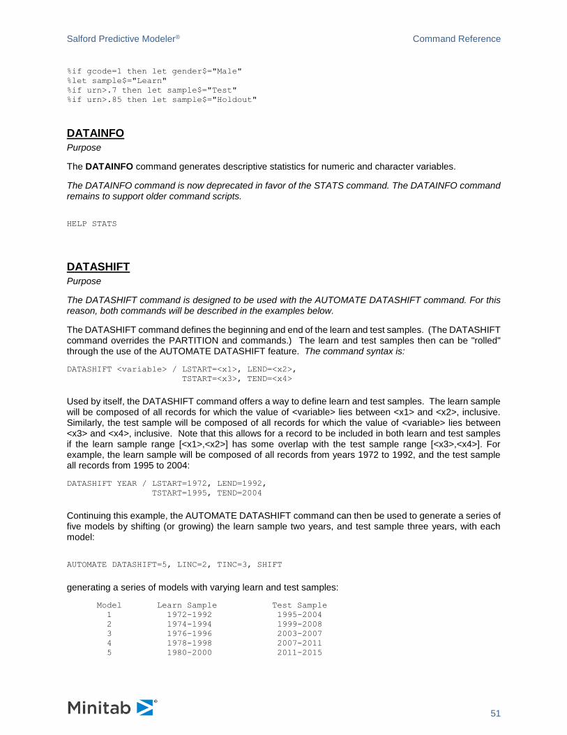
Salford Predictive Modeler® Command Reference
51
%if gcode=1 then let gender$="Male"
%let sample$="Learn"
%if urn>.7 then let sample$="Test"
%if urn>.85 then let sample$="Holdout"
DATAINFO
Purpose
The DATAINFO command generates descriptive statistics for numeric and character variables.
The DATAINFO command is now deprecated in favor of the STATS command. The DATAINFO command remains to support older command scripts.
HELP STATS
DATASHIFT
Purpose
The DATASHIFT command is designed to be used with the AUTOMATE DATASHIFT command. For this reason, both commands will be described in the examples below.
The DATASHIFT command defines the beginning and end of the learn and test samples. (The DATASHIFT command overrides the PARTITION and commands.) The learn and test samples then can be "rolled" through the use of the AUTOMATE DATASHIFT feature. The command syntax is:
DATASHIFT <variable> / LSTART=<x1>, LEND=<x2>,
TSTART=<x3>, TEND=<x4>
Used by itself, the DATASHIFT command offers a way to define learn and test samples. The learn sample will be composed of all records for which the value of <variable> lies between <x1> and <x2>, inclusive. Similarly, the test sample will be composed of all records for which the value of <variable> lies between <x3> and <x4>, inclusive. Note that this allows for a record to be included in both learn and test samples if the learn sample range [<x1>,<x2>] has some overlap with the test sample range [<x3>,<x4>]. For example, the learn sample will be composed of all records from years 1972 to 1992, and the test sample all records from 1995 to 2004:
DATASHIFT YEAR / LSTART=1972, LEND=1992,
TSTART=1995, TEND=2004
Continuing this example, the AUTOMATE DATASHIFT command can then be used to generate a series of five models by shifting (or growing) the learn sample two years, and test sample three years, with each model:
AUTOMATE DATASHIFT=5, LINC=2, TINC=3, SHIFT
generating a series of models with varying learn and test samples:
Model Learn Sample Test Sample
1 1972-1992 1995-2004
2 1974-1994 1999-2008
3 1976-1996 2003-2007
4 1978-1998 2007-2011
5 1980-2000 2011-2015
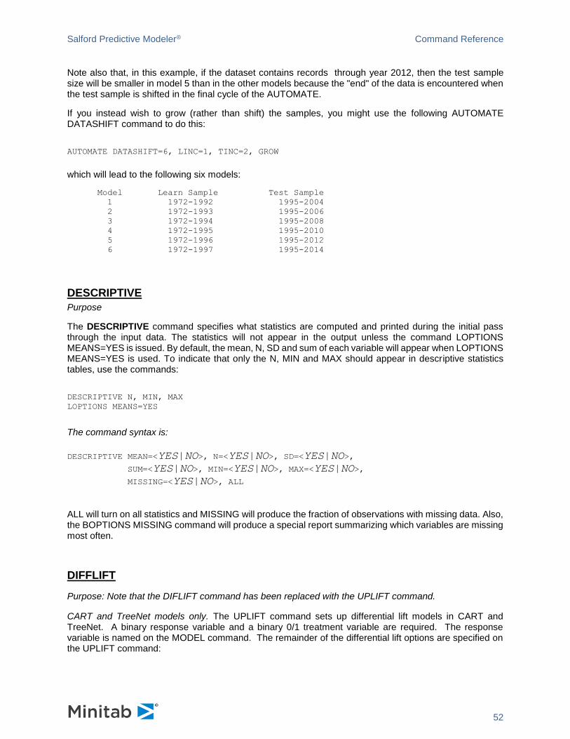
Salford Predictive Modeler® Command Reference
52
Note also that, in this example, if the dataset contains records through year 2012, then the test sample size will be smaller in model 5 than in the other models because the "end" of the data is encountered when the test sample is shifted in the final cycle of the AUTOMATE.
If you instead wish to grow (rather than shift) the samples, you might use the following AUTOMATE DATASHIFT command to do this:
AUTOMATE DATASHIFT=6, LINC=1, TINC=2, GROW
which will lead to the following six models:
Model Learn Sample Test Sample
1 1972-1992 1995-2004
2 1972-1993 1995-2006
3 1972-1994 1995-2008
4 1972-1995 1995-2010
5 1972-1996 1995-2012
6 1972-1997 1995-2014
DESCRIPTIVE
Purpose
The DESCRIPTIVE command specifies what statistics are computed and printed during the initial pass through the input data. The statistics will not appear in the output unless the command LOPTIONS MEANS=YES is issued. By default, the mean, N, SD and sum of each variable will appear when LOPTIONS MEANS=YES is used. To indicate that only the N, MIN and MAX should appear in descriptive statistics tables, use the commands:
DESCRIPTIVE N, MIN, MAX
LOPTIONS MEANS=YES
The command syntax is:
DESCRIPTIVE MEAN=<YES|NO>, N=<YES|NO>, SD=<YES|NO>,
SUM=<YES|NO>, MIN=<YES|NO>, MAX=<YES|NO>,
MISSING=<YES|NO>, ALL
ALL will turn on all statistics and MISSING will produce the fraction of observations with missing data. Also, the BOPTIONS MISSING command will produce a special report summarizing which variables are missing most often.
DIFFLIFT
Purpose: Note that the DIFLIFT command has been replaced with the UPLIFT command.
CART and TreeNet models only. The UPLIFT command sets up differential lift models in CART and TreeNet. A binary response variable and a binary 0/1 treatment variable are required. The response variable is named on the MODEL command. The remainder of the differential lift options are specified on the UPLIFT command:
Salford Predictive Modeler® Command Reference
53
MODEL <response_var>
CATEGORY <response_var>
UPLIFT TREATMENT=<treatment_var>, WEIGHT=<RESPONSE|TREATMENT|CROSS|QUAD>
CART GO (or TREENET GO)
<response_var> must be binary and declared as categorical
<treatment_var> must be binary and coded as 0/1
WEIGHT indicates one of four different weighting schemes:
RESPONSE: weights are modified such that the weighted sum of records for the responder group equals the weighted sum of records for the non-responder group
TREATMENT: weights are modified such that the weighted sum of records for the treated group equals the weighted sum of records for the untreated group. Unless specified this is the default
CROSS: weights are modified such that both WEIGHT=RESPONSE and WEIGHT=TREATMENT conditions are met
QUAD: weights are modified such that the weighted sum of records for each of the four {RESPONSE by TREATMENT} combinations are equalized
CART differential lift models have one further option:
DIFFLIFT TARGET=<NATURAL|XOR>
The default is XOR. NATURAL will use the original binary target variable rather than the "xor" synthetic target normally used, but the node-specific weights (shares) will still be based on the WEIGHT option.
DISALLOW
Purpose
CART only. The DISALLOW command specifies how predictor variables are constrained to be used, as primary splitters and/or as surrogates, at various depths of the tree and according to the node learn sample size.
By default, all predictors are allowed to be used as primary splitters (i.e., competitors) and as surrogates at all depths and node sizes. For each predictor, the DISALLOW command is used to specify at which depths and in which partitions (by size) the predictor is NOT permitted to be used, either as a splitter, a surrogate, or both. The command syntax is:
DISALLOW <variable> [ , <variable>,... /
ABOVE=<depth>, BELOW=<depth>,
MORE=<node_size>, FEWER=<node_size>,
SPLIT | SURROGATE ]
To enable a DISALLOW command to apply to all variables, use the syntax
DISALLOW * [ / ABOVE=<depth>, BELOW=<depth>,
MORE=<node_size>, FEWER=<node_size>,
SPLIT | SURROGATE ]
Salford Predictive Modeler® Command Reference
54
ABOVE, BELOW these options may be used together to describe the following depth ranges in which a variable is not used (D=depth):
ABOVE=N variable will not be used if depth D <= N, i.e., at depth N or shallower.
BELOW=M variable will not be used if depth D >= M, i.e., at depth M or deeper.
ABOVE=N, BELOW=M:
N=>M: this defines a depth range in which the variable will not be used, i.e., the variable will not be used if depth is between N and M, inclusive.
N<M: this defines two depth ranges in which the variable will not be used. The variable will not be used if D <= N (depth N and shallower) or if D => M (depth M and deeper).
MORE, FEWER: similarly, the MORE and FEWER options operate on the node size (number of learn sample observations in the node being split, before any subsampling is done) rather than the depth:
MORE=N: variable will not be used if the node has N or more records.
FEWER=M: variable will not be used if the node has M or fewer records.
MORE and FEWER may be issued together to form a joint condition.
The DISALLOW command is cumulative. To reset all DISALLOW specifications (i.e., to return to the default), issue the empty command:
DISALLOW
Variable groups may be used in the DISALLOW command similarly to variable names.
DISCRETE
Purpose
The DISCRETE command sets options specific to discrete or categorical variables. The command syntax is:
DISCRETE [ TABLES = NONE | SIMPLE | DETAILED ,
CASE = MIXED | UPPER | LOWER ,
MISSING = MISSING | LEGAL | TARGET | ALL ,
REFERENCE = FIRST | LAST ,
MAX = <n, n>, ORDER = <YES|NO>, FP = NO | WARN | LEARN | TEST | BOTH,
ALLLEVELS = <YES|NO> ]
TABLES controls whether frequency tables should be printed following data preprocessing. SIMPLE generates a listing of the levels encountered for each discrete variable and total counts (across learn and test samples). DETAILED breaks down counts by learn and test sample, and also by the dependent variable for classification trees. The default is SIMPLE.
Salford Predictive Modeler® Command Reference
55
CASE controls whether character strings are case-converted. The default is MIXED.
MISSING controls whether missing values for discrete variables are treated as truly MISSING or are considered a legal and distinct level. LEGAL will process missing values for nontarget variables as legal. TARGET will process missing values for a model target only as legal. ALL will process missing values for all variables as legal.
REFERENCE specifies which level is considered the reference, or "left out", level when forming "dummy variables" in REGRESS, GPS, and LOGIT. By default, the FIRST level based on alphanumeric ordering is considered the reference level. You may wish to change this to the LAST level to reach agreement with some other software that uses a different coding convention.
MAX MAX specifies the maximum number of distinct levels in discrete variables. The default is 20000,60000, which permits up to 20000 distinct classes for numeric variables and up to 60000 for character variables. You should only consider increasing this parameter if the program is unable to obtain a complete tabulation of one or more of your discrete variables. Both values must be at least 100, exceptif you want the number of distinct values to be unlimited in which case use a value of 0, e.g., DISCRETE MAX=0,0.
Note: it may happen that a variable has too many distinct values to tabulate completely. This is most likely to occur with character variables, especially those with long string values. Also, this may be due to treating an ordinal variable as discrete (categorical). DISCRETE MAX=<n,n> can be used to increase resource allocation for tabulating discrete variables which may allow a full tabulation to take place. DISCRETE MAX=AUTO,AUTO allows the tables to grow without bound, however, in extreme cases this may impede performance if too many distinct data values are processed.
ALLLEVELS By default, node statistics will not list discrete variable levels for a node that is not represented (N=0) in that node. Specifying ALLLEVELS=YES results in a complete tabulation of levels including those with N=0 in the node.
ORDER Discrete variable splitters and cross validation for classification trees can be affected by the sorting of your dataset. ORDER=YES adjusts for any sorting in your data and should be used when comparing results with previous versions.
FP controls whether out-of-sample levels are reset to missing. An out-of-sample level is one that appears in one of the two data samples (learn, test) but not the other. Such levels can lead to structural modeling problems. The default is FP=TEST, which resets any levels found in the test sample that are not also found in the learn sample to missing.
The default is
DISCRETE TABLES=SIMPLE, CASE=MIXED, MISSING=MISSING,
REFERENCE=FIRST, ALLLEVELS=NO, FP=TEST, ORDER=NO
Salford Predictive Modeler® Command Reference
56
ECHO
Purpose
The ECHO Command suppresses results streamed to the classic output window (GUI) or console (non-GUI). It does not affect results streamed to an output file or saved dataset. The command syntax is:
ECHO ON|OFF
The default is:
ECHO ON
ERROR
Purpose
Note: the ERROR command is deprecated in favor of the PARTITION command.
The ERROR command is now deprecated in favor of the PARTITION command. The ERROR command remains to support older command scripts.
ESTIMATE
Purpose
The ESTIMATE command is now deprecated in favor of the MARS GO command. The ESTIMATE command remains to support older command scripts.
EVAL
Purpose
The EVAL evaluates one variable against one or more scores. The command syntax is:
EVAL <target>, <score>, [ <score>, .... / BINS=<n>,
SCORETYPE=<PROB|LOGIT|RAW> ]
If the target is a multinomial variable, you may indicate a focus class with the FOCUS command. Results can be computed separately by a STRATA variable. For example:
CATEGORY CHOICE
FOCUS CHOICE=4
STRATA REGION
EVAL CHOICE, RESPONSE1, RESPONSE2 / BINS=50
By default, the scores will be assumed to be probabilities in the range [0, 1]. However, if they should be treated as logistic model scores and transformed when appropriate to probabilities, use the SCORETYPE=LOGIT option. If they are neither logistic scores nor probabilities, use the SCORETYPE=RAW option, in which case scores will be used to rank order the data for ROC and K-S statistics but some classification reporting will be unavailable.
Salford Predictive Modeler® Command Reference
57
EXCLUDE
Purpose
The EXCLUDE command specifies a list of independent variables to exclude from the analysis. The command syntax is:
EXCLUDE <varlist>
in which <varlist> is a list of variables NOT to be used in the model building process. All other variables will
be used.
The EXCLUDE command specifies variables that should not be used as predictors in the model. In other words, all variables other than the target and those listed in EXCLUDE and WEIGHT commands will be used as predictors. For example:
EXCLUDE DENSITY, AGE, INCOME, REGION$, IQ, GENDER$
EXCLUDE can modify an existing KEEP list by using the /KEEP option. Suppose a lengthy KEEP list is already in use, and you wish to simply exclude two of the variables rather than restate the entire lengthy list. The following provides an example of how to accomplish this:
KEEP AGE,IQ,REGION,INCOME,...
EXCLUDE IQ,REGION / KEEP
EXIT
Purpose
The EXIT command. The command syntax is:
EXIT
Note: the EXIT command is a synonym of the QUIT command.
FOCUS
Purpose
CART only. The FOCUS command specifies which class is treated as the focus or response class for a categorical variable. This influences some statistical measures as well as the sign of regression coefficients since the choice of the focus class has a bearing on how the model is expressed or parameterized for Logit, and GPS. Its syntax is:
FOCUS <variable1>=<class1> [, <variable2>=<class2>, ... ]
For example:
FOCUS RESPONSED$="YES"
FOCUS REGION="Calif", OUTCOME=1, GENDER=0
Salford Predictive Modeler® Command Reference
58
Unless otherwise specified on the FOCUS command, the focus class for a categorical variable is the class that alphanumerically sorts first, except for variables that take on values -1/1 or 0/1 in which case the 1 class is treated as the focus class.
FORCE
Purpose
CART only. The FORCE command identifies CART splits to be created in a CART tree, in lieu of the splits that CART would naturally determine based on the learn data. The command syntax is:
FORCE node [ SURROGATE=<n>, SENSE=<SAME|REVERSED>, ] ON <predictor> AT <splits>
in which <node> is either ROOT or a phrase that describes the node position in terms of its left-right branching from the root. Some examples are:
FORCE ROOT ...
FORCE LR ... (right daughter of the left daughter of the root node) FORCE RRRLR ...
Surrogate splits can be specified with the SURROGATE= option, otherwise the split will be implemented at the primary split at a given node. If the "sense" of the surrogate split is to be reversed relative to the primary split, use the SENSE=REVERSE option, otherwise the same sense is assumed. For example:
FORCE ROOT ON GENDER$ AT "Male", "Unknown"
FORCE LLRL SURROGATE=1 ON REGION SENSE=REVERSED AT 0,3,4,7,999
FORCE R ON INCOME AT 100000
By default, the tree is permitted to grow "beyond" those nodes that are forced. For example, you might FORCE only the root node split in which case the branches of the tree are free to grow once the root has been forced. However, to request a "strict" interpretation of FORCE commands, so that only forced nodes are created and no branch is grown beyond the FORCE criteria, issue the FORCE EXACT=YES along with your other FORCE commands:
FORCE EXACT=YES
The default is FORCE EXACT=NO.
To reset forced splits, use the command with no options
FORCE

Salford Predictive Modeler® Command Reference
59
FORMAT
Purpose
The FORMAT command controls the number of digits that are displayed to the right of the decimal point in analysis output. You may select from 1 to 9 digits, or 0 digits, or -1 for no digits and no decimal point. The default is 5.
The UNDERFLOW option prints tiny numbers (those that would appear to be zero in the chosen precision) in scientific (exponential) notation. The command syntax is:
FORMAT <#> [/UNDERFLOW]
Examples:
FORMAT=5
FORMAT=0
FORMAT=9/UNDERFLOW (print tiny numbers with exponents)
FPATH
Purpose
The FPATH command lets you specify an automatic path prefix for file names. Use it to read a file from or to direct output to a specific directory or device. There are six types of files for which you can specify prefixes individually.
OUTPUT text output (.DAT) files in OUTPUT commands.
SAVE output datasets (all formats, e.g., .CSV, .XLS).
SUBMIT command script (.CMD) files.
GROVE model files (.GRV) files.
USE input datasets (all formats, e.g., .CSV, .XLS)
TRANSLATE text files created by TRANSLATE command.
You can specify the same prefix for multiple file types; that is, you can store many different file types in the same directory. The command syntax is:
FPATH 'prefix' / [ OUTPUT SAVE SUBMIT GROVE USE TRANSLATE ]
Examples:
FPATH 'D:' / SAVE (direct all output data files to device D:)
FPATH '\MSETS\' / USE GROVE SAVE (datasets and grove files to \MSETS)
FPATH 'C:\USR\STATS\' / SUBMIT (.CMD files in directory on drive C:)
Salford Predictive Modeler® Command Reference
60
GPS Pathseeker Regression
Purpose
The GPS command builds regression and classification models using the GPS/Generalized Lasso algorithm. All options on the GPS command are optional. The command syntax is:
GPS [ GO,
ELASTICITY=<x>
LASSO, RIDGE, COMPACT,
ELIST=(<x1>,<x2>,...),
OPTIMAL=<DEFAULT|AVGLL|CLASS|ROC|LIFT|MSE|MAD|MAPE>,
START=<x>, END=<x>, INTERVALS=<n>, ORIGIN=<MAXIMAL|OPTIMAL>,
LISTWISE=<YES|NO>, BALPHA=<x>, ALGORITHM=<COVARIANCE|NAIVE>,
PREDICTORS=<N>, BOOTSTRAP=<N>, ROCSEQUENCE=<YES|NO>,
LEARNRATE=<x>, SPEED=<N>, STANDARDIZE=<YES|NO>, STEPS=<N>,
UNREGULARIZED=<YES|NO>, LOSS=<LS|LAD>, POINTS=<N>, EVAL=<x>,
SEQUENCE=<FULL|BRIEF|NO>, MAXCORR=<x>, QUANTILE=<x>,
BINARY=<CORR|PROB|MISCLASS>, SEARCH=<YES|NO> ]
To build the model, include the GO option in your GPS command:
GPS ... GO ...
ALGORITHM chooses between "covariance updating" and naive algorithms. The default is covariance updating.
BALPHA specifies the alpha-significance for computing upper and lower confidence bounds on coefficients when bootstrapping. The default is 0.05.
BINARY chooses between correlation criterion (~ 1-AUC), probability squared error loss and misclassification risk for logistic models. The default is correlation criterion.
BOOTSTRAP specifies the number of bootstrapping cycles to use on the learn sample to estimate upper and lower bounds on each coefficient. The default is 0, which suppresses bootstrapping.
LASSO chooses the lasso model (elasticity = 1.0).
RIDGE chooses the ridge model (elasticity = 2.0).
COMPACT chooses the compact model (elasticity = 0.0).
ELASTICITY selects the "elasticity" between 0.0 and 2.0. 0.0 is stepwise, 1.0 is lasso and 2.0 is ridge. The default is 0.0 (Compact), 1.0 (Lasso), 1.1 (Ridged Lasso) and 2.0 (Ridge).
ELIST selects a series of elasticities, up to 100.
START beginning elasticity value, between 0.0 and 2.0.
END ending elasticity value, between 0.0 and 2.0.
INTERVALS number of equally spaced points including (start, end). Up to 100 intervals are allowed.
EVAL path evaluation point control: larger values concentrate more points towards the end of the path (regularized models only). EVAL must be greater than zero, and the default value is 1.0.
LEARNRATE sets the step size scale factor, which is the maximum fractional reduction of risk allowed at each step. The default is 0.001.
Salford Predictive Modeler® Command Reference
61
LISTWISE uses listwise deletion of records to handle missing data. Without this, missing data are imputed to mean values. The default is LISTWISE=YES.
LOSS chooses between least absolute deviation and squared error loss for regression models. The default is squared error.
MAXCORR Limits entry of new predictors into model to those with correlation with existing models below a threshold. Sensible values to test are 0.5, 0.6, 0.7, 0.8, 0.9, 0.95, 0.99.
ORIGINAL for TreeNet models that feed into GPS, such as ISLE and RuleLearner® models, ORIGIN specifies whether the process should focus on the optimal number of trees or the maximal number of trees.
OPTIMAL specifies which optimality criterion is to be used to search for the single optimal model. DEFAULT will result in ROC being used for binary models and MSE for regression models. If SEARCH=NO, this option has no effect.
POINTS sets the number of path points to be evaluated, for regularized only. The default is 200.
PREDICTORS When GPS begins it scans and evaluates ALL predictors to add the first variable to the model. It repeats this process until it has selected the number of variables specified by PREDICTORS. Once this limit is reached the model may be further refined through coefficient adjustment but no new variables may enter the model. The default value PREDICTORS=0 sets no limit allowing GPS to always consider adding a new predictor at any stage of model development. Setting PREDICTORS= is essential when working with potentially thousands or hundreds of thousands of predictors. In such cases we recommend values such as PREDICTORS=500. Experimentation with several different values is always good practice.
QUANTILE Input predictor variable conditioning: This provides robustness to outliers among the predictor variables. Each predictor value x(i,j) is replaced by max(low(j),min(high(j),x(i,j))) where low(j) = q'th_quantile{x(i,j),i=1,nobs} and high(j) is the corresponding (1-q)'th quantile. A value of 0.0 produces no conditioning.
ROCSEQUENCE controls whether ROC, lift and gains charts are computed for each point on each elasticity path for logistic models. The default is ROCSEQUENCE=YES. NO can speed up the model evaluation stage of a GPS run, but ROC, lift and gains charts will then be unavailable.
SEARCH determines whether test or CV performance measures are considered for all points on each path in order to identify the optimal model. If SEARCH=YES, then the OPTIMAL option selects the particular criterion that is used.
SEQUENCE produces an error rate sequence for regression models.
SPEED sets the speed/exactness trade-off parameter. Increasing this value increases speed by the same factor, possibly decreasing exactness. The slowest value is 1, which stays closest to the exact path. The default is 1.
STANDARDIZE will scale the predictor data by the learn sample standard deviation. The default is YES for straightforward GPS regression and logistic regression. The default is NO for the ISLE and RuleLearner® two stage models using only trees or nodes as predictors. Not standardizing will favor the inclusion of predictors with larger learn sample variances and standardizing can influence model details and performance substantially. If in doubt run your model both ways and select the better performing strategy. The model results are always presented relative to the original data values.
STEPS sets the maximum number of steps. The default is 5000.

Salford Predictive Modeler® Command Reference
62
UNREGULARIZED uses unregularized regression to select the solution. The default is UNREGULARIZED=NO.
For modeling TreeNet-based ISLE or RuleLearner models, the following additional options are available:
GPS [ SAVE="<filename>", SAVEONLY=<BOTH|ISLE|RULELEARNER>, NRULES=<n>,
RULELEARNER=<yes|no>, ISLE=<yes|no>, HRULELEARNER=<yes|no>,
HISLE=<yes|no>, TREES=<yes|no>, VARS=<yes|no>,
BLEND=<yes|no>, ALL=<yes|no> ]
SAVE names a dataset that will contain the RuleLearner dummies, ISLE scores, original predictors, IDVAR variables, target and learn/test indicator.
SAVEONLY allows you to request that only, for instance, ISLE scores be included in the SAVEd dataset, which can reduce the size of the dataset considerably.
NRULES limits the number of RuleLearner rules reported. The default is 10.
RULELEARNER models the target on node dummies.
HRULELEARNER models the target on node dummies plus original predictors.
ISLE models the target on individual tree responses.
HISLE models the target on individual tree responses plus original predictors.
TREES models the target on tree responses and node dummies.
VARS models the target on just the original predictors.
BLEND models the target on node dummies, tree scores and original predictors.
ALL builds all models (RULELEARNER/HRULELEARNER, ISLE/HISLE, TREES, VARS, BLEND).
When run as the second stage in a pipeline model (e.g., ISLE, RULELEARNER) GPS requires an explicit test sample or cross validation. If PARTITION NONE is in effect, GPS will use 5-fold cross validation. The defaults are:
GPS ELIST=(0,1,1.1,2), LOSS=LS, STEPS=5000, SPEED=1,
LEARNRATE=0.001, POINTS=200, PREDICTORS=0, EVAL=1.0,
BALPHA=0.05, MAXCORR=1.0, BINARY=CORR, NRULES=10,
QUANTILE=0.0, SEQUENCE=FULL, ORIGIN=OPTIMAL,
OPTIMAL=DEFAULT, ALGORITHM=COVARIANCE, LISTWISE=YES,
BOOTSTRAP=0, STANDARDIZE=YES, UNREGULARIZED=NO, SEARCH=NO
Salford Predictive Modeler® Command Reference
63
GROUP
Purpose
The GROUP ommand is a synonym for the VARGROUP command. The command syntax is:
VARGROUP <groupname> = <variable>, <variable>, ...
Group names are used like variable names in commands that process variable lists, resulting in more compact lists. The following commands set up three groups and use them in the KEEP, AUXILIARY, CATEGORY and CLASS commands (along with variables SEGMENT, AGE, PROFIT) for a three-level classification tree:
VARGROUP DEMOGRAPHICS = GENDER RACE$ REGION$ PARTY EDUCLEV
VARGROUP CREDITINFO = FICO1 FICO2 TRW LOANAMOUNT AUTOPAYMENT,
MORTGAGEAMOUNT MORTGAGEPAY
VARGROUP CREDITRANK = RANKVER1 RANKVER2 RANKVER3
CATEGORY DEMOGRAPHICS TARGET$ SEGMENT CREDITRANK
CLASS CREDITRANK 0="Not available", 1="Poor", 2="Good",
3="Excellent"
AUXILIARY AGE PROFIT CREDITINFO PROFIT
MODEL TARGET$
KEEP DEMOGRAPHICS CREDITINFO SEGMENT CREDITRANK
CART GO
Groups can contain a mix of character and numeric variables; however, the CLASS command will accept homogenous (all character or all numeric) groups only. A variable may be included in more than one group. If a group is assigned a name that is identical to a variable name, the group name will take precedence in variable lists (i.e., the variable name will be masked).
The following commands recognize variable groups:
CATEGORY, KEEP, EXCLUDE, AUXILIARY, IDVAR, DISALLOW
STATS, PENALTY, CLASS, PLOT, HISTOGRAM, ICL
GROVE
Purpose
The GROVE command names a grove file in which to store the next model (or ensemble of model) or to use in the next TRANSLATE or SCORE operation. Its syntax is:
GROVE <filename>
For example:
MODEL TARGET
KEEP PREDICTOR
PARTITION TEST=.2
GROVE "c:\modeling\rev1\groves\M_2b.grv"
CART GO
or
Salford Predictive Modeler® Command Reference
64
GROVE "\\drive\archives\model341.grv"
TRANSLATE LANGUAGE=C OUTPUT="implementation.c"
To convert a legacy "treefile" (e.g., mytree.tr1) from a previous version of CART to a grove, use the IMPORT option, e.g.:
GROVE "\robustus\projects\groves\J3b.grv" IMPORT="c:\c3po\legacy.tr1"
To skip loading auxiliary variable counts, which can require considerable memory in large CART trees, use the NOAUXCOUNTS option:
GROVE "file.grv" NOAUXCOUNTS
To restore the SPM model setup from a previous session, use the SESSION option, for example:
USE "\dataset\analsys.xls"
GROVE "model0528.grv" SESSION
CART GO
HARVEST
Purpose
The HARVEST command specifies which models in a grove are processed (during SCORE or TRANSLATE) and how those models are pruned for processing.
To select models in a grove, the HARVEST SELECT command is used:
HARVEST [ ENGINE=<CART|TN|RF|MARS|GPS|REGRESS|LOGIT|PROBIT>, ]
SELECT [ ALL | RELERR=<x> | COMPLEXITY=<x> | NODES=<n> |
RANDOM=<n> | KEEP=<n1,n2,...> | EXCLUDE=<n1,n2,...> |
DEPTH=<n>]
If the HARVEST SELECT command is not issued, all models in the grove are selected. To select all models of a given type, simply use the HARVEST ENGINE SELECT option, e.g.,
HARVEST ENGINE=CART SELECT
Prior to being used in a scoring or translation step, the selected models are pruned to their optimal size. To specify a pruning condition to be applied to all of the selected models, use the HARVEST PRUNE command:
HARVEST PRUNE [ NODES=<n> | DEPTH=<n> | RELERR=<x> |
TREENUMBER=<n> | COMPLEXITY=<x> |
BASIS=<n> | NTREES=<n> ]
If there are several models selected, you may list different pruning criteria for each with the HARVEST PRUNE LIST command:
HARVEST PRUNE LIST [ NODES=<n1,n2,...> | DEPTH=<n1,n2,...> |
TREENUMBER=<n1,n2,...> | BASIS=... |
NTREES=<n1,n2,...> ]
Salford Predictive Modeler® Command Reference
65
The options on the HARVEST SELECT command are:
ALL select all trees in the grove
KEEP, EXCLUDE selects (or excludes) individual models according to their position in the grove, for instance:
HARVEST ENGINE=TREENET SELECT KEEP=2,3,7
HARVEST ENGINE=CART SELECT EXCLUDE=5,6
RELERR=<x> select all trees which, when pruned to optimal size, have test sample relative error rate (or resubstitution error rate if no test sample was used) less than <x>.
COMPLEXITY=<x> select all trees which, when pruned to optimal size, have complexity threshold less than <x>.
NODES=<n> select all trees which, when pruned to optimal size, have less than or equal to <n> terminal nodes.
RANDOM=<n> randomly select up to <n> trees from the grove
DEPTH=<n> select all trees which, when pruned to optimal size, are less than or equal to <n> nodes deep.
HARVEST CVTREES=YES|NO specifies whether ancillary trees created as part of a CART cross validation model are selected. By default they are not.
A new grove file, containing only the harvested trees, may be created with the OUTPUT option, for example:
HARVEST SELECT KEEP=5 OUTPUT="justone.grv"
For scoring or translating CART classification trees using the test sample (rather than learn sample) class probabilities, use the command
HARVEST PROBS=TEST
This option is ignored if the model was built without a test sample or for model types other than CART.
TreeNet-GPS pipeline models, such as ISLE and RuleLearner, are scored in their optimal form by default. If you wish to select a different elasticity path and point, use the syntax:
HARVEST PIPELINE [MODE] [ELASTICITY=<x>, POINT=<n>]
where the mode is BASELINE, ISLE, RULELEARNER, HISLE, HRULELEARNER, TREES, VARS or BLEND. For example, if your grove contains both ISLE and RuleLearner models, you may wish to score each of them at specific points along with the baseline TreeNet model:
HARVEST PIPELINE BASELINE
HARVEST PIPELINE ISLE, ELASTICITY=1.1, POINT=130
HARVEST PIPELINE RULELEARNER, ELASTICITY=2, POINT=307
Salford Predictive Modeler® Command Reference
66
HELP
Purpose
The HELP command The command syntax is:
HELP [<command>]
HELP with no arguments will give a command listing.
Examples:
HELP (succinct listing of all commands)
HELP KEEP (details about the KEEP command)
HELP AUTOMATE DRAW (details about one of the AUTOMATE commands)
HELP AUTOMATE (details about all AUTOMATE commands, quite a few!)
HELP _ALL_ (details about all commands)
Note for GUI users
The Help menu provides comprehensive on-line information concerning SPM menus, commands, BASIC programming, and frequently-asked questions.
HISTOGRAM
Purpose
The HISTOGRAM command The command syntax is:
HISTOGRAM <var1> [, <var2> , <var3> , ... , / FULL, TICKS | GRID, WEIGHTED, NORMALIZED, BIG ]
The console plot (low-resolution, non-GUI) is normally a half screen high: the FULL and BIG options will increase it to a full screen (24 lines) or a full page (60 lines).
TICKS and GRID add two kinds of horizontal and vertical grids.
WEIGHTED requests plots weighted by the WEIGHT command variable.
NORMALIZED scales the vertical axis to 0 to 1 (or -1 to 1).
Examples:
HISTOGRAM IQ / FULL, GRID
HISTOGRAM LEVEL(4-7) / NORMALIZED
Only numerical variables may be specified.
Variable groups may be used in the HISTOGRAM command similarly to variable names.
Salford Predictive Modeler® Command Reference
67
HOTSPOT
Purpose
The HOTSPOT command reports association rules (“hotspots”) for CART models built using AUTOMATE PRIORS. Its syntax is report association rules (“hotspots”) for CART models built using AUTOMATE PRIORS. Its syntax is
HOTSPOT [ GO, N=<n>, NRULES=<n>, NODES=<NONTERMINAL|TERMINAL|ALL>,
RICHNESS=<MEANRATIO|SUMRATIO|MEAN|SUM> ]
N limits the report to the top N richest hotspots (nodes).
NRULES reports the rules only for the top NRULES hotspots
NODES governs which types of nodes are considered
RICHNESS determines how the node richness is defined for continuous targets,
The default is:
HOTSPOT N=100, NRULES=100, NODES=ALL, RICHNESS=MEANRATIO
ICL
Purpose
TreeNet only. The ICL command defines interaction control lists in TreeNet. It is more fully explained in its own chapter "TreeNet Interactive Control Language Commands". ICL command(s) gives you complete control over structural interactions allowed or not allowed during model building. A structural interaction means that a group of variables enters jointly along at least one branch somewhere in a tree sequence. ICL commands enforce additional restrictions on the list of candidate predictors considered by the engine at each node during model building.
The command syntax is:
ICL ADDITIVE=<varlist>
ICL ALLOW=<varlist> [ / <n> ]
ICL DISALLOW=<varlist> [ / <n> ]
ICL N2WAY=<N>, PENALTY=<x>
N2WAY limits on the number of two-way interactions to report, defaults to 5.
PENALTY must be 0.0 <= x <= 1.0, and defaults to 0.0. PENALTY inhibits TreeNet from introducing new variables (and thus interactions) within a branch of a tree. The default of 0.0 allows free use of the best splitter anywhere. A value of .05 would require any new variable to be more than 5% better than any variable already used along the branch in question.
ADDITIVE specifies predictors that are to be treated as additive-only (no interactions) in the model. For example, when TreeNet creates a tree, if the root node splitter is additive only then it will be the only predictor considered as a splitter in the remainder of that tree.
ALLOW specifies predictor interactions that are allowed in the model
Salford Predictive Modeler® Command Reference
68
DISALLOW specifies predictor interactions that are not permitted in the model
The following rules control engine's behavior in terms of interactions:
1. No ICL commands (default) - all interactions are structurally allowed
2. Only ICL ADDITIVE commands - interactions are ALLOWED only among the variables NOT LISTED in the ADDITIVE commands
3. Only ICL ALLOW commands - interactions are ALLOWED only within the groups of variables LISTED in each ICL ALLOW command, all remaining variables (NOT LISTED) are NOT ALLOWED to interact
4. ICL ALLOW together with ICL DISALLOW commands - same as 3 above but NOT ALLOWING interactions among the variables LISTED in each DISALLOW group
Note: case 1 above (ICL empty) is equivalent to ICL ALLOW "all predictors" (case 3). All examples below assume KEEP X1 X2 X3 X4 X5: ICL or nothing
all interactions are allowed (rule 1) ICL ADDITIVE X1 X2
allows interactions only among {X3,X4,X5} (rule 2) ICL ALLOW X1 X2
ICL ALLOW X3 X4
allows interaction between {X1,X2}, between {X3,X4} but not between {X1,X3}, {X1,X4}, etc. X5 is additive (rule 3) ICL ALLOW X1 X2 X3 X4
ICL DISALLOW X3 X4
allows any interaction among {X1,X2,X3,X4} except between {X3,X4}. For example, {X1,X2,X4} can enter along a branch but {X1,X3,X4} can not (rule 4) ICL ALLOW X1 X2
ICL DISALLOW X1 X2
A quick way to DISABLE ALL interactions (rule 4) Finally note that the joint use of ADDITIVE and ALLOW/DISALLOW commands is possible but
discouraged because of ambiguous interpretation. N2WAY sets a limit on the number of two-way interactions to report and defaults to 5. PENALTY must be
0.0 <= x <= 1.0, and defaults to 0.0. PENALTY inhibits treenet from introducing new variables (and thus
interactions) within a branch of a tree. The default of 0.0 allows free use of the best splitter anywhere. A value of .05 would require any new variable to be more than 5% better than any variable already used along the branch in question. VARGROUPs can be used in lieu of the <varlist> specification in
the ADDITIVE, ALLOW and DISALLOW options.
ICL PENALTY=<p> where 0<=p<=1
imposes a penalty on introducing a new variable into a branch of the tree under construction. If X1 and X2 are already on a given branch then the penalty causes TreeNet to continue using these two variables to extend the branch.
ICL PENALTY is intended to inhibit interactions in general while the
DISALLOW commands prohibit interactions.

Salford Predictive Modeler® Command Reference
69
IDVAR
Purpose
The IDVAR command lists extra variables to save in the next dataset to be SAVED. These can be any variables from the USE dataset that are not in the model. (Model variables are saved with the SAVE / MODEL option.). The command syntax is:
If every case in your file has a unique identifier, say SSN, you could specify:
IDVAR SSN
SAVE “WATER.CSV”
The dataset WATER.CSV will include the variable SSN in addition to its normal contents.
If you want to include all the non-model and model variables in the saved dataset, you would issue:
IDVAR / ALL
SAVE <“filename”> / MODEL
Variable groups may be used in the IDVAR command similarly to variable names.
INTERACT
Purpose
MARS only. The INTERACT command specifies which variables are or are not allowed to interact in the model. The command syntax is:
INTERACT ALLOW | DISALLOW <variable1> [ * variable2 ]
Some examples are:
INTERACT ALLOW = _ALL_ / DISALLOW = GENDER, AGE
INTERACT DISALLOW = _ALL_ / ALLOW = VALUE * REGION,
SMOKER * AGE, CHECK
INTERACT DISALLOW = AGE, VALUE * NIGHT, VALUE * REGION
ISLE
Purpose
ISLE uses a combination of TreeNet trees and GPS generalized lasso models to perform model compression. The GUI Model Setup for the ISLE engine guides the process. From the command line, you must issue these commands in sequence:
GPS ISLE=YES
TREENET GPS=YES GO
Additional details are provided in the help entries for GPS and TreeNet.

Salford Predictive Modeler® Command Reference
70
KEEP
Purpose
The KEEP command The command syntax is:
KEEP <var1>, <var2>, .... [ / NOMISSING, MISSINGPCT=<x> ]
in which <var> is a predictor variable. If no list is specified, all variables are considered as predictors (unless
an EXCLUDE command is issued or a list of predictors is included on the MODEL statement).
Independent variables may be separated by spaces or commas.
Variables may also be separated by a hyphen, in which case they specify a range of variables based on the dataset positions. In this case, the variable preceding the hyphen should be positioned "earlier" in the dataset than the variable following the hyphen or an error message will result. For example:
KEEP AGE-IQ, FACTOR3-REGION$
KEEP X1-X534, X570-X600, GEOCODE_A-GEOCODE_Z
There are several shortcuts that can be used to specify certain types of variables:
KEEP _CHARACTER_ (all character variables)
KEEP _NUMERIC_ (all numeric variables)
KEEP _ISLE_ (all ISLE variables, e.g., TREE17)
KEEP _RULELEARNER_ (all RuleLearner variables, e.g., TREE_45_NODE_7)
For time-series data you can create lags by using the <> notation on the KEEP command. For instance, to include PARTY$ and its four lags as well as the fifth lag of INCOME and the second through fifth lag of INFLUENCE:
KEEP PARTY$<0-4>, INCOME<5>, INFLUENCE<2-5>,...
The lag notation only applies to predictors on the KEEP command; it does not extend to the EXCLUDE or MODEL commands. The KEEP command supports up to the 99999'th lag of a variable.
See the MODEL and EXCLUDE commands for other ways to restrict the list of candidate predictor variables.
To see the variables that are currently on the keep list, use:
KEEP / LIST, [ LONGFORM | SHORTFORM ]
LONGFORM will list variables individually, and is the default. SHORTFORM will list variables in groups using the dash convention if possible, resulting in a shorter list.
To have any predictors with missing values automatically filtered out of the modeling, use the NOMISSING option, e.g.,
KEEP / NOMISSING
KEEP X1-X5,X6<2>,AGE,GENDER / NOMISSING
To instead filter out predictors that have more than some threshold proportion of missing values, say, 30%, you could use the commands:

Salford Predictive Modeler® Command Reference
71
KEEP / MISSINGPCT=.30
KEEP X1-X5,X6<2>,AGE,GENDER / MISSINGPCT=.30
Lastly, to filter out predictors that have more than some threshold number (instances) of missing values, say, 10, you could use the commands:
KEEP / MISSINGN=10
KEEP X1-X5,X6<2>,AGE,GENDER / MISSINGN=10
The NOMISSING, MISSINGPCT and MISSINGN functionality is based on learn sample missing value prevalence.
A few commands can reference the keep list with the notation _KEEP_. The LCLIST, ICL and SVD commands allow you to use the term "_KEEP_" where you would ordinarily specify variables. For instance:
LCLIST _KEEP_ / ... (for linear combination list in CART)
ICL _KEEP_ / ... (for interaction control list in TreeNet)
SVD _KEEP_ / ... (for singular value decomposition)
KNOT
Purpose
MARS only. The KNOT command controls the number of degrees of freedom for (unrestricted) knot optimization in MARS models. The command syntax is:
KNOT FIXED=<X>
which will set the degrees of freedom in MARS models to <X>, a whole number greater than 0.0.
The KNOT command with no options will reset this option to the default, which is:
KNOT FIXED=3.0
Note: the options CROSS and TEST are no longer supported. Please contact the Salford Systems support team if you have questions.
LABEL
Purpose
The LABEL command The command syntax is:
LABEL <variable> = ”ADD LABEL IN QUOTES”
Examples:
LABEL RESPONSE="Did subject purchase at least one item? 1=yes, 0=no"
or
LABEL PARTY$="Political affiliation, sourced from public database."

Salford Predictive Modeler® Command Reference
72
If labels are embedded in your dataset (such as SAS(tm) datasets), they will be used in SPM and there is no need for you to issue LABEL commands unless you wish to change or remove them.
Variable groups may be used in the LABEL command similarly to variable names.
To see a summary of variable labels, issue the command:
LABEL _TABLE_
LCLIST
Purpose
CART only. The LCLIST command identifies a group of continuous predictors among which CART should attempt to produce a linear combinationis now deprecated in favor of LCLIST.The command syntax is: command syntax is:
LCLIST <varlist> [ / <options> ]
in which <varlist> can be an explicit list of continuous predictors or the _KEEP_ keyword (shorthand for whatever the keep list is for the model). Some examples:
LCLIST credit_score,rate,rebate
LCLIST _keep_
LCLIST x,y,z / N=100, EXH=YES
To reset all LCLISTs, simply issue the LCLIST command alone:
LCLIST
Multiple LCLIST commands can be issued. In this way, multiple linear combinations may be developed at each node. The linear combination with the highest improvement will be compared to the best univariate splitter in order to determine the primary splitter in the node.
The options are:
N=<n> specifies the minimum number of records required in a node for linear combination splits from this LCLIST to be considered. Smaller nodes will not consider this LCLIST. This is essentially an LCLIST-specific atom. Default=3.
W=<x> similar to N=<n> but based on sum of case weights. If this option is issued, a node must have a sum of case weights equal to or exceeding <x> for this LCLIST to be considered. This is essentially an LCLIST-specific weighted atom.
SIZE=<n> Must be > 1. The default is 6.
STORED=<n> Defines how many candidate linear combinations formed from the LCLIST are maintained in memory during the search. A high value allows for a more comprehensive search involving higher-ordered linear combinations, but at a potentially significant increase in compute time. Must be > 1. The default is 5.
OPTIM=<n> Must be 0 or greater. The default is 0.
PENALTY=<x> Must be in the range [0.5, 1.0] inclusive. Defaults to 0.9
Salford Predictive Modeler® Command Reference
73
POSITIVE=<yes|no> Specifies whether all coefficients must be constrained to be positive. The default is NO.
DELETE=<x> governs the backwards deletion of variables in the stepwise linear combination search algorithm. The default is 0.20.
DOF=<x> when comparing a linear combination against univariate competitors, the LC improvement is DOF-adjusted:
adj_imp = improvement * (N - X * (NC - 1) - 2) / (N - 2)
in which
N = number of records used in the LC search algorithm (usually the node size)
NC = number of nonzero coefficients in the LC improvement = unadjusted improvement, displayed in model results, reports, etc.
X = parameter specified on the DOF option.
For agreement with previous versions of CART (that used the LINEAR command), use DOF=1. To disable the adjustment, use DOF=0. The default is 1.0.
EXH=<yes|no> tells CART to repeat the stepwise search algorithm using each predictor in the LCLIST as the focal variable. This increases compute time proportional to the number of predictors in the LCLIST. It can, in some cases, yield better split points than the default approach. Default=NO.
SS=<yes|no> The default (SS=yes) allows the linear combination search algorithm to proceed even if some of the predictors in the have a high proportion of missing values or are constant. Disabling this feature (SS=no) causes CART to use a more stringent, listwise-like criterion for determine which records in a node are used in forming linear combinations and whether linear combination searching is even attempted in a node for this LCLIST.
SEARCH=<n> limits the linear combination search to only consider the topmost N univariate competitors in the LCLIST. The default is 10, the minimum value is 2. Smaller values reduce run time at the expense of perhaps not considering potentially valuable linear combinations.
LIMIT
Purpose
The LIMIT command allows tree growth limits to be set. The command syntax is:
LIMIT ATOM=<n|MINCHILDX3>, SUBSAMPLE=<n>, NODES=<n|AUTO>,
DEPTH=<n|AUTO>, LEARN=<n|AUTO>, TEST=<n|AUTO>,
DATASET=<n>, ERRORSET=<n>, LIST=<yes|no>,
MINCHILD=<n|LOG2>, WMINCHILD=<x>, WATOM=<x>
in which <n> is a whole number.
ATOM the smallest node that may be split in tree growing. The default is 10, however for RandomForests models we strongly recommend using a value of 2 to obtain the largest possible trees.
Salford Predictive Modeler® Command Reference
74
WATOM minimum weighted size for a node to be split. WATOM is only used if you explicitly set a nonzero value.
SUBSAMPLE node size above which a subsample is used to locate splits. CART only.
NODES forecast of the number of terminal nodes in the largest tree grown. Default of AUTO lets SPM set a value for you. Override allocates required workspace for unusual problems. CART only.
DEPTH limits maximal tree growth to a specified depth. Default of AUTO forecasts depth of largest tree likely to be grown.
LEARN maximum number of cases to allow into learning set. By default no limit is in effect other than that based on your license. AUTO removes current limit.
TEST maximum number of cases to allow into test set. By default no limit is in effect. AUTO removes current limit.
MINCHILD sets the minimum size for a child node. The default is 1.
WMINCHILD sets the minimum weighted size for a child node. It is only used if you explicitly set a nonzero value.
LIST lists the set of CART limitations currently in effect.
Some examples are:
LIMIT ATOM=15, NODES=150, LIST
LIMIT DEPTH=18
LIMIT LEARN=20000, TEST=5000
The defaults are:
LIMIT ATOM=10, WATOM=0, SUBSAMPLE=0, NODES=AUTO, DEPTH=AUTO,
LEARN=AUTO, TEST=AUTO, MINCHILD=1, WMINCHILD=0
On some platforms, CART can automatically determine the number of records in the USE= and ERROR FILE= datasets. But on other platforms CART cannot, and it will assume that there are 1000 records in these datasets. These assumptions may lead to poor choices of memory parameters if your datasets have considerably more records than 1000. In this case, use the DATASET and ERRORSET options to inform CART of the correct number of records in your datasets. Some examples are:
LIMIT DATASET=33000
LIMIT DATASET=100000, ERRORSET=75000
LINEAR
Purpose
CART only. The LINEAR command allows CART to search for linear combinations The LINEAR command is the simpler of two methods of computing linear combinations in CART; the LCLIST command offers a more powerful way of generating linear combination splits in CART.The command syntax is:
LINEAR [ N=<n1>, DELETE=<x>, LINSPLITS=<n2|AUTO>, EXHAUSTIVE ]
in which <x> is a fractional or whole number and <n1> and <n2> are whole numbers.
Salford Predictive Modeler® Command Reference
75
N specifies the minimum number of cases required in a node for linear combination splits to be considered. Smaller nodes will be split only on single variables.
DELETE governs the backwards deletion of variables in a stepwise algorithm. The default is 0.20.
LINSPLITS is a forecast of the maximum number of linear combination splits in the maximal tree. This value is estimated automatically by CART and normally need not be set. The automatic estimate may be overridden to allocate more linear combination workspace.
EXHAUSTIVE tells CART to attempt computing linear combinations using each continuous independent variable as the "perturbation" variable.
Linear combination splits are turned off by simply entering the command:
LINEAR
LOGIT
Purpose
The LOGIT command is used to toggle logistic model options, and to launch a binary or multinomial logistic model. The command syntax is:
LOGIT MEANS=YES|NO, QML=YES|NO, BHHH=YES|NO,
NEGWEIGHT=YES|NO, SDOUBLING=YES|NO, SHALVING=YES|NO,
LOG=YES|NO, TABLES=YES|NO, DELTA=YES|NO, FULL=YES|NO,
OVERFLOW=YES|NO, WHITE=YES|NO,
MODHESS=YES|NO, NESTING=YES|NO,
DERIVATIVE=YES|NO / AVERAGE | INDIVIDUAL | BOTH,
ELASTICITY=YES|NO / AVERAGE | INDIVIDUAL | BOTH,
PREDICTION_SUCCESS=YES|NO / NORMAL | CLASS | BOTH,
PLOTS = YES|NO / "<plot_character>", PROBIT=YES|NO,
CENTER=YES|NO, COVARIANCE=YES|NO, INTERCEPT=YES|NO,
PERFORMANCE=YES|NO
Numeric options are:
LOGIT CHANGE=<x>, NORM=<x>, GRADIENT=<x>, GHG=<x>, CONDITION=<x>,
SIGNIFICANCE=<x>, ITERATIONS=<n>, HALVINGS=<n>,
SECYCLE=<x>, SCENES=<x>, MAXCLASSES=<n>
To launch a logistic model, include the GO option on your LOGIT command:
LOGIT ... GO
NOTE: When toggling an option on, the '=YES' portion is not generally not needed. For example, the following two statements are equivalent:
LOPTIONS MEANS=YES DERIVATIVE=YES/BOTH PRED=YES/CLASS LOG=NO

Salford Predictive Modeler® Command Reference
76
LOPTIONS MEANS DERIVATIVE/BOTH PRED/CLASS LOG=NO
LOGIT control option details are as follows:
The MEANS option controls the printing of covariate means after the first pass through the data. The
QML option specifies that the Quasi-Maximum Likelihood covariance matrix is to be calculated following successful estimation of the model.
The WHITE option is used to specify White's grouped QML covariance matrix, in conjunction with an id variable (IDVAR command). If either QML covariance matrix is calculated, it will be used during subsequent hypothesis testing, and will affect t-values for estimated parameters.
BHHH controls the use of a BHHH approximation to the Hessian matrix during estimation.
NEGWEIGHT allows the use of negative case weights, which would normally be interpreted as missing values.
SDOUBLING and SHALVING enable step size doubling and halving during estimation.
LOG produces a detailed log during estimation, listing the parameter, change and gradient vectors, and the Hessian and covariance matrices after each iteration.
TABLES will turn off the printing of voluminous tabular output in some modules.
The DELTA option specifies that the DELTA method, rather than a first order approximation, is used to determine the variance of probability quantities.
The DERIVATIVE and ELASTICITY options control the printing of parameter derivatives and elasticities, based on an AVERAGE covariate vector or determined for each INDIVIDUAL case and then averaged.
PREDICTION requests the computation of the prediction success table, an accumulation of predicted probabilities by actual choice -- accumulation is NORMALLY over actual probabilities, although it can be based on probability vectors rounded into CLASSES such that only one element in the vector is equal to one while all other are zero.
The PLOTS option toggles certain plotting features, and allows the specification of default plotting character.
FULL specifies that the entire means, derivative and elasticity matrices should be computed, rather than just the "own" effects -- this will increase output and memory requirements in large conditional or mixed models.
OVERFLOW allows control of exponentiation overflows when computing elements of the logistic probability vector for the following operations: deciles of risk, prediction success, saving of residuals, derivative tables, elasticity tables. OVERFLOW=YES will correct overflows with the resulting probability set to 1.0, while OVERFLOW=NO will abort the process with an error message.
The CENTER option, when used for a by-choice conditional model, will cut the size of the temporary disk file in half.
COVARIANCE prints out hessian, covariance and correlation matrices their associated Eigen systems.
The INTERCEPT option controls whether an intercept (constant) is present.
The PROBIT option will, for binary poly models, add a PROBIT model after the LOGIT model is completed.
PERFORMANCE=NO suppresses the computation of logistic model performance measures such as integrated ROC, gains charts, etc.
Salford Predictive Modeler® Command Reference
77
CHANGE sets a maximum value for relative coefficient changes.
NORM sets a maximum value for the Euclidean norm of the relative change vector.
GRADIENT sets a maximum value for gradient elements.
CONDITION sets a maximum value for the hessian matrix condition before a singularity is assumed.
SIGNIFICANCE sets the significance level for multipliers in confidence interval construction (upper and lower bounds); for example, a significance level of 0.05 will result in a normal multiplier of 1.9600 (assuming the command LOPTIONS NORMAL is in effect).
ITERATIONS set a maximum on the number of iterations permitted per model.
GHG sets a maximum value for the gradient*hessian-inverse*gradient statistic.
MAXCLASSES is the maximum number of target classes allowed. The default is 20. If you wish to estimate a logistic model with more than 20 classes increase the MAXCLASSES setting appropriately.
The default values are:
LOGIT PLOTS, TABLES, NORMAL, OVERFLOW, CHANGE=.001,
NORM=.001, GRADIENT=., GHG=.0001, SIGNIFICANCE=.05,
CONDITION=1E-12, ITERATIONS=15, HALVINGS=15, SECYCLE=0,
MAXCLASSES=20, INTERCEPT
Successive LOGIT statements may be used -- they are cumulative up until the GO option is issued, at which point the model is built. For example:
LOGIT LOG MEANS=NO DERIVATIVES=NO
LOGIT GO
LOGIT LOG=NO MEANS DERIVATIVES/BOTH ELASTICITY/INDIVIDUAL FULL
Regarding parameterization of the Logit model. By their nature, Logit models require that one of the target classes be "left out". This is simply a matter of parameterization and does not affect the predictive abilities of the model. It does affect the values of the model coefficients. For multinomial models (NCat > 2), the "left-out" class is the one which sorts last alphanumerically. However, for binary Logit models, this is not the case. Typically we prefer to view the binary Logit model in terms of its response class rather than its "left-out" class. In the case of a 0/1 or -1/1 target, the model will be parameterized so that class=1 is the response class, with the "left-out", or reference, class being the other class. For binary Logit models, you can explicitly control how the model is parameterized by specifying your preference for the response class with the FOCUS command, for example:
FOCUS TARGET$="BUYER"
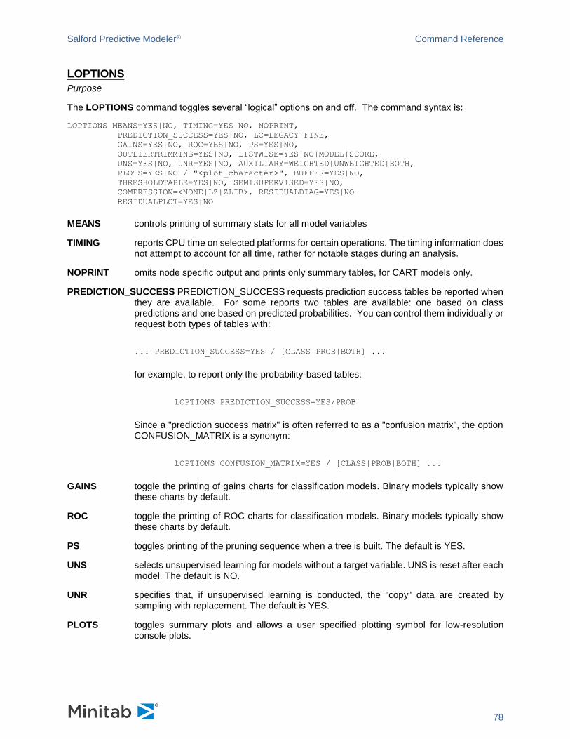
Salford Predictive Modeler® Command Reference
78
LOPTIONS
Purpose
The LOPTIONS command toggles several “logical” options on and off. The command syntax is:
LOPTIONS MEANS=YES|NO, TIMING=YES|NO, NOPRINT, PREDICTION_SUCCESS=YES|NO, LC=LEGACY|FINE, GAINS=YES|NO, ROC=YES|NO, PS=YES|NO, OUTLIERTRIMMING=YES|NO, LISTWISE=YES|NO|MODEL|SCORE, UNS=YES|NO, UNR=YES|NO, AUXILIARY=WEIGHTED|UNWEIGHTED|BOTH, PLOTS=YES|NO / "<plot_character>", BUFFER=YES|NO, THRESHOLDTABLE=YES|NO, SEMISUPERVISED=YES|NO, COMPRESSION=<NONE|LZ|ZLIB>, RESIDUALDIAG=YES|NO RESIDUALPLOT=YES|NO
MEANS controls printing of summary stats for all model variables
TIMING reports CPU time on selected platforms for certain operations. The timing information does not attempt to account for all time, rather for notable stages during an analysis.
NOPRINT omits node specific output and prints only summary tables, for CART models only.
PREDICTION_SUCCESS PREDICTION_SUCCESS requests prediction success tables be reported when they are available. For some reports two tables are available: one based on class predictions and one based on predicted probabilities. You can control them individually or request both types of tables with:
... PREDICTION_SUCCESS=YES / [CLASS|PROB|BOTH] ...
for example, to report only the probability-based tables:
LOPTIONS PREDICTION_SUCCESS=YES/PROB
Since a "prediction success matrix" is often referred to as a "confusion matrix", the option CONFUSION_MATRIX is a synonym:
LOPTIONS CONFUSION_MATRIX=YES / [CLASS|PROB|BOTH] ...
GAINS toggle the printing of gains charts for classification models. Binary models typically show these charts by default.
ROC toggle the printing of ROC charts for classification models. Binary models typically show these charts by default.
PS toggles printing of the pruning sequence when a tree is built. The default is YES.
UNS selects unsupervised learning for models without a target variable. UNS is reset after each model. The default is NO.
UNR specifies that, if unsupervised learning is conducted, the "copy" data are created by sampling with replacement. The default is YES.
PLOTS toggles summary plots and allows a user specified plotting symbol for low-resolution console plots.
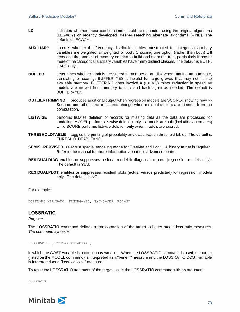
Salford Predictive Modeler® Command Reference
79
LC indicates whether linear combinations should be computed using the original algorithms (LEGACY) or recently developed, deeper-searching alternate algorithms (FINE). The default is LEGACY.
AUXILIARY controls whether the frequency distribution tables constructed for categorical auxiliary variables are weighted, unweighted or both. Choosing one option (rather than both) will decrease the amount of memory needed to build and store the tree, particularly if one or more of the categorical auxiliary variables have many distinct classes. The default is BOTH. CART only.
BUFFER determines whether models are stored in memory or on disk when running an automate, translating or scoring. BUFFER=YES is helpful for large groves that may not fit into available memory. BUFFERING does involve a (usually) minor reduction in speed as models are moved from memory to disk and back again as needed. The default is BUFFER=YES.
OUTLIERTRIMMING produces additional output when regression models are SCOREd showing how R-Squared and other error measures change when residual outliers are trimmed from the computation.
LISTWISE performs listwise deletion of records for missing data as the data are processed for modeling. MODEL performs listwise deletion only as models are built (including automates) while SCORE performs listwise deletion only when models are scored.
THRESHOLDTABLE toggles the printing of probability and classification threshold tables. The default is THRESHOLDTABLE=NO.
SEMISUPERVISED. selects a special modeling mode for TreeNet and Logit. A binary target is required. Refer to the manual for more information about this advanced control.
RESIDUALDIAG enables or suppresses residual model fit diagnostic reports (regression models only). The default is YES.
RESIDUALPLOT enables or suppresses residual plots (actual versus predicted) for regression models only. The default is NO.
For example:
LOPTIONS MEANS=NO, TIMING=YES, GAINS=YES, ROC=NO
LOSSRATIO
Purpose
The LOSSRATIO command defines a transformation of the target to better model loss ratio measures. The command syntax is:
LOSSRATIO [ COST=<variable> ]
in which the COST variable is a continuous variable. When the LOSSRATIO command is used, the target (listed on the MODEL command) is interpreted as a "benefit" measure and the LOSSRATIO COST variable is interpreted as a "loss" or "cost" measure.
To reset the LOSSRATIO treatment of the target, issue the LOSSRATIO command with no argument
LOSSRATIO

Salford Predictive Modeler® Command Reference
80
LTCROSSOVER
Purpose
The LTCROSSOVER command command defines the beginning and end of the learn and test samples. (The LTCROSSOVER command overrides the PARTITION command.) The learn and test samples then
can be "rolled" through the use of the AUTOMATE LTCROSSOVER feature. The command syntax is:
LTCROSSOVER <variable> / VALUE=<x1>, LWIDTH=<x2>, TWIDTH=<x3>
Used by itself, the LTCROSSOVER command offers a way to define learn and test samples. The learn
sample will be composed of all records for which the value of <variable> lies below or at <x>.
Similarly, the test sample will be composed of all records for which the value of <variable> lies above
<x>. Thus, the two samples "abut" each other but there is no overlap. To limit the size of either sample,
use the LWIDTH (for learn) and TWIDTH (for test) options, in which case the records nearest to VALUE will
be included up to the stated width of each sample. Note that LWIDTH and TWIDTH correspond to units of
the crossover variable; they are not record counts. For instance, if your data consisted of quarterly financial reports and you wished to run LTCROSSOVER based on shifting years, and wished to constrain
the test sample to have no more than 10 years of data, you might use the commands: LTCROSSOVER YEAR / VALUE=1984, TWIDTH=10
MADDITIVE
Purpose
MARS only. The MADDITIVE command specifies variables that, if they are part of a MARS model, will enter the model only additively. This applies to both ordinal and categorical variables.
The command syntax is:
MADDITIVE <variable>, ...
To reset, issue the command with no variables:
MADDITIVE
This command is mutually exclusive with MLINEAR. In other words, a variable should be listed on one or the other command, but not both.
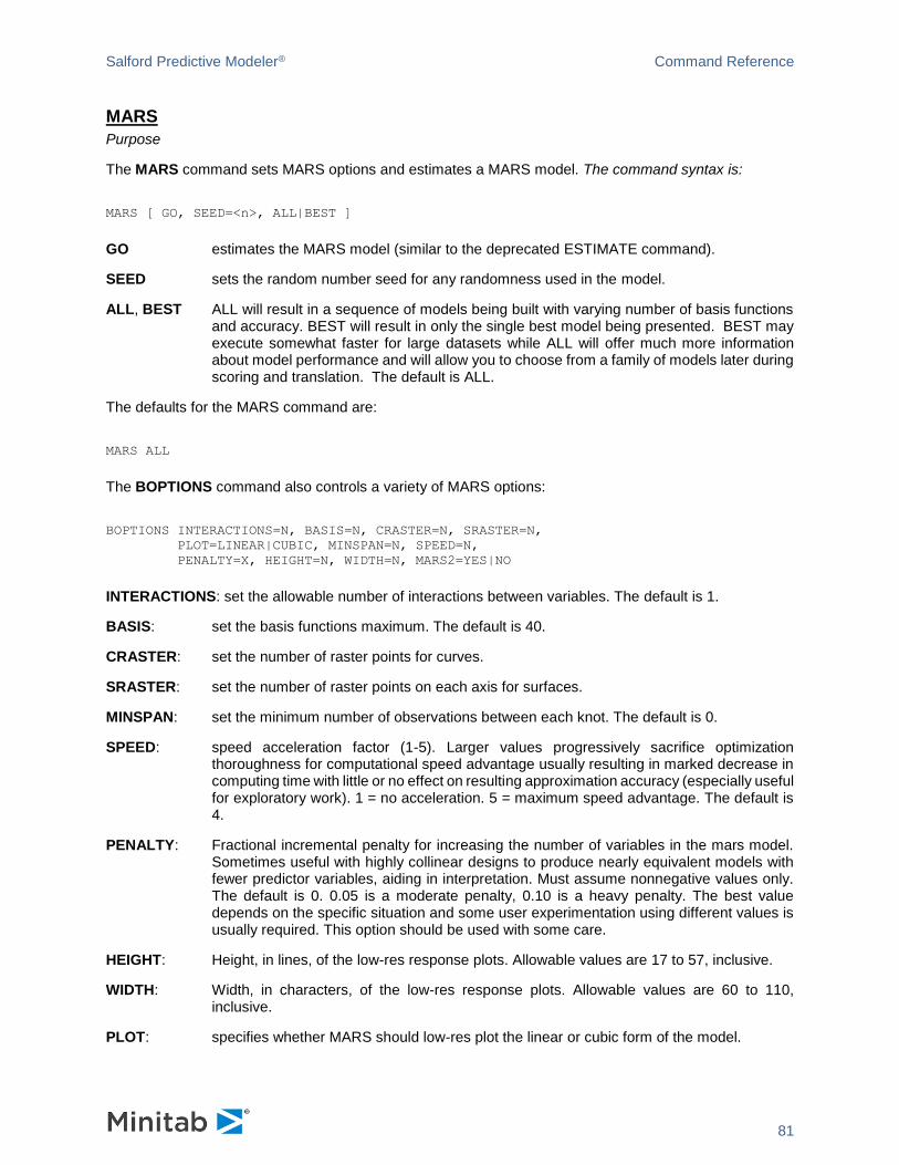
Salford Predictive Modeler® Command Reference
81
MARS
Purpose
The MARS command sets MARS options and estimates a MARS model. The command syntax is:
MARS [ GO, SEED=<n>, ALL|BEST ]
GO estimates the MARS model (similar to the deprecated ESTIMATE command).
SEED sets the random number seed for any randomness used in the model.
ALL, BEST ALL will result in a sequence of models being built with varying number of basis functions and accuracy. BEST will result in only the single best model being presented. BEST may execute somewhat faster for large datasets while ALL will offer much more information about model performance and will allow you to choose from a family of models later during scoring and translation. The default is ALL.
The defaults for the MARS command are:
MARS ALL
The BOPTIONS command also controls a variety of MARS options:
BOPTIONS INTERACTIONS=N, BASIS=N, CRASTER=N, SRASTER=N,
PLOT=LINEAR|CUBIC, MINSPAN=N, SPEED=N,
PENALTY=X, HEIGHT=N, WIDTH=N, MARS2=YES|NO
INTERACTIONS: set the allowable number of interactions between variables. The default is 1.
BASIS: set the basis functions maximum. The default is 40.
CRASTER: set the number of raster points for curves.
SRASTER: set the number of raster points on each axis for surfaces.
MINSPAN: set the minimum number of observations between each knot. The default is 0.
SPEED: speed acceleration factor (1-5). Larger values progressively sacrifice optimization thoroughness for computational speed advantage usually resulting in marked decrease in computing time with little or no effect on resulting approximation accuracy (especially useful for exploratory work). 1 = no acceleration. 5 = maximum speed advantage. The default is 4.
PENALTY: Fractional incremental penalty for increasing the number of variables in the mars model. Sometimes useful with highly collinear designs to produce nearly equivalent models with fewer predictor variables, aiding in interpretation. Must assume nonnegative values only. The default is 0. 0.05 is a moderate penalty, 0.10 is a heavy penalty. The best value depends on the specific situation and some user experimentation using different values is usually required. This option should be used with some care.
HEIGHT: Height, in lines, of the low-res response plots. Allowable values are 17 to 57, inclusive.
WIDTH: Width, in characters, of the low-res response plots. Allowable values are 60 to 110, inclusive.
PLOT: specifies whether MARS should low-res plot the linear or cubic form of the model.

Salford Predictive Modeler® Command Reference
82
MARS2: specifies whether certain computational idiosyncrasies are handled as in MARS v. 2. Setting this option may help produce results that better match those of MARS v2. For normal use, if is recommended that this option be left off (MARS2=NO).
MARS now defaults to limiting the depth of interactions of missing value indicators to the depth specified on your interactions option plus one. To use the previous unlimited convention specify
MARS ... OLDMISSNEST=YES
Saving MARS Basis Functions: You can save all of the basis functions of the largest model built via the SCORE command using the BASIS option. Thus:
BOPTIONS BASIS=30 INTERACTIONS=3
MARS GO
SAVE "myfile.csv"
SCORE BASIS=YES GO
will generate up to 30 basis functions during the forward stepping and then save them all to an output data set. You can view this as a form of intelligent auto-generation of new features.
This allows you to use all of the BFs in the construction of new models including GPS models to arrive at an alternative "optimal" MARS model.
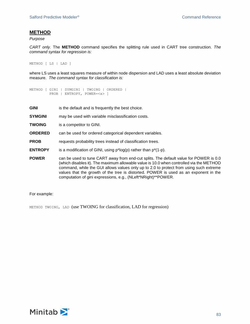
Salford Predictive Modeler® Command Reference
83
METHOD
Purpose
CART only. The METHOD command specifies the splitting rule used in CART tree construction. The command syntax for regression is:
METHOD [ LS | LAD ]
where LS uses a least squares measure of within node dispersion and LAD uses a least absolute deviation measure. The command syntax for classification is:
METHOD [ GINI | SYMGINI | TWOING | ORDERED |
PROB | ENTROPY, POWER=<x> ]
GINI is the default and is frequently the best choice.
SYMGINI may be used with variable misclassification costs.
TWOING is a competitor to GINI.
ORDERED can be used for ordered categorical dependent variables.
PROB requests probability trees instead of classification trees.
ENTROPY is a modification of GINI, using p*log(p) rather than p*(1-p).
POWER can be used to tune CART away from end-cut splits. The default value for POWER is 0.0 (which disables it). The maximum allowable value is 10.0 when controlled via the METHOD command, while the GUI allows values only up to 2.0 to protect from using such extreme values that the growth of the tree is distorted. POWER is used as an exponent in the computation of gini expressions, e.g., (NLeft*NRight)**POWER.
For example:
METHOD TWOING, LAD (use TWOING for classification, LAD for regression)

Salford Predictive Modeler® Command Reference
84
MISCLASS
Purpose
The MISCLASS command specifies misclassification costs. The command syntax is:
To specify other than unit costs, use one of the following command forms:
MISCLASS COST = <x> CLASSIFY <n>|_ALL_ AS <m> [, / COST = .. CLASSIFY .]
MISCLASS COST = <x> CLASSIFY <n> AS <m>|_ALL_ [, / COST = .. CLASSIFY .]
Either a single class or the token _ALL_ may be used before the AS clause. Similarly following the AS clause. For example, the cost of misclassifying class 2 as class 4 is 4.5:
MISCLASS COST=4.5 CLASSIFY 2 AS 4
The cost of misclassifying a woman as a man is 2:
MISCLASS COST=2 CLASSIFY "Female" AS "Male"
The cost of misclassifying a case from classes other than 6 as a class 6 case is 2.75:
MISCLASS COST=2.75 CLASSIFY _ALL_ AS 6
MISCLASS commands are cumulative -- each command will specify a part of the misclassification matrix. To reset the matrix use
MISCLASS UNIT
MLINEAR
Purpose
MARS only. The MLINEAR command specifies variables that, if they are part of a MARS model, will enter the model only linearly. This applies to ordinal variables only. The command syntax is:
MLINEAR <variable>, ...
To reset, issue the command with no variables:
MLINEAR
This command is mutually exclusive with MADDITIVE. In other words, a variable should be listed on one or the other command. Any CATEGORICAL variable included in the MLINEAR command will be ignored.
Salford Predictive Modeler® Command Reference
85
MODEL
Purpose
The MODEL command The command syntax is:
MODEL <depvar> [ = <indep_list> ]
in which <depvar> is the dependent variable (target) and <indep_list> is an optional list of potential predictor
variables. If no <indep_list> is specified, predictor variables are either (1) identified on the KEEP command,
(2) identified by not appearing on the EXCLUDE command, or (3) are all possible variables other than the target and weight if no KEEP or EXCLUDE commands are issued.
Examples:
MODEL DIGIT (all other possible variables used as predictors)
MODEL WAGE = AGE - IQ , EDUC, FACTOR(3-8) , RACE (selected variables) MODEL CLASS = PRED(8) + VARA-VARZ + PRED(1-3)
See the KEEP and EXCLUDE commands for alternative ways to restrict the list of candidate predictor variables. Lists of variables defined via the GROUP (or VARGROUP) command may also be used on the MODEL statements.
MONOTONE
Purpose
CART only. The MONOTONE command allows you to constrain the direction of the impact of a predictor in a TreeNet gradient boosting model. For example, if you want to constrain the impact of a price increase on sales volume to negative (downward sloping demand curve) you can use the MONOTONE command.
Monotonicity will be maintained in the model as you specify while allowing for the monotone variable to interact with other variables. Be aware that if the constraints you impose are inconsistent with the patterns actually in the data model performance can suffer substantially. Its syntax is:
MONOTONE UP [ = <variable1>, <variable2>, ... ]
MONOTONE DOWN [ = <variable1>, <variable2>, ... ]
For example:
MONOTONE UP=PRICE,INCOME,TAX_RATE
MONOTONE DOWN=AGE,WEIGHT,DISCOUNT
To reset all monotone predictor settings, use:
MONOTONE (no predictors will be treated in a monotone manner)
To reset just the increasing or decreasing group of monotone predictors, use:
MONOTONE UP (resets which predictors will be treated monotone increasing)
MONOTONE DOWN (reset which predictors will be treated monotone decreasing)
Salford Predictive Modeler® Command Reference
86
MOPTIONS
Purpose
CART Ensembles only. The MOPTIONS command sets options for a subsequent n ensemble of CART trees). The data are split into a "set-aside" set and an "overall" set. Trees are built and pruned using "overall" data, and are evaluated using "set-aside" data. From the "overall" set are constructed learn and test samples for each of the trees in the expert series. These samples may be copies of the "overall" data, or may be sampled with or without replacement from the "overall" set. It is not necessary to have a test set for each tree -- they can be built using cross-validation or with no pruning (exploratory). It is not necessary to have a set-aside set, although without it comparison of the initial tree and expert set must be done with two additional, separate case runs. The ERROR command settings are ignored during COMBINE set runs. may be sampled with or without replacement from the "overall" set. It is not necessary to have a test set for each tree -- they can be built using cross-validation or with no pruning (exploratory). It is not necessary to have a set-aside set, although without it comparison of the initial tree and expert set must be done with two additional, separate case runs. The ERROR command settings are ignored during COMBINE set runs. The command syntax is:
MOPTIONS TREES=<N>,
SETASIDE=NONE|PROP=<x>|FILE=<file>|SEPVAR=<var>,
TEST|CROSS=<N>|EXPLORE,
DETAILS=INITIAL|SET|ALL|NONE,
LROOT=<file>, ARC=<yes|no>,
TRIES=<N>, POWER=<X>,
RTABLES=<yes|no>, LDRAW=<n>
The TEST, CROSS, and EXPLORE options are used to specify if, and how, pruning is conducted. They are mutually exclusive options.
TREES the number of desired trees in the ensemble, not including any initial tree.
SETASIDE Specifies how the "set-aside" sample is created. This sample is NOT used to build or prune any of the trees. It is only used to evaluate the predictive capability of trees only, including the initial tree.
NONE no set-aside sample will be used.
PROP=<x> a proportion (0 to 1) drawn from the USE data.
FILE=<file> a separate dataset.
SEPVAR=<var> SEPVAR=<var> named variable separates learn and test samples. The setaside value is 1 for numeric and "TEST" or "test" for character variables.
TEST Specifies that the unsampled training data is to be used as a test sample to prune each tree.
CROSS Specifies that N-fold cross-validation is used for each tree in the series, in lieu of a test sample. If <N> is not specified, it defaults to 10.
ARC specifies which combine method will be used. When ARC=YES, the ARCing (Adaptive Resampling and Combining) method is used. When ARC=NO, the bootstrap aggregation (or bagging) method is used. The default is ARC=NO.
EXPLORE Specifies that no test sample or cross validation is to be used for each tree.
TRIES There are occasionally times when CART cannot build one of the trees in the series. You can specify how many times CART should draw and redraw learn and test samples in an effort to get it built. The default is 3.
Salford Predictive Modeler® Command Reference
87
POWER This is the exponent K in the ARC function, evaluated for each observation in the overall set:
arc_func = (1+m(i)^k) / sum_j (1+m(j)^k)
A value of 0 effectively turns ARC off.
RTABLES CART can produce tables that summarize how observations in the overall set are being repeated into the learn and test samples, both for each tree and cumulatively at the end of the series.
DETAILS This controls whether CART produces detailed output (tree sequence, node details, etc) for the initial tree and for each tree in the series.
LDRAW controls the size of the bootstrapped learn sample for non-ARCing models. By default, each bootstrapped sample will be as large as the unsampled learning sample. LDRAW can be used to specify that the bootstrapped sample be smaller or larger. The minimum value permitted is 100, and the bootstrapped sample will be capped at 10 times the size of the unsampled data.
LROOT if the learn sample is sampled for each model, the LROOT option specifies a series of files in which to store the bootstrapped learn samples.
NAMES
Purpose
The NAMES command lists the variables on the current data set. The command syntax is:
NAMES
If you wish to have the list of names appear in your output file, type: NAMES ECHO
NEW
Purpose
The NEW command resets all SPM-specific options while leaving global options (USE file, etc.) in effect. The command syntax is:
NEW
If you wish to also detach from your input dataset, type: NEW DETACH
If you wish to also reset all control parameters to their engine defaults setting, type: NEW CLEAR
Salford Predictive Modeler® Command Reference
88
NOTE
Purpose
The NOTE command lets you write comments on your output. A note can span any number of lines, but no line may be more than 150 characters long. You can embed an apostrophe in a note if you enclose the line in double quotation marks. You can embed double quotation marks if you enclose the line in apostrophes (single quotation marks). A number without quotation marks sends the corresponding ASCII character to the current output device. The command syntax is:
NOTE <#> '<$>','<...>', <#>
Examples:
NOTE 'THIS IS A COMMENT.' 'This is second line of comment.',
"It's the third line here!'"
NOTE 12 'This the top of a new page' (ASCII character 12 and then the string).
OPTIONS
Purpose
The OPTIONS command displays the general options currently in effect including the currently used dataset, any weighting, stratification or selection in effect, number of decimal places to which output prints, and the output destination. The command syntax is:
OPTIONS
OUTPUT
Purpose
The OUTPUT commandfile. If you send output to a file and specify a simple filename, SPM automatically gives the file a ".DAT" extension. If you supply a complete path name for the file you must enclose the name in quotes. If you send output to a file, analysis results also appear on the console/display/classic output. The command syntax is:
OUTPUT * | <file>
Examples:
OUTPUT * (sends subsequent output to screen only)
OUTPUT FILE1 (sends output to FILE1.DAT) OUTPUT 'C:\REPORTS\NEWOUT.LST'
PARTITION
Purpose
The PARTITION command defines how a single input dataset is to be partitioned into learn, test and holdout samples. There are four options: (1) specify the proportions numerically, (2) specify a variable which flags
Salford Predictive Modeler® Command Reference
89
the partition of each record, (3) specify cross validation and an optional cv-binning variable, or (4) request that no partitioning be done (no test data, exploratory modeling):
PARTITION [ LEARN=<x>, TEST=<x>, HOLDOUT=<x>, FAST|EXACT ]
PARTITION SEPVAR=<variable>
PARTITION CROSS [ = <n> | <variable>, OOB=<"filename.ext"> ]
PARTITION FILE="filename.ext"
PARTITION NONE
PARTITION SCORE=<YES|NO>
For instance, to specify that 20% of the data should be allocated for testing purposes and 25% as holdout data:
PARTITION TEST=.2, HOLDOUT=.25
In the above example, the LEARN option does not appear so the amounts specified for test and holdout samples must be expressed as proportions between 0 and 1 and must sum to less than 1. If you specify the LEARN option, then the amounts will be normalized to sum to 1.0, such as in:
PARTITION LEARN=20, TEST=12, HOLDOUT=8
The above would result in 50% of the data into the learn sample, 30% for the test sample and 20% for the holdout sample. SPM offers two modes in which the random separation can be done: FAST and EXACT. FAST provides agreement with past versions of SPM software and is the default, and does independent random draws per record. EXACT carries out a random draw/sort step before the data are processed, producing final partition-specific record counts that are likely to be exactly, or very close, to what one would expect, but with a small time cost.
If the test sample is contained in a separate dataset, use FILE=, for example:
PARTITION FILE="test_sample_0376.xls"
If you use the FILE option you will not be able to allocate a HOLDOUT partition. All the
data in your active file (the file referenced with the USE command) will be used for
LEARN and all the data in the other file will be used for TEST.
For exploratory modeling with no test or holdout samples:
PARTITION NONE
The above would result in all of the data used in the learn sample, while
PARTITION SEPVAR=PURPOSE$
specifies a character variable which should take on values “LEARN” or “Learn”, "TEST" or "Test", "HOLDOUT" or "Holdout".
For a numeric separation variable, such as
PARTITION SEPVAR=USAGE
a value of 0 indicates the record is part of the LEARN partition, and 1 and -1 indicate TEST and HOLDOUT respectively.

Salford Predictive Modeler® Command Reference
90
Cross validation is requested with a command like:
PARTITION CROSS=10
If you have a variable that contains the cross validation bins you can use this to control the cross validation process with:
PARTITION CROSS=CVBINVAR
PARTITION CV is a synonym for PARTITION CROSS. During cross-validation, the OOB option saves a prediction for each record produced by the appropriate sized model when that record is in the test partition. (OOB stands for "out of bag"). The OOB option will have no effect if the testing method is other than cross validation.
During each cross-validation fold SPM produces model predictions for all records in the fold's test partition. When all folds of cross-validation have completed we will have an OOB prediction for every record in the LEARN.
For engines listed below each record will receive one OOB prediction as follows:
CART: OOB prediction for each pruning in the tree sequence. There may be dozens, hundreds, and in some cases thousands of such prunings so you may want to limit the CART tree growth before requesting this data.
MARS: OOB prediction for each number of basis functions in model sequence
TN: OOB prediction for the optimal model for each performance criterion (likelihood, accuracy, ROC, lift) and also the 1-tree and max-tree models. For binary classification models we typically produce 6 OOB estimates for each record, corresponding to 6 different sized models.
GPS: OOB prediction for the optimal elasticity at each point evaluated on the path.
To save merge keys, ID variables, or predictors to the OOB file use the IDVAR command to explicitly list the variables to be saved, as in:
IDVAR X1, X2, X3
PARTITION SCORE=YES will result in the model being scored immediately after it is built, keeping scoring statistics for learn, test and holdout samples separate. Without this option, immediate scoring after a model is built will only occur if there is a holdout sample.
Note that the DATASHIFT command offers another way of separating your data into learn and test samples. When the DATASHIFT command is used with the AUTOMATE DATASHIFT feature, the result is a powerful tool for building a series of models on a systematically varied series of learn and test samples.
+++++++++++++++++++++++++++++++++++++++
NOTE: Additional technical notes are as follows.
The PARTITION controls the division of your data into these training and testing/evaluation roles:
LEARN (also referred to as TRAIN)
TEST
HOLDOUT (this partition is optional and must be explicitly requested;
it is never generated automatically)
Salford Predictive Modeler® Command Reference
91
PARTITION also allows for CROSS-VALIDATION, data partitions to exist in different physical files, the possibility that the data will not be partitioned at all.
The most common use of PARTITION for smaller data sets would be something like:
PARTITION CROSS=10 or
PARTITION CV=10
which calls for 10-fold cross-validation. You can request other numbers, of folds, for example, 2 or 5 or 20, or even as many folds as there are records in your data.
Another common pattern would be something like
PARTITION TEST=.2
This would randomly divide the data into an 80% train and a 20% test partition. We only create a HOLDOUT partition if this is explicitly requested. Thus,
PARTITION TEST=.2, HOLDOUT=.2
would allocate 60% to train, 20% to test and 20% to holdout. Observe that the command above did not mention LEARN. It is good form to explicitly list all the partitions you wish to use, as in
PARTITION LEARN=.8 TEST=.2
(Note that some authors use the term "validate" to refer to this test partition, and they use "test" to refer to what we call "holdout". But the usage can be inconsistent and we thus prefer our terminology which makes the roles of the partitions easier to remember.).
It can be very helpful to assign data records to partitions prior to analysis via the use of a SEPVAR. This is a "separation variable" containing 2 or 3 values corresponding to the partitions you plan to use.
For a NUMERIC sepvar, (lets call it SAMPLE) we recognize these values
SAMPLE PARTITION
=======================================
0 LEARN partition
1 TEST partition
-1 HOLDOUT partition (optional)
If your SAMPLE variable contains just 0s and 1s then we will have just LEARN and TEST partitions.
If you prefer a CHARACTER sepvar, such as PARTITION$, its values should be:
"LEARN"
"TEST"
"HOLDOUT"
A final detail: the PARTITION command recognizes the keywords FAST and EXACT which are relevant to random partitioning. The FAST option assigns records to partitions "on-line" meaning that for every record encountered we use a random number draw to determine that record's assigned partition. Since each record is assigned in isolation there is no guarantee that you will end up with the partition proportions you requested. For example, suppose you request
Salford Predictive Modeler® Command Reference
92
PARTITION LEARN=.5 TEST=.5 FAST
you can expect the two data partitions to be approximately equal. But chance draws may result in non-trivial deviations from the 50/50 division. This is just like tossing a fair coin many times; we expect the fraction of HEADS and TAILS to be similar but in any specific sequence of tosses there can be substantial deviations, especially in smaller samples.
PARTITION LEARN=.5 TEST=.5 EXACT
is designed to give you EXACTLY equal partitions (plus or minus one record). To do this we must operate on all of the data at once. Keep in mind that later operations that you request such as deletion of records or operation on a specified subset of the data via the SELECT command can cause the realized partition fractions to deviate from exact fractions.
PENALTY
Purpose
The PENALTY command defines a variety of penalties on predictors in CART, TreeNet, MARS, and GPS models. The command syntax is:
PENALTY <var1>=<pen1> [ , <var2>=<pen2>, ...
/ MISSING=<xm1>,<xm2>,
HLC=<xh1>,<xh2>,
BIAS=<xb1>,<xb2>,<xba>,
CONTBIAS=<xb1>,<xb2>,<xba>,
CATBIAS=<xb1>,<xb2>,<xba>,
BIASMODE=<0,1,2>,
CARDINALITY=<xc1>,<xc2>,
SURROGATE=<YES|NO> ]
CART, TreeNet, and Random Forest Models
Penalties for CART, TreeNet and RandomForests models operate similarly, inhibiting splits from being formed, with the exception of CART surrogates explained below.
By default, no variable-specific penalty is applied to a variable's improvement when considering the variable in a model (although a penalty for missing data may be in effect). The PENALTY command
specifies a multiplicative fraction between 0 and 1 used to downweight the improvement, thus making it more difficult for the predictor in question to be chosen in relation to other predictors. Specifically, the improvement evaluated for <var1> is multiplied by 1-<pen1>. Values specified by <pen> should be between 0 and 1, and are reset to 0.0 if specified outside that range [0,1].
Four additional types of improvement penalties may be specified. The MISSING, HLC, BIAS and CARDINALITY options may be given after the slash.
MISSING To penalize variables that have a large proportion of missing values in the partition (node) being split, the MISSING option is used. This option allows significance of the primary splitters and all competitors to be weighted by a simple function of the percentage of cases present (nonmissing) in the node partition. The expression or weighting the significance is:
improvement = improvement * factor
in which factor=1.0 if there are no missing values and
Salford Predictive Modeler® Command Reference
93
factor = xm1 * ( fract ^ xm2 )
if there are missing values. Fract is the proportion of observations in the partition (node) that have nonmissing values for the splitter in question. If xm1 and xm2 are set to values that result in taking a root of a negative number, or result in improvement < 0, improvement is set to 0. If improvement > 1, it is set to 1.
HLC To penalize categorical splitters that have a high number of levels relative to the number of records in the partition (node), the HLC option is used. Consider the expression:
ratio = log_base_2 ( N records in node ) / ( N categories - 1 )
The HLC option weights the improvement of primary splitters and all competitors by the following function:
improvement = improvement * factor
in which factor=1.0 if ratio => 1.0 and
factor = 1 - xh1 + xh1 * ( ratio ^ xh2 )
if ratio < 1.0. If xh1 and xh2 are set to values that result in taking a root of a negative number, or result in improvement < 0, improvement is set to 0. If improvement > 1, it is set to 1.
CARDINALITY is just like HLC, except that CARDINALITY operates on continuous predictors and focuses on the number of distinct values a continuous predictor takes on in a node.:
Surrogate Penalty
For CART, which supports surrogate splits, the improvement penalties are applied to surrogates in the same way that they are applied to competitors. To disable penalties for surrogates in CART, use the SURROGATE=NO option:
PENALTY ... / ... SURROGATE=NO ...
TreeNet and RandomForests do not support surrogate splits, so the
SURROGATE option has no effect on those models.
Bias Penalty in CART, RF
The short form of this command is:
PENALTY ... / BIAS=<HLC1>,<HLC2>,<ALPHA>
where the three user set tuning parameters HLC1, HLC2, and ALPHA are briefly described next. The longer form of the command allows different values of these parameters to be set for continuous and categorical predictors:
PENALTY / CONTBIAS=<HLC1>,<HLC2>,<ALPHA>, CATBIAS=<HLC1>,<HLC2>,<ALPHA>
The essence of the possible "bias" in tree-based splitter selection is that predictors with a greater number of distinct values have an "advantage" in splitting. We discuss this topic at length in technical papers and here just describe how our penalties function.
Salford Predictive Modeler® Command Reference
94
A key ratio describing a potential predictor in the training data is the ratio of number of observations to the number of distinct predictor values. This ratio is expressed as
RATIO = log_2(NOBS)/log_2(NVALUES) for continuous predictors and
RATIO = log_2(NOBS) / (J-1) where J is the number of levels for categorical
predictors
We determine how much we want to damp this ratio with the user set tuning parameter ALPHA
DRATIO = 1 + ALPHA*LN(RATIO) + (1-ALPHA)*ln(1 + ln(RATIO))
with the default ALPHA=0. Observe that RATIO is defined in terms of log base 2 while DRATIO uses a
natural log.
DRATIO allows us to move between a log (moderate) and a log-log (heavy) damping of the ratio with our
recommendation to start with log-log.
With DRATIO computed we create a "penalty" that follows the pattern of our HLC penalty. First, the
DRATIO may be raised to a power which we typically set to 1.0 although values ranging from .25 to 5.0
could be useful. We refer to this as the "power" parameter (HLC2).
The final improvement adjustment expression is
"penalty" = 1 - HLC1 + HLC1*RATIO^HLC2
where HLC1 is a user set tuning parameter between 0 and 1. The "penalty" multiplies the improvement
score of any potential splitter. When its value is greater than 1.0 the "penalty" is actually a booster that favors a predictor.
Our "penalty" can be seen as a weighted average of 1 and DRATIO^HLC2 with weights (1-HLC1) and
HLC1. If HLC1 is set to 1.0 then we work only with the power modified DRATIO and clearly if HLC1=0 we
cancel any penalty. Values between 0 and 1 move the adjustment term towards 1 and thus diminish the adjustment.
The "penalty" can and probably should be tuned separately for continuous and categorical variables
With three free parameters for each of continuous and categorical predictors, the tuning of these adjustments can be complicated and we therefore recommend that modelers start with the AUTOMATE
BIASPENALTY to conduct a randomized search over plausible settings.
GPS Models:
The PENALTY syntax described above for CART and TreeNet models applies to GPS models also except that only variable-specific penalties are used in GPS (the MISSING, HLC, BIAS and SURROGATE options are ignored for GPS models). The variable-specific penalties must simply be positive (they are not clipped to the range [0,1] as they are for CART and TreeNet). In GPS, these variable-specific penalties are used as a divisor to the gradient component which is used to select the next active predictor (determining which coefficient will be updated). GPS models produce multiple effects for categorical predictors (i.e., 0/1 dummies), in which case the same penalty is applied to all effects for a given predictor.
MARS Models:
The PENALTY syntax described above for CART and TreeNet models applies to MARS models too, including the MISSING and HLC options (SURROGATE is ignored since MARS has no concept of surrogates). The variable- specific penalties must be in the range [0,1] as they are for CART and
Salford Predictive Modeler® Command Reference
95
TreeNet. MARS has the concept of "favor variable(s) into the model", a measure which is multiplied by 1 - <pen>. In this way, variable- specific penalties in MARS are similar to those in CART and TreeNet: multiplicitive downweighting inhibits a predictor from being selected into the model. Variable groups may be used in the PENALTY command similarly to variable names.
Variable groups may be used in the PENALTY command similarly to variable names.
PIPELINE
Purpose
The PIPELINE command specifies a pair of models, the first of which feeds into the second. Its syntax is:
PIPELINE STAGE1=<engine>, STAGE2=<engine>, REPORT=<report_type>
in which engine is one of compute engines: CART, TREENET, MARS, LOGIT, PROBIT. <report_type> specifies certain reporting options that provided enhanced detail above and beyond the default. At present only certain engine combinations are supported.
PLOT
Purpose
The PLOT command produces 2-D scatter plots, plotting one or more y variables against an x variable in separate graphs. The command syntax is:
PLOT <yvar1> [, <yvar2> , <yvar3> ] * <xvar> [ / FULL, TICKS | GRID, WEIGHTED, BIG ]
The console plot (low-resolution, non-GUI) is normally a half screen high: the FULL and BIG options will increase it to a full screen (24 lines) or a full page (60 lines).
TICKS and GRID add two kinds of horizontal and vertical gridding.
WEIGHTED requests plots weighted by the WEIGHT command variable.
Examples:
PLOT IQ*AGE / FULL, GRID
PLOT LEVEL(4-7)*INCOME / NORMALIZED
PLOT AGE,WAGE,INDIC*DEPVAR(2) / WEIGHTED
Only numerical variables may be specified.
Variable groups may be used in the PLOT command similarly to variable names.
Salford Predictive Modeler® Command Reference
96
PRIORS
Purpose
CART only. The PRIORS command specifies prior class probabilities for classification models. The command syntax is:
PRIORS [ DATA | LEARN | TEST | EQUAL | MIX |
SPECIFY <class1>=<x1>, <class2>=<x2>, ... ]
in which <x1>, <x2>, ... is a vector of real numbers. The options set prior class probabilities as follows:
DATA priors match observed sample shares in combined learn and test data.
LEARN priors match observed sample shares in learn data alone.
TEST priors match observed sample shares in test data alone.
EQUAL uniform priors, automatically set to 1 / (number of classes).
MIX priors set to the average of DATA and EQUAL options.
SPECIFY <class1>=<x1>, <class2>=<x2>,... priors are set to any strictly positive numbers. CART will normalize the values to sum to 1.0. A value must be assigned to each class. For character classes, the class value must be in quotes. The SPECIFY option requires that the dependent variable already be identified on the MODEL command.
Examples:
PRIORS SPECIFY "Coffee"=1, "Tea"=2,
"H2O"=4, "Soda"=1 (explicit list, let CART rescale)
PRIORS EQUAL (the default)
PRIORS MIX (split the difference between DATA and EQUAL)
Purpose
The PRINT command switches you between standard and extended analysis results for statistical procedures. The command syntax is:
PRINT=LONG|MEDIUM|SHORT
You may select LONG for extended results (available from certain procedures), SHORT for standard results, or MEDIUM for somewhat extended results in MGLH and extended results elsewhere. The default is PRINT=SHORT.
Examples:
PRINT=SHORT (produces only standard output from commands)
PRINT=MEDIUM (prints extended output for some procedures and also
prints means and standard deviations for ANOVA)
PRINT=LONG (prints extended output for some procedures)

Salford Predictive Modeler® Command Reference
97
PROBIT
Purpose
The PROBIT command is used to toggle probit model options, and to launch a binary probit model. The command syntax is:
YES | NO options are:
PROBIT MEANS=YES|NO, LOG=YES|NO, COVARIANCE = YES|NO
Numeric options are:
PROBIT CHANGE=<x>, ITERATIONS=<n>
To launch a probit model, use the GO option:
PROBIT ... GO
The MEANS option controls the printing of covariate means after the first pass through the data. LOG shows the parameter, change and gradient vectors, and the Hessian and covariance matrices after each iteration. COVARIANCE prints out the covariance matrix at convergence.
The default values are:
PROBIT CHANGE=.001, ITERATIONS=15
Successive PROBIT statements may be used -- they are cumulative up until the GO option is issued, at which point the model is built. For example:
PROBIT LOG MEANS=NO
PROBIT GO
QUIT
Purpose
The QUIT command terminates the SPM session.
The command syntax is:
QUIT
REFERENCE
Purpose
The REFERENCE command specifies which class is treated as the reference or base (left out) class for a categorical variable. This influences some statistical measures as well as the sign of regression coefficients since the choice of the reference class has a bearing on how the model is expressed or parameterized for Logit and GPS. The command syntax is:
REFERENCE <variable1>=<class1> [, <variable2>=<class2>, ... ]
Salford Predictive Modeler® Command Reference
98
For example:
REFERENCE RESPONSED$="NO"
REFERENCE REGION="Florida", OUTCOME=0, GENDER=1
Unless otherwise specified on the REFERENCE command, the focus class for a categorical variable is:
a) the compliment of the FOCUS class for binary variables,
b) the class that alphanumerically sorts last for multinomial variables.
If the FOCUS and REFERENCE commands are in conflict for a particular variable, for instance because they specify the same class to be both focal class and reference class, the FOCUS command takes precedence. The command syntax is:
REGRESS
Purpose
The REGRESS command performs an OLS regression on the target. The command syntax is:
REGRESS GO [, INTERCEPT=[YES|NO], PERFORMANCE=[YES|NO] ]
INTERCEPT=NO omits the intercept (constant) term from the model.
PERFORMANCE=NO skips computing and reporting detailed performance measures.
The default is:
REGRESS GO, INTERCEPT=YES, PERFORMANCE=YES.
For example:
USE "history.xls"
MODEL AMOUNT
CATEGORY REGION$, EDUCATION_LEVEL
KEEP INCOME<0-5>, REGION$, LIMIT, EDUCATION_LEVEL
REGRESS GO
NOTE: For RIDGE regression see the RIDGE command.
REM
Purpose
The REM command is for comments. All subsequent text on that line is ignored. The REM command is especially useful when writing programs in BASIC and in the writing of command files. The command syntax is:
REM <text>
REM This is a comment line and is not executed

Salford Predictive Modeler® Command Reference
99
RF
Purpose
The RF command builds a RandomForests The command syntax is:
RF [ GO, TREES=<n>, PREDS=<n|SQR|SQR2|SQR5,ALL,BAGGER>,
POST=<YES|NO>, PROXIMAL=<n|AUTO>, PROXACCUM=<ALL|OOB1|OOB2>,
FULLPROX=<YES|NO>, MAXFULL=<n>, RANDOMMODE=<0|1|2>,
OUTLIERS=<YES|NO>, PARCOOR=<n>, PPARCOOR=<YES|NO>,
PCOORSCALE=<YES|NO>, PCOORMIS=<x>, RANDOMSPLITS=<YES|NO>,
NPROTO=<n>, MDSITER=<n>, PROTOREPORT=<YES|NO>, BCORR=<YES|NO>,
NPROXPROTO=<n>, NPROXMDS=<n>, NPROXOUTLY=<n>, CORR=<YES|NO>,
SAVE="filename", SVOOB=<YES|NO>, SVSCALE=<YES|NO>,
SVPARCOOR=<YES|NO>, SVPROX=<YES|NO>, SVMARGIN=<YES|NO>,
SVCLUSTER=<YES|NO>, SVIMPUTED=<YES|NO>, SVPROTOTYPES=<YES|NO>,
LOOK=<n>, BOOT=<n>, SEED=<n>, ADJUSTBOOTSTRAP=<YES|NO>
JOIN=<YES|NO>, CLUSTERS=<n1,n2,...>, BOOTSTRAP=<N|AUTO>,
JITTERSPLITS=<YES|NO>, LEGACYSPLIT=<YES|NO>,
LINKAGE=<ALL|SINGLE|COMPLETE|CENTROID|AVERAGE|MEDIAN|WARD>,
LINKITER=<n>, PMETHOD=<0|1>, MCLASSES=<N>,
MISSING=<FAST|ADVANCED> ]
To reset all RF options, simply issue the RF command alone:
RF
Other commands related to RF are: CW, CATEGORY, ERROR, KEEP, and MODEL.
The RF command options are:
GO launch the model. If this is not specified, the RF command is simply setting options for the next RandomForests model.
TREES=<n> specifies the number of trees that should be built in the Random Forest. The default is 500. The minimum allowable value is 3.
PREDS=<x> specifies the number of randomly-selected predictors used in each tree. The default is 3. You can specify that RF use either the square root of the number of available predictors, twice the square root or half the square root with the following three varieties of the PREDS option:
PREDS=SQR
PREDS=SQR2
PREDS=SQR5
To force RF to consider all predictors at every node, use PREDS=BAGGER. To have RF sample from all predictors at every node, use PREDS=ALL.
LOOK=<n> specifies the interval (number of trees) at which the model progress report should be issued. The default is 10.
SCALE=<n> specifies the number of scaling coordinates that should be extracted, plotted and saved. The default is 5. Setting this to 0 or 1 bypasses the extracting of scaling data.
PROXIMAL=<n|AUTO> specifies the number of records that are tracked for measures. The default is AUTO.
Salford Predictive Modeler® Command Reference
100
PROXACCUM=<ALL|OOB1|OOB2> controls how pairs of records may contribute to the proximity matrices. ALL specifies that any two records that reach the same terminal node of a given tree may contribute. OOB1 requires that at least one of the two records reaching a common terminal node in a given tree be out-of-bag (internal test sample) for the tree. OOB2 requires both records to be out-of-bag. The default is ALL, which results in the most non-zero cells in the proximity matrices (both full and partial).
BOOTSTRAP=<n> specifies the bootstrap sample size. The default is BOOTSTRAP=0 in which case the program estimates an optimal bootstrap sample size.
ADJUSTBOOTSTRAP=<YES|NO> YES will adjust the bootstrap size if it is deemed to be too small relative to the number of trees. However, if you wish to deliberately use very small bootstrap sizes, use NO to avoid adjustment. The default is NO.
SAVE="filename" if specified, defines a root dataset set used when constructing datasets that contain outlier, scale and parallel coordinate measures following the RF run. This must be a fully qualified dataset filename in quotes.
SCW=<x> specifies that target class weights should be normalized to sum to X. Class weights are somewhat akin to inverted priors in CART and by default are not normalized. Setting X to 0.0 or missing (.) turns normalization off, which is the default.
MISSING=<FAST|ADVANCED> selects among two methods by which the RF procedure imputes missing values. FAST uses medians for continuous predictors and modes for discrete predictors. ADVANCED builds ancillary models to determine the best imputation values.
MITERATIONS=<n> specifies how many modeling iterations should be done when ADVANCED missing value imputation is used. The default is 6.
PARCOOR=<n> controls how many parallel coordinate vectors are computed for each target class. PARCOOR=0 disables the computation of parallel coordinates.
PPARCOOR=<YES|NO> controls whether parallel coordinate vectors are printed to the classic output. By default they are not.
PCOORSCALE=<YES|NO> controls whether parallel coordinates data for predictors are scaled or not. The default is YES, in which the scaled values can be interpreted as learn sample percentiles after missing values are imputed with medians. If you select NO, then the parallel coordinates report in the classic output and saved dataset (SVPARCOOR option) will show actual data values. The GUI presentation shows percentiles (scaled predictors) regardless of the PCOORSCALE option. Categorical predictors, which are treated as unordered, are not scaled.
PCOORMIS=<x> Predictors having a greater target-class-specific proportion of missing data than <x> will not be depicted in the parallel coordinates report, dataset, or GUI charts for that target class. The default is PCOORMIS=0.20.
NPROTO=<n> controls how many prototypes are computed for each target class. NPROTO=0 disables the computation of prototypes. The default is 25.
PROTOREPORT=<YES|NO> whether prototypes, if computed, are reported in the classic (text) output stream. The default is NO, because these reports can often be very lengthy.
LINKITER=<n> sets the number of linkage iterations during clustering.
MDSITER=<n> sets the maximum number of iterations allowed when solving for MDS scale dimensions. The default is 1000.
OUTLIERS=<YES|NO> controls whether outlier statistics are computed. The default is YES.
Salford Predictive Modeler® Command Reference
101
SEED=<n> sets the RF random number seed to a value of your choosing. The default is 17395. N must be positive nonzero. Note that random partitioning of learn and test samples during data preprocessing depends on the SEED **command**.
FULLPROX=<YES|NO> The FULLPROX and FPN options are used together to control whether
MAXFULL=<n> a full proximity matrix is attempted. The learn sample must be less than or equal to MAXFULL and FULLPROX must be YES before a full proximity matrix will be attempted. Note that the attempt to allocate the full proximity matrix, which can be very large (order N-squared), may fail in which case the model will proceed without clustering or full proximity data. The default is FULLPROX=YES, MAXFULL=10000.
NPROXPROTO, NPROXMDS, NPROXOUTLY The NPROXPROTO, NPROXMDS and NPROXOUTLY options each set an upper limit on the maximum number of proximal records used in the computation of prototypes, scale and outlier statistics. The default for all these options is 0, which indicates that all available proximal records be used. To increase the number of available proximal records, use the PROX= option.
SVx=<YES|NO> These seven options work with the SAVE option to control saving of selected post-processed data and results. The legacy synonym for each option is shown in parentheses:
SVOOB: predicted probabilities and margins. (SV1).
SVSCALE: MDS scaling coordinates. (SV2).
SVPARCOOR: parallel coordinates plot data (SV3). See the PCS and PARCOOR options for more control.
SVPARTPROX: partial proximity matrix (SV4). Classification only.
SVFULLPROX: full proximity matrix. See FULLPROX and MAXFULL options for more control. Classification and regression models.
SVCLUSTER: cluster assignments produced by JOIN (SV5). Classification only.
SVIMPUTED: saves data after missing value imputation has been done, for classification models only. Requires MISSING=ADVANCED option. Note: a proximity matrix is required for advanced missing value imputation.
SVPROTOTYPES: saves prototypes if available. Classification only.
NOTE: By default, if the SAVE command is used all SVx options are enabled (e.g., SVOOB=YES, SVSCALE=YES, SVPARCOOR=YES, SVPARTPROX=YES, SVCLUSTER=YES, SVIMPUTED=YES, SVPROTOTYPES=YES, SVFULLPROX=YES, SVMARGIN=YES).
JOIN=<YES|NO> requests a joining/clustering using the RF proximity matrix. See CLUSTERS option for controlling the number of clusters.
CLUSTERS=<n, n, …> when JOIN=YES, allows the number of clusters to be specified, otherwise the default is 4, 6, and 10. Useful when the SAVE option is used to save clusters to a dataset.
LINKAGE determines which linkage methods are used in performing the clustering.
POST=<YES|NO> suppresses all post-processing of a categorical RF model, including proximity matrix, prototypes, parallel coordinates, scaling, missing value imputations.
Salford Predictive Modeler® Command Reference
102
Note: to save statistics when building a Random Forests model (RF GO), use the SAVE **option** on the RF command, which will generate a group of datasets with similar filenames. To save statistics when scoring a Random Forests model (SCORE GO), use the SAVE **command** to specify the single output dataset.
PMETHOD Random Forests uses a novel technology to determine variable importance using random data permutations. However, on datasets with many records this feature may result in exceedingly long run times. The following options are available to control the variable importance algorithm:
PMETHOD=0: disables the algorithm altogether and usually results in a significant speed up; note that the traditional Gini-based variable importance is still available.
PMETHOD=1: turns on permutation-based variable importance calculation; may cause a significant slowdown on datasets with many observations but usually runs quickly on wide datasets.
MCLASSES sets the maximum number of classes permitted for predictors. Variables with more than MCLASSES levels will not be used as predictors. The default is 50.
RANDOMSPLITS toggles whether the split points in Random Forests are selected at random (YES) or via improvement maximization (NO).
RANDOMMODE=0|1|2 only affects continuous predictors and only when RANDOMSPLITS=YES. The default is 0. The options are:
0: use predictor distribution when selecting random split point.
1: all possible split points are equally probable, i.e., no accounting for duplicate data points.
2: find min & max of predictor in the node, make a random uniform draw [0,1], split point is then selected within [min,max] based on uniform draw, may result in a split that violates minchild.
LEGACYSPLIT invokes older splitting code. YES may help obtain exact agreement with RF trees built with 8.0.0.671 and earlier versions of SPM. The default is NO.
BCORR implements a suggestion Leo Breiman made in his theoretical paper explaining why Random Forests should be expected to perform well. In the paper, he pointed out that the forest relies on diversity of trees: the more different the individual trees are, the greater the potential benefits from the averaging of their predictions. Classification models only, requires a test sample.
JITTERSPLITS once a split of a node has been determined using only rank order information in the data, an actual split value is computed for the splitter variable by taking the midpoint of the two records on either side of the split. JITTERSPLITS instead selects a random value between these two records instead of the midpoint. JITTERSPLITS might deliver superior results on OOB and TEST data. JITTERSPLITS affects continuous splitters only.
Example 1: build an RF model and save statistics to output datasets:
USE "mydata.xls"
MODEL TARGET
CATEGORY TARGET
RF GO, TREES=300, SAVE="outstats.xls", SV1=YES, SV2=NO, SV3=YES
Salford Predictive Modeler® Command Reference
103
Example 2: build an RF model and score another dataset:
USE "mydata.xls"
MODEL TARGET
CATEGORY TARGET
GROVE "randomforest13.grv"
RF GO
USE "scoringdata.xls"
GROVE "randomforest13.grv"
SAVE "scores_from_forest.xls"
SCORE GO
Random Forests typically creates an automatically sized "out of bag" sample, using learn records that are not selected by bootstrap sampling, to evaluate each tree. However, you can request that the "out of bag" sample be controlled differently:
a) by a user-defined proportion or number of records, which is b) applied to the learn data as a whole or to each target class, and is c) either fixed for all trees or redrawn for each tree. The syntax for controlling these characteristics are:
RF SAMPLEAMOUNT=<AUTO|X|N>, SAMPLEMODE=<FIXED|VARYING>, SAMPLEBYCLASS=<YES|NO>
SAMPLEAMOUNT=AUTO restores the usual behavior of Random Forests, which is to use bootstrap sampling (with replacement) to form the learn sample for each tree, with unselected records becoming the out of bag sample. SAMPLEAMOUNT=<X> specifies a proportion of data to be used as out of bag, with X greater than 0.0 and less than 1.0. SAMPLEAMOUNT=<N> specifies a number of records to be used as out of bag, with N >= 1. If the SAMPLEAMOUNT option is used to control the BOOTSTRAP sampling detail then the ADJUSTBOOTSTRAP option will be ignored.
SAMPLEMODE=VARYING leads to the training and out of bag samples being redrawn for each tree. SAMPLEMODE=FIXED fixes these, drawing them once for the first tree and maintaining them for subsequent trees.
SAMPLEBYCLASS=YES enforces the SAMPLEAMOUNT option for each target class, while SAMPLEBYCLASS=NO only enforces it for the learning data as a whole.
RIDGE
Purpose
The RIDGE command controls ridge regression. The command syntax is:
RIDGE [ GO, BOOTSTRAP=<n>, BALPHA=<x>, LAMBDA=<x>,
START=<x>, END=<x>, INTERVALS=<n> ]
BOOTSTRAP requests bootstrap re-sampling of the learn sample to produce confidence intervals for the coefficient estimates.
BALPHA specifies the alpha for confidence intervals. The default is 0.05.
LAMBDA species the ridge lambda value.
START, END, INTERVAL are used to specify a range of LAMBDA values. A model will be estimated for each lambda value. If there are test data, model performance on the test data will be assessed for each model and the optimal model will be identified.
Salford Predictive Modeler® Command Reference
104
RULELEARNER
Purpose
The RULELEARNER uses a combination of TreeNet trees and GPS generalized lasso models to extra interesting and predictive “rules” from data. The GUI model setup for the RuleLearner engine guides the process. From the command line you must issue these commands in sequence:
GPS RULELEARNER=YES
TREENET GPS=YES GO
NOTE: Additional details are provided in the help entries for GPS and TreeNet.
RUN
Purpose
The RUN command processes the input dataset(s) and produces summary reports, and optionally creates an output dataset. No modeling is done. Variables included in the analysis are (if defined): the target, the KEEP list, any ID variables (the IDVAR command), a CASEID (case identifier pointing to the record number in the original dataset), and a sample indicator if partitioning is in effect. The command syntax is:
RUN [ SAVEPROCESSED=<YES|NO>, SAMPLE="variable_name" ]
If you wish to create a new output dataset, precede RUN with SAVE:
SAVE <filename>
RUN [ SAVEPROCESSED=<YES|NO>, SAMPLE="variable_name" ]
If an output dataset is being created, categorical data will by default be saved to the output dataset in its "natural form". However, if you wish to have categorical data recoded to a contiguous set of integer values (e.g., 1,2,3,...) in the output dataset, use the SAVEPROCESSED=YES option. This can be useful when categorical variables with many distinct classes are used as predictors in some modeling algorithms since they can be treated as continuous variables in this form. The SAMPLE option allows you to specify a particular name for the sample indicator in the saved dataset. For example,
PARTITION TEST=.3,HOLDOUT=.2
SAVE "partitioned.csv"
RUN SAMPLE="INDICATOR$"
would add the character variable INDICATOR$ to the dataset, taking on values "LEARN", "TEST" and "HOLDOUT" to indicate the data samples. Alternatively, if you specified a numeric variable:
RUN SAMPLE="LTH"
the numeric variable LTH would take on values 0 for learn, 1 for test and -1 for holdout. If you do not specify any sample variable name and your data are partitioned, the default name will be SAMPLE$.
Salford Predictive Modeler® Command Reference
105
SAMPLE
Purpose
The SAMPLE command defines target class sampling rates for the learn, test and holdout samples used to build models. It is only appropriate for categorical models. It has no effect on regression models or STATS results. The command syntax is:
SAMPLE LEARN|TEST|VALID <target_class>=<rate>, ...
Some examples are:
SAMPLE LEARN "Nonbuyer"=0.01, "Unknown"=0.25
SAMPLE TEST 0=.5, 1=.5, 2=.90
Rates are expressed as proportions ranging from 0 to 1. Sampling rates of 1.0 are assumed for all target classes, in all samples (learn, test, holdout) unless explicitly defined with the SAMPLE command.
SANITIZE
Purpose
The SANITIZE command creates a copy of your dataset with original variable names replaced by generic names, and without any variable labels. For example:
USE "my_original_dataset.xls"
SAVE "sanitized_data.csv"
SANITIZE
SAVE
Purpose
The SAVE command saves subsequent results to a dataset. If you specify a pathname, enclose the entire pathname in single or double quotation marks. The command syntax is:
SAVE <file> [ / SINGLE | DOUBLE, '<comment>', MODEL, COMPLETE ]
Examples:
SAVE "/projects/scoring/Model1a.csv"
SAVE "results.sas7bdat"
SAVE "/projects/scoring/Model1a.xls" (into a spreadsheet)
SAVE "scores.csv" / MODEL (saves model variables with scores)
The SAVE command must appear before the command that causes data to be stored to the file, e.g., you must issue the SAVE command before the SCORE command if you wish to save the scoring results to a dataset. /MODEL will ensure that model variables are included in the output dataset. /COMPLETE will include all input dataset variables in the output dataset if possible.
Data can be saved to a database via ODBC. Use the following syntax:
SAVE "odbc://odbc_connection_spec[;//table_name]"

Salford Predictive Modeler® Command Reference
106
Quotes are required around the argument. <table_name> must be the name of the table and the connection string must determine the database. Below are some examples which connect to MS Access single-table dataset and an MS SQL Database. Line wraps are for clarity.
Example 1. Save to MS Access database myTable.mdb
SAVE "odbc://DSN=MS Access Database;DBQ=C:\Datasets\myTable.mdb
;DefaultDir=C:\Datasets;DriverId=25;FIL=MS Access;
MaxBufferSize=2048;PageTimeout=5;UID=admin;"
Example 2. Save to MS SQL Server database MyData, table MyTable
SAVE "odbc://Driver={SQL Server Native Client 10.0};
Server=localhost\MSSQLSERVER_INSTANCENAME;Database=MyData;
Trusted_Connection=yes;//MyTable
If data table already exists the data will be appended to it.
Salford Predictive Modeler® Command Reference
107
SCORE
Purpose
The SCORE command applies one or more SPM models to a dataset, optionally saving various predicted quantities to a new specified dataset. In an interactive GUI session, SCORE can make use of a model “in focus” in active memory. SCORE can also make use of models stored in GROVE files (see the GROVE command). SCORE can be used to generate the following types of outputs:
• Model Predictions
o for Regressions (including prediction and residual)
o for Logistic Models (including probabilities and class assignments)
o for Classification Models
• Binned Data
o versions of a set of raw variables (via a prior saved AUTOMATE BIN grove)
• Imputations for missing values via a saved STATS grove
In addition, each SPM analytical engine may produce special outputs relevant just for that type of engine (e.g. CART produces node assignments).
The command syntax is:
SCORE GO [ OFT=<YES|NO>, DCM=<YES|NO>, DEPVAR=<variable>,
PROBS=<N>, PATH=<YES|NO>, KEEP=<YES|NO>, ND=<yes/no>,
ENSEMBLE=<YES|NO>, BASIS=<YES|NO>, ALTCODING=<YES|NO>,
TNAVERAGE=<YES|NO>, VARIMP=<YES|NO>, NPREPS=<n>,
IMPTARGET=<YES|NO|REPLACE>, MEAN|MEDIAN|MODE,
INPLACE=<YES|NO>, MVI=<YES|NO>, BINNING=BIN|BINNED|ALL,
OUTLIER=<YES|NO>, BUFFERED=<YES|NO>, VERBOSE,
GPS=<YES|NO>, INIT=<variable>, OFFSET=<x>, TREATMENT=<variable>,
PREFIX="charstring", SUFFIX="charstring",
GROVE="file.grv", UPDATE=<YES|NO>, PERFORMANCE=<YES|NO>,
TREESCORES=<YES|NO>, TREENODES=<YES|NO>,
PARTITIONS=<YES|NO> ]
OFT (O)mits the (F)irst (T)ree (among trees sharing a common target variable) from being a member of the ensemble for that target variable. When CART builds an ensemble of trees it also builds an "initial" tree against which the ensemble is compared. When scoring it may be desired for the initial tree to be added to those already in the ensemble. In this event, specify OFT=NO. The default is OFT=YES, consistent with previous versions of CART and the notion that the initial tree is not to be used as part of the ensemble.
DCM DCM (D)etails (C)ommittee (M)embers. When ensembles are scored, DCM=YES provides both reporting of each individual model's performance (in addition to the ensemble's performance) as well as saved scores for each individual model (in additionto those of the ensemble) if an output dataset is being saved. The reporting includes prediction success tables, terminal node mmaries for CART trees, gains and ROC charts. By default, DCM=NO, providing reporting and saved scores for the ensemble only. If there are no ensembles involved in the scoring process, DCM has no effect. Note that DCM=YES can generate voluminous output and add many columns to a saved dataset for large ensembles.
Salford Predictive Modeler® Command Reference
108
PROBS causes predicted probabilities (for classification models) to be added to the output dataset if there are N or fewer target classes. By default, models with five or fewer target classes will have predicted probabilities saved.
PATH causes path indicators to be added to the output dataset. By default these are not saved. PATH=YES requires BUFFERED=NO, otherwise PATH is ignored. CART models only.
ND ND causes node dummies to be added to the output dataset. By default these are not saved. ND=YES requires BUFFERED=NO, otherwise ND is ignored. CART and TN models only. ND=YES is ignored when PARTITIONS=YES and either a test or holdout sample is used.
ALTCODING when the ND option is used for producing node dummies with CART and TreeNet models, the dummies are typically coded 0/1. To code them as -1/0/1 (left/not visited/right), use the option ALTCODING=YES.
DEPVAR is used to specify a proxy target (dependent) variable with a different name than the target variable used when the model was created.
KEEP specifies that any output data set include all the variables listed on the KEEP list. This is especially relevant for engines that perform variable selection (such as CART) because it is possible that some variables on the KEEP list were never used in the construction of the optimal model. The KEEP option specifies that unused variables still be saved to any newly created data set (even if the SAVE/MODEL was also specified).
ENSEMBLE By default, ensembles are formed during scoring for groves resulting from COMBINE runs, while ensembles are not formed for groves resulting from AUTOMATE runs. To control this directly, use the ENSEMBLE option.
IMPTARGET requests that target values, if missing in the input data, are replaced with their predicted values for purposes of summary statistics and in any saved dataset. This is useful for AUTOMATE TARGET groves to produce a dataset in which missing values are imputed with model-based predictions.
Missing data imputation can also be based on non-model based statistics produced with the STATS command, in which case the MEAN, MEDIAN and MODE options are used to specify how missing continuous data are to be imputed. When using non-model based statistics to impute missing data, categorical variables are always imputed with the mode (most common class).
By default, scoring output is suppressed when using the IMPTARGET option since it can be quite voluminous, especially when using STATS results for imputation. However, if you wish to force the output to appear when using the IMPTARGET option, use the VERBOSE option as well.
The INPLACE (impute in place) and MVI options (missing value indicator) options work with IMPTARGET to control what variables are created in your SAVEd dataset.
INPLACE when IMPTARGET=YES, the INPLACE option will control whether imputations are made “in place” or not. INPLACE=YES replaces missing values with imputations while leaving all nonmissing data points unchanged. INPLACE=NO leaves the original variable unchanged and adds an imputed version of the variable to your SAVEd dataset.
MVI when IMPTARGET=YES, the MVI option can be used to create an additional “missing value indicator” variables that flags whether the original value was missing or not (i.e. was it imputed).
Salford Predictive Modeler® Command Reference
109
TNAVERAGE specifies that ensembles composed of categorical or logistic TreeNet models be scored in a special way. Most categorical ensembles are scored using a voting approach, in which the predicted class of each individual model is noted and the class with the most instances or "votes" is determined to be the predicted class of the ensemble as a whole. However, with logistic or categorical TreeNet ensembles, another approach which is typically more accurate is used by default: the raw scores of the individual class-specific TreeNets are averaged over all the models in the ensemble, and the predicted probabilities and class are then determined. The default is TNAVERAGE=YES. This option only affects ensembles composed of categorical or logistic TreeNet models. Note that, in general, the ENSEMBLE=YES option must be used to ensure that ensembles of TreeNets are scored, otherwise only the individual models will be scored.
OUTLIER produces several tables showing model performance measures as a function of outlier trimming.
BUFFERED will score each model separately, passing once through the dataset for each model, and will reconcile all the model scores in a post-processing step. Use this option to minimize the memory footprint of your scoring process for large groves.
GROVE names a new grove file into which the models that are scored are stored with the scoring results and performance measures for the holdout sample (scoring data).
UPDATE will add the scoring results to the original grove file that contains the models.
BASIS will add the values for each of the basis functions in a MARS model to the output dataset.
BINNING specific which variables are saved to your output dataset when binning data. The default is BINNING=ALL, which provides the original variable, binned value (if available), and bin assignment. BINNING=BIN replaces the original value with an integer bin assignment. BINNING=BINNED replaces the original value with the binned value if one is available, otherwise the bin assignment. Binned values are unavailable if the source variable is categorical and no fill variable was used.
PREFIX allows you to add a prefix to the names of variables saved to an output dataset, such as predicted probabilities, predicted target classes, etc.
SUFFIX similarly adds a suffix to the variable names. For example:
SCORE ... PREFIX="MODEL42_", SUFFIX="_RETRO3", ...
INIT defines a "start value" for binary and regression TreeNet models. It is the scoring counterpart to the TREENET INIT option used when building the model. INIT is a variable on your dataset, while OFFSET is a literal value.
TREATMENT For TreeNet uplift (i.e. difflift models only). TREATMENT is a numeric variable indicating whether a record was “treated” or not. Nonzero values indicate “treated” and zero indicates “untreated.” Note: if you have specified a treatment variable on the UPLIFT command, then the SCORE TREATMENT option is not necessary.
OFFSET defines an "offset value" for binary and regression TreeNet models. It is similar to the INIT option but is specified as a literal value (not a variable name).
TREESCORES, TREENODES will save RandomForests tree scores (i.e., regression score or classification class assignment) and terminal node assignments to your output dataset. This option only affects RandomForests models and only if there is a SAVE output dataset being created.
Salford Predictive Modeler® Command Reference
110
PERFORMANCE controls whether performance measures are computed for predictive models, including those arising from STATS. The default is YES. Computing performance measures can be time consuming, so set PERFORMANCE=NO if you do not need them.
PARTITIONS controls whether data are partitioned into learn, test and holdout samples during scoring. By default, all the data are treated as one sample, and performance measures are reported as such. There will not be a sample indicator in the SAVEd dataset. However, if you wish to have the PARTITION settings honored during scoring, perhaps to mimic the partitioning that was in effect when the model was built, use SCORE ... PARTITIONS=YES. In this mode, separate performance reports will be provided for the learn, test and holdout samples, and a sample indicator will be included in the SAVEd dataset.
If a variable with the same name as the original target is present, or if a proxy target is specified with the DEPVAR option, SCORE will also produce misclassification or error rate reports. If the SAVE command is issued prior to SCORE, model scores will be saved to a dataset. To include all model variables in the save file use the "/ MODEL" option on the SAVE command. Merge variables may be included in the SAVE dataset by issuing the IDVAR command prior to the SCORE command. The IDVARs may be any variables on the USE dataset. The MEANS, PREDICTION, GAINS and ROC options on the LOPTIONS command will generate additional scoring output.
VARIMP will evaluate variable importances for predictors in CART, TreeNet, MARS, GPS, Random Forests, Logit and REGRESS models, by randomly perturbing predictor data and evaluating model performance measures for the perturbed data relative to those for unperturbed data. Using this option does not generate usual performance measures (such as gains charts). To obtain scoring performance measures, you can issue a SAVE command prior to the SCORE command, which will lead to two scoring operations being conducted: one to produce perturbation-based variable importances and a second to score the data and produce performance reports.
NPREPS specifies the number of random perturbations to be done for each model. The default is 1.
NODEDETAILS if a single TreeNet model is being scored, the second stage of an ISLE or RuleLearner pipeline model can be built. Note that this requires certain node-specific information to be saved in the TreeNet model that is normally not saved. To ensure that this detail is saved, use the NODEDETAILS option on the TREENET command.
GPS builds a second stage pipeline model on the TreeNet model, using options on the GPS command. The default is NO.
For example, to build a GPS-based ISLE classification model:
MODEL <target>
CATEGORY <target>
PARTITION TEST=.3
GROVE "STAGE1.GRV"
TREENET GO, NODEDETAIL
... other operations might occur here ...
GROVE "STAGE1.GRV"
GPS ISLE, RIDGE
SCORE GO, GPS, GROVE="STAGE2.GRV"

Salford Predictive Modeler® Command Reference
111
SEED
Purpose
The SEED command allows you to set the random number seed to a certain value as well as specify that the seed remain in effect after the next model is built. Normally the seed is reset to 13579, 12345, 131 upon starting up SPM. The command syntax is:
SEED I,J,K [, RETAIN | NORETAIN ]
All three values I, J, K must be given. Legal values include all whole numbers between 1 and 30000. If RETAIN is not specified the seed will be reset to 13579, 12345, 131 after the current tree is completed.
If RETAIN is specified, the seed will keep its latest value after the model is built.
Examples:
SEED 1,99,7773
SEED RETAIN
SEED 35,784,29954, NORETAIN
SELECT
Purpose
The SELECT command selects cases from a file for analysis. You may specify up to ten simple conditions; SPM then selects those cases from your dataset that meet all the conditions (that is, the conditions are linked by logical AND).
Specify each condition as variable name, logical relation, and a constant value. The variable name must come first. The six possible logical relations are =, <>, <, >, <=, and >=. You must enclose character values in quotes. Character comparisons are case sensitive. The command syntax is:
SELECT <var$> <relation> '<string$>'
or
SELECT <var> <relation> <#>
Examples:
SELECT GROUP=2
SELECT GROUP<>.
SELECT AGE>=21, AGE<65
SELECT SEX$='Female', AGE>=25
Salford Predictive Modeler® Command Reference
112
STATS
Purpose
The STATS command generates detailed descriptive statistics and frequency tables for numeric and character variables. Missing value imputation (mean for continuous variables and most frequent class for categorical variables) along with the creation of missing value indicator dummies can be saved to a new data set via a subsequent SCORE operation. The complete results including the ability to impute can be stored in a GROVE file.
The STATS command operates with the STRATA command to generate all reports by strata variable level and strata may be optionally nested. The data do not have to be sorted. The command syntax is:
STATS [ <variable-list> / FAST=<YES|NO>, TABLES=<YES|NO>,
PERCENTILE=<NONE|SHORT|LONG>, BRIEF=<YES|NO>,
SILENT=<YES|NO>, INDIVIDUAL=<YES|NO>, NUMERIC | CHARACTER,
REPORTEXTREMES=<YES|NO>, EXTREMES = <n>,
MISSINGREPORT=<YES|NO|DETAILED|ONLY>, LOWMEMORY=<YES|NO>,
NESTED=<YES|NO>, RANKEDLISTS=<YES|NO>, MAXRANK=<n>,
MAXDISTINCTLEVELS=<n>, NCHUNKS=<n>, CHUNKSIZE=<mb> ]
The simplest form of the command is:
STATS
To limit the operation to just specific variables, issue:
STATS <varlist>
The CHARACTER and NUMERIC flags select the corresponding type of variable for analysis
STATS / NUMERIC
Creating full frequency tabulations can be memory intensive. To disable frequency tabulations, use the FAST option:
STATS WAGES, IQ / FAST=YES
Note that if a STRATUM variable is used during a STATS, a full frequency table for the stratum variable is constructed regardless of the FAST option. This is so that stratified FAST results are available for variables others than the STRATUM variable.
To separately report and display the most frequent and least frequent values of each variable use the EXTREMES option as in:
STATS / EXTREMES = 15
The SILENT option prints nothing to the classic output which can be convenient if you wish to only display results in the GUI or to just save results to a GROVE file for later use.
For stratified statistics, the default is to report each strata separately. If you wish to view statistics for the strata nested (interacted) with each other, use the NESTED option. This can lead to copious output when there are large numbers of strata.
STRATA GENDER$, REGION, PARTY$
STATS IQ, INCOME / NESTED=YES
The default approach is to compute statistics for all variables listed in a single pass through the data. This permits multithreaded algorithms to be used for speed. However, with some very large datasets this might

Salford Predictive Modeler® Command Reference
113
lead to a large memory requirement. LOWMEMORY=YES will buffer data to disk and will compute statistics for each variable individually, using much less memory at the expense of typically twice as much time.
---------------------------------------------------------------------------
To report full frequency tabulations in the text output:
STATS POLPARTY$ / TABLES
Variable groups may be used in the STATS command similarly to variable names, e.g.:
GROUP GRADES = FROSHREC$,SOPHREC$,JUNIOR$,SENIOR$,PSAT,SAT,MCAT
STATS GRADES
If a GROVE command has been issued identifying a grove file, STATS results are saved into the grove file.
Note: it may happen that a variable has too many distinct values to tabulate completely. This is most likely to occur with character variables, especially those with long string values. Also, this may be due to treating an ordinal variable as discrete (categorical).
The command DISCRETE MAX=<n,n> can be used to increase resource allocation for tabulating discrete variables which may allow a full tabulation to take place. DISCRETE MAX=AUTO,AUTO allows the tables to grow without bound, however, in extreme cases this may impede performance if too many distinct data values are processed.
If frequency distributions are computed, data are processed in sections. You can specify the size of a "chunk" of memory to use for loading data with the CHUNKSIZE option, in megabytes, e.g.,
STATS / CHUNKSIZE=256
Conversely, you can specify the number of chunks into which the dataset should be divided, subject to the constraint that chunks are no larger than a certain size in megabytes, e.g.,
STATS / NCHUNKS=5, CHUNKSIZE=128
The CHUNKSIZE and NCHUNKS options are ignored if BRIEF is used.
The PERCENTILE option controls how the percentiles are presented.
The INDIVIDUAL option toggles whether statistics are presented for each variable. By default these are printed, but if you are focusing on summary reports you may wish to turn off individual variable results. This can be done with INDIVIDUAL=NO.
The RANKEDLISTS option toggles whether summary tables are presented before variable-specific results. Summary tables show, for instance, variables ranked by % missing, or entropy, or N classes. Summary tables include overall as well as stratified results if a STRATA variable is used.
MAXRANK sets a maximum number of entries in each summary table. This is useful for keeping the tables from growing too large and cluttering the output listing.
For stratified STATS analyses, if there are more than one variable listed on the STRATA command, you can specify whether you want nested results or not with the NESTED=<YES|NO> option. The default is NESTED=YES.
REPORTEXTREMES toggles whether the most and least frequently occurring classes are shown. The EXTREMES=<n> option controls how many are shown.
For variables with many distinct values, you may wish to limit the number of distinct values that are tabulated in order to lessen the memory and time required to assemble statistics. This is accomplished with the
Salford Predictive Modeler® Command Reference
114
MAXDISTINCTLEVELS option, which sets an upper bound on the number of distinct levels that are tracked for any one variable. MAXDISTINCTLEVELS is ignored for stratified statistics.
The SILENT option suppresses classic output of STATS results, so that they only appear in GUI dialogs.
CHARACTER and NUMERIC select only character variables (or numeric variables) for inclusion in the set of STATS results.
MISSINGREPORT controls whether a missing value prevalence report is produced. The default is MISSINGREPORT=NO. YES produces a report in which variables are grouped by missingness, while DETAILED ranks individual variables by specific missing value percentage. ONLY suppresses all other statistics and reports only missing value prevalence information.
To save the complete grid of results (BRIEF and FULL) for later retrieval and review you can precede the STATS command with a GROVE command. This will store all the STATS results to a new grove file, which can then be used in the GUI, including a variety of further options accessed via a right-mouse click anywhere in the STATS grid display.
NOTE: The STATS command was formerly named DATAINFO.
STRATA
Purpose
The STRATA command defines a stratification variable for STATS statistics. The command syntax is:
STRATA <variable>
For example:
SUBMIT
Purpose
The SUBMIT command(not binary) command file to SPM for processing in batch mode. The commands are executed as if you had typed them from the keyboard. If the file of commands is in the current directory (or the directory specified with Utilities/Defaults/Paths) and has a .CMD extension, you need only specify the basic filename (without the extension). Otherwise, specify a pathname and the complete filename enclosed in single or double quotation marks. The command syntax is:
SUBMIT <file> [/ECHO ]
The ECHO option displays the commands on the screen as SPM reads them from the SUBMIT file.
Note that console output ("classic output") is automatically scrolled when you SUBMIT commands.
Examples:
SUBMIT COMMANDS (reads from file COMMANDS.CMD in current directory)
SUBMIT '\ANALYSES\NEWJOB.CMD' (reads from named file)
SUBMIT JOB / ECHO (reads JOB.CMD and displays commands on screen)

Salford Predictive Modeler® Command Reference
115
SVD - Singular Value Decomposition
Purpose
The SVD command identifies a group of continuous predictors among which CART should attempt to perform a singular value decomposition and create principal components. The command syntax is:
SVD <varlist> [ / <options> ]
in which <varlist> can be an explicit list of continuous predictors or the _KEEP_ keyword (shorthand for whatever the keep list is at the moment).
Examples:
SVD credit_score,rate,rebate
SVD _keep_
SVD x,y,z / N=1000, MAXIT=50, STORED=2, LABEL="My SVD list"
To reset the SVD lists, simply issue the SVD command alone:
SVD
Multiple SVD commands can be issued. In this way, multiple groups of principal components may be developed. Options are:
N=<n> specified the maximum number of records upon which the computations should be based (learn size).
MAXIT=<n> maximum number of iterations to permit.
STORED=<n> number of principal components that should be kept after SVD computations are completed.
LABEL=<...> defines a character string label to associate with the list.
PRINT=<YES|NO> produces additional reporting when the SVD calculations are done confirming how the SVD groups are defined and how quickly the computations are proceeding. Useful for large datasets.
For example, the following will generate three sets of principle components, the third being a reduction of all model variables into a reduced set of five components:
USE "mydata.csv"
SVD X1,X2,X3,X4,X5 / LABEL="PRINCOMP_X"
SVD Y1-Y99 / LABEL="PRINCOMP_Y"
SVD _KEEP_ / STORED=5, LABEL="PRINCOMP_ALL"
SAVE "newdata.csv"
RUN

Salford Predictive Modeler® Command Reference
116
THREADS
Purpose
The THREADS command specifies the number of computational threads to be used, in multi-threaded runtime contexts:
THREADS [ = <n> ]
The default is THREADS=1 (single-threading).
TONUMERIC
Purpose
The TONUMERIC command creates contiguous integer variables from other variables. The command syntax is:
TONUMERIC <var>,<var>,...
For each variable listed on the TONUMERIC command, a new variable is created with suffix "_". It will take on values 1,2,3,... based on the distinct values of the source variable. Note: a hash table is maintained for each variable listed on the TONUMERIC command, so if you have many variables that each have many distinct values, a significant memory burden may result associated with the hash tables. TONUMERIC is reset only by a USE or NEW command.
Salford Predictive Modeler® Command Reference
117
TRANSLATE
Purpose
The TRANSLATE command generates reports and splitting rules from a grove file. A grove file must be named by the GROVE command prior to using the TRANSLATE command, otherwise the most recently created grove file will be used. The command syntax is:
TRANSLATE [ LANGUAGE = CLASSIC | SAS | C | PMML | JAVA |, HISTORY | KELETON | PLOTS | TOPOLOGY | RULES, VLIST = <yes/no>, TLIST = <yes/no>, DETAILS = <yes/no>, SURROGATES = <yes/no>, NRULES = <n>, SMI = "SAS missing value string", SBE = "SAS begin label", SDO = "SAS done label", SNO = "SAS node prefix", STN = "SAS terminal node prefix", SNE = "SAS treenet prefix", MVI = "SAS MVI definition label", LAG = "SAS lag definition label prefix, OUTPUT = <"filename.txt"> ]
LANGUAGE produce programming language representations of the predictive models harvested from the grove for SAS, C, PMML and JAVA.
SDO, SNO, STN affect CART tree SAS translations only.
SNE affects TreeNet SAS translation only.
CLASSIC reproduces the text report when the model was built, and ignores any HARVEST criteria.
HISTORY lists the commands that were issued during the session until the model was built.
PLOTS produces an XML file containing plot information produced by TreeNet models.
TOPOLOGY TOPOLOGY produces a list of equivalent FORCE commands for CART trees. TOPOLOGY affects CART models only.
RULES translates node rules using SAS syntax. For CART and TreeNet models, the default is to list all rules (all nodes other than the root nodes). For RuleSeeker models, the default is to list 10 rules, but you can control this with the NRULES option. (NRULES only affects RuleSeeker models, not CART or standalone TreeNet models.) RULES translations are supported for all CART models, and for regression and binary classification TreeNet and pipeline models.
SKELETON which is supported for CART trees only, is a very brief topology display with node numbers only (no split information).
OUTPUT specifies a text file into which the translation should be written. The default is to report the translation on the console (nongui) or classic output window (GUI).
Example:
GROVE "mygrove.grv"
TRANSLATE LANGUAGE=SAS
Salford Predictive Modeler® Command Reference
118
TREENET
Purpose
The TREENET command sets modeling options for TreeNet models. It also launches an initial modeling run or a continuous of the most recent modeling run. Its syntax is:
TREENET [ GO, PREDS=<n>,
OPTIMAL=AVGLL|LIFT|ROC|MISCLASS|MSE|MAD|MAPE, DEPTH=<n>,
TREES=<ntrees>, MAXTREES=<n>, NODES=<n>, MINCHILD=<n>,
LOSS=LAD|LS|HUBER|RF|POISSON|COX|GAMMA|NEGBINOMIAL|TWEEDIE|CLASS|AUTO,
FULLREPORT=<yes|no>, LEARNRATE=<x|AUTO>, SUBSAMPLE=<x>, INFLUENCE=<x>,
SCALELEARN=<x>, DECAYLEARN=<x>, WITHIN_ABS=<x>, WITHIN_PCT=<x>,
BREAKDOWN=<x>, PP=<n,n,n,n>, MV=<n,n,n,n>, MP=<n,n,n,n>,
PLOTS=<yes|no>,<yes|no>,<yes|no>,<yes|no>, SEED=<n>, PROBS=<yes|no>,
PF="<filename>", CTHRESHOLD=<DATA|x>, LTHRESHOLD=<x>,
STT=<yes|no>, SRL=<yes|no>, SIT=<yes|no>, FR=<n>, INIT=<variable>,
GPS=<yes|no>, VPAIRS=<yes|no>, TN2=<yes|no>, ONETREE=<yes|no>,
LINFLUENCE=<yes|no>, INTER=<yes|no>, RNODES=<yes|no>,
TRIMGOOD=<yes|no>, TRIMBAD=<yes|no>, TRIMPOS=<yes|no>,
TRIMNEG=<yes|no>, TRIMAFTER=<N>, LOWMEMORY=<yes|no>, CALIB=<yes|no>,
LSAMPLING=<yes|no>, SUB0=<x>, SUB1=<x>, FOLD=<N>,
SIGMA=<yes|no>, NODEDETAILS=<yes|no>, INDEX=<yes|no>, QUANTILE=<x>,
NEWTON=<yes|no>, L0=<x>, L1=<x>, L2=<x>,
CENTER=<yes|no>, PAIRTHRESHOLD=<x> ]
GO indicates that a TreeNet model should be launched after processing all the options on the command.
PREDS=<n> specifies the number of predictors to be randomly selected as candidate splitters at each node during the tree building. The default is 0 which allows ALL available predictors to be used resulting to a usual TN run. Setting PREDS substantially smaller than the number of available predictors may speed up model-building time and reduce overfitting.
TREES Maximum number of trees (iterations) in this run. The default is 200, the minimum is 1. The number of trees you choose must be between 2 and the optimal number determine by TreeNet during the most recent GO.
MAXTREES Maximum number of trees in all runs associated with this model. The default is 10000, the minimum is 2.
NODES Maximum number of terminal nodes in a tree. The default is 6, the minimum is 2.
DEPTH maximum depth allowed for a tree. If you wish to limit tree size by depth you must also set NODES to a sufficiently high value otherwise the tree could stop growing before reaching the desired depth. Set NODES>=2^DEPTH (2 raised to the power DEPTH). To fully grow a tree with depth=3 you must allow for 8 nodes and for depth=6 you must allow for 64 nodes. TreeNet will stop tree growth when the first tree growing limit is encountered.
RNODES specifies that the number of nodes in each tree is set randomly according to a Poisson distribution with a mean set by the NODES option.
RSPLITS RSPLITS requests each split to be picked at random, this usually degrades model performance; however, it may be useful in Random-Forest runs to study the resulting proximities, see PROXMETHOD/PROXFILE
MSPLITS MSPLITS requests each split to be picked at the median, this usually degrades model performance; however, it may be useful in Random-Forest runs to study the resulting proximities, see PROXMETHOD/PROXFILE
Salford Predictive Modeler® Command Reference
119
MINCHILD Minimum number of training observations in each terminal node. The default is 10, the minimum is 1.
MHESS Minimum Hessian in each terminal node for NEWTON models. The default is 0.0, works in conjunction with MINCHILD
LOSS Optimization loss criterion. The allowable options are:
LAD: least absolute deviation
LS: least squares
HUBER: Huber-M
RF: Random-Forests-style regression
POISSON: designed for the regression modeling of integer COUNT data, typically for small integers such as 0, 1, 2, 3, 4.
GAMMA: Gamma distribution loss, used for strictly positive targets.
TWEEDIE : Tweedie distribution, used for non-negative targets Models the conditional mean under the assumption of constant dispersion, optimizes quasi-deviance. Use the following option to set the P-parameter
POWER=<p>, the supported range is [1.0,5.0].
P=1 corresponds to the overly dispersed Poisson regression
P=2 corresponds to the Gamma distribution
P=3 corresponds to the inverse Gaussian distribution
For power in [1.0,2.0) the response may have exact zeroes.
For power in [2.0,5.0] the response must be strictly positive.
NEGBIN: Negative Binomial distribution loss, used for counted targets (0,1,2,3,…).
COX: The target (MODEL) variable is the non-negative survival time while the CENSOR variable indicates whether the current record has been censored.
CLASS: multinomial classification modeling.
AUTO: this instructs SPM to use the appropriate default loss function for the target.
NOTE: The default is HUBER.
OPTIMAL Optimality criterion. The options are
AVGLL: average log-likelihood.
LIFT: lift at the LTHRESHOLD point.
ROC: maximize area under ROC curve.
MISCLASS: classification error using CTHRESHOLD.
MSE: regression mean squared error.
MAD: regression mean absolute deviation.
MAPD: regression mean absolute proportion deviation.
Salford Predictive Modeler® Command Reference
120
RNODES specifies that the number of nodes in each tree is set randomly according to a Poisson distribution with a mean set by the NODES option.
LEARNRATE Regularization shrinkage factor. The default is AUTO, and the allowable range is 0.0001 to 1.0 inclusive.
SCALELEARN Reduces LEARNRATE using the multiplier 1/(1+SCALE*(NTREES-1)). SCALELEARN must be non-negative (>= 0.0). The default is 0.0 which keeps the LEARNRATE constant.
DECAYLEARN Reduces LEARNRATE using the multiplier DECAY^ (NTREES-1). DECAYLEARN must be within (0.0, 1.0]. The default is 1.0 which keeps the LEARNRATE constant.
WITHIN_ABS For the current optimality criterion, defines absolute tolerance for the optimal model selection The smallest model within the tolerance limit is found. WITHIN_ABS is incompatible with exploratory models (PARTITION NONE) and AUTOMATE models and is ignored in those cases.
WITHIN_PCT For the current optimality criterion, defines relative tolerance for the optimal model selection The smallest model within the tolerance limit is found WITHIN_PCT is incompatible with exploratory models (PARTITION NONE) and AUTOMATE models and is ignored in those cases.
SUBSAMPLE Fraction of training sample observations randomly sampled at each iteration. The default is 0.5, and the allowable range is 0.0 to 1.0 inclusive.
SUB0, SUB1 specify separate sampling rates for the target classes in LOSS=LOGIT models, otherwise SUBSAMPLE=<rate> is used for all records.
INFLUENCE Influence trimming speed-up (classification or LOGISTIC only). At each iteration, ignore the observations with the smallest influence whose sum is less than INFLUENCE times the total influence. The default is 0.1 and the minimum is 0.0.
BREAKDOWN - breakdown parameter for M-regression. The default is 0.9 and the range is 0.01 to 1.0 inclusive.
FULLREPORT Only applies to classification models. Full reports include the complete NxN prediction success matrix and variable importance table for each level of the target. Both of these have as many columns as levels of the target and can be large. Abbreviated reports instead show misclassification counts by target class and average variable importance. FULLREPORT also generates "class importance" tables identifying, for each variable, the target classes for which it offers the greatest separation.GB Defines the number of bins in gains charts in the text output.
PROB=YES|NO Specifies whether predicted probabilities are to be saved in the output dataset created during.
CTHRESHOLD determines the probability threshold for separating classes when computing classification error rates. The default is 0.5. DATA bases the threshold on the learn sample target distribution. The range is 0.0 - 1.0 exclusive (0.0 and 1.0 are not permitted). Logistic models only.
LTHRESHOLD determines the threshold for computing lift. The default is 0.1. The range is 0.0 (excluded) to 1.0. Logistic models only.
SEED controls the seed for the next TREENET operation. The default is 987654321.
STT, SRL For logistic models, when the integrated ROC, lift and prediction success threshold table are computed for the learn sample, the computations can be based on the entire learn sample or the sub-sampled learn sample. STT controls this for threshold tables, SRL
Salford Predictive Modeler® Command Reference
121
controls it for integrated ROC and lift. The default is NO for both, i.e., use the full learn sample for these computations. There is no comparable control for test sample versions of these measures since no sampling is done on test data.
SIT controls whether individual tree responses are saved during TREENET APPLY. The default is NO.
FR controls how many "good models" are identified for purposes of generating complete results including PS matrices, gains, roc and threshold tables. The default is 1, which means the best single model for each available optimality criterion is tracked (i.e., four for logistic models, two for classification and regression models). If FR is set to, say, 100 and the model is a logistic one (with four optimality criteria) then TreeNet will track the best 100 models equally across the four optimality criteria (about 25 models per criterion), accounting for models which are considered good by several criteria. A high value for FR will result in a potentially lengthy "reconciliation" after the tree building is done and will increase memory requirements of TreeNet as well as the size of the grove file, but it makes full results available for a greater number of models that are of potential interest to the analyst.
INIT a variable containing the "start-value" for the TreeNet gradient boosting model; this could be a constant or a record specific adjustment. A typical use for the INIT variable is to start a new model from the end-point of a previous TreeNet model. The INIT variable could be derived from a SCORE operation or predictions SAVEd during the model building. The relevant variable is RESPONSE which is the raw TreeNet prediction. INIT values could also be derived from other models, for example from a logistic regression, but if so the logit score should be multiplied by 0.5 to conform to the TreeNet scale. INIT values for a logistic loss model must be in the range [-10.0,+10.0].
SIGMA activates modeling of the variance component in addition to the mean component for the key regression losses LOSS=LS/LAD/HUBER and two-parameter losses LOSS=GAMMA/NEGBIN. SIGMA=YES models both mean/location and variance/dispersion of the response surface for the key regression losses LOSS=LS/LAD/HUBER and two-parameter losses LOSS=GAMMA/NEGBIN. SIGMA=NO models only the mean/location of the response surface which replicates legacy behavior. Note that SIGMA=YES effectively doubles the modeling time and usually produces smoother responses.
CENTER controls whether dependency plots are centered. This affects the plot data written into the PF file and also the grove file. The default is CENTER=NO.
QUANTILE specifies which quantile will be used during LOSS=LAD. The default is 0.5.
NEWTON Friedman's original gradient boosting machine uses steepest descent to determine the structure of each tree. NEWTON=YES uses both first and 2nd derivative information (Newton's method) to determine splitters and split points. NEWTON=YES is required to activate optional regularization of the trees as they are built (the RGBOOST approach). NEWTON is only supported for regression LS and binary logistic TreeNet models.
L0: penalty to induce possible tree pruning
L1: penalty lasso style penalty on splitter / split point selection
L2: penalty ridge style penalty on splitter / split point selection
NEWTON: can be run with or without Li penalties
RGBOOST: Alias to NEWTON option.
Salford Predictive Modeler® Command Reference
122
Extended Influence Trimming Controls. The following options provide more specific controls over when, where, and what is to be trimmed for LOSS=LOGIT:
TRIMGOOD turns on influence trimming for CORRECTLY classified records (the default is YES).
TRIMBAD turns on influence trimming for INCORRECTLY classified records (the default YES).
TRIMPOS turns on influence trimming for the FOCUS class records (the default is YES, applies to LOSS=LOGIT only).
TRIMNEG turns on influence trimming for the OTHER class records (the default is YES, applies to LOSS=LOGIT only).
TRIMAFTER turns on influence trimming after <N> trees are grown.
The PP, PLOTS, MV MP options, each of which has four options following it, work together to control whether (PLOTS), how (PP) and how many (MV,MP) singleplots, pairplots, singlestats and pairstats (respectively) are generated automatically following GO.
PP Defines the number of randomly selected points used to construct single- and pair- plots and stats. Four numbers must be given be specified corresponding to singleplots, pairplots, singlestats and pairstats, respectively. The maximum is 5000 (anything larger is reduced to 5000).
PLOTS Controls if plots and stats are generated automatically following a GO. Four YES or NO options must be given corresponding to singleplots, pairplots, singlestats and pairstats, respectively. Or you can request that all or none of the plots types be generated: PLOTS=NONE or PLOTS=ALL.
MV By default, pair- and singleplots and -stats, if generated via the PLOTS option, are generated for all variables that affect the model (i.e., those nonzero variable importance). However, to speed your analysis you may wish to, say, have pairplots and pairstats automatically generated for the most important 15 predictors but allow singleplots and stats for all predictors. This would be requested with MV=0,15,0,15. Note: MV controls how many predictors, stats and plots are computed. PLOTS controls whether they are generated automatically or not.
MP Places an upper bound on the number of plots that will be generated for stats and plots.
PF specifies an XML-like text file in which TreeNet should store the data upon which the error rate profile, pair plots and single plots are based. E.g.,
TREENET ... PF="c:\mywork\plotdata\job3.txt" ...
LINFLUENCE use the legacy influence trimming algorithm. Influence-trimming, used only for logistic models, can speed up modeling by ignoring those records which have the least influence on the model based on residual measures. In TREENET 6.4.0.138 an improved influence-trimming algorithm was implemented that improves consistency of results across platforms. To use the older algorithm, select LINFLUENCE=YES. Note: influence trimming may produce results that differ slightly across platforms since it involves comparing potentially near-equal residual terms, although the likelihood of this is reduced with the improved algorithm. If you are using the new influence-trimming method and still want to produce results that are as consistent as possible between platforms, consider turning influence-trimming off altogether: INFLUENCE=0.0
GPS builds a second stage GPS model on the TreeNet model, using options available on the GPS command. The default is NO.
Salford Predictive Modeler® Command Reference
123
INTER computes interaction statistics among predictors, for regression and logistic models only.
VPAIRS requests reports describing pairwise interactions of predictors.
PAIRTHRESHOLD sets a lower limit for reporting pairwise interactions, when INTER=YES. The default is 10.0.
IFILE=<filename> saves detailed 2-way interaction statistics to a CSV file.
VPAIRS requests reports describing pairwise interactions of predictors.
PREDS=<n> specifies the number of predictors to be randomly selected as candidate splitters at each node during the tree building. The default is 0 which allows ALL available predictors to be used resulting to a usual TN run. Setting PREDS substantially smaller than the number of available predictors may speed up model-building time and reduce overfitting.
TPREDS=<n> specifies the number of predictors to be randomly selected for each tree.
LOWMEMORY requests 33% smaller memory footprint during model building, which may result to longer modeling times.
INDEX controls whether a copy of the continuous variable index is enabled or disabled. The default is YES. When an index is used computations are at their fastest but total memory consumption is 3X (or 2X when LOWMEMORY=YES). Note: categorical predictors never use indexing (memory consumption 1X).
LSAMPLING controls whether the backward compatible legacy sampling (slower) or the new sampling (faster) algorithm will be used. The default is LSAMPLING=YES. LSAMPLE=NO turns on new high speed methods that can result in slightly different results in comparison to legacy sampling.
FOLD turns on orthogonal folded sampling, the actual sampling rate is 1.0/N where N is 2, 3,..., 100. You have to have LSAMPLE=YES for it to work.
CALIB requests TEST-based calibration of TN raw response for binary logit. The calibrated intercept I and slope S are printed in a separate table for each model size. The calibrated TN response is then I + S*(raw response). The Ave-LL performance profile reflects the new calibrated response. The default is NO.
TN2 requests use of the legacy TreeNet 2.0 computational engine. This option is offered to reproduce previous results exactly. The latest TreeNet engine is optimized for speed and parallel processing, and may exhibit minor differences when compared to results obtained with the legacy engine. The default is TN2=NO.
ONETREE for binary and regression TreeNet models having a single tree (i.e., TREENET TREES=1), the ONETREE option invokes a special mode whereby the tree is presented in a CART-like way, providing topology, pruning and split details. This combines the natural interpretability of CART trees with the extreme speed, loss functions and sampling options of TreeNet. The default is ONETREE=NO.
NODEDETAILS affects how TreeNet models can be scored later with the SCORE command. If a single TreeNet model is being scored, the second stage of an ISLE or RuleSeeker pipeline model can be built. Note that this requires certain node-specific information to be saved in the TreeNet model that is normally not saved. To ensure that this detail is saved in the TREENET model, use NODEDETAILS=YES on the TREENET command when you build the model.
Salford Predictive Modeler® Command Reference
124
BSAMPLE=[YES|NO] controls what kind of sampling is used to generate the current iteration sample. YES means sampling with replacement (i.e. bootstrap) and NO means sampling without replacement.
LMINCHILD=[YES|NO] controls whether legacy MINCHILD algorithm is used. YES - MINCHILD is only enforced for continuous predictors. NO - MINCHILD is also enforced for categorical predictors.
PREDLEARN=<filename> Saves LEARN sample predictions for each model into a CSV file. PREDLEARN is ignored for TreeNet models built by AUTOMATE.
PREDTESTCV=<filename> Saves TEST/CV sample predictions for each model into a CSV file. PREDTESTCV is ignored for TreeNet models built by AUTOMATE.
DBM=[YES|NO] Do not use Hessian components to compute node update (experimental)
In addition to the main TreeNet options specified on the TreeNet command the ICL command offers an extensive set of controls governing interactions. See the ICL command for more information.
Random Forest modeling in TN
Random Forest modeling in TN is accomplished by either using LOSS=RF for regression (continuous response) or RFLOGIT=<YES|NO> for binary classification (categorical response). To ensure maximum agreement with the classical RF you should activate boostrap-sampling BSAMPLE=YES and set SUBSAMPLE=1.0
For example, to run an RF regression use the following commands:
MODEL Y
TREENET LOSS=RF BSAMPLE=YES SUBSAMPLE=1.0
TREENET GO
To run RF classification use the following commands:
MODEL Y
CATEGORY Y
TREENET RFLOGIT=YES BSAMPLE=YES SUBSAMPLE=1.0
TREENET GO
The following options directly impact TN RF models:
LOSS=RF - activates RF regression.
RFLOGIT=[YES|NO] - activates RF binary classification.
BSAMPLE=[YES|NO] - determines whether sampling with replacement is used.
OUTLIERS=[YES|NO] - turns on outlier statistics calculation.
Use OUTLIERS in conjunction with the OTLFILE option below.
OTLFILE=<file_name> - name of the output CSV file which will contain the outlier statistics for the
LEARN sample.
PROXMETHOD=[NONE|INBOOB|OOBOOB|ALL]- controls proximity calculations.
NONE - no proximity calculations.
INBOOB - each record pair must have at least one OOB record. OOBOOB - only OOB records are used.
ALL - ALL records (both INB and OOB) are used.
Salford Predictive Modeler® Command Reference
125
Proximity calculations are disabled when LEARN sample size exceeds 14,000 observations.
Use PROXMETHOD in conjunction with the PROXFILE option below.
PROXFILE=<file_name> - name of the output CSV file which will contain the full proximity matrix for
the LEARN sample.
RGBOOST style modeling in TN
RGBOOST-style modeling in TN is accomplished using the NEWTON options:
NEWTON=[YES|NO] - turns on Hessian-based search and node updates.
Currently only binary targets or continuous targets with LOSS=LS are supported.
L0=<d> - sets the tree size regularization.
L1=<d> - sets the L1 node regularization.
L2=<d> - sets the L2 node regularization.
MHESS=<d> - sets minimum Hessian in each terminal node, only used for binary targets.
The default is 0.0.
TSTATS=<filename> - saves current regularization stats into a CSV file.
We recommend running the following command first:
TN NEWTON=YES L0=0.0 L1=0.0 L2=0.0 TSTATS=<stats.csv> GO
Then look inside of the created 'stats.csv' file for suggested regularization settings, listed at the top of the file.
When NEWTON=YES the recommended value for MHESS is 1.0. The defaults are:
TREENET TREES=200, MAXTREES=10000, NODES=6, MINCHILD=10, LOSS=HUBER,
GB=10, FULLREPORT=NO, ONETREE=NO, LEARNRATE=AUTO,
SUBSAMPLE=0.5, INFLUENCE=0.1, BREAKDOWN=0.9,
PLOTS=YES,YES,YES,YES, MV=0,0,0,0, MP=0,0,0,0, PP=200,1000,100,200,
PROB=YES, VPAIRS=NO, PREDS=0, LOWMEMORY=NO, TRIMGOOD=YES,
TRIMBAD=YES, TRIMPOS=YES, TRIMNEG=YES, TRIMAFTER=0, INDEX=YES,
LSAMPLING=NO, CENTER=NO, SCALELEARN=0.0, DECAYLEARN=1.0
Differential Lift modeling in TN
Differential lift modeling in TreeNet is accomplished by using a binary MODEL (response) variable, a binary 0/1 TREATMENT variable, and the DIFFLIFT command, for example:
MODEL <response_var>
CATEGORY <response_var>
DIFFLIFT TREATMENT=<treatment_var>, WEIGHT=<RESPONSE|TREATMENT|CROSS|QUAD>
TREENET GO
in which:
<response_var> must be binary and declared as categorical
<treatment_var> must be binary and coded as 0/1
WEIGHT indicates one of four different weighting schemes:

Salford Predictive Modeler® Command Reference
126
RESPONSE: weights are modified such that the weighted sum of records for the responder group equals the weighted sum of records for the non-responder group;
TREATMENT: weights are modified such that the weighted sum of records for the treated group equals the weighted sum of records for the untreated group. Unless specified, this is the default;
CROSS: weights are modified such that both WEIGHT=RESPONSE and WEIGHT=TREATMENT conditions are met;
QUAD: weights are modified such that the weighted sum of records for each of the four {RESPONSE by TREATMENT} combinations are equalized.
The defaults are:
TREENET TREES=200, MAXTREES=10000, NODES=6, MINCHILD=10, LOSS=HUBER,
GB=10, FULLREPORT=NO, ONETREE=NO, LEARNRATE=AUTO,
SUBSAMPLE=0.5, INFLUENCE=0.1, BREAKDOWN=0.9, MHESS=0.0,
PLOTS=YES,YES,YES,YES, MV=0,0,0,0, MP=0,0,0,0, PP=200,1000,100,200,
PROB=YES, VPAIRS=NO, PREDS=0, LOWMEMORY=NO, TRIMGOOD=YES,
TRIMBAD=YES, TRIMPOS=YES, TRIMNEG=YES, TRIMAFTER=0, INDEX=YES,
LSAMPLING=YES, CENTER=NO, SCALELEARN=0.0, DECAYLEARN=1.0,
WITHIN_ABS=0.0, WITHIN_PCT=0.0
UPLIFT
Note: The UPLIFT command is no longer supported. See the DIFFLIFT command for differential response modeling.
Salford Predictive Modeler® Command Reference
127
USE
Purpose
The USE commandYou may specify the root of the filename if the file resides in the current directory; if you specify a path, you must provide the complete filename with the appropriate extension, and surround the whole pathname/filename with single or double quotation marks. The command syntax is:
USE <file>
Examples:
USE MYDATA (reads from MYDATA.SYS)
USE '\MONTHLY\SURVEY.SYS'
Missing value codes, for numeric and character variables, can be defined on the USE command for comma-separated datasets. The command syntax is:
USE "file.csv" / MISSING="code,code,...", CMISSING="code,code,..."
Note that missing value codes specified in this way must be given in a comma-separated list, the list must be quoted but the individual codes are unquoted. For example:
USE "myasciidata.csv" / MISSING="999,n/a,."
You can also connect to an ODBC data source. For this the following syntax has to be used:
USE "odbc://odbc_connection_spec[;//sql_query]"
The quotes are required around the argument. sql_query parameter is optional unless data source does contain multiple tables.
Below are some examples which connect to MS Access single-table dataset and an MS SQL Database. Line wraps are for clarity.
Example 1. Connect to MS Access database myTable.mdb
USE "odbc://DSN=MS Access Database;DBQ=C:\Datasets\myTable.mdb
;DefaultDir=C:\Datasets;DriverId=25;FIL=MS Access;
MaxBufferSize=2048;PageTimeout=5;UID=admin;"
Example 2. Connect to MS SQL Server database MyData, table MyTable
USE "odbc://Driver={SQL Server Native Client 10.0};Server=localhost\
MSSQLSERVER_INSTANCENAME;Database=MyData;Trusted_Connection=yes;//
select top 100 [MyColumnX], [MyColumnY], [MyColumnZ]
from [MyData].[dbo].[MyTable]"
Please note that you have to specify the columns explicitly. "Select *" queries are not supported.
Salford Predictive Modeler® Command Reference
128
VARGROUP
Purpose
The VARGROUP command defines variable groups. The VARGROUP command is a synonym for the GROUP command. The command syntax is:
VARGROUP <groupname> = <variable>, <variable>, ...
Group names are used like variable names in commands that process variable lists, resulting in more compact lists. The following commands set up three groups and use them in the KEEP, AUXILIARY, CATEGORY and CLASS commands (along with variables SEGMENT, AGE, PROFIT) for a three-level classification tree:
VARGROUP DEMOGRAPHICS = GENDER RACE$ REGION$ PARTY EDUCLEV
VARGROUP CREDITINFO = FICO1 FICO2 TRW LOANAMOUNT AUTOPAYMENT,
MORTGAGEAMOUNT MORTGAGEPAY
VARGROUP CREDITRANK = RANKVER1 RANKVER2 RANKVER3
CATEGORY DEMOGRAPHICS TARGET$ SEGMENT CREDITRANK
CLASS CREDITRANK 0="Not available", 1="Poor", 2="Good",
3="Excellent"
AUXILIARY AGE PROFIT CREDITINFO PROFIT
MODEL TARGET$
KEEP DEMOGRAPHICS CREDITINFO SEGMENT CREDITRANK
CART GO
Groups can contain a mix of character and numeric variables; however, the CLASS command will accept homogenous (all character or all numeric) groups only. A variable may be included in more than one group. If a group is assigned a name that is identical to a variable name, the group name will take precedence in variable lists (i.e., the variable name will be masked).
The following commands recognize variable groups:
CATEGORY, KEEP, EXCLUDE, AUXILIARY, IDVAR, DISALLOW
STATS, PENALTY, CLASS, PLOT, HISTOGRAM, ICL
WEIGHT
Purpose
The WEIGHT command defines a variable to be used as a case weight. The command syntax is:
WEIGHT=<variable>
in which <variable> is a variable present in the USE dataset. The WEIGHT variable must be numeric and
may take on fractional but not negative values.
XYPLOT
Purpose
Note: the XYPLOT command is deprecated in favor of the PLOT command. The PLOT command produces 2-D scatter plots, plotting one or more y variables against an x variable in separate graphs.
Salford Predictive Modeler® Command Reference
129
TreeNet Interactive Control Language Commands
The ICL command gives access to the model. Just a few commands are relevant; we briefly review them here.TreeNet model. Just a few commands are relevant; we briefly review them here.
TREENET INTER=YES
This is not an ICL command but is useful. It requests an analysis of the TreeNet model that is about to be built to report on the interactions that appear to be relevant. These interactions are based on the patterns in which variables appear together on the same branch of a tree in the TreeNet. The report can be considered as no more than a set of hypotheses because apparent interactions may be due to chance factors or, alternatively, may not be needed to obtain the best possible model. We often use this report as our starting point to guide how we use the ICL commands. We test whether an interaction is "real" by preventing it from occurring in a new TreeNet model. If imposing such a restriction does not harm model performance then we judge the interaction to be "spurious." In general, it is best to constrain the models by first restricting the less prominent interactions and gradually imposing more and more restrictions.
ICL ADDITIVE = <variable list>
This is the most restrictive ICL command in that it prevents any and all interactions in the TreeNet among the variables listed on the command. It is more restrictive than simply growing two-node trees because the latter permits trees larger than two nodes in the presence of interactions. In addition, it permits missing value indicators for one variable to appear in the same tree as standard splits on another variable. In contrast, ICL ADDITIVE will only allow a missing value indicator to appear in a tree that is restricted to using just that variable. ICL ADDITIVE is best used as part of a hypothesis-testing strategy in which the performance of a truly additive model is compared with that of a less restricted model.
The ADDITIVE takes priority over any other command in the ICL language.
AUTOMATE ADDITIVE
While not an explicit ICL command, this invokes the ICL mechanism in a systematic way to build a series of progressively more constrained models. If you have the time to wait for AUTOMATE ADDITIVE to complete, it is well worth running; it may require several hours or several days depending on the size of your data set and the number of predictors in your KEEP list. We recommend that you first test this command on a smaller sample and a KEEP list with fewer than 20 variables.
This command begins by running a separate TreeNet model for every variable on your KEEP list. Thus, if you have 20 variables (X1, X2, ...X20) it will start by running 20 models. In each model one and only one variable is restricted to be ADDITIVE. By essentially running the model with the command ICL ADDITIVE X1, for example, and then ICL ADDITIVE X2, while all the other variables are allowed to interact, the variable that harms the model performance the least is then fixed as permanently additive. The process is repeated for each of the remaining 19 variables in a set of 19 separate TreeNets. In each of these models two variables will now be additive: the one variable selected from the first round of models and another variable being tested. At the end of the set of 19 models a second variable will also be permanently fixed as additive.
Again, the second variable will be the variable that, when fixed as additive in addition to the first round variable, hurts model performance the least. This process is a form of backwards elimination of predictors, but instead of actually eliminating a variable we instead limit its freedom of action in the model. This backwards stepping is continued for as many steps as you request. Normally, if we have 20 variables in the KEEP list we will request 20 steps. The final report will allow us to choose a preferred model, which could be the best-performing model or a model that offers an attractive balance of performance and

Salford Predictive Modeler® Command Reference
130
simplicity (e.g., a model with very few interactions but which performs almost as well as the best-performing model).
ICL ALLOW <variable list> /degree
The ALLOW command is a fundamental control that allows only the interactions listed to the degree specified. You can have many ALLOW commands with the same variable appearing on several ALLOWs (the commands cumulate). The software will do its best to reconcile contradictions by giving later commands priority over earlier commands.
Any interaction not appearing on an ALLOW command is not allowed. ALLOW is most convenient when you already have a pretty good idea that your model requires only a few key interactions and you are running restricted TreeNets to verify your hypothesis.
ICL DISALLOW <variable list> /degree
This command is intended to allow you to further refine what you have previously ALLOWed; it imposes restrictions on specific variables, thus limiting the type of interactions that will be permitted.
ICL DISALLOW X1 X2 X3 /3
This command prevents three-way interactions of the variables listed but does allow two-way interactions to appear in the model. Because by default all interactions are ALLOWed, you could work only with DISALLOW commands if this is more convenient for you.
ICL TAU=<number>
Jerome Friedman suggests a method to suppress spurious interactions introduced into the model by penalizing variables that are currently not utilized within the tree structures. The TAU parameter (must be a number greater than zero and less than or equal to one) controls the strength of the method. Setting the value to 1.0 completely disables the mechanism so that no additional penalties are introduced.
Examples of ICL commands:
In the following examples we assume that a user specified a KEEP-list with 10 predictors:
KEEP X1 X2 X3 X4 X5 X6 X7 X8 X9 X10
Without ICL statements all interactions (up to the degree controlled by the overall tree size) are allowed.
ICL ADDITIVE X1 X2 X3 X4 X5
The above command forces additivity on X1-X5 while allowing interactions among X6-X10.
ICL ALLOW X6 X7 X8 X9 X10
This command is equivalent to the previous command.
ICL ALLOW X6 X7 X8 X9 X10 /2

Salford Predictive Modeler® Command Reference
131
Same as before, but the interactions among X6-X10 are limited to pair-wise only. The same configuration can be expressed using a combination of two ICL statements, as below.
ICL ALLOW X6 X7 X8 X9 X10
ICL DISALLOW X6 X7 X8 X9 X10 /3
The following set of commands allows interactions among X1-X3, among X4-X6, but not between, say X1 and X4, while X5, X7, X8, X9, and X10 are strictly additive.
ICL ALLOW X1 X2 X3
ICL ALLOW X4 X5 X6
The shortest way to declare all variables additive is to allow one random pair (thus making the rest of the variables additive) and immediately disallow it:
ICL ALLOW X1 X2
ICL DISALLOW X1 X2

Salford Predictive Modeler® Command Reference
132