Spreading and convective dissolution of carbon dioxide in ... · Spreading and convective dissolution of carbon dioxide in vertically confined, horizontal aquifers ... fer conditions,

Spreading and convective dissolution of carbon dioxide in verticallyconfined, horizontal aquifers

Christopher W. MacMinn,1,2 Jerome A. Neufeld,3,4 Marc A. Hesse,5 and Herbert E. Huppert4,6

Received 17 April 2012; revised 21 September 2012; accepted 6 October 2012; published 13 November 2012.

[1] Injection of carbon dioxide (CO2) into saline aquifers is a promising tool for reducinganthropogenic CO2 emissions. At reservoir conditions, the injected CO2 is buoyant relativeto the ambient groundwater. The buoyant plume of CO2 rises toward the top of the aquiferand spreads laterally as a gravity current, presenting the risk of leakage into shallowerformations via a fracture or fault. In contrast, the mixture that forms as the CO2 dissolvesinto the ambient water is denser than the water and sinks, driving a convective process thatenhances CO2 dissolution and promotes stable long-term storage. Motivated by thisproblem, we study convective dissolution from a buoyant gravity current as it spreads alongthe top of a vertically confined, horizontal aquifer. We conduct laboratory experiments withanalog fluids (water and a mixture of methanol and ethylene glycol) and compare theexperimental results with simple theoretical models. Since the aquifer has a finite thickness,dissolved buoyant fluid accumulates along the bottom of the aquifer, and this mixturespreads laterally as a dense gravity current. When dissolved buoyant fluid accumulatesslowly, our experiments show that the spreading of the buoyant current is characterized by aparabola-like advance and retreat of its leading edge. When dissolved buoyant fluidaccumulates quickly, the retreat of the leading edge slows as further dissolution iscontrolled by the slumping of the dense gravity current. We show that simple theoreticalmodels predict this behavior in both limits, where the accumulation of dissolved buoyantfluid is either negligible or dominant. Finally, we apply one of these models to a plume ofCO2 in a saline aquifer. We show that the accumulation of dissolved CO2 in the water canincrease the maximum extent of the CO2 plume by several fold and the lifetime of the CO2

plume by several orders of magnitude.

Citation: MacMinn, C. W., J. A. Neufeld, M. A. Hesse, and H. E. Huppert (2012), Spreading and convective dissolution of carbon

dioxide in vertically confined, horizontal aquifers, Water Resour. Res., 48, W11516, doi:10.1029/2012WR012286.

1. Introduction[2] Injection of carbon dioxide (CO2) into saline aquifers is

a promising tool for reducing atmospheric CO2 emissions[Lackner, 2003; Intergovernmental Panel on Climate Change,2005; Bickle, 2009; Orr, 2009; Szulczewski et al., 2012].

Permanently trapping the injected CO2 is essential to mini-mize the risk of leakage into shallower formations. Leakage isa primary concern because the plume of injected CO2 is buoy-ant relative to the ambient groundwater at representative aqui-fer conditions, and will rise toward the top of the aquifer afterinjection and spread laterally as a buoyant gravity current.

[3] One mechanism that acts to trap the buoyant CO2 isthe dissolution of free-phase CO2 into the groundwater. Dis-solved CO2 is securely stored within the subsurface becauseit is no longer buoyant: the density of water increases withdissolved CO2 concentration, so groundwater containingdissolved CO2 will sink toward the bottom of the aquifer.As this mixture sinks in dense, CO2-rich fingers, the result-ing convective flow sweeps fresh groundwater upward. Thisconvective dissolution process greatly enhances the rate atwhich the CO2 dissolves into the groundwater [Weir et al.,1996; Lindeberg and Wessel-Berg, 1997; Ennis-King et al.,2005; Riaz et al., 2006; Hidalgo and Carrera, 2009; Pauet al., 2010; Kneafsey and Pruess, 2010; Neufeld et al.,2010].

[4] Estimates of the impact of convective dissolutionon the lifetime and distribution of a plume of CO2 in thesubsurface are essential for risk assessment. Recent numer-ical and experimental work has led to a greatly improved

1Department of Mechanical Engineering, Massachusetts Institute ofTechnology, Cambridge, Massachusetts, USA.

2Department of Geology and Geophysics and Department of Mechani-cal Engineering and Materials Science, Yale University, New Haven, Con-necticut, USA.

3BP Institute and Department of Earth Sciences, University ofCambridge, Cambridge, UK.

4Institute of Theoretical Geophysics, Department of Applied Mathemat-ics and Theoretical Physics, University of Cambridge, Cambridge, UK.

5Department of Geological Sciences and Institute for ComputationalEngineering and Sciences, University of Texas at Austin, Austin, Texas,USA.

6School of Mathematics, University of New South Wales, Sydney, NewSouth Wales, Australia.

Corresponding author: C. W. MacMinn, Department of Geology andGeophysics, Yale University, PO Box 208109, New Haven, CT 06520-8109,USA. ([email protected])

©2012. American Geophysical Union. All Rights Reserved.0043-1397/12/2012WR012286

W11516 1 of 11

WATER RESOURCES RESEARCH, VOL. 48, W11516, doi:10.1029/2012WR012286, 2012

http://dx.doi.org/10.1029/2012WR012286

understanding of both the onset [Ennis-King et al., 2005;Riaz et al., 2006; Hidalgo and Carrera, 2009; Slim andRamakrishnan, 2010; Backhaus et al., 2011] and the subse-quent rate of the convective dissolution of a stationary layerof CO2 overlying a reservoir of water [Kneafsey andPruess, 2010; Pau et al., 2010; Neufeld et al., 2010;Backhaus et al., 2011]. These results have been used toincorporate upscaled models for convective dissolution intomodels for the spreading and migration of buoyant plumesof CO2 after injection [Gasda et al., 2011; MacMinn et al.,2011]. However, convective dissolution has not been stud-ied experimentally in the context of a gravity current thatspreads as it dissolves, and the interaction between thesetwo processes is not understood. In addition, in an aquiferof finite thickness the accumulation of dissolved CO2 in thewater beneath the spreading plume may strongly influencethe rate of convective dissolution.

[5] Here, we consider the simple model problem of con-vective dissolution from a buoyant gravity current as itspreads along the top boundary of a vertically confined,horizontal aquifer (Figure 1). We first study this systemexperimentally using analog fluids. Motivated by our ex-perimental observations, we then study theoretical modelsfor this system based on the well-known theory of gravitycurrents [Bear, 1972; Huppert and Woods, 1995], whichhas recently been used to develop physical insight into CO2

injection [Lyle et al., 2005; Nordbotten and Celia, 2006]and postinjection spreading and migration [Hesse et al.,2007, 2008; Juanes et al., 2010; MacMinn et al., 2011; deLoubens and Ramakrishnan, 2011; Golding et al., 2011].We show that the interaction between buoyant spreading,convective dissolution, and the finite thickness of the aqui-fer has a strong influence on the maximum extent and thelifetime of the buoyant current.

2. Experimental System[6] We consider the instantaneous release of a finite vol-

ume of buoyant fluid into a horizontal aquifer. To studythis problem experimentally, we work with analog fluidsinstead of with groundwater and supercritical CO2 becausethis permits experiments at room temperature and atmos-pheric pressure, and at laboratory length and time scales.

2.1. Analog Fluids

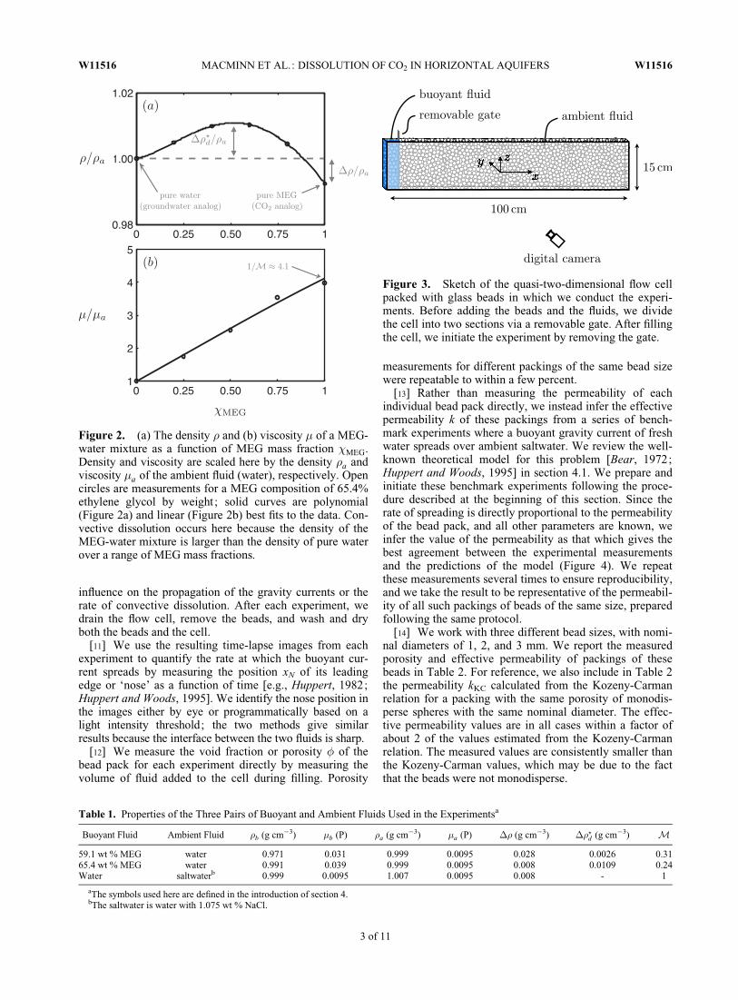
[7] We conduct experiments with water and solutions ofmethanol and ethylene glycol (MEG) [Turner and Yang,1963; Turner, 1966; Huppert et al., 1986]. MEG solutionswith ethylene glycol mass fractions less than about 0.68 areless dense than water, so such MEG solutions play the roleof the buoyant CO2 while water plays the role of the rela-tively dense, ambient groundwater [Neufeld et al., 2010]. Abuoyant gravity current of MEG spreading over water issubject to convective dissolution because the density ofMEG-water mixtures is a nonmonotonic function of MEGmass fraction, and is larger than that of either MEG orwater over a range of mass fractions. As a result, the densemixture of MEG and water that forms along their sharedinterface drives convective dissolution.

[8] The rate at which a buoyant current of MEG spreadsover water is directly proportional to the amount by whichthe density of the water exceeds the density of the MEG.The rate at which a buoyant current of MEG dissolves intowater by convective dissolution scales with the amount bywhich the maximum density of a MEG-water mixtureexceeds the density of water. We denote the former densitydifference by �� and the latter by ��?d (Figure 2). A con-venient aspect of the MEG-water system is that these tworates can be adjusted relative to one another via the ratio ofmethanol to ethylene glycol in the pure MEG. Increasingthe initial mass fraction of ethylene glycol decreases ��but increases ��?d , leading to slower spreading but fasterconvective dissolution. Here, we work with two differentMEG compositions: 59.1% and 65.4% ethylene glycolby mass, hereafter referred to as ‘‘59.1 wt % MEG’’ and‘‘65.4 wt % MEG,’’ respectively. The latter spreads moreslowly but dissolves more quickly than the former. We reportthe key properties of these two MEG mixtures in Table 1.

[9] Although MEG and water are perfectly miscible,unlike CO2 and water, mixing due to diffusion and disper-sion is slow in this system and the initially sharp ‘‘inter-face’’ between the two fluids is preserved over the durationof the experiment.

2.2. Flow Cell

[10] We conduct the experiments in a quasi-two-dimensional flow cell packed with spherical glass beads(Figure 3). The cell is 100 cm long and 15 cm tall, with a1 cm gap between the plates. The cell is open at the top.We initially divide the cell into two sections via a remov-able gate, inserted 9 cm from the left edge. After packingboth sections with beads following a consistent protocol,we add the buoyant fluid to the smaller, left section and theambient fluid to the larger, right section. To initiate theexperiment, we remove the gate and record the resultingfluid flow with a digital camera. Removal of the gate causessome local bead rearrangement, but this occurs on a muchshorter timescale than the flow and has no discernible

Figure 1. A sketch of the simple model problem consideredhere: a buoyant gravity current (dark blue) spreads beneath ahorizontal caprock in a vertically confined aquifer, shrinkingas the buoyant fluid dissolves into the ambient fluid via con-vective dissolution (light blue).

W11516 MACMINN ET AL.: DISSOLUTION OF CO2 IN HORIZONTAL AQUIFERS W11516

2 of 11

influence on the propagation of the gravity currents or therate of convective dissolution. After each experiment, wedrain the flow cell, remove the beads, and wash and dryboth the beads and the cell.

[11] We use the resulting time-lapse images from eachexperiment to quantify the rate at which the buoyant cur-rent spreads by measuring the position xN of its leadingedge or ‘nose’ as a function of time [e.g., Huppert, 1982;Huppert and Woods, 1995]. We identify the nose position inthe images either by eye or programmatically based on alight intensity threshold; the two methods give similarresults because the interface between the two fluids is sharp.

[12] We measure the void fraction or porosity � of thebead pack for each experiment directly by measuring thevolume of fluid added to the cell during filling. Porosity

measurements for different packings of the same bead sizewere repeatable to within a few percent.

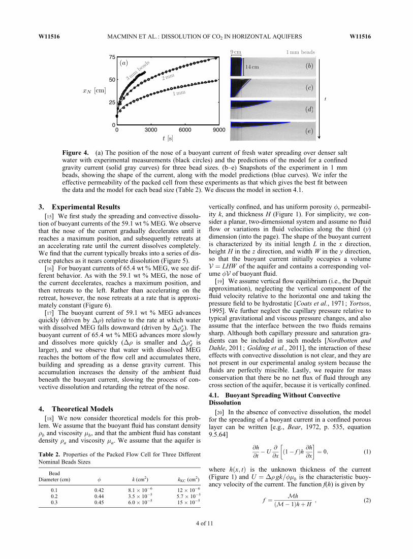
[13] Rather than measuring the permeability of eachindividual bead pack directly, we instead infer the effectivepermeability k of these packings from a series of bench-mark experiments where a buoyant gravity current of freshwater spreads over ambient saltwater. We review the well-known theoretical model for this problem [Bear, 1972;Huppert and Woods, 1995] in section 4.1. We prepare andinitiate these benchmark experiments following the proce-dure described at the beginning of this section. Since therate of spreading is directly proportional to the permeabilityof the bead pack, and all other parameters are known, weinfer the value of the permeability as that which gives thebest agreement between the experimental measurementsand the predictions of the model (Figure 4). We repeatthese measurements several times to ensure reproducibility,and we take the result to be representative of the permeabil-ity of all such packings of beads of the same size, preparedfollowing the same protocol.

[14] We work with three different bead sizes, with nomi-nal diameters of 1, 2, and 3 mm. We report the measuredporosity and effective permeability of packings of thesebeads in Table 2. For reference, we also include in Table 2the permeability kKC calculated from the Kozeny-Carmanrelation for a packing with the same porosity of monodis-perse spheres with the same nominal diameter. The effec-tive permeability values are in all cases within a factor ofabout 2 of the values estimated from the Kozeny-Carmanrelation. The measured values are consistently smaller thanthe Kozeny-Carman values, which may be due to the factthat the beads were not monodisperse.

Figure 2. (a) The density � and (b) viscosity � of a MEG-water mixture as a function of MEG mass fraction �MEG.Density and viscosity are scaled here by the density �a andviscosity �a of the ambient fluid (water), respectively. Opencircles are measurements for a MEG composition of 65.4%ethylene glycol by weight; solid curves are polynomial(Figure 2a) and linear (Figure 2b) best fits to the data. Con-vective dissolution occurs here because the density of theMEG-water mixture is larger than the density of pure waterover a range of MEG mass fractions.

Table 1. Properties of the Three Pairs of Buoyant and Ambient Fluids Used in the Experimentsa

Buoyant Fluid Ambient Fluid �b (g cm�3) �b (P) �a (g cm�3) �a (P) �� (g cm�3) ��?d (g cm�3) M

59.1 wt % MEG water 0.971 0.031 0.999 0.0095 0.028 0.0026 0.3165.4 wt % MEG water 0.991 0.039 0.999 0.0095 0.008 0.0109 0.24Water saltwaterb 0.999 0.0095 1.007 0.0095 0.008 - 1

aThe symbols used here are defined in the introduction of section 4.bThe saltwater is water with 1.075 wt % NaCl.

Figure 3. Sketch of the quasi-two-dimensional flow cellpacked with glass beads in which we conduct the experi-ments. Before adding the beads and the fluids, we dividethe cell into two sections via a removable gate. After fillingthe cell, we initiate the experiment by removing the gate.


3 of 11

3. Experimental Results[15] We first study the spreading and convective dissolu-

tion of buoyant currents of the 59.1 wt % MEG. We observethat the nose of the current gradually decelerates until itreaches a maximum position, and subsequently retreats atan accelerating rate until the current dissolves completely.We find that the current typically breaks into a series of dis-crete patches as it nears complete dissolution (Figure 5).

[16] For buoyant currents of 65.4 wt % MEG, we see dif-ferent behavior. As with the 59.1 wt % MEG, the nose ofthe current decelerates, reaches a maximum position, andthen retreats to the left. Rather than accelerating on theretreat, however, the nose retreats at a rate that is approxi-mately constant (Figure 6).

[17] The buoyant current of 59.1 wt % MEG advancesquickly (driven by ��) relative to the rate at which waterwith dissolved MEG falls downward (driven by ��?d). Thebuoyant current of 65.4 wt % MEG advances more slowlyand dissolves more quickly (�� is smaller and ��?d islarger), and we observe that water with dissolved MEGreaches the bottom of the flow cell and accumulates there,building and spreading as a dense gravity current. Thisaccumulation increases the density of the ambient fluidbeneath the buoyant current, slowing the process of con-vective dissolution and retarding the retreat of the nose.

4. Theoretical Models[18] We now consider theoretical models for this prob-

lem. We assume that the buoyant fluid has constant density�b and viscosity �b, and that the ambient fluid has constantdensity �a and viscosity �a. We assume that the aquifer is

vertically confined, and has uniform porosity �, permeabil-ity k, and thickness H (Figure 1). For simplicity, we con-sider a planar, two-dimensional system and assume no fluidflow or variations in fluid velocities along the third (y)dimension (into the page). The shape of the buoyant currentis characterized by its initial length L in the x direction,height H in the z direction, and width W in the y direction,so that the buoyant current initially occupies a volumeV ¼ LHW of the aquifer and contains a corresponding vol-ume �V of buoyant fluid.

[19] We assume vertical flow equilibrium (i.e., the Dupuitapproximation), neglecting the vertical component of thefluid velocity relative to the horizontal one and taking thepressure field to be hydrostatic [Coats et al., 1971; Yortsos,1995]. We further neglect the capillary pressure relative totypical gravitational and viscous pressure changes, and alsoassume that the interface between the two fluids remainssharp. Although both capillary pressure and saturation gra-dients can be included in such models [Nordbotten andDahle, 2011; Golding et al., 2011], the interaction of theseeffects with convective dissolution is not clear, and they arenot present in our experimental analog system because thefluids are perfectly miscible. Lastly, we require for massconservation that there be no net flux of fluid through anycross section of the aquifer, because it is vertically confined.

4.1. Buoyant Spreading Without ConvectiveDissolution

[20] In the absence of convective dissolution, the modelfor the spreading of a buoyant current in a confined porouslayer can be written [e.g., Bear, 1972, p. 535, equation9.5.64]

@h

@t� U

@

@xð1� f Þh @h

@x

� �¼ 0; (1)

where hðx; tÞ is the unknown thickness of the current(Figure 1) and U ¼ �� gk=��b is the characteristic buoy-ancy velocity of the current. The function f(h) is given by

f ¼ Mh

ðM� 1Þhþ H; (2)

Figure 4. (a) The position of the nose of a buoyant current of fresh water spreading over denser saltwater with experimental measurements (black circles) and the predictions of the model for a confinedgravity current (solid gray curves) for three bead sizes. (b–e) Snapshots of the experiment in 1 mmbeads, showing the shape of the current, along with the model predictions (blue curves). We infer theeffective permeability of the packed cell from these experiments as that which gives the best fit betweenthe data and the model for each bead size (Table 2). We discuss the model in section 4.1.

Table 2. Properties of the Packed Flow Cell for Three DifferentNominal Beads Sizes

BeadDiameter (cm) � k (cm2) kKC (cm2)

0.1 0.42 8.1 � 10�6 12 � 10�6

0.2 0.44 3.5 � 10�5 5.7 � 10�5

0.3 0.45 6.0 � 10�5 15 � 10�5


4 of 11

with mobility ratio M¼ �a=�b. The presence of f(h)reflects the fact that the aquifer is vertically confined, sothat the buoyant fluid must displace the relatively viscousambient fluid in order to spread. Flow of the ambient fluidbecomes unimportant at late times as the current becomesthin relative to the aquifer thickness (f ðhÞ � 1 whenh� H). The spreading behavior becomes independent ofM in this unconfined limit [Barenblatt, 1996; Hesse et al.,2007].

[21] To rewrite equation (1) in dimensionless form, wedefine scaled variables

~h ¼ h

H; ~t ¼ UH

L2t ; ~x ¼ x

L; (3)

and obtain

@~h

@~t� @

@~xð1� f Þ~h @

~h

@~x

" #¼ 0: (4)

In the unconfined limit, equation (4) has a similarity solu-tion from Barenblatt [1952],

~hð~x;~tÞ ¼ 1

6~t�1=3

92=3 � ~x2

~t2=3

� �; (5)

valid for j~xj � ~xN ð~tÞ and ~t > 0. Equation (5) indicates thatthe position ~xN of the nose of an unconfined current willincrease monotonically in time according to the power law

~xN ð~tÞ ¼ ð9~tÞ1=3: (6)

The solution to equation (4) will converge to equation (5)as the current becomes thin for any initial shape with com-pact support. The convergence time is small for M� 1and increases strongly with M [Hesse et al., 2007;MacMinn and Juanes, 2009].

[22] We compare the predictions of equation (4) withbenchmark experiments in which buoyant water spreads

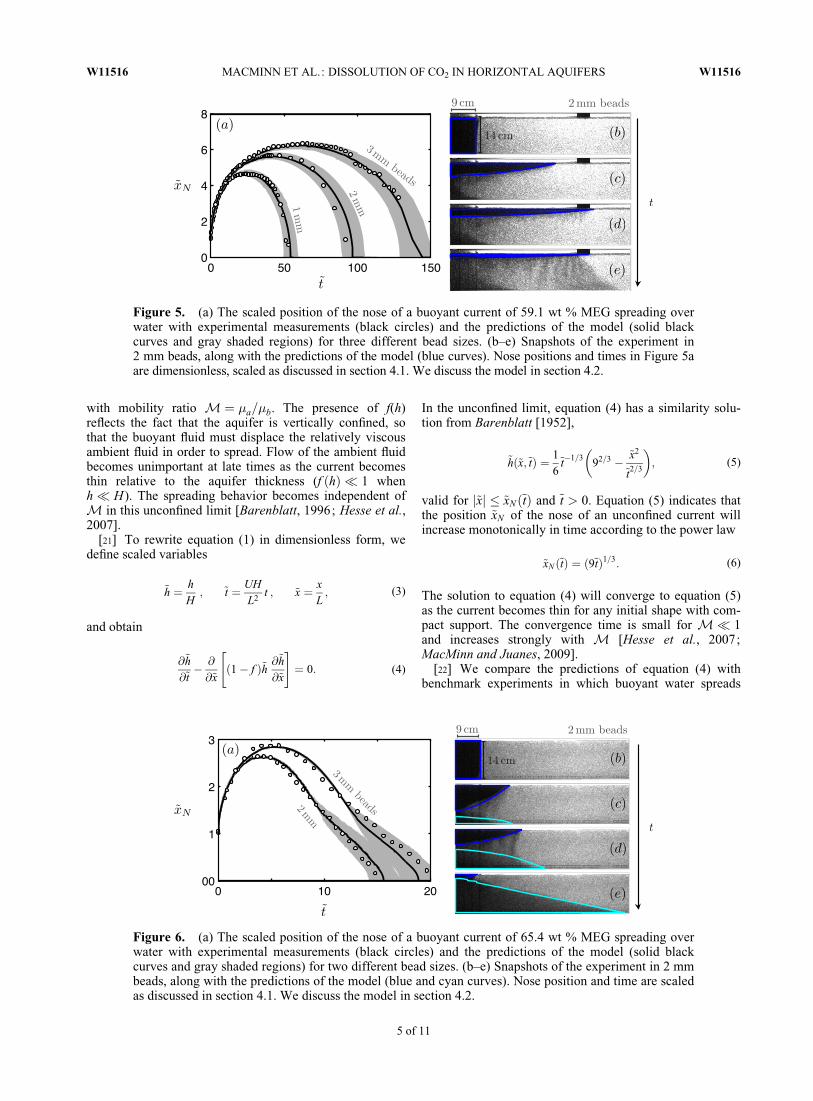
Figure 5. (a) The scaled position of the nose of a buoyant current of 59.1 wt % MEG spreading overwater with experimental measurements (black circles) and the predictions of the model (solid blackcurves and gray shaded regions) for three different bead sizes. (b–e) Snapshots of the experiment in2 mm beads, along with the predictions of the model (blue curves). Nose positions and times in Figure 5aare dimensionless, scaled as discussed in section 4.1. We discuss the model in section 4.2.

Figure 6. (a) The scaled position of the nose of a buoyant current of 65.4 wt % MEG spreading overwater with experimental measurements (black circles) and the predictions of the model (solid blackcurves and gray shaded regions) for two different bead sizes. (b–e) Snapshots of the experiment in 2 mmbeads, along with the predictions of the model (blue and cyan curves). Nose position and time are scaledas discussed in section 4.1. We discuss the model in section 4.2.


5 of 11

over ambient saltwater (Figure 4). The ambient saltwatercontains 1:075 % NaCl by weight, so the driving densitydifference is �� ¼ 7:52 kg m�3 and the mobility ratio isM¼ 1 (Table 1). As discussed in section 2.2, we use theseexperiments to infer the effective permeability of the flow cell.

4.2. Buoyant Spreading With Convective Dissolution

[23] Previous studies of convective dissolution haveshown that a stationary layer of CO2 will dissolve into asemi-infinite layer of water at a rate that is roughly constantin time [Hidalgo and Carrera, 2009; Kneafsey and Pruess,2010; Pau et al., 2010]. When the water layer has a finitethickness, recent results suggest that the dissolution rate isa weak function of the layer thickness [Neufeld et al.,2010; Backhaus et al., 2011], but that it can be approxi-mated as constant provided that the thickness of the CO2

layer is small relative to the thickness of the water layer.[24] An upscaled model for convective dissolution can

then be incorporated into models such as equation (1) byintroducing a constant loss or sink term [Gasda et al.,2011; MacMinn et al., 2011],

@h

@t� U

@

@xð1� f Þh @h

@x

� �¼ � qd

�; (7)

where the dissolution rate qd is the volume of buoyant fluidthat dissolves per unit bulk fluid-fluid interfacial area perunit time. Rewriting equation (7) in dimensionless formusing (3), we obtain

@~h

@~t� @

@~xð1� f Þ~h @

~h

@~x

" #¼ ��; (8)

where

� ¼ L

H

� �2 qd

�U(9)

is the dimensionless dissolution rate. Pritchard et al. [2001]studied equation (8) in the unconfined limit (f ¼ 0) in a dif-ferent context, developing the explicit solution

~hð~x;~tÞ ¼ 1

6~t�1=3

92=3 � ~x2

~t2=3

� �� 3

4�~t; (10)

valid for j~xj � ~xN ð~tÞ and ~t > 0. As discussed by Pritchardet al. [2001], equation (10) implies that the position of thenose of the current evolves according to

~xN ð~tÞ ¼ ð9~tÞ1=3

ffiffiffiffiffiffiffiffiffiffiffiffiffiffiffiffiffiffiffiffiffiffiffiffiffiffiffiffiffiffiffi1� 1

18� ð9~tÞ4=3

r: (11)

Equations (10) and (11) reduce to equations (5) and (6),respectively, when � ¼ 0:

[25] Equation (11) predicts that convective dissolution willhave a strong impact on the spreading of the current in theunconfined limit. Without convective dissolution ð� ¼ 0Þ, thenose of the current advances for all time following the powerlaw xN / t1=3 (equation 6). With convective dissolution, thenose reaches a maximum position ~xmax

N ¼ ð8=3Þ1=4��1=4 and

then retreats to the origin as the volume of the currentdecreases to zero at time ~t

end ¼ ð8=9Þ1=4��3=4 (Figure 7a).We refer to this time ~t

endas the ‘lifetime’ of the current.

[26] The spreading behavior for nonnegligible M isqualitatively similar to the unconfined behavior predictedby equations (6) and (11), but the current spreads moreslowly asM increases (Figure 7b). Accordingly, the maxi-mum extent of the current decreases withM while the life-time of the current increases with M. However, thescalings of these quantities with � show only minor devia-tions from the unconfined predictions of ~xmax

N � ��1=4 and~t

end � ��3=4 (Figure 8).[27] Equation (10) is not strictly an asymptotic solution

of equation (8) because convective dissolution causes somememory of the initial shape to be retained throughout theevolution, as with residual trapping [Kochina et al., 1983;Barenblatt, 1996]. In addition, the concept of asymptoticshas limited relevance here because the current dissolvescompletely in finite time.

[28] The predictions of equation (8) are in qualitativeagreement with our experimental observations for currentsof the faster-spreading, slower-dissolving MEG (59.1 wt %).Quantitative comparison requires an estimate of the dissolu-tion rate qd. Expressions for qd for a stationary layer havebeen presented by Pau et al. [2010] and Neufeld et al.[2010]. The latter, in particular, performed experiments withthe same pair of analog fluids used here. Based on those

Figure 7. (a) Dimensionless nose position against dimen-sionless time for an unconfined gravity current (i.e., forM� 1), as determined from equations (6) and (11) forseveral values of the dimensionless dissolution rate �. (b)Dimensionless nose position against dimensionless time fora confined gravity current (i.e., for nonnegligible M), asdetermined from numerical solutions to the confined model(equation (8)) for several values ofM at fixed � ¼ 0:003.


6 of 11

results in conjunction with high-resolution numerical simula-tions, Neufeld et al. [2010] suggested that

qd ¼ b��?vD

H

� ��?d gkH

��aD

� �n

; (12)

where �?v ¼ �?d�?m=�b measures the volume of buoyant fluiddissolved in one unit volume of ambient fluid containingthe maximum (saturated) mass fraction �?m of dissolvedbuoyant fluid, D � 1� 10�5 cm2 is the molecular diffusiv-ity of aqueous buoyant fluid in a porous medium, andb � 0:12 and n � 0:84 are dimensionless constants.Although the characteristic vertical scale here should be thedepth of the layer of ambient fluid below the buoyant cur-rent, we use the total depth of the fluid layer H � 14 cm forsimplicity since the buoyant current is thin for most ofits evolution ðh� HÞ. Dissolution due to diffusion anddispersion are not included in this estimate of qd sincethese are negligible compared to convective dissolution[Ennis-King et al., 2005].

[29] We begin by estimating the dissolution rate fromthis expression for 59.1 wt % MEG dissolving into water.We then treat the dissolution rate as a fitting parameter, cal-ibrating its value around this estimate by comparing thepredictions of the model with experimental measurements.We present the estimated and calibrated dissolution rates,

qestd and qd, respectively, in Table 3. The calibrated values

are within about a factor of two of the estimated values.That they do not agree exactly is not surprising, given thatthe correlation of Neufeld et al. [2010] was developed inthe context of a stationary layer of MEG dissolving intowater. Diffusion and flow-induced dispersion in the presentcontext, where the interface has both advancing and reced-ing portions, may enhance or inhibit convective dissolutionrelative to the case of a stationary layer.

[30] We compare these experiments with the predictionsof equation (8) in Figure 5. We compare the evolution ofthe nose position for all three bead sizes, as well as the evo-lution of the shape of the current for the 2 mm beads. Weinclude an envelope around the nose position correspond-ing to 610 % around the calibrated dissolution rate qd toillustrate the sensitivity of the model to this parameter.

[31] These results suggest that the assumption of a con-stant rate of convective dissolution can capture the qualita-tive and quantitative features of the impact of convectivedissolution on a buoyant current in this system, providedthat dissolved buoyant fluid accumulates slowly beneaththe buoyant current.

5. Two-Current Model for Spreading WithConvective Dissolution

[32] Experimental and numerical studies of convectivedissolution have thus far focused on dissolution from a sta-tionary layer of CO2 overlying a deep or semi-infinite layerof water. In a confined aquifer, we expect that the accumu-lation of dissolved CO2 in the water beneath the buoyantcurrent will limit the rate at which the CO2 can dissolve.Here, we extend the model discussed above (equation (8))to include this accumulation effect in a simple way.

[33] In our experiments with buoyant currents of slower-spreading, faster-dissolving MEG (65.4 wt %), weobserved that the accumulation of dissolved MEG in thewater played a strong role in the dynamics of the buoyantcurrent. In particular, water with dissolved MEG accumu-lated on the bottom of the aquifer and slumped downwardrelative to the ambient fluid because of its larger density.Although the details of convective dissolution and subse-quent mass transport are complex, we develop a simplemodel for this process by assuming that it primarily trans-ports dissolved buoyant fluid vertically from the buoyantcurrent down to a dense current of ambient fluid with dis-solved buoyant fluid (Figure 9). We assume that this densecurrent consists of ambient fluid with a constant and uni-form mass fraction �m of dissolved buoyant fluid, with cor-responding density �d and viscosity �d , and we denote itsunknown local thickness by hdðx; tÞ. Note that �m may beless than the maximum (saturated) mass fraction �?m. We

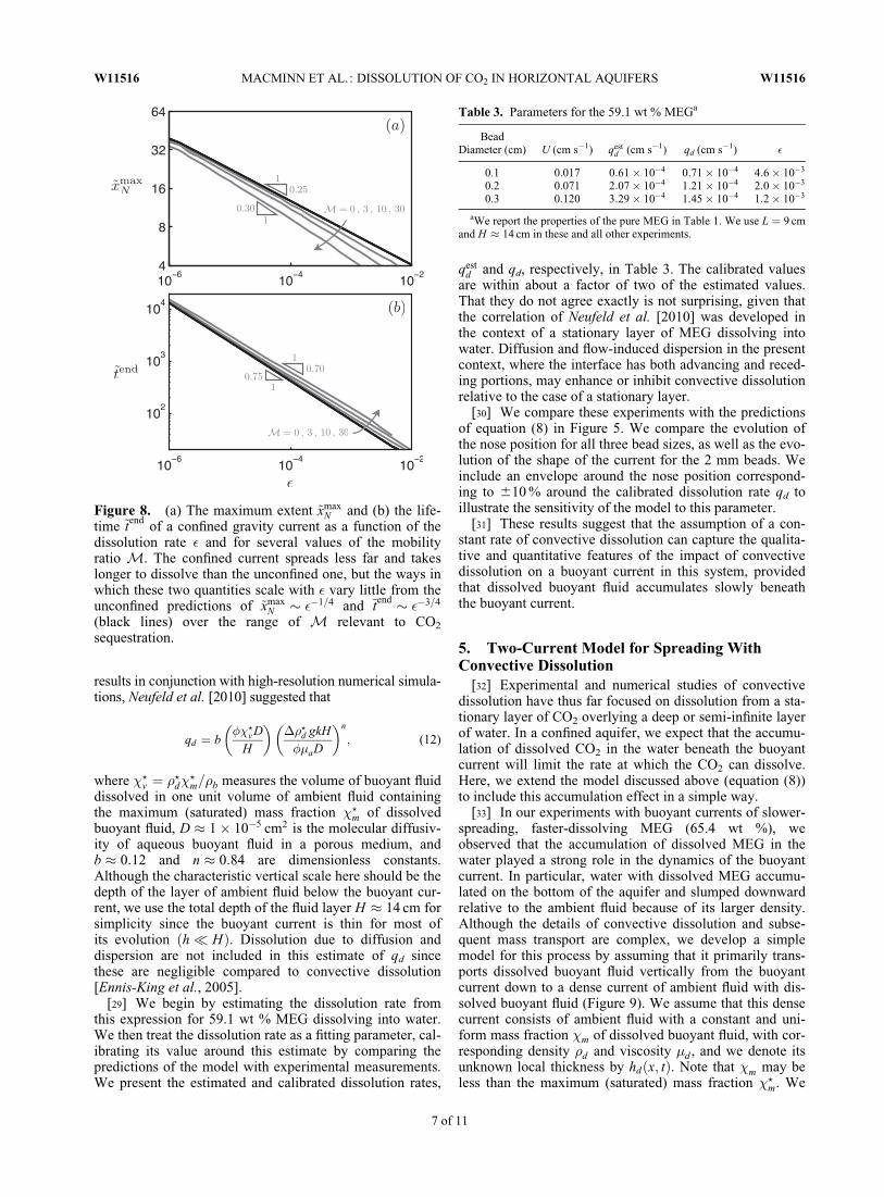
Figure 8. (a) The maximum extent ~xmaxN and (b) the life-

time ~tend

of a confined gravity current as a function of thedissolution rate � and for several values of the mobilityratio M. The confined current spreads less far and takeslonger to dissolve than the unconfined one, but the ways inwhich these two quantities scale with � vary little from theunconfined predictions of ~xmax

N � ��1=4 and ~tend � ��3=4

(black lines) over the range of M relevant to CO2

sequestration.

Table 3. Parameters for the 59.1 wt % MEGa

BeadDiameter (cm) U (cm s�1) qest

d (cm s�1) qd (cm s�1) �

0.1 0.017 0:61� 10�4 0:71� 10�4 4:6� 10�3

0.2 0.071 2:07� 10�4 1:21� 10�4 2:0� 10�3

0.3 0.120 3:29� 10�4 1:45� 10�4 1:2� 10�3

aWe report the properties of the pure MEG in Table 1. We use L ¼ 9 cmand H � 14 cm in these and all other experiments.


7 of 11

assume that convective dissolution transfers fluid from thebuoyant current to the dense current at a constant rateexcept where the ambient fluid is locally saturated, whichwe assume occurs where the buoyant current and the densecurrent touch (hþ hd ¼ 1). For simplicity, we assume thatbuoyant fluid accumulates in the dense current at the sameposition x and time t at which it dissolved from the buoyantcurrent.

[34] Applying Darcy’s law and conservation of mass forthis system, and assuming sharp interfaces and verticalflow equilibrium as discussed at the beginning of section 4above, we have in dimensionless form

@~h

@~t� @

@~xð1� f Þ~h @

~h

@~x� �f ~hd

@~hd

@~x

" #¼ �~� (13)

@~hd

@~t� @

@~x�ð1� fdÞ~hd

@~hd

@~x� fd

~h@~h

@~x

" #¼ ~�

�v

; (14)

where ~h, ~x, and ~t are as defined in equation (3). The nonlinearfunction f now includes the presence of the dense current,

f ¼ Mh

ðM� 1Þhþ ðMd � 1Þhd þ 1(15)

and we have a second such function

fd ¼Mdhd

ðM� 1Þhþ ðMd � 1Þhd þ 1: (16)

Finally, we redefine the dimensionless convective dissolu-tion rate � to be conditional,

� ¼ðL=HÞ2 ðqd=�UÞ if hþ hd < 1;

0 if hþ hd ¼ 1;

((17)

so that it takes a constant, nonzero value where the buoyantcurrent and the dense one are separate and vanishes wherethey are touching.

[35] This two-current model contains three new parame-ters relative to the simpler model: Md ¼ �a=�d , which isthe ratio of the viscosity of the ambient fluid, �a, to that ofthe dense mixture, �d ; � ¼ Ud=U ¼ ð��d=�dÞ=ð��=�bÞ,which is the ratio of the characteristic buoyancy velocity ofthe dense current, Ud ¼ ð�d � �aÞgk=��d , to that of thebuoyant one, U ; and �v ¼ �d�m=�b � �?v , which is the vol-ume fraction of buoyant fluid dissolved in the dense currentat mass fraction �m. All three of these parameters areuniquely defined by the properties of the buoyant and ambi-ent fluids, the value of �m, and appropriate constitutiverelations �dð�Þ and �dð�Þ for the mixture.

[36] The buoyant current loses volume due to convectivedissolution at a rate � per unit length, and this volume istransferred to the dense current at a rate �=�v per unitlength. This model reduces to the simpler model (equation(8)) for �v !1, when one unit volume of the dense cur-rent can hold an arbitrary amount of dissolved buoyantfluid so that the dense current does not accumulate no mat-ter how much buoyant fluid dissolves.

[37] We solve equations (13) and (14) numerically. Todo so, we discretize the two equations in space using a sec-ond-order finite-volume method to guarantee conservationof volume. We then integrate the two equations in timeusing a first-order explicit method, which greatly simplifiesthe handling of the coupling between these two nonlinearconservation laws. Explicit time integration requires small,local corrections to the mass transfer between the two cur-rents at the end of each time step in order to avoid local over-shoot where the dense current rises to meet the buoyant one.

[38] We find that the accumulation of the dense currentstrongly inhibits convective dissolution from the buoyantcurrent, leading to a marked departure from the behaviorpredicted by the single-current model when the two cur-rents touch (Figure 10).

[39] The predictions of this model are in qualitative agree-ment with our experimental observations for the slower-spreading, faster-dissolving MEG (65.4 wt %). Quantitativecomparison requires an estimate of the dissolution rate qd

and the mass fraction �m of dissolved MEG in the lowerlayer. As discussed above, the parameters �v, Md, and � arethen calculated from �m based on the constitutive relationsfor MEG-water mixtures (Figure 2).

[40] We again estimate qd from equation (12), and thencalibrate qd around this estimated value in order to matchthe early time spreading behavior, during which time thedense current plays little role. We develop an initial estimateof the mass fraction �m of MEG in the dense current basedon the final volume of the dense current once the buoyantcurrent has completely dissolved, and we then calibrate �maround this value. We report these values in Table 4.

[41] We compare the predictions of this model with ourexperiments with the slower-spreading, faster-dissolvingMEG (65.4 wt %) in Figure 6. We compare the evolutionof the nose position for two bead sizes, as well as the evolu-tion of the shape of the buoyant current for the 2 mm beads.We include an envelope around the nose position corre-sponding to 65 % around the calibrated mass fraction �m.The nose position is quite sensitive to this quantity since

Figure 9. A sketch of the two-current model where dis-solved buoyant fluid accumulates in a dense gravity current(light blue) that grows and spreads along the bottom of theaquifer as the buoyant current (dark blue) shrinks andspreads along the top.


8 of 11

varying it here changes the time at which the two currentstouch and the subsequent rate of retreat (Figure 10b), andalso the properties of the dense current via the parameters �andMd .

[42] These results suggest that this model captures thefundamental impact of the accumulation of dissolved buoy-ant fluid in the ambient water. However, one limitation ofthis model is that we do not have an a priori estimate of themass fraction �m, and the model is very sensitive to thisquantity. To develop such an estimate will require furtherexperiments and high-resolution numerical simulations tostudy the accumulation of dissolved buoyant fluid. Also,although we have assumed that convective dissolution

ceases locally when the two currents touch, the fact that �mis less than the maximum value �?m implies that convectivedissolution may continue at a reduced rate after the twocurrents touch since it remains possible to generate mix-tures at the interface that are denser than the surroundingfluid. The comparison between this model and our experi-mental results implies that this model captures the funda-mental behavior of the MEG-water system, but furtherstudy will be necessary to assess the limits of this model inpractice.

6. Application to Carbon Sequestration[43] We now consider these results in the context of

CO2 sequestration in a saline aquifer. A key differencebetween the MEG-water system and the CO2-water systemis that MEG and water are fully miscible, whereas CO2 andwater are immiscible. Although the impact of capillarity onconvective dissolution is unknown, it has been shown thatthe impact of capillarity on the spreading of a gravity cur-rent is negligible when the capillary pressure is small rela-tive to typical gravitational and viscous pressure changes[Nordbotten and Dahle, 2011; Golding et al., 2011]. Weassume that this is also the case for convective dissolution.We next compare the dimensionless parameters for theCO2-water system with those for the MEG-water system.

[44] Motivated by the Sleipner site in the North Sea,we consider an aquifer for which �b � 500 kg m�3, �b �4� 10�5 Pa s, �a � 1000 kg m�3, and �a � 6� 10�4 Pa s[Bickle et al., 2007], giving a mobility ratio of M� 15.This value of M is much larger than in the MEG-watersystem (M� 0:31 for the 59.11 wt % MEG and � 0.24for the 65.4 wt % MEG). As a result, the CO2 plume willbe much more strongly tongued than the MEG plume,presenting much more interfacial area for convective disso-lution and increasing its effectiveness [MacMinn et al.,2011].

[45] For an aquifer of thickness H � 20 m, porosity� � 0:375, and permeability k � 2:5� 10�12 m2, the char-acteristic spreading rate of the CO2 plume is U �5:8� 10�5 m s�1 and Neufeld et al. [2010] estimated thedissolution rate to be qd � 1� 10�9 m s�1. The estimate ofPau et al. [2010] for the dissolution rate in the Carrizo-Wilcox aquifer in Texas is of the same order. For a rela-tively large sequestration project in such an aquifer, whereM � 10 Mt of CO2 is injected along a linear array of wells[Nicot, 2008] of length W � 10 km, the characteristiclength is L ¼ M=2�b�HW � 130 m and the correspondingdimensionless dissolution rate is � ¼ qdL2=�UH2 � 0:002.Although quite sensitive to the specific injection scenario,this value is comparable to the values from our experiments

Figure 10. (a) The evolution of the nose of the buoyantcurrent from numerical solutions to the two-current modelfor several values of � without (dashed black lines) andwith (solid gray lines) accumulation. The presence of thedense current retards the nose of the buoyant currentweakly due to hydrodynamic interactions before the twocurrents touch and then strongly by inhibiting convectivedissolution after the two currents touch (M¼ 0:25,Md ¼ 1, � ¼ 1:1, �v ¼ 0:2). (b) Solutions for � ¼ 0:01and several values of �v (other parameters unchanged). Thetwo currents touch earlier as �v decreases, and the noseretreats more slowly thereafter.

Table 4. Parameters for the 65.4 wt % MEGa

BeadDiameter (cm) U (cm s�1) qest

d (cm s�1) qd (cm s�1) � �v Md �

0.1 3:6� 10�3 2:0� 10�4 1:8� 10�4 0.055 0.30 0.51 2.140.2 1:5� 10�2 6:8� 10�4 6:8� 10�4 0.040 0.30 0.51 2.140.3 2:5� 10�2 1:1� 10�3 8:2� 10�4 0.028 0.28 0.53 2.06

aWe report the properties of the pure MEG in Table 1. We use L ¼ 9 cm and H � 14 cm in these and all other experiments. Here �m and �v are approx-imately equal.


9 of 11

(� � 0.001–0.005 for the 59.11 wt % MEG and � 0.03–0.06for the 65.4 wt % MEG).

[46] Unlike in our experiments, the solubility of CO2 ingroundwater is only a few percent by weight at typical aq-uifer conditions [Duan and Sun, 2003]. For �m � 0:01, thecorresponding increase in the density of the water is��d � 10 kg m�3 [Garc�ıa, 2001] and the change in its vis-cosity is negligible, so we expect �v � 0:02, � � 0:02, andMd � 1. These values of �v and � are about an order ofmagnitude smaller than those in our experiments.

[47] Based on these values of �, �, and �v, we expect dis-solved CO2 to accumulate very quickly and slump down-ward very slowly relative to the rate at which the buoyantcurrent spreads. As a result, we expect the rate at whichCO2 is trapped to be controlled not by the rate of convec-tive dissolution, but by the amount of dissolved CO2 thewater can hold (i.e., �v) and by the rate at which this waterslumps downward. In Figure 11, we show that this is indeedthe case: both the maximum extent and the lifetime of aplume of CO2 decrease as the dissolution rate increases,but both quantities approach limiting values that are inde-pendent of the dissolution rate if this rate is sufficientlylarge. The dissolution rate of � � 0:002 estimated above isabout 2 orders of magnitude above this threshold value. Asa result, the spreading and convective dissolution of the

plume is completely controlled by the accumulation ofdissolved CO2 in this setting, and the plume spreads severaltimes further and persists for several orders of magnitudelonger than it would without this accumulation.

7. Discussion and Conclusions[48] We have shown via experiments with analog fluids

that simple models are able to capture the impact of con-vective dissolution on the spreading of a buoyant gravitycurrent in a vertically confined, horizontal layer.

[49] When dissolved buoyant fluid accumulates slowlybeneath the buoyant current, our experiments have con-firmed that the complex dynamics of convective dissolutioncan be upscaled to a constant mass flux [Pau et al., 2010;Kneafsey and Pruess, 2010; Neufeld et al., 2010] andincorporated into a simple model [Gasda et al., 2011;MacMinn et al., 2011] (Figure 5).

[50] When dissolved buoyant fluid accumulates quicklybeneath the buoyant current, our experiments have shownthat this accumulation can have an important limiting effecton the dissolution process. To capture the accumulation ofdissolved buoyant fluid, we have developed a two-currentmodel where a dense gravity current of ambient fluid withdissolved buoyant fluid grows and spreads along the bottomof the aquifer. We have used this model to show that theaccumulation of dissolved buoyant fluid beneath the buoy-ant current can slow convective dissolution, and we haveconfirmed this prediction experimentally (Figure 6).

[51] Using this two-current model, we have shown thatwe expect CO2 spreading and dissolution in a horizontalaquifer to be controlled primarily by the mass fraction atwhich CO2 accumulates in the water, and to be nearly inde-pendent of the dissolution rate (Figure 11). This can be thecase even in the presence of aquifer slope or backgroundgroundwater flow, both of which drive net CO2 migrationand expose the plume to fresh water, when slope- or flow-driven migration is sufficiently slow [MacMinn et al.,2011].

[52] The planar models used here rely on the fact that thetransverse width of the buoyant current is much larger than itslength in the x direction, W � L, which is typically the casewhen large amounts of CO2 are injected via a line drive con-figuration [Nicot, 2008; Szulczewski et al., 2012]. The modelspresented here can be readily adapted to a radial geometry forinjection from a single well where appropriate. Where neithergeometric approximation is appropriate, use of a more com-plicated, two-dimensional model will be necessary.

[53] We have also assumed here an idealized rectangularinitial shape for the plume of CO2. In practice, the specificdetails of the injection scenario will have some quantitativeimpact on the maximum extent and lifetime of the CO2, butshould have little qualitative impact on the interactionbetween plume spreading, convective dissolution, and theaccumulation of dissolved CO2.

[54] Acknowledgments. C.W.M. gratefully acknowledges the supportof a David Crighton Fellowship and a Yale Climate and Energy InstitutePostdoctoral Fellowship. J.A.N. is supported by a Royal Society UniversityResearch Fellowship. The work of H.E.H. is partially supported by a RoyalSociety Wolfson Research Merit Award. M.A.H. acknowledges support bythe U.S. Department of Energy’s National Energy Technology Laboratoryunder DE-FE0001563. The views expressed herein do not necessarilyreflect those of the U.S. government or any agency thereof.

Figure 11. (a) The maximum extent xmaxN and (b) the life-

time tend of a buoyant plume of CO2 spreading in a salineaquifer as a function of the dissolution rate � in the uncon-fined limit (solid black curve), from a numerical solution ofequation (8) (dashed black curve), and from a numerical so-lution of the two-layer model (dash-dotted gray curve). Wealso show in Figure 11a the position of the nose of thedense current at time tend (dotted blue curve). Parametersare appropriate for the Sleipner formation, as discussed insection 6.


10 of 11

ReferencesBackhaus, S., K. Turitsyn, and R. E. Ecke (2011), Convective instability

and mass transport of diffusion layers in a Hele-Shaw geometry, Phys.Rev. Lett., 106(10), 104501.

Barenblatt, G. I. (1952), On some unsteady motions of fluids and gases in aporous medium [in Russian], Appl. Math. Mech., 16(1), 67–78.

Barenblatt, G. I. (1996), Scaling, Self-Similarity, and Intermediate Asymp-totics, Cambridge Univ. Press, Cambridge, U. K.

Bear, J. (1972), Dynamics of Fluids in Porous Media, Elsevier, New York.Bickle, M. J. (2009), Geological carbon storage, Nat. Geosci., 2, 815–818.Bickle, M., A. Chadwick, H. E. Huppert, M. Hallworth, and S. Lyle (2007),

Modeling carbon dioxide accumulation at Sleipner: Implications forunderground carbon storage, Earth Planet. Sci. Lett., 255(1–2), 164–176.

Coats, K. H., J. R. Dempsey, and J. H. Henderson (1971), The use of verti-cal equilibrium in two-dimensional simulations of three-dimensionalreservoir performance, SPE J., 11(1), 63–71.

de Loubens, R., and T. S. Ramakrishnan (2011), Analysis and computationof gravity-induced migration in porous media, J. Fluid. Mech., 675,60–86.

Duan, Z., and R. Sun (2003), An improved model calculating CO2 solubil-ity in pure water and aqueous NaCl solutions from 273 to 533 K andfrom 0 to 2000 bar, Chem. Geol., 193(3–4), 257–271.

Ennis-King, J., I. Preston, and L. Paterson (2005), Onset of convection inanisotropic porous media subject to a rapid change in boundary condi-tions, Phys. Fluids, 17, 084107.

Garc��a, J. (2001), Density of aqueous solutions of CO2, report, LawrenceBerkeley Natl. Lab., Berkeley, Calif. [Available at http://www.escholarship.org/uc/item/6dn022hb.]

Gasda, S. E., J. M. Nordbotten, and M. A. Celia (2011), Vertically averagedapproaches for CO2 migration with solubility trapping, Water Resour.Res., 47, W05528, doi:10.1029/2010WR009075.

Golding, M. J., J. A. Neufeld, M. A. Hesse, and H. E. Huppert (2011),Two-phase gravity currents in porous media, J. Fluid. Mech., 678, 248–270.

Hesse, M. A., H. A. Tchelepi, B. J. Cantwell, and F. M. Orr Jr. (2007),Gravity currents in horizontal porous layers: Transition from early tolate self-similarity, J. Fluid. Mech., 577, 363–383.

Hesse, M. A., F. M. Orr Jr., and H. A. Tchelepi (2008), Gravity currentswith residual trapping, J. Fluid. Mech., 611, 35–60.

Hidalgo, J., and J. Carrera (2009), Effect of dispersion on the onset of con-vection during CO2 sequestration, J. Fluid. Mech., 640, 441–452.

Huppert, H. E. (1982), The propagation of two-dimensional and axisym-metric viscous gravity currents over a rigid horizontal surface, J. Fluid.Mech., 121, 43–58.

Huppert, H. E., and A. W. Woods (1995), Gravity-driven flows in porouslayers, J. Fluid. Mech., 292, 55–69.

Huppert, H. E., J. S. Turner, S. N. Carey, R. Stephen, J. Sparks, and M. A.Hallworth (1986), A laboratory simulation of pyroclastic flows downslopes, J. Volcanol. Geotherm. Res., 30(3–4), 179–199.

Intergovernmental Panel on Climate Change (2005), Carbon Dioxide Cap-ture and Storage, Special Report Prepared by Working Group III of theIntergovernmental Panel on Climate Change, Cambridge Univ. Press,Cambridge, U. K.

Juanes, R., C. W. MacMinn, and M. L. Szulczewski (2010), The footprintof the CO2 plume during carbon dioxide storage in saline aquifers: Stor-age efficiency for capillary trapping at the basin scale, Transp. PorousMedia, 82(1), 19–30.

Kneafsey, T. J., and K. Pruess (2010), Laboratory flow experiments forvisualizing carbon dioxide-induced, density-driven brine convection,Transp. Porous Media, 82(1), 123–139.

Kochina, I. N., N. N. Mikhailov, and M. V. Filinov (1983), Groundwatermound damping, Int. J. Eng. Sci., 21(4), 413–421.

Lackner, K. S. (2003), Climate change: A guide to CO2 sequestration,Science, 300(5626), 1677–1678.

Lindeberg, E., and D. Wessel-Berg (1997), Vertical convection in an aqui-fer column under a gas cap of CO2, Energy Convers. Manage., 38, S229–S234.

Lyle, S., H. E. Huppert, M. Hallworth, M. Bickle, and A. Chadwick (2005),Axisymmetric gravity currents in a porous medium, J. Fluid. Mech., 543,293–302.

MacMinn, C. W., and R. Juanes (2009), Post-injection spreading and trap-ping of CO2 in saline aquifers: Impact of the plume shape at the end ofinjection, Comput. Geosci., 13(4), 483–491.

MacMinn, C. W., M. L. Szulczewski, and R. Juanes (2011), CO2 migrationin saline aquifers. Part 2. Capillary and solubility trapping, J. Fluid.Mech., 688, 321–351.

Neufeld, J. A., M. A. Hesse, A. Riaz, M. A. Hallworth, H. A. Tchelepi, andH. E. Huppert (2010), Convective dissolution of carbon dioxide in salineaquifers, Geophys. Res. Lett., 37, L22404, doi:10.1029/2010GL044728.

Nicot, J.-P. (2008), Evaluation of large-scale CO2 storage on fresh-watersections of aquifers: An example from the Texas Gulf Coast Basin, Int.J. Greenhouse Gas Control, 2(4), 582–593.

Nordbotten, J. M., and M. A. Celia (2006), Similarity solutions for fluidinjection into confined aquifers, J. Fluid. Mech., 561, 307–327.

Nordbotten, J. M., and H. K. Dahle (2011), Impact of the capillary fringe invertically integrated models for CO2 storage, Water Resour. Res., 47,W02537, doi:10.1029/2009WR008958.

Orr, F. M., Jr. (2009), Onshore geologic storage of CO2, Science, 325(5948),1656–1658.

Pau, G. S. H., J. B. Bell, K. Pruess, A. S. Almgren, M. J. Lijewski, andK. Zhang (2010), High-resolution simulation and characterization of den-sity-driven flow in CO2 storage in saline aquifers, Adv. Water Resour.,33(4), 443–455.

Pritchard, D., A. W. Woods, and A. J. Hogg (2001), On the slow draining ofa gravity current moving through a layered permeable medium, J. Fluid.Mech., 444, 23–47.

Riaz, A., M. Hesse, H. A. Tchelepi, and F. M. Orr Jr. (2006), Onset of con-vection in a gravitationally unstable diffusive boundary layer in porousmedia, J. Fluid. Mech., 548, 87–111.

Slim, A. C., and T. S. Ramakrishnan (2010), Onset and cessation of time-dependent, dissolution-driven convection in porous media, Phys. Fluids,22(12), 124103.

Szulczewski, M. L., C. W. MacMinn, H. J. Herzog, and R. Juanes (2012),Lifetime of carbon capture and storage as a climate-change mitigationtechnology, Proc. Natl. Acad. Sci. U. S. A., 109(14), 5185–5189.

Turner, J. S. (1966), Jets and plumes with negative or reversing buoyancy,J. Fluid. Mech., 26, 779–792.

Turner, J. S., and I. K. Yang (1963), Turbulent mixing at the top of stratocu-mulus clouds, J. Fluid. Mech., 17, 212–224.

Weir, G. J., S. P. White, and W. M. Kissling (1996), Reservoir storageand containment of greenhouse gases, Transp. Porous Media, 23(1),37–60.

Yortsos, Y. C. (1995), A theoretical analysis of vertical flow equilibrium,Transp. Porous Media, 18(2), 107–129.


11 of 11

Documents

Spreading and convective dissolution of carbon dioxide in ... · Spreading and convective dissolution of carbon dioxide in vertically confined, horizontal aquifers ... fer conditions,