Embed Size (px)
Citation preview

Guide 27 Version 2.1
SPSS for UNIX This document provides an introduction to using the UNIX version of SPSS. Some familiarity with UNIX and the CDE windowing system is assumed.
£2
Document code: Guide 27 Title: SPSS for Unix Version: 2.1 Date: August 2005 Produced by: University of Durham Information Technology Service
Copyright © 2005 University of Durham Information Technology Service
Conventions:
In this document, the following conventions are used:
• A typewriter font is used for what you see on the screen. • A bold typewriter font is used to represent the actual characters you type
at the keyboard. • A slanted typewriter font is used for items such as filenames which you
should replace with particular instances. • A bold font is used to indicate named keys on the keyboard, for example, Esc
and Enter, represent the keys marked Esc and Enter, respectively. • A bold font is also used where a technical term or command name is used in
the text. • Where two keys are separated by a forward slash (as in Ctrl/B, for example),
press and hold down the first key (Ctrl), tap the second (B), and then release the first key.

Guide 27: SPSS for UNIX i
Contents
1 Introduction ....................................................................................................................1
2 Getting started................................................................................................................1 2.1 Logging in to the workstation ................................................................................1 2.2 Starting SPSS.............................................................................................................2
3 The SPSS windows........................................................................................................3 3.1 The active window...................................................................................................4 3.2 Bringing a window to the front..............................................................................4 3.3 Moving windows .....................................................................................................5 3.4 Using the menu bar..................................................................................................5 3.5 Viewing different parts of the content of a window. ..........................................5
4 The working data file....................................................................................................6 4.1 Entering data into the SPSS working data file .....................................................7
4.1.1 Enter data for the Case ID variable................................................................7 4.1.2 Enter the data for the Age variable................................................................8 4.1.3 Enter data for the Sex variable........................................................................8 4.1.4 Enter the data for the Income variable ..........................................................9
4.2 Check and edit the data in the spreadsheet........................................................10 4.3 Printing the data.....................................................................................................10 4.4 Saving the SPSS working data file .......................................................................12
5 Exploratory data analysis ...........................................................................................14 5.1 The Descriptives command ..................................................................................14 5.2 Missing Values........................................................................................................15 5.3 The Missing Values command .............................................................................15 5.4 The Frequencies command ...................................................................................16
6 The output window.....................................................................................................18 6.1 Editing the output window ..................................................................................18 6.2 Saving the output window ...................................................................................19 6.3 Printing the output window.................................................................................19
7 Using the online help..................................................................................................20
8 Ending the SPSS session ............................................................................................21 8.1 Closing down SPSS ................................................................................................21 8.2 Retrieving a saved data file...................................................................................22
9 Managing your data ....................................................................................................23 9.1 The Read ASCII Data command ..........................................................................24 9.2 Save the working data file.....................................................................................27 9.3 Assign missing values ...........................................................................................28 9.4 Data validation .......................................................................................................28 9.5 Applying labels to your data................................................................................29
10 Data modification ........................................................................................................30 10.1 The compute command.........................................................................................31 10.2 Using functions.......................................................................................................32 10.3 Deleting variables and cases from the working data file .................................33

Guide 27: SPSS for UNIX ii
10.4 Conditional compute commands ........................................................................ 34 10.5 The recode command............................................................................................ 35 10.6 Conditional recode commands............................................................................ 38 10.7 The List command................................................................................................. 38
11 Using Syntax commands............................................................................................ 39 11.1 The Open Syntax command................................................................................. 40 11.2 SPSS Syntax command conventions ................................................................... 41 11.3 Running syntax commands.................................................................................. 42 11.4 Making global changes in the syntax window.................................................. 43 11.5 Saving the contents of the syntax window. ....................................................... 43 11.6 Selecting and running several commands at once............................................ 44 11.7 Mixing menu commands with syntax commands............................................ 44 11.8 Pasting menu commands into the syntax window........................................... 45 11.9 Getting help with syntax commands.................................................................. 45 11.10 Modifying an existing command ........................................................................ 45 11.11 Creating a new command .................................................................................... 46 11.12 Creating an SPSS program ................................................................................... 47 11.13 Running SPSS non-interactively from a UNIX prompt..................................... 48
12 Creating and editing high resolution charts .......................................................... 49 12.1 Creating a chart...................................................................................................... 49 12.2 The Chart Carousel................................................................................................ 50 12.3 The Chart Editor .................................................................................................... 50 12.4 Saving a chart ......................................................................................................... 52 12.5 Printing a chart....................................................................................................... 52
12.5.1 Printing to the monochrome laser printers ................................................ 52 12.5.2 Printing to a colour printer........................................................................... 53
12.6 Raising document windows................................................................................. 53 12.7 Chart templates...................................................................................................... 53
12.7.1 Create a chart to use as a template .............................................................. 54 12.7.2 Apply a template to a chart .......................................................................... 54 12.7.3 Applying a template when a chart is created ............................................ 54 12.7.4 Applying titles to a chart when it is created .............................................. 55
13 More on data management ........................................................................................ 55 13.1 Data selection ......................................................................................................... 56 13.2 Sorting and splitting files ..................................................................................... 57 13.3 Sorting the working data file ............................................................................... 59 13.4 Saving selected variables only ............................................................................. 59
13.4.1 Open a file with selected variables only..................................................... 60 13.4.2 Saving selected cases only ............................................................................ 61
13.5 Combining files...................................................................................................... 62 13.5.1 Same cases - different variables ................................................................... 62 13.5.2 Same variables - different cases ................................................................... 64
14 Being in control - SPSS preferences ........................................................................ 66 14.1 Command recording ............................................................................................. 66 14.2 Graphics options.................................................................................................... 67 14.3 Output options....................................................................................................... 67 14.4 Saving preference settings.................................................................................... 67

Guide 27: SPSS for UNIX iii
15 Portability......................................................................................................................67 15.1 Command files........................................................................................................67 15.2 SPSS data files .........................................................................................................68 15.3 Chart files ................................................................................................................68
16 Further information.....................................................................................................68 16.1 ITS documents ........................................................................................................68 16.2 SPSS manuals..........................................................................................................68 16.3 Other documents....................................................................................................69 16.4 Help and advice......................................................................................................69 16.5 Formic ......................................................................................................................69
Appendix A: Increasing the size of the text in the windows.....................................71
Appendix B: Operators.....................................................................................................72
Appendix C: Answers to selected exercises..................................................................73
Appendix D: Recommended naming conventions for different types of files......75


Guide 27: SPSS for UNIX 1
1 Introduction SPSS is a package for the statistical analysis of data. It is widely used in research, teaching and business. It is available worldwide, and versions exist for a range of different computers. It is the main statistical package available at the University of Durham, where both UNIX and PC (Microsoft Windows) versions are currently available.
These course notes provide an introduction to the use of the UNIX version of SPSS which runs under the Common Desktop Environment (CDE). CDE provides a graphical environment in which most tasks can be accomplished by pointing and clicking with the mouse. The working data file is displayed in the form of a spreadsheet in which data may be entered and edited. In addition, you can enter syntax commands into a syntax window for those tasks which cannot be done from the menu system, or simply if you prefer to work with syntax commands rather than with menus. You can also create and edit high resolution charts for the visual presentation of data.
The aim of this course is to provide an introduction to the use of the UNIX version of SPSS. Topics covered include:
• Entering and editing data in the data window • Selecting and running commands from the menus • Saving and retrieving SPSS data files • Data validation and exploratory data analysis • Reading data from an ASCII data file • Data transformations • Data selection, sorting, split files, merging files • Creating and using syntax commands • Using the online Help system • Running SPSS non-interactively from a UNIX prompt • Creating and editing high resolution charts
By the end of the course participants should have a good grasp of the basic concepts of using SPSS and be able to make effective use of SPSS for the management and statistical analysis of data.
These notes assume that you are already familiar with UNIX. Previous experience of CDE or some other windowing system - such as Microsoft Windows - is desirable though not essential.
2 Getting started
2.1 Logging in to the workstation
1 Login at the console of a UNIX workstation in the usual way.

2 Open a terminal window:
Create a directory to hold the files that you will use during the SPSS course. It is suggested that you call this directory stats.
3 Type mkdir stats
Now make the stats directory the current directory.
4 Type cd stats
2.2 Starting SPSS You are now ready to start up SPSS.
1 Choose SPSS from the menu bar:
If this is the first time you have started up SPSS with the CDE Window Manager, the SPSS Startup Preferences dialog will be displayed on your screen:
Guide 27: SPSS for UNIX 2
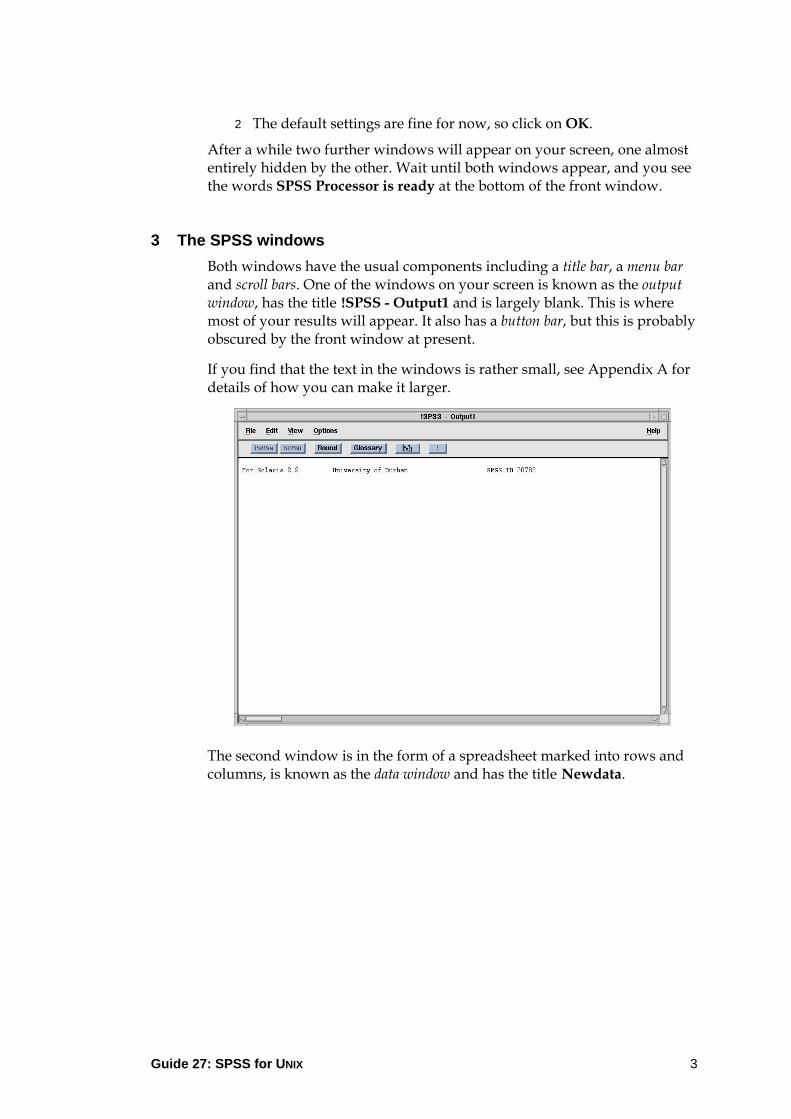
2 The default settings are fine for now, so click on OK.
After a while two further windows will appear on your screen, one almost entirely hidden by the other. Wait until both windows appear, and you see the words SPSS Processor is ready at the bottom of the front window.
3 The SPSS windows Both windows have the usual components including a title bar, a menu bar and scroll bars. One of the windows on your screen is known as the output window, has the title !SPSS - Output1 and is largely blank. This is where most of your results will appear. It also has a button bar, but this is probably obscured by the front window at present.
If you find that the text in the windows is rather small, see Appendix A for details of how you can make it larger.
The second window is in the form of a spreadsheet marked into rows and columns, is known as the data window and has the title Newdata.
Guide 27: SPSS for UNIX 3
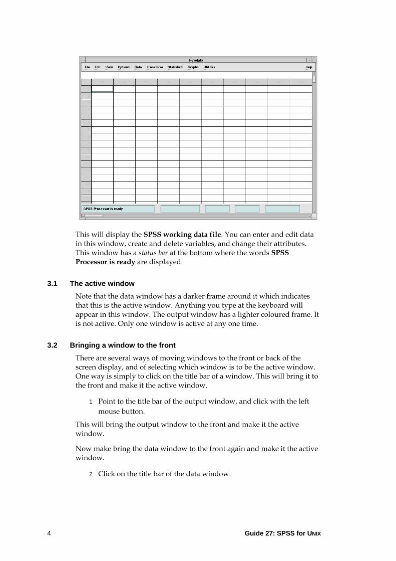
This will display the SPSS working data file. You can enter and edit data in this window, create and delete variables, and change their attributes. This window has a status bar at the bottom where the words SPSS Processor is ready are displayed.
3.1 The active window Note that the data window has a darker frame around it which indicates that this is the active window. Anything you type at the keyboard will appear in this window. The output window has a lighter coloured frame. It is not active. Only one window is active at any one time.
3.2 Bringing a window to the front There are several ways of moving windows to the front or back of the screen display, and of selecting which window is to be the active window. One way is simply to click on the title bar of a window. This will bring it to the front and make it the active window.
1 Point to the title bar of the output window, and click with the left mouse button.
This will bring the output window to the front and make it the active window.
Now make bring the data window to the front again and make it the active window.
2 Click on the title bar of the data window.
Guide 27: SPSS for UNIX 4
Guide 27: SPSS for UNIX 5
3.3 Moving windows You can reposition the windows on your screen as follows:
(Use this technique to move the output window to the bottom right corner of your screen.)
1 Point to the title bar of a window.
2 Press down on the left mouse button and drag the outline of the window to a new position.
3 Release the mouse button.
4 Using the same technique, move the data window to the top left corner of your screen.
3.4 Using the menu bar Beneath the title bar in each window is a menu bar, from which you can select commands from the File menu, the Edit menu and so on. Each window also has a Help menu. Notice that the list of menus is different for different windows.
1 Make the Data window the active window.
2 Open the File menu - point to File and click with the left mouse button.
A list of File commands will be displayed. Some of the commands are grey, and some are black. The grey ones are not available to you at this time. Notice the Exit command at the bottom of the list. When you have finished with SPSS you will need to select Exit from this menu.
3 Click outside the list of menu commands to close the list as you do not need any of these commands for the moment.
If you inadvertently find yourself in a menu or a dialog box that you don't want, then click on the Cancel button (if there is one) or press the Esc key. You may have to do this several times in order to close down all menus.
3.5 Viewing different parts of the content of a window. Frequently a window will contain more information than can be viewed at any one time, and you may need to bring other parts of it into view.
1 Bring the data window to the front if necessary.
To bring into view the content that is off the bottom of the screen:
2 Click on the small downwards pointing triangle near the bottom right hand corner of the window.
3 Repeat this last action several times.

Guide 27: SPSS for UNIX 6
The top rows of the spreadsheet will disappear, and new rows will appear at the bottom of the window. (You will need to look very closely at the left end of each row to see the very faint grey row numbers changing!)
4 Now scroll back up by pointing and clicking on the upward pointing triangle near the top right hand corner of the window.
Notice how the small rectangle between the triangles moves up and down as you scroll the window up and down. This is called the slider. You can scroll the window up and down by dragging the slider up and down.
5 Use the slider to scroll the window down and up again.
There is a horizontal scroll bar at the bottom of the screen with scroll buttons and a slider.
6 Use this to scroll the window to left and right.
7 Now return to the home position by dragging each slider to its starting position (top/left).
4 The working data file The data window displays the data in the SPSS working data file in the form of a spreadsheet. At present this is blank as you have not yet entered any data.
Consider the following hypothetical data (which you will shortly enter into the SPSS working data file), which consists of scores for the variables age, sex and income for a sample of 10 people.
Case ID Age Sex Income 1 38 F 0 2 27 M 32000 3 22 X 15000 4 31 M 40000 5 99 F 17000 6 40 F 5000 7 99 M 21050 8 28 F 0 9 39 M 46000 10 20 M 19000
When you enter the data into the SPSS working data file, the data will appear much as it does in the table shown here. There will be a column for each variable, each variable will be given a name, and there will be a row for each of the 10 cases in the sample. Each case in the sample has been assigned a unique case ID which appears in the first column.

You will have to choose a name for each variable. Each variable name may be up to 8 characters long, may consist of letters and numbers, must start with a letter, (and may include a dot, or any of the characters @ # _ $). It may not include spaces. Variable names are not case sensitive - age, Age and AGE would all be regarded as the same variable. There are some reserved words which you cannot use for variable names:
all and by eq ge gt le lt ne not or to with
4.1 Entering data into the SPSS working data file
1 Make the data window the active window.
2 Use the scroll bars to ensure that you have the first column and the first row at the top left of the window.
4.1.1 Enter data for the Case ID variable
1 Click on any cell in the first column of the spreadsheet.
2 Click on Data in the menu bar, then select Define Variable.
The Define Variable dialog box opens:
3 In the Define Variable dialog box double click in the Variable Name box.
4 Type caseid
then click on OK.
Guide 27: SPSS for UNIX 7

Guide 27: SPSS for UNIX 8
Notice that the variable name you have just entered appears above the first column of the spreadsheet.
5 Click in the first cell.
6 Type the first score 1
then press Enter.
Notice that the score 1.00 now appears in the first cell, and the highlight moves down to the next cell.
7 Now type the second score 2
then press Enter.
8 Repeat this until you have entered all 10 scores.
Note that it does not matter if you make mistakes as you are entering the data. You will have the opportunity to correct any errors in the data, or change a variable name, later on.
4.1.2 Enter the data for the Age variable
1 Using a similar procedure, enter the data for the age variable into the second column of the spreadsheet.
Use age as the variable name.
4.1.3 Enter data for the Sex variable
1 Click on any cell in the third column of the spreadsheet.
2 Click on Data in the menu bar, then select Define Variable.
3 In the Define Variable dialog box type sex
as the variable name.
Now you have to declare that the scores for this variable are characters not numbers.
4 Click on the Type button.
The following dialog box opens:
5 In the Define Variable Type dialog box, click on String.
6 Click on Continue.
7 In the Define Variable window, click on OK.
Notice that the variable name you have just entered appears above the third column of the spreadsheet.
8 Click in the first cell of the third column.
9 Type the first score F
10 Press Enter.
It is important that you type this as F rather than f.
Notice that the score F now appears in the first cell.
If it won't accept a score of F (it beeps when you type F), then you probably did not declare this variable to be a string variable. Repeat the data definition procedure for the sex variable, taking care that you do not omit anything.
11 Now type the second score M
and press Enter.
12 Repeat this until you have entered all 10 scores.
4.1.4 Enter the data for the Income variable
1 Using a similar procedure to that used for the caseid variable, enter the data for the income variable into the fourth column of the spreadsheet.
Guide 27: SPSS for UNIX 9

Guide 27: SPSS for UNIX 10
Use income as the variable name.
4.2 Check and edit the data in the spreadsheet
1 Check all the scores you have entered against the original table of data.
If you find an error:
1 Click in the cell that is wrong.
2 Type the correct value and press Enter.
If you can find no errors:
1 Click in any of the data cells.
2 Type in a new score and press Enter.
3 Repeat these steps to restore the correct value.
Note that variable names may also be edited using the Define Variable dialog box.
Notice how easy it is to correct the data in the spreadsheet. Take care though - it is equally easy to corrupt a data file!
4.3 Printing the data It is often easier to check the data that you have entered into SPSS with a printed listing rather than viewing it on the screen.
You can choose the printer and the quality of printing that you want.
There are two kinds of output - ASCII and PostScript. If you choose ASCII, you get just the data values printed, and you have no control over the character size. It will look something like this:
caseid age sex income 01 1.00 38.00 F .00 02 2.00 27.00 M 32000.00 03 3.00 22.00 X 15000.00 04 4.00 31.00 M 40000.00 05 5.00 99.00 F 17000.00 06 6.00 40.00 F 5000.00 07 7.00 99.00 M 21050.00 08 8.00 28.00 F .00 09 9.00 39.00 M 46000.00 10 10.00 20.00 M 19000.00
Guide 27: SPSS for UNIX 11
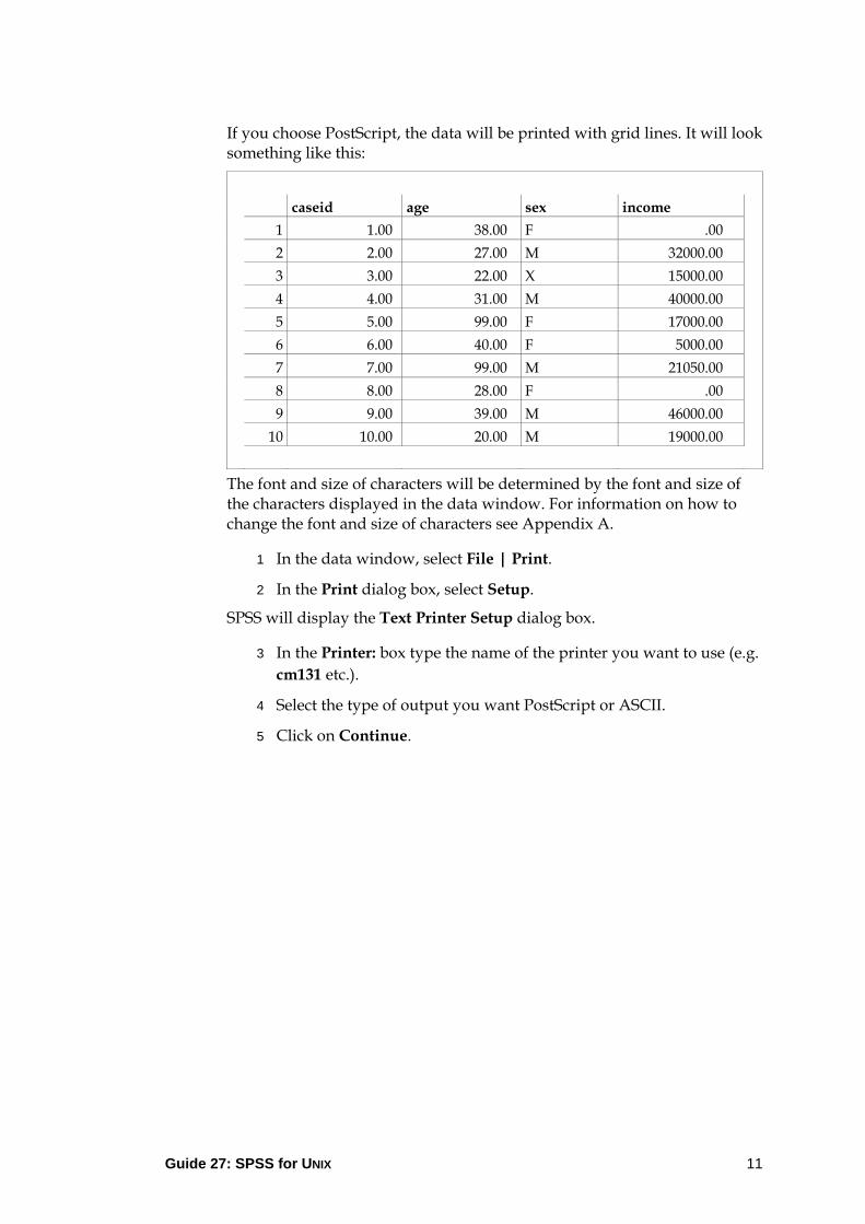
If you choose PostScript, the data will be printed with grid lines. It will look something like this:
caseid age sex income 1 1.00 38.00 F .00 2 2.00 27.00 M 32000.00 3 3.00 22.00 X 15000.00 4 4.00 31.00 M 40000.00 5 5.00 99.00 F 17000.00 6 6.00 40.00 F 5000.00 7 7.00 99.00 M 21050.00 8 8.00 28.00 F .00 9 9.00 39.00 M 46000.00 10 10.00 20.00 M 19000.00
The font and size of characters will be determined by the font and size of the characters displayed in the data window. For information on how to change the font and size of characters see Appendix A.
1 In the data window, select File | Print.
2 In the Print dialog box, select Setup.
SPSS will display the Text Printer Setup dialog box.
3 In the Printer: box type the name of the printer you want to use (e.g. cm131 etc.).
4 Select the type of output you want PostScript or ASCII.
5 Click on Continue.

6 In the Print dialog box click on OK.
4.4 Saving the SPSS working data file Now that you have entered all the data, you need to save them in a file. The Save and Save As commands save all the data in the SPSS working file (as displayed in data window), together with all the data definition information (i.e. the variable names), as an SPSS data file.
1 In the data window, select File | Save As.
The Save As Data File dialog box will open.
Guide 27: SPSS for UNIX 12

2 Click in the Selection box at the bottom of the Save As Data File dialog box, to the right of the path details.
3 Type sample1.sav
as the name for your file.
4 Click on OK.
The SPSS working data file will be saved as an SPSS data file in your stats directory, which you will be able to retrieve later.
Every time you save an SPSS working data file as an SPSS data file you should choose a name for your file that ends with .sav - this way you will be able to distinguish it from other sorts of files.
Notice that the title bar of the data window now displays the name you have given for your SPSS data file.
Note that an SPSS data file is in a format that only SPSS can read. You should not attempt to list, edit or print it.
Guide 27: SPSS for UNIX 13
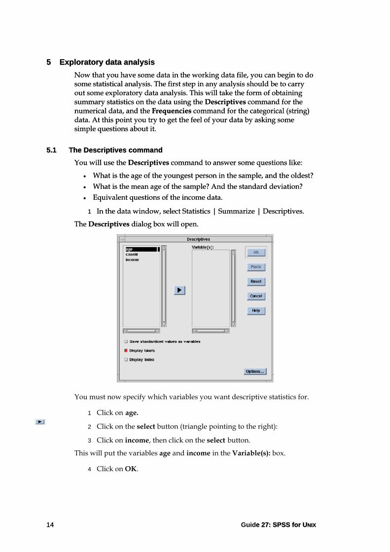
5 Exploratory data analysis 5 Exploratory data analysis Now that you have some data in the working data file, you can begin to do some statistical analysis. The first step in any analysis should be to carry out some exploratory data analysis. This will take the form of obtaining summary statistics on the data using the Descriptives command for the numerical data, and the Frequencies command for the categorical (string) data. At this point you try to get the feel of your data by asking some simple questions about it.
Now that you have some data in the working data file, you can begin to do some statistical analysis. The first step in any analysis should be to carry out some exploratory data analysis. This will take the form of obtaining summary statistics on the data using the Descriptives command for the numerical data, and the Frequencies command for the categorical (string) data. At this point you try to get the feel of your data by asking some simple questions about it.
5.1 The Descriptives command 5.1 The Descriptives command You will use the Descriptives command to answer some questions like: You will use the Descriptives command to answer some questions like:
• What is the age of the youngest person in the sample, and the oldest? • What is the age of the youngest person in the sample, and the oldest? • What is the mean age of the sample? And the standard deviation? • What is the mean age of the sample? And the standard deviation? • Equivalent questions of the income data. • Equivalent questions of the income data.
1 In the data window, select Statistics | Summarize | Descriptives. 1 In the data window, select Statistics | Summarize | Descriptives.
The Descriptives dialog box will open. The Descriptives dialog box will open.
You must now specify which variables you want descriptive statistics for.
1 Click on age.
2 Click on the select button (triangle pointing to the right):
3 Click on income, then click on the select button.
This will put the variables age and income in the Variable(s): box.
4 Click on OK.
Guide 27:e 27: SPSS for UNIX SPSS for UNIX 1414

Guide 27: SPSS for UNIX 15
The following descriptive statistics on the variables selected will appear in the Output window. You may have to bring it to the front in order to see the results. Look at the results and use them to answer your questions about the data.
Number of valid observations (listwise) = 10.00 Valid Variable Mean Std Dev Minimum Maximum N Label AGE 44.30 29.63 20.00 99.00 10 INCOME 19505.00 15911.74 .00 46000.00 10
5.2 Missing Values Notice that the maximum age is given as 99, and if you look at the data you will see that this value has been included in the calculation of the mean and other statistics. However the value 99 was not intended to be a valid score, but was intended to indicate that for some reason this score was missing - perhaps because the person refused to answer the question. So now you must tell SPSS that a score of 99 for the variable age is to be treated as a missing value. You will do this using the Missing Values command.
An alternative way to indicate that a score is missing is to leave the corresponding cell blank. SPSS will automatically treat blanks as missing.
However there may be times when a score might be missing for one of a number of different reasons (for example, a question was not relevant, or the person refused to answer) and you might want to record the reason. In this case you would have to code each reason with a different value.
For example:
99=refused to answer
98=question not relevant
Then you would use the Missing Values command to tell SPSS that both these values for the particular variable are to be regarded as missing. Note that the missing value must be appropriate for the variable: you must use a numerical missing value for a numerical variable, a character missing value for a character variable.
5.3 The Missing Values command Now tell SPSS that the value 99 for age is to be treated as missing.
1 In the data window, click on any cell in the column for the age variable.
2 Select Data | Define Variable.
3 In the Define Variable dialog box, click on the Missing Values button.
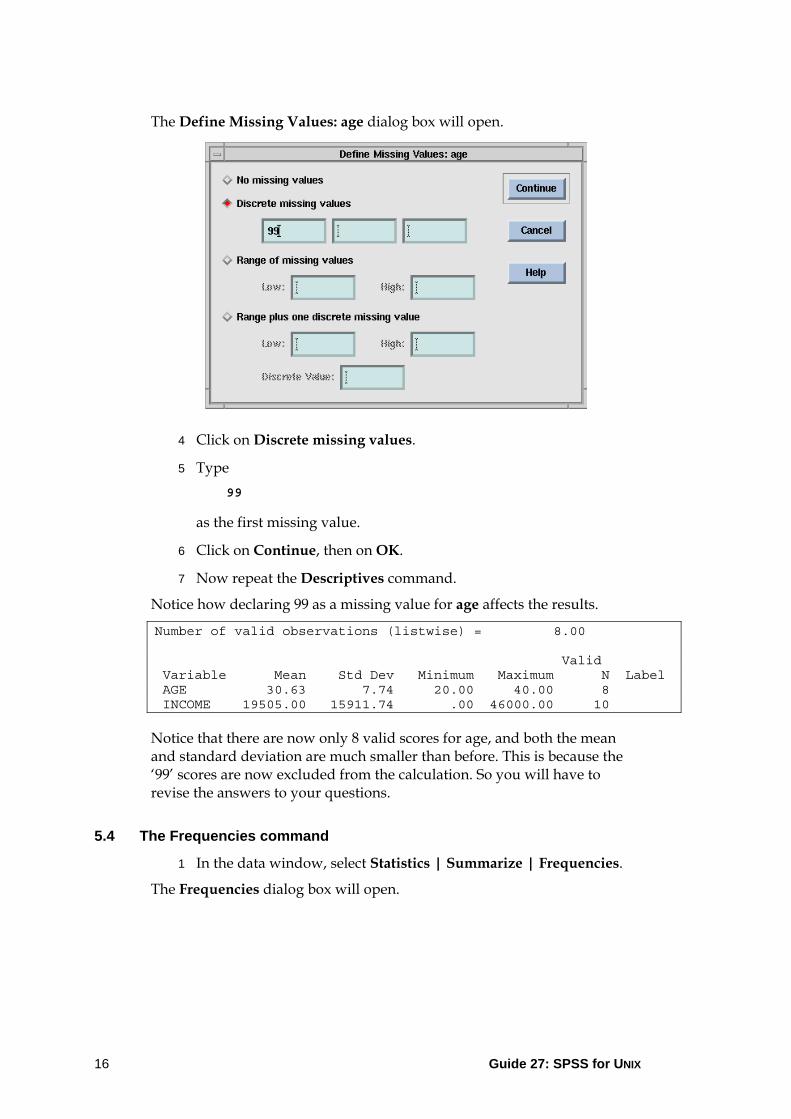
The Define Missing Values: age dialog box will open.
4 Click on Discrete missing values.
5 Type 99
as the first missing value.
6 Click on Continue, then on OK.
7 Now repeat the Descriptives command.
Notice how declaring 99 as a missing value for age affects the results.
Number of valid observations (listwise) = 8.00 Valid Variable Mean Std Dev Minimum Maximum N Label AGE 30.63 7.74 20.00 40.00 8 INCOME 19505.00 15911.74 .00 46000.00 10
Notice that there are now only 8 valid scores for age, and both the mean and standard deviation are much smaller than before. This is because the ‘99’ scores are now excluded from the calculation. So you will have to revise the answers to your questions.
5.4 The Frequencies command
1 In the data window, select Statistics | Summarize | Frequencies.
The Frequencies dialog box will open.
Guide 27: SPSS for UNIX 16

You must now specify which variables you want frequencies statistics for.
2 Click on sex.
3 Click on the select button.
4 Click on OK.
The following frequencies statistics on the variable selected will appear in the output window. You may have to bring it to the front in order to see the results.
SEX Valid Cum Value Label Value Frequency Percent Percent Percent F 4 40.0 40.0 40.0 M 5 50.0 50.0 90.0 X 1 10.0 10.0 100.0 ------- ------- ------- Total 10 100.0 100.0 Valid cases 10 Missing cases 0
Notice that the value X is treated exactly the same as F and M.
1 Use the Missing Values command to declare X as a missing value for sex.
Notice how this affects the output.
Guide 27: SPSS for UNIX 17

Guide 27: SPSS for UNIX 18
SEX Valid Cum Value Label Value Frequency Percent Percent Percent F 4 40.0 44.4 44.4 M 5 50.0 55.6 100.0 X 1 10.0 Missing ------- ------- ------- Total 10 100.0 100.0 Valid cases 9 Missing cases 1
Note that if the data consisted of a mix of upper case and lower case (F f M m X x), then these would be seen as 6 different values and would be counted separately.
You should now save the changes to the SPSS working data file.
1 In the data window, select File | Save.
This will save the missing values declarations, plus any other changes you may have made since the last time you saved the file. Notice that this time you do not have to provide a filename. SPSS uses the filename that appears in the title bar at the top of the data window. The previous contents of this file will be overwritten.
6 The output window Often there will be some results in your output window that you want either to print, or to save to a file for inclusion in a report of your findings. Usually there will also be some material in the output window that you want to discard, or you may wish to add something - perhaps some comments about your interpretation of the results, or about any unusual scores.
6.1 Editing the output window SPSS provides simple editing of the text in the output window.
You can point and click with the mouse to position the text insertion point, then insert new text, or delete text character by character using the backspace key.
You can click-and-drag the mouse over any amount of text to select it. Then you can delete, copy or move the selected text in the standard way using the Cut, Copy, Paste or Clear commands from the Edit menu. Take care with the Edit | Clear command - in the output window cleared text cannot be replaced!
Guide 27: SPSS for UNIX 19
1 Experiment with some editing operations - for example delete some text, and add some new text.
There may be times when you want to delete everything in the output window. Use Edit | Select All to highlight all the text, then choose Edit | Clear- but do not do this at present!
6.2 Saving the output window You can save the whole content of the output window, or you can select some text and save just what you have selected.
1 If required, select the area in the output window that you want to save.
2 In the output window, select File | Save As.
3 Type sample1.lst in the Selection box, then click on OK.
When saving your output window you should always choose a name that ends with .lst to distinguish it from your other files.
If you highlighted some text before you clicked on File | Save As a box will open up asking you Save the selected area only?
1 Answer Yes to save just the selected text, answer No to save everything in the output window, or answer Cancel to save nothing.
6.3 Printing the output window You can print the whole content of the output window, or you can select part of it and print just what you have selected.
You can also choose the printer and the quality of printing that you want, in the same way as for the data window. As with the data window there are two kinds of output - ASCII and PostScript. If you choose PostScript, the font and size of characters will be determined by the font and size of the characters displayed in the output window. For information on how to change the font and size of characters see Appendix A.
1 If required, select the area in the output window that you want to print.
2 In the output window, select File | Print.
3 In the Print dialog box, select Setup.
SPSS will display the Text Printer Setup dialog box.

4 Type the name of the printer you want to use in the Printer: box.
5 Select the type of output you want PostScript or ASCII.
6 Click on Continue.
7 In the Print dialog box, choose Selection if you selected some text to print, otherwise choose All, then click on OK.
7 Using the online help The UNIX version of SPSS includes a hypertext based Help system. It includes information on how to run SPSS, what commands to use and how to interpret your results. The best way to learn about the Help system is to use it.
There are several ways to access the Help system:
• Select Help from the menu bar in any SPSS window. • Click on the Help button in an SPSS dialog box for information about
the dialog box and what it can do. • Click on the Glossary button in the output window for definitions of
statistical terms.
The Help system also provides information on how to use the Help system!
Experiment with the Help system to answer the following questions:
Q1 How can you enter data by case (i.e. by rows) instead of by variable (i.e. by column)?
Guide 27: SPSS for UNIX 20

Q2 How can you edit the text in the output window (i.e. insert new text, delete text, move or copy text)?
Q3 What does the Labels button in the Define Variable dialog box allow you to do?
Q4 What sorts of facilities are available to you for creating new variables?
When you are finished with the Help system, close it down by selecting File | Close from the Help window.
8 Ending the SPSS session
8.1 Closing down SPSS
1 Select File | Exit.
This can be done from either window.
If you have made any changes to the working data file since you last saved it you will be asked if you want to save the changes.
2 Click on Yes if there are changes you want to save, otherwise click on No.
If you have made any changes to the output window since you last saved it, you will be asked if you want to save the changes.
3 Click on Yes if there are changes you want to save, otherwise click on No.
The SPSS processor will stop and you will be returned to the UNIX prompt in the terminal window.
1 Type ls
Guide 27: SPSS for UNIX 21

to display a list of the names of the files in your current directory. You should see the filename sample1.sav (the SPSS data file in which you saved your data), and sample1.lst (the text that you saved from the output window).
8.2 Retrieving a saved data file
1 Start up SPSS again and retrieve the data file that you have been working on.
Wait till the both SPSS windows appear, and you see the message
SPSS Processor is ready
at the bottom of the data window.
2 Move the SPSS windows to where you want them on the screen.
3 In the data window, select File | Open | Data.
The Open Data File dialog box will open:
4 In the Open Data File dialog box, click on the name of your file (sample1.sav), then click on OK.
Guide 27: SPSS for UNIX 22

Guide 27: SPSS for UNIX 23
This will load the file you saved earlier and you should see the data displayed in the spreadsheet.
5 Repeat some of the exploratory data analysis that you did earlier.
Provided you saved the data after declaring the missing values you should find that the missing values are treated correctly - they should be excluded from the summary statistics produced by the Descriptives command, and counted as missing by the Frequencies command.
9 Managing your data It is not always convenient to key your data into the SPSS spreadsheet. It may be that your data have been generated by another program and are available as a spreadsheet or text file.
For this session you will read some data from a sample text file that has been prepared for you. You will need to take a copy of this file and put it in your stats directory along with the other files you will be using for the SPSS course.
1 Login to a UNIX workstation in the usual way.
2 Open a terminal window.
3 Make the stats directory the current directory by typing cd stats
4 Copy the file /usr/local/courses/spss/survey1.dat to the current (stats) directory by typing
cp /usr/local/courses/spss/survey1.dat survey1.dat
This file contains the hypothetical data that you will be working on for this session. It will be helpful to take a look at what is in it.
5 Type head survey1.dat
to display the first 10 lines of the file.
There are in fact 50 lines of data in the file.
1 F 38 M 2 0 648 657 2 M 27 M 3 32000 559 580 3 X 22 S 2 15000 646 998 4 M 31 M 4 40000 668 646 5 F 99 S 0 17000 645 998 6 F 40 M 3 5000 724 623 7 M 99 M 3 21050 651 580 8 F 28 M 1 0 591 746 9 M 39 S 0 46000 728 998 10 M 20 S 0 19000 681 998

Guide 27: SPSS for UNIX 24
The data consist of 8 scores for each of 50 people. The following table gives, for each score, a name, the column range, the type (whether numeric or alphanumeric), the number of decimal places (if numeric), a description of the score, and any missing value scores.
Name Columns Type Places Description Missing values
Person 1-3 N 0 Identifying code Sex 5 A Sex X Age 8-9 N 0 Age 99 Marstat 11 A Marital status Nkids 14 N 0 Number of children 9 Income 17-21 N 0 Annual income 99999 Height 23-25 N 1 Height 999 Sheight 27-29 N 1 Height of spouse 998, 999
Note that the scores for Height and Sheight are measured in inches, but are entered in the data file without the decimal point - the first score appears in the data file as 648 but it is to be taken as 64.8. When you read the data into SPSS you will need to tell SPSS to insert the decimal point before the last figure.
Note also that there are two missing scores for Sheight - 998 is used if the person is not married and so has no spouse, 999 is used if the person is married but refused (or was unable) to answer the question.
You are now going to get SPSS to read these data.
1 Start SPSS
Wait till both the SPSS windows appear and you see the message SPSS Processor is ready at the bottom of the data window.
2 Move the windows to where you want them on the screen.
9.1 The Read ASCII Data command
1 In the data window, select File | Read ASCII Data.
This will open up the Read ASCII Data File dialog box.
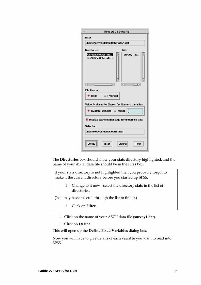
The Directories box should show your stats directory highlighted, and the name of your ASCII data file should be in the Files box.
If your stats directory is not highlighted then you probably forgot to make it the current directory before you started up SPSS.
1 Change to it now - select the directory stats in the list of directories.
(You may have to scroll through the list to find it.)
2 Click on Filter.
2 Click on the name of your ASCII data file (survey1.dat).
3 Click on Define.
This will open up the Define Fixed Variables dialog box.
Now you will have to give details of each variable you want to read into SPSS.
Guide 27: SPSS for UNIX 25
Guide 27: SPSS for UNIX 26
For the Person variable:
1 in the Name box, type person
2 Press the Tab key to move to the next box.
3 in the Record box, type 1
4 Press Tab again to move on the next box.
5 in the Start Column box, type 1
6 Press Tab again to move on the next box
7 in the End column box, type 3
8 in the Data Type box, make sure that Numeric as is is selected.
9 then click on Add.
Enter the following values for the Sex variable in the same way (press Tab to move to the next box):
1 In the Name box, type sex
2 In the Record box, type 1
3 In the Start Column box, type 5
4 In the Data Type box, select String (A).
5 Click on Add.
6 Enter the appropriate details for the rest of the variables.
Note that for height and sheight you will need the data type Numeric 1 decimal (1).

If you need to modify any details, then
1 Click on the variable in question in the list of Defined Variables.
2 Make the required changes to the details.
3 Click on Change.
When you have finished entering the details for all the variables, the Define Fixed Variables dialog box should look like this:
When all the details are correct,
7 click on OK.
After a few moments you will see the scores from the file survey1.dat appearing in the data window.
8 Look at the scores carefully to make sure that they have been read correctly.
If the scores have not been read correctly, repeat the Read ASCII Data command and correct the entries in the Define Fixed Variables dialog box.
9.2 Save the working data file When you are satisfied that the data have been read correctly:
1 Save the working data file as an SPSS data file using the File | Save As command.
The Directories box in the Save As Data File dialog box should show your stats directory highlighted, and the name of your SPSS data file from the previous session (sample1.sav) should be in the Files box.
Guide 27: SPSS for UNIX 27
Guide 27: SPSS for UNIX 28
2 Click in the Selection box and type survey1.sav
as the name for your new file.
3 Click on OK.
This will save the data together with the variable names that you have provided as an SPSS data file. Next time you want to work on these data, you will be able to use the File | Open | Data command instead of repeating the Read ASCII Data command.
9.3 Assign missing values Some of the variables have values that need to be declared as missing.
1 Declare as missing the appropriate values of all the variables that have missing values.
2 Run the Frequencies or Descriptives command (as appropriate) on the variables with missing values.
3 Look at the output to confirm that the missing values have been declared correctly.
If they are wrong, then you will need to repeat the Missing Values command with appropriate modifications.
This changes the working data file.
4 Save these changes to the SPSS data file using the File | Save command.
9.4 Data validation It is a very important part of any analysis that you validate the scores at an early stage.
If there are errors that need to be corrected, then the sooner you can identify them and correct them the less likely you are to come to false conclusions about your data. For instance there may be simple mistakes in the coding or entering of the data. Unusual scores may indicate a problem with the procedure used to collect the data, which might require a possible re-evaluation of the methods used. Alternatively there may be genuinely unusual scores that need special treatment. At the very least, the early identification of unusual values can help to reduce the amount of re-analysis that you will have to do.
1 Apply the Frequencies command to the variables that have discrete values.
2 Apply the Descriptives command to the other scores.

Guide 27: SPSS for UNIX 29
3 Look at the output.
It is very important to look at the output! Do the results indicate the presence of any unusual scores? Are you getting the results you expect? Of course you will need to know something about your data in order to know what results you should expect! So ask yourself some questions of the data. For example:
• Should you have roughly equal numbers of males and females? • Do you expect the males to be taller on average than the females? • What sort of range of incomes would you expect? • You should find that there are no spouse values for people who are
not married.
Finding answers to simple questions like these will help you to get the feel of your data. When working with your own data you would need to check any unusual scores against the original source of the data. You would correct them if they were wrong, or if not, consider why they were unusual and whether you need to modify your method of data collection or rethink your plans for the analysis of the data.
9.5 Applying labels to your data You can provide descriptive variable and value labels which can make your output much more readable/meaningful.
Variable labels give additional information about variables. Variable labels can be up to 120 characters long.
Value labels give additional information about values. Value labels can be up to 60 characters long.
1 Click on any cell in the marstat column of data.
2 Select Data | Define Variable.
3 In the Define Variable dialog box, click on Labels.
4 In the Define Labels dialog box, type Marital status
as the Variable Label.
5 In the Value Labels box, type S
as the Value.
Note that this must be capital S not lower case s.
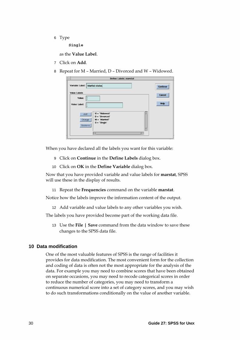
6 Type Single
as the Value Label.
7 Click on Add.
8 Repeat for M – Married, D – Divorced and W – Widowed.
When you have declared all the labels you want for this variable:
9 Click on Continue in the Define Labels dialog box.
10 Click on OK in the Define Variable dialog box.
Now that you have provided variable and value labels for marstat, SPSS will use these in the display of results.
11 Repeat the Frequencies command on the variable marstat.
Notice how the labels improve the information content of the output.
12 Add variable and value labels to any other variables you wish.
The labels you have provided become part of the working data file.
13 Use the File | Save command from the data window to save these changes to the SPSS data file.
10 Data modification One of the most valuable features of SPSS is the range of facilities it provides for data modification. The most convenient form for the collection and coding of data is often not the most appropriate for the analysis of the data. For example you may need to combine scores that have been obtained on separate occasions, you may need to recode categorical scores in order to reduce the number of categories, you may need to transform a continuous numerical score into a set of category scores, and you may wish to do such transformations conditionally on the value of another variable.
Guide 27: SPSS for UNIX 30

SPSS provides a number of tools for transforming data, from simple tasks, like adding two scores together, to complex tasks based on complex equations and conditional statements.
Each time you create a new variable, or modify an existing variable, you must look at the values generated to make sure that SPSS has done what you wanted. It does of course do what you tell it to do, but sometimes it is all too easy to get the instructions wrong!
When transforming data it is normally advisable to create a new variable (rather than overwriting an existing variable). If you make an error in your instructions then you can always try again if you have created a new variable, whereas if you modified an existing variable you may have destroyed the values you need to perform the calculation correctly.
10.1 The compute command Create two new variables for the height and the spouse's height in centimetres.
1 Select Transform | Compute.
2 In the Compute Variable dialog box enter a name for the new variable in the Target Variable box.
3 Click on Type & Label.
4 Provide an appropriate variable label for the new variable.
5 Click on Continue.
6 Build the appropriate expression in the Numeric Expression box.
You can do this by typing it in, or by clicking on the appropriate buttons on the calculator pad. (See Appendix B for a list of the operators you can use and their functions.)
For example:
1 Click on height.
2 Click on the select button.
3 Type in *2.54
Guide 27: SPSS for UNIX 31
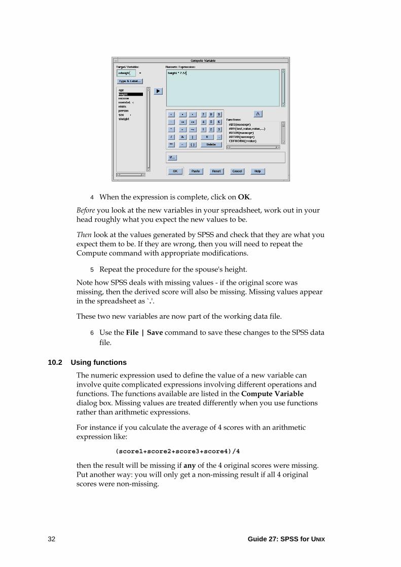
4 When the expression is complete, click on OK.
Before you look at the new variables in your spreadsheet, work out in your head roughly what you expect the new values to be.
Then look at the values generated by SPSS and check that they are what you expect them to be. If they are wrong, then you will need to repeat the Compute command with appropriate modifications.
5 Repeat the procedure for the spouse's height.
Note how SPSS deals with missing values - if the original score was missing, then the derived score will also be missing. Missing values appear in the spreadsheet as `.'.
These two new variables are now part of the working data file.
6 Use the File | Save command to save these changes to the SPSS data file.
10.2 Using functions The numeric expression used to define the value of a new variable can involve quite complicated expressions involving different operations and functions. The functions available are listed in the Compute Variable dialog box. Missing values are treated differently when you use functions rather than arithmetic expressions.
For instance if you calculate the average of 4 scores with an arithmetic expression like:
(score1+score2+score3+score4)/4
then the result will be missing if any of the 4 original scores were missing. Put another way: you will only get a non-missing result if all 4 original scores were non-missing.
Guide 27: SPSS for UNIX 32

Guide 27: SPSS for UNIX 33
If you use the sum function to do this:
sum(score1,score2,score3,score4)/4
or the mean function:
mean(score1,score2,score3,score4)
then the result will only be missing if all the 4 original scores were missing. In this case you could get a result based on only one score.
When using statistical functions like sum or mean, you can use a variation of the function which allows you to specify the minimum number of original scores that are required for the function to return a non-missing result, e.g.
mean.2(score1,score2,score3,score4)
will produce a result so long as at least two of the original scores are non-missing.
1 Create a new variable for the mean of the variables height and sheight which has a non-missing value provided at least one of the original scores is non-missing.
If you have difficulty with this, take a look at Appendix C, which contains solutions to selected exercises.
10.3 Deleting variables and cases from the working data file When managing your data you sometimes have to create new variables which are required only in order to complete subsequent transformations. It is not necessary to save them as part of the SPSS data file. Such variables should be deleted before the file is saved.
Sometimes you have cases in a file with invalid scores, or all missing scores, that you wish to remove. These cases can be deleted before the file is saved.
Delete the variable you have just created for mean height:
1 Click on the name of the variable at the top of the spreadsheet.
2 Select Edit | Clear.
The last case in the file has all missing values and needs to be deleted.
1 Click on the row number (51) at the left end of the row of the last case in the file. The whole row should be selected.
2 Select Edit | Clear.
The row should disappear. Note that each of these clear operations can be undone by selecting Edit | Undo Clear - provided this is done immediately after the Clear operation.

Guide 27: SPSS for UNIX 34
10.4 Conditional compute commands SPSS allows you to compute new variables conditionally on the values of other variables. To illustrate this create a new variable called status which will have values as follows:
1 married with children 2 married with no children 3 not married with children 4 not married with no children
You will need to run the Compute command four times to do this - once for each condition.
1 Select Transform | Compute.
2 In the Compute Variable dialog box type status
in the Target Variable box.
3 Click on Type & Label and provide an appropriate variable label for the new variable (e.g. Family Status).
4 Enter 1 for the Numeric Expression.
5 Click on If....
6 In the Compute Variable: If Cases dialog box, click on Include if case satisfies condition.
7 Enter marstat = 'M' & nkids >0
as the condition.
8 Click on Continue.
(See Appendix B for a list of the operators you can use and their functions.)

9 In the Compute Variable dialog box click on OK.
Repeat the above steps with appropriate modifications for the other values of status. In this case you will put status as the name of the new variable each time. For the second and subsequent transformations SPSS will ask you if it is OK to change an existing variable. At this point:
10 Click on OK.
Note that you must put M for marstat (m won't do), and you must enclose it in quotes. Use ~= for not equals.
11 Look at the values of the new variable in the spreadsheet and check that they are what you want them to be. If they are wrong, then you will need to repeat the Compute command with appropriate modifications.
12 Add appropriate value labels to the status variable.
13 Use the File | Save command to save these changes to the SPSS data file.
10.5 The recode command The recode command is useful if you need to transform a continuous numerical score into a set of category scores, or if you need to recode categorical scores in order to reduce the number of categories.
As with the compute command you can create new variables or modify existing variables. Again it is generally advisable to create new variables rather than modify existing ones.
Guide 27: SPSS for UNIX 35

For example you may wish to create a new categorical variable for income based on the following income bands:
income income category 0 0 1-5000 1 5001-10000 2 10001-20000 3 20001-30000 4 >30001 5
1 Select Transform | Recode | Into Different Variables
2 In the Recode into Different Variables dialog box select the variable name income.
3 Click on the select button.
4 In the Output Variable box, type an appropriate name and label for the new variable.
5 Click on Change.
6 Click on the Old and New Values... button.
In the Recode into Different Variables: Old and New Values dialog box fill in the details of the recoding required (as given in the above table):
1 In the Old Value box, click in the Value: box and type 0
2 In the New Value box, click in the Value: box and type 0
3 Click on Add.
Guide 27: SPSS for UNIX 36

4 In the Old Value box, click in the small button beside the first Range: and type
1
5 Click in the box after the word through and type 5000
6 In the New Value box, click in the Value: box and type 1
7 Click on Add.
8 Use steps 4 to 7 to recode income categories 2, 3 and 4 as shown in the table.
9 For income category 5, click in the button beside the third Range: (labelled through highest) and type
30001
10 In the New Value box, click in the Value: box and type 5
11 Click on Add.
To recode missing values for income:
1 In the Old Value box, click in the button beside System- or user-missing.
2 In the New Value box, click in System-missing.
3 Click on Add.
When you have entered all details required:
1 Click on Continue.
2 In the Recode into Different Variables dialog box click on OK.
Guide 27: SPSS for UNIX 37

Guide 27: SPSS for UNIX 38
Look at the values of the new variable in the spreadsheet and check that they are what you want them to be. If they are wrong, then you will need to repeat the Recode command with appropriate modifications.
1 Add appropriate value labels to the new variable.
2 Use the File | Save command to save these changes to the SPSS data file.
10.6 Conditional recode commands The recode command can be applied to selected cases in the same way as for the compute command.
1 Using conditional recode commands create a new variable called tall which has the value 1 for men 6 feet (72I) or taller and for women 5 feet 8 inches (68I) or taller, and has the value 0 for men less than 6 feet and women less than 5 feet 8 inches.
Make sure that you deal with any missing values appropriately.
Check the outcome by looking at the values of the new variable in the spreadsheet.
2 Run the Descriptives command on the variable height.
3 Run the Frequencies command on the new variable tall.
Check that you are getting the results you expect. Do the number of missing values match?
This categorisation of the values of the variable height could also have been done with conditional compute commands.
4 Create a new variable, tall2, using the conditional compute commands, which has the same values as given in step 1 above.
Look at the scores for the two variables tall and tall2. Do you get the same results? How can you check this?
10.7 The List command When checking the results of your transformations it may be difficult if you cannot see all the relevant variables without scrolling the spreadsheet. The List command can help in this situation. Use this to check the values you have just obtained for the tall and tall2 variable.
1 Select Statistics | Summarize | List Cases.
2 In the List Cases dialog box select each of the variables sex, height, tall and tall2, then click on OK.
Look at the output window to see a listing of just these four variables.

Guide 27: SPSS for UNIX 39
11 Using Syntax commands The process of running SPSS by selecting commands by clicking with the mouse on on-screen menus and selecting options from dialog boxes is fine when you are exploring your data or experimenting with SPSS. However there soon comes a time when you want to repeat a sequence of commands, perhaps with a new or enlarged data file, and then you may prefer to call up a prepared sequence of syntax commands which can be run with a single mouse click.
There are other occasions when the use of syntax commands can be preferable to selecting commands from the menus, specially when you may need to apply the same operations to many variables.
SPSS assists you in preparing such syntax commands in a number of ways.
• SPSS keeps a log of all the commands you run, in the form of syntax commands. These are stored in the file spss.jnl which is in your home directory.
• You can build up a file of syntax commands as you run SPSS from the on-screen menus, by pasting the commands you want into a syntax window.
• The online help provides details of all the syntax commands which can be useful if you want to enter new syntax commands, or modify existing ones.
You will learn how to make use of all of these during this session.
1 Login to a UNIX workstation in the usual way.
2 Open a terminal window.
Take a look at what is in the file spss.jnl which is in your home directory. Use an editor to look at the file, or display it by typing
more spss.jnl
This should be a list of the syntax command equivalents of all the SPSS commands you have used! You should see commands such as:
DATA LIST SAVE OUTFILE MISSING VALUES VARIABLE LABELS VALUE LABELS DESCRIPTIVES FREQUENCIES COMPUTE RECODE
For this session you will be running syntax commands from a sample file that has been prepared for you. This file is similar to your own spss.jnl file. You will need to take a copy of this and put it in your stats directory along with all the other files you will be using for the SPSS course.
For this session you will also read some data from another sample ASCII data file that has been prepared for you. This file survey2.dat is similar to

survey1.dat - it has the same variables but many more cases. You will need to take a copy of this file also and put it in your stats directory.
1 Make the stats directory the current directory by typing cd stats
2 Copy the file /usr/local/courses/spss/spss.jnl to the current (stats) directory and change its name to survey1.sps, by typing:
cp /usr/local/courses/spss/spss.jnl survey1.sps
3 Copy the file /usr/local/courses/spss/survey2.dat to the current (stats) directory, type:
cp /usr/local/courses/spss/survey2.dat survey2.dat
You are now going to get SPSS to select commands from the syntax file survey1.sps.
1 Start SPSS.
Wait till both the SPSS windows appear and you see the message SPSS Processor is ready at the bottom of the data window.
11.1 The Open Syntax command
1 In the data window, select File | Open | SPSS Syntax.
This will open up the Open SPSS Syntax dialog box.
The Directories box should show your stats directory highlighted, and the name of your SPSS syntax file (survey1.sps) should be in the Files box.
Guide 27: SPSS for UNIX 40

If your stats directory is not highlighted, then change to it now: ted, then change to it now:
1 Select the directory stats in the list of directories. 1 Select the directory stats in the list of directories.
2 Click on Filter. 2 Click on Filter.
2 Click on the name of the SPSS syntax file (survey1.sps). 2 Click on the name of the SPSS syntax file (survey1.sps).
3 Click on OK. 3 Click on OK.
This will open up a new window - a syntax window - in which you will see all the commands that were in the file survey1.sps. It has a title bar displaying the name of the file (complete with its full path), a menu bar and a tool bar.
This will open up a new window - a syntax window - in which you will see all the commands that were in the file survey1.sps. It has a title bar displaying the name of the file (complete with its full path), a menu bar and a tool bar.
11.2 SPSS Syntax command conventions Take a look at the commands in the syntax window. They obey the following rules:
• Each command starts with a command name at the beginning of a line.
• There are at most 80 characters on a line. • For commands that have continuation lines each continuation line is
indented. (It starts with at least one space).
• Some commands have subcommands which are separated from one another by forward slashes `/'.
• Each command is terminated by a period `.' the command terminator.
Guide 27: SPSS for UNIX 41
Guide 27: SPSS for UNIX 42
• Note also that commands and variable names can be typed in upper or lower case.
• File names are enclosed in quotes. • Blank lines can be used to separate commands and improve
readability.
You will now learn how to select and run commands from the syntax window.
11.3 Running syntax commands You can select individual commands to run, and you can run them in any order. You can also select a group of contiguous commands to run, or you can select all the commands in the window and run them. You will start with running single commands.
The first command in the file is the DATA LIST command. This is the equivalent of the File | Read ASCII Data command that you did earlier in these notes. It specifies the name of the file to be read, it lists the names of each of the variables and where in the file the scores for each variable are to be found. It also indicates where the decimal point is to go (for numeric variables), and which variables are string variables.
You are going to run this command from the syntax window, but before you do this you need to change the reference to the data file from survey1.dat to survey2.dat.
In the DATA LIST command change survey1.dat into survey2.dat:
1 Place the text insertion point after the 1 in survey1.dat.
2 Press the backspace key.
3 Type 2
Run the DATA LIST command:
1 Make sure the text insertion point is still somewhere within the DATA LIST command.
2 Click on the Run button on the toolbar.
After a little while you should see the variable names appearing in the data window, but no data! To get the data you have to run the EXECUTE command.
1 Select the EXECUTE command (point somewhere within it and click).
2 Click on Run.
Guide 27: SPSS for UNIX 43
After a little while you should see the data from the file survey2.dat appearing in the data window.
The next command in the file is the SAVE OUTFILE command. This is the equivalent of the File | Save As command that you used in Part B. It specifies the name of the file to be written to. You are going to run this command from the syntax window, but before you do this you need to change the reference to the data file from survey1.sav to survey2.sav.
3 In the SAVE OUTFILE command change survey1.sav into survey2.sav.
4 Run the SAVE OUTFILE command.
11.4 Making global changes in the syntax window You have already seen how to make simple changes to the commands in the syntax window. In this file there are several occurrences of survey1 that need to be changed to survey2. Instead of finding and changing each one separately, you can change them all at once.
1 Place the text insertion point at the beginning of the first command in the syntax window.
2 Select Edit | Replace Text.
3 In the Replace Text dialog box, type survey1
as the text to Search for, and survey2
as the Replace with text.
Notice that you can choose to search forward or backward from the text insertion point.
4 Click on Replace All.
SPSS will report to you how many times it makes the replacement.
5 Click on OK to close the message box.
6 Click on Cancel as you have no further global changes to make.
11.5 Saving the contents of the syntax window. Now that you have made a number of changes to the content of the syntax window you should save it to a syntax file. You will need to use the File | Save As command (rather than File | Save) so that you can give it a new name. An appropriate name for it would be survey2.sps.
1 In the syntax window, select File | Save As.

Guide 27: SPSS for UNIX 44
2 In the Save As !SPSS dialog box check that the directory you require is highlighted (if it isn't then select the one you want and click on Filter).
3 Type survey2.sps
in the selection box.
4 Click on OK.
Whenever you save a syntax window you should choose a name that ends with .sps to distinguish syntax files from your other files.
Note that this new name appears in the title bar of the syntax window.
11.6 Selecting and running several commands at once You can select several commands to run one after the other, rather than having to select each one individually. You need to run a few groups of commands now.
Run the MISSING VALUES commands now. To select these commands:
1 Drag the mouse over all the required commands until you have highlighted at least part of each command.
2 Click on Run.
Run the VARIABLE LABELS command and the VALUE LABELS command for marstat:
1 Select both of them.
2 Click on Run.
11.7 Mixing menu commands with syntax commands It is not necessary to continue to use syntax commands once you have started to use them. You may go back to using menu commands whenever you wish. For instance you could now use a menu command to save the working data file.
1 Make the data window the active window.
2 Use the File | Save command to save the working data file.
3 Make the syntax window active again.
4 Run the transformation commands to create the new variables status, incomcat and tall.
You will have to scroll down the syntax window to find these commands.

Guide 27: SPSS for UNIX 45
5 Look at the new scores in the data window and verify that they are correct.
6 Save the working data file using either one of the SAVE OUTFILE commands in the syntax window, or by clicking on the File | Save command from the data window.
11.8 Pasting menu commands into the syntax window It is possible to select commands from the on-screen menus in the usual way, and then paste them into a syntax window. In this way you can build up new commands in the syntax window without knowing the correct syntax to use, or even the correct command name.
You will use this to create and run a command for generating a two way frequency table to look at the relationship between income and height using the two categorical variables incomcat and tall.
1 In the data window, select Statistics | Summarize | Crosstabs.
2 In the Crosstabs dialog box, select incomcat as the row variable, and tall as the column variable.
3 Click on Paste.
Instead of running the command, SPSS puts the corresponding syntax command into the syntax window at the end.
4 In the syntax window, select the new CROSSTABS command and run it.
5 Look at the output.
On looking at the output you might decide that it would be helpful to add row and/or column percents to the output in order to interpret the results. To do this, you could explore the options in the Crosstabs dialog box, or you could use the online help to make the necessary changes to the CROSSTABS syntax command as described in the next section.
11.9 Getting help with syntax commands Sometimes you know the name of a command but are not sure of the exact syntax, or of what options are available. Or you may want to modify an existing command and need some help with it. There is a quick way to access the online Help system to find information about the syntax of a command in the syntax window.
11.10 Modifying an existing command
1 In the syntax window, select the CROSSTABS command.
2 Click on the Syntax button in the tool bar.
Guide 27: SPSS for UNIX 46
SPSS will display details of the CROSSTABS command. Anything in square brackets [] is optional, anything in upper case you type as it is, anything in lower case you have to replace with your own requirements. You choose between items enclosed within braces {}, and ... means more of the same (e.g. varlist ... is used to indicate a list of variable names separated by commas or spaces).
1 Rearrange the windows if necessary so that you can keep the Help visible whilst you edit the syntax window.
2 Using the Help information, modify the CROSSTABS command to request row and column percents as well as the counts for each cell.
3 Run the modified CROSSTABS command and look at the output.
When you are done with the Help, close the Help window:
1 Select File | Close in the Help window.
11.11 Creating a new command The variables incomcat and tall have no value labels assigned to them. You are now going to create and run a new syntax command to provide appropriate value labels. You can find out what to do by looking at other VALUE LABELS commands, or you could use the syntax help.
1 In the syntax window look at the commands for creating value labels.
2 Type VALUE LABELS
as a new command at the end of the syntax window.
3 With the text insertion point still within this command click on Syntax.
SPSS will display details of the VALUE LABELS command..
4 Using the help information complete the syntax command to provide appropriate value labels for incomcat and tall.
(Don't forget the command terminator.)
5 Run your new VALUE LABELS command.
6 Re-run the CROSSTABS command and see how the use of value labels improves the information content of your output.
7 When you are done with the Help, close the Help window.
8 Save the working data file.
9 Save the revised syntax window.

Guide 27: SPSS for UNIX 47
10 Save and/or print any of the output you wish.
11.12 Creating an SPSS program The commands in a syntax window can be used as the basis for an SPSS program. Such a program would consist of a set of commands that you would want to run sequentially. In future you would be able to run the whole program by selecting all the commands in the syntax window and clicking on Run.
The commands in your syntax window could now be modified to form a program that could be used in the initial stages of a project based on the survey data. You would need to keep those commands that read the data from the ASCII data file and provide all the data definition information (missing values, variable labels and value labels). You would also need to keep the commands to create the new variables that you would need for further analysis. You would also need the commands to perform the exploratory data analysis so that you could validate your data before proceeding with any further analysis. And finally you would need the command to save the data as an SPSS data file.
In addition you can add explanatory comments to an SPSS program. Comments can contain any text. They begin with the word comment (or an asterisk *), and should end with the usual command terminator. Examples of comment lines are:
COMMENT This is an example of an SPSS program .
Comment The file survey2.dat contains some hypothetical data .
*Now save the working data file as an SPSS data file .
1 Modify the commands in your syntax window to create a program that could be used in this way. Include some appropriate comments.
Take care that you observe the rules for syntax commands (see the start of this Part). Remember that you can copy or move blocks of text if you wish using the Edit | Cut, Copy and Paste commands.
2 Save the contents of the syntax window in a new file.
Choose a name that ends in .sps (e.g. newsurvey2.sps).
Before you run your program, clear out the output window:
3 In the output window select Edit | Select All.
4 Select Edit | Clear.
Now run your complete program:
5 Select Edit | Select All.
6 Click on Run.

Guide 27: SPSS for UNIX 48
Note that if you have any unsaved changes in the data window, SPSS will ask you if you want to save them.
7 Look at the results in the output window and check for errors.
8 Use the Edit | Search command to look for words such as error or warning: move the text insertion point to the start of the file first, then search forward.
This is particularly useful when you have programs that produce a lot of output.
When you are satisfied that your program is doing what you want:
9 Save it in its latest form.
You may also wish to print it. The procedure for printing a syntax window is just the same as for the output window.
Before moving on to the next section, edit, save and print what you want from the output window, and exit from SPSS.
11.13 Running SPSS non-interactively from a UNIX prompt It is possible to run SPSS without using the CDE window manager. If you have a program ready to run, and it does not use any of the features that are only available from within CDE (such as creating high resolution charts), then you can submit your program to SPSS from a UNIX prompt.
Run the SPSS program you have just prepared:
1 Type the following command at the UNIX prompt
(Read the notes following the command before you execute the command):
spss -m <newsurvey2.sps >newsurvey2.lst
Notes:
• The -m is used to tell SPSS that you want to run without using the CDE window manager.
• The filename following the < symbol is the name of the program file. • The filename following the > symbol is the name of the listing file to
receive the results. If this file already exists it will be overwritten.
2 Examine the output file using an editor of your choice, or type more newsurvey2.lst
to display it on your screen one screenful at a time.
Guide 27: SPSS for UNIX 49
12 Creating and editing high resolution charts With the UNIX version of SPSS you can create and edit high resolution charts. A number of different chart types are available — bar charts, line graphs, pie charts, scatter plots and so on.
You can create charts using commands from the Graph menu and some of the procedures on the Statistics menu. You can also create charts using syntax commands.
Once created, charts can be modified using the chart editor.
If you want to create a number of similar charts, you can reduce the amount of work required by using one chart as a template for creating other charts.
In this section you will learn how to create some charts based on the survey data, how to modify these by adding or removing titles and labels, and how to save and print them. You will also learn how to use one chart as a template for another chart.
1 Login to a UNIX workstation in the usual way.
2 Change to your stats directory and start SPSS.
In the examples that follow you may select the required commands by clicking on the menus, making the appropriate selections in the dialog boxes and clicking on OK.
Alternatively, you could select the commands from the menus, Paste them into a syntax window and Run them from there. There are several advantages to this. First you will be able to re-run any commands you wish without having to go through all the dialog box selections again. You will also be able to make minor modifications to commands in order to run a slightly different command. And you will see what the equivalent syntax commands are, which might be helpful should you want to include them in SPSS program files.
Note that programs that include commands for creating high resolution charts should be run from a syntax window using the CDE interface (as opposed to running non-interactively from a UNIX prompt). You cannot view, edit or print high resolution charts without using the CDE interface.
3 Open the file survey2.sav.
12.1 Creating a chart Create a pie chart to illustrate the relative numbers of single, married, divorced and widowed people in the data set.
1 Select Graphs | Pie.

Guide 27: SPSS for UNIX 50
In the Pie Charts dialog box you will see that there are several different ways of constructing a pie chart.
For this example you want each slice to show the number of cases with a particular value for marstat so you need to
2 Select Summaries for groups of cases.
3 Click on Define.
4 In the Define Pie: Summaries for Groups of Cases dialog box, click on N of cases in the Slices Represent box.
5 Select marstat.
6 Click on the select button beside the Define Slices by box.
7 Click on OK to run the command,
or
Paste to put the corresponding command into the syntax window where you will have to select the command and Run it.
In a few moments the chart will appear in the Chart Carousel.
12.2 The Chart Carousel The Chart Carousel is a holding area where each chart is put when it is created. There can be many charts in the Chart Carousel. You can choose which chart in the Carousel to display, and you can save and print charts directly from the Carousel.
If you want to enhance your chart, perhaps by the addition of titles, then you will need to transfer your chart to the Chart Editor.
1 In the Chart Carousel window, click on the Edit button (next to the Discard button).
This transfers the selected chart to a Chart window in which you can modify the chart.
12.3 The Chart Editor The Chart Editor has its own window, with a special menu bar and tool bar. Tools are available for modifying the labels on the chart, for adding titles and footnotes, for changing the fonts used for the text, for adding or removing borders and so on.
If you have provided value labels for marstat, then you will see that these labels have been used to label the slices of the pie chart. You can change the labels on the chart if you wish. You can also add other details such as counts and/or percentages. You can also control where the labels are put.

1 In the Chart Editor window, select Chart | Options. 1 In the Chart Editor window, select Chart | Options.
2 Experiment with the labelling of the slices. 2 Experiment with the labelling of the slices.
3 Select Chart | Title to add a suitable title to the chart. 3 Select Chart | Title to add a suitable title to the chart.
This will open up the Titles dialog box. This will open up the Titles dialog box.
4 Enter a suitable title, then click on OK. 4 Enter a suitable title, then click on OK.
5 Select Chart | Outer Frame to add a frame to the chart. 5 Select Chart | Outer Frame to add a frame to the chart.
You can select and modify existing objects on a chart.
1 Point to the title and double click.
This will open up the Titles dialog box.
2 Edit the title, or adjust its position, then click on OK.
You can change the font or size of a text object. For example, use a smaller font for the title.
1 Select the title by pointing to it and clicking.
A box will appear around the title.
2 Click on the text button on the tool bar.
3 In the Text Styles dialog box, choose a different font
4 Click on Apply.
Guide 27:e 27: SPSS for UNIX SPSS for UNIX 5151

Guide 27: SPSS for UNIX 52
The chosen text characteristics will be applied to the selected text object (i.e. the title).
5 In the Text Styles dialog box click on Close.
12.4 Saving a chart When you have finished editing your chart you can save it as a chart file. A chart file can later be read by SPSS and further edited if required.
1 In the chart window, select File | Save As to save your pie chart.
You should choose a name for your chart file that ends with .cht to distinguish it from your other files.
Note that a chart can also be saved from the chart carousel. You would have to do this before you transferred it to the chart editor.
Chart files are system specific. Charts created when running SPSS on UNIX cannot by read by SPSS running on a PC and vice versa.
12.5 Printing a chart A chart can be printed, either from the chart carousel, or from the chart editor.
12.5.1 Printing to the monochrome laser printers
1 In the chart window, select File | Print to print your pie chart.
2 In the Print Chart dialog box change the Aspect Ratio to Best for printer.
Leave the Fill Patterns and Line Styles as As is.
3 Still in the Print Chart dialog box, click on Setup.
This will open up the Chart Printer Setup dialog box.
Note that only PostScript output is available for charts. Provide a name for the printer you want to use.
4 In the Printer box, type the name of the printer, e.g. cm131
5 For the Output type, select PostScript(Portrait) or PostScript(Landscape) depending upon which you want.
6 Click on Continue.
7 In the Print Chart dialog box, click on OK.

Guide 27: SPSS for UNIX 53
Note that when using a monochrome printer, the different colours that you see when the chart is displayed on the screen will be printed using different shades of grey.
12.5.2 Printing to a colour printer You can obtain colour prints of your charts if you wish. The charts are printed on paper or transparencies on an inkjet or thermal wax printer which is in the machine room in the IT Service. Colour printing charges are displayed outside the machine room, and charges are taken off your printing account.
To obtain a colour printout from SPSS :
1 Select File | Print and click on Setup.
2 Enter the printer name in Printer: e.g. inkcola4
3 Click Continue then OK to send the chart to the printer.
12.6 Raising document windows You will find in the exercises that follow, that you will soon have several windows open at once. You may not always find it easy to bring the one you want to the front. There is a command on the View menu, which is available on all SPSS windows, to bring a different window to the front.
1 Select View | Raise Document Window in any of the SPSS windows.
This will open up a list of the titles of all the SPSS windows that are open.
2 Click in this list on the title of a window that is hidden (or partly hidden).
The chosen window should come to the front.
12.7 Chart templates SPSS allows you to copy many of the attributes and text objects from one chart to another. This means that you can create and edit one chart, save it, then use it as a template for other similar charts.
First you need to create the chart that is to serve as a template. Edit it as required, then save it as an ordinary chart file. The attributes of this chart can later be applied to a new chart, either when it is created, or when it is edited in the chart editor.

Guide 27: SPSS for UNIX 54
12.7.1 Create a chart to use as a template
1 Create a bar chart to display the average number of children for those people in each marstat group in the data.
This will be a simple bar chart, based on summaries for groups of cases.
The categories will need to be defined by the variable marstat, and the bars will need to represent the mean value of the variable nkids for those in each group.
2 Use the chart editor to add suitable labels.
3 Modify the font and text size of each text object as required.
You may also like to alter the text of the axis labels, re-position the axis labels and/or experiment with different colours and fill patterns for the bars.
4 Save the chart with the name bars.cht.
12.7.2 Apply a template to a chart Now that you have created one bar chart, you can apply its attributes to another bar chart.
1 Create another bar chart to display the average income for the people in each marstat group in the data.
2 Use the chart editor to edit the new chart.
3 In the chart editor window, select File | Apply Chart Template.
4 Specify bars.cht as the name of the chart file.
Note that you can choose whether or not to copy the title and footnote text from the template to the new chart.
Notice how the attributes of the template chart are applied to the new chart. These attributes include the titles (if requested), the positioning of the labels, the colours and fill patterns used for the bars and so on. It may be that some of the text is inappropriate for this chart. If that is the case, then you will need to alter them appropriately. Edit them in the usual way.
5 Save, and if you wish print, the revised chart.
12.7.3 Applying a template when a chart is created Instead of applying a template to a chart after you have created it, you can apply it when you create it.
Re-create the bar chart to display the average income for the people in each marstat group in the data, only this time apply the template when you create it.

Guide 27: SPSS for UNIX 55
1 In the chart definitions dialog box, click on Use chart specifications from.
2 Click on File.
3 Select bars.cht as the template file.
In this case you are not offered any choice over including the title and footnote text - it is copied whether you want it or not!
Notice how the attributes of the template are applied to the new chart. Again you may find that some of the text is inappropriate for this chart. If that is the case, then you will need to use the chart editor to modify them.
12.7.4 Applying titles to a chart when it is created Instead of adding titles and footnotes to a chart after you have created it, or modifying the titles copied from the template, you can supply these when you create the chart.
1 Re-create the bar chart to display the average income for the people in each marstat group in the data, only this time provide the title as you create it.
2 Specify bars.cht as the template as before.
3 In addition, click on Titles in the chart definitions dialog box.
4 Type what you want for the title, subtitle and footnotes.
Notice how the attributes of the template are applied to the new chart, but any titles and footnotes that you have provided will be used instead of those in the template.
13 More on data management SPSS is not only a statistical analysis package, it is also a data management system. This section describes some of the data management facilities provided by SPSS:
data selection allowing you to perform commands on only
selected cases in the working file sorting and splitting files allowing you to apply the same commands to
each of several groups of cases in the file saving subsets of files allowing you to save only certain cases or certain
variables merging files allowing you to combine data from two or more
files
1 Login to a UNIX workstation.
2 Change to your stats directory and start SPSS.
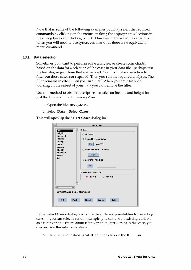
Note that in some of the following examples you may select the required commands by clicking on the menus, making the appropriate selections in the dialog boxes and clicking on OK. However there are some occasions when you will need to use syntax commands as there is no equivalent menu command.
13.1 Data selection Sometimes you want to perform some analyses, or create some charts, based on the data for a selection of the cases in your data file - perhaps just the females, or just those that are married. You first make a selection to filter out those cases not required. Then you run the required analyses. The filter remains in effect until you turn it off. When you have finished working on the subset of your data you can remove the filter.
Use this method to obtain descriptive statistics on income and height for just the females in the file survey2.sav.
1 Open the file survey2.sav.
2 Select Data | Select Cases.
This will open up the Select Cases dialog box.
In the Select Cases dialog box notice the different possibilities for selecting cases — you can select a random sample, you can use an existing variable as a filter variable (more about filter variables later), or, as in this case, you can provide the selection criteria.
3 Click on If condition is satisfied, then click on the If button.
Guide 27: SPSS for UNIX 56

Guide 27: SPSS for UNIX 57
4 In the Select Cases: If dialog box, enter the condition sex='F'
5 Click on Continue.
6 In the Select Cases dialog box click on OK to run the command,
or
Paste to put the corresponding commands (in this case there will be several) into the syntax window where you will have to select the commands and Run them.
Notice the words Filter On in the status bar at the bottom of the data window. This reminds you that the next commands to be run will use only the selected cases. Notice also that you have a new variable called filter_$ that has the value 1 for each case selected, and the value 0 for those cases not selected. This is the filter variable. You may specify an existing numeric variable as a filter variable. Cases that have 0 as the value of the filter variable (or missing) will be excluded from subsequent calculations.
1 Now run the Descriptives command on the variables height and income.
2 Look at the output.
(It's surprising how many people don't look at their output!) You should find that the results are based on the data for the females only.
3 Now turn the filtering off.
You should be able to find out how to do this yourself. Use the online help if necessary!
If you wanted to repeat the analysis on the males only instead of the females, you could repeat the above sequence of commands with sex='M' instead of sex='F'.
13.2 Sorting and splitting files Now consider the situation where you have more than two groups of cases that you want to analyse - say for instance you wanted to calculate some statistics separately on each of the four marital status groups (married, single, widowed, divorced). Clearly the above method of selecting each group in turn, then performing the required analyses could become rather tedious, even with the use of syntax commands. SPSS provides a mechanism for splitting the file according to the values in a particular variable (or variables), and then applying the analysis commands separately to each part of the split file. The split remains in effect until you turn it off.

Use this method to obtain separate histograms of the numbers of children for each of the four marital status groups in the data file.
Make sure that filtering is off, so that you will use all cases in the data file.
1 Select Data | Split File.
This will open up the Split File dialog box.
2 In the Split File dialog box, select Repeat analysis for each group.
3 Select marstat as the Groups Based on: variable.
4 Make sure that Sort the file by grouping variables is selected.
5 Click on OK to run the command,
or
Paste to put the corresponding commands (in this case there will be two) into the syntax window where you will have to select the commands and Run them.
Notice the words Split File On in the status bar at the bottom of the data window. This reminds you that the next commands will be performed separately on each subgroup of cases in the file. If you look at the data in the data window you will see that the cases in the file have been sorted by the value of the marstat variable - all the Ds come first, then the Ms, then the Ss and finally the Ws.
When SPSS processes the subsequent commands, it halts whenever the marstat variable changes and produces a set of results, then carries on with the next group of cases. It is therefore vital that the cases are sorted by the splitting variable. If you look at the command syntax you will see that the appropriate commands have been prepared for you. If you look at the
Guide 27: SPSS for UNIX 58

Guide 27: SPSS for UNIX 59
output you should see a comment to the effect that the sort was carried out successfully.
Note that if the data were already sorted by the variable specified for the grouping, then you could have selected File is already sorted instead of Sort the file by grouping variable in the Split File dialog box. This can save processing time when you have a large datafile. The equivalent in the syntax would have been to omit the Sort command.
1 Now create the charts required, and look at the results!
2 Turn split file processing off.
13.3 Sorting the working data file There may be times when you wish to sort the data in the file without necessarily combining it with a split file command. For instance it may be easier to check some data values if the data are arranged in a particular way.
Sort the data now by the person variable.
1 Select Data | Sort Cases,
or
make a modification to the Sort command in the syntax window and run that.
Look at the data in the data window and check that the data are indeed now sorted by the person scores.
13.4 Saving selected variables only After working with a file for sometime you may wish to save the working data file, but not necessarily save all the variables. Instead of deleting those you don't want to save, you could just save those variables you wish. The unsaved variables will still remain in the working data file, but will not be copied to the SPSS data file. This option is only available using a syntax command. You cannot do this using the menu commands.
Use this method now to make a new SPSS data file with just the data for the variables person, sex, age, marstat and nkids.
Make sure that the data are sorted by person before you do this - see previous section.
You will need a syntax window to save selected variables.
If you haven't been using syntax commands in this session you probably won't have a syntax window open. You can open one by selecting Paste from any dialog box, or you can select File | New | Syntax from the data window.

Guide 27: SPSS for UNIX 60
1 In the syntax window, type the following command: SAVE OUTFILE='survey2a.sav' /KEEP=person, sex, age, marstat, nkids .
Note that when you specify a list of variables that are next to one another in the working data file, you can abbreviate the list using the word to, e.g.
SAVE OUTFILE='survey2a.sav' /KEEP=person to nkids .
Don't forget the command terminator.
2 Run the completed SAVE command.
Note that the working data file is unaffected by this save command. The title in the data window remains unchanged, and all the original variables are still present.
13.4.1 Open a file with selected variables only Sometimes you may have a data file with a large number of variables in it, but you want to perform some analyses based on just a few of those variables. Instead of getting SPSS to read all the data, you could read in just those variables you want to work with. It will be easier to work with the file without the dialog boxes listing variables you will not be using.
The option of specifying which variables you want to read is only available using a syntax command. You cannot do this using the menu commands.
Use this now to open the SPSS data file survey2.sav with just the data for the variables person, income, height and sheight.
1 In the syntax window, type the following command: GET
2 Click on Syntax for information about the option you will need.
3 On the basis of the online help, complete the command specifying survey2.sav as the name for the SPSS data file that you will read, and person, income, height and sheight for the variables you want to keep.
Don't forget the command terminator.
4 Run the completed GET command.
Note that when you use this form of the GET command, the name survey2.sav still appears in the title bar of the data window, even though it only contains some of the variables from that file.
Note also that the data are not actually read into the working data file until you run a procedure that requires the data, or you run an EXECUTE command.
Guide 27: SPSS for UNIX 61
5 Use File | Save As (not File | Save) to save this reduced data file as a new SPSS data file using the filename survey2b.sav
or
Use the syntax command SAVE OUTFILE='survey2b.sav' .
You should now have two new SPSS data files, each containing a subset of the variables from the original file survey2.sav. You will discover shortly how to re-combine these files using a procedure that merges files holding data for the same cases but different variables.
1 Open each of these two files to confirm that each contains all the cases, but a different selection of variables.
As you can only have one data file open at once, SPSS will close the file that's open before opening another one.
13.4.2 Saving selected cases only Sometimes you may wish to create separate SPSS data files for different groups of cases - say the males and the females.
For each subset of cases you require as a separate file, you will need to read the complete file, delete those cases not required, then save what is left as a new file with a different name. The easiest way to do this is to use syntax commands.
Use this to create two new SPSS data files based on the data in survey2.sav, one for the males in the file and the other for the females. Call them survey2m.sav and survey2f.sav.
1 Open the file survey2.sav.
2 In the syntax window, type and run the commands: SELECT IF (SEX='M') . EXECUTE .
This will delete from the working data file those cases that do not satisfy the selection criterion specified.
3 Use File | Save As (not File | Save) to save this reduced data file as a new SPSS data file using the filename survey2m.sav.
4 Use a similar procedure (starting from the command to open survey2.sav) to create a file called survey2f.sav for the data for the females only, and another called survey2x.sav for those with the missing value X for sex.

Guide 27: SPSS for UNIX 62
5 Open each of the three files survey2m.sav, survey2f.sav and survey2x.sav, in turn, to confirm that each contains all the variables, but a different selection of cases.
13.5 Combining files SPSS provides a mechanism for combining data from two or more files. You can merge several files containing data for the same cases but different variables, and you can merge several files containing data for the same variables but different cases. The data to be merged must be in SPSS data files.
13.5.1 Same cases — different variables There may be occasions when you have the data for the same cases in several files, and may wish to bring them together in order to look for relationships between the variables in the different files. For instance you may be conducting a longitudinal study in which you follow up the same cases over a period of time and collect data from them on a number of occasions, or you may be collecting data on your cases from a number of different sources.
You would need to be able to match the cases in one file with those in the other file. This is usually done by having a matching case identifier in each file, and having the data in each file sorted by the identifying variable.
If you have been following all the exercises in these notes then you should have two files survey2a.sav and survey2b.sav that satisfy these criteria. (If you don't have these files, then you can copy them from the /usr/local/courses/spss directory.)
If you use syntax commands, you can combine variables from several files at once. If you use menu commands you can only add data from two files at once. In this case you must first open one of the files, then add to it variables from another file. If you want to merge data from several files, then it is better to use syntax commands.
Whichever method you use, you can specify, from each file, which variables to keep (or which variables to drop). You can also specify which variable in each file to use as the key variable for matching the cases from the several files. Whether you use menus or syntax, the new composite file becomes the new working data file.
You are now going to merge the data from the two files survey2a.sav and survey2b.sav. Try this first using menu commands and dialog boxes, but Paste the commands into a syntax window and Run them from there. This way you will see the equivalent syntax commands.
1 Open the file survey2a.sav.

2 Select Data | Merge Files | Add Variables.
This will open up the Add Variables: Read File dialog box.
3 Choose the file survey2b.sav and click on OK.
This will open up the Add Variables dialog box.
4 Choose which variables you want to include in the new composite file.
Notice that you can exclude variables from either the working data file, or the new file being added.
5 Click on Match cases on key variable in sorted files, and specify person as the Key Variable.
6 Click on Paste.
SPSS will remind you that the data in each file needs to be sorted by the key variable.
7 In the syntax window, select the MATCH FILES command, and the EXECUTE command that follows it, and Run them.
8 Look at the data window and check that you have all the variables and all the cases that you expect.
If you have chosen to keep all the variables from both files, your syntax commands will look like:
Guide 27: SPSS for UNIX 63
Guide 27: SPSS for UNIX 64
MATCH FILES /FILE=* /FILE='survey2b.sav' /BY person. EXECUTE.
You will notice that SPSS actually writes into the command the full path for any files referenced. However, you can omit the path if you wish, and just give the name of each file, provided the files are in the current working directory.
It is not difficult to see what is happening here. Each /FILE subcommand specifies a file to be involved in the merge, /FILE=* is used to indicate the present working data file.
An alternative way of merging the two files survey2a.sav and survey2b.sav which does not require you to read in one of the files first, is to use a modified form of the MATCH FILES syntax command.
1 Modify the syntax commands as follows, and run them: NEW FILE . MATCH FILES /FILE='survey2a.sav' /FILE='survey2b.sav' /BY person . EXECUTE .
Note that using syntax you can add variables from several files at once by including several /FILE subcommands. Up to 50 filenames can be specified on one MATCH FILES command!
It is not necessary to include all the variables from each file when you are combining files with the MATCH FILES command.
1 Create a new file containing just the variables person, sex, age and income by combining just the chosen variables from the files survey2a.sav and survey2b.sav.
You may need to look at the online help to get further details of the MATCH FILES command (or experiment with the Add Variables dialog box), in order to find out about how to keep selected variables only.
13.5.2 Same variables — different cases There may be occasions when you have the data for some cases in one file, and data for further cases, but the same variables, in another file, and you may wish to bring them together in order to analyse the larger data set. For instance you may have started experimenting with the analysis of your data when only a small sample of the full data set was available. Or you may have collected data for different cases on different occasions and have them entered initially into different files.
You would normally have the same variables in each file, but different cases. If you have been following all the exercises in these notes then you

Guide 27: SPSS for UNIX 65
should have three files survey2f.sav, survey2m.sav and survey2x.sav that satisfy these criteria. (If you don't have these files, then you can copy them from the /usr/local/courses/spss directory.)
If you use syntax commands, you can combine cases from several files at once. If you use menu commands you can only add data from two files at once. In this case you must first open one of the files, then add to it cases from one other file. If you want to merge data from several files, then it is better to use syntax commands.
Whichever method you use, the new composite file becomes the new working data file.
Merge the data from the two files survey2f.sav and survey2m.sav. Try this first using menu commands and dialog boxes, but Paste the commands into a syntax window and Run them from there. This way you will see the equivalent syntax commands.
1 Open the file survey2f.sav.
2 Select Data | Merge Files | Add Cases.
This will open up the Add Cases: Read File dialog box.
3 Choose the file survey2m.sav and click on OK.
This will open up the Add Cases dialog box.
4 Choose which variables you want to include in the new composite file.
Notice that you can exclude variables if you wish.
5 Click on Paste.
6 In the syntax window, select the ADD FILES command, and the EXECUTE command that follows it, and Run them.
7 Look at the data window and check that you have all the variables and all the cases that you expect.
If you have chosen to keep all the variables from both files, your syntax commands will look like:
ADD FILES /FILE=* /FILE='survey2m.sav' . EXECUTE.
Note that using syntax you can add cases from several files at once by including several /FILE subcommands up to 50 filenames can be specified on one ADD FILES command!
1 Write and Run a single ADD FILES command to merge the data from the three files survey2f.sav, survey2m.sav and survey2x.sav.

2 Look at the data window and check that you have all the variables and all the cases that you expect.
14 Being in control — SPSS preferences There are several ways in which you can customise SPSS to suit your way of working. For instance you can specify whether or not you want to record all your commands in a journal file, whether or not you want the commands you use to be included in the output, whether you want any areas in your charts to be filled with colours or patterns, and so on.
You can change your preferences for just the current SPSS session, or you can save your preferences and have them effective for subsequent sessions.
1 In the data window, select Options | Preferences.
This will open up the Preferences dialog box.
14.1 Command recording Unless you have already made changes to the default settings, you will see that command recording is on, and that new commands are appended to the journal file. If you click on the File button in the Session Journal box, you will also see that the file spss.jnl in your home directory is used as the journal file. You can change the name of the file to use as the journal file. You can also change the other settings. The following table indicates what effect changing these settings will have:
Journal Status Outcome off No commands are recorded. on overwrite Commands are always recorded.
A new journal file is created for each SPSS session. Any previous journal file is deleted.
on append Commands are recorded only if journal file exists.
Guide 27: SPSS for UNIX 66
Guide 27: SPSS for UNIX 67
Commands added to the end of the journal file. If journal file doesn't exist, commands are not recorded.
Click on the appropriate buttons in the Session Journal box to make whatever changes you wish.
14.2 Graphics options Click on the Graphics button to open the Preferences: Graphics dialog box. This will allow you to alter some of the defaults that are used when you create charts.
Make any changes you wish, then click on Continue.
14.3 Output options
1 Click on the Output button to open the Preferences: Output dialog box. This will allow you some control over the layout and content of the output produced by SPSS.
2 Make any changes you wish, then click on Continue.
14.4 Saving preference settings
1 When you are finished making changes, click on OK in the Preferences dialog box.
The changes will be effective throughout the remainder of the current SPSS session.
2 If you want the changes to be effective for future SPSS sessions, select Options | Save Settings in the data window.
If you don't save the preferences, then when you exit from SPSS, you will be asked whether or not you want to save the changed preferences settings.
15 Portability SPSS is available for many different types of computer. At the University of Durham, both UNIX and PC (Microsoft Windows) versions are available.
There may be times when you want to transfer your work from one system to another.
15.1 Command files Although there are some differences in the way SPSS commands are run on different systems, the syntax of the commands is essentially the same for all systems. This means that an SPSS program written for one system should transport with little difficulty to another system. Some details may need to be changed. For instance the rules for the naming of files vary between

Guide 27: SPSS for UNIX 68
systems, and so any file names referenced in a program may need to be changed. Also there are some commands which are available on some systems but not others.
15.2 SPSS data files SPSS data files are usually system specific. This means that an SPSS data file written on one system will probably not be able to be read by SPSS on another system. However, the UNIX version of SPSS (version 5.0) will read SPSS data files created by SPSS for UNIX version 4.0, and by SPSS for Windows (version 9.0); and SPSS for Windows can read SPSS data files created by the UNIX version of SPSS. Note that SPSS data files are not text (ASCII) files and must be transferred from one system to the other in binary mode (not text mode).
It is also possible to transfer SPSS files from one system to another using SPSS portable files. SPSS portable files are text files, and should be transferred from one system to another is the same way as you would transfer any other text file. All versions of SPSS have the ability to save the working data file as an SPSS portable file, and all versions of SPSS have the ability to import an SPSS portable file.
15.3 Chart files Chart files are system specific. This means that charts created on one system cannot be read by SPSS running on a different system.
16 Further information
16.1 ITS documents The following documents are available from the ITS Helpdesk.
Guide 167: Copying material from SPSS to Microsoft Word 2002 (Office XP) This guide explains how you can copy data and output (including charts) from SPSS for Windows into a Word for Windows document.
Guide 86: SPSS for Windows - Importing and Exporting Data This guide explains in detail how to copy data from Excel, Word and Access into SPSS, and vice versa.
Guide 32: SPSS for Windows These notes provide an introduction to the PC version of SPSS.
16.2 SPSS manuals The following SPSS manuals give full details of the UNIX version of SPSS.

Guide 27: SPSS for UNIX 69
SPSS for UNIX Base System User's Guide Release 5.0: 0-13-107145-9 This provides detailed information on how to run SPSS using the window manager. It also explains many of the statistical concepts involved, how to use the procedures correctly, and how to interpret the results.
SPSS Base System Syntax Reference Guide Release 5.0: 0-13-177668-1 This documents, and provides examples of, all the command syntax in the Base system. Although most of the facilities of the Base system are available using the CDE interface, there are some that can only be obtained by entering and running syntax commands.
SPSS for UNIX Professional Statistics: 0-13-107152-1 This documents the procedures available in the SPSS Professional Statistics system. It includes cluster analysis, discriminant analysis, factor analysis, multidimensional scaling, and so on.
SPSS for UNIX Advanced Statistics: 0-13-107137-8 This documents the procedures available in the SPSS Advanced Statistics system. It includes sophisticated techniques such as logistic regression, loglinear analysis, multivariate analysis of variance, probit analysis, and so on.
SPSS manuals are available in the University Library, and, for reference only, in the ITS Helpdesk, Computer Centre.
16.3 Other documents
SPSS Guide to Data Analysis: 0-918469-42-2 This includes sections on preparing data for analysis, describing data, hypothesis testing and examining relationships in data.
16.4 Help and advice For questions and advice about all computing matters, the ITS Helpdesk is available:
• by personal contact in the Helpdesk in the Computer Centre (9.00am – 6.00pm, Monday to Friday)
• by telephone (41515), hours as above. • by electronic mail to [email protected]. Messages are
normally answered during the same day.
16.5 Formic If you use paper based forms or questionnaires there is an automated questionnaire system available in the ITS. The system is called Formic, a Windows based package that can be used to design and create paper forms that can subsequently be scanned in automatically. The results are then

Guide 27: SPSS for UNIX 70
stored in a database file which can be exported in a number of different formats (e.g. Excel, Access or SPSS). The system works best with ‘tick boxes’, but can be also be used to read handwritten text.
Any member of staff may apply to be registered as a Formic user. Registration as Formic users will only be granted to undergraduates and postgraduates with genuine academic projects which are approved and supported by a member of staff. Applications should be made direct to the Helpdesk (e-mail [email protected], or phone 41515).

Guide 27: SPSS for UNIX 71
Appendix A: Increasing the size of the text in the windows
If you find that the text in the windows and dialog boxes is rather small, then you might like to know how you can make it larger. One way of doing this is to include appropriate commands in a file called .Xdefaults in your home directory.
An example of such commands are in the file /usr/local/courses/spss/bigfonts. You can add these commands to your .Xdefaults file as follows:
At a UNIX prompt, type
cd cat /usr/local/courses/spss/bigfonts >> .Xdefaults
If you already had a .Xdefaults file, then the larger characters will be used the next time you run SPSS.
If you did not have a .Xdefaults file before, then the larger characters will not become available to SPSS until the next time you run Xwin to start up CDE.
Note that these larger fonts will also be used when you print from a text window (data, output or syntax) using PostScript. They will not affect ASCII printing.
If you wish to revert to standard size fonts, type the following at the UNIX prompt:
cd
cat /usr/local/courses/spss/standardfonts >> .Xdefaults
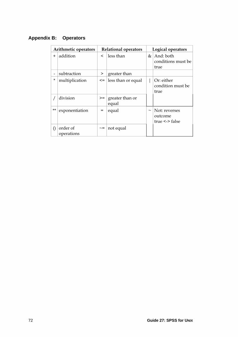
Guide 27: SPSS for UNIX 72
Appendix B: Operators
Arithmetic operators Relational operators Logical operators + addition < less than & And: both
conditions must be true
- subtraction > greater than * multiplication <= less than or equal | Or: either
condition must be true
/ division >= greater than or equal
** exponentiation = equal ~ Not: reverses outcome true <-> false
() order of operations
~= not equal

Guide 27: SPSS for UNIX 73
Appendix C: Answers to selected exercises
The following solutions are suggested for some of the exercises. Note that there will often be several ways of achieving the desired result, all of which may be equally valid. It does not matter if your solution is different from the one offered here so long as it works!
Section 10.2 (using functions)
newvar=mean.1(height,sheight)
or
newvar=mean(height,sheight)
Section 10.4 (conditional compute commands)
1. marstat = ‘M’ & nkids > 0 2. marstat = ‘M’ & nkids = 0 3. marstat ~= ‘M’ & nkids > 0 4. marstat ~= ‘M’ & nkids = 0
Section 10.6 (conditional recode commands)
1) Using RECODE recode height into tall – need to do this in two steps: 1 Condition: sex='F', values: lowest through 67.9 → 0,
68 through highest → 1, missing → missing
2 Condition: sex='M', values lowest through 71.9 → 0, 72 through highest → 1, missing → missing
2) Using COMPUTE again use two steps, with same newvar (tall2) each time
1 value=0, condition: (sex = 'F' & height < 68) or (sex = 'M' & height < 72)
2 value=1, condition: (sex = 'F' & height >= 68) or (sex = 'M' & height >= 72)
3) Obtain summary statistics for both variables you should get identical results if the two variables are the same. Use the COMPUTE command to create a new variable based on the difference between the two variables to be tested (e.g. tall-tall2). If the two variables are the same then the difference variable should have the value zero (or missing) for all cases.
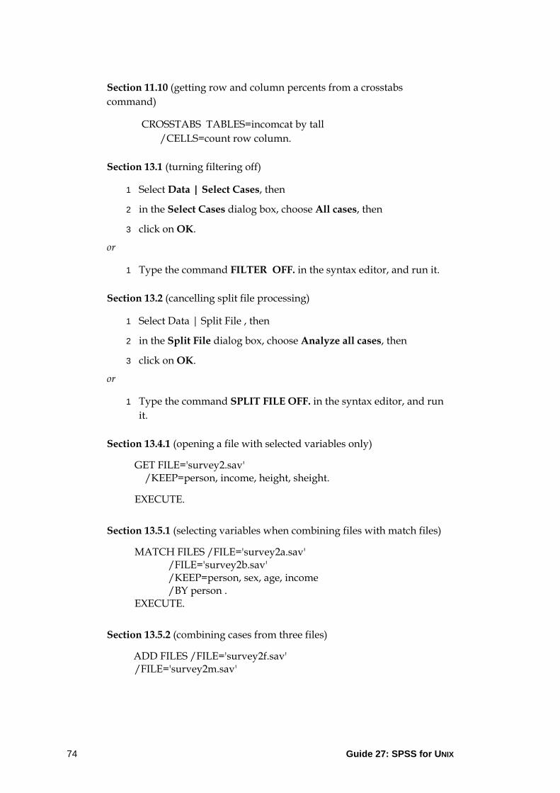
Guide 27: SPSS for UNIX 74
Section 11.10 (getting row and column percents from a crosstabs command)
CROSSTABS TABLES=incomcat by tall /CELLS=count row column.
Section 13.1 (turning filtering off)
1 Select Data | Select Cases, then
2 in the Select Cases dialog box, choose All cases, then
3 click on OK.
or
1 Type the command FILTER OFF. in the syntax editor, and run it.
Section 13.2 (cancelling split file processing)
1 Select Data | Split File , then
2 in the Split File dialog box, choose Analyze all cases, then
3 click on OK.
or
1 Type the command SPLIT FILE OFF. in the syntax editor, and run it.
Section 13.4.1 (opening a file with selected variables only)
GET FILE='survey2.sav' /KEEP=person, income, height, sheight.
EXECUTE.
Section 13.5.1 (selecting variables when combining files with match files)
MATCH FILES /FILE='survey2a.sav' /FILE='survey2b.sav' /KEEP=person, sex, age, income /BY person . EXECUTE.
Section 13.5.2 (combining cases from three files)
ADD FILES /FILE='survey2f.sav' /FILE='survey2m.sav'

Guide 27: SPSS for UNIX 75
/FILE='survey2x.sav'. EXECUTE.
Appendix D: Recommended naming conventions for different types of files
extension used for text file? print with lp? cat to screen? .dat ASCII data file yes yes yes .sav SPSS data file .sps SPSS command file yes yes yes .lst SPSS output listing yes yes yes .cht SPSS chart file
SPSS data files (.sav) and SPSS chart files (.cht) are in a special format that only SPSS can read. You should not attempt to list, edit or print these files.