Embed Size (px)
Citation preview
SANDIA REPORT SAND86-2994· DOE/HWP-26. UC-69 Unlimited Release Printed May 1988
"
SRS: Site Ranking System for Hazardous Chemical and Radioactive Waste
Rob P. Rechard, Margaret S. Y. Chu, Stephen L. Brown
Prepared by Sandia National Laboratories Albuquerque, New Mexico 87185 and Livermore, California 94550 for the United States Department of Energy under Contract DE-AC04-76DP00789
SF2900Q(8-81 J
When printing a copy of any digitized SAND Report, you are required to update the
markings to current standards.
Issued by Sandia National Laboratories, operated for the United States Department of Energy by Sandia Corporation. NOTICE: This report was prepared as an account of work sponsored by an agency of the United States Government. Neither the United States Govern- ment nor any agency thereof, nor any of their employees, nor any of their contractors, subcontractors, or their employees, makes any warranty, express or implied, or assumes any legal liability or responsibility for the accuracy, completeness, or usefulness of any information, apparatus, product, or process disclosed, or represents that its use would not infringe privately owned rights. Reference herein to any specific commercial product, process, or service by trade name, trademark, manufacturer, or otherwise, does not necessarily constitute or imply its endorsement, recommendation, or favoring by the United States Government, any agency thereof or any of their contractors or subcontractors. The views and opinions expressed herein do not necessarily state or reflect those of the United States Government, any agency thereof or any of their contractors or subcontractors.
Printed in the United States of America Available from National Technical Information Service US . Department of Commerce 5285 Port Royal Road Springfield, V A 22161
NTIS price codes Printed copy: A13 Microfiche copy: A01
*ENVIRON Corporation, Washington, DC
SAND86-2994 DOE/HWP-26 Unlimited Release, UC-69
SRS: SITE RANKING SYSTEM FOR HAZARDOUS CHEMICAL AND RADIOACTIVE WASTE
Rob P. Rechard Margaret S . Y. Chu Stephen L. Brown*
Prepared March 1987 Printed May 1988
Waste Management Systems Division Sandia National Laboratories
Albuquerque, New Mexico 87185
Sponsored by the U.S. DOE Hazardous Waste Remedial Actions Program
through the Support Contractor Office
Oak Ridge, Tennessee 37831 operated by
Martin Marietta Energy Systems, Inc.
PREVIOUS DOCUMENT IN SERIES
Chu, M. S . Y., J. V. Rodricks, C. St. Hilaire, and R. L. Bras, 1986. Risk assessment and ranking methodologies for hazardous chemical defense waste: A state-of-the-art review and evaluation, Task 1 Report, SAND86-0530, Sandia National Laboratories, Albuquerque, NM 87185.
ACKNOWLEDGEMENTS
We appreciate the time and suggestions supplied by the technical reviewers: R. L. Hunter, R. M. Ostmeyer, and D. Tomasko of Sandia National Laboratories and J. Vandevan of ENVIRON Corporation. In addition, we acknowledge the help of C. St. Hilaire of Risk Science Institute, J. V. Rodricks of ENVIRON, P. A . Rechard of Western Water Consultants, and J. C . Helton of Arizona State University in the early stages of this report. Development of SRS was funded by the Hazardous Waste Remedial Action Program (HAZWRAP) of the Department of Energy (DOE). We thank H. F. Bauman and J. Petty of Martin Marietta Energy Systems, Inc, Oak Ridge, TN for their managerial support.
- 4 -
ABSTRACT
This report describes the rationale and presents instructions for a Site - ranking System ( S R S ) . SRS ranks hazardous chemical and radioactive waste sites by scoring important and readily available factors that influence risk to human health. Using SRS, sites can be ranked for purposes of detailed site investigations. SRS evaluates the relative risk as a combination of potentially exposed population, chemical toxicity, and potential exposure of release from a waste site; hence, SRS uses the same concepts found in a detailed assessment of health risk. Basing SRS on the concepts of risk assessment tends to reduce the distortion of results found in other ranking schemes. More importantly, a clear logic helps ensure the successful application of the ranking procedure and increases its versatility when modifications are necessary for unique situations. Although one can rank sites using a detailed risk assessment, it is potentially costly because of data and resources required. SRS is an efficient approach to provide an order-of-magnitude ranking, requiring only readily available data (often only descriptive) and hand calculations. Worksheets are included to make the system easier to understand and use.
-5- 6 -
CONTENTS
Page
. .~
-
.
.
.
..
.
.
.
I
.
.
.
..
1 . SUMMARY . . . . . . . . . . . . . . . . . . . . . . . . . . . . . 1 3
2 . INTRODUCTION . . . . . . . . . . . . . . . . . . . . . . . . . . 1 9
Organization of Report . . . . . . . . . . . . . . . . . . . . . 1 9 Using this Report . . . . . . . . . . . . . . . . . . . . . . . . 1 9 ObjectiveofSRS . . . . . . . . . . . . . . . . . . . . . . . . 20 Background on DOE Hazardous Waste Program . . . . . . . . . . . . Juxtaposition of SRS to other Waste Site Decisions . . . . . . . 2 4 SNLA Proposed Risk Methodology . . . . . . . . . . . . . . . . . 27 Review of Ranking Methods . . . . . . . . . . . . . . . . . . . . Incidents from Waste Disposal Sites . . . . . . . . . . . . . . . 35
3 . GENERAL ASPECTS OF SRS . . . . . . . . . . . . . . . . . . . . . 37
2 1 22 Relationship of SRS to Risk Assessment and Risk Management . . .
30
OverviewofSRS . . . . . . . . . . . . . . . . . . . . . . . . . 37 Principles Guiding Development of SRS . . . . . . . . . . . . . . 4 0 Scoring Concept of SRS . . . . . . . . . . . . . . . . . . . . . 42 Scoring Individual Factors . . . . . . . . . . . . . . . . . . . 45 Sensitivity/Uncertainty Analysis . . . . . . . . . . . . . . . . 47 Sensitivity of Variables in SRS . . . . . . . . . . . . . . . . . 48 Uncertainty Analysis in SRS . . . . . . . . . . . . . . . . . . .
Summary of SRS Assumptions . . . . . . . . . . . . . . . . . . . 5 4
50 Using Monitoring Data . . . . . . . . . . . . . . . . . . . . . . 53
4 . POPULATION AND TOXICITY SCORES . . . . . . . . . . . . . . . . . 55
Population . . . . . . . . . . . . . . . . . . . . . . . . . . . 55 Chronic Toxicity . . . . . . . . . . . . . . . . . . . . . . . . 56
5 . GROUND-WATER SCORE . . . . . . . . . . . . . . . . . . . . . . . 61
Idealized Ground-Water Pathway . . . . . . . . . . . . . . . . . 61 Method of Scoring . . . . . . . . . . . . . . . . . . . . . . . . 62
ModelEquation . . . . . . . . . . . . . . . . . . . . . . . . . 7 3 Model Sensitivity . . . . . . . . . . . . . . . . . . . . . . . . 7 5
Derivation of Scoring Model . . . . . . . . . . . . . . . . . . . 64
6 . SURFACE-WATER SCORE . . . . . . . . . . . . . . . . . . . . . . . 78
Idealized Surface-Water Pathway . . . . . . . . . . . . . . . . . 7 8 Method of Scoring . . . . . . . . . . . . . . . . . . . . . . . . 7 9 Derivation of Scoring Model . . . . . . . . . . . . . . . . . . . 82
7 . AIRSCORE . . . . . . . . . . . . . . . . . . . . . . . . . . . . 88
Idealized Air Pathway . . . . . . . . . . . . . . . . . . . . . . 88 Method of Scoring . . . . . . . . . . . . . . . . . . . . . . . . 88 Derivation of Scoring Model . . . . . . . . . . . . . . . . . . . 91
- 7 - -"
- I_--- ....... .. ................
CONTENTS (continued)
Page
8 . SITE RANKING SYSTEM (SRS) INSTRUCTIONS . . . . . . . . . . . . . 99
Conventions Observed in the Instructions . . . . . . . . . . . . 99 OverviewofSRS . . . . . . . . . . . . . . . . . . . . . . . . . 99 General Scoring Guidelines . . . . . . . . . . . . . . . . . . . 102 Site Ranking Procedure . . . . . . . . . . . . . . . . . . . . . 102
Step 1: Collect data on waste properties . . . . . . . . . . 1 0 4
Step 3: Describe release pathways . . . . . . . . . . . . . . 111 Step 4: Evaluate engineered features . . . . . . . . . . . . 115 Step 5: Identify target populations . . . . . . . . . . . . . 119 Step 6: Score site factors . . . . . . . . . . . . . . . . . 121
Step 2: Score and rank chemicals found at site . . . . . . . 105
Step 6.G1: Score ground-water dilution . . . . . . . . 122 Step 6.G2: Score ground-water mass adjustment . . . . 129 Step 6.S1: Calculate dilution for surface water . . . 134 Step 6.S2: Score surface-water mass adjustment . . . . 138 Step 6.S3: Score surface-water sediment yield . . . . 141 Step 6.A1: Assume mass-release adjustment . . . . . . 146 Step 6.A2: Calculate mass-release adjustment . . . . . 147
Step 7: Combine chemical scores . . . . . . . . . . . . . . . 151 Step 8: Construct ranked list of waste sites . . . . . . . . 152
9 . COMPARISON OF SRS WITH OTHER ASSESSMENT SCHEMES . . . . . . . . . 153
Three Hypothetical Sites Contaminating Ground Water . . . . . . . 153 Hypothetical Site Affecting Air Quality . . . . . . . . . . . . . 160 Comparison of SRS with EPA Rapid Assessment Technique . . . . . . 162
10 . APPENDIX A.. SRS Worksheets . . . . . . . . . . . . . . . . . . . 169
11 . APPENDIX B.. SRS Applied to a Superfund Site . . . . . . . . . . . 189
12 . APPENDIX C.. Chemical Properties of Waste . . . . . . . . . . . . 231
13 . APPENDIX D.. Data Required . . . . . . . . . . . . . . . . . . . . 273
14 . APPENDIX E.. Nomenclature . . . . . . . . . . . . . . . . . . . . 279
15.REFERENCES. . . . . . . . . . . . . . . . . . . . . . . . . . . 287
- 8 -
ILLUSTRATIONS
. ..
-,-
I
Page Figure
2.1 Juxtaposition of SRS ranking with other waste site decisions. . . . . . . . . . . . . . . . . . . . . . . 25
2.2 SNLA's modular method of assessing risks from hazardous waste disposal . . . . . . . . . . . . . . . 28
2.3 Potential contaminant movement that could be important to simulate in consequence modeling . . . . . . . . . , . . 29
3 . 1 The three simplified pathways examined in SRS . . . . . . . 38
3.2 Diagram of SRS Procedure. . . . . . . . . . . . . . . . . . 39
5.1 Conceptual model for ground-water pathway . . . . . . . . . 62
5.2 Variation of dispersivity with distance . . . . . . . . . . 71
6.1 Conceptual model for surface-water pathway. . . . . . . . . 79
7 . 1 Conceptual model for air pathway. . . . . . . . . . . . . . 89
8.1 General pathways examined in SRS. . . . . . . . . . . . . . 1 0 1
8.2 Diagram of SRS procedure. . . . . . . . . . . . . . . . . . 103
8.3 Conceptual model and definition of terms for ground-water pathway. . . . . . . . . . . . . . . . . . 113
8.4 Conceptual model and definition of terms for surface-water pathway . . . . . . . . . . . . . . . . . 114
8.5 Conceptual model and definition of terms for air pathway . . . . . . . . . . . . . . . . . . . . . . 1 1 4
8.6 Mean annual rainfall in United States . . . . . . . . . . . 126
8.7 Mean annual rainfall-erosivity factor in United States. . . 144
8.8 Length-slope topographic factor . . . . . . . . . . . . . . 145
8.9 Map of PE index for United States . . . . . . . 1 . . . . . 150
8.10 Juxtaposition of SRS ranking with other waste site decisions. . . . . . . . . . . . . . . . . . . . . . . 152
- 9 -
TABLES
Page Tab 1 e
2 . 1
4 . 1
4 . 2
5.1
5 . 2
8 . 1
8 . 2
8 . 3
8 . 4
8 . 5
8 . 6
8 . 7
8 . 8
8 . 9
8 .10
8 . 1 1
8 .12
8 . 1 3
8 . 1 4
8 .15
8.16
8.17
8 .18
8 .19
Pathway by which industrial disposal sites caused environmental hazard . . . . . . . . . . . . . . . . . . . . 36
Target population scores . . . . . . . . . . . . . . . . . . 55
Chemical/radionuclide chronic toxicity . . . . . . . . . . . 60
Dispersivities reported in the literature . . . . . . . . . 73
Influence of variables as represented by power [b.] in ground-water equation . . . . . . . . . . . . 77
Scores for waste quantity . . . . . . . . . . . . . . . . . 108
1
Volumes of common waste containers . . . . . . . . . . . . . 108
Chemical/radionuclide chronic toxicity . . . . . . . . . . . 109
Scores for source decay . . . . . . . . . . . . . . . . . . 109
Qualitative descriptions of decay rates . . . . . . . . . . 110
Scores for solubility . . . . . . . . . . . . . . . . . . . 110
Waste placement scores for all routes . . . . . . . . . . . 116
Leachate reduction for ground-water route . . . . . . . . . 1 1 7
Leachate collection system for ground-water route . . . . . 117
Protection of waste from surface runoff . . . . . . . . . . 118
Target-population scores . . . . . . . . . . . . . . . . . . 119
Score for distance to population for ground-water route . . . . . . . . . . . . . . . . . . . 120
Score for distance to population for air route . . . . . . . 120
Fraction of precipitation percolating into waste . . . . . . 124
Hydraulic conductivity for various rock types . . . . . . . 125
Range of porosity for various rock types . . . . . . . . . . 125
Scores for aquifer fluid velocity in pores . . . . . . . . . 127
Scores for aquifer thickness . . . . . . . . . . . . . . . . 127
Ground-water route dilution scores . . . . . . . . . . . . . 128
-10-
TABLES (continued)
Table
8.20
8 . 2 1
8 .22
8 . 2 3
8 .24
8 . 2 5
8 .26
8 .27
8 .28
8 .29
8 .30
8 . 3 1
8 .32
9 . 1
9 . 2
9 . 3
9 . 4
9 . 5
9 . 6
9 . 7
9 . 8
9 . 9
9 .10
Page
Mass-release adjustment scores for ground-water route . . . 130
Scores for retardation in ground-water. . . . . . . . . . . 133
Fraction of organic matter of soil in several areas of the United States. . . . . . . . . . . . . . . . . 133
Definition of SCS hydrologic soil groups. . . . . . . . . . 136
Scores for runoff . . . . . . . . . . . . . . . . . . . . . 136
136 $7.Vr-rn--,-7*C.- .- . - i d .... c - . . . . . . . . . . . . . .
Runoff curve numbers for selected agricultural, suburban, and urban land use. . . . . . . . . . . . . . . . 137
Mass-release adjustment for surface-water route . . . . . . 139
Scores for runoff dissolution . . . . . . . . . . . . . . . 140
Control-practice factor [CP] for pasture, rangeland, andwoodland. . . . . . . . . . . . . . . . . . . . . . . . 142
Sediment yield from drainage area of 100 mi or less in the United States. . . . . . . . . . . . . . . . 143
2 ( 2 . 6 ~ 1 0 ~ m 2 )
Scores for surface-water sediment yield . . . . . . . . . . 143
Mass-release adjustment of air route. . . . . . . . . . . . 149
Data general to three hypothetical sites. . . . . . . . . . 154
Data specific to site 3 . . . . . . . . . . . . . . . . . . 155
SRS chemical score for sites 1, 2 , and 3 . . . . . . . . . . 156
Scores unaffected by chemical type at three sites . . . . . 157
Ground-water scores for sites 1, 2 , and 3 . . . . . . . . . 158
Relative health risks as scored by SRS, RAPS, HRS, and mHRS. . . . . . . . . . . . . . . . . . 159
SRS chemical score for PCB site . . . . . . . . . . . . . . 161 Scoring of PCB site . . . . . . . . . . . . . . . . . . . . 161
Comparison of SRS with rapid assessment technique for air pathway . . . . . . . . . . . . . . . . . 162
Data for CC14 site. . . . . . . . . . . . . . . . . . . . . 163
I -11-
.......... lll_l-ll__l_ll_ll_l" I__1_. ........................ _. _"I. I_
Table
TABLES (continued)
Page
9.11
9.12
9.13
9.14
c.1
c.2
c . 3 c.4
c.5
C . 6
c.7
SRS chemical score for CC14 site . . . . . . . . . . . . . . 164
Scores for C C 1 site unaffected by chemical type . . . . . . 165 4 Ground-water scores for CC14 site . . . . . . . . . . . . . 166
Comparison of SRS with rapid assessment technique for ground-water pathway . . . . . . . . . . . . . 167
U C R toxicity data for radionuclides . . . . . . . . . . . . 239
Physical. chemical. and fate data for hazardous wastes . . . 241
Half-lives of waste in various media . . . . . . . . . . . . 247
AD1 toxicity data for noncarcinogens . . . . . . . . . . . . 253
U C R toxicity data for chemical carcinogens . . . . . . . . . 261
EPA categories for potential carcinogens . . . . . . . . . . 263
Estimated carcinogenic potency factors (CPFs ) . . . . . . . 264
- 1 2 -
1. SUMMARY
Purpose of SRS
The site ranking system (SRS) is a method for ranking waste sites containing hazardous chemicals and radionuclides using readily available site data. SRS ranks each individual site by scoring factors that influence the human health risk. Using SRS, one can group waste sites into those that need more detailed study of risk for remedial action and those that do not. In addition, one finds the approximate order to begin investigating sites for detailed risk assessments, remedial investigations (RI), and feasibility studies (FS). In short,
The purpose of SRS is to rank hazardous waste sites according to the relative human health risk they pose. Combining this technical ranking with other risk management criteria, a manager can decide on the best order to begin site investigations and/or actions.
The Need for SRS
In the United States, many waste sites exist, yet the hazards they pose may differ by orders of magnitude. Although one can select sites that pose the greatest public health risk using detailed risk assessment or extensive site monitoring, these approaches are quite costly. Consequently, there is the need for a simple, low-cost approach to provide an order-of-magnitude ranking of sites (similar to that obtained with a detailed risk assessment). SRS satisfies this need. With SRS, the sites with the greatest health risk should appear near the top and those with the least risk near the bottom of the list.
Currently, the most widely used ranking scheme, the Hazard Ranking System (HRS) used by the U.S. Environmental Protection Agency (EPA), has drawbacks (Chu et al., 1986), many of which SRS corrects. In contrast to HRS, SRS
uses a more accurate measure of chemical toxicity
handles both chemical and radioactive hazardous wastes
-13-
evaluates the health hazard from the quantity of each constituent comprising the waste
more adequately evaluates the risk from surface-water runoff
considers ground-water-flow direction and distance
evaluates the potential hazard from the air pathway even without observed releases
does not use arbitrary maximum distances to targets of concern
accounts for environmental attenuation of the hazardous material
separates risk assessment from risk management
The reauthorization of Superfund in October 1986 (SARA, 1986) has required EPA to address several of the above problems with HRS. Thus, developing an improved ranking system such as SRS is also a legislative requirement.
Method for Scorine: Sites
The SRS procedure described in this report scores important and readily available factors that influence the risk to humans. Specifically, SRS measures the risk of a release from a waste site as a combination of the potentially exposed population, the average amount of exposure to the waste, and the toxicity of the waste:
Health Risk a Population Exposure Toxicity
Both the population and the toxicity of each hazardous substance are easily indexed with single scores. Only exposure must be subdivided further into component factors.
In SRS, the specific factors used to evaluate exposure vary with the manner of release. Yet generally, the amount of exposure is evaluated from the mass of material initially deposited at the site [W 1 , a factor indexing the effectiveness of engineered barriers [f 1 , and a factor indexing the ability of site features [fsite] to reduce the amount of hazardous material reaching the potentially exposed population:
0
eng
eng fsite Exposure a Wo f
-14-
When scoring a site, the var.ious factors will likely be known within only a factor of ten; consequently, SRS is simplified by using the logarithms
of the parameters rounded to the nearest integer, which become the "scores."
Combining these scores produces the overall site score.
Rationale for SRS
Several principles and goals guided our development of SRS: SRS was to
approximate the ranking obtained with a detailed risk assessment,
have a logic easy to understand and use,
-- use readily available site data,
require only data that have an order-of-magnitude effect on the health risk (consistent with the uncertainty of preliminary data),
be applicable to most waste sites.
c.
The approach described under "Method of Scoring" is based on the techniques used in detailed assessment of health risk. For this reason, SRS provides an approximation of the ranking obtained with a detailed risk assessment, yet uses preliminary data (often only descriptive) and simple models, permiting hand calculations. This logical basis in risk methodology helps reduce the distortion of the scores--an advantage over many other ranking schemes. More importantly, the clear logic helps in successfully applying SRS in normal and unique situations. For example, if the analyst understands the framework, he can confidently modify SRS for unique situations.
In addition, although a ranking system based on risk assessment could incorporate relatively detailed models (for example, a detailed transport model), the uncertainty of preliminary data (for example, uncertainty in amount of hazardous material) easily swamps the added precision of the model. Furthermore, the more precise model usually requires more data. Thus, we used simple models that captured the most important effects consistent with the accuracy of preliminary site and waste data.
-15-
AssumDtions of the Ranking System
Although numerous assumptions were made in developing SRS, eight assumptions greatly influenced its development. These are as follows
Human health risk is the most important risk to evaluate. Sensitive biological habitats or economic institutions at risk are noted in the narrative accompanying the SRS ranking but are not scored.
The health risk of a hazardous material is adequately determined by scoring its toxicity, the population exposed, and the level of exposure. Acute hazards from flammable and explosive chemicals are described but are not scored.
Scores based on the exposed population rather than an exposed individual are more useful for ranking. (However, the individual exposure is easily evaluated by omitting the population score.)
The health risk posed by a site is best evaluated by chronic (long- term) risks. Although the health risk is a combination of both chronic and acute risks, SRS only evaluates chronic risk because acute risks usually involve emergency rather than remedial response.
The scores for toxicity, population, and exposure are based on best estimates of parameters, not worst-case estimates.
With preliminary site data, only an order-of-magnitude approximation of the health risk and resulting ranking is possible.
The level of exposure can be represented by three generic release pathways: ground water, surface water, and air.
Hazards from direct contact are sufficiently estimated by air pathway.
Svnopsis of Instructions
Ranking hazardous waste sites involves the following eight steps. These steps are presented in detail in Chapter 8 .
1. Collect data on material present at the site. The quantity and toxicity of the hazardous material placed at the waste site directly influences potential health risk; consequently, the chemicals present and their properties are important data. The challenging and time-consuming portion of SRS is the collection of these data.
2. Rank material found at site. This step identifies the substances that are likely to dominate the health risk score. Although in principle the analyst should investigate every substance present, chemicals present in very small quantities, chemicals with very low toxicity, and chemicals that degrade very rapidly may not appreciably affect the overall site risk and thus may be neglected.
-16-
e
3 . Describe release pathways. SRS uses three generic pathways: air, surface water, or ground water; however, SRS also briefly documents the presumed real pathways at the site as part of the ranking procedure. Unusual pathways or conditions that are not treated by SRS can at least be noted in an accompanying narrative.
Steps 4 and 5 score factors pertinent to each pathway.
4. Identify target populations for selected pathways.
5. Evaluate engineered barriers at the site. the site is evaluated specifically for each pathway in this step. Engineered barriers serve to extend the containment of the chemical, lower the release rate, and minimize access to the chemical. They do not, however, provide indefinite isolation.
The engineered design of
The instructions for step 6 are specific to each pathway. But, in general, the instructions break the step into two parts: (1) scoring characteristics applicable to all wastes at the site, and (2) scoring characteristics specific to each waste. As an example, the steps for the ground-water pathway (G1 and G2) are listed.
6.G1 Score ground-water dilution, aquifer velocity, and aquifer thickness.
6.G2 Score ground-water quantity, decay, and retardation adjustments. 7. Evaluate site score. Evaluating the site score consists of first
evaluating each pathway score and then combining the pathway scores
8. Construct ranked list of waste sites. Ordering the sites on the basis of their rank (roughly estimated health risk) is straightforward; however, circumstances such as lack of high quality data may need to be taken into account to differentiate between sites with nearly identical scores.
BackPround on Risk Assessment Proiect -
SRS was developed for use by the Hazardous Waste Remedial Actions Program (HAZWRAP) on hazardous defense waste generated by the U.S. Department of Energy (DOE). DOE, through the HAZWRAP Support Contractor Office, Martin Marietta Energy Systems, Oak Ridge, TN, contracted with Sandia National Laboratories, Albuquerque (SNIA) to develop tools and procedures (a "methodology") for performing risk assessment. The methodology should assist DOE in identifying problems and evaluating solutions for existing and future waste sites; in other words, it should effectively allocate cleanup resources.
-17-
SNLA divided the risk-assessment development task into four subtasks:
1. Evaluation of current techniques for ranking waste disposal sites (reported by Chu et al., 1986);
2. Development of a scheme, based on risk methodology, that ranks DOE hazardous chemical and radioactive waste sites (reported herein);
3 . Development of tools and procedures for a comprehensive risk assessment of DOE disposal sites;
4 . Demonstration and transfer of the methodology to DOE
Subtasks 3 and 4 were proposed but postponed indefinitely because the DOE HAZWRAP program is now oriented toward demonstrating innovative clean-up techniques.
Suggested Future Work
Scoring schemes, by nature, are imperfect tools. Although SRS has a sound logical basis, it undoubtedly has hidden faults that need to be corrected. Consequently, SRS needs to be tested to ensure a good scoring scheme. We recommend
testing the feasibility and credibility of the SRS scoring with at least five real sites--preferably sites that had been thoroughly studied and possibly ranked using another scheme.
performing an analysis of the SRS ranking scheme to examine the sensitivity of the ranking to various input factors and to identify specific improvements needed in SRS,
After carrying out these recommendations, SRS will be ready to rank hazardous waste sites; however, to make SRS even easier to apply, we also recommend
compiling pertinent chemical property data to construct a data base for use with SRS,
placing SRS on a personal computer,
incorporating sensitivity/uncertainty techniques in a computer version.
Suggested related work includes
developing separate ranking scheme for evaluating environmental risks (based primarily on risk indicies)
developing risk-based decision scheme for RCRA-type problems
- 1 8 -
-.-
2. INTRODUCTION
-
-.-
_I
Organization of Report
This report is divided into two major sections: The first section describes the rationale behind the site ranking system (SRS); the second, its use. The first section includes
background information and motivation for developing SRS (remainder of Chapter 2, Introduction),
general principles observed in SRS (Chapter 3 , Scoring Concept),
chapters dealing with the specific models for scoring the three generic pathways: ground water, surface water, and air pathway (Chapter 4 , Population and Toxicity Scores; Chapter 5, Ground-Water Score; Chapter 6 , Surface-Water Score; Chapter 7, Air-Pathway Score),
comparison of SRS with other assessment schemes, Chapter 9.
The second section, printed on colored sheets, discusses the use of SRS. It includes
instructions for using SRS, including a brief description of SRS (Chapter 8 , Site Ranking System Instructions),
SRS worksheets (Appendix A),
scoring worksheets for an actual Superfund site (Appendix B),
physical and chemical data on common hazardous wastes (Appendix C),
Using this report
To more fully understand the motivation behind SRS, the background on the DOE program of which this report is a part, and background on existing ranking schemes continue with this introduction.
To understand the theory of SRS, read Chapter 3 , General Aspects of SRS.
To determine the data requirements of SRS or how easy SRS is to use (in general whether SRS will meet your needs), thumb through the second section (colored sheets), especially, the example problem. If you have questions
c -19-
about certain aspects, refer to the instructions or theory. (Mathematical symbols and acronyms are defined in Appendix E.)
If you will be using SRS, are familar with problems at hazardous waste sites, and are familar with general procedures for assessing risks, you can skip to the second section and begin. However, we strongly urge you to read the entire report at some point to understand the framework and assumptions. This background information points out vital features and their purpose so
that you, the analyst, can make sensible modifications to SRS if necessary.
Obi ective of SRS
PurDose, The objective of SRS is to rank sites containing hazardous waste according to the potential human health risk they pose, primarily using information that already exists on the site. SRS ranks each ivdividual site by scoring factors that influence the human health risk. Using SRS, a risk manager can group waste sites into those that need more detailed study of risk and those that do not. In addition, the manager can determine the approximate order in which to begin detailed investigations for site data, perform remedial investigations (RI), and perform feasibility studies (FS).
The Resource Conservation and Recovery Act (RCRA, 1976) defines a hazardous waste as material that may cause or significantly contribute to serious illness or death in humans or poses a substantial threat to the environment when improperly managed. Hazardous waste typically possesses one or more of the following four characteristics: toxicity, ignitability, corrosivity, or reactivity. SRS specifically scores toxic material, a broad subset of hazardous wastes, because they largely determine long-term potential risk. Hazards from the other three categories (ignitability, corrosivity, or reactivity) are noted in an accompanying narrative of the site but not scored because of the usual need to respond immediately to these threats rather than sometime in the future.
Need for site ranking. SRS was developed to help decision makers direct investigative funds toward sites with the greatest potential health risk. Many waste sites exist in the United States, many need remedial action to protect public health, but the hazards differ by orders of magnitude among
-20 -
these sites. risk using detailed risk assessment or extensive field monitoring, it is
quite costly in both data and time required. approach to provide an order-of-magnitude ranking of sites similar to that obtained with a detailed risk assessment. greatest potential health risk appear near the top of the list, SRS provides only a relative comparison of risk, not an absolute measure.
Although a manager can select sites posing the greatest health
SRS is a simple, low-cost
Although the sites with the
Summary. In summary, SRS ranks hazardous waste sites according to relative human health risk. Two indirect benefits of SRS are that (1) the analyst evaluates the quality of and identifies any gaps in existing data; and (2) because SRS parallels the risk assessment method, SRS suggests important release mechanisms and, thereby, identifies remedial possibilities to explore in later investigations. SRS cannot pinpoint with accuracy the absolute health risk or remedial solutions at a waste site because, unlike a comprehensive risk assessment, simplified models and sparse data are used.
Background - on DOE Hazardous Waste Program
General. The U.S. Department of Energy (DOE) operates about 30 facilities (research laboratories, uranium enrichment plants, and nuclear weapon production plants) for the nation's defense. These facilities generate about 10 million tons of waste a year, including radioactive or hazardous and radioactive waste combined ("mixed" waste). Although the Atomic Energy Act (AEA, 1 9 5 4 ) exempted DOE from many environmental and human health laws, a 1 9 8 4 court ruling (LEAF v. Hodell) required that DOE comply with regulations of the U.S. Environmental Protection Agency (EPA) concerning the Clean Water Act (CWA, 1 9 7 7 ) and either RCRA ( 1 9 7 6 ) for active sites or CERCLA ( 1 9 8 0 ) and SARA ( 1 9 8 6 ) for inactive sites.
DOE established the Hazardous Waste Remedial Actions Program (HAZWRAP) to internally implement RCRA requirements. In addition to programs to examine remedial techniques, HAZWRAP chose to examine tools and procedures (a "methodology") for performing probabilistic risk assessments from postulated and actual releases at their facilities.
- 2 1 -
SNLA program. In FY 1986 DOE, through the HAZWRAP support contractor office at Martin Marietta Energy Systems, Inc., Oak Ridge, TN, contracted with Sandia National Laboratories, Albuquerque (SNLA) to develop a risk methodology for evaluating hazardous waste sites, designated "Technical Task 4 : Risk Assessment/Evaluation for Hazardous Chemical Wastes." SNLA divided Task 4 into four subtasks:
1. Evaluate current techniques for ranking and the state of the art in assessing risk at waste sites,
2. Based on outcome of subtask 1 possibly develop an appropriate ranking scheme for DOE hazardous chemical and radioactive waste sites,
3 . Develop tools and procedures for a comprehensive assessment of risk at DOE waste sites,
4 . Demonstrate and transfer the methodology to DOE.
This report describes subtask 2, the improved site ranking scheme (SRS) SNLA developed for DOE. (1986). The final two subtasks ( 3 and 4 ) have been delayed indefinitely because of a reorientation of HAZWRAP toward demonstrating innovative clean- up techniques at several DOE waste sites.
Results from subtask 1 were reported by Chu et al.
Relationship of SRS to Risk Assessment and Risk Management -
SRS is directly related to risk assessments and purposely omits risk management decisions. This relationship is clearly evident from the definitions of these risk assessment terms. However, definitions do vary somewhat; hence, for this report the following definitions are used:
Risk. Risk is defined as the product of the probability of an event or process times the effect or consequence of that event or process. In this report the time scale of interest for events are short, making the probability of all but one or two scenarios highly unlikely and, thereby, eliminating the need to formally estimate probabilities.
Risk Assessments. In general, risk assessments estimate (usually quantitatively but sometimes qualitatively) probabilities and effects or consequences (usually health but sometimes economic consequences) of a substance or process on an individual or population (usually human but
- 2 2 -

sometimes entire environment population) (Risk Assessment, 1983). For this report, a risk assessment means a quantitative assessment of the human health risk from the release of a hazardous material.
Risk assessments provide technical input to a decision-making process. A risk assessment is useful for
determining the suitability of potential waste sites
determining whether remedial action is necessary at existing sites
selecting appropriate remedial solutions at a site by identifying the source of the risk
assigning priorities in upgrading sites and/or handling practices
I Risk assessments are necessary to wisely direct public funds and other
resources to eliminate hazards that pose the greatest risk to human health, biologic systems, and/or economic institutions. When used as a decision- making tool, the logic and results of a risk assessment are easily defended whenever decisions are questioned by other government agencies or the courts. Finally, EPA regulations for hazardous waste sites imply (but do not require) a simplified risk assessment for hazardous waste sites (EPA, 1986a, 1986b; 40CFR267). Similarly, EPA regulations for high-level radioactive waste repositories are risk based. Although not requiring a risk assessment, they suggest estimating consequences and probabilities of scenarios for demonstrating compilance (40CFR191).
Risk management. Risk management is the process of evaluating and selecting alternative courses of actions. A primary component of the decision criteria is the factual input provided by a risk assessment but regulations, public issues, feasibility, and costs are also important. Ideally, risk assessments would be completely separated from risk management decisions (Risk Assessment, 1983).
Risk assessment Dolicv. Risk assessment policy establishes the philosophy used to select among analysis choices. Because risk assessments are frequently most useful when data is sparse, professional judgement, experience, intuition, and consensus must bridge the gaps in knowledge that invariably exist. Risk assessment policy establishes the degree of
- 2 3 -
conservatism in a risk assessment if there is no decisive way to make the choice between several analysis options. An example, is choosing to use best-estimate models rather than conservative models. Although seemingly containing aspects of risk management, risk assessment policy is always subservient to scientific fact (Risk Assessment, 1983) .
JuxtaDostion of SRS to Other Waste Site Decisions
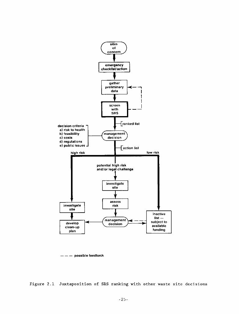
Figure 2.1 shows the suggested relationship of the SRS ranking to the overall program to reduce hazards at waste sites. are described below.
The headings of Figure 2.1
Emergency checklist/action. After discovery, a site evaluation begins by quickly evaluting the acute hazards ( B . Murphy, prsnl. comm., 1987) . If acute hazards are present and no barriers protect the public, then immediate action must be taken. An emergency checklist might include the following questions and suggested emergency action:
Can the public directly contact any hazardous materials (especially acutely hazardous materials)? Control access to the site.
Is drinking water contaminated at the tap? Find an alternate drinking water source.
Is there a serious threat from flammable or explosive materials? Neutralize or remove the material.
Are acutely hazardous materials stored in weak bulk containers or present at or very near the soil surface or can wind or water easily disperse the material? Remove or thoroughly cover and protect the material.
SRS screening. The second major step of a site evaluation involves Ranking the sites of concern is an integral part of the scoring with SRS.
overall assessment and management of risk; thus, the basis of the ranking scheme must be similar to risk assessment methodology to ensure a consistent ranking. we developed SRS.
Because currently existing ranking schemes did not have this basis,
Because SRS is risk based, the information gleaned from the ranking can guide further data collection efforts; hence some interaction may occur between screening and collection of readily available data (Figure 2.1).
- 2 4 -
I -
-
.-
emergency checklist/action
gather preliminary - 1
I I I I screen
with --
decision criteria - a) risk to health b) feasibility
d) regulations e) public issues - c) costs
action list gh risk low ri!
potential high risk and/or legal challenge
I
investigate
inactive
subject to available funding
develop decision clean-up
--- possible feedback
Figure 2.1 Juxtaposition of SRS ranking with other waste site decisions
- 2 5 -
Management decision. Considerations such as ecologic hazards, cost to clean up a site, technical feasibility, public concerns, or risk-management
policies of a regulatory agency have been omitted in SRS; consequently, the ranked list is not necessarily a final action list; the ranked list provides only technical input on human health risk. The final action list is a result of risk management decisions (Risk Assessment, 1983) based on the technical input of SRS and these other factors.
Many ranking schemes combine aspects of both risk assessment and risk management. There are instances when the risk management decision criteria are rigid enough to incorporate into a ranking scheme, but in general the decision criteria are not and, thus, this practice is not recommended (Risk Assessment, 1983). Combining risk assessment and risk management can frequently confuse industry and the public over decisions based on the ranking scheme. It also reduces the portability between governmental agencies with different decision criteria. Furthermore, it also reduces the flexibility of the risk manager to manage. For example, some sites are easier to clean up; thus, a grouping (portfolio) that includes easily cleaned up sites, not necessarily the worst sites, may reduce overall health risks more for the money spent.
Site KrouDings. Following the management decision step, sites will be set into three groups: high risk, potentially high, and low risk sites. The high risk sites will undergo detailed RI/FSstudies, highest SRS scores first, and then cleanup. The potentially high risk sites will undergo detailed site
investigations (highest SRS scores first), detailed risk assessment, and then through another risk management decision step. Nothing more will be done for sites in the low risk group unless additional cleanup fundings are available. The number of sites in each group will depend upon management decisions. An agency may decide to group most sites into the high or low risk groups, requiring only a few undergo a detailed risk assessment. Alternatively, an agency may require most sites undergo a detailed risk assessment while only a few are automatically set in the high and low risk groups.
Before summarizing conclusions from Chu et al. concerning existing ranking methods, we present a very brief description of SNTA's proposed risk
- 2 6 -
methodology as background to help explain what "detailed risk assessment" entails.
SNLA Proposed Risk Methodologv
To perform probabilistic risk assessments, one must evaluate both the probabilities and consequences of events that could lead to release of contaminants from a waste site and then transport to a specific target of concern. The five steps in the assessment usually are
disposal system characterization (waste properties, site characteristics, and facility design);
scenario development, probability estimates, and screening;
9 consequence modeling;
risk calculations and/or comparison with government regulations; and
sensitivity/uncertainty analysis.
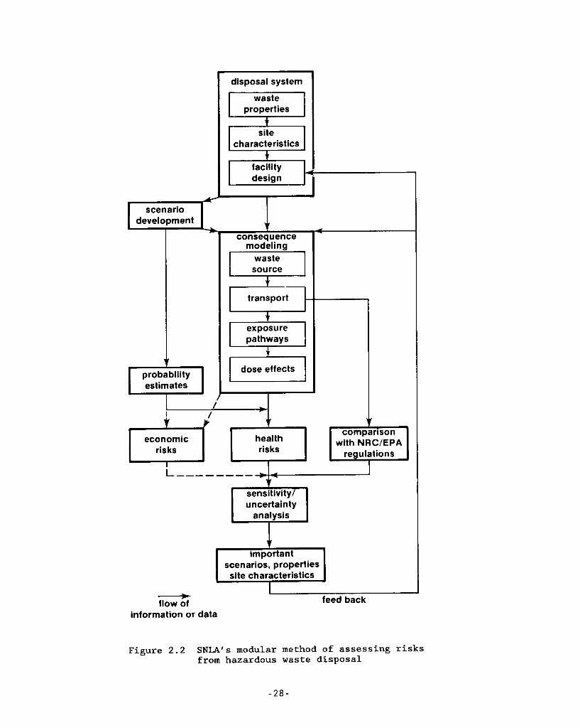
SNLA's modular approach to risk assessment, based on extensive experience for high-level radioactive waste repositories (Cranwell et al., 1987), is shown in Figure 2.2. The five components of the methodology are represented by the various modular blocks. advantages for the analyst:
This modular approach has several
The analyst, by examining intermediate results, gains insight into physical processes and important parameters affecting risk.
The analyst can use intermediate results directly in determining compliance with regulatory standards (for example, 40CFR264)
The analyst can more easily modify the methodology, if necessary.
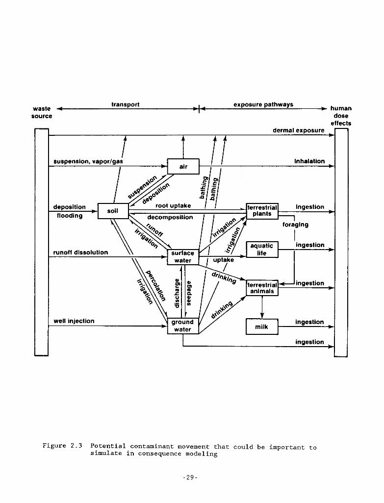
Because a large portion of the methodology consists of simulating physical processes to estimate consequences from waste release (consequence modeling), Figure 2.3 illustrates a classical, detailed breakdown of the numerous pathways that would have to be examined,
Even if all the necessary data were available, analyzing every intricate pathway would be time consuming. Hence, in addition to consequence modeling, an important part of a risk assessment is sensitivity and uncertainty
disposal system
scenario development
waste
site
facility
estimates
economic
A consequence
modeling
source
I transport 1 F5 exposure
pathways 2 I dose effects I
health risks
with NRC/EPA
I
uncertainty analysis
scenarios, properties
I site characteristics , -
flow of information or data
feed back
Figure 2 . 2 SNLA's modular method of assessing r i sks from hazardous waste disposal
- 2 8 -
-
transport exposure pathways waste 4 + human source dose
effects dermal exposure
well injection water
L ingestion
Figure 2.3 Potential contaminant movement that could be important to simulate in consequence modeling
- 2 9 -
analysis (Figure 2.2). Sensitivity analysis identifies those parameters that most influence the total risk. Uncertainty analysis identifies uncertainty in the results because of uncertainty in models and input parameters.
Obviously from Figures 2.2 and 2.3, a detailed assessment of health risk at a site is time consuming and expensive. Consequently, sites of concern must be ranked to identify sites that are more likely sources of contamination and, thus, hazards to the public. Before developing SRS, we reviewed the current ranking methods available.
Review of Rankinv Methods
Chu et al. (1986) reviewed ranking and screening procedures created for a variety of purposes. Although most were only marginally relevant for DOE, three of the procedures surveyed were examined in detail. These were the Hazard Ranking System (HRS), developed by MITRE Corporation for EPA (HRS Workshop, 1982); the modified Hazard Ranking System (mHRS), a modification of
HRS by Battelle Pacific Northwest Laboratory (PNL) to include radioactive wastes (Hawley and Napier, 1985); and the Hazard Assessment Rating Methodology (HARM), created by the U.S. Air Force for its installation restoration program (USAF, 1983). A fourth detailed ranking scheme under development, RAPS (Whelan et al., 1986), is also discussed. Because of drawbacks in the currently available schemes (HRS, mHRS, and HARM) and because they lacked a risk basis, SNLA strongly recommended developing a new site ranking system (SRS) for DOE hazardous waste sites.
Hazard Ranking System (HRS). HRS, requiring limited data, is simple to use. By virtue of its use in selecting almost 900 hazardous sites for listing on the National Priorities List (NPL) (40CFR300), HRS is the standard method for ranking hazardous waste sites.
Although it does not quantify the probability or magnitude of harm that could result from a waste site, HRS ranks sites by scoring factors that influence these elements of risk. HRS scores
- 3 0 -
I-
......"
.I.
the manner in which hazardous wastes are contained,
the pathway by which they could be released,
the characteristics and total amount of harmful substances,
the likely targets (receptors) harmed.
Specifically, HRS assigns three scores to a hazardous waste site:
The migration score [F ] indexes the potential harm to humans or sensitive environmentsMbecause of the waste migrating away from the site along a ground-water, surface-water, or air pathway. geometric average of separate scores for each of these three pathways.
FM is the
The flammable and explosive score [F 3 indexes the potential harm FE from flammable or explosive material.
The direct-contact score [FDC] indexes the potential harm from direct exposure (no migration) to a human intruding into the site.
EPA usually uses FFE and FDC to identify sites requiring emergency
M attention; thus, the migration score F is the primary score for ranking. Three major factors comprise the migration score [FM]: waste, pathway, and target characteristics. The pathway factor is given the maximum score if any release of a hazardous substance has occurred. EPA ranks and places sites on the NPL if the final score is above 28.5 (HRS Workshop, 1982) .
HRS has several strengths (HRS Workshop, 1982) : e
It is simple to use. Once the value of a parameter is known, one looks up its score in a table.
It does not require extensive data.
The parameters selected affect risk and are not redundant.
It gives a wide range of scores.
The three major migration pathways are considered, and the geometric averaging of the individual pathway scores does not severely dilute one important pathway when the other two are unimportant.
Yet, HRS has drawbacks. First, HRS ignores several properties of the hazardous wastes that directly influence the human health hazard. Although HRS scores waste properties (persistence, toxicity, and quantity), the manner in which they are scored distorts the results:
- 3 1 -
The score for toxicity is based on only the most hazardous substance, rather than a composite of the entire waste inventory. In contrast, total mass of glJ substances is used to quantify the magnitude of this hazard--quantity is not linked to each (or a category of) chemical.
Only the severity of effect (regardless of required dose) is considered when rating the chemical toxicity using SAX scores (Sax, 1975); consequently, radionuclides, which may cause cancer, automatically receive the highest toxicity score regardless of dose
Only the initial quantity of waste is considered, even though similar quantities over markedly different areas pose different threats.
Second, problems exist with scoring the population:
HRS does not address the elapsed time before exposure.
Distance is used as a weighting factor in situations where release has already occurred. where the release is observed.
This may or may not be appropriate, depending on
Third, HRS ignores several important characteristics of the pathway:
HRS does not account for the direction of the hydraulic gradient.
HRS does not score the air pathway unless release has been observed.
HRS uses an arbitrary 3-mile radius for the ground-water pathway regardless of the hydrogeologic conditions.
Sorption properties of the soil are not considered in the ground-water or surface-water pathways.
HRS gives no guidance on what monitoring data are acceptable and what defines a "significant" release--important because observed releases overwhelm the HRS score, especially for the air pathway.
Finally, several general criticisms of HRS have also been raised:
HRS, being highly subjective, sometimes has problems in ranking sites because the score can be manipulated too easily by the analyst, especially by choosing whether or not to collect data for "evidence of contamination. 'I
HRS sometimes adds scores, sometimes multiplies them, and finally finds the geometric average of the scores for the different pathways (air, surface water, and ground water)--combining rules that have little connection with the comprehensive tools and procedures of risk assessment.
Sites posing only risks to sensitive environments usually rank low; HRS heavily weighs sites posing human health risks.
- 3 2 -
Hazards from food chains are not considered.
HRS combines both risk assessment and risk management decisions.
The new authorization of Superfund that passed in October 1986 [Superfund Amendments and Reauthorization Act (SARA, 1986)] requires EPA to correct and/or comment on many of these specific problems in HRS within 2 years. Because the logic for HRS was not readily apparent, we could not confidently understand the implication of any changes we made ourselves. Thus, we chose to develop an entirely new ranking system.
Modified Hazard Ranking Svstem (mHRS). Battelle Pacific Northwest Laboratories (PNL) (Hawley and Napier, 1985) modified HRS for the DOE Office of Operations Safety to rank sites that contained both chemical and radioactive hazardous wastes (that is, mixed-waste sites), as occurs at DOE facilities. wastes and had a severe, albeit possibly unintentional, bias against them. Yet, EPA required DOE to rank their current and abandoned waste sites for possible listing on the NPL. The mHRS is identical to HRS except that mHRS splits the waste characteristics scoring into two parts--one for chemical wastes and one for radioactive wastes. The highest score from the two parts is used in further calculations for scoring the site. Although alleviating a limitation, mHRS still suffers from the other drawbacks of HRS.
This was necessary because HRS was not developed for radioactive
Hazard Assessment RatinP Methodology (HARM). The Department of Defense (DOD) has established a program to identify and control problems at its hazardous waste sites to comply with the intent of RCRA (1976), similar to the purpose of the DOE HAZWRAP program. The U.S. Air Force uses HARM for ranking sites under its control. It is a highly modified version of the ranking model developed for EPA by JRB Associates (Kufs et al., 1980). Because the JRB model was also the starting point for HRS, it is somewhat similar. quantity--a more realistic approach. However, HARM inappropriately scores persistence by using the most persistent chemical in the waste inventory.
HARM scores hazards of the waste by considering both toxicity and
Remedial Action Priority Svstem (RAPS). PNL has been developing since FY 1983 a computer-based ranking system called RAPS for the Office of Environmental Guidance and Compliance, also at DOE (Whelan et al., 1986).
- 3 3 -
Like SRS, RAPS is based on risk methodology; hence, they can work together in tandem--SRS for screening and RAPS for more detailed risk assessment.
Using empirical, analytic, and semianalytic algorithms, RAPS addresses many limitations of HRS. It considers
more site and waste characteristics,
both chemical and radioactive wastes,
waste dispersion and decay,
individual chemical toxicity
population distributions,
three exposure routes: external, inhalation, ingestion,
duration of exposure,
time until population exposed.
RAPS outputs a hazard potential index (HPI) (not an absolute but a relative measure of risk) that can be used to rank the site relative to other sites. To obtain the HPI, RAPS considers four major pathways: ground water, overland, surface water, and air.
RAPS is not entirely operational. Currently, PNL is working on a version of RAPS for the personal computer. A preliminary PC version should be completed by September 1987. The entire RAPS system should be ready by September 1988 (G. Whelan, persl. comm., 1986).
Ranking system modifications. During the development of SRS, the previously discussed ranking systems were undergoing modifications (sometimes extensive) (B. Madison, EPA, prsnl. comm., 1987): the State of New York developed the New York System from HRS; ORNL developed the Defensive Prioritization System (DPM) for the U.S. Air Force by extensively modifying HARM; and EPA began revamping HRS. Perhaps all the ranking scheme will converge toward the same philosophy, but reports are currently unavailable; thus, we have not evaluated their theory or improvements.
- 34-
I-
--
Incidents from Waste Disposal Sites
As background information for the reader, we present data on incidents
of contamination from the 1970s that influenced the development of SRS. A frequently cited paper, Lazar et al. (1976), describes and tabulates 421 incidents of damage from land disposal of industrial hazardous wastes (Table 2.1). The hazardous wastes harm humans or biologic systems by five general mechanisms (in order of importance):
contaminating ground water, contaminating surface water, being accessible to direct human contact, contaminating the air around the site. causing a fire and/or explosion
Of the five mechanisms, exposure to the waste via ground water is the most prevalent (roughly 60% of cases in the EPA survey); hence, a ranking system should be strongest in evaluating the potential human risk via this pathway. Paradoxically, information on the ground-water pathway is frequently unknown, perhaps because it is simply not visible and thus expensive to discern.
The most frequent contamination of surface water resulted from haphazard disposal on vacant property (41%). (In addition, Table 2.1 shows that most incidents of direct contact poisoning came from haphazard disposal.) Surface- water contamination from landfills and lagoons accounted for 29 and 25% of the incidents, respectively. RCRA (1976) and supporting EPA regulations (40CFR264) have attempted to reduce surface-water Contamination significantly at engineered sites by requiring hydraulic structures to prevent storm flow onto and off the waste sites. The interim regulations for active sites require structures capable of handling storms of 24-hr duration and a return period of 25 yr or less (40CFR264). means that, on average, an event of this magnitude, or greater, is not expected to occur more often than once in 25 yr.)
(A storm with a return period of 25 yr
The air pathway was significant in only 4% of the contamination cases reported in the preliminary study, implying that the air pathway will
- 3 5 -
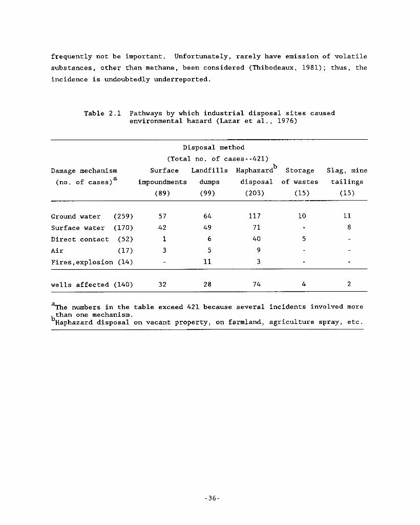
frequently not be important. Unfortunately, rarely have emission of volatile substances, other than methane, been considered (Thibodeaux, 1981); thus, the incidence is undoubtedly underreported.
Table 2.1 Pathways by which industrial disposal sites caused environmental hazard (Lazar et al., 1976)
Disposal method (Total no. of cases--421)
Damage mechanism Surface Landfills Haphazardb Storage Slag, mine (no. of cases) impoundments dumps disposal of wastes tailings a
(89) (99) (203 1 (15) (15)
Ground water (259) 57 64 117 10 11
Direct contact (52) 1 6 40 5 Air (17) 3 5 9 Fires,explosion (14) - 11 3 -
Surface water (170) 42 49 71 8
wells affected (140) 32 28 74 4 2
a The numbers in the table exceed 421 because several incidents involved more than one mechanism.
bHaphazard disposal on vacant property, on farmland, agriculture spray, etc.
- 3 6 -
3. GENERAL ASPECTS OF SRS
This chapter discusses the basis and general framework of SRS. The next
four chapters ( 4 , 5 , 6 , and 7) describe in more detail the factors selected for scoring.
Overview of SRS
Before delving into the justification of the scoring concept of SRS, we briefly present (1) the simplified pathways used and the overall scoring procedure, and (2) the principles that guided the development of SRS.
--
A
The complex movement of contaminants in the environment depicted in Figure 2.3 is greatly simplified for SRS. Intricate exposure pathways involving food chains are not considered. Instead, the exposure route involves only direct ingestion of surface or ground water or inhalation of air. Furthermore, recycling of contaminant between surface water, ground water, surface soil, and air is assumed to comprise a minor component of health risk. Figure 3.1 shows these and several other simplifying assumptions used for modeling the consequences of contaminant release from a site.
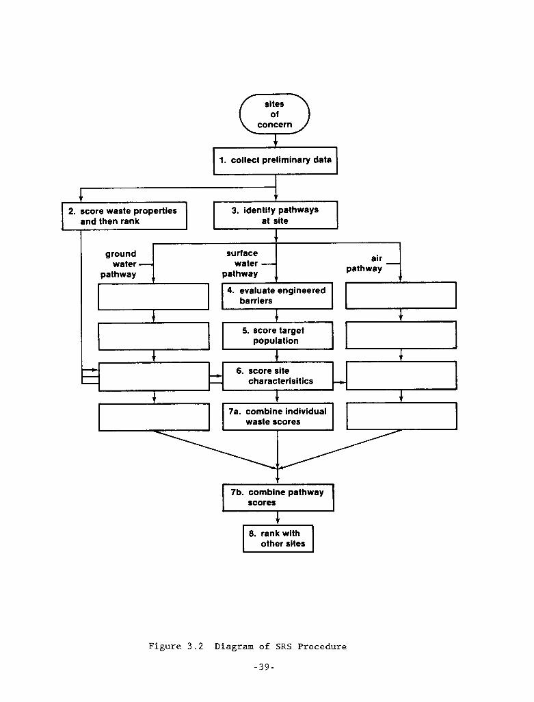
The ranking technique involves (Figure 3.2)
collecting data on waste properties, site characteristics, and facility design;
ranking the wastes found at the site by quantity and toxicity to screen out relatively minor waste components;
describing the release pathways of concern for the site;
evaluating engineered features at the facility;
identifying target populations along these pathways;
scoring site characteristics based on the manner waste escapes from the site (ground-water, surface-water, and air pathways);
combining individual waste scores to arrive first at a pathway score and finally at a site score;
ranking the site in relation to other scored sites.
-37-
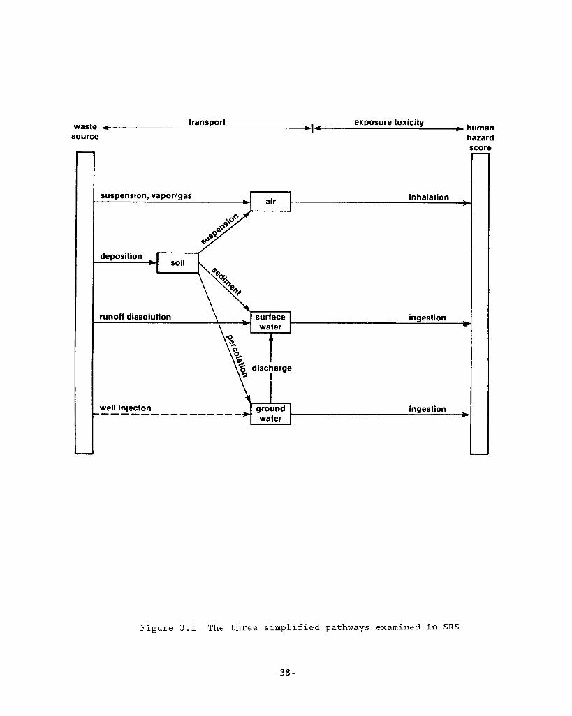
transport exposure toxicity waste 4 b human source hazard
score
suspension, vapor/gas inhalation
ingestion
well injecton ingestion .---- -----------
Figure 3.1 The three simplified pathways examined in SRS
- 3 8 -
--
_I^
-
_-
+ -
6. score site - - - characterisitics +
? 1. collect preliminary data
I
and then rank at site
7a. combine individual waste scores
ground water
surface water
rathway 1 , ;ath;Waiers+ , 4. evaluate engineered
5. score target ---
Figure 3 . 2 Diagram of SRS Procedure
- 3 9 -
PrinciDles Guiding: DeveloDment of SRS
Although listing factors that could influence the ranking of a hazardous waste site is easy, developing a credible, scientifically defensible, ranking methodology is difficult. Furthermore for the ranking scheme to be useful in the risk evaluation proposed by SNLA (Figure 2.1), the choice of parameters, scales for scores, and rules for combining scores must be consistent with the detailed risk assessment methodology. systems (Chu et al., 1986) concluded that, although plausible, they failed tests for consistency.
Our review of completed ranking
Several principles and goals guided our development of SRS: SRS was to
approximate the ranking obtained with a detailed risk assessment, and thereby, improve upon H R S ;
have a logic easy to understand and use;
work with preliminary site data;
require only data that have an order-of-magnitude effect on the health risk, to be consistent with the uncertainty of preliminary data;
be applicable to most waste sites.
These principles and the reasons for incorporating them into SRS are discussed in the next few paragraphs.
Risk assessment basis. The basis of SRS is risk assessment methodology. Specifically, in the SRS scoring system, the score is an approximation of a risk assessment calculation. This rationale was used to ensure that the number of false positives (innocuous sites ranked among those felt to be dangerous) and false negatives (dangerous sites ranked among those felt to be innocuous) would be small. In addition, with this approach the parameters and the manner in which they contribute to the risk can be easily identified. For example, if two factors such as exposure and toxicity combine multiplicatively in the risk assessment, then they combine multiplicatively in the ranking scheme also. A scoring system thus derived likely includes the most important parameters and combines them in a consistent manner, so
that distortions are minimized. We have attempted to ensure this consistency in SRS. Indeed, it is an advantage over many other ranking schemes.
-40-
1-1
Of course, if we could devise a scoring system that accurately mimicked a detailed risk assessment, an analyst would not need the latter. Numerous compromises are necessary. shortcoming; a simpler and less mathematically rigorous system can be easier to use with preliminary site data that may at times be only descriptive.
But these simplifications are not always a
ImDrovement over HRS. By basing SRS on risk methodology, we readily were able to understand how to improve upon H R S . In contrast to H R S , SRS
uses a more accurate measure of toxicity;
handles both chemical and radioactive hazardous wastes;
evaluates the health hazard from the quantity of each constituent comprising the waste;
more adequately evaluates the risk from surface-water runoff;
considers ground-water flow direction and distance;
evaluates the potential hazard from the air pathway even without observed releases;
does not use arbitrary maximum distances to targets of concern;
accounts for environmental attenuation of the hazardous material;
separates risk assessment from risk management decisions.
Several of these improvements were required by SARA (1986), others are improvements under consideration by EPA (Caldwell, 1986).
Understandable logic. Although using a risk assessment approach, SRS is easily understood and simple to score. Ease of use is important because SRS is a preliminary screening tool, not a replacement for detailed risk assessment or field monitoring. A clear logic is important because it helps ensure the successful application and versatility of the ranking procedure.
Use with readilv available data. The ease with which scores are assigned is influenced by the data required. For example, even complex computer systems can be easy to use, but the amount of data required may, in turn, require massive amounts of time and money to collect. We assumed the most difficult and expensive part of ranking a waste site was collecting
-41-
data, especially for the many abandoned sites that have little information available. Compared to scoring systems such as HRS, the major change in required data concerned collecting more detailed information on type, properties, and amount of hazardous waste stored.
Data uncertaintv. Preliminary data gathered at a site is likely to have large uncertainty. For example, the identity and amount of hazardous material disposed of at an abandoned site is often unknown. even though a complex model might exist for ground-water transport of a material, the added precision contributed by this model does not improve the certainty of the prediction because the source term is so uncertain; the added data requirements for the precise model are not justified. Therefore, we only used models (and thereby factors) that had a major effect on the result. In summary, our premise was that when large data uncertainty exists, a simple model involving the major processes is as adequate as a complex one and, thus, does not hamper predictions.
Accordingly,
General aDulicabilitv. Finally, although SRS was specifically developed for DOE, we kept it general such that one could apply it, possibly with minor modifications, to the whole spectrum of land-based waste sites currently existing [for example, chemical or sanitary landfills and lagoons, leaking surface or underground storage tanks, mill tailings and other waste piles, injection wells, accidental spills, and roadside (or vacant land) contamination from illegal dumping]. future disposal sites; however, we strongly caution that bounding calculations from simple analytical models (as used in SRS) can possibly eliminate many good sites.
SRS may even be useful for selecting
Scorinv ConceDt of SRS
Because SRS is risk-based, an important starting point is the measure of A
risk. risk to other ecosystems [Re], and risk to economic institutions [R 1 . principle, all could be included to obtain total risk [R]. Normally, however, subjective weights [ y , cp] would be assigned to the ecosystem and economic risk components (Symbol definitions are repeated in Appendix E):
Several measures of risk are possible: risk to human health [ % I , A A
In A $
- 4 2 -

--
I
A
SRS uses only human health risks [%I; other risks are described but not scored. The latter risks can be brought into the decision process when the risk manager is selecting the priority sites.
A
Risk [%] is the product of the probability [PI of a scenario and the consequence [$,I of that scenario. Here, a scenario is a sequence of events that could lead to release and transport of hazardous chemicals from a waste site to some target (receptor) that could be endangered. Usually, a large number of scenarios can be developed; health risk is the sum of these individual risks:
h
% = c Pi$i i = 1, number of scenarios
The risk can be subdivided into chronic risks, which occur over long periods of time, and acute risks, which occur suddenly. Chronic risks are approximated by annualized health effects at steady-state conditions. Acute risks are irregular occurrences associated with brief increases in risk. According to the public's disposition toward risk aversion, a risk modeler may need to subjectively weigh (7) acute risk more:
h
% = c Pidi
SRS considers only the potential risk to humans [%I from chronic scenarios. Acute risks from fire, explosion, or direct contact are noted in the narrative accompanying the ranking. rapid response (for example, separating certain chemicals or building a security fence around the site) as opposed to long-term remedial response (for example, stabilizing lagoon wastes) as scored in SRS.
+ c -y.P.lc, i = chronic scenarios, j = acute scenarios J J j
A
These types of problems require
In SRS, risk is measured by summing consequences [$] from three generic pathways. The generic pathways are identified by the manner in which hazardous waste leaves the site: either through an air, surface-water, or ground-water route. For initially screening waste sites, it is impractical to develop numerous mutually exclusive scenarios and estimate their probabilities of occurrence. Hence, the complicated contaminant pathways
I - 4 3 -
depicted in Figure 2.3 are replaced with three greatly simplified pathways (Figure 3.1). These three generic migration pathways comprise the release scenario, which has a probability of one of occuring. (Release is not necessarily simultaneous or equal along all pathways.)
k - number of pathways; P = 1 ;k-c$k k l3.11
SRS assumes that the consequence ($1 (for example, chronic illness or cancer death) of any pathway is influenced by three factors: the size of the population at risk [N], the exposure [E] of that population to the hazardous material, and the toxicity of hazardous material [TI. Let toxicity be expressed as age-adjusted annual risk per rate of exposure, assuming an average 70-yr life [for example, (1/70) (lifetime risk per mg/kg/day)]. Further, assume that the risk to an average population, not a sensitive subset such as children, is the ranking index of interest. Finally, let exposure be expressed as a daily rate (for example, mg/kg/day). Then the annual number of instances of chronic illness or cancer deaths, which is the consequence [$I, is
Furthermore, the consequence [$I of any pathway for all chemicals is the sum of the consequences from each hazardous chemical or radionuclide of the inventory at the waste site; hence, the risk is proportional to
A
R = chemical, k = pathway Rh a E NRk' TRk
Of these three factors, two--population and toxicity--are easily characterized by single "scores" in a ranking system and discussed in Chapter 4. Only exposure [E] must be disaggregated further into component factors.
The specific component factors of E, which vary with each pathway, are discussed in detail in Chapters 5, 6 , and 7, but generally the amount of exposure is evaluated from the quantity of material initially deposited at the site [Wo] and the factors indexing the effectiveness of the engineered barrier [f ] (for instance, waste package or facility design) and site
eng
- 4 4 -
features [fsite] in reducing the amount of hazardous substance reaching the potentially exposed population:
E a W o o f eng fsite i3.41
Substituting equation [3.4] into [3.3] yields (assuming the population [N] does not change with the chemical)
1 - chemical, k - pathway [3.5] 4 a E Nk a TQk [ '0 feng fsite 1 Rk In a detailed risk assessment, the mass of waste [Wo] should be divided among the various pathways; however, SRS only roughly estimates the health risk, thus, this minor adjustment in equation [3.5] is unnecessary. The abstractness of equation [3.5] belies the relative simplicity of SRS revealed in Figure 3.2.
Scoring Individual Factors
We made SRS easier for hand calculations by tabulating "scores" for the individual factors as done with most hand ranking systems. We selected the appropriate scores by simply using the logarithms of the factors in the basic ranking equation [3.2]. These individual scores can then be added (subtracted) rather than multiplied (divided) to arrive at the overall score. For example, the logarithm of the expression for exposure, equation [3.4] is as follows:
log (E) a log Wo + l o g f + log fsite l3.61 eng
Furthermore, because the various site parameters that influence E will likely be known within only a factor of ten, using preliminary data, we used only the logarithm to the nearest integer (the characteristic).
To substitute equation [3.6] into [3.5], one must first take the antilogarithm. Yet, the score has already been based on the assumption that the preliminary data are not better than a factor of 10; thus, we can approximate the addition by taking the largest of the logarithm scores. For
-45-
instance, a score of 1 for one chemical along a pathway added to a score of 3 for another chemical results in a pathway score of 3 (10 1 3 + lo3 = 10 ) .
However, if several chemicals have the same large score, the score should be increased. A simple rule such as
Ft = F
F t Fa
+ 0.1 n a a + 0.01 rj, + . . . where
= total score; e.g., Ft = log (C ERTn) = highest individual score; e.g., F = log E T a R R
n = number of chemicals with score F
n,,
a a b = number of chemicals with score one unit less F
Fb = next highest individual score
suffices for hand calculations. For instance, suppose 10 chemicals all had a score of 8 . Using equation [3.7] we would assign a score of 9, which on a logarithm scale is 10 times as bad as a score of 8 . To be consistent with data inaccuracies, one should round equation [ 3 . 7 ] . For example, if more than 3 chemicals have the same score, increase it by a full unit.
There are several advantages to selecting the logarithm, rounded to the nearest integer, as the score for SRS:
It simplifies the hand calculations; only order-of-magnitude effects are scored.
It automatically restricts the sensitivity of the ranking system to order-of-magnitude effects.
It makes SRS similar to other ranking systems, yet selection of scores is easily understood if modifications are necessary; furthermore, the scores are not excessively large or small.
We must acknowledge a disadvantage, best demonstrated with an example, that often exists with other hand ranking systems as well. If SRS scores two different sites as 20 and 25, then SRS has measured a five order-of-magnitude difference between them; however, this difference is not readily conveyed to an analyst with only a 5-point spread in the scores. We feel the advantages outweigh this disadvantage; however, the analyst is by no means restricted to the logarithmic scoring system. The analyst can record the actual numerical
- 4 6 -

value of each factor on the worksheets and multiply, divide, add, and subtract as required by the models on which SRS is based.
Programming the basic SRS equation (equation [ 3 . 7 ] along with the expressions for exposure discussed in Chapters 5, 6 , and 7) on a personal computer could eliminate the need for logarithmic approximations. Indeed, we plan to do this; however, we also wanted SRS to be workable with hand calculations to maintain its versatility while developing and checking its feasibility.
Sensitivityflncertainty Analysis
SRS was developed to effectively allocate resources towards those sites with the greatest potential risk. However, SRS is most necessary when little information on sites is available; therefore, a risk manager also must know the important data to collect based on the potential impact of that data. This knowledge in turn, requires understanding the ranking system.
The SRS model equations developed in Chapters 5, 6 , and 7 list the variables to measure or index to evaluate consequences of hazardous waste release along the three pathways (for example, fluid pore velocity [V ] and waste quantity [W 3). Yet, we can glean more understanding from these equations through sensitivity/uncertainty techniques (Iman et al., 1981a, 1981b).
gw 0
A detailed sensitivity/uncertainty analysis was not within the scope of the first phase of developing SRS. Hence, we do not present results from a detailed analysis but rather describe here the added insight the analysis provides and how we incorporated the concepts into SRS.
General definitions. With sensitivity/uncertainty analysis we evaluate the potential variation of variables and their relative importance on the results.
A 1’ * * variables X l,...,\. Because X R(X1, . . . , Xk) will also have a range and distribution. Uncertainty analysis involves determining properties of the distribution of R. These properties include the distribution, expected value, and variance of R. Sensitivity
A
Specifically, the SRS ranking model is a function R(X 1’ * * .\> of . , \ have ranges and distributions,
A
A
- 4 7 - -
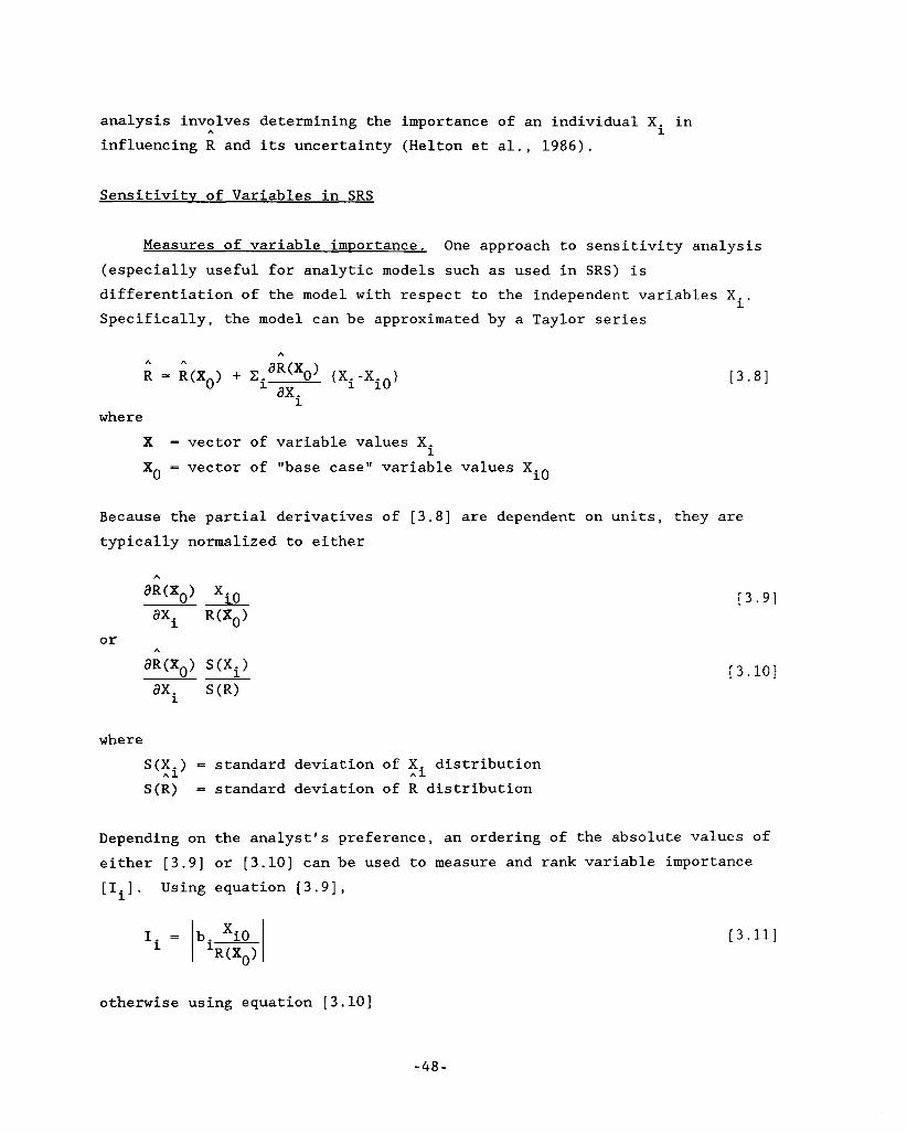
analysis involves determining the importance of an individual X in influencing R and its uncertainty (Helton et al., 1986).
A i
Sensitivity of Variables in SRS
Measures of variable imDortance. One approach to sensitivity analysis (especially useful for analytic models such as used in SRS) is differentiation of the model with respect to the independent variables Xi. Specifically, the model can be approximated by a Taylor series
A A A
R = R(XO) + Ci aR(XO) (Xi -xio 1 axi ~3.81
where X = vector of variable values X X
i = vector of "base case" variable values Xio 0
Because the partial derivatives of [3.8] are dependent on units, they are typically normalized to either
or A
13.91
[3.10]
where S(X.) = standard deviation of X. distribution S(R) = standard deviation of R distribution
A 1 A 1
Depending on the analyst's preference, an ordering of the absolute values of
either [3.9] or [3.10] can be used to measure and rank variable importance [Ii]. Using equation [3.9],
[3.11]
otherwise using equation [3.10]
-48 -
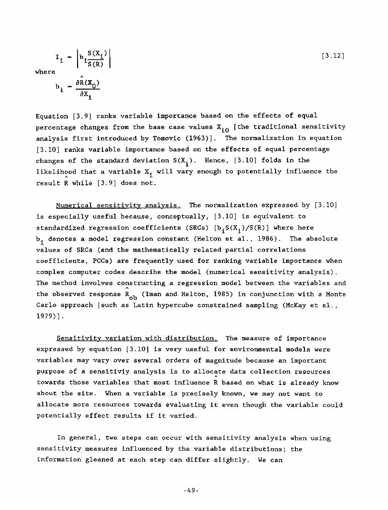
where A
aR(xo> axi bi -
[3.12]
Equation [3.9] ranks variable importance based on the effects of equal percentage changes from the base case values Xio [the traditional sensitivity analysis first introduced by Tomovic (1963)l. The normalization in equation [3.10] ranks variable importance based on the effects of equal percentage changes of the standard deviation S(Xi). likelihood that a variable Xi will vary enough to potentially influence the result R while [3.9] does not.
Hence, [3.10] folds in the
A
Numerical sensitivitv analysis. The normalization expressed by [3.10] is especially useful because, conceptually, [3.10] is equivalent to standardized regression coefficients (SRCs) [biS(Xi)/S(R)] where here b denotes a model regression constant (Helton et al., 1986). The absolute values of SRCs (and the mathematically related partial correlations coefficients, PCCs) are frequently used for ranking variable importance when complex computer codes describe the model (numerical sensitivity analysis). The method involves constructing a regression model between the variables and the observed response R (Iman and Helton, 1985) in conjunction with a Monte Carlo approach [such as Latin hypercube constrained sampling (McKay et al., 1979) ] .
A
i
A
ob
Sensitivitv variation with distribution. The measure of importance expressed by equation [3.10] is very useful for environmental models were variables may vary over several orders of magnitude because an important purpose of a sensitiviy analysis is to allocate data collection resources towards those variables that most influence R based on what is already know about the site. allocate more resources towards evaluating it even though the variable could potentially effect results if it varied.
A
When a variable is precisely known, we may not want to
In general, two steps can occur with sensitivity analysis when using sensitivity measures influenced by the variable distributions; the information gleaned at each step can differ slightly. We can
-49-
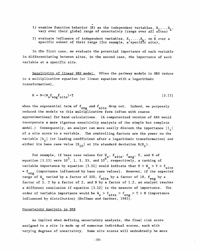
A
1) examine function behavior (R) as the independent variables, XI,. . *%, vary over their global range of uncertainty (range over all sites)
A
2) evaluate influence of independent variables, X1, ...,%, on R over a specific subset of their range (for example, a specific site),
In the first case, we evaluate the potential importance of each variable in differentiating between sites, in the second case, the importance of each variable at a specific site.
Sensitivity of linear SRS model. Often the pathway models in SRS reduce to a multiplicative equation (or linear equation with a logarithmic transformation),
R = N*(W f f )*T o eng site [3.13]
drop out. Indeed, we purposely and fsite when the exponential term of f reduced the models to this multiplicative form (often with coarse approximations) for hand calculations. (A computerized version of SRS would incorporate a more rigorous sensitivity analysis of the simple but complete model.) Consequently, an analyst can more easily discern the importance [ I . ]
of a site score to a variable. The controlling factors are the power on the variable [b.] (or leading coefficient after a logarithmic transformation) and either its base case value [X ] or its standard deviation S ( X . ) .
eng
1
1
io 1
For example, if base case values for W T, and N of 3 40* fsite’ feng’ equation [ 3 . 1 3 ] were 10 , 1, 1, 15, and 10 , respectively, a ranking of variable importance by equation [3.11] would indicate that N > W > T > fsite = f (importance influenced by base case values). However, if the expected
range of Wo varied by a factor of 100, fsite by a factor of 10, f by a factor of 5, T by a factor of 2, and N by a factor of 1.2, an analyst reaches a different conclusion if equation [3.12] is the measure of importance. The order of variable importance would be W influenced by distribution) (Hoffman and Gardner, 1983).
0
eng eng
> fsite > f 0 eng > T > N (importance
Uncertaintv Analysis in SRS
As implied when defining uncertainty analysis, the final risk score assigned to a site is made up of numerous individual scores, each with varying degrees of uncertainty. Some site scores will undoubtedly be more
- 5 0 -
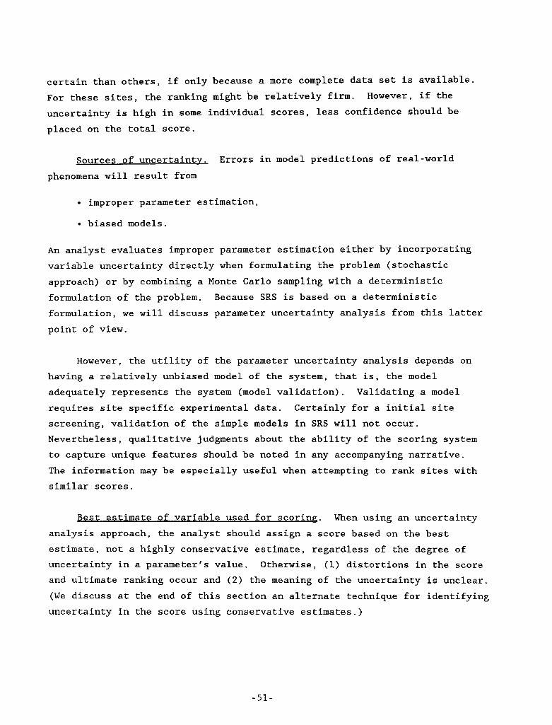
certain than others, if only because a more complete data set is available. For these sites, the ranking might be relatively firm. However, if the uncertainty is high in some individual scores, less confidence should be
placed on the total score.
Sources of uncertaintv. Errors in model predictions of real-world phenomena will result from
improper parameter estimation,
biased models.
An analyst evaluates improper parameter estimation either by incorporating variable uncertainty directly when formulating the problem (stochastic
approach) or by combining a Monte Carlo sampling with a deterministic formulation of the problem. Because SRS is based on a deterministic formulation, we will discuss parameter uncertainty analysis from this latter point of view.
However, the utility of the parameter uncertainty analysis depends on having a relatively unbiased model of the system, that is, the model adequately represents the system (model validation). Validating a model requires site specific experimental data. Certainly for a initial site screening, validation of the simple models in SRS will not occur. Nevertheless, qualitative judgments about the ability of the scoring system to capture unique features should be noted in any accompanying narrative. The information may be especially useful when attempting to rank sites with similar scores.
Best estimate of variable used for scoring. When using an uncertainty analysis approach, the analyst should assign a score based on the best estimate, not a highly conservative estimate, regardless of the degree of uncertainty in a parameter's value. Otherwise, (1) distortions in the score and ultimate ranking occur and (2) the meaning of the uncertainty is unclear. (We discuss at the end of this section an alternate technique for identifying uncertainty in the score using conservative estimates.)
- -51-
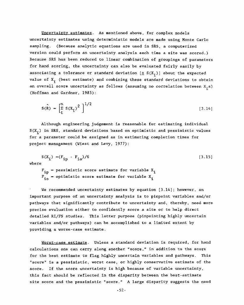
Uncertainty estimates. As mentioned above, for complex models uncertainty estimates using deterministic models are made using Monte Carlo sampling. (Because analytic equations are used in SRS, a computerized version could perform an uncertainty analysis each time a site was scored.) Because SRS has been reduced to linear combination of groupings of parameters for hand scoring, the uncertainty can also be evaluated fairly easily by associating a tolerance or standard deviation [.+ S(Xi)] about the expected value of Xi (best estimate) and combining these standard deviations to obtain an overall score uncertainty as follows (assuming no correlation between X.s) (Hoffman and Gardner, 1983):
1
A
[3.14]
Although engineering judgement is reasonable for estimating individual S(Xi) in SRS, standard deviations based on optimistic and pessimistic values for a parameter could be assigned as in estimating completion times for project management (Wiest and Levy, 1977):
S(Xi) =(F - Fio)/6 [3.15]
F - pessimistic score estimate for variable X i
iP where
i iP - optimistic score estimate for variable X We recommended uncertainty estimates by equation [ 3 . 1 4 ] ; however, an
important purpose of an uncertainty analysis is to pinpoint variables and/or pathways that significantly contribute to uncertainty and, thereby, need more precise evaluation either to confidently score a site or to help direct detailed RI/FS studies. This latter purpose (pinpointing highly uncertain variables and/or pathways) can be accomplished to a limited extent by providing a worse-case estimate.
Worst-case estimate. Unless a standard deviation is required, for hand calculations one can carry along another "score," in addition to the score for the best estimate to flag highly uncertain variables and pathways. This "score" is a pessimistic, worst case, or highly conservative estimate of the score. this fact should be reflected in the disparity between the best-estimate site score and the pessimistic "score." A large disparity suggests the need
If the score uncertainty is high because of variable uncertainty,
- 5 2 -
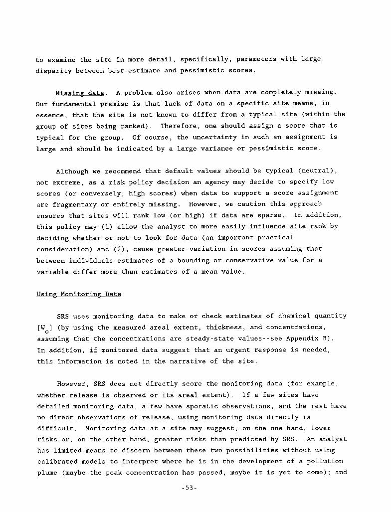
L
to examine the site in more detail, specifically, parameters with large disparity between best-estimate and pessimistic scores.
Missing data. A problem also arises when data are completely missing. Our fundamental premise is that lack of data on a specific site means, in essence, that the site is not known to differ from a typical site (within the group of sites being ranked). typical for the group. large and should be indicated by a large variance or pessimistic score.
Therefore, one should assign a score that is Of course, the uncertainty in such an assignment is
Although we recommend that default values should be typical (neutral), not extreme, as a risk policy decision an agency may decide to specify low scores (or conversely, high scores) when data to support a score assignment are fragmentary or entirely missing. However, we caution this approach ensures that sites will rank low (or high) if data are sparse. In addition, this policy may (1) allow the analyst to more easily influence site rank by deciding whether or not to look for data (an important practical consideration) and ( 2 ) , cause greater variation in scores assuming that
between individuals estimates of a bounding or conservative value for a variable differ more than estimates of a mean value.
Using - MonitorinF Data
SRS uses monitoring data to make or check estimates of chemical quantity (by using the measured areal extent, thickness, and concentrations, [Wo]
assuming that the concentrations are steady-state values--see Appendix B). In addition, if monitored data suggest that an urgent response is needed, this information is noted in the narrative of the site.
However, SRS does not directly score the monitoring data (for example, whether release is observed or its areal extent). If a few sites have detailed monitoring data, a few have sporatic observations, and the rest have no direct observations of release, using monitoring data directly is difficult. Monitoring data at a site may suggest, on the one hand, lower risks or, on the other hand, greater risks than predicted by SRS. An analyst has limited means to discern between these two possibilities without using calibrated models to interpret where he is in the development of a pollution plume (maybe the peak concentration has passed, maybe it is yet to come); and
- 5 3 -
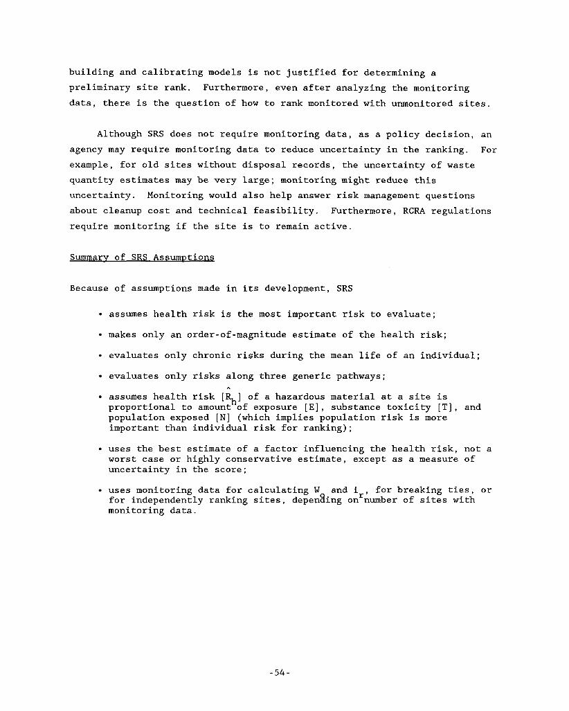
building and calibrating models is not justified for determining a preliminary site rank. Furthermore, even after analyzing the monitoring data, there is the question of how to rank monitored with unmonitored sites.
Although SRS does not require monitoring data, as a policy decision, an agency may require monitoring data to reduce uncertainty in the ranking. For example, for old sites without disposal records, the uncertainty of waste quantity estimates may be very large; monitoring might reduce this uncertainty. Monitoring would also help answer risk management questions about cleanup cost and technical feasibility. Furthermore, RCRA regulations require monitoring if the site is to remain active.
Summary of SRS Assumptions
Because of assumptions made in its development, SRS
assumes health risk is the most important risk to evaluate;
makes only an order-of-magnitude estimate of the health risk;
evaluates only chronic risks during the mean life of an individual;
evaluates only risks along three generic pathways;
assumes health risk [ R , ] of a hazardous material at a site is proportional to amount of exposure [E], substance toxicity [TI, and population exposed [N] (which implies population risk is more important than individual risk for ranking);
A
uses the best estimate of a factor influencing the health risk, not a worst case or highly conservative estimate, except as a measure of uncertainty in the score;
uses monitoring data for calculating W and i for breaking ties, or for independently ranking sites, depenaing on'kunber of sites with monitoring data.
- 5 4 -
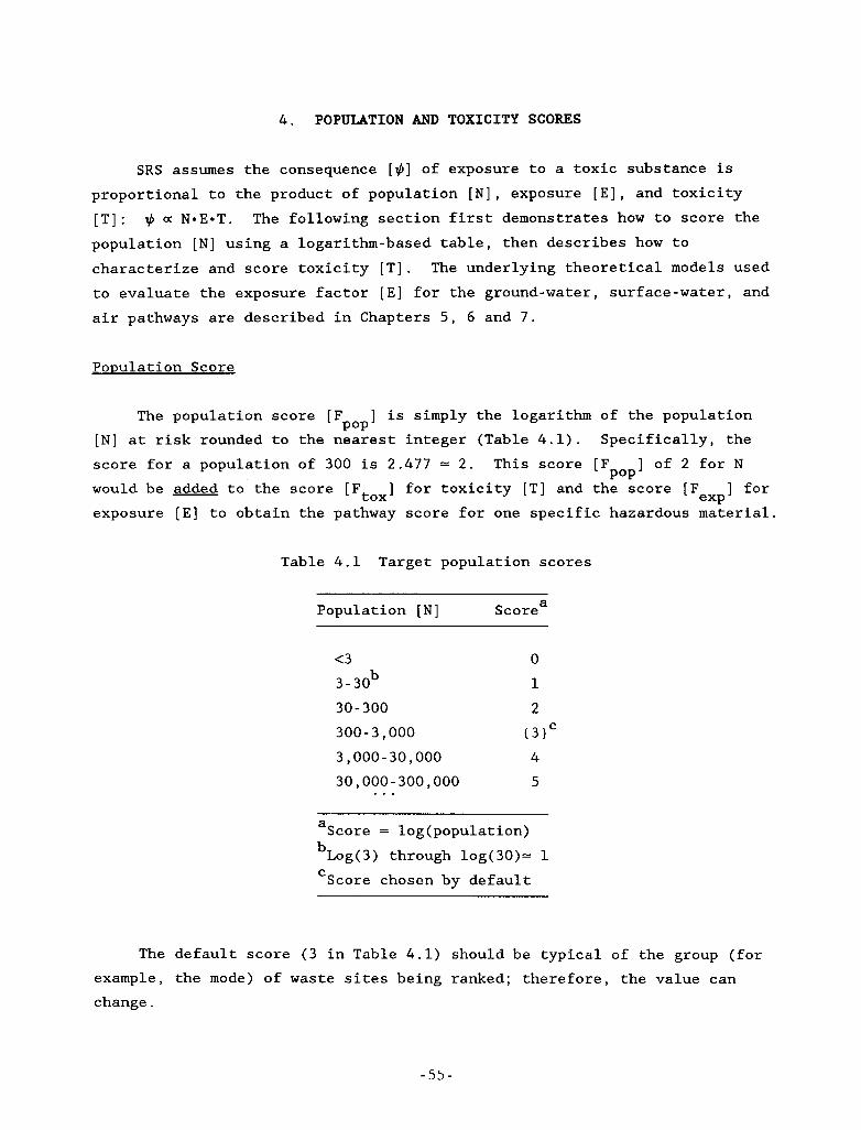
4 . POPULATION AND TOXICITY SCORES
-
c
c
SRS assumes the consequence [$I of exposure to a toxic substance is proportional to the product of population [N], exposure [E], and toxicity [TI: $ a N-E-T. population [N] using a logarithm-based table, then describes how to characterize and score toxicity [TI. The underlying theoretical models used to evaluate the exposure factor [E] for the ground-water, surface-water, and air pathways are described in Chapters 5, 6 and 7.
The following section first demonstrates how to score the
Population Score
The population score [F ] is simply the logarithm of the population [N] at risk rounded to the nearest integer (Table 4.1). Specifically, the score for a population of 300 is 2.477 = 2. This score [F ] of 2 for N would be added to the score [F 3 for toxicity [TI and the score [F ] for exposure [E] to obtain the pathway score for one specific hazardous material.
POP
POP tox exP
Table 4.1 Target population scores
a Population [N] Score
<3
3 - 3 0
30 - 300
b
300-3,000 ( 3 f 3,000-30,000 4 30,000-300,000 5 . . .
a Score = log(popu1ation) bLog( 3 ) through log( 30)- 1 Score chosen by default C
The default score ( 3 in Table 4.1) should be typical of the group (for example, the mode) of waste sites being ranked; therefore, the value can change.
-55- -
Clearly, the scoring is similar to other ranking schemes: It consists primarily of looking up values in tables. Yet, the theoretical basis of SRS
allows it to interweave with the overall goals of risk assessment. The real difficulty in SRS (or any ranking system) is selecting the parameter value (that is, collecting and interpreting the data).
The instructions provide guidelines for selecting parameter values, but these are stated primarily to provide consistency in estimating values from sparse data--important because many individuals will likely help rank the sites. (Presumably in needing SRS you have too many sites and too little time to do detailed investigations of every site, which usually implies that the task of ranking the sites is too large for one or a few specially trained individuals to complete in a reasonable amount of time.)
Consistency, however, does not always imply the most accurate technique is used. For example, the instructions specify the current population potentially exposed. Yet, one may correctly argue that for rapidly expanding areas the current population may be misleading. 10 years may better estimate the population exposed over the "long-term." Provided data exist to estimate the future population, the analyst may choose to ignore the guidelines to better estimate health risks.
The projected population in
We note that although both the health risk to an individual and the risk to the entire population can be important, we assume that for ranking a site the risk to the entire population is more important. This is a risk policy decision. (However, SRS does use the individual score, the score ignoring the population, as a tie-breaker in Chapter 8 )
Chronic Toxicity
The human health effect of a unit dose exposure to a chemical is evaluated from the chemical toxicity [TI. Two bases of chronic toxicity are used:
acceptable daily intake (ADI) for noncarcinogens, and
unit cancer risk (UCR) for carcinogens and radionuclides.
These toxicity measures are also used by EPA for the detailed RI/FS studies.
- 56-
-I -
_--
I
--
The acceptable daily intake (ADI) as defined in this report means the highest human intake of a chemical, expressed as mass of chemical per individual body mass per day, that does not cause adverse effects when exposed for a lifetime. (EPA uses the alternate term, reference dose [RfD] for ADI.) Although, many early ADIs were originally developed for assessing acute toxicity, the practical application of ADIs over the past 20 years has been in setting food and drinking water standards (chronic toxicity) (CWA, 1977). Health Effects Assessment (HEA) documents by the EPA Office of Research and Development are the recognized sources for ADIs on hazardous materials (Appendix C).
Toxicologists evaluate the AD1 for a chemical by applying a safety factor (to account for species differences and interspecies variation) to the experimentally estimated threshold dose (NOAEL). [Traditionally, noncarcinogenic chemicals are thought to have a threshold dose below which a toxic effect will not occur, the no-observed-adverse-effect level (NOAEL).] The safety factors vary: a 10-fold safety factor for long term human experiments; a 100-fold safety factor for well-conducted, chronic, animal experiments; and a 1000-fold safety factor for subchronic animal or lower- quality experiments (FSC, 1980).
The unit cancer risk (UCR) is the upper bound on lifetime risk of cancer per unit of dose, expressed as risk per mass of substance per individual body mass per day. (EPA uses the alternate term, carcinogenic potency factor [CPF] for UCR.) For carcinogens, toxicologists generally assume there is no threshold dose below which the substance will not cause cancer: level poses some risk of cancer. extrapolate from studies on animals at high doses to humans at low doses using a mathematical model, frequently linear (BEIR, 1980) [although much controversy surrounds the amount of conservatism in this approach (Runkle et al., 1981)].
any exposure To estimate the cancer risk, toxicologists
Although for chemical carcinogens, the UCR is often reported in HEA documents, cancer risk from radionuclides is usually reported by dose factors (ICRP, 1979; BEIR, 1980). We calculated equivalent UCRs (Appendix C) on the basis of these dose factors for use with SRS as follows.
. ..
-57-

Calculation of radionuclide UCR, Provided that the cancer risk [CR] per rem and the dose factor for either ingestion [DF ] or inhalation [DF ]
are known, the calculation of an equivalent UCR is straightforward: oral air
UCR - CR DForal * z where
CR = cancer risk per rem (cancer risk/rem)
DForal Z = weight (70 kg)
- dose factor from ingestion (rem per pCi/day)
Normally for radionuclides, the quantity [W ] is expressed in terms of its activity (Ci) rather than its mass (kg). For this case, Z converts UCR toxicity [TI expressed in units of (pCi/day)-l to (pCi/kg body mass/day) be consistent with AD1 toxicity.
0
-1 to
Runkle et al. (1981) tabulate dose factors for ingestion [DForal] and inhalation [DFair], assuming lifetime (70 yr) intake for numerous radioisotopes and the latent cancer risk per rem for several types of cancer. From these tables we calculated the ingestion or inhalation UCR listed in Appendix C by selecting an organ [b] (including the whole body) with the largest product of DF and CR.
ComDarinP: AD1 and UCR. As explained when defining AD1 and UCR, the assumptions toxicologists use to evaluate these measures of toxicity differ. However, they both attempt to evaluate chemical hazards. For use in SRS, the scales for the two measures of toxicity, UCR and ADI, must align such that a carcinogen (UCR) receiving a score of -5, for example, represents roughly the same risk as a noncarcinogen (ADI) receiving a score of -5. Aligning the scales requires finding the points representing acceptable risks for the two scales. This alignment is a policy choice, however, not a scientific one.
Acceptable cancer r i s k . Although not entirely consistent, regulations of the Food and Drug Administration (FDA) and Environmental Protection Agency (EPA) have generally considered lifetime cancer risks from individual chemicals of less than as insignificant and risks between 10 and as possibly significant but acceptable if technically infeasible or too costly to reduce further (for example, polychlorinated biphenyls (PCBs) and dioxin) (Rodricks et al., 1987). Consistent with this generality, EPA policy
- 6
-5%-
permits the aaizregate cancer risks after cleanup at Superfund sites to range anywhere from to (EPA, 1986b). We chose as representing a "very small" aggregate cancer risk from a waste site (Rodricks, 1984). [An incremental increase of 10 between a 0.2 to 0.3 chance of dying from cancer in the United States (Almanac, 1986)l.
- 5 is very small because a person currently has
A chance of contracting cancer approximates the middle ground for involuntary aggregate risks permitted in regulations. For example 10CFR20 (radiation protection standard) limits involuntary, whole-body radiation exposure to the public to 0.5 rem/yr (voluntary occupational exposure is 5 rem/yr) and 10CFR61 and 40CFR190 (low-level nuclear waste and nuclear power regulations) to 0.025 rem/yr. The latent cancer risk over a lifetime per rem of exposure for whole body exposure is about 1 . 5 ~ 1 0 - ~ (Runkle et al., 1981), thus the regulations correspond to risks of 7.5~10 and 3.75~10 , respectively, for involuntary exposure (and 10 for voluntary exposure).
-5 - 6
-3
Acceptable noncancer r i s k . We assumed that the health risk from a -5 lifetime AD1 exposure is also 10 . An AD1 for a noncarcinogen is
established such that the allowable dose poses no more than a very small risk of adverse effects. Unfortunately, we have no means of quantifying this "very small" risk. If one assumes that noncarcinogenic materials have a threshold dose below which the toxic effect will not occur, the no-observed- adverse-effect level (NOAEL), the risk is very small indeed.
However, we present the following two arguments to support our - 5 assumption of 10 . First, we simply argue that regulators have established
as an acceptable risk and AD1 levels are defined as acceptable. Second, (although admittedly more conservative than the threshold concept) we heuristically argue as follows. If, as an example, an animal study includes 1000 animals in the test group and at a certain extrapolated dose 1 animal is adversely affected in comparison to a control group; then there is a 0.1% risk near the NOAEL level. If a 100-fold safety factor is applied to the NOAEL, the risk is indeed (assuming a 1 to 1 dose response curve).
Aligning scales. If the assumptions concerning UCR and AD1 health risks are accepted, one can align the UCR and AD1 scales (Table 4.2). For example,
-59- L
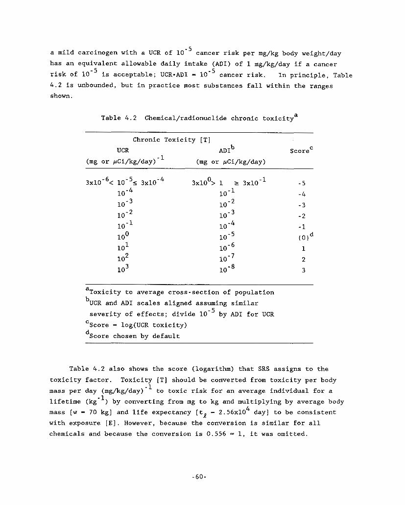
-5 a mild carcinogen with a UCR of 10 has an equivalent allowable daily intake (ADI) of 1 mg/kg/day if a cancer risk of is acceptable; UCR-AD1 = cancer risk. In principle, Table 4.2 is unbounded, but in practice most substances fall within the ranges shown.
cancer risk per mg/kg body weight/day
Table 4.2 Chemical/radionuclide chronic toxicitya
Chronic Toxicity [TI UCR A D I ~ ScoreC
(mg or pCi/kg/day) (mg 0'1: pCi/kg/day)
-1 3x1Oo> 1 1 3x10 10-1
-5 -4 -3 -2 -1
(Old 1 2 3
a
bUCR and AD1 scales aligned assuming similar Toxicity to average cross-section of population
severity of effects; divide by AD1 for UCR Score = log(UCR toxicity) C
dScore chosen by default
Table 4.2 also shows the score (logarithm) that SRS assigns to the toxicity factor. Toxicity [TI should be converted from toxicity per body mass per day (mg/kg/day)-' to toxic risk for an average individual for a lifetime (kg mass [w = 70 kg] and life expectancy [ta - 2.56~10 with exposure [E]. However, because the conversion is similar for all chemicals and because the conversion is 0.556 = 1, it was omitted.
-1 ) by converting from mg to kg and multiplying by average body 4 day] to be consistent
- 60-
5. GROUND-WATER SCORE
This chapter discusses the method used to evaluate the ground-water exposure score [E 1 . It starts by describing the idealized ground-water pathway and follows with the model underlying the SRS scoring. sections discuss the derivation and justification of this simple model, which you may wish to defer reading until later.
gw Subsequent
The ground-water pathway rarely can be ignored; it is frequently the most important contamination route. As shown by Table 2.1, ground-water contamination accounted for roughly 60% of the cases in the EPA survey (Lazar et al., 1976). The EPA also reported that nearly one-third of large, public ground-water systems in the United States show signs of chemical contamination, frequently from landfills (EPA, 1984a).
Idealized Ground-Water Pathway
The idealized ground-water pathway begins at a landfill (lagoons or injection wells involve simple modifications). Trapped moisture and precipitation vertically seeping into the landfill (no lateral seepage) react with the waste to form a leachate. This leachate escapes from the landfill by seeping through any degraded container and/or liner or fills and overflows the edges. It percolates vertically downward through the unsaturated zone to an aquifer (both assumed porous media). the aquifer either to a well down gradient from the landfill, where it is withdrawn, or to a stream that supplies drinking water (Figure 5.1).
The chemical is transported through
Understandably, actual sites may vary from this conceptual model. Unfortunately for the ground-water pathway, variations are not easily recognized without extensive site investigation. Furthermore, leakage of leachates into the potable aquifer may take years or decades to become apparent: First, leaching of the soluble and suspended waste is slow and often intermittent. Second, flow rates in the unsaturated zone and aquifer are slow, ranging from meters per day to meters per year. Consequently, an aquifer presumed isolated from waste in an initial scoring may later be polluted, for example, through an abandoned well. Herein lies the difficulty in scoring the ground-water pathway.
- 6 1 -
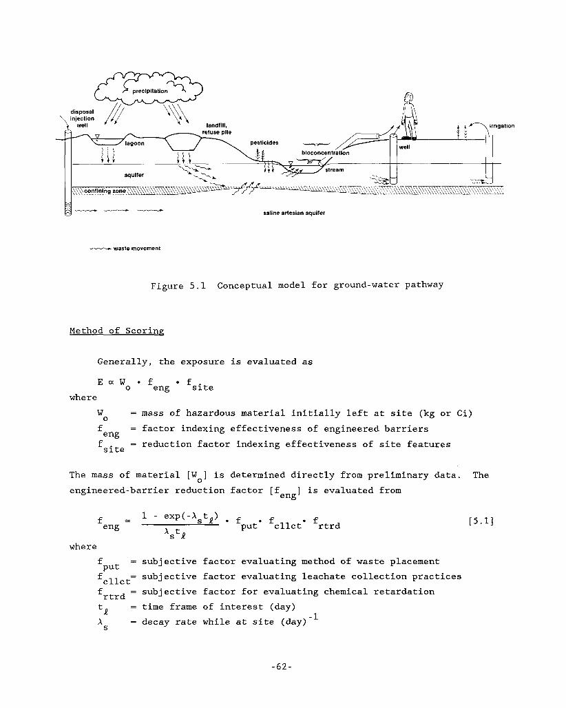
saline artesian aquifer
- waste movement
Figure 5.1 Conceptual model for ground-water pathway
Method of ScorinK
Generally, the exposure is evaluated as
o f E a '0 eng fsite where
= mass of hazardous material initially left at site (kg or Ci) wO f = factor indexing effectiveness of engineered barriers
fsite e*g
= reduction factor indexing effectiveness of site features
The mass of material [W ] is determined directly from preliminary data. The engineered-barrier reduction factor [f ] is evaluated from
0
eng
1 - exp(-Asta) . f = fput' fcllct' frtrd 2%
V R where
f = subjective factor evaluating method of waste placement Put
frtrd
= subjective factor evaluating leachate collection practices = subjective factor for evaluating chemical retardation = time frame of interest (day) = decay rate while at site (day)
fcllct
-1 A S
r 5 . 1 1
- 6 2 -
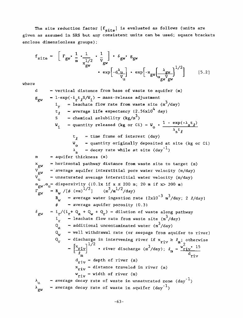
The site reduction factor [fsite] is evaluated as follows (units are given as assumed in SRS but any consistent units can be used; square brackets
enclose dimensionless groups):
'-.
fsite 1 m - . 1 ] hgw'
exP[-d+] x v gw
U where
d = vertical distance from base of waste to aquifer (m)
ggw r R 1 = 1-exp(-i t S / W . ) = mass-release adjustment
3 = leachate flow rate from waste site (m /day) = average life expectancy ( 2 . 5 6 ~ 1 0 ~ day)
r i
3 S = chemical solubility (kg/m )
1 - exp(-Xstn) Wi = quantity released (kg or Ci) = W 0
V R
15 .21
= time frame of interest (day) = quantity originally deposited at site (kg or Ci) = decay rate while at site (day-')
Wo
m = aquifer thickness (m) X = horizontal pathway distance from waste site to target (m) V = average aquifer interstitial pore water velocity (m/day) gw ,
gw = unsaturated average interstitial water velocity (m/day)
a
r = Bw / [ 4 (..a> 1/2 ] ( m3/rn1I2/day) ,au= dispersivity ((0.1~ if x I200 m; 20 m if x> 200 m)
gw gw -3 3
= average water ingestion rate (2x10 m /day; 2 ,!/day) BW 4 = average aquifer porosity (0.3)
6 = ir/(ir+ Qa + Qw + Qr) = dilution of waste along pathway 3 gw
= leachate flow rate from waste site (m /day) = additional uncontaminated water (m /day) = well withdrawal rate (or seepage from aquifer to river)
3 r i
Qa Qw
in intervening river if x 2 Rm; otherwise r iv river discharge (m 3 /day); R = w2 riv 15
m 3 A - m dr iv = depth of river (m)
a r iv
X = distance traveled in river (m) W = width of river (m)
= average decay rate of waste in unsaturated zone (day-') = average decay rate of waste in aquifer (day-')
r iv r iv
x gw
-63-
Nine major assumptions used to arrive at equation [5.2] are as follows:
Steady-state conditions appropriate for ranking chronic risks,
Degradation of the toxic waste is represented by first-order decay.
A mixing cell appropriately represents leaching of the waste.
1-D, vertical, saturated, waste transport occurs in unsaturated zone.
2-D, horizontal transport applies (vertical mixing occurs rapidly).
An individual's life expectancy (70 yr) is time frame of interest
Solubility [SI of the chemical indexes initial concentration [C 3
Hydrodynamic dispersion [D] approximated by aV; D unimportant. 0 *
Constant concentration injected into aquifer.
The SRS scores for the multiplicative factors of equation [5.2] are simply the logarithms of those factors rounded to the nearest integer. The instructions in Chapter 8 describe how to estimate these various parameters and provide tables for scoring. In addition, worksheets in Appendix A help an analyst organize data and properly combine scores. These scoring tables and worksheets make use of SRS much more straightforward than might initially appear from equations [ 5 . 1 ] and [5.2].
EPA has developed methods for assessing, in emergencies, exposure from accidental contamination of ground water or air (Cowherd et al., 1985; Donigian et al., 1983). Ideally, an assessor can gather information and evaluate one pathway in less than 24 hr. The formulas are similar to [5.1] and [5.2] and those described in the next two chapters, but they incorporate more detail on transport phenomenon. However, the rapid assessment methods are readily adapted to SRS, should an analyst wish more detail.
Derivation of Scoring Model
The ground-water migration of contaminants from a waste site to a downgradient target is conveniently divided into several segments. following sections describe these segments (source term, unsaturated zone transport, aquifer transport, and withdrawal) in more detail. The end results are formulas [5.1] and [5.2] that indicate important parameters to score and the way to combine these scores. (Table 2 . 1 ) , the discussion assumes a landfill waste site.
The
Because landfills are slightly more prevalent
- 6 4 -
Engineered-barrier factor. Engineered barriers serve to
extend the containment of the chemical (beneficial if decay occurs),
lower the release rate,
minimize human access to waste in the near term.
I They do not, however, provide indefinite isolation unless decay is complete, especially for the ground-water route.
I
.I.
The expression for the engineered-barrier reduction factor [f 1 , equation [ 5 . 2 ] , contains an analytic expression and three subjective factors. Because the quantity of waste escaping from the site can differ from that initially placed [Wo], if the waste can decay while held at the site, we corrected the waste quantity by (1-exp(-X t ) ) / A t ) , where X is the decay rate while at the site (day many sites and waste material this correction will be minor.
eng
s a s a S -1 ) and ta is the time frame of interest. For
The subjective factors (f and frtrd) adjust the score to account for transient effects of waste release. As is described later, SRS is based on steady-state formulas describing waste transport because transient phenomena have little effect on the ultimate risk to the public for surface and near- surface waste sites. As a result, parameters influencing time until exposure, such as retardation properties and waste placement, are not explicitly accounted for. ultimate risk, they do have importance in setting priorities for remedial action. For example, reduced mobility is important in delaying the extent of contamination. Thus, if two sites score identically except that the primary hazard at one site involves a chemical easily retarded, then the other site should have priority in cleanup, even though the ultimate risk is the same and might eventually make cleanup at both sites necessary.
Put
Although these parameters have no influence on the
Besides accounting for time to exposure, the placement reduction factor
3 also partially accounts for the probability of failure. For example, Lfput storage of liquid wastes in lagoons is more likely to lead to contamination than storage of stabilized waste in engineered landfills. Consequently, sites with poor waste placement should be penalized.
- 6 5 -
The subjective reduction factors acknowledge these facts and apply a small reduction in score. The reduction is small because, though the risk may be delayed, the ultimate risk is the same. Because the factors cannot be "derived," they are not defended further here but are adequately described in the instructions, Chapter 8 .
Chemical decav rate. In equation [5.2], the decay rate is needed. The average decay rate of the waste is also used in subsequent calculations and is, thus, discussed in general here. The decay rate is
= (In 2)/t1/2 where
= half-life of waste (day) 5/2
Persistence is a general term describing the length of time a hazardous waste remains in the environment in its toxic form. With radioactive wastes, the persistence is simply described by the radioactive half-life [tl/*]. toxic metals, the persistence is infinite, unless innocuous compounds can form. For inorganic or organic compounds, persistence describes the tendency to degrade into other chemical compounds or species, presumably less toxic. Common processes of degradation are (Verschueren, 1 9 8 4 ; Sax, 1 9 7 5 )
With
Biodegradation--enzymatic breakdown by microorganisms, typically bacteria, that can extract energy from the waste--occurs primarily in surface water and in upper layers of soil. metabolic rates and population density which, in turn, are functions of availability of other nutrients, pH, temperature, and sunlight.
Hydrolysis--addition or substitution by the OH- radical--may be the primary route of degradation in ground water. It is significant in surface water and a possible method in air. dependent on water pH, yet concentrations of constituents and rate constants are also important.
Rates are a function of
Rates are highly
Oxidation--attack by various oxygen species--is common in air (ozone or hydroxyl radical) and surface water (alkyl or peroxyl radicals). Reaction rates are controlled by concentration and rate constants.
Photolysis--breakdown through the action of light, usually sunlight-- may include light-catalyzed oxidation (photo-oxidation). in air, shallow surface waters, and on exposed soil. Rates depend on intensity of various spectral components (photon availability), concentrations, light absorption coefficient, and rate constants.
It occurs
- 6 6 -
This cursory review of degradation processes readily indicates that for many non-radioactive materials the persistence is pathway- and media- specific; hence, the analyst must approximate an average degradation rate (or equivalent half-life) for each medium. For example, for the ground-water pathway, an average degradation in the unsaturated zone and aquifer is needed. Under usual conditions this would be the biodegradation half-life in the unsaturated zone and the hydrolysis half-life in the aquifer. Furthermore, for the surface-water route, degradation from oxidation and hydrolysis would be important, and for the air route, photolysis. (However, the air-pathway model does not explicitly assume degradation in air.)
Because quantitative data on decay rates for specific chemicals are sometimes difficult to find, qualitative descriptions are also supplied for scoring. But, as a default, SRS assumes no degradation (or alternatively, the decay products are as toxic as the original waste material).
Leachate source term. The leachate is formed by infiltrating precipitation mixing with the waste. The quantity of leachate depends on the quantity of precipitation reaching the waste, which in turn depends on whether the site is open or closed. Apart from infiltrating precipitation, the initial quantity [Wo] (or concentration [Go]) and solubility [SI of the waste are the most important factors affecting leachate composition.
To develop a simple analytic model for the chemical source, assume that the lagoon or landfill behaves as a well-mixed chemical reactor with a fixed waste inventory. The release rate as leachate [dM/dt] at any given time is then (Weber, 1972) (units as assumed in the scoring system)
dM/dt = Ciir exp(-irt / n )
'i = '0 feng Co f = engineered-barrier reduction factor (equation [5.2]) S = chemical solubility (kg/m )
where 3
= chemical concentration at release (kg/m ) 3 - starting concentration 2: S (kg/m )
3 eng
3 i t = time after start of release (day)
= flow rate at which leachate leaves the site (m /day) r
- 6 7 - -
3 n = waste cell volume = W,/S (m ) I 1 - exp(-Xsta)
= quantity released (kg or Ci) = Wo ‘i XStR
tR = time frame of interest (day) W = quantity originally deposited at site (kg or Ci) A s = decay rate while at site (day) 0 -1
Although some liquid pollutants can move independently of the water phase, we assume that human health risk is better indexed by concentrations of soluble pollutants. Yet, except possibly for lagoons (surface impoundments), Co will likely be unknown. becomes the surrogate of starting concentration [C 1 .
Consequently, solubility [SI
0
As used in SRS, the exponential term [1-exp(-i t S / W . ) ] (hereafter termed the mass release adjustment [g]) mathematically determines whether the correct average release rate over period t is Sei or Wi/tn. This fact is readily seen by noting that for small i S / W
and as S/Wi --t a, l-exp(-irtaS/W.) + 1.
r R 1
a r l-exp(-irtaS/wi) = i t S/W r i’ r R i’
1
In the above expressions, we assumed the waste container released waste immediately because their life is usually less than 3 years. Accounting for container life could be important, however, in evaluating proposed sites using advanced technology containers. For these long-life containers, would be reduced by exp(-XcLc) where Xc is the decay rate while in the container (possibly different than normal decay) and L is the average life of the container before leaking. This reduction would be in addition to that already accounted for in equation [5.3].
wO
C
Equation [5.3] can be integrated from start of release, t = 0, to time 4 of interest, t = t (2.56~10 day), assuming i independent of time, to
evaluate the total mass released [MI: R r
M = Cin [l - exp(-irtR/ n )I [5.41
For a landfill, ir is the most difficult term to evaluate in equation [5.4], assuming site-specific percolation data are lacking. The flow rate from the waste site [i ] equals the surface area of the waste site capturing precipitation [A ] times the precipitation infiltrating [r ] into the landfill. Evaluating r
r S seep
from site-specific lysimeter data is the most seep
- 6 8 -
desirable method, but the data are likely lacking. Thus, a percentage of annual precipitation (or conductivity of a low permeability cover) is used.
Unsaturated-zone transDort. Once it escapes from the landfill, the contaminant is assumed to travel vertically downward through the intervening geologic strata to the aquifer. intermittently, transport in a saturated condition is assumed. Furthermore, because SRS evaluates the long-term human health risk, steady-state conditions are assumed to prevail. The partial differential equation describing the transport is (Javandel et al., 1984)
Although possibly occurring only
ac at
E - D. .ac a cvi
where C - contaminant concentration Dij ‘i x = spatial coordinate i
- dispersion tensor - interstitial velocity in ith spatial direction
The one-dimensional, steady-state solution to equation [ 5 . 5 ] , with initial condition of C(x,O) = 0; far boundary condition of aC(co,t) /at = 0 ; and input condition of C(0,t) = C is then (van Genuchten and Alves, 1982) i’
where
‘a ‘r DU d
vu
tl
= concentration injected into aquifer (kg/m 3 )
= average release concentration = M /(t i ) (kg/m 3 ) 2 R r
= saturated hydrodynamic dispersion in unsaturated zone (m /day)
= vertical distance from landfill or lagoon to aquifer (m) = percolation velocity in pores = r (m/day) /dJ perc r = percolation rate 4 = effective porosity in unsaturated zone (0.3) perc
= hydraulic gradient (1) = average decay rate in unsaturated zone (soil) (day -1 )
For persistent waste (no decay), there is no reduction in the chemical concentration under steady-state conditions, regardless of distance. Thus, the unsaturated zone, where transport is primarily one dimensional, offers no protection for persistent chemicals in the very long term when seepage is
- 6 9 -
possible (Piver and Lindstrom, 1984). However, as explained previously, we account for delayed risk by the subjective terms in equation [5.2].
For waste (primarily organic and radioactive) that does degrade, a site sufficiently high above the water table can safely detain the waste. This is the basis for septic tanks and their accompanying drain fields, which depend on aerobic bacteria in the tank and unsaturated zone to degrade the biologic waste. Thus, old empirical rules for locating waste disposal sites weighted the depth-to-water table factor heavily. For example, the LeGrand empirical point system (LeGrand, 1964) for evaluating potential pollution weighted the distance-to-the-water-table factor such that it could contribute up to 27% of the score irrespective of decay rates. Also, HRS (40CFR300) had this factor contribute up to 37% of the maximum exposure score, also irrespective of decay rate (score not including the effect of population).
The influence of the exponential term of equation [5.6] is indexed for the scoring system as follows: First, substitute into equation [5.6] the approximation of the hydrodynamic dispersion, assuming molecular diffusion is unimportant :
* D = u4D / T + aV = QV
where 2 D*
V = seepage velocity (m/day) Q = dispersivity (m) T = tortuosity (J3) 4 = average porosity (0.3) v = constrictivity (1)
= molecular diffusion (m /day)
2 Second, when 4D X /V unsaturated zone), equation [5.6] reduces to simple decay for slug flow,
(-4aXU/VU ) is much smaller than one (often true in u u u
= cr exp { -dXu/Vu) ‘a
When 4DUX/V: is much larger than one (often true in the saturated zone), equation [5.6] reduces to
[5.81
-70-
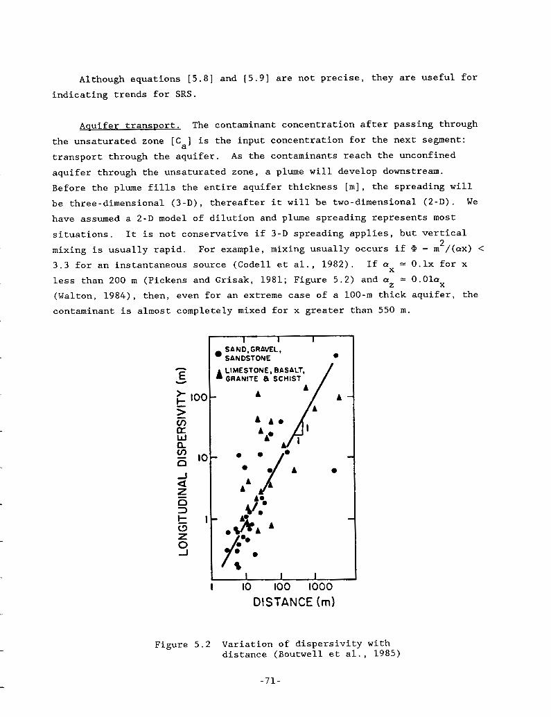
e.-
-
-
n
Y E g 100- - > 5 U w n cl -I 10-
z 3 I-
z 0 -I
a z i i5
Although equations [5.8] and [5.9] are not precise, they are useful for
indicating trends for SRS.
I I I SAND, GRAVEL,
A LIMESTONE, SANDSTONE BAS/ e GRANITE a SCHIST
A A
A A e
A A A*
A *{*A
A
I -
Aquifer transport. The contaminant concentration after passing through
the unsaturated zone [C 3 is the input concentration for the next segment: transport through the aquifer. aquifer through the unsaturated zone, a plume will develop downstream. Before the plume fills the entire aquifer thickness [m], the spreading will be three-dimensional (3-D), thereafter it will be two-dimensional (2-D). have assumed a 2-D model of dilution and plume spreading represents most situations.
a As the contaminants reach the unconfined
We
It is not conservative if 3-D spreading applies, but vertical
mixing is usually rapid. For example, mixing usually occurs if @ = m 2 /(ax) < 3 . 3 for an instantaneous source (Codell et al., 1982). less than 200 m (Pickens and Grisak, 1981; Figure 5.2) and aZ '-. 0 . 0 1 ~ ~ ~ (Walton, 1984), then, even for an extreme case of a 100-m thick aquifer, the contaminant is almost completely mixed for x greater than 550 m.
If ax = 0 . 1 ~ for x
Figu
.-
- I IO I00 1000
DISTANCE (m)
e 5.2 Variation of dispersivity w-th distance (Boutwell et al., 1985)
- 7 1 -
If one assumes 1) a line source (for example, well injection), 2) two- dimesional geometry, 3 ) zero lateral distance [y] (directly downgradient from site), and 4 ) transverse hydrodynamic dispersion [D ] equals one-fourth longitudinal dispersion [D ] (Freeze and Cherry, 1979; Table 5.1), then the analytic solution to the advection-dispersion transport equation [5.5] is (Wilson and Miller, 1978),
Y X
where 3 C = concentration in plume (kg/m )
D = hydrodynamic dispersion in aquifer (m /day) M = average mass injection rate per aquifer thickness [m]
P 2 gw
gw = C i /m (kg/day/m) a r
x = horizontal distance from site to target population [N] (m) V = aquifer seepage velocity = q Kgw/f$ (m/day) gw gw
K = average hydraulic conductivity through aquifer (m/day) 9 = hydraulic gradient
gw
X
f$ = average porosity ( 0 . 3 )
= average decay rate in aquifer (day-') gw
Equation [5.9] is similar to the 1-D, steady-state equation [5.6] except for the added terms in the denominator (especially x 'I2) which describe the
added diffusion in two dimensions. Simplifying equation [5.10] using equations [5.7] and [5.9] and omitting the expression to the 1/4 power (when this expression is important, its value in the exponential expression will dominate) results in
[5.11]
Withdrawal. Equation [5.11] expresses the concentration in the steady- state contaminant plume. aquifer disturbs the plume; hence, the well will likely withdraw both
The withdrawal of this contaminated water from an
-72-

Table 5.1 Dispersivities [a] reported in the literature (Pettyjohn et al., 1982)
Aquifer type Location Dispersivitv (m) a X ax/ay
-- Local Scale Alluvial sediment
Regional Scale Alluvial sediment
Glacial deposits
Fractured basalt
Limes tone
Chalk River, Ontario Lyons, France Barstow, CA Tucson, AZ
Rocky Mt. Arsenal, CO Color ado Sutter Basin, CA California Alsace, France
Long Island, NY Alberta, Canada
Hanford Site, WA Idaho
Culter area, FL Brunswick, GA
0 . 3 4 - 1 5 - 12 15 15
30 30
30 15
2 1
80 - 2000
3 - 61
30 9 1
22 6 1
0 . 3 4 - 780
1 3 10
3 15
5 5
10 3
contaminated and uncontaminated water, which results in some further dilution. This dilution is most easily represented as
Cw C i /(i,+QJ P r
Cw i r Qw
where 3
= withdrawal concentration (kg/m )
= flow rate of leachate from waste site (m /day) = the volume rate withdrawn from the aquifer through well (m /day)
3
3
Other sources of water for dilution also exist. Should the contaminant discharge into a stream that supplies water to a town, rather than discharging directly into a town well, dilution by the stream (stream flow rate, Qr) will occur. water to the town, dilution will also occur; hence, the expression for dilution becomes
Should other clean water sources [Q,] also supply
c - 7 3 -
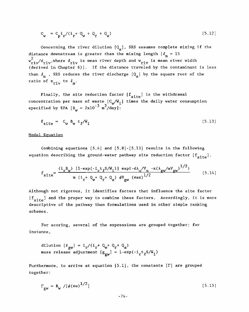
cw '-. c /(ir+ R + Q r + Qa) [5.12] P r
Concerning the river dilution [Q,], SRS assumes complete mixing if the distance downstream is greater than the mixing length [Rm = 15
,where driv is mean river depth and w is mean river width 2 r iJdr iv r iv W
(derived in Chapter 6)]. If the distance traveled by the contaminant is less than Rm , SRS reduces the river discharge [Q,] by the square root of the ratio of x to Rm. r iv
Finally, the site reduction factor [f ] is the withdrawal site concentration per mass of waste [Cw/wi] times the daily water consumption specified by EPA [Bw = 2x10 - 3 3
m /day]:
= Cw Bw tR/Wi [5.13] fsite
Model Equation
Combining equations [5.4] and [5.8]-[5.13] results in the following
site] equation describing the ground-water pathway site reduction factor [f
(irBw) [l-exp(-irtaS/wi)] exp( -dXU/VU -x(Xgw/aV [5.14]
1/2 m (2 + R+ Qr+ Qa> 4Vgw (.lrax> fsitez r
Although not rigorous, it identifies factors that influence the site factor
Lfsite descriptive of the pathway than formulations used in other simple ranking schemes.
] and the proper way to combine these factors. Accordingly, it is more
For scoring, several of the expressions are grouped together; for instance ,
dilution [ 6
mass release adjustment [ g ] = 1-exp(-i t S / w . ) 3 = ir/(i r + %+ Qr+ Qa) gw
gw r a 1
Furthermore, to arrive at equation [5.1], the constants [I'] are grouped together:
-74-
[5.15]
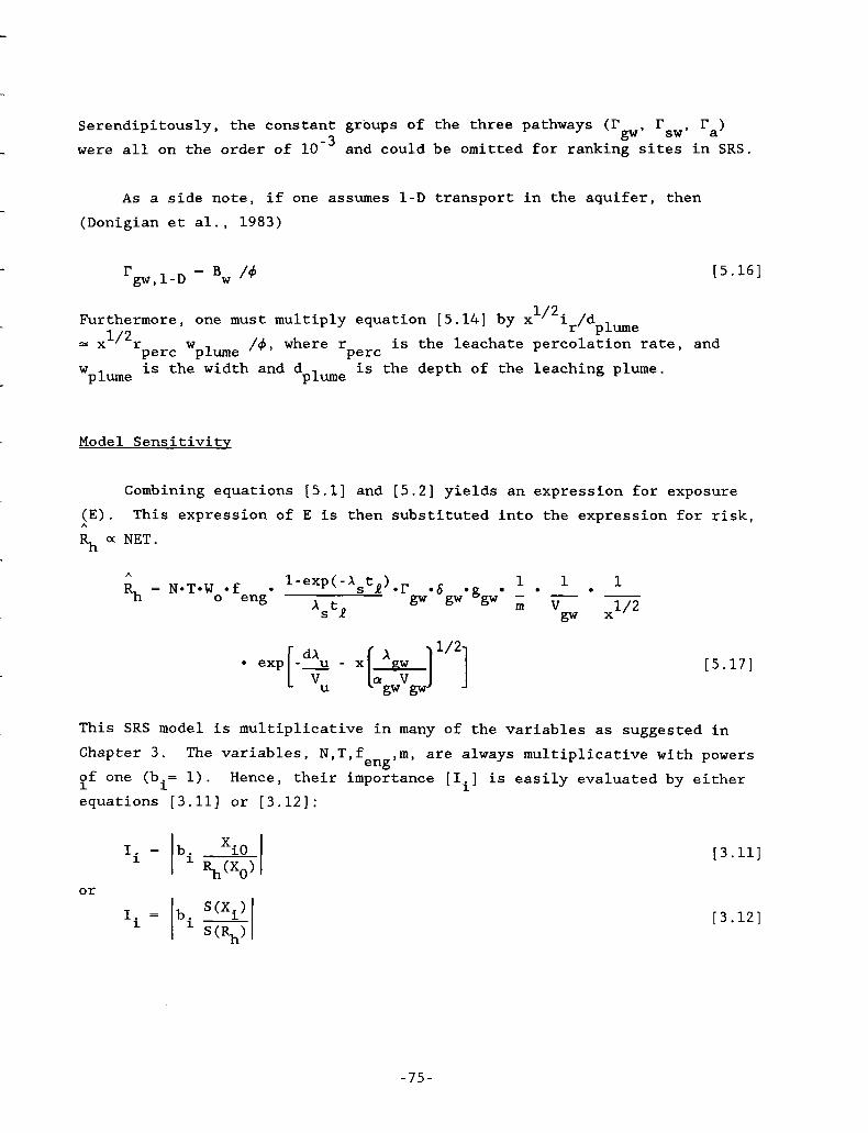
--
I_-
*-.
gw' I'sw, ra) Serendipitously, the constant groups of the three pathways (I' were all on the order of and could be omitted for ranking sites in SRS.
As a side note, if one assumes 1-D transport in the aquifer, then (Donigian et al., 1983)
I'gw,l-D Bw Id [5.16]
1/2. lr/dplume Furthermore, one must multiply equation [5.14] by x
==x 1/2
W plume
W rperc plume / d , where rperc is the leachate percolation rate, and is the width and dplume is the depth of the leaching plume.
Model Sensitivity
Combining equations [5.1] and [5.2] yields an expression for exposure (E). This expression of E is then substituted into the expression for risk, ;;h a NET.
[5.17]
This SRS model is multiplicative in many of the variables as suggested in Chapter 3. of one (b.= 1). Hence, their importance [I.] is easily evaluated by either 1 1 1 equations [3.11] or [ 3 . 1 2 ] :
The variables, N,T,feng,m, are always multiplicative with powers
or
[3.11]
[3.12]
The sensitivity of site risk to other variable groups in equation [5.17] varies somewhat based on variable values. As an example, examine the mass release adjustment [g 1 ,
gw
= 1-exp(-i t S/Wi) ggw r l
As a way to evaluate the influence of g we examined its importance at gw ’ acts like a switch (see
ggw its extreme values. At extreme values, discussion of equation [5.3]). hence, S has no influence. (The influence of i will be zero from g but its influence on the dilution term [6 ] could still be important.) On the other hand, if S and/or ir are very small, then g gw= - irtlS/wi. W influence of other variables at their extremes neglecting the range of uncertainty.
Provided S and/or ir are very large, gp= 1;
r gw
gw The influence of
drops to zero while S and ir have influence. Table 5.2 examines the 0
When waste decay [ A ] occurs the groupings dAU/VU (or d(Au/a V )1/2 and
x ( A@pgwVgw) difficulty analytically separating the influence of individual terms in the group except by noting the likelihood that their ranges vary and, thus, these groupings were not included in Table 5.2.
u u (or xApw/vgw) become very influential. An analyst has
-76-
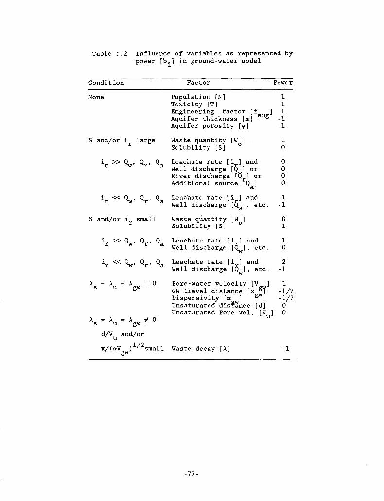
Table 5.2 Influence of variables as represented by power [bi] in ground-water model
Condition Factor Power
None Population [N] Toxicity [TI Engineering factor [f ] Aquifer thickness [m] eng Aquifer porosity [4]
S and/or ir large Waste quantity [Wo] Solubility [SI
i >> Qw, Qr, Qa Leachate rate [i ] and Well discharge [ or River discharge [ 1 or Additional source yQa]
i << Q r P Qa Leachate rate [i ] and Well discharge [ \ I , etc.
Waste quantity [Wo] Solubility [SI
r
r
S and/or ir small
i >> R, Qr, Qa Leachate rate [i ] and
i << 9J. Qr, Qa Leachate rate [i ] and
Well discharge [\I, etc.
Well discharge [ \ I , etc.
r
r
As = Xu = X - 0 Pore-water velocity [V ] gw GW travel distance [x gy
Dispersivity [a ] gw Unsaturated disgxnce [ d] Unsaturated Pore vel. [Vu]
1 1 1 -1 -1
1 0
0 0 0 0
1 -1
0 1
1 0
2 -1
1 - 1/2 - 1/2 0 0
X = A - A # O S u gw d/VU and/or
x/(aVgw)1/2small Waste decay [A] -1
- 7 7 -
6. SURFACE-WATER SCORE
This chapter discusses the method used to evaluate surface-water exposure [E 1 . It first describes the idealized surface-water pathway. It then presents the underlying model used by SRS for scoring. A subsequent section discusses the derivation of this simple model--a section you may wish to postpone reading.
sw
In the past, risk to humans or other biologic systems from surface-water contamination has been important. The EPA survey in 1977 (Lazar et al., 1976) found about 33% of the incidents involved surface-water contamination. Of these incidents, haphazard disposal on vacant property was the most frequent contaminant source (41%) (Table 2.1). This damage mechanism was assumed in the following development. Table 2.1 shows contami.nation from landfills and lagoons accounted for 29 and 25%, respectively; t5us with past waste sites, engineered disposal methods were also important sources of surface-water contamination. However, RCRA (1976) and supporting EPA regulations (40CFR267) should significantly reduce surface-water contamination at future engineered sites.
Idealized Surface-Water Pathway
The surface-water pathway begins at a site where toxic waste is exposed to the weather in the upper 0.1 m of soil (or entire lagoon). Precipitation falls on the area, dissolving some of the waste and eroding soil particles to which some of the toxic waste has adsorbed. The dissolved and sedimentary waste is transported overland to an intermittent stream, diluted with water from the same rainfall, transported to a graded perennial stream, diluted further, and finally drawn into a drinking water supply (Figure 6.1).
For SRS, no removal of sedimentary or dissolved waste is assumed while transported in the stream except that which can be expressed as a exponential decay. Further, all the adsorbed waste is assumed to have de-adsorbed from sediments before reaching the water-supply intake, consistent with our assumptions of steady state. Dissolved waste, however, may pass through the system more quickly than sedimentary waste, making decay more important in the latter case.
- 7 8 -
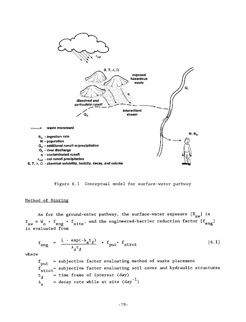
c
Y
--
/--- ___y
intermittent stream
/ / Qa
u waste movement
B, - ingestion rate N - population
Q, - additional runoff w/precipitation Q, - river discharge q - contaminated runoff
rne, - net runoff precipitation S, T, A , n - chemical solubility, toxicity, decay, and volume
Figure 6.1 Conceptual model for surface-water pathway
Method of Scoring
A s for the ground-water pathway, the surface-water exposure [E ] is sw and the engineered-barrier reduction factor [f ]
eng o f Esw a '0
is evaluated from eng fsite'
[6 .11 - 1 - exp(-Asta)
fput* fstrct - f V k ?
eng
where = subjective factor evaluating method of waste placement = subjective factor evaluating soil cover and hydraulic structures = time frame of interest (day) = decay rate while at site (day-')
Put f
strct
- 7 9 -
] are not derived, their and fstrct Because the subjective factors [f description is found in the instructions (Chapter 8).
Put
The site reduction factor [f ] is evaluated from one of two simple site expressions. For many wastes, either the dissolved or sediment transport route described above dominates; specifically, the partition coefficient [Kd] will be either near zero or orders of magnitude greater than one. Furthermore, because K is rarely precisely known, SRS considers only two cases: For K less than about 0.02 m /kg (corresponding to a retardation [R] less than loo), the substance is assumed to leave the site dissolved. For Kd greater than 0.02 m /kg, the substance is assumed to leave the site adsorbed on soil particles.
3 d d
3
Scoring. - for small partition coefficient. The hazardous substance is assumed to leave the waste site dissolved when K is small (less than 0.02 m /kg); this is the default case. For this case, groupings dimensionless)
d is (major 3
fsite
r x gsw . &SW - = - Bw
fsite r q a sw sw where
- 3 3 - human ingestion rate (2x10 m /day; 2 l/day) Bw = sw q - annual runoff from waste site - r net. :s (m3/day)
As = 1-exp(-qt S / W . ) = mass release adjustment
S = waste solubility (kg/m or Ci/m )
tR - average human life expectancy (2.56~10~ day) wi - wo 1 - exp(-Astl)
= surface area of contamination (m )
gsw 3 3 1 1
V l Wo = waste within 0.1 m of surface (kg or Ci) A s = decay rate while at site (day-')
r = mean daily precipitation at waste site (m/day) r = (ra- 0.2Sw) / (ra+ 0.8Sw) (m/day) 2 a net
Sw = a [(1000/CN) -101 - water retention factor -5 a - conversion constant ((7x10 ) for ra in m/day)
CN = Soil Conservation Service (SCS) runoff curve number = surface water velocity (m/day) vsw
- 8 0 -
....".
--
.-
-.-
X
CY
- distance traveled in water pathway from site to target (m) = 0.6 driv 5/6 - dispersivity in surface water (1 m )
= q/(q + Qa + Q,) - surface-water dilution factor
r iv sw
= mean depth in river dr iv sw 9
- waste xsw
flow rate of supplemental clean water (m'>/day) discharge .^ in river if x r iv 1 am - , otherwise
3 river discharge (m /day)
= mixing length (m) 2 m m = 1 5 Wriv / driv W = width of river (m) r iv decay rate in surface water (day-')
Scoring - for large Dartition coefficient. The hazardous substance is assumed to leave the site adsorbed on soil particles for large Kd (greater than about 0.02 m /kg). is For this case fsite 3
x = Bsw ssw fsite -
sw sd q v . 3 1
where h - soil depth subject to erosion each year (0.01 m/yr) Vsd = suspended sediment velocity--default is Vsw (m/day) Ys = 5 . 6 ~ 1 0 - ~ CP LS RE = annual sediment yield per area (kg/m2/yr)
CP = SCS control-practice factor LS = SCS slope factor RE = SCS rainfall factor
3 - surface soil bulk density (1500 kg/m 1 'b
S i x major assumptions used to arrive at [ 6 . 2 ] and [ 6 . 3 ] are as follows:
thorough mixing occurs in the surface water
degradation is properly represented by first-order decay
effect of waste decay is similar to that derived for ground water
partition of waste between adsorbed and dissolved phases is d represented by K
Universal Soil Loss Equation (USLE) (Barfield et al., 1981) adequately represents erosion at site
"-
SCS runoff equation (USBR, 1977) approximates annual site runoff
-81-
-- _I_-
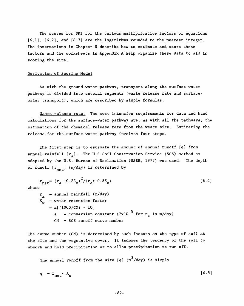
The scores for SRS for the various multiplicative factors of equations [6.1], [6.2], and [6.3] are the logarithms rounded to the nearest integer. The instructions in Chapter 8 describe how to estimate and score these factors and the worksheets in Appendix A help organize these data to aid in scoring the site.
Derivation of Scoring - Model
A s with the ground-water pathway, transport along the surface-water pathway is divided into several segments (waste release rate and surface- water transport), which are described by simple formulas.
Waste release rate. The most intensive requirements for data and hand calculations for the surface-water pathway are, as with all the pathways, the estimation of the chemical release rate from the waste site. release for the surface-water pathway involves four steps.
Estimating the
The first step is to estimate the amount of annual runoff [q] from annual rainfall [ra]. adapted by the U.S. Bureau of Reclamation (USBR, 1977) was used. The depth of runoff [met] (m/day) is determined by
The U.S Soil Conservation Service (SCS) method as
net- r where
r - a sW
2 (ra- 0.2Sw) /(ra+ 0.8Sw)
annual rainfall (m/day) water retention factor a[(1000/CN) - 101 a = conversion constant (7x10 for ra in m/day) CN = SCS runoff curve number
-5
~6.41
The curve number (CN) is determined by such factors as the type of soil at the site and the vegetative cover. It indexes the tendency of the soil to absorb and hold precipitation or to allow precipitation to run off.
3 The annual runoff from the site [q] (m /day) is simply
net. As q = r
-82-
v.51
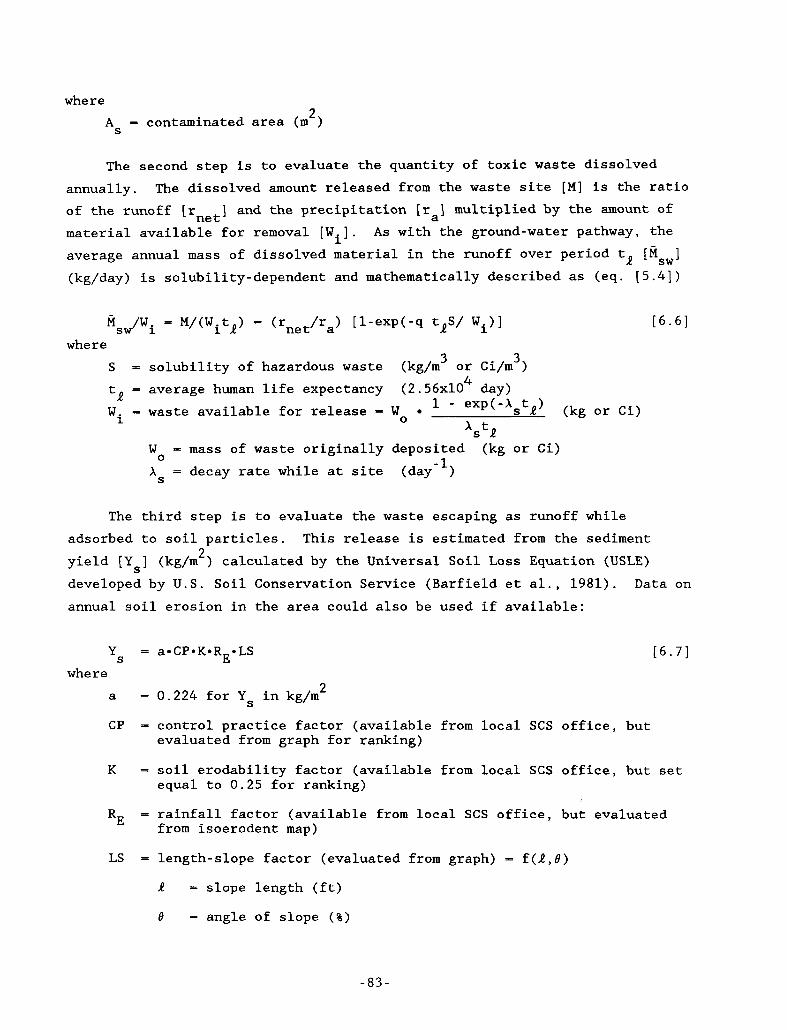
c-
where 2 As = contaminated area (m )
__._
The second step is to evaluate the quantity of toxic waste dissolved annually. The dissolved amount released from the waste site [MI is the ratio of the runoff [met] and the precipitation [r 3 multiplied by the amount of material available for removal [Wi]. As with the ground-water pathway, the average annual mass of dissolved material in the runoff over period tR [Msw] (kg/day) is solubility-dependent and mathematically described as (eq. [5.41)
a
MSW/Wi = M/(WitR> = (rnet/ra> [l-exp(-q tQS/ Wi>l where
3 S - solubility of hazardous waste (kg/m3 or Ci/m )
tR = average human life expectancy (2.56~10 day) W. = waste available for release - Wo
4
(kg or Ci) 1 - exp(-Xsta) 1
V R Wo = mass of waste originally deposited As = decay rate while at site (day-')
(kg or Ci)
The third step is to evaluate the waste escaping as runoff while adsorbed to soil particles. This release is estimated from the sediment yield [Y,] (kg/m ) calculated by the Universal Soil Loss Equation (USLE) developed by U.S. Soil Conservation Service (Barfield et al., 1981). Data on annual soil erosion in the area could also be used if available:
2
Ys = a*CP*K*RE*LS where
2 a = 0.224 for Ys in kg/m
~6.71
CP - control practice factor (available from local SCS office, but evaluated from graph for ranking)
K = soil erodability factor (available from local SCS office, but set equal to 0.25 for ranking)
RE
LS = length-slope factor (evaluated from graph) = f(R,B)
= rainfall factor (available from local SCS office, but evaluated from isoerodent map)
R = slope length (ft)
B = angle of slope (%)
- 8 3 -
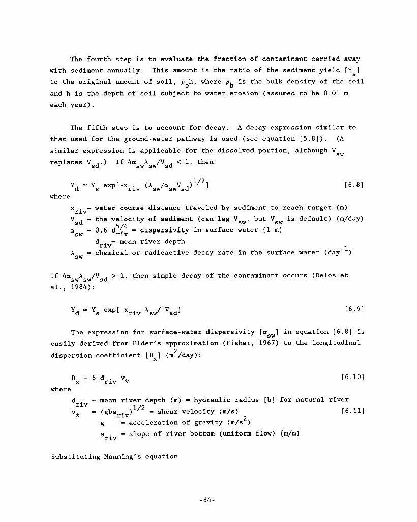
The fourth step is to evaluate the fraction of contaminant carried away This amount is the ratio of the sediment yield [Y,] with sediment annually.
to the original amount of soil, pbh, where p
and h is the depth of soil subject to water erosion (assumed to be 0.01 m each year).
is the bulk density of the soil b
The fifth step is to account for decay. A decay expression similar to
that used for the ground-water pathway is used (see equation [ 5 . 8 ] ) . (A similar expression is applicable for the dissolved portion, although Vsw
< 1, then replaces V sd') If 4aswXsw/Vsd
1/2 ] riv (Xsw/aswVsd) Y = Y exp[-x d s
where diment to re x - water course distance traveled by r iv ch target (m)
Vsd - the velocity of sediment (can lag Vsw, but Vsw is dezault) (m/day) a - 0 . 6 dzi: = dispersivity in surface water (1 m)
= chemical or radioactive decay rate in the surface water (day-')
sw = mean river depth dr iv
Xsw
If 4a X
al., 1 9 8 4 ) :
/vsd > 1, then simple decay of the contaminant occurs (Delos et sw sw
Yd = Ys exp[-x riv 'sw/ 'sd] ~ 6 . 9 1
The expression for surface-water dispersivity [a 3 in equation [ 6 . 8 ] is sw easily derived from Elder's approximation (Fisher, 1 9 6 7 ) to the longitudinal dispersion coefficient [Dx] (m /day): 2
D = 6 driv vJ: X
where [ 6 . 1 0 ]
= mean river depth (m) = hydraulic radius [b] for natural river = (gbsriV)l/* = shear velocity (m/s)
dr iv [ 6 . 1 1 ]
2 v*
g = acceleration of gravity (m/s )
S = slope of river bottom (uniform flow) (m/m) r iv
Substituting Manning's equation
-84-
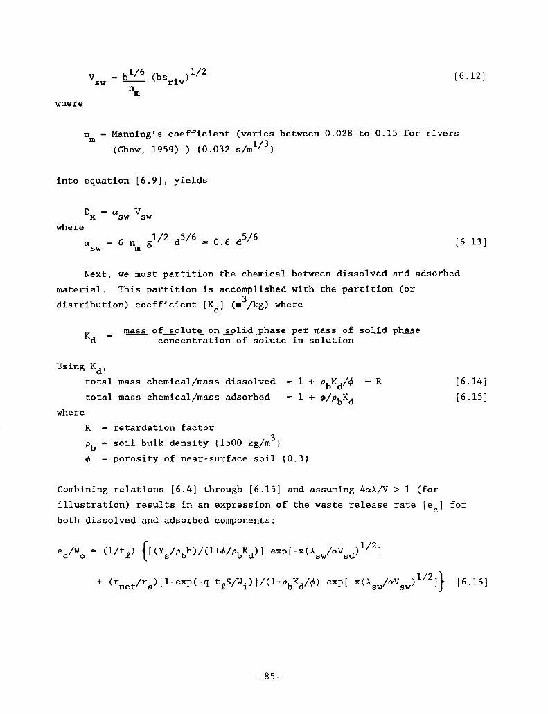
[6.12]
where
n = Manning's coefficient (varies between 0.028 to 0.15 for rivers 1/3 )
m (Chow, 1959) ) (0.032 s/m
into equation [6.9], yields
sw vsw D = a X where
[6.13]
Next, we must partition the chemical between dissolved and adsorbed material. This partition is accomplished with the partition (or distribution) coefficient [Kd] (m /kg) where 3
mass of solute on solid phase Der mass of solid phase Kd == concentration of solute in solution
Using Kd, total mass chemical/mass dissolved - 1 + pbKd/d = R total mass chemical/mass adsorbed 5 1 + d/pbKd
where R = retardation factor pb = soil bulk density (1500 kg/m )
d = porosity of near-surface soil (0.3)
3
[6.14] [6.15]
Combining relations [6.4] through [6.15] and assuming 4aX/V > 1 (for illustration) results in an expression of the waste release rate [e ] f o r
both dissolved and adsorbed components: C
-85-
Surface-water transport. For surface-water transport, toxic waste is assumed to be thoroughly mixed with river water after traveling the mixing length Rm; hence, the main phenomenon occurring with transport of the toxic waste is dilution. The withdrawal concentration [Cw] after dilution of the chemical release is thus
Cw = e /(q + Qa + Qr) [6.17] C
where
Qa = supplemental clean water (usually zero) Qr = river discharge if x r iv 2 am;
otherwise X 3 Qr = riv river discharge (m /day)
r iv 2 'm
Rm = 15 w / driv = mixing length (m) = mean river depth (m) dr iv
W = mean river width (m) r iv
If the distance traveled by the contaminant is less than Rm, SRS reduces the river dilution [Q ] by the square-root of the ratio of x to Rm (Codell et r r iv al., 1982) .
The above expression for mixing length [I ] is easily approximated as m follows.
2 R = a V w m sw riv lDy [6.18] where
a = (0.3) for river-bank spill or injection (Codell et al., 1982)
2 = 0.1 for centerline spill (Hubbard et al., 1982)
- 0 . 2 drivv* - lateral dispersion coefficent (Fisher, 1967) (m /day) D Y
= mean surface-water velocity (m/day) vsw
Again using equations [6.10] and [6.11] yields
Rm = 0.3 Wriv 2 /(0.2 g d5/6)
If Manning's coefficient [n ] is again set equal to 0.032, then m
-86-
n L R = 1 5 ~ m r iv
Finally, the concentration per
ldr iv
site reduction factor [fsite] is the withdrawal mass of waste [Cw/w.] times the average daily water
q m 1 consumption [B W = 2xlO-’ m’/day] :
[6.19]
= cw Bw t p i [6.20] fsite
Model eauation. Combining equations [6.16], [6.17], and [6.20] yields the following equation describing the site reduction factor [f ] for the surface-water pathway (4aX/V > 1):
site
sd I BW fsite L tR (q + Qa + Qr)
1/2 + [l-exp[-qtl z ] ] ‘net 1 exp[-x[)isw ] I) [6.21]
a l+PbKd aVsw r ‘i
For SRS scoring, several of the parameters are grouped together:
dilution [SswI = q/(q + Qa + Qr> mass release adjustment [g ] = 1-exp(-qt S/W.) sw 1 1
Furthermore, SRS considers only two cases for Kd: Kd small or Kd very large. terms from equation [6.21] to obtain equation [6.2], assuming the hazardous material leaves the waste site dissolved in surface runoff.
3 large (greater than 0.02 kg/m ) , we omit the dissolution terms from equation [6.21] to obtain equation [6.3], assuming the hazardous material leaves the site adsorbed to soil particles.
3 For Kd small (less than 0.02 kg/m ) , we omit the sedimentary yield
For Kd very
7. AIR-PATHWAY SCORE
This chapter discusses the model underlying the air-pathway exposure Specifically, it describes the idealized air pathway, the scoring [E,].
model, and the derivation of this model.
Contamination via the air pathway was significant in only 4% of the cases reported by the EPA in its survey (Table 2.1) (EPA, 1977). Although only a survey, it does suggest this pathway is frequently unimportant. From Table 2.1, landfills with little cover or haphazard waste sites were the most prevalent source when contamination via the air pathway was important.
Idealized Air Pathway
The air pathway begins at the waste site. Hazardous waste, deposited directly onto the ground or covered with less than 10 m of soil, escapes directly into the air either because it is volatile or because wind suspends soil particles that can be inhaled (less than 10 pm diam.) to which waste is adsorbed. These chemicals are transported by wind currents to a nearby borough where they are inhaled by permanent residents (Figure 7.1).
Method of Scoriq
As with the other pathways, the air exposure [E ] is evaluated as a where engineered-barrier reduction factor [f ] is
eng fsite’ eng Ea a Wo f
where f = subjective factor evaluating method of waste placement
- time frame of interest (day) = decay rate while at site (day )
Put
-1
not being derived, are discussed in eng ’ The subjective factors comprising f the instructions (Chapter 8) . As with the other pathways, these factors adjust for sites with different exposure times and probabilities of contaminant release.
- 8 8 -
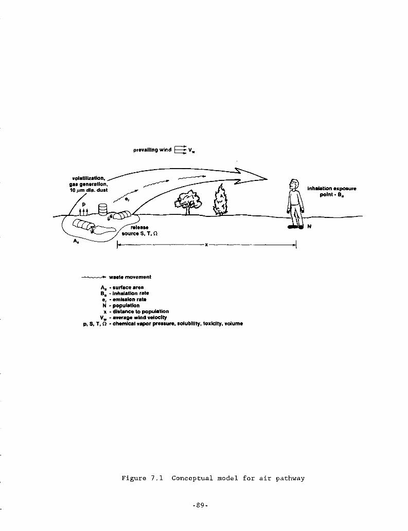
prevailing wind E V,
voiatllizatlon, gas generation,
- warte movement
A, - surface area B, - Inhalation rate e, - emirrion rate N - population x - distance to population
V, - average wind veioclty p, S, 1, C l - chemlcai vapor prcnrure. solubliity, toxlcity, volume
Figure 7.1 Conceptual model for air pathway
- 8 9 -
inhaiatlon exporure polnt - B,
N
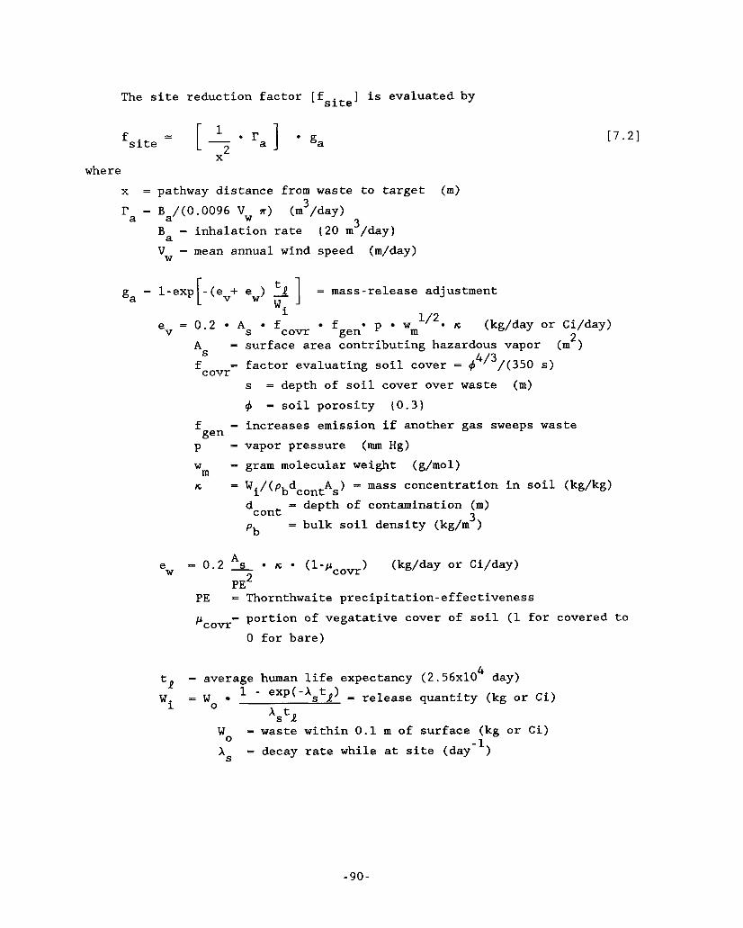
The site reduction factor [fsite] is evaluated by
1 fsite = [ - e r a 3 ] * g a [7.21
XL where
x = pathway distance from waste to target (m) Pa = Ba/(O .0096 Vw R) (m3/day)
Ba = inhalation rate Vw = mean annual wind speed
(20 m3/day)
(m/day)
= 1-exp -(e + e ) 2 = mass-release adjustment 'i
'I2* tc (kg/day or Ci/day)
ga L w ' 1 As fcovr fgen* P wm 2
e = 0.2 V As = surface area contributing hazardous vapor (m )
s = depth of soil cover over waste (m) 4 = soil porosity (0.3)
4 / 3 = factor evaluating soil cover - 4 /(350 s) covr
f = increases emission if another gas sweeps waste P - vapor pressure (mm Hg) W = gram molecular weight (g/mol) tc
gen
m = Wi/(pbdcontAs) = mass concentration in soil (kg/kg)
- depth of contamination (m) = bulk soil density (kg/m )
dcont 3 'b
A
PE2 e W - 0 . 2 s . n . (l-Pcovr> (kg/day or Ci/day)
PE = Thornthwaite precipitation-effectiveness - portion of vegatative cover of soil (1 for covered to "covr 0 for bare)
t, = average human life expectancy (2.56~10~ day) -
exp(-XstR) - release quantity (kg or Ci) 1 - n wi = wo
V R Wo = waste within 0.1 m of surface (kg or Ci) A s = decay rate while at site (day-')
- 90-
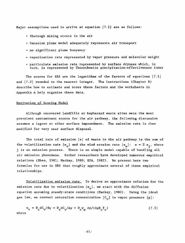
.’I
II
...I.
Major assumptions used to arrive ‘at equation [7.2] are as follows:
thorough mixing occurs in the air
Gaussian plume model adequately represents air transport
no significant plume buoyancy
vaporization rate represented by vapor pressure and molecular weight
particulate emission rate represented by surface dryness which, in turn, is represented by Thornthwaite precipitation-effectiveness index
The scores for SRS are the logarithms of the factors of equations [7.1] and [7.2] rounded to the nearest integer. The instructions (Chapter 8 )
describe how to estimate and score these factors and the worksheets in Appendix A help organize these data.
Derivation of Scoring Model
Although uncovered landfills or haphazard waste sites were the most prevalent contaminant source for the air pathway, the following discussion assumes a lagoon or other surface impoundment. The emission rate is then modified for very near surface disposal.
The total rate of emission [e] of waste to the air pathway is the sum of where all rical
the volatilization rate [e ] and the wind erosion rate [e 1 : e - X e j is an emission process. There is no simple model capable of handling air emission phenomena. Rather researchers have developed numerous emp relations (Shen, 1981; Mackay, 1980; EPA, 1982). We present here two formulas for use in SRS that roughly approximate several of these empir relationships.
V W j’
cal
Volatilization emission rate. To derive an approximate relation for the emission rate due to volatilization [ev], we start with the diffusion equation assuming steady-state conditions (Mackay, 1980). Using the ideal gas law, we convert saturation concentration [C ] to vapor pressure [p]:
V
n = DcdCv/dX = DcACV/Ax = D w Ap/(AxRcTc) V c m
where
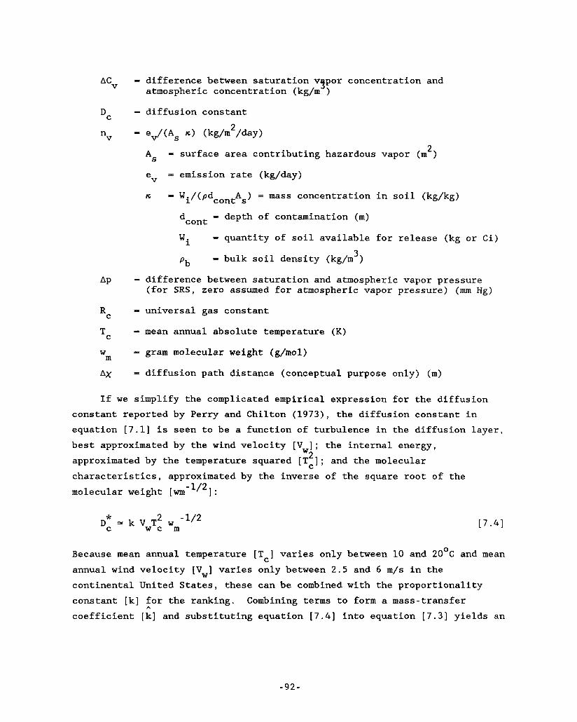
ACv - difference between saturation v;Spor concentration and atmospheric concentration (kg/m )
- diffusion constant DC
n V
2 = surface area contributing hazardous vapor (m ) As
e = emission rate (kg/day)
K,
V
- Wi/(pdcontAs) = mass concentration in soil (kg/kg)
= depth of contamination (m)
= quantity of soil available for release (kg or Ci)
= bulk soil density (kg/m )
dcont
'i
pb 3
Ap - difference between saturation and atmospheric vapor pressure (for SRS, zero assumed for atmospheric vapor pressure) (mm Hg)
- universal gas constant = mean annual absolute temperature (K)
TC
W - gram molecular weight (g/mol) A x = diffusion path distance (conceptual purpose only) (m) m
If we simplify the complicated empirical expression for the diffusion constant reported by Perry and Chilton (1973), the diffusion constant in equation [7.1] is seen to be a function of turbulence in the diffusion layer, best approximated by the wind velocity [V 1 ; the internal energy, approximated by the temperature squared [Tc]; and the molecular characteristics, approximated by the inverse of the square root of the
w2
molecular weight [wm -1/21.
* 2 -1/2 Dc = k VwTc wm
Because mean annual temperature [T ] varies only between 10 and 2OoC and mean annual wind velocity [Vw] varies only between 2.5 and 6 m/s in the continental United States, these can be combined with the proportionality constant [k] for the ranking. Combining terms to form a mass-transfer coefficient [k] and substituting equation [7.4] into equation [7.3] yields an
C
A
-92-
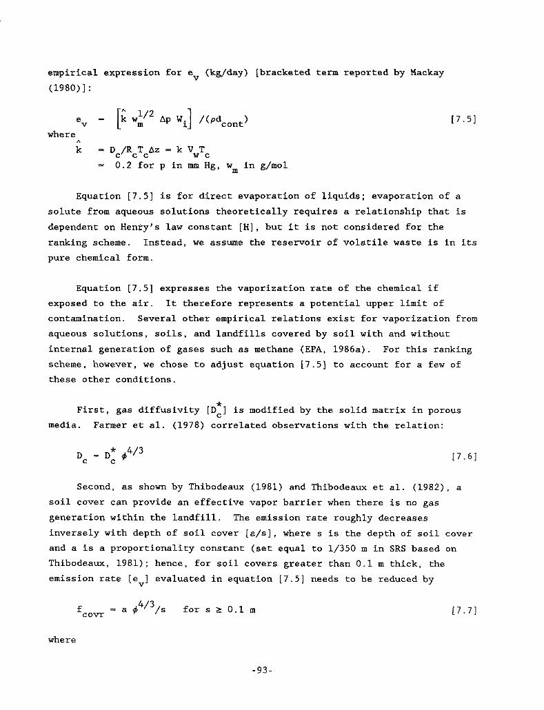
..I-
.”_.“
.-.~
empirical expression for ev (kg/day) (1980) ] :
[bracketed term reported by Mackay
where A
k - Dc/RcTcAz = k VwTc = 0.2 for p in mm Hg, w in g/mol m
Equation [7.5] is for direct evaporation of liquids; evaporation of a solute from aqueous solutions theoretically requires a relationship that is dependent on Henry’s law constant [HI, but it is not considered for the ranking scheme. Instead, we assume the reservoir of volatile waste is in its pure chemical form.
Equation [7.5] expresses the vaporization rate of the chemical if exposed to the air. It therefore represents a potential upper limit of contamination. Several other empirical relations exist for vaporization from aqueous solutions, soils, and landfills covered by soil with and without internal generation of gases such as methane (EPA, 1986a). For this ranking scheme, however, we chose to adjust equation [7.5] to account for a few of these other conditions.
* First, gas diffusivity [Dc] is modified by the solid matrix in porous
media. Farmer et al. (1978) correlated observations with the relation:
* 4/3 Dc = Dc 4 ~7.61
Second, as shown by Thibodeaux (1981) and Thibodeaux et al. (1982), a soil cover can provide an effective vapor barrier when there is no gas generation within the landfill. inversely with depth of soil cover [a/s], where s is the depth of soil cover and a is a proportionality constant (set equal to 1/350 m in SRS based on Thibodeaux, 1981); hence, for soil covers greater than 0.1 m thick, the emission rate [e ] evaluated in equation [7.5] needs to be reduced by
The emission rate roughly decreases
V
fcovr = a d4l3/s for s 2 0.1 m L7.71
where
-93-
a = 1/350 m (constant) s
4 = porosity ( 0 . 3 )
= depth of soil cover
In contrast, generation of other gases, such as methane, in a landfill can sweep hazardous vapors along with them, greatly increasing the diffusion rate even with soil cover. Thus, when generation of gas occurs, the emission rate [e ] needs to be increased. A cursory look at the results of Thibodeaux (1981) suggests an increase of about 10 times for soil cover of 1 m. Consequently, when substantial amounts of other gases are generated along with toxic vapor, the emission rate [e,] is increased by a factor of 10
[ gen maximum value of s is set at 1 m (0.1 I s I 1) in fcovr.
V
= 101. To account for the decreased influence of the soil cover, the
Should an assessor want more precise estimates of volatile emissions, numerous other empirical relations have been developed. Refer to Shen (1981) for empirical relations for waste piles and covered and uncovered landfills; Mackay (1980) for the Thibodeaux method for volatilization from surface impoundments; or EPA (1982) for Thibodeaux-Hwang method for volatilization from land treatment.
Particulate emission rate. Numerous toxic chemicals, especially organic chemicals, readily adsorb onto soil particles rather than percolate down to the ground water table or volatilize. If the soil is exposed or if the waste is a powdery solid, the toxic waste can be released into the air by wind erosion or vehicular traffic. Particles less than 10 pm in diameter are easily transported downwind and inhaled (EPA, 1986a) and, thus, form a component of the air route.
Although waste near the soil surface will likely pose a greater threat by water erosion via the surface-water pathway because of its ability to remove more soil and waste, circumstances such as drainage control or waste insolubility may make the air pathway more important.
We made an order-of-magnitude estimate of wind erosion and vehicular traffic emission [e ] (kg/day) as follows. For surfaces with limited amounts
W
- 94-
I
of erodible material, Cowherd et~al. (1985) suggest using an empirical relation developed for surface mines:
'i (l-Pcovr> (kg/day) * A e = 0.05 f P(v ) 2
W PE2 'bdcontAs
where 2
= contaminated surface area (m ) AS
= depth of contamination (m) dcont f = number of disturbances per month
~7.81
* P ( v ) - erosion potential (mass of erodible particles per surface area)
- 3 * = 6.7~10 (v -vt) (kg/m2) * v = fastest mile of wind for the period between disturbances v = soil threshold velocity (m/s) t
PE = Thornthwaite precipitation-effectiveness index (Strahler, 1964) = 10 C rm/ETm) ET = monthly evapotranspiration r = monthly precipitation m m
= mass available for release in near-surface ( s 5 0.1 m) (kg or Ci) = portion of vegatative cover (1 for 100% cover, 0 for bare soil) = soil bulk density (1500 kg/m )
'i Pcovr 'b
3
* Although evaluating the function P(v ) requires knowing the soil
threshold velocity [v ] and fastes mile [v ] 7 m above the surface, for SRS we assume v is 27 m/s and v is 7 m/s (typical values). We further assume f is 30 times per month. Then equation 7.8 reduces to
* t *
t
A e W = 0.2 3 'i (l-Pcovr) (kg/day)
P E ~ PdcontAs t7.91
The expression correlates soil-surface dryness [PE] (PE indicative of antecedent moisture conditions) with emission (suspension) from wind or
to 0.03 m in vehicular erosion. equal to 1500 kg/m , and dcont w~/PE', an equation [7.9] results in the relation e = 4.4~10 (l-pcovr
empirical relation that was found useful in the RCRA Risk Cost Analysis Model (EPA, 1984b) for waste piles.
3 Setting p - 3 b
W
Should an assessor want more precise emission (or transport) estimates, the complete calculations suggested by Cowherd et al. can be incorporated into SRS. For example, Cowherd et al. (1985) also discuss an empirical
-95-
relation for soil surfaces with unlimited amounts of erodible material. (It results in a same-order-of-magnitude estimate as equation [7.9] if PE in equation [7.9] is set equal to a mean value of 60.) As an alternative, one could use the SCS empirical equation (Skidmore and Woodruff, 1968) for wind erosion. from traffic on unpaved roads (EPA, 1986a).
Several empirical equations are also available for estimating dust
Averape mass release. As with the ground-water pathway, we assume the landfill behaves as a well-mixed reactor (equation [5.4]) (Weber, 1972). The average mass released per mass of waste [M /W.] over period t is then a i R
Ma/Wi - (l/tR) [1 - exp(-xe j R t /
Xe = e + e
ga 'i
- gaItJ where
j V W = mass release adjustment for air pathway - quantity available for release (kg or Ci)
[7.10]
As with the ground-water and surface-water pathways, the mass release adjustment [g ] mathematically determines when the release over period ta is limited by the amount of waste [W 1 , in which case Ma - Wi/tR, or limited by i the emission rate, in which case Ma - ev + ew. emission rate is slightly overestimated because we did not initially partition the waste between ev and e
a
In the latter case, the
W'
Air transport. We estimated the atmospheric transport of hazardous materials released from a waste site using the standard Gaussian plume expression for a continuous point source over a reflecting surface. For the small time for transport, we neglected the influence of waste degradation in the air. The concentration directly downwind (y=O) and at ground-level
(z-0) [C,] (kg/m ) is as follows (Barr and Clements, 1984): 3
[ 7 .
where = mean annual wind speed - lateral and vertical dispersion coefficients (m) (m/day) vW
y% C7
-96-
I .
f--
I
I.
To estimate the dispersion coefficients [a and u 1 , we used Briggs curves (Barr and Clements, 1984), assuming an atmospheric stability rating of D [x is travel distance in meters irrespective of prevalent wind direction]:
Y Z
(m) - 1/2
U - 0.08~ (1+0.0001~) -ll2 (m) U - 0.06~ (1+0.0015~) Y
Z
[7.12] [7.13]
The resulting atmospheric concentration per unit mass of waste [Cb/wo] is multiplied by the average human inhalation rate [Ba- 20 m /day] to arrive at the site reduction factor [fsite]:
3
Model eauation. Combining equations [7.10] through [7.14] yields the following expression for the site reduction factor [fsite] for the air pathway (terms previously defined):
2 [l-exp(-XeitR/Wi)] exp[-(1+0.0015x)/0.0036x ] Ba
2~ (0.0048~ ) Vw 2 =
fsite [7.15]
The most dramatic difference between the model equations for the air [7.14] and ground-water pathway [5.13] is the dispersion (and subsequent dilution) that occurs with distance [XI: dispersion varies inversely with x for the air pathway and inversely with x for the ground-water pathway.
2
2 Because the third term of equation [7.12], exp[-(1+0.0015x)/0.0036x )], rapidly approaches unity for distances beyond 100 m, it was omitted from the ranking model. This left three major parameters to score in SRS, distance [X I , quantity [Wo], and mass-release adjustment [ g = 1-exp(-Ce.t /W.)] and one minor factor, wind velocity {V - 4x10 m/day; 4.5 rn/s), included with the model constants [ r 1 .
1 1 1 5 W
a
97 - 98
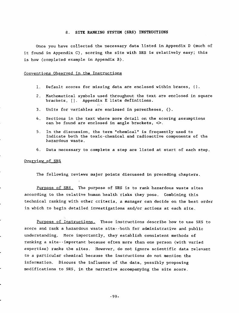
L
8. SITE RANKING SYSTEM (SRS) INSTRUCTIONS
Once you have collected the necessary data listed in Appendix D (much of it found in Appendix C), scoring the site with SRS is relatively easy; this is how (completed example in Appendix B).
Conventions Observed in the Instructions
1. Default scores for missing data are enclosed within braces, 0 .
2. Mathematical symbols used throughout the text are enclosed in square brackets, [ I . Appendix E lists definitions.
3 . Units for variables are enclosed in parentheses, ( ) .
4 . Sections in the text where more detail on the scoring assumptions can be found are enclosed in angle brackets, 0.
5. In the discussion, the term "chemical" is frequently used to indicate both the toxic-chemical and radioactive components of the hazardous waste.
6 . Data necessary to complete a step are listed at start of each step
Overview of SRS
The following reviews major points discussed in preceding chapters.
Purpose of SRS. The purpose of SRS is to rank hazardous waste sites according to the relative human health risks they pose. technical ranking with other criteria, a manager can decide on the best order in which to begin detailed investigations and/or actions at each site.
Combining this
PurDose of Instructions. These instructions describe how to use SRS to score and rank a hazardous waste site--both for administrative and public understanding. More importantly, they establish consistent methods of ranking a site--important because often more than one person (with varied expertise) ranks the sites. However, do not ignore scientific data relevant to a particular chemical because the instructions do not mention the information. Discuss the influence of the data, possibly proposing modifications to SRS, in the narrative accompanying the site score.
-99-

Method of Scoring. SRS ranks sites by scoring important and readily available factors influencing contaminant movement and ultimately human health risk. Although contaminant movement in the environment is complex, SRS simplifies this movement as shown in Figure 8.1 to
three pathways (ground water, surface water, and air)
minimal interaction between these pathways,
direct ingestion or inhalation of the contaminant.
Intricate exposure pathways through food chains are not considered. Furthermore, recycling of contaminants between surface water, ground water, surface soil, and air is assumed a minor component of the ultimate risk.
A
SRS evaluates the relative risk of release [\I along these three release pathways by measuring the potentially exposed population [N], the potential exposure [E] to each waste, and the toxicity [TI for each waste present <Scoring Concept of SRS, Chapter 3>:
a C Nk k R Tlk R - chemical, k - pathway
where Elk is divided further into components of initial waste [W 3 , engineered-barrier-effectiveness factor [f 3 , and site-characteristic factor [fsite] <Chapters 5, 6, and 7 describe the parameters of f
fsite
0
eng and
eng on which scoring is based>
* f a '01 eng,k fsite,lk R - chemical, k = pathway
To simplify the ranking, SRS tabulates scores [F] for the various factors in equations [8.1] and [8.2]. These scores are then combined according to equations [8.1] and [8.2] to obtain the final site score. In SRS, the score for a parameter is the logarithm of that parameter's value <Scoring Individual Factors, Chapter 3>. (Consequently the scores [F] are summed, rather than multiplied to arrive at a composite score.) Because the ranking is not precise, only the logarithm to the nearest integer is used in the tables. Tables ease the use of the ranking system but require specifying parameter units.
- 100 -
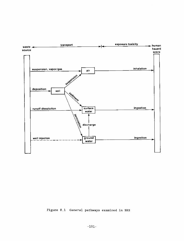
.-
Figure 8 . 1 General pathways examined in SRS
-101-
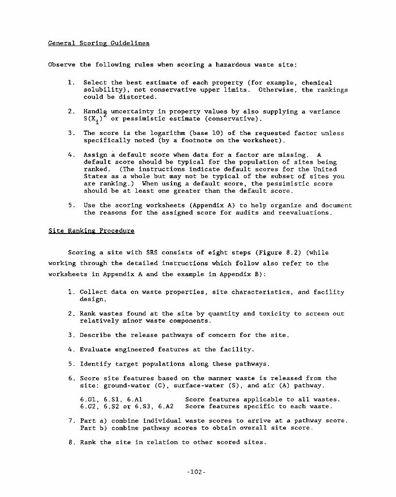
General Scoring Guidelines
Observe the following rules when scoring a hazardous waste site:
1. Select the best estimate of each property (for example, chemical solubility), not conservative upper limits. Otherwise, the rankings could be distorted.
2 . Hand1 uncertainty in property values by also supplying a variance 2 S ( X . ) or pessimistic estimate (conservative). 1
3 . The score is the logarithm (base 10) of the requested factor unless specifically noted (by a footnote on the worksheet).
Assign a default score when data for a factor are missing. default score should be typical for the population of sites being ranked. (The instructions indicate default scores for the United States as a whole but may not be typical of the subset of sites you are ranking.) When using a default score, the pessimistic score should be at least one greater than the default score.
4. A
5. Use the scoring worksheets (Appendix A) to help organize and document the reasons for the assigned score for audits and reevaluations.
Site Ranking Procedure
Scoring a site with SRS consists of eight steps (Figure 8.2) (while working through the detailed instructions which follow also refer to the worksheets in Appendix A and the example in Appendix B):
1. Collect data on waste properties, site characteristics, and facility design.
2. Rank wastes found at the site by quantity and toxicity to screen out relatively minor waste components.
3 . Describe the release pathways of concern for the site.
4 . Evaluate engineered features at the facility.
5. Identify target populations along these pathways.
6. Score site features based on the manner waste is released from the site: ground-water (G), surface-water ( S ) , and air (A) pathway.
6.G1, 6.S1, 6.A1 Score features applicable to all wastes. 6.G2, 6.S2 or 6.S3, 6.A2 Score features specific to each waste.
7. Part a) combine individual waste scores to arrive at a pathway score. Part b) combine pathway scores to obtain overall site score.
8. Rank the site in relation to other scored sites.
- 102 -
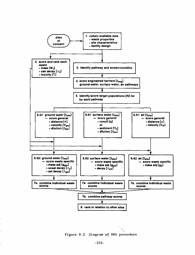
.(-
I
mass [W,] can decay [Ac]
3. identify pathway and screen/combine
toxicity [TI $. 4. score engineered barriers [fen91
ground-water, surface-water, air pathways
+ I I
5. identify/score target populations [N] for for each pathway
I ~ ~~ ~
6.G1 ground water [fritel - score general dlstance [XI velocity [Vgwl dilution [SgWl
I + +
6.S1 surface water [frite] - score general runoff [ql
sediment [Ysl or
dilution [&W]
1 - score general
distance [XI velocity [ V w l
L 6.G2 ground water [fsitel - score waste specific
mass ad1 [agw] unsat decay [A,] sat decay [Agw]
L 6.S2 surface water [frit.] - score waste specific
mass adj [gowl decay [&Wl
6.A2 air [fsit.l - score waste specific mass adj [gal
I 7a. combine individual waste scores
~~ + ~
7a. comblne individual waste scores scores
I 7b. comblne pathway scores I t
8. rank in relation to other sites
‘\ Figure 8.2 Diagram of SRS procedure
-103-
Step 1. Collect data on waste properties, site features, and facility design
The challenging and time-consuming portion of the SRS scheme (or any ranking scheme) is collecting the pertinent data. Each step lists data required (or that you need to estimate) for scoring. (Appendix D repeats this information plus additional unscored data that may help point out unusual features of a particular site.) To help you, Appendix C lists many of the required physical and chemical properties of hazardous waste.
Of all the data collected for SRS, the identity, quantity, and toxicity of waste placed (or to be placed) at a site are the most influential; they determine the maximum potential health risk per exposed individual. Unfortunately, for many abandoned and existing sites, this information is difficult to find. Your tendency may be to rely on site characteristics to mitigate any impact (for example, a slow seepage velocity to greatly reduce the potentially exposed population), but even fairly good sites can become menacing hazards if they contain vast quantities of nondegradable toxic waste and the time frame of interest is long enough; consequently, make a good effort to identify and estimate quantity of the chemical components of the waste. Conceivably, you can still use SRS when you know only the general types of wastes deposited at a site but estimating waste parameters is much more difficult.
Because SRS scores each chemical present along each pathway, the complexity and level of effort to score a site increases with the number of exposure pathways and number of chemicals and radionuclides present. To
avoid collecting unncessary data, keep steps 2 and 3 in mind. These steps identify important chemicals and pathways and screen out the rest.
- 104-
Step 2 . Score and rank chemicals found at site.
Step 2.1: Waste description. First, generally describe the waste at the site (Appendix A), specifically, any major sources of the chemicals (for example, creosote from a tie treatment plant), whether chemicals were concentrated during recovery operations, etc. If less than 6 or 8 chemicals exist at the site, skip to Step 2.3, otherwise continue.
Step 2 . 2 : Enter data on worksheet for screeninp chemicals (Appendix A). The specific data used in this step are
quantity [W ] of each chemical present (kg or Ci) (initial concentratign [C ] times volume times 70 yr) ,
air pathway thought important? ?either AD1 or UCR) ,
0
chronic ingestion toxicity [T ] (and inhalation toxicity [T ] if r l air
3 possibly, solubility [SI (1 kg/m ) .
Chemical quantity. Enter the quantity and score on the worksheet (Appendix A). Score the quantity of waste using Table 8.1. Although the quantity of waste available for release will vary between pathways, neglect
these differences unless they are well known and differ significantly (a factor of 0.3 or less).
Chronic toxicity. Use chronic (long-term) toxicity data [TI, either the allowable daily intake (ADI) or the unit cancer risk (UCR), and enter score (Table 8 . 3 ) on the worksheet. The allowable daily intake (ADI) is defined as the highest human intake of a chemical, expressed in mg/kg/day, that does not cause adverse effects when exposed for a lifetime. The unit cancer risk
(UCR) is the upper lifetime risk per unit of dose, expressed as risk per mg/kg/day <Chronic Toxicity, Chapter 4>. Normally, use toxicity data for a standard cross-section of adults, children, etc. Because chemical toxicity [TI differs for inhalation and ingestion routes, two toxicity scores are needed when the air pathway is significant.
Although in principle the analyst should investigate every chemical present, chemicals with very low toxicity, chemicals with very low mobility, and chemicals that degrade very rapidly may not appreciably affect the overall site risk if in small quantities; consequently, they can be
- 105 -
disregarded. the chemicals according to their hazard as follows:
Therefore, when numerous chemicals are stored at a site, rank
list chemicals found or thought to be at site on preliminary worksheet
If possible group chemicals together to form a class with similar properties.
list quantity [Wo] (or if very difficult to estimate, solubility [SI
record chronic toxicity [TI (UCR or 10 /ADI)
add logartihms of Wo (Table 8 . 1 ) and T (Table 8 . 3 ) (or multiply)
start step 2.3 using chemicals with the larger sums (and any other chemicals you feel especially concerned about)
(Table 8 . 6 ) for each chemical) - 5
Chemicals with scores more than 5 points (5 orders of magnitude) below
the chemical with highest score may not influence the overall risk of the site. The actual score below which to ignore certain chemicals could, however, increase or decrease. Consequently, the cutoff value must be selected on the basis of the first few calculations with the top-ranked chemicals.
With this approach you will concentrate your efforts on hazardous materials more likely to lead to health risks once they escape from the site. Ideally, you will concentrate on no more than 8 chemicals. the chemicals, begin scoring with the main chemical worksheet. [After completing the site scoring, examine the original list for chemicals that may behave similar to those dominating the site score (for example, metals).]
After screening
Step 2 . 3 : Score and rank dominant chemicals. In addition to the data of Step 2.2, this step uses
persistence of chemical while at site, expressed as an average half- life [tl,21 (day)
Chemical half-life. For radioactive wastes, the half-life is a physical property. For toxic metals the half-life is infinite, unless innocuous compounds form. For toxic inorganic or organic compounds, the half-life describes the tendency to degrade into other chemical species, presumably less toxic. The degradation occurs because of hydrolysis,
- 106 -
oxidation, photolysis, and/or biodegradation and is usually specific to the medium <Chemical decay rate, Chapter 5>. Record here the half-life while contained at the site (Table 8.5). Estimates of the average persistence along the specific pathway in various media will be required later. toxicity does not decrease with degradation or the half-life is greater than 10 days (Table 8.6), degradation may not be important.
If
5
On the main chemical worksheet add the scores for the quantity [W ] and 0
toxicity [TI for each chemical. If the chemical can degrade while at the site, add the score (Table 8.5) for the product of half-life [t ] x 6x10-’:
1/2
=. Fmass + Fdecay + Ftox chemical score [ F chem where
- score for chemical quantity = score for chemical decay = score for inhalation or ingestion toxicity
Fmass Fdecay Ftox
After the dominant chemicals have been evaluated, again rank the chemicals according to the chemical risk calculated with T an air pathway).
(or Tair when evaluating oral
Begin scoring the most likely scenario for release (chosen in Step 3 )
using the chemicals with the highest rank (highest potential chemical risk). Completely evaluate the scenario, before starting another. Knowing the dominant chemicals for one scenario will help you evaluate other scenarios.
- 107 -
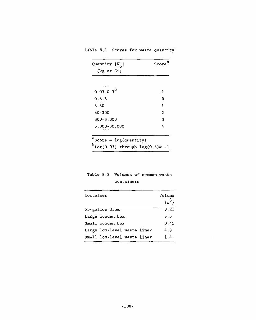
Table 8.1 Scores for waste quantity
Quantity [Wo] Scorea (kg or Ci)
... b 0.03-0.3
0.3-3 3-30 30 - 300 300-3,000 3,000-30,000 . . .
-1 0
4
a
bLog(O .03) through log(O.3)- -1 Score - log(quantity)
Table 8.2 Volumes of common waste containers
Container Volume
(m3 1 55-gallon drum 0.21 Large wooden box 3 . 5
Small wooden box 0.45
Large low-level waste liner 4.8 Small low-level waste liner 1.4
- 108 -
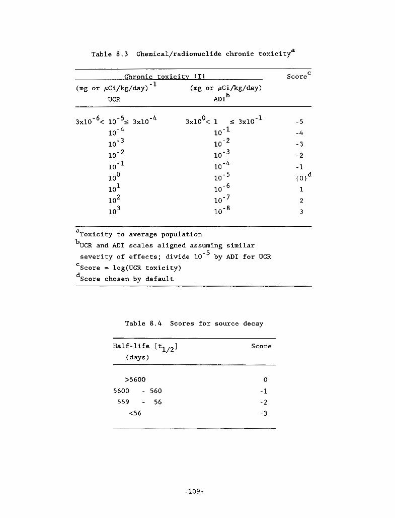
I "
c
c
Table 8.3 Chemical/radionuclide chronic toxicitya
C Chronic toxicity TT1 Score
(mg or pCi/kg/day) (mg or pCi/kg/day) UCR ADIb
-1 3x1Oo< 1 I 3x10 10-1
IO-'
-5 -4 -3 -2 -1 (Old 1 2 3
a
bUCR and AD1 scales aligned assuming similar Toxicity to average population
severity of effects; divide by AD1 for UCR Score = log(UCR toxicity) C
dScore chosen by default
Table 8 . 4 Scores for source decay
Half-life [tlI2]
(days )
Score
>5600 5600 - 560 559 - 56
<5 6
0 -1 -2 -3
- 109 -
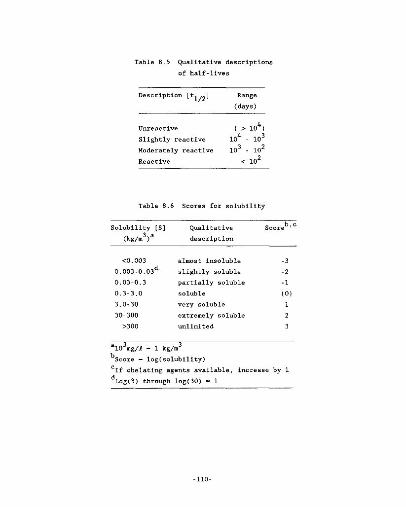
Table 8.5 Qualitative descriptions of half-lives
Range 1/2 1 Description [ t
(days)
Unreactive ( > l o 4 ) Slightly reactive lo4 - IO
Reactive < lo2
3 2 Moderately reactive lo3 - 10
Table 8.6 Scores for solubility
b,c Solubility [SI Qualitative Score (kg/m3 1 a description
<O. 003 almost insoluble -3 0.003-0. 03d slightly soluble - 2
0.03-0.3 partially soluble -1 0.3-3.0 soluble (01
3.0-30 very soluble 1 30 - 300 extremely soluble 2 >300 unl imi t ed 3
a 3 3 10 mg/R = 1 kg/m bScore = log( solubility)
d C If chelating agents available, increase by 1 Log(3) through log(30) = 1
-110-
Step 3. Describe release pathways
Step 3 . 1 : Generallv describe site. First, generally describe the site on the title page of the worksheets (Appendix A).
SteD 3.2: DeveloD and describe Dotential release scenarios. A release scenario is a series of events that could lead to the release of chemicals from the waste site, transport to the environment, and finally damage to the environment or man. Develop and describe these events (Pathways Worksheet, Appendix A) by following the instructions below:
List events or processes that could cause chemical release from the waste source.
L
List processes that could affect transport of the chemical to the environment and the target biologic system.
Combine the events and processes to form scenarios and document them on the pathway worksheet (Appendix A ) . In general, develop all the reasonable scenarios to ensure both yourself and any auditor of the breadth considered. This step identifies for the decision maker the potentially affected targets.
Screen out all but the most probable scenarios and/or combine closely related scenarios into one. are sufficient for this ranking.) easily identify the human population targets of most concern, but unique conditions may require you to reexamine your preliminary decisions after scoring the site. In addition, note but set aside scenarios that ma dyage sensitive environments (defined as areas greater than 2x10 m ) because SRS only ranks human risks. However, have a trained biologist examine the environmental data.
(Probabilities based on your own judgment In general, we presume you will
Group scenarios according to the way in which the released chemical leaves the waste site (air, surface-water, and ground-water pathways) for subsequent scoring.
To clarify the above steps consider the following example. After examining an abandoned waste dump site, you find that several nearby farms withdraw water from an aquifer potentially contaminated by the dump. Only one of these farms uses the aquifer for drinking water; the others use it for livestock. In addition, a distant town withdraws water from this aquifer. One scenario involves release from the site into the aquifer, transport to several farmers’ wells, and then direct consumption. A second scenario
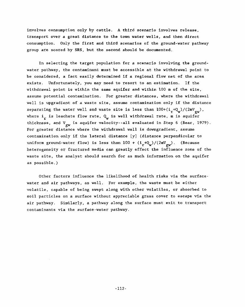
involves consumption only by catcle. A third scenario involves release, transport over a great distance to the town water wells, and then direct consumption. Only the first and third scenarios of the ground-water pathway group are scored by SRS, but the second should be documented.
In selecting the target population for a scenario involving the ground- water pathway, the contaminant must be accessible at the withdrawal point to be considered, a fact easily determined if a regional flow net of the area exists. Unfortunately, you may need to resort to an estimation. If the withdrawal point is within the same aquifer and within 100 m of the site, assume potential contamination. For greater distances, where the withdrawal well is upgradient of a waste site, assume contamination only if the distance separating the water well and waste site is less than 100+(ir+qu)/(2mV where i thickness, and V is aquifer velocity--all evaluated in Step 6 (Bear, 1979). For greater distance where the withdrawal well is downgradient, assume contamination only if the lateral distance [y] (distance perpendicular to uniform ground-water flow) is less than 100 + (ir%)/(2mV heterogeneity or fractured media can greatly effect the influence zone of the waste site, the analyst should search for as much information on the aquifer as possible. )
) , gw is leachate flow rate, Qw is well withdrawal rate, m is aquifer r
gw
) . (Because gw
Other factors influence the likelihood of health risks via the surface- water and air pathways, as well. For example, the waste must be either volatile, capable of being swept along with other volatiles, or absorbed to soil particles on a surface without appreciable grass cover to escape via the air pathway. Similarly, a pathway along the surface must exit to transport contaminants via the surface-water pathway.
-112-
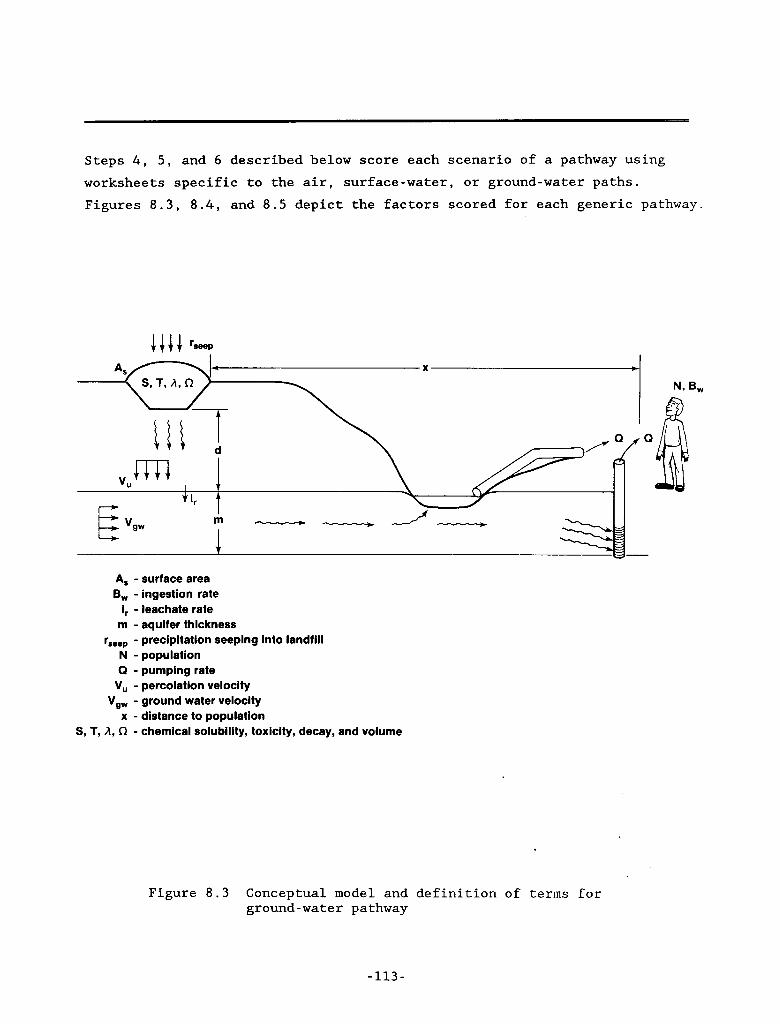
Steps 4 , 5, and 6 described below score each scenario of a pathway using worksheets specific to the air, surface-water, or ground-water paths. Figures 8 . 3 , 8 . 4 , and 8 . 5 depict the factors scored for each generic pathway.
A, - surface area B, - ingestion rate
i, - leachate rate m - aquifer thickness
N - population 0 - pumping rate
Vu - percolatlon velocity Vg, - ground water velocity
x - distance to population
rseep - precipitation seeping into landfill
S, T, A, n - chemical solubility, toxicity, decay, and volume
Figure 8.3 Conceptual model and definition of terms for ground-water pathway
- 113 -
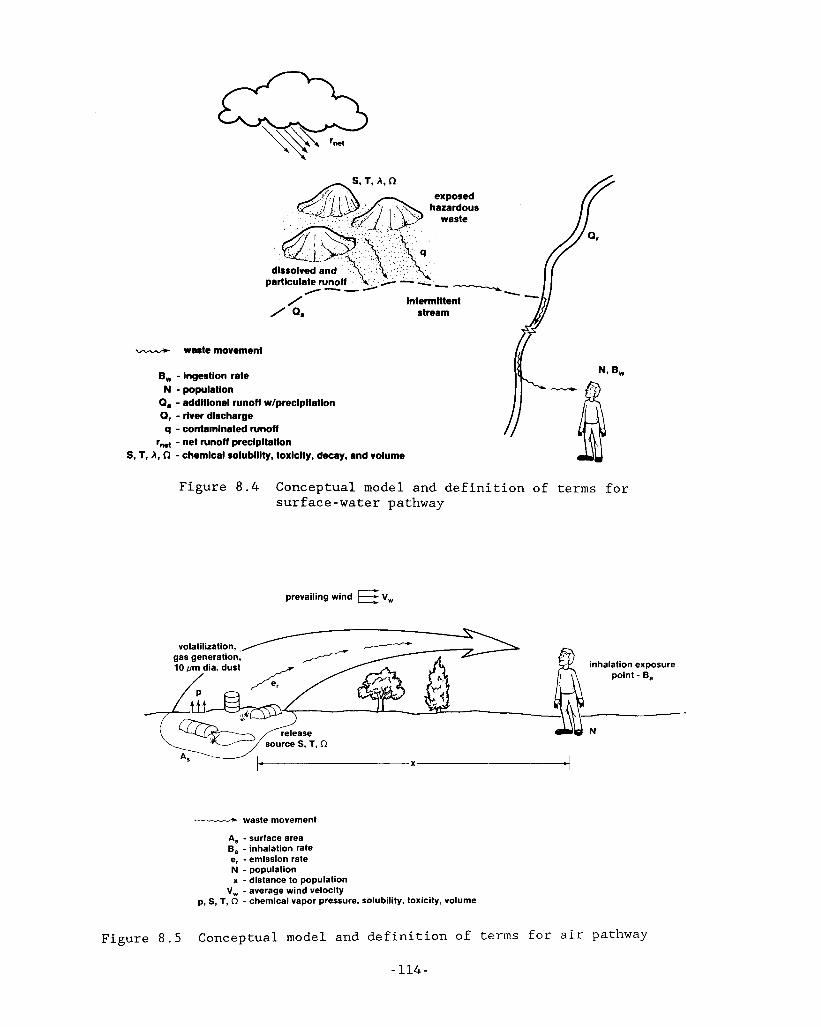
d pa
/ intermittent / Qa stream
waste movement
- ingestion rate - popuiatlon - addltionai runoff w/precipitatlon - river dlscharge - contamlnated runoff - net runoff precipitation - chemical solubility, toxlclty, decay, and volume
Figure 8.4 Conceptual model and definition of terms for surface-water pathway
prevailing wind E v,
volatilization, -------
/
aas aeneration.
P
source S, T, fl
a x -
___t waste movement
A, - surface area 6, - inhalation rate e, - emission rate N - population x - distance to population
V, - average wind velocity p, S, T, fl - chemical vapor pressure, solubility, toxicity, volume
inhalation exposure point - B,
N
Figure 8.5 Conceptual model and definition of terms for air pathway
-114-
Step 4 . Evaluate engineered barriers at site
Engineered barriers serve to
1. extend containment of the chemical (beneficial if decay occurs),
2 . lower the release rate, and
3 . minimize access to the chemical.
They do not, however, always provide indefinite isolation, especially for nondegradable waste contaminating ground-water. Under topic 1, "extend containment of the chemical," individual container life was evaluated with the chemical hazard, Step 1. Under topic 3 , "minimize access to the chemical," waste covers and liners are evaluated along with leachate and gas generation, Step 6 . The topics evaluated here are primarily concerned with barriers that lower the release rate of the chemical.
Usually, scores for the engineered barriers will apply to all pathways in a group (for example, the ground-water route) and, thus, reduce the evaluation effort. This grouping was assumed in the design of the worksheets (Appendix A). This grouping is not universal, however, and barriers could be very specific to a particular chemical waste. Furthermore, a waste facility could involve several disposal methods. In this latter case, consider scoring each disposal method individually and combining scores to determine an overall facility score using the combination scheme described in Step 7.
SteD 4 . 1 : TvDe of storage. The probability of failure based on the type of storage is partially accounted for in this step. For example, haphazard disposal on vacant property would most likely lead to contamination by any pathway; storage of liquid wastes in lagoons would rate next, landfills of questionable design next; and well-designed or specially constructed landfills would presumably provide the lowest risk. In other words, although engineered containment intact today may fail later, current risks are greater when the containment is poor. Furthermore, good containment today provides more time for a permanent solution. Consequently, a small weighting is used to penalize sites with poor waste placement. The
- 115 -
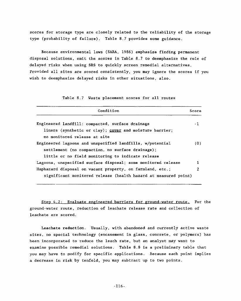
scores for storage type are closely related to the reliability of the storage type (probability of failure). Table 8 . 7 provides some guidance.
Because environmental laws (SARA, 1986) emphasize finding permanent disposal solutions, omit the scores in Table 8.7 to deemphasize the role of delayed risks when using SRS to quickly screen remedial alternatives. Provided all sites are scored consistently, you may ignore the scores if you wish to deemphasize delayed risks in other situations, also.
Table 8 . 7 Waste placement scores for all routes
Condition Score
Engineered landfill: compacted, surface drainage -1 liners (synthetic or clay); cover and moisture barrier; no monitored release at site
Engineered lagoons and unspecified landfills, w/potential (0) settlement (no compaction, no surface drainage); little or no field monitoring to indicate release
Lagoons, unspecified surface disposal; some monitored release 1 Haphazard disposal on vacant property, on farmland, etc.; 2
significant monitored release (health hazard at measured point)
SteD 4 . 2 : Evaluate enpineered - barriers for eround-water route. For the ground-water route, reduction of leachate release rate and collection of leachate are scored.
Leachate reduction. Usually, with abandoned and currently active waste sites, no special technology (encasement in glass, concrete, or polymers) has been incorporated to reduce the leach rate, but an analyst may want to examine possible remedial solutions. Table 8 . 8 is a preliminary table that you may have to modify for specific applications. a decrease in risk by tenfold, you may subtract up to two points.
Because each point implies

Table 8.8 Leachate reduction for ground-water route
~
Condition Score
No special treatment (01 Concrete encasement -1 Synthetic organic polymers - 2
Leachate collection system. A leachate collection system can reduce the risk of release (Table 8.9). not last 70 yr (average life expectancy), a leachate system operated for many years can remove a substantial percentage of the waste since concentration of the leachate decreases exponentially if no additional material is added. Consequently, a good site might include synthetic liners and a leachate collection system for reducing the chemical hazard for the first few years plus a clay cover to reduce infiltration over the long term.
Even though a leachate collection system will
Table 8.9 Leachate collection system for ground water route
Condition Score
None (01
Collection with treatment -1
Step 4 . 3 : Evaluate engineered barriers for surface-water route. Evaluate the hydraulic drainage structures around the site and the depth of soil cover using Table 8.10. If no structures exist or surface-water pathway is unimportant, skip to Step 4.4 .
The use of drainage facilities and 1 or 2 m of soil cover [ S I can significantly reduce the possibility of release of toxic chemicals via the surface-water pathway; however, flooding may greatly increase the possibility
-117-
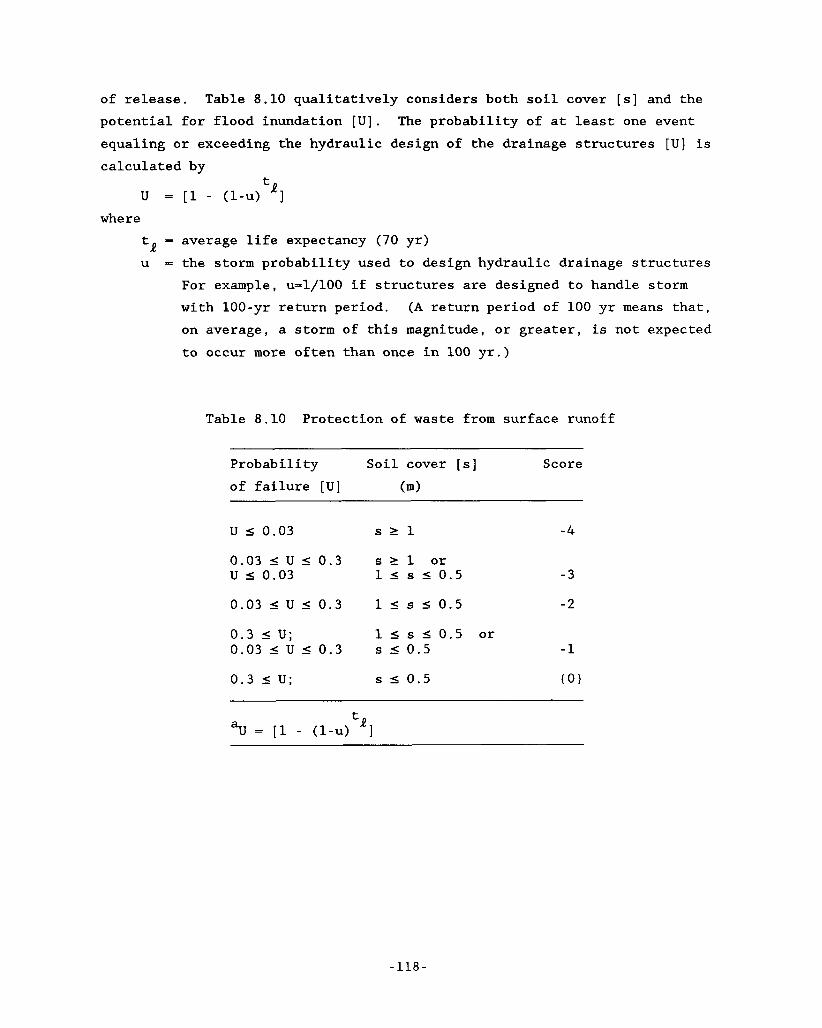
of release. Table 8.10 qualitatively considers both soil cover [ S I and the potential for flood inundation [ U ] . The probability of at least one event equaling or exceeding the hydraulic design of the drainage structures [U] is calculated by
u = [l - (1-u) 3 where
tR = average life expectancy (70 yr) u - the storm probability used to design hydraulic drainage structures
For example, u-1/100 if structures are designed to handle storm with 100-yr return period. (A return period of 100 yr means that, on average, a storm of this magnitude, or greater, is not expected to occur more often than once in 100 yr.)
Table 8.10 Protection of waste from surface runoff
Probability Soil cover [ S I Score
of failure [ U ] (m)
u I 0.03 S l l -4
0.03 5 U I 0 . 3 s l l or u I 0.03 1 I s I 0.5 - 3
0.03 5 U 5 0 . 3 1 I s 5 0 . 5 - 2
0 . 3 I U; 1 I s I 0 . 5 or 0.03 < U 1 0 . 3 s s 0 . 5 -1
0 . 3 I U ; s 5 0 . 5 (0)
“v - [l - (1-u) ]
-118-
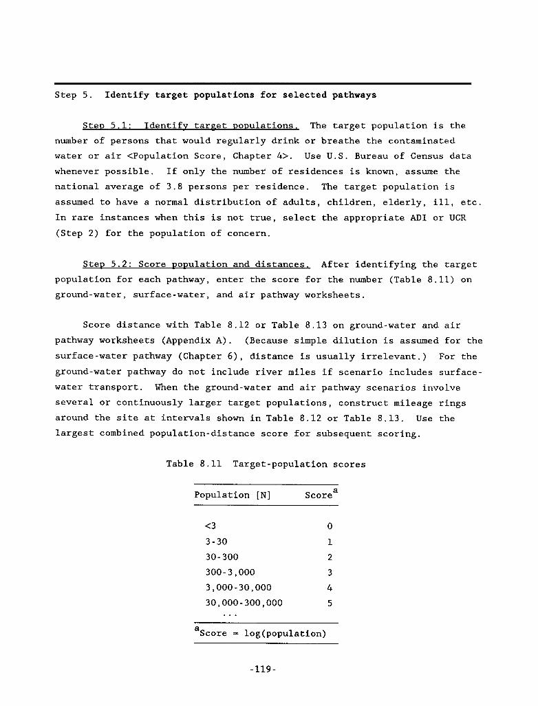
Step 5. Identify target populations for selected pathways
Step 5.1: Identifv target populations. The target population is the number of persons that would regularly drink or breathe the contaminated water or air <Population Score, Chapter 4>. Use U.S. Bureau of Census data whenever possible. If only the number of residences is known, assume the national average of 3.8 persons per residence. The target population is assumed to have a normal distribution of adults, children, elderly, ill, etc. In rare instances when this is not true, select the appropriate AD1 or UCR (Step 2) for the population of concern.
Step 5.2: Score population and distances. After identifying the target population for each pathway, enter the score for the number (Table 8.11) on ground-water, surface-water, and air pathway worksheets.
Score distance with Table 8.12 or Table 8.13 on ground-water and air pathway worksheets (Appendix A). surface-water pathway (Chapter 6 ) , distance is usually irrelevant.) For the ground-water pathway do not include river miles if scenario includes surface- water transport. When the ground-water and air pathway scenarios involve several or continuously larger target populations, construct mileage rings around the site at intervals shown in Table 8.12 or Table 8.13. Use the largest combined population-distance score for subsequent scoring.
(Because simple dilution is assumed for the
Table 8.11 Target-population scores
Population [N] Scorea
<3 0
3-30 1 30 - 300 2 300-3,000 3 3,000-30,000 4 30,000-300,000 5
. . . a Score - log(popu1ation)
- 119 -
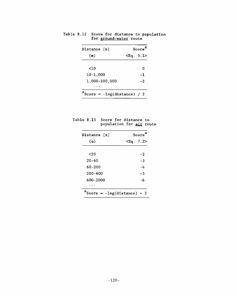
Table 8.12 Score for distance to population for ground-water route
a
(m) <Eq. 5.1> Distance [ X I Score
4 0 0
10-1,000 -1 1,000-100,000 - 2
. . . a Score - -log(distance) / 2
Table 8.13 Score for distance to population for route
a
(m) <Eq. 7.2> Distance [ X I Score
<20
20-60 60- 200
200 - 600
600 - 2000 . . .
-2 - 3
-4
- 5
-6
a Score = -log(distance) 2
- 120 -
Step 6. Score site features based on way in which waste is released
The following instructions for scoring site features are specific to the way in which the waste leaves the site (via air, surface water, or ground water). those for the surface-water route, 6.Sx; and those for the air route, 6 . h .
The steps applicable to the ground-water route are designated 6.Gx;
6.G1, 6.S1, 6.A1 Score features applicable to all wastes. 6.G2, 6.S2 or 6.S3, 6.A2 Score features specific to each waste.
For Step 6, completely score one scenario, and then all scenarios in a pathway before moving on to a scenario in another pathway.
-121-
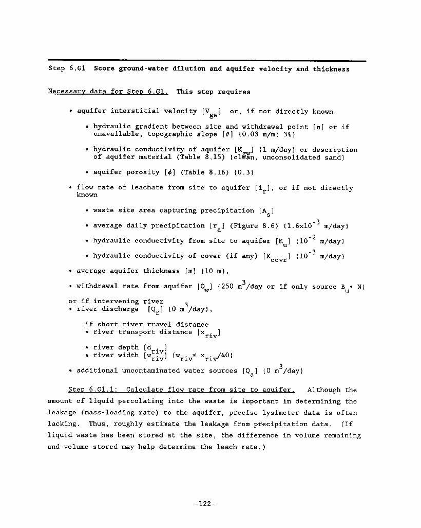
Step 6.G1 Score ground-water dilution and aquifer velocity and thickness
Necessarv data for SteD 6.G1. This step requires
aquifer interstitial velocity [V ] or, if not directly known gw
hydraulic gradient between site and withdrawal point [ q ] or if unavailable, topographic slope [ e ] (0.03 m/m; 3 % )
hydraulic conductivity of aquifer [K ] (1 m/day) or description of aquifer material (Table 8.15) (clEn, unconsolidated sand)
aquifer porosity [ d ] (Table 8.16) (0.3)
flow rate of leachate from site to aquifer [i,], or if not directly known
waste site area capturing precipitation [ A ] S
average daily precipitation [r ] (Figure 8.6) (1.6~10 - 3 m/day) a
hydraulic conductivity from site to aquifer [Ku] m/day)
hydraulic conductivity of cover (if any) [K ] m/day) covr average aquifer thickness [m] (10 m ) ,
3 withdrawal rate from aquifer [QJ (250 m /day or if only source B N)
or if intervening river river discharge [Q,] ( 0 m /day),
U
3
if short river travel distance river transport distance [x ] r iv river depth [driv] river width [wriv] (writ x / 4 0 ) r iv
3 additional uncontaminated water sources [Q,] (0 m /day)
SteD 6.Gl.l: Calculate flow rate from site to aauifer. Although the amount of liquid percolating into the waste is important in determining the leakage (mass-loading rate) to the aquifer, precise lysimeter data is often lacking. Thus, roughly estimate the leakage from precipitation data. (If liquid waste has been stored at the site, the difference in volume remaining and volume stored may help determine the leach rate.)
- 1 2 2 -
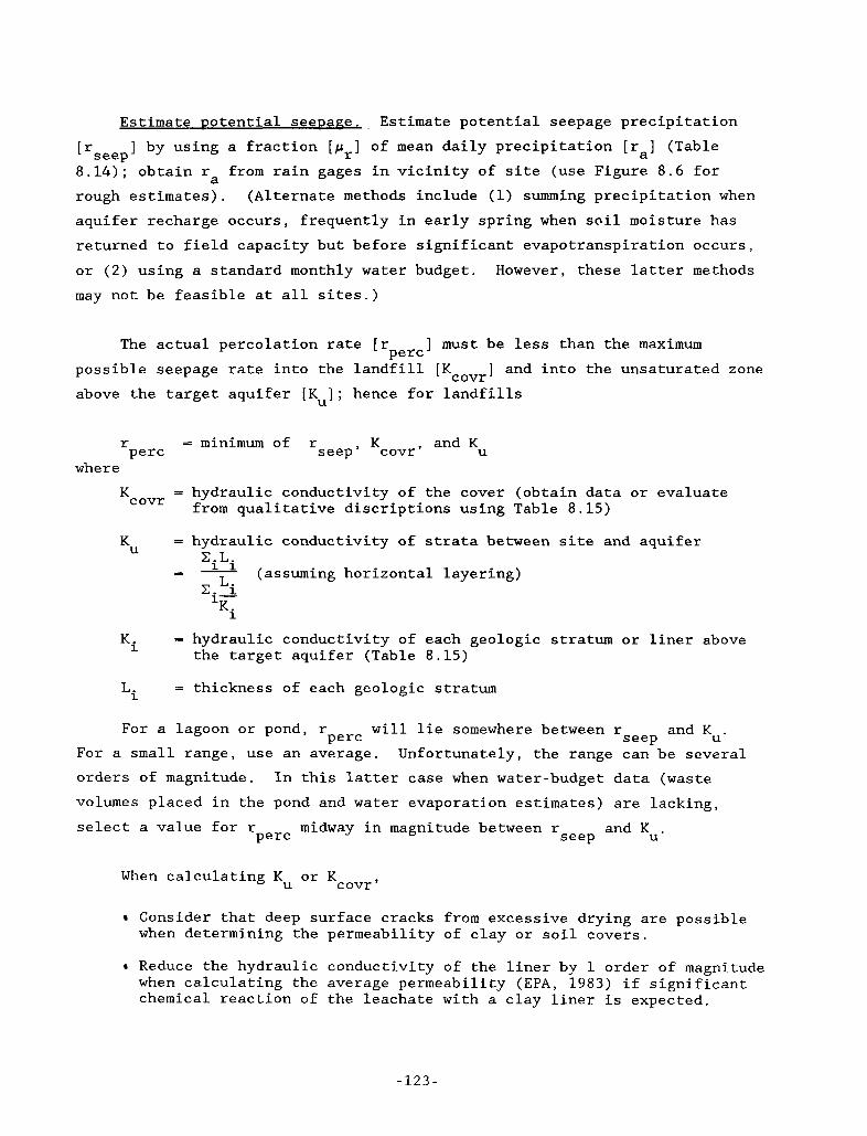
c
Estimate potential seepage. Estimate potential seepage precipitation ] by using a fraction [pr] of mean daily precipitation [r,] (Table [rseep
8.14); obtain ra from rain gages in vicinity of site (use Figure 8.6 for rough estimates). (Alternate methods include (1) summing precipitation when aquifer recharge occurs, frequently in early spring when soil moisture has returned to field capacity but before significant evapotranspiration occurs, or (2) using a standard monthly water budget. However, these latter methods may not be feasible at all sites.)
The actual percolation rate [r ] must be less than the maximum perc possible seepage rate into the landfill [K ] and into the unsaturated zone above the target aquifer [K 1 ; hence for landfills
covr U
r perc where
= minimum of and K seep' Kcovr' U r
hydraulic conductivity of the cover (obtain data or evaluate from qualitative discriptions using Table 8.15)
hydraulic conductivity of strata between site and aquifer
(assuming horizontal layering) XiLi
X. i Ki
L 1-
hydraulic conductivity of each geologic stratum or liner above the target aquifer (Table 8.15)
thickness of each geologic stratum
For a lagoon or pond, r perc will lie somewhere between rseep and KU. For a small range, use an average. Unfortunately, the range can be several orders of magnitude. In this latter case when water-budget data (waste volumes placed in the pond and water evaporation estimates) are lacking, select a value for rperc midway in magnitude between r and KU. seep
When calculating K or KcOvr, U
Consider that deep surface cracks from excessive drying are possible when determining the permeability of clay or soil covers.
Reduce the hydraulic conductivity of the liner by 1 order of magnitude when calculating the average permeability (EPA, 1983) if significant chemical reaction of the leachate with a clay liner is expected.
- 1 2 3 -
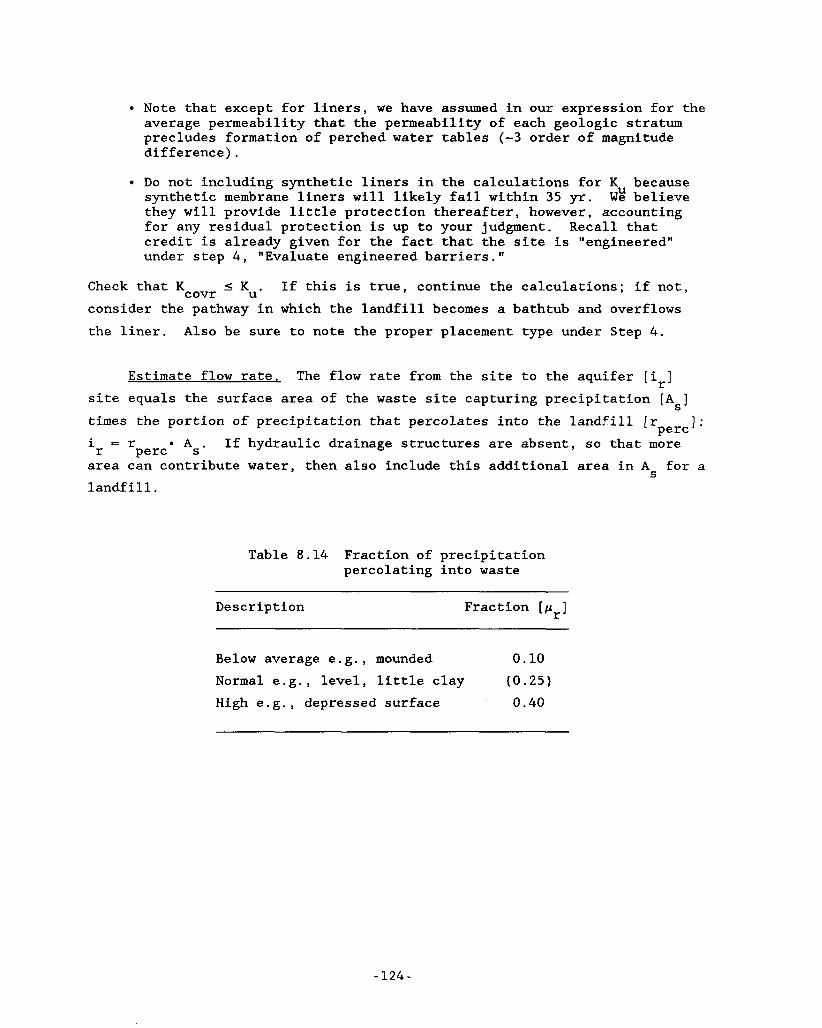
Note that except for liners, we have assumed in our expression for the average permeability that the permeability of each geologic stratum precludes formation of perched water tables (-3 order of magnitude difference).
Do not including synthetic liners in the calculations for Ku because synthetic membrane liners will likely fail within 35 yr. We believe they will provide little protection thereafter, however, accounting for any residual protection is up to your judgment. Recall that credit is already given for the fact that the site is "engineered" under step 4 , "Evaluate engineered barriers."
Check that Kcovr I Ku. consider the pathway in which the landfill becomes a bathtub and overflows the liner. Also be sure to note the proper placement type under Step 4 .
If this is true, continue the calculations; if not,
Estimate flow rate. The flow rate from the site to the aquifer [i,] site equals the surface area of the waste site capturing precipitation [ A ]
times the portion of precipitation that percolates into the landfill [rperc]: i = r . If hydraulic drainage structures are absent, so that more area can contribute water, then also include this additional area in As for a landfill.
S
r perc. As
Table 8.14 Fraction of precipitation percolating into waste
Description Fraction [p,]
Below average e.g., mounded 0.10 Normal e.g., level, little clay (0 .25 )
High e.g., depressed surface 0.40
- 124-
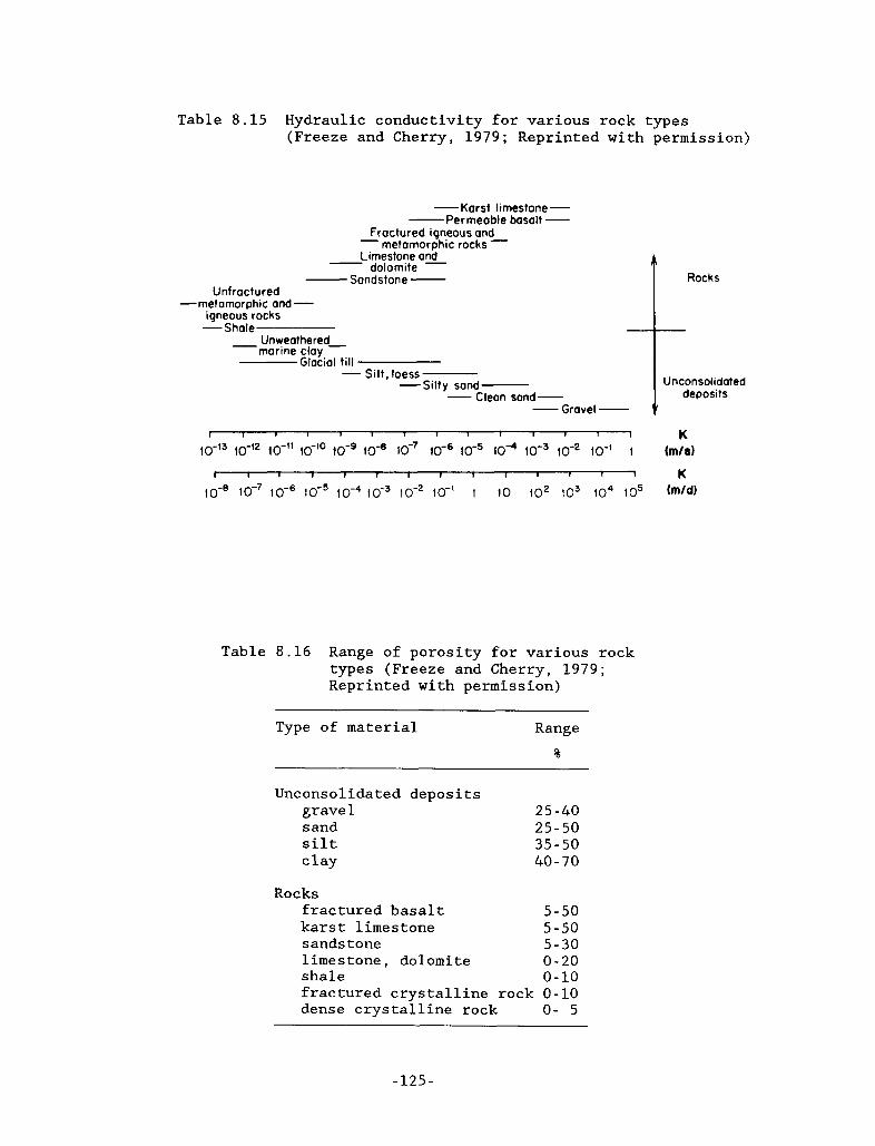
Table 8 . 1 5 Hydraulic conductivity for various rock types (Freeze and Cherry, 1979; Reprinted with permission)
Karst limestone - -Permeable basalt - -
- Fractured igneous and- metamorphic rocks
Limestone a&
Sandstone - - dolomite
Unfractured -metamorphic and-
igneous rocks -Shale - Unweathered-
marine clay Glacial till
Rocks
Unconsolidated deposits
Gravel -
- Silt, loess -Silty sand- - Clean sand- -
t 1 1 I 1 1 1 I K 10-13 10-12 10-11 10-10 10” lo-’ lo-’ lo-* lo-‘ 1 (fill61
t I 1 I 1 I 1 I I 1 I 1 1 1 K
Table 8.16 Range of porosity for various rock types (Freeze and Cherry, 1979; Reprinted with permission)
Type of material Range %
Unconsolidated deposits gravel 2 5 - 4 0 sand 25 - 50 silt 35 - 50 clay 40 - 70
Rocks fractured basalt 5 - 5 0 karst limestone 5 - 5 0 sands tone 5 - 3 0 limestone, dolomite 0 - 2 0 shale 0-10 fractured crystalline rock 0-10 dense crystalline rock 0- 5
- 1 2 5 -
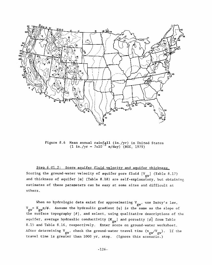
Figure 8.6 Mean annual rainf 11 (in./yr) in United States -3 (1 in./yr = 7x10 m/day) (NCC, 1979)
Step 6.G1.2: Score aquifer fluid velocity and aquifer thickness. Scoring the ground-water velocity of aquifer pore fluid [V and thickness of aquifer [m] (Table 8.18) are self-explanatory, but obtaining estimates of these parameters can be easy at some sites and difficult at
] (Table 8.17) gw
others.
When no hydrologic data exist for approximating V use Darcy’s law, gw’
Vgw= Kgwq/4. the surface topography [ e ] , and select, using qualitative descriptions of the aquifer, average hydraulic conductivity [K 8.15 and Table 8.16, respectively. Enter score on ground-water worksheet. After determining V check the ground-water travel time (x /V ) . If the travel time is greater than 1000 yr, stop.
Assume the hydraulic gradient [ q ] is the same as the slope of
] and porosity [q51 from Table gw
gw ’ gw gw (Ignore this scenario.)
-126-
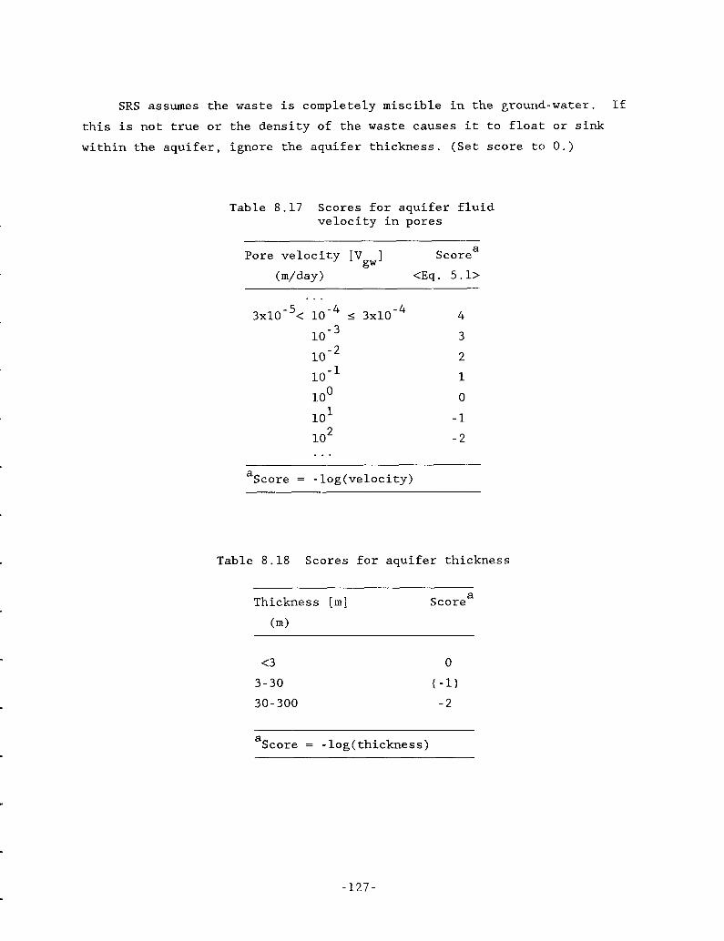
I-
P
SRS assumes the waste is completely miscible in the ground-water. If this is not true or the density of the waste causes it to float or sink within the aquifer, ignore the aquifer thickness. (Set score to 0.)
Table 8.17 Scores for aquifer fluid velocity in pores
a
(m/day) <Eq. 5 .1> Pore velocity [V ] Score
gw
. . . 4
3 2
- 4 3 ~ 1 0 - ~ < I 3x10
10-1 1
l o o 0
lo1 -1 l o 2 - 2 . . .
a Score = -log(velocity)
Table 8.18 Scores for aquifer thickness
a Thickness [m] Score
(m)
<3 3-30
30- 300
0
(-1) - 2
a Score = -log(thickness)
- 127 -
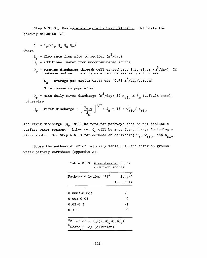
Step 6.G1.3: Evaluate and score pathway dilution. Calculate the pathway dilution [SI:
6 = where
i = r
Qa =
Q w =
Qr =
otherwise
3 flow rate from site to aquifer (m /day) additional water from uncontaminated source
3 pumping discharge through well or recharge into river (m /day) If unknown and well is only water source assume B N where
U
B =
N =
mean
U 3 average per capita water use (0 .76 m /day/person)
community population
daily river discharge (m /day) if xriv 2 Rm (default case); 3
1/2 2 Qr = river discharge [ x;iv ] ; R m = 15 Wriv/ driv m
The river discharge [Q,] will be zero for pathways that do not include a surface-water segment. river route.
Likewise, Qw will be zero for pathways including a See Step 6.S1.5 for methods on estimating Qr, w and driv. riv’
Score the pathway dilution [6] using Table 8.19 and enter on ground- water pathway worksheet (Appendix A).
Table 8 . 1 9 Ground-water route dilution scores
b Pathway dilution [ 6 J a Score < E q . 5.1>
. . . 0.0003-0.003 0.003-0.03 0.03-0.3 0.3-1
-3 -2 -1 0
Dilution = i /(i +Qw+Q +Q ) a
bScore = l og (dilution) r r r a
- 128 -
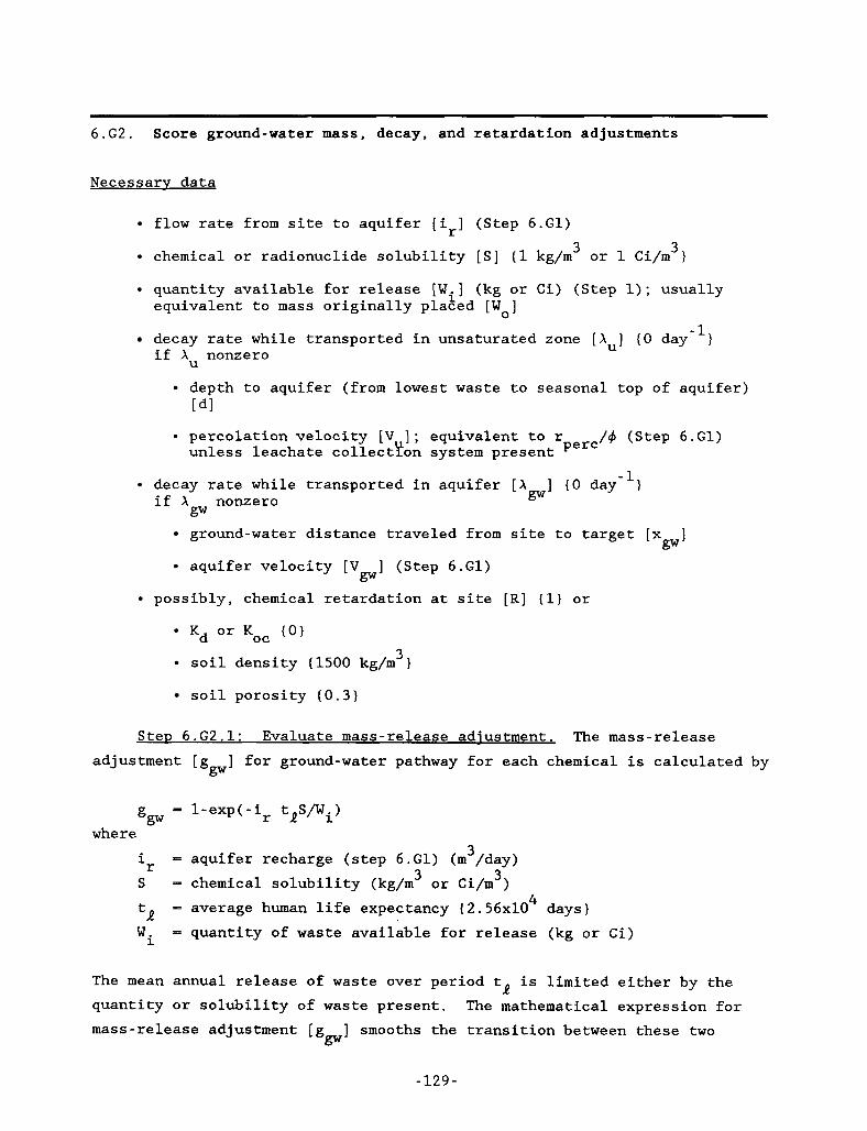
6.G2. Score ground-water mass, decay, and retardation adjustments
Necessarv data
flow rate from site to aquifer [i,] (Step 6.G1)
chemical or radionuclide solubility [SI (1 kg/m3 or 1 Ci/m ) 3
quantity available for release [Wi] (kg or Ci) (Step 1); usually equivalent to mass originally placed [W 3
0 -1 decay rate while transported in unsaturated zone [ X u ] (0 day )
if Xu nonzero
depth to aquifer (from lowest waste to seasonal top of aquifer) dl
9 percolation velocity [V 1 ; equivalent to r /c$ (Step 6.G1) U perc unless leachate collection system present
decay rate while transported in aquifer [ A ] (0 day-') gw if X nonzero gw ground-water distance traveled from site to target [x ]
aquifer velocity [V ] (Step 6.G1) gw
gw possibly, chemical retardation at site [R] (1) or
Kd Or Koc (0) 3 soil density (1500 kg/m )
soil porosity ( 0 . 3 )
SteD 6.G2.1: Evaluate mass-release adjustment. The mass-release adjustment [g ] for ground-water pathway for each chemical is calculated by
gw
= 1-exp(-i tRS/Wi) ggw r
i - aquifer recharge (step 6.G1) (m /day) S - chemical solubility (kg/m or Ci/m )
tR - average human life expectancy (2.56~10 days) 'i
where 3
3 3 r
4
- quantity of waste available for release (kg or Ci) The mean annual release of waste over period t quantity or solubility of waste present. mass-release adjustment [g ] smooths the transition between these two
is limited either by the R The mathematical expression for
gw
- 129 -
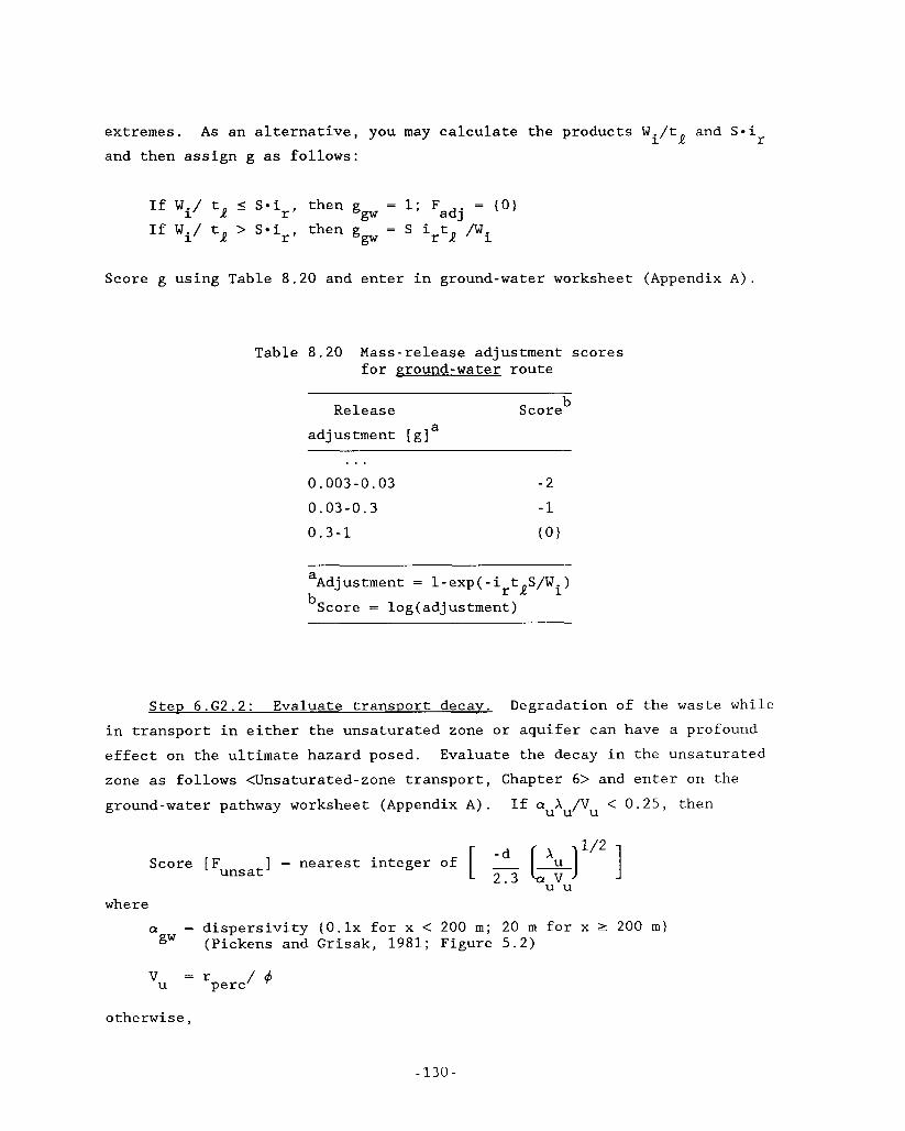
extremes. and then assign g as follows:
As an alternative, you may calculate the products W./t and S-i, 1 l
If W./ t, I Seir, then g = 1; Fadj = ( 0 ) 1 gw
gw If Wi/ tl > Seir, then g = S i,t, /Wi
Score g using Table 8.20 and enter in ground-water worksheet (Appendix A ) .
Table 8.20 Mass-release adjustment scores for ground-water route
b Release Score a adjustment [ g ]
. . . 0.003-0.03 0.03-0.3 0.3-1
-2 -1 ( 0 )
a
bScore = log(adjustment) Adjustment = 1-exp(-i r l t S/W.) 1
Stev 6.G2.2: Evaluate transport decay. Degradation o f the waste while in transport in either the unsaturated zone or aquifer can have a profound effect on the ultimate hazard posed. zone as follows <Unsaturated-zone transport, Chapter 6> and enter on the ground-water pathway worksheet (Appendix A).
Evaluate the decay in the unsaturated
If aUXU/VU < 0.25, then
where CY = dispersivity (0.1~ for x < 200 m ; 20 m for x 2 200 m ) gw (Pickens and Grisak, 1981; Figure 5.2)
otherwise,
-130-
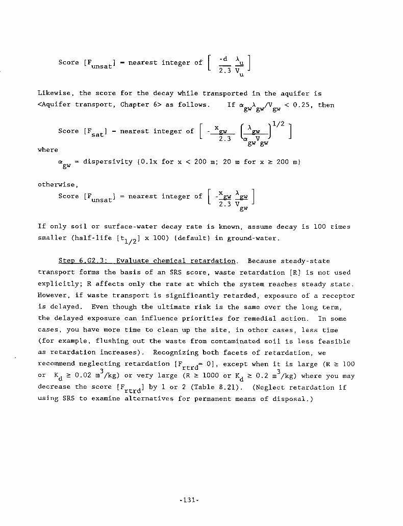
Score [ F ~ ~ ~ ~ ~ I = nearest integer of [ -d xu ] 2.3 Vu
Likewise, the score for the decay while transported in the aquifer is aquifer transport, Chapter 6> as follows. If a x < 0.25, then
gw gw/vgw
1/2 [ -* p.;: 1 1 Score [Fsat] = nearest integer of
gw gw where
a = dispersivity ( 0 . 1 ~ for x < 200 m; 20 m for x 1 2 0 0 m) gw
otherwise, Score [ F ~ ~ ~ ~ ~ I = nearest integer of [ -% e] x
2.3 V gw
If only soil or surface-water decay rate is known, assume decay is 100 times smaller (half-life [t ] x 100) (default) in ground-water. 1/2
Step 6.G2.3: Evaluate chemical retardation. Because steady-state transport forms the basis of an SRS score, waste retardation [R] is not used explicitly; R affects only the rate at which the system reaches steady state. However, if waste transport is significantly retarded, exposure of a receptor is delayed. Even though the ultimate risk is the same over the long term,
*- the delayed exposure can influence priorities for remedial action. cases, you have more time to clean up the site, in other cases, less time
In some
- (for example, flushing out the waste from contaminated soil is less feasible as retardation increases). Recognizing both facets of retardation, we
recommend neglecting retardation [F rtrd= 01, except when it is large (R 1 100 3 3 or > 0.2 m /kg) where you may
decrease the score [F ] by 1 or 2 (Table 8.21). (Neglect retardation if using SRS to examine alternatives for permanent means of disposal.)
.- Kd 10.02 m /kg) or very large (R 11000 or K d -
rtrd -
.-
e
.-
e -131-
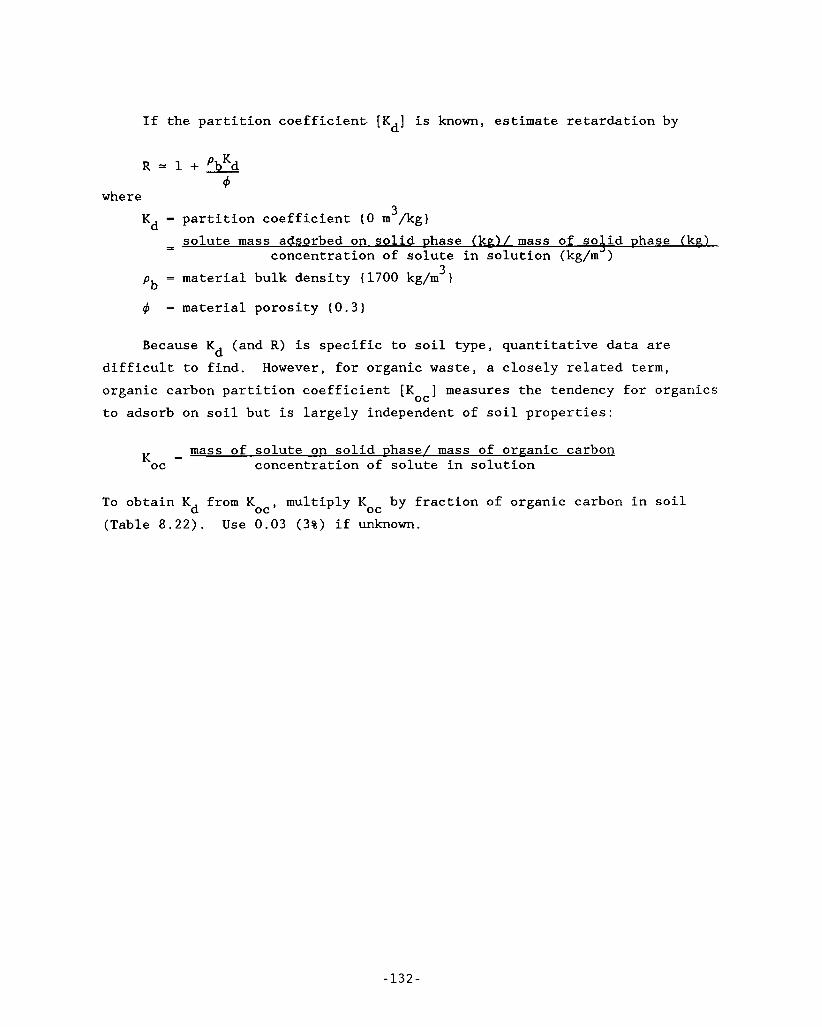
If the partition coefficient. [Kd] is known, estimate retardation by
R = 1 + 'bKd 4
where 3 K = partition coefficient (0 m /kg) d
solute mass adsorbed on solid Dhase (kF)/ mass of solid phase (kg) concentration of solute in solution (kg/m-')
3
= -
= material bulk density (1700 kg/m 1 'b 4 - material porosity (0.3) Because K (and R) is specific to s o i l type, quantitative data are
difficult to find. However, for organic waste, a closely related term, organic carbon partition coefficient [K ] measures the tendency for organics to adsorb on soil but is largely independent of soil properties:
d
oc
mass of solute on solid phase/ mass of organic - carbon Koc = concentration of solute in solution
To obtain Kd from KoC, multiply Koc by fraction of organic carbon in soil (Table 8.22). Use 0.03 ( 3 % ) if unknown.
- 132 -
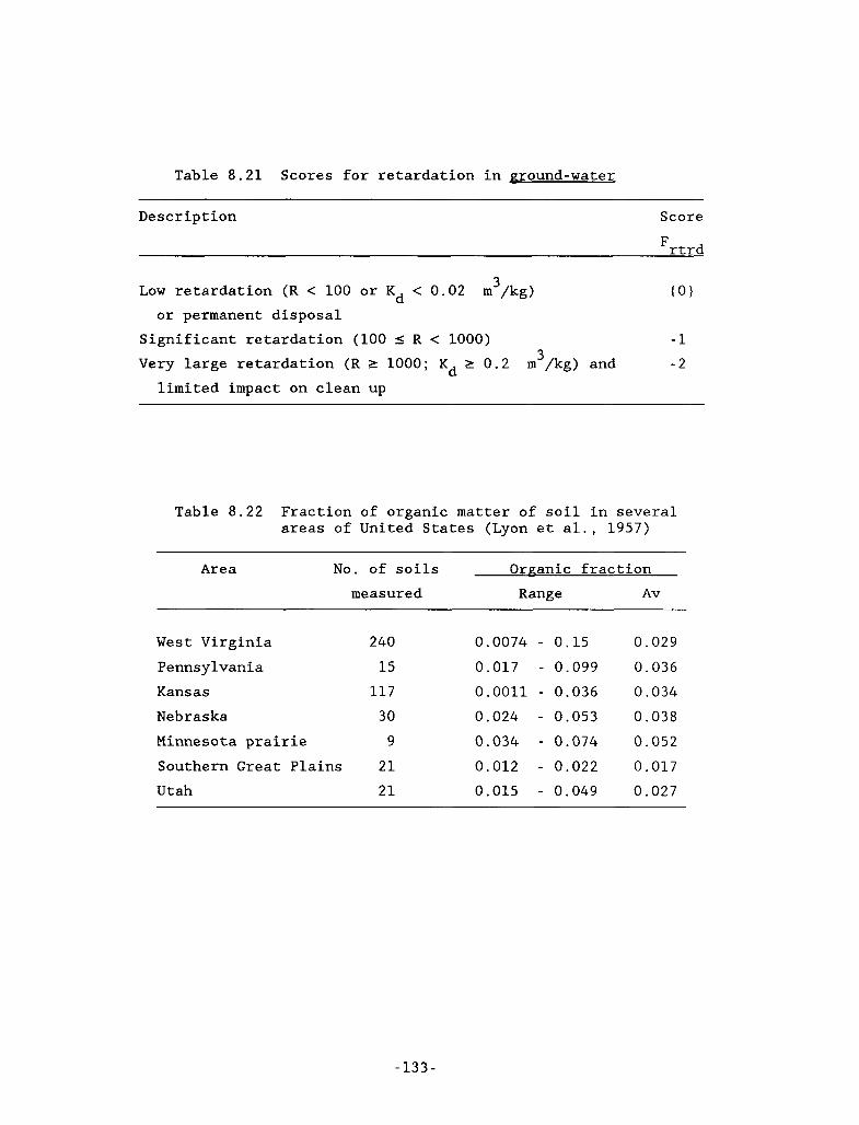
.-
Table 8 . 2 1 Scores for retardation in ground-water
Description Score
Frtrd
( 0 ) 3 Low retardation (R < 100 or Kd < 0.02 m /kg)
or permanent disposal Significant retardation (100 I R < 1000) -1
- 2 3 Very large retardation (R 2 1000; Kd 2 0.2 m /kg) and limited impact on clean up
Table 8 . 2 2 Fraction of organic matter of soil in several areas of United States (Lyon et al., 1 9 5 7 )
Area No. of soils Organic fraction measured Range Av
West Virginia 240 0 . 0 0 7 4 - 0 . 1 5 0 . 0 2 9
Pennsylvania 1 5 0 . 0 1 7 - 0 . 0 9 9 0 . 0 3 6
Kansas 117 0.0011 - 0 . 0 3 6 0 . 0 3 4
0 . 0 3 8 Nebraska 30 0 . 0 2 4 - 0 . 0 5 3
Minnesota prairie 9 0 . 0 3 4 - 0 . 0 7 4 0 .052
Southern Great Plains 2 1 0 . 0 1 2 - 0 . 0 2 2 0 . 0 1 7
Utah 21 0 . 0 1 5 - 0 . 0 4 9 0 . 0 2 7
- 1 3 3 -
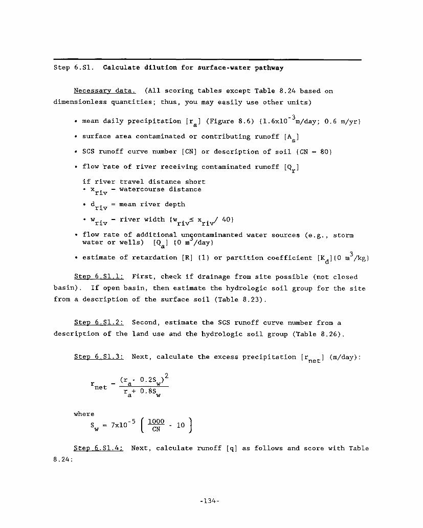
Step 6.S1. Calculate dilution for surface-water pathway
Necessarv data. (All scoring tables except Table 8.24 based on dimensionless quantities; thus, you may easily use other units)
mean daily precipitation Ira] (Figure 8.6) ( 1.6~10-~m/day; 0.6 m/yr)
surface area contaminated or contributing runoff [A 3 SCS runoff curve number [CN] or description of soil (CN = 80)
S
flow 'rate of river receiving contaminated runoff [Q ] r if river travel distance short * x = watercourse distance r iv
driv - mean river depth * w = river width (wrivS xriJ 40) r iv flow rate of additional un ontaminanted water sources (e.g., storm 5 water or wells) [Q,] (0 m /day)
estimate of retardation [R] (1) or partition coefficient [Kd](O m 3 /kg)
Step 6.Sl.l: First, check if drainage from site possible (not closed basin). from a description of the surface soil (Table 8.23).
If open basin, then estimate the hydrologic soil group for the site
Step 6.S1.2: Second, estimate the SCS runoff curve number from a description of the land use and the hydrologic soil group (Table 8.26).
Step 6.S1.3: Next, calculate the excess precipitation [r ] (m/day): net
(ra- 0.2Sw) 2 - - r
net ra+ 0.8Sw
where sW = ~ X I O - ~ [ - i o ]
Step 6.S1.4: Next, calculate runoff [q] as follows and score with Table
8.24:
-134-
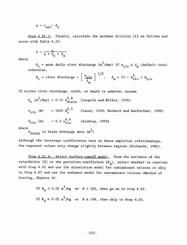
net. As q = r
,-
e
-
.-
Step 6.S1.5 : Finally, calculate the pathway dilution [SI as follows and score with Table 8.25 :
S = 4 q + Qr + Qa
where 3 Qr = mean daily river discharge (m /day) if xriv I Rm (default case)
otherwise, 1/2 2 Qr = river discharge [ x;iv ] ; R m = 1 5 wriv / driv
m
If either river discharge, width, or depth is unknown, assume
(Leopold and Miller, 1956) 3 Qr (m /day) = 0 .25 Adrain
(Lacey, 1930; Rechard and Hasfurther, 1980) 0.5 w (m) = 1400 Qr r iv
(Lindley, 1919) 0 6 driv (m) = 0.3 wriv
2 is basin drainage area (m ) where
Adrain
Although the intercept coefficients vary in these empirical relationships, the exponent values only change slightly between regions (Richards, 1982) .
Step 6.S1.6: Select surface-runoff model. From the estimate of the retardation [R] or the partition coefficient [Kd], select whether to continue with Step 6.S2 and use the dissolution model for contaminant release or skip to Step 6.S3 and use the sediment model for contaminant release <Method of Scoring, Chapter 6>.
If Kd < 0 . 0 2 m 3 /kg or R < 100, then go on to Step 6.S2.
If Kd 2 0 . 0 2 m 3 /kg or R 2100, then skip to Step 6.S3.
-135 -
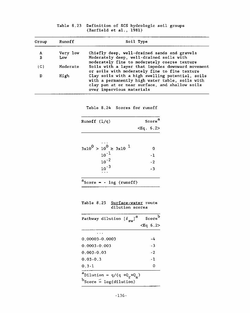
Table 8.23 Definition of SCS hydrologic soil groups (Barfield et al., 1981)
Group Run0 f f Soil Type
A Very low Chiefly deep, well-drained sands and gravels B Low Moderately deep, well-drained soils with
moderately fine to moderately coarse texture (C) Moderate Soils with a layer that impedes downward movement
or soils with moderately fine to fine texture D High Clay soils with a high swelling potential, soils
with a permanently high water table, soils with clay pan at or near surface, and shallow soils over impervious materials
Table 8.24 Scores for runoff
Runoff (l/q) Scorea <Eq. 6.2>
. . . 0 0 0 1 3x10 > 10 13x10
10-1
. . .
-1 -2 -3
a Score = - log (runoff)
Table 8.25 Surface-water route dilution scores
b
<Eq 6.2> Pathway dilution [ S l a Score sw
. . . 0.00003-0.0003 0.0003-0.003
0.003-0.03 0.03-0.3 0.3-1
-4
- 3
- 2
-1 0
a Dilution = q / ( q +Q +Q )
bScore log(di1ution) r a
-136-

I-
-
-
Table 8 . 2 6 Runoff curve numbers for selected agricultural, suburban, and urban land use (antecedent moisture condition 11) (USBR, 1977 and Barfield et al, 1 9 8 1 )
Land use Potential Hydrologic soil group for runoff A B tC1 D
Cultivated (newly reclaimed land) Row crops
Small grain
Legumes or rotation meadow
Pasture
Woods or farm woodlots
Meadow (permanent)
Western range land Grass-weed-mixture w/brush
Sagebrush w/grass understory
Juniper or pinon w/grass
Aspen, oak, or maple w/other mountain brush mixtures
Forest land
High Low High Low High Low High Low
High Low
High Low High Low High Low High LOW
High Medium Low
Developed land Open spaces (parks, golf, etc.) Medium
Business area ( 8 5 % impervious) Industrial area ( 7 5 % impervious) Residential: <1 /8 acre, 65% impervious
1 / 4 acre, 38% impervious 1/2 acre, 25% impervious 1 acre, 20% impervious
Low
Streets, roads, and parking lots Paved with curbs -normal climate
Gravel Dirt
-very warm climate
7 2 8 1 65 7 5 65 7 6 6 1 7 3 66 77 55 6 9 68 7 9 39 6 1
45 66 25 55
30 58
7 8 59 6 4 35 7 3 4 0 63 30
56 7 5 36 6 0 1 5 44
4 9 6 9 39 6 1 89 92 81 88 77 85 61 7 5 5 4 7 0 5 1 68
98 98 95 95 7 6 85 7 2 82
88 82 8 4 8 1 85 78 86 7 4
77 7 0
7 1
85 7 1 78 46 8 4 59 7 1 40
86 7 0 5 4
7 9 7 4 9 4 9 1 90 83 80 7 9
98 95 89 87
9 1 86 88 8 4 89 83 89 80
83 77
78
92 8 4
9 1 7 6 6 1
8 4 80 95 93 92 87 85 8 4
98 95 9 1 89
- 137 -
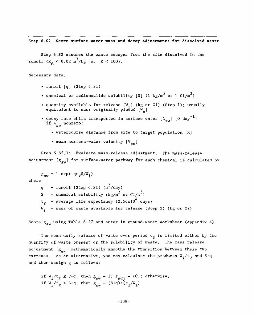
Step 6.S2 Score surface-water mass and decay adjustments for dissolved waste
Step 6.S2 assumes the waste escapes from the site dissolved in the 3 runoff (Kd < 0.02 m /kg or R < 100).
Necessary data.
runoff [q] (Step 6.S1)
chemical or radionuclide solubility [SI (1 kg/m3 or 1 Ci/m ) 3
quantity available for release [Wi] (kg or Ci) (Step 1); usually equivalent to mass originally placed [W ]
0 -1 decay rate while transported in surface water [ A ] ( 0 day ) sw if Asw nonzero:
watercourse distance from site to target population [XI mean surface-water velocity [V ] sw
SteD 6.S2.1: Evaluate mass-release adiustment. The mass-release adjustment [g ] for surface-water pathway for each chemical is calculated by sw
gsw = l-exp(-qtRS/W.) 1
q = runoff (Step 6.S1) (m /day) S = chemical solubility (kg/m3 or Ci/m )
tQ = average life expectancy (2.56~10 days)
Wi
where 3
3 4
= mass of waste available for release (Step 2) (kg or Ci)
Score g using Table 8.27 and enter in ground-water worksheet (Appendix A ) . sw
The mean daily release of waste over period t is limited either by the R quantity of waste present or the solubility of waste. adjustment [g,,] mathematically smooths the transition between these two extremes. As an alternative, you may calculate the products W./t and S * q
and then assign g as follows:
The mass release
i Q
if W./tR 1 I S - q , then gsw = 1; Fadj = ( 0 ) ; otherwise, if Wi/tQ > S*q, then gsw = (S*q)*(tR/Wi)
-138-

SteD 6.S2.2 : Find fraction of waste dissolved. Estimate the fraction of waste dissolved and removed [ p ] as follows and score with Table 8 .28 . dis
r - net 'dis 7 a
-
Step 6.S2.3: Evaluate decav. Although usually insignificant, score decay while transported in surface water as follows (where a - surface- water dispersivity = 0.6 d 5/6 r iv
sw (1 m)) <Derivation of Scoring Model,
Chapter 6>. If aswXsw/Vsw < 0 . 2 5 , then
Score IFdecay 3 - nearest integer of [ - Xriv 6 ' s ; ] sw sw 2 . 3
otherwise,
Score [Fdecay1 = nearest integer of [ - Xriv 'sw ] 2 . 3 vsw
Table 8 .27 Mass-release adjustment scores for surface-water route
b Release adjustment [ g] a Score . . .
0 .003-0 .03
0 .03 -0 .3
0 . 3 - 1
- 2
-1
(01
a
bScore = log(adjustment) Adjustment = 1-exp(-q taS/wi)
- 139 -
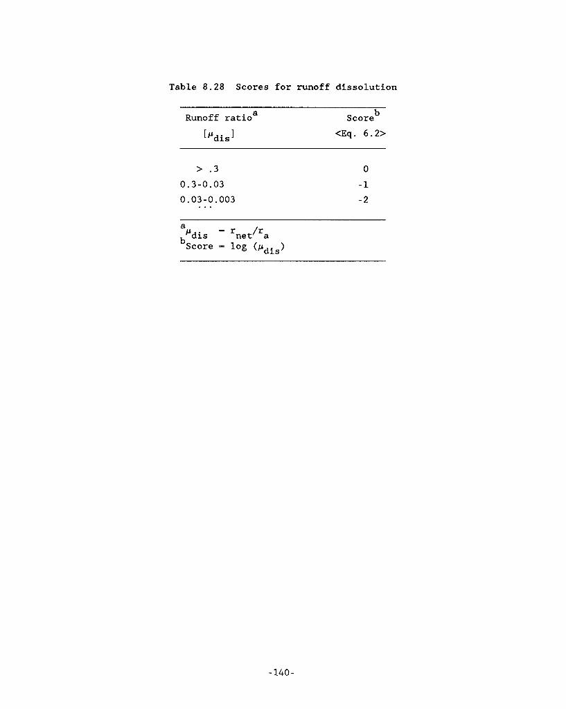
Table 8.28 Scores for runoff dissolution
Runoff ratioa
[’dis
b Score <Eq. 6.2>
> . 3
0.3-0.03 0.03-0 .003 . . .
0
-1 - 2
a
bScore - l og (pdis) ’dis rnet’ra
-140-

Step 6.S3. Score surface-water sediment yield and decay for adsorbed waste
Rather than assume that the waste is dissolved in the runoff, this step
Kd ' assumes that the waste is adsorbed onto sediment particles (R > 100; 0.02 m /kg). 3
Necessarv data
2 sediment yield [Y,] (0.5 kg/m /yr) or if unavailable,
SCS rainfall erosivity factor [RE] (150) (available from local U.S. Soil Conservation Service (SCS) office or Figure 8.7)
SCS control-practice factor [CP] (0.35) (local SCS office or Table 8.29)
SCS length-slope topographic factor [LS] (0.4) (local SCS office or Figure 8.8)
c
c
Step 6.S3.1: Estimate sediment yield if necessary. If sediment yield 2 data are lacking, estimate the annual sediment yield [Y,] (kg/m /yr) as
follows <Derivation of Scoring Model, Chapter 6>
Ys =;: 5 . 6 ~ 1 0 - ~ CP LS RE
Check value with Table 8 . 2 9 . Reduce the sediment yield [Y,] to a maximum of 100 times average basin yield (Table 8.30) if it exceeds this value. Increase the sediment yield [Y ] to a minimum low basin yield (Table 8.30) if it is smaller. Score Ys with Table 8.31.
S
100 basinav 5 Ys 5 basin low
SteD 6.S3.2: Find fraction of waste carried away with sediment. The fraction of waste removed is the ratio of annual sediment yield [Y ] to original mass of erodible soil per unit area [ p h], where pb is bulk density of the soil (1500 kg/m 1 and h is soil depth subject to erosion annually (0.01 m):
S
b 3
Y Y * s = s "soil - pbh l5
-141-
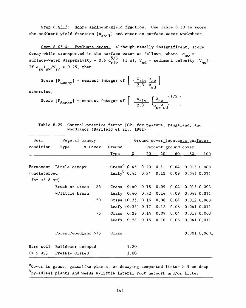
Step 6.S3.3: Score sediment-yield fraction. Use Table 8.30 to score the sediment yield fraction [psoil] and enter on surface-water worksheet.
SteD 6.S3.4: Evaluate decav. Although usually insignificant, score decay while transported in the surface water as follows, where a =
surface-water dispersivity = 0 . 6 d 5'6
If aswXsw/Vsd
sw (1 m), Vsd = sediment velocity (V ) . r iv sw
C 0 . 2 5 , then
"Ore [ Fdecay 1 - nearest integer of [ - Xriv 'sw ] 2.3 Vsd
otherwise, 1 / 2
Score [ F ~ ~ ~ ~ ~ J = nearest integer of [ - Xriv [aXs; ] ] sw sd 2 . 3
Table 8.29 Control-practice factor [CP] for pasture, rangeland, and woodlands (Barfield et al., 1981)
~- ~~
Soil Vegetal canopv Ground cover (contacts surface) condition Type % Cover Ground Percent ground cover
TvDe 0 20 40 60 80 100
a Permenant Little canopy Grass 0 . 4 5 0 . 2 0 0.11 (undisturbed Leafyb 0 . 4 5 0.24 0 . 1 5
for > 5 - 8 yr) Brush or trees 2 5 Grass 0.40 0.18 0.09 w/li t tle brush Leafy 0 . 4 0 0 . 2 2 0 . 1 4
50 Grass ( 0 . 3 5 ) 0.16 0.08 Leafy (0.35) 0.17 0 . 1 2
75 Grass 0.28 0 . 1 4 0 . 0 9
Leafy 0 . 2 8 0 . 1 5 0.10
0 . 0 4
0 . 0 9
0 . 0 4
0 . 0 9
0 . 0 4
0.08 0 . 0 4
0.08
0 . 0 1 3 0 .003
0.043 0 . 0 1 1
0.013 0.003 0 . 0 4 3 0.011 0.012 0 . 0 0 3
0 . 0 4 1 0.011
0.012 0 . 0 0 3
0 . 0 4 1 0.011
Forest/woodland >75 Grass 0.001 0.0001
Bare soil Bulldozer scraped 1.20
(> 5 yr) Freshly disked 1.00
a
bBroadleaf plants and weeds w/little lateral root network and/or litter Cover is grass, grasslike plants, or decaying compacted litter > 5 cm deep
-142-
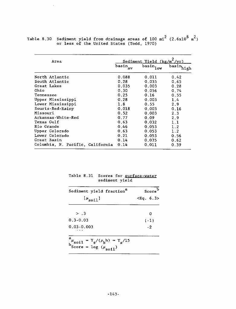
8 2 Table 8 . 3 0 Sediment yield from drainage areas of 100 mi2 ( 2 . 6 ~ 1 0 or less of the United States (Todd, 1 9 7 0 )
m )
Area Sediment Yield (kdm2/yr bas in bas in av low
North Atlantic 0 . 0 8 8 South Atlantic 0 . 2 8 Great Lakes 0 . 0 3 5 Ohio 0 . 3 0 Tenne s s e e 0 . 2 5 Upper Mississippi 0 . 2 8 Lower Mississippi 1 . 8 Souris-Red-Rainy 0 . 0 1 8 Missouri 0 . 5 2 Arkansas-White-Red 0.77 Texas Gulf 0 . 6 3 Rio Grande 0 . 4 6 Upper Colorado 0 . 6 3 Lower Colorado 0 . 2 1 Great Basin 0 . 1 4 Columbia, N. Pacific, California 0.14
0.011 0 . 0 3 5 0 . 0 0 3 0 . 0 5 6 0 . 1 6 0 . 0 0 3 0 . 5 5 0 . 0 0 3 0 . 0 0 3 0 . 0 9 0 . 0 3 2 0 . 0 5 3 0 . 0 5 3 0 . 0 5 3 0 .035 0.011
0 . 4 2 0 . 6 5 0.28 0 . 7 4 0 . 5 5 1 . 4 2 . 9 0 .16 2 . 3 2 . 9 1.1 1.2 1 . 2 0 . 5 6 0 . 6 2 0 . 3 9
Table 8 . 3 1 Scores for surface-water sediment yield
b
[psoill <Eq. 6 .3>
Sediment yield fractiona Score
> . 3
0 . 3 - 0 . 0 3
0 . 0 3 - 0 . 0 0 3 . . .
0
(-1) -2
a
bScore = l o g ( p
psoil = Ys/(Pbh) ys/15
soil
- 1 4 3 -
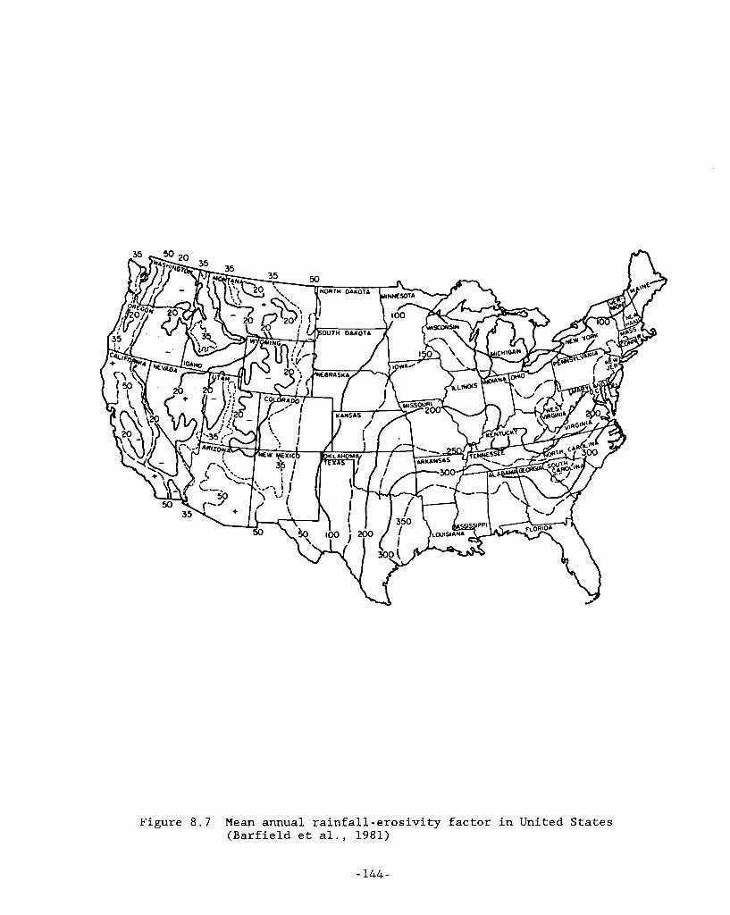
Figure 8.7 Mean annual rainfall-erosivity factor in United States (Barfield et al., 1981)
- 144 -
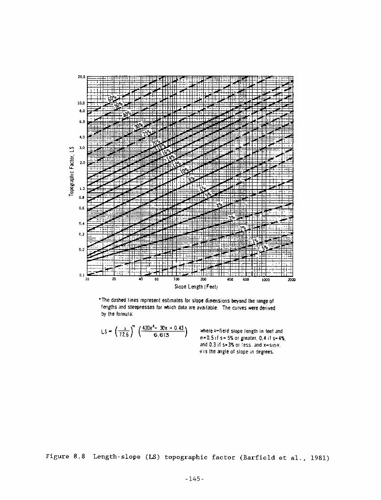
20s
10.0
8.0
6.0
WY -1
4.0
3.0
c
2.0
1.0
0.8
0.6
0.4
0.3
0.2
0.1
Slope Length (Feet)
'The dashed lines represent estimates for slope dimensions beyond the range of lengths and steepnesses for which data a:e avallable. The curves were derived by the formula:
430x2+ 30x + 0.43) whereA-field slope length in feet and m-0.5 i f s- 5% or greater. 0 . 4 i f s-4%, and 0.3 i f s-3% or less, and x-sin@. e i s the angle of slope in degrees.
Ls- (&r ( 6.613
Figure 8.8 Length-slope (LS) topographic factor (Barfield et al., 1981)
- 145 -
Step 6.A1. Assume mass-release adjustment
Only the waste-specific, mass-release adjustment factor [gal must be evaluated in Step 6 for the air pathway. Because the air pathway is seldom of major importance, first assume the score [Fadj] for the mass-release adjustment [g ] is zero and skip Step 6.A2. The air pathway score is readily completed. Should the air pathway determine the site score (highest pathway score), return to Step 6, estimate [gal as described in Step 6.A2, and adjust the air pathway.
a
- 146 -
Step 6.A2. Calculate mass-release adjustment
Necessarv data
quantity of waste available for release [Wi] (kg or Ci)
vaporization emission rate [ev], or if unavailable:
vapor pressure of volatile chemical [p]
mass concentration 1. = 'i 1 L
pdc ntAsJ area of surface containing Razardous vapor [A ] S
gram molecular weight of chemical [w,]
cover reduction factor [f ] estimated in Step 6.A2.1 covr gas generation factor [f ] estimated in Step 6.A2.5
gen fugitive dust emission rate [ew], or if unavailable
Thornthwaite precipitation-effectiveness index (PE) (Figure 8.9) (60)
fraction of covered soil [ p ] (bare, = 0) (unbroken grass prevents particle resuspension, covr p - ,I;covr
covr
The mass-release adjustment factor [g ] depends upon the emission rate a of waste into the atmosphere. The emission rate [e] of chemical waste to the air pathway is the sum of the volatilization rate [e 1 , wind erosion rate [ew], and any contribution from dust generated by vehicular traffic. all the pathways, the rate of waste release is important information but measured data are often scarce and/or precise calculation techniques are time-consuming and data intensive. For the air pathway, estimate the emission rates from
V As with
measured data;
empirical equations provided;
.-
other empirical equations for which data are available [for example, USDA wind erosion equation (Skidmore and Woodruff, 1968)], particulate emission rate equations (Cowherd et al., 1985), vapor emission rate equations (Mackay, 1980; Shen, 1981; EPA, 1982).
- 147 -
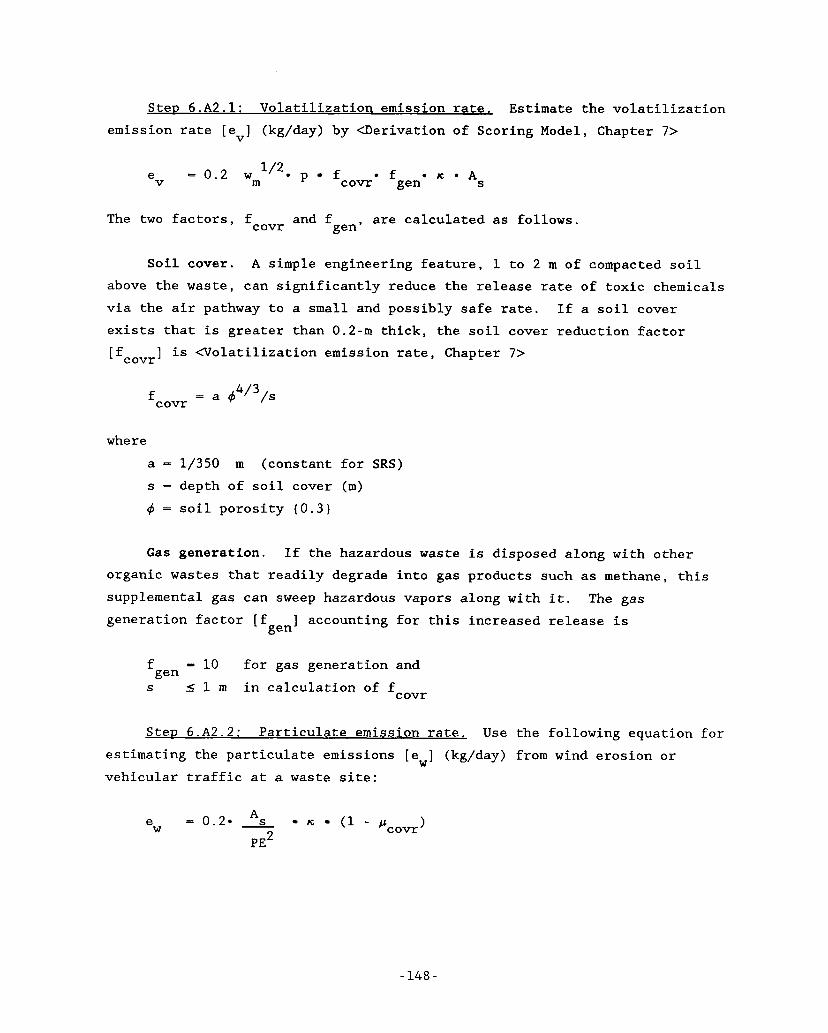
SteD 6.A2.1: Volatilization emission rate. Estimate the volatilization emission rate [e J (kg/day) by <Derivation of Scoring Model, Chapter 7>
V
e - 0.2 wm 1/2. o f * K . A ~ P fcovr gen V
and fgen. are calculated as follows. covr The two factors,
S o i l cover. above the waste, can significantly reduce the release rate of toxic chemicals via the air pathway to a small and possibly safe rate. exists that is greater than 0.2-m thick, the soil cover reduction factor
[ covr
A simple engineering feature, 1 to 2 m of compacted soil
If a soil cover
J is <Volatilization emission rate, Chapter 7>
= a fcovr
where a = 1/350 s - depth
d 4 i 3 / S
m (constant for SRS) of soil cover (m)
q5 = soil porosity (0.3)
Gas generation. If the hazardous waste is disposed along with other organic wastes that readily degrade into gas products such as methane, this supplemental gas can sweep hazardous vapors along with it. generation factor [f J accounting for this increased release is
The gas
gen
f = 10 for gas generation and S 5 1 m in calculation of fcovr gen
S t e p 6.A2.2: Particulate emission rate. Use the following equation for estimating the particulate emissions [ e ] (kg/day) from wind erosion or vehicular traffic at a waste site:
W
e = 0.2. As K (’ - pcovr ) w PE2
- 148 -
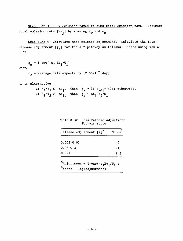
SteD 6.A2.3: Sum emission rates to find total emission rate. Estimate total emission rate [Ce.] by summing ev and e . J W
SteD 6.A2.4 Calculate mass-release adiustment. - Calculate the mass- release adjustment [g ] for the air pathway as follows. Score using Table 8.32:
a
ga = l-exp(-tR Ce./wi)
tR = average life expectancy (2.56~10~ day]
J where
As an alternative, then ga = 1; Fadj= (0); otherwise, j’
j, J
If W./tR I Ce 1
If Wi/tR > Ce then ga - Ce. t p i
Table 8.32 Mass-release adjustment for air route
~~ ~
b Release adjustment [ g] a Score . . .
0.003-0.03 0.03-0.3 0.3-1
-2 -1 (0)
a b Adjustment = 1-exp(-t Ee./w. )
Score = log(adjustment) R J 1
- 149 -
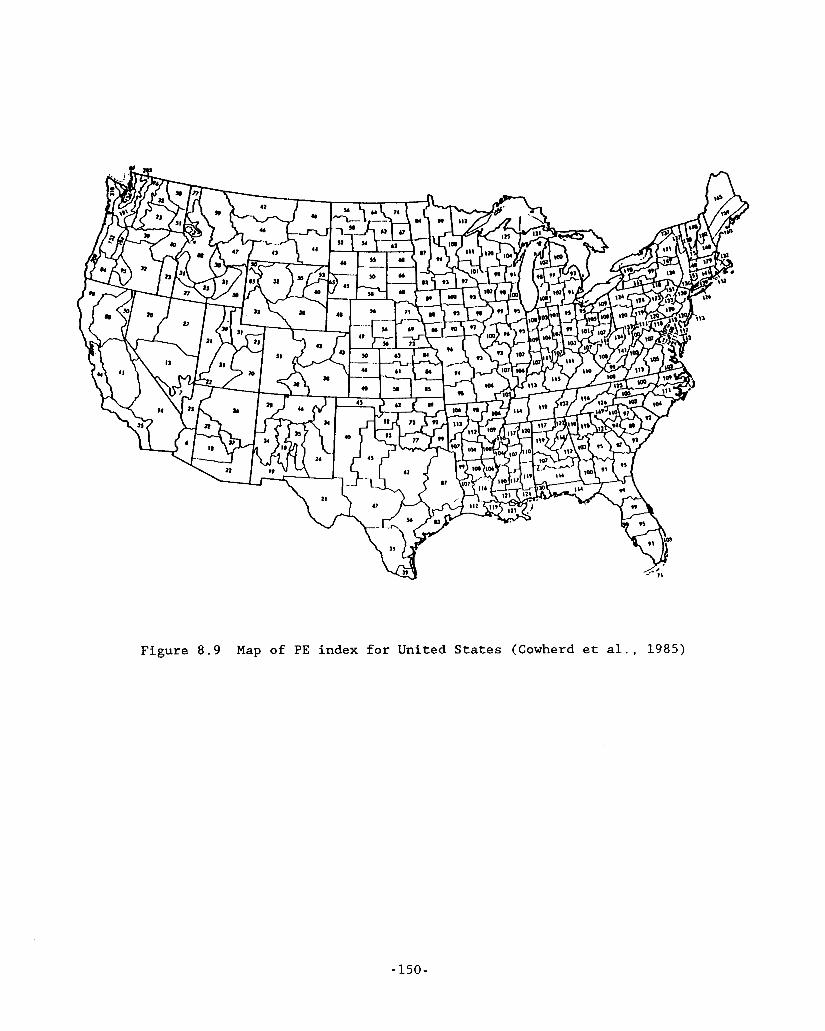
Figure 8.9 Map of PE index for United States (Cowherd et al., 1985)
-150-

.^ ~
_I”.-
-
Step 7 . Combine chemical scores then pathway scores to obtain site score
Part a: Combine individual chemical scores to obtain Dathwav score. To evaluate a scenario score (for example, one of several in the ground-water pathway group), start with the highest individual chemical score for that scenario. Then account for the number of chemicals with this score or one lower as follows:
F + 0.1 na + 0.01 II,, + a . . .
where F - scenario score Fa n a II,,
seq - highest individual score (for example, chemical a) = number of other chemicals with same score Fa = number of chemicals with next highest score F - Fa- 1 b
Next evaluate the pathway score as
= F + 0.1 n + 0.01 n2 + . . . Fpath 1 1
18.31
~3.41
where - pathway score (for example, ground-water pathway) = highest individual score (for example, scenario 1)
Fpath Fa n = number of other scenarios with same score F a %
1 - Fa- 1 b = number of scenarios with next highest score F
Equation [8.4] has omitted the score for the contants [F ] because they were roughly equivalent, that is,
r
- 3 for ground-water pathway <constants of model eq. [5.1]> - 3 for surface-water pathway <eq. [6.2]> = t - 3 for air pathway <eq. [7.2]>
Fr
Part b: Evaluate site score. The site score is the highest score among the three pathways unless two or more are identical, in which case raise the score by one unit.
-151-
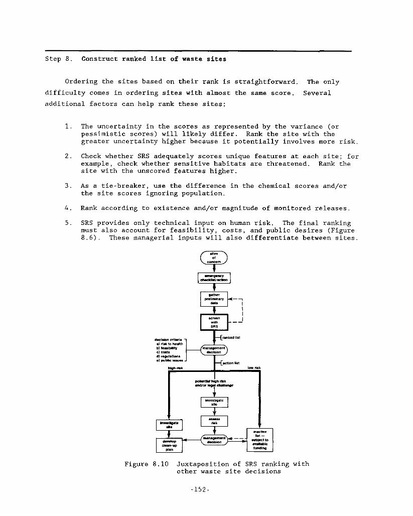
Step 8. Construct ranked list of waste sites
Ordering the sites based on their rank is straightforward. The only difficulty comes in ordering sites with almost the same score. Several additional factors can help rank these sites:
1. The uncertainty in the scores as represented by the variance (or pessimistic scores) will likely differ. Rank the site with the greater uncertainty higher because it potentially involves more risk.
2. Check whether SRS adequately scores unique features at each site; for example, check whether sensitive habitats are threatened. Rank the site with the unscored features higher.
3 . As a tie-breaker, use the difference in the chemical scores and/or the site scores ignoring population.
4 . Rank according to existence and/or magnitude of monitored releases.
5. SRS provides only technical input on human risk. The final ranking must also account for feasibility, costs, and public desires (Figure 8 . 6 ) . These managerial inputs will also differentiate between sites.
Figure 8.10 Juxtaposition of SRS ranking with other waste site decisions
-152 -
9. COMPARISON OF SRS WITH OTHER ASSESSMENT SCHEMES
Following are three hypothetical examples where we apply SRS. Although the examples illustrate the use of SRS, when learning SRS, refer to Appendix B, which shows completed worksheets for an actual Superfund site. compare SRS results with results from other ranking and rapid assessment techniques. However, because the SRS scores must be converted to concentrations, the calculations are not straightforward unless familiar with the equations in Chapters 5 , 6, and 7.
Here we
The comparisons serve to verify SRS to a limited extent.
--
I
-..-
I
c
Three HvDothetical Sites Contaminating Ground Water
Whelan et al. (1985, 1986) present three simplified cases of contaminant migration through the ground water to demonstrate differences between HRS, mHRS, and the more detailed RAPS ranking system. Applying SRS to these same three sites, we demonstrate its ability to rank sites similar to RAPS.
Site description. The following text briefly summarizes detailed discussion found in Whelan et al. (1985, 1986) for each of the three sites. In general, the simplified sites formulated by Whelan et al. (1985, 1986) primarily looked at differences in migration once the contaminant left the site; numerous other features were identical between sites. For example, all sites involved two wastes, arsenic and strontium-90, each at quantities such that the chemical health risk of each waste, W o e Toral, was the same. Furthermore, the exposed population, climatic conditions, and aquifer properties were identical.
At sites 1 and 2, the mixture of chemical and radioactive sludge containing arsenic and strontium-90 is stored in unlined landfills. The bottom of the landfills coincide with the top of an unconsolidated, unconfined sand aquifer. At site 1, 500 people obtains all its water from wells located 1 km directly downgradient of the waste site [N = 500 , x - 1000 m]; at site 2 , 500 people obtain water from wells 6 km downgradient from the site, rather than 1 km [N - 500, x - 6000 m].
gw
gw
At site 3 , the same mixture of arsenic and strontium-90 is stored in an unlined landfill, but the landfill lies 6 m above, rather than directly in
-153 -
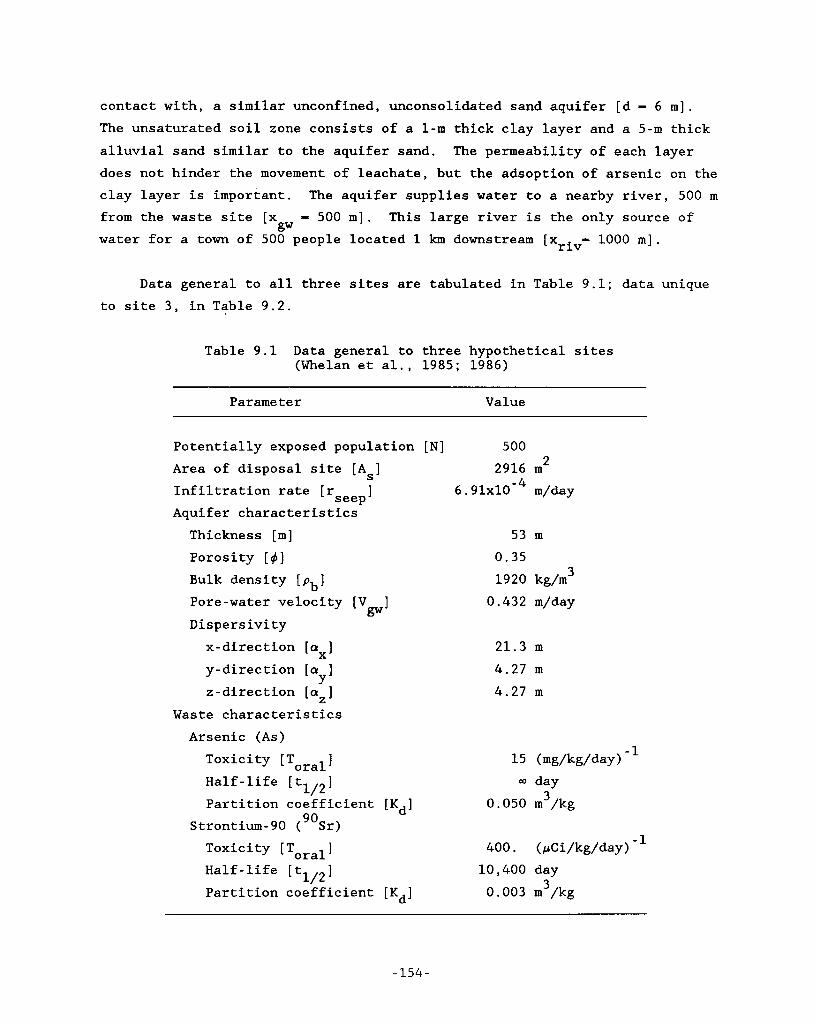
contact with, a similar unconfined, unconsolidated sand aquifer [d = 6 m]. The unsaturated soil zone consists of a 1-m thick clay layer and a 5-m thick alluvial sand similar to the aquifer sand. The permeability of each layer does not hinder the movement of leachate, but the adsoption of arsenic on the clay layer is important. The aquifer supplies water to a nearby river, 500 m from the waste site [x = 500 m]. This large river is the only source of water for a town of 500 people located 1 km downstream [xriv= 1000 m].
gw
Data general to all three sites are tabulated in Table 9.1; data unique to site 3, in Table 9.2.
Table 9.1 Data general to three hypothetical sites (Whelan et al., 1985; 1986)
Parameter Value
Potentially exposed population [N] 500 Area of disposal site [As] Infiltration rate [r ] 6.91~10-~ m/day Aquifer characteristics
2916 m2
seep
Thickness [m] 53 m Porosity [d] 0.35 Bulk density [ p ] 1920 kg/m3 Pore-water velocity [V ] 0.432 m/day Dispersivity
b
gw
x-direction [a ] 21.3 m y-direction [a ] 4.27 m z-direction [a ] 4.27 m
X
Y Z
Waste characteristics Arsenic (As)
Toxicity [T ] 15 (mg/kg/day) oral Half-life [tlI2] Q) day Partition coefficient [Kd] 3 0.050 m /kg
Strontium-90 (90~r) Toxicity [T ] oral 400. (pCi/kg/day) Half-life [tl/2] 10,400 day Partition coefficient [Kd] 3 0.003 m /kg
-154-
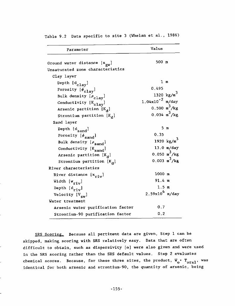
Table 9.2 Data specific to site 3 (Whelan et al., 1986)
Par ame t e r Value
Ground water distance [x ] 500 m gw
Unsaturated zone characteristics Clay layer
l m 0.495
2
Depth [dclayl Porosity [ d clay 3 Bulk density [ pclay] 1320 kg/m” Conductivity [K ] 1.04~10- m/day
Arsenic partition [Kd] 0.500 m /kg
Strontium partition [Kd] 0.034 m /kg
clay 3
3
Sand layer
Depth 1 ds and 1 Porosity Bulk density [psand] Conductivity [K s and ] Arsenic partition [Kd] Strontium partition [K d 1
River characteristics River distance [xriv] Width [wriv]
Velocity [V sw ] Depth [drivl
5 m 0.35 1920 kg/m 3
13.0 m/day 0.050 m /kg 0.003 m3/kg
3
1000 m 91.4 m 1.5 m
2.59~10 4 m/day
Water treatment Arsenic water purification factor 0.7
Strontium-90 purification factor 0.2
SRS Scoring. - Because all pertinent data are given, Step 1 can be Data that are often skipped, making scoring with SRS relatively easy.
difficult to obtain, such as dispersivity [a] were also given and were used in the SRS scoring rather than the SRS default values. chemical scores. identical for both arsenic and strontium-90, the quantity of arsenic, being
Step 2 evaluates Because, for these three sites, the product, Woe Toral, was
-155-
.____ .
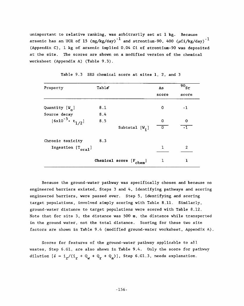
unimportant to relative ranking, was arbitrarily set at 1 kg. arsenic has an UCR of 15 (mg/kg/day)-' and strontium-90, 400 (pCi/kg/day)-' (Appendix C), 1 kg of arsenic implied 0.04 Ci of strontium-90 was deposited at the site. The scores are shown on a modified version of the chemical worksheet (Appendix A) (Table 9.3).
Because
Table 9.3 SRS chemical score at sites 1, 2, and 3
Property Tab16 As score score
Quantity [W ] 8.1 Source decay 8.4
0 0 -1
[ 6 ~ 1 0 - ~ * tl,2] 8.5 0 0 Subtotal [Wi] 0 -1
Chronic toxicity 8.3 Ingestion [T ] oral
Chemical score [ F ] chem
1 2
1 1
Because the ground-water pathway was specifically chosen and because no engineered barriers existed, Steps 3 and 4 , identifying pathways and scoring engineered barriers, were passed over. Step 5 , identifying and scoring target populations, involved simply scoring with Table 8.11. Similarly, ground-water distance to target populations were scored with Table 8.12. Note that for site 3, the distance was 500 m, the distance while transported in the ground water, not the total distance. Scoring for these two site factors are shown in Table 9.4 (modified ground-water worksheet, Appendix A ) .
Scores for features of the ground-water pathway applicable to all wastes, Step 6.G1, are also shown in Table 9.4. Only the score for pathway dilution [6 = ir/(ir + Qw + Qr + Qa)], Step 6.G1.3, needs explanation.
-156-
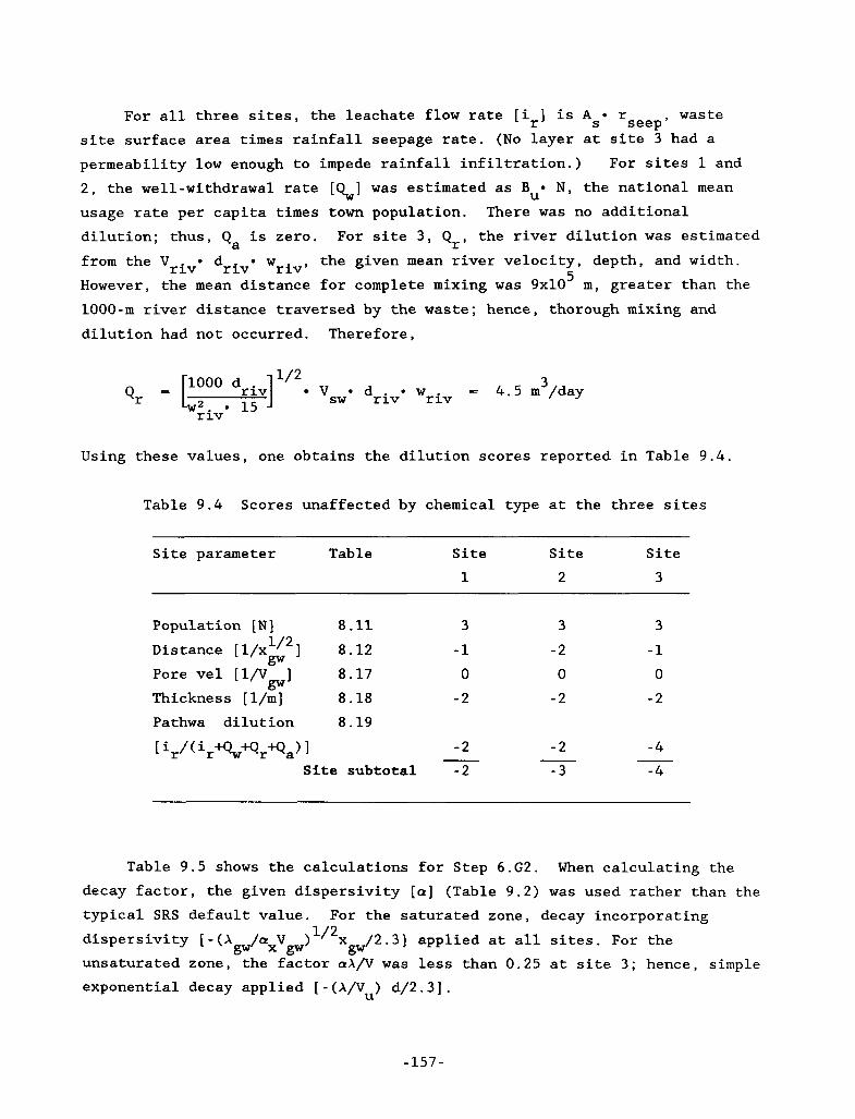
I
I-
F'
For all three sites, the leachate flow rate [i,] is As* rseep, waste
site surface area times rainfall seepage rate. (No layer at site 3 had a permeability low enough to impede rainfall infiltration.) 2 , the well-withdrawal rate [QJ was estimated as B N, the national mean usage rate per capita times town population. dilution; thus, Qa is zero. from the Vriv* driV* wriv, the given mean river velocity, depth, and width. However, the mean distance for complete mixing was 9x10⁵ m, greater than the 1000-m river distance traversed by the waste; hence, thorough mixing and dilution had not occurred. Therefore,
For sites 1 and
U There was no additional
For site 3 , Q,, the river dilution was estimated
3 - 4.5 m /day r iv Vsw* drive w = ['OOO driv] 1/2
Qr wziV* 15
Using these values, one obtains the dilution scores reported in Table 9.4.
Table 9.4 Scores unaffected by chemical type at the three sites
Site parameter Table Site Site Site 1 2 3
Population [N] 8.11 3 3 3 Distance [l/x 8.12 -1 - 2 -1
gw Pore vel 1 8.17 0 0 0 Thickness [l/m] 8.18 -2 - 2 - 2
gw
Pathwa dilution 8.19 -2 - 2 -4
Site subtotal -2 - 3 -4 - - ir/(ir+gu+Q,+Qa) 1
Table 9.5 shows the calculations for Step 6.G2. When calculating the decay factor, the given dispersivity [a] (Table 9.2) was used rather than the typical SRS default value. For the saturated zone, decay incorporating dispersivity [ - ( A /a V )1/2x&2.3] applied at all sites. For the
gw x gw unsaturated zone, the factor a A / v was less than 0.25 at site 3; hence, simple exponential decay applied [-(Anu) d/2.3].
-157 -
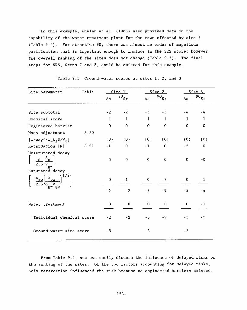
I n t h i s example, Whelan e t a l . (1986) a l s o provided d a t a on t h e
c a p a b i l i t y of t h e water t r ea tmen t p l a n t f o r t h e town e f f e c t e d by s i t e 3
(Table 9 . 2 ) . For s t ron t ium-90 , t h e r e w a s a lmost an o r d e r of magnitude
p u r i f i c a t i o n t h a t i s impor tan t enough t o inc lude i n t h e SRS s c o r e ; however,
t h e o v e r a l l ranking o f t h e s i tes does n o t change (Table 9 . 5 ) . The f i n a l
s t e p s f o r SRS, S teps 7 and 8 , could be omi t ted f o r t h i s example.
Table 9 . 5 Ground-water s c o r e s a t s i tes 1, 2 , and 3
S i t e parameter Table S i t e 1 S i t e 2 S i t e 3
AS 90sr A s 9 0 ~ r A s 9 0 ~ r
S i t e s u b t o t a l - 2 - 2
Chemical s c o r e 1 1
Engineered b a r r i e r 0 0
Mass adjus tment 8 .20
[ 1 - e x p ( - i t S/Wi] ( 0 ) ( 0 ) r l R e t a r d a t i o n [ R ] 8 . 2 1 -1 0
Unsa tura ted decay x
[ 2 . 3 V
S a t u r a t e d decay
0 0 - d 2-1 gw
Water t r ea tmen t
0 -1
- 2 - 2
- -
0 0
I n d i v i d u a l chemical s c o r e - 2 - 2
Ground-water s i t e s c o r e - 5
- 3 - 3
1 1
0 0
0 0
0 - 7 - -
- 3 -9
0 0 - -
- 3 -9
- 6
-4 - 4
1 1
0 0
0 -0
0 -1 _ _ ~
- 5 - 4
0 -1 - -
- 5 - 5
-8
From Table 9 . 5 , one can e a s i l y d i s c e r n t h e i n f l u e n c e of de layed r i s k s on
t h e ranking of t h e s i t e s . O f t h e two f a c t o r s account ing f o r de layed r i s k s ,
on ly r e t a r d a t i o n in f luenced t h e r i s k because no engineered b a r r i e r s e x i s t e d .
- 158 -
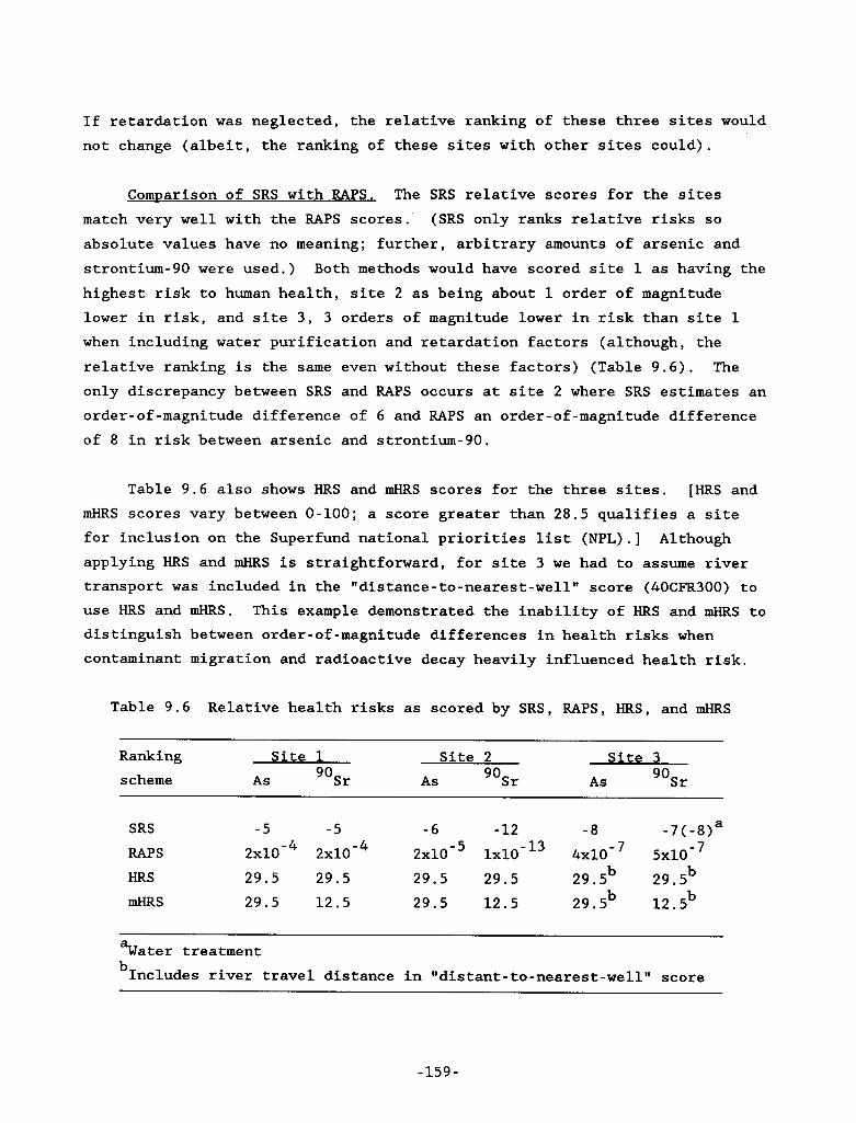
- -
I
Y
c
I
--
I
If retardation was neglected, the relative ranking of these three sites would not change (albeit, the ranking of these sites with other sites could).
Comparison of SRS with RAPS. The SRS relative scores for the sites match very well with the RAPS scores. (SRS only ranks relative risks so absolute values have no meaning; further, arbitrary amounts of arsenic and strontium-90 were used.) Both methods would have scored site 1 as having the highest risk to human health, site 2 as being about 1 order of magnitude lower in risk, and site 3, 3 orders of magnitude lower in risk than site 1 when including water purification and retardation factors (although, the relative ranking is the same even without these factors) (Table 9.6). The only discrepancy between SRS and RAPS occurs at site 2 where SRS estimates an order-of-magnitude difference of 6 and RAPS an order-of-magnitude difference of 8 in risk between arsenic and strontium-90.
Table 9.6 also shows HRS and mHRS scores for the three sites. [HRS and mHRS scores vary between 0-100; a score greater than 28.5 qualifies a site for inclusion on the Superfund national priorities list (NPL).] Although applying HRS and mHRS is straightforward, for site 3 we had to assume river transport was included in the "distance-to-nearest-well" score (40CFR300) to use HRS and mHRS. This example demonstrated the inability of HRS and mHRS to
distinguish between order-of-magnitude differences in health risks when contaminant migration and radioactive decay heavily influenced health risk.
Table 9.6 Relative health risks as scored by SRS, RAPS, HRS, and mHRS
Ranking Site 1 Site 2 Site 3 scheme As As As
SRS -5 -5 -6 - 12 - 8 -7( -8)a
HRS 29.5 29.5 29.5 29.5 29.5b 29.5b mHRS 29.5 12.5 29.5 12.5 29.5b 12.5b
RAPS 2x1~-4 2x1~-4 2x1~-5 1 ~ 1 0 - l ~ 4x1~-7 5x1~-7
%a ter treatment bIncludes river travel distance in "distant-to-nearest-well" score
-159-
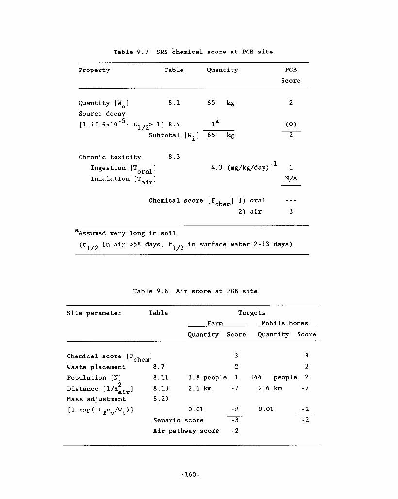
Table 9 . 7 SRS chemical score at PCB site
Property Table Quantity PCB Score
Quantity [ Wo ] 8 . 1 65 kg Source decay [l if 6 ~ 1 0 - ~ * tlI2> 11 8 . 4 la
Subtotal [Wi] 65 kg
2
Chronic toxicity Ingestion [Torall Inhalation [Tair]
8 . 3
Chemical score
4 . 3 (mg/kg/day)-' 1
N/A
_ _ _ [Fcheml Oral 2) air 3
a Assumed very long in soil (tl,2 in air >58 days, tlI2 in surface water 2-13 days)
Table 9 . 8 Air score at PCB site
Site parameter Table Targets Farm Mobile homes
Quantity Score Quantity Score
Chemical score [F ] 3 Waste placement 8 . 7 2
chem
Population [ N] 8 . 1 1 3 . 8 people 1 144 people 2 Distance [l/xair]
Mass adjustment 8 . 2 9
8 . 1 3 2.1 km -7 2 . 6 km
[ 1 - exp ( - tfV/Wi> 1 0.01 - 2 0.01 -
Senario score - 3 - 2
Air pathway score - 2
3
2 2 -7
-2
-160-
HvDothetical Site Affecting: - Air Oualitv
c
Cowherd et al. (1985) present an example to illustrate their emergency response methodology which we repeat. Here, their unnamed contaminant is assumed to be polychlorinated biphenols (PCBs).
A hypothetical site, storing abandoned transformers leaking PCB, near North Platte, Nebraska, is among several sites the state wishes to clean up. A site survey reveals about 6.4 pprn contamination to 0.15 m below the surface spread over an area of 150 by 300 m. The soil is essentially unvegetated, and consists of easily eroded finely divided material without surface crusting. No tire track or ruts were found in the area. The nearest residences are the Loner farm, 2.1 km NW of the site, and 38 mobile homes, 2.6 k m NE of the site. Winds usually come out of the south.
Inhalation of soil particles impregnated with PCB is the assumed exposure scenario for this example. Table 9.7 presents the SRS chemical scores (Step 2 ) . The 65 kg of PCB was estimated from the measured contamination (6.4 ppm) by assuming a default soil bulk density [pb] of 1500 kg/m (default) and a bulk soil volume of 6750 m (150*300*0.15). Because only ingestion toxicity data were available for PCB, they were used for inhalation toxicity of PCB, also.
3 3
Table 9.8 shows steps 4, 5, and 6 of the SRS scoring for this Nebraska site. Although Step 3, selecting important pathways and sequences, is the next step, it was irrelevant to this example. Step 4 for the air route considers the type of waste placement of the waste. unspecified surface disposal, the release of 1. ~ x I O - ~ kg/day calculated below (Step 6.A2.2) is equivalent to -0.32 mg/kg/day (PCB concentration in half sphere above contaminated surface times daily inhalation rate [B 1 , a hundred thousand times greater than the allowable daily intake (ADI) of 2 . 3 ~ 1 0 - ~ mg/kg/day [10-5/UCR], assuming a cancer risk of 10 . Consequently, the monitored soil concentration (6.4 ppm) suggests a significant health hazard at the site and results in a score of 2 (Table 8 . 7 , Chapter 8).
Although the site is an
a
-5
From the site description, only the number of residences was known and so the national average of 3.8 persons per residence was used to estimate the persons potentially affected (Step 5).
-161-
-. "._l ._ .
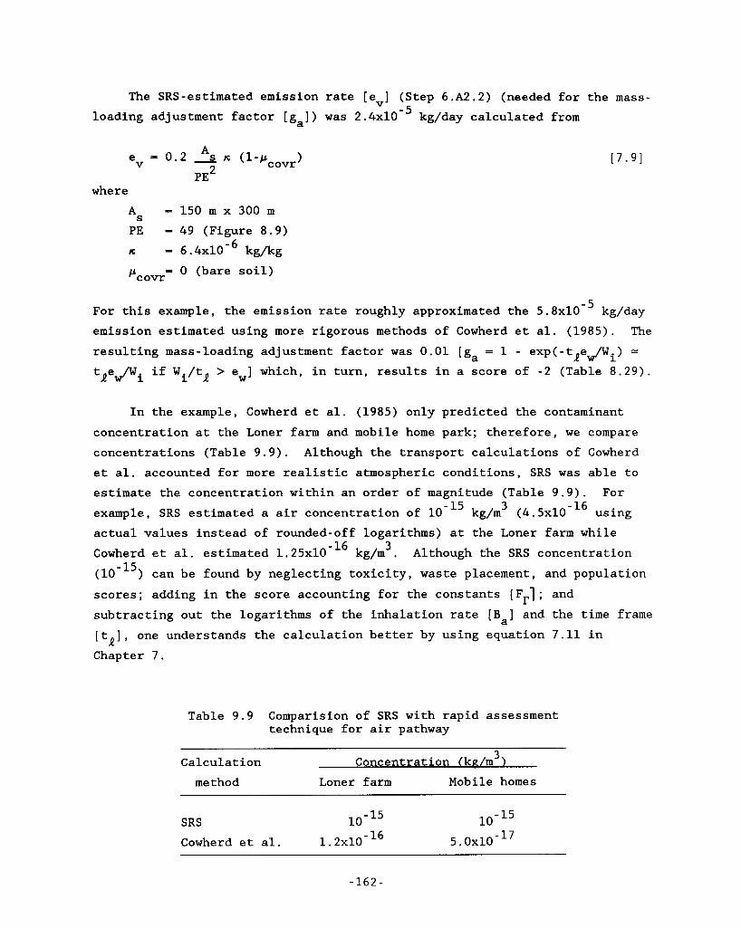
The SRS-estimated emission rate [e,] (Step 6.A2.2) (needed for the mass- loading adjustment factor [ gal ) was 2 . ~ x I O - ~ kg/day calculated from
A
PE2 e - 0.2 n ( 1 - p ) V covr
where
As PE - 49 (Figure 8.9) n - 6.4~10-~ kg/kg
pcovr
- 150 m x 300 m
- 0 (bare soil) -5 For this example, the emission rate roughly approximated the 5.8~10 kg/day
emission estimated using more rigorous methods of Cowherd et al. (1985). resulting mass-loading adjustment factor was 0.01 [ga = 1 - exp(-t,ew/Wi) =
t,ew/Wi if Wi/t, > ew] which, in turn, results in a score of -2 (Table 8.29).
The
In the example, Cowherd et al. (1985) only predicted the contaminant concentration at the Loner farm and mobile home park; therefore, we compare concentrations (Table 9.9). Although the transport calculations of Cowherd et al. accounted for more realistic atmospheric conditions, SRS was able to estimate the concentration within an order of magnitude (Table 9.9). For example, SRS estimated a air concentration of 10 actual values instead of rounded-off logarithms) at the Loner farm while
- 16 3 Cowherd et al. estimated 1.25~10 kg/m . Although the SRS concentration
- 15 3 kg/m (4.5~10-l~ using
can be found by neglecting toxicity, waste placement, and population scores; adding in the score accounting for the constants [Frl ; and subtracting out the logarithms of the inhalation rate [B,] and the time frame [t,], one understands the calculation better by using equation 7.11 in Chapter 7.
Table 9.9 Comparision of SRS with rapid assessment technique for air pathway
3 Calculation Concentration (kdm method Loner farm Mobile homes
SRS 10-l~ 10 - Cowherd et al. 1.2xlO -I6 5. O X ~ O - ~ ’
- 1 6 2 -
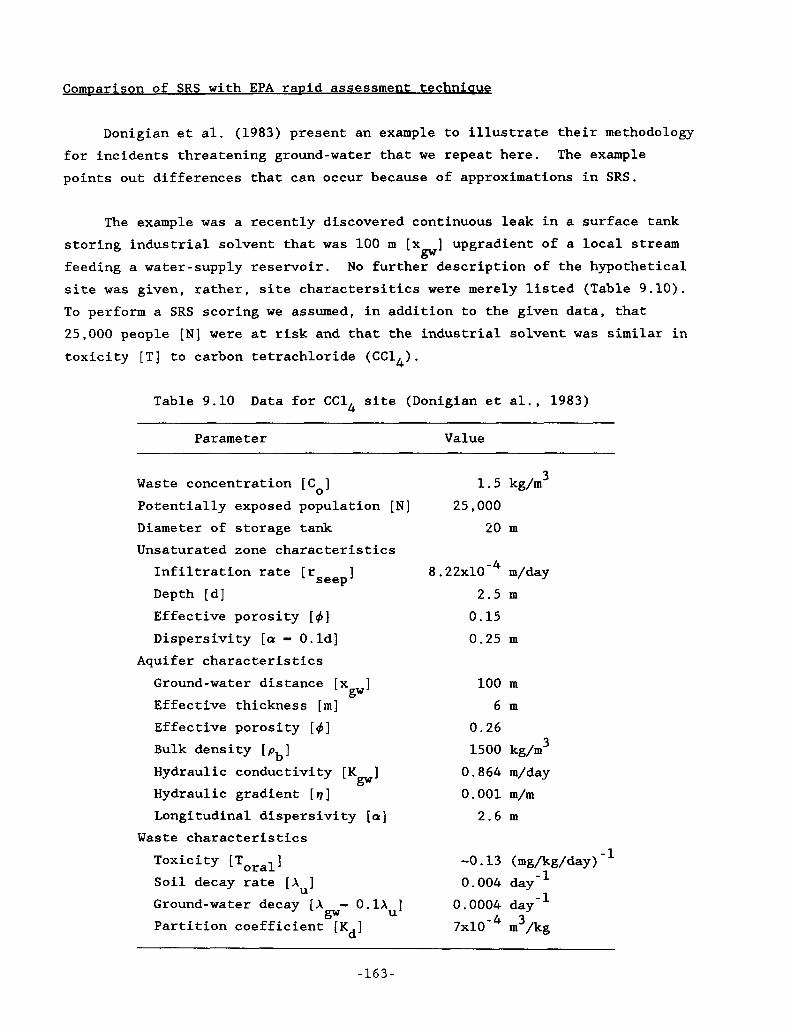
ComDarison of SRS with EPA rapid assessment techniaue
Donigian et al. (1983) present an example to illustrate their methodology for incidents threatening ground-water that we repeat here. The example points out differences that can occur because of approximations in SRS.
The example was a recently discovered continuous leak in a surface tank storing industrial solvent that was 100 m [x ] upgradient of a local stream feeding a water-supply reservoir. No further description of the hypothetical site was given, rather, site charactersitics were merely listed (Table 9.10). To perform a SRS scoring we assumed, in addition to the given data, that 25,000 people [N] were at risk and that the industrial solvent was similar in toxicity [TI to carbon tetrachloride (CCl,).
gw
Table 9.10 Data for CC14 site (Donigian et al., 1983)
Parameter Value
3 Waste concentration [C 3 1.5 kg/m Potentially exposed population [N] 25,000
0
Diameter of storage tank Unsaturated zone characteristics
Infiltration rate [r ] Depth [d] Effective porosity [ d ] Dispersivity [a - O.ld]
seep
Aquifer characteristics Ground-water distance [x ]
Effective thickness [m] Effective porosity [ d ] Bulk density [p,] Hydraulic conductivity [K ]
Hydraulic gradient [ q ]
Longitudinal dispersivity [a]
gw
gw
Waste characteristics Toxicity [Torall Soil decay rate [ A ]
U
20 m
8.22~lO-~ m/day 2.5 m 0.15 0.25 m
100 m 6 m
0.26 1500 kg/m3 0.864 m/day 0.001 m/m 2.6 m
-0.13 (mg/kg/day) -' 0.004 day-'
Ground-water decay [ A - O.lAu] 0.0004 day-' Partition coefficient [K d ] ~ x I O - ~ m3/kg
gw
-163-
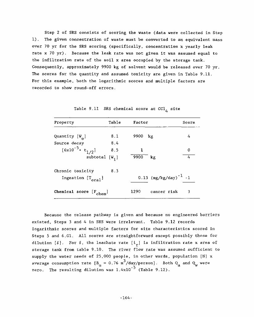
Step 2 of SRS consists of scoring the waste (data were collected in Step The given concentration of waste must be converted to an equivalent mass 1).
over 70 yr for the SRS scoring (specifically, concentration x yearly leak rate x 70 yr). the infiltration rate of the soil x area occupied by the storage tank. Consequently, approximately 9900 kg of solvent would be released over 70 yr. The scores for the quantity and assumed toxicity are given in Table 9.11. For this example, both the logarithmic scores and multiple factors are recorded to show round-off errors.
Because the leak rate was not given it was assumed equal to
Table 9.11 SRS chemical score at CCl& site
Property Table Factor Score
Quantity [W ] 8.1 9900 kg 4 0
Source decay 8.4 [ 6 ~ 1 0 - ~ tl/2] 8.5 1 0
subtotal [Wi] 9900 kg 4
Chronic toxicity 8.3 Ingestion [Torall 0.13 (mg/kg/day) - 1
Chemical score [Fchem] 1290 cancer risk 3
Because the release pathway is given and because no engineered barriers existed, Steps 3 and 4 in SRS were irrelevant. Table 9.12 records logarithmic scores and multiple factors for site characteristics scored in Steps 5 and 6.G1. All scores are straightforward except possibly those for dilution [SI. For 6, the leachate rate [i 3 is infiltration rate x area of
storage tank from table 9.10. The river flow rate was assumed sufficient to supply the water needs of 25,000 people, in other words, population [N] x average consumption rate [B = 0.76 m /day/person]. zero.
r
3 Both Qa and % were U
The resulting dilution was ~ . ~ x I O - ~ (Table 9.12).
-164-
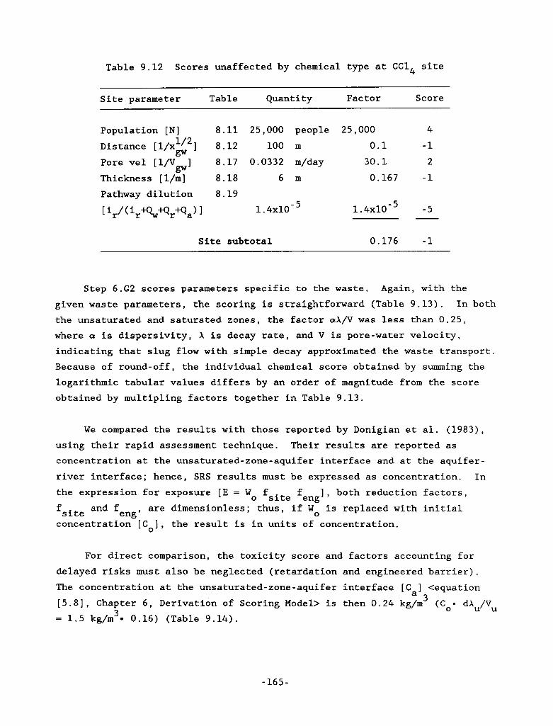
c
I_
L
Table 9.12 Scores unaffected by chemical type at CC14 site
Site parameter Table Quantity Factor Score
Population [N] 8.11 25,000 people 25,000 4
Pore vel [1/V J 8.17 0.0332 m/day 30.1. 2 Thickness [ l/m J 8.18 6 m 0.167 -1
Distance [l/x 'I2] 8.12 100 m 0.1 -1 gw gw
Pathway dilution 8.19 [i,/(i,~+Q,+Q,>l 1.4~10- 1.4~10-~ -5
Site subtotal 0.176 -1
Step 6.G2 scores parameters specific to the waste. Again, with the given waste parameters, the scoring is straightforward (Table 9.13). In both the unsaturated and saturated zones, the factor aX/V was less than 0.25, where Q is dispersivity, X is decay rate, and V is pore-water velocity, indicating that slug flow with simple decay approximated the waste transport. Because of round-off, the individual chemical score obtained by summing the logarithmic tabular values differs by an order of magnitude from the score obtained by multipling factors together in Table 9.13.
We compared the results with those reported by Donigian et al. (1983), using their rapid assessment technique. Their results are reported as concentration at the unsaturated-zone-aquifer interface and at the aquifer- river interface; hence, SRS results must be expressed as concentration. In the expression for exposure [E = W
fsite and feng' concentration [C 1 , the result is in units of concentration.
f J , both reduction factors, o fsite eng are dimensionless; thus, if Wo is replaced with initial
0
For direct comparison, the toxicity score and factors accounting for delayed risks must also be neglected (retardation and engineered barrier). The concentration at the unsaturated-zone-aquifer interface [C J <equation [5.8], Chapter 6, Derivation of Scoring Model> is then 0.24 kg/m = 1.5 kg/m 0.16) (Table 9.14).
a 3 (Coo dXU/VU
3
-165-
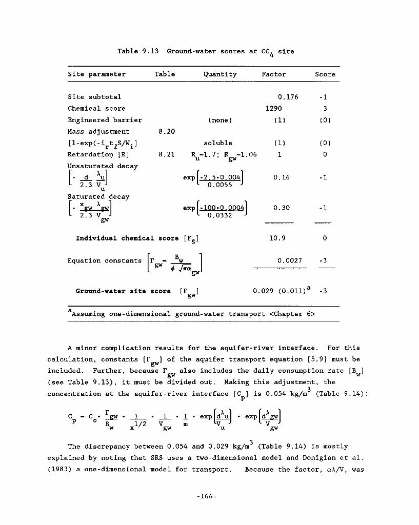
Table 9.13 Ground-water scores at CC4 site
Site parameter Table Quantity Factor Score
Site subtotal Chemical score Engineered barrier Mass adjustment 8.20 [ 1-exp( -irtmS/wi] Retardation [R] 8.21 Unsaturated decav
-I
[- d L] 2.3 Vu
Saturated decay
2.3 V gw
0.176 1290
(none 1 ( 1 1
soluble ( 1 1 Ru=1.7; R -1.06 1
gw
exp [ -2.5.0.004] 0.16 0.0055
exp [ - 100*0.0004] 0.30 0.0332
-1 3
(0)
-1
-1
Individual chemical score [ F S ] 10.9 0
E quat i on constants [..-- 0.0027 - 3
Ground-water site score [FP] 0.029 (O.O1l)a - 3
a Assuming one-dimensional ground-water transport <Chapter 6>
A minor complication results for the aquifer-river interface. For this calculation, constants [I' ] of the aquifer transport equation [5.9] must be included. Further, because r (see Table 9.13), it must be divided out. Making this adjustment, the concentration at the aquifer-river interface [C ] is 0.054 kg/m (Table 9.14):
gw also includes the daily consumption rate [Bw]
gw
3 P
3 The discrepancy between 0.054 and 0.029 kg/m (Table 9.14) is mostly explained by noting that SRS uses a two-dimensional model and Donigian et al. (1983) a one-dimensional model for transport. Because the factor, ( rX /V, was
-166-
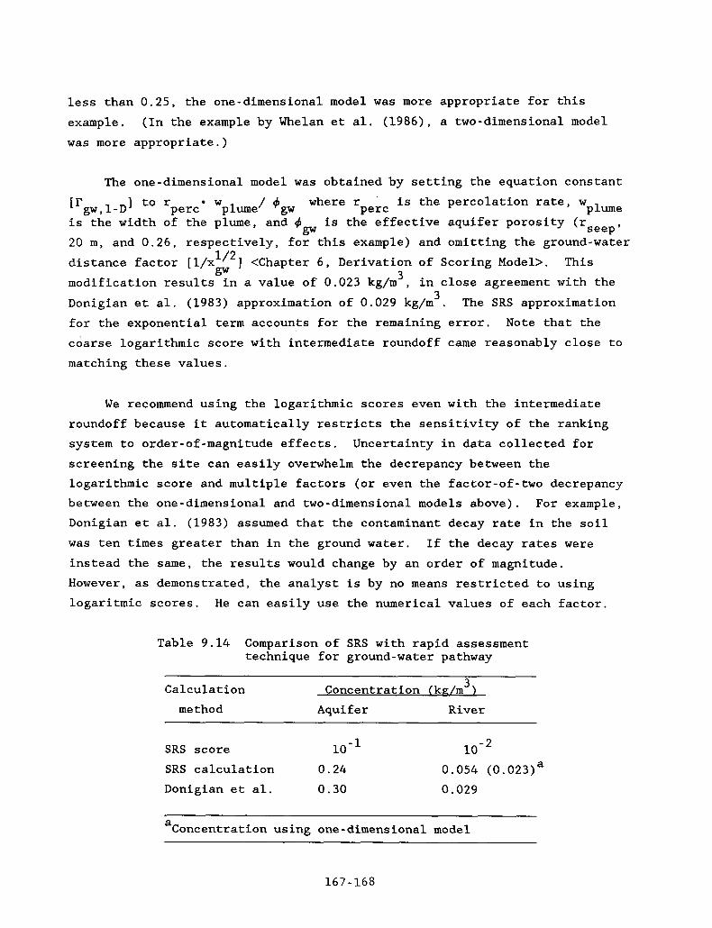
less than 0.25, the one-dimensional model was more appropriate for this example. (In the example by Whelan et al. (1986), a two-dimensional model was more appropriate.)
The one-dimensional model was obtained by setting the equation constant ‘ W is the percolation rate, w Irgw, 1-D 1 to rperc plume/ dgw where ‘perc p lume
seep ’ is the width of the plume, and 4 is the effective aquifer porosity (r gw
20 m, and 0.26, respectively, for this example) and omitting the ground-water distance factor [ l/~l’~] <Chapter 6, Derivation of Scoring Model>. modification results in a value of 0.023 kg/m , in close agreement with the Donigian et al. (1983) approximation of 0.029 kg/m . The SRS approximation for the exponential term accounts for the remaining error. Note that the coarse logarithmic score with intermediate roundoff came reasonably close to matching these values.
This gw 3
3
We recommend using the logarithmic scores even with the intermediate roundoff because it automatically restricts the sensitivity of the ranking system to order-of-magnitude effects. Uncertainty in data collected for screening the site can easily overwhelm the decrepancy between the logarithmic score and multiple factors (or even the factor-of-two decrepancy between the one-dimensional and two-dimensional models above). For example, Donigian et al. (1983) assumed that the contaminant decay rate in the soil was ten times greater than in the ground water. If the decay rates were instead the same, the results would change by an order of magnitude. However, as demonstrated, the analyst is by no means restricted to using logaritmic scores. He can easily use the numerical values of each factor.
Table 9.14 Comparison of SRS with rapid assessment technique for ground-water pathway
3 Calculation Concentration (kdm method Aquifer River
SRS score 10-1 SRS calculation 0.24 0.054 (0.023)a Donigian et al. 0.30 0.029
a Concentration using one-dimensional model
167-168
10. APPENDIX A
SRS Worksheets
Appendix A presents sample worksheets useful for organizing and recording data for the site ranking system (SRS). They can help both in performing the scoring and in documenting the reasons for the assigned score should an audit or reevaluation be necessary.
- 169 -
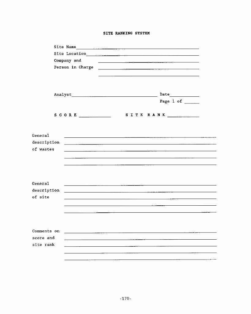
SITE RANKING SYSTEM
Site Name Site Location Company and Person in Charge
Analyst Date
Page 1 of
S C O R E S I T E R A N K
General description of wastes
General description of site
Comments on score and site rank
-170-
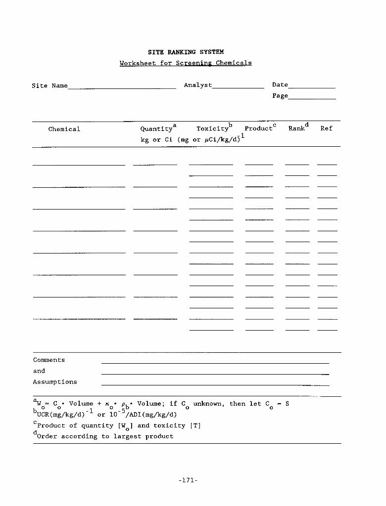
-- SITE RANKING SYSTEM
Worksheet for Screening Chemicals
L
Site Name Analyst Date Page
Chemical Quanti tya Toxicityb ProductC Rankd Ref -1 kg or Ci (mg or pCi/kg/d)
Comments and Assumptions
Volume; if C unknown, then let Co = S 0
“wo- c o o Volume + ,c
bUCR(mg/kg/d) or 10- /AD1 (mg/kg/d) o gb
Product of quantity [Wo] and toxicity [TI C 2 U Order according to largest product
-171-
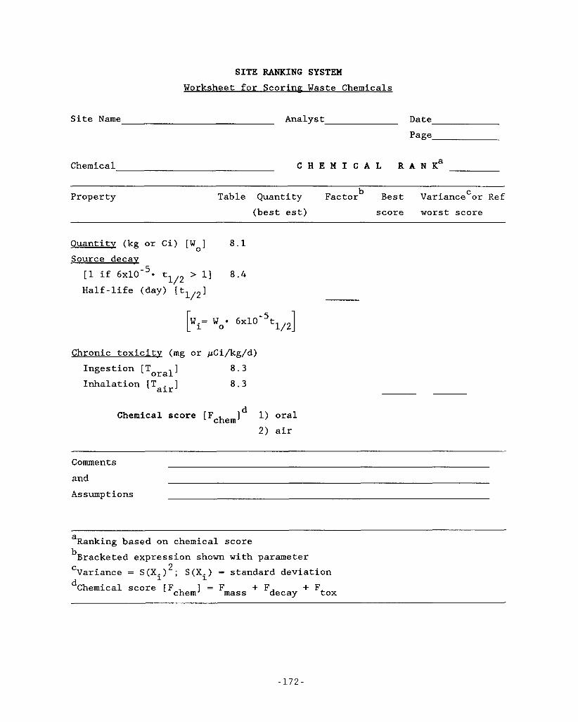
SITE RANKING SYSTEM Worksheet for Scoring Waste Chemicals
Site Name Analyst Date Page
Chemical C H E M I C A L R A N K a
Property Table Quantity Factor Best VarianceCor Ref (best est) score worst score
Ouantitv (kg or Ci) [Wo] 8.1 Source decay
[l if 6 ~ 1 0 - ~ * tl12 > 11 8.4 Half-life (day) [tl12]
1/2 W 6x10 t
1 0 - 5 1 Chronic toxicity (mg or pCi/kg/d) Ingestion [T ] 8.3 oral Inhalation [Tair] 8.3
Chemical score [Fchemld 1) oral 2) air
Comments and Assumptions
Ranking based on chemical score a
bBracketed expression shown with parameter Variance = S ( X . ) * ; S ( X . ) = standard deviation
dChemical score [Fchem] = F mass + Fdecay + Ftox
C 1 1
- 1 7 2 -
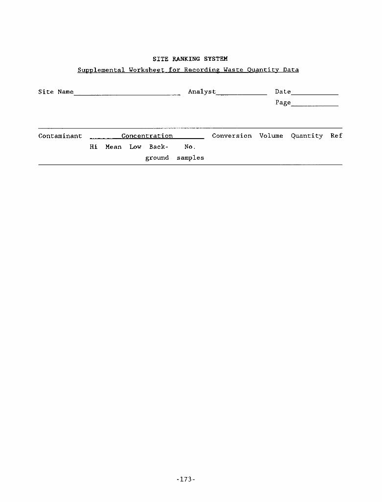
SITE RANKING SYSTEM SuDDlemental Worksheet for Recording - Waste Quantitv Data
Site Name Analyst Date
Page
Contaminant Concentration Conversion Volume Quantity Ref
Hi Mean Low Back- No.
ground samples
-173-
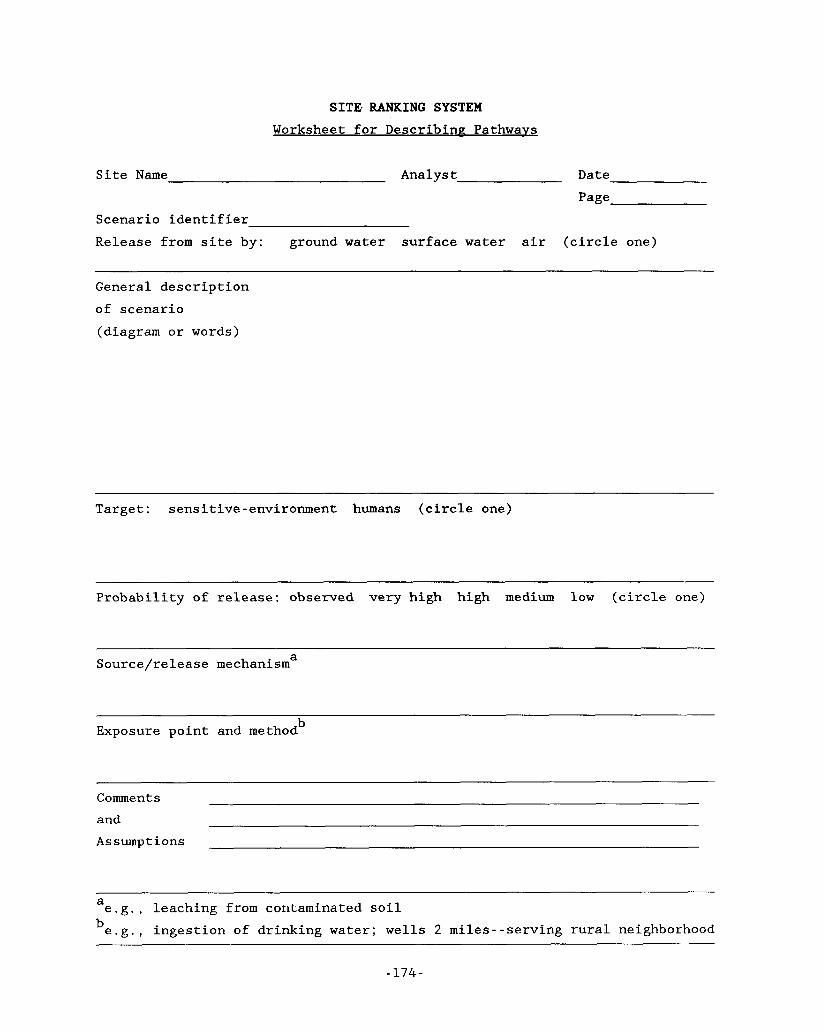
SITE- RANKING SYSTEM Worksheet for Describing Pathways
Site Name Analyst Date Page
Scenario identifier Release from site by: ground water surface water air (circle one)
General description of scenario (diagram or words)
~~ ~~
Target: sensitive-environment humans (circle one)
Probability of release: observed very high high medium low (circle one)
a Source/release mechanism
~~ ~
b Exposure point and method
Comments and Assumptions
a b e.g., leaching from contaminated soil e.g., ingestion of drinking water; wells 2 miles--serving rural neighborhood
- 174-
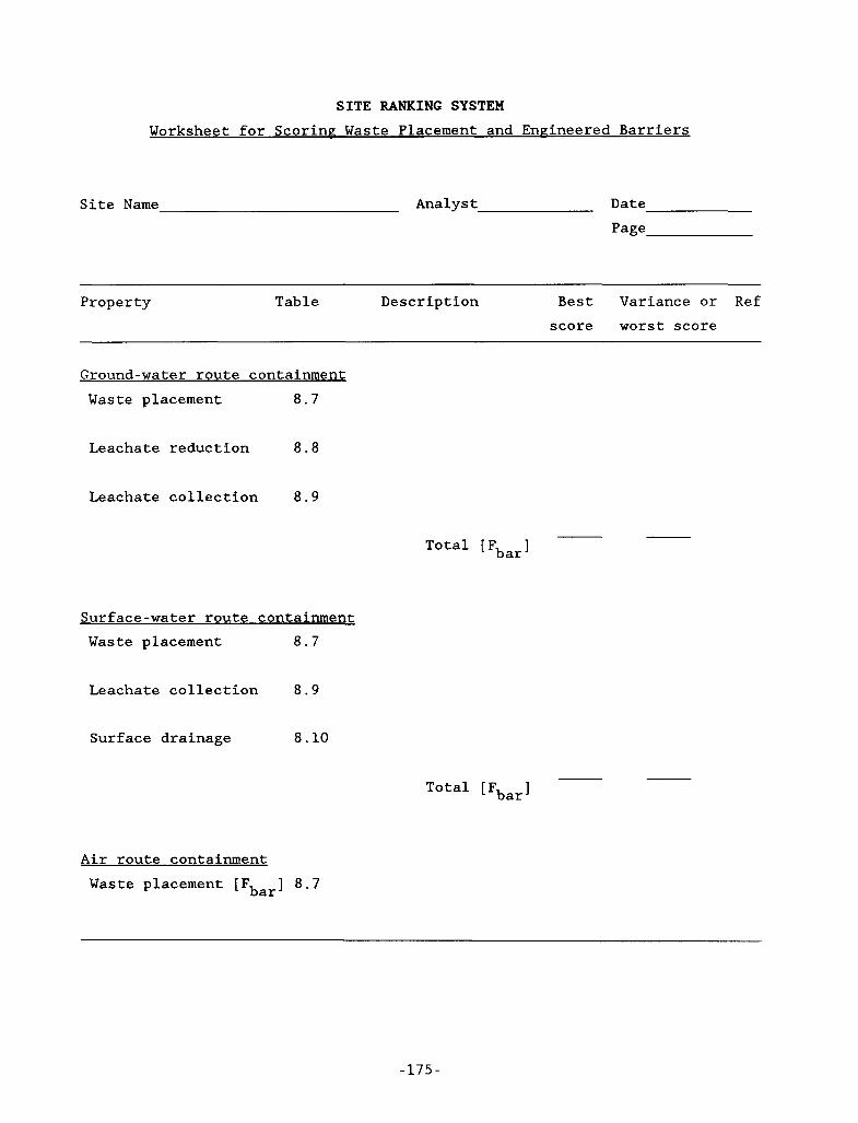
SITE RANKING SYSTEM
Worksheet for Scoring: Waste Placement and EnFineered Barriers
Site Name Analyst Date Page
Property Table Description Best Variance or Ref score worst score
Ground-water route containment
Waste placement 8.7
Leachate reduction 8.8
Leachate collection 8.9
J
Waste placement 8.7
Leachate collection 8.9
Surface drainage 8.10
.- Air route containment
Waste placement [Fbar] 8.7
-175-
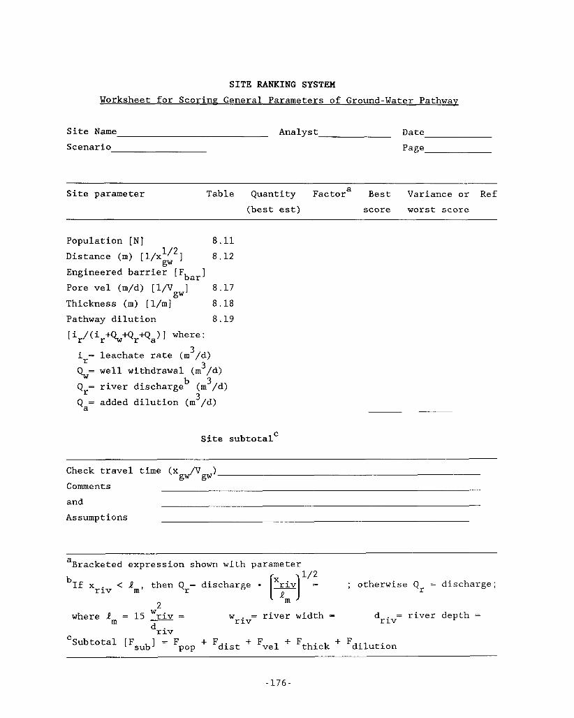
SITE RANKING SYSTEM Worksheet for Scoring General Parameters of Ground-Water Pathway
Site Name Analyst Date Scenario Page
Site parameter Table Quantity Factora Best Variance or Ref (best est) score worst score
Population [N] 8.11 Distance (m) [l/x 1/2 ] 8.12
gw Engineered barrier [Fbar] Pore vel (m/d) [l/V ] 8.17 Thickness (m) [l/m] 8.18 Pathway dilution 8.19
[i,/(ir%+Qr+Qa>l where:
3
gw
3 i = leachate rate (m /d) Qw= well withdrawal (m /d) Qr= river discharge (m3/d) Qa= added dilution (m /d)
r
b 3
Site subtotal'
Check travel time (x /V )
Comments and Assumptions
gw gw
~~
a
b If Xriv < Rm, then Q r = discharge r?] =
Bracketed expression shown with parameter
; otherwise Qr = discharge; 1 / 2
9
= river depth = dr iv where Rm = 15 riv =
dr iv Subtotal [Fsub] = F pop + Fdist + Fvel + Fthick -t Fdilution
w = river width = W L
r iv C
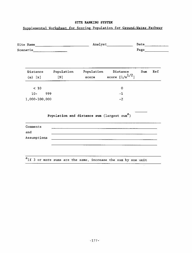
c ”^
c
c
SITE RANKING SYSTEM
Supplemental Worksheet for Scoring PoDulation for Ground-Water Pathway
Site Name Analyst Date
Scenario Page
Distance Population Population D i s tance Sum Ref
(m) [XI [NI score score [l/x 1/2 ]
c 10 10 - 999
1,000-100,000
0
-1 - 2
Population and distance sum (largest suma)
,- Comments and Assumptions
a If 3 or more sums are the same, increase the sum by one unit
- 1 7 7 -
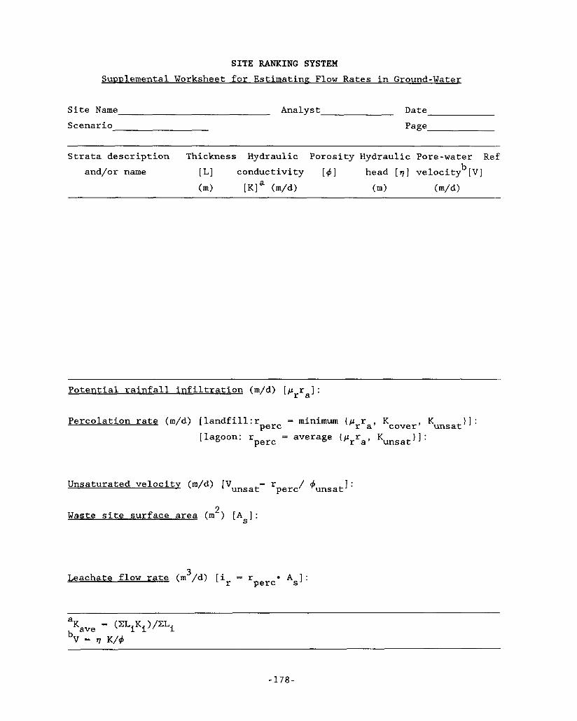
SITE RANKING SYSTEM SupDlemental Worksheet for Estimatina Flow Rates in Ground-Water
Site Name Analyst Date Scenario Page
Strata description Thickness Hydraulic Porosity Hydraulic Pore-water Ref and/or name [L] conductivity [ d ] head [s] velocity [VI b
(m) [KIa (Wd) (m> (m/d)
~ ~~ ~~ ~ ~ ~ ~
Potential rainfall infiltration (m/d) [prra]:
Percolation rate (m/d) [landfill:r perc - minimum {prra, Kcover Kunsat 1 1 : [lagoon: r = average (prra, Kunsatl 1 : perc
Unsaturated velocity (m/d) [Vunsat= rperc/ dunsat I :
2 Waste site surface area (m ) [A 1 : S
As]: 3 perc Leachate flow rate (m /d) [ir = r
a Kave = (XLiKi>/XLi
v = ?I K/d b
-178-
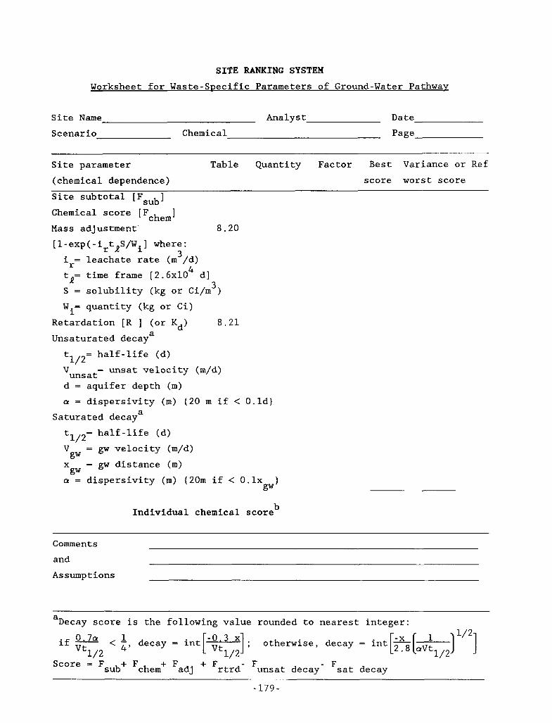
c
.-
SITE RANKING SYSTEM Worksheet for Waste-Specific Parameters of Ground-Water Pathwav
Site Name Analyst Date Scenario Chemical Page
Site parameter Table Quantity Factor Best Variance or Ref (chemical dependence) score worst score
Site subtotal [Fsub] Chemical score [F ] chem Mass adjustment 8.20 [l-exp(-irtRS/Wi] where:
3 i = leachate rate (m /d) t = time frame [2.6x10 d] S = solubility (kg or Ci/m )
W.= quantity (kg or Ci)
4 r R 3
1 8 . 2 1 Retardation [R ] (or Kd)
Unsaturated decaya half-life (d) 5/2=
'unsat= d = aquifer depth (m) a = dispersivity (m) (
unsat velocity
Saturated decaya half-life (d) 5/2=
O m i f <
V = gw velocity (m/d) x = gw distance (m) a = dispersivity (m) (20m if < 0 . 1 ~ )
b
gw gw
gw
Individual chemical score
Comments and Assumptions
a Decay score is the following value rounded to nearest integer:
; otherwise, decay = int 1 4' if 0.7a < - decay = int
1/2 Vt
Fsub+ Fchem+ Fadj + Frtrd- Funsat decay- Fsat decay Score =
-179-
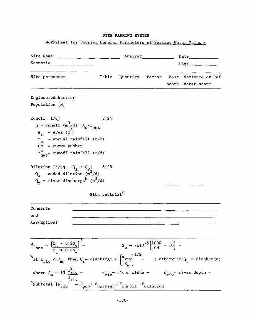
SITE RANKING SYSTEM Worksheet for Scoring General Parameters of Surface-Water Pathway
Site Name Analyst Date Scenario Page
Site parameter Table Quantity Factor Best Variance or Ref score worst score
Engineered barrier Population [N]
Runoff [ l/q] 8.24
2 As - area (m )
r = annual rainfall (m/d) CN = curve number r - runoff rainfall (m/d)
3 q = runoff (m /d) [Asor ] net
a
a net-
Dilution [q / (q + Qa + Qr] 3
8.25 Qa = added dilution (m /d) Qr = river dischargeb (m /d) 3
Site subtotal'
Comments and Assumptions
2 a r
b
= p a - o.2sw] - - r + 0.8Sw
Sw = 7~10-~[% - 101 = net
; otherwise Q = discharge; r 1/2
a If Xriv < Rm, then Q r = discharge r?] =
9
where R = 15 W L riv =
[Fsubl
w = river width = driv= river depth = m r iv dr iv
C
= Fpop+ Fbarrier+ Frunoff+ Fdilution
- 180 -
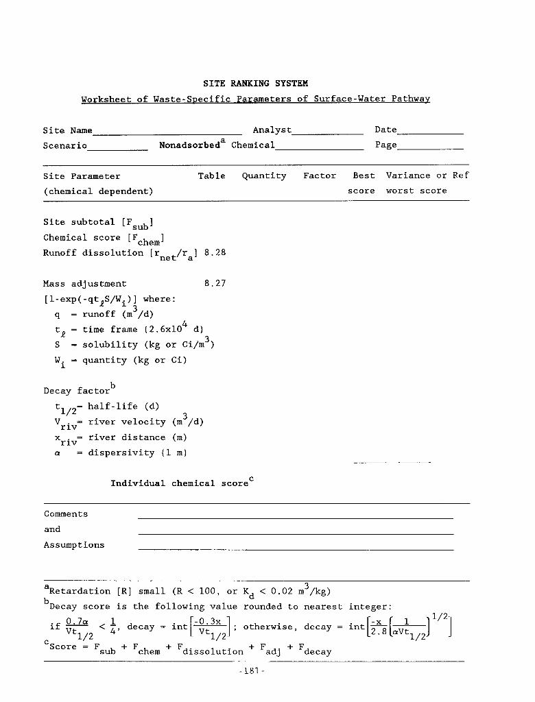
c
c
c
SITE RANKING SYSTEM Worksheet of Waste-Specific Parameters of Surface-Water Pathway
Site Name Analyst Date Scenario Nonadsorbeda Chemical Page
Site Parameter Table Quantity Factor Best Variance or Ref (chemical dependent) score worst score
Site subtotal [Fsub] Chemical score [Fchem] Runoff dissolution [rnet/ra] 8 . 2 8
Mass adjustment 8.27 [l-exp(-qtRS/Wi)] where:
3 q = runoff (m /d) tR = time frame ( 2 . 6 ~ 1 0 ~ d) S = solubility (kg or Ci/m )
W. = quantity (kg or Ci)
3
1
b Decay factor
5/2= 'r iv= r iv
a =
x =
half-life (d) 3 river velocity (m /d)
river distance (m) dispersivity (1 m)
Individual chemical scoreC
Comments and As sump t ions
3 Retardation [R] small (R < 100, or Kd < 0.02 m /kg) a
bDecay score is the following value rounded to nearest integer:
if 0.7a < -, 4 1 decay = int [-:.:;,I ; otherwise, decay = int 1/2
Vt n L
Score = F sub i- Fchem i- Fdissolution -k Fadj + Fdecay
-181-
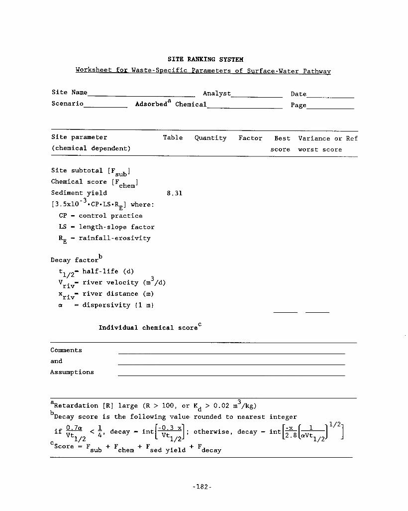
SITE RANKING SYSTEM Worksheet for Waste-SDecific Parameters of Surface-Water Pathway
Site Name Analyst Date Scenario Adsorbeda Chemical Page
Site parameter Table Quantity Factor Best Variance or Ref
(chemical dependent) score worst score
Site subtotal [Fsub] Chemical score [Fchem]
Sediment yield 8.31 [3.5x10q3*CP-LS*R ] where: CP = control practice LS - length-slope factor RE = rainfall-erosivity
E
b Decay factor half-life (d)
5/2= 3 - river velocity (m /d) 'r iv x - river distance (m) r iv a - dispersivity (1 m)
Individual chemical scoreC
Comments and Assumptions
a 3
bDecay score is the following value rounded to nearest integer Retardation [R] large (R > 100, or Kd > 0.02 m /kg)
if - < - 4' 1 decay = int [-:iT11] ; otherwise, decay = int [ix8 - [aVtl/2] 'I2] Vt Score - 1/2 C
Fsub + Fchem + Fsed yield + Fdecay
-182-
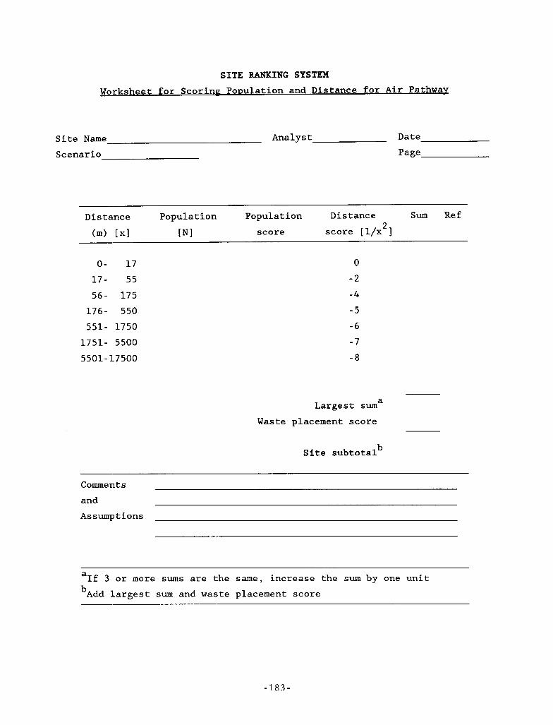
SITE RANKING SYSTEM Worksheet for Scorine Population and Distance for Air Pathway
c-
Site Name Analyst Date Scenario Page
~~
D is t ance Population Population Di s t ance Sum Ref 2 score score [l/x ] (m> [XI [ N I
0- 17
1 7 - 55
56 - 175
1 7 6 - 550
551- 1750
1751- 5500
5501-17500
0
- 2
-4
- 5
- 6
- 7
- a
a Largest sum Waste placement score
b Site subtotal
Comments and Assumptions
a
bAdd largest sum and waste placement score If 3 or more sums are the same, increase the sum by one unit
-183-
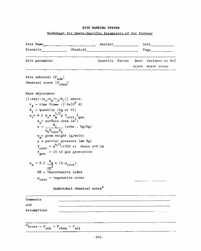
SITE RANKING SYSTEM Worksheet for Waste-Specific Parameters of Air Pathwav
Site Name Analyst Date Scenario Chemical Page
Site parameter Quantity Factor Best Variance or Ref score worst score
Site subtotal [Fsub] Chemical score [Fchem]
Mass adjustment [l-exp(-(ev+ew)t,/Wi)] where:
d) 4 tR = time frame ( 2 . 6 ~ 1 0
W, = quantity (kg or Ci) 1 / 2 f P fcovr, gen
I
e = 0.2 A n w V s m
A = surface area (m') n = 'i (conc., kg/kg)
S
PbdcontAs w = gram weight (g/mole)
p = partial pressure (nun Hg) f f = 10 if gas generation
m
= 4 4 / 3 /(350 s ) where s>O.lm covr
gen
A
PE2 e = 0.2 2 n (l-pcovr) W
PE = Thornthwaite index
pcovr = vegetative cover
Individual chemical scorea
Comments and Assumptions
a sub + Fchem + Fadj Score = F
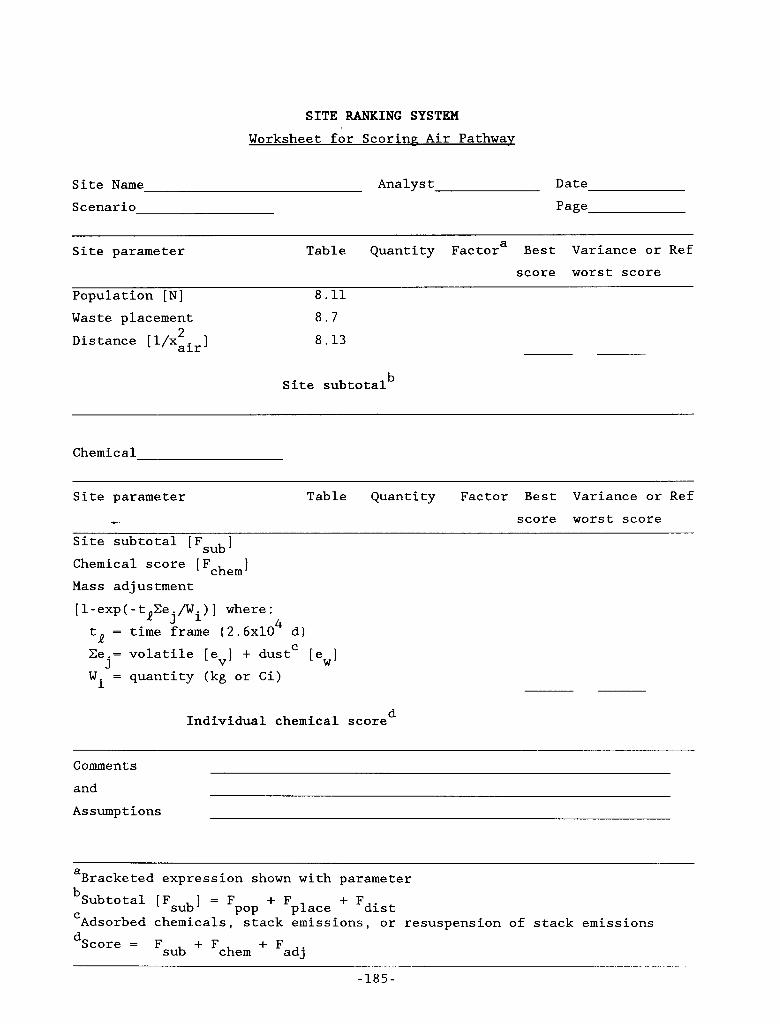
SITE RANKING SYSTEM Worksheet for Scorinp Air Pathway
Site Name Analyst Date
Scenario Page
~~
a Site parameter Table Quantity Factor Best Variance or Ref score worst score
Population [N] 8.11 Waste placement 8.7 Distance [l/xair] 8.13 2
b Site subtotal
Chemical
Site parameter Table Quantity Factor Best Variance or Ref c score worst score
Site subtotal [F ]
Chemical score [Fchem] Mass adjustment [1-exp(-t Ce./Wi)] where:
sub
R J tR = time frame ( 2 . 6 ~ 1 0 ~ d) Ce.= volatile [e ] + dustC [e,] W. = quantity (kg or Ci)
J V
1
d Individual chemical score
c
Comments and Assumptions
a Bracketed expression shown with parameter
pop + Fplace -b Fdist bSubtotal [Fsub] = F C Adsorbed chemicals, stack emissions, or resuspension of stack emissions
dScore = Fsub + Fchem + Fadj - -
- 185 -
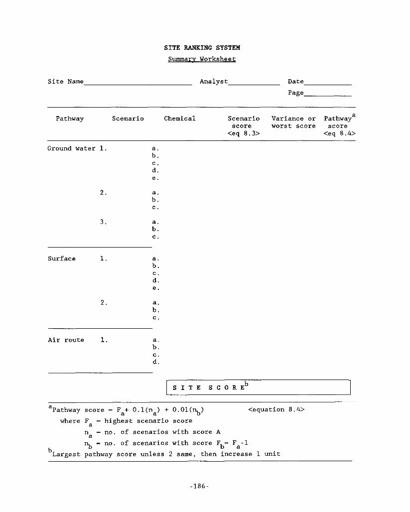
SITE RANKING SYSTEM Summary Worksheet
Site Name Analyst Date Page
Pathway Scenario Chemical Scenario Variance or Pathwaya score worst score score
<eq 8 . 3 > <eq 8 . 4 >
Ground water 1.
2 .
3 .
a. b.
d. e.
C.
a. b. C.
a. b. C.
Surf ace 1.
2.
a. b.
d. e.
C.
a. b. C.
~~
Air route 1. a. b.
d. C.
( S I T E SCORE^ ~ ~~~
Pathway score = Fa+ O.l(na) + O.Ol(n,) a <equation 8 . 4 >
where Fa = highest scenario score n = no. of scenarios with score A rj, = no. of scenarios with score F b a = F -1
bLargest pathway score unless 2 same, then increase 1 unit
a
- 1 8 6 -
SITE RANKING SYSTEM References
Site Name Analyst Date
Page
c
.-
e
Reference
ID
Reference
1 8 7 - 188
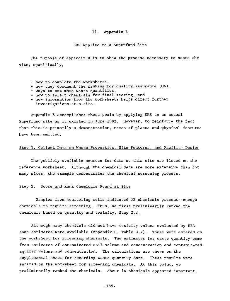
11. Appendix B
SRS Applied to a Superfund Site
c
.-
.-
e
The purpose of Appendix B is to show the process necessary to score the site, specifically,
how to complete the worksheets, how they document the ranking for quality assurance (QA), ways to estimate waste quantities, how to select chemicals for final scoring, and how information from the worksheets helps direct further investigations at a site.
Appendix B accomplishes these goals by applying SRS to an actual Superfund site as it existed in June 1982. However, to reinforce the fact that this is primarily a demonstration, names of places and physical features have been omitted.
Step 1. Collect Data on Waste Properties. Site Features. and Facility Design
The publicly available sources for data at this site are listed on the reference worksheet. many sites, the example demonstrates the chemical screening process.
Although the chemical data are more extensive than for
Step 2. Score and Rank Chemicals Found at Site
Samples from monitoring wells indicated 32 chemicals present--enough chemicals to require screening. Thus, we first preliminarily ranked the chemicals based on quantity and toxicity, Step 2.2.
Although many chemicals did not have toxicity values evaluated by EPA some estimates were available (Appendix C, Table C.7). These were entered on the worksheet for screening chemicals. The estimates for waste quantity came from estimates of contaminated soil volume and concentration and contaminated aquifer volume and concentration. The calculations are shown on the supplemental sheet for recording waste quantity data. These results were entered on the worksheet for screening chemicals. At this point, we preliminarily ranked the chemicals. About 14 chemicals appeared important.
-189-
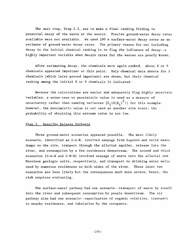
The next step, Step 2 .3 , was to make a final ranking folding in potential decay of the waste at the source. available were not available. We used 100 x surface-water decay rates as an estimate of ground-water decay rates. decay in the initial chemical ranking is to flag the influence of decay--a highly important variable when decays rates for the wastes are poorly known.
Precise ground-water decay rates
The primary reason for not including
After estimating decay, the chemicals were again ranked. About 8 or 9 chemicals appeared important at this point. chemicals (which later proved important) are shown, but their chemical ranking among the initial 8 or 9 chemicals is indicated.
Only chemical data sheets for 5
Because the calculations are easier and adequately flag highly uncertain variables, a worse-case or pessimistic value is used as a measure of uncertainty rather than summing variances [Ci(S(Xi) ) ] for this example. However, the pessimistic value is not used as another site score; the probability of obtaining this extreme value is too low.
2
Step 3 . Describe Release Pathways
Three ground-water scenarios appeared possible. The most likely scenario, identified as G-A-R, involved seepage from lagoons and solid waste dumps on the site, tranport through the alluvial aquifer, release into the river, and consumption by a few residences downstream. The second and third scenarios (G-A-W and G-M-W) involved seepage of waste into the alluvial and Morrison geologic units, respectively, and transport to drinking water wells used by numerous residences on both sides of the river. These later two scenarios are less likely but the consequences much more severe; hence, the risk requires evaluating.
The surface-water pathway had one scenario--transport of waste by runoff into the river and subsequent consumption by people downstream. The air pathway also had one scenario--vaporization of organic volatiles, transport to nearby residences, and inhalation by the occupants.
- 190 -
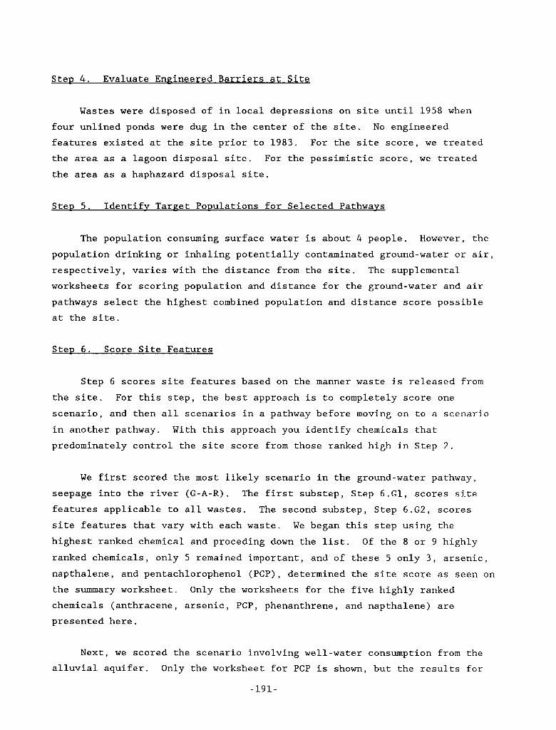
,-
I
Step 4 . Evaluate Engineered - Barriers at Site
Wastes were disposed of in local depressions on site until 1958 when four unlined ponds were dug in the center of the site. No engineered features existed at the site prior to 1983. For the site score, we treated the area as a lagoon disposal site. For the pessimistic score, we treated the area as a haphazard disposal site.
Step 5. Identify Target - Populations for Selected Pathways
The population consuming surface water is about 4 people. However, the population drinking or inhaling potentially contaminated ground-water or air, respectively, varies with the distance from the site. The supplemental worksheets for scoring population and distance for the ground-water and air pathways select the highest combined population and distance score possible at the site.
Step 6. Score Site Features
Step 6 scores site features based on the manner waste is released from the site. For this step, the best approach is to completely score one scenario, and then all scenarios in a pathway before moving on to a scenario in another pathway. With this approach you identify chemicals that predominately control the site score from those ranked high in Step 2.
We first scored the most likely scenario in the ground-water pathway, seepage into the river (G-A-R). The first substep, Step 6.G1, scores site features applicable to all wastes. The second substep, Step 6.G2, scores site features that vary with each waste. We began this step using the highest ranked chemical and proceding down the list. ranked chemicals, only 5 remained important, and of these 5 only 3, arsenic, napthalene, and pentachlorophenol (PCP), determined the site score as seen on the summary worksheet. Only the worksheets for the five highly ranked chemicals (anthracene, arsenic, PCP, phenanthrene, and napthalene) are presented here.
Of the 8 or 9 highly
Next, we scored the scenario involving well-water consumption from the alluvial aquifer. Only the worksheet for PCP is shown, but the results for
-191-
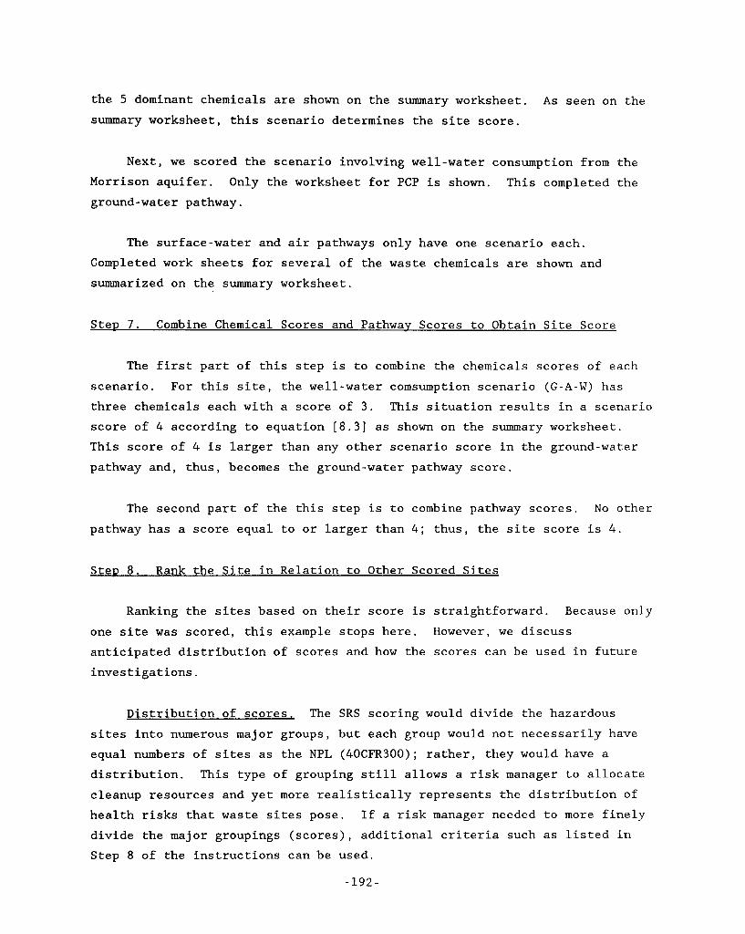
the 5 dominant chemicals are shown on the summary worksheet. summary worksheet, this scenario determines the site score.
A s seen on the
Next, we scored the scenario involving well-water consumption from the Morrison aquifer. Only the worksheet for PCP is shown. This completed the ground-water pathway.
The surface-water and air pathways only have one scenario each. Completed work sheets for several of the waste chemicals are shown and summarized on the summary worksheet.
Step 7. Combine Chemical Scores and Pathway Scores to Obtain Site Score
The first part of this step is to combine the chemicals scores of each scenario. For this site, the well-water cornsumption scenario (G-A-W) has three chemicals each with a score of 3. This situation results in a scenario score of 4 according to equation [8.3] as shown on the summary worksheet. This score of 4 is larger than any other scenario score in the ground-water pathway and, thus, becomes the ground-water pathway score.
The second part of the this step is to combine pathway scores. N o other pathway has a score equal to or larger than 4; thus, the site score is 4 .
Step 8. Rank the Site in Relation to Other Scored Sites
Ranking the sites based on their score is straightforward. Because only
one site was scored, this example stops here. However, we discuss anticipated distribution of scores and how the scores can be used in future investigations.
Distribution of scores. The SRS scoring would divide the hazardous sites into numerous major groups, but each group would not necessarily have equal numbers of sites as the NPL (40CFR300); rather, they would have a distribution. This type of grouping still allows a risk manager to allocate cleanup resources and yet more realistically represents the distribution o f
health risks that waste sites pose. If a risk manager needed to more finely divide the major groupings (scores), additional criteria such as listed in Step 8 of the instructions can be used.
- 1 9 2 -
The distribution of scores depends heavily on the type of sites being scored. SRS has not been extensively tested and so we cannot state the range or distribution of scores. EPA Superfund sites, we surmise CERCLA-type sites would typically score between -10 and + l o , with +15 and -20 encompassing almost all sites. The most probable value would probably lie between +2 and +5.
However, based on a preliminary ranking of five
Further investigations. The results from SRS can be used in two ways:
1. During the site screening, early use of SRS with readily available data can identity important pathways and/or variables. A risk manager can use this information to direct data collection efforts that are still within the scope of site screening yet more costly and/or difficult to obtain (for example, drilling monitoring wells, throughly searching government records on well completions, or requesting information from potentially liable parties).
2. Final results can be used in designing RI/FS studies. Although more detailed data will be collected on all variables and pathways, less resources can be directed toward low risk pathways or unimportant variables at the site.
We can demonstrate these concepts with the example site. First, a minor
Because well use near the site data refinement might occur during screening: was only sketchy, a portion of any remaining resources could be used to identify well use. Second, a more detailed risk assessment may wish to collect data on transport under the river to the numerous wells and collect data on air quality to more carefully assess the hazards from these less likely but more severe consequence scenarios. Third, although air stripping, a common cleanup technique, could successfully remove several organic volatiles at the site, the large air-pathway hazard identified by SRS could help direct RI/FS studies toward alternate cleanup techniques.
- 193 -
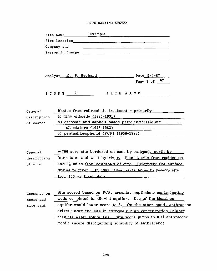
SITE RANKING SYSTEM
Site Name Example
Site Location Company and Person in Charge
Analyst R. P. Rechard Date 5-4-87 Page 1 of 62
S C O R E 4 S I T E R A N K
General description a) zinc chloride (1886-1931)
Wastes from railroad tie treatment - primarily
b) creosote and asphalt-based petroleum /residuum
c) pentachlorophenol (PCP) (1956-1983)
of wastes oil mixture (1928-1983)
General description of site and 13 miles from downtown of citv. Relativelv
- 700 acre site bordered on east by railroad, north by interstate, and west by river. Plant 4 mile from residences
nit0
from 100 pr f h L p h i n
Comments on
score and
Site scored based on PCP, arsenic, napthalene contaminating wells completed in alluvial aquifer. Use of the Morrison
site rank aquifer would lower score to 3. On the other hand, anthracene
than its water solubility). mobile (score disregarding solubility of anthracene)
Sitescore jumps to 8 if anihmmm e
-194-
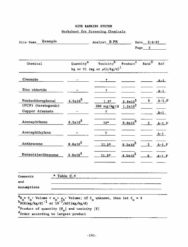
SITE RANKING SYSTEM Worksheet for Screenine. Chemicals
Site Name Analyst R PR Date 5-4-87 Page 2
Chemical Quanti tya Toxicityb Product' Rankd R e f
kg or Ci (mg or pCi/kg/dj' .-
A-l Creosote
Zinc chloride
?
A-l ?
5 A-1, F 4 . 5x10⁵ 1.3* m5 300 mg/kg/d 1 . 2 ~ 1 0 ~
Pen tachlorophenal ( P C P 1 ( teratogenic ) Copper Arsenate ? A-1
6 . 5x10⁵ 6 15* 9.9xlO Acenaphthene 2 A - l , F
Acenaphthylene ? A-1
5 8 . 0 ~ 1 0 11.5* 9.2x105 Anthracene
Benzo(a) anthracene
3 A-1 , F
3 . 9x1o4 11.5*
Comments * Table C.7
and
Assumptions
aWo= c o o Volume + n b
Volume; if Co unknown, then let Co - S o ;bo UCR(mg/kg/d) -' or 10- /ADI(mg/kg/d) Product of quantity [Wo] and toxicity [TI C
dOrder according to largest product
- 195 -
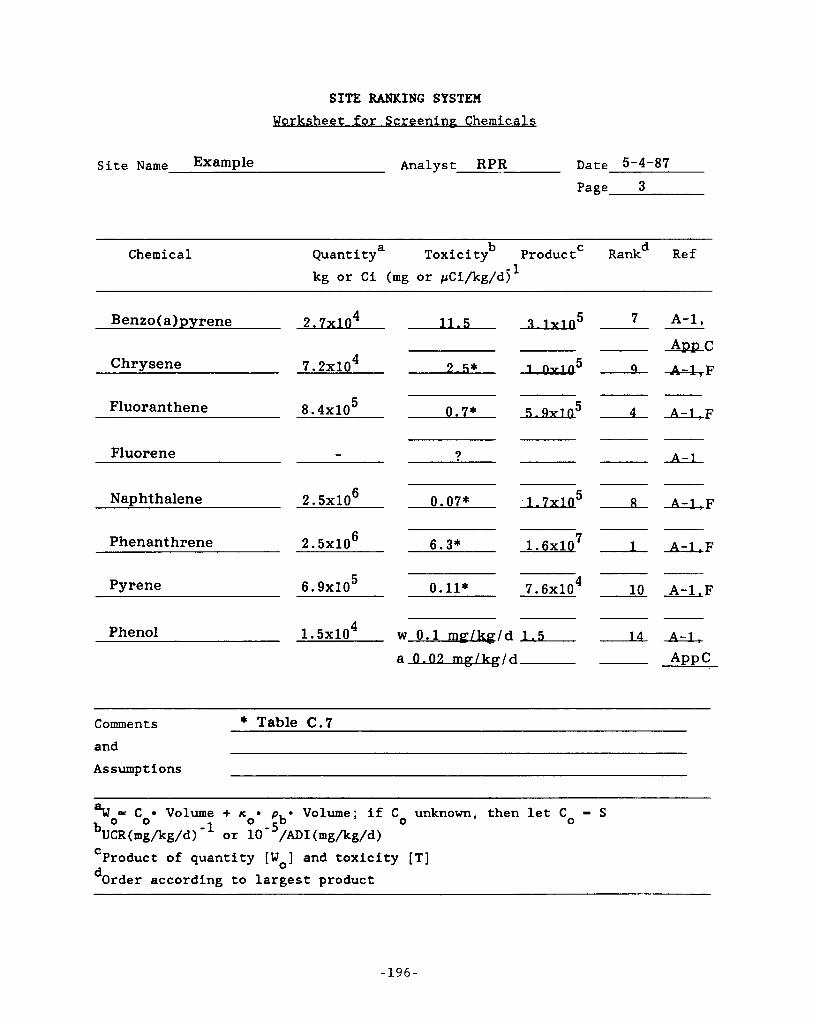
SITE RANKING SYSTEM Worksheet for Screenine Chemicals
Site Name Example Analyst .RPR Date 5-4-87
Page 3
Chemical Quanti tya Toxicityb Product‘ Rankd Ref kg or Ci (mg or pCi/kg/djl
Benzo (alpyrene
Chrvsene
Fluoranthene
Fluorene
NaDhthalene
Phenanthrene
Pyrene
Phenol
11.5 R.1u1n5 4 2 . 7 ~ 1 0
2 s* -l&U5 4 7.2~10
0.7* 5.9x1n5 5 8 . 4 ~ 1 0
? -
2 . 5 ~ 1 0 6 0.07* -5
7 6 . 3 * 1 . 6 ~ 1 0 6 2 . 5 ~ 1 0
4 6 . 9x1O5 0.11* 7 . 6 ~ 1 0
1 . 5 ~ 1 0 w 0 . 1 m g u I d L a 0 . 0 2 ? k g / d
4 A-1.F
8 M P F
2 A - 1 . F
10 A-1,F
2 A - l . - APPC
Comments * Table C.7 and
Assumptions
“w = C Volume + no- gb* Volume; if Co unknown, then let Co = S bUCR(mg/kg/d)-l or 10- /ADI(mg/kg/d)
dOrder according to largest product
0 0
Product of quantity [WJ and toxicity [TI C
- 1 9 6 -
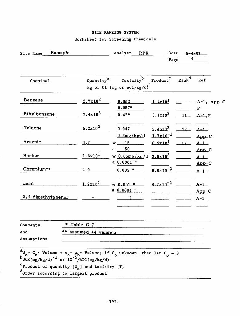
SITE RANKING SYSTEM Worksheet for Screeninv Chemicals
Site Name Example Analyst RPR Date - - Page 4
Chemical Quanti tya Toxicityb Product' Rankd Ref kg or Ci (mg or pCi/kg/dj'
2 . 7x10² 0 .052 L4zln1 A - l . A p p C B e n z e n e
0 .057* F Et h y l b e n z e n e 7 . 4x10³ 0 .42* 3.12103 11-
Toluene 5 . 2x10³ 0 .047 m2 L A - l
A r s e n i c 4 . 7 w 1 5 fi.sxlnl 1 R A - l A W - C
h C
a 0.0001 App-C
0. S m ~ / k g / d 1. 7x10⁻¹
a 50
Barium 1 . 3x101 w 0 . 0 5 m g / k g / d 2 . 5x10³ A-l
4 . 9 0 .005 " 9.8x10⁻³ A-l Chromium * *
w D - n n l 11 8.7x1n-2 A-l a 0 .0004 A D r , C
Lead -01
2 ? 4 dimethylphenol - 3 A-l
Comments * Table C . 7
and ** a s s u m e d +4 valence Assumptions
Volume; if Co unknown, then let Co = S gb aWo= c o o Volume + K O *
bUCR(mg/kg/d) -' or 10- /AD1 (mg/kg/d) Product of quantity [WO] and toxicity [TI C
dOrder according to largest product
-197-
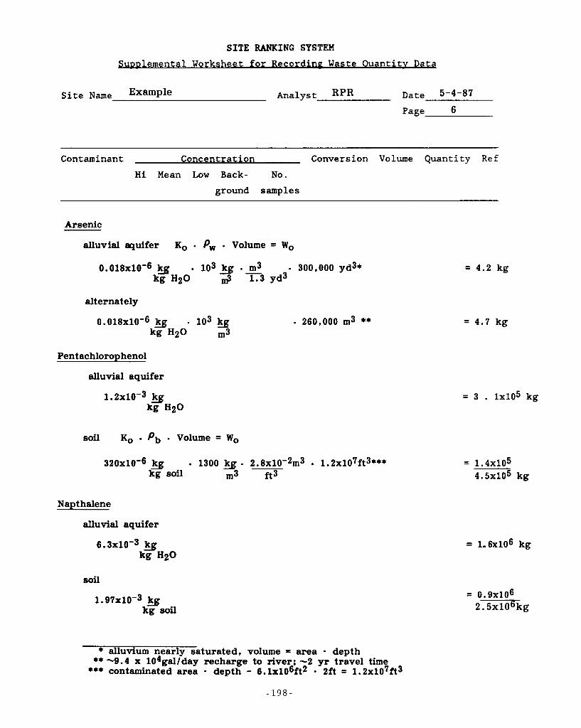
SITE RANKING SYSTEM SuDDlemental Worksheet for Recordine Waste Ouantitv Data
Site Name Analyst RPR Date 5-4-87
Page 6
Contaminant Concentration Conversion Volume Quantity R e f
Hi Mean Low Back- No.
ground samples
Arsenic
alluvial equifer KO Pw - Volume = Wo
0.018~10’6 Q 103 k~ - - m3 . 300,000 yd3* kg H20 1.3 yd3
alternately
0.018~10’6 9 - l o 3 k_g . 260,000 m3 ** kg H 2 0 m3
Pentachlorophenol
alluvial aquifer
1 . 2 ~ 1 0 - 3 9 kg H20
soil K, P, . Volume = W,
320x10’6 9 1300 k~ . 2.8x10⁻²m3 1.2x107ft3*** kg soil m3 f t3
Nap thalene
alluvial aquifer
6 . 3 ~ 1 0 - ~ Q kg H20
1 .97~10-3 Q kg soil
= 4.2 kg
= 4.7 kg
= 3 . 1x10⁵ kg
= 1 . 4 ~ 1 0 5 4 . 5 ~ 1 0 5 kg
= 1 . 6 ~ 1 0 ~ kg
= 0.9x10⁶ 2. 5x10⁶kg
* alluvium nearly saturated, volume = area - dep th ** - 9 . 4 x lOlgal/day recharge to river; -2 yr travel t i m e
*** contaminated area - depth - 6.1x106ft2 - 2ft = 1.2x107ft3
- 1 9 8 -
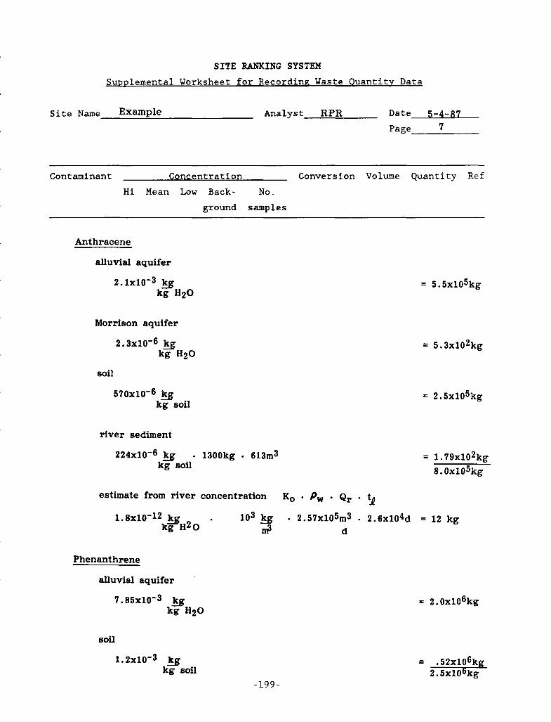
SITE RANKING SYSTEM SuDolemental Worksheet for Recordinn Waste Ouantitv Data
Site Name Example Analyst RPR Date 5-4-87 Page 7
Contaminant Concentration Conversion Volume Quantity R e f
Hi Mean Low Back- No. ground samples
Anthracene
alluvial aquifer
2.1~10-3 9 kg H20
Morrison aquifer
2.3~10-6 & kg H20
soil
510x10-6 & kg soil
river sediment
224x10’6 & . 1300kg - 613m3 kg soil
= 5.5x10⁵kg
= 5.3x10²kg
= 2.5x10⁵kg
= 1.79x10²kg 8.0x10⁵kg
estimate from river concentration KO Pw Qr fa 1.8~10-12 & . lo3 & . 2.57x10⁵m3 . 2.6x10⁴d = 12 kg
kg H20 ll? d
Phenanthrene
alluvial aquifer
soil
1.2~10-3 9 kg soil
= 2.0x10⁶kg
= .52xl;6kg 2.5~10 kg
-199-
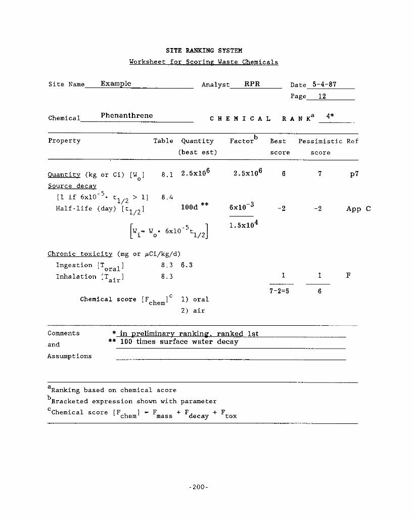
SITE RANKING SYSTEM Worksheet for Scoring Waste Chemicals
Site Name Example Analyst RPR Date 5-4-87 Page 12
Chemical Phenanthrene C H E M I C A L R A N K a 4*
Property Table Quantity Factorb Best Pessimistic Ref (best est) score score
Quantity (kg or Ci) [Wo] 8.1 2 . 5 ~ 1 0 ~
Source decay
2. 5x10⁶
[l if 6 ~ 1 0 - ~ - t1,2 > 11 Half-life (day) [t, ,,,I lOOd ** 6 ~ 1 0 - ~
8 . 4
1. 5x10⁴ 1 / 2
W.= W 6x10 t 1 0 - 5 1
Chronic toxicity (mg or pCi/kg/d) Ingestion [T 3 8.3 6.3 oral Inhalation [Tair] 8.3
Chemical score [FchemIc 1) oral 2) air
7 P7
-2
1 1
7 -2=5 6 -~
F
Comments * in preliminary ranking., ranked 1st and Assumptions
** 100 times surface water decay
a
bBracketed expression shown with parameter Ranking based on chemical score
C mass + Fdecay + Ftox Chemical score [F 3 = F chem
- 200 -
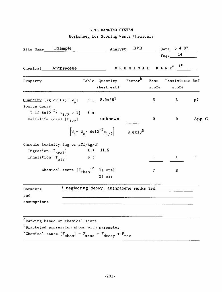
SITE RANKING SYSTEM Worksheet for Scoring - Waste Chemicals
Site Name Analyst RPR Date 5-4-87
Page 14
1* Chemical Anthracene C H E M I C A L R A N K a
Property Table Quantity Factor Best Pessimistic Ref (best est) score score
Quantity (kg or Ci) [Wo] 8.1 8 . 0 ~ 1 0 ~ Source decay
- 5 [l if 6x10 t1/2 > 13 8.4 Half-life (day) [tlI2] unknown
- 5 ] 8 . 0 ~ 1 0 ~ W.= W 6x10 t 1/2 1 0
Chronic toxicity (mg or pCi/kg/d)
oral Inhalation [Tair] 8.3
Ingestion [T 3 8.3 11.5
Chemical score [FchemJc 1) oral 2) air
6
0
6
0
P7
1 1 F
7 8
Comments * neglecting decay, anthracene ranks 3rd
and Assumptions
a
bBracketed expression shown with parameter Ranking based on chemical score
C mass + Fdecay + Ftox Chemical score [Fchem] = F
-201-
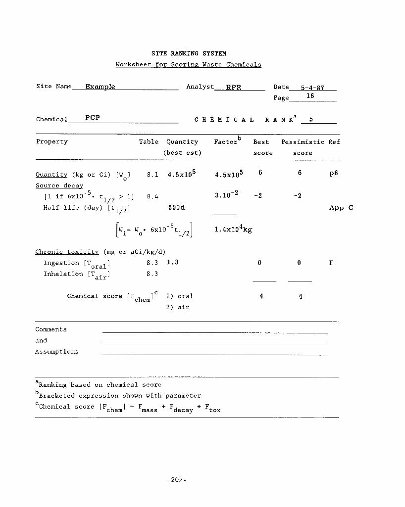
SITE RANKING SYSTEM Worksheet for Scorinv Waste Chemicals
Site Name Example Analyst RPR Date - - Page 16
Chemical P c P C H E M I C A L R A N K a 5
Property Table Quantity Factorb Best Pessimistic Ref (best est) score score
Ouantity (kg or Ci) [Wo] 8.1 4 . 5 ~ 1 0 ~ 4 . 5 ~ 1 0 ~ 6
Source decay [l if 6x10 -5 tl12 > 11 8 . 4 3.10-2 -2
Half-life (day) [tl12] 500d
1 /2 W.= W 6x10 t 1 0 - 5 1
Chronic toxicity (mg or pCi/kg/d) Ingestion [T ] 8.3 1 . 3 oral Inhalation [Tair] 8 . 3
Chemical score [FchemIc 1) oral 2 ) air
1. 4 x 1 0 4 k g
6 P6
-2
0 0
_ _ _ ~
4 4
F
Comments and Assumptions
a
bBracketed expression shown with parameter Ranking based on chemical score
C mass + Fdecay i- Ftox Chemical score [Fchem] = F
- 202 -
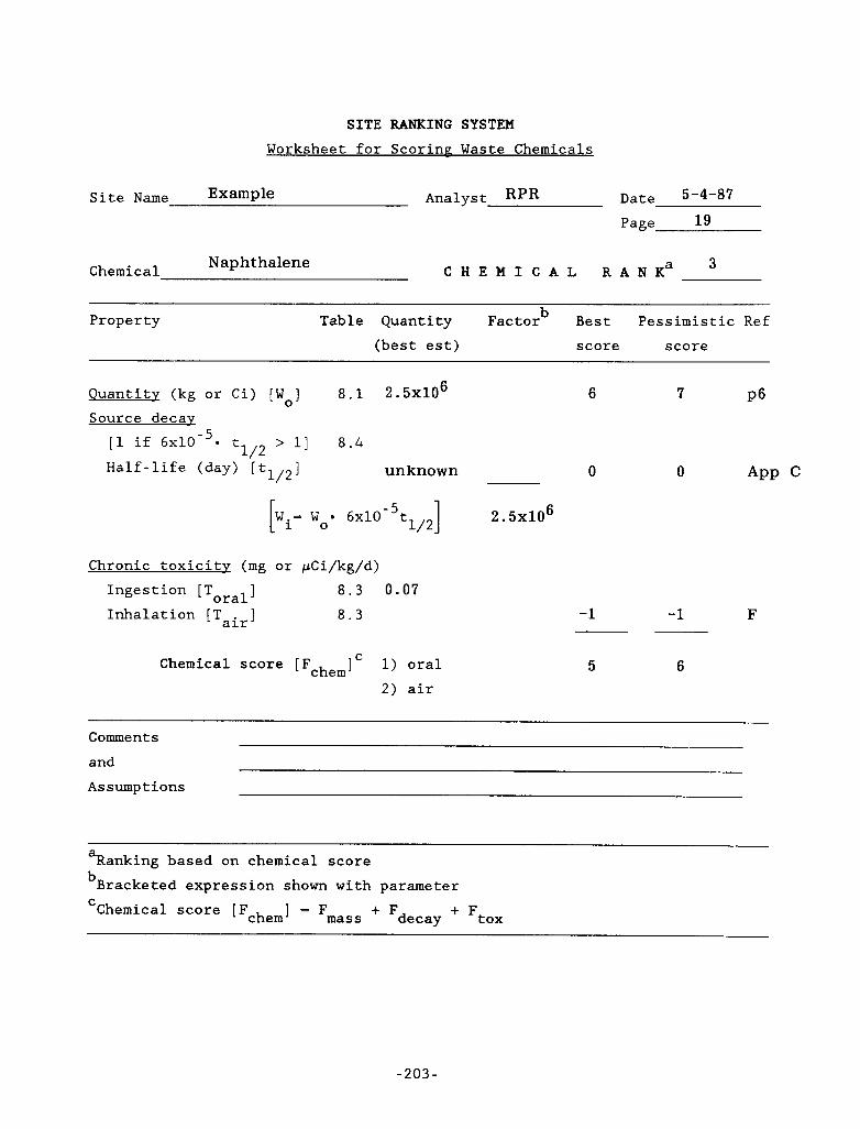
SITE RANKING SYSTEM Worksheet for Scorinz Waste Chemicals
Site Name Analyst RPR Date 5-4-87
3 C H E M I C A L R A N K a Naphthalene Chemical
~~ ~~~
Property Table Quantity Factorb Best Pessimistic Ref (best est) score score
Quantity (kg or Ci) [Wo] 8.1 2 . 5 ~ 1 0 ~ 6 7 P6 Source decav
[l if 6 ~ 1 0 - ~ * tlI2 > 11 8.4
Half-life (day) [tlI2] unknown 0
] 2 . 5 ~ 1 0 ~ 1 / 2
[W,= Woe 6 ~ 1 0 - ~ t L A
Chronic toxicity (mg or Ingestion [T ]
Inhalation [Tair] oral
Chemical score Fchemlc '1 Oral 2) air
0
-1 -1 F
5 6
Comments and Assumptions
a
bBracketed expression shown with parameter Ranking based on chemical score
C mass + Fdecay + Ftox Chemical score [Fchem] = F
-203-
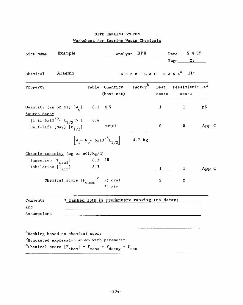
SITE RANKING SYSTEM Worksheet for Scoring - Waste Chemicals
Chemical Arsenic C H E M I C A L R A N K a 11*
Property Table Quantity Factor Best Pessimistic Ref (best est) score score
Quantity (kg or Ci) [Wo] 8 . 1 4.7
Source decay [l if 6 ~ 1 0 - ~ * tlI2 > 11 Half-life (day) [tl/2] metal
8 . 4
- 5 ] 4 . 7 kg 1 / 2
W.= W 6x10 t 1 0
Chronic toxicity (mg or pCi/kg/d) Ingestion [T ] 8 . 3 15 oral Inhalation [Tair] 8 . 3
Chemical score [Fchemlc 1) oral 2) air
1
0
1
0
Comments ~~
* ranked 13th in preliminary rankinv (no decay) and Assumptions
a
bBracketed expression shown with parameter Ranking based on chemical score
C mass + Fdecay + Ftox Chemical score [Fchem] = F
-204-
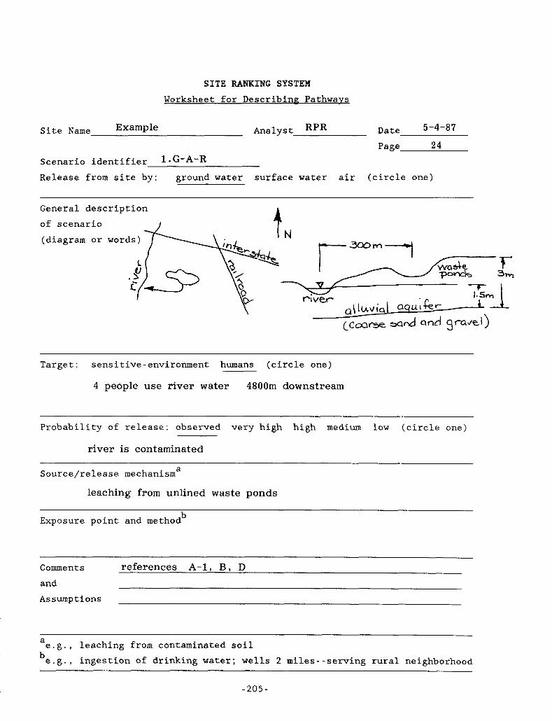
SITE RANKING SYSTEM Worksheet for Describing - Pathwavs
c.
Site Name Analyst RPR Date 5-4-87 Page 2 4
Scenario identifier 1 .G-A-R
Release from site by: ground water surface water air (circle one)
General description
of scenario I
(diagram ,-
A
P
I
or N
Target: sensitive-environment humans (circle one)
4 people use river water 4800m downstream
Probability of release: observed very high high medium low (circle one)
river is contaminated
a Source/release mechanism
leaching f rom unlined waste ponds
b Exposure point and method
Comments references A-1, B , D and Assumptions
~
a
b e.g., leaching from contaminated soil e.g., ingestion of drinking water; wells 2 miles--serving rural neighborhood
-205 -
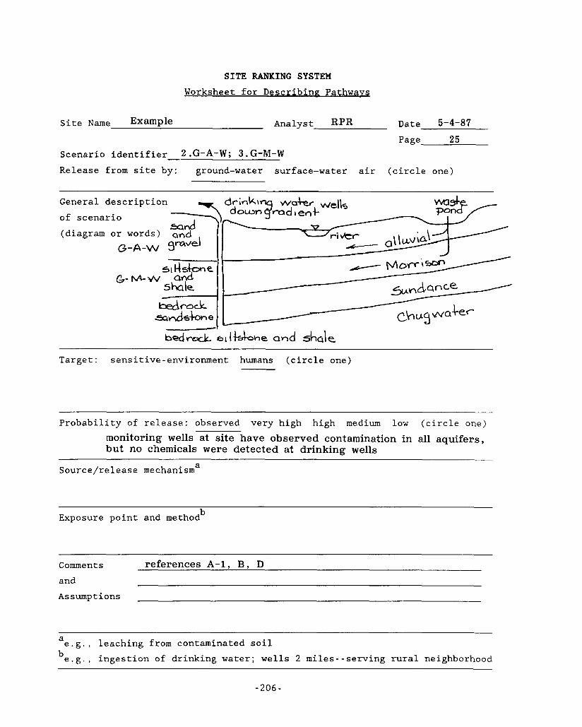
SI’PE RANKING SYSTEM Worksheet for Describing Pathwavs
Page 25 Scenario identifier 2 .G-A-W; 3. G-M-W Release from site by: ground-water surface-water air (circle one)
~~ ~
Target: sensitive-environment humans (circle one)
~~~ ~
Probability of release: observed very high high medium low (circle one) monitoring wells at site have observed contamination in all aquifers, but no chemicals were detected at drinking wells
a Source/release mechanism
b Exposure point and method
Comments references A-1, B , D and As sump t ions
a
b e.g., leaching from contaminated soil e.g., ingestion of drinking water; wells 2 miles--serving rural neighborhood
- 206 -
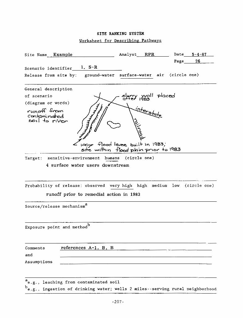
SITE RANKING SYSTEM
Worksheet for DescribinP - Pathways
Site Name Example Analyst RPR Date 5-4-87 Page 26
Scenario identifier 1. S-R Release from site by: ground-water surface-water air (circle one)
General description of scenario (diagram or words)
run& -c- Cw\klWi*k&Zd ~ o r 1 -+o r t V w
Target: sensitive-environment humans (circle one)
4 surface water users downstream
~~~
Probability of release: observed very high high medium low (circle one)
runoff prior to remedial action in 1983
a Source/release mechanism
b Exposure point and method
Comments references A-1, B , B and Assumptions
a b e.g., leaching from contaminated soil e.g., ingestion of drinking water; wells 2 miles--serving rural neighborhood
- 207 -
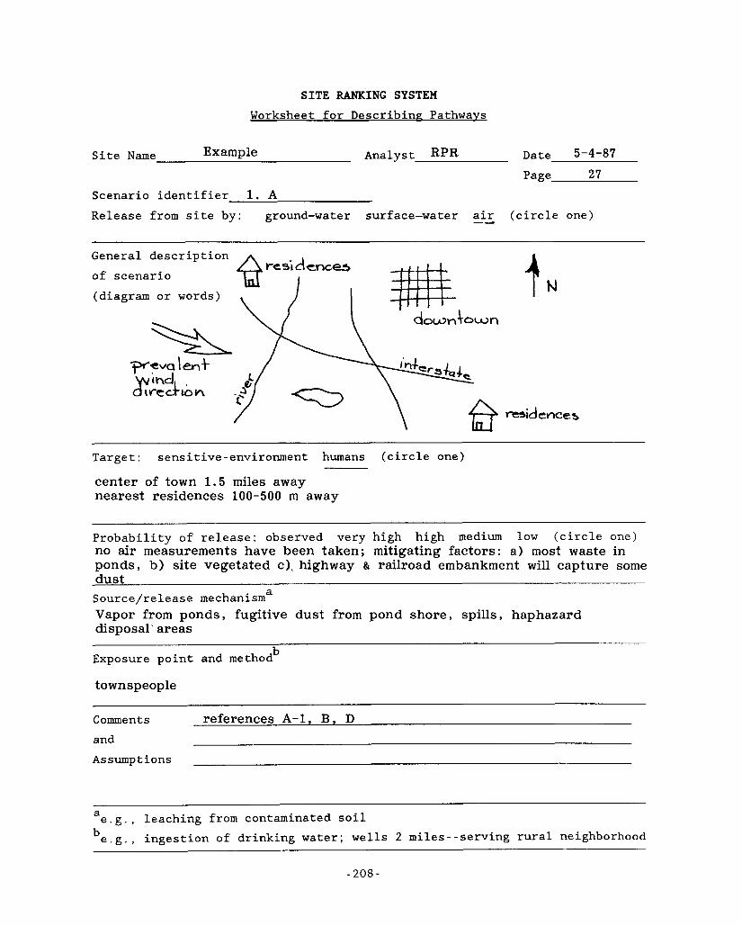
SITE RANKING SYSTEM Worksheet for DescribinP Pathways
Site Name Example Analyst RPR Date 5-4-87
Page 27 Scenario identifier 1. A Release from site by: ground-water surface-water a& (circle one)
General description of scenario (diagram or words)
%
Target: sensitive-environment humans (circle one)
center of town 1 . 5 miles away nearest residences 100-500 m away
Probability of release: observed very high high medium low (circle one) no air measurements have been taken; mitigating factors: a) most waste in ponds, b) site vegetated c), highway & railroad embankment will capture some dust Sour c e/re 1 e as e mechan i sma Vapor from ponds , fugitive dust from pond shore , spills , haphazard disposal I areas
~ ~~
b Exposure point and method
townspeople
Comments references A-1, B y D and Assumptions
a
b e.g., leaching from contaminated soil e.g., ingestion of drinking water; wells 2 miles--serving rural neighborhood
- 2 0 8 -
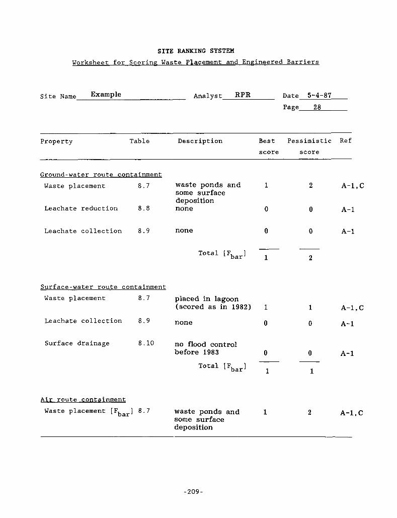
C .
L
SITE RANKING SYSTEM Worksheet for Scoring - Waste Placement and Engineered Barriers
Site Name Analyst RPR Date 5-4-87
Page 28
Property Table Description Best Pessimistic Ref score score
Ground-water route containment
A-1 , C Waste placement 8.7 waste ponds and 1 2 some surface deposition
Leachate reduction 8.8 none 0 0 A-1
Leachate collection 8.9 none 0 0 A-1
Surface-water route containment Waste placement 8.7
Leachate collection 8.9
Surface drainage 8.10
Air route containment
Waste placement [Fbar] 8.7
placed in lagoon (scored as in 1982)
none
no flood control before 1983
waste ponds and some surface deposition
1
0
A-1, C 1
0 A-1
0 0 A-1
1 1
2 A-1 , C 1
- 209 -
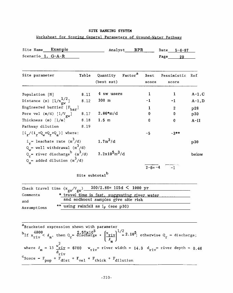
SITE WINKING SYSTEM Worksheet for ScorinP General Parameters of Ground-Water Pathway
Site Name Example Analyst RPR Date 5-4-87
Scenario 1. G-A-R P a g e 2 9
Site parameter Table Quantity Factora Best Pessimistic Ref (best est) score score
Population [N] 8.11 4 s w users
8 . 1 2 300 m Distance (m) [l/x 1/2 3 gw
Engineered barrier [F J Pore vel (m/d) [ 1 / V 3 8.17 2.86*m/d
Thickness (m) [l/m] 8.18 1 . 5 m Pathway dilution 8.19 [ir/(ir+%+Qr+Qa)] where:
3
bar
gw
1 .7m3/d 3 i = leachate rate (m /d) Qw= well withdrawal (m /d)
Qa= added dilution (m /d)
r
5 3 2 . 2 ~ 1 0 m /d Qr= river dischargeb (m 3 /d) 3
1 1 A-1, C
-1 A-1, D -1
1 2 P28 0 0 P30 0 0 A-I1
-5 -3**
P30
below
b Site subtotal
Check travel time (x /V ) 300/2.86= 105d < 1000 yr gw gw
Comments * travel t i m e is f a s t , sumresting river w a t e r and and sediment samples give site risk
A s sump t ions ** using ra in fa l l as i, (see p30)
a Bracketed expression shown with parameter
If Xriv r r b 4800 57 l o 5 1 /2
< Rm, then Q = jisczarge r;:] = 2 - lo5; otherwise Q = discharge;
n L
W where Rm = 15 = 6700 w = river width = 1 4 . 3 driv= river depth = 0.46
Score = F
r iv dr iv
C pop + Fdist + Fvel + Fthick + Fdilution
- 210 -
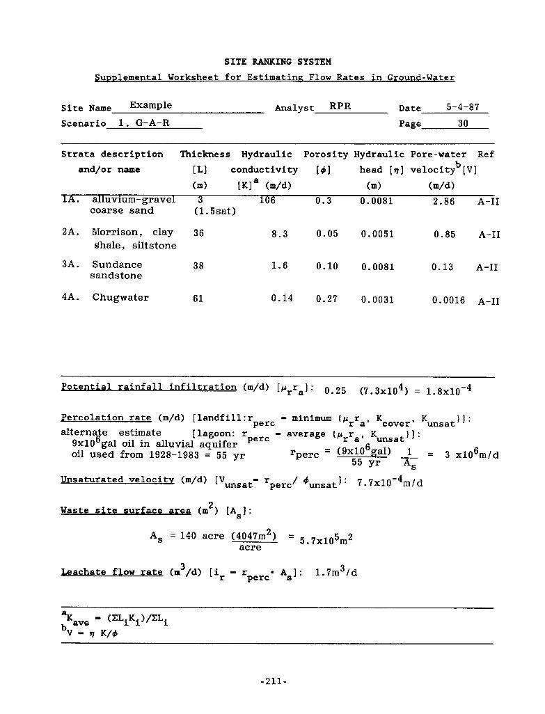
c
._c
h
1
L
I.L
L
-L
I-
-
SITE RANKING SYSTEM
Sumlemental Worksheet for EstimatinF - Flow Rates in Ground-Water
Site Name Analyst RPR Date 5-4-87
Scenario 1. G-A-R Page 30
Strata description Thickness Hydraulic Porosity Hydraulic Pore-water R e f
and/or name [L] conductivity [ 4 ] head [ q ] velocity [VI b
(m) [KIa (m/d) (m) (m/d) ’1A. alluvium-gravel 3 106 0 .3 0.0081 2.86 A-I1
coarse sand ( 1 . 5 s a t )
2A. Morrison, clay 36 shale, siltstone
8 . 3 0.05 0.0051 0.85 A-I1
38 1 . 6 0.10 0.0081 0.13 A-I1 3A. Sundance sandstone
4A. C h u g w a t e r 6 1 0.14 0.27 0.0031 0,0016 A-11
Percolation rate (m/d) [landfill:rperc = minimum ( p r r a’ Kcover* Kunsat , I : alternate estimate [lagoon: rperc - average (prra, Kunsat 11:
9x10 gal oil in alluvial a q u i f e r = ( g x d g a l ) 1 = 3 x l 0 6 m / d oil used f rom 1928-1983 = 55 yr rperc - 55 yr A,
Unsaturated VelocitY (m/d) [Vunsat- rperc/ 4unsat1 : 7 . 7 ~ 1 0 -4 m / d
Waste site surface area (m 2 ) [As]:
A, = 140 acre (4047m2) = 5.7x10 5 2 acre
3 Leachate flow rate (m /d) [ir - rperc* A s ] : 1.7m3/d
-211-
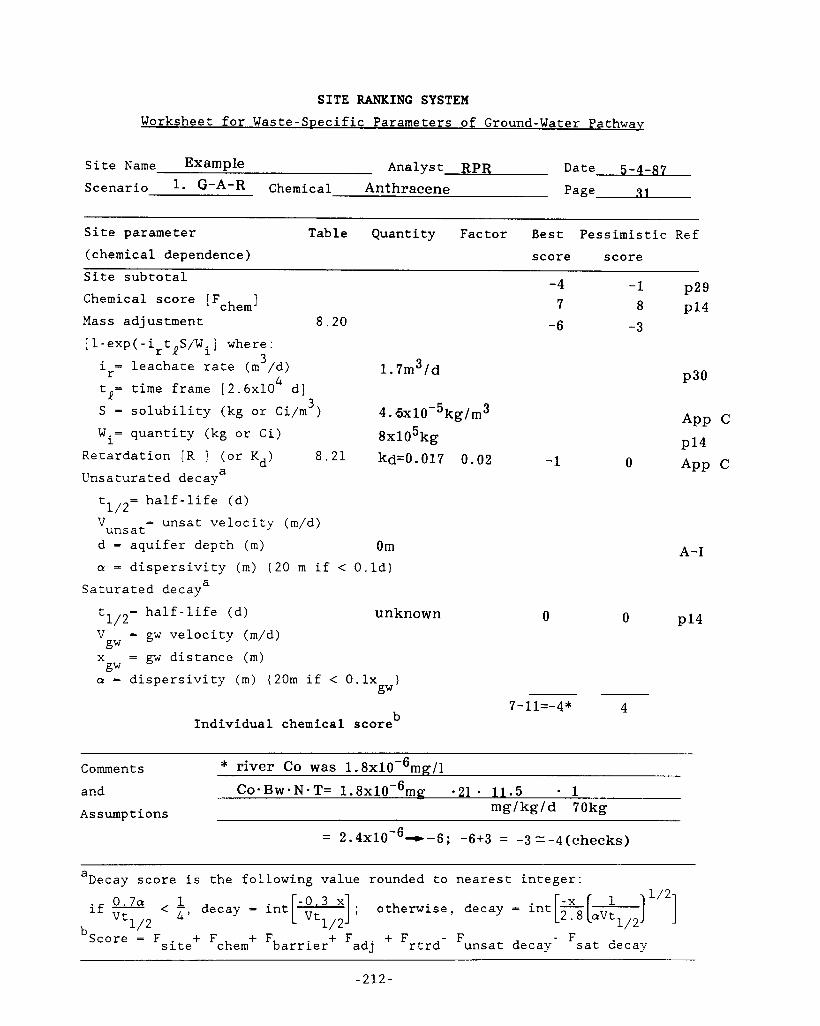
SITE RANKING SYSTEM Worksheet for Waste-Specific Parameters of Ground-Water Pathwav
- - Site Name Example Analyst RPR Date
Scenario 1 . (3-A-R Chemical Anthracene Page.?1
Site parameter Table Quantity Factor Best Pessimistic Ref
(chemical dependence) score score
-1 P29 7 8 P14
-4 Site subtotal Chemical score [Fchem]
Mass adjustment 8.20 -
-6 -3 [l-exp(-i t S/W.] where: r l 1 3
P30
APP c
-1 0 APP c
i = leachate rate ( m /d) t = time frame [2.6x10 d] S = solubility (kg or Ci/m )
W.= quantity (kg or Ci)
1. 7 m 3 / d
4 . 6 x 1 0 - ~ k g / r n ~
Retardation [R ] (or Kd) 8.21 kd=O. 017 0 . 0 2 Unsaturated decaya
4 r R 3
8x10⁵kg P14 1
half-life (d) = unsat velocity (m/d)
5/2= 'uns a t d = aquifer depth ( m ) Om Q - dispersivity ( m ) (20 m if < O.ld)
A-I
a Saturated decay
0 0 P14 5/2= half-life (d) u n k n o w n V = gw velocity (m/d) x = gw distance ( m )
a = dispersivity ( m ) (20m if < 0 . 1 ~ )
b
P iv
gw
Individual chemical score 7-1 1=-4 * 4
Comments * river Co was 1 . 8 ~ 1 0 - ~ m g / l
and Cos Bw - N - T= 1 .8x lO%g -21 * 11 .5 - 1 mg/kg/d 7 0 k g Assumptions
= 2 . 4 ~ 1 0 - ~ - - 6 ; -6+3 = -3 - - 4 ( c h e c k s )
~~~~
Decay score is the following value rounded to nearest integer: a
1 1/2 if 0.7a < - decay - int ; otherwise, decay = int["[-) 2.8 aVt ] 1 / 2 4 '
1/2 Vt
bScore = F~~~~ + Fchem+ Fbarrier+ Fadj + Frtrd- Funsat decay- Fsat decay
- 212 -
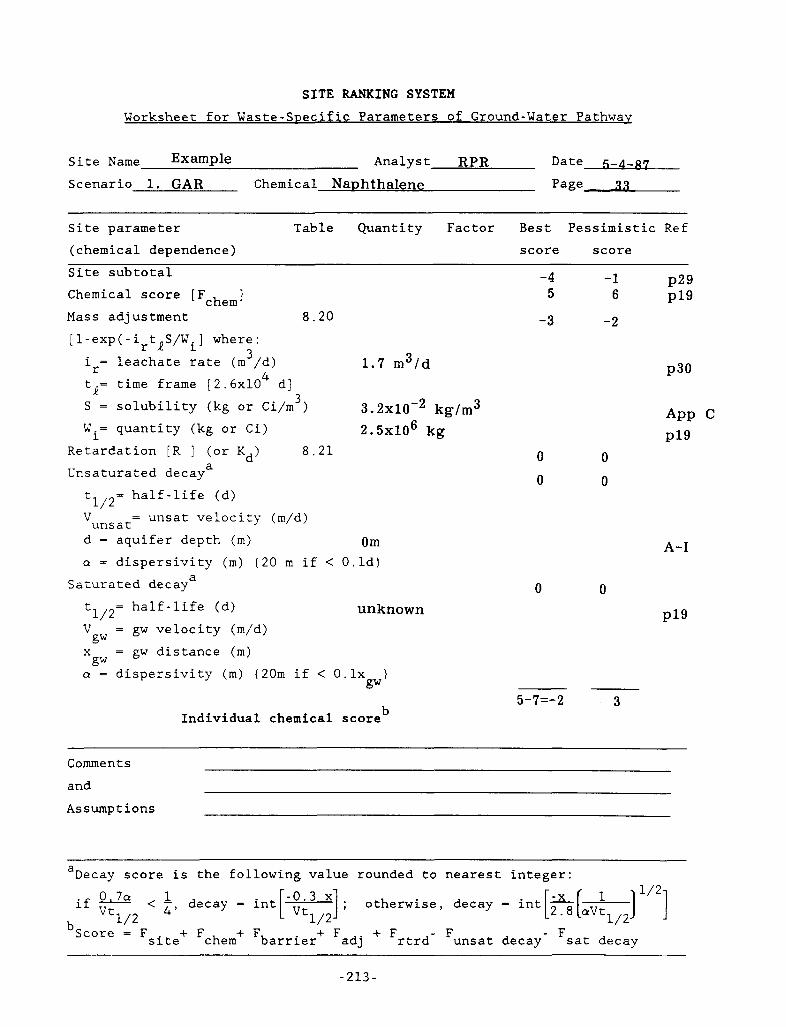
1
.-
SITE RANKING SYSTEM Worksheet for Waste-Specific Parameters of Ground-Water Pathway
Site Name Example Analyst RPR Date 5-4-87
Scenario 1. GAR Chemic a 1 Naphthalene Page--
Site parameter Table Quantity Factor Best Pessimistic Ref (chemical dependence) score score
-4 -1 P29 Chemical score [Fchem] 5 6 P I 9
Site subtotal
8.20 -3 -2 Mass adjustment [l-exp(-irtRS/W.] where:
1 . 7 m 3 / d
3 . 2 ~ 1 0 - ~ k g / m 3
3 1 i = leachate rate (m /d) t = time frame [2.6x10 d] S = solubility (kg or Ci/m )
W.= 1 quantity (kg or Ci) 2 . 5x10⁶ kg
4 r 1 3
Retardation [R ] (or K ) 8.21 Unsaturated decay
d a
t1,2- half-life (d)
'uns at d = aquifer depth (m) Om
= unsat velocity (m/d)
Q = dispersivity (m) (20 m if < O.ld) a Saturated decay
5/2= half-life (d) u n k n o w n V = gw velocity (m/d) x = gw distance (m) Q = dispersivity (m) (20m if < 0 . 1 ~ )
gw gw
gw
b Individual chemical score
0
0
0
0
0
0
5-7=-2 3
P30
A-I
P I 9
and Assumptions
a Decay score is the following value rounded to nearest integer: -
1 1/2 1 ; otherwise, decay - int[2(avt ] ]
1/2 < 4, decay - 0 . 7 a if
1/2 bScore E Fsite+ Fchem+ Fbarrier+ Fadj + Frtrd- Funsat decay- Fsat decay
-213-
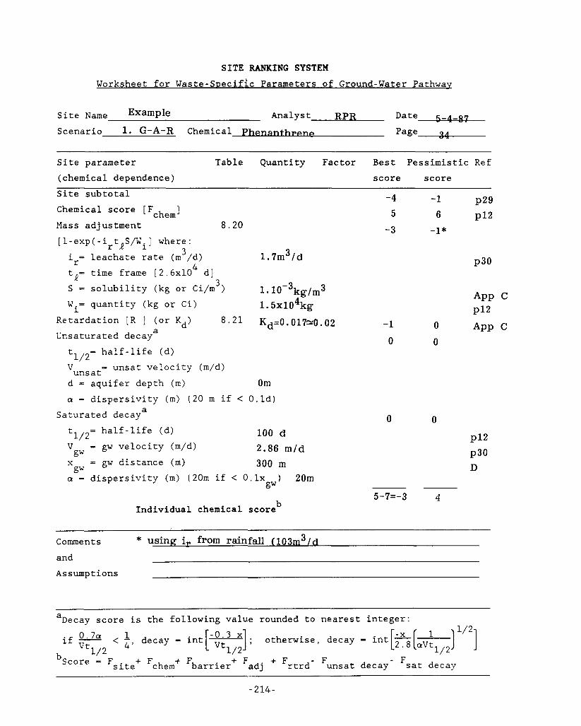
SITE RANKING SYSTEM Worksheet for Waste-Specific Parameters of Ground-Water Pathway
Site Name- Analyst RPR Date
Scenario 1. G-A-R ChemicalPhenanthrPJIP Page 21
Site parameter Table Quantity Factor Best Pessimistic Ref (chemical dependence) score score Site subtotal Chemical score [Fchem] Mass adjustment 8.20 [1-exp(-i t S/Wi] where:
3 r l ir= leachate rate (m /d) t = time frame [2.6x10 d] S = solubility (kg or Ci/m )
W.= quantity (kg or Ci)
4
3 a
1 Retardation [R ] (or Kd) 8.21 Unsaturated decay a
half-life (d) = unsat velocity (m/d)
5/2- 'unsat d = aquifer depth (m)
1. 7 m 3 / d
Om
-4 5
-3
-1
0
-1 P29 6 P I 2
-1*
P 3 0
0 0
a = dispersivity (m) (20 m if < O.ld) a Saturated decay
P I 2 P 3 0
5/2= half-life (d) 100 d V = gw velocity (m/d) 2 . 8 6 m / d x = gw distance (m) 300 m a = dispersivity (m) (20m if < 0 . 1 ~ 1 20m
gw gw D
P -- 5-7=-3 4 b Individual chemical score
comments and Assumptions
* using i, from rainfall (1031-11 3 / ,
a - .^ Decay score is the following value rounded to nearest integer: L/Z
1 / 2 2.8 aVt
1 4 ' < - decay = int ; otherwise, decay = ir~t[&(~) ] if
"Ore = Fsite+ Fchem+ Fbarrier+ Fadj + Frtrd- Funsat decay- Fsat decay b 1/2
-214-
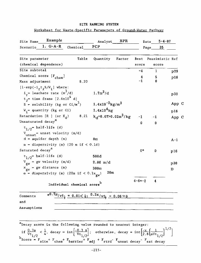
*I-
SITE RANKING SYSTEM
Worksheet for Waste-Specific Parameters of Ground-Water Pathwav
Site Name Analyst RPR Date 5-4-87 Scenario 1. (3-A-R Chemical PcP Page 35
Site parameter ~~ ~
Table Quantity Factor Best Pessimistic Ref (chemical dependence) score score Site subtotal -4 1 P29 Chemical score [F ]
Mass adjustment 8.20 chem 4 5 PI6
-1 0
[1-exp(-irtaS/Wi] where:
1.7m3/d P30
1. 4x1o4kg PI6
3 ir= leachate rate (m /d) t = time frame I2.6~10 d] S = solubility (kg or Ci/m )
W.= quantity (kg or Ci)
4
3 1.4~10-~kg/m~ APP c
8.21 kd=0.07>0.02m3/kg -1 -1 APP c
I
1 Retardation [R ] (or Kd) Unsaturated decay a 0 0
half-life (d) 5/2- = unsat velocity (m/d) 'unsat
d = aquifer depth (m) Om a - dispersivity (m) (20 m if < O.ld)
a Saturated decay
5/2- half-life (d) 500d
V = gw velocity (m/d) 2.86 m / d gw
A-1
O * 0 PI6
P30 300m D x = gw distance (m)
a = dispersivity (m) (20m if < 0 . 1 ~ ) 20m gw
gw
Individual chemical score 4-6=-2 4 b
*0*7cr/vt~ = 0.01<&; 0*3x/vt~ = 0.06'0 z Comments and
Assumptions
Decay score is the following value rounded to nearest integer: a
1/2 1 - O e 3 ; otherwise, decay = in.["[ ] ] if 0.7a < -, decay - int[ Vt 4
"Ore = Fsite+ Fchem+ Fbarrier+ Fadj + Frtrd- Funsat decay- Fsat decay 1/2
2 . 8 aVt ] 1/2 1/2 Vt
b
-215-
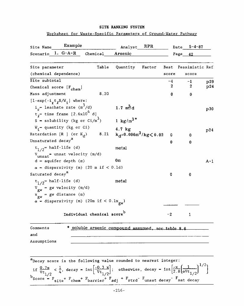
SITE RANKING SYSTEM Worksheet for Waste-SDecific Parameters of Ground-Water Pathway
Site Name Example Analyst RPR Date 5-4-87
Scenario 1. G-A-R Chemical A r s e n i c P a g e 4 2
Site parameter Table Quantity Factor Best Pessimistic Ref (chemical dependence) score score Site subtotal -4 -1 P29 Chemical score [Fchem] 2 2 P24
1 . 7 &/d P30
Mass adjustment 8.20 0 0 [1-exp(-irtnS/Wi] where:
3 i = leachate rate (m /d) t = time frame [ 2 . 6 x 1 0 d] S = solubility (kg or Ci/m )
Wi= quantity (kg or Ci)
4 r 1
1 k g / m 3 * 3
4 . 7 kg P24 Retardation [R 3 (or Kd) 8 . 2 1 kd=O. 006m3/kg< 0 . 0 2 0 0
Unsaturated decaya 0 0 5/2= half-life (d) metal
'uns a t d = aquifer depth (m) Om
a = dispersivity (m) (20 m if < O.ld)
= unsat velocity (m/d)
Saturated decaya
A-1
0 0 half-life (d) metal 5/2=
V = gw velocity (m/d) x = gw distance (m) a = dispersivity (m) (20m if < 0 . 1 ~ )
gw gw
gw
-2 1 b Individual chemical score
Comments * soluble arsenic c o m D o U w t n h l ~ 8 . 6
and Assumptions
Decay score is the following value rounded to nearest integer: a . ,* 1 4' if e < - decay - int ; otherwise, decay - int
1 0 bScore e Fsite+ Fchem+ Fbarrier+ Fadj + Frtrd- Funsat decay- Fsat decay
- 216 -
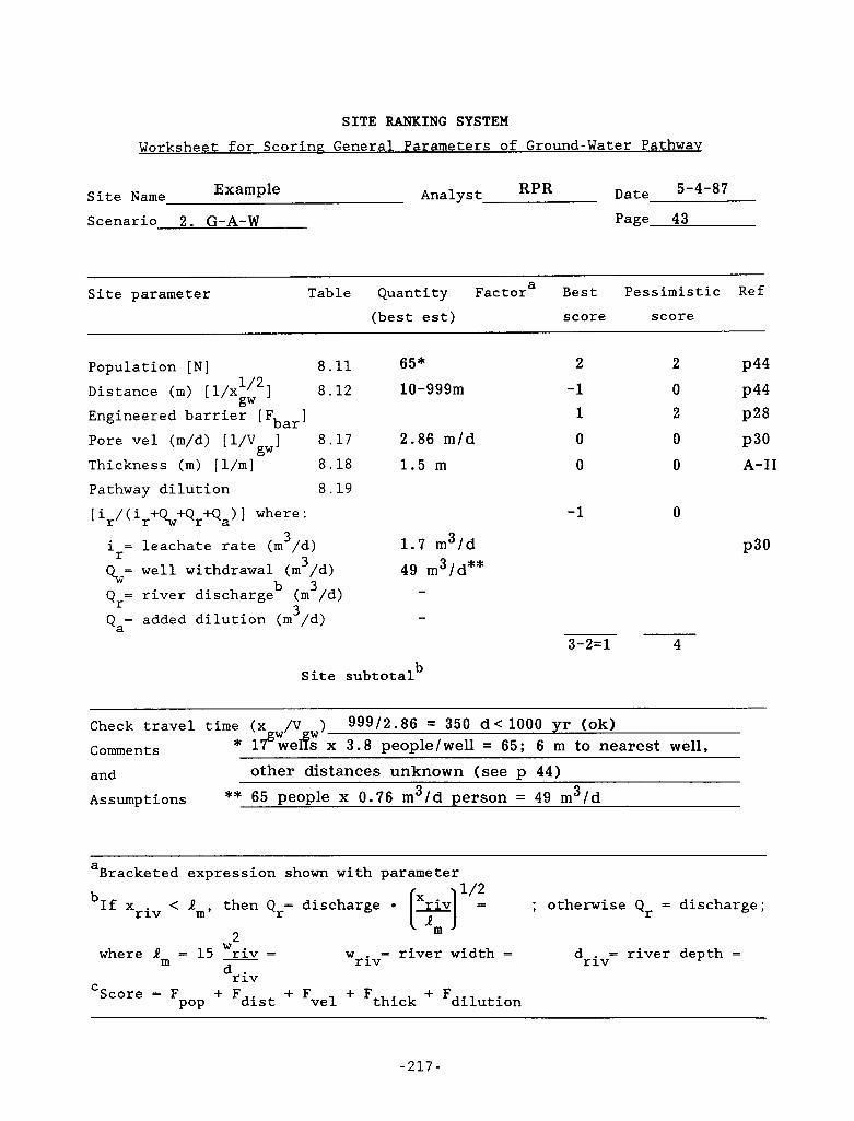
L
zt-
SITE RANKING SYSTEM Worksheet for Scoring General Parameters of Ground-Water Pathway
Example Analyst RPR Date 5-4-87 Site Name Scenario 2. G-A-W Page 43
Site parameter Best Pessimistic Ref a
(best est) score score Table Quantity Factor
Population [ N] 8.11 Distance (m) [l/x 1/2 ] a . 12
gw Engineered barrier [ Fbar] Pore vel (m/d) [1/V 3 8.17 Thickness (m) [l/m] 8.18 Pathway dilution 8.19 [ir/(ir+Qw+Qr+Qa)] where:
gw
3 i = leachate rate (m /d) Qw= well withdrawal (m /d) Qr= river discharge (m3/d) Qa= added dilution (m /d)
3 r
b 3
65* 2
10-999m -1 1
2.86 m / d 0
1.5 m 0
1 . 7 m3/d
49 m3/d** -
b Site subtotal
-1
3-2=1
2 P44
0 P44 2 P28
0 P30 0 A-I1
0
P30
4
Check travel time (x w/v w) Comments and Assumptions
99912.86 = 350 d < 1000 yr (ok) * l?gwelfs x 3.8 p e o p l e / w e l l = 65 ; 6 m to nearest wel l ,
other distances u n k n o w n (see p 44) 3 ** 65 people x 0.76 m 3 / d person = 49 m / d
a Bracketed expression shown with parameter
; otherwise Q = discharge; r 1/2 b < am, then Qr- discharge r;:] - If Xriv
.7 L
W - river depth = dr iv where Rm = 15 riv = w - river width =
Score = F
r iv dr iv
C pop + Fdist + Fvel + Fthick + Fdilution
-217-
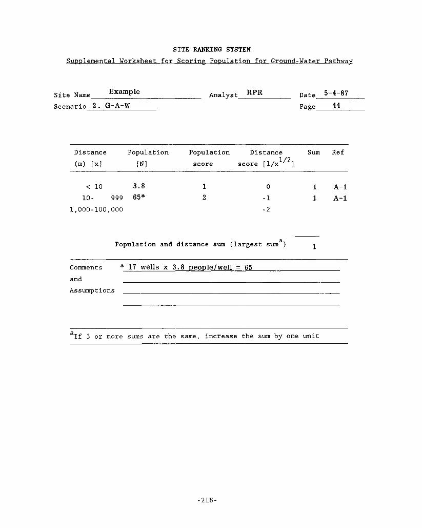
SITE RANKING SYSTEM SuDDlemental Worksheet for Scoring - Population for Ground-Water Pathway
Site Name Example Analyst RPR Date 5-4-87
Scenario 2. G-A-W Page 44
Distance Population Population Distance Sum Ref
(m> [XI [NI score score [l/x 1/2 3
< 10 3 . 8 10 - 999 65*
1,000-100,000
1 2
0
-1 - 2
1 A-1 1 A-1
a 1 Population and distance sum (largest sum )
Comments * 17 wells x 3 . 8 people/well = 65 and Assumptions
a If 3 or more sums are the same, increase the sum by one unit
- 2 1 8 -
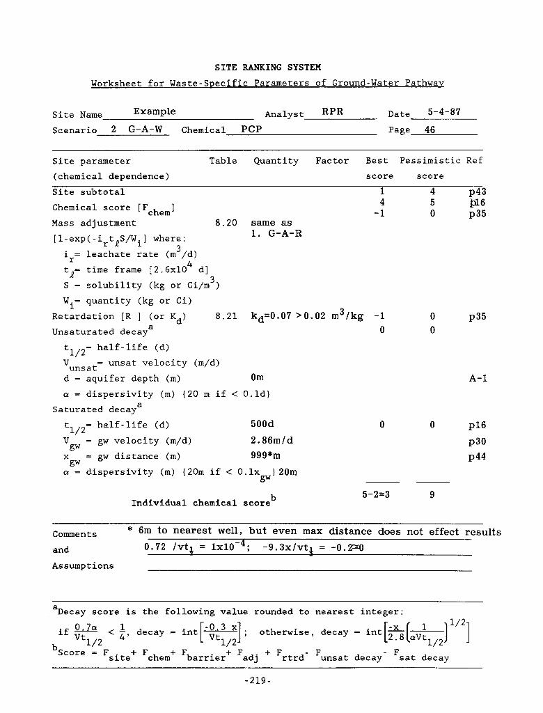
SITE RANKING SYSTEM Worksheet for Waste-SDecific Parameters of Ground-Water Pathway
Site Name Example Analyst RPR Date 5-4-87
Scenario 2 G-A-W Chemical PCP Page 46
Site parameter Table Quantity Factor Best Pessimistic Ref (chemical dependence) score score
Site subtotal 1 4 P43 Chemical score [Fchem] - Mass adjustment 8.20 same as [1-exp(-i t S/Wi] where: 1. G-A-R
r l '1
i = leachate rate (m3/d) t = time frame [2.6x10 d] S = solubility (kg or Ci/m )
4 r B 3
Wi- quantity (kg or Ci) Retardation [ R ] (or Kd) 8.21 kd=0.07 > 0 . 0 2 m3/kg -1 Unsaturated decaya 0
half-life (d) = unsat velocity (m/d)
5/2- 'unsat d = aquifer depth (m) Om Q = dispersivity (m) (20 m if < O.ld)
-
4 5 Ipl6 1 0 P35
0 P35 0
A-1
Saturated decaya
5/2= half-life (d) 500d 0 0 P I 6 V = gw velocity (m/d) 2 . 8 6 m / d P30 x = gw distance (m) 999*m P44 gw gw
Q = dispersivity (m) (20m if < 0 . 1 ~ ) 20m gw
b Individual chemical score 5-2=3 9
* 6m to nearest we l l , but even max distance does not effect results Comments and 0 . 7 2 /vtt = 1 ~ 1 0 - ~ ; -9 .3x /v t4 = -0.r-0
Assumptions
Decay score is the following value rounded to nearest integer: 0.7a if - Vt
a
1/2 ; otherwise, decay - int[%[ ] ] 1
1/2 2.8 aVt < 4, decay =
1/2 bScore - Fsite+ Fchem+ Fbarrier+ Fadj + Frtrd- Funsat decay- Fsat decay
-219-

SITE RANKING SYSTEM
Worksheet for Scoring General Parameters of Ground-Water Pathwav
Site Name Analyst RPR Date 5-4-87
Scenario 3 . G-M-W Page 48
Site parameter Table Quantity Factora Best Pessimistic Ref (best est) score score
Population [N] 8 . 1 1
Distance (m) [ l / x 1/2 ] 8 . 1 2
Engineered barrier [F ]
Pore vel (m/d) [1 /V 3 8 . 1 7
Thickness (m) [l/m] 8.18 Pathway dilution 8.19
gw bar
gw
[ir/(ir+Qw+Qr+Q,)l where:
3 3 i = leachate rate (m /d)
Qw= well withdrawal (m /d) Qr= river discharge (m3/d) Q,= added dilution (m /d)
r
b 3
380 3
1372.5m* -2 1
0 . 8 5 m / d 0
36m -2
-4
1 . 7m3/d**
b Site subtotal
3 P49
-2 P49 2 P28
0 P30
-2 P30
-1
P30
~- 4-6=-2 0
Check travel time (x Comments and Assumptions
/V w) 1 3 7 2 . 5 / 0 . 8 5 = 1 6 0 0 d = 4 v r < 1000 vr (ok) * di'%ange to nearest well
** leachate rate into Morrison possibly much less *** Qw= 380 people * 0 . 7 6 m 3 / d / p e r s o n = 6 0 . 8 m 3 / d
a Bracketed expression shown with parameter
; otherwise Qr = 1/2 b < lm, then Q = discharge [y] = If Xriv r
3
w = river width - driv= river WL where Rm = 15 riv =
Score = F
r iv dr iv
C pop + Fdist + Fvel + Fthick + Fdilution
discharge;
depth =
-220-
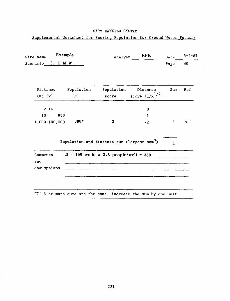
SITE RANKING SYSTEM Supplemental Worksheet for Scoring Population for Ground-Water Pathway
,-
Site Name Example Analyst RPR Date 5-4-87
Scenario 3. G-M-W Page 49
D i s t ance Population Population D i s t ance Sum Ref (m> [XI [ N I score score [l/x 1/2 ]
< 10 10 - 999
1,000-~00,0oo 380* 3
0
-1 - 2 1 A-1
a 1 Population and distance sum (largest sum )
Comments
and Assumptions
N = 100 wells x 3.8 people/well = 380
a If 3 or more sums are the same, increase the sum by one unit
-221-
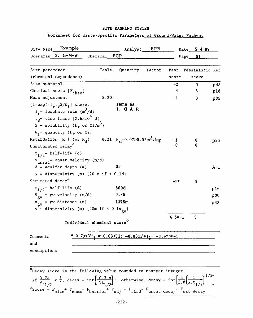
SITE RANKING SYSTEM Worksheet for Waste-SDecific Parameters of Ground-Water Pathway
Site Name Analyst RPR Date 5-4-87 Scenario 3. G-M-W Chemical PCP Page 51
Site parameter Table Quantity Factor Best Pessimistic Ref (chemical dependence) score score Site subtotal -2 0 P48 Chemical score [F chem ] 4 5 PI6
-1 0 P35 Mass adjustment 8.20 [l-exp(-irtRS/Wi] where: same as
i = leachate rate (m 3 /d) t = time frame [2.6x10 d] S = solubility (kg or Ci/m )
1. G-A-R 4 r
R 3
W.= quantity (kg or Ci) 1
Retardation [R ] (or Kd) Unsaturated decay
8.21 kd=0.07>0.02m3/kg a
half-life (d) 5/2= = unsat velocity (m/d) 'unsat
d = aquifer depth (m) Om a = dispersivity (m) (20 m if < O.ld)
a Saturated decay
half-life (d) 500d V = gw velocity (m/d) 0.85 x = gw distance (m) 1375m a = dispersivity (m) (20m if < 0 . 1 ~ )
5/2=
gw gw
gw
b Individual chemical score
-1 0
-1*
0 0
P35
A-1
0
PI6 P30
P48
4-5=-1 5
Comments * 0.7@/Vt~ = 0.03<&; -0.03x/Vt1= -0.97 '-1 1 Y
and Assumptions
a Decay score is the following value rounded to nearest integer: 1/2
< 4, 1 decay = int [;x8 [CYV:~/~~ ] ; otherwise, decay = int ~ - 0 .7a if - Vt 1/2
bScore = F site+ Fchem+ Fbarrier+ Fadj + Frtrd- Funsat decay- Fsat decay
-222-
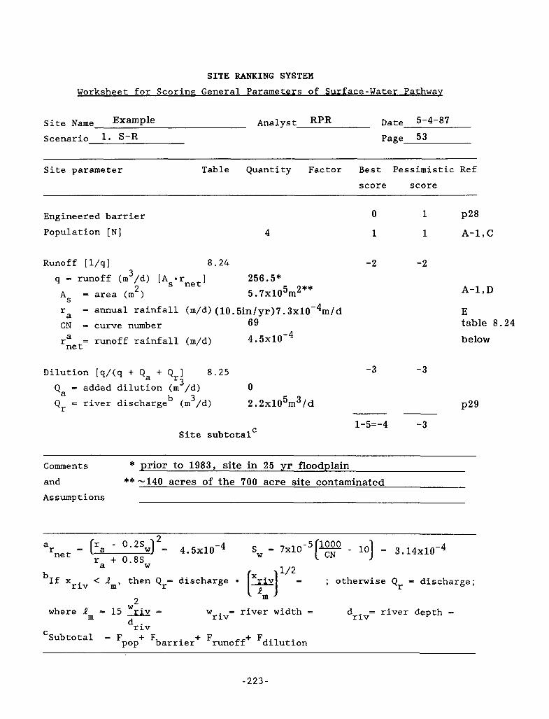
SITE RANKING SYSTEM Worksheet for Scoring General Parameters of Surface-Water Pathway
Site Name Analyst RPR Date 5-4-87
Scenario 1- S-R Page 53
Site parameter Table Quantity Factor Best Pessimistic Ref score score
Engineered barrier Population [N] 4
0 1 P28
1 1 A-1 , C
Runoff [1/q] 8 . 2 4 -2 -2 256.5* 5.7~10 m
3 q = runoff (m /d) As = area (m )
[As-rnet] 5 2** 2
r CN - curve number 69
ra = runoff rainfall (m/d) 4. 5x1OV4
- annual rainfall (m/d) (10.5in/yr)7.3~10-~m/d a
net
A-1 , D
E table 8.24 below
Dilution [q/(q + Qa + Qr] 8 . 2 5 -3 -3
0 2.2~10 m / d
3 Qa = added dilution (m /d) Qr - river dischargeb (m3/d) P29
5 3
1-5=-4 -3 Site subtotal'
Comments * prior to 1983, site in 25 yr floodplain and **-140 acres of the 700 acre site contaminated Assumptions
I - 5 1000 2 p a - 0*2sw] = 4 . 5 ~ 1 0 - ~ a r
b
sW - 7x10 [yy - 10 = 3.14~10-4 r + 0.8Sw net
1/2 a
; otherwise Q - discharge; r If xriv < lm, then Qr- discharge r?] - where lm = 15 riv = w = river width = d - = river depth =
2 W
r iv r 1V dr iv
C = Fpop+ Fbarrier+ Frunoff+ Fdilution
-223-
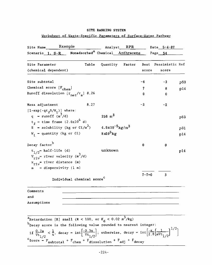
SITE RANKING SYSTEM Worksheet of Waste-Specific Parameters of Surface-Water Pathway
Site Name Example Analyst RPR Date 5-4-87 Scenario 1. S-R Nonadsorbeda Chemical Anthracene Page 54
Site Parameter Table Quantity Factor Best Pessimistic Ref (chemical dependent) score score
Site subtotal Chemical score [Fchem] Runoff dissolution [r /ra] 8.26 net
-4
7 0
-3
8 0
Mass adjustment 8.27 -3 -2 [1-exp(-qtRS/Wi)] where:
256 m3 3 q - runoff (m /d) 4 tR - time frame (2.6~10
S - solubility (kg or Ci/m 3 ) 4 . 5 ~ 1 0 - ~ k g / m ~ d)
Wi - quantity (kg or Ci) 8 do5kg
P53
P14
P53
P31
P14
b Decay factor half-life (d)
t1/2= 3 - river velocity (m /d) 'r iv x - river distance (m) r iv a - dispersivity (1 m)
unknown 0 0
P14
-~ 7 - 7=0 3
Individual chemical scoreC
Comments and Assumptions
~
3 Retardation [R] small (R < 100, or Kd < 0.02 m /kg) a
bDecay score is the following value rounded to nearest integer: .^ if
Score - 7a < ' 4 ' decay = int ; otherwise, decay - int [2.8 -x [aVtl/) '''1
C 1/2 Fsubtotal + Fchem + Fdissolution + Fadj + Fdecay
-224-
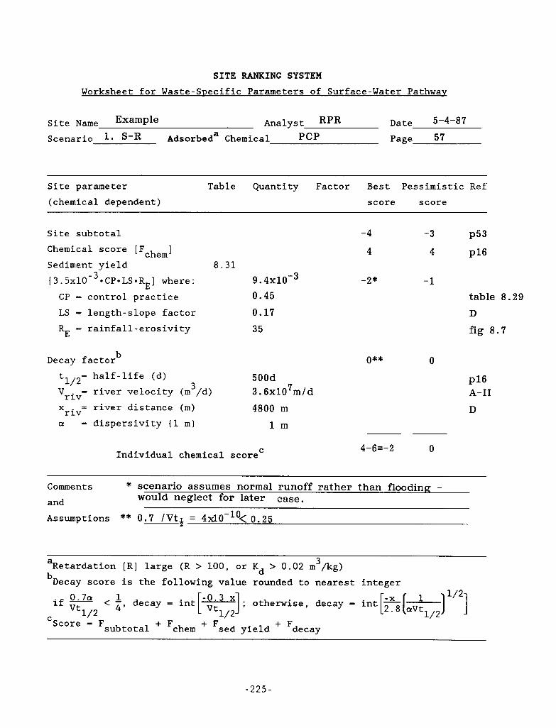
SITE RANKING SYSTEM
Worksheet for Waste-Specific Parameters of Surface-Water Pathway
Site Name Analyst RPR Date 5-4-87
Scenario 1. S-R Adsorbeda Chemical PCP Page 57
Site parameter Table Quantity Factor Best Pessimistic Ref (chemical dependent) score score
Site subtotal Chemical score [F ]
Sediment yield 8.31 [ ~ . ~ x ~ O - ~ * C P * L S * R E 3 where: 9 . 4 ~ 1 0 - ~
chem
CP = control practice 0 . 4 5
LS = length-slope factor 0 . 1 7
RE - rainfall-erosivity 35
b Decay factor
half-life (d) 5 0 0 d 3 . 6 x 1 0 7 m / d 5/2= 3 - river velocity (m /d) 'r iv
x = river distance (m) 4800 m r iv Q = dispersivity (1 m) l m
-4 -3 P 5 3
4 4 P I 6
-2* -1 table 8
D
fig 8 . 7
0** 0
P16 A-I1
D
4-6=-2 0 Individual chemical scorec
Comments and
* scenario assumes normal runoff rather than flooding - would neglect for later case.
Assumptions ** 0 . 7 /vt* = 4 ~ l 0 - ~ ~ < 0 . 2 5
3 Retardation [R] large (R > 100, or Kd > 0.02 m /kg) a
bDecay score is the following value rounded to nearest integer 1/2
if
Score =
< - 1 decay - int[ -0.3 Vt x ] ; otherwise, decay = int[=[ ] ] 1/2 2.8 aVt
1/2 4'
C 1/2 Fsubtotal + Fchem + Fsed yield + Fdecay
-225-
29

SITE RANKING SYSTEM Worksheet for Scoring PoDulation and Distance for Air Pathway
Analyst RPR Date 5-4-87 Site Name Example Scenario l . A P a g e 5 9
Distance Population Population D i s t ance Sum Ref 2 (m> [ X I [NI score score [l/x ]
0- 17 17- 55 56- 175 176- 550 4
551- 1750 729 1751- 5500 1 4 , 7 7 7 5501-17500
0 -2 -4
-5 -6 -7 -8
-4 D , A - 1
-3 D , A - 1 -3 D ,A-1
Largest sum a -3
Waste placement score 1
b Site subtotal -2
Comments and Assumptions
a
bAdd largest sum and waste placement score If 3 or more sums are the same, increase the sum by one unit
- 226 -
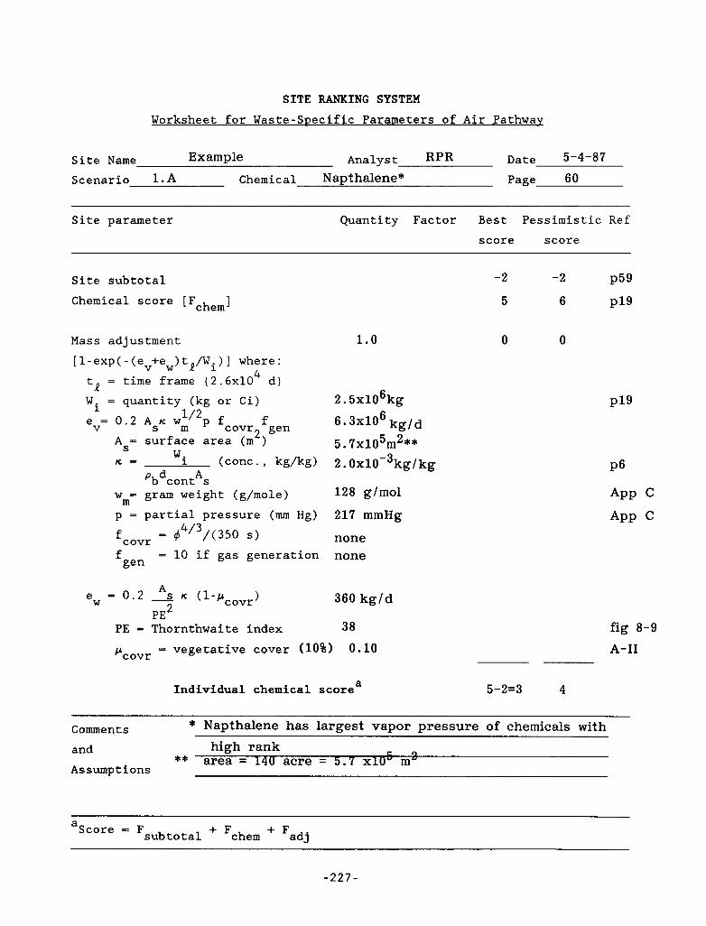
SITE RANKING SYSTEM Worksheet for Waste-Specific Parameters of Air Pathwav
Site Name Example Analyst RPR Date 5-4-87
Scenario 1 . A Chemical Napthalene" Page 60
Site parameter Quantity Factor Best Pessimistic R e f
score score
Site subtotal Chemical score [Fchem]
Mass adjustment 1 . 0 [l-exp(-(ev+ew)tR/Wi)] where:
d) 4 tl = time frame (2.6~10
W. = quantity (kg or Ci) e = 0.2 A IC w
2. 5 x 1 0 6 k g 1/2 f 6 . 3 ~ 1 0 6 kg/d
5. 7x10⁵m2**
1
P fcovr2 gen V s m As= surface area (m )
I C = 'i (cone. kg/kg) 2 . 0 ~ 1 0 - ~ k g / k g
w = gram weight (g/mole) 128 g/mol p = partial pressure (mm Hg) 217 mmHg
none f f = 10 if gas generation none
'bdcontAs m
= 4 4 / 3 / ( 3 5 0 S ) covr
gen
A
PE2 360 kg/d e = 0.2 2 IC (1-p )
W c ovr
PE = Thornthwaite index 38
"covr = vegetative cover (10%) 0.10
Individual chemical scorea
-2 -2 P59
5 6 P I 9
0 0
P I 9
f i g 8-9
A-I1
5-2=3 4
Comments and high rank
Assumptions
* Napthalene has largest vapor pressure of chemicals wi th
c r ) ** area = 140 acre = 5.7 x10" m y
a Fsubto tal + Fchem i- Fadj Score -
- 227 -
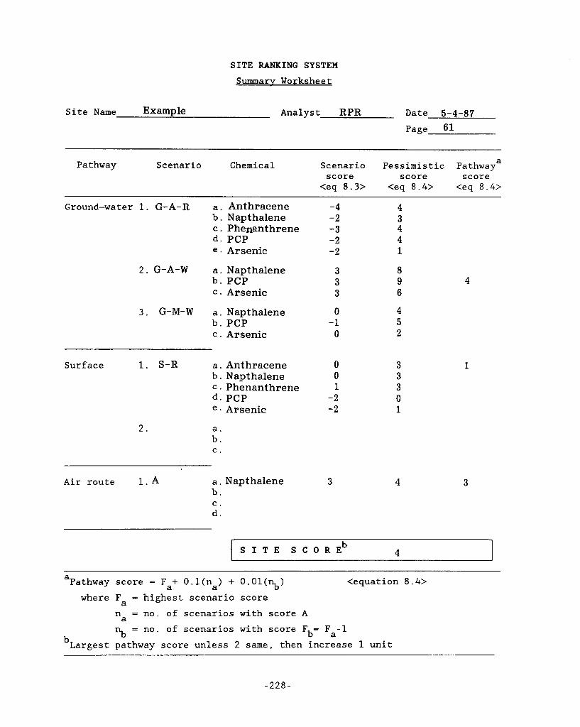
SITE RANKING SYSTEM Summary Worksheet
Site Name Example Analyst RPR Date 5-4-87
Page 61
Pathway Scenario Chemical Scenario Pessimistic Pathwaya score score score
<eq 8 . 3 > <eq 8 . 4 > <eq 8.4>
Ground-water 1. G-A-R a. b .
d. e.
2 . G-A-W a. b.
C.
C.
3 . G-M-W a. b . C.
Anthracene Napthalene Phenanthrene PCP Arsenic
Napthalene PCP Arsenic
Nap t halene PCP Arsenic
Surface 1. S-R a. b.
d. e.
C.
2 . a. b . C .
Anthracene Nap t halene Phenanthrene PCP Arsenic
-4 -2 -3 -2 -2
3 3 3
0 -1
0
0 0 1
-2 -2
4 3 4 4 1
8 9 6
4 5 2
3 3 3 0 1
4
1
Air route 1. A a. b.
Napthalene 3 4 3
C. d.
[ S I T E S C O R E b 4 1 Pathway score = Fa+ O.l(na) + O . O l ( n , , )
where Fa = highest scenario score
a
n = no. of scenarios with score A a
<equation 8.4>
n,, = no. of scenarios with score F Fa-1 b= bLargest pathway score unless 2 same, then increase 1 unit
- 2 2 8 -
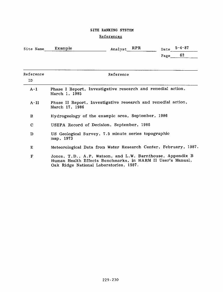
SITE RANKING SYSTEM References
Date 5-4-87 Analyst RPR - Site Name Example
Page 62
Ref e rence Re f e rence ID
A- 1 Phase I Report, Investigative research and remedial action, March 1, 1985
A-I1 Phase I1 Report, Investigative research and remedial action, March 17, 1986
B Hydrogeology of the example area, September, 1986
C USEPA Record of Decision, September, 1986
D US Geological Survey, 7.5 minute series topographic map, 1973
E Meteorological Data from Water Research Center, February, 1987.
F Jones, T.D., A.P. Watson, and L.W. Barnthouse, Appendix B Human Health Effects Benchmarks, in HARM I1 User's Manual, Oak Ridge National Laboratories, 1987.
2 2 9 - 230

12. APPENDIX C
Chemical Properties of Hazardous Waste
Appendix C presents UCR data for radionuclides and reproduces chemical data from the "Superfund Public Health Evaluation Manual" (EPA, 1986b) (also available on PC floppy disk). This data should help the assessor in applying SRS. The most recent version of the EPA manual should be referenced for additions to the chemical waste data. Following are explanations of tables, table headings, and data sources.
Table C.l
Table C.l tabulates UCR data for numerous radionuclides with half-lives greater than 100 days. The calculation of the radionuclide UCR values are described below.
Calculation of radionuclide UCR. Provided that cancer risk per rem [CR] ] or inhalation [DFair] for a and the dose factor for either ingestion [DF
radionuclide are known, calculation of an equivalent UCR is straightforward: oral
UCR = CR DForal,b * z where
CR = cancer risk per rem (cancer risk/rem) = dose factor from ingestion for organ b (rem per pCi/day) DForal
Z = w (70 kg) if quantity of waste [Wo] is expressed in Ci; otherwise,
e (converts mg to pCi times 70 kg) 13 - w n X = 1.3~10 (Xe/mw)
= (70x10 E) ( 6 . 0 2 ~ 1 0 ~ ~ atom/mol) ('e day-') (3.2~10'~ dis/day/Ci) (mw g/mol)
m = gram molecular weight of nuclide (g/mol) n = number of atoms per mass of isotope W
Xe = effective isotope decay or body elimination rate (day -1 )
Normally for radionuclides, the quantity [W 3 is expressed in terms of its activity (Ci) rather than its mass (kg). For this case, Z converts UCR
0
-231-
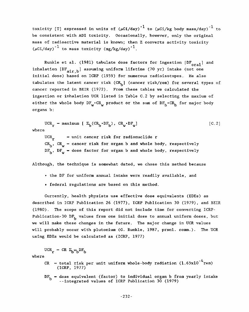
toxicity [TI expressed in units of (pCi/day)-' to (pCi/kg body mass/day)-' to be consistent with AD1 toxicity. Occasionally, however, only the original mass of radioactive material is known; then Z converts activity toxicity (pCi/day) to mass toxicity (mg/kg/day) -I.
Runkle et al. (1981) tabulate dose factors for ingestion [DForal] and inhalation [DFair,b ] assuming uniform lifetime (70 yr) intake (not one initial dose) based on ICRP (1959) for numerous radioisotopes. He also tabulates the latent cancer risk (CR,] (cancer risk/rem) for several types of cancer reported in BEIR (1972). From these tables we calculated the ingestion or inhalation UCR listed in Table C.2 by selecting the maxium of either the whole body DFw*CRw product or the swn of DFb-CR.,, for major body organs b :
UCR, = maximum [ %(C%*DFb), CRw-DFw] [C.21 where
UCR, CR,, CRw - cancer risk for organ b and whole body, respectively DFb, DFw - dose factor for organ b and whole body, respectively
= unit cancer risk for radionuclide r
Although, the technique is somewhat dated, we chose this method because
the DF for uniform annual intake were readily available, and
federal regulations are based on this method.
Currently, health physists use effective dose equivalents (EDEs) as described in ICRP Publication 26 (1977), ICRP Publication 30 (1979), and BEIR (1980). The scope of this report did not include time for converting ICRP- Publication-30 DF values from one initial dose to annual uniform doses, but we will make these changes in the future. The major change in UCR values will probably occur with plutonium (G. Runkle, 1987, prsnl. comm.). The UCR using EDEs would be calculated as (ICRP, 1977)
b
UCRr = CR %wbDFb where
CR = total risk per unit uniform whole-body radiation (1.65~10-~rem) (ICRP, 1977)
DF = dose equivalent (factor) to individual organ b from yearly intake - -integrated values of ICRP Publication 30 (1979)
-232-
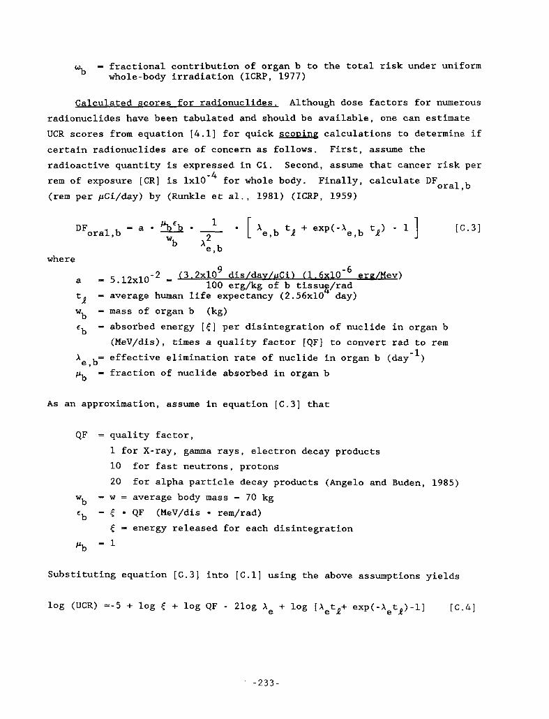
.. L
% = fractional contribution of organ b to the total risk under uniform whole-body irradiation (ICRP, 1977)
Calculated scores for radionuclides. Although dose factors for numerous radionuclides have been tabulated and should be available, one can estimate UCR scores from equation [4.1] for quick scoDine; calculations to determine if certain radionuclides are of concern as follows. First, assume the radioactive quantity is expressed in Ci. Second, assume that cancer risk per rem of exposure [CR] is l ~ l O - ~ for whole body. Finally, calculate DForal,b (rem per pCi/day) by (Runkle et al., 1981) (ICRP, 1959)
where 9 3.2~10 dis/dav/uCi) (1.6~10-~ erdMev)
100 erg/kg of b tissuF/rad a - 5.12x10-~ = 1 - -
tR wb = mass of organ b (kg)
'b
Xe,b= effective elimination rate of nuclide in organ b (day
pb
= average human life expectancy (2.56~10~ day)
= absorbed energy [ E ] per disintegration of nuclide in organ b (MeV/dis), times a quality factor [QF] to convert rad to rem
-1 )
- fraction of nuclide absorbed in organ b As an approximation, assume in equation [C.3] that
QF = quality factor, 1 for X-ray, gamma rays, electron decay products 10 for fast neutrons, protons 20 for alpha particle decay products (Angel0 and Buden, 1985)
wb 'b
= w = average body mass - 70 kg - E QF (MeV/dis rem/rad)
E - energy released for each disintegration pb =
Substituting equation [C.3] into [C.l] using the above assumptions yields
log (UCR) --5 + log E + log QF - 210g Xe + log [XetR+ exp(-XetR)-l] v.41
-233 -
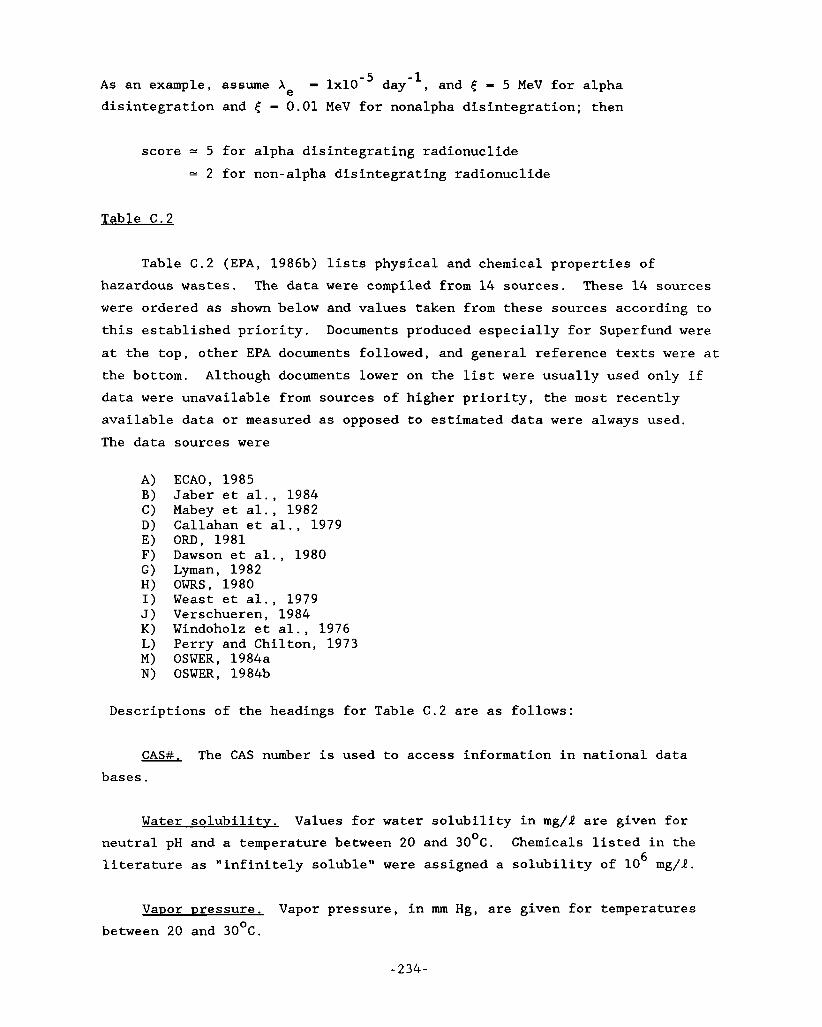
As an example, assume X = l ~ l O - ~ day-', and f - 5 MeV for alpha disintegration and f = 0.01 MeV for nonalpha disintegration; then
e
score = 5 for alpha disintegrating radionuclide = 2 for non-alpha disintegrating radionuclide
Table C.2
Table C.2 (EPA, 1986b) lists physical and chemical properties of hazardous wastes. The data were compiled from 14 sources. These 14 sources were ordered as shown below and values taken from these sources according to this established priority. Documents produced especially for Superfund were at the top, other EPA documents followed, and general reference texts were at the bottom. Although documents lower on the list were usually used only if data were unavailable from sources of higher priority, the most recently available data or measured as opposed to estimated data were always used. The data sources were
ECAO, 1985 Jaber et al., 1984 Mabey et al., 1982 Callahan et al., 1979 ORD, 1981 Dawson et al., 1980 Lyman, 1982 OWRS, 1980 Weast et al., 1979 Verschueren, 1984 Windoholz et al., 1976 Perry and Chilton, 1973 OSWER, 1984a OSWER, 1984b
Descriptions of the headings for Table C.2 are as follows
CAS#. The CAS number is used to access information in national data bases.
Water solubilitv. Values for water solubility in mg/R are given for neutral pH and a temperature between 20 and 3OoC. literature as "infinitely soluble" were assigned a solubility of 10
Chemicals listed in the
mg/R. 6
Vapor pressure. Vapor pressure, in mm Hg, are given for temperatures between 20 and 3OoC.
- 234-
--
I
c
I.
Henry's law constant. Henry's law constant was calculated by
3 vaDor Dressure (atm) molecular weieht (e/mol) water solubility (g/m') H (atm-m /mol) -
Oraanic carbon Dartition coefficient. The organic carbon partition coefficient [KO=] (ml/g) measures the tendency for organics to adsorb onto the organic fraction of soil and is expressed as
mass of solute on solid Dhase/ mass of oraanic carbon P
Koc concentration of solute in solution
Octanol-water Dartition coefficient. The octanol-water partition coefficent [K ] is the equilibrium partition between octanol and water. It indicates the relative affinity of a chemical for non-polar and polar solvents. It is a key variable for estimating other parameters.
ow
Bioconcentration factor. The bioconcentration factor (BCF) measures the tendency for a contaminant in waC,er to accumulate in fish tissue. contaminant concentration in fish tissue is estimated by multiplying surface- water concentration by BCF.
The
Table C.3
Table C.3 tabulates half-lives for hazardous wastes in various media. The half-lives are a combination of various degradation processes (biodegradation, hydrolysis, oxidation, photolysis). The data came either from source A (ECAO, 1985) or source M (OSWER, 1984a).
Table C.4
Table C.4 tabulates EPA toxicity data on noncarcinogenic chemical wastes. with an " @ . "
toxicity score [F ] when evaluating a chemical for SRS.
Those chemicals that also exhibit carcinogenic effects are marked An assessor should use the UCR or AD1 that gives the largest
tox
Subchronic acceDtable intake (AIS). AIS toxicity values are short-term acceptable intake levels.
- 2 3 5 -
Chronic acceDtable intake (AIC). AIC toxic values [designated acceptable daily intake (ADI) in for text] are the long-term acceptable intake levels for a hazardous chemical. As a side note, for EPA, AD1 (also referred to as reference doses [RfD]) designate a subset of AIC values that where developed by the Office of Research and Development in 1985 from compilations other than HEA documents (for example, other agencies or old evaluations).
Table C.5
Carcinopenic Dotencv factors. Carcinogenic potency factors [CPF] are upper 95% confidence limits on the slope of the dose-response curve. reported values are recorded directly from Health Effects Assessment (HEA) or Carcinogen Assessment Group (CAG) documents.
The
Weight of evidence. The weight of evidence column in Table C.5 is classified according to Table C.6, EPA categories for potential carcinogens.
Table C.7
Although Tables C.4 through C.5 provide toxicity information on numerious hazardous wastes, over 65,000 industrial chemicals exist. In addition to the toxicity information of Tables C.4 and C.5, Smith and Barnthouse (1987) (Table C.7) have provided toxicity estimates for many other chemicals. Convert the "benchmark" health effect in Table C.7 to an AD1 by multiplying by ( 10-3mg/pg) (1/70kg) (Alternatively, divide 0.7 by the "benchmark" to obtain UCR) .
Smith and Barnthouse (1987) estimated the benchmark health effect for the chemicals with incomplete toxicity data using the RASH procedure (Jones, et al., 1987). The RASH procedure estimates the toxicity relative to benzo(a)pyrene using data reported in the registry of toxic effects of chemical substances (RTECS) (Tatken and Lewis, 1983).
-236-
References for Appendix C
Angelo, J. A., and D. Buden, 1985. Space Nuclear Power, (Malabar, FL: Orbit Book Company, Inc.), p . 113.
BEIR, 1980. The effects on populations of exposure to low levels of ionizing radiation, Biological Effects of Ionizing Radiations (BE1R)--Advisory Committee, National Academy of Sciences, Washington, DC,
BEIR, 1972. The effects on populations of exposure to low levels of ionizing radiation, Biological Effects of Ionizing Radiations (BE1R)--Advisory Committee, National Academy of Sciences, Washington, DC,
CAG, 1985. Relative carcinogenic potencies among 54 chemicals evaluated by the carcinogen assessment group (CAG) as suspect human carcinogens, U. S . Environmental Protection Agency (EPA), Washington, DC.
Callahan et al., 1979. Water-related environmental fate of 129 priority pollutants, Volumes I and 11, Office of Water Planning and Standards, Office of Water and Waste Management, U.S. Environmental Protection Agency (EPA), Washington, DC. [Source D]
Dawson, et al., 1980. Physical/chemical properties of hazardous waste constituents, U.S. Environmental Protection Agency (EPA), prepared by Southeast Environmental Research Laboratory. [Source F]
ECAO, 1985. Health effects for . . . ( specific chemical), Environmental Criteria and Assessment Office, U.S. Environmental Protection Agency (EPA), Washington, DC. [58 individual documents available for specific chemical or chemical group] [Source A]
ECAO, 1984. Summary data tables for chronic noncarcinogenic effects, Environmental Criteria and Assessment Office, U.S. Environmental Protection Agency (EPA), Washington, DC.
EPA, 1986b. Superfund public health evaluation manual, OSWER Directive 9285.4-1, Office of Solid Waste and Emergency Response (OSWER), U.S. Environmental Protection Agency (EPA), prepared by ICF Incorporated, Washington, DC.
ICRP, 1979. Limits for intake of radionuclides by workers, ICRP Publication 30, Part 1, Annals of ICRP 2 No. 3/4, Supplement to Part 1, Annals of ICRP 3, No. 1-4 (New York: Pergamon Press).
ICRP, 1977. Recommendations of the International commission on Radiological Protection, ICRP Publication 26 (New York: Pergamon Press).
ICRP, 1959. Report of committee I1 on permissible dose for internal radiation, International Commission on Radiological Protection (ICRP), (New York: Pergamon Press).
Jaber, et al., 1984. Data acquisition for environmental transport and fate screening, 600/6-84-009, Office of Health and Environmental Assessment, U.S. Environmental Protection Agency (EPA), Washington, DC. [Source B]
-237-
Jones, T. D. P. J. Walsh, A. P. Watson, L. W. Barnthouse, and D. A. Sanders, 1987. Chemical scoring by a rapid Screening hazard (RASH) method, J. Risk Analysis (in press).
Lyman, 1982. Adsorption coefficient for soils and sediments, Chapter 4 in Handbook of Chemical Property Estimation Methods, Lyman et al., ed., (New York: McGraw-Hill). [Source GI
Mabey, et al., 1982. Aquatic fate process data for organic priority pollutants, Monitoring and Data Support Division, Office of Water Regulations and Standards, Washington, DC, prepared by SRI International [Source C]
OHEA, 1983. Technical support document and summary table for the ranking of hazardous chemicals based on carcinogenicity, External Review Draft, Office of Health Effects Assessment, U . S . Environmental Protection Agency (EPA), Washington, DC.
ORD, 1981. Treatability Manual, Volume I, EPA 600/2-82-001a, Office of Research and Development, U.S. Environmental Protection Agency (EPA), Washington, DC. [Source E]
OSWER, 1984a. Exposure profiles for RCRA risk-cost analysis model, Office of Solid Waste and Emergency Response, U.S. Environmental Protection Agency (EPA), prepared by ENVIRON Corporation, Washington, DC. [Source MI
OSWER, 1984b. Characterization of Constituents from Selected Waste Streams Listed in 40 CFR Section 261, Office of Solid Waste and Emergency Response, U . S . Environmental Protection Agency (EPA), prepared by ENVIRON Corporation, Washington, DC. [Source N]
OWRS, 1980. Ambient water quality criteria documents for ...( spectfic chemical), U.S. Environmental Protection Agency (EPA), Washington, DC [Source HI
Perry, R., and C. Chilton, 1973. Chemical Engineers Handbook, 5th ed. (New York: McGraw-Hill). [Source L]
Runkle, G. E., R. M. Cranwell, and J. D. Johnson, 1981. Risk methodology for geologic disposal of radioactive waste: NUREG/CR-2166, SAND80-1372, Sandia National Laboratories, Albuquerque, NM.
Dosimetry and health effects,
Tatken, R. L., and R. J. Lewis, 1983. Registry of Toxic Effects of Chemical Substances, 1981-1982 ed., National Institute for Occupational Safety and Health, U.S. Department of Health and Human Services, Centers for Disease Control, Cincinnati, OH.
Verschueren, K., 1984. Handbook of Envi onmental Data on Organic Chemicals, 2nd ed., (New York: Van Norstrand/Rei&old Press). [Source J]
Weast, R. C., ed., 1979. CRC Handbook of Chemistry and Physics, (Cleveland, OH: The Chemical Rubber Co.). [Source I]
Windholz, et al., 1976. The Merck Index. [Source K]
- 238 -
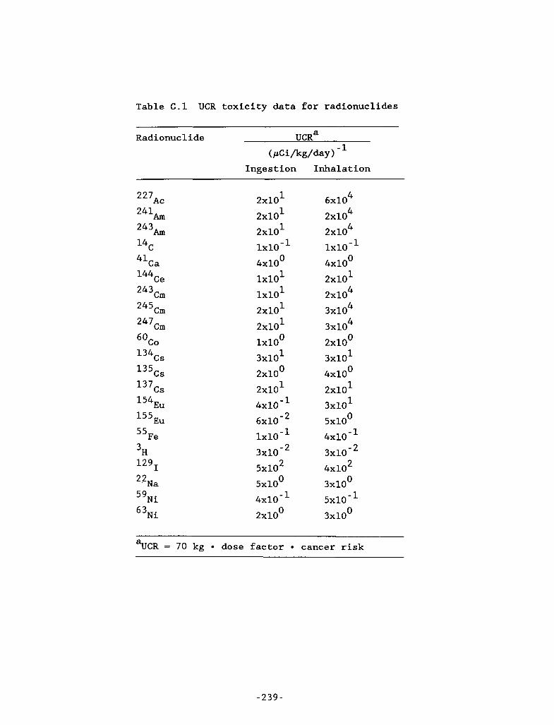
c-
Table C.l UCR toxicity data for radionuclides
Radionuclide UCRa
(pCi/kg/day) Ingestion Inhalation
1 2x10 2X1O1 2X1O1 1x1o-I
l X l O 1
lXlO1 2X1O1 2X1O1 lXlO0
2x1O0 2X1O1
0 4x10
3x10'
4xlO-I 6 ~ 1 0 - ~ 1x10 - 3 ~ 1 0 - ~
2 5x10 0 5x10
4xlO-I 2x10 0
4 4
6x10 2x10 2x1~4
2X1O1
1x10 - 4x10'
4 2x10 3x1O4 3x1o4
3x10' 4x10'
3x10' 0 5x10
4xlO-I 3 ~ 1 0 - ~
2 4x10 3x10' 5xlO-I 3x10'
2x1O0
2X1O1
%CR = 70 kg dose factor cancer risk
- 239 -
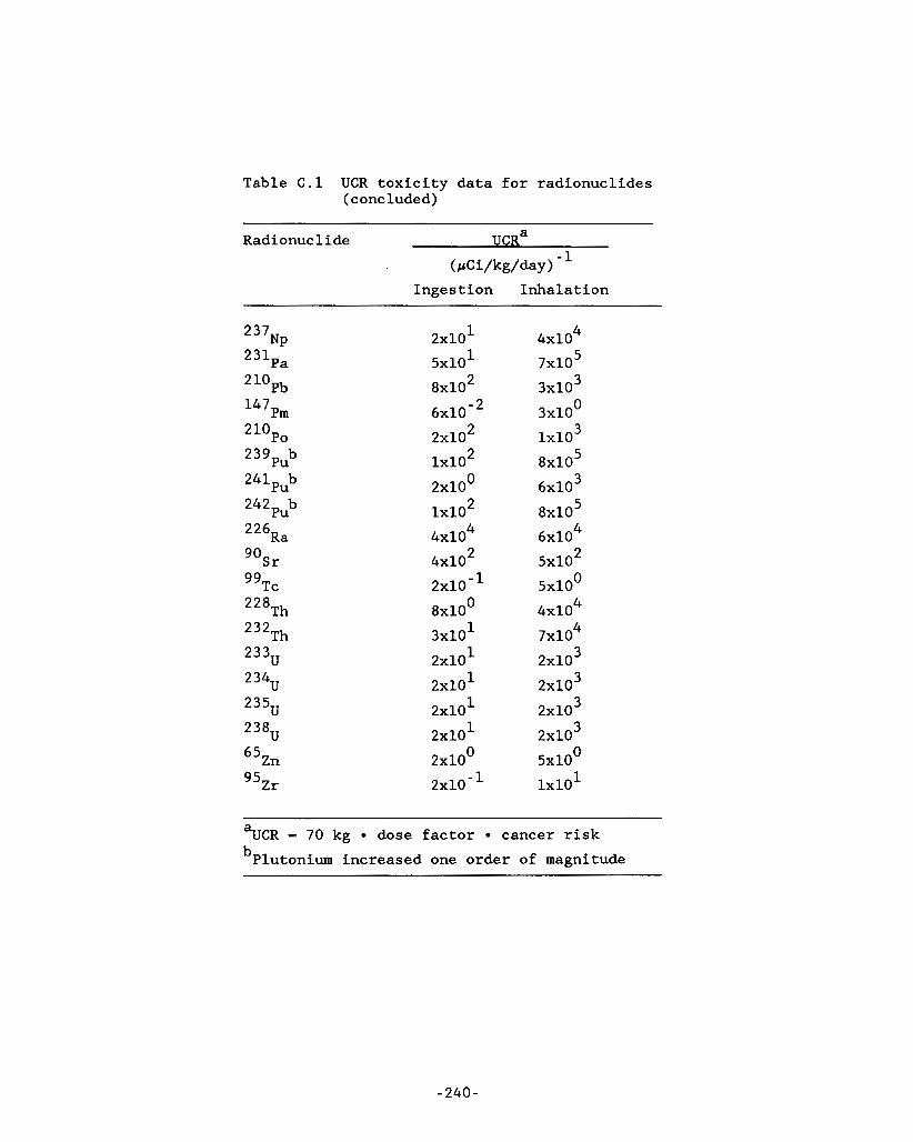
Table C.l UCR toxicity data for radionuclides (concluded)
Radionuclide UCRa (&i/kg/day)
Ingestion Inhalation
NP 237
231~a
2X1O1 5x10' 8x10² 6x10- 2X1O2 1x10² 2x1O0 1x10² 4x10⁴ 4x10² 2x10 - 8x10' 3x10' 2X1O1 2X1O1 2X1O1 2X1O1 2x1O0 2x10 -
4 4x10 7x10⁵ 3x10³ 3x10'
3 1x10 8x10⁵ 6x10³ 8x10⁵
4 6x10 2 5x10
5x10' 4 4x10 4 7x10
2x1~3 2x1~3 2x1~3 2x1~3
lXlO1
0 5x10
%CR - 70 kg dose factor cancer risk bPlutonium increased one order of magnitude
- 240 -
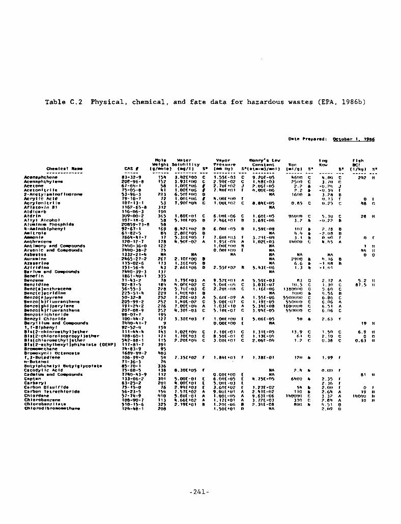
.*."
--
I
Table C . 2 Physical, chemical, and fate data for hazardous wastes (EPA, 1986b)
Chealcml M m r s
Aconmphthena Acenaplrthy lene Ace tone A c e t o n l t r l l e ?-Ace t y I o r lnor Ittornne Acry l lc Acld A c r y l o t r l t r l l a A r l m t o x t n BI Ald l ca rb A l d r l n A l l y l A lco l io l A l r a l nrlr Plmsphlde b - h l nob I plrony I AmltrOle &tila Anthracene A n t l w n y a d Compounds Arsenlc m n d Coqounds Asbestos Auramlno Azmsar Ine Az t r Id I no Bmrlrm mnd Compounds Bener ln Benzene Benz I d Ine Benz( )anthrmcene Benz( c )mer I d Ine Benzo( a )pyrene Banzo( b ) r luorantlrene Benzo( t i 1 )pery lene Benzo( i! )r Iunranthena Benzol r Iclr t o r Ide Benzyl Chlor lda Bery l 1 Iin and Cowounds 1, I -B lphenyl B I s ( 2-ch l o roe t hy I ) e the r BIs(Z-chloro1soprop I )e the r B I s( ch l o rome t hy I )et [e r B I s(2-ethy I Iwxy I tphthm I a te ( DCHl Browlc . t hone 8 r o r o x y n l l OCtmnomte I.3-Butmdlene n-Butnno 1 Birty I phtha I y I Bu cy I g 1 yco I te Cmcodyllc Acld Cmdmlw and Compounds captmn Cm rba r y I Cmrbon O l s u l f l d e Carbon let r i c h l o r Ida Chlordane Chlorobenzene Chlorobenzl l a t e h I orod I b r o a a chon.
83-32-9 2OC-9G-8 61-64-1 75-05-8 53-9G-3 79-10-7 107- 13- I 1167-65-8 116-06-3 3V9-00-2 107- 11)-G 20859-71-8 92-67- 1 61-82-5 76Gh- h I - 7 120- I? - 7 74hO-3G-0 7400-38-2 1332-21-b 2065-27-2 115-02-6 15 1 - 56-11 7OhO-39- 3 1861-W-1 71-L3-2 ?2-87-5 JG-55-3 225-51-h 50-32-8 205-99-2 191-211-2 207-08-9 98-07- 7 loo- 1111 - 7 7ll'lO-l~l-7 92-52-18 1 11-011-b 108-60-1 502-88-1
' ) 117-81-7 7h-83-9 1689 - 99 - 2 106-99-0 71-36-3 85-70- 1 75-60-5 71110-83-9 133-06-2 63-25-2 75-15-0 56-23-5 57-7L-9 108 - 90 - 7 510- 15-6 120-118-1
15h 152 58 11 1
2:! I 72 53
312
365 58 58
1 G9 84 I 7
I 7 8 122 75 MA
26 7 I 7 3 h3
1 3 7 335
78 1811 278 229 252 752 276 252 195 127
9 15lr I h 3 I 7 1 115 39 1 95
h03 5h 7h
336 138 I12 301 2v 1
76 15h 5 I O 113 325 208
I 90 I.8OC-01 c 5.1nc*o5 u 8.h?14(12 o 2.80L+05 6
11.5fJC-07 A 5 .111~405 r
MA 2 .10~400 B 1.36C405 B 2.661406 0
1.75C+Ol A
5.7VC-03 C
I.2OC-Vl A 1.hUC-07 C 7.OOL-011 A *.10t-01 c 3.30C*03 r
h . o n t + o ~ c 1.~iu1401 B
1 . 0 2 ~ 4 0 ~ 1 c P.POC*OII c I . 7 O C + 0 3 C
7.35L402 F
8 .3OC405 r
5.M)C-01 C I ( . W C * O l t ?.9QC+OJ L 7.57t*02 A 5.601-01 A L.66C402 A 2.19t*01 e
6.OnC-06 C 2.hGC+Ol 0
6.00t -05 o
1.95c-nl1 A I . noc 400 w 0 . nnr *(IO c
7.Gllt+IJl f
MA
9.57C4ltl A 5.0f1t-I14 C z.zvc-on c
5.6OC-09 A 5.OOL-lJ7 C I.0lC-10 A 5.1nt-or c
i . o n c 4 0 0 c o.oot+no t
8.5oc-ni c 7.10t -01 C
1.001*0 l c
I . O * C * 0 1 r
o.ouc400 t 6.OOC-05 L 5.0Ilt - 0 3 t 3.GWL*VZ t 9.OUL+Ol A 1 .OOC-(I5 A 1.17t401 A 1.30C-V6 B I .50t401 D
MA
8.04C-115 MA
1 . Got -115 3.69C-I16
I . 59t -00
i.n~t-ni MA
3 . ? l t - f l r l
MA MA MA MA MA
5.b3C-06 MA
5.59C-03 3 . 0 3 C - l J 7 1. lGt-06
MA 1.55C-UG 1.i9c-fJ5 5 . 3hC-08 3.9hL-05
5.06t -05 MA
I . 3 i t 4 5 1.1 3t-011 2.06t-014
( . T a t - O l
MA MA
h . 7 5 ~ - 0 5
1.~3r-02 2 . 4 I t - 0 2 9.63E -06 3.77L-03 7.3lIC-08
MA
l16110 75110
2 . 7 7 . 2
ihim
0 . 0 5
96VO0 1 . 7
I f 1 7 11 , (I I . I
oiimo
NA 79110
6.G 1 . 1
ni I O . 5
1 IOO~INJ 1l1l10
550Vlll l l l 550lltlfJ
l6OlJllfl0 5511000
50
11.9 (I1
1 . 2
170
7.11
6WJO
511 1 I O
15OVfJIl 33n non
C C c b k
C
C k
b e h c
c b k
G C G c C C C C
k
C C C
L
k
b
c c C (: k
5.3u c -11.77 0
7 . ( 8 0 -7.110 0 n.on r 4.115 A
MA
-1.118 B - 1 . 1 1 1
11. I G 0
7 . 1 2 A 1 . 3 0 c 5.60 C 0.56 0 6.06 C
6 . 5 1 A 6.116 C
G.OG A
2 .61 r
1.50 c 7.10 c fJ.18 C
t .99 r
n.uo r
2 . 1 5 2 . 1 6 r r 2. vii r 2.64 A 3 .17 A 7.811 A h . 5 1 0 7.119 1)
0 48
28
0
1 h 11 0
5 . 2 8 1 . 5
19
6 . 9 0
0 . 6 1
81
0 19
14000 I O
II
1 r.
II
r
II II 0
11 II
II
II n II
11
r II II II
- 241-
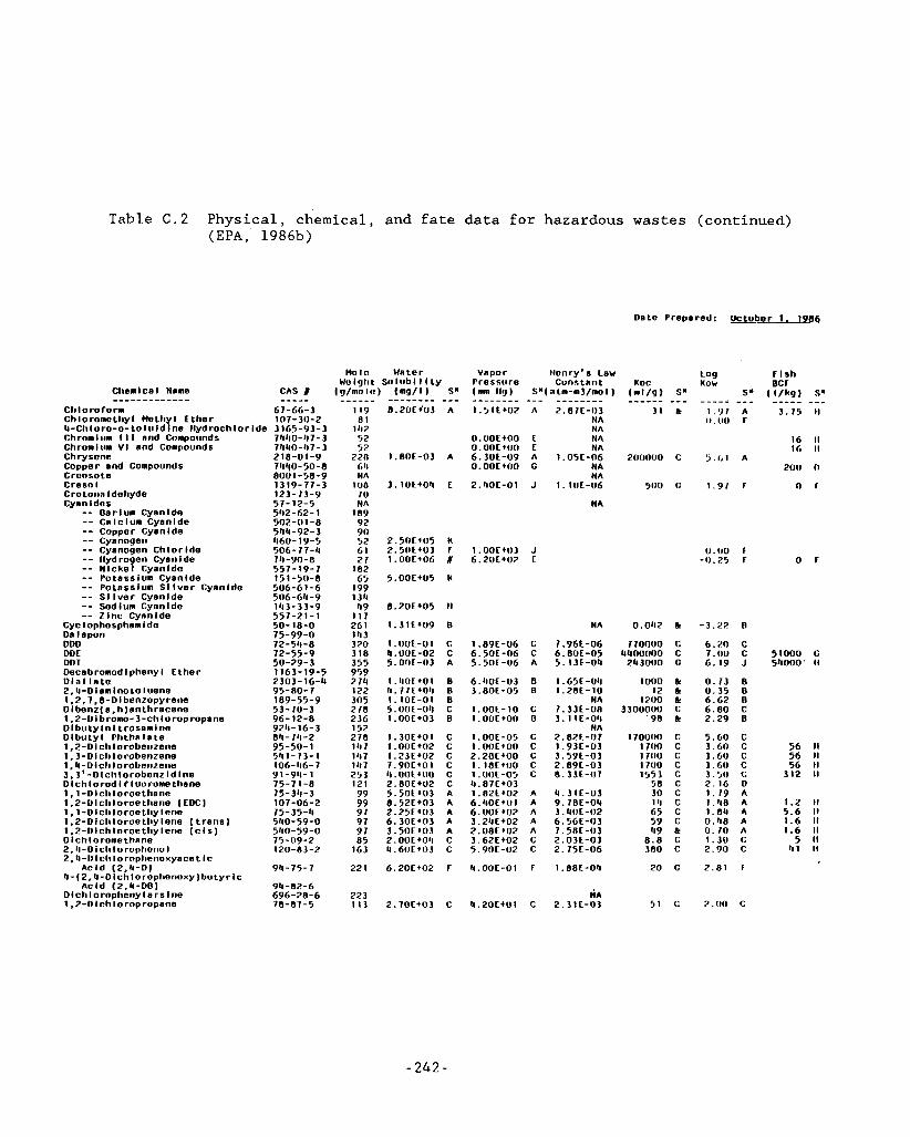
Table C . 2 Physical, chemical, and fate data for hazardous wastes (continued) (EPA, 1986b)
Date Prepared: U l m r 1. 1966
I lcnry 's Law Constsnt
Sn( n t m - a I / m o l )
A 2.81E-113 NA HA
E NA E NA
c N A NA
J 1.10L-06
MA
- - - - -____-_
A i . o 5 ~ - n 6
Cliealcal N s n o CAS I -__---------- ----- ChloroCorm 67-66-3 Ch I orome thy I Me thy I Ether 107- 311-2 4-Chloro-o-to l u l d Ine l l ydroch lo r Ida 1165-93-3 Chroali ia I I I snd Conpocinds 711hO-4 7- 3
Copper and Compounds 74qU-50-8
Crotona ldehyde 123-13-9
Chronlcia V I and Compounds 74hO-h7- 3 Chrysene 2 18-0 1-9
Creosote 8001-58-9 Cresol 13 19- 77- 3
Cyan I de 6 51-12-5
0.00~400 0 . ooc 400
0 . DOE 400 6.30E-09
16 II 16 II
200000 C 5 . 1 ~ 1 A 200 n
O F 500 G 1.91 F 2. # I O € - 0 1
Oa r I ua Cynn I dn Cs lc lua Cyanlde Coppor Cyanlde Cysnogen Cyanogen Ch lor lde llydrogen Cyanide N lcke l Cyanlde Po tabs I urn Cyan Ide Poiosslum SI l v e r Cysnlde S I l v e r CYsnlde
542-62-1 189 502-o 1-8 92 554-92-3 90 460-19-5 52 2.50E405 K 506-17-4 61 2.50E+03 r I.OOE+III J 7 4 -YO - 0 27 I.OOE406 I 6.2oE+02 E 557-19-7 I 8 2 151-50-8 G5 4.00€+05 K 506-61-6 199 506-611-9 1311
0.00 F -0.25 r O F
Sodium Cyanlde Z lnc Cyanlde
Cyc Iophosphsmlde On lapon ODD
DOT Decabronod Ipheny l Ether D l a l l a t e 2,4-Dlamlnoto luene 1.2.7.8-Dlbenzopyrene DI benz( a, h)snthrscene 1.2-0 I b rono- 3-ch I o rop ropane D I bu ty In I t rosaa I ne D l b u t y l Ph ths ls te 1,2-Dichlorobenzene 1,J-Dichlorobenzene 1.4-0 I c l i I o robwnzene 3 . 3 ' -Diclc lorobenz I d Ine Dlch lo rod I f Iuorome thane 1, I -Dlchloroethane 1.2-D I ch I oroe thane ( EDC ) 1.1-0 I ch I oroe thy I ene 1.2-Dlcli lo roe thy I ene ( t r a n i ) 1.2-Dlchloroethylene ( c i s ) D I c l i 1 o rome tha ne 2.4-0 I chlorophcno I 2.4-01 ch loropherroxyace t IC
Acld ( 2 , l l - 0 ) 4-(2,4-Dlchlorophenoxy)butyrlc
Acld (2.1l-DB) Dlchlorophenylarslne 1.2-Dlchloropropane
Dot
. ~ . 143-33-9 551-21 -1 50-18-0 75-99-0 72- 54 - 8 72-55-9 50-29-3 1163- 19-5 2303-16-4 95-R0-7 169-55-9 53-70-3 96-12-0 924-16-3 84- 14-2 95-50-1 54 1 - 7 3- 1 106-46-7 91-94-1 75-71-8 7 5- 34 - 3 107-06-2 15-35-4 540-59-0 540-59-0 7 5 -09 - 2 120-83-2
94-75-7
69 117 26 1 14 3 370 318 355 959 2 7 4
t).20E*05 I1
1.31E409 A
1.00t-01 c 4.0UE-02 C 5.00~-03 A
1.40~401 o i . i o c - o i o 1 . 7 7 E ~ O 4 U
5.00E-04 C I.OOE+Ol 0
NA
7.96E-06 6. 8UE-05 5. IS€-04
1.65E-UII I . 28E- I 0
MA 7 . 3 3 E - 0 8 3 . 1 1 E - 0 4
MA
O . O h 2 t -3.22 A
1.89E-06 C 6.50E-06 C 5.50E-06 A
6.IIOE-03 0 3.80E-05 0
1.0OE-10 c 1.00~400 o
1.00E-05 c .1 .00~400 c 2.20~400 c 1 . 1 8 E 4 0 0 c 1.00E-05 c 4.87E403
6 . 4 O E 4 O 1 A 6.UUE402 A 3.24C~02 A 2.08E402 A 3.62E402 C 5.90E-02 C
4 . O O E - 0 1 F
1.82~402 A
m m o c 440vuno c 243ouo G
1000 k 12 k
12110 t 3300000 C
98 a:
6.70 C 7.00 c 51000 c 6. 19 J 54000' II
0 . 1 3 B 0.35 0 6.62 A 6.80 C 2.29 B
122 305 278 236 152 278 141 14 7 14 7 25 3 121 99 99 91 97 97 05
163
1 . 3 0 E + 0 1 c 1 .00~402 c
z.e.zE-Di 1.93E-03
170wno c 1 7 0 0 c
5.60 C 3.61) C 56 II 3.60 C 56 II 3.60 C 56 II 3.50 C 312 II
3 . 5 9 ~ - ~ 3 2.89E-03 8.33E-07
17110 C 17110 c 1553 C
58 C 3 0 C 14 c
>9 c 49 t 8.8 c 3R0 C
20 G
$5 c
2.ROE402 C 2.16 D 1.19 A 1.48 A
0 .48 A
1.30 C 2.90 C
2.81 F
i . o c A
o . i n A
4.3 I E - 0 3 9.78E-04 3.4lJE-O2 6.56E-I13 7.58E-03 2 . 0 3 E - 0 3 2.75E-06
I . 88E-04
1.2 II 5.6 II 1.6 II 1.6 II 5 II
41 II
6 .30E+03 A 3.50E403 A
4.60E403 C
6.20EW2 F
2.00~40i1 c
2.70€+03 c
22 1
223 1 1 3
94-02-6 696-28-6 78-87-5
NA 2.31E-03 4.2OEtOI C 51 C 2.1tn c
- 242 -
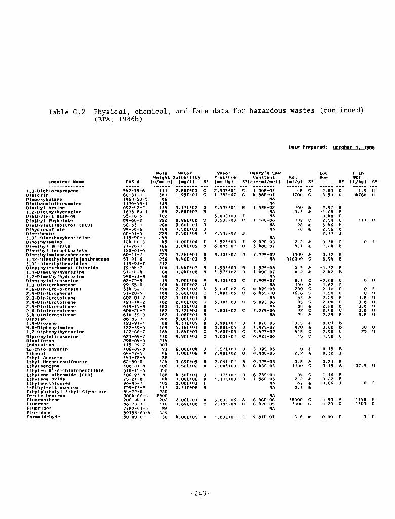
c
Table C . 2 Physical, chemical, and f a t e data fo r hazardous wastes (continued) (EPA, 1986b)
Chenlcnl Mnno ------------- 1.3-01 ch I oropropene D l e l d r l n Dlepovybutano D le thnno ln l t rosnn lne D i e t h y l Ars ine 1.2-1) I e thy1 hydrnz lne D le thy In I t rossnl ne D i e t h y l Fhthnlate D le t l i y 1 s t I I best r o 1 ( DES) Dl l iydrosnf r o l e 0 I me thon tn 3.3' -Dlnethoxybenr l d l n e Dlm?t l iy lanlne Dimethyl S i i l r n te D I no thy I I e repl i thn 1 n t e Dlme thy1 nn I nonznbenzene 7 12-Dlmethylbenz n)nnthrscene 3: 3' -0lne t h I benzld I ne D Ine thy1 cn rznnoy l Ch lo r ide 1,141 Inc thy1 hydraz Ine 1 ,2-0 I IIIO thy I hydraz I ne Dlmethy ln l t rosnnlne 1.3-Dlnltrobenzene 4.6-Dln l t ro-a-cresol 2.4-01 n I t ropheno I 2.3-Dln l t ro to luene 2.4-Dlnl t ro to luene 2.5-01 n I t r o t o I iierie 2.6-Dlnl t ro to luene 3.11-D In I t r o t o I uene DI noseh 1,~l-Dloxnne N, M-Dl phony I m i n e 1,2-Dfpheny I hydrsz I ne Dip ropy I n I t rossnl ne D l s u l r o t o n Endosul fnn Ep lch loro l iydr I n Ethnnol E thy l Acetate E thy I Me tl innesu I tons Le € thy I benzene E thy l - h , 4 ' -d lchlorobenz I l s t e Ethylene Olbromlde ( C O O ) Ethylene Oxlde E t h y 1ene t h I ouren 1 - E t hy I -n I t rosourea Ethy I ph t l in I y I E thy I Clyco I s t e F e r r i c Orxt rnn F 1 uornrithene F luorene r l u o r I des F I iir I done formaldehyde
Mole Water Welglit SoIubI 1 I t y
CAS A (g /no lo ) ( m g / l ) S.
542-75-6 60-57-1 14611-53-5
-1 116-511-7 692 - 4 2 - 7 1615-80- I 55- 18-5 84-66-2 56-53- I 94-58-6 60-51-5 119-90-fl 124 -110- 3 77-78-1 120-61-6 60- 11-7 57-97-6 119-93-7 79-44- 7 57- 19 - 4 540-73-8 62-75-9 99-65-0 5 3 0 - 52 - 1 51-70-5 602-01-7 121-14-2 619-15-0 606-20-2 610-39-9 813-05- 7 123-91-1 122-39-4 122-66-7 621-611-7 298-04-4 115-29-7 106-89-8 611- 17-5 14 1 - 78-6 62-50-0 1 0 0 4 1 - 4 510- 15-6 106-93 -11 75-2 1-0 96-115-1 759- 7 3 -9 811-77-0 9004-66-4 206-411-0 86-73- 7 7 782-4 1-11 59756-60-4 50-00-0
111 38 1 06
1311 134 08
102 222 268 1611 279 ?h11
11 5 126 1'14 225 256 212 108 60 60 74
168 198 180 182 182 182 I82 182 2110
80 169 184 130 274 1107
93 4 6 80
174 106 352 108
114 1 02 117 200
7500 202 l t 6
NA 379
30
2.80E+03 1.95E-01
'I. 17E+02 2.88E+O7
8.96E+fl2 9.60E -03 1 . 5OE+O3 2 . 5 0 ~ +UII
1 .OWE406 3.2llE+05
1.36t+OI 4 .4OE-03
1 . 4 ~ l E ~ 0 7 1.24t+08
l.OOC+06 4.70t+02 2.90E402 5.60L+03 3. l O E + O 3 2 . 4 O E + 0 2 1 . 3 2 E 4 0 3 I . 3Zt+U3 1 .08E+03 5.OWL+Ol 4.3 1E+05 5.76E+01
6.OOE4Oh 1.00€+06
I . 67E+05 1.52E+02
4 . 3 0 E + 0 3 1 .OOE4l)6 2.00E+03 3 . 3 1 E+O8
2 .06E-Ol 1.69EL00
4.00€+05
C C
0 n
C 0 D J
r 0
0 0
0 B
A J C C 0 C B 0 0 J 0 0 C C
J A
0 A
J 0
0 r
A C
K
- 243 -
Vapor l lenry 's Law Prcssrire cons I n n t (mm 119) S~(s tn -m3 /no l )
3.5OF+01
5 .00~400 3.5OE-03
2.50E-02
1.5X403 6.80E -0 1
3.30C-nl
8 . 1 0 ~ 4 0 0
5 . O O E - 0 2 I . 49E-05
5.10E-03
1 . 8OE-02
3.97E401 3. ROC-05 2.6OE-05 4 . ooc- 0 1
1 . 5 7 E + 0 1 7 . ~ I O t + 0 2
2.06C - 0 1 7 . O O E 4 0 0
1.17E401 1 . 3 1 E 4 0 3
5.00E-06 7. io r -o j i
1.00t+01
C C
0
r C
J
r 1)
0
0 D
C
C C
C
C
0 0 C C
0 C
B A
0 0
A C
L
- - - - - - - - 1. 3VE-03 4.58E-07
NA MA
1.48t-02 NA NA
1 . I4E-06 MA NA
NA 9.02E-05 3.48E-07
7.19E-09 MA
1.9ZE-08 1.00E-07
NA 7.90E-07
NA 4.49E-05 6. h5E- 10
N A 5.09E-06
NA 3.21E-06
NA
1.07L-05 1.47E-07 3. WE-09 6.92E-06
3.19E-05 4.98E-05
9.12E-08 6 .43E-03
6. 73E-Oll
NA MA
NA 6.56E-06 6. b2E-05
MA
9.8lE-07
7 . 5 6 ~ - 0 5
Unte Frepsred: ggtober 1. 19-84
160 k 2.77 0 . 3 k -1.60
1112 C 2.5 IJ 78 k 5.116 70 k 7.56
7 . I 1
7 . 7 k -0 .18 1 1 . I k -1.711
o.118
11lOll k 1.12 476000 C 6.94
0 .5 k -1.37 0.7 k -2.112
0.1 C -0.68 15W k 1.67 2110 C 2. 1 0
16.6 C 1.51) 53 k 2.79 115 c 2.00 011 k 2.78 92 C 2 . 0 0 911 k 2.?9
3.5 k 0.01 h70 & 3.60 418 C 2.90
15 C 1.50
10 k 0.15 7.7 k -0.32
3 . 8 & 0 . 2 1 1 I l ) W c 3 . I 5
1111 C 1 . 76 7 .2 b -0.72 67 k -0.6G
0 .1 k
38000 C h.70 7 3 0 0 C 11.70
3 . 6 b 0. OW
0 0 F C I17 G 13 0 J
r 0 1 0
n n
n C 0 I1 r C O E C 0 1) 0 3 . 8 11 C 3 . 8 II 0 3.8 II C 3 .8 II 0 3 . 8 II
0 0 30 C C 25 I1 C
0
n J
0 A 37.5 II
0
J O F n
A 1150 II C 1300 C
F o r
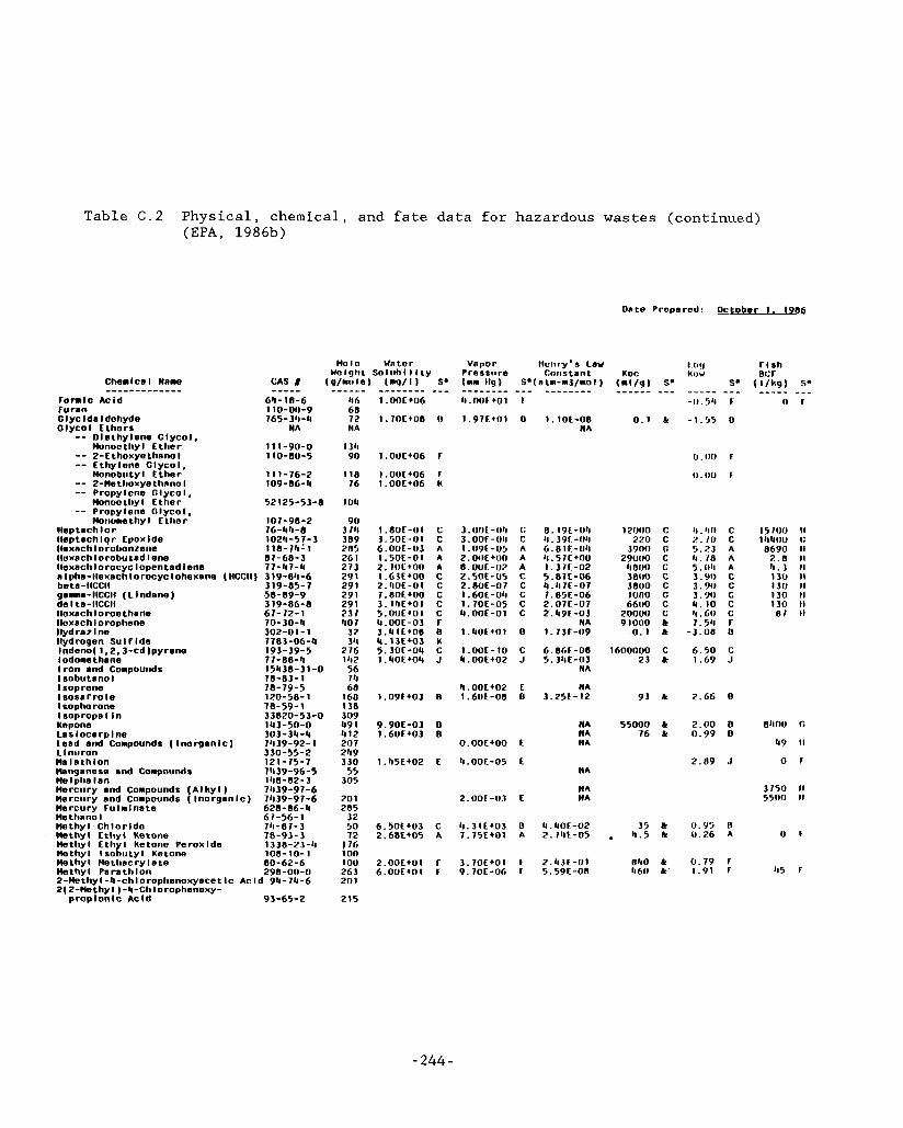
Table C.2 Physical, chemical, and fate data for hazardous wastes (continued) (EPA, 1986b)
Onte Propared: w # o b e r 1. 198-6
Cliemlca I Wnme ------------- Formic Acid Fu ran G I yc Ida I dohyde Glycol Ethors -- Dlethy lene Glycol,
Wnoet l iy l Ether -- 2-Ethoxyethsnol -- Ethylene Glycol, Monobu t y I Ether -- 2-Methoxyetlinnol -- Propylene Glycol , Wnoot l iy l Ethor -- Propylene Glycol. Monoma thy1 E t l i o r
I leptachlor Ileptach lo r Epox Ide Ilexnch lorvbonzene lloxachlorobutad lene llexschlorocycIopentadiene n I pha-Ilexnchlorocyc lohexane
gama-IICCII (Llndsne) de l ts-IICCII llexach loroe thane llexach lorophene tlyd raz I ne Hydrogen S u l f Ida Indene( 1.2.3-cd)pyrene lodomethane I r o n and C O ~ O O U ~ ~ P I sobu t a no I 1 sop rene I sosarro l e I sophorona I sopropa I in Repone La6 I oca r p I ne Lead and Compounds ( Ino rgan lc ) L in t i ron na I a th I on Manganese and Compounds He lplia I a n Mercury and Compounds ( A l k y l J Mercury and Compounds ( Inorganlc) Mercury F u l m I ne t e ne t l imo I MothvI Chlor lde
beta -IlCCII
MethGl Et l ty I Ketone Methyl E thy l Ketone Peroxlde Methyl I sobu ty l Ketone Me thy1 Me thacrv I s r e
Hvlo Wnter Woiglit S o l u h l I I t y
CAS I (g/moto) ( m g / l ) S* ----- ------ _ _ _ _ _ _ _ _ -_- 611-18-6 116 1.00€+06 110-01)-9 68 765-311-18 72 1.70E408 I3
WA NA
11 1-90-0 1311 110-00-5 90 1.OUE406 F
111-76-2 118 l.OUE406 F 109-86- 4 76 1.00E406 I(
52125-53-8 104
107-98-2 90
1024-5?-3 389 1.50E-l) l C 118-711-1 285 6.00E-03 A 87-68-3 261 1.50E-01 A
(HCCII) 319-84-6 291 1.63E400 C 319-85-7 291 2.hOE-01 C 58-89-9 291 7.80E400 C 319-86-8 291 3.10E+01 C 67-72-1 237 5 . O U E 4 O I C
76-411-8 3/11 i . a o ~ - ~ i c
7 7- 11 7 -4 273 2.10~400 A
70-10-4 302-01 -1 7783-06-4 193-39-5 77-88-18 15538-31-0 78-83-1 78-79-5 120-58- 1 78-59- 1 33120-53-0 143-50-0 303-34-4 71139-92-1 310-55-2 121-75-7 7539-96-5 1118-82-1 71139-97-6 7439-97-6 628-86-4
1107 i 1 . 0 0 ~ - 0 3 F 3 2 3.4lE408 B 3 4 4.13E+03 K
276 5.3OE-04 C 1112 1.40E404 J 56 74 68
160 1.09€+03 B 138 309 491 9.90E-03 0 412 1.60€+03 B 207 249 3 3 0 1.55€+02 E 55
305
20 1 285
3.OOE-Oh 3.OOF-011 1.09E-05 2. O l l c ~ o n 8.UUE-02 2.50t-05 2.80E-07 I .60L-04 1.70E-05 9.002-01
C 8 . 1 9 E - U ~ I c h. 391. -011 A 6.8IE-UIl A 11.57r+no A i : j i C - o z C 5.87C-06 c 4 . l l l E - 0 1 C 1.85E-06 C 2.07E-07 C 2.49E-03
NA I . S O E + O l 0 1.73E-09
1.00E-10 C 6.86E-08 4 . 0 0 E 4 0 2 J 5 . 3 4 E - 0 3
NA
~ 1 . 0 0 ~ 4 0 2 E NA 1.60E-08 0 3.25E-12
NA MA
0.00~400 E HA
4.00E-05 E WA
NA 2.00E-03 E HA
woc ( - l /g ) ------
0.1
1201JO 220
3900 29UlIO tl800 3800 3800 luna 6600 20000
0 . I l O F
0.00 F
c (I. 1 1 0 c c 2 . 1 0 c G 5.23 A c S . 10 A C 5 . 0 4 A c 3 . 9 0 c c 3.90 c G 5 : i o c c 4. I O c C 11.60 C
91000 & 7.511 F 0.1 & -3 .08 0
1600000 C 6.50 C 23 k 1.69 J
93 k 2.66 8
15700 II l l l ~ l f l 0 0 8690 II 3.8 II 4 . 3 II 130 II 130 II 130 II 130 II 87 II
55000 & 2.00 0 81100 C
49 II 76 & 0.99 B
2.89 J o r
3750 II 5500 I 1
67-56-1 32 711 - 8 7 - 3 78-93-3 72 2.68E405 A 7.75E401 A 2.752-05 , 4 .5 & 0.26 A O F 1338-23-4 176
50 6.50E403 C 4 . 3 1 E 4 0 3 B 4.4OE-02 35 .4 0.Y5 B
108-10-1 ion 80-62-6 100 2.OOE40I F 3.70E401 E 2.43E-01 8110 & 0.79 F
2-Methyl-4-chlorophenoxyacetlc Acld 94-74-6 201 Z(Z-MethylJ-4-Chlorophenoxy-
prop lon l c Ac id 93-65-2 215
Methyl Parsth lbn 298-00-0 263 6.00E4Ol E 9.70E-06 C 5.59E-08 460 & 1.91 F 45 i
-244-
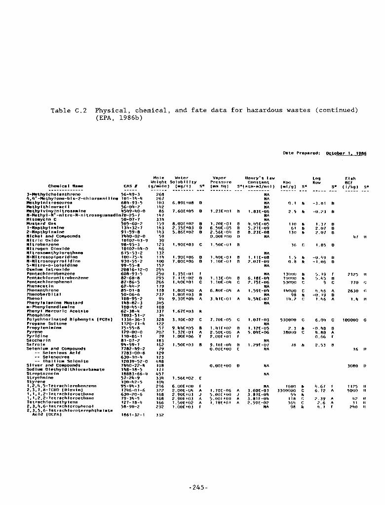
I.
Table C.2 Physical, chemical, and fate data for hazardous wastes (continued) (EPA, 1986b)
I-
- Ostn Prepared: October 1. 1966
Chonlca I Nnme C
3-Methy IchoInnthreno 56-49-3 4,4 ' -Me t hy 1 one-b I s-2-ch I oronn I I I ne 10 1 - 1 It-t i Me thy In I t rosotirca Methyl t h l o u r s c l I ~6-Oh-2
4549-40-0
I-
$84-93-5
Methy I v l ny In I t rossn lne N-Methyl-N'-nltro-N-nltrosoguansdln70-25-7 H l t o n v c l n C 50-07-7 Musts id Cns 1 -Nap thy I nm I ne 2-Nnpthylnnlne N icke l and Compounds N l t r l c Oxlde N I t robenzone N l t rogcn Olox ldo Nltrosomolhylurethsne N-N l t rosop lpe r ld lno N-N l t rosopy r ro t l d lno 5-141 t ro -o - t o l u l d Ine Osmium Tetrox lde Pocctsch lnrobcnzcnc Pcntschloronl trobenzene Pentsch loropheno I Phenscet In Phennn threno Phenoba r b I t n 1 Pheno I Pheny 1 a Ian lne Musts r d m- Phony 1 ened I am I ne Phenyl Mercur lc Acetste Phosphlne Po 1 ych l o r I nn tod 6 lpheny I s ( PCBs) Propsne SUI tone Propylenlmlne Pyreno Pyr I d I ne Sncclca r I n sa r ro l e Selenlun and Compounds -- Selenious Acld -- Selenoilrea -- l h s l l l u m So len i re SI l v e r end Conpotids Sod Iun 0 I e thy I d I th lacs rbnas t e S t reptozoc In Strychnine Styrene 1.2.4.5-let rschlorobenzene 2.3.7,8-TCOO (O lox ln ) 1,1,1,2-le t rsch l oroe thnne 1,1,2,2- l o t rachloroethsne l e t rsclr l o roe thy I ene 2,3,4.6-1etrnchlorophenol 2 .3,5,6- letrechloroterephthslste
Acld (OCPA)
505-60-2 1 311-32-7 91-59-1 WIO-02-0 10102-43-9 98-95-3 10 102- 4 4 - 0 615-53-2 100-79-4 9111-55-2 99-55-8 20816-12-0 608-93-5 82-68-8 87-86-5 62-40 - 2 05-01-8 50-06-6 108-95-2 148-82-3 10@-45-2 62-3R-4 7803-51-2 1336- 36- 3 1 120- 7 I - 4 75-55-8 129-00-0 110-86- 1 81-07-2 94 - 59- 7 7782-49-2 770 3-00-8 630- 10-11 12019-52-0 7440-22-4 148-18-5 18883-66-4 57-2rr-9 I on- 11 2- 5 95-94- 3 1746-01-6 630-20-6 79-34-5 127-16-11 58-90-2
1861-32-1
260 26 7 103 I42 86
1117 3311 157 1 I1 3 1 !I 3 59 3 0
123 116
132 1 1 4 IO0 152 254 250 295 266 179 1 7 8 232
94
1 08 337 3 4 328 122 57
202 79 183 162 79
129 123 408 I08 171 457 334 1 no 216 322 1 G8 168 166 232
332
305
6.89E4O8
7.60E405
8 . 0 0 ~ 4 0 2 2.35E403 5.86€+02
1.90€+03
1.35E-01 7. I l E - ( I Z I . I I O E + ~ I
i . 0 0 ~ 4 0 0 1 .00E403 9 . 3 0 E 4 0 4
1.67C403
3.10E-02
9.44E405 1 .32E-UI I . OOE406
1.50€+03
1.56E402
6.0Ot400 2. OOE -011 2.90E403 2.90L403 1.50€+02 1.00E403
D
D
D D D
C
D n
f 0 C
A 0 A
K
C
6 A f
8
E
f A J n A f
Vapor Pres si8 r e (mm I lq l S
1 . 2 3 E 4 0 1
1 .70E-01 6.50E-05 2. 56 t - 0 1 1 0. 0 0 ~ 4 0 0
1.50E-01
1 . 4 0 L - 0 1 I . ioc-ui
1 . 1 3 E - 0 4 1. I O E - 0 4
6.80t-04
3 . 4 1 E - 0 1
7. IO€-05
I .(I 1 t t n ? 2.50C-UG 2 . 0 0 ~ 4 n i
0.00~400
I . 7OC-06
5. OOL 400 l+ 7 R E 4 O I
5 . ooc 4110
0
D D D 0
0
D n
D C
A
A
C
0 A f
D E
0
A J A A
I lenry's t a w constnnt
Inta-m3/mol) -------- NA NA MA NA
1.83t-06 NA NA
4.~15t-05 5.2 l t - 0 9 8.23t-08
NA
HA 1 . I I€-08
NA
HA 6. I8E-04 2.75C-06
NA
2.07t-n9
1 .59E-Il4 NA
4.54t-07 NA
1 .O7€-03 MA
1.12E-05 5. Oh E -06
NA 1.29E-07
NA
MA
NA
NA 3.60E-03 3.0 I€-04 3 . 8 1 E - 0 4 2.59E-02
MA
Koe ( m l / g ) - - -___
0 . I
2.5
1 10 61
130
36
1.5 n.8
13lIlJll 1 WlI0 5 300U
I linuu 98
1 4 . 2
5300110
2.3 3RUOO
10
1600 3 3onnun
5 P I I 1 0 360 98
S. _--
k
k
k k k
C
k k
k k C
C k C
C
k C
k
k C k c c k
- 3 . R 1
-0.73
1.37 2.07 2.07
1.R5
-0.49 - 1 .06
>. l Y > . t i5
5
4 . 116 -0. l Y
1 ,116
6.04
-n. IO 'I. 80 0.66
2.53
4.67 6. 72
7.19 7 .6 4 . 1
n
6
n U D
0
n n
r D C
A 0 A
C
0 A f
8
f A
A A F
4 7
2125
7 7 0
2630
1 . 4
100000
16
3080
1175 50110
It 7 .3 I
240
II
II
c r.
II
G
I1
IJ
II II
I1 II II
- 245 -
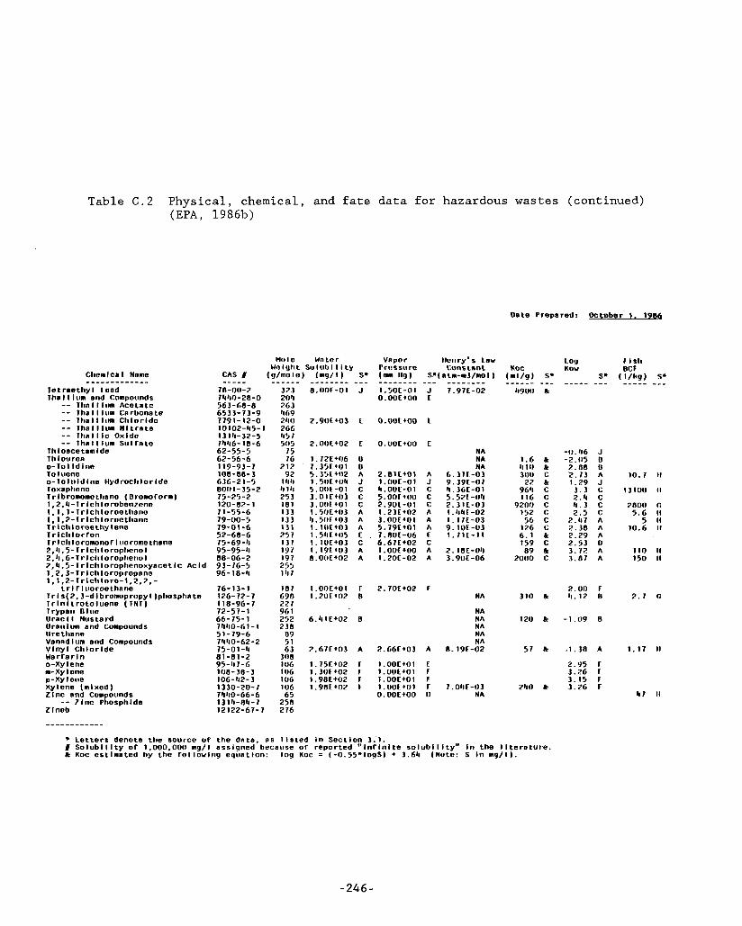
Table C . 2 Phys ica l , chemical, and f a t e da ta f o r hazardous wastes (continued) (EPA, 1986b)
Oate Prepared: *Lobober 1. 1986
Clremica I Name _------------ Tet rae thy l Lead Tha I I I urn and Compounds -- T I t a I I lun Acotam -- I h a l I l u m Carbonate -- IhaI I l u m Chlor ldc -- I h a l l l u m N l t r s t e -- T h n I l l c Oxido -- I h a l l l u n Su l ra tc Thloacetanlde Th Iouroa 0-101 Id l i re To I uanc 0- l o I ii I d I ne I l ydroch lo r Ida Ioxoplicna T r I b romoma t ha ne ( 0 romo ro r m ) 1,2.4-T r lclr lorobenzene 1,l. 1 -1 r I c h lo roe tliano 1,1,2-TrIchloroethane 1 r I clr l o roe thy leno T r I clt l o r r o n 7 r l c l i I oromonor I uoromethane 2,11,5-lrlclt lorophenol 2.4.6-1 r l c l r I oroplieno I 2.4.5-Ir lchlorophenoxyacet I c Ac I d 1,2,3- T r I ch I oropropnne 1,1,2-~r lchloro-1.2,2,-
t r I r I uoroe thane Irls(2.3-dlbronopropyl)phosphate T r l n l t r o t o l u e n e ( T N T ) Trypan OIue Vracl I Mustard Uranium and Compounds U r e t l ia ne Vanadlun and Compounds V lny l Ch lor lde Ua r r a r I n o-Xylene m-Xylene p-Xylene Xylene (n l xed ) Z lnc and Compounds
Zlneb -- Z lnc Phosphlde
CAS I
78-00-2 7450-28-0 563-68-8 6533-73-9 7791-t2-0 10102-h5-1 131tt-32-5 7446-18-6 62-55-5 62-56-6 119-93-7 108-88-3 636-21-5 800 1-35-2 75-33-2 120-82- I 71-55-6 79-00-5 79-01-6 52-68-6 75-69-11 95-95-4 88-06-2 93- 16-5 96- 18-18
76-13-1 126-72-7 118-96-7 72-57-1 66-75- 1 7450-61-1 51-79-6 71140-62-2 75-01-4 81-81-2 95-47-6 108 - 3 8 - 3 106-42- 3 1330-20-7 7440-66-6 13 14-84-7 12122-67-7
----- 323 204 263 ,169 2110 266 457 505
15 76
212 92
11111 11 14 253 181 133 133 131 257 1 3 7 197 197 255 14 7
107 690 227 96 1 252 238
09 51 63 308 106 I06 106 106 65 258 276
8 . O O E - 0 1 J
2.90E403 E
2 . 0 ~ ~ 4 0 2 E
1.72E406 U 7.35FW1 0 5 . 35C4112 A 1.5llL+O4 J 5.00E-01 C 3 . 0 l E + t ) l c J.OOE+OI c 1.5UE+03 A t l . 5 0 C + O l A 1. 102+03 A 1.5hC405 E 1.lUE+O3 C 1.19C+03 A 8 . 0 ~ ~ 4 0 2 A
1 . 0 0 ~ 4 0 1 r 1 . 2 0 ~ 4 0 2 o
6.41E402 B
2.67Et03 A
1.75C+02 i
1.98EW2 i 1.98E402 F
1.30~402 r
Vnpor I lc i i ry ' s Law Frr?ssure (mm 119) S*(a~m-m3/mol)
Cons t s n t
0 . 0 0 ~ 4 0 0
O . U O E 4 0 0
2.01~401 1. nvE-o i 4 . OUE - 0 1 5.OOL400 2.9UC-01 1.23E402 3. ooc+o I 5.79C401 7. RUC-UL 6.67E402
1.20C-02 1.00c400
2.70C402
2.66E403
1 . 0 0 E t 0 1 1. UOEIO I 1.00~40 I 1.00~401 0.00~400
J t
E
E
A J C C C A A h E C A A
r
A
E i i i U
NA NA NA
6.372-03 9.39E-07 4.36f-01 5.52L-011 2.31t-03 1 . w E -02 1. I 7 C - 0 3 9 . l O t - 0 3 1. I lE-11
2. I8L-Oh 3 . 9 ~ - 0 6
NA
NA NA NA HA NA
8.19E-02
7.04E-03 HA
s9vu
1.6 11 1 I) 3 0 0 22
96'1 I I 6
9200 152 56
126 6.1 159 89
2000
3 10
120
57
2110
k
k k C k C C C C C c k C k C
k
k
k
k
-0 .06 -2.115 2.08 2.73 1.29 3.3 2 . 4 4 . 3 2.5
2.47 2.38 2.29 2.43 3.72 3.87
2.00 11.12
-1.09
. I . 38
2.95 3.26 3. 15 3.26
J 0 U A J C C C C A A A 0 A A
i 0
0
10.7 II
13100 II
2800 G 5.6 II
5 II 10.6 II
I10 II 150 11
2.7 C
1.17 II
47 I1
' L e t t e r s denote the source of the data. a s l t s t e d In S e c t l o t 3.1. I S o l u b l l l t y or 1.000.000 ng/l assigned because or reported l n r l n l t e s o l u b l l l t y " In the I l t e r a t u r e . k KOC es t l na ted by the ro l l ow lng equat lon: log Koc = (-0.55.10gS) + 3.64 (Note! S In m g / l ) .
-246 -
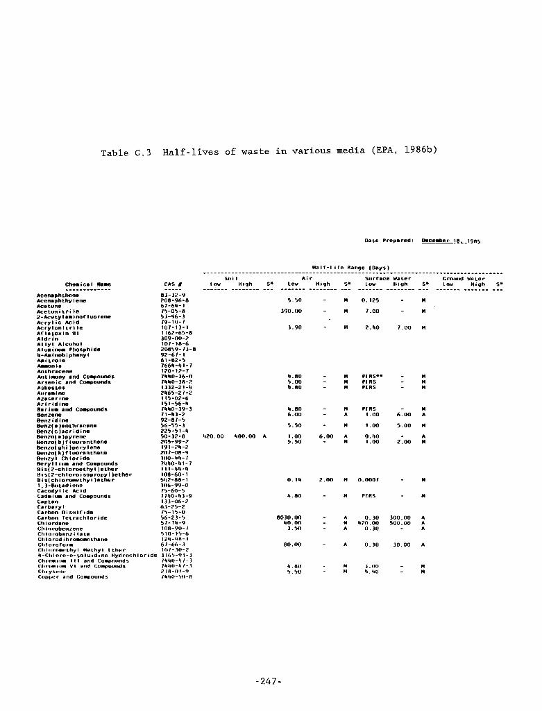
Table C . 3 Half-lives of waste in various media (EPA, 1986b)
Chemical Name -------__---- Acenaph ttiene Acenaphthylene Acetone Ace ton i t r i l e 2-Acetyl8minofluorene Acry l i c Acid Ac ry lon i r r i l e A f l a tox in B i A ld r i n A I l y l A I C O I I O I A I um irwu Phosph Ids 4-Aminobiphenyl Amitrole -nia Anthracene Antimony 8nd Compounds Arsenic 8nd Compounds Asbestos Aiiraml ne Azaserine A z i r i d i ne 08 r i iim and Compounds Benzene Benz i d I ne Ben.?(. )anthracene Benz( c )ac r i d i ne Benzo(a )pyrene L4enzo( b f luoranthene Benzo(ghi )perylene Benzo( k 1 f I uoranthene Benzyl Chlor ide Be r y I I i tam and Coupoiindr Bis(2-chloroethyl lether B i s 2-ch I or0 i sop ropy I )e the r Bis(chlorolethy1)ether 1.3-Butadiene Cacodylic Acid Cadmiua and Coapounds CapLan Ca rba r y I Ca rbnn O i sii I f tde Ca rbori le r rach lo r ide Chlordane Cl i lnrobeiizene CIi lurobenz i I a L e Clt I o rod I h rowmethane CII I tBr"r,>,-
Hal f - l i f e Range (Days) . . . . . . . . . . . . . . . . . . . . . . . . . . . . . . . . . . . . . . . . . . . . . . . . . . . . . . . . . . . . . . . . . . . . . . . . . . . . . . . . . . . . . Crouiid WaLcr Soi I A i r Siirface WaLer
Lm High S* Low High So L w High 5. lm High So _ _ _ _ _ _ _ _____- - - --- ------- -------- --- ------_ -------- --- --- - -_- - _ _ _ _ _ _ _ _ _ ----- 83-32-9 208-96 - 8 5.50 67-64- 1 75-05-8 53-96-3 79- IO- 7 107-13-1 1167-65-8 309-00-2 107-18-6 20859- 73-8 92-67-1 61-82-5 766b-41-7 120- 12-7 7440-36-0 7440- 38-2 1332-21-4 2465-27-2 115-02-6 151-56-4 7040-39-3 7 1-43-2 92-87-5 56-55-3
- M - M 0.125
390.00 - M 7.00 - M
- M 2.40 7 . 0 0 M 3.90
- M PIRS.. - M 4.80 - M - M P t H S 5.00
4.80 - M PCHS - ? I
b . 8 0 - M P r R s - I ( 6.00 - A 1.00 6.00 A
- M 1.00 5.00 M 5.50 225-51-4 50-32-8 420.00 480.00 A 1.00 6.00 A 0.40 - A 205-99-2 5.5u - M 1.00 2.00 M 191-24-7
100-44-7 7440-41-7 1 11-44-4 108-60-1 542-88- 1 106-99-0 7 5 - 61) - 5 7740-43-9 13 3-U6-7 63-25-2 75- 15-0 56-23-5 5 I- 74 -9 108-90- I 510- 15-6
67-66-3 I O 7 - 30-7
20 7-08-9
1741-4n- I ~ . . Ch lnrnmethy I Helliyl 1 ther 4 - C h I o rv-0- LO I u i d t ne Hyd rocti I o r i de 3 165-9 3 - 3 Chvnmiiim I I I arid Cumpnunds 7ltLlJ-~l/-3 (:la r o m I im V 1 and Compuuiids 74411-ti I - 3 ct, r ysenc 2 in-ni-y Copper arid Compounds r u t ~ i t - ~ i - n
0.14 2.00 M 0.0007 - M
4.80 - M PERS - M
8030.00 - A 0 . 3 0 3oo.00 A 40.00 - M 470.00 500.00 A 3.50 - A 0.30 - A
- A 0.30 30.00 A 80.00
4.nu - n 3.011 - M 5.50 - M t i . t i I J - M
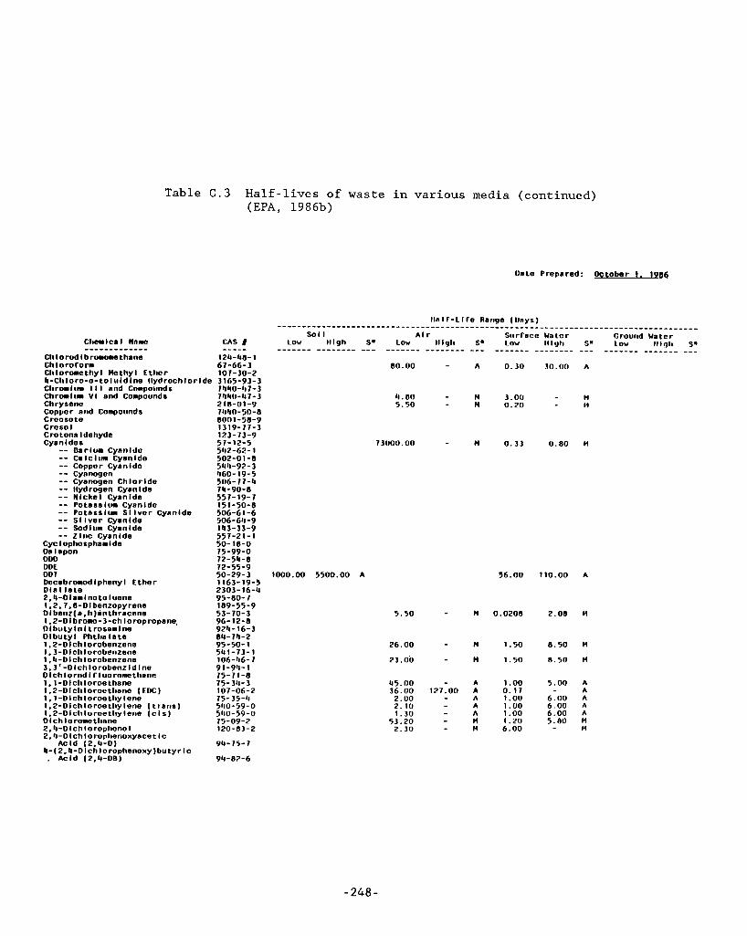
Table C . 3 Half-lives of waste in various media (continued) (EPA, 1986b)
OaLe Prepared: October I . 19Qtj
Chemical Nnm' CAS I ------------- - - - -_ Ch io rod i b romow thane 124-118- I Ch I orororm 67-66-3 Chloromethyi Mothy1 Ether 107-30-2 4-Cl i ioro-o- to lu id lne l lydrochlor lde 3165-93-3 Chromiiim I I I and Compoiinds 14hO-47-3 Chromium V I and COlDOUndS 7(1110-~17-3
2 in-01-9 Chryseno Coppcr arid Compounds Creosote Crosoi Crotona ldeliyde Cyan i dos -- O a r i u m Cynnidc -- Calcium Cyanide -- Coppor Cyanldc -- cyanogcn -- Cyanogen Chlor ide -- liydrogen Cyanide -- Nickel Cyanide -- Potassium Cyanido -- Potassium SI l v e r Cyanide -- S i l v e r Cyanide -- Sodium Cyanlde -- Zirrc Cyanide Cyclophosphamide Da I apon ODD DOL OD1 Oecabromodiphenyl Ether D i e l l a m 2.4-Oiaminotoiuene 1,2,7,8-0i benzopyrene Dlbenz(a,h)snthracene 1.2-Di bromo-3-ch ioropropane, O i b u t y l n i t rosami ne D i b u t y l Phthalate 1.2-Dichlorobenzene 1.3-Dichlorobenzene 1.4-Oichlorobenzene 3.3'-Oichiorobonzldlnc Olch l o rod I r luoronethane 1.1-Dich ioroe thane 1,2-Oich loroethane ( EDC) 1.1 -D I ch 1 oroe thy I ene 1,2-Oichloroe thy I ene ( t rans ) 1.2-0 i ch I o roe thy I ene ( c I s ) D 1 c h I o rome t ha ne 2.4-Oich loropheno I 2,4-0 I ch 1 orophenoxyace t i c
4-(2.4-Dlchlorophenoxy)butyrlc Acid (2.4-0)
. Acid (2.4-08)
i t m i s o l a eon I - 58-9 1319-71-3 123-73-9 57-12-5 542-62- 1 502-01-8 5WI-92- 3 1160-19-5 506-77-4 74-90-8 557-19-7 151-50-8 506-61-6 506-60 -9 14 3- 3 3-9 557-21- 1 50- 18-0 15-99-0 72-54-8 72-55-9 50-29-3 l lG3-19-5 2301-16-4 95-80-7 189-55-9 53- 70- 3 96- 12-0 924- 16-3 84- 711-2 95-50- 1 541-73-1 106 -116- 7 9 1-94- 1 75- 7 1-8 75-34-3 107-06-2 75-35-4 5110- 59 -0 5110-59-0 75-09-2 120-83-2
94- 75- 7
94-82-6
11. 80 - H 3.00 - H 5.50 - H 0.20 - I4
1000.00 5500.00 A
73lJOU.00 - M 0.33 0 .80 H
56.00 1io.00 A
5.50 - M 0.0208 2.08 I4
26.00 - M 1.50 8.50 H
23.00 - H 1.50 0.50 H
45.00 - A 1.00 5.00 A 36.00 127.00 A 0.17 - A 2.uo - A 1.00 6.00 A 2.10 - A 1.UO 6.00 A 1.30 - A 1.00 6.00 A
53.20 - M 1.20 5 .80 H 2.30 - H 6.00 - H
- 248 -
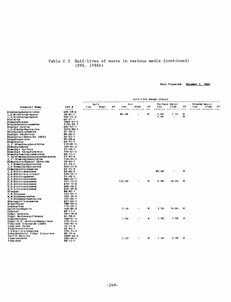
.-"-
A.
Chcmlcnl Nnno ______--_---- Dlchlorophcny I n r s I ne I . 2-Dlcl i lnrooroonnc 1 ; ~ - ~ 1 c h 1 o r o p r o p c n e D l e l d r l n V leooxybutsrie Diethnno In1 trosamlne D l e t h y l Ars lnc 1.2-Dlethylhydrnzlne D io thy ln l t rosnmlne D l c t h y I Plithn I n t e D l e t h y l s t I 1 best r o I ( DES) Dlhydrosn r r o 1 e 0 I me tlion t e 3.3' -Dlmotlioxybcnzld lne Dlmothylamlnc Dlmetlryl Su l fa te D I metliy.l l e rcph t h e I n t c Dlmotlry l nml nonzobenzone 7 l~-Dlmetliylbonz(a)nnthrscene 3: 3 * -Dime th I benz I d Ine Dlmethy Icn rgnnoy l C h l d r Ide 1,l-Dlmothy I hyd rsz I ne 1.2-0 lme t hy I hyd rnz I ne DI IS t hy I n I t rosnm I ne 1.3-Dlnltrobenzene 4.6-Dln l t ro-o-cresol 2.4-01 n I t ropheno I 2.3-Dln l t ro to lucne 2.4-01 n l t r o t o I uene 2.5-01111 t ro to luene 2.. 6-0 In I t roto1 uene 3.11-0 In I t ro t o I uene 01 rroseb 1.4-Dloxnne N, W-Dlpheny I n m i ne 1,2-Dlphenylhydrazlne Dlpropy In I t rosnml ne D l s u i r o t o n Endosul f nn Ep I c h I orohydr l n E thnno I Ethy l Acetnte E thy I Hctl lrncsu 1 fona t e Ethylbenzene E thy l -1 i .h ' -d I ch l o robenz I I a t e Ethylene Olbromlde ( € O B ) Etlrylcne Oxide E thy1 ene t h Iouren 1-Ltlry l -n i t rosouren E thy lph t l rn l y l E thy l G lyco la te f e r r l c Dextran f I uornnt hene f I uo rene
Table C.3 Half-lives of waste in various media (continued) (EPA, 1986b)
Onto Prcparod: October 1. 1'9336
Iln I T-LI r o flange (nays) ________________________________________-----.---------------------------------------
sol I A I r SurCnce Water Crnund Wn1r.r l o w I l l gh S. l o w 111qh S. c n w 1 1 1 ~ ~ 1 l so cow I l i q l l S"
CAS ----- a - _ _ _ _ _ _ _------- --- ------- -------- --- ------- -------- --- ------- ------- - - - 696 - 7n -6 18-87-7 8 V . 00 - H 1. 1 1 0 7 . 7 0 H 511 2 - 7 5 - G 1 .on - I4 60-47- 1 lh6h-53- 5 1116-5'1-7 692-h?-? 1615-80-1 55- 18-5 84-66-2 56-53-1 911-98-6 60-5 1-5 1 ig-go-t i 1211-110-3 17-70-1 120-61 -6 60-11-7 51-91-6 119-93-7 19 - 4 4 - 7 57-1s-14 540-13-8 62-74-9 99-65-0 534-52-1 51-28-5 602-01-7 12 1 - 111 -2 619-15-8 606 -20- 2 610-39-9 88-85-7 123-91-1 122-39-4 122-66-7 621 -611-7 298-011-0 115-29-7 106-89-8 64- 17-5 141-78-6 62-50-0 100-11 1 - 4 5 10- 15-6 106-9 3 -11 75-21-8 96-115-7 759-73-9 84-72-0 90Vh-66-11 206-tlh-0 86- 7 3 - 7
96.00 - w
- n 0.110 in .00 n 1 3 3 . 0 0
- M 3.50 10.8U M 2. 7 0
- A 1.50 7.50 A I . 116
5.50 - n 1.00 2 .00 n
,.-.
-249-
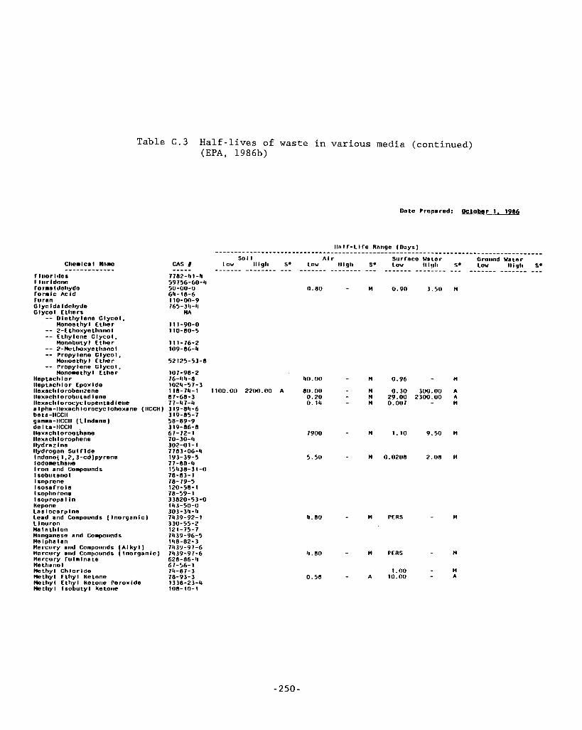
Clienlcal Nnmo ------------- i luor ldor F I iir ldnno Forma Idoliydo Formic Ac id Furan G I yc Ida I deliyde Glyco l Ethers -- D le t l i y leno Glyco l .
Monoe thy1 E t l i e r -- 2-E thoxye thnno I -- Ethylone Glycol , Monobutyl E ther - - 2-Mu L hoxye t Ira no I -- Propylene Glyco l , nonoethyl E t l ie r -- Prbpylerie G lyco l . Monomethyl E ther
l lep tach lo r I leptacli I o r Epoxlde Ilexacli lorobenzono Ilexach I o robu tad i ene llexacli lorocyc lopentadlene a I pha-llexach I o rocyc 1 ohoxane beta-IICCII
Table C.3 Half-lives of waste in various media (continued) (EPA, 1986b)
Date Propared: m g b e r 1. 1984
CAS I ----- 7782-51-h 59756-60-4 50-00-0 64- 18-6 1 io-on-9 765-511-11
NA
0.80 - H u.9n 3.50 n
1 1 1-90-0 110-80-5
111-76-2 109-86-4
52125-53-8
101-98-2 76-04-8 1025-57-3 118-74-1 1100.00 2200.00 87-68-3 77-47-4
(IICCH) 119-811-1 3 19-85-7
gamma-IICCII (L lndane) de l ta-IICCII I lexachloroethane Ilexach 1 orophene llyd rn z I ne llydrogen Su l r l de Indeno(l.2.3-cd)pyrene I odome thane I r o n and Comoounds I sobu tan0 I Isoprene I sosaCrole I sophorone lsopropal In Repone Las l ocarp lne Lead and Compounds ( Ino rgan lc ) L lnuron Ma l a t h l o n Manganese and Compounds Me lpha Ian Hercury and Compounds ( A I h y l Horcury and Compounds ( Inorgan lc ) Mercury F u I n I na t e Methano I Methyl Ch lor ide Methyl E thy l Ketone Methyl E thy l Ketone Peroxide Methyl I sobu ty l Ketone
58-09-9 319-86-8 67-72-1 70- 30-4 102-01- 1 7783-06-4 193-39-5 77-88-4 15438-31-0 78-81-1 78-79-5 120-58-1 78-59-1 33820-53-0 111 3-50-0 303 - 34 -4 7439-92-1 330-55-2 121-75-7 71139-96-5 1118-82-3 71139-97-1 7439-97-6 628-86-11 67-56-1 74-87-3
1138-23-4 108- 10-1 78-93-3
so. 00 - M 0.96 - n
A 80.00 - H 0 . 3 0 lUlJ.00 A 0 . 2 0 - M 29.00 2300.00 A
- M 0.14 - M 0.007
7900 - M 1.10 9.50 M
5.50 - n o.0208 2.08 n
4.80 - M PERS - M
4.80 - M PERS - M
i .no - M 0.58 - A 10.00 - A
-250-
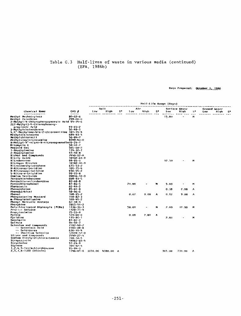
Table C . 3 Half-lives of waste in various media (continued) (EPA, 1986b)
Uatc Prepared: W r 1. 19-86
Iln 1 r-1 I r e Rnnge ( ~ n y s ) . . . . . . . . . . . . . . . . . . . . . . . . . . . . . . . . . . . . . . . . . . . . . . . . . . . . . . . . . . . . . . . . . . . . . . . . . . . . . . . . . . . . . Siirrnce Water Ground Wnlcr sot I A I r
C l i e n l cn 1 Nnne Low I l lgh S" l o w I l l q l r Sa l o w Illqlr 5" Low I i l q l r s* ------------- CAS ----- a _ -_- - - - -------- - - - - - - - - - - - - - _ _ _ - - - -_ _ _ _ _ _ _ _ _ _ _ _ - _ _ _ _ _ _ _ _ _ _ _ _ _ _ _ _ _ _ _ _ _ _ _ Methyl Mclhncry ln le an-62-6 15.00 - I 4 Motliy I rn ra t l i I on 290-nu-n 2-Mcthy I -11-cliloroplrcrioxyncct IC AC I d 911- 711-6 2( 2-Mc thy I ) -ti-Ch lorophcnoxy-
p r o I o i i l c Acld 93-65-2 J-Mcl.l),y I chu 1 antlireire 56-119- 3 11. It' -kcLliy lenc-b I s-2-ch 1 oronn I I I ne 101 - 111-11 Hetliy In1 t rosniircs 6811-93 -5 Hc t l ry I t l r Io t i rec I I 56-011-7 Flc thy1 v I nyl n I t rosnnine 45'I9-'lU-0 N-M@LIivI-N'-nl t ro -N-n l trosoa~ianndln70-25-7 Mltomy;ln C Mustard Gas 1 -Nnplliy I nn I ne 2-Nnptliylnnlne N lcke l and Compbunds N l t r l c ox ide Nl t robcn7rne N l t rogcn I ) lox lde N I t rosomclliy I nrcthnne N-NI t rocop lpc r ld lnn N-MI t rosopy r ro l Id l r ie 5 -N l t ro -o - to lu ld lne Osml urn l e t rox I de Pentach 1 orobenzene Pentachloronl t robenzone Pentnchlorophenol Phenacet In Phensn th rene Plienoba r b I t s 1 Pheno I Pheny la I an Ine HIIS t s r d n-fhenylencdlamlne Phenyl Mercur lc Acetrrte Plrosph I ne Poly' t i t o r Inn ted Blphenyl s ( PCBs) Prop?, P Sir1 tone Propy I en Imlne Pyrene Py r I d I ne Snccharln s a r r o l e Se I en I urn nnd Compounds - - Selenloiis Acld -- Srlenorirea -- l h n l I l i i m S c l c n l t e S I l v r r and Cornpoitrids Sod Iiin D l r t t r y l d I tblocnrbnrna r e St reptoznc ln Strychir lne Styrene 1 . 2 . 4 . 5 - l e t r a c h l o r o h e n ~ e n r 2 . 3 . 7 . 8 - I C 0 0 (O lox ln )
50-11 i - 7 505-60-2 1311-32-7 91-59-8 T W U - O Z - O 10102-43-9 98-95-3 iu I 02-1111-n 615-53-2 I00 - 7 5 -0 930-55-2 99-55-8 20816-12-0 608-93-5 82-68-8 81-86-5 62 - 1118 - 2 85-01-8 50-06-6 lU8-95-2 IIlO-82- 3 100-45-2 62- 38-11 7803-51-2 1336-36-3 I 120-7 1-4 75-55-8 129 -00 - 0 110-06-1 81-01-2 911-59- 7 7 7 82- h 9 - 2 7 783 -00-8 630-in-11 12039-57-0 7 11110-27 - 11 100-10-5 18803-66-4 57 - 211 - 9 100- 02- 5 95-911-3 1746-01-6 3650.00 4 3 8 0 . 0 0 A
-I
- 2 5 1 -
17.51) - I4
21 .OO - w 5.00 - M
0 . 3 8 2.00 A
0.62 9.00 A 0.62 9.UU A
- H 2.00 17.90 M 58.00
0 . 0 8 7.00 A 2 .00 - I 4
365. ou 7 3 0 . on A
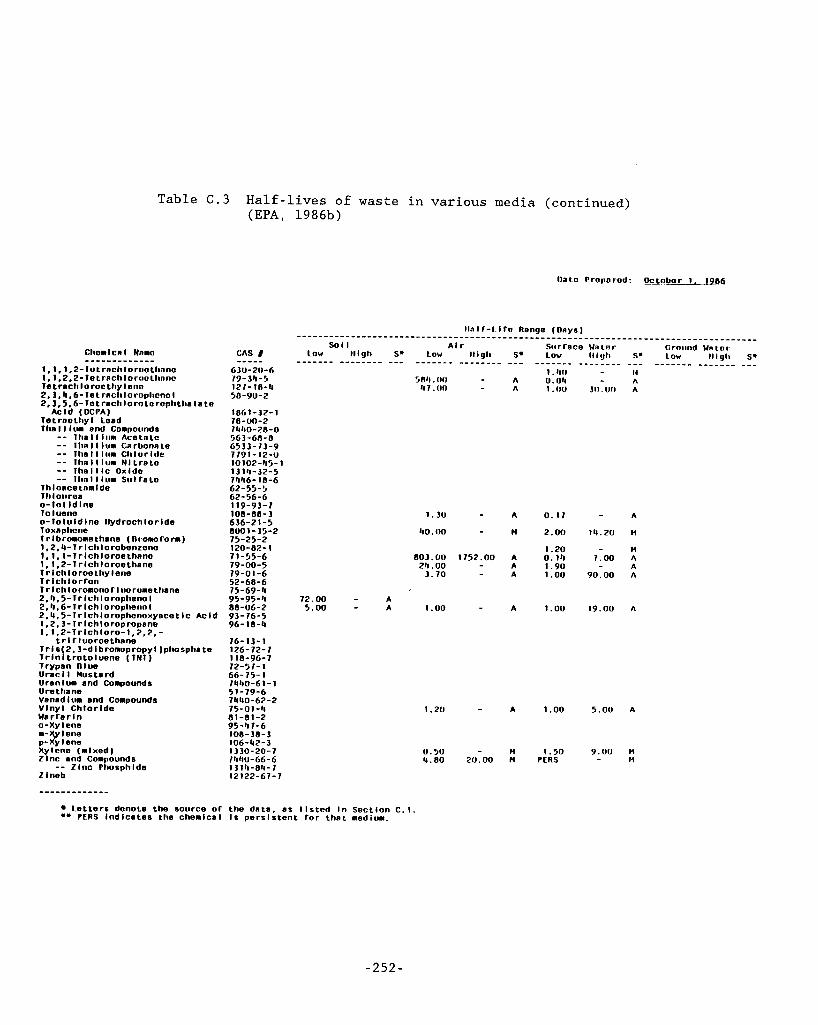
Table C.3 Half-lives of waste in various media (continued) (EPA, 1986b)
Ontc Prcporod: OcAnbor 1 . 1986
Chcmlcnl Nnmc ------------- 1, 1, 1.2-IutrnchloroctI inno 1,1.2,2-1etr~chlorirclhnnc I e t r n c l ~ I o r o c t l ~ y Iorrc 2,3,4.6-1et rnc11IoroplicnoI 2,3,5.6- 10 t rach I o r o t o rcphtha I a t e
Acld (OCPA) TetrocLl iyI Load fhn I I i i i m and Compoiinds -- l h n l I liin AcetnLc -- I l i n I I Iun Cnrbonnre -- I h n I I I i im Ch lu r ldc -- I h n l l l u m N l t r n t o -- I h n l l l c Oxldc -- 1tinI1ium s i t i r a t c I h I once tnn I de Ih I oiiroa o -To l l d lne Io I ueno 0-10 I u l d I ne llydroch l o r Ida Toxnphcne I r I bromome t hane ( nromo rom ) 1.2.4-Ir lchlorcbonzcno 1.1.1-Ir lchloroethnnc 1 , 1 ,2-I r I ch I orce t hane I r I ch I o roe thy I ens I r l c h l o r r o n I r lchloromonor I uoronethane 2,11, 5 - I r I c h I oropheno I 2.4,6-1rlchloropl1enol 2,4,5-T r lchlorophcncwyacet I C Ac I d 1,2.3-I r Ict i loropropane 1.1.2-Irlchloro-1.2.2,-
t r l r Iuoroethnne T r I s( 2, 3 -d I b ro iop ropy I )phospha t e I r l n l t r o t o l u e n e ( T N I ) I r ypan Olue Uracl I Mustard Uranlun and Compounds Urethane Vanadlum and Compounds V lny l Chlor lde Wa r r a r I n 0-Xy lene
Xylene (n l xed ) Zlnc and Conoounds
;3$%
1861-32- 1 7 8- vo-2 111110-28-0 563-6R-0 6533-73-9 7791-12-V 10102-ll5- 1 1 3 1 I1 - 32- 5 75h6-l8-6 62-55-5 62-56-6 119-93-7 108- 88 - 3 636-21-5 800 1 - 35 - 2 75-25-2 120-82- 1 71-55-6 79-00-5 79-01-6 52-68-6 75-69-11 95-95-11 72.00 - A 80-VG-2 5.00 - A 93-76-5 96-18-4
1 .vo - A 1.00 19.0V A
76-13-1 126-72-7 118-96-7 72-57-1 66-15-1 74110-61-1 51-79-6 7440-62-2 75-0 1 - 11 8 1-81-2 95 -11 7-6 108- 38-3 1V6-42-3 1330-20-7 755O-66-6 1 3 111-811 - 7 12122-67-7
1.3V - A 0.17 - A
llO.00 - n 2.00 i11.20 n
1.20 - n 803.00 1752.00 A 0.111 7.00 A 2(1.00 - A t a n A
3.70 - A
1.20 - A 1.00 5.0V A
0.50 - n i . 5 n 9.00 H 4.80 20.00 n PERS - H
L e t t e r s denote the soiirce o r the dnta. as I l s t e d i n Section C . l ** PCRS Ind l ca tes the chemlcnl I s p e r s i s t e n t Cor t hn t medium.
- 2 5 2 -
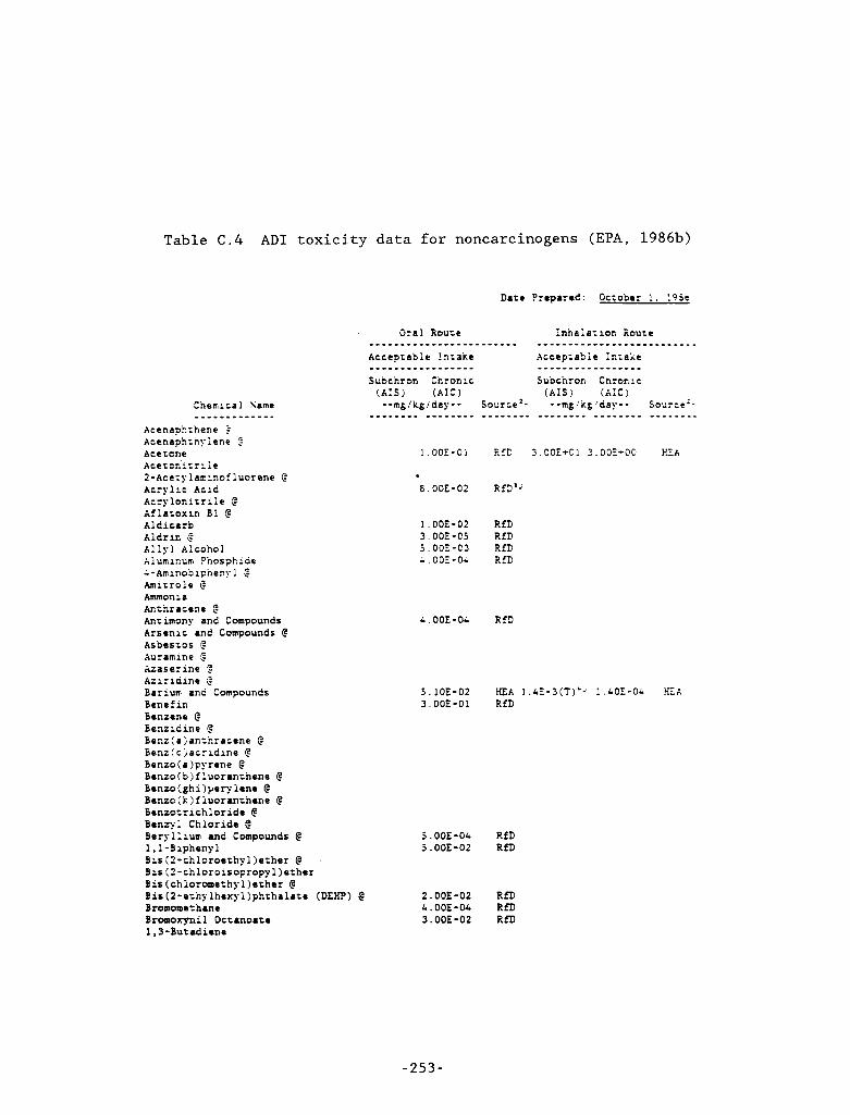
e-
-
.._”
. --
Table C . 4 AD1 toxicity data for noncarcinogens (EPA, 1986b)
O r a l Rouze
Acceprable Lnr3ke - - - - - - - - - - - - - - - - -
Dare Prepared: Ocrobcr 1. 1930
Subcnron Chronic ( A I S ) (AIC) --m&/k&/day-- Source’- ---.---. - - - - _ _ _ _ _ _ _ _ _ _ _ _ Chemical kame - - - - - - - - - - - - -
Acenaphzhene ? Acenaphrhpiene f Acetone Aceron’izri le ?-Ace_ylaminofluorene I? Acrylic Acid A-rylonitrile e Aflazoxm B1 S Aldicarb Aldrin C Allyl Alcohol Aluminum Pncsptide A-Aminobiphenyl CS Amirrole G .Ammonia hznracene C: Anrimony and Compounds Arsenic and Compounds @ Asbesros @ Auramine C. Azaserine F Aziridine 2 Barium ana Compounds Bene f in Benzene @ Benzidine @ Be:.z (a)anzhracene C: Benz(cjacridine @ Benzo(6)pyrene @ Benzo(bjfluoranrhene Q Benro(ghi)perylcnc @ Benzo(k]fluoranrhcne @ Benzozrichloridc Q Benzyl Chloride Q Beryllium and Compounds @ 5.00E-01 RfD 1,l-Biphenyl 5.00E-02 RfD Bis(2-ch1orocrhyl)erher @ . Bis(2-chloroisopropy1)ether Bis(chloromechj.l)czhrr @ B is ( 2 -erhy 1 hexy 1 ) phrha late (DEW) Q 2.00E-02 RfD Bromomethane L.OOE-OL RfD Bromoxynil DCtAnOACe 3.OOE-02 RfD 1,3-Bur~diene
1.00E-01 RCD 3.00E+G: ?.OOE+OC Hfk
8.OOE-02 RfD’-
] .DOE-02 RfD 3.001-Cj RfD 5.00E-C3 RfD - . O O E - 0 - RfD
A.OOE-OL RfD
5 . 1 0 E - 0 2 E A 1.4E-3(f)” 1 .kOE-O4 HEA 3.001-01 RfD
- 253-
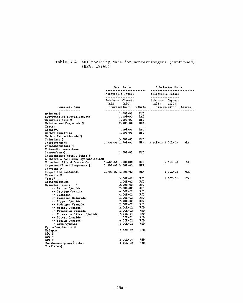
Table C.4 AD1 toxicity data for noncarcinogens (continued) ( E P A , 1986b)
Chemical Same - - - - - - - - - - - - - n-Butanol 1.00E-01 Butylprhalyl Butylglycolate 1.OOE+OO Cacodylic Acid @ 1.00E-02
Captan Carbaryl 1.00E-01 Carbon Disulfide 1.006-01 Carbon Tetrachloride @ Chlordane @ 5. OOE-OS Chlorobenzene 2 .70E-01 2 .706-02 Chlorobentilate @ Chlorodibromomethane Chloroform @ 1.00E-02 Chloromethyl Xcrhyl Ether @ L-Chloro-o-toluidine Hydrochloride@
Cadmium and Compounds @ 2.90E-0ri
Chromium 111 and Compounds Chromium VI and Compounds @ Chrysene @ Copper and Compounds Creosote @ Cresol Crotonaldehyde Cyanides (n.0.s. I ''
Barium Cyanide Calcium Cyanide Cyanogen Cyanogen Chloride Copper Cyanide Hydrogen Cyanide Nickel Cyanide Potassium Cyanide Potassium Silver Cyanide Silver Cyanide Sodium Cyanide Zinc Cyanide
Cyclophosphamide @ Dalapon DDD @ DDE @ Dm @ Decabromodiphenyi Ether Diallate @
l.LOE+Ol 1.00E+00 2.5OE-02 5.00E-03
3 .70E-02 3.70E-02
5.00E-02 1.00E-02 2.oo.E-02 7.00E-02 L.00E-02 (r.00E-02 5.OOE-02 7.OOE-02 2. DOE-02 2.OOE-02 5.00E-02 2.OOE-01 1.00E-01 (r . OOE-02 5.00E-02
8 . DOE-02
5 . OOE-OI 1.00E-02
RfD RfD RfD E A
RfD RfD
RfD E A 5.30E-02 5.7OE-03 HEA
RfD
RfD HEA
E A
RfD RfD RfD RfD RfD RfD RfD RfD RfD RfD RfD RfD RfD RfD RfD
RfD
RfD RfD
j.lOE-03 HEA
1.00E-02 H E A
1.00E-01 HEA
-254-
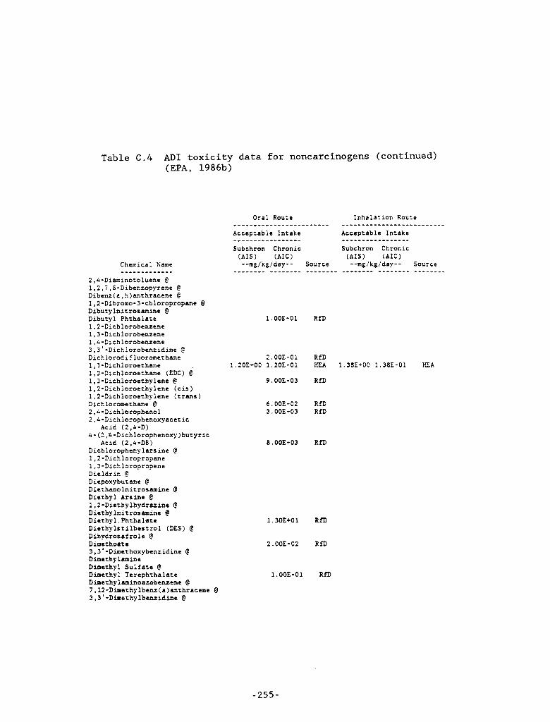
.--
Table C.4 AD1 toxicity data for noncarcinogens (continued) (EPA, 1986b)
7
r ...
Chemical Same - - - - - - - - - - - - - 2,L-Diaminotoluene @ l,?,i,S-Dibenzopyrene @ Dibenz(6,h)anchracene C 1,2-Dibrorno-3-chloropropanc @ Dibutplnitrosamine @ Dibutyl Phthalate 1.2-Dichlorobenzene 1,3-Dichlorobcnzene I,&-Dichlorobenzene 3,3'-Dichlorobenzicine C Dichlorodifluoromerhane 1,l-Dichloroerhane 1.2-Dichloroethane (EDC) @ 1,l-Dichloroerhylene @ 1,2-Dichloroethylene (cis) 1,2-Dichloroerhylene (trans) Dichloromerhane @ 2,L-Dichlorophenol 2,L-Dichlorophenoxyacetic
Acid (2,&-D) L-(2,%-Dichlorophenoxy)butyric
Acld (2,L-DB) Dichloropheny larsine @ 1,2-Dichloropropane 1,j-Dichloropropene Dieldrin @ Dicpoxybutane @ Dierhanolnitrosamine @ Dierhyl Arsine @ 1.2-D~erhylhydr6zine P Dicrhplnirrosamine @ Diethyl.Phthalate Dierhylsrilbestrol (DES) @ Dihydrosafrole @ Dimerhoate 3,3'-Dimerhoxybcnzidine @ Dimethy lamine Dimcrhyl Sulfare @ Dimerhyl Terephthalate Dimcrhylaminoazobenzene @ 7,12-Diaethylbenz(a)anthracene @ 3,3'-Dimethylbentidine @
1.00E-01 RfD
2.00E-01 I.?OE+OD 1.206-01
9 .OOE-O3
6.00E-02 3.00E-03
8.00E-03
RfD HEA 1.38E+D0 1.38E-01 H L A
RfD
RfD RfD
RfD
1.30E+01 R f D
2.00E-02 RfD
1.OOE-01 RfD
-255 -
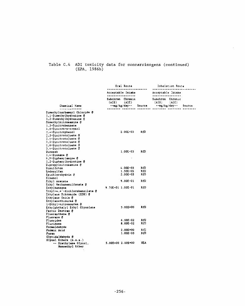
Table C.4 AD1 toxicity data for noncarcinogens (continued) (EPA, 1986b)
Chemical Kame
Dimethylcarbamoyl Chloride @ 1,l-Dimethylhydrazine @ 1,'-Dimethylhydrazine F Dimethylnitrosamine @ 1,3-Dinitrobenzcne ~,6-Dinirro-o-cresol 2.;-Dinirrophenol 2,3-Dinitrotoluene @ 2.A-Dinirrotolucne @ 2,j-DiniKrotoluene !? 2,6-Dinierorolucne @ 3 ,A-Dinitrocolusne !? Dinoseb I,&-Dioxane @ K,H-Diphenylamine @ 1,Z-Diphenylhydrazine @ Dipropylnitrosarnine @ Disulfoton Endotu 1 fan Epichlorohydrin Ce Ethanol Ethyl Acerare Ethyl Yerhanesulfonate @ Ethylbenzene Ethpl-&,4' -d ichlorobcnzi latc @ Ethylene Dibromide (EDB) @ Echylene Oxiie @ Ethylenerhioutea @ 1-Ethyl-nitrosourea @ Echylphchalpl Ethyl Glycolate Ferric Dextran @ Fluoranthene @ Fluorene F F luoridcs Fluridone Formaldehyde Formic Acid Furan Glycidaldehyde @ Glycol Ethers (n.o.s.1 -- Diethylene Glycol,
Honoethyl Ether
- - - - - - - - - - - - -
2.00E-03 RfD
1.00E-03 RfD
&.WE-03 RfD 1.fOE-05 RfD ?.00E-03 RfD
9.00E-01 RfD
9 . iOE-01 1.00E-01 RfD
3.00EM0 RfD
6.00E-02 RfD 8.OOE-02 Rf;,
2.00EM0 R S 1.00E-03 RfD
-256-
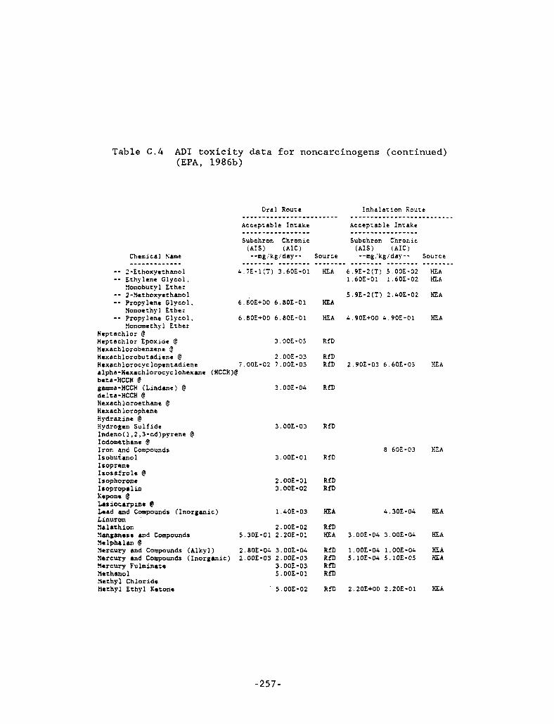
" .
c
Table C . 4 AD1 toxicity data for noncarcinogens (continued) (EPA, 1986b)
I-
-_
-- 2-Erhoxyerhanol L.iE-l(T) 3.60E-01 -- Ethylene Glycol, -- Z-!Jethoxyerhanol -- Propylene Glycol, 6.80E+00 6.80E-01
- - Propylene Glycol, 6.80E+00 6.8OE-01
tlonobutyl Ether
tlonoechyl Ether
tlonomerhyl Ether Heptachlor @ Heptachlor Epoxide B 3.00E-05 Hexachlorobenzenc 2 HexachloroburadLene @ 2.00E-03 Hexachlorocyclopencadiene i.OOE-02 7.OOE-03 alpha-Hexachlorocyclohexane (HCCH)@ beta-HCCH @ gmms-HCCH (Lindane) @ 3.006-04 delta-HCCH @ Hexachloroethane @ Hexachlorophene Hydrazine @ Hydrogen Sulfide 3.00E-03 Indeno(1.2.3-cd)pyrene @ Iodomcthane @ Iron and Compounds Isobuianol 3.OOE-01 Isoprene Isosafrole @ Isophorone 2 . OOE - 01 Isopropalin 3.OOE-02 Keponc @ Iasiocarpinc @ G a d and Compounds (Inorganic) 1 .LOE-03 Linuron tlalarhion 2.00E-02 Xanganese and Compounds 5.30E-01 2.20E-01 Yelph61an @ Ycrcury and Compounds (Alkyl) 2.80E-OL 3. OOE-OL ?lercury and Compounds (Inorganic) 2.006-03 2.OOE-03 Yercury Fulminate 3.OOE-03 Sethano1 5.00E-01 %thy1 Chloride Methyl Lchyl Ketode 5.OOE-02
E A
E A
HEA
R f D
R f D R f D
R f D
R f D
R f D
RfD RfD
E A
R r n HEA
R f D R f D R r n R f D
RfD
6.9E-?(T) 5.OOE-02 1.60E-01 1.6OE-02
5.9E-?(T) 2.LOE-02
4.90E+00 4.90E-01
2.90E-03 6.60E-05
HEA E A
E A
E A
HE A
8.60'-03 HEA
4 .30E-O&
3.OOE-04 3.00E-04
1.00E-04 l.OOE-O& 5.10E-04 5.10E-05
2.206+00 2.20E-01
HEA
E A E A
HEA
-257 -
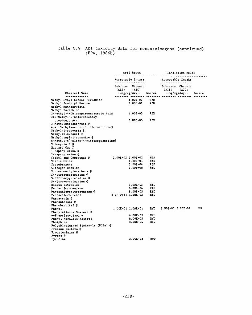
Table C . 4 AD1 toxicity data for noncarcinogens (continued) (EPA, 1986b)
Acceptable Intake
Subchron Chronic (AIS) (AIC)
-----------------
--mg/kg/day-- Source -------- -------- - - - - - - - 8.00E-03 RfD 5.00E-02 RfD
1.OOE-03 RfD
3.OOE-03 RfD
Chemical Same
Yethyl Echyl Ketone Perioxide 3ethyl Isobutyl Ketone Yethyl Methacrylate Yethy1 Parathion 2-!lethyl---Chlorophenoxyacetic Acid 1 (2-?lethyl---Chlorophenoxy)
3-!'lechylcholanthrene @ ; , ~ ' - ? l e t h y l e n e - b i s - ? - c h l o r o a n i l i n e @ Yethylnitrosourea C Yethylthiouracil @' Elethylvinylnirrosamine @ N-Yechyl-N'-nicro-~-nitrosoguanadrnc@ YltOmyCin C @ !lustard Gas C 1-Xapthylamme @ ?-Napthylamine @ Sickel and Compounds @ 2.00E-02 1.00E-02 Sitric Oxide 1.00E-01 Sitrobenzene 5 . OOE-04 Sitrogen Dioxide 1.00E+00 Nitrosome'chylurerhane @ N-Nitrosopiperidine @ S-Sicrosopyrrolidine @ 5-Nitro-o-toluidine @ Osmium Tetroxide 1.OOE-05 Pentachlorobenzrne 8.00E-04 Pentachloronitrobenzene @ 8.00E-03 Pentachlorophenol 3.OE-2(T) 3.00E-02 Phenacetin @ Phcnanchrene @ Phenobarbital @ Pheno 1 Phenylalanine ?lustard @ m-Phenylenediamine Phenyl ?lercuric Acetate Phosphine Polychlorinated Biphenyls (PCBs) @ Propane Suleone @ Propylenimine @ Pyrene @ Pyridine
- - - - - - - - - - - - -
propionic Acid
HEA RfD RfD RfD
RfD RfD RfD RfD
1.00E-01 1'.00E-01 RfD 1.90E-01 2.00E-02 HEA
6.00E-03 RfD 8.00E-05 RfD 3.00E-04 RfD
2.00.E-03 ,RfD
-258-
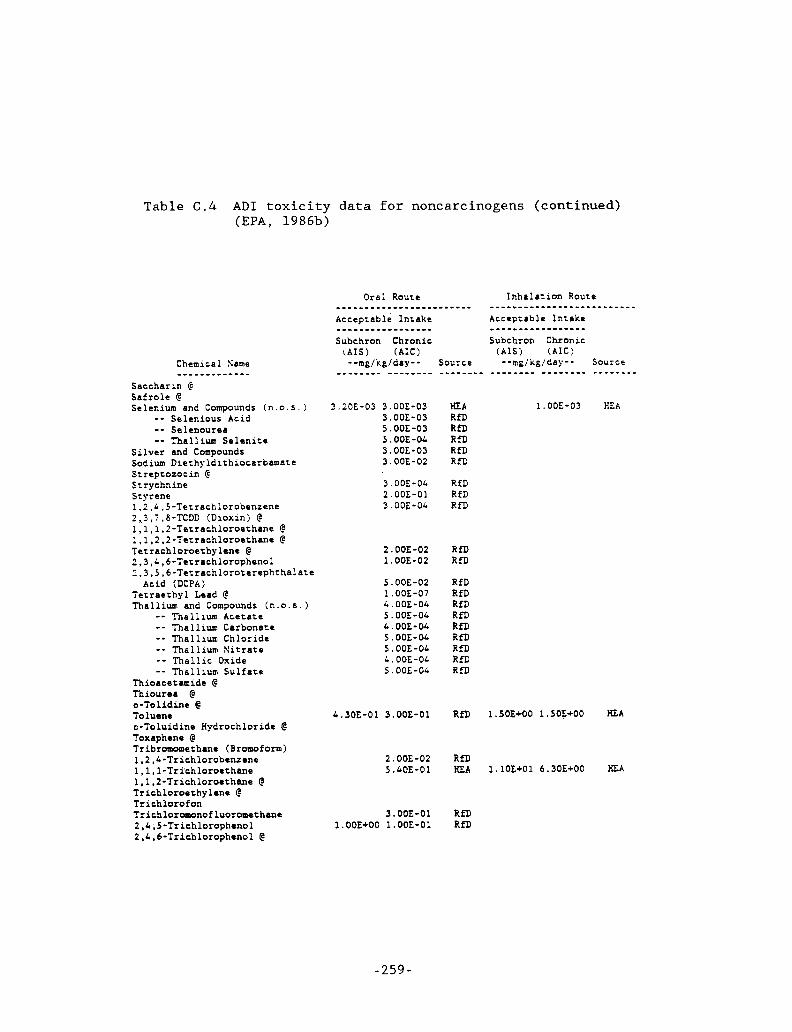
Table C . 4 AD1 toxicity data for noncarcinogens (continued) (EPA, 1986b)
Chemical Same - - - - - - - - - - - - - Saccharin CC Safrole @ Selenium and Compounds (n.o.s.1 - - Selenious Acld -- Selenourea -- Thallium Selenite Silver and Compounds Sodium Diethyldithiocarbamate Streptozocin CC Strychnine Styrene 1.2,L,5-Terrachlorobenzene 2,,3,i,G-TCDD (Dioxin) @ 1,1,1,2-Tetrachloroerhane @ 1.1,2.2-Tezrachloroerhanr @ Tetrachloroethylene @ 2,3,L,6-Tcrrachlorophenol 2,3,5,6-Terrachloroterephtl-4alate
Tetraethyl Lead @ Thallium and Compounds (n.0.s.)
Acid (DCPA)
-- Thallium Acetate -- Thallium Carbonate -- Thallium Chloride - - Thallium Nitrate -- Thallic Oxide - - Thallium Sulfate ThioAcetamide @ Thiourea @ o-Tolidine @ Toluene o-Toluidine Hydrochloride @ Toxaphene @ Tribromomethane (Bromoform) 1.2,L-Trichlorobenzene l,l,l-Trkhloroethane 1,1,2-Trichloroerhane @ Trichloroethylene @ Trichlorofon Trichloromonofluoromethane 2,L.5-Trichlorophanol 2,~,6-Trichlorophenol @
3.20E-03 3.00E-03 3.00E-03 5 . DOE-03 5.OOE-04 3.00E-03 3.OOE-02
3.00E-OL 2.00E-01 3.ODE-OL
2.00E-02 1.OOE-02
5.00E-02 1.006-07 L . OOE-04 5.OOE-OL L . OOE-OL 5.00E-0L 5 . OOE-OL 1,. DOE-OL 5 . OOE-OL
L . 30E-01 3.00E-01
2.00E-02 5 .LOE-Ol
3.00E-01 1.00E+00 1.00E-01
- 2 5 9 -
H E A RfD RED RfD RfD R fD
RfD RfD RfD
RfD RfD
RfD RfD RID RfD RfD RfD RID RfD RfD
RfD
R f D HEA
R f D R f D
1.00E-03
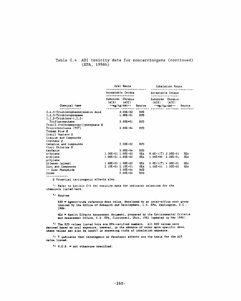
Table C.4 AD1 toxicity data for noncarcinogens (continued) (EPA, 1986b)
Chemical Kame ------I------
?. ,&, .Trichlorophenoxyaca 1,2,3-Trichloropropane 1.1,2-frichloro-1,~,2- Trifluoroethane
LC Acid
Tris(2,3-dibromopropyl)phosphate @ Trinitrotoluene (ThT) ?-an Blue @ Uracil ?lustarc! Q Uranium and Compounds Crethane @ Vanadium and Compounds Vinyl Chloride @ Yarfarin
3.00E-02 1.00E-01
3.OOE+O 1
Z.OOE-O&
2.00E-02
3 . DOE-OL 0- Sy 1 ene 1.00E-01 1.00E-02 m-Sy lene 1.00E-01 1.OOE-02
Zinc and Compounds 2.10E-01 2.lOE-01
p-Xylene Xylenes (mixed) 1.00E-01 1.00E-02
-- Zinc Phosphide 3 . 00E-0& Zineb S.00E-02 - - - - - - - - - - - - -
@ Potential carcinogenic effeczs also.
RfD RfD
RfD
RfD
RfD
R fD HEA 9.6E-I(T) Z.OOE-01 HEA HEA 1.00E+00 2.00E-01 %A
HEA E A RfD RfD
6.9E-l(T) L.OOE-01 KEA 1.00E-01 1.00E-02 KEA
I - Refer to Exhibit C-5 for toxicity data for indicator selection for the chemicals listed here.
*J Sources
RfD = Agency-wide reference dose value, developed by an inter-office work group chaired by the Office of Research and Development, C . S . EPA, Washington, D.C., 1986.
E A = Health Effects Assessment document, prepared by the Environmental Criteria and Assessment Office, U.S. EPA, Cincinnati, Ohio, 1985 (updated in nay 1986).
'J The RfD values listed here are EPA-verified numbers. All RfD values were derived based on oral exposure; however, in the absence of other more specific data. these values may also be useful in assessing risks of inhalation exposure.
'J T indicates chat teratogenic or fatotoxic effects are the basis for the AIS value listed.
'' N . O . S . = not otherwise specified.
- 260-
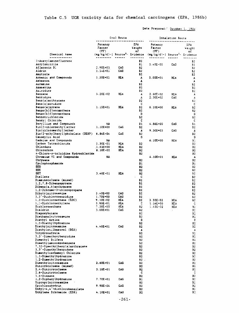
I.
I
.-
Table C . 5 UCR tox ic i ty data f o r chemical carcinogens (EPA, 1986b)
Dare Prepare&:- ~czobcr 1 .XC
Chemical hame
2-Acetylarcinofluorene Acrylonitrile Aflatoxin 81 Aldrin Amitrole Arsenic and Compounds Asbestos Auramine Azaser q e Azir id ine Benzene Benriaine Benz(a)anthracene Benz(c)ocridine Benzo(a)pyrene Benzo(b)fluoranrhene Benzo(k)fluoranthene Benzotrichloride Benzyl Chloride Beryllium And Compounds KA Eis(2-ch1oroethyl)ether l.lOE+OO Bis(chloromethy1)erhcr Eis(2-ethylhexy1)phthalate (DEHP) 6.84E-Ob Cacodylic Acid CAdmiUIn and Compounds NA Carbon Tetrachloride 1.30E-01 Chlordane 1.61E+00 Chloroform 8.10E-02
-------------
b-Chloro-o-toluidine Hydrochloride
CAG
CAG
M A HEA HEA
Chromium VI and Compounds Chrysmne Cyclophosphmide DDD DDE DDT Dial late Diaminotoluene (mixed) 1.2.7,8-Dibenzopyrene Dibcnz(a,h)anthracene 1.2-Dibromo-3-chloropropane Diburylnirrosamine 3,3'-Dichlorobenzidine 1.2-Dichloroethane (EDC) 1,l-Dichloroethylcne Dichloromcthane Dieldrin Diepoxyburane Diethanolnirrosamine Diethyl Arsine 1.2-Diethylhydrazine Diethylnitrosamine Diethylstilbestrol (DES) D ihydros r f ro 1s j,3'-Dimerhoxpbenzidine Dimethyl Sulfate Dimethylaminoarobenzene 7,l~-Dimcthylbenz~a)anrhracene 3,3'-Dime~h~~lbenzidenc Dimerhylcarbamoyl Chloride 1,l-Dimethylhydrazine 1.2-Dimethylhydrazine Dimrthy lnit rosamine Dinitretoluene (mixed) 2,A-Dinitro~oluene 2.6-Dinitrotoluene 1.L-Dioxanc 1.2-Diphenylhydrazine Dipropylnitrosamine Epichlorohydrin Erhyl-b,L'-dichlorobenzilate Ethylene Dibromide (EDB)
Oral Route -_ - - - - -_______- -____________ Potency EPA Factor Keight (PY) of
(mg/kg/d)-l Sourcez- Evidence _ _ _ - - - - - _ _ _ _ _ _ _ _ _ _ _ _ _ - _ B2 B1
2.90E+03 CAG B2 l.liE+Ol CAG B2
B? 1.50E+01 HEA A
A B2 B2 82
A h B2 C
B2 B2 D 82 C
B1 B2 A 82 D
j.?OE-02 H E A
l.ljE+Ol E A
NA
3.LOE-01 HEA
j.iOE+OO CAG 1.70E+00 CAG 9.10E-02 HEA 5.80E-01, HEb 7.jOE-03 HEA 3.00E+01 CAG
L.LOE+Ol CAG
2.60E+01
3.10E-01
7.70E-01
9.90E-OL
L .10E+Ol
CAG
CAG
CAG
CAG
CAG
- 2 6 1 -
B2 B2 B2 B2
B2 B1 B2 B2 B2 C B2 B2 82 B2 82 82 B2
c B2 82 B2 B2 D 82 82 A 82 B2 B2 B2 82 82 B2 B2 B2 B2 BZ B2 C B2 B1 B2 82 BZ B2
- - - - - - - - - 2. UOE-0 1
5.OOE+01
2.60E-02 2.30E+02
6.10E+00
L .86E+OO
9.30E+Oj
6.10E+00
4. lOE+01
3. jOE-02 1.lOE+00 1 .L3E-O2
_ _ _ _ _ - CAG
HEA
HZA CAG
HEA
CAG
CAG
E A
HEA
HEA H E A HEA
- - - - _ _ _ _ E? E1 E? B2 B? A A E2 E? E2
A A
E? C 62 E? D E? C
E1 E2
A B? D
El E? 82 B2 82 A 82 B1 E2 E2 B2 B? B? B? B? B? 82 B? B? C
9' E? 92 B? D B? 32
A E' B2 E2 B2 82 82 B? E2 B2 E2 B2 B? C B2 B? 6: 82 B? 8 2
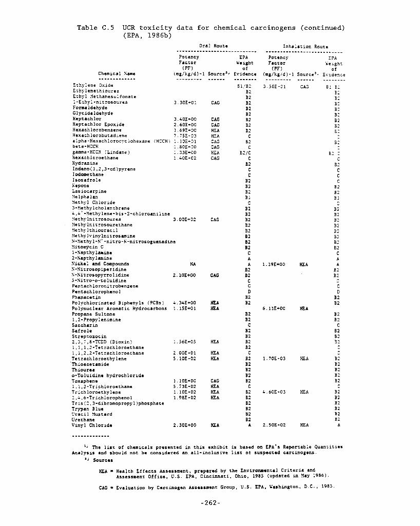
Table C.5 UCR toxicity data for chemical carcinogens (continued)
Ethylene Oxide Ethylenechiourea Ethyl Xethanesulfonate 1-Ethyl-nitrosourea 3.30EIOl Formaldehyde Glycidaldehyde
Heptachlor Epoxide 2.60E+00 Hexachlorobenzene 1.69E100 Hexachlorobutadiene 7.75E-C?3 alpha-Hexachlorocyciohexane (HCCH) l.lOE+Ol beta-HCCH 1.60E100 gamma-HCCH (Lindane) 1.33E+00 Hexachloroechane 1. UOE-02 Hyd rat ine Indeno(l,?,3-cd)pyrene Iodomethane Isosafrole Kepone Las iocarpine Yelphalan Xerhyl Chloride 3-?le~hylcholanthrene I,L'-!lezhylene-bis-?-chloroaniline !lethylnitrosourea 3.00E+02 5e thy lnit rosourerhane !let h y 1 t h i ourac i 1 !lethylvinylnitrosamine N-Methyl-SI-nitro-K-nitrosoguanadine
Heptachlor 3 .LOE+OO
Yitomycin C 1-Napthylamine 2-Saprhylamine Sickel and Compounds S-Nitrosopiperidine S-Sitrosopyrrolidine 5-Nitro-o-toluidine Pentachloronicrobenzene Pentachlorophenol Phenacetin Polychlorinated Biphenyls (PCBs) Polynuclear Aromatic Hydrocarbons Propane Sultone 1.2-Propylenimine Saccharin Safrole Streptotocin 2,3,7,6-TCDD (Dioxin) 1,1,1,2-fecrachloroerhane 1,1,2.2-Tetrachloroechane Tetrachloroethylene Thioacetamide Thiourea o-Toluidine hydrochloride Toxaphene 1.1,2-Trichlorocthane Trichloroethylene 2,-,6-Trichlorophenol Tris(2,3-dibromopropyl)phosphate Trypan Blue Cracil Yustard tirethane Vinyl Chloride
CAG
CAG CAG HEA E A CAG CAG HEA CAG
CAG
NA
2.10E+00 CAG
A. 3LE+00 1 . lX+O 1
KEA HEA
l.56E+O5 HEA
2.00E-01 HEA 5.lOE-02 HEA
l.lOE+OO 5.73E-02 1.1OE-02 1.98E-02
2.30E+00
CAG H E A HEA HEA
Bl,'B? B2 BZ B2 BZ B2 B2 B2 B? C
B2 C
B?/C C
B2 C C
B2 B2 B2 Bl C B2 BZ BZ 82 B2 82 B2 B2 C A A
BZ B2 C C D BZ B2
B2 82 C B2 B2 B? B2 C B2 82 B2 BZ 82 C BZ 82 82 82 B2 B2 A
- - - - - - - - - 3.50E -0 1
1.19E+00
6.11E+00
1.70E-03
L . 60E-03
2.50E-02
- - - - - - - - - - _ _ - - CAG E: E:
€ 2 E: 62 B? E: B2 E' E:
E:
E2 'C C
B' C C C
B? B? E:
C 62 B2 E? E? E: B2 B? B2 C A
HEA A B? B?
C D B2 BZ
B2 82 C B2 B? E2
C C
M A B2 B? B? B? E2 C
M A B2 BZ E? B2 B2 E2
HEA A
HEA
I' The list of chemicals presented in this exhibit is based on EPA's Reportable Quantities
* J Sources Analysis and should not be considered an.al1-inclusive list or suspected carcinogens.
HEA Health Effects Assessment, prepared by the Environmental Criteria and Assessment Office, U . S . EPA, Cincinnati, Ohio, 1985 (updated in !lay 1986).
CAG = Evaluation by Carcinogen Arrestment Group, U . S . EPA, L'Ashington. D.C., 1985.
-262 -
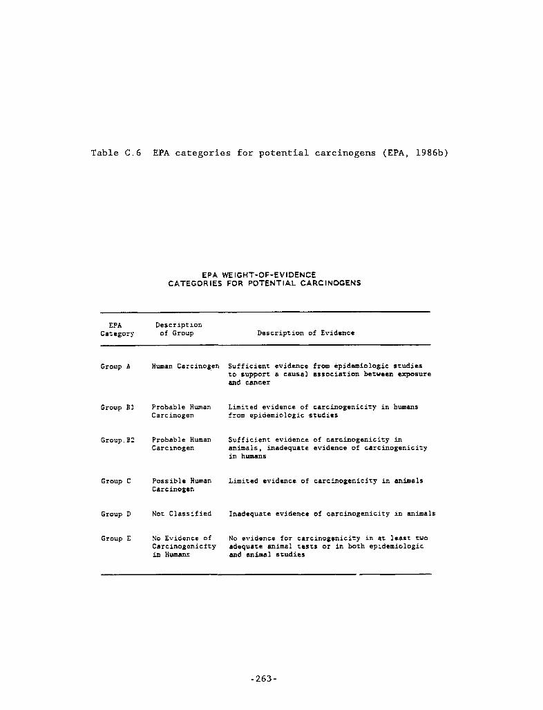
Table C . 6 EPA categories f o r po ten t ia l carcinogens (EPA, 1986b)
EPA WEIGHT-OF-EVIDENCE CATEGORIES FOR POTENTIAL CARCINOGENS
EPA Description Category of Group Description of Evidence
.- . Group A Human Carcinogen Sufficient evidence from epidemiologic studies
to support a causal association betveen exposure and cancer
Group BI Probable Human Limited evidence of carcinogenicity in humans Carcinogen from epidemiologic studies
Group. B?. Probable Human Sufficient evidence of carcinogenicity in Carcinogen animals, inadequate evidence of carcinogenicity
in humans
Group C Possible Human Limited evidence of carcinogenicity in animals Carcinogen
Group D Not Classified Inadequate evidence of carcinogenicity in animals
Group E No Evidence of No evidence for carcinogenicity in a t least two Carcinogenicity adequate animal tests or in both epidemiologic in Humans and animal studies
- -263-
. . - . . . - - -.- --x .- -"- .- " . . .
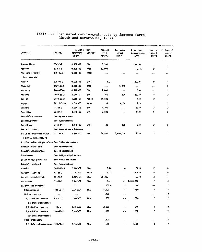
Table C . 7 Estimated carcinogenic potency factors (CPFs) (Smith and Barnthouse, 1987)
Chemical Health ef fects Aquatic I r r i ga ted Fish bio- Health Ecological
CAS No. Benchmark Sourcea l i f e crops a c c w l a t i m hazard hazard (Irg/d) ( W L ) (ll9/L) W k g ) score score
Acenaph thene
Acetone
Aldicarb [Temit]
[ Carban01 a t e l
A ldr in
Aluninun
Antimony
Arsenic
Bariun
Baygon
Benzene
Benzi d i ne
Benzo(a)anthracene
Benzo (a) pyrene
Beryl 1 iun
BnC and Isomers
Bis(2-chloroethyl) ether
[ d i chloroethylether 1 Bis(2-ethylhexyl) phthalate
Branochlomthane
B d i c h l o r c r n e t h a n e
2-Butanone
Butyl benzyl phthalate
2-Butyl l-octaool
Cadniun
Carbaryl [Sevinl
Carbon tetrachloride
Chlordane
Chlorinated benzenes
Chlorobenzene
Dichlorobenzene
1,2-Oichlorobenzene
I 0-d i ch 1 orabenzene I 1.3-0ichloroknzene
1,4-Oichloroknzene
[p-dichlombenzenel
Trichlorobenzene
1,2.4-Trichlorobenzene
83-32-9
61-64-1
116-06-3
309-00-2
1429 -90-5
1440-36-0
1440-38-2
1440-39-3
381 11-13-8
11-43-2
92-81-5
O.aoE42
0.40E42
0.66E-02
0.W-06
3.oa*Oo
0.29243
O.O4E+W
1.m-01
0.12E+Oo
0.3OE42
0. ME-02
See Hydrocarbons
See Hydrocarttons
1440-41-7 0.17Em
See Hexachlorocyclohexane
111-44-4 0.84€+00
See Phthalate esters
see HaloTethanes
see Halolnethanes
See Methyl e thy l ketone
See Phthalate esters
See Hydrocarbons
1440-43-9 0.2E42
63-25-2 0.18E41
56-23-5 0.52E*01
51-14-9 0.24E-02 _- --
108-90-7 0 . 2 6 6 4
-- -- 95-50-1 0.46E43
None 0.46E43
106-46-7 0.46E43
__ -- 120-82-1 0.14E42
EPA
wsn wsn
EPA
wsn EPA
EPA
m a n wsn EPA
EPA
EPA
EPA
EPA
wsn EPA
€PA
EPA
€PA
EPA
EPA
EPA
1.700
10,Ooo
--
3.0 --
9,Ooo 360
14.500
13
5.300
2,500
130
54,400
0.66
1.7
35,200
2.4
250.0
15.900
1,120
1.580
2.850
1.120
1,500
1.500
390.0
0.16
--
11.Ooo.o
-- 1 .o
280.0
4.0
8.5
32.0
41 .O
2.0
11.0
10 50.0
-- 200.0
__ 23.0
-- 1,400,Ooo
-- -- _ _ 450
-- 560
._ 140
-- 690
3
2 --
9
-- _ _ 4
2
2
2
5
2
3
2
2
2
1
_ _
4
2
2
2
1
2
2
2
2
1
2
2
2
2
-264-
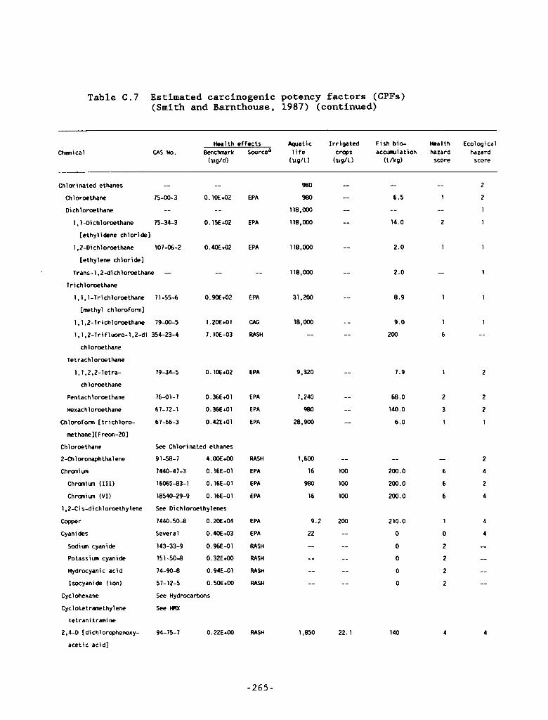
Table C.7 Estimated carcinogenic potency factors (CPFs) (Smith and Barnthouse, 1987) (continued)
Health effects Aquatic Irrigated Fish bio- Health Ecological CAS No. Benctmurlt Sourcea life crops accwlation hazard hazard
(vg/d) ( l lg /L) ( l lg /L) (L/C9) score score Chemical
Chlorinated ethanes -- Chloroethane 75-00-3 Oichloroethane _- 1.1-Oichloroethane 75-34-3
[ethylidene chloride]
1 ,Z-Dichloroethane 107-06-2
[ethylene chloride]
Trans-1 ,Z-dichloroethane --
2
2
1
1
1
1
1
1 _ _
_-
0.1of42 -_
0 .15E42
0.40E42
_-
0.9oE+02
1.2DE+o1
7.W-03
O.loE42
0.36E41
0.36E41
0.42E41
-- 6 . 5
-- 14.0
2.0
2.0
8.9
9.0
200
€PA
€PA
€PA
--
EPA
CAC
RASH
€PA
EPA
EPA
€PA
RASH
€PA
EPA
€PA
€PA
€PA
RASH
RASH
RASH
RASH
RASH
118,Ooo -- I-
118.Ooo -- Trichloroethane
1.1.1-Trichloroethane
[methyl ch 1 oroform]
l,l,Z-Trichloroethane
1,1.2-Trifluoro-l .2-di
chloroethane
Tetrachloroethane
1.1.2.2-Tetra-
chloroethane
Pentachl orwthane
Hexachloroethane
Chloroform [trichloro-
methane 1 [ Freon-201 Chloroethane
2-Chloronaphthalene
Chraniun
Chraniun (111)
Chraniun ( V I )
1.2-Ci s-di chloroethyl ene
Copper Cyanides
Sodiun cyanide
Potassiun cyanide
Hydrocyanic acid
Isocyanide (ion)
Cyclohexane
Cyclotetramethylene
tetrani traine
2,4-0 [ di chl orophenoxy-
acetic acid]
71-55-6
79-00-5
354-23-4
79-34-5
76-01-7
67-72-1
67-66-3
31,200 --
7.9 1 2 9,320
-- 7, 240
980
28,900
68.0
140.0
6.0
See Chlorinated ethanes
91-58-7 4.ooE+00
7440-47-3 0.16E-01
16065-83-1 0.16E-01
18540-29-9 0.16E-01
See Di chl oroe t hy 1 enes
7440-50-8 0.2OE+o4
Several 0.4OE43
143-33-9 O.%E-01
151-50-8 0.32€+00
74-90-8 0.94E-01
57-12-5 0.50€+00
See Hydrocarbons
see My
1.600 -- 16 100
980 100
16 100
_- -- 200.0 6
200.0 6
200.0 6
210.0 1
0 0
0 2
0 2
0 2
0 2
4
4
I
1.850 22.1 140 4 4 94- 75- 7 0.22€+00
-265-
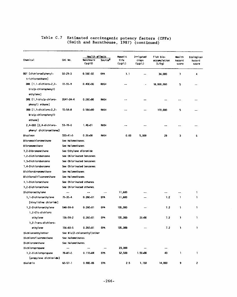
Table C.7 Estimated carcinogenic potency factors (CPFs) (Smith and Barnthouse, 1987) (continued)
Chemical Health effects Aquatic Irrigated Fish bio- Health Ecological
CAS No. Benchrk Sourcea life crops accwlation hazard hazard (llgld) ( l lg /L) ( l l 9 I L ) (Llkg) score score
COT [ di chlorodiphenyl-
trichlomethane]
DDE [l,l-dichloro-2,2-
bis(p-chlorophenyl)
ethylene]
WE [I. l-bis(p-chloro- phenyl) ethane1
OOO [l.l-dichloro-2.2-
bi s (p-chlorophenyl)
ethane]
2.4-000 [2,4-di chloro-
phen y 1 di ch 1 oroethane 1 Diazinon
Oi bmmKhlomthane
Oi brcmDmethane
1 .Z-Dibr-thane
1.2-Oichlorobenzene
1.3-Dichlorobenzene
1.4-Oichlorobenzene
Oichlorobr-thane
Dichlorodi f luoranethane
1.1-Oichloroethane
1 ,2-Oi chlomethane
Oichloroethylene
1,LOichloroethylene
[Vinylidine chloride]
1.2-Oichlomethylene
1 ,Z-Cis-dichloru
ethylene
1 .2-Trans-dichloro-
e thy 1 ene
Oichlorcethylether
Oi ch lorof 1 uoranethane
Dichlomthane
Dichloropropane
1.2-Dichloropropane
[propylene dichloride]
Dieldrin
50-29-3 0.56E-02
72-55-9 0.4OEcoO
3541-04-4 0.26EcoO
72-54-8 0.56ElOO
53-19-0 1.4E41
333-4 1-5 0.2€+00
See Halanethanes
See Halanethanes
See Ethylene dibronide
See Chlorinated benzenes
7 4 34,000 EPA 1.1 --
wsn -- - - 18.000.Ooo 5 _-
RAsn
RASH
RASH
RASH
-- --
0.03 5,000
See Chlorinated benzenes
See Chlorinated benzenes
see Halanethanes
See Halanethanes
See Chlorinated ethanes
See Chlorinated ethanes -- --
75-35-4 0.26E41
540-59-0 0.26E41
156-59-2 0.26EA 1
156-60-5 0.26E41
_- €PA
EPA
EPA
EPA
See Bis(2-chloroethyl)ether
See Halanethanes
See Halanethanes - - --
78-87-5 O.llE44 EPA
60-57 -1 0.9E-06 EPA
11,600 L-
11.600 -
135.000 _-
135.000 2E&
135,000 --
7.2 1
7.2 1
7.2 1
23,000 -- -- 52,500 1.5Ed 43
2 . 5 1.150 14.000
1
1
1
-266-
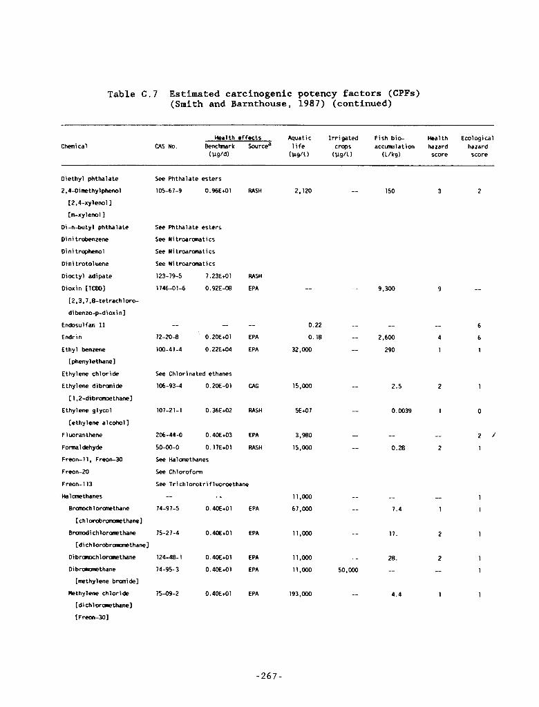
Table C.7 Estimated carcinogenic potency factors (CPFs) (Smith and Barnthouse, 1987) (continued)
Health effects Aquatic Irrigated Fish bio- Health Ecological CAS No. Benchnark Source' life crops accunulation hazard hazard
(vgld) (ll9IL) (ll9IL) (LIk9) score score Chemical
Oiethyl phthalate
2,4-Oirnethylphenol
[2.4-xylenol I [m-xylenol 1
Oi-n-butyl phthalale
Din i trobenzene
Oini trophenol
Dini trotolwne
Oioctyl adipate
Dioxin [TCCO]
[2.3.7.8-tetrachloro-
di benzo-p-diox i n]
Endosulfan I1
Endrin
Ethyl benzene
[phenylethanel
Ethylene chloride
Ethylene dibranide
[ 1.2-dibramethanel
Ethylene glycol
[ethylene alcohol I F 1 ucranthene
Formaldehyde
Freon-1 1, Freon-30
Freon-20
Freon-113
Hal anethanes
Branchloranethane
[chlorobmna~thanel
Brmpdi chl oranethane
See Phthalate esters
105-67-9 O.%E+01 RASH 2,120 _ _ 150 3 2
See Phthalate esters
See Ni troaranatics
See Nitroaranatics
See Nitroarmtics
123-79-5 1.23E+01
1746-0 1-6 0.92E-08
RASH
EPA __ 9,300 9
_-
4
1
-- 0.22 -_ -- EPA 0.18 -- 2.600
EPA 32.000 __ 290
-- _- 72-20-8 ' 0.20€+01
100-41-4 0.22E+04
See Chlorinated ethanes
106-93-4 0.2oE-01 15.000 _ _ 2.5 2 1 CAC
107-21-1 0.36E+02 RASH 5E+07 -_ 0.0039 1 0
--
I
2M-44-0 0.4OE+03
50-00-0 0.17E+01
See Halanethanes
See Chloroform
EPA
RASH
3.980
15.000
See Tr i chlorotr i f 1 uoroethane
__ -- 11,000
74-97-5 0.40E+01 EPA 67,000
I-
- 15-2 7-4 0.4OE+01 EPA 11,000 17. 2 1 -_ Id i ch 1 orobranane thane]
Di branochlomnethane 124-48- 1 0.4OE+01 EPA 11,Ooo
Dibr-thane 74-95-3 0.4OE41 EPA 1 1 ,000
[methylene branide]
Methylene chloride 75-09-2 0.40E+01 EPA 193,000
[dichloranethanel
[ F reon-301
_ _ 28. 2 1
1 50,000 __ __
4.4 1 1 _ _
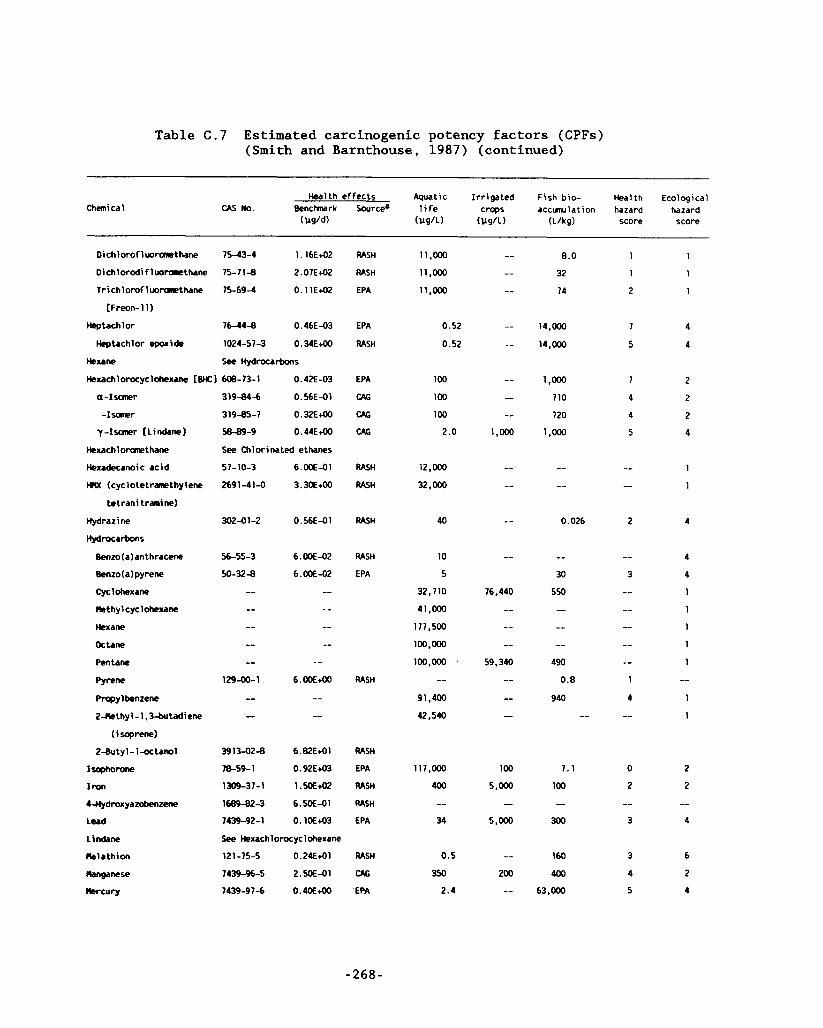
Table C.7 Estimated carcinogenic potency factors (CPFs) (Smith and Barnthouse, 1987) (continued)
Chemical Health ef fects Aquatic I r r i ga ted Fish bic- Health Ecological
CAS No. B e n c h r k Sourcea l i f e crops accunulation hazard hazard (vg ld) (vg/L) (vg/ t ) (Llkg) score score
O i c h l o r o f l w m t h a n e 75-43-4 1.16E42
Oichlorodi f 1 uomRthane 75-7 1-8 2.07E+02
T r i c h l o r o F l w m t h a n e 75-69-4 0.11E42
[Freon-1 1)
Heptachlor 16-444 0.46E-03
Heptachlor epoxide 1024-57-3 0.34E+W
Hexane See Hydrocarbons
Hexachlorocyclohexane [BHC] 608-73-1 0.42E-03
a-Isaner
-1saner
y-Isamer [Lindane]
Hexachloramethane
Hexadecanoic ac id
Mx (cyclotetrawthylene
te t ran i tranine)
Hydrazine
Hydrocarbons
Benzo (a) an thracene
Ben20 (a)pyrene
cyclohexane
Methylcyclohexane
Hexane
octane
Pentane
Pyrene
Propylbenzene
2-Methyl-l.3-butadiene
(isoprene)
2-&Jty l - 1- tam1
rsaphorone
I K U l
4Hydroxyazobenzene
Lead
Lindane
Nablathion
*nganese
k r c u r y
319-84-6 0.56E-01
319-85-7 0.32E+W
5889-9 0.44€+00
See Chlorinated ethanes
5 7- 10-3
2691-41-0
302-01-2
56-55-3
50-324 -- -- -- - -
129-00-1
-- -
3913-02-8
78-59-1
1309-37-1
1689-82-3
7439-92-1
6.OOE-01
3.3oE+00
0.56E-01
6.OOE-02
6.OOE-02
_- -- -- --
-- 6.OOE+W
__ --
6.82E4 1
0.92E+03
l . w E 4 2
6.5OE-01
0. WE43
See Hexachlorocyclohexane
12 1-75-5 0.24E4-01
7139-96-5 2.wE-01
7439-97-6 0.4c€+CKl
RASH
RASH
EPA
EPA
RASH
EPA
CAG
CAG
CAG
RASH
RASH
RASH
RASH
EPA
RASH
RASH
EPA
RASH
RASH
EPA
RASH
CAG EPA
11,000
11,000
11,000
0.52
0.52
100
100
100
2.0
12,000
32,000
40
10
5
32.710
41 ,000
177,500
100.000
100,000 ' --
91.400
42,540
117.000
400
-- 34
0.5
350
2.4
8.0
32
14
14,000
14,000
1 ,000
710
120
1 .m
-- --
0.026
-- 30
550
_- -- --
490
0.8
940
--
7.1
100
-- 300
160
400
63.000
1
1
1
4
4
2
2
2
4
1
1
4
4
4
1
1
1
1
1
__ 1
1
2
2
-- 4
6
2
4
-268-
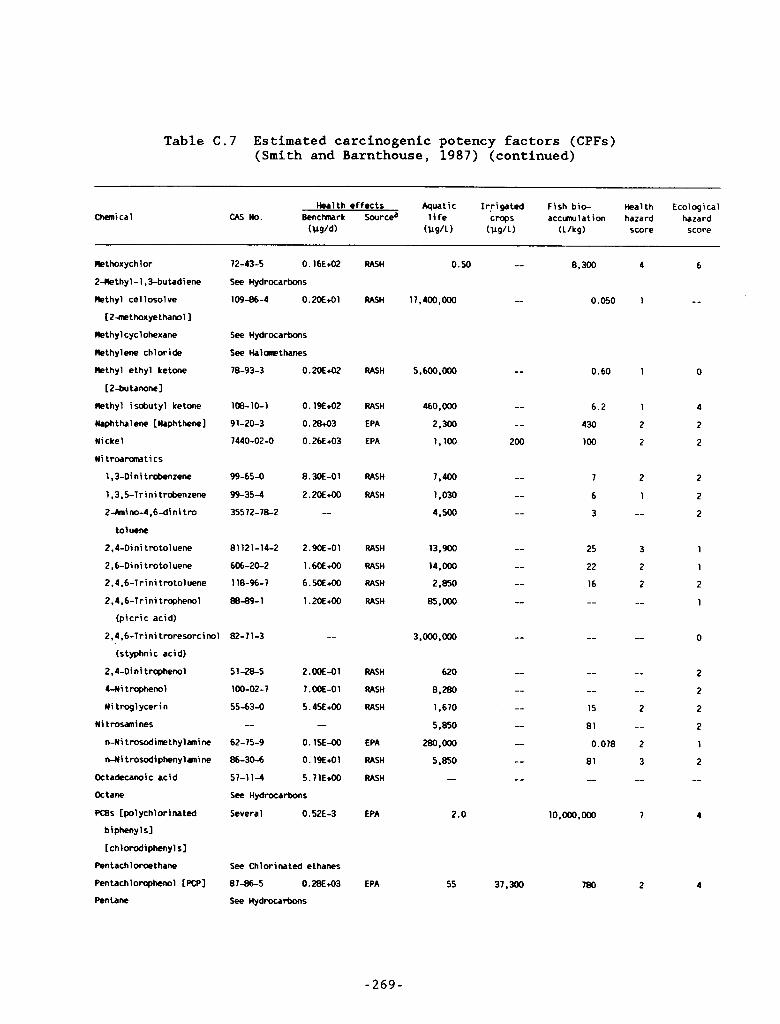
I
I-
-
Table C . 7 Estimated carcinogenic potency factors (CPFs) (Smith and Barnthouse, 1987) (continued)
Chernical Health effects Aquatic Irrigated Fish bio- Health Ecological
CAS No. Benchark Sourcea life crops accunulation hazard hazard ( W d ) ( W L ) (llg/L) (Llkg) score score
Methoxych 1 or
2-Methyl-1.3-bu tadiene
Methyl cellosolve
[2+mthoxyethanol]
Methylcyclohexane
Methylene chloride
Methyl ethyl ketone
[2-butanonel
nethyl isobutyl ketone
Naph t ha1 ene [Naph thene 1 Nickel
Ni troamti cs
1.3-Dini trobenzene
1,3,5-Trinitr&enzene
2 A i no-4 ,b-di ni tro
toluene
2.4-Oi ni tro to1 uene
2,b-Oini trotolwne
2.4.6-Trinitrotoluene
2.4.6-Tr i ni trophenol
(picric acid)
2.4,b-Tri ni troresorci no1
(styphnic acid)
2.44 ni trophenol
4-Ni trophenol
Ni trogl ycer i n
Ni trosanines
n-Ni trosodinethylanine
n-Ni trosodi phenyl ani ne
Octadecanoic acid
Octane
PCBs [polychlorinated
biphenyl 51
[chlorodiphenyl SI Pentachloroethane
Pentachlorophenol [PCP]
Pentane
72-43-5 0.1bE4.02
See Hydrocarbons
1094b-4 0.2oE+Ol
See Hydrocarbons
see Halonethanes 18-93-3
108-10-1
91-20-3
1440-02-0
99-65-0
99-35-4
35512-18-2
81121-14-2
bob-20-2
118-96-7
m a - 1
82-71-3
51-28-5
100-02-7
55-63-0 --
b2-75-9
86-30-6
57-11-4
0.2oE+02
0.19E42
0.2843
0.26E+03
8.3oE-01
2 . 2 o E m
--
2.w-01
1.6oEdx)
b.5oEcOO
1.2oEm
--
2.ooE-01
l.ooE-01
5.45Em
-- 0.15E-00
0.19E+01
5.11E40
See Hydrocarbons
Several 0.52E-3
See Chlorinated ethanes
87-86-5 0.28E4.03
See Hydrocarbons
RASH
RASH
RASH
RASH
EPA
EPA
RASH
RASH
RASH
RASH
RASH
RASH
RASH
RASH
RASH
EPA
RASH
RASH
EPA
EPA
0.50
11.400, 000
-- 8.300 4 6
-- 0.050 1 --
5,600,000
4b0.000
2.300
1,100
7,400
1,030
4.500
13.900
14.000
2.850
85.000
3,000.000
620
8,280
1.670
5,850
280,000
5,850
-
2.0
55 37.300
0.bO 1
b.2 1
430 2
100 2
7 2
6 1 3 --
25 3
22 2
2 16
10.000.000 1
0
0
4
780 2 4
- 2 6 9 -
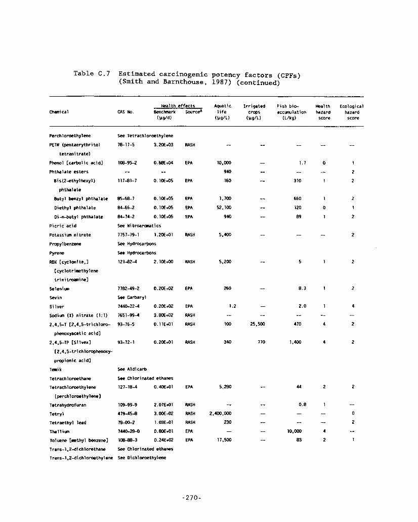
Table C.7 Estimated carcinogenic potency factors (CPFs) (Smith and Barnthouse, 1987) (continued)
Chemical Health effects Aquatic Irrigated Fish bio- Health Ecological
CAS No. Benchark SwrcP life craps accunulation hazard hazard ( W d ) ( W L ) (lAg/1) (Llkg) score score
Perchloroethylene
PETN (pentaerythri to1
tetrani trate)
Pknol [carbolic acid]
Phthalate esters
Bi s (Z-ethyl hexyl)
phthalate
Butyl benzyl phthalate
Diethyl phthalate
Oi-n-butyl phthalate
Picric acid
Potassiun nitrate
Propylbenzene
Pyrene
ROX Icyclmite.1
[ cyclotr imethylene
trini t-inel
Seleniun
Sevin
Silver
Sodim (I) nitrate (1:l)
2,4.5-T [2.4,5-trichloro-
phenoxyacet ic acid]
2.4.5-TP [ S i lvexl
[ 2.4.5-tr i chl orophenoxy- prapimic acidl
Temi k
let rachl oroe thane
Tetrachloroethylene
[perchloroethylene]
Tetrahydrofuran
Tetryl
Tetraethyl lead
Thallium
Toluene [methyl benzene1
Trans-1,2-dichlorethane
See Tetrachloroethylene
78- 17-5 3.2oE43
108-95-2 0.68Ec04 -- -
117-81-7 0.14+05
85-68-7 0.1445
84-66-2 0.1OE45
84-14-2 O.lOE&
See Ni tmranatics
7757-79-1 1.2OE+O1
See Hydrocarbons
See Hydrocarbons
121-82-4 Z.lOE+W
7782-49-2 O.ME42
See Carbaryl
7440-22-4 0.20E42
7651-99-4 3.8OE42
93-76-5 0.11Etol
93-72-1 0.2441
See Aldicarb
See Chlorinated ethanes
127-18-4 0.9OE*ol
109-99-9 2.07E41
479-45-8 3.OOE-02
78-00-2 1.03E-01
7440-28-0 O.BDE41
108-88-3 0.24E42
See Chlorinated ethanes
RASH
€PA
€PA
€PA
€PA
€PA
RASH
RASH
€PA
€PA
RASH
RASH
RASH
€PA
RASH
RASH
RASH
€PA
€PA
I
10,ooo
940
160
1,700
52,100
940
5.400
5,200
260
1.2 -- 100
340
5,280
-- 2.m.ooo
230 -
17,500
--
1.1 -- 310
660
120
89
-
5
8.3
2.0 -- 470
1,400
0 1
-- 2
1 2
1 2
0 1
1 2
1 2
1
1
-- 4
4
44 2
2
2
2
Trans-1 ,Z-dichloroethylene See Oichloroethylene
-270-
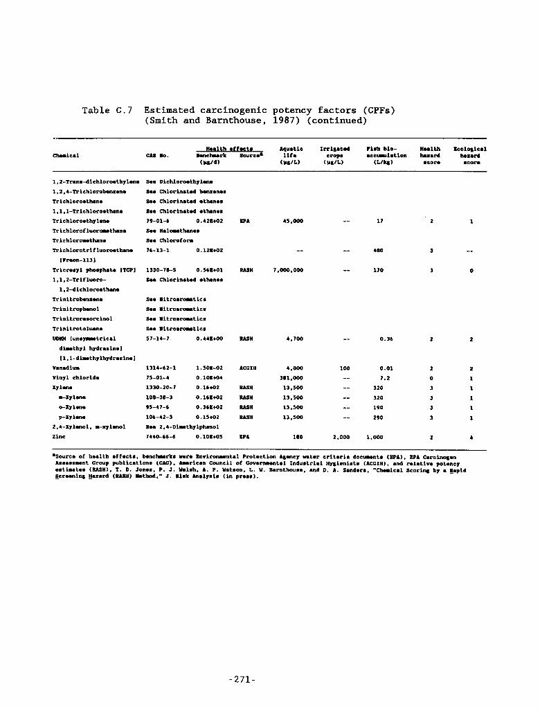
Table C.7 Estimated carcinogenic potency factors (CPFs) (Smith and Barnthouse, 1987) (continued)
Chrle.1
1,2-Trann-dlchloroothylena l,2,4-Trlchlorobanrana Trichloroathma 1.1.1-Trlehloroathma Triehloroathylena Trichlorofluorathana Trichlororthana Trichlorotrifluo~thana
llraon-1131 Trieramyl phosphate ITCPI 1.1.2-TrIFluoro- 1.2-dlchloroathun
Trinltrobanrana Trlnltrophenol Trinltronmorelnol Trlnltrotoluana UDlM lunalutrlcal dluthyl hydrazinal (1.1-dlrthylhydrarln.1
Vanadium Vinyl chloride Iylana *xylan. o-xylm.
p-Xylan* 2.4-XYl~01, D - ~ l ~ O l
Zinc
Sa. 01chloroothyl.na Sa. Chlorinated bmranam Sea Chlorinated *thanes Sam Chlorlruted athanaa 79-01-6 0.4ZtM2
Sea Ihlathanaa Sa. Chloroforr 76-13-1 0.121+02
1330-78-5 0.56EMl Sam Chlorinated athanam
Sa. iitroaratlcm Sam iitroaroutlcm Sam iltroaroutlem Sa* litroaroutlea 57-14-7 0.44EtOO
1314-62-1 1.5OE-02 75-01-4 0.101M4 1330-20-7 0.16M2 108-38-3 0.16EM2 95-47-6 0.36KM2 106-42-3 0.15+02 Sa* 2.4-Dluthylphenol 7440-66-6 0.101+05
I P A
RASH
RASH
ACCIH
BASH
RASH
RASH
RASH
BPA
45.000
--
7,000,000
4,700
4.800
381.000 13.500 13,500 13,500 13.500
180
-- 17
-- 0.36
100 0.01 -- 7.2 -- 320 -- 320
-- 190 -- 290
2,000 1.000
2 1
*Sourea of health affacts. bmeh.rka umra BnVl~onMnt*l Protaction Agancy mtar criteria docuuntm (BPA). EPA Carclnogan Aasamaunt Croup publlcatlona (W). AmriCan Council of Covarnnntal Induatrlal Hyglenista (ACCIH). and relativa potancy amtlutaa (RASH). T. D. Jonam. P. J. Yalmh, A. P. Yataon. I.. Y. Barnthouaa, and D. A. Sanders. "Chenlcal Scoriry by a Eapia &xaenlng Wzard (RASH) Umthod," J. Risk halyalm (in pramm).
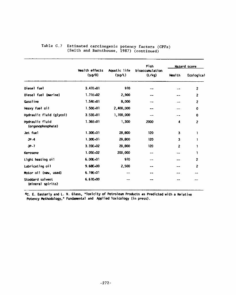
Table C.7 Estimated carcinogenic potency factors (CPFs) (Smith and Barnthouse, 1987) (continued)
Fish Hazard score Health effects Aquatic l i f e b ioaccwla t ion
2 Diesel fuel 3.47E+Ol 970 -- -- Diesel fuel (marine)
Gas01 i ne
Heavy fuel o i l
Hydraulic f l u i d (glycol)
Hydraulic f l u i d (organophosphate)
Jet fuel
JP-4
JP-7
Kerosene
l i g h t heating o i l
Lubricating o i l
Rotor o i l (new, used)
Stoddard solvent (mineral sp i r i ts )
1.3OE+O1
1.3oE+o1
3.33E+O2
1 .05E+02
6.OOE+01
9.68E+OO
6.19E41
120
120
120
3
3
2
--
1
1
1
1
2
2
--
-- %. E. Easterly and 1. R. Glass, “Toxicity Of Petrolem Products as Predicted with a Relative Potency Rethodology,” Fundaental and Agpl ied Toxicology ( i n press).
-272-
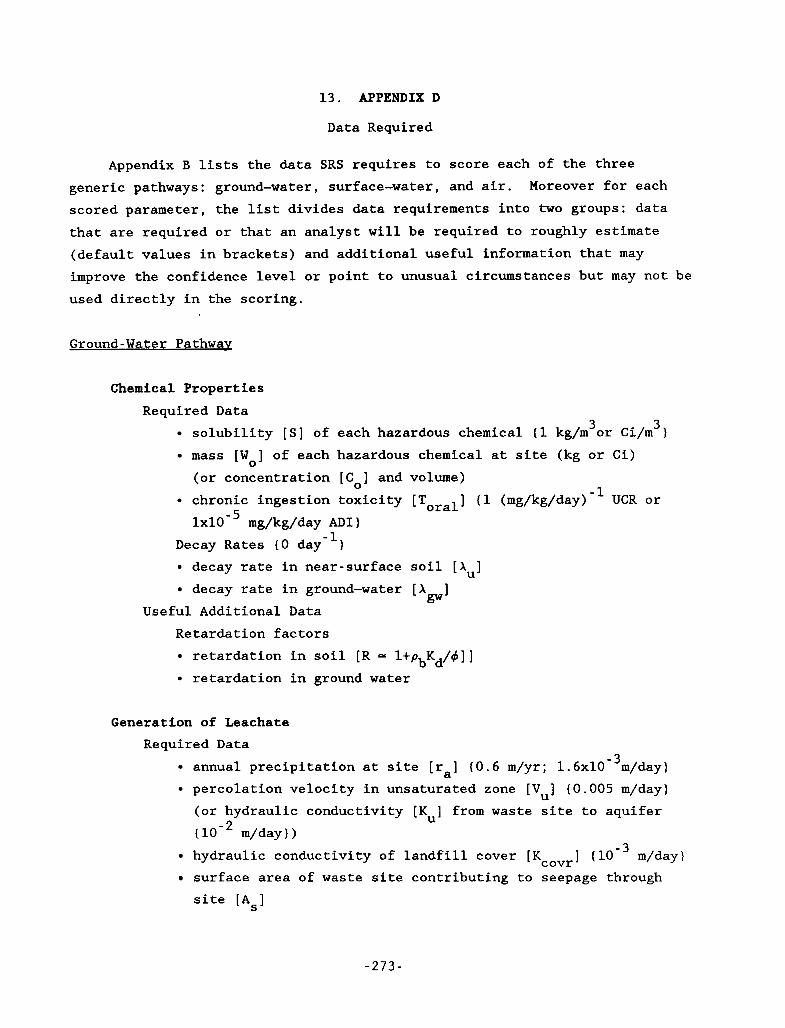
13. APPENDIX D
Data Required
Appendix B lists the data SRS requires to score each of the three generic pathways: ground-water, surface-water, and air. Moreover for each scored parameter, the list divides data requirements into two groups: data that are required or that an analyst will be required to roughly estimate (default values in brackets) and additional useful information that may improve the confidence level or point to unusual circumstances but may not be used directly in the scoring.
Ground-Water Pathway
Chemical Properties
Required Data 3 3 solubility [SI of each hazardous chemical (1 kg/m or Ci/m )
mass [W ] of each hazardous chemical at site (kg or Ci) 0
(or concentration [C ] and volume)
l ~ l O - ~ mg/kg/day AD1 I
0
chronic ingestion toxicity [T
Decay Rates (0 day-') decay rate in near-surface soil [Xu] decay rate in ground-water [ A ]
] (1 (mg/kg/day)-l UCR or oral
gw Useful Additional Data
Retardation factors retardation in soil [R = l + p K /d]] retardation in ground water
b d
Generation of Leachate Required Data
annual precipitation at site [ra] (0.6 m/yr; 1.6~10-~m/day) percolation velocity in unsaturated zone [V ] (0.005 m/dayl
U (or hydraulic conductivity [K ] from waste site to aquifer ( m/day) )
U
hydraulic conductivity of landfill cover [Kcovr] surface area of waste site contributing to seepage through
site [As]
m/dayl
-273-
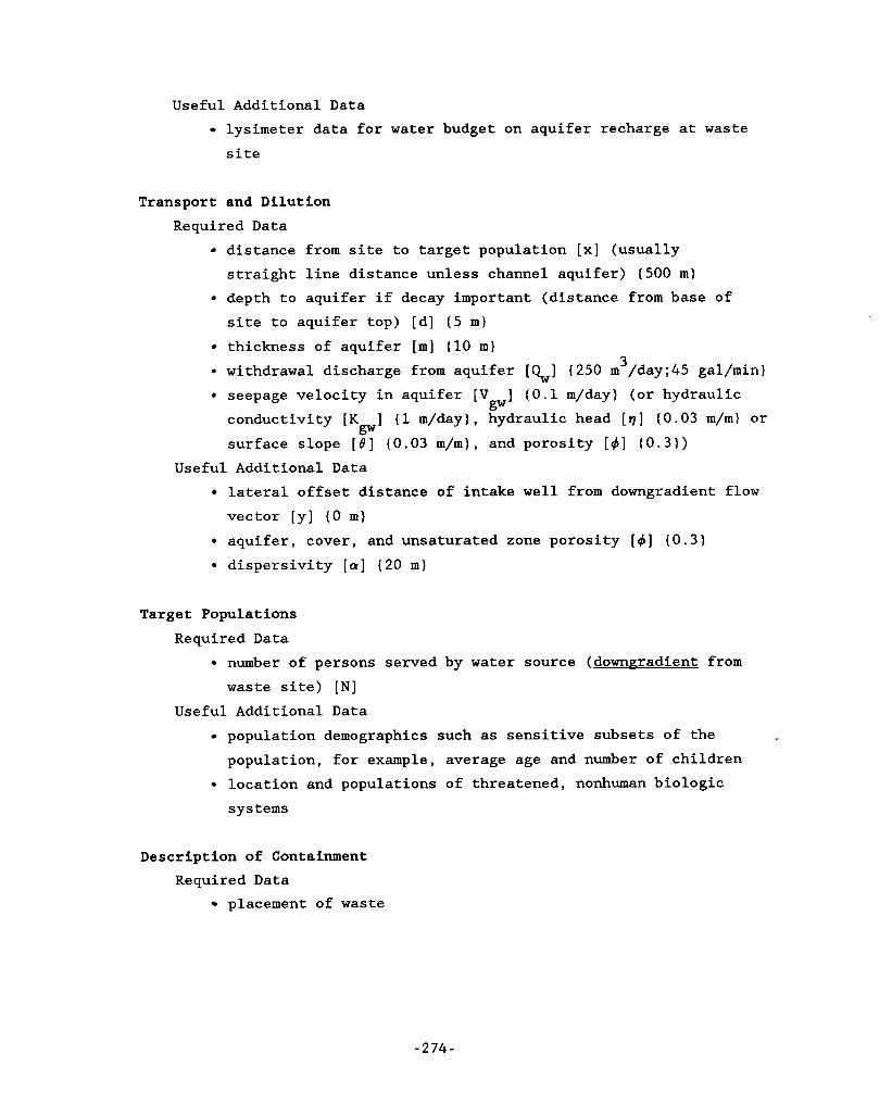
Useful Additional Data lysimeter data for water budget on aquifer recharge at waste
site
Transport and Dilution Required Data
distance from site to target population [XI (usually straight line distance unless channel aquifer) (500 m) depth to aquifer if decay important (distance from base of site to aquifer top) [d] ( 5 m) thickness of aquifer [m] (10 m) withdrawal discharge from aquifer [QJ ( 2 5 0 m /day;45 gal/min) seepage velocity in aquifer [V ] (0.1 m/day) (or hydraulic
3
gw conductivity [K ] (1 m/day), hydraulic head [ q ] (0.03 m/m) or surface slope [e] (0.03 m/m), and porosity [ 4 ] (0.3))
gw
Useful Additional Data lateral offset distance of intake well from downgradient flow vector [y] (0 m) aquifer, cover, and unsaturated zone porosity [ 4 ] (0.3) dispersivity [a] ( 2 0 m)
Target Populations Required Data
number of persons served by water source (downgradient - from waste site) [N]
Useful Additional Data population demographics such as sensitive subsets of the
population, for example, average age and number of children location and populations of threatened, nonhuman biologic systems
Description of Containment Required Data
placement of waste
-274 -
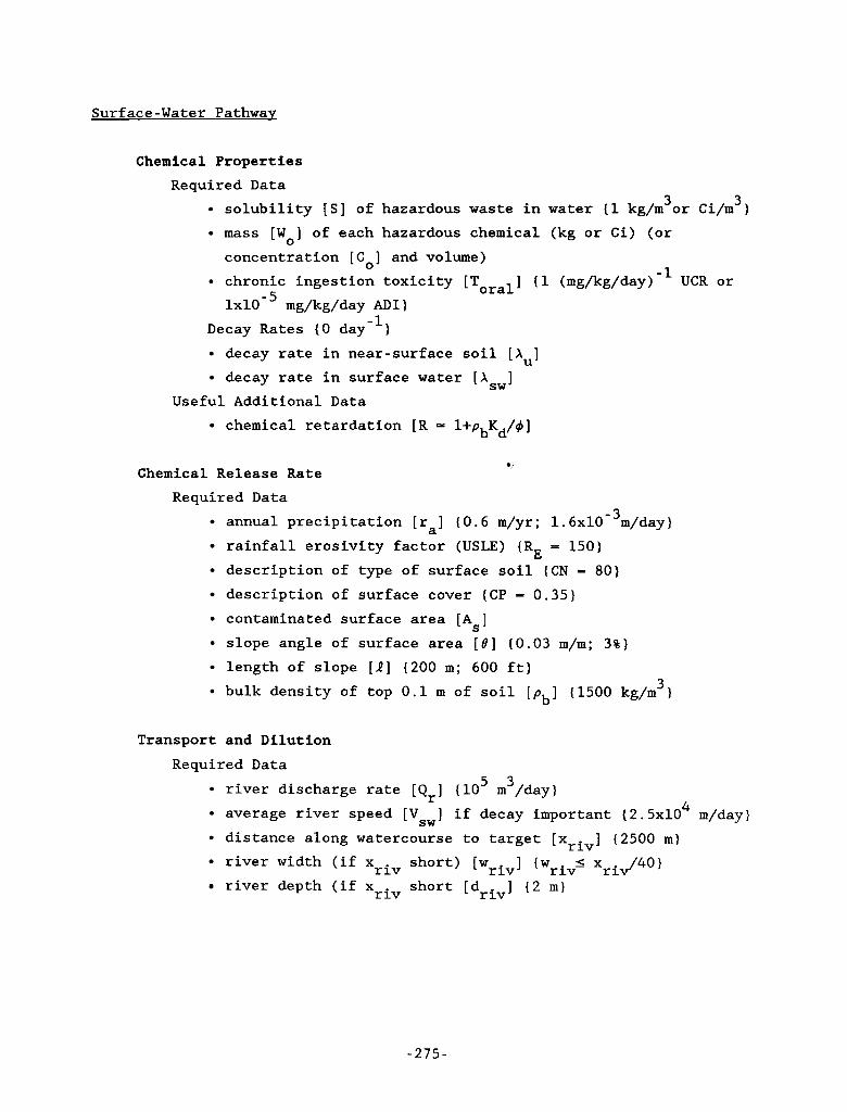
Surface-Water Pathway
Chemical Properties Required Data
3 3 solubility [SI of hazardous waste in water (1 kg/m or Ci/m 1 mass [W ] of each hazardous chemical (kg or Ci) (or
0 concentration [C ] and volume)
1 ~ 1 0 - ~ mg/kg/day AD1 I
0 chronic ingestion toxicity [T
Decay Rates ( 0 day-') decay rate in near-surface soil [ A ] decay rate in surface water [ A 3
] (1 (mg/kg/day)-' UCR or oral
U
sw Useful Additional Data
chemical retardation [R = l+pbKd/d]
Chemical Release Rate Required Data
3 annual precipitation [r,] (0.6 m/yr; 1.6~10- m/day) rainfall erosivity factor (USLE) (R = 150) description of type of surface soil (CN = 80) description of surface cover (CP - 0.35) contaminated surface area [A ]
slope angle of surface area [e] ( 0 . 0 3 m/m; 3 % )
length of slope [l] (200 m; 600 ft) bulk density of top 0.1 m of soil [pb] (1500 kg/m )
E
S
3
Transport and Dilution Required Data
5 3 river discharge rate [Q,] (10 m /day)
distance along watercourse to target [x ] (2500 m)
river width (if xriv short) [wriv] (writ xri ,,/40 I river depth (if xriv short [driv] (2 m)
average river speed [Vsw] if decay important (2.5~10 4 m/day)
r iv
-275-
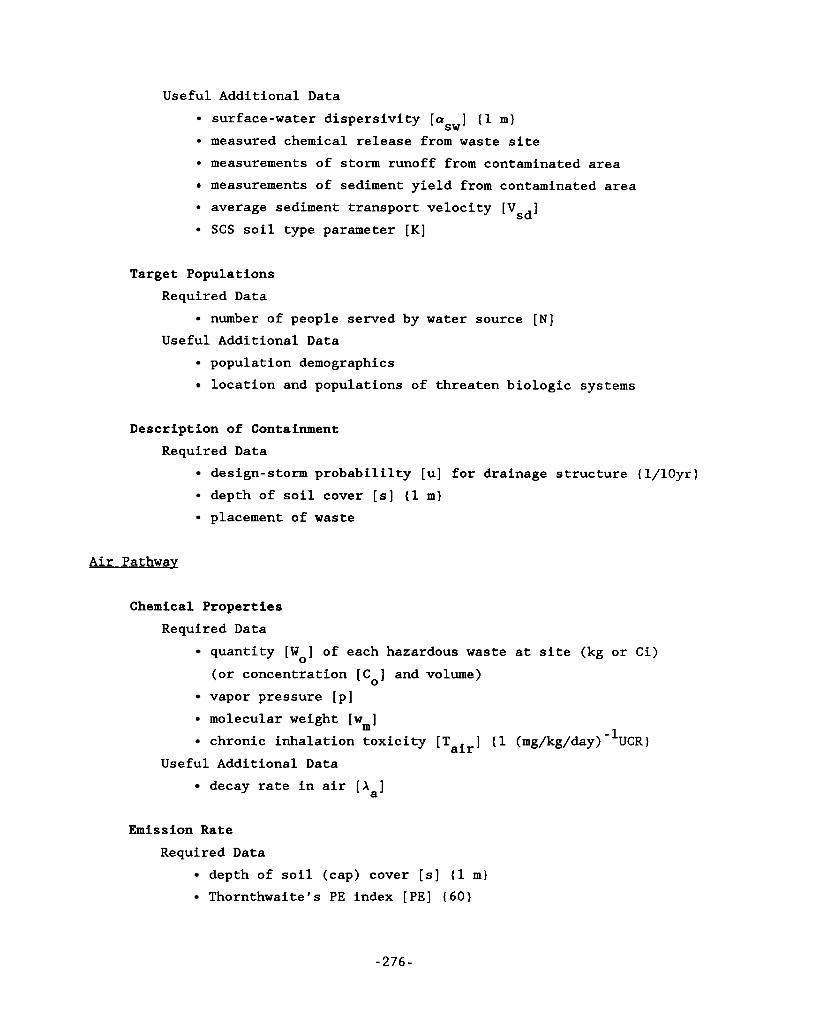
Useful Additional Data surface-water dispersivity [a ] (1 m) measured chemical release from waste site measurements of storm runoff from contaminated area measurements of sediment yield from contaminated area
average sediment transport velocity [V ] SCS soil type parameter [K]
sw
sd
Target Populations Required Data
number of people served by water source [N] Useful Additional Data
population demographics location and populations of threaten biologic systems
Description of Containment Required Data
design-storm probabililty [u] for drainage structure (l/lOyr) depth of soil cover [SI (1 m) placement of waste
Air Pathwav
Chemical Properties Required Data
quantity [Wo] of each hazardous waste at site (kg
vapor pressure [p] molecular weight [w ] chronic inhalation toxicity [Tair] (1 (mg/kg/day)
decay rate in air [Aa]
(or concentration [C ] and volume) 0
m
Useful Additional Data
or Ci)
'lUCR)
Emission Rate Required Data
depth of soil (cap) cover [SI (1 m) Thornthwaite's PE index [PE] (60)
-276-
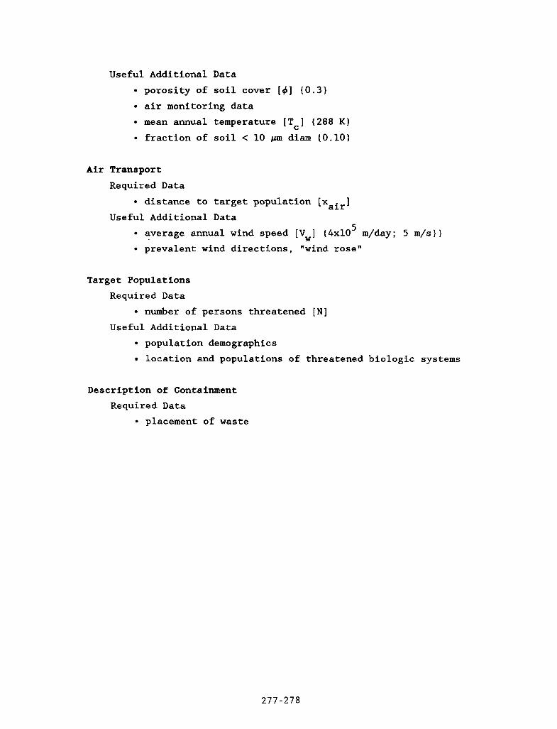
Useful Additional Data porosity of soil cover [ 4 ] (0.3) air monitoring data mean annual temperature [Tc] (288 K) fraction of soil < 10 put diam (0.10)
Air Transport Required Data
distance to target population [x ] air Useful Additional Data
5 average annual wind speed [V ] (4x10 m/day; 5 m/s)) W
prevalent wind directions, "wind rose"
Target Populations Required Data
number of persons threatened [N] Useful Additional Data
population demographics location and populations of threatened biologic systems
Description of Containment Required Data
placement of waste
c
- - -. ~ .- - . -- . . . ". . . . _. - . .
277-278
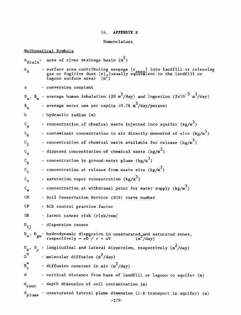
14. APPENDIX E
Nomenclature
Mathematical Symbols
*drain 2 - area of river drainage basin (m )
- surface area contributing seepage [r ] into landfill or releasing gas or fugitive dust [e] (usually eqE?%lent to the landfill or lagoon surface area) (m2>
* S
a - conversion constant 3 - 3 3 Ba, Bw - average human inhalation (20 m /day) and ingestion (2x10 m /day)
3 - average water use per capita (0.76 m /day/person) BU
b - hydraulic radius (m)
‘a 3 - concentration of chemical waste injected into aquifer (kg/m )
3 - contaminant concentration in air directly downwind of site (kg/m )
3 - concentration of chemical waste available for release (kg/m )
- disposed concentration of chemical waste (kg/m )
‘b
‘i
cO
C - concentration in ground-water plume (kg/m )
‘r
cV
cW
3
3 P
3 - concentration at release from waste site (kg/m )
- saturation vapor concentration (kg/m )
- concentration at withdrawal point for water supply (kg/m )
3
3
CN - Soil Conservation Service (SCS) curve number
CP - SCS control practice factor CR - latent cancer risk (risk/rem)
Dij
DU
- longitudinal and lateral dispersion, respectively (m 2 /day) Dx’ y
DC
d
dcont
dp lume
- dispersion tensor
- hydrodynamic dispsrsion in unsaturated and saturated zones, D gw respectively = VD / r + Crv (m2/day>
D 2 D* - molecular diffusion (m /day)
- diffusion constant in air (m /day)
- vertical distance from base of landfill or lagoon to aquifer (m)
- depth dimension of soil contamination (m) - unsaturated lateral plume dimension (1-D transport in aquifer) (m)
* 2
7 -279-

- mean river depth (m) dr iv DF , - ingestion and inhalation radionuclide human dose factors, D P 1 respectively (rem per pCi/day) air E - exposure; subscripts indicate whether from ground-water [gw],
surface-water [sw], or air [air] pathway (kg)
e - total emission rate into air pathway (kg/day) e e - emission rate of waste gas or fugitive dust into atmosphere (kg/day)
ETm
F - score of measured parameter (numerous subscripts)
v' w - monthly evapotranspiration
- factor evaluating soil cover for air pathway - subjective factor evaluating leachate collection practices
fcovr
fcllct f - engineered-barrier factor eng f fgen Put
frtrd
fsite
- factor increasing emission (if other gas present to sweep waste3 - subjective factor evaluating method of waste placement
- subjective factor for evaluating chemical retardation
- site reduction factor - subjective factor evaluating soil cover and hydraulic structures
s trct 2 g - acceleration of gravity (m/s )
- mass-loading adjustment for ground-water, surface-water, and air pathways ggw ' gsw
ga H - Henry's gas law constant
h - depth of soil susceptible to erosion
i
K - SCS soil erodibility factor
Kcovr
Kd K - hydraulic conductivity (Darcy flow) of aquifer (m /day)
3 - flow rate of leachate from site to aquifer (m /day) r
2 - hydraulic conductivity of cover over landfill (m /day) - partition or distribution coefficient (m /kg) 3
2 . gw
- vertical hydraulic conductivity of unsaturated zone between waste site and aquifer, Ku = Z.Li/(Z L./K.), where Ki is geologic stratum
i 1 1 hydraulic 2onductivity, f. is stratum thickness, and n is number of stratum (m /day)
KU
i
k - proportionality constant
-280-
A
k - volatilization mass transfer coefficient
- -
- container life before leaking (day)
- height of ith geologic stratum (m) LC
Li Q - length of slope (ft)
- length for thorough mixing in surface water (m) 'rn LS - length-slope factor in universal soil loss equation
M - total mass released from waste site (kg) M
Ma,Msw - average mass release rate from site (air and surface water) (g/day) m - aquifer thickness (m)
m - gram molecular weight
N - size of target (receptor) population
- average mass release rate from site per aquifer thickness (g/day/m) gw
W
n - number of atoms in 1 mg of isotope
n - Manning's coefficient (s/m V 3 ) m P - probability of scenario P - vapor pressure of volatile waste (atm) PE - Thornthwaite precipitation-effectiveness index
P(v*)
Qa
Qr -
Qw
- erosion potential, i.e., mass of erodible particles on surface 3 - additional clean water mixed with contaminated water (0 m /day)
- river discharge rate (m /day)
- withdrawal rate from aquifer (m /day)
- additional diluting surface runoff in intermittent stream (m /day)
3
3
3
q
QF - radiation quality factor
R - chemical retardation factor
- surface runoff discharge (m3/day)
- universal gas constant - SCS rainfall factor in universal soil loss equation
- human health risk, general ecological system risk, economic risk,
RC
RE
RS
A h
%,Re, respectively
-281-
r
r
r
r
r
S
a
m
net
perc
seep
s (Xi> A
s (R)
S
r iv S
T
TC
5/2 U
U
- average daily precipitation (m/day) - monthly precipitation (m/month)
- net precipitation runoff (m/day) - leachate release rate (m/day) - potential seepage into landfill or lagoon (m/day) - chemical solubility (kg/m )
- standard deviation of variable X
- standard deviation of risk prediction R
- depth of soil cover over the waste (m) - slope of surface water (m/m) - chronic toxicity of the chemical (either allowable dailylintake
- mean annual temperature (K) - average human life expectancy (2.56~10 day)
- half-life of hazardous material (day)
- probability that at least one storm event will exceed design storm frequency [u] over period t
3
i A
(ADI) (mg/kg/day) or unit cancer risk (UCR) (mg/kg/day)
4
R - design storm probability (reciprocal of design storm frequency)
V V - aquifer and percolation average interstitial water speed (m/day)
'sd
gw' u - river sediment speed (m/day) - surface water speed (m/day)
- mean annual wind speed (m/day) Vsw
VW * V - fastest mile of wind (m/s)
v* - river shear velocity (m/day)
- mass of hazardous waste deposited at site (kg) - mass of hazardous waste available for release (kg)
wO
'i W - body mass of average individual (70 kg)
"b W - unsaturated width of plume (1-dimensional transport in aquifer) (m)
W - river width (m)
- body mass of organ b (kg)
p lwne
r iv
- 2 8 2 -
A
- variable of R
- horizontal contaminant pathway distance from waste site to target population via ground-water, surface-water, and air pathway (m)
[R(Xi, ...,$ ) I 'i
gw 9 Xriv air
X X
i X
yS
'd
Y
Z
Z
a
r
6
e
rl
6
IC
x
5) 'dis
'covr
'r Y
< 'b U
r
4
i
- spatial coordinate - sediment yield from contaminated area (kg/m )
2
- contaminant yield after decay
- lateral distance (m) - activity of radionuclide per mg/kg body weight/day
- vertical distance (m)
- dispersivity (m) - constant for ground-water, surface-water, air pathways (gw, sw, and a subscripts)
- dilution of chemical waste along pathway
- effective absorbed energy [ e ] per disintegration of radionuclide in organ k, including a quality factor [QF] to convert rad to rem (MeV/dis rem/rad)
- hydraulic gradient - slope of surface contaminated with toxic waste (%)
- mass concentration [W./(pd A ) ] (kg/kg) 1 cont s
-1 - decay rate of material (numerous subscripts) (day )
- fraction of radionuclide absorbed in organ b
- runoff ratio, r netIra - portion of covered soil (varies from 0 for none to 1 for covered)
- fraction of annual precipitation percolating through waste dump
- constrictivity of porous media - energy absorbed per disintegration of radionuclide
- bulk density of soil
- atmospheric dispersion in x, y, or z direction (subscripts) (m /day)
- tortuosity in porous media
- porosity of material
- diffusion path distance (conceptual)
2
-283-
$ - consequence of a release scenario n - volume of waste (mixing cell volume) (m ) 3
- fractional contribution of organ b to the total risk under uniform whole-body irradiation "b
Acronyms and Initialisms
AD1 - Acceptable Daily Intake of noncarcinogens (RfD) (mg/kg/day) AEA - Atomic Energy Act of 1954 CAG - Carcinogen Assessment Group of EPA CERCLA - Comprehensive Environmental Response, Compensation, and Liability
Act (Superfund) of 1980; law applicable to abandoned waste sites
CPF - Carcinogenic Potency Factor; equivalent to UCR
CWA - Clean Water Act
DOE - U.S. Department of Energy EDE - Effective dose equivalent EPA - U.S. Environmental Protection Agency
FDA - Food and Drug Administration FS - Feasibility Study on Superfund sites
HARM - USAF Hazard Assessment Rating Methodology for hazardous waste sites
HAZWRAP- Hazardous Waste Remedial Action Program of DOE Defense Programs Undersecretary
HEA - EPA Health Effects Assessments documents HPI - Hazard Potential Index used in RAPS
HRS
mHRS - modified Hazard Ranking System; HRS modified by PNL to include
- Hazard Ranking System developed for EPA to rank sites for NPL
radionuclides
NOAEL - No Observed Adverse Effects Limit; used to establish AD1 NPL - National Priorities List; list of sites that may receive CERCLA
funding; established using HRS
NRC - U.S. Nuclear Regulatory Commission
ORNL - Oak Ridge National Laboratories, Oak Ridge, Tennessee
-284-
I..
PCBs
PNL
RAPS
RCRA
RfD
RI
SARA
scs SNLA
SRS
UCR
USAF
- Polychlorinated Biphenyl chemicals - Battelle Pacific Northwest Laboratories, Richland, Washington - Remedial Action Priority System under development by PNL
- Resource Conservation and Recovery Act of 1976; law applicable to current and future hazardous waste sites and handling practices
- EPA reference dose (ADI) (mg/kg/day) - Remedial investigation report of a waste site (EPA term) - Superfund Admendments and Reauthorization Act of 1986
- U.S. Soil Conservation Service - Sandia National Laboratories, Albuquerque, New Mexico - Site Ranking System developed by SNLA for ranking DOE hazardous waste sites
-1 - Unit Cancer Risk (mg or pCi/kg body weight/day) - U.S. Air Force
Definitions
Risk Assessment--Risk assessments estimate effects of substance or process on individuals or population
Risk Assessment policy--Risk assessment policy establishes philosophy used to select among analysis choices
Risk Management--Risk management is the process of evaluating and selecting alternative courses of action
285- 286
15. REFERENCES
A m , 1954. The Atomic Energy Act of 1954, Pub. L. No. 83-703, 68 Stat. 919.
Almanac, 1986. Information Please Almanac 1986, 40th Edition, (New York: A&W Publishers, Inc.).
Barfield, B. J., R. C. Warner, and C. T. Haan, 1981. Applied hydrology and sedimentology for disturbed areas, (Stillwater, OK: Oklahoma Technical Press), p. 311.
Barr, S . , and W. E. Clements, 1984. Diffusion modeling: Principles of application, in Atmospheric Science and Power Production, DOE/TIC-27601, D. Randerson, ed., Office of Scientific and Technical Information (OSTI), U.S. Dept. of Energy (DOE), pp. 589-94.
Bear, J., 1979. Hydraulics of Groundwater, (New York: McGraw-Hill).
BEIR, 1980. The effects on populations of exposure to low levels of ionizing radiation, Biological Effects of Ionizing Radiations (BE1R)--Advisory Committee, National Academy of Sciences, Washington, DC.
Boutwell, S . H., S . M. Brown, B. R. Roberts, and D. F. Atwood, 1985. Modeling remedial actions at uncontrolled hazardous waste sites, U.S. Environmental Protection Agency (EPA), prepared by Anderson-Nichols and Co., Palo Alto, CA.
Caldwell, S . , 1986. Staff member of U.S. Environmental Protection Agency (EPA), Office of Emergency and Remedial Response, quoted in Environment Reporter, Bureau of National Affairs (BNA), Washington, DC, September 12, 1986, p. 707.
CERCLA, 1980. Comprehensive Environmental Response, Compensation, and Liability Act of 1980, Pub. L. No. 96-510, 94 Stat. 2767.
Codell, R. B., K. T. Key, and G. Whelan, 1982. Collection of mathematical models for dispersion in surface water and groundwater, U.S. Nuclear Regulatory Commission (NRC), Washington, DC.
Cowherd, C., G. E. Muleski, P. J. Englehart, and D. A. Gillette, 1985. Rapid assessment of exposure to particulate emissions from surface contamination sites, EPA 600/8-85/002, Office of Health and Environmental Assessment, U.S. Environmental Protection Agency (EPA), prepared by Midwest Research Institute, Kansas City, MO.
Chow, V. T., 1959. Open-channel hydraulics, (New York: McGraw-Hill) pp. 115-23.
Chu, M.S.Y., J. V. Rodricks, C. St. Hilaire, and R. L. Bras, 1986. Risk assessment and ranking methodologies for hazardous chemical defense waste: A state-of-the-art review and evaluation, Task 1 Report, SAND86-0530, Sandia National Laboratories, Albuquerque, NM 87185.
Cranwell, R. M., J. E. Campbell, J. C. Helton, R. L. Iman, D. E. Longsine, N. R. Ortiz, G. E. Runkle, and M. J. Shortencarier, 1987. Risk methodology for geologic disposal of radioactive waste: Final report, NUREG/CR-2452, SAND81-2573, Sandia National Laboratories, Albuquerque, NM.
c -287-
CWA, 1977. Clean Water Act of 1977, Pub. L. No. 95-217, 91 Stat. 1566.
Delos, C. G., W. L. Richardson, J. V. Depinto, R. B. Ambrose, P. W. Rodgers, 1984. Technical guidance manual for performing waste load allocations, Book 2: Streams and rivers, Chapter 3: Toxic subtances, Office of Water Regulations and Standards, U.S. Environmental Protection Agency, Washington, DC.
Donigian, A. S . , T. Y. R. Lo, and E. W. Shanahan, 1983. Rapid assessment of potential ground-water contamination under emergency response conditions, U.S. Environmental Protection Agency (EPA), by Anderson-Nicholsflest, Palo Alto, CA.
EPA, 1986a. Superfund exposure assessment manual, DRAFT, OSWER Directive 9285.5-1, Office of Solid Waste and Emergency Response (OSWER), U.S. Environmental Protection Agency (EPA), prepared by Versar, Inc., Springfield, VA.
EPA, 1986b. Superfund public health evaluation manual, OSWER Directive 9285.4-1, Office of Solid Waste and Emergency Response, U.S. Environmental Protection Agency (EPA), prepared by ICF Incorporated, Washington, DC.
EPA, 1984a. Environmental progress and challenges: An EPA perspective, U.S. Environmental Protection Agency (EPA), Washington, DC.
EPA, 1984b. The RCRA risk-cost analysis model, Phase I11 report, DRAFT, Office of Solid Waste, U.S. Environmental Protection Agency (EPA), prepared by ICF Incorporated, Washington, DC.
EPA, 1983. Land disposal of hazardous waste, Proceedings of the Ninth Annual Research Symposium, EPA 600/9-83-018, U.S. Environmental Protection Agency (EPA), pp. 114-25.
EPA, 1982. Evaluation and selection of models for estimating air emissions from hazardous waste treatment, storage, and disposal facilities, Chapter 6, U.S. Environmental Protection Agency, prepared by GCA Corporation.
EPA, 1977. The report to Congress: Waste disposal practices and their effects on ground water, U.S. Environmental Protection Agency (EPA), Washington, DC., 531 pp.
Farmer, W. J., M. S. Yang, J. Letey, W. F. Spencer, and M. H. Roulier, 1978 Controlling vapor movement in Land disposal of hexachlorobenzene waste:
soils, Fourth Annual Symposium on Land Disposal, San Antonio, TX.
Fisher, H. B., 1967. The mechanics of dispersion in natural streams, J. Hydraul. Div., ASCE, V. 93, No. HY 6, pp. 187-216.
Freeze, R. A., and J. A. Cherry, 1979. Groundwater (Englewood Cliffs, NJ: Prentice-Hall, Inc.), p. 29.
FSC, 1980. Proposed system for food safety assessment, Final Report of the Scientific Committee of the Food Safety Council (FSC), Washington, DC.
Hawley, K. A., and B. A. Napier, 1985. A ranking system for sites with mixed radioactive and hazardous wastes, DRAFT, Pacific Northwest Laboratory, Richland, WA.
- 2 8 8 -
Helton, J. C., R. L. Iman, J. D. Johnson, and C. D. Leigh, 1986. Uncertainty and sensitivity analysis of a model for multicomponent aerosol dynamics, Nuclear Technology, V. 73, pp. 320-42.
HRS Workshop, 1982. Selection of hazardous waste sites for superfund funding, Workshop transcripts, sponsored by Subcommittee on Department of Housing and Urban Development-Independent Agencies of the Committee on Appropriations, U.S. Senate, U.S. Printing Office, Washington, DC, March 19-20, 1982.
Hoffman, F. O., and R. H. Gardner, 1983. Evaluation of uncertainties in radiological assessment models, in Radiological Assessment, a Textbook on Environmental Dose Analysis, J. E. Till and H. R. Meyer, eds., U.S. Nuclear Regulatory Commission (NRC), Washington, DC 20555
Hubbard, E. F., F. A. Kilpatrick, L. A. Martens, and J. F. Wilson, 1982. Measurement of time of travel and dispersion in streams by dye tracing, Chapter A9, in Techniques of Water-Resources Investigations of the United States Geological Survey, Book 3, Applications of Hydraulics, U.S. Geological Survey, Washington, DC.
ICRP, 1979. Limits for intake of radionuclides by workers, ICRP Publication 30, Part 1, Annals of ICRP 2 No. 3/4, Supplement to Part 1, Annals of the ICRP 3, No. 1-4 (New York: Pergamon Press)
Iman, R. L., J. C. Helton, 1985. A comparison of uncertainty and sensitivity analysis techniques for computer models, SAND84-1461, Sandia National Laboratories, Albuquerque, NM.
Iman, R. L., J. C. Helton, and J. E. Campbell, 1981a. An approach to sensitivity analysis of computer models, part 1: Introduction, input variable selection and preliminary variable assessment, J. of Quality Technology, V. 13, No. 3, pp. 174-83.
Iman, R. L., J. C. Helton, and J. E. Campbell, 1981b. An approach to sensitivity analysis of computer models, part 2 : Ranking of input variables, response surface validation, distribution effect and technique synopsis, J. Quality Technology, V. 13, No. 4, pp. 232-40.
Javandel, I., C. Daughty, and C. F. Tsang, 1984. Groundwater Transport: Handbook of Mathematical Models, Water Resources Monograph No. 10, (Washington, DC: Amer. Geophysical Union), p. 9.
Kufs, C., D. Twedell, S. Paige, R. Wetzel, P. Spooner, R. Colonna, and M. Kilpatrick, 1980. Rating the hazard potential of waste disposal facilities, In Proceedings on the Management of Uncontrolled Hazardous Wastes Sites, U.S. Environmental Protection Agency National Conference. Hazardous Materials Control Research Institute, Washington, DC, pp. 30-41.
Lacey, G., 1930. Stable channels in alluvium, Proc. Inst. Civil Eng., V. 229, pp. 259-92.
Lazar, E. C., R. Testani, and A. B. Giles, 1976. The potential for national health and environmental damages from industrial residue disposal, presented at National Conference on Disposal of Residues on Land, St. Louis, MO, September 15, 1976, 21 pp.
LeGrand, H. E., 1964. System for evaluation of contamination potential of some waste disposal sites, J. Am. Water Works, V. 56, pp. 959-74.
LEAF v. Hodell, 1984. Legal Environmental Assistance Foundation v. Hodell, 586 F. Supp. 1163 (1984).
Leopold, L. B., and J. P. Miller, 1956. Ephemeral streams--hydraulic factors and their relation to the drainage net, U.S. Geol. Survey Prof. Paper 282-A.
Lindley, E. S., 1919. Regime channels, Proc. Punjab Engineering Congress, V 7, pp. 63-74.
Lyon, T. L., H. 0. Buckman, and N. C. Brady, 1957. The Nature and Properties of Soils, (New York: Macmillan, Inc.).
Mackay, D., 1980. Solubility, partition coefficients, volatility, and evaporation rates, in The Handbook of Environmental Chemistry, V. 2, 0 . Hutzinger, ed. (New York: Springer-Verlag), pp. 31-45.
McKay, M. D., W. J. Conover, and R. J. Beckman, 1979. A comparison of three methods for selecting values of input variables in the analysis of output from a computer code, Technometrics, V. 21, No. 2.
Perry, R., and C. Chilton, 1973. Chemical Engineers Handbook, 5th ed. (New York: McGraw-Hill).
Pettyjohn, W. A., D. C. Kent, T. A. Prickett, H. E. Legrand, and F. E. Wite, Methods for the prediction of leachate plume migration and mixing, 1982.
U.S. Environmental Protection Agency (EPA), Municipal Environmental Research Laboratory, Cincinnati, OH.
Pickens, J. F. and G. E. Grisak, 1981. Modeling of scale-dependent dispersion in hydrogeologic systems, Water Resources Research, V. 17, NO. 6, pp. 1701-11.
Piver, W. T., and F. T. Lindstrom, 1984. Simplified estimation technique for organic contaminant transport in groundwater, J. Hazardous Materials, V. 8, pp. 331-9.
NCC, 1979. Climatic Atlas of the United States, National Climatic Center (NCC), U.S. Department of Commerce, Ashville, NC.
NRC, 1981. Draft environmental impact statement on 10 CFR Part 61 "Licensing requirements for land disposal of radioactive waste," U.S. Nuclear Regulatory Commission (NRC), Washington, DC, September 1981.
RCRA, 1976. Resource Conservation and Recovery Act of 1976 (RCRA), Pub. L. No. 94-580, 90 Stat. 2795.
Rechard, R. P., and V. R. Hasfurther, 1980. The use of meander parameters in the restoration of mined stream beds in the Eastern Powder River Basin, Water Resources Research Institute, University of Wyoming, Laramie, WY.
Richards, K. S . , 1982. Rivers Form and Process in Alluvial Channels (New York: Methuen, Inc.) pp. 276-301.
Risk Assessment in the Federal Government, 1983. National Research Council, (Washington, DC: National Academy Press), 191 p.
-290-
Rodricks, J. V., 1984. Risk assessment at hazardous waste disposal sites, J. Hazardous Waste, V. 1, pp. 333-62.
Rodricks, J. V., J. M. Brett, and G. C. Wrenn, 1987. Significant risk decisions in federal regulatory agencies, submitted to J. Regulatory Toxicology and Pharmacology.
Runkle, G. E., R. M. Cranwell, and J. D. Johnson, 1981. Risk methodology for geologic disposal of radioactive waste: NUREG/CR-2166, SAND80-1372, Sandia National Laboratories, Albuquerque, NM.
Dosimetry and health effects,
Sax, N. I., 1975. Dangerous Properties of Industrial Materials, 5th ed., (New York: Van Nostrand/Rheinhold Co.).
SARA, 1986. Superfund Amendments and Reauthorization Act (SARA) of 1986, Pub. L. No. 99-499, October 17, 1986.
Shen, T. T., 1981. Estimating hazardous air emissions from disposal sites, Pollution Engineering, V. 13, No. 7, pp. 31-34.
Skidmore, E. L., N. P. Woodruff, 1968. Wind erosion forces in the United States and their use in predicting soil loss. Agriculture Handbook No. 346, Agricultural Research Service, U.S. Dept. of Agriculture (USDA), Washington, DC.
Strahler, A. N., 1964. Geology Part 11. Quantitative Geomorphology of Drainage Basins and Channel Networks, in Handbook of Applied Hydrology, Ven Te Chow, ed., (New York: McGraw-Hill), p. 4-54.
Thibodeaux, L. J., 1981. Estimating the air emissions of chemicals from hazardous waste landfills, J. Hazardous Materials, V. 4, pp. 235-44.
Thibodeaux, L. J., C. Springer, and L. M. Riley, 1982. Models of mechanisms for the vapor phase emission of hazardous chemicals from landfills, J. Hazardous Materials, V. 7, pp. 63-74.
Todd, D. K., 1970. The water encyclopedia, Water Information Center, Port Washington, NY.
Tomovic, R., 1963. Sensitivity Analysis of Dynamic Systems, (New York: McGraw-Hill)
USAF, 1983. Installation restoration program, Phase I--Records search, Lowry AFB, Colorado, AFESC/DEV, United States Air Force, Tyndall AFB, FL.
USBR, 1977. Design of small dams, U.S. Dept. of Interior, Bureau of Reclamation, Washington, DC, p. 527.
c
van Genuchten, M. T., and W. J. Alves, 1982. Analytical solutions of the one-dimensional convective-dispersive solute transport equation, Technical Bulletin No. 1661, U.S. Dept. of Agriculture, p. 56.
Verschueren, K., 1984. Handbook of Environmental Data on Organic Chemicals, (New York: Van Nostrand/Reinhold Press).
-291-
Walton, W. C., 1984. Handbook of analytical ground water models, International Ground Water Modeling Center, Butler University, Indianapolis, Indiana, p. 11.5.
Weber, W. J., 1972. Physiochemical Processes for Water Quality Control, (New York: Wiley Interscience), p. 42.
Whelan, G., B. L. Steelman, D. L. Strenge, and J. G. Droppo, 1986. Overview of the remedial action priority system (RAPS), in Pollutants in a Multimedia Environment, Y. Cohen, ed., (New York: Plenum Publishing Corporation), pp. 191-227
Whelan, G., D. L. Strenge, B. L. Steelman, K. A. Hawley, 1985. Development of the remedial action priority system: An improved risk assessment tool for prioritizing hazardous and radioactive-mixed waste disposal sites, in Proceedings of Management of Uncontrolled Hazardous Waste Sites, Hazardous Materials Control Research Institute, Silver Spring, MD, November 4-6, 1985, pp. 432-7.
Wiest, J. D., and F. K. Levy, 1977. A management guide to PERT/CPM, 2nd ed., (Englewood Cliffs, NJ: Prentice-Hall).
Wilson, J. L . , and P. J. Miller, 1978. Two-dimensional plume in uniform ground-water flow, J. Hydraul. Div., ASCE, V. 104, No. 4, pp. 503-514.
10CFR20. Standards for protection against radiation, U.S. Nuclear Regulatory Commission (NRC), Title 10 Code of Federal Regulations Part 20 (10CFR20).
10CFR60. Disposal of high-level radioactive wastes in geologic repositories, technical criteria, U.S. Nuclear Regulatory Commission (NRC), Title 10 Code of Federal Regulations Part 60 (10CFR60).
10CFR61. Licensing requirements for land disposal of radioactive waste, U.S. Nuclear Regulatory Commission (NRC), Title 10 Code of Federal Regulations Part 61 (10CFR61).
40CFR190. Environmental radiation protection standards for nuclear power operations, U.S. Environmental Protection Agency (EPA), Title 40 Code of Federal Regulations Part 190 (40CFR190).
40CFR191. Environmental radiation protection standards for management and disposal of spent nuclear fuel, high-level and transuranic radioactive wastes, U.S. Environmental Protection Agency (EPA), Title 40 Code of Federal Regulations Part 191 (40CFR191).
40CFR264. Standards for owners and operators of hazardous waste treatment, storage, and disposal facilities, U.S. Environmental Protection Agency (EPA), Title 40 Code of Federal Regulations Part 264 (40CFR264).
40CFR267. Interim standards for owners and operators of new hazardous waste land disposal facilities, U.S. Environmental Protection Agency (EPA), Title 40 Code of Federal Regulations Part 267 (40CFR267).
40CFR300. Uncontrolled hazardous waste site ranking system; a user's manual, U.S. Environmental Protection Agency (EPA), Title 40 Code of Federal Regulations Part 300 (40CRF300), Appendix A.
-292-
DISTRIBUTION
XI.
I-
-
c
U.S. Department of Energy (3) Washington, DC 20545 Attn: C. H. George, DP-124
T. Longo, DP-124 G. H. Daly, DP-123
U.S. Department of Energy ( 4 ) Washington, DC 20585 Attn: J. C. Tseng, EH-23
U.S. Department of Energy (3) Albuquerque Operations P.O. Box 5400 Albuquerque, NM 87185 Attn: G. Runkle
C. Soden R. M. Ostmeyer
U.S. Department of Energy Oak Ridge Operations P.O. Box E Oak Ridge, TN 37831 Attn: R. C. Sleeman
Martin Marietta Energy Systems, Inc. (19) P.O. Box Y Bldg 9108, M/S 2 Oak Ridge, TN 37831 Attn: R. E. Adams
J. L. Epler (3) L. D. Eyman C. S. Fore J. F. McBrayer J. C. Parker N. E. Rothermich HAZWRAP Library (10)
Martin Marietta Energy Systems, Inc. (5) P.O. Box Y Oak Ridge, TN 37831 Attn: Central Research Library
Document Reference Section Laboratory Records Patent Office
-293-
Sandia National Laboratories
3314 G . J. Smith 3314 S. A. Felicetti 3314 G. E. Millard 3314 J . M. Phelan 6 3 1 2 R. W. Prindle 6 3 3 0 W. D. Weart- 6 3 3 1 R. L. Beauheim 6 3 3 1 M. D. Siege1 6 3 3 4 D. R. Anderson 6 3 3 4 M. S . Y. Chu ( 2 0 ) 6 3 3 4 R. L. Hunter 6 3 3 4 R. P. Rechard ( 2 0 ) 6 4 0 0 D. J. McCloskey 6 4 1 0 N. R. Ortiz ( 2 ) 6415 R. M. Cranwell ( 5 ) 6415 G. F. Wilkinson 6416 E. J. Bonano 6416 P. A . Davis 6416 C. D. Leigh 6416 L. R. Shipers 8 0 2 4 P. W. Dean 8 2 6 3 K. A. Siegfriedt 3 1 4 1 S . A. Landenberger ( 5 ) 3 1 5 1 W. L. Garner ( 3 ) 3 1 5 4 - 3 C . Dalin ( 5 7 )
for DOE/OSTI (Unlimited Release; UC
- 2 9 4 -


![SRS-01 SRS-02 Encoder 4MPX-ASI Decoder ASI-4MPXUserManuals~SRS_[EN].pdf · SRS-02 Encoder 4MPX-ASI Decoder ASI-4MPX ... The package should contain: a. SRS-01. b. ... The SRS-02, as](https://img.pdfslide.net/doc/110x75/5abb735f7f8b9a441d8cd573/srs-01-srs-02-encoder-4mpx-asi-decoder-asi-usermanualssrsenpdfsrs-02-encoder.jpg)