Embed Size (px)
DESCRIPTION
Â
Citation preview
Virtual University of PakistanLecture No. 34 of the course on
Statistics and Probability
by
Miss Saleha Naghmi Habibullah
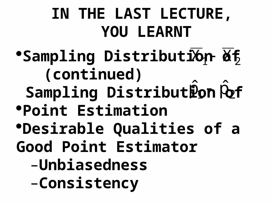
IN THE LAST LECTURE, YOU LEARNT
Sampling Distribution of (continued) Sampling Distribution of Point EstimationDesirable Qualities of a Good Point Estimator
–Unbiasedness–Consistency
21 p̂p̂
21 XX
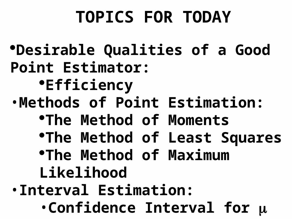
TOPICS FOR TODAY
Desirable Qualities of a Good Point Estimator:
Efficiency•Methods of Point Estimation:
The Method of MomentsThe Method of Least SquaresThe Method of Maximum Likelihood
•Interval Estimation:•Confidence Interval for
The students will recall that, in the last lecture, we presented the basic definition of a point estimator, and considered some desirable qualities of a good point estimator.
Three main qualities of a good point estimator are:
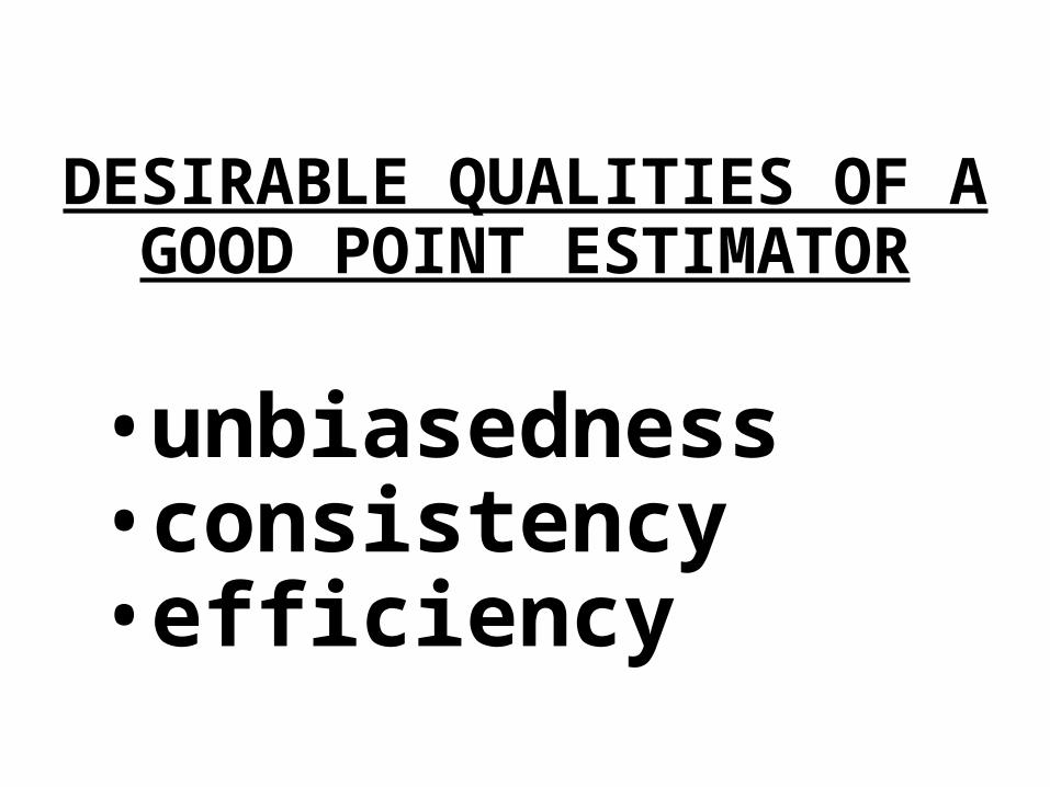
DESIRABLE QUALITIES OF A GOOD POINT ESTIMATOR
•unbiasedness•consistency•efficiency

In the last lecture, we discussed in some detail the concepts of unbiasedness and consistency.
Why is consistency considered a desirable quality?
In order to obtain an idea regarding the answer to this question, consider the following:
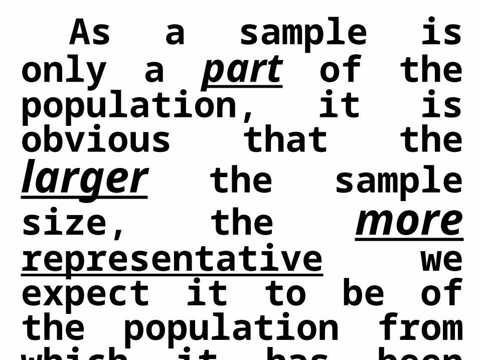
As a sample is only a part of the population, it is obvious that the larger the sample size, the more representative we expect it to be of the population from which it has been drawn.
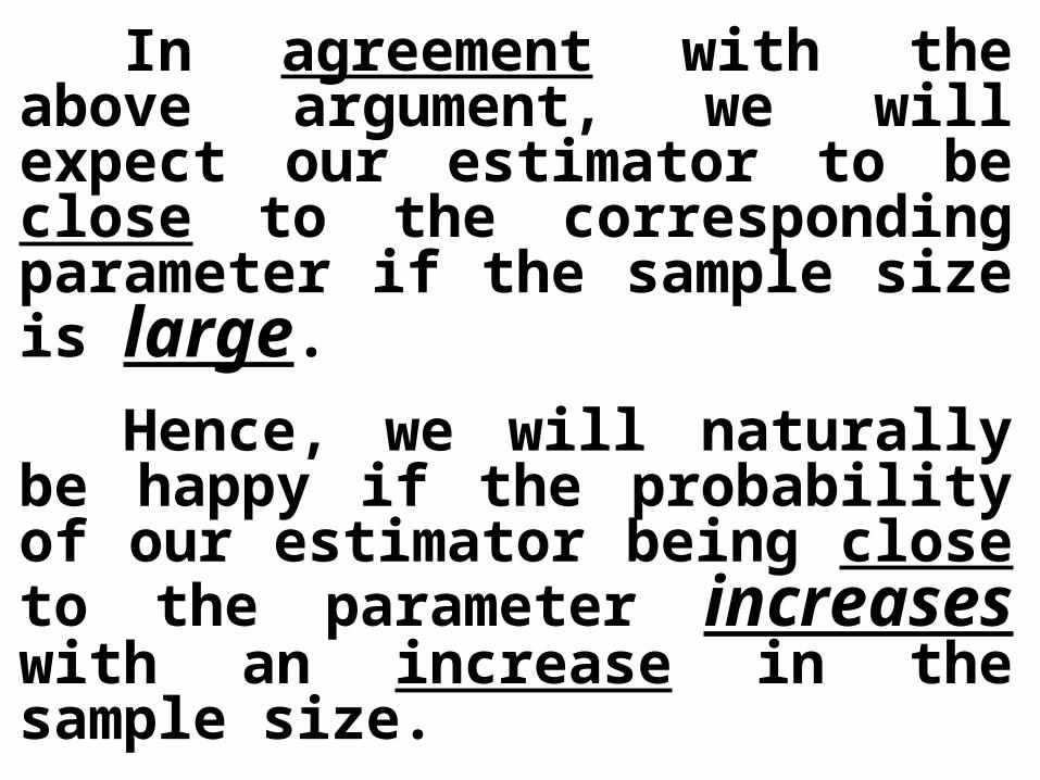
In agreement with the above argument, we will expect our estimator to be close to the corresponding parameter if the sample size is large.
Hence, we will naturally be happy if the probability of our estimator being close to the parameter increases with an increase in the sample size.
As such, consistency is a desirable property.

Another important desirable quality of a good point estimator is EFFICIENCY:
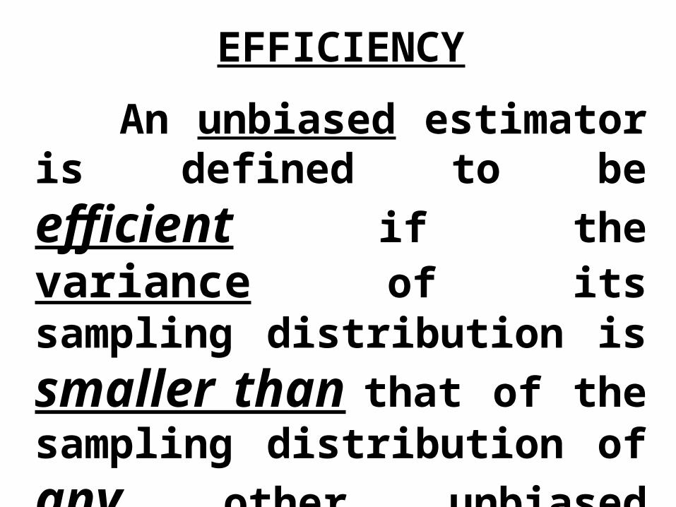
EFFICIENCY
An unbiased estimator is defined to be efficient if the variance of its sampling distribution is smaller than that of the sampling distribution of any other unbiased estimator of the same parameter.
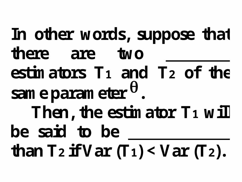
In other words, suppose thatthere are two unbiased estimators T1 and T2 of thesame parameter . Then, the estimator T1 willbe said to be more efficient than T2 if Var (T1) < Var (T2).
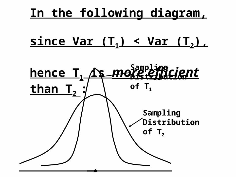
Sampling Distribution of T1
Sampling Distribution of T2
In the following diagram, since Var (T1) < Var (T2), hence T1 is more efficient than T2 :
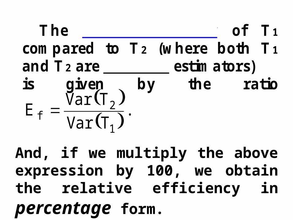
T h e rela tive efficien cy o f T 1 com p ared to T 2 (w h ere b oth T 1an d T 2 are u n b iased estim ators) is g iven b y th e ratio
.TVarTVarE
1
2f
And, if we multiply the above expression by 100, we obtain the relative efficiency in percentage form.
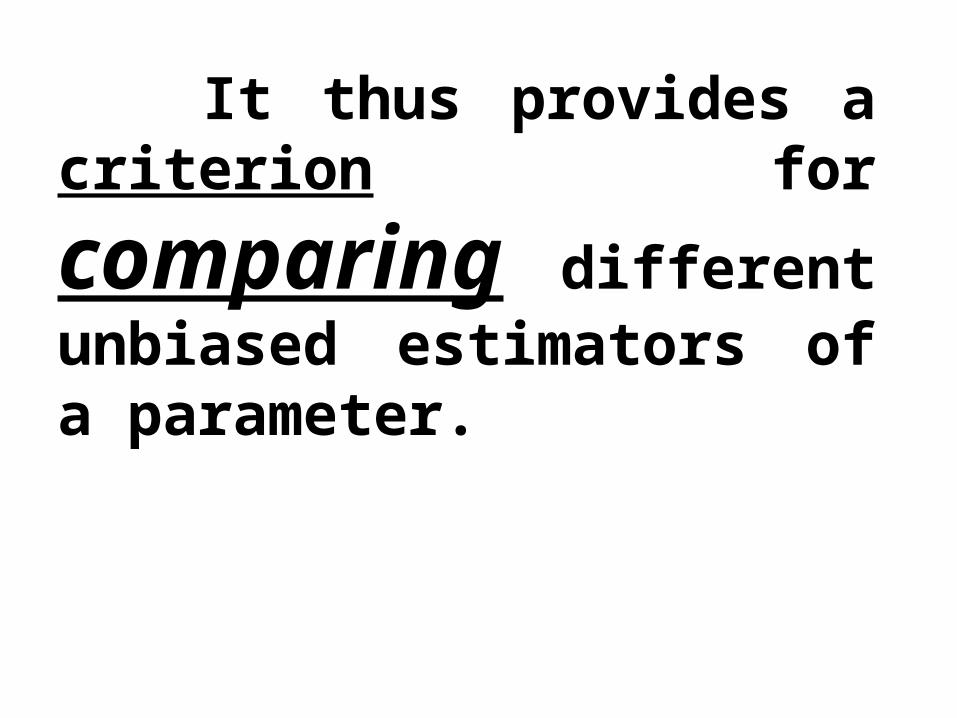
It thus provides a criterion
for comparing different unbiased estimators of a parameter.
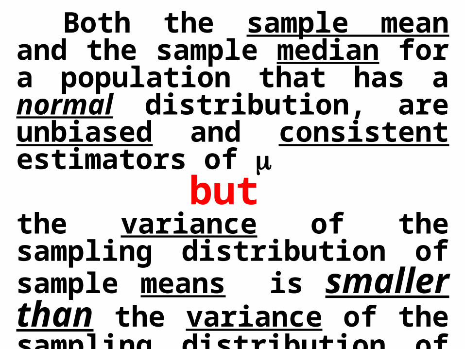
Both the sample mean and the sample median for a population that has a normal distribution, are unbiased and consistent estimators of
but the variance of the sampling distribution of sample means is smaller than the variance of the sampling distribution of sample medians.
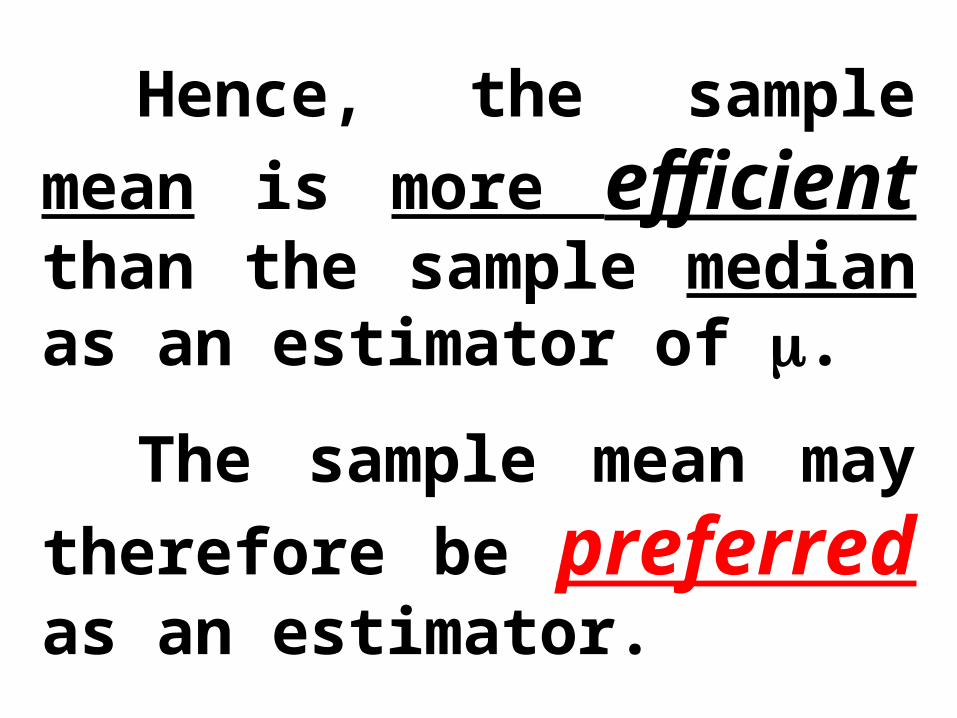
Hence, the sample mean is more efficient than the sample median as an estimator of .
The sample mean may therefore be preferred as an estimator.
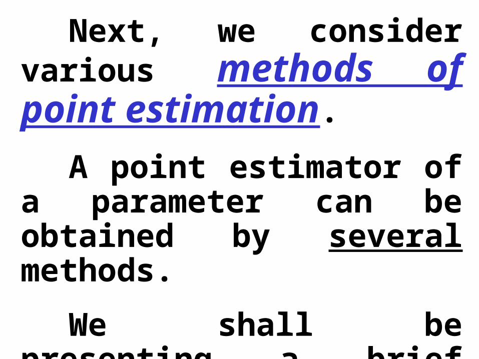
Next, we consider various methods of point estimation.
A point estimator of a parameter can be obtained by several methods.
We shall be presenting a brief account of the following three methods:
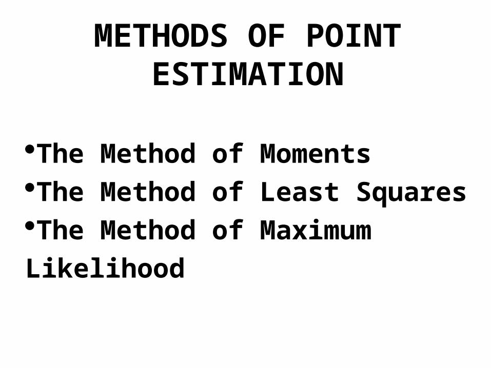
METHODS OF POINTESTIMATION
The Method of MomentsThe Method of Least SquaresThe Method of Maximum Likelihood
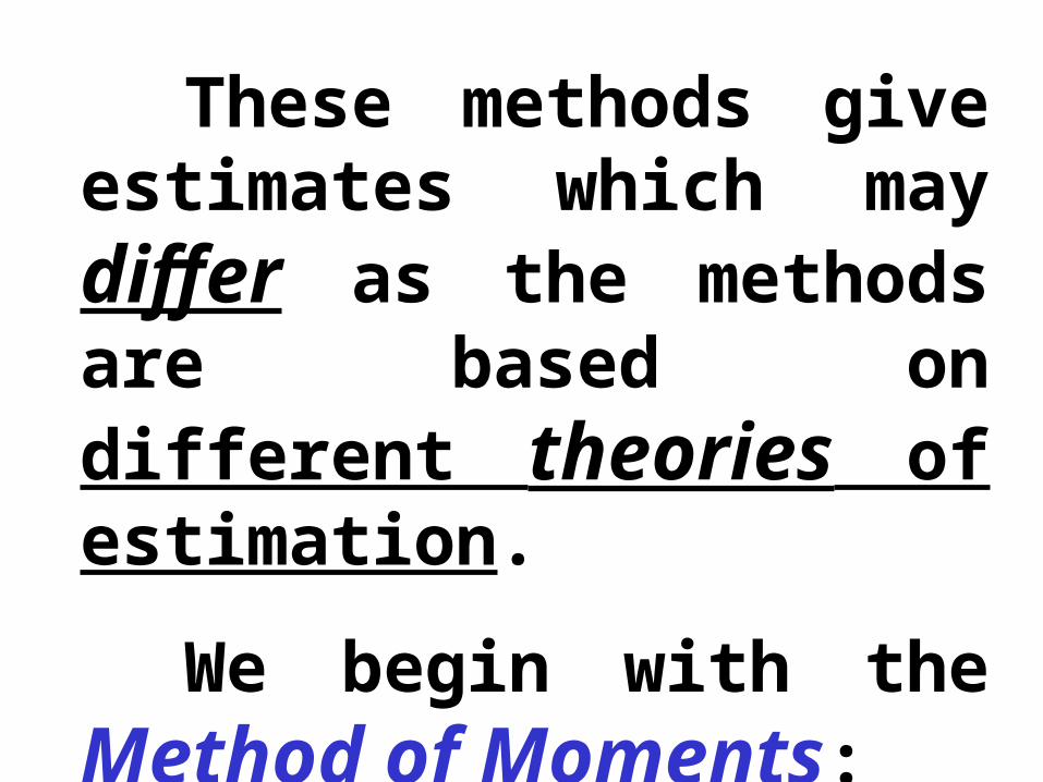
These methods give estimates which may differ as the methods are based on different theories of estimation.
We begin with the Method of Moments:
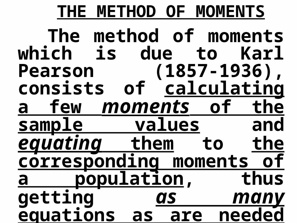
THE METHOD OF MOMENTSThe method of moments
which is due to Karl Pearson (1857-1936), consists of calculating a few moments of the sample values and equating them to the corresponding moments of a population, thus getting as many equations as are needed to solve for the unknown parameters.
The procedure is described below:
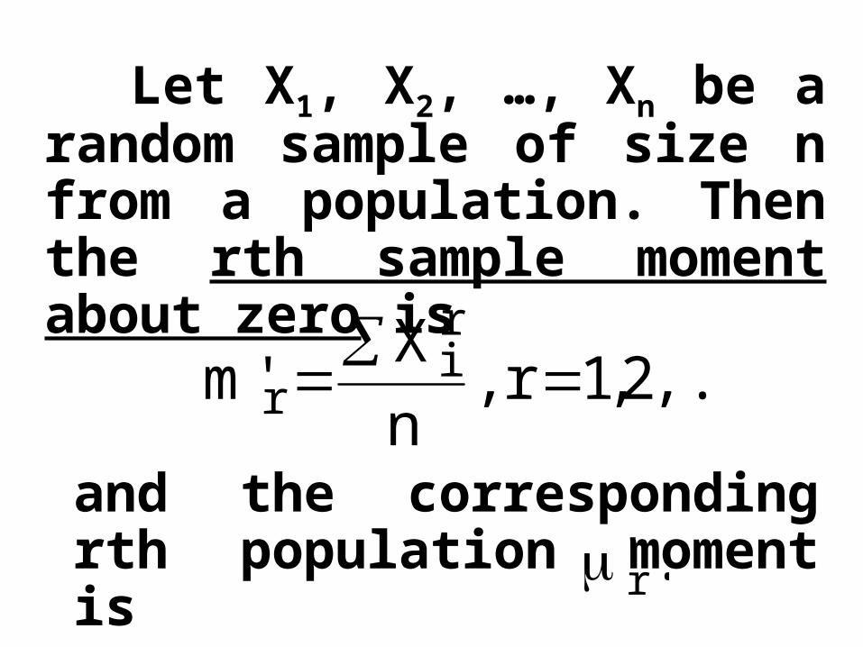
Let X1, X2, …, Xn be a random sample of size n from a population. Then the rth sample moment about zero is
,...2,1r,nX'm
ri
r
and the corresponding rth population moment is .'r
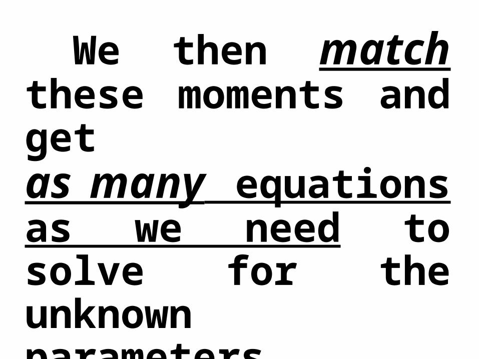
We then match these moments and get as many equations as we need to solve for the unknown parameters.
The following examples illustrate the method:
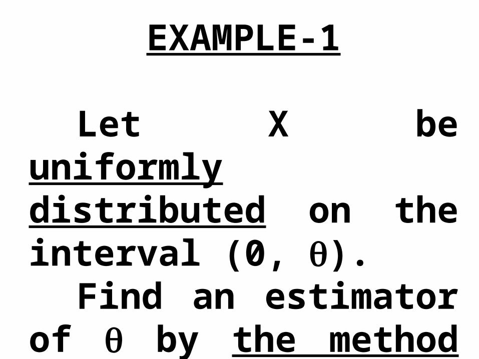
EXAMPLE-1
Let X be uniformly distributed on the interval (0, ).
Find an estimator of by the method of moments.
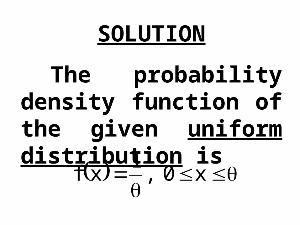
SOLUTION
The probability density function of the given uniform distribution is
x0,1xf
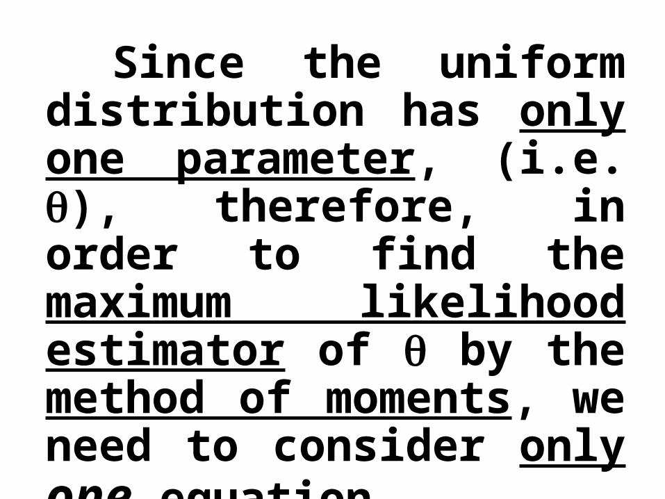
Since the uniform distribution has only one parameter, (i.e. ), therefore, in order to find the maximum likelihood estimator of by the method of moments, we need to consider only one equation.
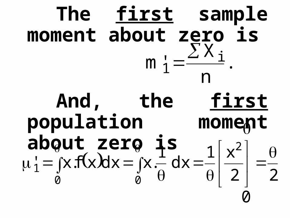
The first sample moment about zero is
And, the first population moment about zero is
.nX'm i
1
2
02
x1dx1.xdxxf.x'2
001
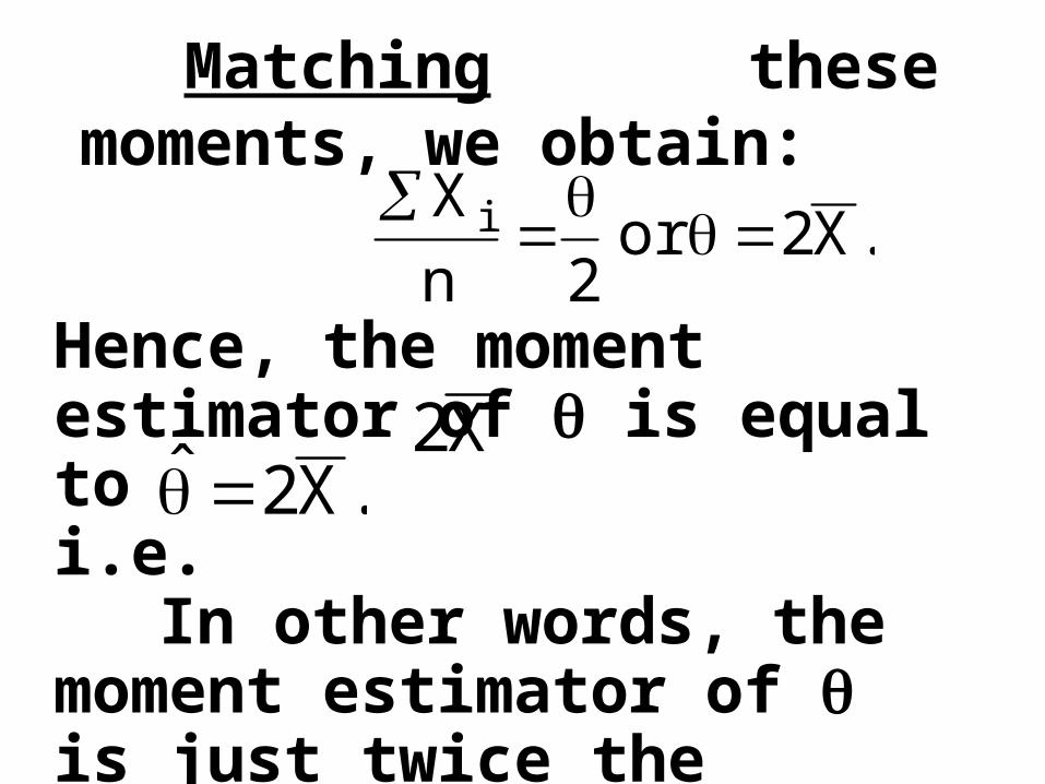
Hence, the moment estimator of is equal to i.e.
In other words, the moment estimator of is just twice the sample mean.
.X2or2n
Xi
Matching these moments, we obtain:
.X2ˆ X2
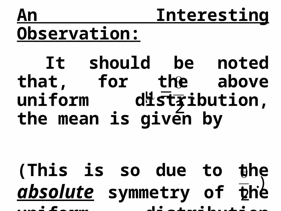
An Interesting Observation:
It should be noted that, for the above uniform distribution, the mean is given by
(This is so due to the absolute symmetry of the uniform distribution around the value
.2
).2
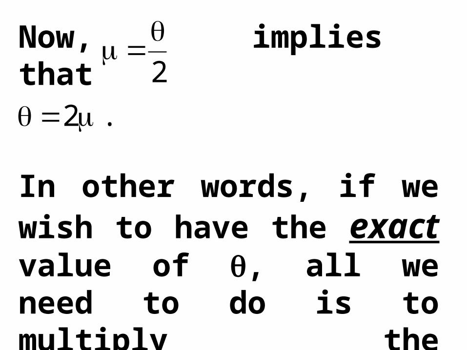
Now, implies that
In other words, if we wish to have the exact value of , all we need to do is to multiply the population mean by 2.
2
.2
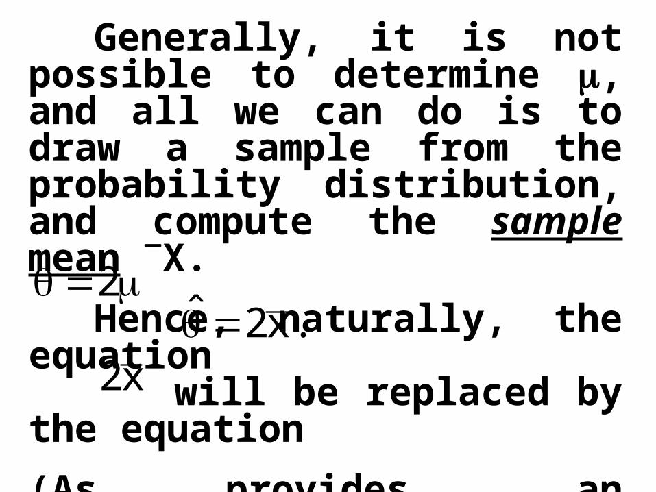
Generally, it is not possible to determine , and all we can do is to draw a sample from the probability distribution, and compute the sample mean X.
Hence, naturally, the equation will be replaced by the
equation(As provides an estimate of , hence a ‘hat’ is placed on top of .)
2.x2ˆ
x2
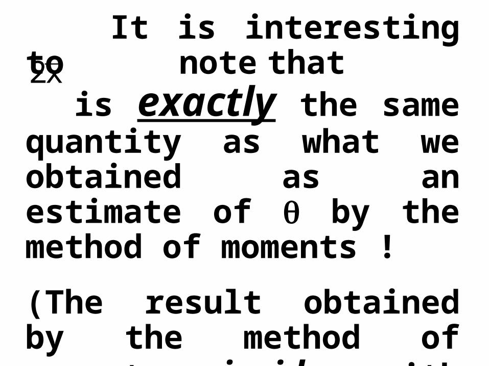
It is interesting to note that is exactly the same
quantity as what we obtained as an estimate of by the method of moments !
(The result obtained by the method of moments coincides with what we obtain through simple logic.)
x2
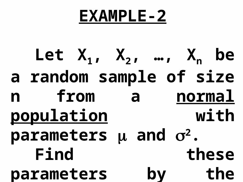
EXAMPLE-2
Let X1, X2, …, Xn be a random sample of size n from a normal population with parameters and 2.
Find these parameters by the method of moments.
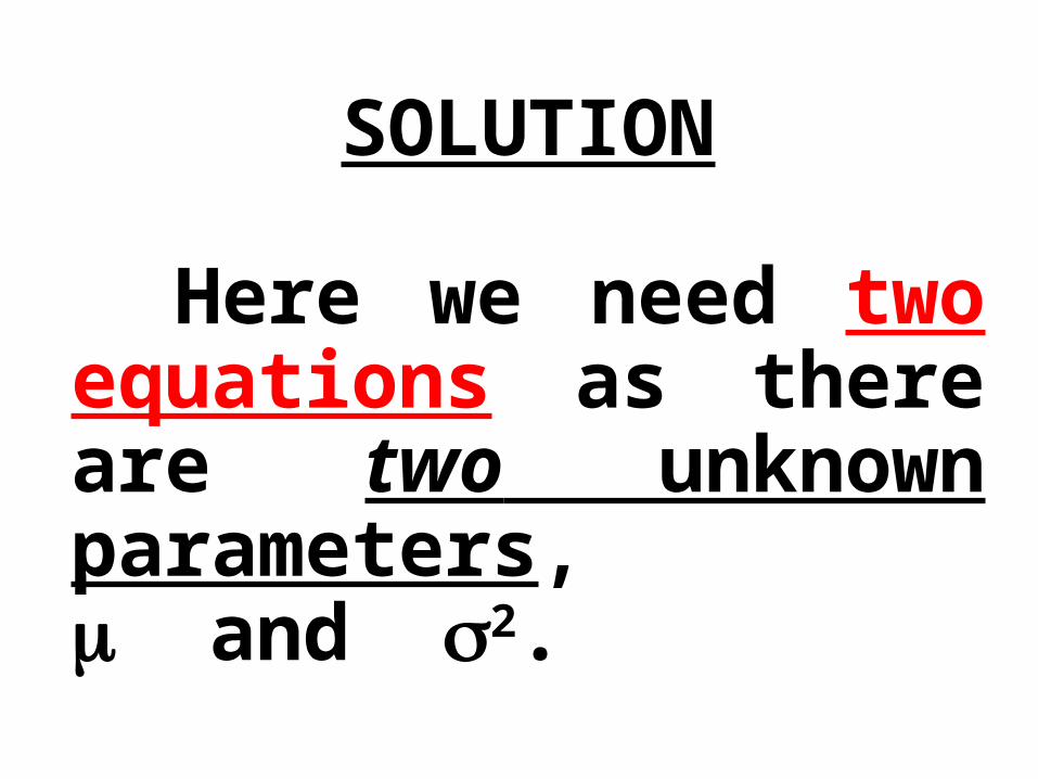
SOLUTION
Here we need two equations as there are two unknown parameters, and 2.
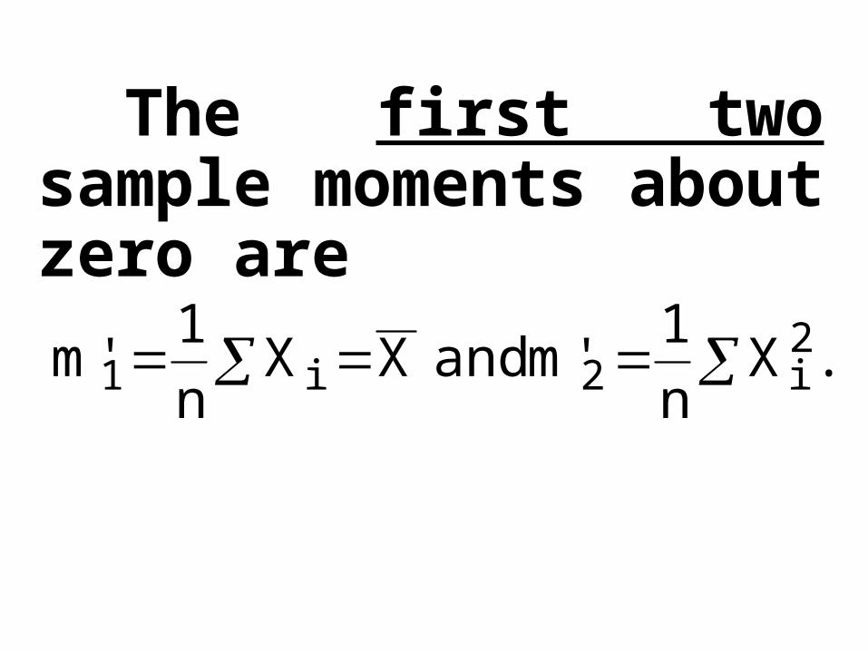
The first two sample moments about zero are
.Xn1'mandXX
n1'm 2
i2i1
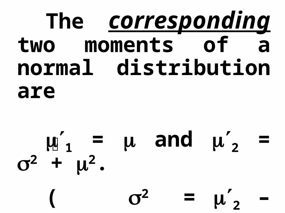
The corresponding two moments of a normal distribution are
1 = and 2 = 2 + 2.( 2 = 2 – 1
2
= 2 – 2 )
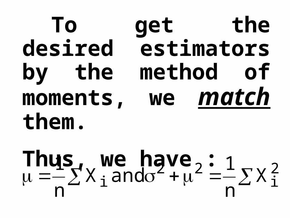
To get the desired estimators by the method of moments, we match them.
Thus, we have :
2i
22i X
n1andX
n1
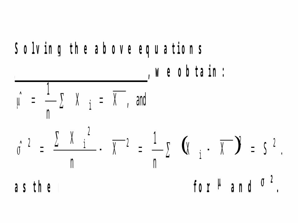
S o l v i n g t h e a b o v e e q u a t i o n ss i m u l t a n e o u s l y , w e o b t a i n :
and,XXn1ˆ i
.SXXn1X
nXˆ 22
i2
2i2
a s t h e m o m e n t e s t i m a t o r s f o r a n d 2 .
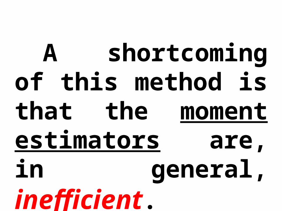
A shortcoming of this method is that the moment estimators are, in general, inefficient.
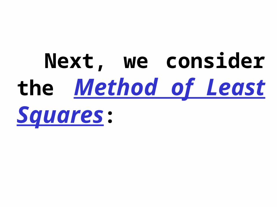
Next, we consider the Method of Least Squares:
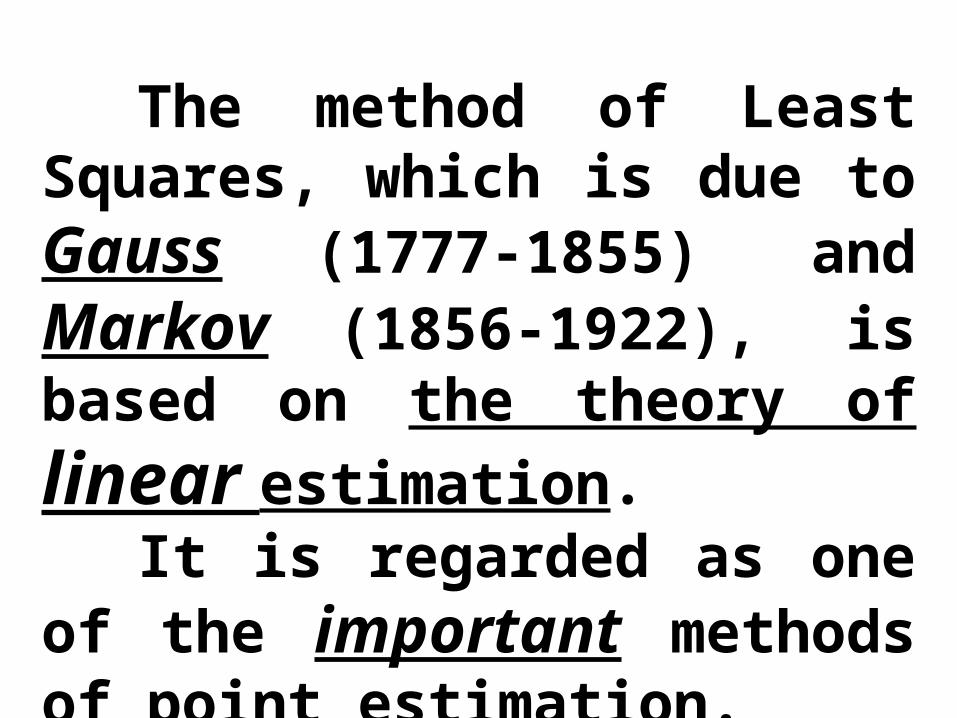
The method of Least Squares, which is due to Gauss (1777-1855) and Markov (1856-1922), is based on the theory of linear estimation.
It is regarded as one of the important methods of point estimation.
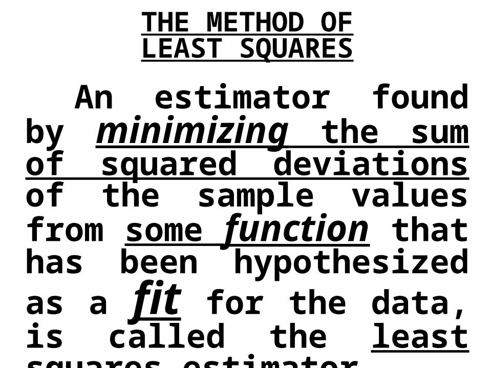
THE METHOD OFLEAST SQUARES
An estimator found by minimizing the sum of squared deviations of the sample values from some function that has been hypothesized as a fit for the data, is called the least squares estimator.
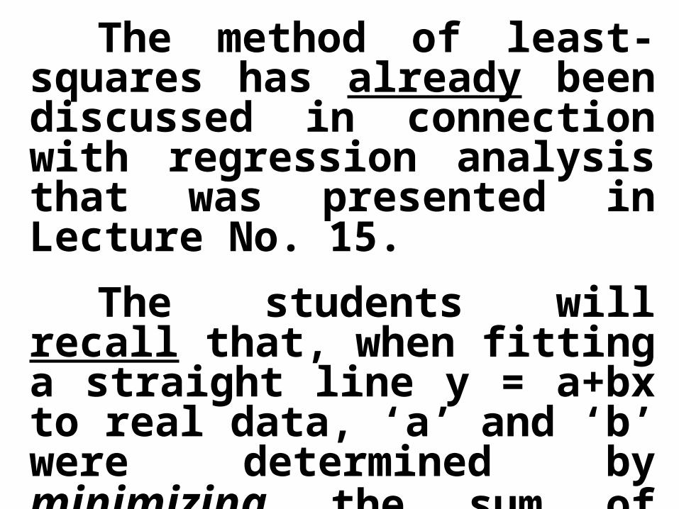
The method of least-squares has already been discussed in connection with regression analysis that was presented in Lecture No. 15.
The students will recall that, when fitting a straight line y = a+bx to real data, ‘a’ and ‘b’ were determined by minimizing the sum of squared deviations between the fitted line and the data-points.
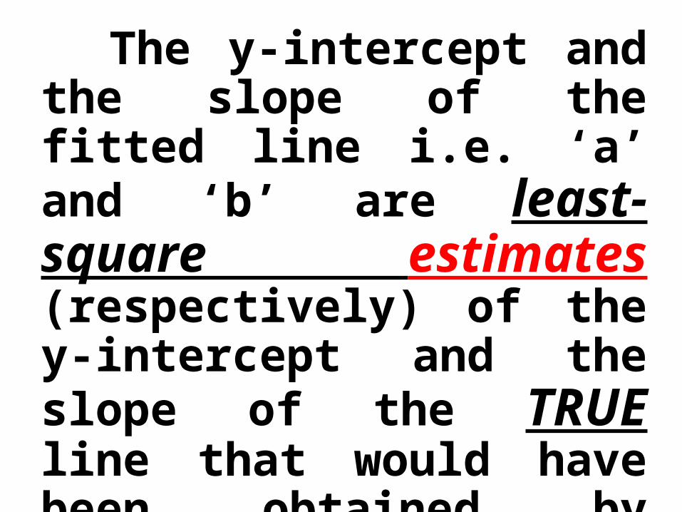
The y-intercept and the slope of the fitted line i.e. ‘a’ and ‘b’ are least-square estimates (respectively) of the y-intercept and the slope of the TRUE line that would have been obtained by considering the entire population of data-points, and not just a sample.
Next, we consider the Method of Maximum Likelihood:
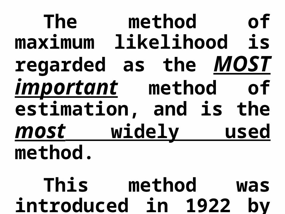
The method of maximum likelihood is regarded as the MOST important method of estimation, and is the most widely used method.
This method was introduced in 1922 by Sir Ronald A. Fisher (1890-1962).
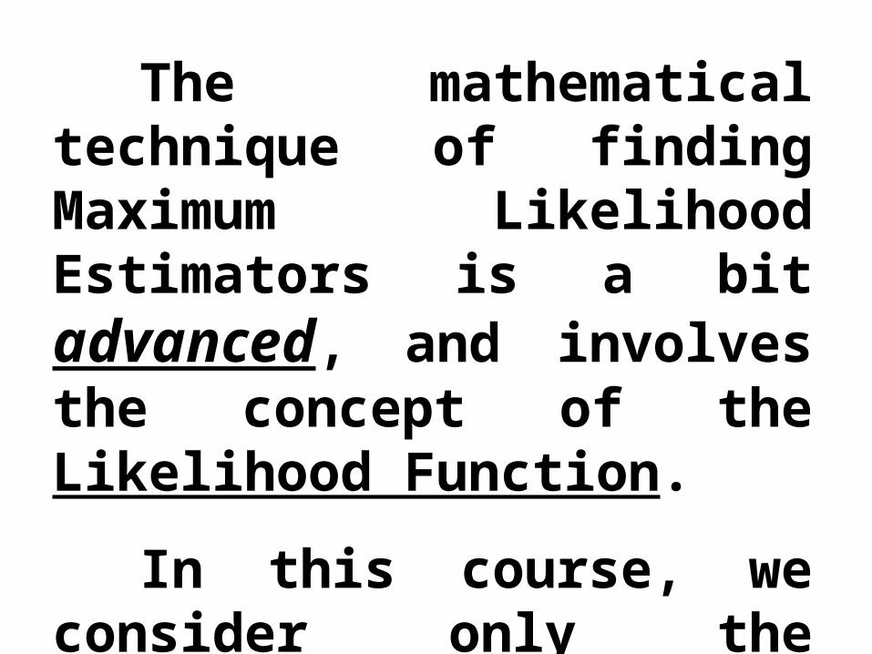
The mathematical technique of finding Maximum Likelihood Estimators is a bit advanced, and involves the concept of the Likelihood Function.
In this course, we consider only the overall logic of this method:
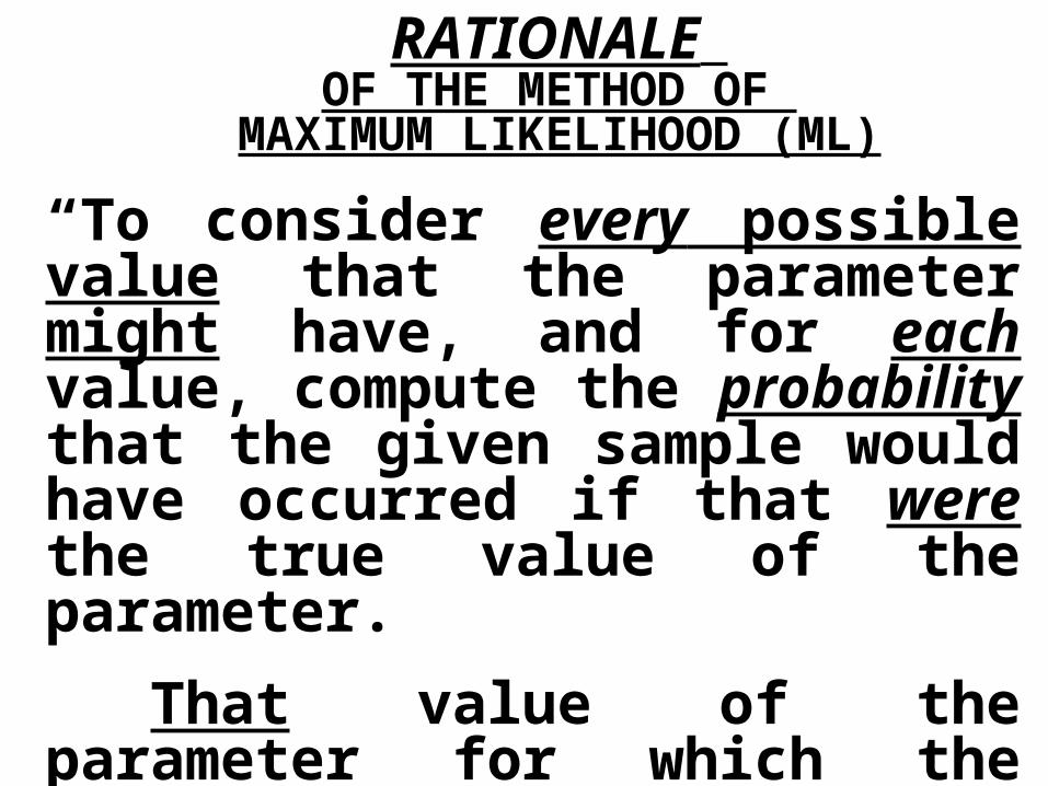
RATIONALE OF THE METHOD OF
MAXIMUM LIKELIHOOD (ML)
“To consider every possible value that the parameter might have, and for each value, compute the probability that the given sample would have occurred if that were the true value of the parameter.
That value of the parameter for which the probability of a given sample is greatest, is chosen as an estimate.”
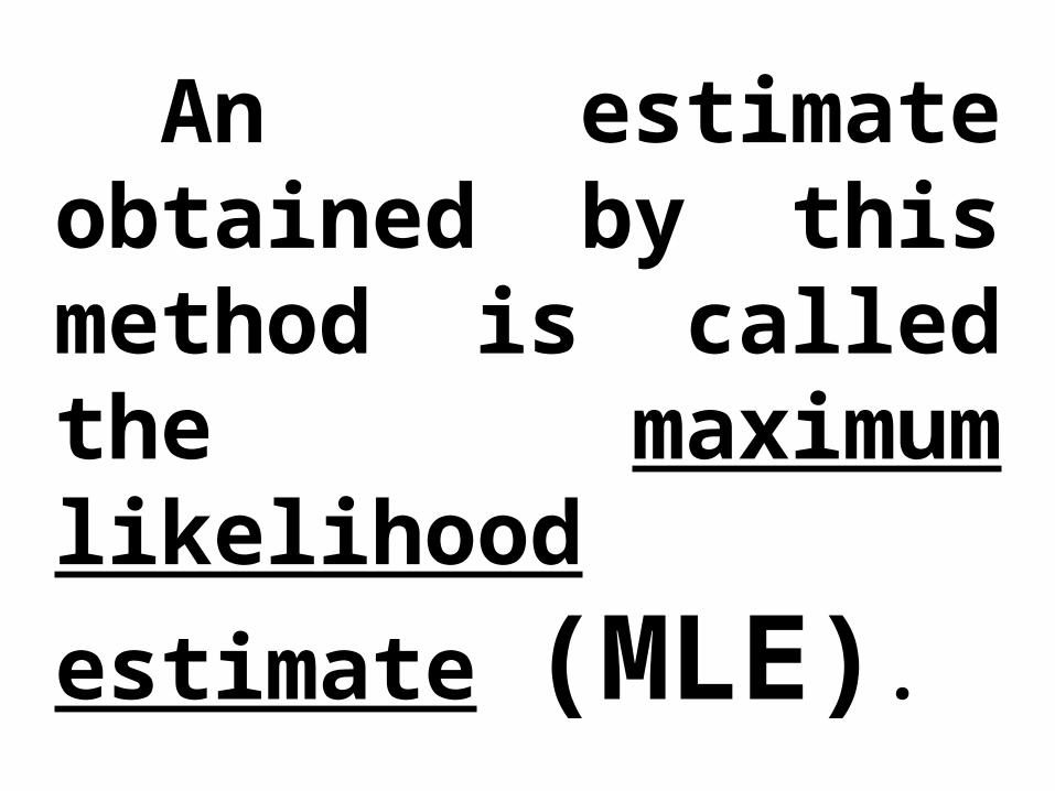
An estimate obtained by this method is called the maximum likelihood estimate (MLE).
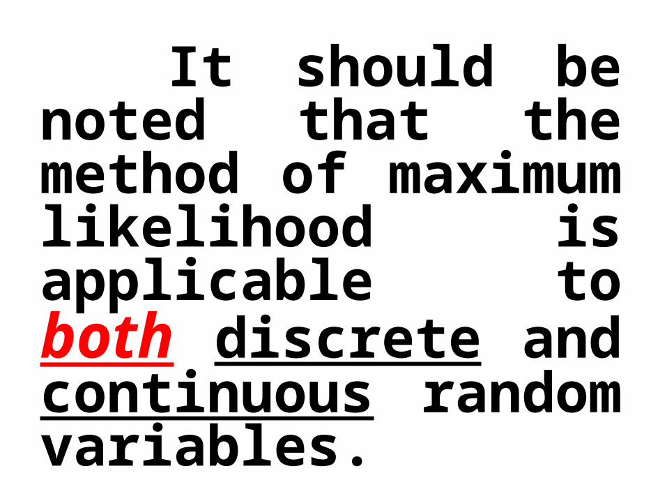
It should be noted that the method of maximum likelihood is applicable to both discrete and continuous random variables.

Let us consider a few examples:
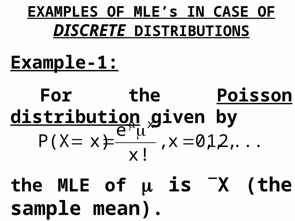
EXAMPLES OF MLE’s IN CASE OF DISCRETE DISTRIBUTIONS
Example-1:
For the Poisson distribution given by
the MLE of is X (the sample mean).
......,,2,1,0x,!x
e x) P(Xx-
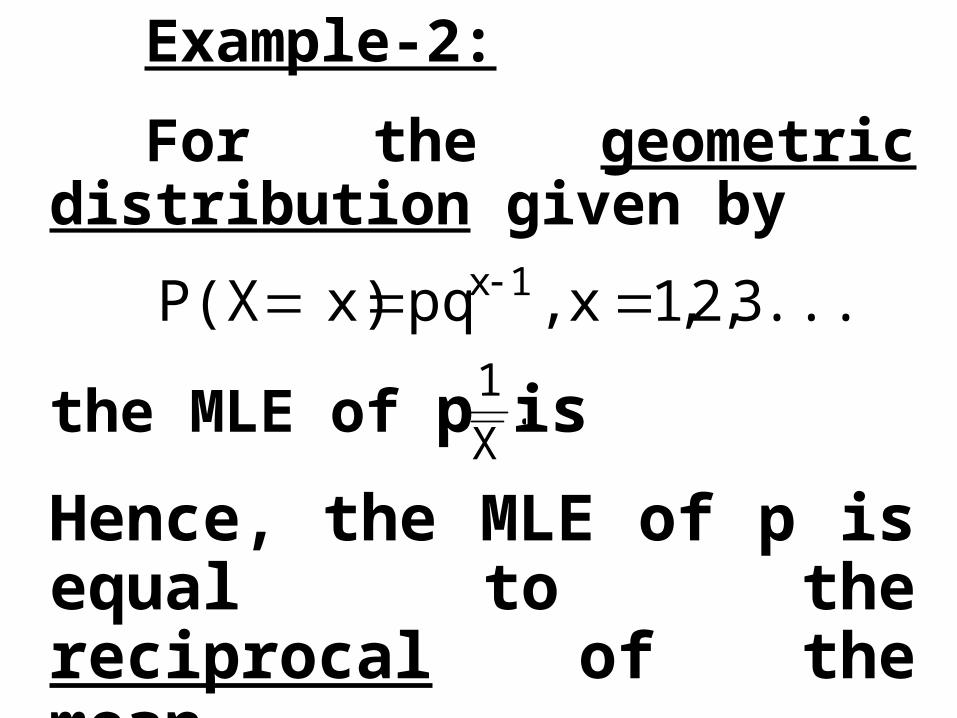
Example-2:
For the geometric distribution given by
the MLE of p is
Hence, the MLE of p is equal to the reciprocal of the mean.
......,3,2,1x,pq x) P(X 1x
.X1
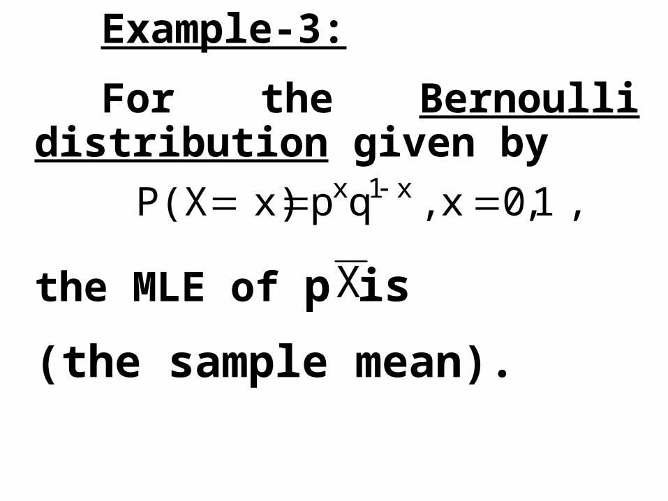
Example-3:
For the Bernoulli distribution given by
the MLE of p is
(the sample mean).
,1,0x,qp x) P(X x1x
X
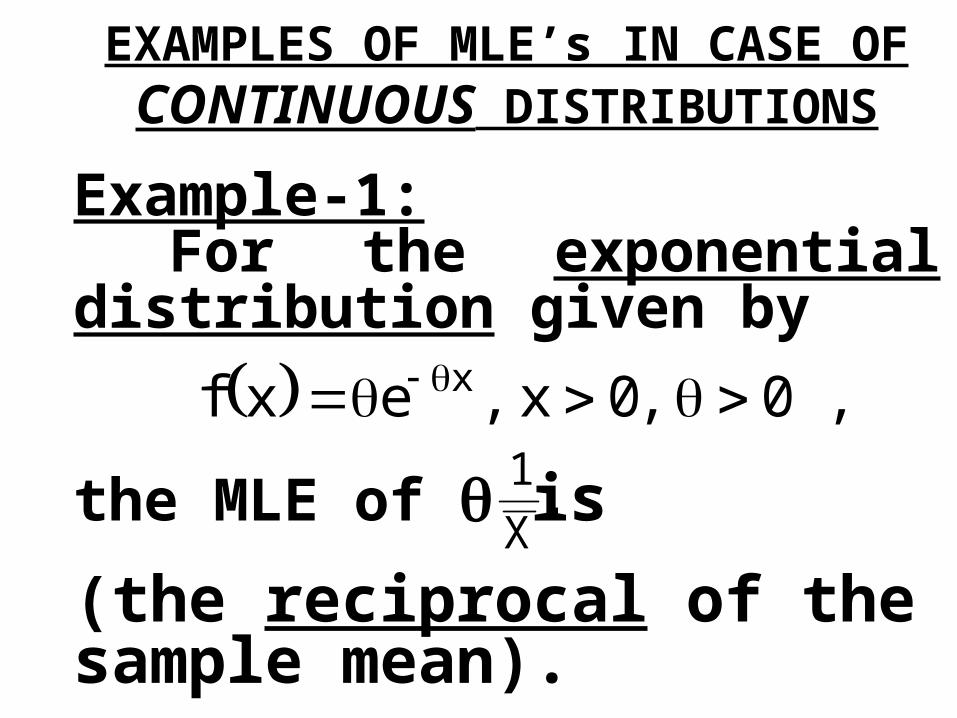
EXAMPLES OF MLE’s IN CASE OF CONTINUOUS DISTRIBUTIONS
Example-1:For the exponential
distribution given by
the MLE of is(the reciprocal of the sample mean).
,0,0x,exf x
.X1
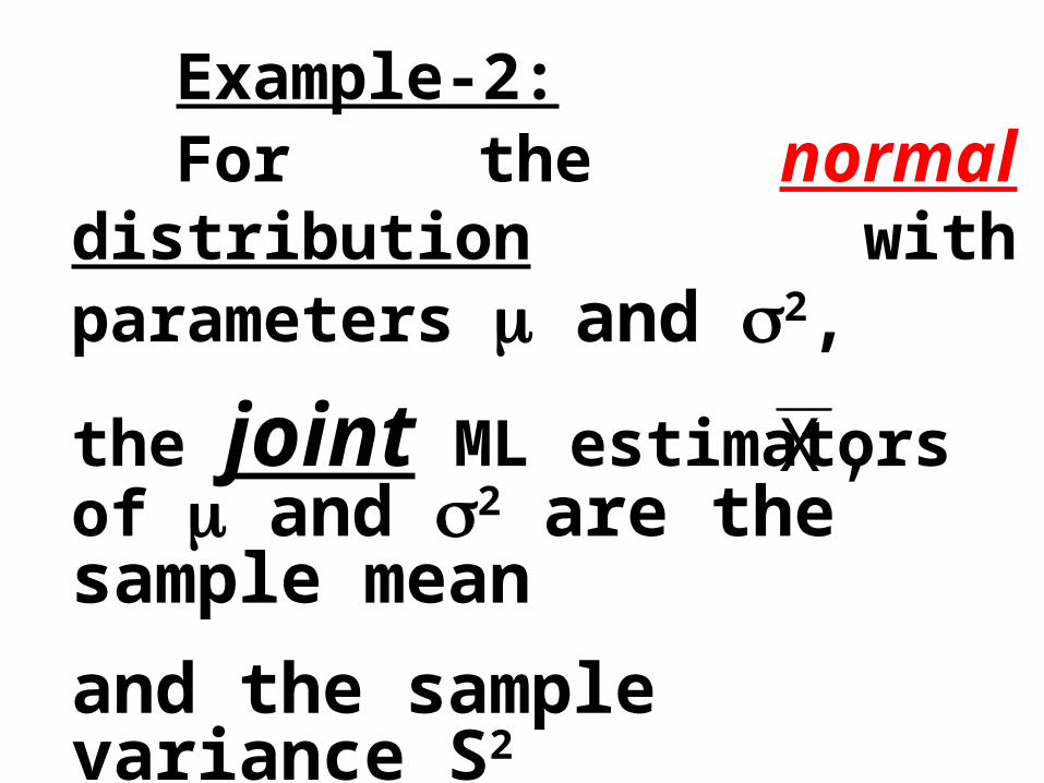
Example-2:For the normal distribution
with parameters and 2,
the joint ML estimators of and 2 are the sample mean and the sample variance S2
(which is not an unbiasedestimator of 2).
,X
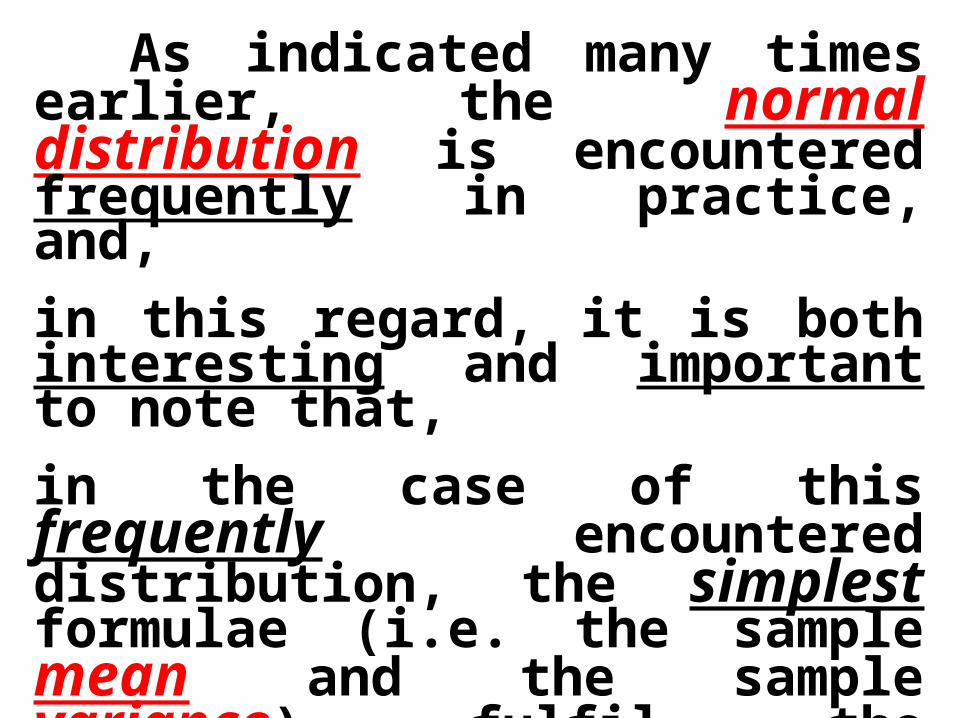
As indicated many times earlier, the normal distribution is encountered frequently in practice, and, in this regard, it is both interesting and important to note that, in the case of this frequently encountered distribution, the simplest formulae (i.e. the sample mean and the sample variance) fulfil the criteria of the relatively advanced method of maximum likelihood estimation !
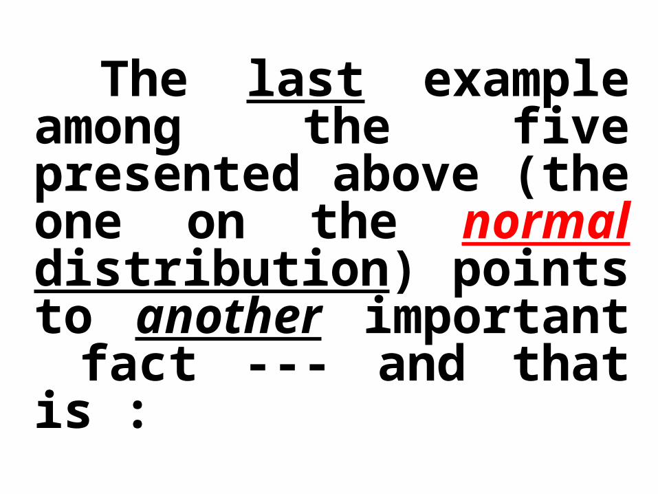
The last example among the five presented above (the one on the normal distribution) points to another important fact --- and that is :
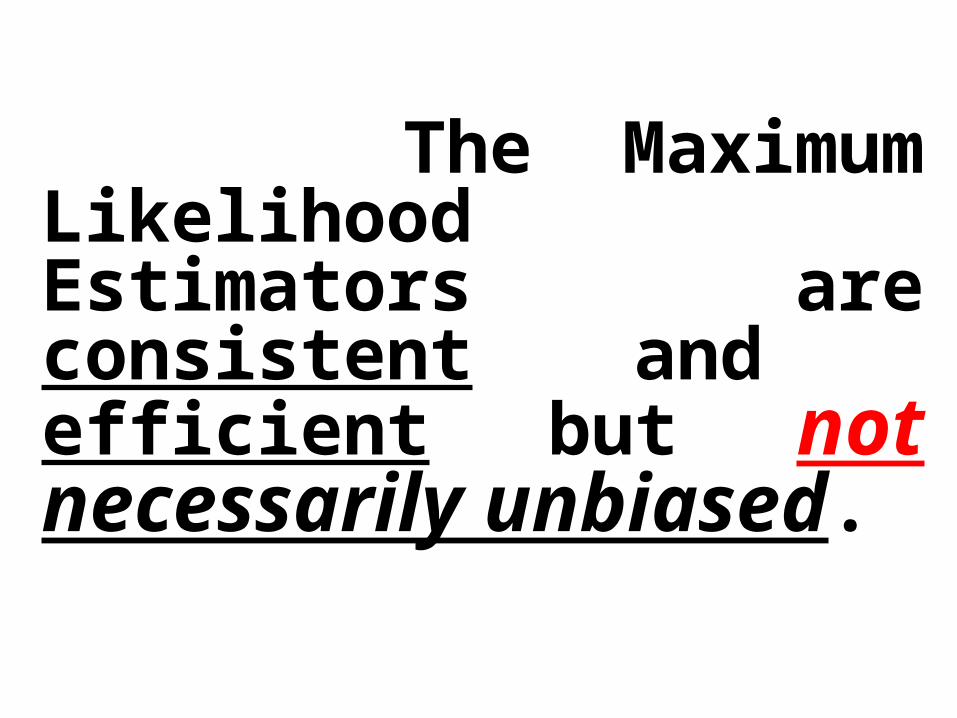
The Maximum Likelihood Estimators are consistent and efficient but not necessarily unbiased.
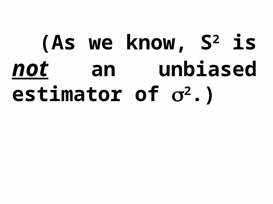
(As we know, S2 is not an unbiased estimator of 2.)

Let us apply this concept to a real-life example:
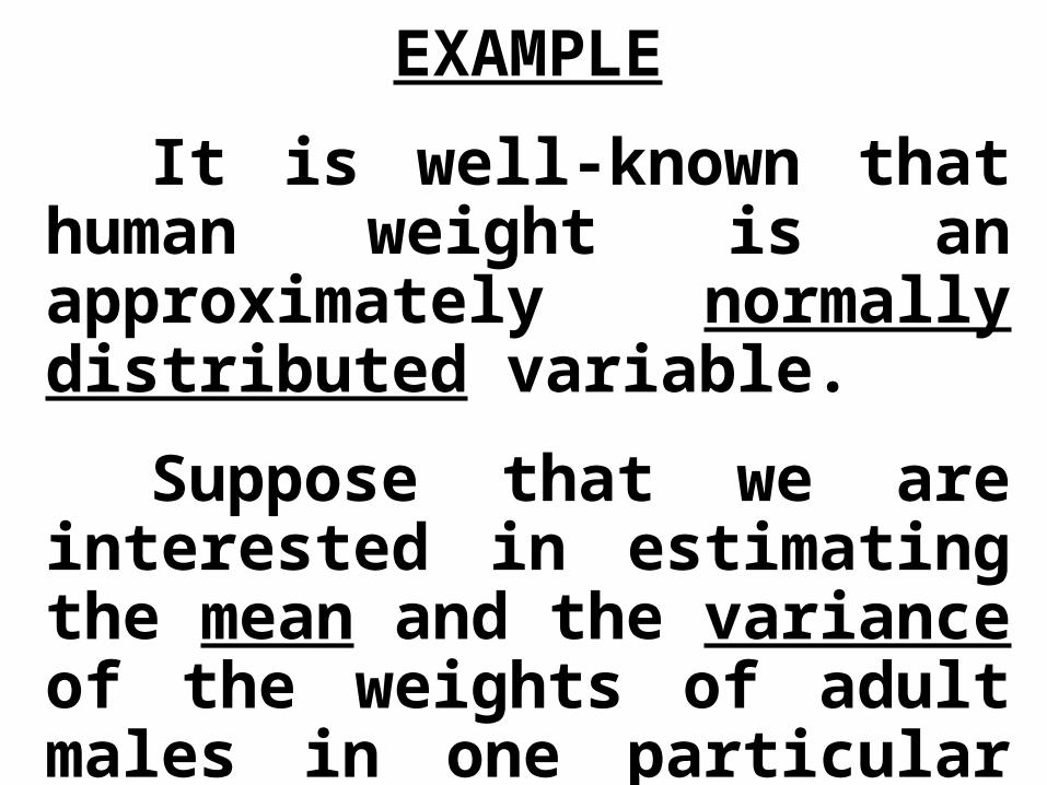
EXAMPLE
It is well-known that human weight is an approximately normally distributed variable.
Suppose that we are interested in estimating the mean and the variance of the weights of adult males in one particular province of a country.
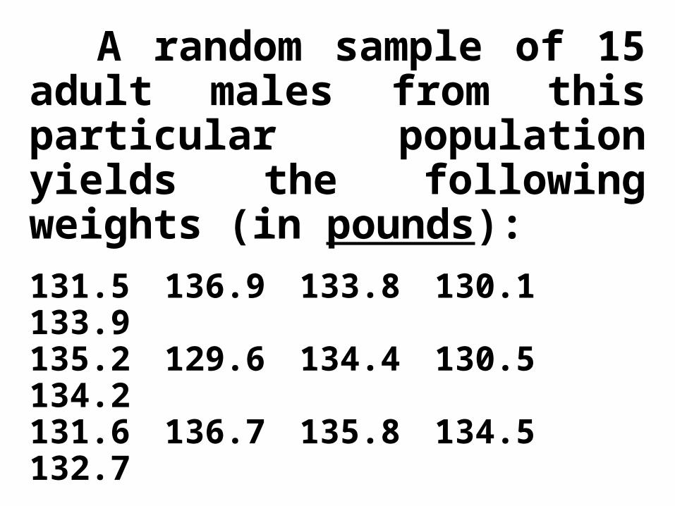
A random sample of 15 adult males from this particular population yields the following weights (in pounds):131.5 136.9 133.8 130.1 133.9135.2 129.6 134.4 130.5 134.2131.6 136.7 135.8 134.5 132.7
Find the maximum likelihood estimates for 1 = and 2 = 2.
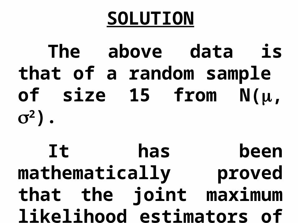
SOLUTION
The above data is that of a random sample of size 15 from N(, 2).
It has been mathematically proved that the joint maximum likelihood estimators of and 2 areX and S2.
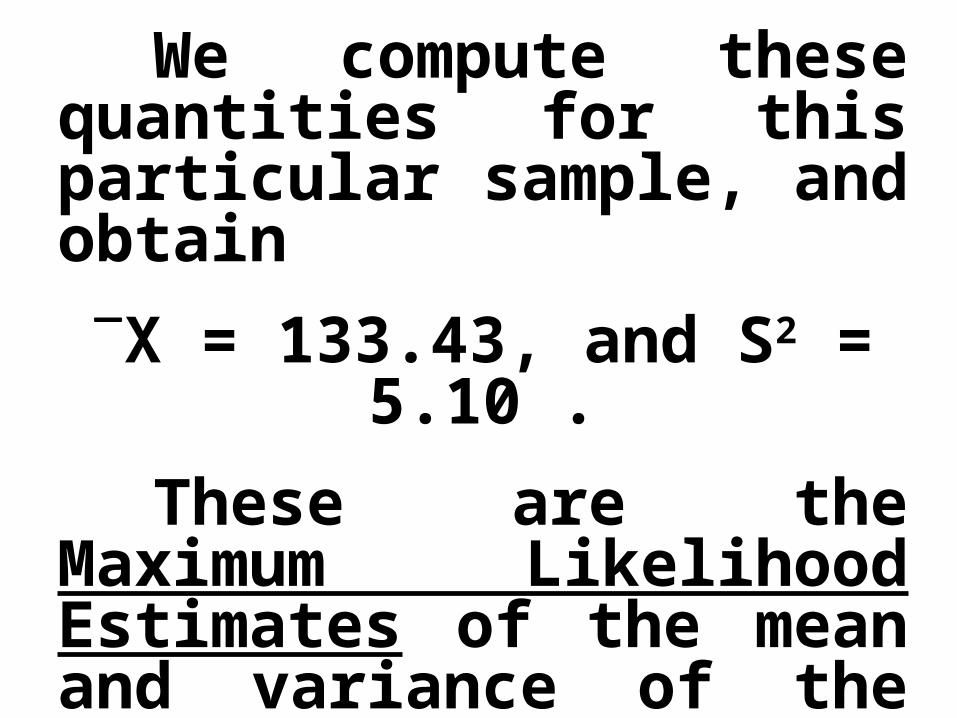
We compute these quantities for this particular sample, and obtain
X = 133.43, and S2 = 5.10 .These are the Maximum
Likelihood Estimates of the mean and variance of the population of weights in this particular example.
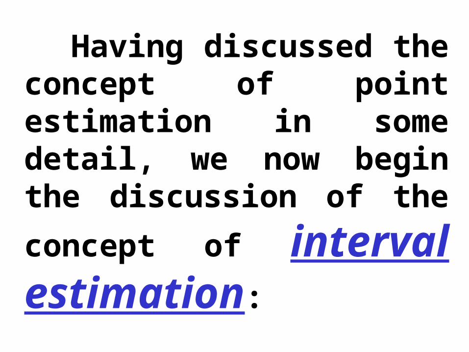
Having discussed the concept of point estimation in some detail, we now begin the discussion of the concept of interval estimation:
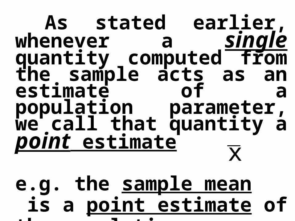
As stated earlier, whenever a single quantity computed from the sample acts as an estimate of a population parameter, we call that quantity a point estimate
e.g. the sample mean is a point estimate of the population mean .
x
The limitation of point estimation is that we have no way of ascertaining how close our point estimate is to the true value (the parameter).
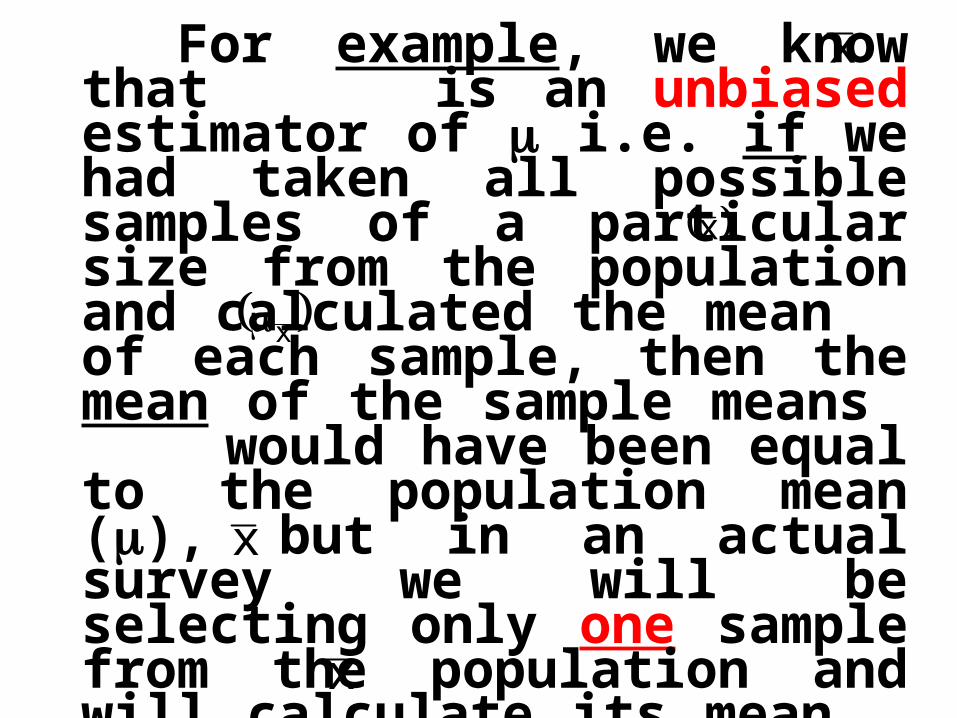
For example, we know that is an unbiased estimator of i.e. if we had taken all possible samples of a particular size from the population and calculated the mean of each sample, then the mean of the sample means would have been equal to the population mean (), but in an actual survey we will be selecting only one sample from the population and will calculate its mean .
We will have no way of ascertaining how close this particular is to .
x
x
x
x
x
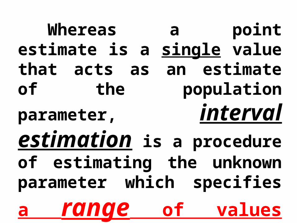
Whereas a point estimate is a single value that acts as an estimate of the population parameter, interval estimation is a procedure of estimating the unknown
parameter which specifies a range of values within which the parameter is expected to lie.
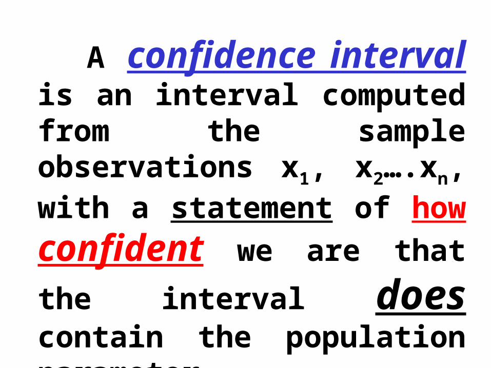
A confidence interval is an interval computed from the sample observations x1, x2….xn, with a statement of how confident we are that the interval does contain the population parameter.

We develop the concept of interval estimation with the help of the example of the Ministry of Transport test to which all cars, irrespective of age, have to be submitted :

EXAMPLELet us examine the case of an
annual Ministry of Transport test to which all cars, irrespective of age, have to be submitted.
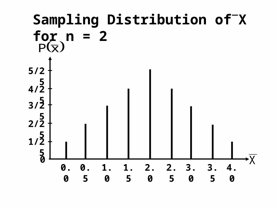
The test looks for faulty breaks, steering, lights and suspension, and it is discovered after the first year that approximately the same number of cars have 0, 1, 2, 3, or 4 faults.
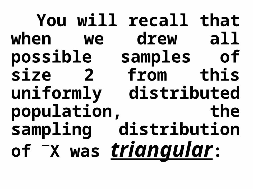
You will recall that when we drew all possible samples of size 2 from this uniformly distributed population, the sampling distribution of X was triangular:
1/25
00.5 1.0 1.5 2.0 2.5 3.0 3.5 4.0
X
2/25
3/25
4/25
5/25
0.0
xP
Sampling Distribution ofX for n = 2
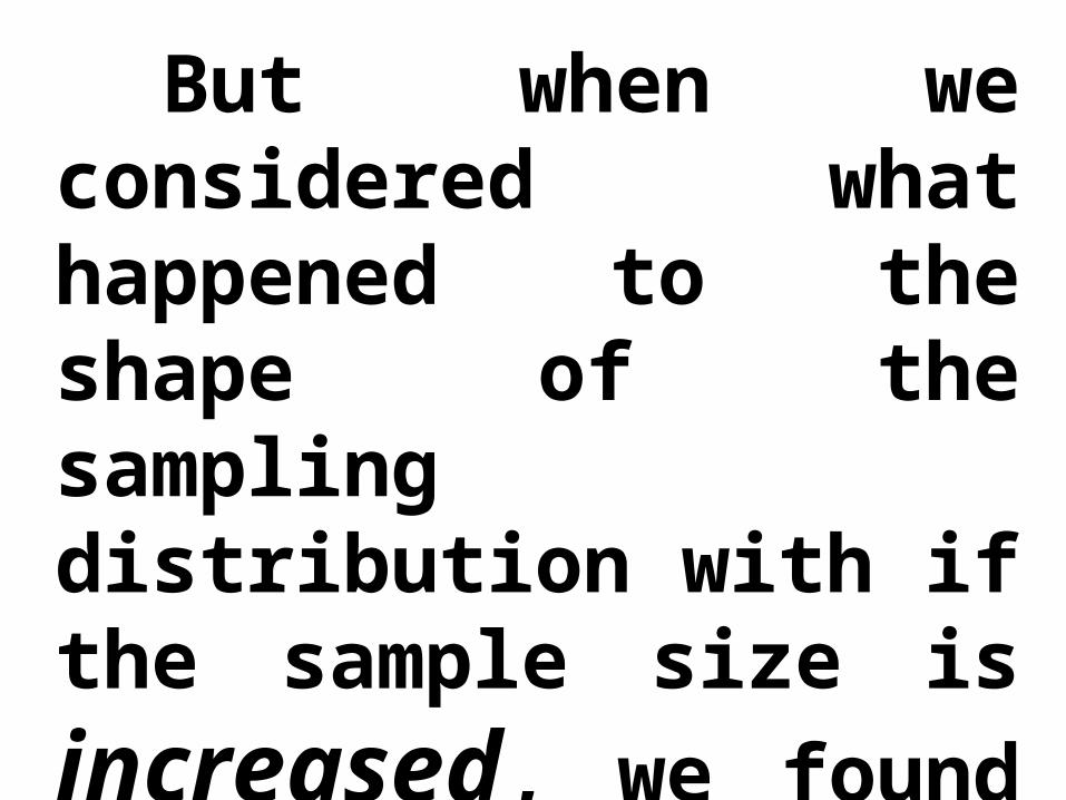
But when we considered what happened to the shape of the sampling distribution with if the sample size is increased, we found that it was somewhat like a normal distribution:
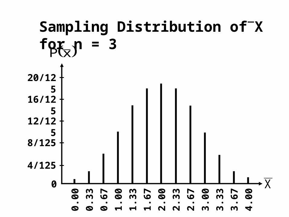
4/125
0 X
0.00
xP
0.33
0.67
1.00
1.33
1.67
2.00
2.33
2.67
3.00
3.33
3.67
4.00
8/125
12/125
16/125
20/125
Sampling Distribution ofX for n = 3
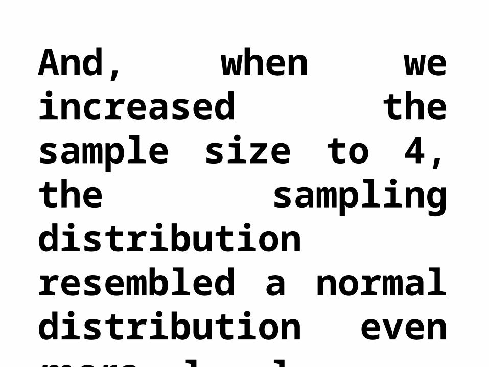
And, when we increased the sample size to 4, the sampling distribution resembled a normal distribution even more closely :
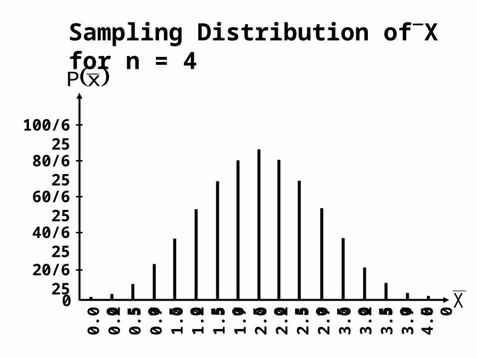
Sampling Distribution ofX for n = 4
20/625
0 X
xP
40/625
60/625
80/625
100/625
0.75
0.50
0.25
0.00
1.75
1.50
1.25
1.00
2.75
2.50
2.25
2.00
3.75
3.50
3.25
3.00
4.00
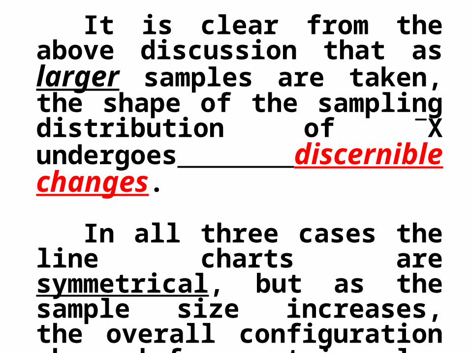
It is clear from the above discussion that as larger samples are taken, the shape of the sampling distribution of X undergoes discernible changes.
In all three cases the line charts are symmetrical, but as the sample size increases, the overall configuration changed from a triangular distribution to a bell-shaped distribution.
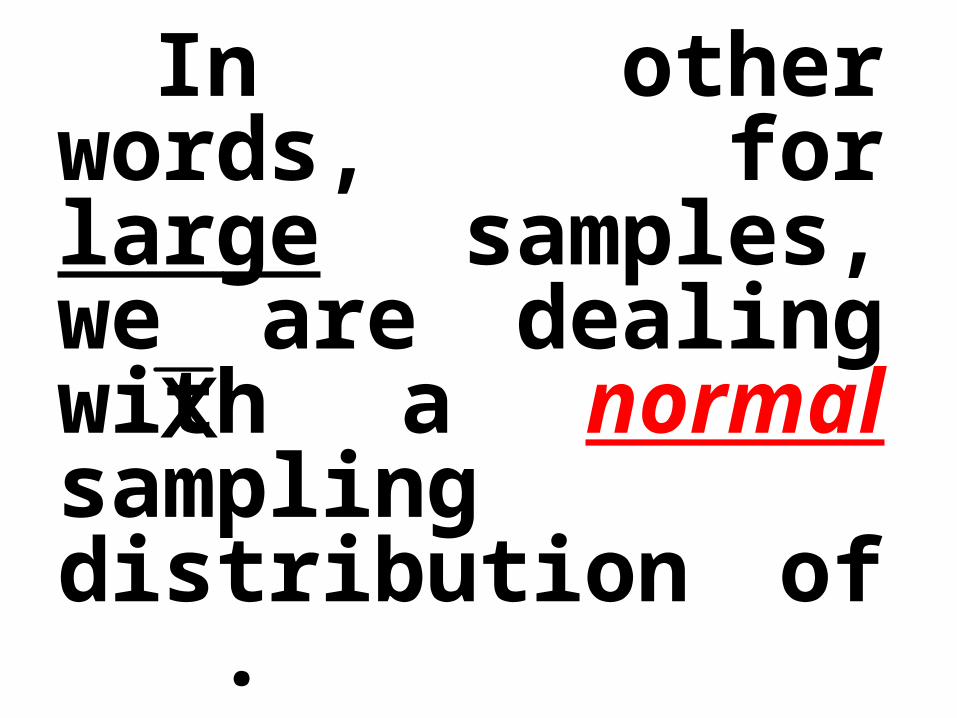
In other words, for large samples, we are dealing with a normal sampling distribution of .
In other words:
x
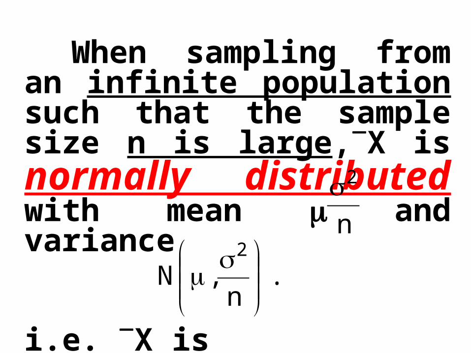
When sampling from an infinite population such that the sample size n is large,X is normally distributed with mean and variance
i.e. X is
n
2
.n
,N2
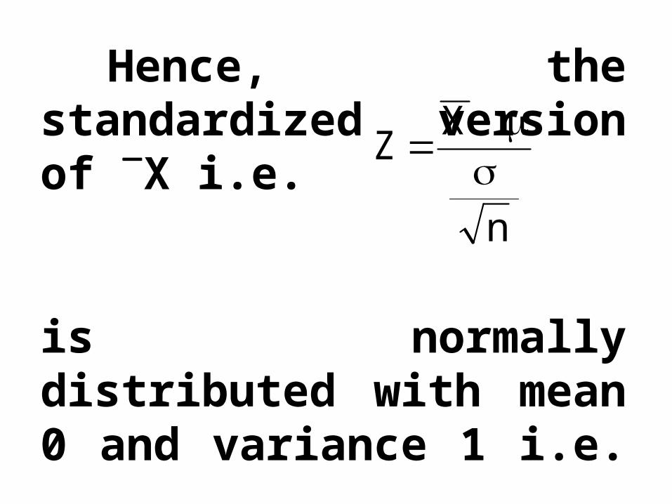
Hence, the standardized version of X i.e.
is normally distributed with mean 0 and variance 1 i.e.
Z is N(0, 1).
n
XZ

Now, for the standard normal distribution, we have:
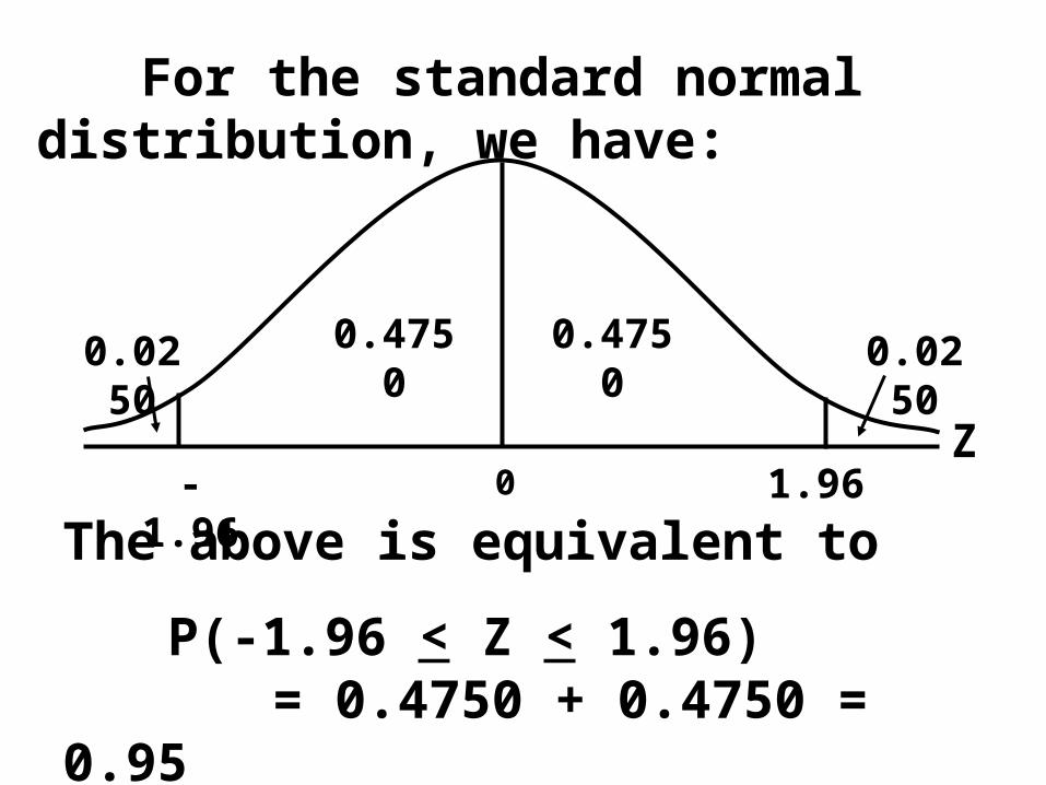
1.960-1.96
0.47500.4750 0.02500.0250
Z
For the standard normal distribution, we have:
The above is equivalent to
P(-1.96 < Z < 1.96)= 0.4750 + 0.4750 = 0.95
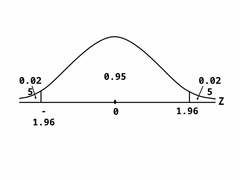
1.960-1.96
0.95 0.0250.025
Z
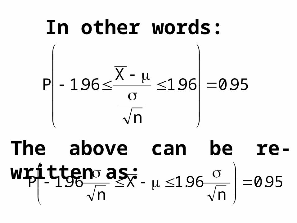
In other words:
95.096.1
n
X96.1P
The above can be re-written as:95.0
n96.1X
n96.1P
95.0n
96.1Xn
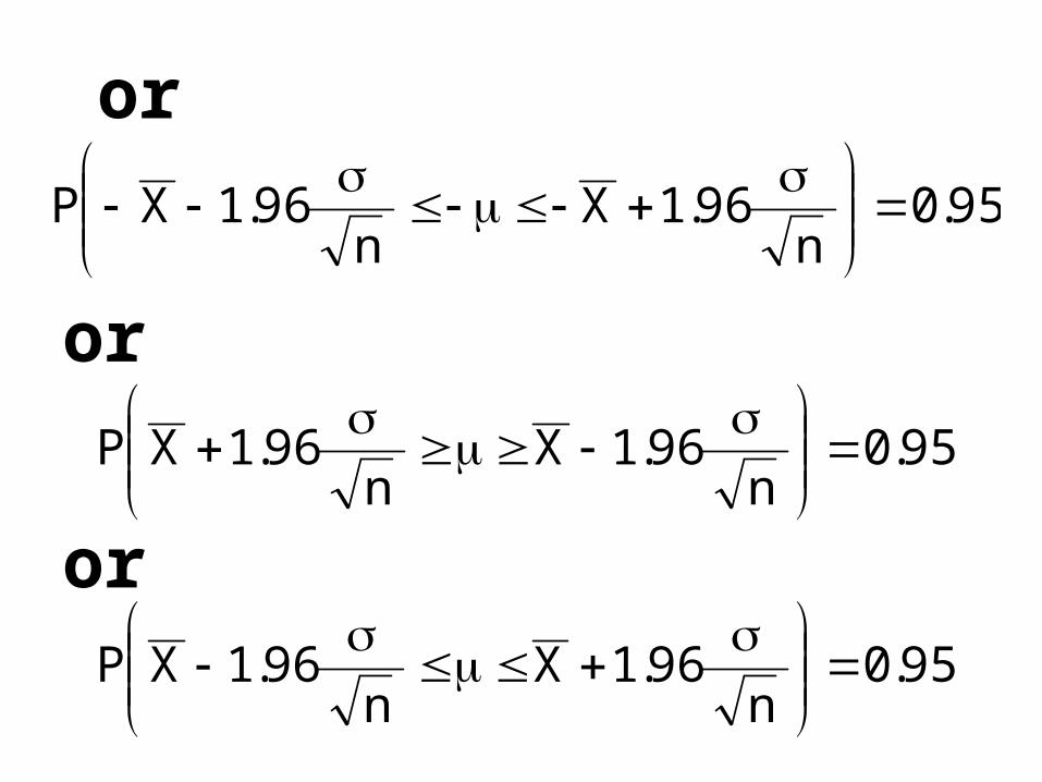
96.1XP
or
or95.0
n96.1X
n96.1XP
95.0n
96.1Xn
96.1XP
or
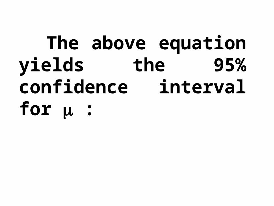
The above equation yields the 95% confidence interval for :
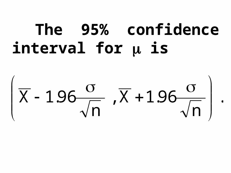
The 95% confidence interval for is
.n
96.1X,n
96.1X
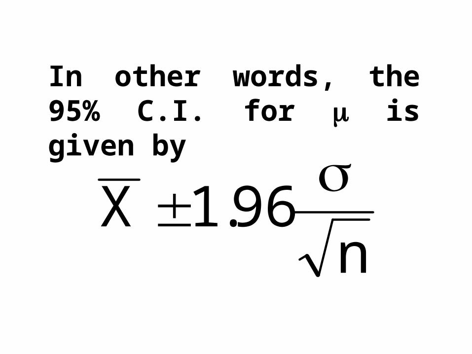
In other words, the 95% C.I. for is given by
n96.1X
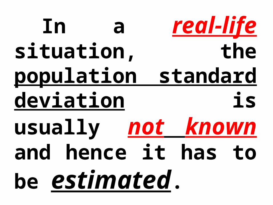
In a real-life situation, the population standard deviation is usually not known and hence it has to be estimated.
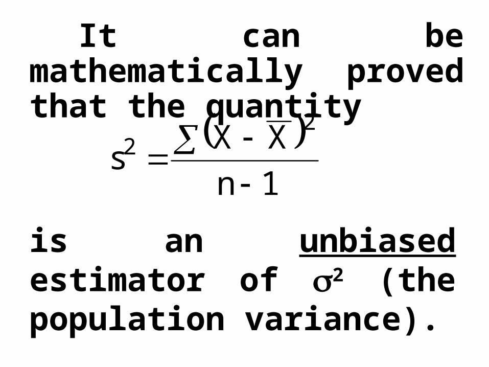
1nXXs
22
It can be mathematically proved that the quantity
is an unbiased estimator of 2 (the population variance).
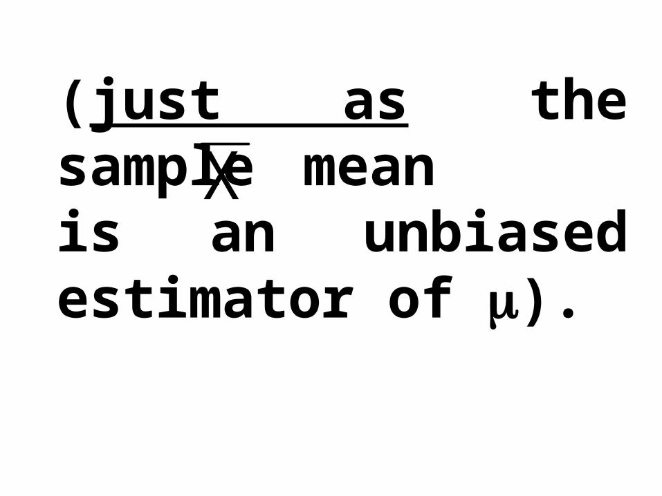
(just as the sample mean is an unbiased estimator of ).
X
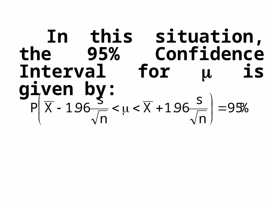
In this situation, the 95% Confidence Interval for is given by:
%95ns96.1X
ns96.1XP
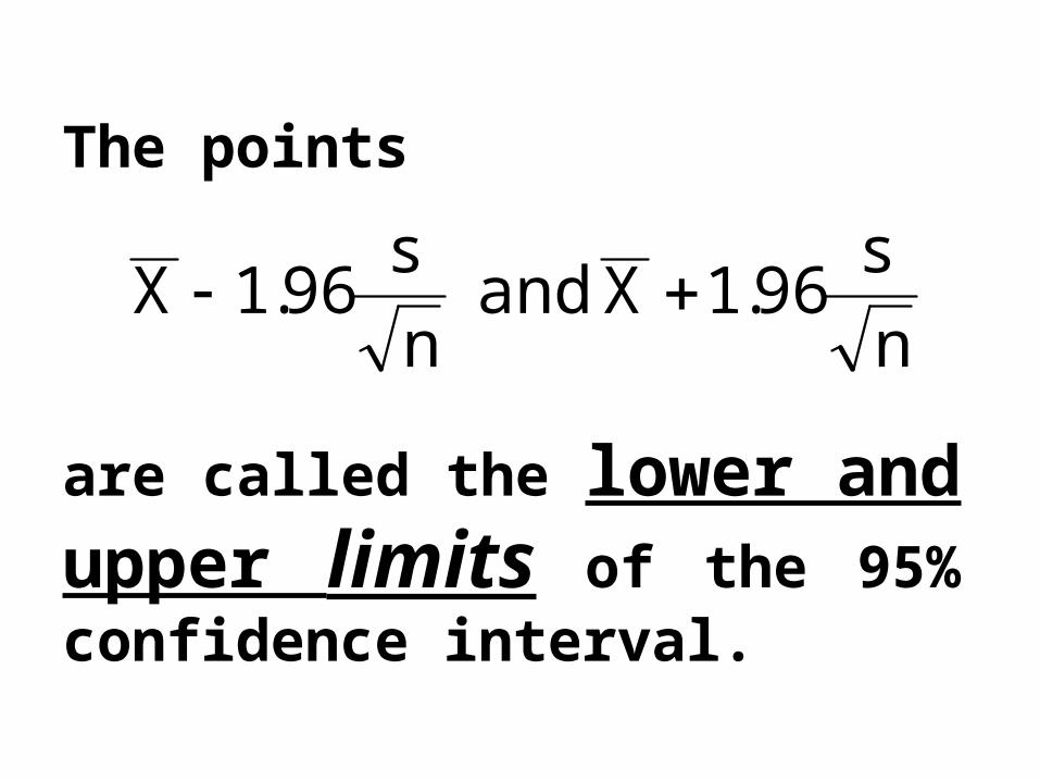
The points
are called the lower and upper limits of the 95% confidence interval.
ns96.1Xand
ns96.1X
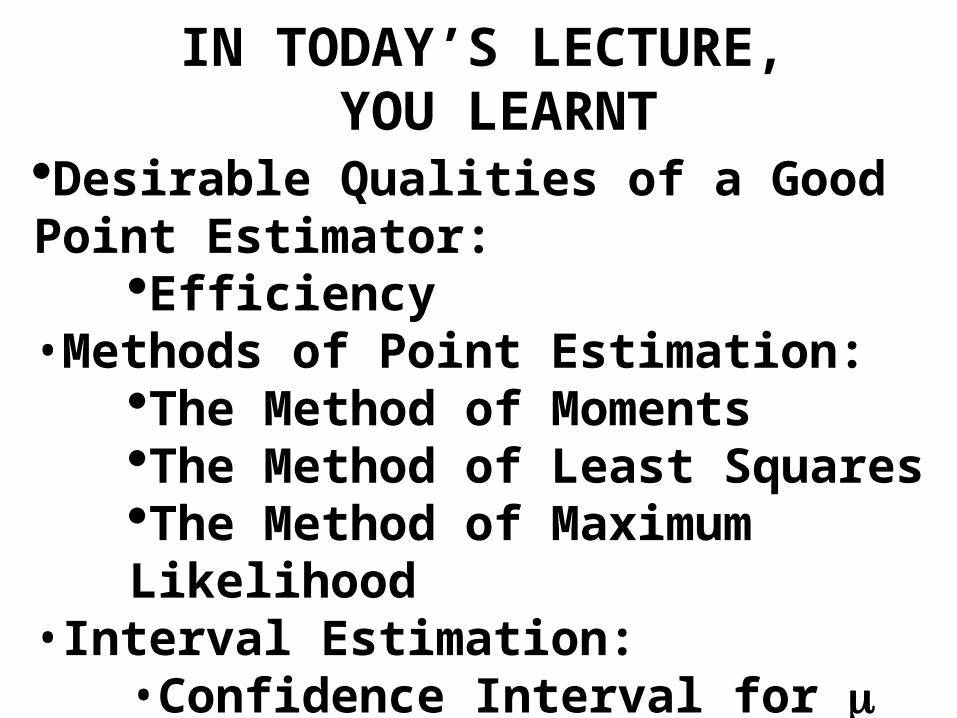
IN TODAY’S LECTURE, YOU LEARNT
Desirable Qualities of a Good Point Estimator:
Efficiency•Methods of Point Estimation:
The Method of MomentsThe Method of Least SquaresThe Method of Maximum Likelihood
•Interval Estimation:•Confidence Interval for
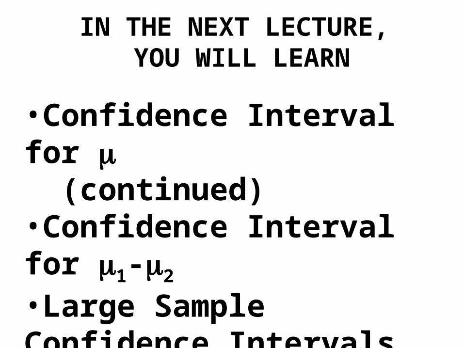
IN THE NEXT LECTURE, YOU WILL LEARN
•Confidence Interval for (continued)•Confidence Interval for 1-2
•Large Sample Confidence Intervals for p and p1-p2
•Determination of Sample Size


