23

CHAPTER II

OVERVIEW OF STABILITY ANALYSIS AND DESIGN METHODS IN AISC (2010)

2.1 Background

Chapter C of AISC (2010), Design for Stability, states that any analysis and

design procedure that addresses the following effects on the overall stability of the

structure and its elements is permitted:

1. Flexural, axial and shear deformations (in members, connections and other

components), and all other deformations that contribute to displacements of the

structure,

2. Reduction in stiffness (and corresponding increases in deformations) due to residual

stresses and material yielding,

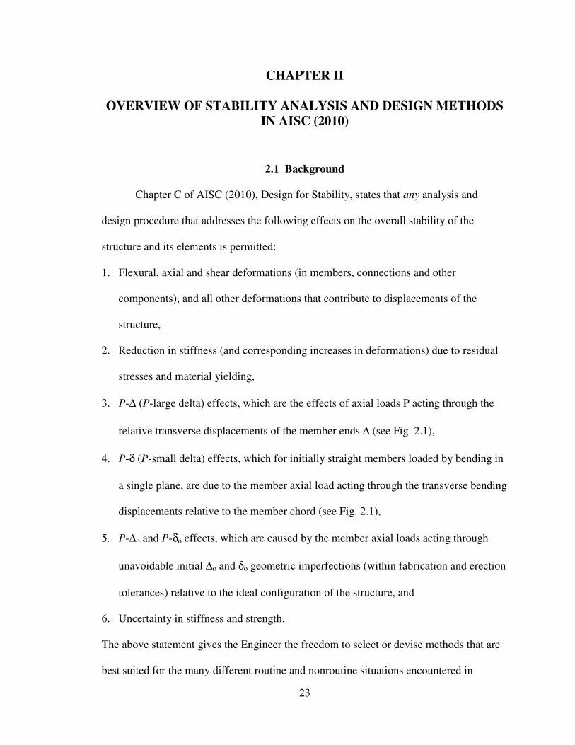
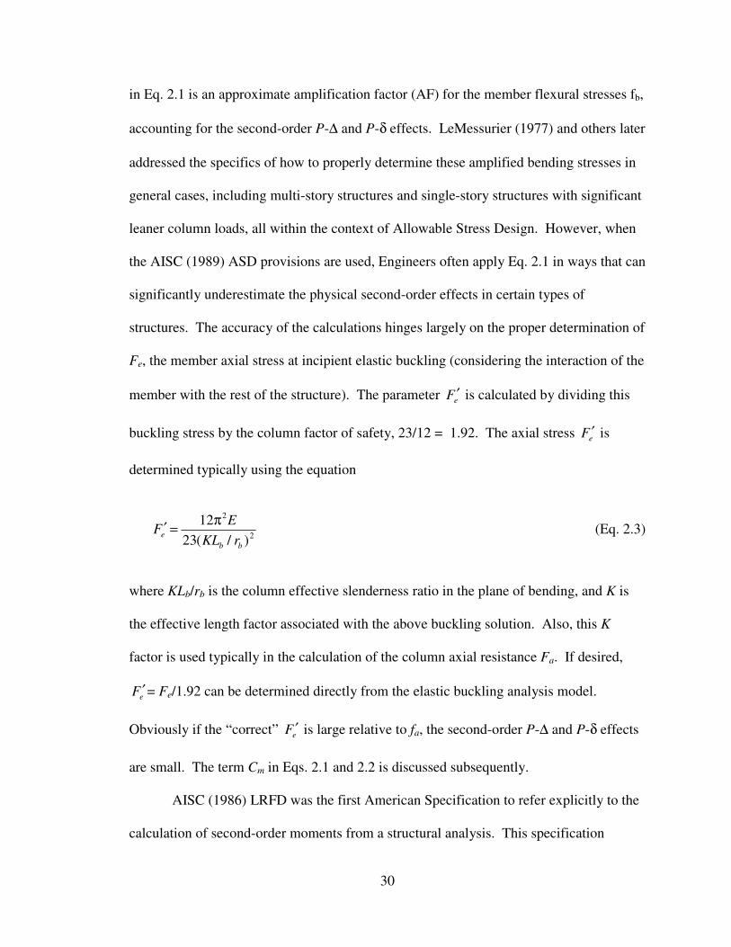
3. P-Δ (P-large delta) effects, which are the effects of axial loads P acting through the

relative transverse displacements of the member ends Δ (see Fig. 2.1),

4. P-δ (P-small delta) effects, which for initially straight members loaded by bending in

a single plane, are due to the member axial load acting through the transverse bending

displacements relative to the member chord (see Fig. 2.1),

5. P-Δo and P-δo effects, which are caused by the member axial loads acting through

unavoidable initial Δo and δo geometric imperfections (within fabrication and erection

tolerances) relative to the ideal configuration of the structure, and

6. Uncertainty in stiffness and strength.

The above statement gives the Engineer the freedom to select or devise methods that are

best suited for the many different routine and nonroutine situations encountered in

24

practice. It allows for innovation within the constraints of the proper consideration of the

physical effects that influence the structural response.

Figure 2.1. Second-order P-Δ and P-δ effects.

Since the P-Δ and P-δ effects are central components of the frame stability

behavior, it is useful to elaborate on their definitions. As illustrated in Figure 2.1, any

relative transverse displacement Δ between a member’s ends produces a couple of P

times Δ, where P is the axial force transmitted by the member. This couple must be

resisted by the structure. In typical tiered building systems, the predominant P-Δ effects

come from the vertical columns. However, clear-span gable frames also have a P-Δ

effect associated with the axial thrust in the rafters and the relative transverse

displacement between the ends of the rafter segments, as shown in Figure 2.2. In certain

types of structures, e.g., some types of modular frames, the predominant P-Δ effects

come from simply-connected gravity columns (leaner columns), which depend on the

lateral load resisting system for their lateral stability. Figure 2.3 gives a simple

25

illustration of this behavior. Under a sidesway displacement of the structure Δ, a lateral

force equal to PΔ/L is required to maintain equilibrium of the leaner column in the

deflected configuration. This lateral force must be resisted by the structure.

�

Figure 2.2. P-Δ effects in a rafter segment of a gable frame.

Figure 2.3. Illustration of P-Δ effects from a gravity (leaner) column.

Members that have small transverse displacements relative to their rotated chord

and/or small axial forces have small P-δ effects. This includes leaner columns, which are

commonly idealized as straight pin-ended struts and therefore have zero δ and zero P-δ

effects, as well as stiff columns that deflect in sidesway mainly due to end rotation of the

26

adjacent beams (see Figure 2.4). However, members such as that shown in Figure 2.1

must resist additional moments of P times δ at the various cross-sections along their

lengths. These P-δ moments increase the member deformations, and therefore they

reduce the net member stiffnesses and increase the net sidesway displacements Δ.

Interestingly, if the structure is subdivided into a large number of short-length elements,

the representation of the P-Δ effect in each element is sufficient to capture both the

overall member P-Δ and the internal member P-δ effects. Figure 2.2 is to some extent

indicative of this attribute.

Figure 2.4. Illustration of deformed geometry resulting in small P-δ effects.

Guney and White (2007) study the number of elements required per member for

P-large delta only analysis procedures to ensure less than 5 % error in the nodal

displacements and less than 3 % error in the maximum internal moments for second-

order elastic analysis of prismatic members with a wide range of loadings and end

conditions. They also address the number of elements required to ensure less than 2 %

27

error in eigenvalue buckling analysis solutions. Based on the research by Guney and

White (2007), the AISC Design Guide 25 provides tables showing the required number of

elements to achieve the desired analysis accuracy for a given calculated αPr /PeL or αPr

/ eLP value for sway columns with simply-supported bases, sway columns with top and

bottom rotational restraints, and rafters and non-sway columns, where PeL is the member

elastic buckling load based on the idealized simply-supported end conditions and nominal

elastic stiffness and eLP is the member elastic buckling load based on the idealized

simply-supported end conditions and reduced elastic stiffness specified by the direct

analysis method. For example, at αPr /PeL = 0.15, three elements are required for a sway

column to ensure less than 5 % error in the nodal displacements and less than 3 % error in

the maximum internal moments. In general, P-large delta only analysis procedures can

adequately capture internal member P-δ effects when the subdivisions of members

achieve αPr < 0.02Pe� or αPr < 0.02 �eP , where Pe� is the element elastic buckling load

based on idealized simply-supported end conditions and nominal stiffness and �eP element

elastic buckling load based on idealized simply-supported end conditions and reduced

stiffness specified in the direct analysis method. Second-order analysis methods that

directly include both P-Δ and P-δ effects at the element level generally provide better

accuracy than P-large delta analysis procedures.

In tapered-web and general nonprismatic members, the centroidal axis is not

straight, thus causing additional moments of P times y, where y is the shift in the

centroidal axis relative to a straight chord between the cross-section centroids at the

member ends (see Figure 2.5). This important effect is incorporated within a proper first-

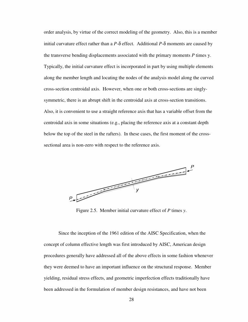
28

order analysis, by virtue of the correct modeling of the geometry. Also, this is a member

initial curvature effect rather than a P-δ effect. Additional P-δ moments are caused by

the transverse bending displacements associated with the primary moments P times y.

Typically, the initial curvature effect is incorporated in part by using multiple elements

along the member length and locating the nodes of the analysis model along the curved

cross-section centroidal axis. However, when one or both cross-sections are singly-

symmetric, there is an abrupt shift in the centroidal axis at cross-section transitions.

Also, it is convenient to use a straight reference axis that has a variable offset from the

centroidal axis in some situations (e.g., placing the reference axis at a constant depth

below the top of the steel in the rafters). In these cases, the first moment of the cross-

sectional area is non-zero with respect to the reference axis.

Figure 2.5. Member initial curvature effect of P times y.

Since the inception of the 1961 edition of the AISC Specification, when the

concept of column effective length was first introduced by AISC, American design

procedures generally have addressed all of the above effects in some fashion whenever

they were deemed to have an important influence on the structural response. Member

yielding, residual stress effects, and geometric imperfection effects traditionally have

been addressed in the formulation of member design resistances, and have not been

29

considered in the analysis except the following case. Engineers have often included a

nominal out-of-plumbness effect in the analysis of gravity load combinations, particularly

if the geometry and loading are symmetric. Strictly, this is not necessary for the in-plane

strength assessment of beam-columns in the prior AISC Specifications. However, this

practice is necessary to determine P-Δo effects on bracing forces, beam moments,

connection moments, and in-plane member moments for checking the out-of-plane

resistance of beam-columns. There also has always been implicit recognition that the

engineers can use their professional judgment to disregard specific effects (e.g., member

shear deformations, connection deformations, etc.) whenever they are deemed to be

negligible.

Furthermore, the 1961 AISC Specification, and other AISC Specifications up

until 1986, relied strictly on the structural analysis only for calculation of linear elastic

forces and moments within the idealized perfectly straight and plumb nominally elastic

structural system. The influence of second-order (P-Δ and P-δ) effects was addressed

solely by an amplifier applied discreetly to the flexural stresses from the linear elastic

analysis, via the following beam-column strength interaction equation:

0.1

1

≤

���

����

�′

−

+

be

a

bm

a

a

FF

f

fC

F

f (Eq. 2.1)

The expression

AF

F

f

C

e

a

m=

���

����

�′

−1

(Eq. 2.2)

30

in Eq. 2.1 is an approximate amplification factor (AF) for the member flexural stresses fb,

accounting for the second-order P-Δ and P-δ effects. LeMessurier (1977) and others later

addressed the specifics of how to properly determine these amplified bending stresses in

general cases, including multi-story structures and single-story structures with significant

leaner column loads, all within the context of Allowable Stress Design. However, when

the AISC (1989) ASD provisions are used, Engineers often apply Eq. 2.1 in ways that can

significantly underestimate the physical second-order effects in certain types of

structures. The accuracy of the calculations hinges largely on the proper determination of

Fe, the member axial stress at incipient elastic buckling (considering the interaction of the

member with the rest of the structure). The parameter eF ′ is calculated by dividing this

buckling stress by the column factor of safety, 23/12 = 1.92. The axial stress eF ′ is

determined typically using the equation

2

2

)/(23

12

bbe rKL

EF

π=′ (Eq. 2.3)

where KLb/rb is the column effective slenderness ratio in the plane of bending, and K is

the effective length factor associated with the above buckling solution. Also, this K

factor is used typically in the calculation of the column axial resistance Fa. If desired,

eF ′= Fe/1.92 can be determined directly from the elastic buckling analysis model.

Obviously if the “correct” eF ′ is large relative to fa, the second-order P-Δ and P-δ effects

are small. The term Cm in Eqs. 2.1 and 2.2 is discussed subsequently.

AISC (1986) LRFD was the first American Specification to refer explicitly to the

calculation of second-order moments from a structural analysis. This specification

31

introduced the following two-equation format for its primary beam-column strength

interaction curve:

0.12

≤φ

+φ nb

u

nc

u

M

M

P

P for 2.0<

φ nc

u

P

P (Eq. 2.4a)

0.19

8≤

φ+

φ nb

u

nc

u

M

M

P

P for 2.0≥

φ nc

u

P

P (Eq. 2.4b)

where Mu is defined as the maximum second-order elastic moment along the member

length. AISC (1986) states that Mu may be determined from a second-order elastic

analysis using factored loads. However it also provides an amplification factor procedure

for calculation of the second-order elastic moments from a first-order elastic analysis.

This procedure is in essence an approximate second-order analysis. The above moments

Mu are the second-order elastic moments in the idealized initially plumb and straight,

nominally elastic structure.

In all the AISC Specifications from AISC (1961) through AISC (1989) ASD and

AISC (1999) LRFD, the influence of geometric imperfections and residual stresses was

addressed solely within the calculation of the member resistances (Fa and Fb in ASD and

Pn and Mn in LRFD). The direct analysis provisions that is first introduced in AISC

(2005) and addressed in Chapter C of AISC (2010) recognize that specific advantages

can be realized by moving an appropriate nominal consideration of these effects out of

the resistance side and into the structural analysis side of the design equations. By

incorporating an appropriate nominal consideration of these effects in the analysis, the

resistance side of the design equations is greatly simplified and the accuracy of the design

procedure is generally improved. These attributes are discussed further in the subsequent

sections.

32

It is important to note that all of the above design procedures are based inherently

on the use of second-order elastic analysis (first-order elastic analysis with amplifiers

being considered as one type of second-order elastic analysis). Also, one must recognize

that elastic analysis generally does not include the consideration of the member

resistances in itself. Therefore, all of the above methods must include member resistance

equations. However, the method of analysis and the equations for checking the member

resistances are inextricably linked. Changes in the analysis calculation of the required

strengths, e.g., fa and fbCm/(1-fa/F'e) in Eq. 2.1 or Pu and Mu in Eqs. 2.4, can lead to

simplifications in the member resistances, typically Fa in Eq. 2.1 or Pn in Eqs. 2.4.

Specifically, if the structural analysis can be configured to provide an appropriate

representation of the internal member forces, the in-plane resistance of the structure can

be checked entirely on a cross-section by cross-section basis. This is discussed in Section

2.2.

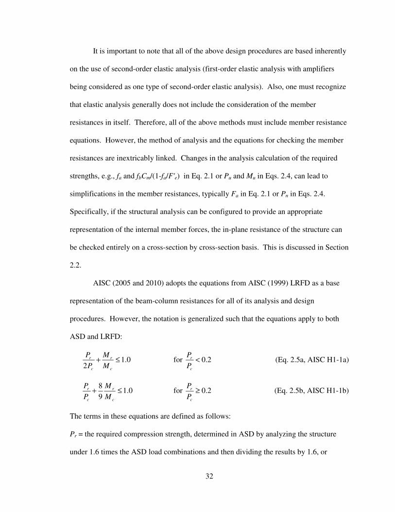
AISC (2005 and 2010) adopts the equations from AISC (1999) LRFD as a base

representation of the beam-column resistances for all of its analysis and design

procedures. However, the notation is generalized such that the equations apply to both

ASD and LRFD:

0.12

≤+

c

r

c

r

M

M

P

P for 2.0<

c

r

P

P (Eq. 2.5a, AISC H1-1a)

0.19

8≤+

c

r

c

r

M

M

P

P for 2.0≥

c

r

P

P (Eq. 2.5b, AISC H1-1b)

The terms in these equations are defined as follows:

Pr = the required compression strength, determined in ASD by analyzing the structure

under 1.6 times the ASD load combinations and then dividing the results by 1.6, or

33

determined in LRFD by analyzing the structure under the LRFD load combinations.

Mr = the required flexural strength, determined in ASD by analyzing the structure under

1.6 times the ASD load combinations and then dividing the results by 1.6, or determined

in LRFD by analyzing the structure under the LRFD load combinations.

Pc = the allowable or design compression resistance, given by Pn/Ωc in ASD or by φcPn in

LRFD, where Pn is the nominal compression resistance determined in accordance with

Chapter E.

Mc = the allowable or design flexural resistance, given by Mn/Ωb in ASD or by φbMn in

LRFD, where Mn is the nominal flexural resistance determined in accordance with

Chapter F.

φc and φb = resistance factors for axial compression and bending, both equal to 0.9.

Ωc and Ωb = factors of safety for axial compression and bending, both equal to 1.67.

For Equations 2.5a and b, another equation numbers are shown. In this dissertation,

AISC (2010) equation numbers are denoted by “AISC” followed by the equation number.

In many cases, Equations 2.5a and b provide a more liberal characterization of the beam-

column resistances than the multiple beam-column strength curves in AISC ASD (1989).

It should be noted that the 1.6 factor applied to determine the required

compression and flexural strengths under the ASD load combinations is smaller than the

column safety factor of 1.92 within the AISC ASD (1989) amplification of the flexural

stresses (see Eqs. 2.1 through 2.3). However, ASD-H1 also states that Cm shall be taken

as 0.85 in Eqs. 2.1 and 2.2 for frames subject to joint translation. This Cm value typically

underestimates the sidesway moment amplification effects (Salmon and Johnson 1996).

Nevertheless, the ASD moment amplifier summarized in Eq. 2.2 is still conservative in

34

many practical cases. This is because the predominant second-order effects are often

associated solely with the structure sidesway. Equation 2.1 applies a single amplifier

indiscriminately to the total flexural stresses from both non-sway and sidesway

displacements. The amplification factor procedure in AISC (1999) LRFD and AISC

(2005 and 2010) is more accurate, but involves a cumbersome subdivision of the analysis

into separate no-translation (nt) and lateral translation (lt) parts. Kuchenbecker et al.

(2004) and White et al. (2007a & b) outline an amplified first-order elastic analysis

approach that provides good accuracy for rectangular framing. This approach avoids the

above cumbersome attributes of the AISC (1999, 2005 & 2010) amplification factor

procedure

In the subsequent developments, it is useful to consider the characterization of

separate in-plane and out-of-plane beam-column resistances using Eqs. 2.5. The in-plane

beam-column resistance is addressed by neglecting out-of-plane flexural and/or flexural-

torsional buckling in the calculation of Pc and by neglecting lateral-torsional buckling in

the calculation of Mc. Correspondingly, the out-of-plane resistance is defined by

considering solely the out-of-plane flexural and flexural-torsional buckling limit states in

the determination of Pc (excluding the in-plane flexural buckling limit state), and by

considering all the potential flexural limit states (lateral-torsional buckling, flange local

buckling, tension flange yielding and general yielding) in the calculation of Mc. The

interaction of general yielding and/or local buckling with column flexural buckling is

included inherently within the calculation of both the in-plane and out-of-plane axial

strengths Pci and Pco. However, in the AISC (2005 and 2010) flexural resistance

equations, lateral-torsional buckling, compression flange local buckling and tension

35

flange yielding are handled as separate and independent limit states. The smaller

resistance from these separate limit states generally governs the flexural resistance. This

research recommends that the compression flange local buckling and tension flange

yielding limit states should be included in the calculation of the anchor point Mco for the

beam-column out-of-plane strength using Eqs. 2.5. Otherwise, potential influences of

compression flange local buckling or tension flange yielding on the out-of-plane beam-

column resistance are neglected.

2.2 Direct Analysis Method

Table 2.1 summarizes three specific overriding stability design procedures

defined in AISC (2010):

1. The direct analysis method, detailed in Sections C2 and C3,

2. The effective length method, detailed in Appendix 7, and

3. The first-order analysis method, detailed in Appendix 7.

Within the restrictions specified on their usage, and provided that effects such as

connection rotations or member axial and shear deformations are properly considered in

the analysis when these attributes are important, each of these methods is intended to

comprehensively address all of the effects listed in the beginning of Section 2.1.

As seen in Table 2.1, the direct analysis method is the only one of the above three

procedures that is generally applicable. In basic terms, this method involves the

following simple modifications to the second-order elastic analysis: (1) the use of a

reduced elastic stiffness and (2) for rectangular or tiered structures, the use of a notional

lateral load equal to a fraction of the vertical load at each level of the structure. These

two devices are adjustments to the second-order analysis that account for: (1) member

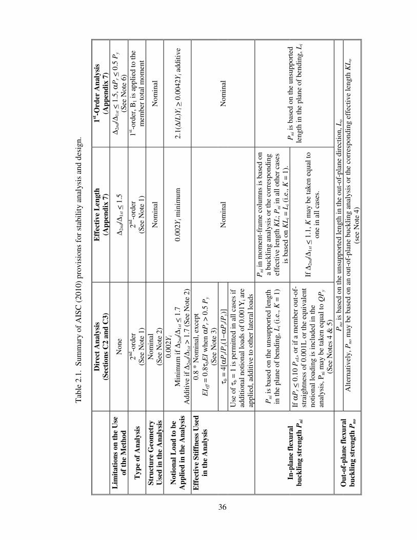
36

Tab

le 2

.1.

Sum

mar

y of

AIS

C (

2010

) pr

ovis

ions

for

sta

bilit

y an

alys

is a

nd d

esig

n.

D

irec

t A

naly

sis

(Sec

tion

s C

2 an

d C

3)

Eff

ecti

ve L

engt

h (A

ppen

dix

7)

1st-O

rder

Ana

lysi

s (A

ppen

dix

7)

Lim

itat

ions

on

the

Use

of

the

Met

hod

Non

e Δ

2nd/

Δ1s

t < 1

.5

Δ2n

d/Δ

1st <

1.5

, αP

r < 0

.5 P

y (S

ee N

ote

6)

Typ

e of

Ana

lysi

s

2nd-o

rder

(S

ee N

ote

1)

2nd-o

rder

(S

ee N

ote

1)

1st-o

rder

, B1

is a

pplie

d to

the

mem

ber

tota

l mom

ent

Stru

ctur

e G

eom

etry

U

sed

in th

e A

naly

sis

Nom

inal

(S

ee N

ote

2)

Nom

inal

N

omin

al

Not

iona

l Loa

d to

be

App

lied

in t

he A

naly

sis

0.00

2Yi

Min

imum

if Δ

2nd/

Δ1s

t < 1

.7

Add

itive

if Δ

2nd/

Δ1s

t > 1

.7 (

See

Not

e 2)

0.

002Y

i min

imum

2.

1(Δ

/L)Y

i > 0

.004

2Yi a

dditi

ve

Eff

ecti

ve S

tiff

ness

Use

d in

the

Ana

lysi

s 0.

8 *

Nom

inal

, exc

ept

EI e

ff =

0.8

τbE

I w

hen

αP

r > 0

.5 P

y (S

ee N

ote

3)

Nom

inal

N

omin

al

τb

= 4

[αP

r/Py(

1−α

Pr/P

y)]

Use

of

τb

= 1

is p

erm

itted

in a

ll ca

ses

if

addi

tion

al n

otio

nal l

oads

of

0.00

1Yi a

re

appl

ied,

add

itive

to o

ther

late

ral l

oads

In-p

lane

flex

ural

bu

cklin

g st

reng

th P

ni

Pni is

bas

ed o

n th

e un

supp

orte

d le

ngth

in

the

plan

e of

ben

ding

, Li (

i.e.,

K =

1)

Pni in

mom

ent-

fram

e co

lum

ns is

bas

ed o

n a

buck

ling

ana

lysi

s or

the

corr

espo

ndin

g ef

fect

ive

leng

th K

L; P

ni in

all

oth

er c

ases

is

bas

ed o

n K

Li =

Li (

i.e.,

K =

1).

P

ni is

bas

ed o

n th

e un

supp

orte

d le

ngth

in th

e pl

ane

of b

endi

ng, L

iIf

αP

r < 0

.10

PeL

, or

if a

mem

ber

out-

of-

stra

ight

ness

of

0.00

1L o

r th

e eq

uiva

lent

no

tiona

l loa

ding

is in

clud

ed in

the

anal

ysis

, Pni m

ay b

e ta

ken

equa

l to

QP

y (S

ee N

otes

4 &

5)

If Δ

2nd/

Δ1s

t < 1

.1, K

may

be

take

n eq

ual t

o on

e in

all

case

s.

Out

-of-

plan

e fl

exur

al

buck

ling

stre

ngth

Pno

Pno

is b

ased

on

the

unsu

ppor

ted

leng

th in

the

out-

of-p

lane

dir

ectio

n, L

o A

lter

nati

vely

, Pno

may

be

base

d on

an

out-

of-p

lane

buc

klin

g an

alys

is o

r th

e co

rres

pond

ing

effe

ctiv

e le

ngth

KL

o

(see

Not

e 4)

36

37

Not

es o

n T

able

2.1

:

Gen

eral

Not

e. Δ

2nd/

Δ1s

t is

the

ratio

of

the

2nd-o

rder

dri

ft to

the

1st-o

rder

dri

ft (

for

rect

angu

lar

fram

es, Δ

2nd/

Δ1s

t may

be

take

n as

B2

calc

ulat

ed b

y Se

ctio

n 8.

2.2)

. Δ

/L is

the

larg

est 1

st-o

rder

dri

ft f

rom

all

the

stor

ies

in th

e st

ruct

ure.

In

stru

ctur

es th

at h

ave

flex

ible

dia

phra

gms,

the

Δ/L

in e

ach

stor

y is

take

n as

the

aver

age

drif

t wei

ghte

d in

pro

port

ion

to th

e ve

rtic

al lo

ad, o

r al

tern

ativ

ely,

the

max

imum

dri

ft.

All

Δ2n

d/Δ

1st a

nd Δ

/L r

atio

s sh

all

be c

alcu

late

d us

ing

the

LR

FD lo

ad c

ombi

natio

ns o

r us

ing

a fa

ctor

of

α =

1.6

app

lied

to th

e gr

avity

load

s in

ASD

. T

he f

acto

r α

is 1

.0 f

or L

RFD

an

d 1.

6 fo

r A

SD.

The

term

Yi i

s th

e to

tal g

ravi

ty lo

ad a

pplie

d at

a g

iven

leve

l of

the

stru

ctur

e. P

eL is

the

mem

ber

elas

tic b

uckl

ing

resi

stan

ce b

ased

on

the

actu

al u

nsup

port

ed le

ngth

in th

e pl

ane

of b

endi

ng, π

2 EI/

L2 f

or p

rism

atic

mem

bers

.

Not

e 1.

Any

legi

tim

ate

met

hod

of s

econ

d-or

der

anal

ysis

that

incl

udes

bot

h P

Δ a

nd P

δ e

ffec

ts is

per

mit

ted,

incl

udin

g 1st

-ord

er a

naly

sis

with

am

plif

iers

. Se

ctio

n C

2.1

in A

ISC

(20

10)

addr

esse

s th

e co

nditi

ons

whe

n th

e P

δ e

ffec

ts c

an b

e ne

glec

ted.

In

the

Com

men

tary

of

Sect

ion

C2.

1,

mor

e de

tail

ed g

uide

line

s ar

e pr

ovid

ed th

e lim

its

whe

n a

PΔ

ana

lysi

s ca

n ad

equa

tely

cap

ture

the

Pδ e

ffec

ts u

sing

one

ele

men

t per

mem

ber

wit

h le

ss

than

5 a

nd 3

% e

rror

s in

the

side

sway

dis

plac

emen

ts a

nd th

e co

rres

pond

ing

inte

rnal

mom

ents

res

pect

ivel

y. T

he c

ases

add

ress

ed a

re s

way

col

umns

w

ith s

impl

y-su

ppor

ted

base

d co

nditi

ons,

sw

ay c

olum

ns w

ith

rota

tiona

l res

trai

nts

at b

oth

ends

, and

mem

bers

sub

ject

ed to

pre

dom

inan

tly

non-

sway

en

d co

nditi

ons.

If

the

spec

ifie

d lim

its

are

exce

eded

, eith

er m

ultip

le e

lem

ents

mus

t be

used

per

mem

ber

to o

btai

n ac

cura

te s

econ

d-or

der

inte

rnal

m

omen

ts in

gen

eral

fro

m a

P-l

arge

del

ta a

naly

sis,

or

a P

-sm

all d

elta

am

plif

ier

mus

t be

appl

ied

to th

e el

emen

t int

erna

l mom

ents

. K

aehl

er e

t al.

(201

0) p

rovi

de f

urth

er g

uide

lines

for

the

appr

opri

ate

num

ber

of P

Δ a

naly

sis

elem

ents

to a

dequ

atel

y ca

ptur

e th

e P

-δ e

ffec

ts. A

ccur

ate

gene

ral P

-Δ

anal

ysis

sol

utio

ns m

ay b

e ob

tain

ed b

y m

aint

aini

ng α

Pr <

0.0

2 P

e �, w

here

Pe �

is th

e el

astic

buc

klin

g lo

ad b

ased

on

the

idea

lized

sim

ply-

supp

orte

d en

d co

nditi

ons,

an

elem

ent l

engt

h �,

and

E if

the

anal

ysis

use

s th

e no

min

al s

tiffn

ess

and

0.8τ

bE if

the

dire

ct a

naly

sis

met

hod

is u

sed.

Not

e 2.

A n

omin

al in

itial

out

-of-

plum

bnes

s of

Δo/

L =

0.0

02 m

ay b

e us

ed d

irec

tly in

lieu

of

appl

ying

0.0

02Y

i min

imum

or

addi

tive

not

iona

l loa

ds.

Δ2n

d/Δ

1st s

peci

fied

in th

e di

rect

ana

lysi

s m

etho

d is

det

erm

ined

usi

ng th

e re

duce

d ef

fect

ive

stif

fnes

s sp

ecif

ied

in th

e fi

rst c

olum

n of

Tab

le 2

.1.

Not

e 3.

The

nom

inal

stif

fnes

s an

d ge

omet

ry s

houl

d be

em

ploy

ed f

or c

heck

ing

serv

icea

bilit

y li

mit

sta

tes.

The

red

uced

eff

ectiv

e st

iffn

ess

and

the

notio

nal l

oads

or

nom

inal

initi

al o

ut-o

f-pl

umbn

ess

are

requ

ired

onl

y in

con

side

ring

str

engt

h li

mit

sta

tes.

Not

e 4.

AIS

C (

2010

) do

es n

ot e

xplic

itly

stat

e th

is p

rovi

sion

in th

e co

ntex

t of

the

dire

ct a

naly

sis

met

hod.

Thi

s pr

ovis

ion

is e

ncom

pass

ed w

ithi

n th

e C

hapt

er C

req

uire

men

ts f

or g

ener

al s

tabi

lity

anal

ysis

and

des

ign,

whi

ch a

llow

any

met

hod

of a

naly

sis

and

desi

gn th

at a

ddre

sses

the

effe

cts

liste

d at

th

e be

ginn

ing

of S

ectio

n 2.

1.

Not

e 5.

The

larg

est u

ncon

serv

ativ

e er

ror

asso

ciat

ed w

ith th

e lim

it α

Pr <

0.1

0 P

eL is

app

roxi

mat

ely

five

per

cent

and

occ

urs

for

a si

mpl

y-su

ppor

ted,

co

ncen

tric

ally

load

ed c

olum

n w

ith

zero

mom

ent,

Q =

1, a

nd α

Pr =

0.1

0 P

eL =

φcP

y. T

he ta

rget

of

five

per

cent

max

imum

unc

onse

rvat

ive

erro

r is

ba

sed

on th

e or

igin

al d

evel

opm

ent o

f th

e A

ISC

LR

FD b

eam

-col

umn

stre

ngth

equ

atio

ns (

ASC

E 1

997;

Sur

ovek

-Mal

eck

and

Whi

te 2

004a

).

Not

e 6.

The

1st-o

rder

ana

lysi

s m

etho

d do

es n

ot a

ccou

nt f

or th

e in

flue

nce

of s

igni

fica

nt a

xial

com

pres

sion

in th

e ra

fter

s of

cle

ar-s

pan

fram

es.

The

refo

re, t

his

met

hod

stri

ctly

sho

uld

not b

e ap

plie

d fo

r th

e an

alys

is a

nd d

esig

n of

the

prim

ary

mom

ent f

ram

es in

thes

e ty

pes

of s

truc

ture

s.

37

38

inelasticity and reliability considerations at the strength limit of the most critical member

or members, as well as (2) the effects of a nominal initial out-of-plumbness Δo, within

fabrication and erection tolerances, on the internal forces and moments at the above

strength limit. The direct analysis method provides an improved representation of the

actual second-order inelastic forces and moments in the structure at the strength limit of

the most critical member or members. Due to this improvement in the calculation of the

internal forces and moments, AISC (2010) bases its calculation of Pni, the column

nominal strength for checking the in-plane resistance in Eqs. 2.5, on the actual

unsupported length in the plane of bending.

Interestingly, the use of the stub-column strength for Pni (QPy for columns with

slender compression elements) was actively considered in the development of the direct

analysis approach (Surovek-Maleck and White 2004a). Although this is a viable option,

it requires the modeling of out-of-straightness in the analysis for members subjected to

large axial compression (to properly capture in-plane limit states dominated by non-sway

column flexural-buckling). The modeling of member out-of-straightness adds an

additional level of complexity to the analysis, and in many steel structures, Pni based on

the actual unsupported length is only slightly smaller than QPy. Therefore, AISC (2010)

recommends the use of Pni based on the actual unsupported length. However, in many

metal building structural systems, the member axial loads are small enough such that the

beam-column resistance is represented accurately using Pni = QPy, without the inclusion

of any member out-of-straightness in the analysis. In other cases the modeling of

member out-of-straightness may be needed to accurately capture the strength limit.

39

2.3 Effective Length Method

The effective length method is in essence the traditional AISC method of design

since 1961, but with the addition of a notional minimum lateral load for gravity-load only

combinations. This minimum lateral load accounts for the influence of nominal

geometric imperfections on the brace forces, beam moments, connection moments and

in-plane member moments used for out-of-plane strength design of beam-columns. In

actuality, the effects of any physical out-of-plumbness exist for all load combinations.

However, these effects tend to be small and are overwhelmed by the effects of the

primary lateral loads in all the ASCE 7 lateral load combinations, as long as the

structure’s sidesway amplification is not excessive. Therefore, in the AISC (2005)

effective length method, the notional lateral loads are specified solely as minimum lateral

loads in the gravity load only combinations.

AISC (2010) disallows the use of the effective length method when the second-

order amplification of the sidesway displacements is larger than 1.7, i.e., Δ2nd /Δ1st > 1.7

(based on the nominal elastic stiffness of the structure). This is due to the fact that the

effective length method significantly underestimates the internal forces and moments in

certain cases when this limit is exceeded (Deierlein 2003 & 2004; Kuchenbecker et al.

2004; White et al. 2006). For structures with Δ2nd /Δ1st > 1.7, AISC (2010) requires the

use of the direct analysis method. Correspondingly, when using the direct analysis

approach with structures having Δ2nd /Δ1st < 1.7, AISC (2005) allows the Engineer to

apply the notional lateral loads (or the corresponding nominal out-of-plumbness) as

minimum values used solely with the gravity load only combinations.

40

For column and beam-column in-plane strength assessment in moment frames,

the effective length approach generally focuses on the calculation of the member axial

stresses Fei at incipient buckling of an appropriately selected model (the subscript “i” is

used to denote in-plane flexural buckling). This buckling model is usually some type of

subassembly that is isolated from the rest of the structural system (ASCE 1997).

Engineers often handle the elastic buckling stresses (Fei) implicitly, via the corresponding

column effective lengths KLi. The effective length is related to the underlying elastic

buckling stress via the relationship

2

2

)/( iiei rKL

EF

π= (Eq. 2.6a)

or

ei

iii F

rLEK

22 )//(π= (Eq. 2.6b)

In the effective length method, the influences of residual stresses, P-Δo effects and P-δo

effects are addressed implicitly in the calculation of Pni from the column strength

equations. These equations can be written either in terms of KLi or Fei (AISC 2010).

Unfortunately, the selection of an appropriate subassembly buckling model generally

requires considerable skill and engineering judgment. As a result, there is a plethora of

different buckling models and K factor calculations. In certain cases the different models

can produce radically different results. A few examples are provided below

In particular, one should note that a rigorous buckling analysis of the complete

structure does not in general provide an appropriate Fei or Ki. Members that have small

axial stress Fei at the buckling limit (relative to π2E/(Li/ri)2) tend to have high values for

41

Ki in Eq. 2.6b. In some cases, these large Ki values are justified while in other cases they

are not. If the member is indeed participating in the governing buckling mode, a large Ki

is justified. If the member is largely undergoing rigid-body motion in the governing

buckling mode, or if it has a relatively light axial load and is predominantly serving to

restrain the buckling of other members, a large Ki value is sometimes not justified. The

distinction between these two situations requires engineering judgment. Furthermore, the

concept of effective length is more obscure and less useful for general nonprismatic

members subjected to nonuniform axial compression.

Some of the situations requiring the greatest exercise of judgment to avoid

excessively large K values include: (1) columns in the upper stories of tall buildings, (2)

columns with highly flexible and/or weak connections and (3) beams or rafters in portal

frames, which may have significant axial compression due to the horizontal thrust at the

base of the frame. There is no simple way of quantifying the relative participation of a

given member in the overall buckling of the structure or subassembly under

consideration. Quantifying the participation requires an analysis of the sensitivity of the

buckling load to variations in the member sizes. Even if one conducted such an analysis,

there is no established metric for judging when Eq. 2.6b should or should not be used.

Engineers typically base their effective length calculations on story-by-story models to

avoid the first of the above situations. They idealize columns with weak and/or flexible

connections as pin-ended leaner columns with K = 1 to avoid the second situation.

Lastly, they often use K = 1, or K < 1 (counting on rotational restraint from the sidesway

columns), for design of the beams or rafters in portal frames, although the Fei of these

42

members obtained from an eigenvalue buckling analysis of the full structure may suggest

K > 1 via Eq. 2.6b.

The direct analysis method provides a simpler more accurate way of addressing

frame in-plane stability considerations. By including an appropriately reduced nominal

elastic stiffness, an appropriate nominal out-of-plumbness of the structure, and an

appropriate out-of-straightness (for members subjected to high axial loads) in the

analysis, the member length considerations can be completely removed from the

resistance side of the design equations. The member in-plane column strength term Pni is

simply taken equal to QPy. In-plane stability is addressed by estimating the required

internal cross-section strengths Pr and Mr directly from the analysis, and by comparing

these required strengths against appropriate cross-section resistances.

2.4 First-Order Analysis Method

The first-order analysis method, summarized in Table 2.1, is in essence a

simplified conservative application of the direct analysis approach, targeted at rectangular

or tiered building frames. This method involves:

• The implicit application of a conservative sidesway amplification factor of 1.5

(conservative as long as Δ2nd /Δ1st < 1.5) to the 1st-order story drift Δ/L or a nominal

initial out-of-plumbness of Δo/L = 0.002, whichever is larger. The 1st-order story drift

Δ/L is taken as the largest drift from all the stories in the structure, calculated under

the LRFD load combinations or with a factor of 1.6 applied to the gravity loads in

ASD. In structures that have flexible diaphragms, the Δ/L in each story is taken as the

average drift weighted in proportion to the vertical load, or alternatively, the

maximum drift

43

• The inclusion of the direct analysis stiffness reduction factor of 0.8 implicitly in the

second-order amplification of the above Δ/L or Δo/L, resulting in an amplification of

the sidesway displacements by a factor of 2.1 rather than 1.5.

• The assumption that all the stories of the structure have a sidesway deflection equal to

the above maximum amplified value.

• Inclusion of the corresponding P-Δ effects in the 1st-order analysis, by applying the P-

Δ shear forces corresponding to the above sidesway displacement at each level of the

structure (these P-Δ shears are applied in addition to any other lateral loads).

• Amplification of the corresponding total member moments obtained from the analysis

by the non-sway amplification factor B1 calculated as specified in Appendix 8 in

AISC (2010).

The first-order analysis method is restricted to frames with Δ2nd-order/Δ1st-order < 1.5 as well

as to cases where αPr < 0.5Py in all of the members whose flexural stiffnesses contribute

to the lateral stability of the structure. The limit αPr < 0.5Py prevents the application of

the method to structures where the sidesway stiffnesses are reduced significantly by

combined residual stress effects and large column axial compression.

Although the first-order analysis method can be useful for simplified analysis and

design of metal buildings in their longitudinal braced direction, this method does not

include the effects of rafter axial compression on the flexural response of the primary

moment frames. Also, this method is really just a direct analysis with a number of

simplifying assumptions. There are numerous other ways to apply direct analysis using

an approximate second-order analysis, many of which are less conservative than the

44

above approach. Therefore, the first-order analysis method is not considered further in

this research.

It should be noted that both the direct analysis method and effective length

method require a second-order elastic analysis. However, any legitimate method of

second-order elastic analysis is allowed, including first-order analysis with amplifiers,

when the amplifiers are sufficiently accurate. The stiffnesses and notional lateral loads

(or nominal geometric imperfections) used in the analysis are different in each of the

methods (see Table 2.1).

The beam-column out-of-plane resistance check is the same in both of the above

methods, albeit with different values of Pr and Mr. In AISC (2010), the simplest out-of-

plane beam-column resistance check is given by Eqs. 2.5 but with Pn = Pno, where Pno is

the out-of-plane flexural or flexural-torsional buckling strength of the member as a

concentrically-loaded column. Other enhanced beam-column out-of-plane strength

checks are provided in AISC (2010) and are discussed in Sections 2.6.2 and 3.4.1.

2.5 Fundamental Comparison of The Direct Analysis and Effective Length Methods

The differences between the direct analysis and the effective length methods are

predominantly in the way that they handle the beam-column in-plane strength check.

Figures 2.6a and 2.6b, adapted from Deierlein (2004), illustrate the fundamental

differences. Figure 2.6a shows a representative beam-column in-plane check using the

traditional effective length approach, i.e., the effective length method as outlined in Table

2.1 but with no limitations on the use of the method and with zero notional load. The

dashed curve in the figure is the AISC (2010) beam-column strength envelope, given by

Eqs. 2.5. The anchor point for this curve on the vertical axis, Pn(KLi), is the member

45

nominal axial strength determined using the effective length KLi (or equivalently, using

the member elastic buckling stress Fei as illustrated by Eqs. 2.6). The anchor point on the

horizontal axis is the member in-plane flexural resistance Mni, which is based in AISC

(2010) either on flange local buckling or general flexural yielding considerations. The

other two curves in the plot indicate the member internal axial force and moment under

increasing applied loads on the structure. The curve labeled “actual response” is

determined from an experiment or from a rigorous second-order distributed plasticity

analysis that accounts for all the significant stability effects, whereas the second curve is

from a second-order elastic analysis of the idealized straight and plumb, nominally elastic

structure. The actual response curve indicates larger moment than the second-order

elastic analysis curve due to the combined effects of partial yielding and geometric

imperfections, which are not included in the elastic second-order analysis. The maximum

value of P on the actual response curve (Pmax) is the largest value of the axial force that

the member can sustain at its stability limit. Correspondingly, the nominal design

strength is defined by the intersection of the force-point trace from the second-order

elastic analysis with the Pn(KLi) based envelope. The effective length provisions have

been calibrated such that this intersection point gives an accurate to conservative estimate

of the actual maximum strength.

The reduced stiffness and the notional load (or the corresponding nominal out-of-

plumbness) in the direct analysis method are calibrated to estimate the actual response

using a second-order elastic analysis. This is illustrated by Figure 2.6b, where the force-

point trace of the member internal axial force and moment from the second-order elastic

46

Figure 2.6. Comparison of beam-column strength interaction checks for (a) the effective length method (with zero notional load) and (b) the direct analysis method.

analysis (conducted using the reduced stiffness and notional lateral loads) is close to the

actual response plot. The calibration is done to achieve parity between the actual

compressive strength (indicated by Pmax on the actual response curve) and the nominal

design strength. By accounting for residual stress, partial member yielding and geometric

imperfection effects in the second-order elastic analysis, the resistance can be checked on

a member cross-section basis. That is, the anchor point on the vertical axis for the beam-

column strength envelope can be taken as QPy. As noted in Section 2.1, the use of Pni =

QPy requires that the member axial force must be smaller than 0.10PeL, or the use of a

member out-of-straightness of 0.001L in the analysis (to capture in-plane limit states

dominated by non-sway column flexural-buckling). AISC (2010) bases Pni on the actual

unsupported length in the plane of bending to avoid the need for consideration of member

out-of-straightness in a general frame analysis. The anchor point on the horizontal axis

(Mni) is the same in both the direct analysis and the effective length methods. In the

47

direct analysis method, the internal force and moment (P and M) and the strength

envelope (with the anchor points QPy and Mni) are an improved representation of the

actual response. Conversely, in the traditional effective length approach (i.e., the

effective length method with no notional load included), smaller idealized values of P

and M are checked against a correspondingly reduced beam-column strength interaction

curve. The direct analysis method accounts for the in-plane system stability effects

directly within the second-order analysis. Conversely, the effective length method

accounts for the in-plane system stability effects by reducing the member axial strength

Pni via an effective length KLi or the elastic buckling stress Fei obtained (implicitly or

explicitly) from an appropriately configured buckling analysis.

2.6 Illustrative Examples

The concepts discussed in Section 2.5 are best understood by considering a few

simple examples. The following subsections highlight two basic case studies, one taken

from the AISC (2005) TC10 and Specification Committee developments and the other

created by modifying an example design problem considered by the Specification

Committee. Other more detailed examples are presented by Maleck (2001), Maritinez-

Garcia (2002), Deierlein (2003), Surovek-Maleck and White (2004a & b), Kuchenbecker

et al. (2004), and White et al. (2006 and 2007a and b).

2.6.1 Cantilever Beam-Column

One of the simplest illustrations of the direct analysis and effective length

methods is the solution for the design strength of a fixed-base cantilever composed of a

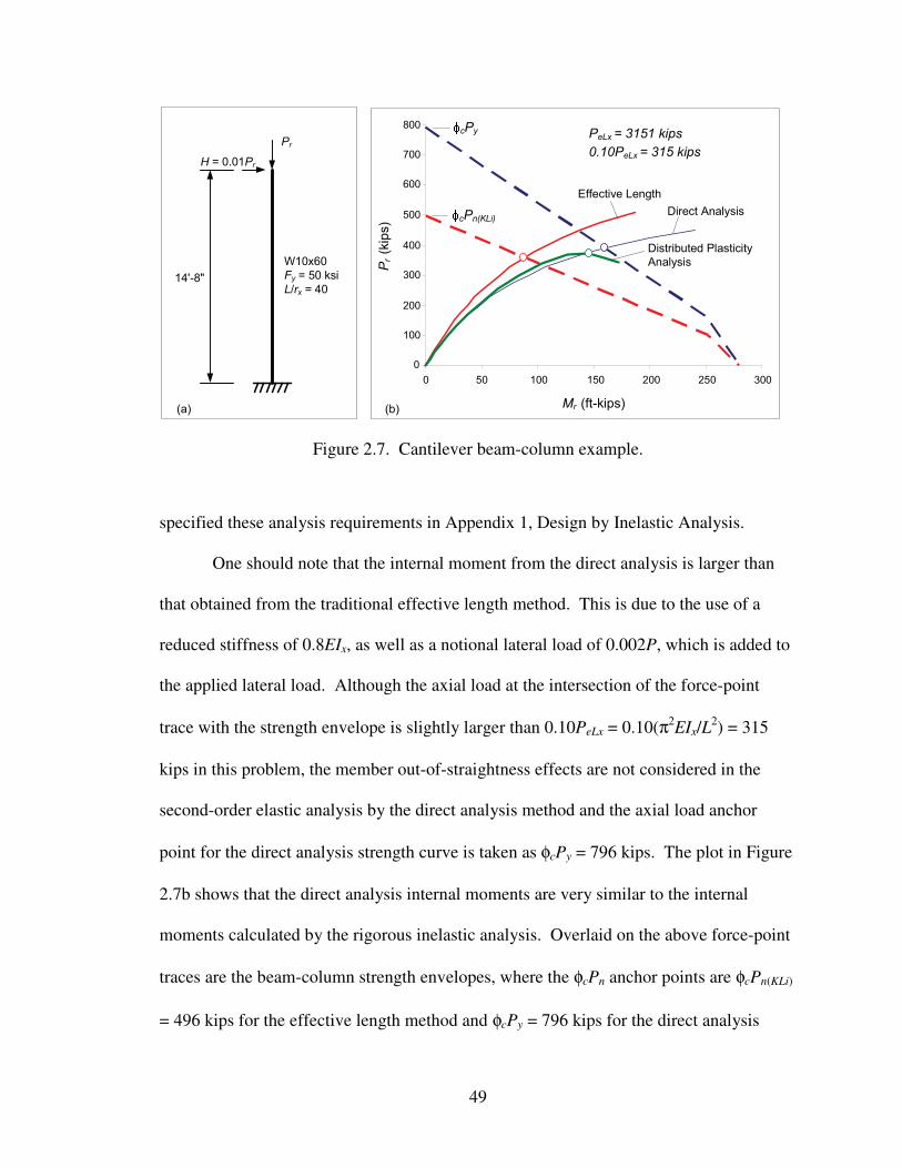
rolled wide-flange section. Figure 2.7a shows a W10x60 cantilever subjected to a

vertical load P and a proportional horizontal load of H = 0.01P, adapted from Deierlein

48

(2004). The bending is about the major axis and the member is braced out-of-plane such

that its in-plane resistance governs. In this problem, the member in-plane strength

governs in both the direct analysis and the effective length methods if the member is

braced at its top and bottom in the out-of-plane direction, the enhanced AISC (2005)

beam-column strength interaction equations are employed, and K = 0.7 is used for the

calculation of Pno, the column strength in the out-of-plane direction. The column

slenderness in the plane of bending is L/r = 40 based on the member’s actual length and

KL/r = 80 based on the effective length (with K = 2).

Figure 2.7b shows plots of the axial load versus the moment at the column base,

determined using three approaches: (1) the traditional effective length method (no

minimum notional lateral load included), (2) the direct analysis method, and (3) a

rigorous second-order distributed plasticity analysis. Load and Resistance Factor Design

(LRFD) is used with a resistance factor of φc = φb = 0.9 in each of these solutions. The

rigorous distributed plasticity analysis is based on a factored stiffness and strength of

0.9E and 0.9Fy, an out-of-plumbness and out-of-straightness on the geometry of 0.002L

and 0.001L respectively (oriented in the same direction as the bending due to the applied

loads), the Lehigh residual stress pattern (Galambos and Ketter 1959) with a maximum

compressive nominal residual stress at the flange tips of 0.3(0.9Fy) = 0.27Fy, and an

assumed elastic-perfectly plastic material stress-strain response. A small post-yield

stiffness of 0.001E is used for numerical stability purposes. These are established

parameters for calculation of benchmark design strengths in LRFD using a distributed

plasticity analysis (ASCE 1997; Martinez-Garcia 2002; Deierlein 2003; Maleck and

White 2003; Surovek-Maleck and White 2004b; White et al. 2006). AISC (2010)

49

�

���

���

���

���

���

���

��

��

� �� ��� ��� ��� ��� ���

��� ���� �� ������� �����������

�������� ����!���"�� ���

��#$%

��� ��&����

'�( ')(

������)*� +�,�����������������

��

���'��$!�-�(

����� ����������

����'!�-�(

��������� ���������

�������

Figure 2.7. Cantilever beam-column example.

specified these analysis requirements in Appendix 1, Design by Inelastic Analysis.

One should note that the internal moment from the direct analysis is larger than

that obtained from the traditional effective length method. This is due to the use of a

reduced stiffness of 0.8EIx, as well as a notional lateral load of 0.002P, which is added to

the applied lateral load. Although the axial load at the intersection of the force-point

trace with the strength envelope is slightly larger than 0.10PeLx = 0.10(π2EIx/L2) = 315

kips in this problem, the member out-of-straightness effects are not considered in the

second-order elastic analysis by the direct analysis method and the axial load anchor

point for the direct analysis strength curve is taken as φcPy = 796 kips. The plot in Figure

2.7b shows that the direct analysis internal moments are very similar to the internal

moments calculated by the rigorous inelastic analysis. Overlaid on the above force-point

traces are the beam-column strength envelopes, where the φcPn anchor points are φcPn(KLi)

= 496 kips for the effective length method and φcPy = 796 kips for the direct analysis

50

method.

The design strengths, determined as the combined P and M at the intersections

with the in-plane beam-column strength curves (Eqs. 2.5), are summarized in Table 2.2.

The ratios of the maximum base moments Mmax = HL + P(Δ + Δo) to the primary moment

HL indicate the magnitude of the second-order effects. The axial load at the direct

analysis strength limit, which is representative of the strength in terms of the total applied

load, is five percent higher than that obtained from the distributed plasticity analysis.

Conversely, the axial load at the effective length method beam-column strength limit is

four percent smaller than that obtained from the distributed plasticity solution. Both of

these estimates are within the targeted upper bound of five percent unconservative error

relative to the refined analysis established in the original development of the AISC LRFD

beam-column strength equations (ASCE 1997; Surovek-Maleck and White 2004a).

Table 2.2. Summary of calculated design strengths, cantilever beam-column example.

���� ���� ���� ��� ���� ����� ��� �������������� �

����� �������

������������ ��� ��� ���� ���� ����� ��!�"��������������� ��� �#� ���$

%��!���&����'����(��)��*�+���&��&��&�����&�!�

��*��,��+&!

��� $$ ���$ ����

The difference in the calculated internal moments is much larger. This difference

is expected since the effective length approach compensates for the underestimation of

the actual moments by reducing the value of the axial resistance term Pni, whereas the

direct analysis method imposes additional requirements on the analysis to obtain an

51

improved estimate of the actual internal moments. This more accurate calculation of the

internal moments also influences the design of the restraining members and their

connections. For instance, in this example, the column base moments from the direct

analysis method are more representative of the actual moments required at this position to

support the applied loads associated with the calculated member resistance. In this

regard, the direct analysis method provides a direct calculation of the required strengths

for all of the structural components. Conversely, the traditional effective length approach

generally necessitates supplementary requirements for calculation of the required

component strengths. AISC (2010) implements these supplementary requirements as (1)

a minimum notional lateral load to be applied with gravity-only load combinations and

(2) a limit on the use of the effective length method to frames having Δ2nd /Δ1st < 1.5, as

summarized in Table 2.1.

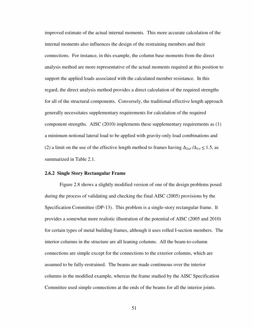
2.6.2 Single Story Rectangular Frame

Figure 2.8 shows a slightly modified version of one of the design problems posed

during the process of validating and checking the final AISC (2005) provisions by the

Specification Committee (DP-13). This problem is a single-story rectangular frame. It

provides a somewhat more realistic illustration of the potential of AISC (2005 and 2010)

for certain types of metal building frames, although it uses rolled I-section members. The

interior columns in the structure are all leaning columns. All the beam-to-column

connections are simple except for the connections to the exterior columns, which are

assumed to be fully-restrained. The beams are made continuous over the interior

columns in the modified example, whereas the frame studied by the AISC Specification

Committee used simple connections at the ends of the beams for all the interior joints.

52

This modification is performed to simulate typical conditions at the interior columns in

modular metal building frames. Due to the continuity of the beams, the exterior columns

are reduced from W12x72 sections in the AISC frame to W12x65 sections in the

modified example. Also, the beams are reduced from W24x68 sections in the exterior

spans and W27x84 sections in the interior spans of the AISC frame to W24x62 sections

in this example. The resulting modified frame has similar drift characteristics under

lateral loads; both the AISC example and the modified example satisfy a maximum drift

criterion of L/100 for the nominal (unfactored) wind load based on a first-order elastic

analysis. The strength behavior of the lateral load resisting beams and columns is similar

in both frames, with of course the exception of the beam continuity effects over the

interior columns in the modified design. The reader is referred to White et al. (2006) for a

detailed discussion of the behavior of the AISC frame.

Figure 2.8. Modified version of AISC single-story rectangular frame example DP-13.

53

The exterior columns in both examples are subjected to relatively light axial

loads, whereas they experience substantial gravity load moments as well as significant

wind load moments. Also, the frames have significant second-order effects, i.e.,

amplification of the member internal bending moments. The columns are braced in the

out-of-plane direction at their base and at the roof height. Simple base conditions are

assumed in both the in-plane and out-of-plane directions, and simple connections are

assumed in the out-of-plane direction at the column tops. The beams are assumed to be

braced sufficiently such that their flexural resistance is equal to Mp. This problem is

considered for the following LRFD load combinations:

1. Load Case 1 (LC1): 1.2 Dead + 1.6 Snow

2. Load Case 2 (LC2): 1.2 Dead + 0.5 Snow + 1.6 Wind

Figure 2.9 shows the applied fraction of the design loads versus the story drift for

these two load combinations on the modified single-story frame, obtained from a rigorous

second-order distributed plasticity analysis having the same attributes as described above

for the cantilever beam-column. The distributed plasticity analysis gives a maximum in-

plane capacity of 1.19 times the factored design load level for LC1 and 1.03 of the

factored design load level for LC2. Table 2.3 compares the fractions of the design loads

giving a unity check of 1.0 for the in-plane strength from Eqs. 2.5 for each of the design

methods to the above load capacities from the distributed plasticity analysis. In this

frame, the right-hand side exterior column is the most critical member in the effective

length check for both load cases and in the direct analysis check for LC2. In the direct

analysis check for LC1, the negative beam moment over the left-most interior column

gives the most critical strength check. One can observe that the direct analysis

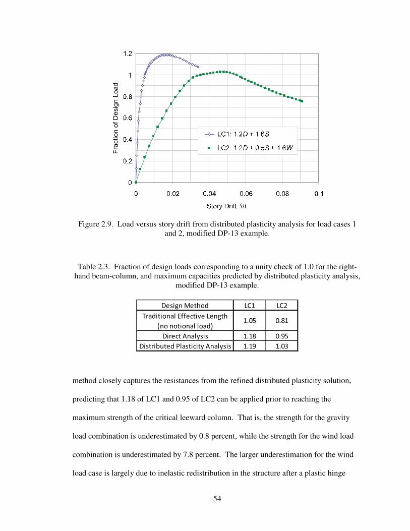
54

.�����/��/��� ������/�+

Figure 2.9. Load versus story drift from distributed plasticity analysis for load cases 1 and 2, modified DP-13 example.

Table 2.3. Fraction of design loads corresponding to a unity check of 1.0 for the right-hand beam-column, and maximum capacities predicted by distributed plasticity analysis,

modified DP-13 example.

��*��,��+&! )-� )-�

������������ ���$ ���� ����� ��!�"��������������� ���� ����

%��!���&����'����(��)��*�+���&��&��&�����&�!�

���� ��$�

method closely captures the resistances from the refined distributed plasticity solution,

predicting that 1.18 of LC1 and 0.95 of LC2 can be applied prior to reaching the

maximum strength of the critical leeward column. That is, the strength for the gravity

load combination is underestimated by 0.8 percent, while the strength for the wind load

combination is underestimated by 7.8 percent. The larger underestimation for the wind

load case is largely due to inelastic redistribution in the structure after a plastic hinge

55

forms at the top of the leeward column. However, there is little redundancy in the

structural system as the column strength limit is approached for the gravity load

combination. Nevertheless, the most critical member check for LC1 by direct analysis is

the beam negative moment check over the left-most interior column. The large elastic

negative bending moment at this location reaches the factored plastic moment resistance

of the beam φbMp at 1.10 of the design load. The distributed plasticity solution for LC1

indicates substantial inelastic redistribution from a beam plastic hinge at this location

prior to the structure reaching its strength limit at 1.19 of the design load. The right-most

exterior column is critical for all the other design checks by either the direct analysis or

the effective length methods.

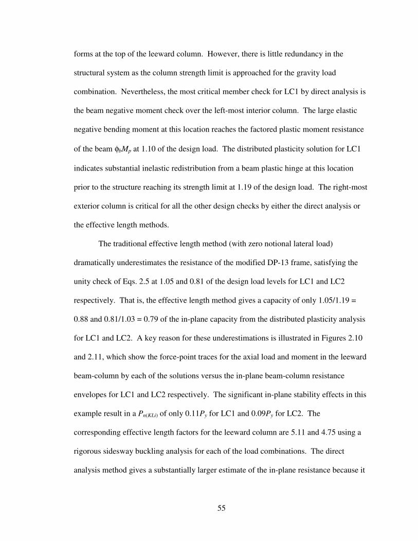
The traditional effective length method (with zero notional lateral load)

dramatically underestimates the resistance of the modified DP-13 frame, satisfying the

unity check of Eqs. 2.5 at 1.05 and 0.81 of the design load levels for LC1 and LC2

respectively. That is, the effective length method gives a capacity of only 1.05/1.19 =

0.88 and 0.81/1.03 = 0.79 of the in-plane capacity from the distributed plasticity analysis

for LC1 and LC2. A key reason for these underestimations is illustrated in Figures 2.10

and 2.11, which show the force-point traces for the axial load and moment in the leeward

beam-column by each of the solutions versus the in-plane beam-column resistance

envelopes for LC1 and LC2 respectively. The significant in-plane stability effects in this

example result in a Pn(KLi) of only 0.11Py for LC1 and 0.09Py for LC2. The

corresponding effective length factors for the leeward column are 5.11 and 4.75 using a

rigorous sidesway buckling analysis for each of the load combinations. The direct

analysis method gives a substantially larger estimate of the in-plane resistance because it

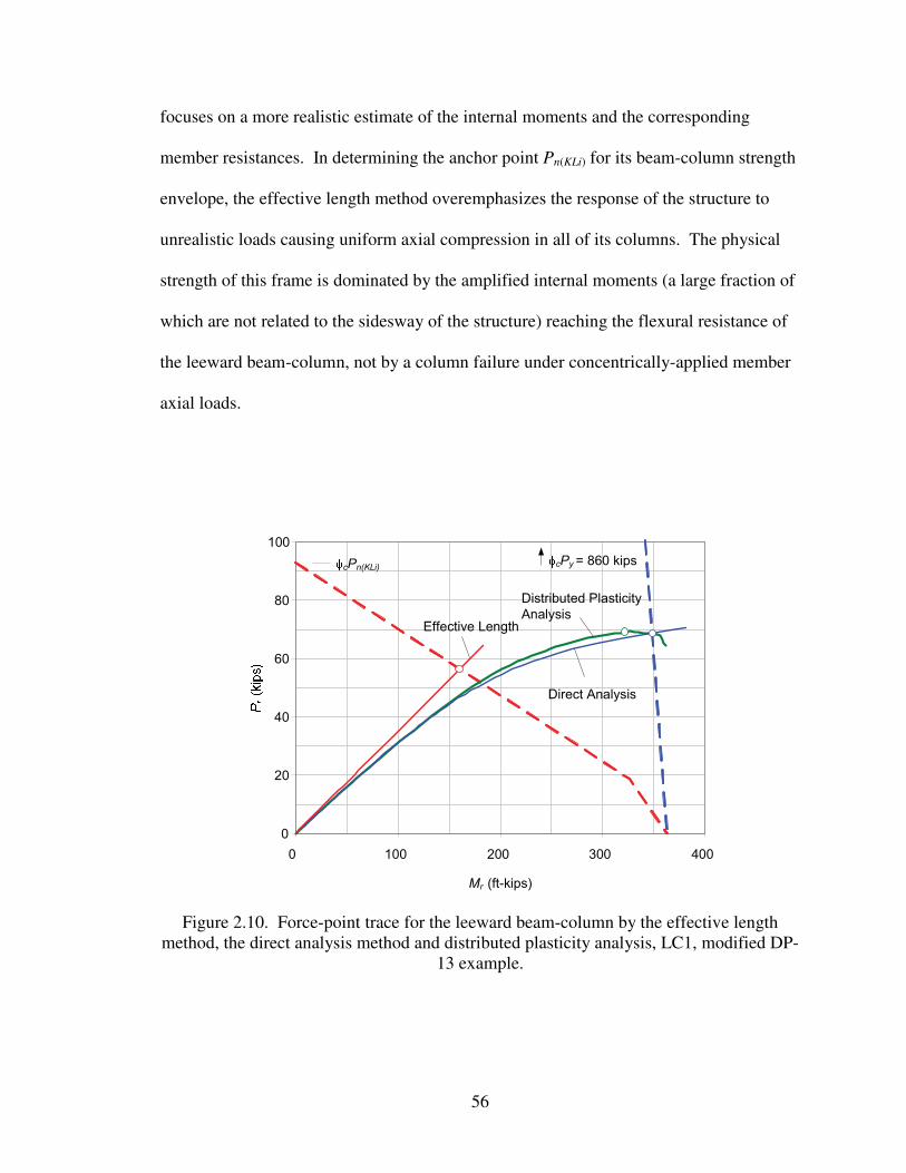
56

focuses on a more realistic estimate of the internal moments and the corresponding

member resistances. In determining the anchor point Pn(KLi) for its beam-column strength

envelope, the effective length method overemphasizes the response of the structure to

unrealistic loads causing uniform axial compression in all of its columns. The physical

strength of this frame is dominated by the amplified internal moments (a large fraction of

which are not related to the sidesway of the structure) reaching the flexural resistance of

the leeward beam-column, not by a column failure under concentrically-applied member

axial loads.

�

��

��

��

�

���

� ��� ��� ��� ���

��� ���� �� ����

��� �����������

������)*� +�,�����������������

��� ����!�-�

���'��$!�-�(

�������

Figure 2.10. Force-point trace for the leeward beam-column by the effective length method, the direct analysis method and distributed plasticity analysis, LC1, modified DP-

13 example.

57

�

��

��

��

�

���

� ��� ��� ��� ���

��� ���� �� ����

��� �����������

������)*� +�,�����������������

��� ����!�-�

���'��$!�-�(

����'!�-�(

�������

Figure 2.11. Force-point trace for the leeward beam-column by the effective length method, the direct analysis method and distributed plasticity analysis, LC2, modified DP-

13 example.

AISC (2010) provides the following enhanced beam-column strength interaction

equation for checking the out-of-plane resistance of doubly-symmetric rolled I-section

members subjected to single axis flexure and compression:

0.15.05.1

2

)1(

≤���

����

�+���

����

�−

=Cbcxb

r

co

r

co

r

MC

M

P

P

P

P (Eq. 2.7, AISC H1-2)

where Pco is the out-of-plane column strength, Mcx is the governing major-axis flexural

resistance of the member determined in accordance with Chapter F using Cb = 1, and Cb

is lateral-torsional buckling modification factor specified in Section F1. It should be

emphasized that the value of CbMcx(Cb=1) may be larger than φbMpx in LRFD or Mpx/Ωb in

ASD. Equation 2.7 is derived from the fundamental form for the out-of-plane lateral-

torsional buckling strength of doubly-symmetric I-section members in LRFD,

58

���

����

�φ

−���

����

�φ

−≤���

����

�

φ= ezc

r

noc

r

Cbnxbb

r

P

P

P

P

MC

M11

2

)1(

(Eq. 2.8, AISC C-H1-6)

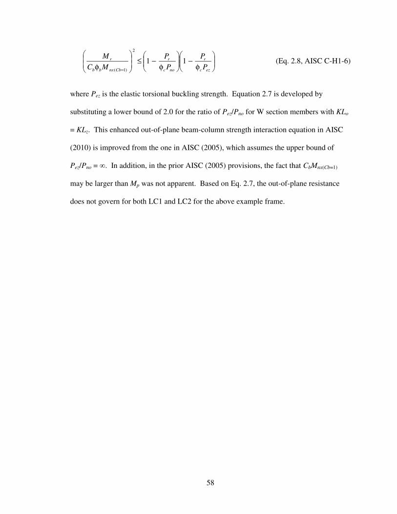
where Pez is the elastic torsional buckling strength. Equation 2.7 is developed by

substituting a lower bound of 2.0 for the ratio of Pez/Pno for W section members with KLo

= KLz. This enhanced out-of-plane beam-column strength interaction equation in AISC

(2010) is improved from the one in AISC (2005), which assumes the upper bound of

Pez/Pno = �. In addition, in the prior AISC (2005) provisions, the fact that CbMnx(Cb=1)

may be larger than Mp was not apparent. Based on Eq. 2.7, the out-of-plane resistance

does not govern for both LC1 and LC2 for the above example frame.