Stability via the Nyquist diagram

Range of gain for stability

Problem: For the unity feedback system be-

low, where

G(s) =K

s(s + 3)(s + 5),

find the range of gain, K, for stability, insta-

bility and the value of K for marginal stability.

For marginal stability, also find the frequency

of oscillation. Use the Nyquist criterion.

Figure above; Closed-loop unity feedback sys-

tem.

1

Solution:

G(jω) =K

s(s + 3)(s + 5)|s→jω

=−8Kω − j · K(15 − ω2)

64ω3 + ω(15 − ω2)2

When K = 1,

G(jω) =−8ω − j · (15 − ω2)

64ω3 + ω(15 − ω2)2

Important points:

Starting point: ω = 0, G(jω) = −0.0356 − j∞

Ending point: ω = ∞, G(jω) = 06 − 270◦

Real axis crossing: found by setting the imag-

inary part of G(jω) as zero,

ω =√

15, {− K

120, j0}

2

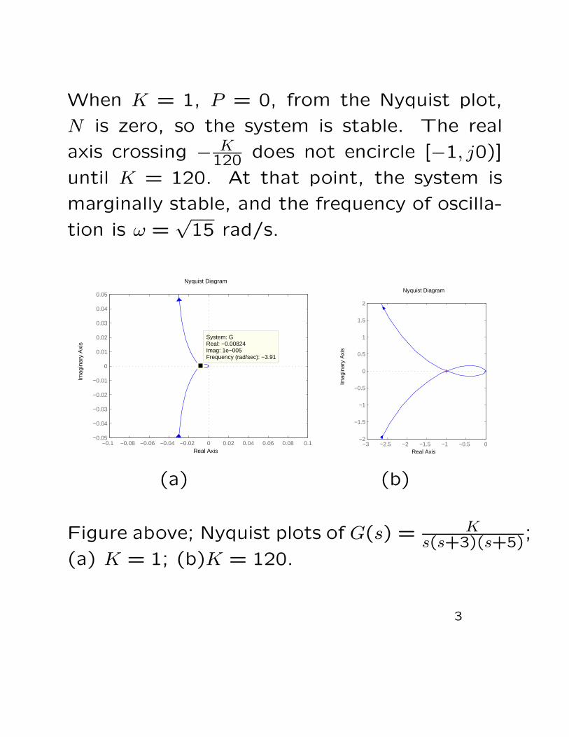
When K = 1, P = 0, from the Nyquist plot,

N is zero, so the system is stable. The real

axis crossing − K120 does not encircle [−1, j0)]

until K = 120. At that point, the system is

marginally stable, and the frequency of oscilla-

tion is ω =√

15 rad/s.

Nyquist Diagram

Real Axis

Imag

inar

y A

xis

−0.1 −0.08 −0.06 −0.04 −0.02 0 0.02 0.04 0.06 0.08 0.1−0.05

−0.04

−0.03

−0.02

−0.01

0

0.01

0.02

0.03

0.04

0.05

System: GReal: −0.00824Imag: 1e−005Frequency (rad/sec): −3.91

−3 −2.5 −2 −1.5 −1 −0.5 0−2

−1.5

−1

−0.5

0

0.5

1

1.5

2

Nyquist Diagram

Real Axis

Imag

inar

y A

xis

(a) (b)

Figure above; Nyquist plots of G(s) = Ks(s+3)(s+5)

;

(a) K = 1; (b)K = 120.

3

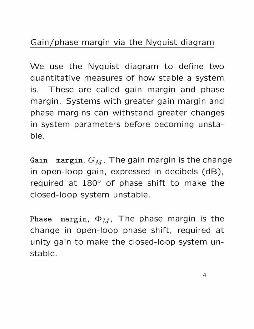
Gain/phase margin via the Nyquist diagram

We use the Nyquist diagram to define two

quantitative measures of how stable a system

is. These are called gain margin and phase

margin. Systems with greater gain margin and

phase margins can withstand greater changes

in system parameters before becoming unsta-

ble.

Gain margin, GM , The gain margin is the change

in open-loop gain, expressed in decibels (dB),

required at 180◦ of phase shift to make the

closed-loop system unstable.

Phase margin, ΦM , The phase margin is the

change in open-loop phase shift, required at

unity gain to make the closed-loop system un-

stable.

4

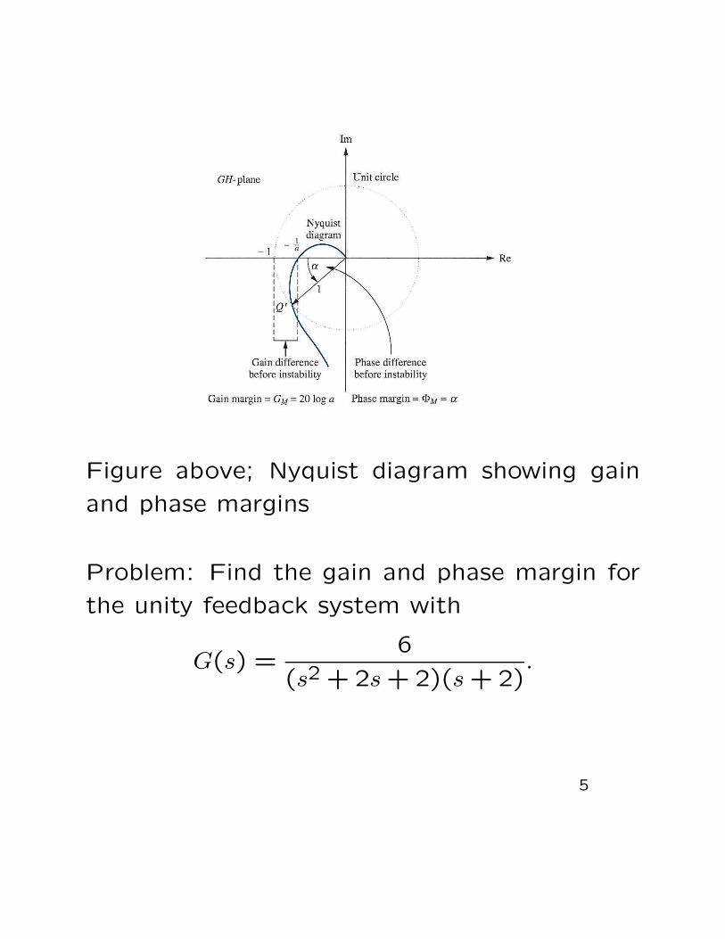
Figure above; Nyquist diagram showing gain

and phase margins

Problem: Find the gain and phase margin for

the unity feedback system with

G(s) =6

(s2 + 2s + 2)(s + 2).

5

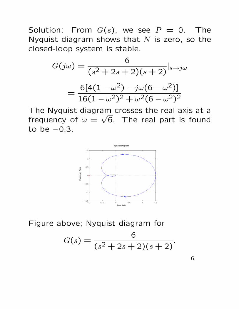
Solution: From G(s), we see P = 0. TheNyquist diagram shows that N is zero, so theclosed-loop system is stable.

G(jω) =6

(s2 + 2s + 2)(s + 2)|s→jω

=6[4(1 − ω2) − jω(6 − ω2)]

16(1 − ω2)2 + ω2(6 − ω2)2

The Nyquist diagram crosses the real axis at afrequency of ω =

√6. The real part is found

to be −0.3.

−1 −0.5 0 0.5 1 1.5−1.5

−1

−0.5

0

0.5

1

1.5

Nyquist Diagram

Real Axis

Imag

inar

y A

xis

Figure above; Nyquist diagram for

G(s) =6

(s2 + 2s + 2)(s + 2).

6

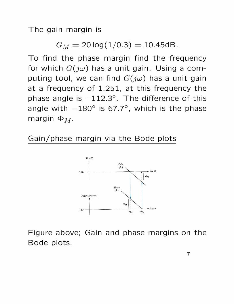
The gain margin is

GM = 20 log(1/0.3) = 10.45dB.

To find the phase margin find the frequency

for which G(jω) has a unit gain. Using a com-

puting tool, we can find G(jω) has a unit gain

at a frequency of 1.251, at this frequency the

phase angle is −112.3◦. The difference of this

angle with −180◦ is 67.7◦, which is the phase

margin ΦM .

Gain/phase margin via the Bode plots

Figure above; Gain and phase margins on the

Bode plots.

7

Problem: Let a unit feedback system have

G(s) =K

(s + 2)(s + 4)(s + 5).

Use Bode plots to determine the range of gain

within which the system is stable. If K = 200

find the gain margin and the phase margin.

The low frequency gain is found by setting s to

zero. Thus the Bode magnitude plots starts

at K/40. For convenience set K = 40, so

that the log-magnitude plots starts at 0dB. At

each break frequency, 2, 4 and 5, a slope of

-20dB/decade is added.

The phase diagram starts at 0◦ until 0.2rad/s

(a decade below the break frequency of 2),

the curve decreases at a slope of 45◦/decadeat each subsequent frequency at 0.4rad/s and

0.5rad/s (a decade below the break frequency

of 4 and 5 respectively). Finally at 20rad/s,

40rad/s and 50rad/s (a decade above the break

frequencies of 2,4,5), a slope of +20dB/decade

is added, until the curve levels out.

8

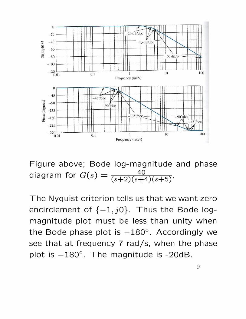
Figure above; Bode log-magnitude and phase

diagram for G(s) = 40(s+2)(s+4)(s+5)

.

The Nyquist criterion tells us that we want zero

encirclement of {−1, j0}. Thus the Bode log-

magnitude plot must be less than unity when

the Bode phase plot is −180◦. Accordingly we

see that at frequency 7 rad/s, when the phase

plot is −180◦. The magnitude is -20dB.

9

Thus an increase of 20dB is possible before the

system becomes unstable, which is a gain of

10, so the gain for instability is K > 10× 40 =

400.

If K = 200 (five times greater than K = 40),

the magnitude plot would be 20 log5 = 13.98dB

higher, as the Bodes plots was scaled to a gain

of 40.

At −180◦, the gain is −20+13.98 = −6.02dB,

so GM = 6.02dB.

To find phase margin, we look on the mag-

nitude plot for the frequency where the gain

is 0dB. As the plot should be 13.98dB higher,

so we look at −13.98dB crossing to find the

frequency is 5.5rad/s. At this frequency, the

phase angle is −165◦. Thus

ΦM = −165◦ − (−180)◦ = 15◦.

10