Stabilization—An Alternative to Double-Negation Translation for

Classical Natural Deduction

Ralph Matthes

matthes@informatik.uni-muenchen.de

Lehr- und Forschungseinheit fur theoretische Informatik

Institut fur Informatik der Universitat Munchen

Oettingenstraße 67, D-80538 Munchen

January 19, 2004

Abstract

A new proof of strong normalization of Parigot’s second-order λµ-calculus is given by areduction-preserving embedding into system F (second-order polymorphic λ-calculus). The mainidea is to use the least stable supertype for any type. These non-strictly positive inductive typesand their associated iteration principle are available in system F, and allow to give a translationvaguely related to CPS translations (corresponding to Kolmogorov’s double-negation embeddingof classical logic into intuitionistic logic). However, they simulate Parigot’s µ-reductions whereasCPS translations hide them.

As a major advantage, this embedding does not use the idea of reducing stability (¬¬A → A)to that for atomic formulae. Therefore, it even extends to positive fixed-point types.

The article expands on “Parigot’s Second-Order λµ-Calculus and Inductive Types” (Confer-ence Proceedings TLCA 2001, Springer LNCS 2044) by the author.

1 Introduction

If ¬¬A → A is provable, then A is called stable. Stability of all A is the key characteristic ofclassical logic. In the framework of intuitionistic logic, classical features can be added in severalways. We concentrate on “reductio ad absurdum” (RAA), i. e., proof by contradiction: If falsityis provable from the negation of A, then A is provable.

Natural deduction systems can be formulated—via the Curry-Howard-isomorphism—as lamb-da calculi. Here, we are interested in second-order logic, hence in second-order (polymorphic)lambda-calculus, also called system F.

System F is a term rewrite system, consequently also its extension by RAA comes withrewrite rules: we may speak about operationalized classical logic. The most well known suchsystem is Parigot’s λµ-calculus, and it is strongly normalizing [Par93, Par97], i. e., admits noinfinite reduction sequences starting with a typable term. Its µ-reduction rules describe howRAA for composite types can be reduced to RAA for the constituent types. In the case ofimplication, this corresponds to the fact that stability of A → B follows intuitionistically fromstability of B.

In [Mat01], an extension of system F by a least stable supertype ]A—called the stabilizationof A—for any type A, has been studied for the purpose of reproving strong normalization ofParigot’s second-order λµ-calculus.

In the present article, this approach is refined to also cover λµ-calculus in the formulationof de Groote [dG94]. Also typing issues are considered, in the sense that typing a la Church is

1

used instead of fully type-decorated terms. An important part of this article is the comparisonwith other approaches to prove strong normalization of second-order classical natural deductionfrom that of system F. For direct proofs of strong normalization through logical predicates—even capturing sums/disjunction with permutative/commuting conversions—see the account in[Mat04].

In a nutshell, [Mat01] has been extended

• to Church typing instead of full type annotations (with subtle problems leading to thenotion of “refined embedding”—Definition 2—and associated substitution rules),

• to λµ-calculus in de Groote’s formulation (with ⊥ being a regular type),

• by a comparison of stabilization with double negation,

• by a motivation of µ-reduction rules and a presentation of the method by Joly [Jol97],

• by an explanation why translations fail with Curry-style typing or just with plain classicalnatural deduction (without Parigot’s “special substitution”),

• by a discussion of the recent criticism of CPS-translations by Nakazawa and Tatsuta[NT03].

The article is structured as follows: In section 2, system F and second-order classical naturaldeduction are defined. Section 3 contains the definition of the system of I] with the leaststable supertype ]A for every type A and its impredicative encoding in F. It also containsa comparison of ]A and ¬¬A. Section 4 is the central part: It is first shown that the morenaive system F¬ of classical natural deduction cannot be embedded into F, then λµ-calculusis defined and successfully embedded in I]. Plenty of discussion material is given in section 5:After a presentation of Joly’s embedding, which is based on the idea of reducing stability tothat for atomic formulae (= type variables), an extension to fixed-points is given where Joly’smethod cannot be seen to work—unlike our stabilization. Even least fixed-points are treated.Finally, the article by Nakazawa and Tatsuta is discussed under the heading “Embeddings inContinuation-Passing Style?”.

Acknowledgments to Andreas Abel and Klaus Aehlig for fruitful discussions on the sub-ject.

2 Second-Order Natural Deduction

In this article, natural deduction is always represented by the help of lambda terms. For second-order natural deduction, the basic—intuitionistic—system is F [Gir72], which is defined in thefirst part of this section. Mostly, notation is given that is used throughout the article.

In the second part, F is extended by “reductio ad absurdum” (RAA), which is again just afixing of notation. In addition, an argument is given why F itself fails to be “classical”, and thereduction rules for RAA—which are a variation on those of λµ-calculus [Par92]—are motivatedby the reduction of stability for composite formulas/types to that for atoms/type variables.

2.1 System F

System F is the polymorphic lambda-calculus whose normalization has first been shown byGirard [Gir72]. In a proof-theoretic reading, F provides proof terms for intuitionistic second-order propositional logic in natural deduction style, and also considers proof transformationrules. Normalization for second-order systems does not yield the subformula property butnevertheless guarantees logical consistency and allows, e. g., to conclude that F is not classical—see below. In the programming language perspective, normalization is the calculation of valuesfor terms inhabiting a concrete datatype. And F is a (functional) programming language inwhich datatypes can be represented [BB85].

We define system F and recall some of its basic metatheoretic properties.

2

Types. (Denoted by uppercase letters.) Metavariable X ranges over an infinite set TV oftype variables.

A, B, C, D ::= X | ⊥ | A → B | ∀X.A

The occurrences of X in A are bound in ∀X.A. We identify types whose de Bruijn representationscoincide. Let FV(A) be the set of free type variables in A. The type ⊥ just serves as a constantin F. It is used to define ¬A := A → ⊥. Note that intuitionistic falsum is already present inthe pure system: ∀X.X has “ex falsum quodlibet” by trivial universal elimination.

Terms. (Denoted by lowercase letters.) The metavariable x ranges over an infinite set ofterm variables.

r, s, t ::= x | λxA.t | r s | ΛX.t | r B

The occurrences of x in t are bound in λxA.t. Also, the occurrences of type variable X in tare bound in ΛX.t We identify α-equivalent terms, that is, terms whose bound type and termvariables are consistently renamed. Capture-avoiding substitution of a term s for a variablex in term r is denoted by r[x := s]. Analogously, we define type substitution A[X := B]and substitution t[X := B] of type B for type variable X in term t. We think of terms asparse trees according to the above grammar rules and insert parentheses in case of ambiguities,especially around the application r s. But we will omit them as much as possible and assumethat application associates to the left. Hence, we write rs1 . . . sn for the parenthesized term(. . . (rs1) . . . sn)—also for types instead of terms si. We abbreviate idA := λxA.x, the identityon A.

Contexts. They are finite sets of pairs (x : A) of term variables and types and will be denotedby Γ. Term variables in a context Γ are assumed to be distinct, and the notation Γ, x : A shallindicate Γ ∪ {(x : A)} where x does not occur in Γ. Write FV(Γ) :=

⋃

(x:A)∈Γ FV(A).

Well-typed terms. Γ ` t : A is inductively defined by

(x :A) ∈ Γ

Γ ` x : A

Γ, x :A ` t : B

Γ ` λxA.t : A → B

Γ ` r : A → B Γ ` s : A

Γ ` r s : B

as for simply-typed lambda-calculus, and by the two rules for the universal quantifier whose useis traced in the terms (unlike formulations in a style a la Curry):

Γ ` t : A

Γ ` ΛX.t : ∀X.Aif X /∈ FV(Γ)

Γ ` r : ∀X.A

Γ ` r B : A[X := B]

A term t is typable if there are Γ and A such that Γ ` t : A. Write ` t : A for ∅ ` t : A. Ifthere is a term t with ` t : A, the type A is inhabited. Evidently, if Γ ` t : A and Γ ⊆ Γ′ for thecontext Γ′, then Γ′ ` t : A as well, i. e., weakening is an admissible typing rule. In the sequel,this word will be reserved for the rule

Γ ` t : Bx not declared in Γ

Γ, x : A ` t : B

It is also easy to see that the following cut rules are admissible typing rules:

Γ, x : A ` t : B Γ ` s : A

Γ ` t[x := s] : B

Γ ` t : B

Γ[X := A] ` t[X := A] : B[X := A]

Here, Γ[X := A] := x1 : B1[X := A], . . . , xn : Bn[X := A] for Γ = x1 : B1, . . . , xn : Bn.

3

Reduction. The one-step reduction relation t −→ t′ between terms t and t′ is defined as theclosure of the following axioms under all term constructors.

(λxA.t) s −→β t[x := s](ΛX.t) B −→β t[X := B]

We denote the transitive closure of −→ by −→+ and the reflexive-transitive closure by −→∗. Itis clear that r −→ r′ implies r[x := s] −→ r′[x := s] and s[x := r] −→∗ s[x := r′].

Normal terms. Inductively define the set NF of normal forms by:

• If, for all i ∈ {1, . . . , n}, either si ∈ NF or si is a type, then xs1 . . . sn ∈ NF.

• If t ∈ NF then λxA.t ∈ NF and ΛX.t ∈ NF.

It is easy to see that the terms in NF are exactly those terms t such that no t′ exists witht −→ t′, i. e., the normal forms are the normal terms.

Metatheoretic properties.

Lemma 1 (Subject Reduction) If Γ ` t : A and t −→ t′ then Γ ` t′ : A.

Proof This only requires the cut rules above. Subject reduction would be much more difficultin a formulation with typing a la Curry. �

Lemma 2 (Local Confluence) F is locally confluent, i. e., if r −→ r1, r2 then there is a termt such that r1, r2 −→∗ t.

Proof There are no critical pairs. �

It is well known that F is even confluent, i. e., −→∗ is locally confluent.

Lemma 3 (Strong Normalization) If Γ ` t : A then there is no infinite reduction sequencet −→ t1 −→ t2 −→ . . . In other words, every typable term is strongly normalizing.

This deep result is known since Tait’s adaptation [Tai75] of Girard’s proof of weak normalization[Gir72].

2.2 Classical Natural Deduction

It is well known that system F is not classical: There is no closed term of type ¬¬X → X ,for X any type variable. (This is equivalent to the non-existence of a closed term of type∀X.¬¬X → X .)

A proof can be obtained as follows. If, to the contrary, there were such a term rc, one wouldalso get a closed term rp of type (¬X → X) → X , which amounts to the Peirce law: Set

rp := λx¬X→X . rc (λy¬X .y (x y)).

By normalization of F, there would also be a closed normal term r of type (¬X → X) → X .Several steps of reasoning about normal terms would yield that r = λx¬X→X . x (λzX .s) withs a normal term, and x : ¬X → X, z : X ` s : ⊥. This is plainly impossible, by inspection ofnormal forms.1

Therefore, F has to be extended in order to be classical. Following Prawitz [Pra65, Pra71],system F¬ will now be based on “reductio ad absurdum” (RAA): If one can derive absurdityfrom the assumption ¬A, then A obtains. A term notation for a first-order system in thisspirit has been proposed by Rehof and Sørensen [RS94], and later on even for pure type systems

1This proof—with the detour through Peirce’s law—also works in case that ⊥ is set to ∀Y.Y , i. e., for the systemwith built-in ex falsum quodlibet ∀X.⊥ → X.

4

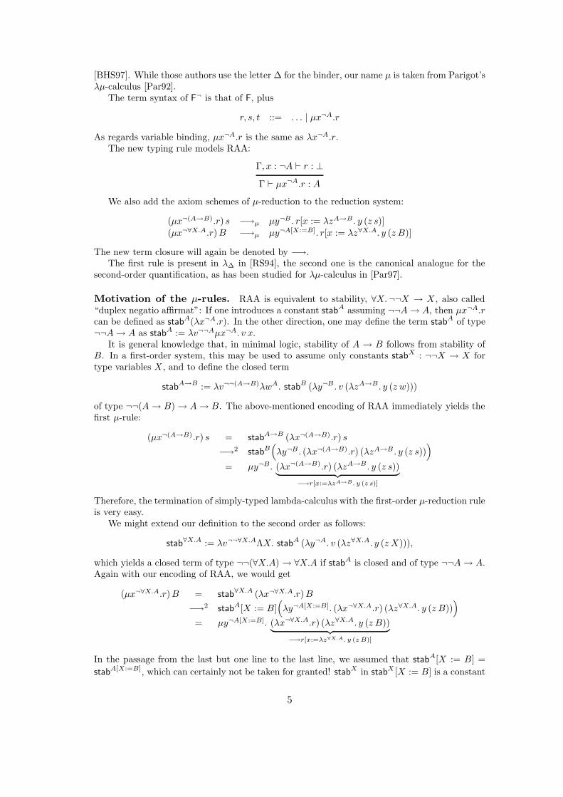
[BHS97]. While those authors use the letter ∆ for the binder, our name µ is taken from Parigot’sλµ-calculus [Par92].

The term syntax of F¬ is that of F, plus

r, s, t ::= . . . | µx¬A.r

As regards variable binding, µx¬A.r is the same as λx¬A.r.The new typing rule models RAA:

Γ, x : ¬A ` r : ⊥

Γ ` µx¬A.r : A

We also add the axiom schemes of µ-reduction to the reduction system:

(µx¬(A→B).r) s −→µ µy¬B . r[x := λzA→B . y (z s)]

(µx¬∀X.A.r) B −→µ µy¬A[X:=B]. r[x := λz∀X.A. y (z B)]

The new term closure will again be denoted by −→.The first rule is present in λ∆ in [RS94], the second one is the canonical analogue for the

second-order quantification, as has been studied for λµ-calculus in [Par97].

Motivation of the µ-rules. RAA is equivalent to stability, ∀X.¬¬X → X , also called“duplex negatio affirmat”: If one introduces a constant stabA assuming ¬¬A → A, then µx¬A.rcan be defined as stabA(λx¬A.r). In the other direction, one may define the term stabA of type¬¬A → A as stabA := λv¬¬Aµx¬A. v x.

It is general knowledge that, in minimal logic, stability of A → B follows from stability ofB. In a first-order system, this may be used to assume only constants stabX : ¬¬X → X fortype variables X , and to define the closed term

stabA→B := λv¬¬(A→B)λwA. stab

B (λy¬B . v (λzA→B . y (z w)))

of type ¬¬(A → B) → A → B. The above-mentioned encoding of RAA immediately yields thefirst µ-rule:

(µx¬(A→B).r) s = stabA→B (λx¬(A→B).r) s

−→2 stabB(

λy¬B . (λx¬(A→B).r) (λzA→B . y (z s)))

= µy¬B. (λx¬(A→B).r) (λzA→B . y (z s))︸ ︷︷ ︸

−→r[x:=λzA→B. y (z s)]

Therefore, the termination of simply-typed lambda-calculus with the first-order µ-reduction ruleis very easy.

We might extend our definition to the second order as follows:

stab∀X.A := λv¬¬∀X.AΛX. stabA (λy¬A. v (λz∀X.A. y (z X))),

which yields a closed term of type ¬¬(∀X.A) → ∀X.A if stabA is closed and of type ¬¬A → A.Again with our encoding of RAA, we would get

(µx¬∀X.A.r) B = stab∀X.A (λx¬∀X.A.r) B

−→2 stabA[X := B](

λy¬A[X:=B]. (λx¬∀X.A.r) (λz∀X.A. y (z B)))

= µy¬A[X:=B]. (λx¬∀X.A.r) (λz∀X.A. y (z B))︸ ︷︷ ︸

−→r[x:=λz∀X.A. y (z B)]

In the passage from the last but one line to the last line, we assumed that stabA[X := B] =

stabA[X:=B], which can certainly not be taken for granted! stabX in stabX [X := B] is a constant

5

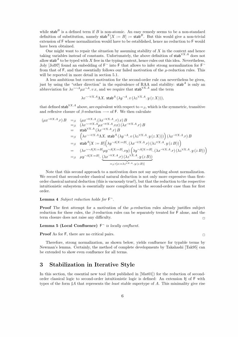
while stabB is a defined term if B is non-atomic. An easy remedy seems to be a non-standarddefinition of substitution, namely stabX [X := B] := stabB . But this would give a non-trivialextension of F whose normalization would have to be established, hence no reduction to F wouldhave been obtained.

One might want to repair the situation by assuming stability of X in the context and hencetaking variables instead of constants. Unfortunately, the above definition of stab∀X.A does notallow stabA to be typed with X free in the typing context, hence rules out this idea. Nevertheless,Joly [Jol97] found an embedding of F¬ into F that allows to infer strong normalization for F¬

from that of F, and that essentially follows our failed motivation of the µ-reduction rules. Thiswill be reported in more detail in section 5.1.

A less ambitious but correct motivation for the second-order rule can nevertheless be given,just by using the “other direction” in the equivalence of RAA and stability: stabA is only anabbreviation for λv¬¬Aµx¬A. v x, and we require that stab∀X.A and the term

λv¬¬∀X.AΛX. stabA (λy¬A. v (λz∀X.A. y (z X))),

that defined stab∀X.A above, are equivalent with respect to =β , which is the symmetric, transitiveand reflexive closure of β-reduction −→ of F. We then calculate

(µx¬∀X.A.r) B =β (µx¬∀X.A.(λx¬∀X.A. r) x) B=β (λv¬¬∀X.Aµx¬∀X.A.vx) (λx¬∀X.A.r) B

= stab∀X.A (λx¬∀X.A.r) B

=β

(

λv¬¬∀X.AΛX. stabA (λy¬A. v (λz∀X.A. y (z X))))

(λx¬∀X.A.r) B

=β stabA[X := B](

λy¬A[X:=B]. (λx¬∀X.A.r) (λz∀X.A. y (z B)))

= (λv¬¬A[X:=B]µy¬A[X:=B].vy)(

λy¬A[X:=B]. (λx¬∀X.A.r) (λz∀X.A. y (z B)))

=β µy¬A[X:=B]. (λx¬∀X.A.r) (λz∀X.A. y (z B))︸ ︷︷ ︸

=β r[x:=λz∀X.A. y (z B)]

Note that this second approach to a motivation does not say anything about normalization.We record that second-order classical natural deduction is not only more expressive than first-order classical natural deduction (this is vacuously true!), but that the reduction to the respectiveintuitionistic subsystem is essentially more complicated in the second-order case than for firstorder.

Lemma 4 Subject reduction holds for F¬.

Proof The first attempt for a motivation of the µ-reduction rules already justifies subjectreduction for these rules, the β-reduction rules can be separately treated for F alone, and theterm closure does not raise any difficulty. �

Lemma 5 (Local Confluence) F¬ is locally confluent.

Proof As for F, there are no critical pairs. �

Therefore, strong normalization, as shown below, yields confluence for typable terms byNewman’s lemma. Certainly, the method of complete developments by Takahashi [Tak95] canbe extended to show even confluence for all terms.

3 Stabilization in Iterative Style

In this section, the essential new tool (first published in [Mat01]) for the reduction of second-order classical logic to second-order intuitionistic logic is defined: An extension I] of F withtypes of the form ]A that represents the least stable supertype of A. This minimality give rise

6

to an iteration principle that explains the heading “stabilization in iterative style”. Althoughthis is the only way stabilization is treated in the present article, this name is chosen in order todistinguish it from another approach to stabilization capable of capturing sums with permutativeconversions, to be reported elsewhere.

The first part is devoted to the definition of I], and to its (impredicative) justification interms of F, whose strong normalization is inherited through an embedding. In the second part,we find a retract embedding of ¬¬A into ]A, giving a link to the Kolmogorov translation onwhich CPS-translations are based.

3.1 Definition of System I]

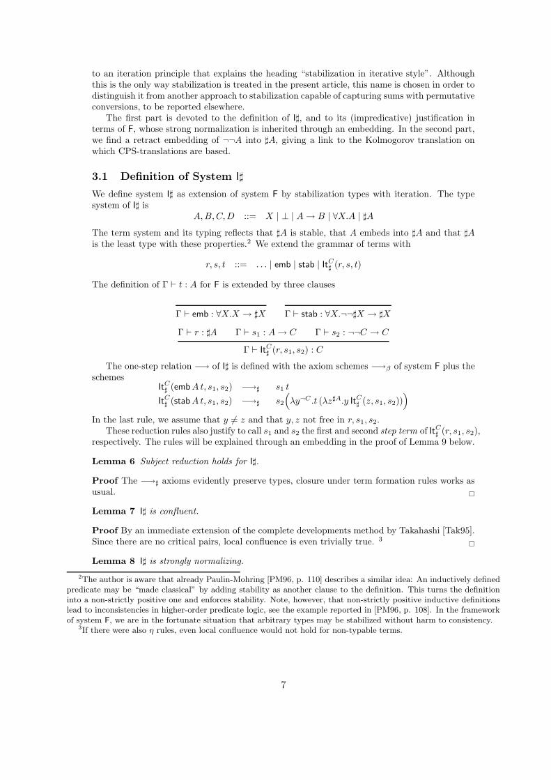
We define system I] as extension of system F by stabilization types with iteration. The typesystem of I] is

A, B, C, D ::= X | ⊥ | A → B | ∀X.A | ]A

The term system and its typing reflects that ]A is stable, that A embeds into ]A and that ]Ais the least type with these properties.2 We extend the grammar of terms with

r, s, t ::= . . . | emb | stab | ItC] (r, s, t)

The definition of Γ ` t : A for F is extended by three clauses

Γ ` emb : ∀X.X → ]X Γ ` stab : ∀X.¬¬]X → ]X

Γ ` r : ]A Γ ` s1 : A → C Γ ` s2 : ¬¬C → C

Γ ` ItC] (r, s1, s2) : C

The one-step relation −→ of I] is defined with the axiom schemes −→β of system F plus theschemes

ItC] (emb A t, s1, s2) −→] s1 t

ItC] (stab A t, s1, s2) −→] s2

(

λy¬C .t (λz]A.y ItC] (z, s1, s2)))

In the last rule, we assume that y 6= z and that y, z not free in r, s1, s2.These reduction rules also justify to call s1 and s2 the first and second step term of ItC] (r, s1, s2),

respectively. The rules will be explained through an embedding in the proof of Lemma 9 below.

Lemma 6 Subject reduction holds for I].

Proof The −→] axioms evidently preserve types, closure under term formation rules works asusual. �

Lemma 7 I] is confluent.

Proof By an immediate extension of the complete developments method by Takahashi [Tak95].Since there are no critical pairs, local confluence is even trivially true. 3

�

Lemma 8 I] is strongly normalizing.

2The author is aware that already Paulin-Mohring [PM96, p. 110] describes a similar idea: An inductively definedpredicate may be “made classical” by adding stability as another clause to the definition. This turns the definitioninto a non-strictly positive one and enforces stability. Note, however, that non-strictly positive inductive definitionslead to inconsistencies in higher-order predicate logic, see the example reported in [PM96, p. 108]. In the frameworkof system F, we are in the fortunate situation that arbitrary types may be stabilized without harm to consistency.

3If there were also η rules, even local confluence would not hold for non-typable terms.

7

The proof will occupy the remainder of this section.The idea of the proof is as follows: Although the second rule for −→] looks unfamiliar, it is

just an instance of iteration over a non-strictly positive inductive type, and hence the reductionbehaviour can be simulated within F.

Definition 1 A type-respecting reduction-preserving embedding (embedding for short) of a termrewrite system S with typing into a term rewrite system S ′ with typing is a function −′ (the −sign represents the indefinite argument of the function ′) which assigns to every type A of S atype A′ of S ′ and to every term r of S a term r′ of S ′ such that the following implications hold:

• If x1 : A1, . . . , xn : An ` r : A in S then x1 : A′1, . . . , xn : A′

n ` r′ : A′ in S ′.

• If r −→ s in S, then r′ −→+ s′ in S ′.

Obviously, if there is an embedding of S into S ′, then strong normalization of S ′ is inherited byS. In the sequel, we will write Γ′ for x1 : A′

1, . . . , xn : A′n if Γ is x1 : A1, . . . , xn : An.

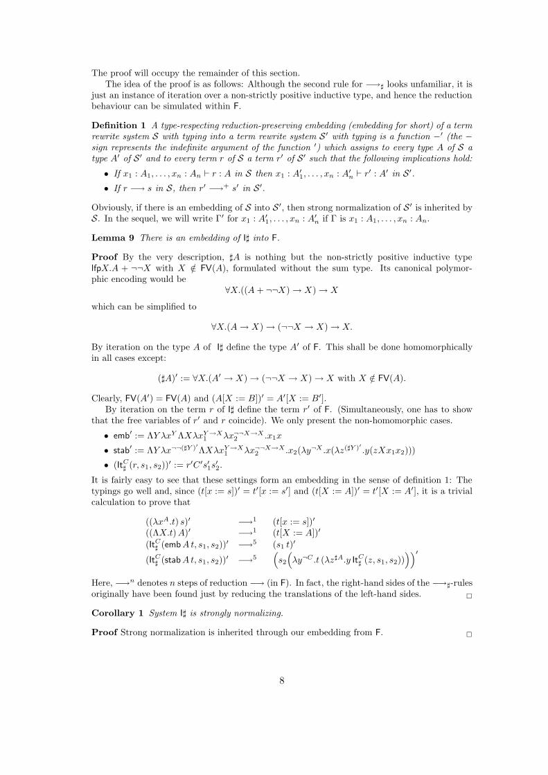
Lemma 9 There is an embedding of I] into F.

Proof By the very description, ]A is nothing but the non-strictly positive inductive typelfpX.A + ¬¬X with X /∈ FV(A), formulated without the sum type. Its canonical polymor-phic encoding would be

∀X.((A + ¬¬X) → X) → X

which can be simplified to

∀X.(A → X) → (¬¬X → X) → X.

By iteration on the type A of I] define the type A′ of F. This shall be done homomorphicallyin all cases except:

(]A)′ := ∀X.(A′ → X) → (¬¬X → X) → X with X /∈ FV(A).

Clearly, FV(A′) = FV(A) and (A[X := B])′ = A′[X := B′].By iteration on the term r of I] define the term r′ of F. (Simultaneously, one has to show

that the free variables of r′ and r coincide). We only present the non-homomorphic cases.

• emb′ := ΛY λxY ΛXλxY →X1 λx¬¬X→X

2 .x1x

• stab′ := ΛY λx¬¬(]Y )′ΛXλxY →X

1 λx¬¬X→X2 .x2(λy¬X .x(λz(]Y )′ .y(zXx1x2)))

• (ItC] (r, s1, s2))′ := r′C ′s′1s

′2.

It is fairly easy to see that these settings form an embedding in the sense of definition 1: Thetypings go well and, since (t[x := s])′ = t′[x := s′] and (t[X := A])′ = t′[X := A′], it is a trivialcalculation to prove that

((λxA.t) s)′ −→1 (t[x := s])′

((ΛX.t) A)′ −→1 (t[X := A])′

(ItC] (emb A t, s1, s2))′ −→5 (s1 t)′

(ItC] (stab A t, s1, s2))′ −→5(

s2

(

λy¬C .t (λz]A.y ItC] (z, s1, s2))))′

Here, −→n denotes n steps of reduction −→ (in F). In fact, the right-hand sides of the −→]-rulesoriginally have been found just by reducing the translations of the left-hand sides. �

Corollary 1 System I] is strongly normalizing.

Proof Strong normalization is inherited through our embedding from F. �

8

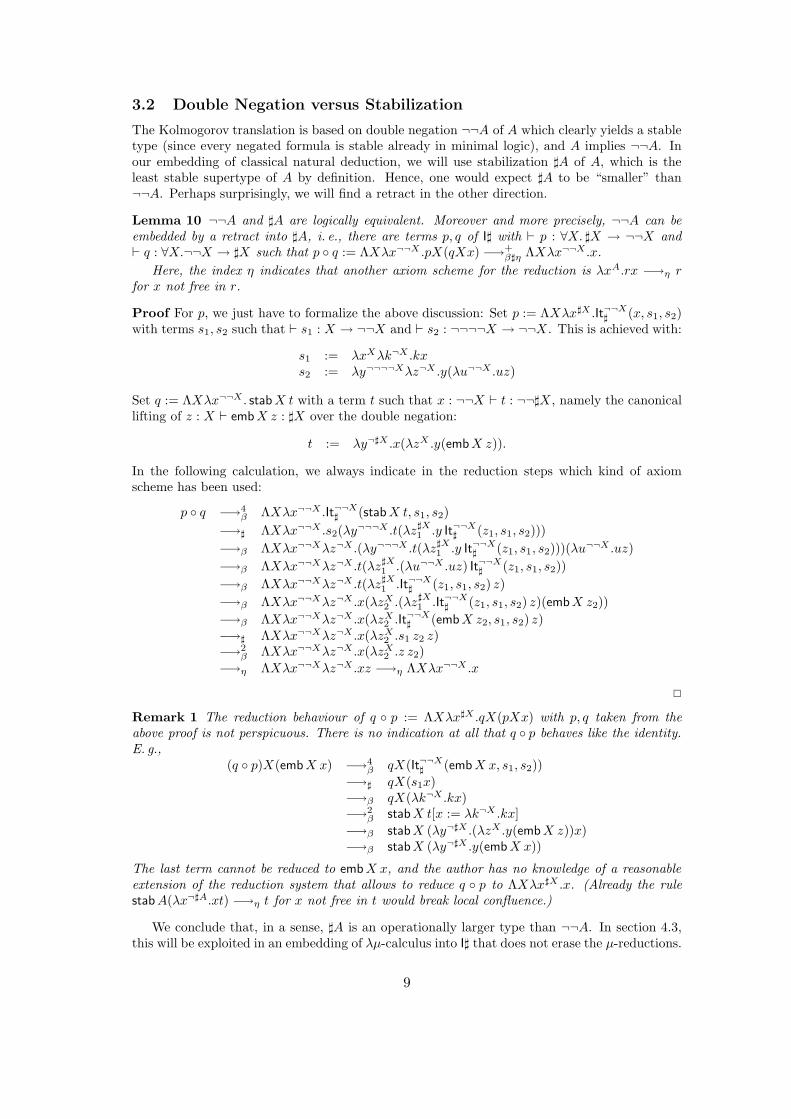
3.2 Double Negation versus Stabilization

The Kolmogorov translation is based on double negation ¬¬A of A which clearly yields a stabletype (since every negated formula is stable already in minimal logic), and A implies ¬¬A. Inour embedding of classical natural deduction, we will use stabilization ]A of A, which is theleast stable supertype of A by definition. Hence, one would expect ]A to be “smaller” than¬¬A. Perhaps surprisingly, we will find a retract in the other direction.

Lemma 10 ¬¬A and ]A are logically equivalent. Moreover and more precisely, ¬¬A can beembedded by a retract into ]A, i. e., there are terms p, q of I] with ` p : ∀X. ]X → ¬¬X and` q : ∀X.¬¬X → ]X such that p ◦ q := ΛXλx¬¬X .pX(qXx) −→+

β]η ΛXλx¬¬X .x.

Here, the index η indicates that another axiom scheme for the reduction is λxA.rx −→η rfor x not free in r.

Proof For p, we just have to formalize the above discussion: Set p := ΛXλx]X .It¬¬X] (x, s1, s2)

with terms s1, s2 such that ` s1 : X → ¬¬X and ` s2 : ¬¬¬¬X → ¬¬X . This is achieved with:

s1 := λxXλk¬X .kxs2 := λy¬¬¬¬Xλz¬X .y(λu¬¬X .uz)

Set q := ΛXλx¬¬X . stab X t with a term t such that x : ¬¬X ` t : ¬¬]X , namely the canonicallifting of z : X ` embX z : ]X over the double negation:

t := λy¬]X .x(λzX .y(embX z)).

In the following calculation, we always indicate in the reduction steps which kind of axiomscheme has been used:

p ◦ q −→4β ΛXλx¬¬X .It¬¬X

] (stab X t, s1, s2)

−→] ΛXλx¬¬X .s2(λy¬¬¬X .t(λz]X1 .y It¬¬X

] (z1, s1, s2)))

−→β ΛXλx¬¬Xλz¬X .(λy¬¬¬X .t(λz]X1 .y It¬¬X

] (z1, s1, s2)))(λu¬¬X .uz)

−→β ΛXλx¬¬Xλz¬X .t(λz]X1 .(λu¬¬X .uz) It¬¬X

] (z1, s1, s2))

−→β ΛXλx¬¬Xλz¬X .t(λz]X1 .It¬¬X

] (z1, s1, s2) z)

−→β ΛXλx¬¬Xλz¬X .x(λzX2 .(λz]X

1 .It¬¬X] (z1, s1, s2) z)(embX z2))

−→β ΛXλx¬¬Xλz¬X .x(λzX2 .It¬¬X

] (emb X z2, s1, s2) z)−→] ΛXλx¬¬Xλz¬X .x(λzX

2 .s1 z2 z)−→2

β ΛXλx¬¬Xλz¬X .x(λzX2 .z z2)

−→η ΛXλx¬¬Xλz¬X .xz −→η ΛXλx¬¬X .x

�

Remark 1 The reduction behaviour of q ◦ p := ΛXλx]X .qX(pXx) with p, q taken from theabove proof is not perspicuous. There is no indication at all that q ◦ p behaves like the identity.E. g.,

(q ◦ p)X(embX x) −→4β qX(It¬¬X

] (emb X x, s1, s2))

−→] qX(s1x)−→β qX(λk¬X .kx)−→2

β stabX t[x := λk¬X .kx]

−→β stabX (λy¬]X .(λzX .y(emb X z))x)−→β stabX (λy¬]X .y(emb X x))

The last term cannot be reduced to emb X x, and the author has no knowledge of a reasonableextension of the reduction system that allows to reduce q ◦ p to ΛXλx]X .x. (Already the rulestab A(λx¬]A.xt) −→η t for x not free in t would break local confluence.)

We conclude that, in a sense, ]A is an operationally larger type than ¬¬A. In section 4.3,this will be exploited in an embedding of λµ-calculus into I] that does not erase the µ-reductions.

9

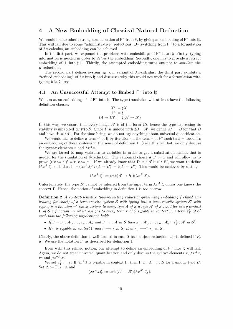
4 A New Embedding of Classical Natural Deduction

We would like to inherit strong normalization of F¬ from F, by giving an embedding of F¬ into I].This will fail due to some “administrative” reductions. By switching from F¬ to a formulationof λµ-calculus, an embedding can be achieved.

In the first part, we expound the problems with embeddings of F¬ into I]: Firstly, typinginformation is needed in order to define the embedding. Secondly, one has to provide a retractembedding of ⊥ into ]⊥. Thirdly, the attempted embedding turns out not to simulate theµ-reductions.

The second part defines system λµ, our variant of λµ-calculus, the third part exhibits a“refined embedding” of λµ into I] and discusses why this would not work for a formulation withtyping a la Curry.

4.1 An Unsuccessful Attempt to Embed F¬ into I]

We aim at an embedding −′ of F¬ into I]. The type translation will at least have the followingdefinition clauses:

X ′ := ]X⊥′ := ]⊥

(A → B)′ := ](A′ → B′)

In this way, we ensure that every image A′ is of the form ]B, hence the type expressing itsstability is inhabited by stabB. Since B is unique with ]B = A′, we define A∗ := B for that Band have A′ = ]A∗. For the time being, we do not say anything about universal quantification.

We would like to define a term r′ of I] by iteration on the term r of F¬ such that −′ becomesan embedding of these systems in the sense of definition 1. Since this will fail, we only discussthe syntax elements x and λxA.t.

We are forced to map variables to variables in order to get a substitution lemma that isneeded for the simulation of β-reduction. The canonical choice is x′ := x and will allow us toprove (t[x := s])′ = t′[x := s′]. If we already know that Γ′, x : A′ ` t′ : B′, we want to define(λxA.t)′ such that Γ′ ` (λxA.t)′ : (A → B)′ = ](A′ → B′). This would be achieved by setting

(λxA.t)′ := emb(A′ → B′)(λxA′

.t′).

Unfortunately, the type B′ cannot be inferred from the input term λxA.t, unless one knows thecontext Γ. Hence, the notion of embedding in definition 1 is too narrow.

Definition 2 A context-sensitive type-respecting reduction-preserving embedding (refined em-bedding for short) of a term rewrite system S with typing into a term rewrite system S ′ withtyping is a function −′ which assigns to every type A of S a type A′ of S ′, and for every contextΓ of S a function −′

Γ which assigns to every term r of S typable in context Γ, a term r′Γ of S ′

such that the following implications hold:

• If Γ = x1 : A1, . . . , xn : An and Γ ` r : A in S then x1 : A′1, . . . , xn : A′

n ` r′Γ : A′ in S ′.

• If r is typable in context Γ and r −→ s in S, then r′Γ −→+ s′Γ in S ′.

Clearly, the above definition is well-formed in case S has subject reduction: s′Γ is defined if r′Γis. We use the notation Γ′ as described for definition 1.

Even with this refined notion, our attempt to define an embedding of F¬ into I] will fail.Again, we do not treat universal quantification and only discuss the syntax elements x, λxA.t,rs and µx¬A.r.

We set x′Γ := x. If λxA.t is typable in context Γ, then Γ, x : A ` t : B for a unique type B.

Set ∆ := Γ, x : A and(λxA.t)′Γ := emb(A′ → B′)(λxA′

.t′∆).

10

In a proof that this definition respects types (the first condition in the definition), one wouldhave Γ′, x : A′ ` t′∆ : B′ by induction hypothesis, hence Γ′ ` (λxA.t)′Γ : (A → B)′.

With the (inductive) assumptions Γ′ ` r′Γ : (A → B)′ = ](A′ → B′) and Γ′ ` s′Γ : A′ inmind, we set

(rs)′Γ := ItB′

] (r′Γ, λzA′→B′

.zs′Γ, stabB∗)

with z not free in s. Since Γ′ ` λzA′→B′

.zs′Γ : (A′ → B′) → B′ and Γ′ ` stab B∗ : ¬¬B′ → B′,we get Γ′ ` (rs)′Γ : B′. The definition is well-formed since A and B are uniquely determined byΓ and r: The type A → B is the unique type of r in context Γ.

The crucial case is as follows: Setting ∆ := Γ, x : ¬A, we may assume that Γ′, x : (¬A)′ `r′∆ : ⊥′ and want to define (µx¬A.r)′Γ such that Γ′ ` (µx¬A.r)′Γ : A′. Unfolding the definitions,our assumption reads Γ′, x : ](A′ → ]⊥) ` r′∆ : ]⊥. First, we need to go back and forth between]⊥ and ⊥:

Lemma 11 The type ⊥ can be embedded by a retract into ]⊥, i. e., there are terms p, q with` p : ]⊥ → ⊥ and ` q : ⊥ → ]⊥ such that p(qx) −→+ x. (Note that we do not even need ηreductions here.)

Proof Set q := emb⊥ and p := λx]⊥.It⊥] (x, id⊥, λz¬¬⊥.z id⊥). Calculate p(qx) = p(emb⊥x) −→2

id⊥ x −→ x. �

With these terms p, q we define q ◦A y := λzA′

.q(yz) (think of y : ¬A′ in the context, henceq ◦A y : A′ → ]⊥) and

(µx¬A.r)′Γ := stabA∗

(

λy¬A′

.p(

r′∆[x := emb(A′ → ]⊥)(q ◦A y)]))

.

This is type-correct since, we have y : ¬A′ ` emb(A′ → ]⊥)(q ◦A y) : ](A′ → ]⊥), henceΓ′, y : ¬A′ ` r′∆[x := emb(A′ → ]⊥)(q ◦A y)] : ]⊥ by the cut rule, finally, Γ′ ` λy¬A′

.p(r′∆[x :=emb(A′ → ]⊥)(q ◦A y)]) : ¬¬A′.

For the syntax captured by these definitions, we can prove that weakening and cut also holdfor the prospective embedding, in the following sense:

• If Γ ` t : B and x is not declared in Γ, then t′Γ = t′Γ,x:A.

• If Γ, x : A ` t : B and Γ ` s : A then (t[x := s])′Γ = t′Γ,x:A[x := s′Γ].

Although ordinary β-reduction would be simulated, we demonstrate that, for (µx¬(A→B).r)stypable in Γ, we do not have

L := ((µx¬(A→B).r)s)′Γ −→+ (µy¬B .r[x := λzA→B .y(zs)])′Γ =: R

Abbreviate emb(A′ → ]⊥) by eA and set ∆ := Γ, x : ¬(A → B).

L = ItB′

]

(

stab(A → B)∗(

λy¬(A→B)′ .p(r′∆[x := eA→B(q ◦A→B y)]))

, λzA′→B′

.zs′Γ, stabB∗

)

−→] stabB∗

(

λy¬B′

.(

λy¬(A→B)′ .p(r′∆[x := eA→B(q ◦A→B y)]))

(λz(A→B)′ .y(zs)′Γ,z:A→B))

−→β stabB∗

(

λy¬B′

.p(

r′∆

[

x := eA→B(

λz(A→B)′ .q(

(λz(A→B)′ .y(zs)′Γ,z:A→B)z))]))

−→∗ stabB∗

(

λy¬B′

.p(

r′∆

[

x := eA→B(

λz(A→B)′ .q(y(zs)′Γ,z:A→B))]))

=: L+

R = stabB∗

(

λy¬B′

.p(

r′∆[x := (λzA→B .y(zs))′Γ,y:¬B︸ ︷︷ ︸

eA→B(λz(A→B)′ .(y(zs))′Γ,y:¬B,z:A→B)

][y := eB(q ◦B y)]))

= stabB∗

(

λy¬B′

.p(

r′∆

[

x := eA→B(

λz(A→B)′ .(y(zs))′Γ,y:¬B,z:A→B[y := eB(q ◦B y)])]))

−→∗ L+

This is justified by the following reductions for every occurrence of x in r′∆ (only in case x notfree in r′∆, the desired R = L+ holds true):

(y(zs))′Γ,y:¬B,z:A→B = It]⊥] (y, λuB′

→]⊥.u(zs)′Γ,z:A→B, stab⊥),

11

hence

(y(zs))′Γ,y:¬B,z:A→B[y := eB(q ◦B y)] = It]⊥] (eB(q ◦B y), λuB′

→]⊥.u(zs)′Γ,z:A→B , stab⊥)

−→] (λuB′→]⊥.u(zs)′Γ,z:A→B)(q ◦B y)

−→β (q ◦B y)(zs)′Γ,z:A→B

−→β q(y(zs)′Γ,z:A→B)

The author does not see a way how to infer strong normalization of F¬ from that of I] due tothis failure of simulation. The unwanted “administrative” reductions in R will be avoided if wedo not replace x by λzA→B .y(zs) in the µ-reduction rule, but, loosely speaking, every occurrenceof a subterm of the form x t by y(ts). This will only be a reasonable reduction relation if everyoccurrence of x is in a subterm of that form x t. Certainly, this cannot be expected. But weonly need it for the variables x that are bound by µ. Hence, we introduce two name spaces forvariables, one for the usual variables that may be bound by λ, hence called λ-variables, the otherone for the variables possibly bound by µ, called µ-variables. And only for those µ-variables a,we will ensure that they occur only in a subterm of the form a t. Essentially, this gives Parigot’sλµ-calculus [Par92]. However, like de Groote [dG94], we will not be so strict as to require thatone can only µ-abstract over terms of that form a t. We even allow ⊥ as a type former andhence stay more closely to the more recent presentation by de Groote [dG01].

4.2 Refined Classical Natural Deduction: λµ-Calculus

As mentioned above, Parigot’s second-order typed λµ-calculus will be slightly extended in thestyle of de Groote [dG01]. However, we do not put the typing context for the µ-variables to theright-hand side of `. Moreover, we use raw syntax in Church style.

The system of types of λµ is just that of F (which is the same as that for F¬). The termsystem of F is extended as follows: There is an infinite set of µ-variables, whose elements aredenoted by a, b, c. They are supposed to be disjoint from the variables x, now called λ-variables.The additional formation rules for terms in λµ are

r, s, t ::= . . . | a t | µaA.r

Hence, a µ-variable alone is no term, and every variable that will ever get bound by µ onlyoccurs as left-hand side a of an application a t.

The contexts may also contain pairs (a : A) of µ-variables and types, to be interpreted as ahaving type ¬A.

In addition to the typing rules of F, we have the rules involving the µ-variables

Γ, a : A ` t : A

Γ, a : A ` a t : ⊥

Γ, a : A ` r : ⊥

Γ ` µaA.r : A

Although a µ-variable is not a term, it can be turned into a term of the appropriate type: Wehave a : A ` λxA. a x : ¬A.

The axiom schemes for −→β are taken from F. −→µ of F¬ is changed to a rule that nolonger has a lambda abstraction in the right-hand side. We need a special form of substitutionwhich is called structural substitution by de Groote [dG01].

Definition 3 A term context is derived from a term by replacing exactly one occurrence of aλ-variable in that term with the new symbol ?. This occurrence must not be in the scope of anybinder (for simplicity). Term contexts will be communicated by the letter E, and the result of atextual substitution of a term r for ? in E, will be denoted by E[r] (and is a term).

Definition 4 (Special Substitution) For r a term, µ-variables a, b and a term context E,define the term r[a ? := b E] as the result of replacing in r recursively every subterm of the form

12

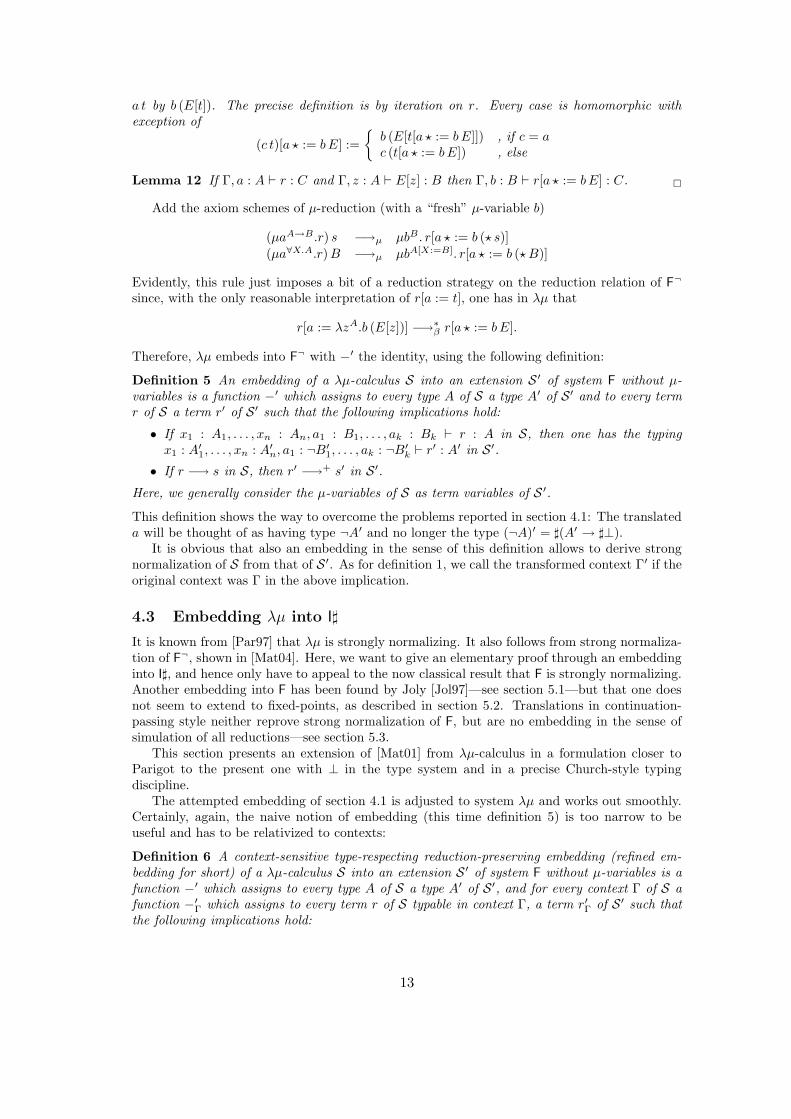
a t by b (E[t]). The precise definition is by iteration on r. Every case is homomorphic withexception of

(c t)[a ? := b E] :=

{b (E[t[a ? := b E]]) , if c = ac (t[a ? := b E]) , else

Lemma 12 If Γ, a : A ` r : C and Γ, z : A ` E[z] : B then Γ, b : B ` r[a ? := b E] : C. �

Add the axiom schemes of µ-reduction (with a “fresh” µ-variable b)

(µaA→B .r) s −→µ µbB . r[a ? := b (? s)]

(µa∀X.A.r) B −→µ µbA[X:=B]. r[a ? := b (? B)]

Evidently, this rule just imposes a bit of a reduction strategy on the reduction relation of F¬

since, with the only reasonable interpretation of r[a := t], one has in λµ that

r[a := λzA.b (E[z])] −→∗β r[a ? := b E].

Therefore, λµ embeds into F¬ with −′ the identity, using the following definition:

Definition 5 An embedding of a λµ-calculus S into an extension S ′ of system F without µ-variables is a function −′ which assigns to every type A of S a type A′ of S ′ and to every termr of S a term r′ of S ′ such that the following implications hold:

• If x1 : A1, . . . , xn : An, a1 : B1, . . . , ak : Bk ` r : A in S, then one has the typingx1 : A′

1, . . . , xn : A′n, a1 : ¬B′

1, . . . , ak : ¬B′k ` r′ : A′ in S ′.

• If r −→ s in S, then r′ −→+ s′ in S ′.

Here, we generally consider the µ-variables of S as term variables of S ′.

This definition shows the way to overcome the problems reported in section 4.1: The translateda will be thought of as having type ¬A′ and no longer the type (¬A)′ = ](A′ → ]⊥).

It is obvious that also an embedding in the sense of this definition allows to derive strongnormalization of S from that of S ′. As for definition 1, we call the transformed context Γ′ if theoriginal context was Γ in the above implication.

4.3 Embedding λµ into I]

It is known from [Par97] that λµ is strongly normalizing. It also follows from strong normaliza-tion of F¬, shown in [Mat04]. Here, we want to give an elementary proof through an embeddinginto I], and hence only have to appeal to the now classical result that F is strongly normalizing.Another embedding into F has been found by Joly [Jol97]—see section 5.1—but that one doesnot seem to extend to fixed-points, as described in section 5.2. Translations in continuation-passing style neither reprove strong normalization of F, but are no embedding in the sense ofsimulation of all reductions—see section 5.3.

This section presents an extension of [Mat01] from λµ-calculus in a formulation closer toParigot to the present one with ⊥ in the type system and in a precise Church-style typingdiscipline.

The attempted embedding of section 4.1 is adjusted to system λµ and works out smoothly.Certainly, again, the naive notion of embedding (this time definition 5) is too narrow to beuseful and has to be relativized to contexts:

Definition 6 A context-sensitive type-respecting reduction-preserving embedding (refined em-bedding for short) of a λµ-calculus S into an extension S ′ of system F without µ-variables is afunction −′ which assigns to every type A of S a type A′ of S ′, and for every context Γ of S afunction −′

Γ which assigns to every term r of S typable in context Γ, a term r′Γ of S ′ such thatthe following implications hold:

13

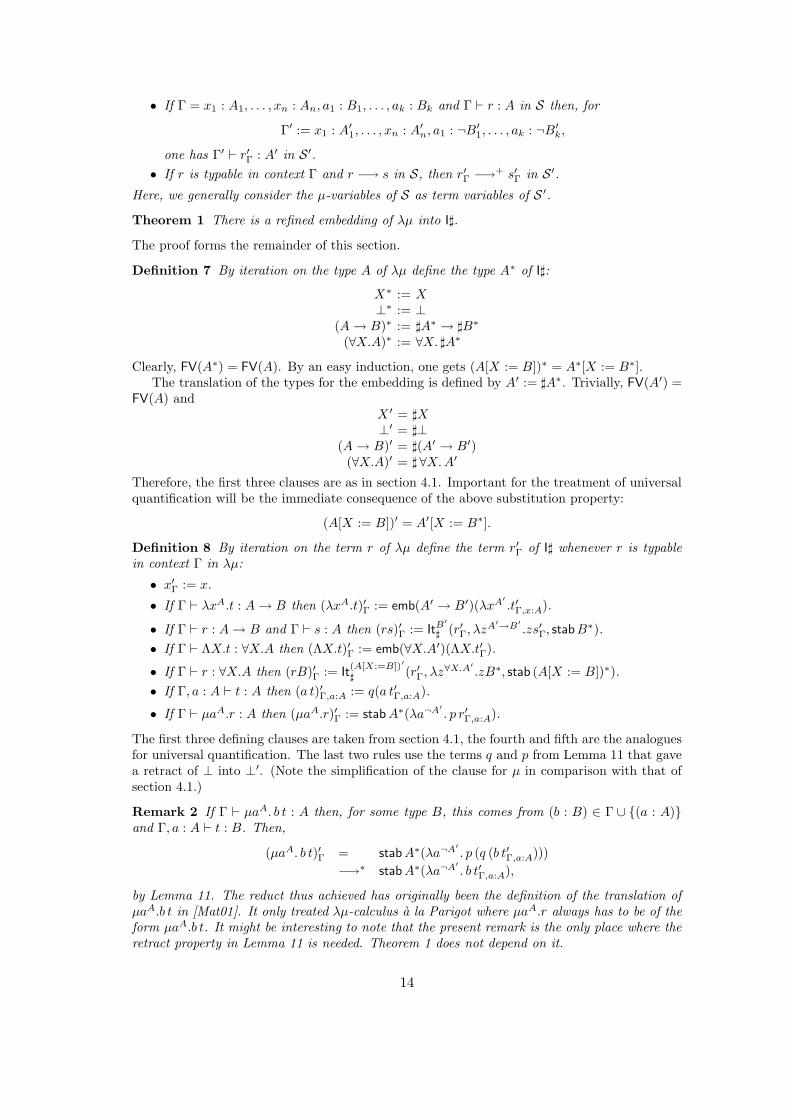
• If Γ = x1 : A1, . . . , xn : An, a1 : B1, . . . , ak : Bk and Γ ` r : A in S then, for

Γ′ := x1 : A′1, . . . , xn : A′

n, a1 : ¬B′1, . . . , ak : ¬B′

k,

one has Γ′ ` r′Γ : A′ in S ′.

• If r is typable in context Γ and r −→ s in S, then r′Γ −→+ s′Γ in S ′.

Here, we generally consider the µ-variables of S as term variables of S ′.

Theorem 1 There is a refined embedding of λµ into I].

The proof forms the remainder of this section.

Definition 7 By iteration on the type A of λµ define the type A∗ of I]:

X∗ := X⊥∗ := ⊥

(A → B)∗ := ]A∗ → ]B∗

(∀X.A)∗ := ∀X. ]A∗

Clearly, FV(A∗) = FV(A). By an easy induction, one gets (A[X := B])∗ = A∗[X := B∗].The translation of the types for the embedding is defined by A′ := ]A∗. Trivially, FV(A′) =

FV(A) andX ′ = ]X⊥′ = ]⊥

(A → B)′ = ](A′ → B′)(∀X.A)′ = ] ∀X. A′

Therefore, the first three clauses are as in section 4.1. Important for the treatment of universalquantification will be the immediate consequence of the above substitution property:

(A[X := B])′ = A′[X := B∗].

Definition 8 By iteration on the term r of λµ define the term r′Γ of I] whenever r is typablein context Γ in λµ:

• x′Γ := x.

• If Γ ` λxA.t : A → B then (λxA.t)′Γ := emb(A′ → B′)(λxA′

.t′Γ,x:A).

• If Γ ` r : A → B and Γ ` s : A then (rs)′Γ := ItB′

] (r′Γ, λzA′→B′

.zs′Γ, stabB∗).

• If Γ ` ΛX.t : ∀X.A then (ΛX.t)′Γ := emb(∀X.A′)(ΛX.t′Γ).

• If Γ ` r : ∀X.A then (rB)′Γ := It(A[X:=B])′

] (r′Γ, λz∀X.A′

.zB∗, stab (A[X := B])∗).

• If Γ, a : A ` t : A then (a t)′Γ,a:A := q(a t′Γ,a:A).

• If Γ ` µaA.r : A then (µaA.r)′Γ := stab A∗(λa¬A′

. p r′Γ,a:A).

The first three defining clauses are taken from section 4.1, the fourth and fifth are the analoguesfor universal quantification. The last two rules use the terms q and p from Lemma 11 that gavea retract of ⊥ into ⊥′. (Note the simplification of the clause for µ in comparison with that ofsection 4.1.)

Remark 2 If Γ ` µaA. b t : A then, for some type B, this comes from (b : B) ∈ Γ ∪ {(a : A)}and Γ, a : A ` t : B. Then,

(µaA. b t)′Γ = stab A∗(λa¬A′

. p (q (b t′Γ,a:A)))

−→∗ stab A∗(λa¬A′

. b t′Γ,a:A),

by Lemma 11. The reduct thus achieved has originally been the definition of the translation ofµaA.b t in [Mat01]. It only treated λµ-calculus a la Parigot where µaA.r always has to be of theform µaA.b t. It might be interesting to note that the present remark is the only place where theretract property in Lemma 11 is needed. Theorem 1 does not depend on it.

14

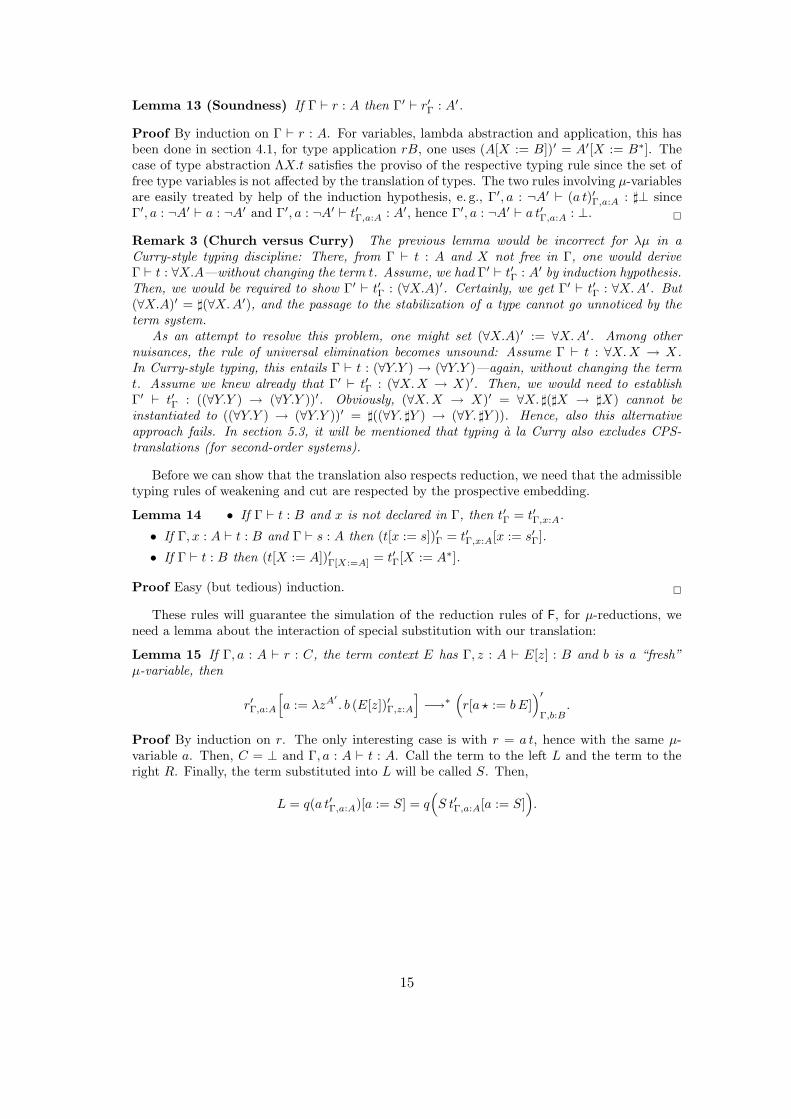
Lemma 13 (Soundness) If Γ ` r : A then Γ′ ` r′Γ : A′.

Proof By induction on Γ ` r : A. For variables, lambda abstraction and application, this hasbeen done in section 4.1, for type application rB, one uses (A[X := B])′ = A′[X := B∗]. Thecase of type abstraction ΛX.t satisfies the proviso of the respective typing rule since the set offree type variables is not affected by the translation of types. The two rules involving µ-variablesare easily treated by help of the induction hypothesis, e. g., Γ′, a : ¬A′ ` (a t)′Γ,a:A : ]⊥ sinceΓ′, a : ¬A′ ` a : ¬A′ and Γ′, a : ¬A′ ` t′Γ,a:A : A′, hence Γ′, a : ¬A′ ` a t′Γ,a:A : ⊥. �

Remark 3 (Church versus Curry) The previous lemma would be incorrect for λµ in aCurry-style typing discipline: There, from Γ ` t : A and X not free in Γ, one would deriveΓ ` t : ∀X.A—without changing the term t. Assume, we had Γ′ ` t′Γ : A′ by induction hypothesis.Then, we would be required to show Γ′ ` t′Γ : (∀X.A)′. Certainly, we get Γ′ ` t′Γ : ∀X. A′. But(∀X.A)′ = ](∀X. A′), and the passage to the stabilization of a type cannot go unnoticed by theterm system.

As an attempt to resolve this problem, one might set (∀X.A)′ := ∀X. A′. Among othernuisances, the rule of universal elimination becomes unsound: Assume Γ ` t : ∀X. X → X.In Curry-style typing, this entails Γ ` t : (∀Y.Y ) → (∀Y.Y )—again, without changing the termt. Assume we knew already that Γ′ ` t′Γ : (∀X. X → X)′. Then, we would need to establishΓ′ ` t′Γ : ((∀Y.Y ) → (∀Y.Y ))′. Obviously, (∀X. X → X)′ = ∀X. ](]X → ]X) cannot beinstantiated to ((∀Y.Y ) → (∀Y.Y ))′ = ]((∀Y. ]Y ) → (∀Y. ]Y )). Hence, also this alternativeapproach fails. In section 5.3, it will be mentioned that typing a la Curry also excludes CPS-translations (for second-order systems).

Before we can show that the translation also respects reduction, we need that the admissibletyping rules of weakening and cut are respected by the prospective embedding.

Lemma 14 • If Γ ` t : B and x is not declared in Γ, then t′Γ = t′Γ,x:A.

• If Γ, x : A ` t : B and Γ ` s : A then (t[x := s])′Γ = t′Γ,x:A[x := s′Γ].

• If Γ ` t : B then (t[X := A])′Γ[X:=A] = t′Γ[X := A∗].

Proof Easy (but tedious) induction. �

These rules will guarantee the simulation of the reduction rules of F, for µ-reductions, weneed a lemma about the interaction of special substitution with our translation:

Lemma 15 If Γ, a : A ` r : C, the term context E has Γ, z : A ` E[z] : B and b is a “fresh”µ-variable, then

r′Γ,a:A

[

a := λzA′

. b (E[z])′Γ,z:A

]

−→∗

(

r[a ? := b E])′

Γ,b:B.

Proof By induction on r. The only interesting case is with r = a t, hence with the same µ-variable a. Then, C = ⊥ and Γ, a : A ` t : A. Call the term to the left L and the term to theright R. Finally, the term substituted into L will be called S. Then,

L = q(a t′Γ,a:A)[a := S] = q(

S t′Γ,a:A[a := S])

.

15

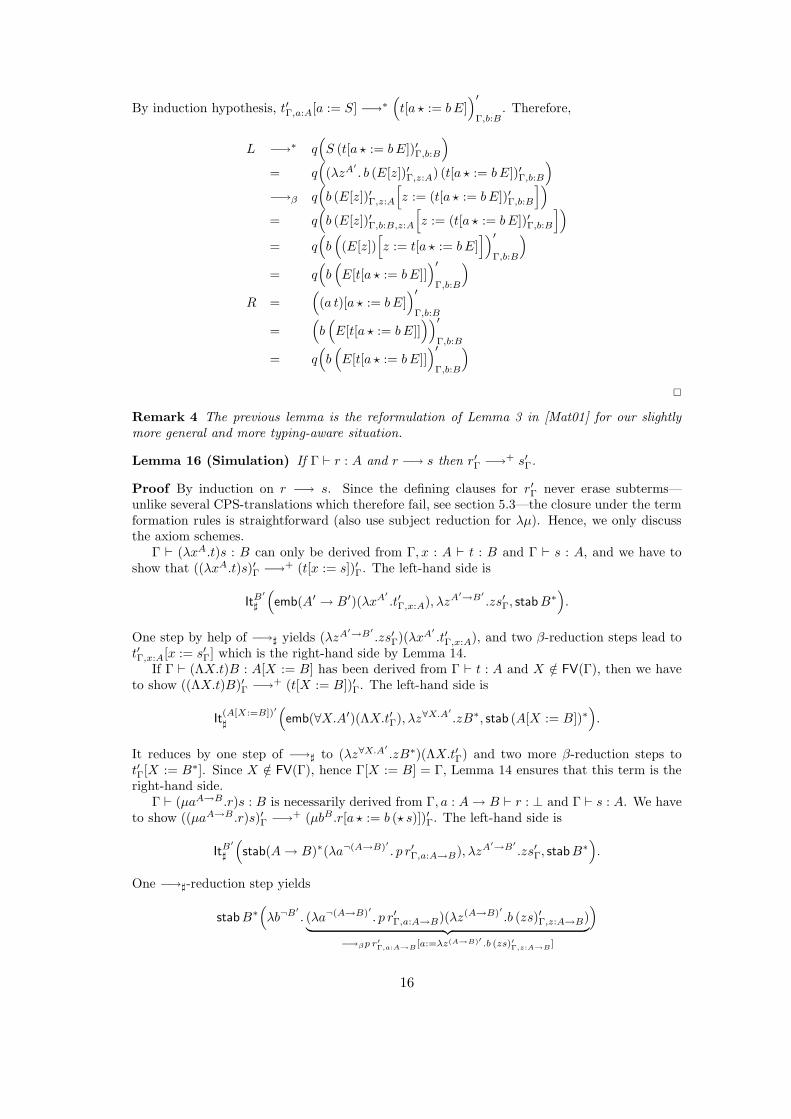
By induction hypothesis, t′Γ,a:A[a := S] −→∗

(

t[a ? := b E])′

Γ,b:B. Therefore,

L −→∗ q(

S (t[a ? := b E])′Γ,b:B

)

= q(

(λzA′

. b (E[z])′Γ,z:A) (t[a ? := b E])′Γ,b:B

)

−→β q(

b (E[z])′Γ,z:A

[

z := (t[a ? := b E])′Γ,b:B

])

= q(

b (E[z])′Γ,b:B,z:A

[

z := (t[a ? := b E])′Γ,b:B

])

= q(

b(

(E[z])[

z := t[a ? := b E]])′

Γ,b:B

)

= q(

b(

E[t[a ? := b E]])′

Γ,b:B

)

R =(

(a t)[a ? := b E])′

Γ,b:B

=(

b(

E[t[a ? := b E]]))′

Γ,b:B

= q(

b(

E[t[a ? := b E]])′

Γ,b:B

)

�

Remark 4 The previous lemma is the reformulation of Lemma 3 in [Mat01] for our slightlymore general and more typing-aware situation.

Lemma 16 (Simulation) If Γ ` r : A and r −→ s then r′Γ −→+ s′Γ.

Proof By induction on r −→ s. Since the defining clauses for r′Γ never erase subterms—unlike several CPS-translations which therefore fail, see section 5.3—the closure under the termformation rules is straightforward (also use subject reduction for λµ). Hence, we only discussthe axiom schemes.

Γ ` (λxA.t)s : B can only be derived from Γ, x : A ` t : B and Γ ` s : A, and we have toshow that ((λxA.t)s)′Γ −→+ (t[x := s])′Γ. The left-hand side is

ItB′

]

(

emb(A′ → B′)(λxA′

.t′Γ,x:A), λzA′→B′

.zs′Γ, stab B∗

)

.

One step by help of −→] yields (λzA′→B′

.zs′Γ)(λxA′

.t′Γ,x:A), and two β-reduction steps lead tot′Γ,x:A[x := s′Γ] which is the right-hand side by Lemma 14.

If Γ ` (ΛX.t)B : A[X := B] has been derived from Γ ` t : A and X /∈ FV(Γ), then we haveto show ((ΛX.t)B)′Γ −→+ (t[X := B])′Γ. The left-hand side is

It(A[X:=B])′

]

(

emb(∀X.A′)(ΛX.t′Γ), λz∀X.A′

.zB∗, stab (A[X := B])∗)

.

It reduces by one step of −→] to (λz∀X.A′

.zB∗)(ΛX.t′Γ) and two more β-reduction steps tot′Γ[X := B∗]. Since X /∈ FV(Γ), hence Γ[X := B] = Γ, Lemma 14 ensures that this term is theright-hand side.

Γ ` (µaA→B .r)s : B is necessarily derived from Γ, a : A → B ` r : ⊥ and Γ ` s : A. We haveto show ((µaA→B .r)s)′Γ −→+ (µbB .r[a ? := b (? s)])′Γ. The left-hand side is

ItB′

]

(

stab(A → B)∗(λa¬(A→B)′ . p r′Γ,a:A→B), λzA′→B′

.zs′Γ, stabB∗

)

.

One −→]-reduction step yields

stabB∗

(

λb¬B′

. (λa¬(A→B)′ . p r′Γ,a:A→B)(λz(A→B)′ .b (zs)′Γ,z:A→B)︸ ︷︷ ︸

−→βp r′

Γ,a:A→B[a:=λz(A→B)′ .b (zs)′Γ,z:A→B

]

)

16

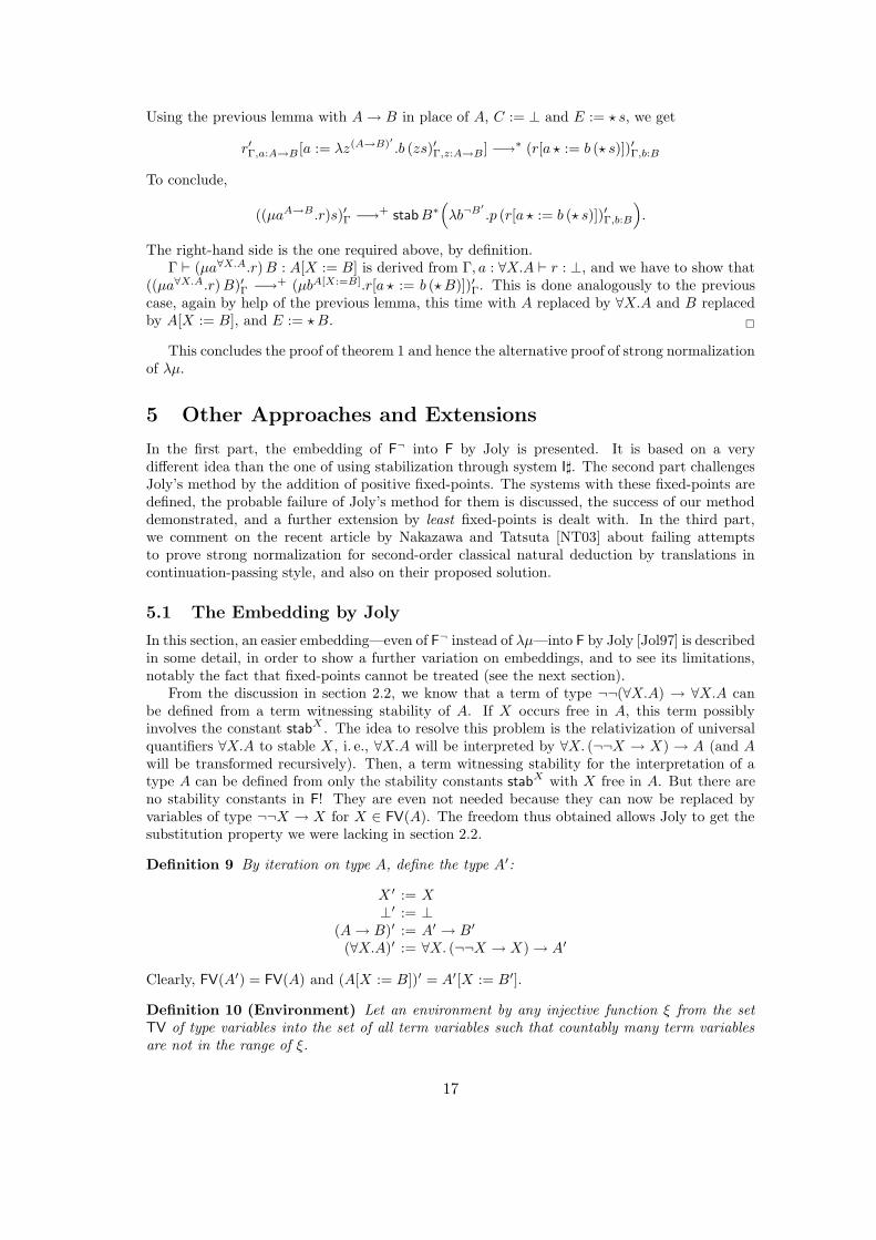
Using the previous lemma with A → B in place of A, C := ⊥ and E := ? s, we get

r′Γ,a:A→B [a := λz(A→B)′ .b (zs)′Γ,z:A→B] −→∗ (r[a ? := b (? s)])′Γ,b:B

To conclude,

((µaA→B .r)s)′Γ −→+ stabB∗

(

λb¬B′

.p (r[a ? := b (? s)])′Γ,b:B

)

.

The right-hand side is the one required above, by definition.Γ ` (µa∀X.A.r) B : A[X := B] is derived from Γ, a : ∀X.A ` r : ⊥, and we have to show that

((µa∀X.A.r) B)′Γ −→+ (µbA[X:=B].r[a ? := b (? B)])′Γ. This is done analogously to the previouscase, again by help of the previous lemma, this time with A replaced by ∀X.A and B replacedby A[X := B], and E := ? B. �

This concludes the proof of theorem 1 and hence the alternative proof of strong normalizationof λµ.

5 Other Approaches and Extensions

In the first part, the embedding of F¬ into F by Joly is presented. It is based on a verydifferent idea than the one of using stabilization through system I]. The second part challengesJoly’s method by the addition of positive fixed-points. The systems with these fixed-points aredefined, the probable failure of Joly’s method for them is discussed, the success of our methoddemonstrated, and a further extension by least fixed-points is dealt with. In the third part,we comment on the recent article by Nakazawa and Tatsuta [NT03] about failing attemptsto prove strong normalization for second-order classical natural deduction by translations incontinuation-passing style, and also on their proposed solution.

5.1 The Embedding by Joly

In this section, an easier embedding—even of F¬ instead of λµ—into F by Joly [Jol97] is describedin some detail, in order to show a further variation on embeddings, and to see its limitations,notably the fact that fixed-points cannot be treated (see the next section).

From the discussion in section 2.2, we know that a term of type ¬¬(∀X.A) → ∀X.A canbe defined from a term witnessing stability of A. If X occurs free in A, this term possiblyinvolves the constant stabX . The idea to resolve this problem is the relativization of universalquantifiers ∀X.A to stable X , i. e., ∀X.A will be interpreted by ∀X. (¬¬X → X) → A (and Awill be transformed recursively). Then, a term witnessing stability for the interpretation of atype A can be defined from only the stability constants stabX with X free in A. But there areno stability constants in F! They are even not needed because they can now be replaced byvariables of type ¬¬X → X for X ∈ FV(A). The freedom thus obtained allows Joly to get thesubstitution property we were lacking in section 2.2.

Definition 9 By iteration on type A, define the type A′:

X ′ := X⊥′ := ⊥

(A → B)′ := A′ → B′

(∀X.A)′ := ∀X. (¬¬X → X) → A′

Clearly, FV(A′) = FV(A) and (A[X := B])′ = A′[X := B′].

Definition 10 (Environment) Let an environment by any injective function ξ from the setTV of type variables into the set of all term variables such that countably many term variablesare not in the range of ξ.

17

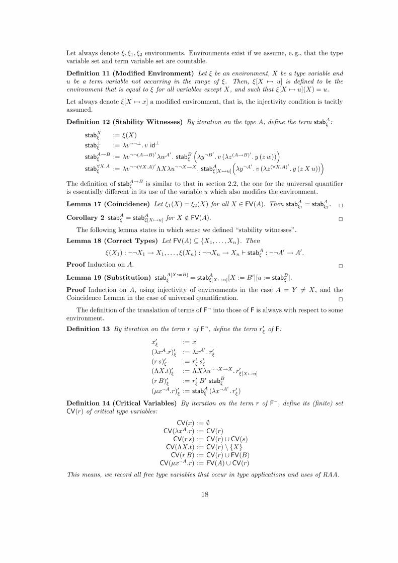
Let always denote ξ, ξ1, ξ2 environments. Environments exist if we assume, e. g., that the typevariable set and term variable set are countable.

Definition 11 (Modified Environment) Let ξ be an environment, X be a type variable andu be a term variable not occurring in the range of ξ. Then, ξ[X 7→ u] is defined to be theenvironment that is equal to ξ for all variables except X, and such that ξ[X 7→ u](X) = u.

Let always denote ξ[X 7→ x] a modified environment, that is, the injectivity condition is tacitlyassumed.

Definition 12 (Stability Witnesses) By iteration on the type A, define the term stabAξ :

stabXξ := ξ(X)

stab⊥ξ := λv¬¬⊥. v id⊥

stabA→Bξ := λv¬¬(A→B)′λwA′

. stabBξ

(

λy¬B′

. v (λz(A→B)′ . y (z w)))

stab∀X.Aξ := λv¬¬(∀X.A)′ΛXλu¬¬X→X . stabA

ξ[X 7→u]

(

λy¬A′

. v (λz(∀X.A)′ . y (z X u)))

The definition of stabA→Bξ is similar to that in section 2.2, the one for the universal quantifier

is essentially different in its use of the variable u which also modifies the environment.

Lemma 17 (Coincidence) Let ξ1(X) = ξ2(X) for all X ∈ FV(A). Then stabAξ1

= stabAξ2

. �

Corollary 2 stabAξ = stabA

ξ[X 7→u] for X /∈ FV(A). �

The following lemma states in which sense we defined “stability witnesses”.

Lemma 18 (Correct Types) Let FV(A) ⊆ {X1, . . . , Xn}. Then

ξ(X1) : ¬¬X1 → X1, . . . , ξ(Xn) : ¬¬Xn → Xn ` stabAξ : ¬¬A′ → A′.

Proof Induction on A. �

Lemma 19 (Substitution) stabA[X:=B]ξ = stabA

ξ[X 7→u][X := B′][u := stabBξ ].

Proof Induction on A, using injectivity of environments in the case A = Y 6= X , and theCoincidence Lemma in the case of universal quantification. �

The definition of the translation of terms of F¬ into those of F is always with respect to someenvironment.

Definition 13 By iteration on the term r of F¬, define the term r′ξ of F:

x′ξ := x

(λxA.r)′ξ := λxA′

. r′ξ(r s)′ξ := r′ξ s′ξ(ΛX.t)′ξ := ΛXλu¬¬X→X . r′ξ[X 7→u]

(r B)′ξ := r′ξ B′ stabBξ

(µx¬A.r)′ξ := stabAξ (λx¬A′

. r′ξ)

Definition 14 (Critical Variables) By iteration on the term r of F¬, define its (finite) setCV(r) of critical type variables:

CV(x) := ∅CV(λxA.r) := CV(r)

CV(r s) := CV(r) ∪ CV(s)CV(ΛX.t) := CV(r) \ {X}

CV(r B) := CV(r) ∪ FV(B)CV(µx¬A.r) := FV(A) ∪ CV(r)

This means, we record all free type variables that occur in type applications and uses of RAA.

18

Lemma 20 (Coincidence) Let ξ1(X) = ξ2(X) for all X ∈ CV(r). Then r′ξ1= r′ξ2

. �

Our translation of F¬ into F respects types in the following sense.

Lemma 21 (Correct Types) Let x1 : A1, . . . , xm : Am ` r : A in system F¬, and assumeCV(r) ⊆ {X1, . . . , Xn}. Then, we get in F that

ξ(X1) : ¬¬X1 → X1, . . . , ξ(Xn) : ¬¬Xn → Xn, x1 : A′1, . . . , xm : A′

m ` r′ξ : A′.

Proof Induction on r. �

Lemma 22 (Substitution) For x not in the range of ξ, one has (r[x := s])′ξ = r′ξ[x := s′ξ].Moreover, for u not free in r, one has

(r[X := B])′ξ = r′ξ[X 7→u][X := B′][u := stabBξ ].

Proof Induction on r. �

Lemma 23 (Simulation) If r −→ s in F¬ then r′ξ −→+ s′ξ in F.

Proof Induction on −→. Only the axiom schemes of reduction need to be studied since theterm closure trivially works by using term closure rules again. The β-reduction rules of F areimmediately dealt with by the previous lemma. The first µ-reduction rule—for implication—goes just as in the motivation in section 2.2, decorated with ξ and −′. The failed calculation forthe µ-reduction rule for the universal quantifier is replaced by the following correct behaviour:

(

(µx¬∀X.A.r) B)′

ξ= stab∀X.A

ξ (λx¬(∀X.A)′ . r′ξ) B′ stabBξ

−→3 stabAξ[X 7→u][X := B′][u := stabB

ξ ]︸ ︷︷ ︸

stabA[X:=B]ξ

(

λy¬A′[X:=B′]. (λx¬(∀X.A)′ . r′ξ) (λz(∀X.A)′ . y (z B′ stabBξ ))

)

−→ stabA[X:=B]ξ

(

λy¬A[X:=B]′ . r′ξ[x := λz(∀X.A)′ . y (z B′ stabBξ )

︸ ︷︷ ︸

(z B)′ξ

])

=(

µy¬A[X:=B]. r[x := λz∀X.A. y (z B)])′

ξ, by the previous lemma.

�

By Lemma 21 and the previous lemma, F¬ immediately inherits strong normalization fromsystem F.

Note that these results do not constitute an embedding in the sense of any of the definitions 1,2 or 5/6. The passage from the first to the second definition is driven by the need to refer to thetyping when defining the translation of a term. In our present definition 13, this is clearly notcalled for. The definitions 5 and 6 are tailor-made for λµ-calculus. For the present embedding,we would have to allow a change in the typing context—even according to the critical variables.It does not look worthwhile introducing a general definition for so specific a case.

5.2 Extension by Fixed-Points

We extend λµ by positive fixed-points, and get the system λµfix: The inductive definition of theset of types is extended by the clause fixX.A, with the proviso that X occurs only positively in A.More precisely, we define the set TP of types and for every type A ∈ TP the sets TV+(A) andTV−(A) of type variables that occur only positively in A or only negatively in A, respectively.Let always range p (polarity) over {−, +} and set −− := + and −+ := −.

• X ∈ TP, TV−(X) := TV \ {X}, TV+(X) := TV.

• ⊥ ∈ TP, TVp(⊥) := TV.

19

• If A, B ∈ TP, then A → B ∈ TP and TVp(A → B) := TV−p(A) ∩ TVp(B).

• If A ∈ TP, then ∀X.A ∈ TP and TVp(∀X.A) := TVp(A) ∪ {X}.

• If A ∈ TP and X ∈ TV+(A) then fixX.A ∈ TP (only here is a positivity condition) andTVp(fixX.A) := TVp(A) ∪ {X}.

An important example is the impredicative definition of disjoint sums:

A + B := ∀X.(A → X) → (B → X) → X

for X not free in A or B. Trivially, if A, B ∈ TP then A + B ∈ TP. Moreover, TVp(A + B) =TVp(A) ∩ TVp(B).

Our definition allows interleaving of fixed-points, e. g., fixX.fixY.X + Y ∈ TP since X ∈TV+(fixY.X + Y ). Note that this is more than just nesting of fixed-points: The outer fix bindsthe parameter X of the inner fixed-point. Here, we already use non-strict positivity, sinceY ∈ TV+(X + Y ) is only derivable by help of TV−. Had we not encoded sums but taken themas primitives, we would have nevertheless obtained genuine examples of non-strict positivity,e. g., fix X.A + ¬¬X for X /∈ FV(A) since X ∈ TV+(¬¬X) which comes from X ∈ TV−(¬X)(which in turn rests on X ∈ TV+(X)). Note that X /∈ FV(A) implies X ∈ TV−(A)∩TV+(A). Ingeneral, and loosely speaking, a non-strictly positive occurrence is to the left of an even numberof →. A strictly-positive occurrence is never to the left of →.

The term system of λµ is extended by fixed-point folding and unfolding, which yields thefollowing term grammar for λµfix:

r, s, t ::= . . . | inX.A t | outX.A r.

Variable binding for the indices X.A is assumed as if they were λX.A. The λ is just left out forstylistic reasons.

The definition of Γ ` t : A is extended by the two clauses

Γ ` t : A[X := fixX.A]

Γ ` inX.A t : fixX.A

Γ ` r : fixX.A

Γ ` outX.A r : A[X := fixX.A]

and there is a new axiom scheme of reduction

outX.A(inX.A t) −→fix t

Moreover, there is a new µ-rule:

outX.A(µafixX.A. r) −→µ µbA[X:=fixX.A]. r[a ? := b (outX.A ?)]

It follows the pattern of the other two µ-reduction rules and clearly also enjoys subject reduction.The new µ-reduction rule corresponds to a “reduction” of stability of fixX.A to that of

A[X := fixX.A]. The latter type can be more complex than the former which rules out themethod by Joly, discussed in the previous section: The only candidate for (fixX.A)′ is fixX.A′.(A relativization to stable X as for the universal quantifier would not yield a positive type.)With Lemma 18 on the proper types for stabA

ξ in mind, we would like to define stabfix X.Aξ as

λv¬¬(fix X.A)′ . inX.A′

(

stabA[X:=fix X.A]ξ

(

λy¬A′[X:=fix X.A′]. v (λz(fix X.A)′ . y (outX.A′ z))))

.

Clearly, this cannot be a definition: For A = X , this would mean that stabfix X.Xξ is defined by an

expression that involves stabfix X.Xξ again. There is nothing like the solution to such fixed-point

equations for terms in our systems. For more complex A, the situation would even be worsein that A[X := fixX.A] would be more complex than fixX.A. The author does not envision asolution to this problem, which therefore limits the applicability of Joly’s method.

20

System F with non-interleaving positive fixed-points essentially has been studied by Geuvers[Geu92] under the name Fret, and strong normalization has been shown by him through anembedding into Mendler’s system [Men87]. A direct proof of strong normalization by saturatedsets has been given by the author [Mat99] under the name NPF. No embedding into system F

exists [SU99]. One expects that this negative result also holds for any reasonable extension ofthe two systems by some η-rules.

Here, we show that strong normalization also holds with the reductions for classical logicand arbitrary positive fixed-points. Using a model construction involving saturated sets, thishas been performed already in the respective extension of the Curry-style formulation of F¬ bypositive fixed-points (even in the presence of sums with permutative conversions) in [Mat04].

The point here is to give a straightforward extension of the embedding of λµ into F insection 4.3 to an embedding of λµfix into Ffix. As expected, Ffix shall denote the extension ofF to the set TP of positive types, and with the additional axiom for −→fix. System Ffix isstrongly normalizing, to be proven by an easy adaptation of the proof in [Mat99] or by omittingeverything on RAA and sums in the proof in [Mat04].

To begin with, we also need the extension I]fix of system I] by positive fixed-points: For this,we have to stipulate that if A is a positive type, then so is ]A, and set TVp(]A) := TVp(A). Thereduction axioms are those of I], plus the above axiom for −→fix.

It is obvious that the embedding in section 3.1 of I] into F immediately extends to anembedding of I]fix into Ffix: the fixed-point rules are translated homomorphically. (For thetype translation, this is legitimate since positive and negative occurrences are maintained by it,especially by the definition of (]A)′.) Hence, we are left with the task to extend Theorem 1 toλµfix and I]fix.

Definition 7 is extended by

(fix X.A)∗ := fixX. ]A∗

In order to show that A∗ is also a positive type, one simultaneously has to show the obvious factthat TVp(A∗) = TVp(A). By induction on A, one gets FV(A∗) = FV(A) and (A[X := B])∗ =A∗[X := B∗].

As before, the translation of types is defined by A′ := ]A∗, hence

(fix X.A)′ = ] fix X. A′

We also get the substitution property

(A[X := B])′ = A′[X := B∗],

which instantiates to the crucial equation

(A[X := fix X.A])′ = A′[X := fix X.A′].

Definition 8 is extended by

• If Γ ` t : A[X := fixX.A] then (inX.A t)′Γ := emb(fix X.A′)(inX.A′ t′Γ).

• If Γ ` r : fix X.A then

(outX.A r)′Γ := It(A[X:=fix X.A])′

] (r′Γ, λzfix X.A′

. outX.A′ z, stab(A[X := fixX.A])∗).

In a straightforward manner, the proofs of Lemma 13, Lemma 14 and Lemma 15 can be extendedto the present systems. For simulation (Lemma 16), we again remark that the term translationnever erases subterms. Consequently, only the simulation of the two new reduction rules withinI]fix has to be verified. For the rule for −→fix, this is a trivial sequence of three reduction steps;the µ-reduction rule for the fixed-points has to be treated analogously to that for implicationin the proof of Lemma 16.

Composing the two embeddings, we get the following:

21

Theorem 2 There is a refined embedding of λµfix into Ffix. Hence, λµlfp is strongly normalizing.�

There is an objection to the usefulness of λµfix, though: The fixed-point fixX.A is just meantto be an arbitrary solution to the informal fixed-point equation F ' A[X := F ]. Recursionprinciples would need more information, namely, that we had the least or the greatest solutionof that equation. As an example, we consider primitive recursion a la Mendler [Men87], whichwe extend

• to arbitrary least fixed-points—not just positive ones—following the observation made in[UV97] (journal version: [UV02]), and

• by the appropriate µ-reduction rule.

For our extension λµlfp, we extend λµ by types of the form lfp X.A for arbitrary X and A. Thatthey model least fixed-points, comes from the new term and typing rules: Extend the termgrammar by

r, s, t ::= . . . | inX.A t | MRecBX.A(r, s),

and the typing rules by

Γ ` t : A[X := lfpX.A]

Γ ` inX.A t : lfpX.A

Γ ` r : lfpX.A s : ∀X. (X → lfp X.A) → (X → B) → A → B

Γ ` MRecBX.A(r, s) : B

Clearly, the introduction rule is just taken from λµfix, but the rule for the Mendler recursorMRec is new (to our discourse). The reduction axiom for primitive recursion is

MRecBX.A(inX.A t, s) −→lfp s (lfp X.A) idlfp X.A

(

λxlfp X.A. MRecBX.A(x, s)

)

t

For explanations, consult [UV02, p. 326] or [Mat98, chapter 6]. (Very simple instances of theschema are the primitive recursive functionals of Godel’s system T.)

The new µ-reduction rule is as expected:

MRecBX.A(µalfpX.A. r, s) −→µ µbB . r[a ? := b (MRecB

X.A(?, s))]

Note, however, that there is no relation whatsoever between the type B and lfpX.A, hence no“reduction” of stability in any sense. Nevertheless, we get the following theorem:

Theorem 3 There is a refined embedding of λµlfp into Ffix. Hence, λµlfp is strongly normalizing.

Proof By the previous theorem, it suffices to find an embedding of λµlfp into λµfix. All typeformation rules are treated homomorphically, with exception of lfp X.A. If already A has beentranslated to A′, then lfp X.A is translated to (lfp X.A)′ := fixY. A, with

A := ∀Z. (∀X. (X → Y ) → (X → Z) → A′ → Z) → Z.

This definition can be obtained by applying the propositions 1, 5 and 9 in [UV02] and somesimple isomorphisms in order to get rid of existential quantification and products.

The interesting clauses for the term translation are:

• (MRecBX.A(r, s))′ := outY.A r′ B′ s′

• (inX.A t)′ := inY.A

(

ΛZλz∀X. (X→(lfp X.A)′)→(X→Z)→A′→Z .

z (lfp X.A)′ id(lfp X.A)′(

λx(lfp X.A)′ . (MRecZX.A(x, z))′

)

t′)

It is fairly easy to check the statement on types in Definition 1 for this setting. Also, thecompatibility of the term translation with the notions of term substitution, type substitutionand special substitution is easily established. Given these compatibilities, simulation for the tworeduction rules concerning MRec is just a matter of calculation. In both cases, three reductionsteps lead from the translation of the left-hand side to that of the right-hand side; for the µ-reduction rule, it is just three µ-reductions, pertaining to the application of outY.A, of B′ andof s′. �

22

Note that it seems impossible to extend the translation by stabilization from section 4.3 bythese least fixed-points (also in the target system I]). So, we made essential use of impredica-tivity, which cannot be too inconvenient since Mendler’s style anyway rests on impredicativity.For formulations of primitive recursion in the style of universal algebra (see, e. g., [Geu92]), seethe treatment and discussion in [Mat01, section 7].

5.3 Embeddings in Continuation-Passing Style?

Nakazawa and Tatsuta [NT03] show that a number of published proofs of strong normalizationof classical natural deduction by translations in continuation-passing style (CPS) fail. Theyexplicity mention [Par97, dG95, Fuj00].

It should be recalled that CPS translations do not model the µ-reductions but only allow todeduce strong normalization from that of F and separately of the µ-reductions (which, accordingto [Par97], strongly normalize even in the untyped case).

In the cited articles, the term closure does not preserve simulation of reduction steps. This isdue to “erasing-continuations” [NT03]: Vacuous µ-abstractions may devour an argument term,hence ordinary β-reductions in that argument are not simulated but erased.

In more recent work [dG01], de Groote distinguishes the vacuous abstraction from the otherones and gives different translations, involving β-expansions in the vacuous case. Unfortunately,the case distinction is not invariant under β-reduction: µ-variables may get lost. Simulationfails, e. g., for µaA. (λz⊥. x) (a y) −→ µaA. x (with x, y, z different) in that the translated termsonly have a common reduct.

One would have hoped to see the promised proof by “optimized CPS-translation” of strongnormalization of domain-free classical pure type systems [BHS97, section 6.1], but there doesnot seem to be a full version of that article.

Nakazawa and Tatsuta give a new CPS-translation that simulates β-reductions and erasesµ-reductions, as expected from CPS-translations. They use the notion of augmentation, whichgives rise to a quite complicated form of embedding. Unfortunately, the whole article treats aformulation of second-order λµ-calculus with typing a la Curry. As for the embedding of thisarticle (see remark 3) and for the CPS-translation in [dG94, Proposition 5.2] (see the remarksbetween the statement and the proof), this does not work. In [NT03], Proposition 4.6 fails. Acounterexample (in their notation) is provided by the typing λx.x : ∅ ` ∀X. X → X, ∅. Thelemma claims that (λx.x)∗ : (f : ¬(∀X. X → X)∗) ` ⊥. In our notation, this amounts tothe typing f : ¬∀X.¬¬(¬¬X → ¬¬X) ` f (λxλg. xg) : ⊥, which is certainly impossible inCurry-style system F.

It seems highly plausible that the Church-style formulation can be treated by their method(a draft has been provided by Nakazawa and Tatsuta after the present author informed themof this counterexample). But their term translation is more demanding than ours: Simulationis only proven for a clever choice among an infinite set of “augmentations” for every term. Ineffect, a hypothetical reduction sequence in λµ which contains infinitely many β-reduction stepsis translated into one in F, where the choices depend on the earlier reduction steps. This workswell for the sake of inheriting strong normalization, but does not seem to be very explicative.

The author conjectures that the method by Nakazawa and Tatsuta will smoothly extend tofixed-points, as introduced in the previous section.

6 Conclusion

A new translation of classical second-order logic into intuitionistic second-order logic has beendescribed: Stabilization. It has been put forward as an alternative to double-negation transla-tions (translations in continuation-passing style). It is also faithful to the operational behaviourof those systems, and therefore allows to infer strong normalization of the classical systems fromthe intuitionistic systems.

23

For the pure system, also the embedding by Joly is available, but does not seem to extendto fixed-points, which is hence a true application of our stabilization method.

Proofs of strong normalization of classical second-order logic in the literature by double-negation translations seem to fail altogether, but there is the recent work by Nakazawa andTatsuta which does perhaps not fully qualify as an “embedding”.

References

[BB85] Corrado Bohm and Alessandro Berarducci. Automatic synthesis of typed λ-programson term algebras. Theoretical Computer Science, 39:135–154, 1985.

[BHS97] Gilles Barthe, John Hatcliff, and Morten Heine Sørensen. A notion of classical puretype system (preliminary version). In S. Brookes and M. Mislove, editors, Proceed-ings of the Thirteenth Conference on the Mathematical Foundations of ProgrammingSemantics, volume 6 of Electronic Notes in Theoretical Computer Science. Elsevier,1997. 56 pp.

[dG94] Philippe de Groote. A CPS-translation of the λµ-calculus. In Sophie Tison, editor,Trees in Algebra and Programming - CAAP’94, 19th International Colloquium, volume787 of Lecture Notes in Computer Science, pages 85–99, Edinburgh, 1994. SpringerVerlag.

[dG95] Philippe de Groote. A simple calculus of exception handling. In Mariangiola Dezani-Ciancaglini and Gordon Plotkin, editors, Proceedings of the Second International Con-ference on Typed Lambda Calculi and Applications (TLCA ’95), Edinburgh, UnitedKingdom, April 1995, volume 902 of Lecture Notes in Computer Science, pages 201–215. Springer Verlag, 1995.

[dG01] Philippe de Groote. Strong normalization of classical natural deduction with disjunc-tion. In Samson Abramsky, editor, Proceedings of TLCA 2001, volume 2044 of LectureNotes in Computer Science, pages 182–196. Springer Verlag, 2001.

[Fuj00] Ken-Etsu Fujita. Domain-free λµ-calculus. RAIRO - Theoretical Informatics andApplications, 34:433–466, 2000.

[Geu92] Herman Geuvers. Inductive and coinductive types with iteration and re-cursion. In Bengt Nordstrom, Kent Pettersson, and Gordon Plotkin,editors, Proceedings of the Workshop on Types for Proofs and Pro-grams, Bastad, Sweden, pages 193–217, 1992. Only published viaftp://ftp.cs.chalmers.se/pub/cs-reports/baastad.92/proc.dvi.Z.

[Gir72] Jean-Yves Girard. Interpretation fonctionnelle et elimination des coupures dansl’arithmetique d’ordre superieur. These de Doctorat d’Etat, Universite de Paris VII,1972.

[Jol97] Thierry Joly. An embedding of 2nd order classical logic into functional arithmetic FA2.C. R. Acad. Sci. Paris, Serie I, 325:1–4, 1997.

[Mat98] Ralph Matthes. Extensions of System F by Iteration and Primitive Recursion on Mono-tone Inductive Types. Doktorarbeit (PhD thesis), University of Munich, 1998. Availablevia the homepage http://www.tcs.informatik.uni-muenchen.de/ matthes/.

[Mat99] Ralph Matthes. Monotone fixed-point types and strong normalization. In Georg Gott-lob, Etienne Grandjean, and Katrin Seyr, editors, Computer Science Logic, 12th Inter-national Workshop, Brno, Czech Republic, August 24–28, 1998, Proceedings, volume1584 of Lecture Notes in Computer Science, pages 298–312. Springer Verlag, 1999.

[Mat01] Ralph Matthes. Parigot’s second order λµ-calculus and inductive types. In SamsonAbramsky, editor, Proceedings of TLCA 2001, volume 2044 of Lecture Notes in Com-puter Science, pages 329–343. Springer Verlag, 2001.

24

[Mat04] Ralph Matthes. Non-strictly positive fixed-points for classical natural deduction. An-nals of Pure and Applied Logic, 2004. Accepted for publication.

[Men87] Nax P. Mendler. Recursive types and type constraints in second-order lambda calculus.In Proceedings of the Second Annual IEEE Symposium on Logic in Computer Science,Ithaca, N.Y., pages 30–36. IEEE Computer Society Press, 1987.

[NT03] Koji Nakazawa and Makoto Tatsuta. Strong normalization proof with CPS-translationfor second order classical natural deduction. The Journal of Symbolic Logic, 68(3):851–859, 2003.

[Par92] Michel Parigot. λµ-calculus: an algorithmic interpretation of classical natural deduc-tion. In Andrei Voronkov, editor, Logic Programming and Automated Reasoning, In-ternational Conference LPAR’92, St. Petersburg, Russia, volume 624 of Lecture Notesin Computer Science, pages 190–201. Springer Verlag, 1992.

[Par93] Michel Parigot. Strong normalization for second order classical natural deduction. InProceedings, Eighth Annual IEEE Symposium on Logic in Computer Science, pages39–46, Montreal, Canada, 1993. IEEE Computer Society Press.

[Par97] Michel Parigot. Proofs of strong normalisation for second order classical natural de-duction. The Journal of Symbolic Logic, 62(4):1461–1479, 1997.

[PM96] Christine Paulin-Mohring. Definitions Inductives en Theorie des Types d’OrdreSuperieur. Habilitation a diriger les recherches, Universite Claude Bernard Lyon I,1996.

[Pra65] Dag Prawitz. Natural Deduction. A Proof-Theoretical Study. Almquist and Wiksell,1965.

[Pra71] Dag Prawitz. Ideas and results in proof theory. In Jens E. Fenstad, editor, Proceed-ings of the Second Scandianvian Logic Symposium, pages 235–307. North–Holland,Amsterdam, 1971.

[RS94] Jakob Rehof and Morten Heine Sørensen. The λ∆-calculus. In Masami Hagiya andJohn C. Mitchell, editors, Theoretical Aspects of Computer Software, InternationalConference TACS ’94, Sendai, Japan, Proceedings, volume 789 of Lecture Notes inComputer Science, pages 516–542. Springer Verlag, 1994.

[SU99] Zdzis law Sp lawski and Pawe l Urzyczyn. Type Fixpoints: Iteration vs. Recursion. SIG-PLAN Notices, 34(9):102–113, 1999. Proceedings of the 1999 International Conferenceon Functional Programming (ICFP), Paris, France.

[Tai75] William W. Tait. A realizability interpretation of the theory of species. In R. Parikh,editor, Logic Colloquium Boston 1971/72, volume 453 of Lecture Notes in Mathematics,pages 240–251. Springer Verlag, 1975.

[Tak95] Masako Takahashi. Parallel reduction in λ-calculus. Information and Computation,118(1):120–127, 1995.

[UV97] Tarmo Uustalu and Varmo Vene. A cube of proof systems for the intuitionistic pred-icate µ-, ν-logic. In M. Haveraaen and O. Owe, editors, Selected Papers of the 8thNordic Workshop on Programming Theory (NWPT ’96), Oslo, Norway, December1996, volume 248 of Research Reports, Department of Informatics, University of Oslo,pages 237–246, May 1997.

[UV02] Tarmo Uustalu and Varmo Vene. Least and greatest fixed points in intuitionisticnatural deduction. Theoretical Computer Science, 272:315–339, 2002.

25