Eurographics/ ACM SIGGRAPH Symposium on Computer Animation (2014)Vladlen Koltun and Eftychios Sifakis (Editors)

Stable Orthotropic Materials

Yijing Li and Jernej Barbic

University of Southern California, United States

Abstract

Isotropic Finite Element Method (FEM) deformable object simulations are widely used in computer graphics.Several applications (wood, plants, muscles) require modeling the directional dependence of the material elas-tic properties in three orthogonal directions. We investigate orthotropic materials, a special class of anisotropicmaterials where the shear stresses are decoupled from normal stresses. Orthotropic materials generalize trans-versely isotropic materials, by exhibiting different stiffnesses in three orthogonal directions. Orthotropic materialsare, however, parameterized by nine values that are difficult to tune in practice, as poorly adjusted settings easilylead to simulation instabilities. We present a user-friendly approach to setting these parameters that is guaran-teed to be stable. Our approach is intuitive as it extends the familiar intuition known from isotropic materials. Wedemonstrate our technique by augmenting linear corotational FEM implementations with orthotropic materials.

Categories and Subject Descriptors (according to ACM CCS): I.3.6 [Computer Graphics]: Methodology andTechniques—Interaction Techniques, I.6.8 [Simulation and Modeling]: Types of Simulation—Animation

1. Introduction

Simulation of three-dimensional solid deformable modelsis important in many applications in computer graphics,robotics, special effects and virtual reality. Most applicationsin these fields have been limited to isotropic materials, i.e.,materials that are equally elastic in all directions. Many realmaterials are, however, stiffer in some directions than oth-ers. The space of such anisotropic materials is vast and noteasy to navigate, tune or control. In this paper, we study or-thotropic materials. Orthotropic materials exhibit differentstiffness in three orthogonal directions; formally, they pos-sess three orthogonal planes of rotational symmetry. Theyform an intuitive subset of all anisotropic materials, as theygeneralize the familiar isotropic, and transversely isotropic,materials to materials with three different stiffness valuesin some three orthogonal directions. Although simpler thanfully general anisotropic materials, orthotropic materials stillrequire tuning nine independent parameter values. In prac-tice, this task is difficult due to the large number of param-eters and because many of the settings lead to unstable sim-ulations in a non-obvious way. In this paper, we study or-thotropic materials from the point of view of practical sim-ulation in computer graphics and related fields. We demon-strate how to intuitively and stably tune orthotropic material

parameters, by parameterizing the six Poisson’s ratios usinga stable one-dimensional parameter family, similar to the in-tuition from isotropic simulation. This makes it possible toeasily augment existing simulation solvers with stable andintuitive anisotropic effects. We support large deformationsusing corotational Finite Element Method simulation.

2. Related Work

Anisotropic materials are discussed in many references, see,e.g. [Bow11]. Transversely isotropic hyperelastic materialswere presented by Bonet and Burton [BB98]. Picinbonoet al. [PDA01] proposed a non-linear FEM model to sim-ulate soft tissues with large deformations and transverselyisotropic behavior. Thije et al. [TTAH07] addressed the in-stabilities that occur under strong anisotropy, and provided asimple updated Lagrangian FEM scheme to handle the prob-lem. Picinbono et al. [PLDA00] described a surgery simu-lator that can model linear transversely isotropic materialsat haptic rates and also presented a nonlinear transverselyisotropic model for medical simulation [PDA03]. Sermesantet al. [SCD∗01,SDA06] and Talbot et al. [TMD∗13] adopteda transversely isotropic material in constructing an electro-mechanical model of the heart. Allard et al. [AMC∗09] useda 2D anisotropic material to simulate thin soft tissue tearing,

c© The Eurographics Association 2014.

Yijing Li & Jernej Barbic / Stable Orthotropic Materials

Comas et al. [CTA∗08] implemented a transversely isotropicvisco-hyperelastic model on the GPU, and Teran [TSB∗05]and Sifakis [SNF05, Sif07] simulated human muscles witha transversely isotropic, quasi-incompressible model. Irv-ing et al. [ITF04] proposed a robust, large-deformation in-vertible simulation method and demonstrated it with trans-versely isotropic models. Previous anisotropic applicationsin computer graphics focused on transversely isotropic ma-terials where two directions have equal stiffness, leadingto five tunable parameters. We generalize materials to or-thotropic materials with three distinct stiffnesses in threeorthogonal directions, and present an intuitive approach totune the resulting nine parameters. To the best of our knowl-edge, we are first work in computer graphics to analyzeorthotropic materials in substantial detail. Previous paperson orthotropic materials in engineering assumed that thenine orthotropic parameters are given or measured fromreal materials [VBCW81], whereas we provide an intuitiveway for the users to tune them and ensure they are stable.Our work uses corotational linear FEM materials introducedin [MG04]. Construction of the stiffness matrix for linearFEM materials can also be found, for example, in [Sha90].

3. Orthotropic Materials

We now introduce orthotropic materials. Given the defor-mation gradient F, the Green-Lagrange strain is defined asε3×3 = (FT F − I)/2, and the Cauchy stress σ3×3 givesthe elastic forces per surface area in a unit direction n,as σ3×3n [Sha90]. Note that we can operate with Cauchystresses here as they are equivalent to other forms of stresses(Piola) due to the small-deformation analysis; we achievelarge deformations via co-rotational linear FEM [MG04].The 6×6 elasticity tensor S relates strain ε to stress σ viaε =S σ , where we have unrolled the 3×3 symmetric matri-ces ε3×3 = [εi j]i j and σ3×3 = [σi j]i j into 6-vectors, using the12, 23, 31 ordering of the shear components as in [Sha90]:

ε = [ε11 ε22 ε33 2ε12 2ε23 2ε31]T , (1)

σ = [σ11 σ22 σ33 σ12 σ23 σ31]T . (2)

Components 11,22,33 are called normal components,whereas 12,23,31 are referred to as shear components. Theinverse elasticity tensor C = S −1 relates σ to ε, via σ =C ε. The elasticity tensor must be symmetric and therefore ithas 21 independent entries for a general anisotropic material,

C =

C11 C12 C13 C14 C15 C16

C22 C23 C24 C25 C26C33 C34 C35 C36

C44 C45 C46Sym. C55 C56

C66

. (3)

Once C is known, the stiffness matrix for a linear tetrahe-dral element is computed as Ke =V eBeT C eBe, where V e is

volume of tet e, and Be is a 6×12 matrix determined by theinitial shape of tet e (see [Sha90] or [MG04]).

Unlike isotropic materials that are parameterized by a sin-gle Young’s modulus and Poisson’s ratio, orthotropic mate-rials have three different Young’s moduli E1,E2,E3, one foreach orthogonal direction, and six Poisson’s ratios νi j, fori 6= j, only three of which are independent. Young’s mod-ulus Ei gives the stiffness of the material when loaded inorthogonal direction i. Poisson’s ratio νi j gives the contrac-tion in direction j when the extension is applied in direc-tion i. In a general anisotropic material, both the normal andshear components of strain affect both the normal and shearcomponents of stress, i.e., matrix C is dense. In orthotropicmaterials, however, the normal and shear components aredecoupled: normal stresses only cause normal strains, andshear stresses only cause shear strains. Furthermore, individ-ual shear stresses in the 12,23,31 planes are decoupled fromeach other: strain εi j (i 6= j) only depends on stress σi j via ascalar parameter (shear modulus) µi j. Under these assump-tions, the elasticity tensor has 9 free parameters and takes ablock-diagonal form. It is easiest to first state its inverse

Sortho =

1E1

− ν21E2

− ν31E3

0 0 0− ν12

E1

1E2

− ν32E3

0 0 0− ν13

E1− ν23

E2

1E3

0 0 00 0 0 1

µ120 0

0 0 0 0 1µ23

00 0 0 0 0 1

µ31

. (4)

The orthotropic elasticity tensor is then

Cortho = S −1ortho =

[A 00 B

], for (5)

A = ϒ

E1(1−ν23ν32) E2(ν12 +ν32ν13) E3(ν13 +ν12ν23)E1(ν21 +ν31ν23) E2(1−ν13ν31) E3(ν23 +ν21ν13)E1(ν31 +ν21ν32) E2(ν32 +ν12ν31) E3(1−ν12ν21)

,(6)

B =

µ12 0 00 µ23 00 0 µ31

, and (7)

ϒ =1

1−ν12ν21−ν23ν32−ν31ν13−2ν21ν32ν13. (8)

Equations 4 and 5 give elasticity tensors with respect tothe world coordinate axes. A general orthotropic material,however, assumes the block-diagonal form given in Equa-tions 4 and 5 only in a special orthogonal basis, given bythe three principal axes where the stiffnesses are E1,E2,E3.In other bases (including world-coordinate axes), its formlooks generic, as in Equation 3. Therefore, to model or-thotropic materials whose principal axes are not aligned withthe world axes, we need to convert elasticity tensors fromone basis to another. For a basis given by a rotation Q, the

c© The Eurographics Association 2014.

Yijing Li & Jernej Barbic / Stable Orthotropic Materials

elasticity tensor C transforms as follows:

Cworld = KClocalKT ,K =

[K(1) 2K(2)

K(3) K(4)

], for (9)

K(1)i, j = Q2

i, j , K(2)i, j = Qi, jQi,( j+1)mod 3 , (10)

K(3)i, j = Qi, jQ(i+1)mod 3, j , (11)

K(4)i, j = Qi, jQ(i+1)mod 3,( j+1)mod 3+ (12)

+Qi,( j+1)mod 3Q(i+1)mod 3, j . (13)

The rotation matrix Q is an input parameter for constructingthe orthotropic material, and can vary spatially on the model(our cylinder and fern examples). It can be made, for exam-ple, to correspond to the directional derivatives of a 3D uvwtexture map.

3.1. Special cases

When two of the three orthogonal directions are equally stiff,one obtains the transversely isotropic material. For such amaterial, there is a plane in which the material is isotropic,but the orthogonal direction is not. There are 5 free param-eters, Ep,Ez and νp,νpz and µzp, and we have E1 = E2 =Ep,E3 = Ez,ν12 = ν21 = νp,ν13 = ν23 = νpz,ν31 = ν32 =νzp = νpzEz/Ep,µ12 = Ep/2(1+ νp),µ23 = µ31 = µzp. Afurther simplification is the isotropic material which has justtwo free parameters E and ν and we have E1 =E2 =E3 =E,νi j = ν for all i, j and µ12 = µ23 = µ31 = E/2(1+ν).

4. Setting the orthotropic parameters

In order to keep the elasticity tensor symmetric, the Pois-son’s ratios have to satisfy

νi j

Ei=

ν ji

E j, (14)

for all i 6= j. Therefore, only 3 of the 6 Poisson’s ratio areindependent. This leaves a total of 9 free parameters in theorthotropic material: E1,E2,E3,ν12,ν23,ν31,µ12,µ23,µ31.There are limitations on these 9 parameters. In order forthe elastic strain energy of the orthotropic material to be apositive-definite function of ε, the elasticity tensor Corthomust be positive-definite. Because it is block-diagonal, thiscondition is equivalent to µ12 > 0,µ23 > 0,µ31 > 0 pluspositive-definiteness of the upper-left 3×3 block of Cortho.Using the Sylvester’s theorem [HJ85], this is equivalent to

E1 > 0, E2 > 0, E3 > 0, (15)

ν12ν21 < 1, ν23ν32 < 1, ν31ν13 < 1, ϒ > 0. (16)

These restrictions can be easily derived by examining theupper-left 3×3 block of Sortho [Lem68].

Unlike the isotropic case where it is well-known that thePoisson’s ratio ν has to be on the interval (−1,1/2), thereis no analogous limits on νi j for orthotropic materials. In

practice, it is very tedious to tune these parameters, as sub-optimal values easily cause the simulation to explode, or in-troduce undue stiffness or other poor simulation behavior.

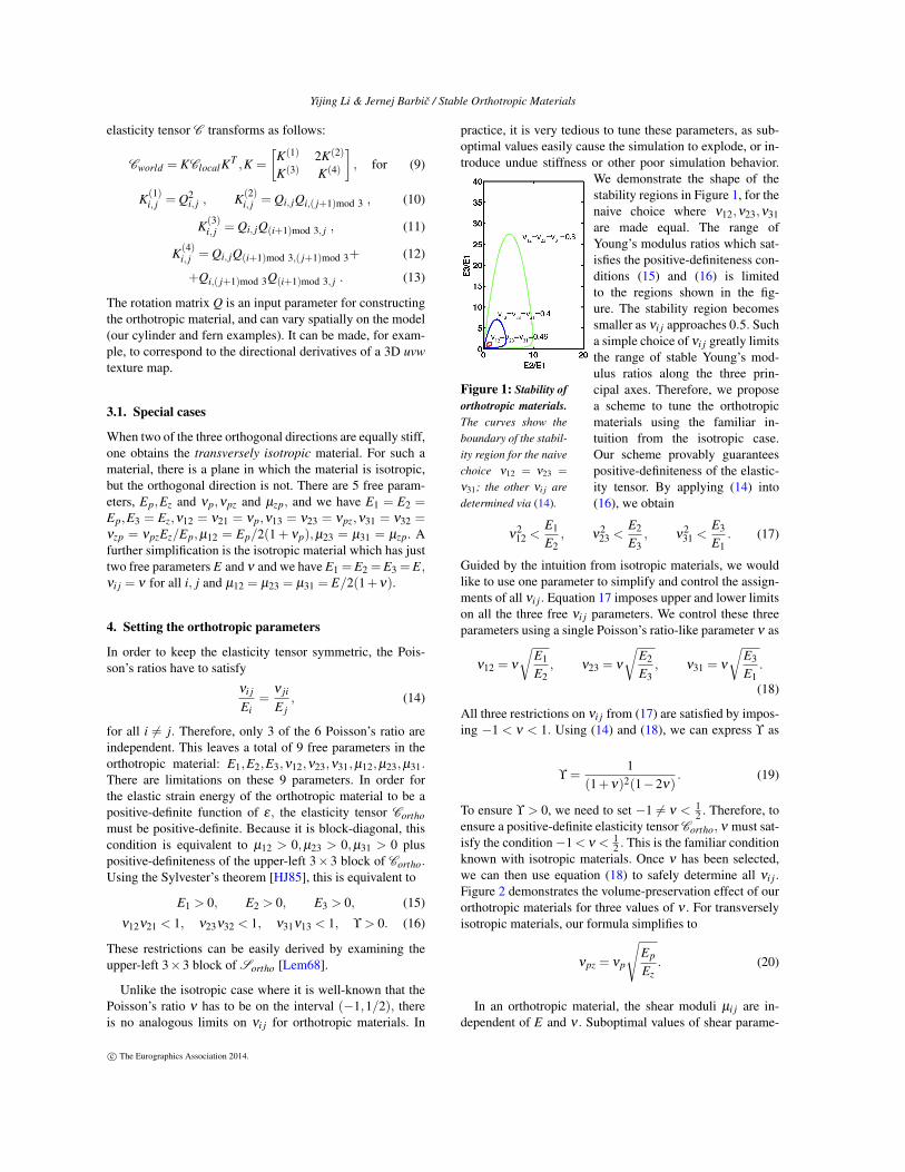
Figure 1: Stability oforthotropic materials.The curves show theboundary of the stabil-ity region for the naivechoice ν12 = ν23 =

ν31; the other νi j aredetermined via (14).

We demonstrate the shape of thestability regions in Figure 1, for thenaive choice where ν12,ν23,ν31are made equal. The range ofYoung’s modulus ratios which sat-isfies the positive-definiteness con-ditions (15) and (16) is limitedto the regions shown in the fig-ure. The stability region becomessmaller as νi j approaches 0.5. Sucha simple choice of νi j greatly limitsthe range of stable Young’s mod-ulus ratios along the three prin-cipal axes. Therefore, we proposea scheme to tune the orthotropicmaterials using the familiar in-tuition from the isotropic case.Our scheme provably guaranteespositive-definiteness of the elastic-ity tensor. By applying (14) into(16), we obtain

ν212 <

E1

E2, ν

223 <

E2

E3, ν

231 <

E3

E1. (17)

Guided by the intuition from isotropic materials, we wouldlike to use one parameter to simplify and control the assign-ments of all νi j. Equation 17 imposes upper and lower limitson all the three free νi j parameters. We control these threeparameters using a single Poisson’s ratio-like parameter ν as

ν12 = ν

√E1

E2, ν23 = ν

√E2

E3, ν31 = ν

√E3

E1.

(18)

All three restrictions on νi j from (17) are satisfied by impos-ing −1 < ν < 1. Using (14) and (18), we can express ϒ as

ϒ =1

(1+ν)2(1−2ν). (19)

To ensure ϒ > 0, we need to set −1 6= ν < 12 . Therefore, to

ensure a positive-definite elasticity tensor Cortho, ν must sat-isfy the condition−1 < ν < 1

2 . This is the familiar conditionknown with isotropic materials. Once ν has been selected,we can then use equation (18) to safely determine all νi j.Figure 2 demonstrates the volume-preservation effect of ourorthotropic materials for three values of ν . For transverselyisotropic materials, our formula simplifies to

νpz = νp

√Ep

Ez. (20)

In an orthotropic material, the shear moduli µi j are in-dependent of E and ν . Suboptimal values of shear parame-

c© The Eurographics Association 2014.

Yijing Li & Jernej Barbic / Stable Orthotropic Materials

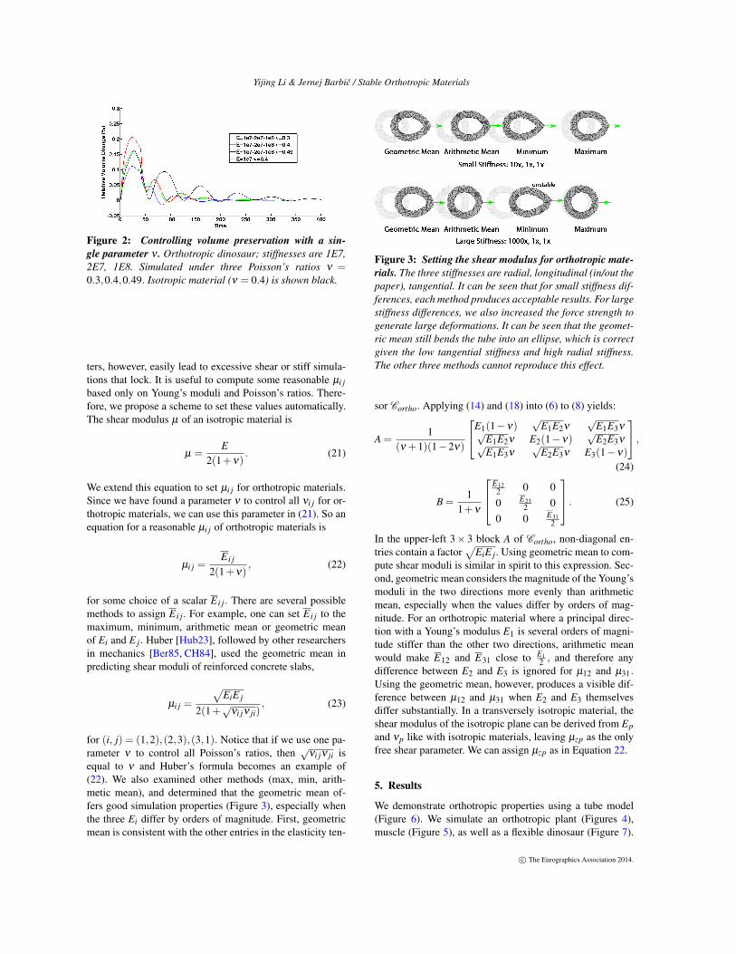
Figure 2: Controlling volume preservation with a sin-gle parameter ν . Orthotropic dinosaur; stiffnesses are 1E7,2E7, 1E8. Simulated under three Poisson’s ratios ν =0.3,0.4,0.49. Isotropic material (ν = 0.4) is shown black.

ters, however, easily lead to excessive shear or stiff simula-tions that lock. It is useful to compute some reasonable µi jbased only on Young’s moduli and Poisson’s ratios. There-fore, we propose a scheme to set these values automatically.The shear modulus µ of an isotropic material is

µ =E

2(1+ν). (21)

We extend this equation to set µi j for orthotropic materials.Since we have found a parameter ν to control all νi j for or-thotropic materials, we can use this parameter in (21). So anequation for a reasonable µi j of orthotropic materials is

µi j =E i j

2(1+ν), (22)

for some choice of a scalar E i j. There are several possiblemethods to assign E i j. For example, one can set E i j to themaximum, minimum, arithmetic mean or geometric meanof Ei and E j. Huber [Hub23], followed by other researchersin mechanics [Ber85, CH84], used the geometric mean inpredicting shear moduli of reinforced concrete slabs,

µi j =

√EiE j

2(1+√νi jν ji), (23)

for (i, j) = (1,2),(2,3),(3,1). Notice that if we use one pa-rameter ν to control all Poisson’s ratios, then √νi jν ji isequal to ν and Huber’s formula becomes an example of(22). We also examined other methods (max, min, arith-metic mean), and determined that the geometric mean of-fers good simulation properties (Figure 3), especially whenthe three Ei differ by orders of magnitude. First, geometricmean is consistent with the other entries in the elasticity ten-

Figure 3: Setting the shear modulus for orthotropic mate-rials. The three stiffnesses are radial, longitudinal (in/out thepaper), tangential. It can be seen that for small stiffness dif-ferences, each method produces acceptable results. For largestiffness differences, we also increased the force strength togenerate large deformations. It can be seen that the geomet-ric mean still bends the tube into an ellipse, which is correctgiven the low tangential stiffness and high radial stiffness.The other three methods cannot reproduce this effect.

sor Cortho. Applying (14) and (18) into (6) to (8) yields:

A =1

(ν +1)(1−2ν)

E1(1−ν)√

E1E2ν√

E1E3ν√E1E2ν E2(1−ν)

√E2E3ν√

E1E3ν√

E2E3ν E3(1−ν)

,(24)

B =1

1+ν

E122 0 00 E23

2 00 0 E31

2

. (25)

In the upper-left 3× 3 block A of Cortho, non-diagonal en-tries contain a factor

√EiE j. Using geometric mean to com-

pute shear moduli is similar in spirit to this expression. Sec-ond, geometric mean considers the magnitude of the Young’smoduli in the two directions more evenly than arithmeticmean, especially when the values differ by orders of mag-nitude. For an orthotropic material where a principal direc-tion with a Young’s modulus E1 is several orders of magni-tude stiffer than the other two directions, arithmetic meanwould make E12 and E31 close to E1

2 , and therefore anydifference between E2 and E3 is ignored for µ12 and µ31.Using the geometric mean, however, produces a visible dif-ference between µ12 and µ31 when E2 and E3 themselvesdiffer substantially. In a transversely isotropic material, theshear modulus of the isotropic plane can be derived from Epand νp like with isotropic materials, leaving µzp as the onlyfree shear parameter. We can assign µzp as in Equation 22.

5. Results

We demonstrate orthotropic properties using a tube model(Figure 6). We simulate an orthotropic plant (Figures 4),muscle (Figure 5), as well as a flexible dinosaur (Figure 7).

c© The Eurographics Association 2014.

Yijing Li & Jernej Barbic / Stable Orthotropic Materials

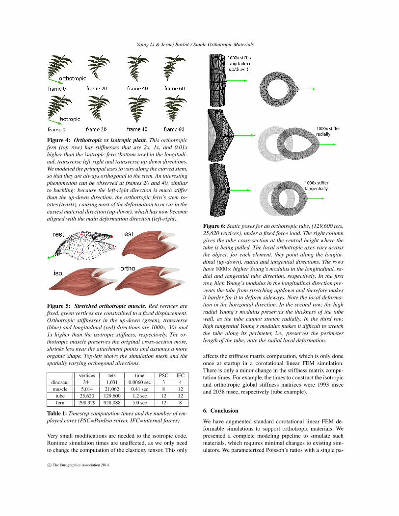
Figure 4: Orthotropic vs isotropic plant. This orthotropicfern (top row) has stiffnesses that are 2x, 1x, and 0.01xhigher than the isotropic fern (bottom row) in the longitudi-nal, transverse left-right and transverse up-down directions.We modeled the principal axes to vary along the curved stem,so that they are always orthogonal to the stem. An interestingphenomenon can be observed at frames 20 and 40, similarto buckling: because the left-right direction is much stifferthan the up-down direction, the orthotropic fern’s stem ro-tates (twists), causing most of the deformation to occur in theeasiest material direction (up-down), which has now becomealigned with the main deformation direction (left-right).

Figure 5: Stretched orthotropic muscle. Red vertices arefixed, green vertices are constrained to a fixed displacement.Orthotropic stiffnesses in the up-down (green), transverse(blue) and longitudinal (red) directions are 1000x, 30x and1x higher than the isotropic stiffness, respectively. The or-thotropic muscle preserves the original cross-section more,shrinks less near the attachment points and assumes a moreorganic shape. Top-left shows the simulation mesh and thespatially varying orthogonal directions.

vertices tets time PSC IFCdinosaur 344 1,031 0.0060 sec 3 4muscle 5,014 21,062 0.41 sec 8 12

tube 25,620 129,600 1.2 sec 12 12fern 298,929 928,088 5.0 sec 12 8

Table 1: Timestep computation times and the number of em-ployed cores (PSC=Pardiso solver, IFC=internal forces).

Very small modifications are needed to the isotropic code.Runtime simulation times are unaffected, as we only needto change the computation of the elasticity tensor. This only

Figure 6: Static poses for an orthotropic tube, (129,600 tets,25,620 vertices), under a fixed force load. The right columngives the tube cross-section at the central height where thetube is being pulled. The local orthotropic axes vary acrossthe object: for each element, they point along the longitu-dinal (up-down), radial and tangential directions. The rowshave 1000× higher Young’s modulus in the longitudinal, ra-dial and tangential tube direction, respectively. In the firstrow, high Young’s modulus in the longitudinal direction pre-vents the tube from stretching up/down and therefore makesit harder for it to deform sideways. Note the local deforma-tion in the horizontal direction. In the second row, the highradial Young’s modulus preserves the thickness of the tubewall, as the tube cannot stretch radially. In the third row,high tangential Young’s modulus makes it difficult to stretchthe tube along its perimeter, i.e., preserves the perimeterlength of the tube; note the radial local deformation.

affects the stiffness matrix computation, which is only doneonce at startup in a corotational linear FEM simulation.There is only a minor change in the stiffness matrix compu-tation times. For example, the times to construct the isotropicand orthotropic global stiffness matrices were 1993 msecand 2038 msec, respectively (tube example).

6. Conclusion

We have augmented standard corotational linear FEM de-formable simulations to support orthotropic materials. Wepresented a complete modeling pipeline to simulate suchmaterials, which requires minimal changes to existing sim-ulators. We parameterized Poisson’s ratios with a single pa-

c© The Eurographics Association 2014.

Yijing Li & Jernej Barbic / Stable Orthotropic Materials

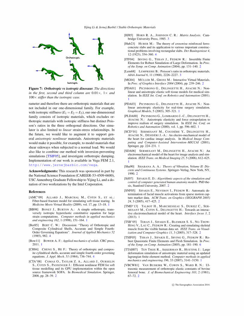
Figure 7: Orthotropic vs isotropic dinosaur. The directionsin the first, second and third column are 0.01×, 1× and100× stiffer than the isotropic case.

rameter and therefore there are orthotropic materials that arenot included in our one-dimensional family. For example,with isotropic stiffness (E1 =E2 =E3), our one-dimensionalfamily consists of isotropic materials, which excludes or-thotropic materials with isotropic stiffness but distinct Pois-son’s ratios in the three orthogonal directions. Our simu-lator is also limited to linear strain-stress relationships. Inthe future, we would like to augment it to support gen-eral anisotropic nonlinear materials. Anisotropic materialswould make it possible, for example, to model materials thatshear sideways when subjected to a normal load. We wouldalso like to combine our method with inversion-preventingsimulations [TSIF05], and investigate orthotropic damping.Implementation of our work is available in Vega FEM 2.1,http://www.jernejbarbic.com/vega.

Acknowledgments: This research was sponsored in part bythe National Science Foundation (CAREER-53-4509-6600),USC Annenberg Graduate Fellowship to Yijing Li, and a do-nation of two workstations by the Intel Corporation.

References[AMC∗09] ALLARD J., MARCHAL M., COTIN S., ET AL.:

Fiber-based fracture model for simulating soft tissue tearing. InMedicine Meets Virtual Reality (2009), vol. 17, pp. 13–18. 1

[BB98] BONET J., BURTON A.: A simple orthotropic, trans-versely isotropic hyperelastic constitutive equation for largestrain computations. Computer methods in applied mechanicsand engineering 162, 1 (1998), 151–164. 1

[Ber85] BERT C. W.: Discussion: “Theory of Orthotropic andComposite Cylindrical Shells, Accurate and Simple Fourth-Order Governing Equations”. Journal of Applied Mechanics 52(1985), 982. 4

[Bow11] BOWER A. F.: Applied mechanics of solids. CRC press,2011. 1

[CH84] CHENG S., HE F.: Theory of orthotropic and compos-ite cylindrical shells, accurate and simple fourth-order governingequations. J. Appl. Mech. 51 (1984), 736–744. 4

[CTA∗08] COMAS O., TAYLOR Z. A., ALLARD J., OURSELINS., COTIN S., PASSENGER J.: Efficient nonlinear FEM for softtissue modelling and its GPU implementation within the opensource framework SOFA. In Biomedical Simulation. Springer,2008, pp. 28–39. 2

[HJ85] HORN R. A., JOHNSON C. R.: Matrix Analysis. Cam-bridge University Press, 1985. 3

[Hub23] HUBER M.: The theory of crosswise reinforced ferro-concrete slabs and its application to various important construc-tional problems involving rectangular slabs. Der Bauingenieur 4,12 (1923), 354–360. 4

[ITF04] IRVING G., TERAN J., FEDKIW R.: Invertible FiniteElements for Robust Simulation of Large Deformation. In Proc.of the Symp. on Comp. Animation (2004), pp. 131–140. 2

[Lem68] LEMPRIERE B.: Poisson’s ratio in orthotropic materials.AIAA Journal 6, 11 (1968), 2226–2227. 3

[MG04] MÜLLER M., GROSS M.: Interactive Virtual Materials.In Proc. of Graphics Interface 2004 (2004), pp. 239–246. 2

[PDA01] PICINBONO G., DELINGETTE H., AYACHE N.: Non-linear and anisotropic elastic soft tissue models for medical sim-ulation. In IEEE Int. Conf. on Robotics and Automation (2001).1

[PDA03] PICINBONO G., DELINGETTE H., AYACHE N.: Non-linear anisotropic elasticity for real-time surgery simulation.Graphical Models, 5 (2003), 305–321. 1

[PLDA00] PICINBONO G., LOMBARDO J.-C., DELINGETTE H.,AYACHE N.: Anisotropic elasticity and force extrapolation toimprove realism of surgery simulation. In IEEE Int. Conf. onRobotics and Automation (2000), vol. 1, pp. 596–602. 1

[SCD∗01] SERMESANT M., COUDIÈRE Y., DELINGETTE H.,AYACHE N., DÉSIDÉRI J.-A.: An electro-mechanical model ofthe heart for cardiac image analysis. In Medical Image Com-puting and Computer-Assisted Intervention–MICCAI (2001),Springer, pp. 224–231. 1

[SDA06] SERMESANT M., DELINGETTE H., AYACHE N.: Anelectromechanical model of the heart for image analysis and sim-ulation. IEEE Trans. on Medical Imaging 25, 5 (2006), 612–625.1

[Sha90] SHABANA A. A.: Theory of Vibration, Volume II: Dis-crete and Continuous Systems. Springer–Verlag, New York, NY,1990. 2

[Sif07] SIFAKIS E. D.: Algorithmic aspects of the simulation andcontrol of computer generated human anatomy models. PhD the-sis, Stanford University, 2007. 2

[SNF05] SIFAKIS E., NEVEROV I., FEDKIW R.: Automatic de-termination of facial muscle activations from sparse motion cap-ture marker data. ACM Trans. on Graphics (SIGGRAPH 2005)24, 3 (2005), 417–425. 2

[TMD∗13] TALBOT H., MARCHESSEAU S., DURIEZ C., SER-MESANT M., COTIN S., DELINGETTE H.: Towards an interac-tive electromechanical model of the heart. Interface focus 3, 2(2013). 1

[TSB∗05] TERAN J., SIFAKIS E., BLEMKER S. S., NG-THOW-HING V., LAU C., FEDKIW R.: Creating and simulating skeletalmuscle from the visible human data set. IEEE Trans. on Visual-ization and Computer Graphics 11, 3 (2005), 317–328. 2

[TSIF05] TERAN J., SIFAKIS E., IRVING G., FEDKIW R.: Ro-bust Quasistatic Finite Elements and Flesh Simulation. In Proc.of the Symp. on Comp. Animation (2005), pp. 181–190. 6

[TTAH07] TEN THIJE R., AKKERMAN R., HUETINK J.: Largedeformation simulation of anisotropic material using an updatedlagrangian finite element method. Computer methods in appliedmechanics and engineering 196, 33 (2007), 3141–3150. 1

[VBCW81] VAN BUSKIRK W., COWIN S., WARD R. N.: Ul-trasonic measurement of orthotropic elastic constants of bovinefemoral bone. J. of Biomechanical Engineering 103, 2 (1981),67–72. 2

c© The Eurographics Association 2014.