Embed Size (px)
Citation preview

1
Microscopie confocale
Start Pane

2
Introduction & Généralités
Principe de la microscopie confocale
Fluorescence – Sondes Fluorescentes et intérêts en biologie
Confocalité – avantages
Setup expérimental
Paramétrage d‘images
Applications
3D / Reconstruction d‘images
Quantifications
Macros
Deconvolution (PSF)
Limitations
Etudes de colocalisation
Calibration
Résolution

3
Généralités
Introduction
Principe de la microscopie confocale
Fluorescence – Sondes Fluorescentes et intérêts en biologie
Confocalité – avantages
Setup expérimental
Paramétrage d‘images
Applications
3D / Reconstruction d‘images
Quantifications
Macros
Deconvolution (PSF)
Limitations
Etudes de colocalisation
Calibration
Résolution

4
Introduction
Historique
La microscopie photonique a été inventée au XVIIe siècle mais c'est à partir
du XIXe siècle qu'elle devient un outil indispensable pour les grandes
découvertes en biologie. La cellule découverte par Hooke en 1665 à l'aide d'un
microscope rudimentaire est précisée par Purkinje en 1825. La découverte du
noyau est faite par Brown en 1831. On découvre alors la division cellulaire et le
rôle du noyau. La microscopie photonique permet la découverte d'agents
pathogènes : le bacille de la lèpre par Hansen en 1874, de la tuberculose par
Koch en 1882, de la peste par Yersin en 1894.
Parallèlement à ces découvertes, les techniques de microscopie progressent. Le
premier microscope inversé date de 1850, et le premier condenseur permettant
d'optimiser l'éclairage est mis au point par Abbe en 1872, et optimisé par Köhler
en 1893.
La microscopie de fluorescence est imaginée par Reichert en 1908, puis
expérimentée avec des fluorochromes par Haitinger en 1911. Le contraste de
phase, décrit par Zernike date de 1934, et le contraste interférentiel est mis au
point par Nomarski en 1952.

5
World of small structures
Introduction

6
Cell Diagram, A small world of high complexity
Introduction

7
Introduction

8
ESSENTIALS
• Magnification : The way to see small detail
• Resolution : The way to distinguish between small detail
• Contrast : The way to see resolved and magnified detail
To see the Micro-cosmos
We need Microscopy
Introduction

9
• Human eye : 100000 nm
• Simple magnifier : 10000 nm
• Optical microscope : 200 nm limits
• Electron microscope : 0.5 – 3 nm
• Scanning Probe microscope : 0.1 – 10 nm
Microscopical range
Introduction

10
Imaging Modes
BF
PH
DIC
FL
Introduction

11
• Only specific structures are stained and images
• Unwanted structures remain are not visible
• Detail can be seen even if smaller than resolution limits
• With the advent of special dyes, staining of living cells is now possible
Contrast using Fluorescence
Introduction

12
Fluorescence
Jablonski Diagram
Energy
Prof. Alexander Jablonski, 1935
Absorption
Emission
Stokes-Shift
488nm
525nm
E = hn = hc/l
Excited Energy levels
Ground Energy levels

13
Prof. Alexander Jablonski, 1935
E = hn = hc/l
Principe - Fluorescence

14
Principe - Fluorescence

15
Dichroic spectral position
Principe - Fluorescence

16
Ultraviolets InfrarougesVisible
400 nm 700 nm
Sources lumineuses
Principe - Fluorescence

17
Principe - Fluorescence

18
Principe - Fluorescence

19
Prof. Ploem’s invention
Principe - Fluorescence

20
Principe - Fluorescence

21
Principe - Fluorescence
Sondes fluorescentes et intérêts en biologie

22
• sans modulation
dichroïque
• jusqu‘au 200 points
chaque spectre
• 2-5 nm résolution
xFP Spectra
0
0.2
0.4
0.6
0.8
1
400 450 500 550 600 650 700
wavelength (nm)
No
rmalized
CFP
BFP
eGFP
YFP
dsRed
Leica TCS SP2 AOBS: vrais spectres
In-situ Fluorescence protein spectraCourtesy Dr. T. Zimermann, EMBL, Heidelberg, Germany
23
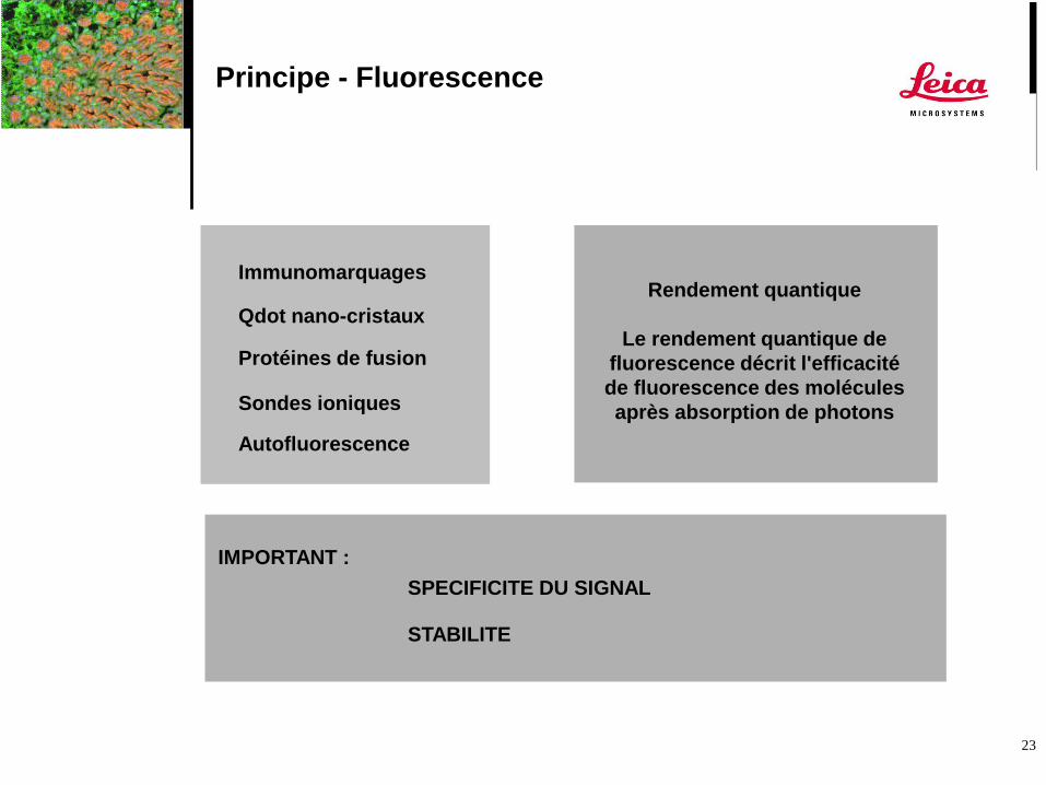
Principe - Fluorescence
Immunomarquages
Protéines de fusion
Autofluorescence
Sondes ioniques
Qdot nano-cristaux
Rendement quantique
Le rendement quantique de
fluorescence décrit l'efficacité
de fluorescence des molécules
après absorption de photons
SPECIFICITE DU SIGNAL
IMPORTANT :
STABILITE

24
Red Fluorescent Proteins

25
Red Fluorescent Proteins
Ref.: Campbell et al.
2002, PNAS, Vol. 99,
no.12: 7877-82
•DsRed
•mRFP1

26
Laser Orange 594 nm:
Nouveaux Fluorochrome, Excitation Optimal
Fluorochrome excité par 594 nm Excitation [nm] Emission [nm]
Alexa 568 577 603
5-ROX 578 604
HC Red 590 614
SNARF (carboxy) pH 9 576 639
Alexa 594 594 618
Bodipy TR-X SE 588 616
Calcium Crimson 588 611
CTC 5-cyano-2,3-ditolyl-Tetrazolium-Chloride 602 630
Red FluoSpheres 580 603
Texas Red 595 620
YO-PRO-3 613 629

27
Généralités
Introduction
Principe de la microscopie confocale
Fluorescence – Sondes Fluorescentes et intérêts en biologie
Confocalité – avantages
Multiphoton
Setup expérimental
Paramétrage d‘images
Applications
3D / Reconstruction d‘images
Quantifications
Macros
Deconvolution (PSF)
Limitations
Etudes de colocalisation
Calibration
Résolution

28
Microscopie confocale
Conventional vs Confocal

29
Résolution optimale Intensité de fluorescence
maximale
Microscopie confocale

30
Basement membrane labeled with cy2 (green)Neurons labeled with cy3 (red)
Résolution

31
Confocal Microscopy
• Patented by Minsky in 1957
• Elimination the out of focus flare observed influorescence in thick sections

32
Confocal Microscopy Benefits
Suppression of out of focus light
The confocal detection pinhole acts as a barrier
To light outside the focal plane of the objective
Optical sectioning:
Specimen is monitored slice by slice (3D-resolution)
Each slice produces a sharp image by confocal optics
Improved resolution power:
Lateral resolution improved by appr. 1.4x.
Significant improvement in axial resolution
Improved contrast:
Rasterizing the specimen, straylight due to scattering is suppressed
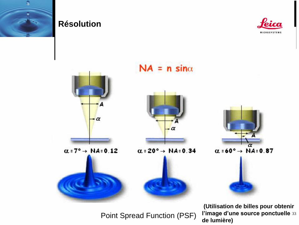
33Point Spread Function (PSF)
Résolution
(Utilisation de billes pour obtenir
l’image d’une source ponctuelle
de lumière)

35
XY Plane
Airy disc
Limited by Diffraction
D0 = 1.22 * l / NA (lateral)
XZ Plane
Résolution

36
Airy Disk formation
Airy Disk Formation

37
Fluorescence Resolution
Res = 0.61*l / NA
credit: http://www.microscopyu.com/tutorials/

38
Imaging of small fluoresence beads
Vignette credit: http://www.microscopyu.com/tutorials/

39
Vignette credit: http://www.microscopyu.com/tutorials/
Imaging of small fluoresence beads

40
Vignette credit: http://www.microscopyu.com/tutorials/
Imaging of small fluoresence beads

41
Resolution Widefiled vs Confocal
Credit : Prof. A. Diaspro
Conventional Confocal

42
Généralités
Introduction
Principe de la microscopie confocale
Fluorescence – Sondes Fluorescentes et intérêts en biologie
Confocalité – avantages
Setup expérimental
Paramétrage d‘images
Applications
3D / Reconstruction d‘images
Quantifications
Macros
Deconvolution (PSF)
Limitations
Etudes de colocalisation
Calibration
Résolution

43
Confocal Implementation
Requires to excite and observe as small a
volume as possible on the sample.
This in turn requires a different way of
illumination and observation of the samples

Laser types

45
Confocal Beam Path

46
Confocal Principle

47
Scanning the Sample

48
Why Laser ?
• Intense light source confined to small beam size
Easily focused to diffraction limited spot
• Coherence is not required (can cause problems)
• As different fluorescence dyes have different
spectral characteristics, many laser lines are
required

49
Why scanning?
• Scanning in xy is necessary in order to form an image
• The scanning device is positioned between the beam
splitter and the objective
• The beam is scanned (made to move) on the excitation
side and descanned (made stationary) on the detection
side

50
Why a standard microscope ?
• Greatly facilitates the use of the system
• Provides a platform for mounting samples
• The application determines what type of microscope to be used

51
Microscope types
Inverted :
Live specimens
Upright : fixed samples
Fixed stage :
Patch clamping

52
Microscopie confocale

53
Microscopie confocale

54
AOTF (Acousto Optical Tunable Filter)
Module de sélection d’excitation
Source de lumière:
Laser multilinie ou
plusieurs lasers
couplés par fibre
• Libre sélection de ligne
• Contrôle indépendent de l‘intensité
sur chaque lineAOTF

55
Acousto Optical Beam Splitter:
Dichroïc Électronique

56
• Selectivité parfaite
•Transparence
le plus haut possible
• Plus “d’espace” pour
détecter les emissions
AOBS transmission

57
Microscopie confocale

58
SP Detector - Advantages
• N'importe quelle spécification de filtre est
librement programmable
• Caractéristiques très étroite permet la
détection de plus de fluorescence
• Aucun élément filtre dans le trajet – plus de
transmission
• Balayage spectral avec haute résolution
(2-5nm, 200 steps)

59
Sectionnement optique de l‘échantillon
Suppression de la fluorescence en dehors du plan focal
Amélioration de la résolution latérale et axiale
Amélioration du contraste
Microscopie confocale

The Digital Image
How is the optical image relayed on to a
screen
A digital image ?
61
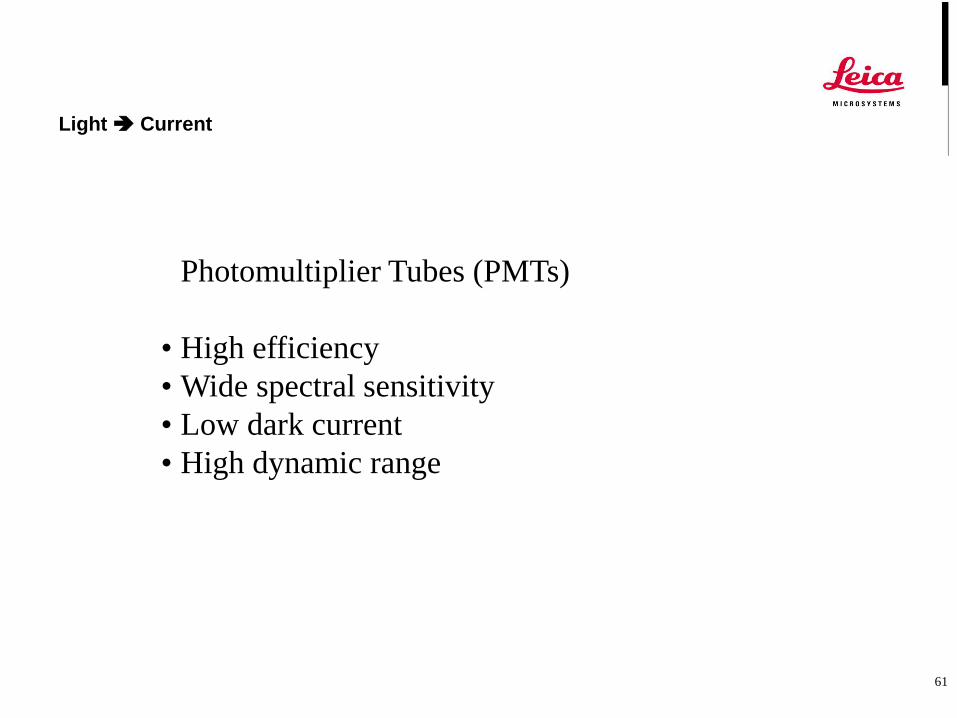
Light Current
Photomultiplier Tubes (PMTs)
• High efficiency
• Wide spectral sensitivity
• Low dark current
• High dynamic range

62
Ca
tho
de
ra
dia
nt se
nsitiv
ity (
mA
/W)
--
--
Quantu
m e
ffic
iency(%
)
Longueur d’onde (nm)
100 200 600 700 800 900 1000300 400 500
0,1
1
10
100
Setup expérimental
Détection : photomultiplicateurs
Conversion d’une détection de
photons en signal électrique

63
APD
• higher sensitivity
• low background
• smaller dynamic range
• only a certain amount
of photons/time allowed
PMT
• lower sensitivity
• higher background
• bigger dynamic range
weak
samplesbright
samples
Setup expérimental

64
Current Digits (Digitazitation)
ADC Converter8bit / 12 bit (= 256 / 4096 Greyvalues)
Frame Store
Data Files (e.g. TIF)
About Data:
8 Sections 512x512 8bit 1ch: 2 MB
100 Sections 4096x4096 12 bit 5ch: 6000 MB

65
Digits Paper
Monitor
Printer
Slidemaker
PPT Präsentation
HTML Document

66

67
Objective Lens
Needs for confocal imaging:
• High aperture
• High colour correction
• Flat field
• Long working distance
• High transmittance
• Variety of coupling media
i.e. Plan Apochromat &
Plan-Fluotar

68
Objectif Glycérol :
Comparaison: Objectif à huile vs. Glycérol
yz
xz
Objectif Glycérol PL APO 63x1.3 Objectif huile PL APO 63x1.32
center section center section
Sample: muscle fibers embedded in Glycerol (80/20%) thickness ca. 100µm

69
Courbes de transmission des objectifs

70
Généralités
Introduction
Principe de la microscopie confocale
Fluorescence – Sondes Fluorescentes et intérêts en biologie
Confocalité – avantages
Setup expérimental
Paramétrage d‘images
Applications
3D / Reconstruction d‘images
Quantifications
Macros
Deconvolution (PSF)
Limitations
Etudes de colocalisation
Calibration
Résolution

71
Paramétrage d’image
Mode de scan
Fréquence de balayage laser
Objectif utilisé
Zoom optique appliqué
Format d’image
Rotation de scan
Moyennage d’images
Accumulation
Gain du PMT
Offset du PMT
…

72
Immunohistochimie
© INRA Versailles IJPB LCC© INRA Versailles IJPB LCC

73
Généralités
Introduction
Principe de la microscopie confocale
Fluorescence – Sondes Fluorescentes et intérêts en biologie
Confocalité – avantages
Setup expérimental
Paramétrage d‘images
Applications
3D / Reconstruction d‘images
Quantifications
Macros
Deconvolution (PSF)
Limitations
Etudes de colocalisation
Calibration
Résolution

74© INRA Versailles IJPB LCC
Immunohistochimie

75© INRA Versailles IJPB LCC
Immunohistochimie

76© INRA Versailles IJPB LCC
Immunohistochimie

77
l exc = 405 nm
l ém. = 422-496
l exc = 488 nm
l ém. = 496-533
l exc = 543 nm
l ém. = 556-628 nm
l exc = 633 nm
l ém. = 661-690 nm
T. Lecuit, Luminy, Marseille
Obj. 40X, 1.25
Zoom = 4,7
Embryon Drosophile
Immunohistochimie

78
Immunohistochimie

79
Immunohistochimie

80
Réflection
Etude de surface

81
Réflection

82
Time-Lapse
Arabidopsis thaliana
First channel: Cell wall in reflection.
2 & 3 channel: Monitoring mitochondrial (GFP-green) and plastid
(autofluorescence-red) movement.
22 fps
Courtesy of Prof. Dr. D. Menzel, Institut für Zelluläre und Molekulare Botanik
Zellbiologie der Pflanzen, Bonn University.

83
Fluorescence Recovery After Photobleaching

84
Région Bleachée
Région
adjacente
à la région
BleachéeI= f(t)
T. Lecuit, Luminy, Marseillelexc. = 488 nm
Obj. 63X, 1.32
Zoom = 4,6
Dt = 823 ms
Fluorescence Recovery After Photobleaching

85
Fluorescence Resonance Energy Transfer

86
Fluorescence Resonance Energy Transfer
Etude des modifications des
interactions moléculaires
Proximité donneur-accepteur 10–100 Å
Donor pre-bleach
Donor post-bleach
Acceptor pre-bleach
Acceptor post-bleach
Bleaching de l’accepteur
Augmentation de l’intensité de
fluorescence du donneur

87
Application FRET-AB
Setup pour imager
le donneur et l‘accepteur
Donneur
Accepteur
SP5 – LAS AF

88
Application FRET-AB
Setup du bleach
pour l‘accepteur
SP5 – LAS AF

89
Application FRET-AB
Quantification
Step 3
FRET-Efficiency
SP5 – LAS AF
90
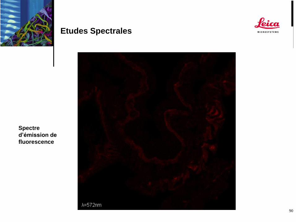
Etudes Spectrales
Spectre
d’émission de
fluorescence

91
Etudes Spectrales
Spectres d’émission de fluorescence

92
Alexa 488 – GFP
Etudes Spectrales
Séparation spectrale

93
Example
FITC/TxR sample
2 channel recording:•Detection bands fine tuned
•No gaps between bands
•High efficient prism
•High efficient PMTs
•AOBS® applied

94
FITC
The total of all light collected from
FITC molecules will be distributed
into both channels.
We assume here:
¾ of all FITC emission go into the
green channel (G)
¼ of all FITC emission goes into the
red channel (R)

95
TxR
The total of all light collected from
TxR molecules will be distributed
into both channels.
We assume here:
1/5 of all TxR emission goes into the
green channel (G)
4/5 of all FITC emission goes into
the red channel (R)
96
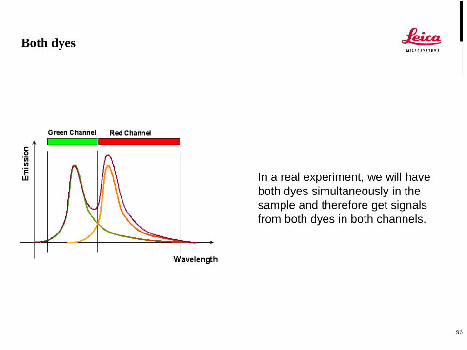
Both dyes
In a real experiment, we will have
both dyes simultaneously in the
sample and therefore get signals
from both dyes in both channels.

97
A calculated measurement
TxR5
4FITC
4
1R
TxR5
1FITC
4
3G
98
Spectra: # and d
Important Note:
Theoretical spectrum: infinite number of datapoints.
Reality: maybe 50 channels, or just 2
Equidistant measurement is a good thing. But it is not always necessary.
In the unmix case, equidistance is no good: better to tune the bandwidth and
center wavelength. So we optimize S/N for separating data later.
Requires important hardware features as tunable bands, any filter
characteristic etc. which you find only with the Leica SP design.

99
What we dont‘t need:
Important note: it is sufficient to have two equations for
2 unknowns.
Those systems providing more and equidistant
channels (with gaps in between) are technically
massively inferior to the Leica SP AOBS concept.
TxR5
4FITC
4
1R
TxR5
1FITC
4
3G
This is just a set of n linear equations with n unkowns.
You may remember from primary school.
3y+2x=7
7y+ x=2
There are methods, to solve these by computers

100
Contributions
Unmixing is:
Solving sets of n linear
equations with n unknowns.
First proven records of
solutions go back some 4000
years (Egypt)
For a reference see:http://www.ETH\EducETH - Mathematik -
Leitprogramm Lineare
Gleichungssysteme.htm

101
Math Solution
1. Guess coefficients and subtract manually bleed through
Manual Dye Separation
2. Take n channel image, have pure dyes somewhere and let the
computer solve
Channel Dye Separation
3. Take a spectrum, have the spectra from the pure dyes and let the
computer solve
Spectral Dye Separation

102
Stat Solution
Let computer find best fitting line for clouds. Angle corresponds to
coefficients.
Adaptive Dye Separation
1. Let computer bend lines to coincide with axes
strong
2. Let computer bend until first non-empty bin hits the axis
weak
3. Find projection of n dimensions, when n dyes around
Dimensionality reduction (this is not an unmixing method)

103
Emission control:
SP performance test
Alexa 488 – GFP:
Almost complete
spectral overlap700650600
wavelength (nm)
550500450400
0
0,2
0,4
0,6
1
0,8
1,2
Alexa
GFP

104
1s 10s 12s 17s
32s 42s 52s 62s
GFP Photoactivable
Pulse laser IR 60 ms 800 nm
D. Choquet, Institut François Magendie, UMR 5091 CNRS, Bordeaux.Physiologie cellulaire de la synapse

105
Fluorescence Correlation Spectroscopy
Lien entre la diffusion de molécules et la fluctuation de l’intensité de
fluorescence dans un volume donné
Concentration
Coefficient de diffusion
Constante de dissociation

106
Fluorescence Correlation Spectroscopy

107
Généralités
Introduction
Principe de la microscopie confocale
Fluorescence – Sondes Fluorescentes et intérêts en biologie
Confocalité – avantages
Setup expérimental
Paramétrage d‘images
Applications
3D / Reconstruction d‘images
Quantifications
Macros
Deconvolution (PSF)
Limitations
Etudes de colocalisation
Calibration
Résolution

108
Etude de colocalisation
Immunohistochimie
109
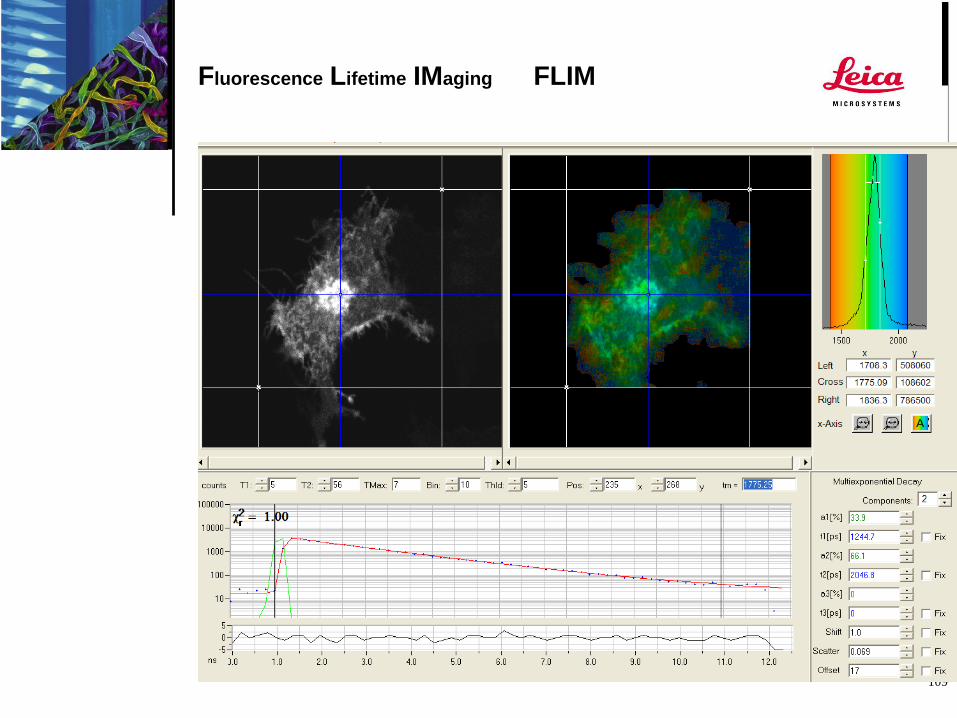
Fluorescence Lifetime IMaging FLIM

110
Fluorescence Lifetime IMaging FLIM

111
Probe: lexc/lem a (ns) b (ns)
BCECF 490/520 3.0 (acid) 3.8 (base)
Fluo-3
Lucifer Yellow
Sodium Green
Hoechst
490/520 2.44 (no Ca2+)
3.3
1.1 (low Na+)
2.2 (no acc., 7-AAD)
0.79 (Ca2+)
2.4 (high Na+)
1.4 (acceptor,7-AAD)
FITC
TRITC
490/520
543/
4.0 (pH > 7)
2.0
3.0 (pH < 3)
Rhodamine 700
Rhodamine 700
Cy3
Cy5
659/669
550/570
633/
1.6 (pH 9)
1.55 (H2O)
0.27
1.0
1.55 (pH 6)
2.99 (Ethanol)
0.5 (antibody conjug.)
GFP free (S65T)
CFP
YFP
488/507 2.68
1.3
3.7
Fluorophores and lifetimes

112
Fluorescence lifetime
fluo
rescenceex
cita
tio
n
S0
S1
add
ition
al pro
cesses
red
exponential decay e–t/
time after excitation
flu
ore
scen
ce s
ign
al
fluorescence lifetime:
• ave. time betw. excitation and emission
• characteristic property of dyes, ~ns
• depends on environment (ions, pH, …)

113
Fluorescence lifetime imaging (FLIM)
• measurement of lifetime with spatial resolution
• transformation of nanoseconds in color code

114
Leica TCS SP2 and D-FLIM
CFP-MHC
Cyan: CFP tagged to MHC(Major Histocompatibility Complex)
Before (A) and after (B) FLIM acquisition
1.25 3.5
Courtesy
Dan Davis, Imperial College London
A
B
Duration for acquisition: 200 s
405 nm 405 nm

115
Leica D-FLIM: CFP-MHC
A: Lifetime image
B: Lifetime distribu-
tion over the image
area
C: Fitted decay curve
(corresponding to the pixels selected by the blue cursor in A)
A
C
B
CFP tagged to MHC

116
Leica TCS SP2 and D-FLIM
FluoCells (BPAE)
Blue: 1.5 - 2.2 ns
Red: 2.2 - 2.6 ns
Green: 2.6 - 4.0 ns
Blue: DAPI (nucleus)
Red: Mitotracker Red (mitochondria)
Green: BODIPY FL phallacidin (actin)
405+488+543 nm 405 nm
Molecular Probes, F-14780

117
Leica D-FLIM: FluoCells
A B
C
A: Intensity image
B: Lifetime image
C: Fitted decay curve
(corresponding to the pixels selected by the blue cursor in A)
Blue: DAPI (nucleus)
Red: Mitotracker Red
(mitochondria)
Green: BODIPY FL
phallacidin (actin fibres)

118
Principe de l’excitation à deux photons
Processus de fluorescence en
excitation à deux photons
Deux photons d’énergie deux fois plus
faible (et donc de longueur d’onde deux
fois plus élevée) sont absorbés par la
molécule dans un laps de 10-16 s
hvex
2
S
1
S
0
hvem
Processus de fluorescence en
excitation à un photon
S
1
hvex hvem
S
0
E = hc/l
L’énergie d’un seul photon est absorbée
par un fluorochrome pour passer d’un
état d’énergie basal (S0) à un état excité
(S1)
Les caractéristiques du rayonnement émis par le fluorochrome en
excitation à deux photons sont inchangées
hvex
2
Perte d’énergie
vibrationnelle
Fluorescence

119
Plan
focal
En microscopie à balayage laser à deux photons, l’excitation est
strictement restreinte au volume focal
Fluorescence suite à une
absorption à un photon
Fluorescence suite à une
absorption à deux photons

120
Leica TCS STED

121
Multicolor Image of the NMJ
Liprin-a
STEDBruchpilot
confocal
1 µm500 nm
Courtesy of Prof. Stephan Sigrist

122
Resolution Increase by STED: Pure Physics!
confocalSTEDSTED +
deconvolution
STED is pure physics! But you can add mathematics on top!

123
Optical pathway
Confocal Profile
0 200 400 600 800 1000
x / nm
y
x
STED Profile
0 200 400 600 800 1000
x / nm
y
x
Typical lateral resolution: 200x200 nm Typical lateral FWHM in STED is 90x90 nm
Principle of STED microscopy
1. Excitation laser
2. Depletion laser
3. Original Excitation spot
4. Depletion (STED) ring
5. Effective excitation spot
6. Confocal pinhole
7. Detector
Formation of presynaptic
active zone (Liprin)
Courtesy S. Sigrist,
Wuerzburg

124
ACTIN
Confocal
STED
MICROTUBULES
Confocal
STED

125
The task
Microtubules of a
Vero cell
SOME EXAMPLES:
Neurophysiology (Synapse-cell-interactions, motoneurons etc.)
Endocytotic processes
Virus biology (Malaria, AIDS)
Pathology (Multiple Sclerosis etc.)
Increase xy resolution in fluorescence microscopy over
classical Abbe limits:
a
l
sin2
nd xy FWHMconfocal, xy: 200 nm
BUT: For numerous applications a higher resolution is required
-without the efforts and restrictions of an Electron microscope!-

126
The task
Microtubules of a
Vero cell
SOME EXAMPLES:
Neurophysiology (Synapse-cell-interactions, motoneurons etc.)
Endocytotic processes
Virus biology (Malaria, AIDS)
Pathology (Multiple Sclerosis etc.)
Increase xy resolution in fluorescence microscopy over
classical Abbe limits:
a
l
sin2
nd xy FWHMconfocal, xy: 200 nm
BUT: For numerous applications a higher resolution is required
-without the efforts and restrictions of an Electron microscope!-

127
Applications Example - Cell Biology
F-Actin -Tubulin
STED
Confocal
Nice for demonstrational purposes

128
Resolution enhancement by STED:
confocal
STED STED
STED STED STED
STEDSTEDSTED
STED
Excitation
spot
Depletion
ring
Overlaid
spots
Effective
spot
FWHM
ca. 250nmFWHM
ca. 90nm
A threefold improved resolution can make 9 spots out of 1 !

129
Superresolution Microscopy: Leica TCS 4Pi

130
The target of 4Pi microscopy
Increase axial resolution in fluorescence microscopy over
classical Abbé Limits
Inventor: Stefan Hell, Max Planck Institute for Nanobiophotonics,
Goettingen, Germany
a
l
sin
4.0
nFWHMxy
a
l
cos1
45.0
nFWHMz
xy resolution: ~ 200nm
z resolution (confocal): ~ 500nm

131
The solution: 4Pi microscopy
Confocal focus cross section 4Pi focus cross section
500 nm
4Pi microscopy combines the Numerical Aperture of 2 opposing
objectives through interference
The 4Pi focus volume is a factor 3 – 5 times smaller than the confocal focus
The axial resolution at the excitation wavelength of 780 nm is 110nm
Interference side lobes are removed by linear point deconvolution
x
z

132
Live yeast cell –
mitochondrial
protein distribution
Label: GFP
Objective: 63x1,2 W
Confocal
4Pi
4
m
Jörg Bewersdorf
MPI for Biophysical Chemistry
Göttingen
4Pi microscopy – spectacular 3D resolution
4
m

133
Central element: the 4Pi Interferometer
Illumination and imaging
from both sides, phase-
and wavefront-corrected
Two photon / confocal
system for scanning

134
Leica TCS 4Pi: complete system

135
Parasitology: Human red blood cell - healthy
Cell membrane
(Band-III protein)
labelled with
Qdot®-585 coupled
antibodies
4Pi – 3D rendering
Objective: Glycerol
100x/1,35 CORR
Cell diameter: ca. 8 m
Dr. J.A. Dvorak and Dr. F.Tokumasu,
National Institute of Allergy and Infectious Diseases, NIH, Washington (USA)

136
Parasitology: Human red blood cells -
healthy and Malaria infected - early stage
Band III – protein labelled
with QDot® 585-coupled
antibodies
Plasmodia (yellow, DNA)
stained with Hoechst 33258
4Pi – 3D rendering
Objective: Glycerol
100x/1,35 CORR
Cell diameters: ca. 8 m
Dr. J.A. Dvorak and Dr. F.Tokumasu,
National Institute of Allergy and Infectious Diseases, NIH, Washington (USA)

137
Parasitology: Human red blood cell
Malaria infected – late stage
Band III – protein labelled
with QDot®-585
coupled antibodies
Plasmodia (yellow, DNA)
stained with Hoechst 33258
4Pi – 3D rendering
Objective: Glycerol
100x/1,35 CORR
Cell diameter: ca. 4 m
Dr. J.A. Dvorak and Dr. F.Tokumasu,
National Institute of Allergy and Infectious Diseases, NIH, Washington (USA)

138
Information exchange via the
Plasma Membrane is blocked
in mutated cell
Objective: 63x /1,20 W
Water immersion
Label: GFP
Cell diameter: ca. 8 m
Immunology: MHC-II transport in B-Cells
Jörg Bewersdorf, MPI for Biophysical Chemistry, Göttingen,
You-Mi Kim, Havard Medical, Boston
Healthy cell
4Pi
Mutated cell
4Pi

139
Summary: Leica TCS 4Pi
Nov. 2003 Cover Page3D image of the mitochondrial compartment of a live yeast cell obtained through volume rendering of a superresolution 3D data stack recorded with a 4Pi
microscope. Courtesy of H. Gugel, R. Storz (Leica Microsystems CMS GmbH, Mannheim, Germany) and J. Bewersdorf, S. Jakobs, J. Engelhardt, S.W. Hell
(MPI for Biophysical Chemistry, Göttingen, Germany). The 3D image is superimposed on a colored high resolution scanning electron micrograph of
mitochondria and rough endoplasmic reticulum. © PhotoResearchers. Artwork rendered by Erin Boyle.
Commercial 4Pi microscope
delivers spectacular 3D resolution
Improved sub-cellular imaging
gives visual confirmation of
functional details

140
SuperK - the White Light Laser
Martin Hoppe, Rolf BorlinghausLeica Microsystems CMS GmbH
Am Friedensplatz 3, 68165 MannheimGermany
141
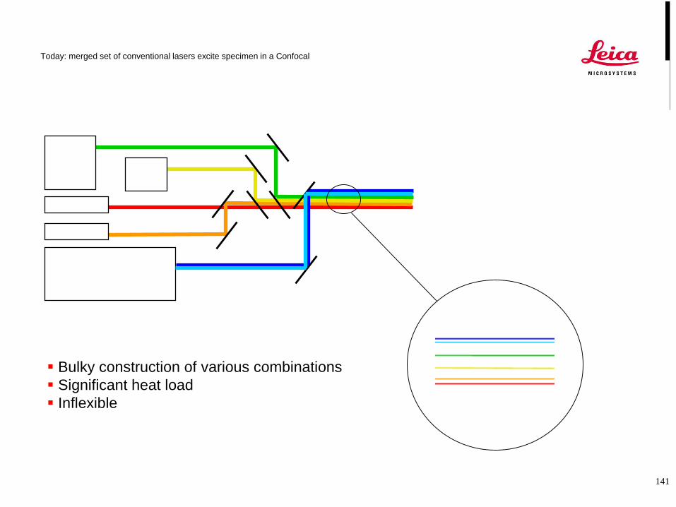
Today: merged set of conventional lasers excite specimen in a Confocal
Bulky construction of various combinations
Significant heat load
Inflexible

142
Tomorrow: SuperK - the White Light Laser
Single solid state device
Adequate output power for imaging
Maintenance free
Low power consumption
Very flexible
Pulsed – FLIM source

143
SuperK laser: Concept
Picosecond Laser
at 1060nm
Seed Source
Pump
Power Amplifier
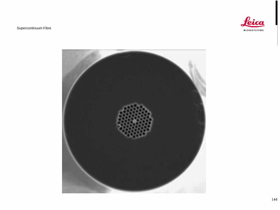
Supercontinuum Fibre
Supercontinuum
Generation
White laser
144
Supercontinuum Fibre

145
Visible spectrum measured with AOTF
0
0,2
0,4
0,6
0,8
1
440 490 540 590 640 690 740
Wavelength (nm)
SuperK laser delivers full spectrum,
has tunable emission
Full tuneability
Optimal excitation
Minimal cross-excitation
450-740 nm range
AOTF
SuperK
Ilklk
n = 1..8

146
SuperK laser: free tuning of up to 8 lines
simultaneously in intensity and wavelength
Freely tunable excitation
8-channel „dimmer“
THE light source
I
l

147
High Quality Imaging with SuperK
Mouse Fibroblasts, triple staining
Cytoskeletal Protein Excitation Emission
Microtubuli 492 494-556
F-Actin 560 566-632
Vimentin 646 659-800