Embed Size (px)
Citation preview

STATE OF CALIFORNIA DEPARTMENT OF TRANSPORTATION TECHNICAL REPORT DOCUMENTATION PAGE TR0003 (REV. 10/98) 1. REPORT NUMBER
CA03-0272
2. GOVERNMENT ASSOCIATION NUMBER
3. RECIPIENT’S CATALOG NUMBER 5. REPORT DATE
November 2003
4. TITLE AND SUBTITLE
Development of 3D Microwave Imaging Technology for Damage Assessment of Concrete Bridge
6. PERFORMING ORGANIZATION CODE
7. AUTHOR(S)
Maria Q. Feng, Franco De Flaviis, Yoo Jin Kim, Hyunseok Ko, and Sunan Liu
8. PERFORMING ORGANIZATION REPORT NO. FHWA/CA/IR/2004/02
10. WORK UNIT NUMBER
9. PERFORMING ORGANIZATION NAME AND ADDRESS
Civil and Environmental Engineering E4120 Engineering Gateway University of California, Irvine Irvine, CA 92697-2175
11. CONTRACT OR GRANT NUMBER
65A0140
13. TYPE OF REPORT AND PERIOD COVERED
Final Report
12. SPONSORING AGENCY AND ADDRESS
California Department of Transportation Division of Research and Innovation, MS-83 1227 O Street Sacramento, CA 95819
14. SPONSORING AGENCY CODE
15. SUPPLEMENTAL NOTES
16. ABSTRACT
An innovative microwave 3-dimensional (3D) sub-surface imaging technology is developed for detecting and quantitatively assessing internal damage of concrete structures. This technology is based on reconstruction of dielectric profile (image) of a structure illuminated with microwaves sent and received by antenna arrays. In this project, it is found that focused microwave is much more effective than the unfocused ones in detecting small defects, and thus a unique numerical bi-focusing technique is developed to focus both the transmitting and the receiving microwave signals. A multi-frequency technique is applied to improve the image clarity by reducing the background noises. Two software packages have been developed in this study: one for 3D image reconstruction and the other for image visualization. Two engineering prototypes have been fabricated: one consists of arrays of 128 antennas and the other 256 antennas with sophisticated electronic switching controlled by software. The first prototype system is tested on concrete blocks, in which voids and steel bars are successfully detected. It was experimentally demonstrated that bi-focusing operator can double the image resolution.
17. KEY WORDS Microwave, Nondestructive Evaluation (NDE), 3D Imaging Technology, Damage Detection
18. DISTRIBUTION STATEMENT No restrictions. This document is available to the public through the National Technical Information Service, Springfield, VA 22161
19. SECURITY CLASSIFICATION (of this report)
Unclassified
20. NUMBER OF PAGES
126
21. PRICE
Reproduction of completed page authorized

Division of Research & Innovation Report CA03-0272 November 2003
Development of 3D Microwave Imaging Technology For Damage Assessment of Concrete Bridge
Final Report

Development of 3D Microwave Imaging Technology For Damage Assessment of Concrete Bridge
Final Report
Report No. CA03-0272
November 2003
Prepared By:
Department of Civil and Environmental Engineering University of California, Irvine
Irvine, CA 92697-2175
Prepared For:
California Department of Transportation Division of Research and Innovation, MS-83
1227 O Street Sacramento, CA 95814

DISCLAIMER STATEMENT
This document is disseminated in the interest of information exchange. The contents of this report reflect the views of the authors who are responsible for the facts and accuracy of the data presented herein. The contents do not necessarily reflect the official views or policies of the State of California or the Federal Highway Administration. This publication does not constitute a standard, specification or regulation. This report does not constitute an endorsement by the Department of any product described herein. For individuals with sensory disabilities, this document is available in Braille, large print, audiocassette, or compact disk. To obtain a copy of this document in one of these alternate formats, please contact: the Division of Research and Innovation, MS-83, California Department of Transportation, P.O. Box 942873, Sacramento, CA 94273-0001.

FINAL REPORT TO
THE CALIFORNIA DEPARTMENT OF TRANSPORTATION
Development of 3D Microwave Imaging Technology
For Damage Assessment of Concrete Bridge
65A0140
Maria Q. Feng, Professor Franco De Flaviis, Assistant Professor
And
Yoo Jin Kim, Post Graduate Researcher Hyunseok Ko, and Sunan Liu, Graduate Research Assistants
DEPARTMENT OF CIVIL AND ENVIRONMENTAL ENGINEERING
UNIVERSITY OF CALIFORNIA, IRVINE
PRINTED NOVEMBER 2003

STATE OF CALIFORNIA ⋅ DEPARTMENT OF TRASPORTATION
TECHNICAL REPORT DOCUMENTATION PAGE TR0003 (REV. 9/99)
1. REPORT NUMBER FHWA/CA/IR/2004/02
2. GOVERNMENT ASSOCIATION NUMBER 3. RECIPIENT’S CATALOG NUMBER
5. REPORT DATE
November, 2003 4. TITLE AND SUBTITLE
Development of 3D Microwave Imaging Technology for Damage Assessment of Concrete Bridge
6. PERFORMING ORGANIZATION CODE
UC Irvine
7. AUTHOR
Maria Q. Feng, Franco De Flaviis, Yoo Jin Kim, Hyunseok Ko, and Sunan Liu
8. PERFORMING ORGANIZATION REPORT NO.
10. WORK UNIT NUMBER
9. PERFORMING ORGANIZATION NAME AND ADDRESS
Civil and Environmental Engineering E4120 Engineering Gateway University of California, Irvine Irvine, CA 92697-2175
11. CONTACT OR GRANT NUMBER
65A0140
13. TYPE OF REPORT AND PERIOD COVERED
Final Report 12. SPONSORING AGENCY AND ADDRESS
California Department of Transportation (Caltrans) Sacramento, CA
14. SPONSORING AGENT CODE
15. SUPPLEMENTARY NOTES
16. ABSTRACT
An innovative microwave 3-dimensional (3D) sub-surface imaging technology is developed for detecting and quantitatively assessing internal damage of concrete structures. This technology is based on reconstruction of dielectric profile (image) of a structure illuminated with microwaves sent and received by antenna arrays. In this project, it is found that focused microwave is much more effective than the unfocused ones in detecting small defects, and thus a unique numerical bi-focusing technique is developed to focus both the transmitting and the receiving microwave signals. A multi-frequency technique is applied to improve the image clarity by reducing the background noises. Two software packages have been developed in this study: one for 3D image reconstruction and the other for image visualization. Two engineering prototypes have been fabricated: one consists of arrays of 128 antennas and the other 256 antennas with sophisticated electronic switching controlled by software. The first prototype system is tested on concrete blocks, in which voids and steel bars are successfully detected. It was experimentally demonstrated that bi-focusing operator can double the image resolution. 17. KEYWORDS
Microwave, Nondestructive Evaluation (NDE), 3D Imaging Technology, Damage Detection
18. DISTRIBUTION STATEMENT
No restrictions.
19. SECURITY CLASSIFICATION (of this report)
Unclassified 20. NUMBER OF PAGES 21. COST OF REPORT CHARGED

DISCLAIMER: The opinion, findings, and conclusions expressed in this publication are those of the authors and not necessarily those of the STATE OF CALIFORNIA

i
Contents
List of Figures .................................................................................................................... iii
List of Tables ..................................................................................................................... vi
Acknowledgement ............................................................................................................ vii
Abstract ............................................................................................................................ viii
1. Introduction....................................................................................................................1
1.1. Problem Statement..................................................................................................1
1.2. Review of the State of the Art ................................................................................3
1.3. Research Objective .................................................................................................7
2. Overview of the Proposed Microwave Imaging Technology ........................................8
2.1. Overview.................................................................................................................8
2.1.1. Surface-Focused Imaging Technology ........................................................9
2.1.2. Sub-Surface-Focused Imaging Technology...............................................10
2.2. Previous Related Works .......................................................................................11
3. Software Development.................................................................................................15
3.1. Image Reconstruction Algorithm and Software ...................................................15
3.2. Study of Image Resolution ..................................................................................19
3.3. Multi-Frequency Technique .................................................................................20
3.4. Visualization Software..........................................................................................22
4. Hardware Development ...............................................................................................23
4.1. Prototype I ............................................................................................................23
4.1.1. Antenna Array Prototype I.........................................................................23
4.1.1.1. Single-Slot Antenna Element............................................................24
4.1.1.2. 16×8 Antenna Array .........................................................................26
4.1.2. Control Module for Prototype I .................................................................29
4.2. Prototype II ...........................................................................................................30

ii
4.2.1. Antenna Array Prototype II .......................................................................31
4.2.1.1. Single-Slot Antenna Element............................................................31
4.2.1.2. PIN Diodes........................................................................................34
4.2.1.3. 4×4 Antenna Array ...........................................................................36
4.2.1.4. 16×8 Antenna Array .........................................................................43
4.2.2. System Integration .....................................................................................49
4.2.2.1. Construction of Measurement Matrix...............................................50
4.2.2.2. Components Details ..........................................................................51
4.2.2.3. Control Program................................................................................53
4.2.2.4. Measurement Speed Evaluation........................................................56
5. Numerical Simulation ..................................................................................................57
5.1. Effective Focusing Area (EFA) ............................................................................57
5.2. Simulation Results Using 5.2 GHz.......................................................................58
5.3. Simulation Results Using 10.0 GHz.....................................................................64
6. Experimental Verification............................................................................................66
6.1. Microwave Imaging Using Prototype I ................................................................66
6.1.1. Experimental Setup....................................................................................66
6.1.2. Experimental Results .................................................................................68
7. Operators Manual of Imaging System .........................................................................71
8. Summary and Concluding Remarks ............................................................................76
Nomenclature.....................................................................................................................77
References..........................................................................................................................78
A. Appendix A: Reference Manual of Modules ...............................................................80
B. Appendix B: Manual of Image Reconstruction Program ............................................87
C. Appendix C: Manual of Control Program ...................................................................99

iii
List of Figures
Figure 1.1 Void and performance degradation ....................................................................3
Figure 1.2 Infrared Image Indicating Voids of a Jacketed Column.....................................6
Figure 2.1 Reflection Mechanisms in RC Column..............................................................9
Figure 2.2 Use of Dielectric Lens to Focus Waves on Bonding Interface ........................10
Figure 2.3 Use of Microwave Arrays to Focus Waves on Sub-Surface Point...................11
Figure 2.4 Designed Dielectric Lenses ..............................................................................12
Figure 2.5 Experimental Setup ..........................................................................................12
Figure 2.6 Typical Responses Using S11 measurement .....................................................13
Figure 2.7 Scanned Microwave Image of Concrete Column Showing Debonding...........13
Figure 3.1 Electromagnetic Compensation Principle ........................................................16
Figure 3.2 Imaging Geometry............................................................................................17
Figure 3.3 Resolution of the system (25mm) at 5.2GHz ...................................................20
Figure 3.4 Comparison of Single/Multi Illuminating Frequency (Image of Two Point-like
Objects) ..............................................................................................................................21
Figure 3.5 Example Screen Shot of Visualization Software..............................................22
Figure 4.1 Two-Dimensional Planar Rectangular Microwave Antenna Array .................24
Figure 4.2 Geometry of Single-Slot Antenna ....................................................................25
Figure 4.3 Measurement Result of Single-Slot Antenna Element .....................................26
Figure 4.4 Fabricated Two-Dimensional Antenna Array ..................................................27
Figure 4.5 Measurement Results of 16×8 Antenna Array .................................................28
Figure 4.6 Switch Box and Power Supply (Manual Operation) ........................................29
Figure 4.7 Description of Three-Dimensional Imaging System (Block Diagram)............30
Figure 4.8 Structures and Dimension of Single-Slot Antenna Element ............................31
Figure 4.9 Single-Slot Antenna Element ...........................................................................32
Figure 4.10 Comparison Between Simulation and Measurement Result ..........................32
Figure 4.11 Radiation Pattern of Slot Antenna..................................................................33
Figure 4.12 Test and De-embedding Fixture ....................................................................34
Figure 4.13 Measurement Comparisons of PIN Diodes ....................................................35
Figure 4.14 Dimension of PIN Diode (MPP-4203) ...........................................................35

iv
Figure 4.15 Fabricated 4 by 4 Antenna Array ...................................................................36
Figure 4.16 Layout of Ground ...........................................................................................37
Figure 4.17 Switching Behavior of Antenna .....................................................................37
Figure 4.18 Comparison Between Simulation and Measurement .....................................38
Figure 4.19 With & Without Diodes..................................................................................38
Figure 4.20 Measurement Set-Up for Insertion Loss.........................................................39
Figure 4.21 Horn Antenna Dimension...............................................................................39
Figure 4.22 Measurement Result .......................................................................................40
Figure 4.23 Complete Slot Antenna Array ........................................................................41
Figure 4.24 Measurement of Each Antenna Element ........................................................42
Figure 4.25 Final Array with Feed Network and Bias Lines.............................................44
Figure 4.26 Final Array with Slots ....................................................................................45
Figure 4.27 Original Layout ..............................................................................................46
Figure 4.28 Simulation Result ...........................................................................................46
Figure 4.29 Solution I ........................................................................................................47
Figure 4.30 Simulation Result ...........................................................................................47
Figure 4.31 Entire Array with Solution I ...........................................................................47
Figure 4.32 Simulation Result ...........................................................................................47
Figure 4.33 Solution II.......................................................................................................48
Figure 4.34 Simulation Result ...........................................................................................48
Figure 4.35 Overall Array with Solution II .......................................................................48
Figure 4.36 Simulation Result ...........................................................................................48
Figure 4.37 Integrated System with Control Rack, Laptop, and Network Analyzer.........49
Figure 4.38 Schematic of Algorithm for System Integration ............................................50
Figure 4.39 Demo Model of 1:128 Switch ........................................................................51
Figure 4.40 Texas Instruments Multiplexers CD74HC4051E...........................................52
Figure 4.41 1:8 Switch.......................................................................................................52
Figure 4.42 Practical Model of 1:128 Switch ....................................................................53
Figure 4.43 Measurement of Data Through Network Analyzer ........................................54
Figure 4.44 Execution of Imaging Program after Measurement .......................................54
Figure 4.45 Panel Interface ................................................................................................55

v
Figure 4.46 Measurement Time Shown in Oscilloscope ...................................................56
Figure 5.1 Effective focusing area of planar rectangular antenna array ............................58
Figure 5.2 Simulation Results with Descriptions ..............................................................63
Figure 5.3 Resolution Improvement Using Higher Frequency..........................................65
Figure 6.1 Experimental Setup ..........................................................................................67
Figure 6.2 Description of Calibration Scheme ..................................................................68
Figure 6.3 Reconstructed Image of Case 1 ........................................................................69
Figure 6.4 Reconstructed Image of Case 2 ........................................................................70
Figure 6.5 Reconstructed Image of Case 3 ........................................................................70
Figure 7.1 Job Flow of the System ....................................................................................71
Figure 7.2 Block Diagram of the System...........................................................................72
Figure 7.3 Outside View of the System.............................................................................72
Figure 7.4 Front Panel of Control Module........................................................................74
Figure 7.5 Example Screen Shot of Visualization Software..............................................75
Figure A.1 Schematic of Algorithm...................................................................................81
Figure A.2 Practical Model of 1:128 Switch .....................................................................82
Figure A.3 Communication Between LabJack and Network Analyzer.............................83
Figure A.4 Element of Measurement Matrix Corresponding to the Number of Element in
Antenna Array....................................................................................................................84
Figure A.5 Interface of LabView.......................................................................................85
Figure A.6 Photo of LabJack .............................................................................................85
Figure A.7 Using the LabJack with Enable Line and Address Line..................................86
Figure A.8 Truth table of MAX396...................................................................................86
Figure C.1 Hierarchy of the LabView program ‘caltrans.vi’.............................................99

vi
List of Tables
Table 1.1 Evaluation of Established Methods ....................................................................6
Table 6.1 Descriptions of Cases for Experimental Study ..................................................66

vii
Acknowledgement
The project was supported by California Department of Transportation under Award No.
65A0140. The authors would like to thank the project managers, Mr. Rosme Aguilar and
Mr. Stephen Sahs with Caltrans, for their supervision, encouragement and support.
Professor Luis Jofre at Technical University of Catalonia, Barcelona, Spain, provided
technical advice regarding imaging algorithm and antenna design.

viii
Abstract
An innovative microwave 3-dimensional (3D) sub-surface imaging technology is
developed for detecting and quantitatively assessing internal damage of concrete
structures. This technology is based on reconstruction of dielectric profile (image) of a
structure illuminated with microwaves sent and received by antenna arrays.
In this project, it is found that focused microwave is much more effective than the
unfocused ones in detecting small defects, and thus a unique numerical bi-focusing
technique is developed to focus both the transmitting and the receiving microwave
signals. A multi-frequency technique is applied to improve the image clarity by reducing
the background noises.
Two software packages have been developed in this study: one for 3D image
reconstruction and the other for image visualization. Two engineering prototypes have
been fabricated, one consists of arrays of 128 antennas and the other 256 antennas with
sophisticated electronic switching controlled by software. The first prototype system is
tested on concrete blocks, in which voids and steel bars are successfully detected. It was
experimentally demonstrated that bi-focusing operator can double the image resolution.

1
Chapter 1
INTRODUCTION
1.1. Problem Statement
This research intended to target the following problems associated with concrete
bridges.
Problem 1: Assessment of internal damage in concrete bridges
Statistics have shown that one third of the nation’s highway bridges are rated
either structurally deficient or functionally obsolete, and many of these bridges will fail to
achieve their design life of fifty to seventy-five years (Dunker and Rabbat, 1990). In
1995, the Federal Highway Administration (FHWA) estimated the cost at approximately
$6 billion per year in the next 25 years to repair and replace these bridges, but the TEA-
21 budget is only at the level of 3 billion per year (FHWA, 1998). It is important, then,
to be able to accurately predict remaining lives of existing bridges by assessing their
structural integrity. Currently, the assessment heavily relies on visual inspections, which
apparently have some limitations. In California, majority of highway bridges are
concrete bridges, and such invisible damage as voids and cracks inside concrete and
debonding between rebars and concrete caused by corrosions, earthquakes, and other
reasons, is of significant concern. Sometimes it is difficult to assess the extent of damage
developed inside the concrete based only on concrete surface cracks.
Problem 2: Detection of damage within concrete structures wrapped with FRP jackets
Recently, FRP composite jacketing has demonstrated its ability to enhance the
confinement and thus to improve the structural integrity of old concrete bridge columns
and girders. The light weight, high strength, and ease of installation make such materials
very practical for retrofitting concrete bridges. Indeed, in California there are an

2
increasing number of bridge columns being strengthened with FRP jackets including
approximately three thousand columns in the most recent retrofit project involving the I-
80 viaduct (Yolo Causeway) in Sacramento-Yolo County.
Despite the proven structural performance of the jacketing retrofit measure and
the large number of bridge columns being retrofitted with FRP jackets, the post-disaster
damage of the concrete columns covered by the FRP composites, remains a significant
concern. Such damage includes large concrete cracks, debonding between concrete and
rebars, and debonding between concrete and FRP jackets. Unfortunately, there is no
unintrusive technology available at this moment to detect such invisible damage.
Problem 3: Quality assurance in FRP jacketing
Unlike steel jacketing where grout is pumped to fill gaps between the jacket and
the column at the time of installation, a jacket made of several layers of FRP material is
often manually applied to a concrete structural element, layer by layer, glued with
adhesive epoxy. The bonding quality between the layers of the composite jacket and
between the jacket and concrete is of another significant concern, as it purely depends on
the workmanship. Imperfect bonding condition, particularly the existence of a large area
of voids, can significantly degrade the structural integrity and safety that could otherwise
be attainable by jacketing. This has been demonstrated by the results of the experiment
performed by the PI at UCI (Haroun, et al., 1997). Three identical half-scale circular
bridge columns with lap splices were built. Two of the columns were wrapped with
identical glass-fiber jackets: one was well wrapped with the adhesive epoxy carefully
applied to the entire jacketing area, while the other was poorly wrapped with many voids
in the epoxy layers. Force-displacement envelops from the cyclic loading tests of the
three columns (unwrapped, well wrapped, and poorly wrapped) are shown in Figure 1.1.
The well wrapped column performed excellently by increasing the column ductility
factor from less than two (unwrapped column) to six, while the poorly wrapped with
many voids barely reached the ductility factor of three.

3
Figure 1.1 Void and performance degradation
Therefore, it is very important to assess the bonding condition of the composite
jackets after the jacket is installed, in order to ensure the expected performance of the
jacketed columns. Once detected, the voids in the bonding interface can be eliminated by
injecting epoxy at the time of jacket installation. The same PI has tried the infrared
thermography for this purpose and found it to be ineffective for a thick jacket with low
heat conductivity. In addition, the heat applied to the column for building a
thermographic profiling may change the property of FRP materials especially before the
materials are fully cured.
1.2. Review of the State of the Art
Various NDE techniques have been studied to detect cracks and voids of concrete
and debonding/delaminations between concrete and rebars. Among them, acoustic wave,
X-ray, nuclear-magnetic resonance (NMR), infrared thermography, and ground
penetrating radar (GPR) are mostly effective. Except for the infrared thermography, none
of them, however, has been studied for FRP-retrofitted concrete structures

4
The acoustic/ultrasonic wave detection is based on the difference in wave velocity
when acoustic/ultrasonic waves propagate through different materials. At the boundaries
between materials, the waves are reflected. The damage such as cracks also act as
boundaries. By analyzing the echoes, it is possible to determine the locations of these
boundaries, as well as the materials in each layer. If sufficient data are available, a 2-D
or 3-D image of the reflected wave may be reconstructed. The ultrasonic imaging theory
is largely dependent on ray tracing and not difficult to implement. For reinforced
concrete columns wrapped with steel jackets, acoustic wave method can be effective
because metal conducts sound wave very well. An FHWA-sponsored project has
developed an ultrasonic imaging method to detect cracks in steel bridges (Chase et al.,
1997), and other research projects have demonstrated the potential to detect voids in
concrete using ultrasonic tomography (Olson, et al, 1993), although the results are
influenced by sizes and shapes of aggregates.
The NMR imaging technology is based on the differences in natural resonant
frequencies (in MHz range) in different materials under nuclear excitation. High-
sensitivity receivers receive these signals, and an image of resonant frequency is
reconstructed for each material. Although it is possible for an NMR system to generate
high resolution 3-D images, it is very expensive and difficult to operate when a high
spatial resolution is required. X-ray imaging is, in principle, very similar to the ultrasonic
imaging and is good in penetrating through loose materials. However, X-ray machines
are usually heavy and difficult to use, as X-ray is harmful to human body.
GPR is widely used to detect anomalies in a material. It is built to detect the
boundaries between materials that have different electrical properties, namely, dielectric
constant and conductivity. The basic idea of GPR is very similar to that of the acoustic
ultrasonic system. A GPR transmitter sends a fast electromagnetic (EM) pulse with a
width in the range of nano-seconds. This pulse propagates through materials and gets
reflected at the interfaces between the materials with different electrical properties. The
reflected signal, mixed with the transmitted wave, is received by the receiver. If the
transmitted signal is narrow enough, the reflected pulses, though very weak compared
with transmitted one and distorted due to the loss in the materials, can be identified,
taking advantage of the time separation between the transmitted and received pulses. By

5
converting the time scale to distance scale, the locations of the boundaries are then
determined. Small and reliable devices producing very short pulses (0.2 ns) able to
obtain spatial resolutions in the range of centimeters are been fabricated and used as
single sensors and also as array of sensors for imaging purposes (Mast, et al., 1998). The
GPR system is very effective when used to detect relatively large objects having
appreciable difference in dielectric constant with the host material through which EM
waves propagate with little loss. In fact, GPR was studied for identifying the
delaminations and reinforcing steel rebars in a concrete bridge deck slab (Chase et al.,
1997). However, for the jacketed columns which require deep detection, the traditional,
time domain-based GPR is not particularly effective primarily because the received
signal is heavily contaminated by noise as it propagates.
Infrared thermography has been studied for detecting delaminations on concrete
bridge deck and concrete surface fatigue cracks (Chase et al., 1997), as well as concrete
pavement voids (Weil, 1994). To build a thermographic profile, one heats up, through
the surface, the entire structure with electric lamps or a hair-dryer-like heater, and then
measures the infrared radiation from the structure. At the points where voids or cracks
exist, the thermographic profile will be different from other areas due to the difference in
heat conductance between air and concrete. This PI has worked with the Aerospace
Corporation to use an infrared camera to assess the bonding condition of an FRP-jacketed
column and one of the images is shown in Figure 1.2. The infrared thermography, by
nature, is not very accurate because of the continuous distribution of the heat and the
amplitude-only measurement of the heat signal. It is impossible to detect the radial
location and depth of voids. In addition, it is difficult to use infrared thermography for
deep detection. The heat applied to the column for building a thermographic profile may
change the property of FRP materials especially before the materials are fully cured.

6
Figure 1.2 Infrared Image Indicating Voids of a Jacketed Column
Regarding the established nondestructive evaluation methods, advantages and dis-
advantages are summarized and compared with each other in Table 1.1 (Kim, 2002).
Table 1.1 Evaluation of Established Methods
Technique Applications Advantages Potential Obstacles to Implementation
Acoustic imaging (Ultrasonic, impact echo and acoustic emission)
Location of voids Not affected by the reinforcement
Long data acquisition process
Highly sensitive to the aggregate size
Infrared thermography Location of cracks,
voids, and delaminations
Easy to apply
No depth information Sensitive to
environmental conditions
No deep detection Heat affects FRP bond
curing
GPR Location of
reinforcement, voids and cracks
Rapid and non-contact measurement and imaging of large area
Limited algorithms in imaging concrete
High attenuation of EM waves in moisture
Total reflection from metals
Radiography & Radioactive tomography
Location of reinforcement, voids and cracks
High resolution images due to the use of non-diffracting sources (X-ray) with high penetrating capability
Expensive and dangerous
Time consuming Accessibility to both
sides of the object required

7
1.3. Research Objective
The primary objective of this project is to develop a portable 3D microwave
imaging technology using antenna arrays for nondestructive evaluation of internal and
invisible damage in reinforced concrete bridge members with and without FRP composite
jackets. Targeted damage includes air voids, cracks, rebar de-bonds, and FRP jacket de-
bonds due to poor installation workmanship and earthquakes.

8
Chapter 2
OVERVIEW OF THE PROPOSED MICROWAVE
IMAGING TECHNOLOGY
2.1. Overview
The proposed microwave imaging technology is based on the analysis, in time
and frequency domains, of a continuous microwave sent toward and reflected from a
layered medium. It is well known that when a plane electromagnetic (EM) wave
launched from an illuminating device (typically an antenna or a lens) toward a layered
medium encounters a dielectric interface, a fraction of the wave energy is reflected while
the rest is transmitted into the medium.
In the case of a RC column wrapped with a layer of FRP jacket subjected to the
incoming wave as shown in Figure 2.1, the first reflection (#1) occurs at the surface of
the jacket, while the second (#2) at the interface between the jacket and the adhesive
epoxy, and the third (#3) at the interface between the adhesive epoxy and the concrete,
assuming the jacket is perfectly bonded to the column without a void or debonding. In
addition, reflections from the interface between the concrete and steel reinforcing rebars
and from the sources internal to the illuminating device will also take place. If there is an
air gap resulting from a void or debonding between the composite jacket and the column,
an additional reflection (#4) will occur at this particular location, as illustrated in Figure
2.1. Therefore, imperfect bonding conditions can be, in principle, detected by analyzing
these reflections in the time and/or in the frequency domains.

9
#4
#1
#2 #1
#2
Jacket Air Gap Epoxy
#3#3
With air gap Without air gap
Concrete
Figure 2.1 Reflection Mechanisms in RC Column
Based on the numerical studies performed by the authors, focused microwave is
much more effective than the conventional un-focused microwave for detecting small
defects (Feng et al., 2002). The authors proposed two innovative techniques for focusing
microwaves: one using dielectric lenses (referred to as surface-focused imaging
technology and the other using antenna array (referred to as sub-surface-focused imaging
technology).
2.1.1. Surface-Focused Imaging Technology
The surface-focused microwave imaging technology is proposed for assessing
damage not too deep below the structure surface, such as internal voids near the surface
and debonding between concrete and FRP jackets. Previous work by this proposal team
demonstrated that the plane EM wave is not effective in detecting such voids and
debonding, as the reflection contribution of the voids and debonding is very small
compared to that from the concrete structure itself. In order to overcome the difficulty
associated with the plane EM wave, the use of a dielectric lens was invoked to focus the
EM wave on the bonding interface of the jacketed column while diffusing the field in
other regions of no interest, as illustrated in Figure 2.2. Waves reflected from the other
regions where the beam is defocused will be much weaker than those from the focused
region, and thus the difference between the perfect and poor bonding conditions in the
focused region can be detected more effectively.
10
Defocused Wave(Weak Interaction)
Concrete Column
Steel RebarsFRP Jacket
Focusing Spot
Figure 2.2 Use of Dielectric Lens to Focus Waves on Bonding Interface
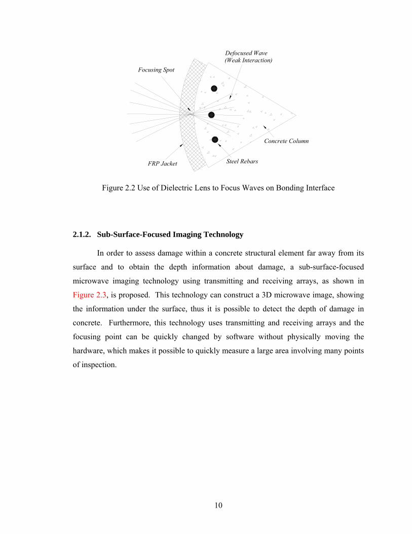
2.1.2. Sub-Surface-Focused Imaging Technology
In order to assess damage within a concrete structural element far away from its
surface and to obtain the depth information about damage, a sub-surface-focused
microwave imaging technology using transmitting and receiving arrays, as shown in
Figure 2.3, is proposed. This technology can construct a 3D microwave image, showing
the information under the surface, thus it is possible to detect the depth of damage in
concrete. Furthermore, this technology uses transmitting and receiving arrays and the
focusing point can be quickly changed by software without physically moving the
hardware, which makes it possible to quickly measure a large area involving many points
of inspection.

11
2.2. Previous Related Works
Under the support of NSF, the proposal team developed the surface-focused
microwave imaging technology and experimentally demonstrated its efficacy in detecting
debonding in FRP-jacketed columns. Dielectric lenses were developed for focusing microwaves onto locations of
interest in concrete structures. Two types of the developed lenses are shown in Figure
2.4: one in triangular and the other in circular shape. They can be setup for the reflection
measurement (S11) (requiring only one lens as shown in Figure 2.5(a)), or the
transmission measurement (S21) (requiring two lenses as shown in Figure 2.5(b)).
Concrete Column
Receiving Arrays
Transmitting Arrays
rf
I r1
I r2
I rm
I tn
I t1I t2
Receiver Focusing Operator on rf
Transmitter Focusing Operator on rf
Focused Point
Figure 2.3 Use of Microwave Arrays to Focus Waves on Sub-Surface Point

12
(a) Circular Lens (b) Triangular Lens
Figure 2.4 Designed Dielectric Lenses
(a) Reflection Measurement (S11) (b) Transmission Measurement (S21)
Figure 2.5 Experimental Setup
The effectiveness of the proposed EM imaging technology using focused EM
waves was investigated through a series of experiments on a variety of concrete specimen
including concrete cubs and FRP-jacketed concrete columns. The concrete cub has 30
cm (11.81 in) in each side and the concrete columns are of 40.64 cm (16 in) in diameter
and 81.28 cm (32 in) in height. Some of these columns were built without reinforcing
rebars and the some with No. 5 longitudinal rebars and No. 2 circular hoops, in order to
examine the influence of steel rebars on the EM wave reflection. Each of the columns
was wrapped with a three-layer glass FRP jacket. Various voids and debonding
conditions were artificially introduced inside the concrete cubs and between the jackets
and the columns of the jacketed columns.
Figure 2.5 shows an experimental setup with the concrete columns respectively
using the triangular and circular lenses. Continuous sinusoidal microwaves with its

13
frequency sweeping from 8.2 GHz to 12.4 GHz were generated from the signal analyzer
and sent to the jacketed columns through the lenses. Typical frequency-domain
responses by S11 measurement using one circular lens are plotted in the Figure 2.6. The
response has been normalized by the reference value representing a perfect bonding
condition. It is shown that the response from the poor bonding condition in Figure 2.6(b)
has a large variance while the one from the good bonding condition in Figure 2.6(a) is
almost zero.
8.0 8.5 9.0 9.5 10.0 10.5 11.0 11.5 12.0 12.5Frequency (GHz)
-15.0-10.0
-5.00.05.0
10.015.0
Nor
mal
ized
Res
pons
e (d
B)
at 350 degree locarion
8.0 8.5 9.0 9.5 10.0 10.5 11.0 11.5 12.0 12.5
Frequency (GHz)
-15.0-10.0
-5.00.05.0
10.015.0
Nor
mal
ized
Res
pons
e (d
B)
at 0 degree location
(a) Response from Good Bonding Condition (b) Response from Poor Bonding Condition
Figure 2.6 Typical Responses Using S11 measurement
Figure 2.7 shows a scanned image of a column surface area. This area contains a
void between the jacket and the column caused by a hole with a diameter of
approximately 2 cm in the concrete column surface. Although the air void cannot be seen
from the outside of the jacket, the scanned microwave images clearly identify the location
and size of the void.
Figure 2.7 Scanned Microwave Image of Concrete Column Showing Debonding
Measuring Point (mm)
Measuring Point (mm)
S21/Ref. (dB)

14
From the experimental results, it is demonstrated that the surface-focused imaging
technology can successfully detect the location and size of voids in concrete structures
with and without FRP jackets. Accurate information about the void’s depth, however,
cannot be easily obtained.

15
Chapter 3
SOFTWARE DEVELOPMENT
3.1. Image Reconstruction Algorithm and Software
From the electromagnetic point of view, nondestructive evaluation in civil
engineering can be confronted with the identification of dielectric inhomogeneities (as air
void or steel rebar) inside homogeneous dielectric materials (as concrete or FRP). For
the reconstruction or imaging of these defects, an illumination field has to be applied,
propagating uniformly through the medium. When the illumination field reaches the
defects, the uniformity will be lost and a disturbance on the existing field, generally
called total field (Et) as represented in Figure 3.1(a), will be created. In order to model
this situation following the electromagnetic compensation principle (Harrington, 1961),
the inhomogeneities can be replaced by an equivalent electric current distribution:
tmediaobjeq j EJ )( εεω −= (3.1)
where εobj and εmedia are permittivity of the object and the homogeneous surrounding
medium respectively. These currents can also be treated as the source of a scattered field
Es (Es = Et − Ei) placed inside a homogeneous medium in Figure 3.1(b):
dVe jk
V eqs rJE
r
π4
−
∫= (3.2)
When the electric contrast (based on the difference of permittivity and the size of
the defect in terms of wavelengths) between the defects and the homogenous surrounding
medium is low enough, the disturbances created on the propagating field by these
inhomogeneities can be considered small, and the total field can be approximated by the
initial incident field (Et ≈ Ei). The equivalent electric current distribution, therefore, can
also be approximated by:
imediaobjeq j EJ )( εεω −= (3.3)

16
(a) Illumination of Object
(b) Equivalent Electric Current Distribution to Object
Figure 3.1 Electromagnetic Compensation Principle
This approximation (Slaney et al., 1984) is called the first-order Born
approximation and it simplifies enormously the inverse reconstruction procedure. In
order to obtain an image of the object (internal dielectric inhomogeneities in the case)
from external measurements, the reconstruction of a current distribution Jeq from the
scattered field measured over a certain wrapping surface can be the replica of the object.
The current distribution is able to be obtained from the inversion of the integral equation
(2).
The geometry of imaging is shown in Figure 3.2, where the transmitting surface
array is able to sequentially focus on every interrogation point of the reconstructing
volume while the receiving surface array measures the scattered field enveloping the
object. The measurement geometry uses Nk × Nl elements forming a transmitting array
and Nm × Nn elements forming a receiving array. In the measurement, an Nt × Nr
measurement matrix, where Nt = Nk × Nl is the total numbers of transmitting elements and
Jeq
εmedium Es
εobject Object
εmedium
Ei
Et

17
Nr = Nm × Nn is the total numbers of receiving elements, can be obtained as follows: for
every selected transmitting element, the receiving array is scanned obtaining an Nr-
measurement column, then the procedure is repeated for the rest of the Nt transmitting
elements.
Transmitting Surface Array(N k x N l)
Receiving Surface Array(N m x N n)
Reconstruction CellDefect/Object
Reconstruction Volume
ro
rfEiEs
rT,klrR,mn
Figure 3.2 Imaging Geometry
The image reconstruction algorithm forms a point image by means of
synthesizing the two focused arrays (transmitting and receiving arrays). All the elements
of the arrays are weighted by a focusing operator so as to be focused on a unique point,
which can be achieved by a numerical treatment of the measurement matrix. The
focusing operator (Broquetas et al., 1991) can be obtained by taking an inverse of the
field induced by a current point source. It is well known that the electric fields of the
point electric source are proportional to the Green’s function, e-jkr/4πr, while the electric
fields are proportional to a Hankel function of the second kind whose argument is
proportional to the distance from the source to the observation point in 2-dimensional
space (Balanis, 1989). Therefore, the incident field at ri=(xi,yi,zi) when focusing from
every transmitting point rTkl=(xTkl,yTkl,zTkl) on the reconstructing point rf=(xf,yf,zf) can be
expressed as
∑∑= =
−−
−⋅=
l k iTkleN
l
N
k iTkl
jk
fTkliieIE
1 1
||
||4)()(
rrrr
rr
π (3.4)
where ITkl(rf), the focusing operator, is given by

18
||
||4)(
fTklejkfTkl
fTkl eI rr
rrr −−
−=
π (3.5)
where re kk ε0= . The concrete was assumed to be homogeneous having uniform
dielectric constant εr=5.3 for the purpose of computational ease (Feng et al., 2002).
Scattered field measured at rRmn=(xRmn,yRmn,zRmn) of a defect placed at r0=(x0,y0,z0)
can be expressed as following the Eq. (3.2).
dVeIEERmn
jk
V objiRmns
Rmne
||4)()(
0
||
0
0
rrrr
rr
−⋅⋅=
−−
∫ π (3.6)
where Iobj is a constant for every object containing its electromagnetic macroscopic
characteristics.
When focusing back the received field at rRmn=(xRmn,yRmn,zRmn) on the interest
point rf=(xf,yf,zf), electromagnetic image of Ef at rf=(xf,yf,zf) can be expressed as
∑∑= =
⋅=n mN
n
N
mfRmnRmnsff IEE
1 1)()()( rrr (3.7)
where IRmn(rf), the focusing operator, is given by
||
||4)(
fRmnejkfRmn
fRmn eI rr
rrr −−
−=
π (3.8)
Finally, all the processes can be grouped as follows:
∑∑ ∫ ∑∑= = = =
−−−−
⎥⎥⎦
⎤
⎢⎢⎣
⎡
⎭⎬⎫
⎩⎨⎧
−⋅⋅
−⋅⋅=
n m l k TkleRmneN
n
N
mV
N
l
N
k Tkl
jk
fTklRmn
jk
objfRmnff dVeIeIIE1 1 1 1 0
||
0
||
||4)(
||4)()(
00
rrr
rrrr
rrrr
ππ (3.9)
In order to express Eq. (3.9) as a matrix form including the measurement matrix,
the index of transmitting and receiving array can be arranged as follows:
TtTkl rr → for transmitting array (3.10)
where subscript t is from 1 to the maximum number of transmitting element, and
RrRmn rr → for receiving array (3.11)
where subscript r is from 1 to the maximum number of receiving element.

19
Then, the matrix form can be expressed as follows:
[ ]⎥⎥⎥⎥
⎦
⎤
⎢⎢⎢⎢
⎣
⎡
⋅
⎥⎥⎥⎥
⎦
⎤
⎢⎢⎢⎢
⎣
⎡
⋅=
Rr
R
R
RTsRTsRTs
RTsRTsRTs
RTsRTsRTs
TtTTff
I
II
EEE
EEEEEE
IIIEΜ
ΛΜΟΜΜ
ΛΛ
Λ 2
1
11,11,11,
11,11,11,
11,11,11,
21)(r (3.12)
Finally, a 3D image of a volume can be generated based on the image Ef at each
interrogation (focusing) point within the reconstructing volume.
3.2. Study of Image Resolution
The image reconstruction algorithm developed in the previous section was applied
to the case of two (transmitting and receiving) arrays each consisting of 128 (8×16)
antennas, with the frequency of 5.2 GHz, while the wavelength in concrete, λe, is 25.06
mm. Numerical simulations using analytical measurement data were conducted in order
to verify the resolution capability of the system. Two point-like objects were placed with
the distance of 25.0 mm along each axis at the center of the reconstructing volume. As
shown in Figure 3.3, the results demonstrated that the system, due to the use of bi-
focusing (focusing both the transmitting and receiving arrays), is able to achieve a
resolution in the order of the wavelength in the dielectric medium, which is 25.0 mm at
5.2 GHz in concrete.

20
(a) X-direction (b) Y-direction (c) Z-direction
Figure 3.3 Resolution of the system (25mm) at 5.2GHz
3.3. Multi-Frequency Technique
In order to improve the quality of reconstructed image by reducing the
background noises, a narrow band multi-frequency technique was applied. In this
technique, three or four microwaves with frequencies near the designed illuminating
frequency was sent from and received by the antenna arrays. By averaging the images
reconstructed from the waves of different frequencies, background noise including the
steel interference can be averaged out and the object image can be amplified to improve
the signal-to-noise ratio. This technique has been used with some success for similar
problems (Pierri et al., 2000, Bucci et al., 2000).
According to the sweeping of frequency, both incident/scattered field and
numerical focusing operator become a function of frequency:
, ,
( ) ( , )( ) ( , )( ) ( , )
( ) ( , )
i i i i eN
s sRmn Rmn eN
eNf f f f
eNTkl Rmn f Tkl Rmn f
E E kE E kE E kI I k
→→→
→
r rr rr r
r r
(3.13)
where eNk , the effective wave number at the Nth frequency.
Then, the electromagnetic image of fE at ( , , )f f f fx y z=r can be expressed as
00 | || |
1 1 10 01 1
( , )
( )( , )| | | |
n ml k eNeN Rmn Tkl
Rmn eNfNFreq N N
N N jkjkf f
N n m eNobj Tkl fV Rmn Tkll k
I k
E e eI I k dV− −− −
= = == =
⎡ ⎤⎢ ⎥⎢ ⎥⎧ ⎫⎢ ⎥⎪ ⎪
⎨ ⎬⎢ ⎥⎪ ⎪⎢ ⎥⎩ ⎭⎣ ⎦
⋅
=⋅ ⋅
− −∑ ∑∑ ∑∑∫
r rr r
r
rrr r r r
(3.14)
or
, 1 1 , 1 2 , 1 1, 2 1 , 2 2 , 2 2
1 21
,, 1 , 2
( )
s T R s T R s T Rr RNFreqs T R s T R s T Rr R
TtT Tf fN
Rrs TtRrs TtR s TnR
E E E IE E E IE I I I
IE E E=
⎡ ⎤ ⎡ ⎤⎢ ⎥ ⎢ ⎥⎢ ⎥ ⎢ ⎥⎡ ⎤ ⎢ ⎥⎣ ⎦ ⎢ ⎥⎢ ⎥ ⎢ ⎥⎢ ⎥ ⎢ ⎥⎣ ⎦⎢ ⎥⎣ ⎦
= ⋅ ⋅∑r
LL
L MM M O ML
(3.15)
where NFreq is the number of frequencies used.
21
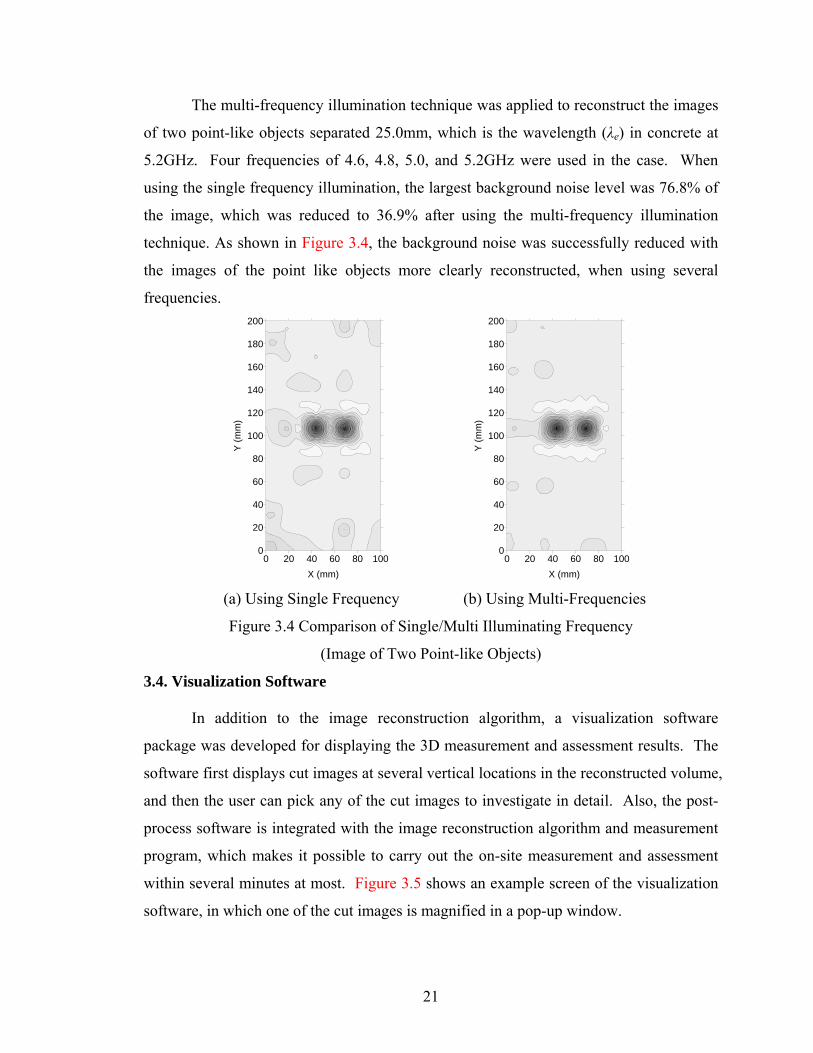
The multi-frequency illumination technique was applied to reconstruct the images
of two point-like objects separated 25.0mm, which is the wavelength (λe) in concrete at
5.2GHz. Four frequencies of 4.6, 4.8, 5.0, and 5.2GHz were used in the case. When
using the single frequency illumination, the largest background noise level was 76.8% of
the image, which was reduced to 36.9% after using the multi-frequency illumination
technique. As shown in Figure 3.4, the background noise was successfully reduced with
the images of the point like objects more clearly reconstructed, when using several
frequencies.
0 20 40 60 80 100X (mm)
0
20
40
60
80
100
120
140
160
180
200
Y (m
m)
0 20 40 60 80 100
X (mm)
0
20
40
60
80
100
120
140
160
180
200
Y (m
m)
(a) Using Single Frequency (b) Using Multi-Frequencies
Figure 3.4 Comparison of Single/Multi Illuminating Frequency
(Image of Two Point-like Objects)
3.4. Visualization Software
In addition to the image reconstruction algorithm, a visualization software
package was developed for displaying the 3D measurement and assessment results. The
software first displays cut images at several vertical locations in the reconstructed volume,
and then the user can pick any of the cut images to investigate in detail. Also, the post-
process software is integrated with the image reconstruction algorithm and measurement
program, which makes it possible to carry out the on-site measurement and assessment
within several minutes at most. Figure 3.5 shows an example screen of the visualization
software, in which one of the cut images is magnified in a pop-up window.

22
(a) Several Cut Images along Z-Axis
(b) Magnified Image at Z=0 mm
Figure 3.5 Example Screen Shot of Visualization Software

23
Chapter 4
HARDWARE DEVELOPMENT
4.1. Prototype I
4.1.1. Antenna Array for Prototype I
Prototype I consists of 128 antenna elements placed in two 8 × 8 matrices. As
illustrated in Figure 4.1, the planar rectangular microwave antenna is composed of
transmitting and receiving arrays, each consisting of 8 × 8 slot antennas. Each of these
two planar 8 × 8 arrays consists of a parallel fed 8-element vertical array producing a
tomographic focused slice perpendicular to the vertical axis of the structure, and an
electronically switched 8-element horizontal array able to focus on a particular point
inside the previous tomographic focused slice. The transmitting antenna array focuses
the illuminating fields on a particular point inside the volume of investigation and the
receiving array focuses the receiving beam on the same point. The whole antenna is a
sandwich structure with two metallic grounded substrates separated by a light foam layer.
The grounded substrate close to the target concrete structure contains the radiating half-
wavelength (λ/2) slots in the exterior ground plane and the 100 Ω microstrip feeding line
on the interior side. The second grounded plane, quarter-wavelength (λ/4) apart from the
slot plane, acts as a reflector in order to produce a unidirectional radiation towards the
volume of investigation.
An illuminating frequency of 5.2GHz was chosen as it represents a reasonable
tradeoff between the signal attenuation and the image resolution. Due to the use of the bi-
focusing technique, an image resolution of 2.5cm can be achieved at 5.2GHz, which is
the wavelength (λe) in concrete.
A microstrip slot antenna was chosen in order to be directly attached to the
concrete surface or the matching cushion. The microstrip slot antenna has the advantage
of being able to produce either bi-directional or unidirectional radiation patterns with a
large bandwidth. The strip and slot combination offers an additional degree of freedom in
the design of the microstrip antenna (Garg et al., 2001).

24
At last, the geometry of the slot antenna was determined so as to obtain a wide
bandwidth at the resonance frequency of 5.2GHz. The number of antennas (128) and the
antenna array dimension of 20cm×20cm were selected as they represent a reasonable
tradeoff between the resolution and the reconstructed area covered by the antenna array.
Transmitting ArrayReceiving Array
Attach to Objectto be Investigated
λ/2 Slot
Microstrip Feed
Reflector (Steel)λ/4
1.25 cm20 cm
2.5
cm17
.5 c
m
(a) Conceptual Design of Planar Rectangular Slot Antenna Array
(b) Eight Elements Linear Array with Corporate Feed Configuration
Figure 4.1 Two-Dimensional Planar Rectangular Microwave Antenna Array
4.1.1.1. Single-Slot Antenna Element
Prior to the antenna array design, a single-slot antenna was designed and
simulated using Ansoft High Frequency Structure Simulator (HFSS). The geometry of
the single-slot antenna is described in Figure 4.2.
100 Ω
71 Ω 100 Ω
71 Ω 100 Ω 100 Ω
50 Ω

25
25 m
m
17 m
m
2 mm
0.7
mm
2.35 mm
10.6
5 m
m
Slot
Microstrip Feed
100 Ω Impedance
Ls
Lm
Ws
W
(a) Geometry of Single-Slot and Microstrip Feed
(b) Geometry of Substrates and Foam
Figure 4.2 Geometry of Single-Slot Antenna
As shown in Figure 4.2, a dimension of 12.5 mm ×25 mm is assigned for each
slot. This limitation of the size forces the microstrip feed to be bended. The important
factors that can affect the resonance frequency and bandwidth are the length of microstrip
feed, Lm, and the length of the slot, Ls. These are adjusted to satisfy the resonant

26
frequency around 5.2 GHz and a large bandwidth suggested by the simulation results
using HFSS. The S11 parameter of the designed single-slot antenna is calculated,
renormalized with port characteristic impedance of 50Ω and plotted in Figure 4.3 in the
frequency range from 4 GHz to 7 GHz. The magnitude of S11 at resonance (5.58 GHz) is
-26 dB, the one at 5.2 GHz is -17 dB, and the bandwidth at -10 dB is about 1.5 GHz.
(a) Fabricated Single-Slot Antenna Element
4 4.5 5 5.5 6 6.5 7Frequency (GHz)
-60
-50
-40
-30
-20
-10
0
Mag
nitu
de (d
B)
Single Slot AntennaS11 from MeasurementS11 from Simulation (HFSS)
(b) S11 Parameter of Single-Slot Antenna Calculated Using HFSS (Z0 = 50 Ω)
Figure 4.3 Measurement Result of Single-Slot Antenna Element
4.1.1.2. 16×8 Antenna Array
A significant technical challenge in developing the antenna array is to achieve a
high radiation performance (meaning a larger bandwidth at the illuminating frequency)
and low mutual coupling (meaning low interference among the slot antenna elements).

27
Although numerous studies have been performed by electrical engineers to study
radiation of antenna arrays into air for communication purposes, no literature can be
found regarding design knowledge for concrete-radiation antenna arrays.
The antenna array fabricated in this study was tested using a network analyzer,
measuring reflection parameters (Sii) for investigating the radiation performance and
transmission parameters (Sij) for the mutual coupling. The antenna array was placed on a
concrete block, allowing the wave radiating through the concrete. As plotted in Figure
4.5(a), the magnitude of Sii parameters around 5.2 GHz is less than -10dB, implying that
the antenna achieved high radiation performance. The transmission parameters plotted in
Figure 4.5(b) shows that the interference between the co-lateral elements (array 8 and 9)
is as low as -20 dB, which is acceptable. Therefore, this study achieved a high-
performance antenna array.
(a) 16×8 Slots (b) Coaxial Feeds
Figure 4.4 Fabricated Two-Dimensional Antenna Array

28
5 5.2 5.4 5.6 5.8 6Frequency (GHz)
-30
-25
-20
-15
-10
-5
0
Mag
nitu
de (d
B) Sii of Transmitting Arrays
Array 1Array 2Array 3Array 4Array 5Array 6Array 7Array 8
(a) Sii Measurement of Transmitting Arrays
5 5.2 5.4 5.6 5.8 6Frequency (GHz)
-50
-40
-30
-20
-10
0
Mag
nitu
de (d
B)
Sij MeasurementFrom Array 8 To Array 9
(b) Transmission Measurement (Sij of Array 8 and Array 9)
Figure 4.5 Measurement Results of 16×8 Antenna Array

29
4.1.2. Control Module for Prototype I
For the reason that the antenna array has 16 coaxial feeds, a switch box is
necessary to control the input from and output to the network analyzer. In this study, RF
switches, which can control two outputs from one input in each unit with a control
voltage of 20V, are used and assembled to make the switch box: there are 8 transmitting
ports with one input from the network analyzer, and 8 receiving ports with one output to
network analyzer. Figure 4.6 represents the switch box and a power supply to provide
control voltage.
(a) Switch Box (b) Power Supply
Figure 4.6 Switch Box and Power Supply (Manual Operation)

30
4.2. Prototype II
Prototype II is a much more sophisticated and ambitious system. Compared to
Prototype I, it not only consists of much more antenna elements (256) to cover a larger
inspection volume, but also engages much more sophisticated electronic antenna
switching controlled by software. The system is composed with a control module,
switching unit, antenna array, network analyzer, image reconstruction algorithm, and
display unit. The final product to user is the reconstructed sub-surface image under
testing, the 3D dielectric profiles of the objects in reconstructing volume. The
measurement is performed by electronically switched antenna array and portable network
analyzer, which is also controlled by control module. The block diagram in Figure 4.7,
describes the connectivity and job flow of the system.
Figure 4.7 Description of Three-Dimensional Imaging System (Block Diagram)

31
4.2.1. Antenna Array for Prototype II
4.2.1.1. Single-Slot Antenna Element
The illumination frequency on a working medium of concrete (εr = 5.3) was
chosen as 5.2GHz, which again represents a reasonable trade-off between the image
resolution and the penetration depth. The type of antenna was chosen as a microstrip-fed
single antenna. The entire structure of the slot antenna and its dimension are illustrated in
Figure 4.8. Two layers of 15-mil-thick Duroid 5880 (εr = 2.2, tan δ = 0.0009) are placed
on the top and bottom of the foam. The foam used here is Rohacell Rigid Foam by
Richmond Aircraft Products whose dielectric constant is nearly unity, which resembles
that of air. The thickness of the foam is 12 mm, which is approximately quarter-wave
length if the thickness of the top and bottom dielectrics is included. The substrate has two
sides of 0.5 oz. of copper layer rolled. The antenna is fed by microstrip line that passes
the slot in the middle. The dimension of the microstrip-fed slot antenna was designed
and optimized initially to give the impedance matching to 50 Ω and operate at 5.2 GHz
using Agilent’s Momentum. Then, another simulator called High Frequency Structure
Simulator (HFSS) was used to check that the two different simulators provide similar, if
not identical, results. The width of the microstrip feed was chosen to yield 50 Ω
transmission line.
1.75
1.95
3.25
2.14
Foam
Reflector
SlotFeed
Substrate
1.18
9.64
Figure 4.8 Structures and Dimension of Single-Slot Antenna Element

32
The slot was modeled as “magnetic wall,” which is frequently used to
approximate the holes in electromagnetic simulation. In addition, more boundary
condition such as perfect electric field for the ground plane was applied to reduce the
simulation time. The comparison between simulation result using HFSS and
measurement is shown in Figure 4.10. The plot shows that simulation resonates at 5 GHz
with the return loss of –20 dB while the measurement’s resonant frequency is at 5.2 GHz
with the return loss of –21 dB. Very good consistency between the simulation and
measurement results exist in both resonant frequency and return loss of the antenna. The
-10 dB bandwidths are 13.5% and 11.5% for the simulation and the measurement
respectively.
(a) Slot (b) Microstrip Feed
Figure 4.9 Single-Slot Antenna Element
3.5 4.0 4.5 5.0 5.5 6.0 6.53.0 7.0
-20
-15
-10
-5
-25
0
Frequency (GHz)
Ret
urn
Loss
(dB
)
SimulationMeasurement
Figure 4.10 Comparison Between Simulation and Measurement Result

33
The simulated radiation patterns of different polarization at different cuts are
shown in Figure 4.11. Also, HFSS was used for the simulation. Each plot had been
normalized to its maximum electric field and contains electric fields in both phi and theta
directions. The line with × marks is Ephi and the line with Δ marks represents Etheta. Ephi
at ϕ = 0° is almost negligible, but Ephi is dominant at ϕ =90°.
(a) Ephi and Etheta at ϕ = 0° (b) Ephi and Etheta at ϕ =90°
(c) Ephi and Etheta at θ= 90°
Figure 4.11 Radiation Pattern of Slot Antenna

34
4.2.1.2. PIN Diodes
The individual antenna element in three-dimensional array was designed to be
activated by switching using PIN diodes. Three different types of diodes were evaluated
to find the most suitable diodes; Agilents’ HSMP-389F, HMPP-3895 and Microsemi’s
MPP-4203 come in different packages and material. HSMP-389F is SOT-323 type.
HMPP-3895 is specially packaged in MiniPak® without lead pins but with gold pads at
the bottom. These two diodes are in common cathode configuration. Two PIN diodes
share cathode in one package. HMPP-3895 is smaller. Third diode, MPP-4203, is in
0204 package and therefore the smallest. This diode, however, contains only one diode
in each package.
For the measurement, 50-Ohm microstrip line was fabricated using the same
dielectric used for the antenna with the center of the line open-circuited for diode
mounting. Then, the through-line was de-embedded mathematically for more accurate
measurement. Bias voltage of 0.9 volt was applied to the diode. The test fixture and de-
embedding through line are shown in Figure 4.12.
(a) Test Fixture (b) De-embedding Fixture
Figure 4.12 Test and De-embedding Fixture

35
1 2 3 4 5 6 7 8 90 10
-20
-10
0
-30
10
Frequency (GHz)In
serti
on L
oss
(dB
)
HSMP-389F
HMPP-3895
MPP-4203
Figure 4.13 Measurement Comparisons of PIN Diodes
The measurement results of three different types of diodes are compared in Figure
4.13. The sudden drop in the MPP-4203’s measurement between 6 GHz and 8 GHz
could be removed by performing calibration procedure more carefully. MPP-4203 shows
the most promising isolation at 5 GHz. Although insertion losses are very closely spaced
to each other, MPP-4203 suffers from the lowest insertion loss of all. Insertion loss is 0.3
dB while the isolation is nearly 12 dB.
Figure 4.14 shows the dimension of the MPP-4203. The largest dimension is only
1 mm with the rest being sub-millimeter.
Figure 4.14 Dimension of PIN Diode (MPP-4203)
1 mm
0.5 mm
0.4 mm
Bottom Cathode

36
4.2.1.3. 4×4 Antenna Array
At first, a preliminary 4 by 4 antenna array was fabricated and real diodes were
soldered onto the substrate as shown in Figure 4.15 to verify the simulation results. The
design of the 4×4 antenna array can be directly expanded to the whole array, or can be a
sub-module of the whole array, i.e. the whole array consists of sixteen 4×4 modules.
Figure 4.16 shows the layout of the ground and ground pad. In the middle of the ground
pad, via was created by drilling a hole connecting the via pad to the ground. Only four
PIN diodes were used to turn on one antenna element. Via is located approximately 1
mm above bias line as shown in Figure 4.16. Bias pads were located along the periphery
of the substrate square.
(a) Feed Network with Bias Pads (b) U-shaped Slots
Figure 4.15 Fabricated 4 by 4 Antenna Array

37
9.76
2
1.5
0.2
V i a
Bias Line
Ground Pad
Figure 4.16 Layout of Ground
Figure 4.17 shows two measurements of the array: when all the four diodes are
turned on and off. DC voltage of 3.6 V and 20 mA DC current was applied to the
antenna array. Across each diode, roughly 0.9 V was applied. This bias can turn on four
diodes at the same time, establishing low impedance path to the input port. The resonant
frequency was 4.94 GHz and return loss was –36 dB when all the diodes were turned on.
When they were off, return loss was –0.03 dB at 4.94 GHz. PIN diodes exhibited very
good isolation at off state. The –10 dB bandwidth was approximately 11.3 %.
4.2 4.4 4.6 4.8 5.0 5.2 5.4 5.6 5.84.0 6.0
-30
-20
-10
-40
0
Frequency (GHz)
Ret
urn
Loss
(dB)
OnOff
Figure 4.17 Switching Behavior of Antenna

38
4.2 4.4 4.6 4.8 5.0 5.2 5.4 5.6 5.84.0 6.0
-30
-20
-10
-40
0
Frequency (GHz)
Ret
urn
Loss
(dB
)MeasurementSimulation
Figure 4.18 Comparison Between Simulation and Measurement
Figure 4.18 shows the comparison between the simulation result using
Momentum and measurement. Very good agreement was observed between them.
Simulation result indicates the resonant frequency at 5 GHz with the return loss of
roughly -20 dB. Also, Figure 4.19 compares the array’s return loss when diodes were
applied with bias and microstrip lines replaced the diodes. In the gap where diode was to
be soldered across, a small piece of copper tape was placed. Both lateral and vertical
dimensions of tape resembled that of the diode. The diode’s parasitic capacitance at on
state slightly brought down the resonant frequency of the array.
4.2 4.4 4.6 4.8 5.0 5.2 5.4 5.6 5.84.0 6.0
-30
-20
-10
-40
0
Frequency (GHz)
Ret
urn
Loss
(dB
)
Without diodesWith diodes
Figure 4.19 With & Without Diodes

39
Diodes’ applicability to microwave imaging was also checked. To do so, the set-
up in Figure 4.20 was used to test if the receiving antenna array was able to accept any
power from the transmitting horn antenna or vise versa. A rectangular concrete block
was inserted between the transmitting and receiving antenna with certain dimension. The
broadband receiving horn antenna was verified experimentally that it operates at 5.2 GHz
with concrete block before performing the measurement. The dimension of the horn
antenna used is illustrated in Figure 4.21. Only part of input power that was transmitted
through the horn antenna would be received by the antenna array, more likely activated
antenna element.
25.5 cm
28 cm
3.8 cm
ArrayTransmitter
Horn Antenna(1 GHz - 12.4 GHz)
Receiver
Concrete
ActivatedAntenna Element
Figure 4.20 Measurement Set-Up for Insertion Loss
24.4 cm
14.4 cm
1.5 mm
Horn Antenna
Figure 4.21 Horn Antenna Dimension

40
Theoretical fraction of this received power by the activated slot antenna element
can be easily derived from the following expression:
( )2
221 10log 239.4 *5.5
S dBλ
λ λ
⎡ ⎤⎢ ⎥= = −⎢ ⎥⎢ ⎥⎣ ⎦
(4.1)
The denomination within bracket is the dimension on the horn antenna expressed
in wavelength, assuming the wavelength within concrete is 26 mm at 5 GHz. The
experimental result is shown in Figure 4.22, where the peak value corresponds to –18 dB
at 5 GHz. The difference between theoretical and experimental values was 5 dB or 22 %.
The general behavior illustrated in Figure 4.22 confirms that the antenna array is capable
of receiving or transmitting power from or to its counterpart.
1 2 3 4 5 6 7 8 90 10
-50
-40
-30
-20
-60
-10
Frequency (GHz)
Inse
rtion
Los
s (d
B)
Figure 4.22 Measurement Result
After the successful performance of the preliminary antenna array, all of the
sixteen slot antenna elements were loaded with PIN diodes for a final test. The total of
thirty diodes was surface-mounted as shown in Figure 4.23. The same bias condition was
used as before: 3.6 DC voltage that supplies 20 mA DC current. Four diodes are supplied
with bias at a time to establish low impedance RF path from the input port to the
microstrip slot antenna.

41
(a) Feed Network with Bias Pads (b) U-shaped Slots
Figure 4.23 Complete Slot Antenna Array
The measurement result is shown in Figure 4.24. Due to the numerous
measurements, the set of three measurements are grouped for each plot for better
visibility. The results look different from that of the preliminary array, where only four
diodes were used. As each antenna element turns on, it produces different resonant
frequency and return loss. Also, the measurements reveal that the antenna element
sometimes behaves as a dual-band antenna resonating at two adjacent frequencies.
Frequency (GHz)
Ret
urn
Loss
(dB
)
4.2 4.4 4.6 4.8 5.0 5.2 5.4 5.6 5.84.0 6.0
-15
-10
-5
-20
0
(a)

42
4.2 4.4 4.6 4.8 5.0 5.2 5.4 5.6 5.84.0 6.0
-15
-10
-5
-20
0
Frequency (GHz)
Ret
urn
Loss
(dB)
(b)
4.2 4.4 4.6 4.8 5.0 5.2 5.4 5.6 5.84.0 6.0
-15
-10
-5
-20
0
Frequency (GHz)
Ret
urn
Loss
(dB)
(c)
4.2 4.4 4.6 4.8 5.0 5.2 5.4 5.6 5.84.0 6.0
-15
-10
-5
-20
0
Frequency (GHz)
Ret
urn
Loss
(dB)
(d)
Figure 4.24 Measurement of Each Antenna Element

43
4.2.1.4. 16×8 Antenna Array
The 4×4 antenna array was duplicated to produce a final array which has 16×8
(256) antenna elements. The dimension of the slot and microstrip feed network is
preserved except for the location bias ground and thin bias lines. Both Figure 4.25 and
4.26 shows each of two surfaces of the final array with 256 elements. The final array
consists of 8 unit cell (4×4 antenna) arrays. Each unit cell array was added with
additional microstrip lines for feeding and the gap for PIN diodes. The bias ground was
moved closer to the input port at the bottom. At both sides of the array, the bias lines
were arranged in such a way to accommodate total number of 4 ribbon connectors, which
would be connected to the control box that control the sequence of switching diodes.
Only 32 out of 37 pins are used for controlling diodes with the pin at the lowest bottom
being ground. This array would require 480 PIN diodes surface-mounted. The lateral and
vertical dimensions are 204.8 mm and 237.6 mm respectively, which is slightly smaller
than the letter-sized printing paper.

44
Figure 4.25 Final Array with Feed Network and Bias Lines

45
Figure 4.26 Final Array with Slots
Power transfer was also investigated to examine how well the power applied to
input port is being transferred to the antenna. Figure 4.27 shows the lay-out of an
antenna assuming that it is on with the rest of the diodes perfectly open-circuited. The
diodes that turn on are treated as perfect conductor to ignore the effect of the diodes. The
overall circuit is treated as two-port with the input being first port and the end of bias line

46
being second port. The simulation result in Figure 4.28 indicates that roughly 1/3 of
input power leaks to the bias line, which should be avoided.
To solve this problem, two possible solutions are suggested: half-wave short stub
and quarter-wave open stub. The idea is to make the impedance of the bias line ideally
infinite so that bias line is as if it is not there at all. These will be discussed in the
following.
m1freq=dB(mom_final_256_array2_mom..S(2,1))=-4.336
5.000GHz
4.5 5.0 5.54.0 6.0
-40
-30
-20
-10
-50
0
Frequency
Mag
. [dB
]
m1S21
Figure 4.27 Original Layout Figure 4.28 Simulation Result
Solution I: One possible solution to eliminate this power leakage through the bias line
could be the addition of the quarter-wave long short stub at half-wavelength away from
the microstrip feed of the slot antenna. Figure 4.29 shows the scheme of the possible
solution. The simulation result is in Figure 4.30. S12, the power that is transferred to the
bias line, is significantly reduce to under –20 dB up to 5.4 GHz.
The entire geometry from the input to the antenna implementing this possible
solution is drawn in Figure 4.31 and simulation is performed as in Figure 4.32. Once
again, power leakage through bias line is acceptable, less than –20 dB at the operating
frequency of the antenna.

47
Figure 4.29 Solution I
4.2 4.4 4.6 4.8 5.0 5.2 5.4 5.6 5.84.0 6.0
-30
-20
-10
-40
0
freq, GHz
dB(S
(1,1
))dB
(S(1
,2))
Figure 4.30 Simulation Result
m1freq=dB(mom_final_256_modified_mom..S(1,2))=-26.41
5.000GHz
4.5 5.0 5.54.0 6.0
-50
-40
-30
-20
-10
-60
0
Frequency
Mag
. [dB
] m1
S12
Figure 4.31 Entire Array with Solution I Figure 4.32 Simulation Result
Quarter-wave
Half-wave
Short stub
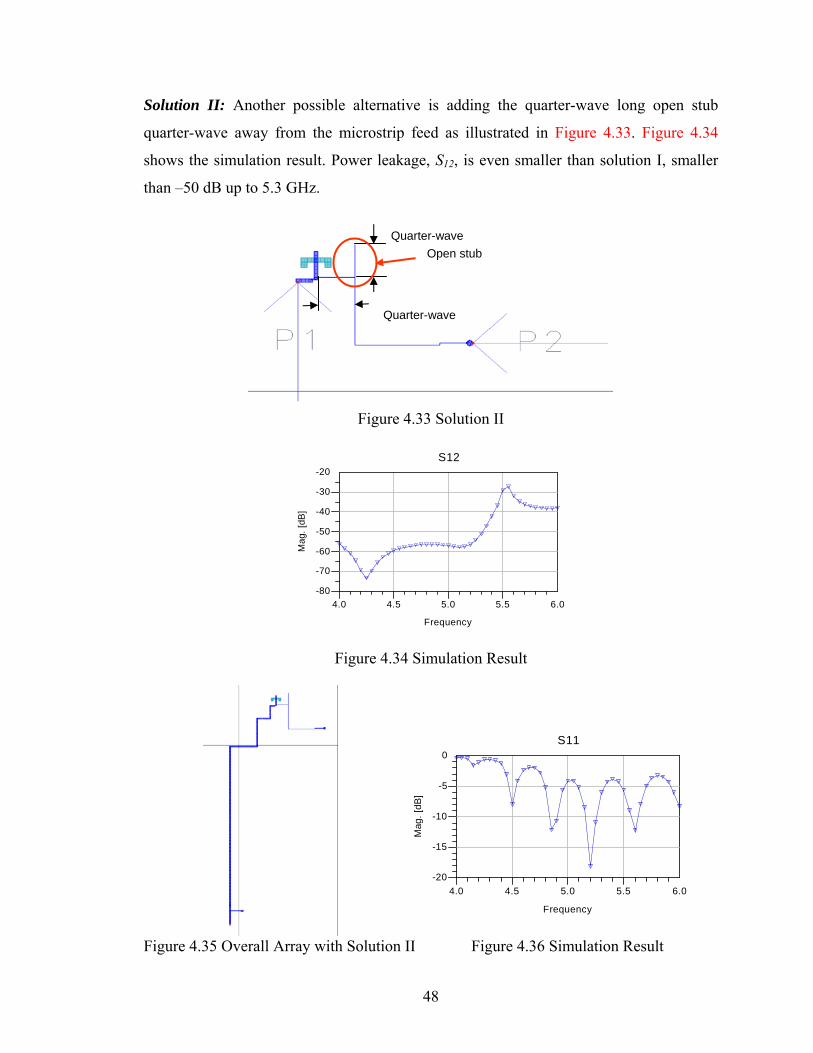
48
Solution II: Another possible alternative is adding the quarter-wave long open stub
quarter-wave away from the microstrip feed as illustrated in Figure 4.33. Figure 4.34
shows the simulation result. Power leakage, S12, is even smaller than solution I, smaller
than –50 dB up to 5.3 GHz.
Figure 4.33 Solution II
4.5 5.0 5.54.0 6.0
-70
-60
-50
-40
-30
-80
-20
Frequency
Mag
. [dB
]
S12
Figure 4.34 Simulation Result
4.5 5.0 5.54.0 6.0
-15
-10
-5
-20
0
Frequency
Mag
. [dB
]
S11
Figure 4.35 Overall Array with Solution II Figure 4.36 Simulation Result
Quarter-wave
Quarter-wave
Open stub

49
Entire array with solution II is simulated to check if the addition of quarter-wave
open stub has any effect on the performance of the antenna. Figure 4.36 proves that this
open stub has no effect: antenna still radiates at 5.2 GHz. This scheme may sound more
attracting than the first solution due to the ease in the fabrication since open stub does not
require drilling holes to create ground.
4.2.2. System Integration
The system integration is in charge of the control module, switching unit to
control network analyzer to generate the measurement data. The white blocks in the
block diagram, as shown in Figure 4.7, will be addressed for the system integration. The
programming details will be showed and the hardware setup will be also described.
Since the antenna array is designed to have 128 bias lines for each transmitting or
receiving end, the key thing is to 1) address antennas by controlling analogue voltage
output sequentially; 2) take the measurement data from network analyzer. The idea of
the first step is that the only one transmitting antenna and one receiving antenna is
activated during each measurement time, which requires only one analogue voltage is
high out of 128 biasing lines for transmit antennas. For the receiving antennas, the same
idea can be applied as the case of transmitting antennas. Then the task is transformed
into controlling the output analogue voltage so that only one is high out of 128. The first
step turned into designing a 1:128 switch given a common analogue input. Figure 4.37
shows the intergrated system with labtop and control module.
(a) Outside View (b) Inside Control Rack
Figure 4.37 Integrated System with Control Rack, Laptop, and Network Analyzer

50
4.2.2.1. Construction of Measurement Matrix
The image reconstruction algorithm needs a measurement matrix to generate a
reconstructed image. The elements of the measurement matrix are scattered fields
measured at receiving antenna, and each of them has the index associated with the
number of transmitting and receiving antenna; the number of row and column of each
element corresponds to the one of transmitting and receiving antenna, respectively.
Since the system has a large number of antennas as transmitting and receiving
elements, the best case to address each antenna sequentially is to have 2 loops with
receiving antennas as the inner loop while transmitting antennas are swept as the outer
loop. In this way, each antenna will be addressed accordingly so that the data will be
constructed as a measurement matrix. As a complete program, initialization of the
system is always required before the measurement is taken. Plus the request of complete
data set is putting the image algorithm right after the measurement is done.
Figure 4.38 Schematic of Algorithm for System Integration

51
4.2.2.2. Component Details
In order to take the measurement data, a computer program is executed in the
computer so that this procedure is going to be done automatically. Since the design of
the antenna is requiring the analogue voltage, external hardware except the computer
would be implemented to provide it. A brief introduction of the software and hardware is
given. The details of each components and protocols are included at Appendix C.
Control Module: The LabView 6i (www.ni.com) was used to control the whole system.
The LabView is a graphical programming language, which provide a nice interface and
many drivers for various instruments are available. In order to measure the signal, it is
needed to control the network analyzer and also to control the analogue voltage for
addressing antenna. This procedure requires a program to be able to control both of them.
Therefore, the LabView is chosen to fulfill this target.
Switching Unit: The LabJack and Texas Instruments Multiplexers were used for
switching unit. LabJack has a number of analogue I/Os as well as digital I/Os, which are
needed in controlling voltage output. It also has a good price to quality ratio and nice
interface. Features used were 1 Analog Output and 25 D-sub I/O connectors, including
16 signal outputs as well as surface mount digital outputs. The maximum frequency of
digital output is 50Hz. Data sheet is available at www.labjack.com.
Figure 4.39 Demo Model of 1:128 Switch
In order to control one output voltage out of 128 lines, the generalized switch
1:128 is needed. The demo model is showed in Figure 4.39. However, no manufacturer
1:128 switch
Analogue Input
Analog selection 1 of 128
High (High)
Low

52
makes it, while 1:8 switch is used frequently. The project team built the 1:128 switch
based on 1:8 switch, and 16 switches were needed. The switch is chosen as Texas
Instruments Multiplexers CD74HC4051E.
Figure 4.40 Texas Instruments Multiplexers CD74HC4051E
The functionality of this analogue multiplexer/switch is that only one output of 8
ones is equal to the common input voltage. By using the enable line, the switch could be
disabled, with the analytic function in Figure 4.41.
Figure 4.41 1:8 Switch
In order to make the 1:128 switch, 16 1:8 switch are used and each enable line are
connected with D-sub 25 connector to LabJack digital outputs. The 16 digital outputs are
programmed so that one of them is low to enable one of 16 chips active; the rest 15
outputs are high, so respectively the 15 chips are disabled. 3 selected address lines are
connected with LabJack surface mount digital outputs. For each combination of 3 digits,
one of 8 outputs is selected to have the same voltage as the common input, for all of
common inputs of 16 chips, they are wired to 5V analogue voltage output of LabJack. In
this way, 1 of 128 switching is realized and the analogue voltage only activate one
antenna element by applying analogue voltage, while the rest are disabled. Figure 4.42
Analogue Input
12345678
A2 A1 A0 EN
Address line and Enable line for 1:8 Switch

53
shows 1:128 switch, the yellow color shows the analog voltage flow: 1 of 16 D sub
digital outputs is low with the rest of outputs maintaining high voltage, resulting only one
chip activated. As the same time, 3 surface mount digital outputs, IO0 IO1 and IO2, are
selecting 1 of 8 outputs of this chip. Therefore, 1 of 128 bias lines has high analog
voltage with the rest having no voltage and one antenna is working due to the bias
voltage applied. Then the 1:128 switch is achieved. 2 sets of switches are used in order
to control both transmit and receive ends.
Figure 4.42 Practical Model of 1:128 Switch
4.2.2.3. Control Program
The LabView program followed the schematic of Figure 4.38 exactly. Starting
with initializing the system, the measurement part is in the middle, then finally ending
with running the image reconstruction algorithm to construct the pictures showing the
concrete conditions.
The network analyzer is initialized at frequency 5.2 GHz, which is the working
frequency of the antenna arrays with the 3 minimal points of measure. Figure 4.43 shows
one of the “frames” in LabView to take the measurement data. There are 4 loops; (1)
1:8 Switch
1:8 Switch
1:8 Switch
1:8 Switch
D-Sub
LabJack
1:8 Selection Surface Mount Digital Outputs
1:16 Selection
Antenna Array
Analogue Output

54
transmit parts outer loop 16 times for chip selection, (2) transmit parts inner loop 8 times
for outputs of single chip, (3) receive parts outer loop 16 times for chip selection, and (4)
receive parts inner loop 8 times for outputs of single chip. Obviously it closely
corresponds to the practical model of 1:128 switch. The content inside the most inner
“frame” shows the procedure of taking the measurement data of S parameter from
network analyzer and save it to file ‘mdata.o’
TX16OUTER
TX8INNER
16
RX8INNER
VISA session dup VISA session
error out_8510c
0
0
Imaginary Corr Data
Real Corr Data
save file path
Number of Points
%.12f
00
00
Mag_dB
20
2 [0..3]
RX16OUTER
1
8
65535
Local ID TX0
set D(i) high Digital I/O Commands TX
15
65535
Digital I/O Data TX
D Conditions TX
error out_TX
0000
IO State WriteIO Direction (In=F, Out=T)
D State WriteD Direction (In=F,Out=T)
IO State ReadD State Read
D Output Latch ReadD Direction Read (In=F,Out=T)
8
1
65535
16
Figure 4.43 Measurement of Data Through Network Analyzer
Figure 4.44 Execution of Imaging Program after Measurement
error out_finala=0
c:\data\nde3d.exe
error out_data

55
As shown in Figure 4.44, the imaging program can be executed right after the
previous loops are done. The LabView program is calling a command window of the
operating system, so that an executable file could be run through LabView program. The
imaging program ‘nde3d.exe’ is called in the most upper pink window.
Figure 4.45 shows the panel interface of the program. Basically the diagram does
not have to be understood in order to run the program. The panel interface provides the
controllers and indicators. Controllers are those items that could be changed by user.
Usually the parameters in the controller parts do not need to be modified. The default
value is what’s going to be needed during the measurement. For example, for the
scattered field measurement, the default value is S21, which supposes the transmit
antennas are connected with port 1 of network analyzer, while the receive antennas are
connected with port 2. If the positions of transmit and receive antennas exchange, S12
may be obtained from the S parameter controller.
Figure 4.45 Panel Interface

56
Indicators show the status of the system. There are 2 sets of commands and status
of the I/O digital outputs, through the 2 most left columns. The light gray column in the
middle tells you the ID number of the LabJacks currently used for transmit and receive
ends. As the lower part, the S parameter reading is showed simultaneously, the numbers
are changing during the measurement. The magnitude of it is shown also. Error
indicators are showing if there are abnormal things happening. If there are, the error
information is given. In the normal measurement procedure, errors are not likely to be
happened, so just check and make sure the controllers are having the right settings.
4.2.2.4. Measurement Speed Evaluation
In order to evaluate how fast the measurement is done, the 1st and 2nd outputs of
the switching units were connected to oscilloscope to record the required time. Figure
4.46 shows that one time measurement takes about 40ms, which means totally the
measurement takes about 15 minutes.
Figure 4.46 Measurement Time Shown in Oscilloscope
0.4 20.4 40.4 60.4 80.4 100 120 140 160 180-1
0
1
2
3
4
5
6
~40ms
V
Time (ms)

57
Chapter 5
NUMERICAL SIMULATION
Numerical simulations were carried out to test the proposed algorithm for the
image reconstruction of a concrete specimen with internal air voids and steel bars. The
reconstruction parameters including effective focusing area were investigated. Totally 7
cases were modeled with 5.2GHz as an illuminating frequency and the image of each
case was reconstructed. Some of these numerical simulations were compared with the
results with 10.0GHz as the illuminating frequency. This comparison showed that the
resolution can be improved by using the higher illuminating frequency. For the
simulation, planar rectangular antenna arrays were used with 8 transmitting/receiving
antennas for the case of 5.2GHz and 16 transmitting/receiving antennas for the case of
10.0GHz. For simplicity, only a 2D rectangular geometry was considered for the
investigation and only Y polarization of the antenna was used. Extension to 3D can be
easily obtained by using the spherical Green’s function as a focusing operator instead of
the Hankel function.
5.1. Effective Focusing Area (EFA)
Reconstruction parameters such as focusing intensity and impulse response of the
system for the planar antenna array were investigated. Based on the results of a
parametric study using point-like objects, the effective focusing area (EFA), in which the
focusing operation is effective, was determined. In other words, the focusing intensity
level and impulse response shape has a good uniformity in the effective focusing area.
Also, the effective penetration depth is determined by the effective focusing area. The
shape and size of the effective focusing area (penetration depth) strongly depend not only
on the electrical size of the measuring line, but also on the arrangement of the
transmitting and receiving elements, which means that the EFA of a planar antenna array
differs from the one for circular antenna array. Through a series of simulation using

58
point-like objects, in which the focusing intensity level and shape of impulse response at
different locations were compared, the effective focusing area was determined as the
shape of a trapezoid, as represented in Figure 5.1.
x
y
Effective Focusing Area
Array
0.2
m
0.1 m
0.0125 m0.0625 m
0.07
5 m
0.12
5 m
Figure 5.1 Effective focusing area of planar rectangular antenna array
5.2. Simulation Results Using 5.2 GHz
Based on the reconstruction parameters, especially the effective focusing area,
numerical simulations were carried out. For the direct problem in which the antenna
radiates a wave and receives the scattered field, a 3D structure simulator, CST
Microwave Studio®, was used for measuring the transmission parameters (Sij) in each
array. Totally, seven geometries were modeled with a 16-slot antenna. In the simulation,
the background material was modeled as concrete so as to radiate the wave through the
concrete. Open boundary conditions were applied at the top and the bottom of the
geometry in order to generate absorbing conditions.

59
Using the Sij measurements from each array, the measurement matrix of Eqn.
(3.12) was assembled and the electromagnetic image of Ef(rf) at rf=(xf , yf) was obtained
as presented previously.
All the objects used in the numerical simulation were located inside of the
effective focusing area. The reconstructed images for each case are reported in Figure 5.2
along with the model description and the reconstructed area.
In case 1, the air sphere was successfully reconstructed with exact location and
size as represented in Figure 5.2(a). The reconstructed area was limited to 5cm in x-
direction because the open boundary in CST Microwave StudioTM was set at the y-axis,
from which the distance to the antenna array is 5cm. The reconstructed area in the x-
direction for the other cases was also determined by the location of an open boundary
(10cm in the x-direction).
In cases 2 and 3, a square and a rectangular air block were placed inside the
concrete material, respectively. As shown in Figure 5.2(e) and (f), the reconstructed
image shows the exact location and the approximate size of the air blocks in both cases,
although there was some noise. These two cases were investigated again at the higher
frequency in order to demonstrate the improvement of resolution.
Cases 4 and 5 show the transverse and longitudinal resolution of the system,
respectively. The wavelength in concrete at 5.2GHz is about 2.5cm, which provides the
resolution of the system of 2.5cm. As represented in Figure 5.2(b), the locations of two
steel bars separated with transverse distance of 2.5cm (λe) were detected apparently,
although the resolution was not sufficient enough to reconstruct the exact shapes of the
bars. Figure 5.2(c) shows the reconstructed image of two steel bars placed at a
longitudinal distance of 2.5cm (λe). In this case, the two bars could be successfully
identified, but the exact shapes could not be reconstructed due to the lack of resolution.
From the results of cases 2 and 3, it was demonstrated that the resolution of the system
with planar antenna array is of the order of a wavelength in concrete (2.5cm), which can
identify the approximate shapes and locations.
In case 6, six steel bars were placed at the boundaries of the effective focusing
area for the reconstructing of a 2D cross section. The result, as shown in Figure 5.2(d),
demonstrated that the objects near the antenna arrays are more clearly identified rather

60
than the ones at the farther boundaries of effective focusing area, which is marked by
black line, from the antenna array.
In case 7, a steel square bar and an air block were placed inside the concrete
material. The difference in the dielectric constant between steel and concrete is much
bigger than the one between air and concrete. For this reason the air void is more difficult
to detect than the steel bar. As shown in Figure 5.2(g), although the steel is located far
from the antenna array, the main features are correctly located, including size and
position, while for the air void only the location is detected.
Using the results of the numerical simulation, the efficiency of the image
reconstruction algorithm was tested through different cases, including steel, air voids, or
combinations of the above. Within the effective focusing area, the location and size of
objects were successfully detected.
x
Steel Sphere(r = 0.01m)
Reconstructed Area
Antenna Array
Concrete Panel
0.04 m
0.2
m
0.00 0.02 0.04
x (m)
-0.10
-0.08
-0.06
-0.04
-0.02
-0.00
0.02
0.04
0.06
0.08
0.10
y (m
)
(a) Case 1
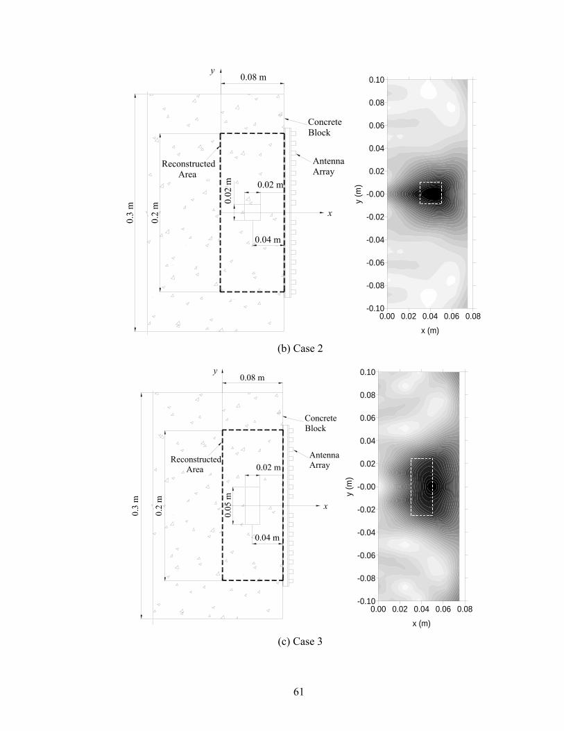
61
x
Reconstructed Area
Antenna Array
Concrete Block
0.08 m
0.3
m
0.2
m
0.02 m
0.02
m0.04 m
0.00 0.02 0.04 0.06 0.08
x (m)
-0.10
-0.08
-0.06
-0.04
-0.02
-0.00
0.02
0.04
0.06
0.08
0.10
y (m
)
(b) Case 2
x
y
Reconstructed Area
Antenna Array
Concrete Block
0.08 m
0.2
m
0.3
m
0.02 m
0.04 m
0.05
m
0.00 0.02 0.04 0.06 0.08
x (m)
-0.10
-0.08
-0.06
-0.04
-0.02
-0.00
0.02
0.04
0.06
0.08
0.10
y (m
)
(c) Case 3

62
x
Reconstructed Area Array
0.1 m
0.2
m
0.05 m
0.02
5 m 5 mm
0.00 0.02 0.04 0.06 0.08 0.10
x (m)
-0.10
-0.08
-0.06
-0.04
-0.02
-0.00
0.02
0.04
0.06
0.08
0.10
y (m
)
(d) Case 4
x
Reconstructed Area Antenna
Array
0.1 m
0.2
m
0.05 m
0.025 m
5 mm
0.00 0.02 0.04 0.06 0.08 0.10
x (m)
-0.10
-0.08
-0.06
-0.04
-0.02
-0.00
0.02
0.04
0.06
0.08
0.10
y (m
)
(e) Case 5

63
x
Reconstructed Area
Antenna Array
0.2
m
0.0625 m 0.0125 m
0.12
5 m
0.07
5 m
0.00 0.02 0.04 0.06 0.08 0.10
x (m)
-0.10
-0.08
-0.06
-0.04
-0.02
-0.00
0.02
0.04
0.06
0.08
0.10
y (m
)
(f) Case 6
x
y
Reconstructed Area
Antenna Array
0.2
m
0.1 m
0.01 m
0.05
m
0.06
m
0.035 m
0.01
cm
0.06 m
0.01 m
EFA
0.00 0.02 0.04 0.06 0.08 0.10
x (m)
-0.10
-0.08
-0.06
-0.04
-0.02
-0.00
0.02
0.04
0.06
0.08
0.10
y (m
)
(g) Case 7
Figure 5.2 Simulation Results with Descriptions

64
5.3. Simulation Results Using 10.0 GHz
In the antenna design, the illuminating frequency was determined as 5.2GHz as a
good compromise between a set of different parameters, such as size, resolution,
attenuation, and simplicity of prototype. For that reason, the resolution of the system, as
shown in the previous simulation results, was limited to 2.5cm and the exact shape of the
object inside concrete could not be reconstructed. Better resolution, however, can be
obtained by increasing the illuminating frequency.
In order to demonstrate the improvement of resolution using higher illuminating
frequency, cases 5 and case 6 were investigated again with 10.0GHz as an illuminating
frequency. For the numerical simulation, the planar rectangular antenna arrays with 16
transmitting and 16 receiving antennas were used. The results in Figure 5.3 show that the
resolution of the reconstructed image can be improved by increasing the illuminating
frequency and that the exact shape and location of the voids can be reconstructed when
using 10.0GHz.
0.00 0.02 0.04 0.06 0.08
x (m)
-0.10
-0.08
-0.06
-0.04
-0.02
-0.00
0.02
0.04
0.06
0.08
0.10
y (m
)
0.00 0.02 0.04 0.06 0.08
x (m)
-0.10
-0.08
-0.06
-0.04
-0.02
-0.00
0.02
0.04
0.06
0.08
0.10
y (m
)
(a) Case 5 using 5.2GHz (b) Case 5 using 10.0GHz

65
0.00 0.02 0.04 0.06 0.08
x (m)
-0.10
-0.08
-0.06
-0.04
-0.02
-0.00
0.02
0.04
0.06
0.08
0.10
y (m
)
0.00 0.02 0.04 0.06 0.08
x (m)
-0.10
-0.08
-0.06
-0.04
-0.02
-0.00
0.02
0.04
0.06
0.08
0.10
y (m
)
(c) Case 6 using 5.2GHz (d) Case 6 using 10.0GHz
Figure 5.3 Resolution Improvement Using Higher Frequency

66
Chapter 6
EXPERIMENTAL VERIFICATION
6.1. Microwave Imaging Using Prototype I
In this section, the effectiveness of the proposed sub-surface imaging technology
using the prototype I system was investigated through a series of experiments on a
concrete panel and a concrete block.
6.1.1 Experimental Setup
The effectiveness of the proposed sub-surface imaging technology was further
investigated through a series of experiments on a concrete panel and a concrete block. A
steel rod was placed on one of the faces of the concrete panel to simulate steel rebar. The
30 cm × 30 cm × 30 cm concrete block involves two internal voids artificially generated
using Styrofoam (whose dielectric property is the same as that of the air); one is a 2 cm
cubic void and the other is a 5 cm × 2 cm × 2 cm void. The Styrofoam blocks were
inserted into the concrete during the pouring of concrete with the distance of 3 cm from
the face of concrete to the face of Styrofoam in both cases. Samples using steel bars in
the air were also prepared. All the experimental cases, identical to those used in the
numerical simulation, were described in Table 6.1.
Table 6.1 Descriptions of Cases for Experimental Study
Case number Description
Reconstructed Area (x × y)
(cm×cm)
Exact Locations of Objects (x,y) (cm)
1 Steel sphere at the center of concrete panel 4 × 20 (0,0)
2 square air void inside concrete 8 × 20 (4,0)
3 rectangular air void inside concrete 8 × 20 (4,0)

67
The experimental setup consisted of a network analyzer, a switch box, coaxial
cables and the antenna array as shown in Figure 6.1. The network analyzer is a two-port
device capable of transmitting a signal at one port and receiving a signal at the other port
while evaluating the magnitude and phase of the receiving signal. The network analyzer
was used to evaluate the signal transmitted through the medium (S12). The switch box
developed in this study is a radio frequency network capable of controlling multiple
antennas in the array and selecting them individually to perform S12 measurement.
Figure 6.1 Experimental Setup
Calibration was performed to remove the effect of wave reflections and loss in the
coaxial cables and the switch box from the measured signals (Kim 2002, Kim et al.,
2002). For the calibration purpose, concrete panel without defect and steel plate are used
as represented in Figure 6.2.
Each transmission measurement without all the effects from the coaxial cables
and the switch box, which is from the transmitting array to the receiving one, is
proportional to the zero-order Hankel function of the second kind, H0(2)(ke,concdij), whose
argument is proportional to the distance from the transmitting array to the receiving one,
dij (Balanis, 1998). All the measurement effects from the coaxial cables and the switch
box (calibration factor), therefore, can be calculated by dividing each transmission
measurement of calibration (Sij(cal_mea)) by the zero-order Hankel function of the second
kind, and the calibrated transmission measurement (Sij(cal)) can be obtained by dividing
Network Analyzer
Power Supply
Switch Box
Antenna Array
Concrete Block

68
each transmission measurement (Sij(mea)) by calibration factor, as follows for the case of
transmitting array i and receiving array j.
( )
( )
_
meacal ij
ij
SS
Cal Factor= (6.1)
where
( _ )
(2)0 ,
_( )
cal meaij
e conc ij
SCal factor
H k d= (6.2)
Amplitudes of calibrated measurements in a concrete without defects are
proportional to the distance between the transmitting and the receiving arrays, and
symmetric with respect to the diagonal in a measurement matrix. The calibration factors
of each transmission measurement at 5.2 GHz are used for calculating the calibrated
measurement matrix in next section.
1 2 3 4 5 6 7 8 9 10 11 12 13 14 15 16
Transmitting Array Receiving Array
d1,9
Steel Plate
d1,16
d8,10
d8,16
Concrete Panel
Figure 6.2 Description of Calibration Scheme
6.1.2 Experimental Results
A continuous 5.2 GHz sinusoidal electromagnetic (EM) wave was generated from
the signal analyzer and sent to the test specimen. Transmission measurements of each
transmitting and receiving array pair at this frequency were assembled to form a
measurement matrix. The switch box controlled the active location of the transmitting
and receiving arrays from S1,9 to S8,16. Each measured signal was divided by the
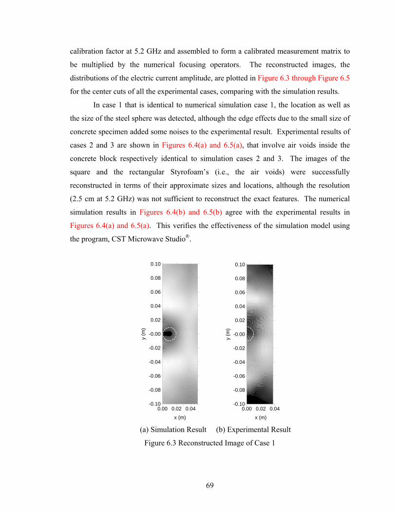
69
calibration factor at 5.2 GHz and assembled to form a calibrated measurement matrix to
be multiplied by the numerical focusing operators. The reconstructed images, the
distributions of the electric current amplitude, are plotted in Figure 6.3 through Figure 6.5
for the center cuts of all the experimental cases, comparing with the simulation results.
In case 1 that is identical to numerical simulation case 1, the location as well as
the size of the steel sphere was detected, although the edge effects due to the small size of
concrete specimen added some noises to the experimental result. Experimental results of
cases 2 and 3 are shown in Figures 6.4(a) and 6.5(a), that involve air voids inside the
concrete block respectively identical to simulation cases 2 and 3. The images of the
square and the rectangular Styrofoam’s (i.e., the air voids) were successfully
reconstructed in terms of their approximate sizes and locations, although the resolution
(2.5 cm at 5.2 GHz) was not sufficient to reconstruct the exact features. The numerical
simulation results in Figures 6.4(b) and 6.5(b) agree with the experimental results in
Figures 6.4(a) and 6.5(a). This verifies the effectiveness of the simulation model using
the program, CST Microwave Studio®.
0.00 0.02 0.04
x (m)
-0.10
-0.08
-0.06
-0.04
-0.02
-0.00
0.02
0.04
0.06
0.08
0.10
y (m
)
0.00 0.02 0.04
x (m)
-0.10
-0.08
-0.06
-0.04
-0.02
-0.00
0.02
0.04
0.06
0.08
0.10
y (m
)
(a) Simulation Result (b) Experimental Result
Figure 6.3 Reconstructed Image of Case 1

70
0.00 0.02 0.04 0.06 0.08
x (m)
-0.10
-0.08
-0.06
-0.04
-0.02
-0.00
0.02
0.04
0.06
0.08
0.10
y (m
)
0.00 0.02 0.04 0.06 0.08
x (m)
-0.10
-0.08
-0.06
-0.04
-0.02
-0.00
0.02
0.04
0.06
0.08
0.10
y (m
)
(a) Simulation Result (b) Experimental Result
Figure 6.4 Reconstructed Image of Case 2
0.00 0.02 0.04 0.06 0.08
x (m)
-0.10
-0.08
-0.06
-0.04
-0.02
-0.00
0.02
0.04
0.06
0.08
0.10
y (m
)
0.00 0.02 0.04 0.06 0.08
x (m)
-0.10
-0.08
-0.06
-0.04
-0.02
-0.00
0.02
0.04
0.06
0.08
0.10
y (m
)
(a) Simulation Result (b) Experimental Result
Figure 6.5 Reconstructed Image of Case 3

71
Chapter 7
OPERATOR’S MANUAL OF IMAGING SYSTEM
This document is an operator’s manual of the imaging system explaining the
usage of the system and the communication details between the modules and function of
each unit.
System Description
This microwave image reconstruction system is for condition assessment of
concrete structures. The system consists of several units including a control module, a
switching unit, an antenna array, a network analyzer, an image reconstruction algorithm,
and a display unit. The final product to the user is a reconstructed image of the object
under testing, showing 3-dimensional profiles of the object. The reconstructed image is
generated using the scattered field by microwave illumination using the antenna array.
The measurement is performed by electronically switching the antenna array controlled
by the control module and software. The following Figures 7.1 and 2 describe the job
flow and the block diagram of the system, and Figure 7.3 shows a picture of the system.
Figure 7.1 Job Flow of the System

72
Figure 7.2 Block Diagram of the System
Figure 7.3 Outside View of the System
Network Analyzer
Control Module
Main Computer (Control Software, Imaging Software,
Visualization)

73
How to Operate the System?
The operation of the system consists of three steps: initialization, measurement,
and visualization. At each step, the following operations are needed.
1. Initialization
When the operator runs the program named ‘caltrans.exe’, the first step of
initialization is to determine and enter the system parameters:
- Frequency (5.2GHz): illuminating frequency
- Analogue Voltage Output (5V): voltage output to control switches
- S-parameter (S21): measurement from the network analyzer
- Save File Path (“mdata.o”): measurement matrix file name and path. File
name should always be “mdata.o”.
If the system is operating under the normal condition, the operator can use default
values of 5.2, 5.00, S21, and “mdata.o”. Figure A.4 shows the front panel
displayed in the labtop including the system parameter input part.
(a) Front Panel View

74
(b) System Parameter Input (default values)
Figure 7.4 Front Panel of Control Module
2. Measurement
Once the system parameters are set, the operator can put the antenna array on the
object to be investigated and click the “RUN” button at the top of the front panel.
The control module program will automatically transmit and receive the
microwave signal through the antenna array by switching each antenna elements.
3. Visualization
At the end of the measurement, the control module program will automatically
execute the image reconstruction program named as ‘nde3d.exe’ opening a new
window. The image reconstruction program analyzes the measurement matrix
and displays cut images at several vertical locations in the reconstructed volume,
and then the operator can select and magnify any of the cut images to investigate
in details. Details of the image reconstruction program are introduced at
Appendix B.
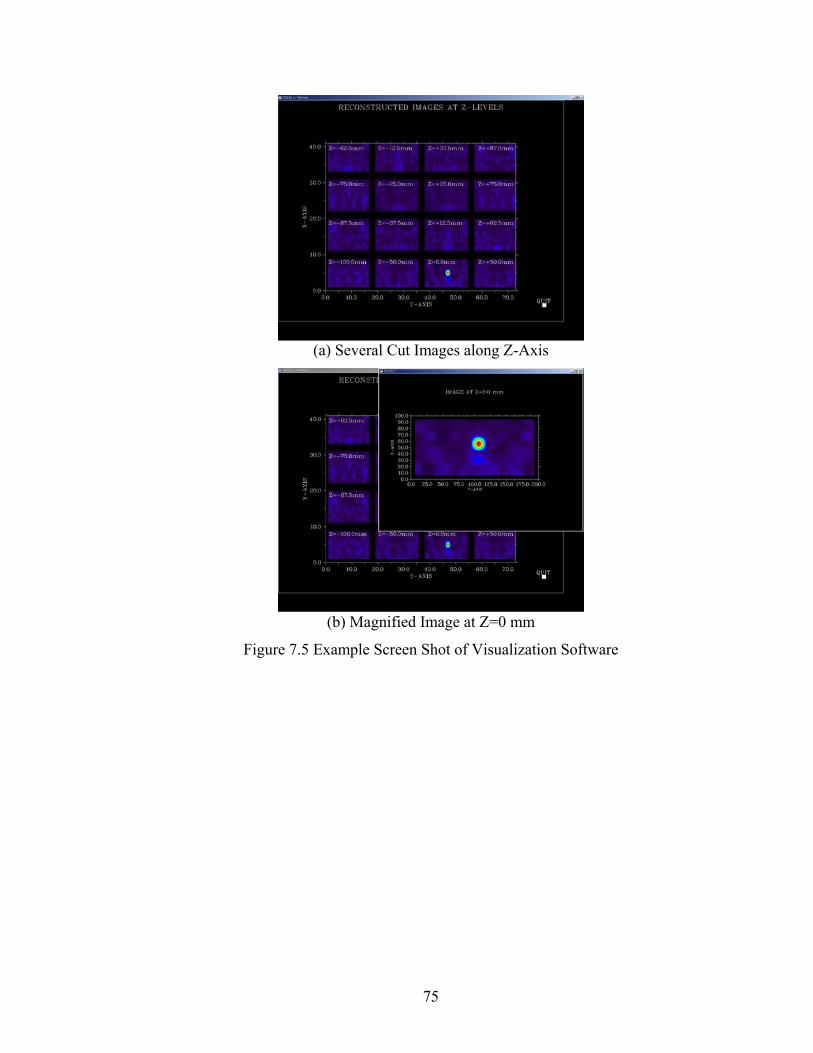
75
(a) Several Cut Images along Z-Axis
(b) Magnified Image at Z=0 mm
Figure 7.5 Example Screen Shot of Visualization Software

76
Chapter 8
SUMMARY AND CONCLUDING REMARKS
A sub-surface focused microwave imaging technology was developed in this
project for detecting invisible damage and/or objects inside concrete structures.
Significant theoretical, analytical, numerical, and experimental studies have been carried
out in this project, laying a theoretical and technical foundation for the implementation of
the microwave imaging technology. This project has delivered two prototype microwave
imaging systems including hardware (antenna arrays involving a large number of
antennas, switching and control circuitry) and software (imaging reconstruction and
visualization). One of the systems was successfully tested through experiments on
concrete specimen. The following concluding remarks can be made:
(1) The effectiveness of the image reconstruction algorithm using the innovative
numerical bi-focusing operator proposed in this study was verified experimentally
as well as numerically. An image resolution in the order of the wavelength in a
dielectric medium (concrete in this case) can be achieved by focusing both in the
transmitting and receiving arrays, which doubles the resolution achievable by the
conventional mono-focusing
(2) The multi-frequency technique proposed in this project is effective in reducing the
background noise and thus enhancing the clarity of the reconstructed image.
(3) Experiments verified that the slot type of the antenna array is suitable for damage
detection of concrete structures due to its high radiation performance and
bandwidth as well as low mutual coupling among the antennas.
(4) Prototype I successfully detected size and depth of invisible air voids and steel
inside concrete specimens.
(5) Prototype II successfully integrated four major modules including the antenna
arrays, the control module, software in PC, and a network analyzer into a portable
system. The control module under the control of the software effectively controls
the bias for diodes to switch antenna with a high speed.

77
Nomenclature
Ei Incident Electric Field
Es Scattered Electric Field
J Electric current distribution
Jeq Equivalent electric current distribution
Sii Scattering parameter (reflection parameter)
Sij Scattering parameter (transmission parameter)
k0 Wave number in air
ke Effective wave number in a medium
εr Relative dielectric constant
λ0 Wave Length in air
λe Effective wave length in a medium

78
References
Balanis, Constantine A. (1989), Advanced Engineering Electromagnetics, Wiley, New
York.
Broquetas, A., Romeu, J., Rius, J.M., Elias-Fuste, A., Cardama, A., Jofre, L. (1991),
“Cylindrical Geometry: A Further Step in Active Microwave Tomography”, IEEE
Trans. on Microwave Theory and Techniques, 39, 836-844, May.
Bucci, O. M., Crocco, L., Isernia, T., and Pascazio, V. (2000), “Inverse Scattering
Problems with Multifrequency Data; Reconstruction Capabilities and Solution
Strategies”, IEEE Trans. Geoscience and Remote sensing, 38(4), 1749-1756.
Chase, S. B. and Washer, G. (1997), “Nondestructive Evaluation of Bridge Management
in the Next Century”, Public Roads, July/August, 16-24
CST-Computer Simulation Technology (2002), HF Design and Analysis – CST
Microwave Studio® 4, Software Manual.
Dunker, K.F.and Rabbat, B.G. (1990), “Highway Bridge Type and Performance Patterns”,
Journal of Performance of Constructed Facilities, ASCE, 4(3), 161-173.
Feng, M. Q., Flaviis, F. D., and Kim, Y. J. (2002), “Use of Microwaves for Damage
Detection of Fiber Reinforced Polymer-Wrapped Concrete Structures”, Journal of
Engineering Mechanics, ASCE, 128(2), 172-183.
FHWA, (1998), “Transportation Equity Active for 21 Century (TEA-21)”,
http://www.fhwa.dot.gov/tea21/factsheet/bridge.htm
Garg, R., Bhartia, P., Bahl, I., and Ittipiboon, A. (2001), Microstrip Antenna Design
Handbook, Artech House, Boston.
Gironés, I.M., Jofre, L, Ferrando, M., De Los Reyes, M, and Bolomey, J. Ch. (1987),
“Microwave Imaging with Crossed Linear Arrays”, IEE Proceedings, 134(3),
June, 249-252.
Harrington, R. F. (1961), Time Harmonic Electromagnetic Fields, McGraw Hill, New
York
Haroun, M. A. and Feng, M.Q. (1997), “Lap Splice and Shear Enhancements in
Composite-Jacketed Bridge Columns”, Proceedings of the 3rd US-Japan Bridge
Workshop, Tsububa, Japan

79
Kim, Y. J. (2002), Development of Electromagnetic Imaging Technology for Damage
Detection, Ph.D. Dissertation, University of California, Irvine, CA.
Kim, Y. J., Jofre, L., De Flaviis, F., and Feng, M. Q. (2002), “Microwave Sub-Surface
Imaging Technology for Damage Detection of Concrete Structures”, Proceedings
of 15th ASCE Engineering Mechanics Division Conference, New York, June, 589-
596.
Mast, J., Azevedo, S., Hadda, W., Ng, L., and Burnett, G. (1998), “Microwave Impulse
Radar Technology and Applications”, Report of Lawrence Livermore National
Laboratory, UCRL-ID-130474
Olson, L. D., Jalinoos, F., Aouad, M. F., and Balch, A. H. (1993), “Acoustic tomography
and reflection imaging for nondestructive evaluation of structural concrete”, NSF
SBIR Final Report (Award #9260840), Washington, D.C.
Pierri, R., Brancaccio, A., and De Blasio, F. (2000), “Multifrequency Dielectric Profile
Inversion for a Cylindrically Stratified Medium”, IEEE Trans. Geoscience and
Remote sensing, 38(4), 1716-1724.
Slaney, M., Kak, A. C., and Larsen, L. E. (1984), “Limitations of Imaging with First-
Order Diffraction Tomography”, IEEE Trans. Microwave Theory and Techniques,
MTT-32(8), 860-874.
Weil, G. (1994), “Nondestructive Testing of Bridge, Highway, and Airport Pavements”,
Journal of Applied Geophysics, August

80
Appendix A
REFERENCE MANUAL OF MUDULES
Communications Between the Modules
1. Control Module – Switching Unit (LabJack)
Control module (LabView) sends signals to switching unit of LabJack in order to
control the switches in the antenna array. Since the Labjack has the LabView VIs,
LabView program needs to have the following functions (also shown in Figure A.1):
1) Give out the output signal of control antenna array
i. Transmit antenna switching on one by one
ii. Receive antenna switching on one by one when one transmit
antenna is switched on
2) Control signal of the network analyzer
3) Give a certain time to collect the S parameter measurement data (read data
from network analyzer). In total there are 128×128 times reading and
saving.
Here the measurement speed is dependant on the network analyzer, how fast it
could be able to obtain the S parameter data.

81
Select transmitting antenna byanalog output of the Labjack andmultiple 1:16 switches
Select receiving antenna byanalog output of the Labjack andmultiple 1:16 switches
Give out a control signal throughthe Labjack to take the S-parameters
Read the S-parameter throughthe Labjack and save it
Inner loop 128 times
Outer loop 128 times Figure A.1 Schematic of Algorithm

82
2. Switching Unit (LabJack) – Antenna Array
Analog output of switching unit (labjack) will be connected with 1:16 switch to
control the antenna array, Figure A.7 shows the sample of a 16 antenna array, and Figure
A.8 shows the truth table in which we know how to select only one of the 16th output to
make it high to activate the antenna. For our case, by utilizing the enable line, we could
expand to control 2 sets of 128-antenna array. The voltage need to switch “on ” is greater
than 2.4v according to the data sheet of this 1:16 switch.
The labjack needs to control the transmit antenna and receive antenna array. The
Figure A.2 shows how the control signal goes.
Figure A.2 Practical Model of 1:128 Switch
labjack
analong ouput
1:16switch . . . 1:16switch
. . .
. . .
analong selection 1 of 128
1:16switch . . . 1:16switch
. . .
. . .
Transmit antenna Control, 8 sets
Receive antenna Control, 8 sets

83
3. Antenna Array – Network Analyzer
In our case the network analyzer takes the S parameter data once the transmitting and
receiving antenna is switched on. To read the data from network analyzer and store the
data according to its corresponding antenna is realized by LabView programs.
The following graph shows how to get the measurement data:
Figure A.3 Communication Between LabJack and Network Analyzer
Labjack analog input
Network analyzer
analong selection 1 of 128
analog selection 1 of 128 rx
tx

84
4. Network Analyzer – Image Reconstruction Algorithm
The image reconstruction algorithm needs a measurement matrix to generate a
reconstructed image. The elements of the measurement matrix are scattered fields
measured at receiving antenna, and each of them has the index associated with the
number of transmitting and receiving antenna; the number of row and column of each
element corresponds to the one of transmitting and receiving antenna, respectively.
Figure A.4 describes the numbering of antenna element and corresponding location of the
scattered field in the measurement matrix.
Measurement matrix:
, 1 1 , 1 2 , 1 128
, 2 1 , 2 2 , 2 128
, 128 1 , 128 2 , 128 128
s T R s T R s T R
s T R s T R s T R
s T R s T R s T R
E E E
E E E
E E E
⎡ ⎤⎢ ⎥⎢ ⎥⎢ ⎥⎢ ⎥⎣ ⎦
L
L
M M O M
L
Figure A.4 Element of Measurement Matrix Corresponding to the Number of Element in Antenna Array
The algorithm needs a file as an input, which has scattered field in complex
number) in a matrix form, in ASCII format as follows.
ES,T1,R1(complex) ES,T1,R2 ES,T1,R3 ES,T1,R4 …
ES,T2,R1 ES,T2,R2 …
…
ES,T128,R128 …
TransmittingArray
ReceivingArray
1
2
3
4
5
6
7
8
9
10
11
496581978197 65 49 1
2
3
4
5
6
7
8
9
10
11
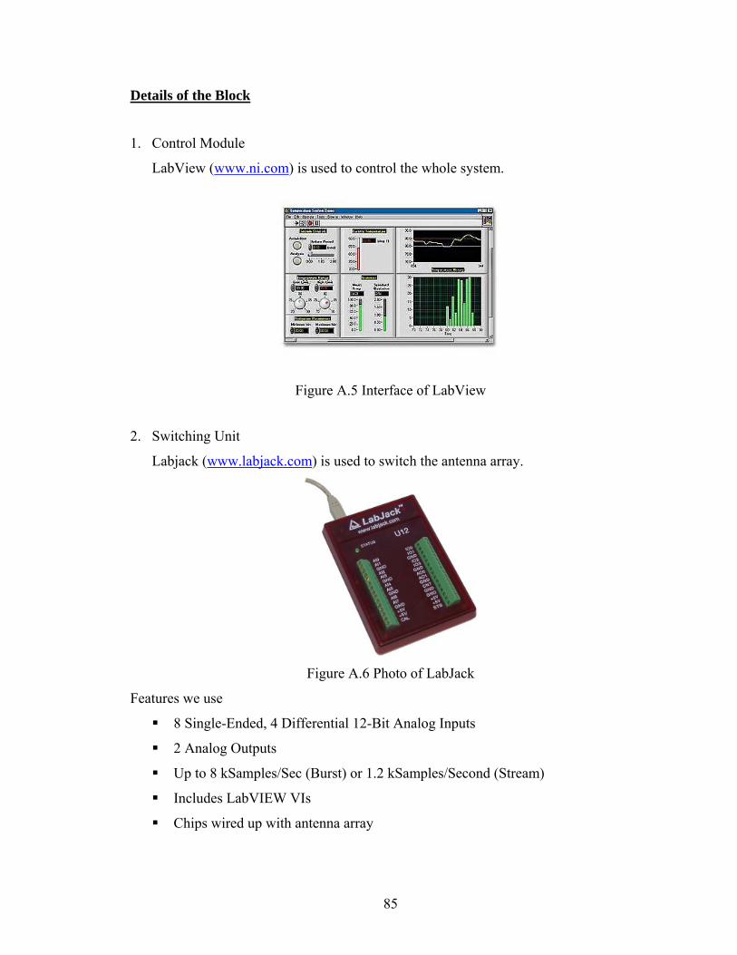
85
Details of the Block
1. Control Module
LabView (www.ni.com) is used to control the whole system.
Figure A.5 Interface of LabView
2. Switching Unit
Labjack (www.labjack.com) is used to switch the antenna array.
Figure A.6 Photo of LabJack
Features we use
8 Single-Ended, 4 Differential 12-Bit Analog Inputs
2 Analog Outputs
Up to 8 kSamples/Sec (Burst) or 1.2 kSamples/Second (Stream)
Includes LabVIEW VIs
Chips wired up with antenna array

86
Figure A.7 Using the LabJack with Enable Line and Address Line
Figure A.8 Truth table of MAX396
analog inputfrom labjack
antenna array1*16 example
output
123456789
10111213141516
1: 16 switch
A3 A2 A1 A0 ENaddress line andenable line for
MAX396

87
Appendix B
MANUAL OF IMAGE RECONSTRUCTION PROGRAM
Description
The program NDE3D is an image reconstruction program using measurement
data file, ‘mdata.o’, which is saved as an ASCII file from network analyzer. NDE3D is
embedded on the Labview program, set to be run after the measurement and saving it as
an ASCII file.
The measurement data is saved as a matrix format (128 by 128). NDE3D loads
the file, multiply the matrix with a focusing operator, which will be explained in next
section, and show the cut images along the Z-axis in a window. Each image is an XY
plane cut at 16 different locations along Z-axis. The user can pick one of the images to
magnify in another window and to investigate more detail. The graphic library used in
NDE3D is DISLIN 8.0B, which is developed by Helmut Michels in Germany.
Theory
Formulation of the image reconstruction algorithm was introduced in Chapter 3 of
the report.
Input File
NDE3D needs two input files of measurement data and transformation
information. Measurement data is an ASCII format file containing 128 by 128 matrix, in
which each element is an amplitude of scattered field measured at each receiving antenna.
The name of the file is ‘mdata.o’.
The transformation information is also needed because the number of each
antenna element differs from the one in control system. The file contains two numbers in
a row, the number in control system and the corresponding number of real antenna
element. The name of the file is ‘trans.in’.

88
Code List with Comments
C******************************************************************** PROGRAM MAIN C******************************************************************** USE DISLIN CHARACTER*16 MEASURE,TRANSFORM COMPLEX J COMPLEX FO_RMN,FO_TKL,TMP1,TMP2 COMPLEX SE_F(16,8,17),E_F(16,8,17),MEA(128,128),MEA_T(128,128), 1 MEA_TR(128,128) COMPLEX IT(128),IR(128) REAL FREQ(10),KE(10) C COMMON /IOUNIT/IIN,IOUT COMMON XT,YT,ZT,XR,YR,ZR COMMON XF,YF,ZF C DIMENSION XT(16),YT(16),ZT(8),XR(16),YR(16),ZR(8) DIMENSION XF(8),YF(16),ZF(17) DIMENSION XO(100),YO(100),ZO(100),OBJ(100) DIMENSION ABS_SE_F(16,8,17) DIMENSION NTRM(128) DIMENSION TTT(256) DIMENSION NSLICE(17) C PARAMETER (NXRAY=73, NYRAY=41) DIMENSION RE(73,41), RE_S(16,8) C DIMENSION XRAY(73),YRAY(41),ZLEV(350),XRAY_S(16),YRAY_S(8) C IME=7 ITR=8 C PI=3.14159265358979 J=(0.,1.) C CALL OPENFILE C******************************************************************** C GENERATE TX&RX LOCATION C******************************************************************** DX=0. DY=12.5 DZ=12.5 C DO K=1,16 XT(K)=100. XR(K)=100. ENDDO C DO K=1,8 ZT(K)=100.-DZ*(K-1) ZR(K)=-12.5-DZ*(K-1) ENDDO C DO L=1,16 YT(L)=6.25+DY*(L-1) YR(L)=6.25+DY*(L-1) ENDDO C******************************************************************** C GENERATE RECONSTRUCTION VOLUME C******************************************************************** DX=12.5 DY=12.5 DZ=12.5 C DO K=1,8 XF(K)=6.25+DX*(K-1) ENDDO DO L=1,16 YF(L)=6.25+DY*(L-1) ENDDO DO M=1,17 ZF(M)=-100+DZ*(M-1) ENDDO C******************************************************************** C READ FREQUENCY INFORMATION C******************************************************************** N_FREQ=1

89
C READ(IIN,*) (FREQ(N),N=1,N_FREQ) FREQ(1)=5.2 DO N=1,N_FREQ KE(N)=2.302172887*2.*PI/(300./FREQ(N)) ENDDO C C******************************************************************** C START CALCULATION OF ELECTROMAGNETIC IMAGE OF E_F & SE_F C******************************************************************** C DO N=1,N_FREQ C******************************************************************** C READ MEASUREMENT MATRIX FROM DATA FILES C******************************************************************** C READ(IIN,*) N_FILE N_FILE=1 MEASURE='MDATA.O' DO NF=1,N_FILE C READ (IIN,*), MEASURE OPEN(UNIT=IME,FILE=MEASURE,STATUS='UNKNOWN') DO II=1,128 READ(IME,*) (TTT(IJ),IJ=1,256) DO IJ=1,128 MEA(II,IJ)=TTT(IJ*2-1)+J*TTT(IJ*2) ENDDO ENDDO CLOSE (IME) ENDDO C******************************************************************** C READ TRANSFORM MATRIX AND TRANSFORM MEASUREMENT MATRIX C******************************************************************** TRANSFORM='TRANS.IN' OPEN(UNIT=ITR,FILE=TRANSFORM,STATUS='UNKNOWN') C C MAKING TRANSFORMATION MATRIX C DO II=1,128 READ(ITR,*) N_CONT,N_ANT NTRM(N_CONT+1)=N_ANT ENDDO C C TRANSFORM MEASUREMENT MATRIX C DO II=1,128 DO JJ=1,128 MEA_T(NTRM(II),JJ)=MEA(II,JJ) ENDDO ENDDO DO JJ=1,128 DO II=1,128 MEA_TR(II,NTRM(JJ))=MEA_T(II,JJ) ENDDO ENDDO C******************************************************************** DO NZ=1,17 DO NY=1,16 DO NX=1,8 WRITE(*,*) NZ,NY,NX C******************************************************************** C CALCULATE TRANSMITTING FOCUSING OPERATOR C******************************************************************** DO NK=1,8 DO NL=1,16 CALL DIS3D(XT(NK),YT(NL),ZT(NK),XF(NX),YF(NY),ZF(NZ),D_TF) FO_TKL=D_TF/CEXP(-J*KE(N)*D_TF) IT((NK-1)*16+NL)=FO_TKL ENDDO ENDDO C******************************************************************** C CALCULATE RECEIVING FOCUSING OPERATOR C******************************************************************** DO NM=1,8 DO NN=1,16 CALL DIS3D(XR(NM),YR(NN),ZR(NM),XF(NX),YF(NY),ZF(NZ),D_RF) FO_RMN=D_RF/CEXP(-J*KE(N)*D_RF) IR((NM-1)*16+NN)=FO_RMN ENDDO ENDDO C******************************************************************** C MULTIPLY FOCUSING OPERATOR AND MEASUREMENT MATRIX IT^T*MEA*IR C********************************************************************

90
CALL ATBC(IT,MEA_TR,IR,128,128,E_F(NY,NX,NZ)) C ENDDO ENDDO ENDDO DO IZ=1,17 DO IY=1,16 DO IX=1,8 SE_F(IY,IX,IZ)=SE_F(IY,IX,IZ)+E_F(IY,IX,IZ) ENDDO ENDDO ENDDO ENDDO C******************************************************************** C END OF CALCULATION C******************************************************************** C C******************************************************************** C CALCULATE ABSOLUTE VALUE OF SE_F C******************************************************************** DO IZ=1,17 DO IY=1,16 DO IX=1,8 ABS_SE_F(IY,IX,IZ)=CABS(SE_F(IY,IX,IZ)) ENDDO ENDDO ENDDO C******************************************************************** C WRITE OUTPUT FILE C******************************************************************** C READ(IIN,*) NOUT C READ(IIN,*) (NSLICE(N),N=1,NOUT) C DO IIZ=1,NOUT C IZ=NSLICE(IIZ) C DO IY=1,16 C WRITE(IOUT,1000) (ABS_SE_F(IY,IX,IZ),IX=1,8) C ENDDO C ENDDO DO II=1,16 DO JJ=1,8 RE(II,JJ)=ABS_SE_F(II,JJ,1) ENDDO DO JJ=12,19 RE(II,JJ)=ABS_SE_F(II,JJ-11,2) ENDDO DO JJ=23,30 RE(II,JJ)=ABS_SE_F(II,JJ-22,3) ENDDO DO JJ=34,41 RE(II,JJ)=ABS_SE_F(II,JJ-33,4) ENDDO C DO JJ=45,52 C RE(II,JJ)=ABS_SE_F(II,JJ-44,5) C ENDDO ENDDO DO II=20,35 DO JJ=1,8 RE(II,JJ)=ABS_SE_F(II-19,JJ,5) ENDDO DO JJ=12,19 RE(II,JJ)=ABS_SE_F(II-19,JJ-11,6) ENDDO DO JJ=23,30 RE(II,JJ)=ABS_SE_F(II-19,JJ-22,7) ENDDO DO JJ=34,41 RE(II,JJ)=ABS_SE_F(II-19,JJ-33,8) ENDDO C DO JJ=45,52 C RE(II,JJ)=ABS_SE_F(II-19,JJ-44,10) C ENDDO ENDDO DO II=39,54 DO JJ=1,8 RE(II,JJ)=ABS_SE_F(II-38,JJ,9) ENDDO DO JJ=12,19 RE(II,JJ)=ABS_SE_F(II-38,JJ-11,10) ENDDO DO JJ=23,30 RE(II,JJ)=ABS_SE_F(II-38,JJ-22,11)

91
ENDDO DO JJ=34,41 RE(II,JJ)=ABS_SE_F(II-38,JJ-33,12) ENDDO C DO JJ=45,52 C RE(II,JJ)=ABS_SE_F(II-38,JJ-44,15) C ENDDO ENDDO DO II=58,73 DO JJ=1,8 RE(II,JJ)=ABS_SE_F(II-57,JJ,13) ENDDO DO JJ=12,19 RE(II,JJ)=ABS_SE_F(II-57,JJ-11,14) ENDDO DO JJ=23,30 RE(II,JJ)=ABS_SE_F(II-57,JJ-22,15) ENDDO DO JJ=34,41 RE(II,JJ)=ABS_SE_F(II-57,JJ-33,16) ENDDO ENDDO C DO II=1,73 WRITE(IOUT,1000) (RE(II,JJ),JJ=1,41) ENDDO C1000 FORMAT(8F20.10) C******************************************************************** C PLOT USING DISLIN C******************************************************************** CALL METAFL('CONS') CALL SETPAG('USAL') CALL DISINI CALL PAGERA CALL COMPLX C CALL MIXALF CALL TITLIN('RECONSTRUCTED IMAGES AT Z-LEVELS',1) CALL NAME('Y-AXIS','X') CALL NAME('X-AXIS','Y') C C CALL SHDMOD('POLY','CONTUR') C CALL AXSPOS(450,2670) CALL GRAF(0.0,73.,0.0,10.,0.0,41.,0.0,10.) C DO II=1,350 ZLEV(II)=0.+(II-1)*100. ENDDO C DO II=1,73 XRAY(II)=1.+(II-1) ENDDO DO JJ=1,41 YRAY(JJ)=1.+(JJ-1) ENDDO C CALL CONSHD(XRAY,73,YRAY,41,RE,ZLEV,350) C CALL MESSAG('Z=-62.5mm',500,450) CALL MESSAG('Z=-75.0mm',500,800) CALL MESSAG('Z=-87.5mm',500,1180) CALL MESSAG('Z=-100.0mm',500,1560) C CALL MESSAG('Z=-12.5mm',980,450) CALL MESSAG('Z=-25.0mm',980,800) CALL MESSAG('Z=-37.5mm',980,1180) CALL MESSAG('Z=-50.0mm',980,1560) C CALL MESSAG('Z=+37.5mm',1470,450) CALL MESSAG('Z=+25.0mm',1470,800) CALL MESSAG('Z=+12.5mm',1470,1180) CALL MESSAG('Z=0.0mm',1470,1560) C CALL MESSAG('Z=+87.5mm',1960,450) CALL MESSAG('Z=+75.0mm',1960,800) CALL MESSAG('Z=+62.5mm',1960,1180) CALL MESSAG('Z=+50.0mm',1960,1560) C CALL MESSAG('QUIT',2530,1940) CALL HEIGHT(50) CALL TITLE

92
CALL SYMBOL(16,2600,2000) CALL ENDGRF C******************************************************************** C READ CURSOR CLICK LOCAITON AND PLOT IN NEW WINDOW C******************************************************************** 1 CALL CSRPT1(NX,NY) C IF (NX.GT.2532 .AND. NX.LT.2668 .AND. 1 NY.GT.1939 .AND. NY.LT.2028) 2THEN GOTO 10 ELSE IF (NX.GT.491 .AND. NX.LT.896 .AND. 1 NY.GT.1544 .AND. NY.LT.1823) 2THEN DO II=1,16 DO JJ=1,8 RE_S(II,JJ)=ABS_SE_F(II,JJ,1) ENDDO ENDDO CALL CLSWIN (2) CALL OPNWIN (2) CALL TITLIN('IMAGE AT Z=-100.0 mm',1) CALL NAME('Y-AXIS','X') CALL NAME('X-AXIS','Y') CALL AXSPOS(465,1545) CALL AXSLEN(1860,930) CALL GRAF(0.0,200.,0.0,25.,0.0,100.,0.0,10.) DO II=1,16 XRAY_S(II)=6.25+(II-1)*12.5 ENDDO DO JJ=1,8 YRAY_S(JJ)=6.25+(JJ-1)*12.5 ENDDO CALL CONSHD(XRAY_S,16,YRAY_S,8,RE_S,ZLEV,350) CALL HEIGHT(50) CALL TITLE CALL ENDGRF CALL SELWIN (1) ELSE IF (NX.GT.491 .AND. NX.LT.896 .AND. 1 NY.GT.1160 .AND. NY.LT.1471) 2THEN DO II=1,16 DO JJ=1,8 RE_S(II,JJ)=ABS_SE_F(II,JJ,2) ENDDO ENDDO CALL CLSWIN (2) CALL OPNWIN (2) CALL TITLIN('IMAGE AT Z=-87.5 mm',1) CALL NAME('Y-AXIS','X') CALL NAME('X-AXIS','Y') CALL AXSPOS(465,1545) CALL AXSLEN(1860,930) CALL GRAF(0.0,200.,0.0,25.,0.0,100.,0.0,10.) DO II=1,16 XRAY_S(II)=6.25+(II-1)*12.5 ENDDO DO JJ=1,8 YRAY_S(JJ)=6.25+(JJ-1)*12.5 ENDDO CALL CONSHD(XRAY_S,16,YRAY_S,8,RE_S,ZLEV,350) CALL HEIGHT(50) CALL TITLE CALL ENDGRF CALL SELWIN (1) ELSE IF (NX.GT.491 .AND. NX.LT.896 .AND. 1 NY.GT.770 .AND. NY.LT.1091) 2THEN DO II=1,16 DO JJ=1,8 RE_S(II,JJ)=ABS_SE_F(II,JJ,3) ENDDO ENDDO CALL CLSWIN (2) CALL OPNWIN (2) CALL TITLIN('IMAGE AT Z=-75.0 mm',1) CALL NAME('Y-AXIS','X') CALL NAME('X-AXIS','Y') CALL AXSPOS(465,1545) CALL AXSLEN(1860,930) CALL GRAF(0.0,200.,0.0,25.,0.0,100.,0.0,10.)

93
DO II=1,16 XRAY_S(II)=6.25+(II-1)*12.5 ENDDO DO JJ=1,8 YRAY_S(JJ)=6.25+(JJ-1)*12.5 ENDDO CALL CONSHD(XRAY_S,16,YRAY_S,8,RE_S,ZLEV,350) CALL HEIGHT(50) CALL TITLE CALL ENDGRF CALL SELWIN (1) ELSE IF (NX.GT.491 .AND. NX.LT.896 .AND. 1 NY.GT.422 .AND. NY.LT.700) 2THEN DO II=1,16 DO JJ=1,8 RE_S(II,JJ)=ABS_SE_F(II,JJ,4) ENDDO ENDDO CALL CLSWIN (2) CALL OPNWIN (2) CALL TITLIN('IMAGE AT Z=-62.5mm',1) CALL NAME('Y-AXIS','X') CALL NAME('X-AXIS','Y') CALL AXSPOS(465,1545) CALL AXSLEN(1860,930) CALL GRAF(0.0,200.,0.0,25.,0.0,100.,0.0,10.) DO II=1,16 XRAY_S(II)=6.25+(II-1)*12.5 ENDDO DO JJ=1,8 YRAY_S(JJ)=6.25+(JJ-1)*12.5 ENDDO CALL CONSHD(XRAY_S,16,YRAY_S,8,RE_S,ZLEV,350) CALL HEIGHT(50) CALL TITLE CALL ENDGRF CALL SELWIN (1) ELSE IF (NX.GT.948 .AND. NX.LT.1383 .AND. 1 NY.GT.1544 .AND. NY.LT.1823) 2THEN DO II=1,16 DO JJ=1,8 RE_S(II,JJ)=ABS_SE_F(II,JJ,5) ENDDO ENDDO CALL CLSWIN (2) CALL OPNWIN (2) CALL TITLIN('IMAGE AT Z=-50.0 mm',1) CALL NAME('Y-AXIS','X') CALL NAME('X-AXIS','Y') CALL AXSPOS(465,1545) CALL AXSLEN(1860,930) CALL GRAF(0.0,200.,0.0,25.,0.0,100.,0.0,10.) DO II=1,16 XRAY_S(II)=6.25+(II-1)*12.5 ENDDO DO JJ=1,8 YRAY_S(JJ)=6.25+(JJ-1)*12.5 ENDDO CALL CONSHD(XRAY_S,16,YRAY_S,8,RE_S,ZLEV,350) CALL HEIGHT(50) CALL TITLE CALL ENDGRF CALL SELWIN (1) ELSE IF (NX.GT.948 .AND. NX.LT.1383 .AND. 1 NY.GT.1160 .AND. NY.LT.1471) 2THEN DO II=1,16 DO JJ=1,8 RE_S(II,JJ)=ABS_SE_F(II,JJ,6) ENDDO ENDDO CALL CLSWIN (2) CALL OPNWIN (2) CALL TITLIN('IMAGE AT Z=-37.5 mm',1) CALL NAME('Y-AXIS','X') CALL NAME('X-AXIS','Y') CALL AXSPOS(465,1545) CALL AXSLEN(1860,930) CALL GRAF(0.0,200.,0.0,25.,0.0,100.,0.0,10.)

94
DO II=1,16 XRAY_S(II)=6.25+(II-1)*12.5 ENDDO DO JJ=1,8 YRAY_S(JJ)=6.25+(JJ-1)*12.5 ENDDO CALL CONSHD(XRAY_S,16,YRAY_S,8,RE_S,ZLEV,350) CALL HEIGHT(50) CALL TITLE CALL ENDGRF CALL SELWIN (1) ELSE IF (NX.GT.948 .AND. NX.LT.1383 .AND. 1 NY.GT.770 .AND. NY.LT.1091) 2THEN DO II=1,16 DO JJ=1,8 RE_S(II,JJ)=ABS_SE_F(II,JJ,7) ENDDO ENDDO CALL CLSWIN (2) CALL OPNWIN (2) CALL TITLIN('IMAGE AT Z=-25.0 mm',1) CALL NAME('Y-AXIS','X') CALL NAME('X-AXIS','Y') CALL AXSPOS(465,1545) CALL AXSLEN(1860,930) CALL GRAF(0.0,200.,0.0,25.,0.0,100.,0.0,10.) DO II=1,16 XRAY_S(II)=6.25+(II-1)*12.5 ENDDO DO JJ=1,8 YRAY_S(JJ)=6.25+(JJ-1)*12.5 ENDDO CALL CONSHD(XRAY_S,16,YRAY_S,8,RE_S,ZLEV,350) CALL HEIGHT(50) CALL TITLE CALL ENDGRF CALL SELWIN (1) ELSE IF (NX.GT.948 .AND. NX.LT.1383 .AND. 1 NY.GT.422 .AND. NY.LT.700) 2THEN DO II=1,16 DO JJ=1,8 RE_S(II,JJ)=ABS_SE_F(II,JJ,8) ENDDO ENDDO CALL CLSWIN (2) CALL OPNWIN (2) CALL TITLIN('IMAGE AT Z=-12.5 mm',1) CALL NAME('Y-AXIS','X') CALL NAME('X-AXIS','Y') CALL AXSPOS(465,1545) CALL AXSLEN(1860,930) CALL GRAF(0.0,200.,0.0,25.,0.0,100.,0.0,10.) DO II=1,16 XRAY_S(II)=6.25+(II-1)*12.5 ENDDO DO JJ=1,8 YRAY_S(JJ)=6.25+(JJ-1)*12.5 ENDDO CALL CONSHD(XRAY_S,16,YRAY_S,8,RE_S,ZLEV,350) CALL HEIGHT(50) CALL TITLE CALL ENDGRF CALL SELWIN (1) ELSE IF(NX.GT.1432 .AND. NX.LT.1864 .AND. 1 NY.GT.1544 .AND. NY.LT.1823) 2THEN DO II=1,16 DO JJ=1,8 RE_S(II,JJ)=ABS_SE_F(II,JJ,9) ENDDO ENDDO CALL CLSWIN (2) CALL OPNWIN (2) CALL TITLIN('IMAGE AT Z=0.0 mm',1) CALL NAME('Y-AXIS','X') CALL NAME('X-AXIS','Y') CALL AXSPOS(465,1545) CALL AXSLEN(1860,930) CALL GRAF(0.0,200.,0.0,25.,0.0,100.,0.0,10.)

95
DO II=1,16 XRAY_S(II)=6.25+(II-1)*12.5 ENDDO DO JJ=1,8 YRAY_S(JJ)=6.25+(JJ-1)*12.5 ENDDO CALL CONSHD(XRAY_S,16,YRAY_S,8,RE_S,ZLEV,350) CALL HEIGHT(50) CALL TITLE CALL ENDGRF CALL SELWIN (1) ELSE IF(NX.GT.1432 .AND. NX.LT.1864 .AND. 1 NY.GT.1160 .AND. NY.LT.1471) 2THEN DO II=1,16 DO JJ=1,8 RE_S(II,JJ)=ABS_SE_F(II,JJ,10) ENDDO ENDDO CALL CLSWIN (2) CALL OPNWIN (2) CALL TITLIN('IMAGE AT Z=+12.5mm',1) CALL NAME('Y-AXIS','X') CALL NAME('X-AXIS','Y') CALL AXSPOS(465,1545) CALL AXSLEN(1860,930) CALL GRAF(0.0,200.,0.0,25.,0.0,100.,0.0,10.) DO II=1,16 XRAY_S(II)=6.25+(II-1)*12.5 ENDDO DO JJ=1,8 YRAY_S(JJ)=6.25+(JJ-1)*12.5 ENDDO CALL CONSHD(XRAY_S,16,YRAY_S,8,RE_S,ZLEV,350) CALL HEIGHT(50) CALL TITLE CALL ENDGRF CALL SELWIN (1) ELSE IF(NX.GT.1432 .AND. NX.LT.1864 .AND. 1 NY.GT.770 .AND. NY.LT.1091) 2THEN DO II=1,16 DO JJ=1,8 RE_S(II,JJ)=ABS_SE_F(II,JJ,11) ENDDO ENDDO CALL CLSWIN (2) CALL OPNWIN (2) CALL TITLIN('IMAGE AT Z=+25.0mm',1) CALL NAME('Y-AXIS','X') CALL NAME('X-AXIS','Y') CALL AXSPOS(465,1545) CALL AXSLEN(1860,930) CALL GRAF(0.0,200.,0.0,25.,0.0,100.,0.0,10.) DO II=1,16 XRAY_S(II)=6.25+(II-1)*12.5 ENDDO DO JJ=1,8 YRAY_S(JJ)=6.25+(JJ-1)*12.5 ENDDO CALL CONSHD(XRAY_S,16,YRAY_S,8,RE_S,ZLEV,350) CALL HEIGHT(50) CALL TITLE CALL ENDGRF CALL SELWIN (1) ELSE IF(NX.GT.1432 .AND. NX.LT.1864 .AND. 1 NY.GT.422 .AND. NY.LT.700) 2THEN DO II=1,16 DO JJ=1,8 RE_S(II,JJ)=ABS_SE_F(II,JJ,12) ENDDO ENDDO CALL CLSWIN (2) CALL OPNWIN (2) CALL TITLIN('IMAGE AT Z=+37.5mm',1) CALL NAME('Y-AXIS','X') CALL NAME('X-AXIS','Y') CALL AXSPOS(465,1545) CALL AXSLEN(1860,930) CALL GRAF(0.0,200.,0.0,25.,0.0,100.,0.0,10.)

96
DO II=1,16 XRAY_S(II)=6.25+(II-1)*12.5 ENDDO DO JJ=1,8 YRAY_S(JJ)=6.25+(JJ-1)*12.5 ENDDO CALL CONSHD(XRAY_S,16,YRAY_S,8,RE_S,ZLEV,350) CALL HEIGHT(50) CALL TITLE CALL ENDGRF CALL SELWIN (1) ELSE IF(NX.GT.1917 .AND. NX.LT.2324 .AND. 1 NY.GT.1544 .AND. NY.LT.1823) 2THEN DO II=1,16 DO JJ=1,8 RE_S(II,JJ)=ABS_SE_F(II,JJ,13) ENDDO ENDDO CALL CLSWIN (2) CALL OPNWIN (2) CALL TITLIN('IMAGE AT Z=+50.0mm',1) CALL NAME('Y-AXIS','X') CALL NAME('X-AXIS','Y') CALL AXSPOS(465,1545) CALL AXSLEN(1860,930) CALL GRAF(0.0,200.,0.0,25.,0.0,100.,0.0,10.) DO II=1,16 XRAY_S(II)=6.25+(II-1)*12.5 ENDDO DO JJ=1,8 YRAY_S(JJ)=6.25+(JJ-1)*12.5 ENDDO CALL CONSHD(XRAY_S,16,YRAY_S,8,RE_S,ZLEV,350) CALL HEIGHT(50) CALL TITLE CALL ENDGRF CALL SELWIN (1) ELSE IF(NX.GT.1917 .AND. NX.LT.2324 .AND. 1 NY.GT.1160 .AND. NY.LT.1471) 2THEN DO II=1,16 DO JJ=1,8 RE_S(II,JJ)=ABS_SE_F(II,JJ,14) ENDDO ENDDO CALL CLSWIN (2) CALL OPNWIN (2) CALL TITLIN('IMAGE AT Z=+62.5mm',1) CALL NAME('Y-AXIS','X') CALL NAME('X-AXIS','Y') CALL AXSPOS(465,1545) CALL AXSLEN(1860,930) CALL GRAF(0.0,200.,0.0,25.,0.0,100.,0.0,10.) DO II=1,16 XRAY_S(II)=6.25+(II-1)*12.5 ENDDO DO JJ=1,8 YRAY_S(JJ)=6.25+(JJ-1)*12.5 ENDDO CALL CONSHD(XRAY_S,16,YRAY_S,8,RE_S,ZLEV,350) CALL HEIGHT(50) CALL TITLE CALL ENDGRF CALL SELWIN (1) ELSE IF(NX.GT.1917 .AND. NX.LT.2324 .AND. 1 NY.GT.770 .AND. NY.LT.1091) 2THEN DO II=1,16 DO JJ=1,8 RE_S(II,JJ)=ABS_SE_F(II,JJ,15) ENDDO ENDDO CALL CLSWIN (2) CALL OPNWIN (2) CALL TITLIN('IMAGE AT Z=+75.0mm',1) CALL NAME('Y-AXIS','X') CALL NAME('X-AXIS','Y') CALL AXSPOS(465,1545) CALL AXSLEN(1860,930) CALL GRAF(0.0,200.,0.0,25.,0.0,100.,0.0,10.)

97
DO II=1,16 XRAY_S(II)=6.25+(II-1)*12.5 ENDDO DO JJ=1,8 YRAY_S(JJ)=6.25+(JJ-1)*12.5 ENDDO CALL CONSHD(XRAY_S,16,YRAY_S,8,RE_S,ZLEV,350) CALL HEIGHT(50) CALL TITLE CALL ENDGRF CALL SELWIN (1) ELSE IF(NX.GT.1917 .AND. NX.LT.2324 .AND. 1 NY.GT.422 .AND. NY.LT.700) 2THEN DO II=1,16 DO JJ=1,8 RE_S(II,JJ)=ABS_SE_F(II,JJ,16) ENDDO ENDDO CALL CLSWIN (2) CALL OPNWIN (2) CALL TITLIN('IMAGE AT Z=+87.5mm',1) CALL NAME('Y-AXIS','X') CALL NAME('X-AXIS','Y') CALL AXSPOS(465,1545) CALL AXSLEN(1860,930) CALL GRAF(0.0,200.,0.0,25.,0.0,100.,0.0,10.) DO II=1,16 XRAY_S(II)=6.25+(II-1)*12.5 ENDDO DO JJ=1,8 YRAY_S(JJ)=6.25+(JJ-1)*12.5 ENDDO CALL CONSHD(XRAY_S,16,YRAY_S,8,RE_S,ZLEV,350) CALL HEIGHT(50) CALL TITLE CALL ENDGRF CALL SELWIN (1) ENDIF C GOTO 1 C******************************************************************** C CLOSE DISLIN C******************************************************************** 10 CALL CLSWIN (2) C CALL DISFIN C 1000 FORMAT(52F15.5) C******************************************************************** C END OF PROGRAM C******************************************************************** END C******************************************************************** SUBROUTINE DIS3D(X1,Y1,Z1,X2,Y2,Z2,D) C******************************************************************** D=SQRT((X2-X1)**2+(Y2-Y1)**2+(Z2-Z1)**2) C RETURN END C C******************************************************************** SUBROUTINE ATBC(A,B,C,IA,IC,R) C******************************************************************** COMPLEX A(IA),B(IA,IC),C(IC),R,TMP,TMP1 COMPLEX ATB(IC) COMPLEX J C J=(0.,1.) R=0.+J*0. DO II=1,IC ATB(II)=0.+J*0. DO IJ=1,IA TMP=A(IJ)*B(IJ,II) ATB(II)=ATB(II)+TMP ENDDO TMP1=ATB(II)*C(II) R=R+TMP1 ENDDO

98
C RETURN END C C******************************************************************** SUBROUTINE OPENFILE C******************************************************************** CHARACTER*20 INFILE,OUTFILE CHARACTER*16 FROOT LOGICAL EFILE COMMON /IOUNIT/IIN,IOUT C IIN=5 IOUT=6 C C10 WRITE(*,*) 'INPUT FILENAME : ' C FROOT=' ' C READ '(A)', FROOT C I=0 C12 I=I+1 C IF (FROOT(I:I).EQ.' ') THEN C LEN_FROOT=I-1 C GO TO 20 C END IF C15 GOTO 12 C20 INFILE = FROOT(1:LEN_FROOT)//'.IN' C OUTFILE = FROOT(1:LEN_FROOT)//'.O' C INQUIRE(FILE=INFILE, EXIST=EFILE) C IF( EFILE ) THEN C OPEN(UNIT=IIN,FILE=INFILE,STATUS='OLD') C ELSE C WRITE(*,*) ' *** error : cannot find ',infile C GO TO 10 C END IF C C OPEN(UNIT=IIN,FILE=INFILE,STATUS='UNKNOWN') OPEN(UNIT=IOUT,FILE='OUTPUT.OUT',STATUS='UNKNOWN') C RETURN END C********************************************************************

99
Appendix C
MANUAL OF CONTROL PROGRAM
Since the LabView is a graphical programming language, the flow of the
programming is introduced as the following pictures and notes. The interface will be
introduced after the programming flow.
Figure C.1 Hierarchy of the LabView program ‘caltrans.vi’
The ‘caltrans.vi’ program is using file sub functions, which are displayed in
Figure C.1, respectively, DigitalIO.vi, EanalogOut.vi, HP8510C Output Corrected
Data.vi, System Exec.vi, and Write Characters To File.vi. Write Characters To File.vi has
additional 2 levels of sub functions and since it is a system function of LabView, please
see the help manual of LabView 6i for those functions.
Sub functions are illustrated accordingly; DigitalIO and EanalogOut are functions
of LabJack drivers, please refer more details in the manual of LabJack.

100
C.1 DigitalIO.vi
Reads and writes to all 20Digital I/O. execution time for this function is 20
milliseconds or less.
Connector Panel
Front Panel

101
Block Diagram
(a)
(b)
(c)
(b) is the false case of the inner case in (a), shown by the arrow and (c) is the true case of
the outer case in the (a).

102
C.2 EAnalogOut.vi
Easy function. This is a simplified of AOUpdate. Sets the voltage of both analog
outputs. Execution time for this function is 20 milliseconds or less.
Connector Panel
Front Panel

103
Block Diagram
(a)
(b)
(c)
(b) is the true case of the inner case in (a), shown by the arrow and (c) is the true case of
the outer case in the (a).

104
C.3 HP8510C Output Corrected Data.vi
This function output real/imaginary pairs from selected channel corrected data
memory. In addition to rationing and averaging, corrected data has been through:
- Time Domain
- Calibration
- Table Delay, electrical delay
- Magnitude offset
Remember that these features must be active to affect the data.
Connector Panel
Front Panel
Block Diagram

105
C.4 HP8722ES Set freq Spara.vi
The function initializes the network analyzer to use Channel 1, center frequency and span
as specified, with minimum sweep time and number of points 3, display linear frequency
and take the S parameter as specified.
Connector Panel
Front Panel
Block Diagram

106
C.5 System Exec.vi
Executes a system command. Please see the LabView help manual for more
details.
Connector Panel
Front Panel
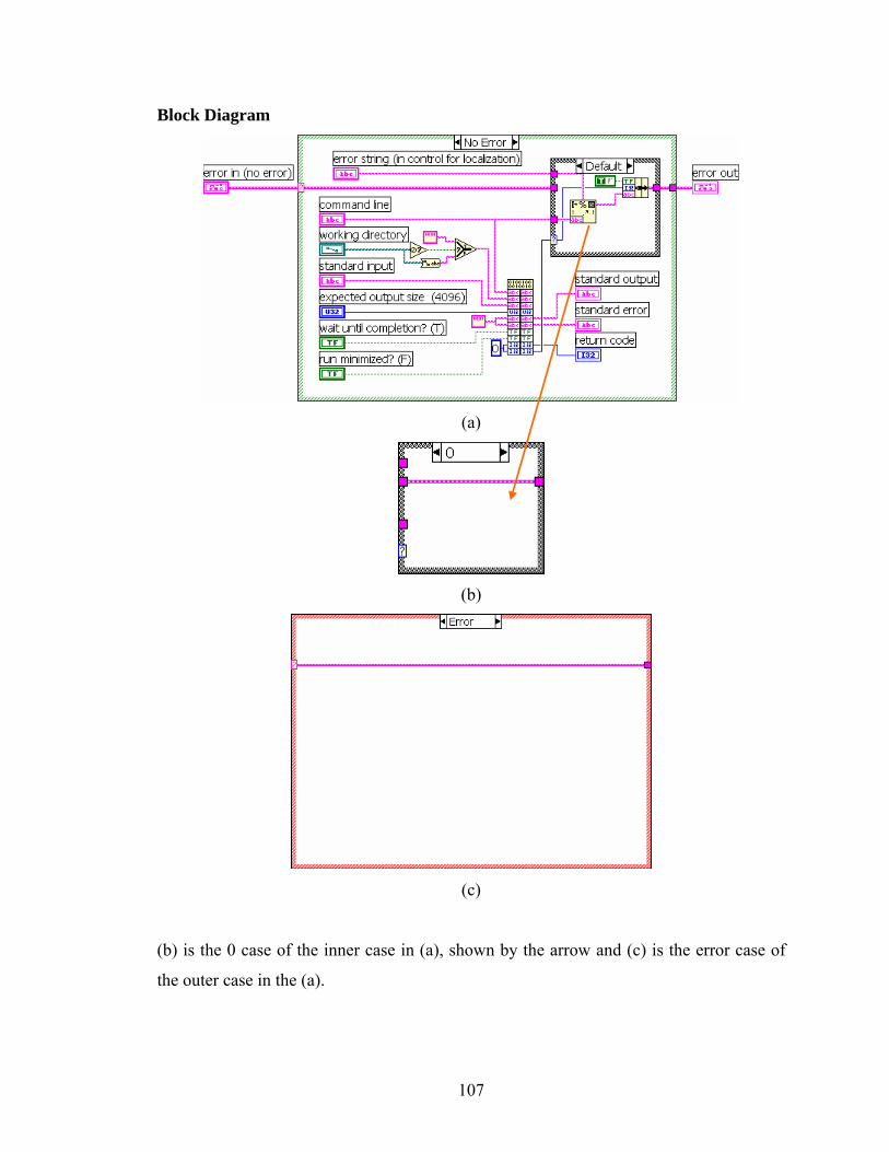
107
Block Diagram
(a)
(b)
(c)
(b) is the 0 case of the inner case in (a), shown by the arrow and (c) is the error case of
the outer case in the (a).

108
C.6 Write Characters To File.vi
Writes a character string to a new byte stream file or appends the string to an
existing file. The VI opens or creates the file before writing to it and closes it afterwards.
Please see LabView 6i help manual for more details.
Connector Panel
Front Panel
Block Diagram
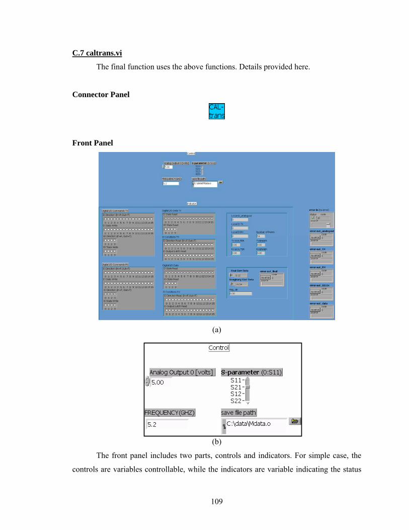
109
C.7 caltrans.vi
The final function uses the above functions. Details provided here.
Connector Panel
Front Panel
(a)
(b)
The front panel includes two parts, controls and indicators. For simple case, the
controls are variables controllable, while the indicators are variable indicating the status

110
of data flow, to give us an idea of how the flow is going on now. In part b, the controls
are 4 of them, Analog output 0 S parameter, Frequency in GHz, and save file path. The
default value is shown above too.
Block Diagram
(a)
(b)

111
TX16OUTER
TX8INNER
16
RX8INNER
65535
15
IO State WriteIO Direction (In=F, Out=T)
D State WriteD Direction (In=F,Out=T)
Digital I/O Commands RX
0000
error out_RX
D Conditions RX
Digital I/O Data RX
set D(i) high RX
1Local ID RX
IO State ReadD State Read
D Output Latch ReadD Direction Read (In=F,Out=T)
0 [0..3]
RX16OUTER
1
8
65535
Local ID TX0
set D(i) high TX
Digital I/O Commands TX
15
65535
Digital I/O Data TX
D Conditions TX
error out_TX
0000
IO State WriteIO Direction (In=F, Out=T)
D State WriteD Direction (In=F,Out=T)
IO State ReadD State Read
D Output Latch ReadD Direction Read (In=F,Out=T)
8
1
65535
16
(c)
RX8INNER
65535
15
IO State WriteIO Direction (In=F, Out=T)
D State WriteD Direction (In=F,Out=T)
Digital I/O Commands RX
0000
error out_RX
D Conditions RX
Digital I/O Data RX
set D(i) high RX
1Local ID RX
IO State ReadD State Read
D Output Latch ReadD Direction Read (In=F,Out=T)
0 [0..3]
RX16OUTER
1
8
65535
16
(d)

112
(a) is the schematic of the block diagram (b), as we compare them, we notice that
the three parts are displayed as initialization, taking measurement and running the image
algorithm. In (b) 3 blocks are illustrated, the block before the loops is the initialization,
the loops are taking measurement and the block after it is to run the image algorithm.
Now we see the close-ups of those blocks and we mark them with numbers so that the
flow can be illustrated. (c) is the overall measurement taking part, and (d) is the inner
loops of receiving antenna arrays. Inside(c), it contains (d) part and a block before (d)
part to set the transmitting antenna arrays. In (d), inside the two loops, there is a frame
structure, as what in (a), this frame has 2 functions, set the receiving antenna arrays and
take the s parameters. The frames are shown in the following steps.
C.8 Initialization
VISA session 2
error in (no error)dup VISA session 2
FREQUENCY(GHZ)
String 2
S-parameter (0:S11)
CENTGHZ; SPAN0HZ; SWEA; POIN3; LINFREQ; CHAN1;
Initilize network analyzer
0 [0..1]
(a) Step 1
10
wait 10ms
1 [0..1]
1Analog Output 0 [volts] Local ID_analogouterror out_analogout
set the analog output
error in_analogout
(b) Step 2
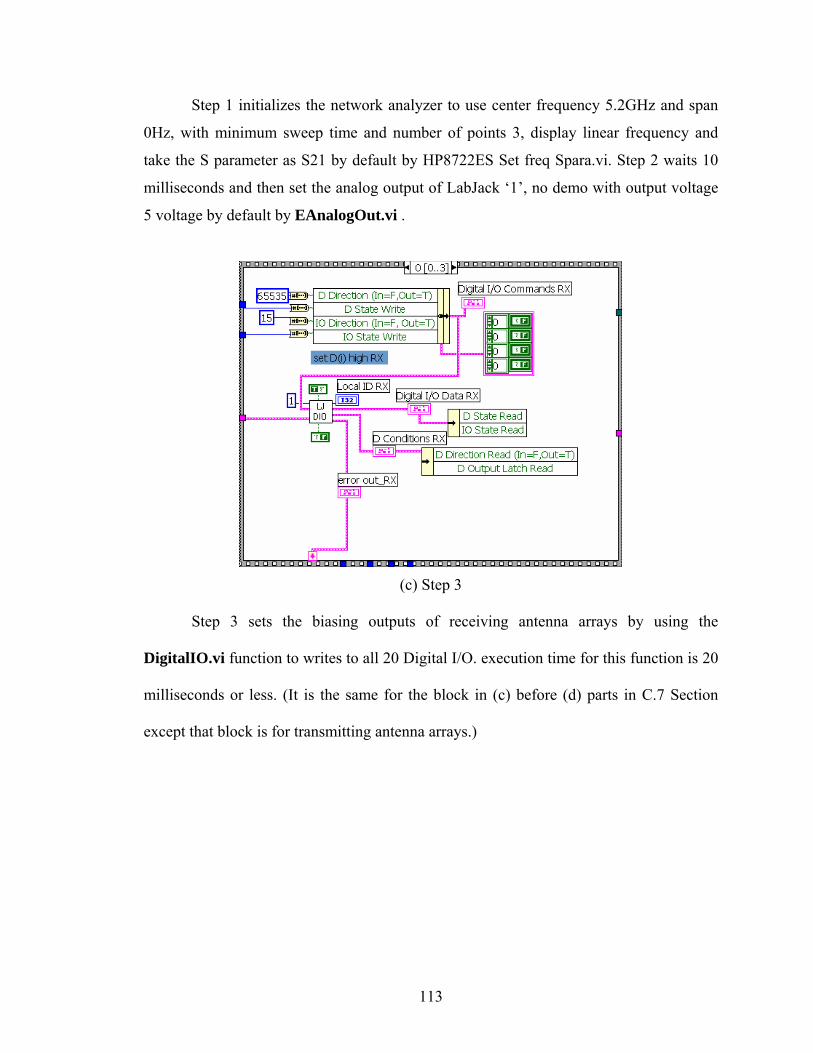
113
Step 1 initializes the network analyzer to use center frequency 5.2GHz and span
0Hz, with minimum sweep time and number of points 3, display linear frequency and
take the S parameter as S21 by default by HP8722ES Set freq Spara.vi. Step 2 waits 10
milliseconds and then set the analog output of LabJack ‘1’, no demo with output voltage
5 voltage by default by EAnalogOut.vi .
(c) Step 3
Step 3 sets the biasing outputs of receiving antenna arrays by using the
DigitalIO.vi function to writes to all 20 Digital I/O. execution time for this function is 20
milliseconds or less. (It is the same for the block in (c) before (d) parts in C.7 Section
except that block is for transmitting antenna arrays.)
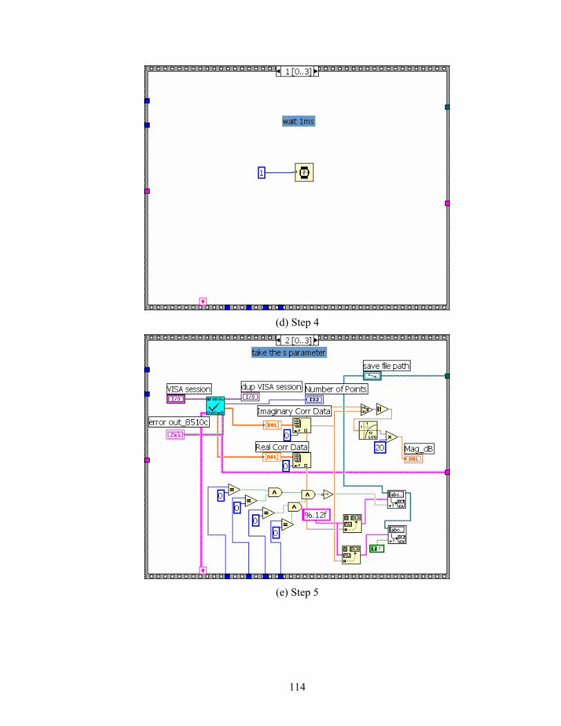
114
(d) Step 4
(e) Step 5

115
(f) Step 6
Step 4 waits 1 ms and step 5 takes the measurement data by using HP8510C
Output Corrected Data.vi. This function output real/imaginary pairs from selected
channel corrected data memory. Then data will be saved by Write Characters To File.vi.
Step 6 waits 1 ms.
run image algorithm
error out_finala=0
c:\data\nde3d.exe
error out_data
(g) Step 7
The 4-6 steps will be run for ‘128 times 128’ sequences, then the image algorithm
will be run by System Exec.vi at step 7 by. An image of the concrete will be generated
after that.


![0272 &/8% &$67(//$==2 %250,'$ VHOHWWLYD &DPSLRQDWR 1D ... Castellazzo... · 0272 &/8% &$67(//$==2 %250,'$ VHOHWWLYD &DPSLRQDWR 1D]LRQDOH 0RWRUDLG 02725$,' 6725,&2 *58332 5,(92&$=,21(](https://img.pdfslide.net/doc/110x75/5fc2af7b71528f695d5e46ec/0272-8-672-250-vhohwwlyd-dpslrqdwr-1d-castellazzo.jpg)