Embed Size (px)
Citation preview

�������� ����� ��
State-space independent component analysis for nonlinear dynamic processmonitoring
P.P. Odiowei, Y. Cao
PII: S0169-7439(10)00090-0DOI: doi: 10.1016/j.chemolab.2010.05.014Reference: CHEMOM 2233
To appear in: Chemometrics and Intelligent Laboratory Systems
Received date: 25 December 2009Revised date: 20 May 2010Accepted date: 21 May 2010
Please cite this article as: P.P. Odiowei, Y. Cao, State-space independent componentanalysis for nonlinear dynamic process monitoring, Chemometrics and Intelligent Labora-tory Systems (2010), doi: 10.1016/j.chemolab.2010.05.014
This is a PDF file of an unedited manuscript that has been accepted for publication.As a service to our customers we are providing this early version of the manuscript.The manuscript will undergo copyediting, typesetting, and review of the resulting proofbefore it is published in its final form. Please note that during the production processerrors may be discovered which could affect the content, and all legal disclaimers thatapply to the journal pertain.

ACC
EPTE
D M
ANU
SCR
IPT
ACCEPTED MANUSCRIPT
State-Space Independent Component Analysis for
Nonlinear Dynamic Process Monitoring
P.P. Odiowei and Y. Cao∗
School of Engineering, Cranfield University, Bedford, MK43 0AL, UK
This version: May 20, 2010
Abstract
The cost effective benefits of process monitoring will never be over emphasised.
Amongst monitoring techniques, the Independent Component Analysis (ICA) is an
efficient tool to reveal hidden factors from process measurements, which follow non-
Gaussian distributions. Conventionally, most ICA algorithms adopt the Principal
Component Analysis (PCA) as a pre-processing tool for dimension reduction and
de-correlation before extracting the independent components (ICs). However, due
to the static nature of the PCA, such algorithms are not suitable for dynamic pro-
cess monitoring. The dynamic extension of the ICA (DICA), similar to the dynamic
PCA, is able to deal with dynamic processes, however unsatisfactorily. On the other
hand, the Canonical Variate Analysis (CVA) is an ideal tool for dynamic process
monitoring, however is not sufficient for nonlinear systems where most measurements
follow non-Gaussian distributions. To improve the performance of nonlinear dynamic
process monitoring, a state space based ICA (SSICA) approach is proposed in this
work. Unlike the conventional ICA, the proposed algorithm employs the CVA as a
dimension reduction tool to construct a state space, from where statistically inde-
∗To whom all correspondence should be addressed, E-Mail: [email protected]
1

ACC
EPTE
D M
ANU
SCR
IPT
ACCEPTED MANUSCRIPT
pendent components are extracted for process monitoring. The proposed SSICA is
applied to the Tennessee Eastman Process Plant as a case study. It shows that the
new SSICA provides better monitoring performance and detect some faults earlier
than other approaches, such as the DICA and the CVA.
Keywords: Dynamic system, Nonlinearity, Principal component analysis, Canoni-
cal variate analysis, Independent component analysis, Probability density function,
Kernel density estimation, Process monitoring.
1 Introduction
Process monitoring techniques are employed to detect abnormal deviations of process
operation conditions and diagnose the causes for these deviations to maintain high
quality products and process safety. The Principal Component Analysis (PCA) is a
dimension reduction technique that summarises the variation in a set of correlated
variables to a set of de-correlated principal components (PCs), each of which is a linear
combination of the original variables. The PCA exploits the correlation amongst a
large number of measured variables and is popular for its simplicity. The PCA by
reducing the dimension of the process variables is able to eliminate noise and retain
only important process information. MacGregor and Kourti [1] established a PCA
model from the training data and judged the behaviour of online processes against the
PCA model to detect deviations from the normal operating process. Wang et al. [2]
also presented a PCA approach based on visualization using parallel co-ordinates
with the Manresa Waste Water Treatment Plant as a case study.
The widely applied PCA is a static approach that assumes that the observations are
in a steady-state, which is time independent. Furthermore, the PCA is normally
associated with the Hotelling’s T 2 statistic, which, in order to determine the upper
control limit, assumes that the principal components derived by the PCA follow a
Gaussian distribution. However, the assumption of time-independence may not be
valid for processes subject to dynamic disturbances. The assumption of normality
may also be invalid for most chemical processes where strong nonlinearity makes
2

ACC
EPTE
D M
ANU
SCR
IPT
ACCEPTED MANUSCRIPT
variables driven by noise and disturbances non-Gaussian. In these situations, the
PCA is not an appropriate tool for process monitoring.
A solution to address the limitation of Gaussian assumption associated with the PCA
is the Independent Component Analysis (ICA) [3–5]. The ICA technique recovers a
few statistically independent source signals from collected process measurements by
assuming that these independent signals are non-Gaussian. A set of variables are
said to be statistically independent from each other when the value of one vari-
able cannot be predicted by giving the value of another variable. Unfortunately in
process systems, such independent sources are in general not directly measurable,
but mixing each other in measurement variations. To identify the unmeasured ICs
from measurements, the ICA algorithm involves a pre-processing stage known as the
whitening stage to eliminate the cross correlation between the process variables before
extracting the independent components [3–10]. Although the ICA is sometimes con-
sidered as an extension of the PCA [3], the objectives of the ICA are clearly different
from those of the PCA. The ICA decomposes process measurements into statisti-
cally (high-order statistics) ICs of a lower dimension whereas the PCA decomposes
the process measurements into a set of de-correlated (second order statistics) PCs
of a lower dimension. Therefore, the ICA is able to extract more useful information
than the PCA [4, 5] and as a result performs better than the PCA based monitoring
techniques.
Process monitoring based on the ICA approach aims to extract the essential ICs, that
drive a process, for detecting underlying faults. Lee et al. [4] in their ICA approach
employed the Euclidean norm to determine the number of ICs to retain in the ICA
model. The ICs in the model space were described as the dominant ICs while the
ignored ICs were described as the excluded ICs. Three monitoring metrics; the I2d for
the dominant ICs, the I2e for the excluded ICs and the Q-metric for the residual space
were determined and then kernel density estimations (KDE) employed to derive the
control limit for all three statistics.
Albazzaz and Wang [8] in another way, employed all the extracted ICs for process
monitoring because it was argued that no single IC was more important than another.
In addition, a box-cox transformation was applied to change the non-Gaussian coor-
3

ACC
EPTE
D M
ANU
SCR
IPT
ACCEPTED MANUSCRIPT
dinates of the ICs to a Gaussian distribution in order to justify the use of the control
limits estimated based on the Gaussian assumption. Their technique was applied to
the Manresa Waste Water treatment plant in Spain to demonstrate its efficiency.
Conventionally, most published ICA studies have utilised the PCA for whitening and
dimension reduction in the pre-processing stage, allowing the ICs to be interpreted by
the simple geometry of the PCA [7]. However, the connection of the ICA with PCA
makes such ICA approaches not appropriate for dynamic process monitoring due to
the static nature of the PCA. For most industrial processes, variables driven by noise
and disturbances are strongly auto-correlated and time-varying making the PCA and
the ICA inappropriate for monitoring of such dynamic processes. This means that a
dynamic process would require a monitoring technique that will take the serial corre-
lations of the process data into account in order to achieve efficient dynamic process
monitoring. For this reason, Lee et al. [6] extended the ICA methods and proposed
the dynamic ICA (DICA) approach to improve the monitoring performance. In the
so called DICA approach, a dynamic extension of the PCA (DPCA) is applied to
an augmented data set in the pre-processing stage, where each observation vector is
augmented with the previous observations and stacked together to account for the
auto-correlations, then the ICs are extracted from the decomposed principal compo-
nents (PCs). However, the DICA, like the DPCA, is not the best approach to capture
the dynamic behaviour from process measurements [11]. As a result, the statistical
advantage of the ICA is not fully exploited by the DICA and the performance of the
DICA in dynamic process monitoring is still not satisfactory.
Nevertheless, the state-space models like the Canonical Variate Analysis (CVA) on
the other hand are reported to be efficient tools for dynamic process monitoring [11–
17]. The CVA is a dimension reduction technique that is based on state variables
and is well suited for auto-correlated and cross-correlated process measurements. This
makes the CVA based approaches a better choice than the PCA based approaches
for dynamic process monitoring. However, on the other hand, the states obtained
from the standard CVA, like the PCs are only de-correlated, but not statistically
independent, hence are not efficient enough for nonlinear process monitoring.
To derive an efficient tool for nonlinear dynamic process monitoring, in this paper,
4

ACC
EPTE
D M
ANU
SCR
IPT
ACCEPTED MANUSCRIPT
the CVA, rather than the PCA, is proposed as the pre-processing tool to associate
with the ICA resulting in a novel State Space ICA (SSICA) approach. In the ap-
proach, the CVA is adopted as a dimension reduction tool to construct a state space
and perform the dynamic whitening in the pre-processing stage. Then, the ICA is
applied to the constructed state space in order to identify the statistically indepen-
dent components. The SSICA approach is developed for nonlinear dynamic process
monitoring and applied to the Tennessee Eastman Process Plant as a case study.
It demonstrates that generally, the proposed SSICA is able to improve the process
monitoring performance over the existing DICA technique, which is reported to be an
improvement of the traditional ICA [6]. Also, the overall performance of the SSICA
is better than the CVA, which was reported to be an efficient dynamic monitoring
tool [11–17]. The performance improvements of the SSICA over the DICA and the
CVA include increases in detection reliability and decreases in both detection delay
and false alarms.
This paper is organised as follows: Section 2 describes the SSICA technique in details,
which include the CVA, SSICA and KDE algorithms. The SSICA is then applied to
the Tennessee Eastman Process Plant in section 3. Finally, this work is concluded in
section 4.
2 State Space Independent Component Analysis
The development of process monitoring techniques is geared towards applying these
techniques to industrial processes in order to improve process performance monitor-
ing. It is well known that most real time processes to which the monitoring techniques
are applied are dynamic and nonlinear. The SSICA approach is developed to deal
with such processes. Firstly, from a general nonlinear dynamic system, a linearized
state space model can be constructed from normal operation data through the CVA.
The non-Gaussian collective modelling errors are then extracted as statistically in-
dependent components through the SSICA. The obtained state space independent
components together with the residuals are used for process monitoring by compar-
ing the upper control limits estimated through the KDE approach. These algorithms
5

ACC
EPTE
D M
ANU
SCR
IPT
ACCEPTED MANUSCRIPT
are described in details as follows.
2.1 Canonical Variate Analysis
Consider a nonlinear dynamic plant represented as:
xk+1 = f(xk) + wk
yk = g(xk) + vk (1)
where xk ∈ Rn and yk ∈ Rm are state and measurement vectors respectively, f(·)
and g(·) are unknown nonlinear functions, whereas wk and vk are plant disturbances
and measurement noise vectors respectively. Clearly, it is difficult to monitor such
unknown nonlinear dynamic systems directly. Fortunately, under normal operation
conditions, the plant in Equation (1) can be approximated by a linear stochastic state
space model as:
xk+1 = Axk + εk
yk = Cxk + ηk (2)
where A and C are unknown state and output matrices respectively, whereas εk and
ηk are collective modelling errors partially due to the underlying nonlinearity of the
plant, which has not been included in the linear model, and partially associated with
process disturbance and measurement noise, wk and vk respectively. Note, as a result
of the nonlinearity of the physical plant represented in Equation (1), the collective
modelling errors, εk and ηk in Equation (2) generally will be non-Gaussian although
wk and vk might be normally distributed.
To monitor the linear dynamic process represented in (2) without knowing matrices
A and C, the CVA is employed to extract the state variables xk from process mea-
surements, yk. The CVA is based on the so called subspace identification, where the
process measurements are stacked to form the past and future spaces through the
past, yp,k and future, yf,k observations defined as follows.
6

ACC
EPTE
D M
ANU
SCR
IPT
ACCEPTED MANUSCRIPT
yp,k =
yk−1
yk−2
...
yk−q
∈ Rmq, yp,k = yp,k − yp,k (3)
yf,k =
yk
yk+1
...
yk+q−1
∈ Rmq, yf,k = yf,k − yf,k (4)
where the first subscripts of yp,k and yf,k indicate the past (p) and the future (f) ob-
servations respectively, whilst the second subscripts stand for the reference sampling
point, where the past and future observations are defined. The sample means of the
past and future observations are represented as yp,k and yf,k respectively, whilst yp,k
and yf,k are the pre-processed past and future observations with zero means.
The past and future truncated Hankel matrices Yp and Yf are then defined in Equa-
tion (5) and Equation (6) respectively.
Yp =[yp,(q+1) yp,(q+2) · · · yp,(q+M)
]∈ Rmq×M (5)
Yf =[yf,(q+1) yf,(q+2) · · · yf,(q+M)
]∈ Rmq×M (6)
From the Hankel matrices defined above, the covariance of the past, future and cross-
covariance matrices are estimated as follows:
Σpp = E(ypkyTpk) = YpY
Tp (M − 1)−1 (7)
Σff = E(yfkyTfk) = YfY
Tf (M − 1)−1 (8)
Σfp = E(yfkyTpk) = YfY
Tp (M − 1)−1 (9)
The goal of the CVA is to find the best linear combinations, aT yfk and bT ypk of the
future and past observations so that the correlation between these combinations is
maximised. The correlation can be represented as:
ρfp(a,b) =aTΣfpb
(aTΣffa)1/2(bTΣppb)1/2(10)
7
ACC
EPTE
D M
ANU
SCR
IPT
ACCEPTED MANUSCRIPT
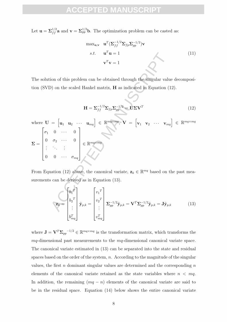
Let u = Σ1/2ff a and v = Σ
1/2pp b. The optimization problem can be casted as:
maxu,v uT (Σ−1/2ff ΣfpΣ
−1/2pp )v
s.t. uTu = 1 (11)
vTv = 1
The solution of this problem can be obtained through the singular value decomposi-
tion (SVD) on the scaled Hankel matrix, H as indicated in Equation (12).
H = Σ−1/2ff ΣfpΣ
−1/2pp = UΣVT (12)
where U =[u1 u2 · · · umq
]∈ Rmq×mq, V =
[v1 v2 · · · vmq
]∈ Rmq×mq
Σ =
σ1 0 · · · 0
0 σ2 · · · 0...
. . ....
0 0 · · · σmq
∈ Rmq×mq
From Equation (12) above, the canonical variate, zk ∈ Rmq based on the past mea-
surements can be derived as in Equation (13).
zk =
b1T
b2T
...
bTmq
yp,k =
v1T
v2T
...
vTmq
Σ−1/2pp yp,k = VTΣ−1/2
pp yp,k = Jyp,k (13)
where J = VTΣpp−1/2 ∈ Rmq×mq is the transformation matrix, which transforms the
mq-dimensional past measurements to the mq-dimensional canonical variate space.
The canonical variate estimated in (13) can be separated into the state and residual
spaces based on the order of the system, n. According to the magnitude of the singular
values, the first n dominant singular values are determined and the corresponding n
elements of the canonical variate retained as the state variables where n < mq.
In addition, the remaining (mq − n) elements of the canonical variate are said to
be in the residual space. Equation (14) below shows the entire canonical variate
8

ACC
EPTE
D M
ANU
SCR
IPT
ACCEPTED MANUSCRIPT
space (zk ∈ Rmq) is spanned by the state variables (xk ∈ Rn) and the residuals
(dk ∈ Rmq−n), both of which are subsets of the canonical variate, zk.
zk =[xk
T dkT]T
(14)
The previous work [17] showed that the state variables, xk obtained through CVA
provides a tool better than directly using the past or future observations to monitor
the dynamic systems in (1). However, as shown in (2), the states are combinations
of statistically independent non-Gaussian sources. To make process monitoring more
efficient, identifying these sources from the states is desired. The corresponding
algorithm is to be developed in the next section.
2.2 State Space Independent Component Analysis
According to (2), xk can be expressed as a linear combination of the initial state, x0
and the collective modelling errors, εj, for j = 0, 1, . . . , k − 1.
xk = Akx0 +k−1∑j=0
Ajεk−1−j (15)
Equation (15) indicates that if x0 and εj, j = 0, . . . , k − 1 are mixtures of m(≤ n)
unknown independent components, sj ∈ Rm, for j = 0, · · · , k − 1, then the states,
xk, for k = 1, . . .M are also linear combinations of these unknown independent
components. More specifically, the relationship can be expressed as follows.
X = BxSx (16)
where X =[x1 · · · xM
]∈ Rn×M is the state matrix, Bx =
[b1 · · · bm
]∈ Rn×m
is an unknown mixing matrix, and Sx =[sx,0 . . . sx,M−1
]∈ Rm×M is unknown
independent component matrix. The SSICA aims to estimate both mixing matrix, Bx
and independent component matrix, Sx, from the state matrix, X obtained through
the CVA as described above.
The problem can be solved through an existing ICA algorithm, such as the Fas-
tICA [18] to find a de-mixing matrix, W such that the rows of the estimated inde-
pendent component matrix,
Sx = WxX (17)
9

ACC
EPTE
D M
ANU
SCR
IPT
ACCEPTED MANUSCRIPT
are as independent of each other as possible. Based on the “non-Gaussian repre-
sents independence” principle [18], the de-mixing matrix as well as the independent
component matrix are obtained through iterative optimizations to maximize certain
non-Gaussian criteria.
The ICA can be applied to the residual space spanned by dk. The independent
component matrix in the residual space is obtained by applying the ICA algorithm
to the residual matrix, D as follows.
Sd = WdD (18)
where D =[d1 · · · dM
]∈ R(mq−n)×M .
The ICA based process monitoring is frequently associated with the Mahalanobis
distance I2, also known as the D-statistic [4, 6, 10]. The I2 metric is the sum of the
squared independent components extracted from the ICA algorithm.
I2x,k = sTx,ksx,k (19)
I2d,k = sTd,ksd,k (20)
where sx,k and sd,k are the k-th columns of S and Sd, respectively. The M I2x,k and I2
d,k
values for k = 1, . . . ,M are then used to derived the upper control limits, I2x,UCL(α)
and I2d,UCL(α) using the KDE algorithm described in the next section.
For online monitoring, the ICs of the state and residual spaces is calculated from the
new measurements, ynewp,k using the transformation matrix, J =
[JTx JTd
]Tand the
de-mixing matrices, Wx and Wd respectively.
snewx,k = WxJxy
newp,k (21)
snewd,k = WdJdy
newp,k (22)
The corresponding I2 metrics for the new measurements are then obtained as follows.
I2,newx,k = (snew
x,k )T snewx,k (23)
I2,newd,k = (snew
d,k )T snewd,k (24)
A fault condition is then detected if either I2 metric is larger than the corresponding
UCL.
10

ACC
EPTE
D M
ANU
SCR
IPT
ACCEPTED MANUSCRIPT
2.3 Control Limit Through Kernel Density Estimations
The ICs are not Gaussian. Therefore, the UCL for the I2 metric cannot be derived
analytically. The kernel density estimation (KDE) is a well established approach to
estimate the PDF of random processes [19–21]. Hence, it is a natural selection using
the KDE to determine the UCL [17]. Considering both I2 metrics are positive, a
KDE algorithm with lower bound support is adopted in this work to estimate the
UCL.
Let y > 0 be the random variable under consideration. Firstly, the bounded y is
converted into unbounded x by defining x = ln(y). Then, the density function p(x)
can be estimated by the normal KDE algorithm. Finally, the density function of y is
p(ln(y))/y as derived in (25).
P (y < b) = P (x < ln(b)) =
∫ ln(b)
−∞p(x)dx =
∫ b
0
p(ln(y))1
ydy (25)
Therefore, by knowing p(x), an appropriate control limit can be determined for a
specific confidence bound, α using Equation (25). The estimation of the probability
density function p(x) at point x through the kernel function, K(·) is defined as follows
p(x) =1
Mh
M∑k=1
K
(x− xkh
). (26)
where xk, k = 1, 2, · · · ,M are samples of x and h is the bandwidth. The bandwidth
selection in KDE is an important issue because selecting a bandwidth too small will
result in the density estimator being too rough, a phenomenon known as under-
smoothed while selecting a bandwidth too big will result in the density estimator
being too flat. There is no single perfect way to determine the bandwidth. However,
a rough estimation of the optimal bandwidth hopt subject to minimising the approx-
imation of the mean integrated square error can be derived in Equation (27), where
σ is the standard deviation [22].
hopt = 1.06σN−1/5 (27)
To use both I2x and I2
d metrics together, the joint distribution of these two metrics
11

ACC
EPTE
D M
ANU
SCR
IPT
ACCEPTED MANUSCRIPT
has to be considered. In general, the joint probability of two random variables, x and
y is defined as follows.
P (x < a, y < b) =
∫ a
−∞
∫ b
−∞p(x, y)dxdy (28)
However, for the SSICA and the DICA, I2x and I2
y are independent. Hence,
P (x < a, y < b) = P (x < a)P (y < b) (29)
Equation (29) can also be approximately applied to T 2 and Q metrics for the CVA
because x and d in (14) are uncorrelated [23]. This means the joint PDF estimation
can be simplified by two univariate PDF estimations.
By replacing xk in Equation (26) with I2x,k and I2
d,k obtained in (19) and (20) respec-
tively, the above KDE approach is able to estimate the underlying PDFs of the I2x
and I2d metrics. The corresponding control limits, I2
x,UCL(α) and I2d,UCL(α) can then
be obtained from the PDFs of the I2x and I2
d metrics for a given confidence level, α
by solving the following equations respectively.
∫ I2x,UCL(α)
0
p(ln(I2x))
I2x
dI2x
∫ I2d,UCL(α)
0
p(ln(I2d))
I2d
dI2d = α (30)∫ I2x,UCL(α)
0
p(ln(I2x))
I2x
dI2x =
√α (31)∫ I2d,UCL(α)
0
p(ln(I2d))
I2d
dI2d =
√α (32)
In this work, a fault is then identified (Fk = 1) if either I2,newx,k > I2
xUCL(α) or I2,newx,d >
I2dUCL(α) conditions are satisfied, i.e.
Fk = (I2,newx,k > I2
x,UCL(α))⊕ (I2,newd,k > I2
d,UCL(α)) (33)
where ⊕ represents a logical “OR” operation.
12

ACC
EPTE
D M
ANU
SCR
IPT
ACCEPTED MANUSCRIPT
3 APPLICATION - Tennessee Eastman Process
Plant
The Tennessee Eastman Process (TEP) plant has 5 main units which are the reactor,
condenser, separator, stripper and compressor [13, 24, 25]. A graphical description
of the TEP plant is presented in Figure 1.
XC
XF
XE
XF
XH
XE
XD
XG
11C4
5
6
8
9
12
Condenser
FI
TI
PI
LI
JI
TI
FI
A
N
A
L
Y
Z
E
R
XA
XB
XC
XD
XE
XF
Compressor
Stripper
Vap/Liq
separator
7
A
PCFI
1
CWS
13CWR
CWS
PI
TI
FI
SC
TI
CWR
Cond
FI
Stm
TI
10
FI
LI
Purge
A
N
A
L
Y
Z
E
R
LI
Reactor
PI
FI
FI
Product
XBA
N
A
L
Y
Z
E
R
XA
XD
XH
XG
PCFI
2D
3E
PCFI
Figure 1 Graphical Description of the TEP Plant
The TEP process is a large dimensional, nonlinear process with unknown mathemat-
ical representation as the simulation is intentionally distributed as an undocumented
FORTRAN program [24, 25]. The TEP data consists of two blocks; the training and
test data sets each of which has 22 continuous process measurements, 12 manipulated
variables and 19 composition measurements sampled with time delays. There are also
21 scenarios corresponding to Faults 0 − 20, with Fault 0 being the data simulated
at normal operating condition (no fault) and Faults 1 - 20 corresponding to data sets
13

ACC
EPTE
D M
ANU
SCR
IPT
ACCEPTED MANUSCRIPT
from the simulated fault processes, each with a specified fault as listed in Table 1.
Table 1 Brief Description of TEP Plant Faults
Fault Description Type
1 A/C Feed Ratio, B Composition Constant (Stream 4) Step
2 An increase in B while A/C Feed ratio is constant (stream 4) Step
3 D Feed Temperature (Stream 2) Step
4 Reactor Cooling Water Inlet Temperature Step
5 Condenser Cooling Water Inlet Temperature Step
6 A loss in Feed A (stream 1) Step
7 C Header Pressure Loss - Reader Availability (Stream 4) Step
8 A,B,C Feed Composition (Stream 4) Random variation
9 D Feed Temperature (Stream 2) Random variation
10 C Feed Temperature (Stream 4) Random variation
11 Reactor Cooling Water Inlet Temperature Random variation
12 Condenser Cooling Water Inlet Temperature Random variation
13 Reaction Kinetics Slow drift
14 Reaction Cooling Water Valve Sticking
15 Condenser Cooling Water Valve Sticking
16 Unknown Unknown
17 Unknown Unknown
18 Unknown Unknown
19 Unknown Unknown
20 Unknown Unknown
A total of 52 measurements are collected for each data set of length, N = 960
representing 48-hour operation with a sampling rate of 3 minutes. Among these mea-
surements, 19 analyzer measurements, 14 of which are sampled at 6 minute interval
whilst other 5 are sampled in every 15 minutes, have not been included in this study
due to the measurement time delay, while 11 manipulated variables are treated the
same as other measured variables because under feedback control, these variables are
not independent any more. The simulation time of each operation run in the test
data block is 48 hours and the various faults are introduced only after 8 hours. This
means that for each of the faults, the process is in normal operation condition for the
14

ACC
EPTE
D M
ANU
SCR
IPT
ACCEPTED MANUSCRIPT
first 8 simulation hours before the process becomes abnormal after the introduction
of the fault. Furthermore, all twenty TEP faults have also been studied to investi-
gate the effectiveness of the proposed SSICA technique. The results are based on a
α = 99% confidence level (√α = 0.995 for individual metrics).
The TEP plant is under closed-loop control, which by its nature, tries to overcome
the abnormal deviations that occur as a result of the introduction of the various faults
to the simulated TEP process. Due to the closed loop nature of the plant, deviations
caused by some faults are relatively small such that these faults are difficult to be
detected by most monitoring approaches, such as principal component analysis and
partial least squares [17]. Different from these conventional methods, the SSICA
proposed in this work aims to address both dynamic and nonlinear issues effectively.
The monitoring performance in this study is assessed by the percentage reliability,
which is defined as the percentage of the samples outside the control limits [26].
Hence, a monitoring technique is said to have a better performance over another if
the percentage reliability of this technique is numerically higher than the percentage
reliability of another technique. Another criterion employed in this study to judge
the performance of the monitoring techniques is the detection delay, which is how
long it takes for a technique to identify a fault after the introduction of the fault.
A monitoring technique is said to be better than another if it is able to detect a
fault earlier than another technique. The false alarm rate, which is the percentage of
samplings classified as abnormal during the 8 hour normal operation period before
introducing a fault, is also considered for performance comparison.
To demonstrate the efficiency of the proposed SSICA, the monitoring performance
of the proposed SSICA is compared with the monitoring performance of the DICA
technique, an existing dynamic extension of the ICA. The SSICA is also compared
with the CVA to demonstrate the improvement by performing ICA on the state space
obtained by the CVA. For the pre-processing CVA described above, the number of
state variables to retain in the dominant space is normally determined by the dom-
inant singular values from the scaled Hankel matrix H in Equation (32). However,
applying the CVA to the TEP case study showed that using the dominant singular
values left an unrealistically large number of state variables in the dominant space.
15
ACC
EPTE
D M
ANU
SCR
IPT
ACCEPTED MANUSCRIPT
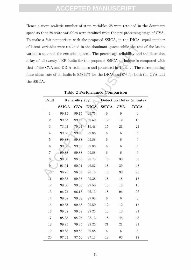
Hence a more realistic number of state variables 28 were retained in the dominant
space so that 28 state variables were retained from the pre-processing stage of CVA.
To make a fair comparison with the proposed SSICA, in the DICA, equal number
of latent variables were retained in the dominant spaces while the rest of the latent
variables spanned the excluded spaces. The percentage reliability and the detection
delay of all twenty TEP faults for the proposed SSICA technique is compared with
that of the CVA and DICA techniques and presented in Table 2. The corresponding
false alarm rate of all faults is 0.6849% for the DICA and 0% for both the CVA and
the SSICA.
Table 2 Performance Comparison
Fault Reliability (%) Detection Delay (minute)
SSICA CVA DICA SSICA CVA DICA
1 99.75 99.75 99.75 9 9 9
2 99.63 99.63 99.50 12 12 15
3 73.03 70.04 19.48 15 21 21
4 99.88 99.88 99.88 6 6 6
5 99.88 99.88 99.88 6 6 6
6 99.88 99.88 99.88 6 6 6
7 99.88 99.88 99.88 6 6 6
8 99.00 98.88 98.75 18 30 33
9 91.64 90.01 46.82 18 39 48
10 96.75 96.38 96.13 18 90 96
11 99.38 99.38 99.38 18 18 18
12 99.50 99.50 99.50 15 15 15
13 96.25 96.13 96.13 18 96 96
14 99.88 99.88 99.88 6 6 6
15 99.63 99.63 99.50 12 12 15
16 99.38 99.38 99.25 18 18 21
17 98.38 98.25 98.13 18 45 48
18 99.25 99.25 99.25 21 21 21
19 99.88 99.88 99.88 6 6 6
20 97.63 97.50 97.13 18 63 72
16

ACC
EPTE
D M
ANU
SCR
IPT
ACCEPTED MANUSCRIPT
The superiority of the SSICA over the CVA and DICA techniques is demonstrated
in Table 2. For 10 of the 20 faults (2,3,8,9,10,13,15,16,17 and 20), the SSICA is able
to improve the monitoring performance over the existing DICA technique in both
reliability and detection delay, while for the rest 10 faults, the SSICA maintains the
same performance as the DICA does. This is achieved by the SSICA with a reduced
false alarm rate for all faults. In the reliability, the improvement of the SSICA over
the DICA is significant (> 0.5%) for 4 of the faults (3,9,10 and 20). Particularly,
for faults 3 and 9, the improvement is extremely significant, over 40%. Meanwhile,
the SSICA is able to reduce the detection delay significantly (> 10 minutes) for 6
faults (8, 9, 10, 13, 17 and 20). The over one hour reduction in detection delay
is achieved by using the SSICA on faults 10 and 13. In comparison between the
SSICA and CVA, the performance of the SSICA is better than that of the CVA for
7 faults (3, 8, 9 10, 13, 17 and 20) in both the reliability and the detection delay,
whilst these performance criteria of the remaining 13 faults are the same for both
methods. In the reliability, the improvement on 2 faults (3 and 9) are significant (over
1%). Meanwhile, significant improvements in the detection delay (> 10 minutes) are
observed for 6 faults (8, 9, 10, 13, 17 and 20), for two of which (10 and 13), the
improvements are over one hour.
To appreciate the capability of the SSICA, fault detection by these three methods
along with fault propagation is further analysed for Faults 3 and 9. As shown in
Table 1, both Faults 3 and 9 relate to the temperature of D feed (stream 2), one
for step change (Fault 3) and another for random variations (Fault 9). These faults
directly result in small deviations in the reactor cooling water outlet temperature,
which can be easily corrected by the closed-loop control system by manipulating the
cooling water flow. Therefore, both faults are generally difficult to be detected by
most monitoring approaches.
Figure 2 shows a comparison of the fault detection along with the propagation of
Fault 3 for the SSICA (a), CVA (b) and DICA (c) techniques, using Fk derived from
Equation (33), whilst Figure 3 shows the fault detection along with the propagated
Fault 9 process for these three techniques.
17

ACC
EPTE
D M
ANU
SCR
IPT
ACCEPTED MANUSCRIPT
8 16 24 32 40 480
0.5
1
(a) SSICA 73.0337 % Relability, 15 minute detection delayF
k
8 16 24 32 40 480
0.5
1
(b) CVA 70.0375 % Relability, 21 minute detection delay
Fk
8 16 24 32 40 480
0.5
1
(c) DICA 19.4757 % Relability, 21 minute detection delay
Fk
time, hour
Figure 2 Comparison of fault detection along with the propagation of Fault
3
18

ACC
EPTE
D M
ANU
SCR
IPT
ACCEPTED MANUSCRIPT
8 16 24 32 40 480
0.5
1
(a) SSICA 91.6355 % Relability, 18 minute detection delayF
k
8 16 24 32 40 480
0.5
1
(b) CVA 90.0125 % Relability, 39 minute detection delay
Fk
8 16 24 32 40 480
0.5
1
(c) DICA 46.8165 % Relability, 48 minute detection delay
Fk
time, hour
Figure 3 Comparison of fault detection along with the propagation of Fault
9
It is for such faults as Faults 3 and 9 that the superiority of the proposed SSICA
technique over the CVA and particularly the DICA techniques is most outstanding
as illustrated in Figure 2 and Figure 3. The performance of the SSICA is better
than that of the CVA and DICA techniques for both Faults 3 and 9. Particularly,
it is clear that for both faults the SSICA is able to show a significant improvement
of fault detection over the DICA technique within a few hours of the early stage of
fault propagation. The improvement in the early fault propagation stage is important
since it will give more time for operators to deal with the detected fault.
Although the DICA, also referred to as the ICA with delays is reported to be a more
efficient dynamic monitoring tool than the traditional ICA [6], the proposed SSICA
technique is able to significantly improve the monitoring performance over the DICA
technique for most of the faults considered in this work. This is because the pre-
processing stage of the SSICA is based on the CVA, which is a more appropriate
19

ACC
EPTE
D M
ANU
SCR
IPT
ACCEPTED MANUSCRIPT
dynamic monitoring tool than the DPCA on which the DICA technique is firstly based
on. Furthermore, the efficiency of the SSICA over the CVA is owed to the fact that the
SSICA is more suited than the CVA to deal with non-Gaussian process measurement,
separating the original sources to a greater degree than the CVA technique. The
results illustrated above demonstrate that there were no faults for which either the
CVA or DICA techniques outperformed the proposed SSICA technique.
It is worth to note that the CVA approach adopted in this work is able to cope with
certain level of nonlinearities due to the use of the KDE to determine the UCL [17].
Moreover, the superiority of the CVA over the DICA indicates that the dynamic issue
has more impact on the fault detection performance than the nonlinearity for the TE
process. This might be due to the feedback control, which widely propagates the
transient response caused by a fault, as well as restricts the variations caused by a
fault to relatively small level. This restriction on variation causes some faults to be
difficult to detect without taking into account the correlations in time. Meanwhile,
the effect of nonlinearity on fault responses is also restricted so that the CVA with
KDE approach is able to detect most faults adequately. This may also be the reason
for most faults the performance of the SSICA and the CVA is very close.
4 Conclusion
In this study, an ICA model was developed based first on CVA in the pre-processing
stage before applying the ICA algorithm and then control limits derived based on
kernel density estimations with 99% joint confidence intervals. The proposed ap-
proach is applied to the Tennessee Eastman Process. The monitoring performance
of the proposed SSICA is assessed and compared with those of the CVA and DICA
techniques also considered in this study. The percentage reliability, detection delays
as well as the false alarm rates were adopted to assess and compare the monitoring
performance of the proposed approach with those of the CVA and DICA techniques.
The percentage reliability of the SSICA was significantly higher than both of the
DICA and the CVA for some of the faults although the significance of improvement
over the CVA was not as high as that over the DICA. Moreover, the SSICA is also
20

ACC
EPTE
D M
ANU
SCR
IPT
ACCEPTED MANUSCRIPT
able to dramatically reduce the detection delay over both the CVA and the DICA
for certain faults. In particular, the remarkable superiority of the SSICA is demon-
strated in the faults that are more difficult to detect, emphasizing the efficiency of
the proposed SSICA over the existing CVA and DICA techniques.
References
[1] MacGregor, J. F., and Kourti, T., 1995. “Statistical process control of multi-
variate processes”. Control Engineering Practice, 3(3), pp. 403–414.
[2] Wang, X. Z., Medasani, S., Marhoon, F., and Albazzaz, H., 2004. “Multidi-
mensional visualization of principal component scores for process historical data
analysis”. Industrial Engineering Chemical Research, 43, pp. 7036–7048.
[3] Abazzaz, H., and Wang, X. Z., 2004. “Statistical process control charts for batch
operations based on independent component analysis”. Industrial & Engineering
Chemistry Research, 43(21), pp. 6731–6741.
[4] Lee, J., Yoo, C., and Lee, I., 2004. “Statistical process monitoring with inde-
pendent component analysis”. Journal of Process Control, 14, pp. 467–485.
[5] Chen, G., Liang, J., and Qian, J., 2004. “Chemical process monitoring and fault
diagnosis based on independent component analysis”. In 5th World Congress on
Intelligent Control and Automation, p. 1646.
[6] Lee, J., Yoo, C., and Lee, I., 2004. “Statistical monitoring of dynamic indepen-
dent component analysis”. Chemical Engineering Sciences, 59, pp. 2995–3006.
[7] Lee, J., Qin, S. J., and Lee, I., 2006. “Fault detection and diagnosis based on
modified independent component analysis.”. AIChE Journal, 52(10), pp. 3501–
3514.
[8] Albazzaz, H., and Wang, X. Z., 2006. “Historical data analysis based on plots
of independent and parallel coordinates and statistical control limits.”. Journal
of Process Control, 16, pp. 103–114.
21

ACC
EPTE
D M
ANU
SCR
IPT
ACCEPTED MANUSCRIPT
[9] Liu, X., Xie, L., Kruger, U., Littler, T., and Wang, S., 2008. “Statistical-based
monitoring of multivariate non-gaussian systems analysis.”. AIChE Journal,
54(9), pp. 2379–2391.
[10] Hongguang, L., and Hui, G., 2006. “The application of independent component
analysis in process monitoring.”. In Proceedings of the 1st International Con-
ference on Innovative Computing, Information and Control (ICICIC06), p. 97.
[11] Negiz, A., and Cinar, A., 1998. “Monitoring of multivariable dynamic processes
and sensor auditing”. Journal of Process Control, 8(56), pp. 357–380.
[12] Juan, L., and Fei, L., 2006. “Statistical modelling of dynamic multivariate
process using canonical variate analysis”. In Proceedings IEEE International
on Information and Automation, 2006. ICIA 2006, p. 218.
[13] Chiang, L. H., Russell, E. L., and Braatz, R. D., 2001. Fault Detection and
Diagnosis in Industrial Systems. Springer, London.
[14] Simouglou, A., Martin, E. B., and Morris, A. J., 2002. “Statistical performance
monitoring of dynamic multivariate processes using state space modelling”. Com-
puters and Chemical Engineering, 26, pp. 909–920.
[15] Larimore, W. E., 1983. “System identification reduced order filtering and mod-
elling via canonical correlation analysis”. In Proceedings of the American Control
Conference, p. 445.
[16] Negiz, A., and Cinar, A., 1997. “Pls, balanced and canonical variate realization
techniques for identifying varma models in state space”. Chemometrics and
Intelligent Laboratory Systems, 38, pp. 209–221.
[17] Odiowei, P., and Cao, Y., 2009. “Nonlinear dynamic process monitoring using
canonical variate analysis and kernel density estimations”. IEEE Transactions
on Industrial Informatics, 6(1), pp. 36–45.
[18] Hyvarinen, A., 1999. “Fast and robust fixed-point algorithms for independent
component analysis”. IEEE Transactions on Neural Networks, 3, pp. 626–634.
22

ACC
EPTE
D M
ANU
SCR
IPT
ACCEPTED MANUSCRIPT
[19] Chen, Q., Kruger, U., Meronk, M., and Leung, A. Y. T., 2004. “Synthesis of
t2 and q statistics for process monitoring”. Control Engineering Practice, 12,
pp. 745–755.
[20] Bowman, A. W., and Azzalini, A., 1997. Applied Smoothing Techniques for
Data Analysis, The Kernel Approach with S-Plu Illustrations. Clarendon Press,
Oxford.
[21] Martin, E. B., and Morris, A. J., 1996. “Non-parametric confidence bounds
for process performance monitoring charts”. Journal of Process Control, 6(6),
pp. 349–358.
[22] Xiaoping, S., and Sonali, A., 2006. “Kernel density estimation for an anomaly
based intrusion detection system”. In Proceedings of the 2006 World Congress
in Computer Science, Computer Engineering and Applied Computing, p. 161.
[23] Chen, Q., Krunger, U., Meronk, M., and Leung, A., 2004. “Synthesis of t2
and q statistics for process monitoring”. Control Engineering Practice, 12,
pp. 745–755.
[24] Ricker, N. L., 2001. Tennessee eastman challenge archive.
[25] Downs, J. J., and Vogel, E., 1993. “A plant-wide industrial process control
problem”. Computers and Chemical Engineering, 17, pp. 245–255.
[26] Kano, M., Koji, N., Shinji, H., Ioro, H., Hiromo, O., Ramon, S., and Bhavik,
R. B., 2002. “Comparison of multivariate statistical process monitoring methods
with applications to the eastman challenge problem”. Computers and Chemical
Engineering, 26, pp. 161–174.
23