Embed Size (px)
Citation preview

S1. Embodied energy in the Anglo-Danish Trade 1870-1913: methods, sources
and data
Sofia Henriques and Paul Warde
1. General discussion of methods and sources
This Supplementary Information explains how we have reconstructed embodied energy in the Anglo-
Danish trade over the period 1870-1913. We can divide traded goods into two types: energy (i.e food
and fuels) and non-energy (i.e. paper, iron). In our work, the term embodied energy in a traded good
refers to the energy content of the traded good plus the ’hidden’ energy requirements to extract and
produce the traded good and its inputs. We measure energy in terms of Gigajoules per metric tonne
(GJ/t)
There are two components in the energy embodied in trade: Energy and Hidden Energy. Energy
goods have energy content, which is measured in net calorific values in the case of fuels (oil
products, coal, coke, firewood, charcoal) and in metabolizable values in case of food. Both energy
and non-energy goods have Hidden Energy. Hidden energy refers to the quantities of energy which
are needed to produce the traded product. It is a net product, so in the case of Energy goods it
includes only the transformation losses that occur in the process of the conversion from the primary
energy of coal into coke or electricity, or of feed into livestock products such as eggs, bacon and
butter. The term hidden energy requirement is thus slightly different from the term total energy
requirements, since the term total energy requirements does include all coal used in the production
of electricity (both the energy to be found transformed into the electricity, and that which is lost in
generating it).
Energy goods can consist of primary energy carriers or secondary energy carriers. Primary energy
carriers are fuels such as coal, crude oil and biomass (firewood, feed and crops). 1 See below for a
further discussion of our definitions. Secondary energy carriers are livestock products and other
processed foods, coke, electricity and oil products.
1.1 The basic method of calculating hidden energy in goods
We have used a version of ‘Process analysis’ (Bullard et al. 1978) that relates all of the material inputs
to a final product, including those that are consumed in the manufacture and are not physically
present in the final product itself (whether combusted or discarded as residual waste). It is important
1
1

to be clear about the various steps in the production process as obviously errors could skew the
results.
We have traced the input-output relationships in physical terms, and calculated embodied energy
inputs per metric tonne of good (GJ/t). Nevertheless, a degree of aggregation is inevitable given the
quality of the data. Generally we have attempted to get as close to the disaggregated production of
goods as is possible.
The first step in this kind of process analysis is to determine the inputs required to produce a traded
good. Typically these inputs will include direct energy requirements, such as coal in smelting metal,
and goods and raw materials from other industries. The energy input into the final stage of
production represents the direct energy requirement. Each non-energy input is then further
examined to identify energy and non-energy inputs required for its production. This process
continues to the point where the inputs are believed to add a negligible amount to the total energy
use. To take a very simple example, to calculate the hidden energy in one tonne of cotton yarn we
must calculate the energy inputs into producing raw cotton as a first step, and then the energy inputs
into spinning as a second (the full details of how this is done are provided below). However, for each
tonne of cotton yarn produced, there is some wastage, so more than one tonne of raw cotton was
required to produce each tonne of cotton yarn. Hence the energy inputs into a tonne raw cotton
must be multiplied by 1.08 (reflecting losses of around 6-8%) to get the hidden energy requirements
from raw cotton that went into a ton of cotton yarn. Of course, most products have more than one
input. The sum of energy inputs to all the stages of extraction, processing and production prior to the
final stage of production the final good are known as the indirect hidden energy requirements. Adding
the direct and indirect energy requirements yields the total hidden energy requirements for the
production of one unit (a metric tonne) of a target product. In the case of energy goods like food and
fuel, the embodied energy also includes their own energy content, which is not hidden.
It is also very important to note again that at each step in any production process we must also
remember to include the indirect hidden energy that went into producing the energy supply. For
example, each 100 hundred tons of coal required around 6 tons of coal to be burned at mines for its
extraction. This means that every ton of coal introduced at any point in the production process must
be multiplied by 1.06 to provide the full tonnage actually required to produce a good. Energy also has
‘hidden energy’, just as any raw material or intermediary input.
The list below only includes those sectors or categories of product that have been calculated because
of their significance in embodied energy flows in trade between Britain and Denmark. Thus the data
coverage is uneven between benchmark years, partly for reasons of the structure of inputs (whether
2

they were sourced from home or abroad), partly for reasons of relevance to the issued of energy
embodied in trade, and partly because of data availability.
2. The Energy System
There is a very large literature on the definition of the energy system and different approaches to its
analysis. The total energy system of course relies on a constant flow of inputs from the sun and
ongoing transformations throughout the natural world. We take a more limited view typical in
economic analysis, in that we define our system boundaries according to energy inputs into
economic activity that have some kind of opportunity cost in terms of the allocation of labour
(human time), land (allocation of land use to productive activity) and capital (equipment required to
capture energy flows). Even with this definition boundary-setting is not a simple matter, as we
discuss below.
Sorman and Giampietro (2013) use a typical distinction between Primary Energy Sources and Energy
Carriers. Energy carriers are those energy inputs which enter into economic activity, while ‘Primary
Energy Sources are needed to generate the supply of Energy Carriers used’. In some cases these are
identical; coal and oil can be both an Energy Carrier and a Primary Energy Sources. Electricity is
however never a Primary Energy Source, but must be generated by transforming other forms of
energy: coal, oil, wind, water, etc. However, even these simple definitions contain, as Sorman and
Giampietro (2013) concede, a ‘chicken and egg’ problem. In practice, few energy analyses
incorporate solar radiation as the original Primary Energy Source; in practice they adopt a more
limited, economically-orientated definition as we have done. Equally, in most cases any Primary
Energy Source requires the earlier use of Energy Carriers for its exploitation. Capturing wind using a
windmill requires previous energy investments in the mill, possibly made decades before; using a
steam engine requires the manufacture of all of its parts at some earlier date. In practice it is
impossible to allocate all of these inputs from Energy Carriers over time to individual traded goods,
and even less possible to allocate such inputs to Primary Energy Sources, which represents an
endless, recursive series of inputs back in time.
We discuss the boundary setting we have adopted in the next two sections. Because of the different
challenges involved, we distinguish between the industrial and the agricultural systems.
2.1. Industrial system
The energy inputs into the industrial system we analyze include direct data on coal and coke
consumption and estimates of the use of oil, water power and indirect coal consumption from
purchased electricity derived from data on installed power equipment. In the British industrial
3

systems of the late 19th and early 20th century, coal was overwhelmingly dominant, representing 98-
99% of energy inputs for most products. Hence in 1870 we have not, in many cases, allocated energy
inputs from water power; they would make no difference to our results.
The list above refers to Energy Carriers. To convert these into Primary Energy inputs we include the
all the energy sued within the extractive sector and electricity generation to mine coal and produce
electrical power. The Primary Energy input into water power is the energy contained in water hitting
the wheel. The Primary Energy input into gas (in this period coal rather than natural gas) is the coal
used in its production; this is also calculated in the case of coke. Oil, being a very small part of the
energy system, has not been converted into Primary Energy (i.e. including energy used for
extraction).
We have not calculated the energy inputs required to produce capital goods that were then used in
production. In practice, this would be extremely difficult to allocate accurately. Equally, in examining
historical data, there would a danger in double-counting. If we included energy embodied in capital
goods in our calculations, the energy embodied in machinery being imported from Britain to
Denmark, for example should, from an extremely strict consumption-based accounting point of view,
be allocated as embodied energy to all of the future products of that machinery. Allocating
embodied energy would thus require knowledge of all future production to avoid double-counting.
Instead we use the normal procedures of economic accounting in treating each year as a single cycle
of production, tracing the consumption and flows of that one year, even though this clearly always
requires the setting of rather artificial boundaries.
2.2. The Agricultural System
We consider as energy inputs the primary energy sources which were required for the production of
a given good. The Primary Energy Sources considered as inputs are firewood, coal, oil, primary
electricity, direct water and wind and feed, both for draught animals, and as an input for the
production of livestock products. For this period and two countries, animal feed and coal are the
most important sources. As with the Industrial system, data refers to Energy Carriers, and must be
converted into Primary Energy Sources as appropriate.
Calculating energy flows in the agricultural system is, appropriately enough, particularly prone to the
chicken-and-egg problem. The production of feed for livestock usually requires, besides solar
radiation, inputs of machinery, tools, fertilizer, further feed for livestock that work to produce more
feed, and so on. Generally speaking these inputs were produced in an earlier cycle of production that
allowed the feed to be produced as an input into the current cycle (although clearly this division of
4

the economy into neat, discrete cycles of production is artificial). Such chicken-and-egg problems
have the potential to pull us endlessly back in time. To avoid this problem we treat feed for draught
animals as a Primary Energy Source, and we do not additionally allocate energy inputs required to
produce feed to the goods that the use of that feed allowed to be produced. This is possible due to
the conceptual separation of agriculture output into crops (requiring insolation, fertilizers and animal
labour) and pastures2 (requiring only insolation), see Figure 1. We make the simplifying assumption
to attribute to draught animals feed from pastures so to avoid endlessly recurrent addition of hidden
energy in the feed per working animals.
Figure 1. System boundaries in accounting for embodied energy in Danish agriculture products
2.3 Outside the boundaries
As in any study of embodied energy, some methodological decisions had to be made in order to
simplify the analysis. Here, we discuss the possible impact of changing the boundaries to our model.
2 Pastures include hay and grass in crop rotation.
5

2.3.1. Human labour as an energy input
In this work trade we do not measure labour as an energy input to the production of a product, i.e.,
as part of hidden energy. We limit ourselves to calculating the energy content of the traded food and
the hidden inputs for its production, i.e. feed and fuels. One reason is simplicity, given that it would
add further data demands to our model. The second reason for avoiding calculating food for humans
as an input is the accuracy of allocation and our understanding of the production function. Unlike
animals, the sole purpose of human existence is not working, so there is controversy on which
measure of energy to use as representative of their work (Fluck 1992). For some, energy inputs
related to human work should only include the increase in food intake that occurs due to working
activity (although this would require some rather rough estimation). This would exclude the energy
requirements for body survival and leisure activities, for instance. If we took this approach the
amount of energy embodied in human labour compared with other inputs would be insignificant.
Others would suggest including the energy consumed by people during working hours (Stanhill
1980), and others would suggest to take into account all energy expenditure during the day. But
would this still matter for our results? In 1913, when Danish exports were booming, the food
consumed by the whole agricultural working population was approximately 2.5 PJ 3. No more than
half this value should be involved in the trade with the UK 4. This is only a small proportion of the food
consumption in Denmark in that year (14.3 PJ) and a very small proportion of the energy hidden in
exports in that year (54PJ). More inclusive measures, will also include as an indicator of human
labour the food necessary to sustain families across the life-cycle (Pimentel and Pimentel 2008) with
even higher values if the embodied energy in food would also be taken into account, but this type of
approach suffers from problems of circularity. In addition, if this data were utilized in conventional
economic analysis, where the question of substitution between different factors of production arises,
including both embodied energy in human labour, and labour as a factor of production, introduces
double-counting. It is, of course, perfectly legitimate to take any of these measures as part of an
analysis but we have not done so here and it would not affect our results.
2.3.2. Transport energy
Obviously, traded goods must be transported, and transport has an energy cost. There can be little
doubt that the rapid growth in trade between 1870 and 1913 was facilitated by increased use of
3 Considering that the per capita food consumption of Denmark was 4.6 GJ/year (Henriques and Sharp 2016) and that the amount of workers employed in the agriculture was 531 thousand ( Hansen 1984).4 In a previous version of this work we have performed a simple calculation that allocates food for workers accordingly to the amounts’ of feed given to the animals and the value obtained was around 1.2 PJ.
6

steam ships and railways. We do not explicitly measure the impact of transport of goods between
Denmark and the UK, although in principle, we already account for the balance of energy used for
this purpose. If ships (of any nationality) which transported British coal and industrial products
bunkered in the UK, the coal necessary for the transport of products to Denmark would not be
registered as an export to Denmark (as it would probably be registered as supply for bunkers
involved in foreign trade, according to the practice of British statistics). However, the coal necessary
for the transport of Danish products to the UK would most likely be a part of Britain’s coal exports to
Denmark, if we assume that ships which exported Danish products to the United Kingdom bunkered
in Denmark. Assuming that the coal necessary to transport Danish exports would be roughly the
same as that to transport Danish imports, our work would already account for this balance as a
component of energy imports to Denmark. These transport costs would not, of course, be attributed
to particular goods. How important would be the total embodied energy in maritme transport? We
do not have enough information to know this exactly. The quantity of coal recorded as going into
Danish bunkers in 1913 is 110 000 t (SD 1960). Knowing that two thirds of the exports in value were
going to the UK, and if we assumed that around the same proportion of coal was going to boats with
Britain as a final destination, and with the assumption that the quantity necessary for exports is
roughly the same as for imports5 then we obtain a total value of 140 0000 t for transportation
requirements between the countries, roughly 4 PJ. This is very small in comparison to the total
energy embodied in the trade between the two countries. Of course the different characteristics of
the cargoes and the role of Denmark as an importer-exporter of grain from other parts of the world
could change the amount of energy used in this trade, but determining a more precise value would
require a whole new study.
2.3.3 Feed for non-working animals
We have only measured the feed for working animals and feed for non-working animals that was
embodied in food products. This was because these were the flows with an impact in the Anglo-
Danish trade. In theory, our model could be enlarged to extend the analysis of feed to products such
as wool, although this would create the problem of separating by-products such as meat from wool
in allocating energy.6 In practice this would not have a significant impact in our results as the net
balance of the wool trade between the two countries was a mere hundred tonnes.
5 This assumption is not implausible, even taken into consideration that Danish exports weighted much less than British imports- the same amount of ships was travelling between the two countries. There is an ideal cargo weight that would balance the ship- lighter ships would normally have to be filled with water in the deck, so that the ship would not sink. 6 Jensen (1937) discusses that wool was a byproduct of meat in Denmark, since the receipts where much larger for meat than for woolen products.
7

3. Embodied energy intensities: Denmark and the UK 1870-1913
Because of the different sources employed, and at times different methodological challenges, we
have divided our discussion of methods to calculate energy requirements into a section on Denmark
and a section on Britain. In practice, of course, both countries had inputs from abroad, as will be
discussed below. Most importantly, coal was an essential energy input into Denmark and
considerable amounts were imported from Britain.
3.1 Calculating embodied energy intensities for Danish export products
This sections aims at give a more comprehensive account of the steps needed to arrive at the
estimations of embodied energy intensities of butter, bacon and eggs. To do that we had to follow
three steps, as can be seen in Figure 2:
Step 1. Quantifying energy inputs for crop outputs,
Step 2. Calculating the different hidden energy intensities of the various types of crop output and
imported feed (maize, oil cakes) which were consumed by cattle, poultry and pigs.
Step 3. Calculating embodied energy intensities of livestock products by a) quantifying the amounts
and composition of feed per type of animal b) allocating the total amount of embodied energy in
animal nutrition to the different livestock products c) accounting for energy embodied in the
industrial processes.
Figure 2. Accounting for embodied energy in Danish livestock products
8

Step 1. Quantifying energy inputs for crop-outputs
Fuels, electricity use and feed for draught animals
Our point of departure for the historical estimation of fuel and electricity use in agriculture is data for
1936 from Schroll (1984), translated to 1913 using a simple estimation. For instance, we have
estimated the consumption of electricity assuming that the share of agriculture in total electricity use
was the same in 1913 as in 1936 (37%). Electricity was converted into primary coal equivalents using
the ratio of 76 GJ/MWh, taking into account the energy use in the power stations and coal mining
(Statens Kulforholdene 1921; SD 1916a). Fuel use between 1913 and 1936 is assumed to vary at the
same rate as fertilizer use. For the year 1870 there were very few steam engines in agriculture and
for this reason energy from fuels was not estimated. Finally, we use Henriques and Sharp’s (2016)
estimation of feed for draught animals as a measure of work from animals in Danish agriculture.
Energy for Fertilizers
In 1870, Danish agriculture employed negligible amounts of synthetic fertilizers. In 1913, there were
four main groups of fertilizers used in Danish lands: Chilean nitrates, calcium nitrate,
superphosphates and potassium fertilizers. Energy requirements for Chilean nitrate extraction are
registered in the Statistical Yearbook of Chile (OCE 1914) and include the use of coal, oil and animal
energy.7 Calcium nitrate fertilizers, with a 15.5% N concentration, were imported from Norway.
Norway produced nitrates by using the Birkeland-Eyde process, an antecessor of the Haber-Bosh
7 We thank Kristin Ranestad for providing us access to this data.
9

process which was highly energy-intensive, requiring large amounts of cheap hydro-power. The
energy requirements of the process are quantified in Warming (1923). Superphosphates are
obtained from treating rock phosphate with sulfuric acid, phosphoric acid or a mixture of the two.
Danish superphosphates had 18% concentration. Although Denmark produced superphosphates, we
were unable to gather information on its production. We have taken the embodied energy intensities
in generic fertilizers from the US (US, 1917) – mostly superphosphates – as representative values 8.
Finally, we use the energy requirements to produce 1 t of stone-salt from the UK, as a good indicator
of energy embodied in potassium fertilizers. The average embodied energy in Danish fertilizers in
1913 was 7.7 GJ/t.
Step 2. Calculating the hidden energy intensities of different crops and oil cakes
Domestic crops
Having obtained the total quantities of animal labour, fertilizers and fuels embodied in the Danish
agriculture we can start to allocate them to the various crop-outputs. The first step to do this is to
define which crops receive the inputs of draught animals, fuels and fertilizers. Our cropland area
includes the area used to grow wheat, rye, oats, barley, mixed grains, pulse, beet sugar and root
crops (potato, turnips, carrots, among others). It excludes forests, pastures and the area for growing
hay and grass, even if part of a crop rotation. This is based on the idea that one does not need much
animal labour, fuels and fertilization to grow grass and hay. Having defined the cropland area, it is
assumed that working animals, fuels and fertilizers, are equally distributed across cropland. Of
course, this is a simplification made necessary due to the lack of more detailed data - as some crops
used more animal energy than others, or more fertilizers, or were more mechanized. For a country
like Denmark, with most of the crop devoted to animal feed, it seems a reasonable assumption.
Having obtained a hidden energy intensity per hectare (GJ/ha), and knowing the physical
productivities of the different crops (in t/ha), it is possible to express the hidden energy intensities in
GJ per t of each individual crop. Finally, the energy content, i.e. metabolizable energy of the crop in
GJ/t, is added to the crop hidden energy intensities to obtain the embodied energy intensities of crop
products.
8 Besides energy inputs in order to calculate the embodied energy for fertilizers we needed to calculate the energy embodied in a variety of raw materials: salts, pyrite, sulphuric acid, phosphate rock, etc.
10

Foreign crops
For simplicity, we have assumed that foreign grain had the same embodied energy intensities as
domestic grain. The only exception to this rule is maize, which was not produced domestically. The
maize coefficient is calculated from data from the United States ( Carter et al. 2006), following the
same procedure as for Danish crops to obtain the quantity of animal power embodied in 1 t of maize.
For 1913, these figures were adjusted to account for mechanization and use of fertilizers. These were
based on Danish figures: for example, in Denmark in 1913 energy and fertilizers will increase the
hidden energy/tonne ratio figures by 18% in comparison with accounting only for animal power.
Oil cakes
Oil cakes are important feed concentrates, the solid component of which results from the pressing of
any type of oil seeds. They were mostly fed to the cows. There were three main types of oil cakes
imported by Denmark in the period: cotton-seed cakes (United States), sun-flower cakes (Russia) and
flax-seed cakes (Russia and Germany). We were able to collect information on the GJ/t of oil cakes
from the USA for 1909 and 1914, which we use as representative of conditions in 1876 and 1913 (US,
1917), respectively. A majority of the US exports of oil cakes went to Denmark, with US oil cakes
taking up 42% of all cake imports in 1900. Most of the raw materials of oil cake production are
residuals from agriculture (i.e cotton seed) or byproducts of other industries. For these reasons, we
treat as important only the energy used directly in the production process.
Step 3. Calculating the embodied energy intensities of livestock products
The last, and more complex step is to calculate the embodied energy intensities of livestock
products. The livestock products (butter, meat, eggs and bacon) are complex products because the
energy embodied in them depends not only on feed requirements per t of product, but also on the
feed composition. Animal nutrition can be derived from pastures, different types of grains and root
crops, and by-products such as skimmed milk or oil cakes. As all these products have different
embodied energy intensities, it is necessary to know both the quantities of feed required for each
type of animal (cow, hen and pork) and the type of nutrition.
Allocation of nutrition per class of animal9
To determine the amounts of nutrition per class of livestock, our point of departure is
contemporaneous estimations of the amount of and type of crops, measured in metabolizable
energy, which were going to feed animals for both 1876 (Lindhard 1926) and 1913 (SD 1968, 1969).
9 We thank Paul Sharp for providing us literature and suggestions on this section.
11
The feed was then allocated per group of animals with basis in their standardized livestock units
(SLU). The SLU are based on the fodder consumption of animals of all types in relation to a milch cow.
This relation was estimated on the basis of a survey of feeding practices in Denmark in 1934-1936 (SD
1969). We assume that the relation was stable across years, see Figure 3. The feed requirements per
SLU have grown substantially from 20 GJ/SLU in 1876 to 28/SLU in 1913.
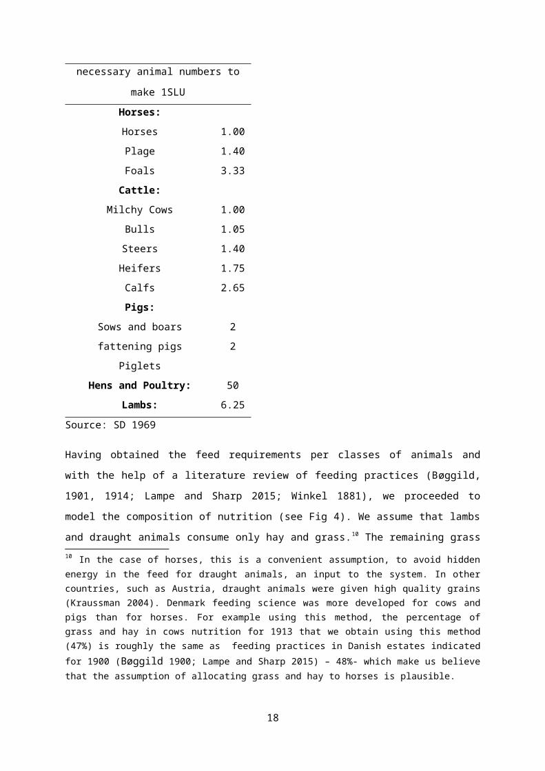
Fig 3. Standardized Livestock units conversion factors
necessary animal numbers to make 1SLU
Horses:
Horses 1.00
Plage 1.40
Foals 3.33
Cattle:
Milchy Cows 1.00
Bulls 1.05
Steers 1.40
Heifers 1.75
Calfs 2.65
Pigs:
Sows and boars 2
fattening pigs 2
Piglets
Hens and Poultry: 50
Lambs: 6.25
12

Source: SD 1969
Having obtained the feed requirements per classes of animals and with the help of a literature review
of feeding practices (Bøggild, 1901, 1914; Lampe and Sharp 2015; Winkel 1881), we proceeded to
model the composition of nutrition (see Fig 4). We assume that lambs and draught animals consume
only hay and grass.10 The remaining grass and hay output is allocated to the cows. Oil cakes are only
given to the cows. Skimmed milk is distributed to both cows and pigs according to the literature, i.e,
55% to pigs and 45% to cows in 1876 and 75% to pigs and 25% to cows in 1913. With the remaining
grain and root crops it was possible to make an approximation of the likely requirements for cows
and pigs.
Fig 4. Feed composition by class of animal 1876 and 1913
1876 1913 1876 1913 1876 1913 1876 1913Cattle Pigs Chicken Others
0.0
10.0
20.0
30.0
40.0
50.0
60.0
Skimmed milk Oil cakes Grass Root crops Grain
PJ
One final adjustment to the data in hand is needed, due to the fact that animals were fed skimmed
milk. Skimmed-milk is a by-product from the separation of cream from milk to make butter, that is, a
product of the nutrition of the cow. Skimmed milk was given to calfs and increasingly to pigs, so that
contemporaneous dairy accounts would describe pigs as products of cows. To avoid some inevitable
10 In the case of horses, this is a convenient assumption, to avoid hidden energy in the feed for draught animals, an input to the system. In other countries, such as Austria, draught animals were given high quality grains (Kraussman 2004). Denmark feeding science was more developed for cows and pigs than for horses. For example using this method, the percentage of grass and hay in cows nutrition for 1913 that we obtain using this method (47%) is roughly the same as feeding practices in Danish estates indicated for 1900 ( Bøggild 1900; Lampe and Sharp 2015) – 48%- which make us believe that the assumption of allocating grass and hay to horses is plausible.
13

double counting that would result from this, and relate the amounts of energy in feed with crops
outputs, we have performed the following adjustments to the data:
1) Skimmed milk is not counted as part of nutrition of the cows. When skimmed milk is given to
pigs we deduct this from the total feed from cows.
2) When skimmed milk is given to pigs, only the energy content of skimmed milk is accounted
for. The energy required to make skimmed milk is allocated to the cow, because the sole
reason why skimmed milk exists is butter production11. The transfer of skimmed milk from a
cow to pig can be seen as if the skimmed milk was measured in terms of grass, as pastures
and grass and hay crops have in our model a hidden energy intensity of zero.
Figure 5 shows the adjusted energy content of the nutrition considered, for cattle, pigs and chicken
and the associated hidden energy of this nutrition described in step 2.
Figure 5. Embodied energy in feed for Cattle, Pigs and Poultry
1876 1913 1876 1913 1876 1913Cattle Pigs Chicken
0.05.0
10.015.020.025.030.035.040.045.050.0
Hidden energy in feed Feed, adjusted*
PJ
Note: *These are final adjusted values. To allocate the feed of cows to butter and meat, we use first the total
quantities of grass, rootcrops, grain and oil cakes ingested. The skimmed milk transfer to pigs is only made after
the milk/meat allocation is done.
Having estimated the nutrition of the groups of livestock in which we are interested ( cattle, pigs and
chicken) and the energy embodied in their nutrition, it is now possible to begin the allocation of
these figures to the English Breakfast ( butter, eggs and bacon).
From Pigs to Pork and bacon
There is information on the joint production of pork and bacon for 1876 and 1913 (SD, 1969,
Lindhard, 1926), 44 000 and 231 000 t, respectively. For 1876 we have simply divided the energy
embodied in the nutrition for pigs by the tonnes of product to obtain the energy embodied in 1 t of 11 Skim-milk had a negligible economic value.
14

pork and bacon, 115 GJ/t. For 1913, we have added to the energy embodied in the nutrition, the coal
consumption in the slaughterhouses. This was estimated on the basis of the total horse power of
motors employed in the slaughterhouses, 5774 HP, assuming that the engines had an efficiency of 3%
(equal to the efficiency of industry generally). The energy embodied in 1 ton of pork and bacon
product in 115 GJ/t in 1876 and is equal to 142.4 GJ/t in 1913.
From Poultry to eggs
The products of this class of animals are meat and eggs. There is information in the production of
poultry meat and eggs for the period 1913 (SD, 1969) and a rough estimation for the period 1876
(Lindhard, 1926).12 In order to allocate the embodied energy in nutrition to the two products we
have converted the energy content of each product to GJs and then we assumed that the energy
embodied in the nutrition of poultry was distributed across the two type of products, according to
their share of GJ. In terms of GJ, the contribution of eggs is 74% in 1876 and 79% in 1913. The
embodied energy in eggs is 194 GJ/t in 1876 and 234 GJ/t in 1913.
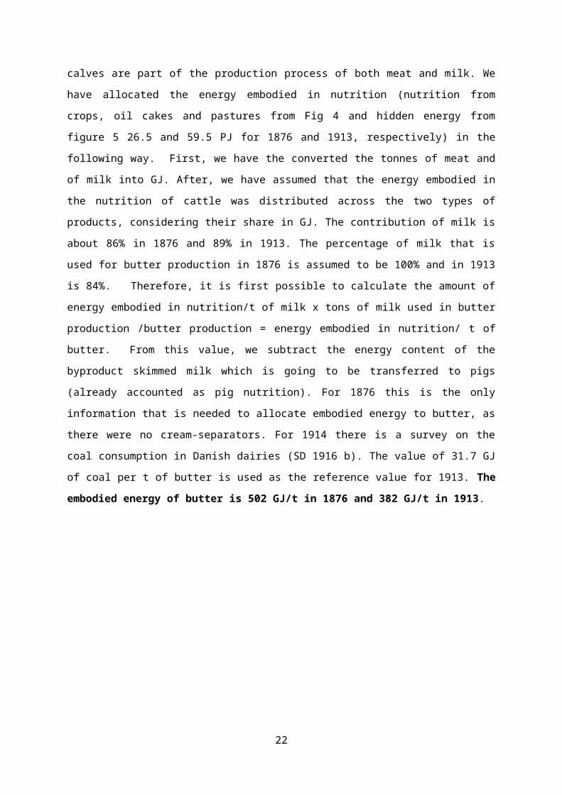
From Cattle to butter
There is information in the production of meat and milk and there is also information in the usage of
milk for butter production as opposed to the other uses (SD, 1969; Lindhard, 1926). Bulls and calves
are part of the production process of both meat and milk. We have allocated the energy embodied in
nutrition (nutrition from crops, oil cakes and pastures from Fig 4 and hidden energy from figure 5
26.5 and 59.5 PJ for 1876 and 1913, respectively) in the following way. First, we have the converted
the tonnes of meat and of milk into GJ. After, we have assumed that the energy embodied in the
nutrition of cattle was distributed across the two types of products, considering their share in GJ. The
contribution of milk is about 86% in 1876 and 89% in 1913. The percentage of milk that is used for
butter production in 1876 is assumed to be 100% and in 1913 is 84%. Therefore, it is first possible to
calculate the amount of energy embodied in nutrition/t of milk x tons of milk used in butter
production /butter production = energy embodied in nutrition/ t of butter. From this value, we
subtract the energy content of the byproduct skimmed milk which is going to be transferred to pigs
(already accounted as pig nutrition). For 1876 this is the only information that is needed to allocate
embodied energy to butter, as there were no cream-separators. For 1914 there is a survey on the
coal consumption in Danish dairies (SD 1916 b). The value of 31.7 GJ of coal per t of butter is used as
the reference value for 1913. The embodied energy of butter is 502 GJ/t in 1876 and 382 GJ/t in
1913.
12 There were only registers from poultry since 1898, in opposition with other animals.
15

3.2 Calculating embodied energy intensities for British exports
This section contains the detailed calculations for the main exports of the United Kingdom to
Denmark. In practice these goods were almost entirely produced within Britain and not Ireland, and
the data refers to Britain only. This material is excerpted from a larger work on estimates of energy
embodied in trade, here dealing with two benchmark points. The main sources are the Report of the
Royal Commission on Coal that was published in 1871 (HMSO, 1871), which included in its Appendix
E either estimates or collected data on the level of coal consumption in particular industries; and the
first Census of Production taken in 1907 (HMSO, 1913). Because British goods were in part
manufactured from raw materials and intermediary products from overseas, the Royal Commission
and Census of Production cannot be the only sources of data. Where necessary this is discussed in
the case of particular products.
Coal
All years: Coal consumed in mines can simply be related to total coal production to produce a hidden
energy intensity. The energy necessary to mine the coal is 1870: 1.91 GJ/t and 2 GJ/t for 1907. The
embodied energy of coal is 31 GJ/t.
Iron Ores
1870: Direct data on coal inputs into iron ore mining are not available. For later periods (see below)
the hidden energy requirements for iron ore mining have been calculated as being 0.2-0.6 GJ/ton in
16

Britain and 0.2 GJ/ton in Sweden. I have used the figure calculated for British ironstone mines in
1907, i.e. the top of this range.
1907: Within this sector some 6.802 million tons or iron ore and ironstone were raised (although a
larger amount of 8 million tons was also recorded under the coalmining sector, a very small share of
the total output of this sector). This used 137 580 tons of coal, producing a embodied energy
intensity of 0.609 GJ/ton.
Pig Iron and ferrous alloys
1870: Step 1: In principle the first step take the energy requirements for iron ore mining and
calculate the ratio of iron ore inputs in relation to final pig iron output. The energy requirements
estimated are reported above, and statistics collected by the British Iron and Steel Federation
indicate that the ratio of ore inputs to pig iron output in 1873 was 2.57 (British Iron & Steel
Federation 1949)13
Step 2: Fuel consumed by blast furnaces in the production of pig iron was estimated by the Royal
Commission on Coal (report published in 1871), and direct data was collected from 1873 and is
reported by the British Iron and Steel Federation. The working estimate of 1871 was 3 tons (imperial)
of coal consumed per ton of pig iron but the direct reports of 1873 give a rather lower figure of 2.56
tons. The latter, directly reported figure has been preferred (British Iron & Steel Federation 1949) .
The total energy requirement for pig iron is thus 80.9 GJ/t
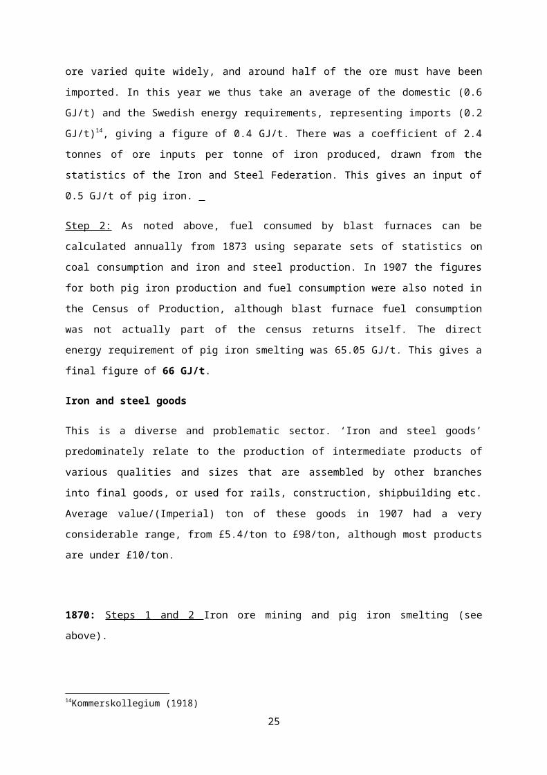
1907: Step 1: In principle the first step take the multiplier for iron ore mining and calculate the
coefficient of iron ore in relation to final pig iron output. However the quality and source of ore
varied quite widely, and around half of the ore must have been imported. In this year we thus take
an average of the domestic (0.6 GJ/t) and the Swedish energy requirements, representing imports
(0.2 GJ/t)14, giving a figure of 0.4 GJ/t. There was a coefficient of 2.4 tonnes of ore inputs per tonne of
iron produced, drawn from the statistics of the Iron and Steel Federation. This gives an input of 0.5
GJ/t of pig iron.
Step 2: As noted above, fuel consumed by blast furnaces can be calculated annually from 1873 using
separate sets of statistics on coal consumption and iron and steel production. In 1907 the figures for
both pig iron production and fuel consumption were also noted in the Census of Production,
13
14Kommerskollegium (1918)
17
although blast furnace fuel consumption was not actually part of the census returns itself. The direct
energy requirement of pig iron smelting was 65.05 GJ/t. This gives a final figure of 66 GJ/t.
Iron and steel goods
This is a diverse and problematic sector. ‘Iron and steel goods’ predominately relate to the
production of intermediate products of various qualities and sizes that are assembled by other
branches into final goods, or used for rails, construction, shipbuilding etc. Average value/(Imperial)
ton of these goods in 1907 had a very considerable range, from £5.4/ton to £98/ton, although most
products are under £10/ton.
1870: Steps 1 and 2 Iron ore mining and pig iron smelting (see above).
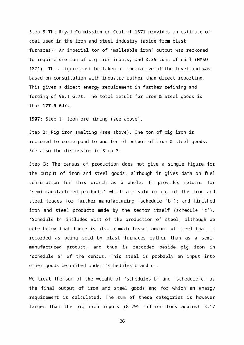
Step 3 The Royal Commission on Coal of 1871 provides an estimate of coal used in the iron and steel
industry (aside from blast furnaces). An imperial ton of ‘malleable iron’ output was reckoned to
require one ton of pig iron inputs, and 3.35 tons of coal (HMSO 1871). This figure must be taken as
indicative of the level and was based on consultation with industry rather than direct reporting. This
gives a direct energy requirement in further refining and forging of 98.1 GJ/t. The total result for Iron
& Steel goods is thus 177.5 GJ/t.
1907: Step 1: Iron ore mining (see above).
Step 2: Pig iron smelting (see above). One ton of pig iron is reckoned to correspond to one ton of
output of iron & steel goods. See also the discussion in Step 3.
Step 3: The census of production does not give a single figure for the output of iron and steel goods,
although it gives data on fuel consumption for this branch as a whole. It provides returns for ‘semi-
manufactured products’ which are sold on out of the iron and steel trades for further manufacturing
(schedule ‘b’); and finished iron and steel products made by the sector itself (schedule ‘c’). ‘Schedule
b’ includes most of the production of steel, although we note below that there is also a much lesser
amount of steel that is recorded as being sold by blast furnaces rather than as a semi-manufactured
product, and thus is recorded beside pig iron in ‘schedule a’ of the census. This steel is probably an
input into other goods described under ‘schedules b and c’.
We treat the sum of the weight of ‘schedules b’ and ‘schedule c’ as the final output of iron and steel
goods and for which an energy requirement is calculated. The sum of these categories is however
larger than the pig iron inputs (8.795 million tons against 8.17 million tons). Scrap is reused in the
18

iron and steel trades, especially in the making of open hearth steel (according to McCloskey (1973)
this amounted to £5.19 million of inputs into open hearth processes, with £9.65 million coming from
pig iron). However, if the return for ‘schedule a’ steel is added to retained (i.e. not exported)
‘schedule a’ pig iron, the figure left for inputs to the goods produced under schedules ‘b’ and ‘c’ is 8.8
million tons, which matches output very closely indeed. However, there is no independent data in
the census on the fuel consumption for ‘schedule a’ steel (which may, in fact, be included in the fuel
figure for blast furnaces). And it should also be noted that the census returns state that 9.9 million
tons of iron and steel goods were completed in total, but around 0.8 million tons of these were
produced outside of the iron and steel sector. It is possible however that this represents some
double-counting of intermediary goods produced within the sector that were then finished
elsewhere. Because our task is to calculate energy requirements per ton of iron & steel output, we
are not interested in the total iron & steel output, but only that which can be related to data on fuel
consumption – i.e., that included in schedules ‘b’ and ‘c’, and that clearly includes the greater share
of the total.
The uncertainties discussed above do mean however that there is a possible error of, at an absolute
maximum, up to 10% in our calculated requirements (0.2 imperial tons of coal per ton of final iron
and steel goods, or 6 GJ/t) in that part of the calculation that relates the amount of pig iron inputs to
schedule b and c outputs. The census also records that there is likely a small amount of duplication
between schedules b and c that may inflate their sum but by no more than 3% at most.
As stated above, the requirements for the fuel consumption of the iron and steel trade sector (which
does not include blast furnaces) is then calculated on the basis of fuel returns in the census related to
the sum output of schedule b and c. We should note however that the proportion of firms providing
returns is very low, being from firms producing only 42% of the net value of the sector (the response
to the Census of Production was generally much higher than this). If we assume that the rest of the
sector consumed fuel at the same rate as those firms which provided returns, then iron and steel
(excluding blast furnaces) accounted for a tenth of all coal consumption recorded in the census.
Obviously there is some potential for error in our final total is these firms turn out to be
unrepresentative. However the results appear to be consistent with results calculated for other
countries, and also the results one would expect in allocating total domestic coal consumption.
The result calculated is that producing 1 ton of forged and refined iron and steel goods requires 33.9
GJ/t, and the total embodied energy requirements for products from this branch are 99 GJ/t.
Engineering
19

Engineering uses the output of the iron & steel sector as its main inputs. This is described above. The
details below thus relate to Step 4 of the production of engineering goods,that are reported under
varying categories in different years.
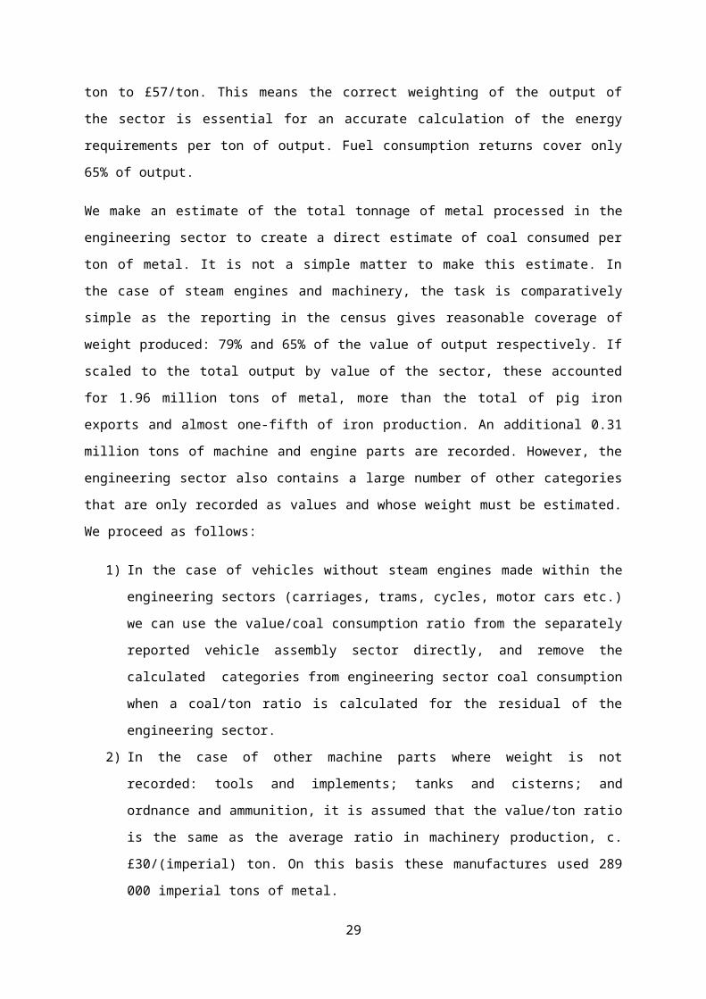
1907: The main problem in calculating coefficients for the products of the engineering sector in this
year is that fuel consumption is given for the sector as a whole, but the weight of output is only given
for sub-sets of particular products. It is clear that the value/weight ratio is not constant across the
sector, and in the products for which we have information varies from £24/(imperial) ton to £57/ton.
This means the correct weighting of the output of the sector is essential for an accurate calculation of
the energy requirements per ton of output. Fuel consumption returns cover only 65% of output.
We make an estimate of the total tonnage of metal processed in the engineering sector to create a
direct estimate of coal consumed per ton of metal. It is not a simple matter to make this estimate. In
the case of steam engines and machinery, the task is comparatively simple as the reporting in the
census gives reasonable coverage of weight produced: 79% and 65% of the value of output
respectively. If scaled to the total output by value of the sector, these accounted for 1.96 million tons
of metal, more than the total of pig iron exports and almost one-fifth of iron production. An
additional 0.31 million tons of machine and engine parts are recorded. However, the engineering
sector also contains a large number of other categories that are only recorded as values and whose
weight must be estimated. We proceed as follows:
1) In the case of vehicles without steam engines made within the engineering sectors (carriages,
trams, cycles, motor cars etc.) we can use the value/coal consumption ratio from the
separately reported vehicle assembly sector directly, and remove the calculated categories
from engineering sector coal consumption when a coal/ton ratio is calculated for the residual
of the engineering sector.
2) In the case of other machine parts where weight is not recorded: tools and implements;
tanks and cisterns; and ordnance and ammunition, it is assumed that the value/ton ratio is
the same as the average ratio in machinery production, c.£30/(imperial) ton. On this basis
these manufactures used 289 000 imperial tons of metal.
3) The amount of copper utilised for electrical cabling and wiring is recorded for 72% of the
output by value, and this is used to produce a total copper consumption estimate of 20 694
imperial tons. Note that iron cabling in telegraphing etc. is recorded separately in a ‘Wire
trade’ sector, not in engineering.
4) A value/weight ratio for electrical machinery can be obtained from the trade statistics, which
as we might expect is very much higher than for most other engineered goods, at £75/ton. It
20

is assumed that other electrical apparatus use metal in the same proportion as those
exported, although the ratio may well be higher. Altogether this electrical engineering sector
used 116 000 imperial tons.
In sum, electrical engineering, ‘other’ iron manufactures and spare parts, and wiring and cabling used
a total of 426 000 tons of metal, against 1.96 million tons for engines and iron and steel machinery,
i.e. engines and non-electrical machines make up 87% of the total. Only a very significant error in
estimate 2) could alter this figure substantially.
Our total estimate of metal consumed in engineering is thus 2.27 million tons, for which 3.51 million
tons of coal were burned (not including adjustments for the coal required to mine coal). This gives us
a sectoral coal/imperial ton ratio of 1.55 tce, not including coal embodied in coal mining. This is very
close to the ratio of 1.53 tce/imperial ton that can also be calculated using an alternative method of
the sectoral coal/value ratio. Translated into GJ/t, the estimated energy requirements within
engineering (including all machinery) are 48.2 GJ/ton and the figure for embodied energy as a whole
is 147.8 GJ/t.
Cotton goods
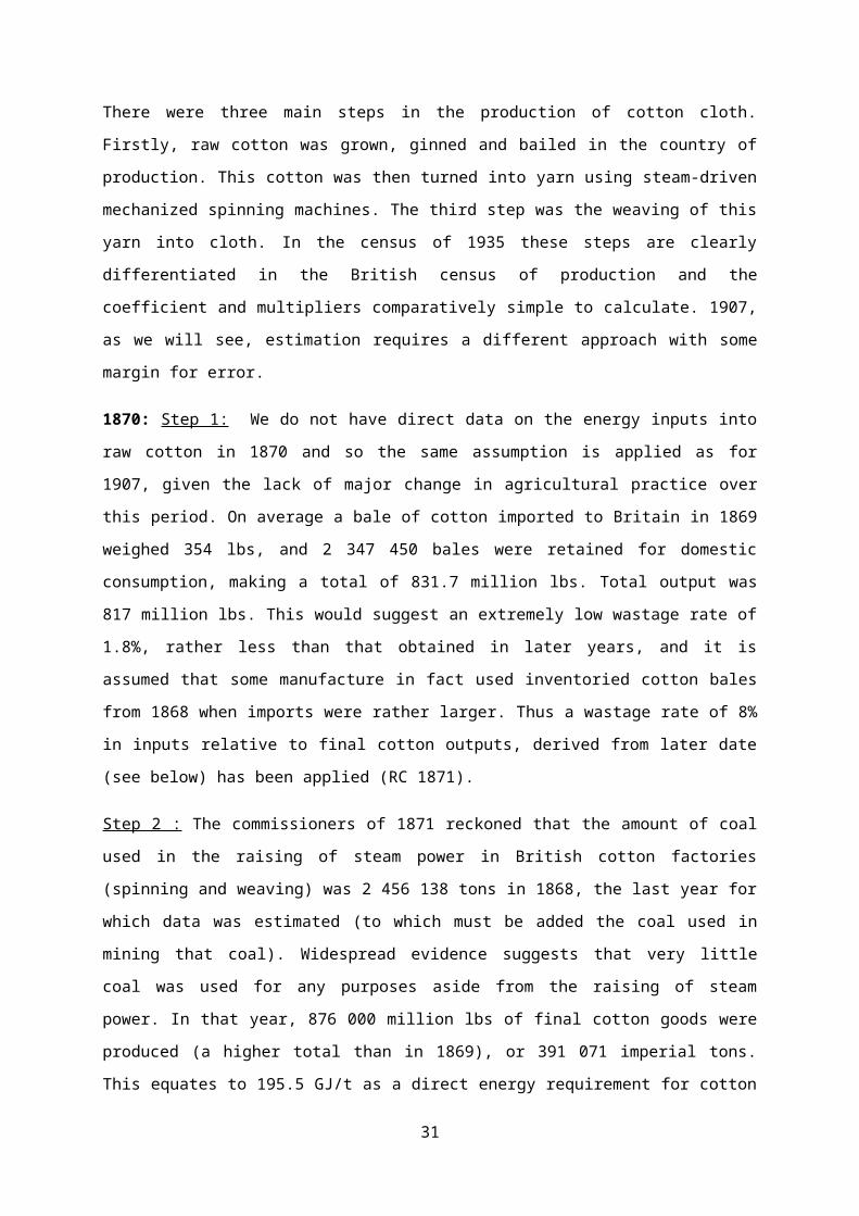
There were three main steps in the production of cotton cloth. Firstly, raw cotton was grown, ginned
and bailed in the country of production. This cotton was then turned into yarn using steam-driven
mechanized spinning machines. The third step was the weaving of this yarn into cloth. In the census
of 1935 these steps are clearly differentiated in the British census of production and the coefficient
and multipliers comparatively simple to calculate. 1907, as we will see, estimation requires a
different approach with some margin for error.
1870: Step 1: We do not have direct data on the energy inputs into raw cotton in 1870 and so the
same assumption is applied as for 1907, given the lack of major change in agricultural practice over
this period. On average a bale of cotton imported to Britain in 1869 weighed 354 lbs, and 2 347 450
bales were retained for domestic consumption, making a total of 831.7 million lbs. Total output was
817 million lbs. This would suggest an extremely low wastage rate of 1.8%, rather less than that
obtained in later years, and it is assumed that some manufacture in fact used inventoried cotton
bales from 1868 when imports were rather larger. Thus a wastage rate of 8% in inputs relative to
final cotton outputs, derived from later date (see below) has been applied (RC 1871).
Step 2 : The commissioners of 1871 reckoned that the amount of coal used in the raising of steam
power in British cotton factories (spinning and weaving) was 2 456 138 tons in 1868, the last year for
21
which data was estimated (to which must be added the coal used in mining that coal). Widespread
evidence suggests that very little coal was used for any purposes aside from the raising of steam
power. In that year, 876 000 million lbs of final cotton goods were produced (a higher total than in
1869), or 391 071 imperial tons. This equates to 195.5 GJ/t as a direct energy requirement for cotton
manufacturing (including the energy embodied in coalmining). The total embodied energy
requirement is thus 245.7 GJ/t.
1907: The quality of data in 1907 made calculations much more complex than did the far more
detailed information in the later censuses of 1924 and 1935. The later census data, where most of
the ratios used below are directly available, is, however, entirely consistent with the processes of
estimation presented here. Unfortunately, in calculating a coefficient for cotton production in 1907
(but not at later dates) we must treat cotton goods as a whole, because fuel inputs recorded in the
census of production are not differentiated between spinning and weaving. There are thus only two
steps in calculating embodied energy inputs.
Step 1: The production of raw cotton, which is drawn from estimates of the use of draught animal
power in American agriculture. Here we calculated the input of draught power per hectare, and then
calculating the average yield of cotton per hectare to assign a value per unit of output. 15 Cotton was
also ginned using steam-driven gins but we have been unable, thus far, to provide a definitive energy
requirement for this process. We estimate that this required 46.5 GJ/t of raw cotton. The coefficient
for producing a ton of raw cotton must then be subject to an adjustment to reflect losses in the
production process; around 6-9% was lost during spinning in 1907 (a figure that declined over time),
and we have used a multiplier of 1.08. This means that the embodied energy from raw cotton
production in each ton of output of cotton goods was 50.2 GJ/t.
Step 2: The energy consumed in manufacturing is then related to the total weight of final cotton
outputs. Firms producing over 81% of net production were accounted for in the returns, and it is
assumed these are representative of the sector as a whole. By far the greater share of this final
output was finished cloth (often called ‘pieces’) of some kind, but some was exported yarn and waste
cotton products (which were recycled for yarn but also used as packing and insulation). As yarn and
waste were subject to one less step than woven cloth, this means the average coefficient for cotton
goods as a whole calculated is somewhat lower than the true coefficient for finished cloth, but
obviously higher than that for yarn by itself.
15 Data was taken from Carter (2006)
22

As 13.4 % of yarn was exported, and 83% of that retained was used for production of woven cotton
pieces, this means the share of yarn production used in woven cloth was (100-13.4)*0.83 = 71.9%.
89% of woven cotton pieces were then exported. That means that of the total weight of cottons
exported was 13.4 + (71.9/0.89) of total production, or 77.4%. Of this, 17.3% was yarn and 82.7%
woven pieces. Thus domestically, woven cloth made up 71.9% of production, but in exports, 82.7%.
As our coefficient is based on the final output of all cotton goods, this difference in composition
means that it will be too low in respect to exports, which contained a larger share of woven cotton
which embodied more energy.
How serious is this compositional error? In 1935, spinning used 62% of the fuel and weaving 38% in
making one ton of woven cotton cloth. This ratio may not, of course, have remained stable over time,
but if we treat it as roughly indicative, then it would suggest that the ratio between the average
coefficient of domestic production, and average coefficient of exports, would have been
(28.1*0.62)+(71.9*1)/(17.3*0.62)+(82.7*1) = 89.3/93.4 = 95.6, or estimate of energy requirements
would be roughly 95.6% of the true energy requirements. Hence the error, for our purposes, is small.
The total tonnage of cotton output was 803 571 imperial tons (the sum of yarn exported plus that
turned into woven or other cotton goods). The direct energy requirements in manufacturing were
169.2 GJ/t, and thus the multiplier for calculating total embodied energy was 219.4 GJ/t.
Total Woollen Goods
The methodological issues here are essentially identical to those for cotton; the inability to
distinguish between energy inputs into yarn only, and into weaving or other processes. An additional
difficulty with wool is that a substantial amount of the material input comes from recycled rags. In
addition, at each stage of wool production, substantial amounts of material are exported. The energy
inputs into the raw wool clip was very low and treated as zero.
1870: The amount of coal consumed in the raising of steam power for the woollen and worsted
industries was calculated by the Royal Commission on Coal independently for England and Scotland,
on the basis of returns of installed horsepower from surveys of 1868, and an estimated consumption
of 8lbs per hp per hour of operation (the returns give rather higher figures than those of the Factory
Returns of 1871 and are likely to be more complete). With coal required in mining that fuel input, the
estimated total coal requirement was 1 143 775 imperial tons in woollen and worsted production.
Average output of woollens for the four years 1864-8 was reckoned to be 241 million lbs, or 107 621
imperial tons. In combination these figures suggest an energy requirement of 311.3 GJ/t. This does
23

not include the use of water power, although by this time it was already relatively marginal as a
power source in Britain and represented a much lower share of primary energy inputs (HMSO 1871) .
1907: The following is based on an input-output table that has been calculated for wool and worsted
production in 1907 from the Census of Production. Points for remark are:
1) It is to be noted that there is a substantial rag recycling which involves sorting in factories,
carbonization of pulverization of rags, and the making of ‘pulled wool’ products such as
shoddy and mungo (rages and waste wool compressed together into a kind of felted
material). Some of this is exported but by far the greater share is used as an input into
woollen yarn manufacture. In fact, for our calculation this only matters because 6% of the
shoddy is exported. This is treated as if it had zero energy inputs. As most of the pulled wool
(207 million lbs) goes into yarn production it is accounted for in the final outputs of the trade
which are related to total fuel consumption.
2) There were very substantial weight losses between the receipt of the imported raw wool
‘clip’, which must be washed, and its further use by the processing industry. Some raw wool
is also exported, and a small amount retained as stock. This phase of processing is treated as
if no fuel is consumed for the purposes of this calculation. We may note that the ratio of coal
to hp suggests that the great majority of coal used in the woollen industries is used to drive
steam engines and not for other purposes such as heating water, space etc.
3) Retained raw wool (amounting to 347 million lbs) was then processed into ‘tops’, and ‘noils’.
For the purposes of the input-output table other waste wool (‘flocks’) that is gathered up at
other parts of the processing and recycled in yarn production is added here as a use of the
raw wool and allocated into the specific ‘flocks’ sub-sector as an input. ‘Tops’ are combed
wool ready for making worsted yarns. ‘Noils’ are essentially a waste product from combing
that can be used in making woollen yarns. A significant amount (35 million lbs) of tops were
exported.
4) The next stage of production is yarn. This differs for woollens and worsteds. Following the
census, we find a c.15% loss is estimated in the spinning and carding process for each
product (doubtless some of this was reintroduced as recycled waste, see point 1 above).
Worsted yarns are made from ‘tops’. 186 million lbs in total were spun, and over 80 million
lbs exported. Woollen yarns are made from the recycled ‘pulled wool’ (see point 1 above),
noils, and flocks, and the remaining washed raw wool. I have estimated that 241 million lbs
of woollen yarn were spun, which is at the lower end of a range estimated in the census, but
that matches best the figures provided when put into the input-output matrix. Very little
woollen yarn was exported, only around 1% of production.
24
5) As the yarn that is not exported is used to weave finished goods (woollen tissues, worsted
tissues, and much smaller quantities of flannel, damasks, carpets, blankets etc.) these figures
allow us to calculate the total amount of final woollen goods. They are the sum of all yarn
that goes into domestic production + exported yarn + exported tops + exported noils. This
comes to 478 million lbs of wool.
6) This figure is used to calculate our per tonne energy requirement, comparing it with all
energy consumed in the woollen and worsted industry (including primary energy for
electricity and embodied coal).
The resulting energy requirement is 262.3 GJ/t of woollen goods.
In terms of individual woollen goods, this coefficient could be significantly in error. Tops, for example,
have only been subject to mechanized combing, not spinning or weaving, while yarn has not been
woven. Woollen tissues (largely made from recycled shoddy but mixed with some uncombed pure
wool and some noils as a by-product of combing) differ in their production processes from worsted
(made with combed tops). If the composition of exports was the same as domestic production this
would not matter. However, while 72% of the weight of wool in finished goods went into products
that had gone through a full range of processing, this is only true of 57.8% of exports (the weight of
exports had to be estimated by using lb/yard ratios calculated from the census; and in the case of
some products such blankets and hosiery where no weight is recorded, assuming this were alike to
carpets and woollen tissues, respectively; shoddy and raw wool is excluded). 12.7% of export weight
is accounted for by ‘tops’ although they accounted for only 7.5% of final woollen products using coal
in their production. For exports the estimate of energy requirements is thus a little too high, but to
an unknown degree. Any effect on our results would however be marginal.
Chemicals
1870: The really significant traded output of the British chemical industry was alkalis (soda ash,
bleaching powder etc.). The main inputs to alkali production were limestone, salt, pyrites, and
saltpetre. Of these, only salt is likely to have had any significant influence on indirect energy
requirements. Use of coal in saltworks is reported in the 1871 Royal Commission report and it was
estimated that salt required about half a ton of coal per ton of salt, that is, or 14-15 GJ/tons in
energetic terms. We take the energy requirements to be 14.9 GJ/t including embodied energy in the
coal from mining.
25
Evidence from firms’ costs suggests that salt inputs to alkali production were around 1.25 tons per
ton of soda ash produced, representing an indirect energy requirement of 18.6 GJ/ton. The report of
the Royal Commission allows us to assess the amount of fuel used per ton of salt input; the ratio is 3-
3.2. If 3.1 tons of coal were used per ton of salt, this implies 3.1*1.25 tons of coal was used per ton of
alkali output, or 3.9 tons (imperial), and a direct energy requirement of 121.1GJ/t (including
embodied energy in the coal). This consistent with the range of direct reports of firms’ coal use per
ton of soda ash reported in Warren (1980).16Combined, these give us a hidden energy requirement of
139.6 GJ/t.
1907: The chemical industry is extremely complicated, and the census itself states that because of
‘the varied and complicated nature of the industry’, where many products are inputs into others, ‘it
has not been possible to frame any close estimate of the value of the products of this industry taken
as a whole and after allowing for the elimination of all duplication.’ Large amounts of chemicals
produced were used as intermediary products within the industry; for example, only about a third of
sulphuric acid, the most substantial product, was retailed by chemical companies. But this does not
mean that the retailed share can be considered final output, because this may have been bought as
an intermediary product by other chemical firms. Equally, some chemical products were made as by-
products outside of the chemical sector itself; oil refineries, coke ovens and gasworks produced tens
of thousands of tons of ammonium sulphate.17 There were also imports, although predominately of
coal tar dyes whose weight was small (around 16 000 tons).18 However, what concerns us is
establishing a rough estimate of the make of the chemical sector itself which can be related to
energy inputs recorded for that sector. Once we have estimated an energy requirement per ton of
output, the question becomes whether the composition of that output of product corresponds with
the structure of exports. The precise flow of intermediary goods within the sector is not important.
Exports were however almost completely dominated by soda compounds (79.6%) and bleaching
powder (15%). This means we must examine the specific structure of alkali production to see to what
degree it might diverge from the energy requirements outlined above. Inputs into soda compounds
were pyrites, saltpetre, salt, limestone, and coal (see above).
Our time period represents an awkward (for us) zone of transition, as the more efficient Solvay
method was replacing the LeBlanc process rapidly after 1900. 1907 probably represents a rather
mixed picture, with the innovators, the firm of Brunner Mond, having about half the market. But by
16
17 See the 1907 census as reported in in the 1924 census in HMSO (1931).
18 Ibid., p.26.
26

1913, their Solvay, ammonia—soda method was completely in the ascendancy (Reader 1970, Haber
1971, Musson 1978).
The limestone input in the Solvay process was about two tons per ton of output, which given the
energy requirements for quarrying, represents around 1.2 GJ/ton of final output. Salt inputs to alkali
production were recorded in the census as around 500 000 tons, whilst output was recorded as 807
000 tons (soda compounds + bleaching powders). This ratio seems to small compared to direct
estimates of manufacturers’ inputs available from the 1870s-1890s, which imply that we should
assign all of the inputs to the chemical sector to alkalis, or 774 000 tons. This produces a coefficient
of inputs to output rather closer to 1 ton per ton, and thus the indirect energy requirement we can
calculate from the saltworks sector was 13.8 GJ/t. The energy costs of pyrite and saltpetre inputs
were very low. Hence indirect energy requirements for soda compounds were probably around 15
GJ/t in the early 20th century for the Leblanc, Solvay, and indeed other processes. 19
Direct fuel requirements in soda compound production are difficult to calculate because it is not
always clear whether data relates to all of the steps within a chemical production process, or only
particular ones. The typical soda production process first saw sulphuric acid produced using
brimstone or pyrites. Sulphuric acid used much less energy than out calculation of requirements for a
generic ton of chemicals: Drössler seems to have reckoned about 7.33 GJ/t for sulphuric acid in
Germany, and Partington a little less for the main but incomplete part of the process (Kreps 1938;
Partington 1918). In 1924, sulphuric acid inputs into soda compounds were only around 0.11 tons per
ton of output, so it is likely that any error in regard to the stage of acid production is marginal in any
case. The acid was applied to common salt to produce the salt-cake, from which hydrochloric acid
was a by-product which then was absorbed by lime to make bleaching powder. Meanwhile the salt
cake was calcined with limestone to produce soda ash (Kreps 1938). However, there was still a range
of different processes to achieve this, so data on the energy requirements of one of these in no way
resolves the question of the average. Best-practice was the Solvay process that according to Ayres
and Warr (2003) had achieved 25 GJ/t by 1913; Partington (1918) gives a figure of 17.8 GJ/t in the
1910s; and put the making of bleaching powder at around bleaching powder 9-15 GJ/t. Earlier
commercial data suggests the Leblanc process by the 1890s still using as a direct energy requirement
around 82 GJ/t from coal, while the Solvay process used 70 GJ/t at its inception in the 1870s and 62
GJ/t in the 1890s (Haber 1958). These figures suggest that Ayres and Warr’s (2003) estimate of 50
GJ/t for the early use of the Solvay process in the USA is either too low or inappropriate for European
comparisons. Even if fuel use had fallen by the rate they suggest, c.50% by 1910, we would still
expect very best practice in the industry to have a direct energy requirement of 35 GJ/t, and a total
19 Estimates from firms of inputs to soda ash production can be found Haber (1958).
27

hidden energy requirement of 50 GJ/t. As it happens this is almost exactly, and perhaps
coincidentally, the same as an estimate we have independently calculated for the chemical sector as
a whole in 1907.
3.3. Embodied energy intensities and sources
Denmark:
Figure 6. Embodied energy intensities of various Danish agricultural products exported or used as
an input to export products 1876 and 1913
Embodied energy
intensities
Energy conten
t
Hidden Energy Requirements
Total Hidden
Fuels and Feed for draught
Feed Lossesa
GJ/t GJ/t GJ/t GJ/t GJ/tDenmark (1876)Used in Exports:Barley 17 13 5 5Butter 502 33 469 82 386Pork and bacon 115 17 98 30 68Beef 69 11 48 10 38Oats 16 10 6 6Wheat Flour 19 13 7 7Oil cake (US, 1909) 22 13 9 9Denmark (1913)
28
Used in Exports:Beer 13 2 11 11Butter 382 33 348 93 255Barley 17 13 5 5Eggs 234 6 228 80 148Pork, Bacon 142 17 126 43 82Beef 56 10 46 9 38Milk, Condensed 41 13 27 27Beetroot 16 16 0.4 0.4Raw potatoes 3 3 0.3 0.3Used for construction:Phosphate Rock (US, 1905) 5 5Chile Nitrate (Chile, 1913) 11 11Superphosphates (US, 1914) 6 6Calcium Nitrate (Norway, 1920) 45 45Oil cakes (US, 1914) 20 13 8Rootcrops to feed (average, 1913) 2 1.3 0.3 0.3Grain as feed (average, 1913) 18 12 6.2 6.2
Note: aFeed Losses correspond to the energy conversion losses which occur in the process of transforming feed for non-working animals into food.
Figure 7. Summary of Embodied energy intensities of some industrial products United Kingdom
GJ/t GJ/t
Final product 1870 1907
Coal 31 31
Pig iron 81 66
Iron and steel goods 177 99
Machinery 148
Cotton goods 246 219
Woollen goods 311 262
Salt 15 14
Chemicals 140 50
Sources
General:
29

Aguilera, E., Guzmán, G. I., Infante-amate, J., García-ruiz, R., Herrera, A., & Villa, I. (2015). Embodied Energy in Agricultural Inputs. Incorporating a historical perspective, 123. Retrieved from http://hdl.handle.net/10234/141278
Bullard W, Penner PS, Pilati DA (1978) Net energy analysis: Handbook for combining process and input-output analysis. Resour energy 1:267–313.
Fluck R (1992) Energy of human labour. In: Energy in agriculture: Energy in farm production, vol 6, Elsevier, Amsterdam, pp 31–43
Krausmann F (2004) Milk, manure, and muscle power. Livestock and the transformation of preindustrial agriculture in Central Europe. Hum Ecol 32:735–772. doi: 10.1007/s10745-004-6834-y
Jensen, E. (1937). Danish agriculture: its economic development. Copenhagen: J.H. Schulz Forlag.
Sorman, A. H., & Giampietro, M. (2013). The energetic metabolism of societies and the degrowth paradigm: Analyzing biophysical constraints and realities. Journal of Cleaner Production, 38, 80–93. https://doi.org/10.1016/j.jclepro.2011.11.059
Stanhill G (1980) The energy cost of protected cropping: a comparison of six systems of tomato production. J Agr Eng Res 25:145–154.
For Danish embodied energy intensities:
Danish figures:
Bøggild B (1901) Maelkeribruget i Danmark 1900, Tidskrift for Landokonomi.
Bøggild B (1914) Maelkeribruget i Danmark 1913, Tidskrift for Landokonomi.
Henriques, S. T., & Sharp, P. (2016). The Danish agricultural revolution in an energy perspective: a case of development with few domestic energy sources. Economic History Review, 69(3), 844–869. https://doi.org/10.1111/ehr.12236
Henriksen OB, Ølgaard A (1960) Danmarks Udenrigshandel 1874-1958. University of Copenhagen, Copenhagen. University of Copenhagen, Copenhagen
Jensen, E. (1937). Danish agriculture: its economic development. Copenhagen: J.H. Schulz Forlag.
Lampe M, Sharp P (2015) Just add milk: A productivity analysis of the revolutionary changes in nineteenth-century Danish dairying. Econ Hist Rev 68:1132–1153. doi: 10.1111/ehr.12093
Lindhard E (1926) Danmarks landbrug 1875-1925. In: Dannfelt H, Lindhard E, Rindell A (eds) Lantbruket i Norden under senast halvsekel 1875-1925. Goteborg Litografiska Aktiebolag, Gothenburg
Raaschov PE (1923) Beretning over Dansk Kvælstofindustris forsøgsvirksomheds, Arbejde i Tidsrummet fra 1 Okt 1918 til 1 Oktober 1921. Ingeniøren 4:37–44.
30
Schroll H (1994) Energy-flow and ecological sustainability in Danish agriculture. Agric Ecosyst Environ 51:301–310. doi: 10.1016/0167-8809(94)90142-2
SD-Statistics Denmark (1913) Statistik aarbog 1913. H.H. Thiels Bogtrykkerie, Copenhagen
SD-Statistics Denmark. (1916a) Produktionsstatistik for aaeret 1913, Statistics Denmark, Copenhagen.
SD-Statistics Denmark. (1916b) Mejeribruget i Danmark i 1914. Statistik Meddelelser, 4, 49, 1.
SD- Statistics Denmark (1917). Danmarks haandværk og industri 1914. Statistisk Tabelværk VA,12.
SD-Statistics Denmark (1960) Energiforsyning 1900-1958, Statistik Undersøgelser 2, Copenhagen.
SD-Statistics Denmark (1968) Agricultural Statistics 1900-1965, vol. 1: agricultural area and harvest and utilization of fertilizers, Statistik Undersøgelser 24, Copenhagen.
SD-Statistics Denmark (1969) Agricultural Statistics 1900-1965, vol. 2: Livestock and Livestock Products and Consumption of Feeding Stuffs, Statistik Undersøgelser 25, Copenhagen.
(1914) Statistik for Danske ProvinsElektricitestvaerker. Odense
Sveistrup P, Willerslev R (1945) Den danske sukkerhandels og sukkerproduktions historie. Institutet for Historie og Samfundsokonomi., Odense
Smil V (2001) Enriching the Earth: Fritz Haber, Carl Bosh and the Transformation of the World Food production. MIT, Massachussets
Statens Kuldfordelingsudvalg (1921) Kulforholdene i Danmark 1914-1920. Copenhagen
Warming K (1923) Om mulighederne for en danske kvaelstofindustri. Ingeniøren 25:309–317.
Foreign inputs:
Carter, S. B., Olmstead, A. L., Sutch, R., Wright, G., & Hains, M. R. (2006). The Historical statistics of the United States: Economic Sectors (Milennium). New York: Cambridge University Press.
OCE-Oficina Central de Estadistica. (1914). Anuario estadistico de la Republica do Chile, vol 7, mineria y metalurgia. Santiago do Chile: Soc. Imp. Y Cit. Universo.
US Bureau of Census Department of Commerce (1917) Abstract of the census of manufactures 1914. Government Printing Office, Washington
Winkel J (1881) Mjeribruget i Danmark i 1880. Copenhagen
For British embodied energy intensities:
Ayres, R. U., Ayres, L. W., & Warr, B. (2003). Exergy, power and work in the US economy, 1900 - 1998. Energy, 28(3), 219–273. https://doi.org/10.1016/S0360-5442(02)00089-0
31

British Iron and Steel Federation. (1949). A simple guide to basic processes in the iron and steel. London.
HMSO- Her Majesty’s Stationery Office (1871) Report of the Commissioners appointed to inquire into the several matters relating to coal in the United Kingdom. Vol. I. General report and twenty-two sub-reports, Appendix E. HMSO, London
HMSO- Her Majesty’s Stationery Office (1913) Final report on the first census of production of the United Kingdom (1907). HMSO, London
HMSO- Her Majesty’s Stationery Office (1931) Final report on the third census of production of the United Kingdom (1924). Vol. IV. The Chemical and allied trades, the leather, rubber and canvas goods trades, the paper, printing & allied trades, and miscellaneous. HMSO, London
Kreps, T. J. (1938). The economics of the sulfuric acid industry. California: Standford University Press.
McCloskey, D. (1973). Economic maturity and entrepreneurial decline. Cambridge, MA: Harvard University Press.
Musson, A. (1978). The growth of British industry. London: Batsford.
Partington, J. R. (1918). The Alkali industry. London.
Reader, W. J. (1970). Imperial Chemical Industries: a history, vol. 1, The forerunners 1870-1926. Oxford: Clarendon.
Warren, K. (1926). Chemical foundations. The alkali industry in Britain to 1926.
Foreign inputs
Carter, S. B., Olmstead, A. L., Sutch, R., Wright, G., & Hains, M. R. (2006). The Historical statistics of the United States: Economic Sectors (Milennium). New York: Cambridge University Press.
Kommerskollegium (1918) Bränsleförbrukningen åren 1913-1917 vid industriella anläggningar,
Kommunikationsanstalter samt allmänna verk och inrättningar. Isaac Marcus Boktryckeri, Stoclholm
32

33