Embed Size (px)
Citation preview

University of South FloridaScholar Commons
Graduate Theses and Dissertations Graduate School
6-24-2016
Statistical Analysis of a Risk Factor in Finance andEnvironmental Models for BelizeSherlene Enriquez-SaveryUniversity of South Florida, [email protected]
Follow this and additional works at: http://scholarcommons.usf.edu/etd
Part of the Teacher Education and Professional Development Commons
This Thesis is brought to you for free and open access by the Graduate School at Scholar Commons. It has been accepted for inclusion in GraduateTheses and Dissertations by an authorized administrator of Scholar Commons. For more information, please contact [email protected].
Scholar Commons CitationEnriquez-Savery, Sherlene, "Statistical Analysis of a Risk Factor in Finance and Environmental Models for Belize" (2016). GraduateTheses and Dissertations.http://scholarcommons.usf.edu/etd/6231

Statistical Analysis of a Risk Factor in Finance and Environmental Models for Belize
by
Sherlene Enriquez Savery
A dissertation submitted in partial fulfillment
of the requirements for the degree of
Doctor of Philosophy
Department of Mathematics and Statistics
College of Arts and Science
University of South Florida
Major Professor: Chris P. Tsokos, Ph.D.
Kandethody Ramachandran, Ph.D.
Lu Lu, Ph.D.
Dan Shen, Ph.D.
Date of Approval:
June 18, 2016
Keywords: Risk, Time Series, Rainfall, Tourism
Copyright © 2016, Sherlene Enriquez Savery

Acknowledgments
I would like to express my deep appreciation to Professor Chris P. Tsokos for his patient advice,
generous support, friendship, and the countless hours of personal time he has spent assisting me
throughout my graduate career. His guidance has fostered an environment that has helped me
complete this work diligently and with greater ease than would have been possible otherwise.
I would also like to express my appreciation to my dearest husband, Laird Savery, my mother,
Constance Mendez and my children, Laird Jr. and Salimah for their patience and understanding
throughout this process, and also for their continuing encouragement. I also thank God almighty
for never leaving my side, for ever being a vital source of strength and for continuing to refuel
my soul in those moments when I have felt despair.

i
Table of Contents
List of Tables .......................................................................................................................... iii
List of Figures ........................................................................................................................... iv
Abstract ..................................................................................................................................... vi
Chapter 1: Importance of the Present Studies; A Review ............................................................. 1
Introduction ..................................................................................................................... 1
Chapter 2: Risk Analysis for Investment ..................................................................................... 5
Introduction ..................................................................................................................... 5
A Review of Current Risk Models ................................................................................... 7
The Capital Asset Pricing Model (CAPM) ........................................................... 7
Conditional CAPM ............................................................................................ 10
Arbitrage Pricing Theory.................................................................................... 14
Fama–French Three-Factor Model ................................................................................. 16
Empirical Testing .......................................................................................................... 19
Testing CAPM ................................................................................................... 19
Testing Conditional CAPM ................................................................................ 21
Testing APT ....................................................................................................... 22
Testing Fama–French Three-Factor Model ......................................................... 23
Conclusion .................................................................................................................... 24
Chapter 3: Proposed Analysis for Estimating Correctly the CAPM Beta.................................... 26
Introduction ................................................................................................................... 26
The Capital Asset Pricing Model (CAPM) ..................................................................... 28
Johnson SU 4-Parameter Probability Distribution .......................................................... 31
Procedure for Estimating the Johnson 4P Probability Distribution ...................... 34
Parameters Estimation ........................................................................................ 37
Analysis of Financial Data ................................................................................. 39
Conclusion .................................................................................................................... 45
Chapter 4: Parametric Statistical Analysis of Belize’s Rainfall .................................................. 47
Introduction ................................................................................................................... 47
Descriptive Statistics ..................................................................................................... 50
Fitting the Wakeby Probability Distribution ................................................................... 55
L- Moment Estimation of Wakeby Probability Distribution ........................................... 58
Result of Fitting The Wakeby Probability Distribution Function .................................... 60
Examining Belize’s Wet and Dry Seasons ..................................................................... 62
Conclusion .................................................................................................................... 65

ii
Chapter 5: Statistical Models for Forecasting Tourists Arrival in Belize .................................... 66
Introduction ................................................................................................................... 66
Structure of Belize’s Economy and Importance of Tourism ........................................... 69
Institutional and Policy Framework ............................................................................... 70
Methodology ................................................................................................................. 73
Holt-Winters Exponential Smoothing ............................................................................ 75
ARIMA Model .............................................................................................................. 78
Comparison of the Forecasting Models .......................................................................... 81
Conclusion .................................................................................................................... 90
Chapter 6: Future Research ....................................................................................................... 91
References ........................................................................................................................................... 93
iii
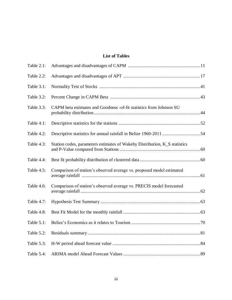
List of Tables
Table 2.1: Advantages and disadvantages of CAPM ............................................................. 11
Table 2.2: Advantages and disadvantages of APT ................................................................. 17
Table 3.1: Normality Test of Stocks ..................................................................................... 41
Table 3.2: Percent Change in CAPM Beta ............................................................................ 43
Table 3.3: CAPM beta estimates and Goodness -of-fit statistics from Johnson SU
probability distribution .......................................................................................... 44
Table 4.1: Descriptive statistics for the stations ..................................................................... 52
Table 4.2: Descriptive statistics for annual rainfall in Belize 1960-2011 ................................ 54
Table 4.3: Station codes, parameters estimates of Wakeby Distribution, K_S statistics
and P-Value computed from Stations .................................................................... 60
Table 4.4: Best fit probability distribution of clustered data ................................................... 60
Table 4.5: Comparison of station’s observed average vs. proposed model estimated
average rainfall .................................................................................................... 61
Table 4.6: Comparison of station’s observed average vs. PRECIS model forecasted
average rainfall ..................................................................................................... 62
Table 4.7: Hypothesis Test Summary .................................................................................... 63
Table 4.8: Best Fit Model for the monthly rainfall ................................................................. 63
Table 5.1: Belize’s Economics as it relates to Tourism .......................................................... 70
Table 5.2: Residuals summary ............................................................................................... 81
Table 5.3: H-W period ahead forecast value .......................................................................... 84
Table 5.4: ARIMA model Ahead Forecast Values ................................................................. 89

iv
List of Figures
Figure 3.1: CAPM Beta Estimates under the Normal and Johnson SU Distribution
Assumption .......................................................................................................... 42
Figure 3.2: Percent Change in CAPM Beta under the Johnson SU vs. the Normal
distribution ........................................................................................................... 43
Figure 4.1: Map of Belize showing the location of the stations ............................................... 48
Figure 4.2: Box Plot of monthly average rainfall in Belize 1960-2011 .................................... 49
Figure 4.3: Histograms of monthly precipitation from sampling stations in Belize .................. 53
Figure 4.4: Box plot for the 15 Stations .................................................................................. 53
Figure 4.5: Box Plot of monthly average rainfall in Belize 1960-2011 .................................... 55
Figure 4.6: Histogram of Monthly Rainfall from sampling stations in Belize
(1964-2011) ……………………………………………………………………57
Figure 5.1: Market Share: Jan – Dec 2015 .............................................................................. 73
Figure 5.2: Plot of tourist’s arrivals in Belize 2000-2013 ........................................................ 74
Figure 5.3: Plot of Tourist arrivals two year forecast .............................................................. 78
Figure 5.4: Plot of tourist’s arrival in between 2000 - 2013 and forecast ................................. 81
Figure 5.5: Forecast from H-W multiplicative model .............................................................. 83
Figure 5.6: Forecasts from Holt Winters model ...................................................................... 84
Figure 5.7: Forecasts from Holt-Winter .................................................................................. 86
Figure 5.8: Holt-Winter residual plot ...................................................................................... 86
Figure 5.9: ACF of the seasonal ............................................................................................. 87
Figure 5.10: Seasonal ARIMA residual plots of tourist arrivals in Belize ................................. 87

v
Figure 5.11: Forecast from ARIMA(1.0,1)(2,1,1)12 ................................................................. 89

vi
Abstract
The objectives of the study are to review and evaluate four basic risk models that are
commonly used in investment science; statistically investigate the risk factor in Capital Asset
Pricing Model (CAPM) that is used to reflect the safety of an investment decision in stocks;
explore the statistical distribution of monthly precipitation in Belize and to forecast tourist
arrivals using statistical time series modelling techniques.
The risk models are the Capital Asset Pricing Model (Sharpe-Linter Version), Capital Asset
Pricing Model (Conditional Version), Arbitrage Pricing Theory, and Fama–French three-factor
model adopted in empirical investigations of asset pricing. The underlying assumptions of using
these models are reviewed, and the statistical procedures to evaluate their robustness are
reviewed.
It will be shown that the present manner of determining this risk factor is quite sensitive
and misleading. We introduce a statistical procedure for obtaining a more robust measure of the
risk factor commonly referred to as CAPM beta.
Changes in the hydrological cycle will generate repercussions in all sectors. It is therefore
imperative that Belize’s water resources be managed in an integrated manner, responding to the
requirements of all sectors. Daily rainfall data have been collected for a period of 51 years
(1960– 2011) from The National Meteorological Service of Belize. The Wakeby distribution
adequately fit the monthly rainfall data producing a suitable model based on the Kolmogorov –
Smirnov test.

vii
Tourism is vitally important to the entire Belize’s economy, contributing 50% of Belize's
gross domestic product in 2015. It is the foremost foreign exchange earner in this small
economy, followed by exports of marine products, citrus, cane sugar, bananas, and garments.
The tourist sector is not without its vulnerabilities and is subject to international economic
vagaries. In order to meet the expected future demands on the industry in terms of service
delivery it is important that the sector understands the significance of forecasting.

1
Chapter 1: Importance of the Present Studies; A Review
This chapter introduces the remainder of the dissertation thesis. We will be presenting its
most basics features, make essential connections between different methodologies that are put
into use, and finally discus the structure of the manuscript.
Introduction
We encounter risks in everything we do, be it, in health, investment, insurance, politics
and defense. The term risk itself is very difficult to pin down precisely. It evokes notions of
uncertainty, randomness, and probability according to Dowd (2005). The random outcome to
which it alludes might be good or bad and we may or may not prefer to focus on the risks
associated with bad events, presumably with a view to try to protect ourselves against them.
Concentrating on the investment aspect, when a portfolio manager gives you a risk value in
making a recommendation, the question that should arise is how good is that value in decision
making? Our finding, is that, the risk is as good as the assumptions their making in the
calculation that convey the risk. This study’s objective is to concentrate on a particular risk
model that we can improved on, to avoid the misleading interpretations and in order to do that,
we identified all the popular models and then we want to dig into these models to see if the
manner in which the risk value is obtain is correct or misleading. It turns out from our results that
some of the risk models are misleading. Before we proceed, a sound understanding of what risk
is and how it is measured is vital. Hence, the first part of chapter 2 is a review of the most
popular models.

2
The notion of risk in its broadest sense therefore has many facets, and there is no single
definition of risk that can be completely satisfactory in every situation (Dowd 2007). However,
for our purpose here, a reasonable definition is to consider it as the likelihood that we will
receive a return on an investment that is different from the return we expected to make.
The normality factor is of concern to us, because to assume normality in the returns
implies symmetry and there is no symmetry in returns. In fact, there is skewness to the left or
right. By making a normal symmetry, the assumption will give a risk factor that is misleading.
The quadratic aspect we are questioning is whether it is the best mathematical characterization or
there should be another one? These are the two aspects we are concern with and we are
investigating them further.
Chapter 3 focuses on the measure of risk that is commonly used in investment namely
CAPM and investigates the underlying assumptions. Historically, most investors included as part
of their management strategy a risk measure that is based on historical factors. The common risk
measure is the risk associated with the Capital Asset Pricing Model. The CAPM model however
is driven by a set of assumptions; one of which is the normality assumption of the returns.
Natural phenomena often produce departures from normality and many recent findings suggest
that the most commonly used estimation methods exhibit varying degrees of non-robustness to
certain violations of the assumption of normality. In practice, it is not customary to get normal
data in many real- world applications, researchers are uncertain about the true nature of the
distribution of the errors and a naïve application of the normal distribution can give the user the
wrong impression that he or she has obtained a useful inferential result. This can lead to
misleading information later being passed on to financial advisors and later to their clients with
regards to investment options. Chapter 3 continues with the introduction of a statistical

3
procedure for obtaining a more robust measure of risk premium beta. This process included the
best justification of the selection process of the probability distribution that drives the estimate of
the CAPM beta. Our research findings indicated that the distribution of beta is not normal but
rather a Johnson 4p probability distribution.
The influence of rainfall on water quality, agriculture and tourism among others cannot
be over emphasized. Because agriculture and tourism are the largest income earners for Belize, it
is vital that we understand our rainfall system and possess the ability to model and forecast the
rainfall, this gives added value to any major investment or planning. In Chapter 4, we focus on
the parametric statistical analysis of Belize’s rainfall. The primary goal of this chapter is to
analyze actual precipitation data collected in fifteen meteorological stations in Belize. There are
other stations but because of data length, we chose only fifteen. We first identify the probability
density function (PDF) that best characterizes the behavior, the Wakeby distribution for the
entire data and then separated the data by the two seasons in Belize namely the wet and dry
season. We conducted a hypothesis testing to determine if there is a distinction between the two
seasons. We then transformed the data using a Box Cox transformation and then do a cluster
analysis on the 15 weather stations.
The determination of the best fit distribution to represent the rainfall process in stations of
Belize is discussed in this paper. An extensive search comparing several distribution such as
Wakeby , lognormal, gamma, Weibull ,Generalized Pareto, Dugan and many other distributions
have been used on the monthly average rainfall data from 1960 to 2011. The selection of the
best fit distribution is done by examining the minimum error produced by the Kolmogorov
Smirnov (KS) goodness of fit test. Based on the results of KS goodness of fit test, Wakeby

4
distribution is the most suitable to describe the rainfall patterns in the stations of Belize as the
error produced is the minimum.
In Chapter 5, we did times series analysis on Belize’s tourist arrival data with the
objective of identifying the best forecasting model. First we test the data for stationarity,
meaning that the mean and variance does not change over time and that the process does not
have a trend. The two forecasting procedures that we utilize are the Holt-Winters exponential
smoothing and Seasonal ARIMA model. Both of these models appear to fit the data well. In
further analysis of the residuals, we conclude that the Holt Winter is the optimal forecasting
model based on the data used in the study. Although our data set was specific, the same
methodology can be applied to similar time series data.
Exponential smoothing and ARIMA models are the two most widely-used approaches to
time series forecasting, and provide complementary approaches to the problem. While exponen-
tial smoothing models were based on a description of trend and seasonality in the data, ARIMA
models aim to describe the autocorrelations in the data
The dissertation concludes with Chapter 6, where possible future directions are explained
along with future consideration with regards to the work already presented.

5
Chapter 2: Risk Analysis for Investment
Introduction
Risk is a part of investing and a sound understanding of what risk is and how it is measures
is vital to investment. We start our discussion by defining risk. Webster’s dictionary defines risk
as “exposing to danger or hazard”. Thus, risk is perceived, by Webster, almost entirely in
negative terms. In finance, our definition of risk is both different and broader. Risk, as we see it,
refers to the likelihood that we will receive a return on an investment that is different from the
return we expected to make. Thus, risk includes not only the bad outcomes, i.e., returns that are
lower than expected, but also good outcomes, i.e., returns that are higher than expected. In fact,
we can refer to the former as downside risk and the latter is upside risk; and we consider both
when measuring risk.
The foundations for the development of asset pricing models were laid by Markowitz
(1952) and Tobin (1958). Early theories suggested that the risk of an individual security is the
standard deviation of its returns – a measure of return volatility. Thus, the larger the standard
deviation of security returns, the greater the risk. An investor’s main concern, however, is the
risk of his/her total wealth made up of a collection of securities, the portfolio. Markowitz (1952)
observed that (i) when two risky assets are combined, their standard deviations are additive only
in the case that the two assets are perfectly positively correlated and (ii) when a portfolio of risky
assets is formed, the standard deviation risk of the portfolio is less than the sum of the standard
deviations of its constituents. Markowitz was the first to develop a specific measure of portfolio
risk and to derive the expected return and risk of a portfolio. The Markowitz model generates the

6
efficient frontier of portfolios and the investors are expected to select a portfolio, which is most
appropriate for them, from the efficient set of portfolios made available. Tobin (1958) suggested
a course of action to identify the appropriate portfolios among the efficient set.
The computation of risk reduction as proposed by Markowitz is tedious. Sharpe (1964)
developed a computationally efficient method, the single index model, where the return on an
individual security is related to the return on a common index. The common index may be any
variable thought to be the dominant influence on stock returns and need not be a stock index
(Jones, 1991). The single index model can be extended to portfolios as well. This is possible
because the expected return on a portfolio is a weighted average of the expected returns on
individual securities.
When analyzing the risk of an individual security; however, the individual security risk
must be considered in relation to other securities in the portfolio. In particular, the risk of an
individual security must be measured in terms of the extent to which it adds risk to the investor’s
portfolio. Thus, a security’s contribution to the portfolio risk is different from the risk of the
individual security. Investors face two kinds of risks, namely, diversifiable (unsystematic) and
non-diversifiable (systematic). Unsystematic risk is the component of the portfolio risk that can
be eliminated by increasing the portfolio size, the reason being that risks that are specific to an
individual security such as business or financial risk can be eliminated by constructing a well-
diversified portfolio. Systematic risk is associated with overall movements in the general market
or economy and therefore is often referred to as the market risk. The market risk is the
component of the total risk that cannot be eliminated through portfolio diversification.

7
The main objective of this chapter is to review the conceptual idea behind asset pricing
models and to discuss the testing and evaluation methods. This chapter is organized as follows.
Section 2 discusses the four commonly used risk models. These risk models are the Capital Asset
Pricing Model (Sharpe-Linter Version), Capital Asset Pricing Model (Conditional Version),
Arbitrage Pricing Theory and a Multifactor model adopted in empirical investigations of asset
pricing. Section 3 discusses the empirical findings regarding the four models. The final section
concludes the chapter. In what follow we shall address very popular investment strategies.
Relevant information on the mission of the present study can be found in Fama and French
(1996), Fama and French (1996), Connor and Sehgal (2001), Chawarit (1996), Chanthirakul
(1998), Fama and French (1992), Ross (1976), Sharpe (1964), Lintner (1965) , Mossin (1966),
Brigham and Ehrhardt ( 2005).
A Review of Current Risk Models
In what follows, we shall address commonly used risk models, the Capital Asset Pricing
Model (Sharpe-Linter Version), Capital Asset Pricing Model (Conditional Version), Arbitrage
Pricing Theory and a Multifactor model which are very popular in investment strategies.
The Capital Asset Pricing Model (CAPM)
Investors who buy assets expect to earn returns over the time horizon that they hold the
asset. Their actual returns over this holding period may be very different from the expected
returns and it is this difference between actual and expected returns that is source of risk. The
risk and return model that has been in use the longest and is still the standard in most real world
analyses is the capital asset pricing model (CAPM). The CAPM conveys the notion that
securities are priced so that the expected returns will compensate investors for the expected risks.

8
There are two fundamental relationships: the capital market line (CML) and the security market
line (SML). These two models are the building blocks for deriving the CAPM.
The CML specifies the return an individual investor expects to receive on a portfolio.
This is a linear relationship between risk and return on efficient portfolios that can be
written as:
𝐸(𝑅𝑝) = 𝑟𝑓 + 𝜎𝑝 (
𝐸(𝑅𝑚) − 𝑟𝑓𝜎𝑚
) (2.1)
where 𝑅𝑝 is portfolio return, 𝑟𝑓 risk-free asset return, Rm market portfolio return, 𝜎𝑝 and standard
deviation of portfolio returns and 𝜎𝑚 is standard deviation of market portfolio returns.
According to Equation 2.1, the expected return on a portfolio can be thought of as the
sum of the return for delaying consumption and a premium for bearing the risk inherent in the
portfolio. The CML is valid only for efficient portfolios and expresses investors’ behavior
regarding the market portfolio and their own investment portfolios.
The Security market line (SML) expresses the return an individual investor can expect in
terms of a risk-free rate and the relative risk of a security or portfolio. The SML with respect to
security i can be written as:
𝐸(𝑅𝑖) = 𝑟𝑓 + 𝛽𝑖𝑚(𝐸(𝑅𝑚) − 𝑟𝑓) (2-2)
where

9
𝛽𝑖𝑚 =
𝜎𝑖𝑚𝜎𝑚2
=𝑐𝑜𝑣(𝑅𝑖 , 𝑅𝑚)
𝜎𝑚2
(2-3)
and 𝜎𝑖𝑚 the covariance between security return, 𝑅𝑖 , and market portfolio return. The
𝛽𝑖𝑚 can be interpreted as the amount of non-diversifiable risk inherent in the security relative to
the risk of the market portfolio. Equation (2.2) is the Sharpe–Lintner version of the CAPM. The
set of assumptions sufficient to derive the CAPM version of (Equation 2.2) are the following:
the investor’s utility functions are either quadratic or normal,
all diversifiable risks are eliminated, and
the market portfolio and the risk-free asset dominate the opportunity set of risky assets.
The SML is applicable to portfolios as well. Therefore, SML can be used in portfolio analysis to
test whether securities are fairly priced, or not.
The three assumptions above can be further broken down into eight assumptions for the CAPM,
namely:
1. Investors are rational and risk averse. They pursue single-mindedly the maximization of
the expected utility of their end of period wealth. Implication: The model includes the
single time horizon for all investors.
2. The markets are perfect, thus taxes, inflation, transaction costs, and short selling
restrictions are not taken into account.
3. Investors can borrow and lend unlimited amounts at the risk-free rate.
4. All assets are infinitely divisible and perfectly liquid.
5. Investors have homogenous expectations about asset returns. In other words, all
investors agree about mean and variance as the only system of market assessment, thus

10
everyone perceives identical opportunity. The information is costless, and all investors
receive the same information simultaneously.
6. Asset returns conform to the normal distribution.
7. The markets are in equilibrium, and no individual can affect the price of a security.
8. The total number of assets on the market and their quantities are fixed within the
defined time frame.
Once you accept the assumptions that lead to all investors holding the market portfolio and
measure the risk of an asset with beta, the return you can expect to make can be written as a
function of the risk-free rate and the beta of that asset. Table 2-1 outlines some advantages and
disadvantages of using CAPM.
Conditional CAPM
One of the commonly made assumptions is that the betas of the assets remain constant over
time. However, this is not a particularly reasonable assumption since the relative risk of a firm's
cash flow is likely to vary over the business cycle. Hence, betas and expected returns will in
general depend on the nature of the information available at any given point in time and vary
over time. Ravi Jagannathan and Zhenyu Wang (1996) assumed that the expected return on an
asset based on the information available at any given point in time is linear in its conditional
beta, and introduced the idea of the Conditional CAPM.
We use the subscript t to indicate the relevant time period. For example, Rit denotes the
gross (one plus the rate of) return on asset i in period t, and Rmt, the gross return on the aggregate
wealth portfolio of all assets in the economy in period t. We refer to Rmt, as the market return.
Let It-1 denote the common information set of the investors at the end of period t - 1. In this paper

11
Table 2.1: Advantages and disadvantages of CAPM
Advantages of CAPM Disadvantages of CAPM
1. Market portfolio includes all the risky assets
including human capital while the proxy just
contains the subset of all assets
2. It has given a measure of risk, market beta,
interpreted as market sensitivity
3. The popularity and Attractiveness of CAPM
is its potential testability
4. If empirically true, it has a wide ranging implication in capital budgeting, cost benefit
analysis, portfolio selection and development
of investment strategies
5. CAPM durability is due to the fact that it
explains return common variability in terms
of a single factor, which generates return for
each individual asset via some linear
functional relationship
6. It considers only systematic risk, reflecting a reality in which most investors have
diversified portfolios from which
unsystematic risk has been essentially
eliminated
7. It generates a theoretically-derived
relationship between required return and
systematic risk which has been subject to
frequent empirical research and testing.
8. It is generally seen as a much better method of
calculating the cost of equity than the dividend growth model (DGM) in that it
explicitly takes into account a company’s
level of systematic risk relative to the stock
market as a whole.
9. It is clearly superior to the WACC in
providing discount rates for use in investment
appraisal.
1. Inability to observe the true market portfolio
2. Liable to Type1 and Type11 errors
3. In order to use the CAPM, values need to be assigned
to the risk-free rate of return, the return on the market,
or the equity risk premium (ERP), and the equity beta.
4. The yield on short-term Government debt, which is
used as a substitute for the risk-free rate of return, is
not fixed but changes on a daily basis according to
economic circumstances. A short-term average value can be used in order to smooth out this volatility.
5. Finding a value for the ERP is more difficult.
6. Beta values are now calculated and published regularly
for all stock exchange-listed companies. The problem
here is that uncertainty arises in the value of the
expected return because the value of beta is not
constant, but changes over time.
7. One disadvantage in using the CAPM in investment appraisal is that the assumption of a single-period time
horizon is at odds with the multi-period nature of
investment appraisal. While CAPM variables can be
assumed constant in successive future periods,
experience indicates that this is not true in reality.

12
we assume all the time series in this paper are covariance stationary and all the conditional and
unconditional moments that we use exist.
Risk-averse rational investors living in a dynamic economy will typically anticipate and
hedge against the possibility that investment opportunities in the future may change adversely.
Because of this hedging need that arises in a dynamic economy, the conditionally expected
return on an asset will typically be jointly linear in the conditional market beta and hedge
portfolio beta. However, employing Merton (1980) findings, we will assume that the hedging
motives are not sufficiently important, and hence the CAPM will hold in a conditional sense as
given below.
For each asset i and in each period t,
𝐸(𝑅𝑖|𝐼𝑡−1) = 𝛾0𝑡−1 + 𝛾1𝑡−1 𝛽𝑖𝑡−1 (2.4)
Where 𝛽𝑖𝑡−1 is the conditional beta of asset i defined as,
𝛽𝑖𝑡−1 =
𝑐𝑜𝑣(𝑅𝑖𝑡 , 𝑅𝑚𝑡|𝐼𝑡−1)
𝑉𝑎𝑟(𝑅𝑚𝑡|𝐼𝑡−1)
(2.5)
γ0t−1, is the conditional expected return on a "zero-beta" portfolio, and 𝛾1𝑡−1, is the conditional
market risk premium.
Since our aim is to explain the cross-sectional variations in the unconditional expected
return on different assets, we take the unconditional expectation of both sides of equation (2) to
get
𝐸(𝑅𝑖𝑡) = 𝛾0 + 𝛾1 �̅�𝑖 + 𝑐𝑜𝑣(𝛾1𝑡−1 , 𝛽𝑖𝑡−1 ), (2.6)
where

13
𝛾0 = 𝐸(𝛾0𝑡−1) , 𝛾1 = 𝐸(𝛾1𝑡−1) 𝑎𝑛𝑑 �̅�𝑖 = 𝐸(𝛽𝑖𝑡−1) .
Here, 𝛾1, is the expected market risk premium, and �̅�𝑖 is the expected beta. If the covariance
between the conditional beta of asset i and the conditional market risk premium is zero (or a
linear function of the expected beta) for every arbitrarily chosen asset i, then equation (4)
resembles the static CAPM, i.e., the expected return is a linear function of the expected beta.
Jagannathan and Wang (1996) argued that the two assumptions of Fama and French
(1992) are not reasonable. Relaxing the first assumption naturally leads them to examine the
conditional CAPM. They demonstrated that the empirical support for the conditional CAPM
specification is rather strong. When betas and expected returns are allowed to vary over time by
assuming that the CAPM holds period by period, the size effects and the statistical rejections of
the model specifications become much weaker. When a proxy for the return on human capital is
also included in measuring the return on aggregate wealth, the pricing errors of the model are not
significant at conventional levels. More importantly, firm size does not have any additional
explanatory power.
The conditional CAPM is very different from what is commonly understood as the
CAPM, and resembles the multi-factor model of Ross (1976). The model evaluated has three
betas, whereas the standard CAPM has only one beta. Jagannathan and Wang(1996) chose this
model because (i) the use of a better proxy for the return on the market portfolio results in a two-
beta model in place of the classical one-beta model, and (ii) when the CAPM holds in a
conditional sense, unconditional expected returns will be linear in the unconditional beta as well
as a measure of beta-instability over time. When the CAPM holds conditionally, we need more
than the unconditional beta calculated by using the value-weighted stock index to explain the
cross-section of unconditional expected returns.
14
Additional relevant information can be found in: Fischer, Jensen, and Scholes (1972),
Fama, Eugene F. (1968) , Fama and French (1992), French, Craig W. (2003) , French, Craig W.
(2002), Lintner, John (1965). Markowitz, Harry M. (1999) , Mehrling, Perry (2005), Mossin,
Jan. (1966) Ross, Stephen A. (1977). , Trey nor, Jack L. (1962), Treynor, Jack L. (1961) , Tobin,
James (1958) and Stone, Bernell K. (1970), Banz (1981), Reinganum (1981), Gibbons (1982),
Basu (1983), Chan, Chen, and Hsieh
(19851, Shanken (19851, and Bhandari (1988), Hansen and Jagannathan (1994) , Hansen and
Singleton (1982), Connor and Korajczyk (1988a and 1988131, Lehmann and Modest (1988), and
Hansen and Jagannathan (1991 and 1994), Jegadeesh (1992), Dybvig, P. H., and J. E. Ingersoll,
Jr., 1982, Black, Fischer, Michael C. Jensen, and Myron Scholes, 1972, Bollerslev, Tim, Robert
F. Engle, and Jeffrey M. Wooldridge, (1988), Zhou, Guofu, (1994) for additional information on
Condtional CAPM.
Arbitrage Pricing Theory
The Arbitrage Pricing Theory (APT) is a very detailed pricing method. The APT is based
on five different economic factors. The factors are: business cycle, time horizon, confidence,
inflation and market timing risk. The advantage of using the APT in portfolio selection and
portfolio risk management is that the model makes the fundamental sources of risk explicit. In
this method these factors are related to the expected return of risky investments. By using these
macroeconomic variables it provides a way to estimate the risk premium for every individual
variable. Why is that important to an investor? For some investors some risk criteria or
variables are more important than others.
To understand the arbitrage pricing model, we need to begin with a definition of arbitrage.
The basic idea is a simple one. Two portfolios or assets with the same exposure to market risk

15
should be priced to earn exactly the same expected returns. If they are not, you could buy the less
expensive portfolio, sell the more expensive portfolio, have no risk exposure and earn a return
that exceeds the riskless rate. This is arbitrage. If you assume that arbitrage is not possible and
that investors are diversified, you can show that the expected return on an investment should be a
function of its exposure to market risk. While this statement mirrors what was stated in the
capital asset pricing model, the arbitrage pricing model does not make the restrictive assumptions
about transactions costs and private information that lead to the conclusion that one beta can
capture an investment’s entire exposure to market risk. Instead, in the arbitrage pricing model,
you can have multiples sources of market risk and different exposures to each (betas). The model
assumes that the return to the ith
security, Rit , is generated by a multi- index model:
𝑅𝑖𝑡 = 𝑎𝑖 + 𝛽𝑖1(𝐹1𝑡) + ⋯+ 𝛽𝑖𝐽(𝐹𝐽𝑡) + 휀𝑖𝑡 ; 𝑖 = 1,2,…𝑁, (2.7)
Where the Fjt are factors (j=1,2,…,J); the 𝛽𝑖𝐽 are factor loading or sensitivities and 휀𝑖 is a
random variable with E(휀𝑖)=0, E(휀𝑖2)=𝜎𝑖
2, E(휀𝑖휀𝑘)=0 for 𝑖 ≠ 𝑗 and 𝑐𝑜𝑣(휀𝑖 , 𝐹𝑗) = 0 for all i and j.
The focus of the APT is on the expected return 𝐸(𝑅𝑖𝑡). Assuming:
1. There are no arbitrage possibilities
2. The law of large number,
the model implies the following relationship between the expected return to asset and the factor
loadings(sensitivities)
𝐸(𝑅𝑖𝑡) = 𝛼0 + 𝛼1𝑏𝑖1 +⋯+ 𝛼𝐽𝑏𝑖𝐽 + 휀𝑖𝑡 (2.8)
Where 𝛼0 usually equals the risk-free rate of return and 𝛼𝐽 has the interpretation of the expected
return to a portfolio (risk price) with unit sensitivity to factor j and zero sensitivity to all other
factors.

16
The practical questions then become knowing how many factors there are that determine
expected returns and what the betas for each investment are against these factors. The arbitrage
model estimates both by examining historical data on stock returns for common patterns (since
market risk affects most stocks) and estimating each stock’s exposure to these patterns in a
process called factor analysis. A factor analysis provides two output measures:
1. It specifies the number of common factors that affected the historical return data
2. It measures the beta of each investment relative to each of the common factors and
provides an estimate of the actual risk premium earned by each factor.
The factor analysis does not, however, identify the factors in economic terms – the factors
remain factor 1, factor 2 etc. In summary, in the arbitrage pricing model, the market risk is
measured relative to multiple unspecified macroeconomic variables, with the sensitivity of the
investment relative to each factor being measured by a beta. The number of factors, the factor
betas and factor risk premiums can all be estimated using the factor analysis. Table 2.1 outlines
some advantages and disadvantages of APT.
Fama–French Three-Factor Model
The Factor Model expands on the capital asset pricing model (CAPM) by adding size and
value factors in addition to the market risk factor in CAPM. This model considers the fact that
value and small cap stocks outperform markets on a regular basis. By including these two
additional factors, the model adjusts for the outperformance tendency, which is thought to make
it a better tool for evaluating manager performance.

17
Table 2.2: Advantages and Disadvantages of APT
Advantages of APT Disadvantages of APT
1. Underlying assumption is that the
return generating process is
stationary
2. APT operates under relative
weaker assumptions
3. Emphasis on multiple systematic
risk
4. It appears to better explain
investment results and more
efficiently controls portfolio risks
5. APT models allow for priced
factors that are orthogonal to the
market return and do not require
that all investors are mean–
variance optimizers, as in the
CAPM
6. The APT demands that investors
perceive the risk sources, and that
they can reasonably estimate factor
sensitivities.
1. The number of institutional
investors actually using APT is
small
2. The arbitrage pricing model's
failure to identify the factors
specifically in the model may be a
statistical strength, but it is an
intuitive weakness
3. Even professionals and academics
can't agree on the identity of the
risk factors, and the more betas you
have to estimate, the more
statistical noise you must live with.
Previous work shows that average returns on common stocks are related to firm
characteristics like size, earnings/price, cash flow/price, book-to-market equity, past sales
growth, long-term past return, and short-term past return. Because these patterns in average
returns apparently are not explained by the CAPM, they are called anomalies. Eugene Fama and
Kenneth French find that, except for the continuation of short-term returns, the anomalies largely
disappear in a three-factor model. Their results are consistent with rational ICAPM or APT.
CAPM uses a single factor, beta, to compare the excess returns of a portfolio with the excess
returns of the market as a whole. But it oversimplifies the complex market. Fama and French
started with the observation that two classes of stocks have tended to do better than the market as
a whole: (i) small caps and (ii) stocks with a high book-to-market ratio (BM, customarily called

18
value stocks, and different from growth stocks). They then added two factors to CAPM to reflect
a portfolio's exposure to these two classes:
𝐸(𝑟𝑝) = 𝑟𝑓 + 𝛽𝑡𝑚(𝐸(𝑟𝑚) − 𝑟𝑓) + 𝛽𝑡,𝑆𝑀𝐵(𝑆𝑀𝐵) + 𝛽𝑡,𝐻𝑀𝐿(𝐻𝑀𝐿) + 휀𝑝 (2-9)
Here 𝑟𝑝 is the portfolio's rate of return, rf is the risk-free return rate, and rm is the return of the
whole stock market. The "three factor" β is analogous to the classical β but not equal to it, since
there are now two additional factors to do some of the work. SMB stands for "small (market
capitalization) minus big" and HML for "high (book-to-price ratio) minus low"; they measure the
historic excess returns of small caps over big caps and of value stocks over growth stocks. These
factors are calculated with combinations of portfolios composed by ranked stocks and available
historical market data.
Fama and French (1993) find that the three-factor risk-return relation is a good model for the
returns on portfolios formed on size and book-to-market equity. They found that the three factor
model also explains the strong patterns in returns observed when portfolios are formed on
earnings/price, cash flow/price, and sales growth, variables recommended by Lakonishok,
Shleifer, and Vishny (1994) and others. The three-factor risk-return relation also captures the
reversal of long-term returns documented by DeBondt and Thaler (1985). Thus, portfolios
formed on E/P, C/P, sales growth, and long-term past returns do not uncover dimensions of risk
and expected return beyond those required to explain the returns on portfolios formed on size
and BE/ME. Fama and French (1994) extend their conclusion to industries. The three-factor risk-
return relation (Equation 2.9) is, however, just a model. It surely does not explain expected
returns on all securities and portfolios. We find that (1) cannot explain the continuation of short-
term returns documented by Jegadeesh and Titman (1993) and Asness (1994).

19
Empirical Testing
The current approaches of testing and calculating the risk factor on investment returns are
sensitive to the assumption of the symmetry. The accuracy and robustness of the models in
discussed above is still yet to be answered. As part of the review process we examined the
different methods in which the models of interest are tested.
Testing CAPM
Another possible problem in many early tests of CAPM has arisen due to it being a single
period model. Most tests have used time series regression, which is appropriate, if the risk
premia and betas are stationary, which is unlikely to be true.
Several researches have focused on the validity of CAPM and the findings from earlier to even
more recent ones appear to be mixed. In order to test the validity of the CAPM researchers,
always test the SML given in (Equation 2.10). The CAPM is a single-period ex-ante model.
However, since the ex-ante returns are unobservable, researchers rely on realized returns. So the
empirical question arises: Do the past security returns conform to the CAPM? The beta in such
an investigation is usually obtained by estimating the security characteristic line (SCL) that
relates the excess return on security i to the excess return on some efficient market index at time
t. The ex post SCL can be written as:
𝑅𝑖𝑡 − 𝑟𝑓𝑡 = 𝛼𝑖 + 𝑏𝑖𝑚(𝑅𝑚𝑡 − 𝑟𝑓𝑡) + 휀𝑖𝑡 (2.10)
where 𝛼𝑖 is the constant return earned in each period and 𝑏𝑖𝑚 is an estimate of 𝛽𝑖𝑚 in the SML
(Jensen, 1968). The estimated 𝛽𝑖𝑚 is then used as the explanatory variable in the following cross-
sectional equation:

20
𝑅𝑖𝑡 − 𝑟𝑓𝑡 = 𝛾0 + 𝛾1𝑏𝑖𝑚 + 𝛿𝑖𝑡 (2.11)
to test for a positive risk return trade-off. The coefficient 𝛾0 is the expected return of a zero beta
portfolios, expected to be the same as the risk-free rate, and 𝛾1 is the market price of risk (market
risk premium), which is significantly different from zero and positive in order to support the
validity of the CAPM. When testing the CAPM using (4) and (5), we are actually testing the
following issues: (i) bim’s are true estimates of historical 𝛽𝑖𝑚’s, (ii) the market portfolio used in
empirical studies is the appropriate proxy for the efficient market portfolio for measuring
historical risk premium and lastly whether the CAPM specifications are correct. Other
methodology have been used for estimating the market model like Lagrange Multiplier,
Maximum likelihood ratio test and Hotelling T2 statistics , they all reject CAPM.
The mixed empirical findings on the return–beta relationship prompted a number of responses:
The single-factor CAPM is rejected when the portfolio used as a market proxy is
inefficient (See [2], for example, Roll, 1977; Ross, 1977). Even very small deviations
from efficiency can produce an insignificant relationship between risks and expected
returns (Roll and Ross, 1994; Kandel and Stambaugh, 1995).
Kothari et al. (1995) highlighted the survivorship bias in the data used to test the
validity of the asset pricing model specifications.
Beta is unstable over time (see, for example, Bos and Newbold, 1984); Faff et al.,
1992; Brooks et al., 1994; Faff and Brooks, 1998).
There are several model specification issues: For example, (i) Kim (1995) and
Amihud et al. (1993) argued that errors-in-the-variables problem impact on the

21
empirical research, (ii) Kan and Zhang (1999) focused on a time-varying risk premium,
(iii) Jagannathan and Wang (1996) showed that specifying a broader market portfolio can
affect the results and (iv) Clare et al. (1998) argued that failing to take into account
possible correlations between idiosyncratic returns may have an impact on the results.
Testing Conditional CAPM
The test of CCAPM becomes very difficult due to the problem of observing expected
market return. To overcome the difficulties Tim Bolerslev (1988) ,Hall(1989) and Ng(1991)
suggested to assume market price risk to be constant and hence requires a functional
specification of variance and covariance structure. In earlier research works the presence of time
varying moments in return distribution has been in the form of clustering large shocks of
dependent variables and thereby exhibiting a large positive or negative value of the error term
[Mandelbrot (1963) and Fama (1965)]. A formal specification was ultimately proposed by Engle
(1982) in the form of Autoregressive Conditional Heteroscedastic (ARCH) process. Some of the
latter studies have attempted to improve upon Engle’s ARCH specification [Engle and
Bollerslev(1986)]. The approaches which are helpful in specifying functional form of error term
in the test of CCAPM include the approaches given by Engle and Bollerslev (1986); Bollerslev
et al. (1992) and Ng et al. (1992) in case of family of ARCH model.
The implicit assumption of Engle ARCH and Bollerslev GARCH is that return
distribution characterized with time variation only in variance. But the evidence from various
studies has shown time variation in both mean and variance of return distribution [Domowitz and
Hakkins (1985)]. Incorporating this idea Engle (1987) has proposed the ARCH-M to account for
time variation in both mean and variance

22
Lewellen and Nagel (2006) test the conditional CAPM by directly estimating conditional
alphas and betas using short window regressions. That is, rather than estimate (Equation 2.2)
once using the full times series of returns, they estimated it separately every, say, quarter using
daily or weekly returns. The result is a direct estimate of each quarter‘s conditional alpha and
beta; without using any state variables or making assumption about the quarter variation in beta.
Testing APT
The arbitrage pricing model's failure to identify the factors specifically in the model may
be a statistical strength, but it is an intuitive weakness. The solution seems simple: Replace the
unidentified statistical factors with specific economic factors and the resultant model should have
an economic basis while still retaining much of the strength of the arbitrage pricing model. That
is precisely what multifactor models try to do. Multi-factor models generally are determined by
historical data, rather than economic modeling. Once the number of factors has been identified in
the arbitrage pricing model, their behavior over time can be extracted from the data. The
behavior of the unnamed factors over time can then be compared to the behavior of
macroeconomic variables over that same period to see whether any of the variables are
correlated, over time, with the identified factors.
A major problem in testing Arbitrage Pricing Theory is that the pervasive factors
affecting asset returns are unobservable. The conventional factor extraction techniques are
maximum likelihood factor analysis and principle component approach. Mostly factor analysis to
measure these common factors has been used [Chen (1983); Roll and Ross (1980); Reinganum
(1981); Lehmann and Modest (1988)]. While Connor and Korajczyk (1988) have used the
asymptotic principal component technique to estimate the pervasive factors influencing asset
returns and to test the restrictions imposed by static and intertemporal version of APT on a

23
multivariate regression model. The factor extraction analysis is only a statistical tool to uncover
the pervasive forces (factors) in the economy by examining how asset returns covary together. In
using maximum likelihood procedure, if one knows the factor loadings for say k portfolio, then
one can compute the k factor loadings for all securities [Chen (1983)]. We can use factor analysis
only on one group of securities or portfolios and the factor loadings of all securities will
correspond to the same common factor. Since bik (the sensitivity of asset i to the kth
factor) are
not observable, we need to construct a proxy for the factor loadings. In factor analysis we can use
estimated an b as a proxy, then run a cross-sectional regression of Rit on bik. We can use the
autoregressive approach as well and derive the proxy from the return generating process. The
intuition behind this is that historical excess returns are useful in explaining current cross
sectional returns because they span the same return space as bik, and thus can be used as proxies
for systematic risks. The substitution of excess return for unobservable bik is similar in spirit to
the technique of substituting mimicking factors portfolios return for unobservable factors used by
Jobson (1982). After identifying the factor, we use the estimated factor loadings to explain the
cross sectional variation of individual estimated expected returns and to measure the size and
statistical significance of the estimated risk premia associated with each factor.
Testing Fama–French Three-Factor Model
Standard Multivariate Regression method is normally used to test Fama–French three-
factor model (FF3FM hereafter). Once SMB and HML are defined in the model, the
corresponding coefficients are determined by linear regressions and can take negative values as
well as positive values. The FF3FM explains over 90% of the diversified portfolios returns,
compared with the average 80% given by the CAPM. The signs of the coefficients suggested that

24
small cap and value portfolios have higher expected returns—and arguably higher expected
risk—than those of large cap and growth portfolios.
The alternate approach in Chen, Roll and Ross (1986) is to look for economic variables
that are correlated with stock returns and then to test whether the loading of these economic
factors describe the cross section of expected returns. This approach thus gives insight about how
the factors relate to uncertainties about consumption and portfolio opportunities that are of
concern to investors.
Conclusion
The accuracy and robustness of the models in this research is still yet to be answered.
Several researchers have tested the robustness of the results by using data from different market
sources, for example, Japan, UK etc. However there is no consensus in the literature as to what is
the suitable measure of risk.
The version of the CAPM by Sharpe and Lintner has never been an empirical success. More
than a modest level of disappointment with the CAPM is evident by the number of related but
different theories, for example, Hakanson (1971); Merton(1973); Ball (1978); Ross (1976);
Reinganum (1981), and by the questioning of CAPM’s validity, as a scientific theory, e.g., Roll
(1977, 1994). Nonetheless, the CAPM retains a central place in the thoughts of finance
practitioners such as portfolio managers, investment advisors and security analysts. But there is a
good reason for its durability, the fact that it explains return common variability in terms of a
single factor, which generates return for each individual asset, via some linear functional
relationship. The elegant derivation of CAPM is based on first principle of utility theory, and its
continued attractiveness is due to its potential testability.

25
The important point to emphasize is that the Sharpe-Lintner-Black CAPM, Conditional
CAPM, Consumption CAPM and the Multifactor Model are not mutually exclusive. Following
Constantinides (1989), one can view the models as different ways of formulizing the asset
pricing implications of common general assumptions about tastes (risk aversion) and portfolio
opportunities (multivariate normality). Thus as long as major prediction of the models about the
cross section of expected returns have some empirical content, and as long as we keep the
empirical short comings of the models in mind, we have some freedom to lean on one model or
another, to suit the purpose in hand.

26
Chapter 3: Proposed Analysis for Estimating Correctly the CAPM Beta
Introduction
Historically, most investors included as part of their management strategy a risk measure
that is based on historical factors. The common risk measure is the risk associated with the
Capital Asset Pricing Model (CAPM). The CAPM model however is driven by a set of
assumptions; one of which is the normality assumption of the returns. Natural phenomena often
produce departures from normality and many recent findings suggest that the most commonly
used estimation methods exhibit varying degrees of non-robustness to certain violations of the
assumption of normality. In practice, it is not customary to get normal data in many real- world
applications, researchers are uncertain about the true nature of the distribution of the errors and a
naïve application of the normal distribution can give the user the wrong impression that he or she
has obtained a useful inferential result. This can lead to misleading information later being
passed on to financial advisors and later to their clients with regards to investment options. We
introduced a statistical procedure of obtaining a more robust measure of risk premium beta .This
process included the best justification of the selection process of the probability distribution that
drives the estimate of the CAPM beta.
If the correct PDF of the returns can be identified and implemented, in the estimation
procedure, on the errors and the response, it is expected that this would improve the estimates
and minimize the errors. We have indicated that most of the utility returns fit very well to a
Johnson SU Distribution. In recent years, there has been increasing awareness that departure
from gaussianity occurs and that the Gaussian distribution should be considered an exception
rather than the rule in applied modeling work such as CAPM. In the meantime, there has been a

27
growing interest in the study of a flexible class of very rich distributional models that cover the
Gaussian and other common distributions.
One practical approach to dealing with non-normality residual is the partially adaptive
estimation, which fits a model selected from within a general parametric family of distributions
to the error distribution of the data being analyzed. There must be a good reason for introducing
a complex distribution, particularly if it requires more degrees of freedom than many distribution
currently use. If the selected family includes the true error distribution as a special case then the
corresponding estimator should perform similarly to MLE, allowing for some efficiency loss due
to over-parameterization. This approach can be applied to CAPM where assumption of
normality is the driving factor in the estimation of the parameter and the risk measure that
investors use in their investment decision. The Johnson SU distributions have already been
mentioned in some attempts to approximate the non-normal behavior of stock returns, but there
is little information on the numerical efficiency of these models when applied to actual market
data, or on its power to capture the effects of infrequent but largely negative returns which
characterize the distributions of some hedge fund strategies.
The introduction of a not necessarily Normal probability density function to model the error of
the CAPM parameter raises a number of questions such as:
1. Are estimates with the selected family of distribution routinely computable?
2. What practical differences does it make whether the error distribution is assumed to be
normal or to belong to another family?
3. Does the new error model yield an advantage from the point of view of both fitting and
efficiency?
4.

28
The Capital Asset Pricing Model (CAPM)
The capital asset pricing model is a theory based upon the theory of portfolio selection. The basic
premise is that in capital markets people are rewarded for bearing risk. Any asset is priced in
equilibrium so that if the asset is risky people receive a higher rate of return than they would
receive if they held a risk free asset. This higher rate of return is called the risk premium.
However, the market does not reward people for bearing unnecessary risk, risk that can be
avoided by diversification.
The incremental impact on risk and expected return when an additional risky asset, i, is added
to the market portfolio, m, follows from the formulae for a two-asset portfolio. These results are
used to derive the asset-appropriate discount rate.
Market portfolio's risk = (𝜔𝑚 2 𝜎𝑚
2 + [(𝜔𝑖 2𝜎𝑖
2 + 2𝜔𝑚𝜔𝑖𝜌𝑖𝑚 𝜎𝑖 𝜎𝑚)])
Hence, risk added to portfolio = 𝜔𝑖 2𝜎𝑖
2 + 2𝜔𝑚𝜔𝑖 𝜌𝑖𝑚 𝜎𝑖 𝜎𝑚
but since the weight of the asset will be relatively low, 𝜔𝑖 2 ≈ 0
therefore additional risk = 2𝜔𝑚𝜔𝑖𝜌𝑖𝑚 𝜎𝑖 𝜎𝑚
Market portfolio's expected return = 𝜔𝑚𝐸(𝑅𝑚) + 𝜔𝑖𝐸(𝑅𝑖)
Hence additional expected return = 𝜔𝑖𝐸(𝑅𝑖)
If an asset, i, is correctly priced, the improvement in its risk-to-expected return ratio achieved by
adding it to the market portfolio, m, will at least match the gains of spending that money on an

29
increased stake in the market portfolio. The assumption is that the investor will purchase the
asset with funds borrowed at the risk-free rate,𝑅𝑓, this is rational if 𝐸(𝑅𝑖) > 𝑅𝑓.
Thus:
[𝜔𝑖(𝐸(𝑅𝑖) − 𝑅𝑓)]
[2𝜔𝑚𝜔𝑖𝜌𝑖𝑚𝜎𝑖𝜎𝑚]=[𝜔𝑖(𝐸(𝑅𝑚) − 𝑅𝑓)]
[2𝜔𝑚𝜔𝑖𝜎𝑚𝜎𝑚]
(3.1)
𝐸(𝑅𝑎𝑖) = 𝑅𝑓 + (𝐸(𝑅𝑚) − 𝑅𝑓) ∗
[𝜌𝑖𝑚𝜎𝑖𝜎𝑚]
[𝜎𝑚𝜎𝑚]
(3.2)
𝐸(𝑅𝑖) = 𝑅𝑓 + (𝐸(𝑅𝑚) − 𝑅𝑓) ∗
[𝜌𝑖𝑚]
[𝜎𝑚𝑚]
(3.3)
Where [ρim]
[σmm] is the "beta", β return— the covariance between the asset's return and the market's
return divided by the variance of the market return— i.e. the sensitivity of the asset price to
movement in the market portfolio's value. Betas are standardized around one. If
𝛽 = 1 ... Average risk investment
𝛽 > 1 ... Above Average risk investment
𝛽 < 1 ... Below Average risk investment
𝛽 = 0 ... Riskless investment
The average beta across all investments is one.

30
The risk and return model that has been in use the longest and is still the standard in most real
world analyses is the capital asset pricing model. Once you accept the assumptions that lead to
all investors holding the market portfolio and measure the risk of an asset with beta, the return
you can expect can be written as a function of the risk-free rate and the beta of that asset.
The asset return depends on the amount paid for the asset today. The price paid must
ensure that the market portfolio's risk (return) characteristics improve when the asset is added to
it. The CAPM is a model which derives the theoretical required expected return (i.e., discount
rate) for an asset in a market, given the risk-free rate available to investors and the risk of the
market as a whole. The CAPM is usually expressed:
�̅�𝑖 − 𝑟𝑓 = 𝛽𝑖(�̅�𝑀 − 𝑟𝑓) (3.4)
where 𝑟𝑓 is the rate of return on the risk free asset and �̅�𝑀 is the expected return on the market
portfolio. 𝛽𝑖, Beta, is the measure of asset sensitivity to a movement in the overall market; Betas
exceeding one signify more than average "riskiness" in the sense of the asset's contribution to
overall portfolio risk; betas below one indicate a lower than average risk contribution. While
�̅�𝑀 − 𝑟𝑓 is the market premium, the expected excess of the market portfolio's expected return
over the risk-free rate.
This equation can be statistically estimated using the following regression equation:
�̅�𝑖 − 𝑟𝑓 = 𝛼𝑖 + 𝛽𝑖(�̅�𝑀 − 𝑟𝑓) + 휀𝑖 (3.5)
where αi is called the asset's alpha, βi is the asset's beta coefficient .

31
Once an asset's expected return, �̅�𝑖 , is calculated using CAPM, the future cash flows of
the asset can be discounted to their present value using this rate to establish the correct price for
the asset. A riskier stock will have a higher beta and will be discounted at a higher rate; less
sensitive stocks will have lower betas and be discounted at a lower rate. In theory, an asset is
correctly priced when its observed price is the same as its value calculated using the CAPM
derived discount rate. If the observed price is higher than the valuation, then the asset is
overvalued; it is undervalued for a too-low price.
Johnson Su 4-Parameter Probability Distribution
Given a continuous random variable X whose distribution is unknown and is to be
approximated, Johnson (1949) proposed a set of normalizing translations. These translations
have the following general form
𝑍 = 𝛾 + 𝛿 ∙ 𝑔 (
𝑋 − 𝜉
𝜆)
(3.6)
where Z is a standard normal random variable, 𝛾 and 𝛿 are shape parameters, λ¸ is a scale
parameter, 𝜉 is a location parameter and g (-) is one of the following functions, each one defining
a family of distributions:
𝑔(𝑦) =
{
ln(𝑦) , 𝑙𝑜𝑔𝑛𝑜𝑟𝑚𝑎𝑙 𝑑𝑖𝑠𝑡𝑟𝑖𝑏𝑢𝑡𝑖𝑜𝑛
ln (𝑦 + √𝑦2 + 1) , 𝑆𝑢 𝑢𝑛𝑏𝑜𝑢𝑛𝑑𝑒𝑑 𝑑𝑖𝑠𝑡𝑟𝑖𝑏𝑢𝑡𝑖𝑜𝑛
𝑙𝑛 (𝑦1 − 𝑦⁄ ), 𝑆𝐵 𝑏𝑜𝑢𝑛𝑑𝑒𝑑 𝑑𝑖𝑠𝑡𝑟𝑖𝑏𝑢𝑡𝑖𝑜𝑛
𝑦, 𝑁𝑜𝑟𝑚𝑎𝑙 𝑑𝑖𝑠𝑡𝑟𝑖𝑏𝑢𝑡𝑖𝑜𝑛
(3.7)
While the SU distributions are defined in an unlimited range in both directions, for the bounded
distributions the variable is bounded in both directions. After estimating parameters, the

32
calculation of quantile or tail probability is simple, because these distributions come from a
simple transformation of a normal distribution.
Let’s consider first the SU translation function
𝑔(𝑦) = ln (𝑦 + √𝑦2 + 1) = sinh−1(𝑦) (3.8)
where,
𝑍 = 𝛾 + 𝛿 ∙ sinh−1 (
𝑋 − 𝜉
𝜆)
(3.9)
where λ ¸ must be positive. The shape of the distribution of X depends only on the parameters 𝛾
and 𝛿, so the distribution of the variable 𝑌 =𝑋−𝜉
𝜆 has the same shape as that of X, and we can
write
𝑍 = 𝛾 + 𝛿 ∙ sinh−1(𝑌) (3.10)
Johnson's SU-distribution can cover a wide range of skewness and kurtosis values. In fact,
Johnson constructed tables in which he computes 𝛾 and 𝛿 in terms of skewness and kurtosis. The
expected value and the lower central moments of Y are given by the following equations:
𝜇1′ (𝑌) = 𝜔1/2𝑠𝑖𝑛ℎ(𝜃) (3.11)
𝜇2′ (𝑌) =
1
2(𝜔 − 1)(𝜔𝑐𝑜𝑠ℎ(2𝜃) + 1)
(3.12)
𝜇3′ (𝑌) = −
1
4𝜔12(𝜔 − 1)2(𝜔(𝜔 − 2)𝑠𝑖𝑛ℎ(3𝜃) + 3𝑠𝑖𝑛ℎ(𝜃))
(3.13)
𝜇4′ (𝑌) = −
1
8(𝜔 − 1)2(𝜔2(𝜔4 + 2𝜔3 + 3𝜔2− 3)cosh(4𝜃) + 4𝜔2(𝜔+ 2)cosh(2𝜃) + 3(2𝜔 + 1)) (3.14)

33
where 𝜔 = exp (𝛿−2) and 𝜃 =𝛾𝛿⁄ . Observe that when 𝜃 = 0 we have µ3(Y) = 0 and so the
distribution is symmetric. Note also that 𝜔 > 1 and µ3 has opposite sign to 𝛾. The skewness and
kurtosis of Y, which we denote respectively as √𝛽1 and 𝛽2 are given by:
√𝛽1 =𝜇3
𝜇23/2
(3.15)
𝛽2 =𝜇4𝜇22
(3.16)
Knowing our target values for skewness and kurtosis for the variable Y, the problem is to obtain
estimates the parameters 𝛾 and 𝛿 . This can be done in different ways. We can use the tables
computed by Johnson, but these are limited and often need second order interpolation
techniques. Another possibility is to use equations (3.7) - (3.10) to obtain estimates for 𝛾 and 𝛿 .
The efficiency of this method will depend on the rate of convergence of the algorithm used to
find a solution to the set of equations. Some algorithms for approximating these solutions have
been given by Hill, Hill& Holder (1976).
The probability distribution function of a Su distributed variable X is given by the equation:
𝑓𝑋(𝑥) =
𝛿
𝜆√2𝜋 ((𝑥 − 𝜉𝜆 )
2
+ 1)
𝑒𝑥𝑝 [−1
2(𝛾 + 𝛿. sinh−1 (
𝑥 − 𝜉
𝜆))
2
]
(3.17)
And the cumulative distribution function of a Su distributed variable X is given by the equation:

34
𝐹(𝑥) = Φ(𝛾 + 𝛿𝑙𝑛 (
𝑧
1 − 𝑧))
(3.18)
where 𝑧 =𝑥−𝜉
𝜆 and Φ is the Laplace Integral.
The use of the families described above (and many others not mentioned here for reason of
brevity: e.g., Lye and Martin (1993), Philips (1994), Tiku, Islam, and Selcuk (2001)) allows
exploration, identification, and comparison of data without imposing over-restrictive models. It
may be that a dataset could be fitted reasonably well by a subordinate model of the larger
distribution, but generalized distributions include this information without presupposing it. See
King and MacGillivray (1999). Johnson’s SU distribution is an additional family of distributions
which is worthy of note in the context of partially adaptive regression.
Procedure for Estimating the Johnson 4P Probability Distribution
In the Partially Adaptive Estimation method the distribution of errors in the linear
regression model belongs to a parametric family of distributions which is adaptable enough to
capture a wide variety of probability densities of interest in statistics, economics, physical
sciences (e.g., agronomy, ecology, climate science, and energy systems), health sciences, and
general management. The primary objective of PAE is to extract from observed data hidden or
implied relationships which were missed or neglected by traditional regression analysis;
therefore a common effective framework to obtain full error distribution handling capabilities is
established and kept operational for a vast range of applications.

35
We assume that the data are generated in the following scenario
𝑦𝑖 = 𝑥𝑖′𝛽 + 𝑢𝑖 𝑓𝑜𝑟 𝑖 = 1,2, … , 𝑛 (3.19)
Where yi denotes the response variable of the i-the observation, xi is the m × 1 i-th
vector of
observations of the exogenous variables including, if needed, the intercept term, and n > m + 1.
the symbol 𝛽 denotes a conformable vector of unknown regression coefficients or regression
parameters. Finally, ui is the error or residual term corresponding to the
i-th observation. In this chapter we adopt the standard assumption that the ui, i = 1, 2, n are
unobservable independent and identically distributed random variables. We also assume that
errors are independent of the regressors. Equation (3.19) tells us that ui is distributed according to
the same model regardless of the value assumed by xi.
Suppose we know that the residuals in Equation (3.19) are distributed according to the
probability density function f (u, λ) which, in turn, depends on a vector λ of k parameters called
distributional parameters. In this setting, a random sample {yi, xi, i = 1, 2, n} yields indirect
observations on the residuals u from f (u, λ) obtained as (y −Xβ) where X is the design matrix of
order n× (m+1). λ and β are the true but unknown values of the parameters. The vector λ makes
it possible to acquire original and reliable models of the error term, which may be of use in the
analysis of the data at hand; it also allows a correct evaluation of the shape of the error
distribution, for example, very diverse tail behavior can be described. If the regression
hyperplane has an intercept and f (u, λ) is asymmetric, then the estimate of the intercept and the
mean of the estimated errors are indistinguishable unless we specify that E (ui) = 0, i = 1, 2, n. In
36
the standard scheme of partially adaptive estimation, the error distribution is known up to λ so
we can obtain efficient estimates using the maximum likelihood (ML) estimation method. The
many subordinate models are able to provide a suitable approximation to the true distribution.
Given the observations and the model, we want to minimize
𝑆(𝛽, 𝜆 ) = −∑𝑙𝑛[𝑓(𝑦𝑖 − 𝑥𝑖
′𝛽;𝛽, 𝜆 )]
𝑛
𝑖=1
(3.20)
over β and λ. A recurrent hypothesis is that the log-likelihood function in (3.20) is differentiable;
consequently, if ML estimators exist they must satisfy the following partial differential equations
𝜕𝑆(𝛽)
𝜕(𝛽𝑗)=
1
𝑓(𝑦𝑖 − 𝑥𝑖′𝛽;𝛽, 𝜆 )
𝜕[𝑓(𝑦𝑖 − 𝑥𝑖′𝛽;𝛽, 𝜆 )]𝑥𝑖𝑗
𝜕(𝛽𝑗)= 0
𝑗 = 1,2,…𝑚 + 1 (3.21)
And
𝜕𝑆(𝛽)
𝜕(𝜆𝑟)= −
1
𝑓(𝑦𝑖 − 𝑥𝑖′𝛽; 𝛽, 𝜆 )
𝜕[𝑓(𝑦𝑖 − 𝑥𝑖′𝛽; 𝛽, 𝜆 )]
𝜕(𝜆𝑟)= 0
𝑟 = 1,2, … , 𝑘 (3.22)
Statistical theory shows that, under standard regularity conditions, ML estimators are invariant to
parameterization, asymptotically unbiased, consistent and asymptotically efficient irrespective of
the sample size and the complexity of the model (this last property means that, in the limit, there
is no other unbiased estimator that produces more accurate parameter estimates). Furthermore,
the maximum-likelihood method generates, along with the estimates themselves, useful
information about the accuracy of the parameter estimates. In fact, likelihood inference offers a

37
convenient apparatus to establish the large-sample properties of partially adaptive estimators. For
instance, suppose that each xi is redefined as the deviation from its own mean
𝑥𝑖0 = 1 𝑓𝑜𝑟 𝑖 = 1,2, … , 𝑛, ∑𝑥𝑖𝑗 = 0 𝑓𝑜𝑟 𝑗 = 1,2,… ,𝑚
𝑛
𝑖=1
(3.23)
The ML estimate for the regression parameters β will be asymptotically independent of
the ML estimate of the distributional parameters λ included in the error distribution (Cox and
Hinkley (1968)). However, when the error distribution is asymmetric none of these estimates
gives a consistent estimate of the intercept and therefore, the corresponding prediction of a
conditional mean, given the repressors, is also inconsistent. The estimates of the other regression
parameters are consistent, but they may lose their high efficiency. If the design matrix X has its
columns centered, then the intercept is absorbed in the function.
The estimate of the intercept needs a bias-correction when E (u) is not equal to zero. Since
the true distribution function of the errors does not necessarily belong to the hypothesized
family, f (u, λ), the minimization of Equation (3.3) should more precisely be called the pseudo or
quasi maximum likelihood method (Gourieroux, Monfort, and Trognon (1984)). However, if the
estimated density approximates the underlying distribution well, the efficiency is expected to be
close to that of the maximum likelihood estimation based on knowledge of the actual distribution
of the errors.
Parameters Estimation
When the density function is known, the maximum likelihood estimators are solutions of
Equation (3.21-3.22) with respect to the parameters βi, i = 1, 2, m and λj, j = 1, 2, k. Likelihood
functions are rarely sufficiently regular, e.g., convex, so that it is not usually possible to obtain a

38
closed-form solution of the likelihood equations and computationally intensive procedures are
required. This is particularly true in the area of partially adaptive estimation because the
“flexible” functional forms employed to model the error distribution are highly non-linear and
include a large number of parameters. Perhaps, it is useful to recall that these parameters are not
an end in themselves, but are necessary tools for acknowledging and capturing characteristics
associated with many phenomena of statistical interest. However, the widespread availability of
versatile and powerful software packages and the improved performance and reduced costs of
home computing platforms on which to run them, encourage the regular use of nonlinear
parameter estimation when necessary.
The technique used most often is the direct minimization of S (β, λ) reported in (3.20) in
which regression and distributional parameters are estimated simultaneously. Most iterative
algorithms for numerical iterative optimization of an objective function use the Gauss-Newton
method, steepest descent method, or a combination of these two methods. These procedures
frequently incorporate a one-dimensional search algorithm and an option for generalized
inverses.
The usual process starts from an initial estimate of the entire set of parameters; with each
iteration the estimates are refined by computing a correction factor for each parameter by using
the information in the gradient and in the Hessian (analytically or numerically determined);
iteration ceases when the gradient is sufficiently close to zero or the correction factors become
sufficiently small. A Newton-Raphson or a quasi-Newton method works well and generates
asymptotic standard errors as a by-product of the estimation procedure. Such algorithms are not
immune from common weaknesses: local optima, inappropriate starting values, divergence, slow
convergence, and solutions outside the feasible range of the parameters; in some cases the

39
calculation of derivatives is completely impractical except by finite difference approximation.
These difficulties are essentially due to the use of a large number of unknowns and to the effect
of nonlinearity.
A high degree of non-linearity, in fact, can generate very high variability of the estimates,
intense correlation between these estimates, and numerical singularities due to heavy
cancellation in the density function of the errors. Furthermore, the basic model often nests
simpler models as a limiting case for some parameters that may be difficult to handle
numerically.
To circumvent all these difficulties it is often possible to take advantage of special
structures that exist in certain types of optimization problems. For instance, if the distribution of
the residuals is normal, fitting by maximum likelihood is equivalent to fitting by least squares,
but the latter is much simpler. Also, the parameters of the likelihood function need not all be
treated as nonlinear; in fact, the replacement of linear parameters by their linear least squares
estimates, given the values of the nonlinear parameters, leads to a reduced model involving only
nonlinear parameters. (See Lawton and Sylvestre (1971), Oberhofer and Kmenta (1974), Gallant
and Goebel (1976)). This can be helpful when the model of the error distribution provides box
constraints for the distributional parameters which can be exploited by the optimization
algorithm, whereas no significant bounds can be given for the regression parameters.
Analysis of Financial Data
Since Fama's (1965) work the financial markets literature has been overflowed by studies
about skewness, kurtosis and tail-fatness in the distribution of financial returns. We examine this
concept using a data set that consists of 36 electric and electric/gas companies that were
continuously publicly traded between January 1990 and December 2004. These include all

40
publicly traded companies with SIC’s 4911 and 4931. Any stock that stopped trading and did not
have continuous returns during the period was removed from the sample. This exclusion
involved only one utility stock. Market and utility stock returns are monthly total stock returns
that are obtained from the University of Chicago’s Center for Research in Security Prices
(CRSP) database. The market is defined by the CRSP value-weighted index that includes all
stocks traded on the NYSE, NASDAQ, and the AMEX. We used monthly data to be generally
consistent with practitioners’ use of monthly data for estimation. Monthly data resulted in 180
stock return observations for each utility stock and the market. The risk-free rate is the one-
month return on the one-month US Treasury Bill. The excess market return is the same as
defined in the Fama-French database.
The statistics displayed in Table 3.1 assumed that the returns for each stock are
independently and identically distributed. The Normality Tests results for each of 36 Electric
and Gas company stock return are summarized. Using the JB statistic we rejected the assumption
of normality for 28 of the listed stock returns that accounts for a 22.2% success rate. The JB
statistics is asymptotically Chi-Squared distributed with two degrees of freedom and has a
critical value of 5.99 at the 5% significance level. While applying the Shapiro-Wilk test statistics
we rejected only 27 of the returns that accounts for a 25% success rate 33.3 success rate for
Anderson Darling test. The results we obtained justified the needs for alternative estimation
techniques that would improve the estimates with minimum error.
The measurement of the goodness-of-fit for the distributional regression has two aspects:
the degree of proximity between the models adopted to fit the observed residuals to the true
distribution that generates data, and, the agreement between observed and estimated responses.
We compared the results of the CAPM parameters assuming that the errors followed the Johnson

41
SU distribution with the OLS CAPM estimates and we observed that the risk parameter have
been improved for most stocks.
It should be noted that the, the estimation of the beta coefficient (β1) is important for the
risk classification. Table 3.2 summarizes the results, where 36 of the utilities stock show
improvement in the estimation of the β1‘s ranging from 0.04% to 10.65%.
Table 3.1: Normality Test of Stocks
Ticker N Average_Return Std Skewness Kurtosis JB-P-Value JB-decision SW-P-Value SW-Decision AD-P-Value AD-Decision
X1 180 0.0104 0.0548 0.3307 1.5360 0.0000 Reject 0.0134 Reject 0.0273 Reject
X2 180 0.0121 0.0643 0.2815 1.6540 0.0000 Reject 0.0058 Reject 0.0542 Accept
X3 180 0.0102 0.0449 0.3770 0.5893 0.0322 Reject 0.1053 Accept 0.1709 Accept
X4 180 0.0073 0.0621 0.1023 1.7385 0.0000 Reject 0.0214 Reject 0.2500 Accept
X5 180 0.0102 0.0804 0.3152 0.3661 0.1363 Accept 0.1064 Accept 0.0422 Reject
X6 180 0.0086 0.0772 1.1441 6.8710 0.0000 Reject 0.0001 Reject 0.0050 Reject
X7 180 0.0106 0.0627 0.3393 2.1165 0.0000 Reject 0.0004 Reject 0.0050 Reject
X8 180 0.0089 0.0543 0.1848 0.4871 0.2460 Accept 0.3007 Accept 0.2500 Accept
X9 180 0.0095 0.0844 0.0171 3.2036 0.0000 Reject 0.0001 Reject 0.0050 Reject
X10 180 0.0136 0.0559 0.3078 1.3502 0.0003 Reject 0.0287 Reject 0.1582 Accept
X11 180 0.0074 0.0600 -0.1779 1.2440 0.0019 Reject 0.0227 Reject 0.1054 Accept
X12 180 0.0104 0.0510 -0.3183 1.9432 0.0000 Reject 0.0007 Reject 0.0050 Reject
X13 180 0.0109 0.0647 0.0671 4.9679 0.0000 Reject 0.0001 Reject 0.0050 Reject
X14 180 0.0119 0.0679 0.5332 3.3100 0.0000 Reject 0.0001 Reject 0.0050 Reject
X15 180 0.0130 0.0841 -2.5444 22.0566 0.0000 Reject 0.0001 Reject 0.0050 Reject
X16 180 0.0098 0.0603 -0.1075 1.7553 0.0000 Reject 0.0038 Reject 0.0050 Reject
X17 180 0.0084 0.0449 0.2663 0.4220 0.1769 Accept 0.1628 Accept 0.2500 Accept
X18 180 0.0088 0.0506 -0.3969 3.6483 0.0000 Reject 0.0001 Reject 0.0050 Reject
X19 180 0.0096 0.0542 0.2575 2.3516 0.0000 Reject 0.0011 Reject 0.0050 Reject
X20 180 0.0102 0.0501 -0.3055 1.0460 0.0041 Reject 0.0074 Reject 0.0108 Reject
X21 180 0.0095 0.0669 -0.5215 2.5565 0.0000 Reject 0.0001 Reject 0.0050 Reject
X22 180 0.0099 0.0563 -0.0253 0.3480 0.6290 Accept 0.7515 Accept 0.2500 Accept
X23 180 0.0078 0.0480 -0.0865 0.8384 0.0640 Accept 0.5226 Accept 0.2500 Accept
X24 180 0.0106 0.0855 0.0863 -0.1075 0.8564 Accept 0.4784 Accept 0.2295 Accept
X25 180 0.0051 0.0645 -0.2997 1.5303 0.0000 Reject 0.0017 Reject 0.0050 Reject
X26 180 0.0092 0.0501 -0.1284 -0.2552 0.6118 Accept 0.4918 Accept 0.2500 Accept
X27 180 0.0078 0.0499 -0.0275 0.6333 0.2197 Accept 0.1316 Accept 0.0266 Reject
X28 180 0.0045 0.0944 -0.6672 9.3935 0.0000 Reject 0.0001 Reject 0.0050 Reject
X29 180 0.0071 0.0615 -0.2731 3.0146 0.0000 Reject 0.0001 Reject 0.0050 Reject
X30 180 0.0063 0.0579 0.5521 2.9277 0.0000 Reject 0.0002 Reject 0.0196 Reject
X31 180 0.0065 0.0617 -0.1484 1.1526 0.0049 Reject 0.0321 Reject 0.0214 Reject
X32 180 0.0098 0.0815 -0.8333 4.2742 0.0000 Reject 0.0001 Reject 0.0050 Reject
X33 180 0.0133 0.0785 -0.2452 5.0402 0.0000 Reject 0.0001 Reject 0.0050 Reject
X34 180 0.0094 0.0543 0.4620 2.9066 0.0000 Reject 0.0002 Reject 0.0050 Reject
X35 180 0.0085 0.0514 -0.3540 1.2757 0.0003 Reject 0.0187 Reject 0.0610 Accept
X36 180 0.0011 0.1014 -0.6422 5.7503 0.0000 Reject 0.0001 Reject 0.0050 Reject

42
The extent of the differences in CAPM beta under normal and Johnson SU distribution are
shown in Figure 3.1 in which we rank the top 13 stocks. In our initial test of normality under all
three normality test (JB, AD and SW), the six stocks that appeared to have a normal PDF all
shows large percent improvement when the Johnson SU PDF was use. The percent increase in
the β1‘s estimates appears to be very volatile across the 36 stocks. Since they differ enough to
matter in practice, the use of normality based estimation may not be appropriate. Table 3.2 and
Figure 3.3 both displayed the percent change in CAPM Beta under the Johnson Distribution over
the Normal distribution. The value weighted portfolio beta for utility stocks during the specific
time period was 0.21 and the mean of the percent change between normal beta and Johnson beta
is 0.0229 (2.29%). This is a substantial difference, and would lead to a large difference in the
estimated cost of capital for the portfolio.
Figure 3.1: CAPM Beta Estimates under the Normal and Johnson SU Distribution
Assumption
0.8
0.85
0.9
0.95
1
1.05
X1
X2
X3
X4
X5
X6
X7
X8
X9
X1
0
X1
1
X1
2
X1
3
CA
PM
BET
A
Stocks
CAPM Beta Estimates under the Normal
and Johnson SU Distribution Assumption
β1-ols
β1-jsu

43
Table 3.2: Percent Change in CAPM Beta
Figure 3.2: Percent Change in CAPM Beta under the Johnson SU vs. the Normal
distribution
Ticker β0-ols β1-ols β0-jsu β1-jsu ΒJSU-OLS % Δ in β1
X1 -0.02459 0.92339 -0.0115 1.0335 0.1101 10.65%
X2 -0.02066 0.93022 -0.0004 0.9982 0.0680 6.81%
X3 -0.02195 0.93182 -0.0064 0.9895 0.0576 5.83%
X4 -0.02364 0.93568 -0.0038 0.9865 0.0508 5.15%
X5 -0.0038 0.98671 0.0083 1.0397 0.0530 5.09%
X6 -0.02353 0.93204 -0.0106 0.9818 0.0498 5.07%
X7 -0.01736 0.94451 -0.0102 0.9855 0.0410 4.16%
X8 -0.02523 0.92594 -0.0160 0.9647 0.0388 4.02%
X9 -0.00344 0.98988 0.0147 1.0302 0.0403 3.91%
X10 -0.0222 0.92098 -0.0134 0.9585 0.0375 3.91%
X11 -0.02893 0.91938 -0.0179 0.9559 0.0365 3.82%
X12 -0.02475 0.92287 -0.0124 0.9546 0.0318 3.33%
X13 -0.02873 0.90952 -0.0172 0.9404 0.0309 3.29%
0.0%
2.0%
4.0%
6.0%
8.0%
10.0%
12.0%
X1 X2 X3 X4 X5 X6 X7 X8 X9 X10 X11 X12 X13
% Δ
in β
1
Stocks
Percent Change in CAPM Beta under the Johnson SU vs the Normal distribution

44
The adequacy of the normal distribution can be assessed in several ways. For instance, Islam and
Tiku (2004) use the q-q plot of the observed and estimated responses to ascertain the goodness-
of-fit for the possible models of the error distribution.
Table 3.3: CAPM beta estimates and Goodness -of-fit statistics from Johnson SU
probability distribution
We focus on the index below;
ψa = 1 −
∑ |(yi − xi′β) − Q(pri , λ)|
αni=1
∑ |yi − θα|αni=1
(3.24)
Ticker β0 β1 α R2
Ad.R2
Cor(r,ř) Com(r,ř) tau Bonf Rα psi_α S_α (-L) Sic
X1 -0.0115 1.0335 3.5526 0.4825 0.4766 0.8564 0.7626 0.7687 0.6769 0.8300 0.8300 0.6390 -132.70 -119.72
X2 -0.0004 0.9982 1.0389 0.5567 0.5516 0.8988 0.7927 0.8003 0.7094 0.6226 0.6226 7.9008 -223.23 -210.25
X3 -0.0064 0.9895 1.0480 0.6333 0.6291 0.9321 0.7800 0.8257 0.7399 0.6709 0.6709 6.4330 -252.10 -239.12
X4 -0.0038 0.9865 1.0703 0.5986 0.5940 0.9173 0.7855 0.8133 0.7236 0.6556 0.6556 6.3471 -235.78 -222.80
X5 0.0083 1.0397 1.1403 0.5559 0.5534 0.8973 0.7391 0.7840 0.6954 0.6192 0.6192 10.7158 -398.72 -384.00
X6 -0.0106 0.9818 1.0725 0.4918 0.4860 0.8622 0.8073 0.7799 0.6793 0.6066 0.6066 7.7814 -194.70 -181.72
X7 -0.0102 0.9855 1.1749 0.5872 0.5825 0.9117 0.8716 0.8194 0.7300 0.6970 0.6970 4.1915 -220.25 -207.27
X8 -0.0160 0.9647 1.0314 0.5938 0.5892 0.9146 0.8566 0.8085 0.7159 0.6402 0.6402 7.6318 -238.00 -225.02
X9 0.0147 1.0302 3.6397 0.5120 0.5064 0.8736 0.7784 0.7755 0.6823 0.8626 0.8626 0.5524 -182.41 -169.43
X10 -0.0134 0.9585 1.0830 0.5735 0.5686 0.9052 0.8136 0.7981 0.7031 0.6381 0.6381 6.4674 -226.75 -213.77
X11 -0.0179 0.9559 1.2061 0.5877 0.5830 0.9118 0.8024 0.8052 0.7158 0.6823 0.6823 3.8787 -240.69 -227.70
X12 -0.0124 0.9546 1.1135 0.6262 0.6220 0.9281 0.7692 0.8221 0.7330 0.6892 0.6892 4.9175 -255.42 -242.43
X13 -0.0172 0.9404 1.0157 0.5697 0.5649 0.9032 0.8176 0.8026 0.7115 0.6205 0.6205 8.1809 -216.95 -203.96

45
The index ψa is attractive for a number of reasons: it is dimensionless and varies in the [0,
1] interval; it has an intuitively reasonable interpretation. Before accepting the more complicated
models, we need to ask whether the improvement in goodness-of-fit is more than we had
expected by chance. If the distributional regression model were really correct then one should
find values of close to one; conversely, if ψais near to zero, the regression plan determined by
minimizing the Minkowski metric under the given distribution of errors is most likely to be
wrong. Using the stock data we observe an average Ra of 0.7264, minimum of 0.5596 and a
maximum of 0.9644 as shown in Table 3.3. These finding lends support to the argument that the
normal assumption is misleading. Table 3.3 contains other goodness of fit statistics that were
used to determine the goodness of fit of the distribution.
Conclusion
We have shown that the beta estimates under the Johnson SU Probability Distribution
along with the use of partial estimation techniques, outperform the beta estimates form the OLS
estimation under normal assumption. Large estimation differences indicate departure from
normality. Hence, the use of the true PDF that characterized the stock returns along with an
alternative estimator, PAE. An essential task of partially adaptive estimation in CAPM analysis
is to screen a large number of potential error distributions to select models which fit the
information contained in the response variable both efficiently and concisely. Since estimates
that are optimal for one residuals behavior may be quite inadequate for another, owing to
differences in the tails and asymmetries, it is desirable to have a procedure that is sufficiently
tractable over a vast range of different distributions.
The PAE estimates substantially improve upon OLS estimates in our finite sample
applications of CAPM , particularly since the data errors are unevenly distributed around the

46
mean, or show peakedness and/or fat tails. Therefore OLS is not an efficient estimator of beta.
We have shown that the estimates with the Johnson distribution are routinely computable. We
also have shown that there are large percent changes in the CAPM beta estimates and lastly it
appears that the error model under the Johnson distribution does have potential to outperform
that of the Normal distribution.
The results of the work reported above suggest that beta systematic risk measure
calculated by CAPM is very sensitive and unstable within a specific sector of the market. These
finding have serious implication in investment. If an investment analyst includes the use of
CAPM beta in his/her optimal strategy, the following statistical procedure is recommended.
1. Identify the correct probability distribution function that best characterized the historical
data of interest.
2. Use the Best estimation technique such as PAE to estimate the parameters of the PDF.
3. Include the PDF chosen in the CAPM assumption and calculate the optimal coefficients
alpha and beta.
4. Repeat the procedure over different time intervals and examine the consistency of the
beta over time prior to making a decision.
Furthermore, the suggested statistical procedure is unique to the specific stock and hence it has
the potential to contribute to the overall reduction in decision error in the stock market. Also in
an environment where the stocks are traded infrequently and less data is available, normally
referred to as a thin trading environment. Johnson Probability distributions can also be used as a tool
to analyze and model the non-normal behavior of hedge fund indices.

47
Chapter 4: Parametric Statistical Analysis of Belize’s Rainfall
Introduction
Belize is situated on the Caribbean coast of Central America with Mexico to the North and
Guatemala to the west and south. It lies between 15º45´ and 18º30´N and 87º30´ and 89º15´W.
The terrain is low and flat along coastal areas and in some northern regions of the country while
in the central and southern regions low mountains rise gradually to a height of 3,685 feet. See
Figure 4.1.
The climate of Belize is characterized by two seasons: a rainy and a dry season. In Belize,
most of the year’s rainfall occurs during the period June to November, that is, the rainy season.
It is noted from the graph (Figure 4.2) below that the transition from dry to the rainy is very
sharp. Mean annual rainfall across Belize ranges from 60 inches (1524mm) in the north to 160
inches (4064mm) in the south. Except for the southern regions, the rainfall is variable from year
to year.
Water is one of the vital natural resources, which plays an important role in our lives, be it
agriculture, the tourism industry and domestics. Shortage or excessive rainfall can be very
harmful as there will be food scarcity and insecurity, water pollution, erosion,
telecommunication problems, etc. All of this could lead to economic loss in a country. Therefore,
prior knowledge of the distribution of rainfall intensity is important for drainage pattern design.
Proper drainage plays a crucial role in controlling erosion, effective agricultural planning,
controlling water pollution, and in sustaining the tourism sector of Belize.

48
Figure 4.1: Map of Belize showing the location of the stations

49
Figure 4.2: Box Plot of monthly average rainfall in Belize 1960-2011
The primary goal of this chapter is to analyze actual precipitation data collected at fifteen
meteorological stations in Belize. There are other stations but because of data length, we chose
only fifteen. We first identify the probability density function (PDF) that best characterizes the
behavior, the Wakeby distribution, and then grouped the data using the two seasons in Belize,
namely the wet and dry season. We did hypothesis testing to determine whether there is a
distinction between the two seasons.
Probability distributions can be viewed as a tool for dealing with uncertainty. We use the
distributions to perform specific calculations, and apply the results to make well-grounded
business decisions. However, if you use a wrong tool, you will get wrong results. If you select

50
and apply an inappropriate distribution (the one that doesn't fit to your data well), your
subsequent calculations will be incorrect, and that will certainly result in wrong decisions.
In many industries, such as agriculture; Belize’s major source of income, the use of
incorrect models can have serious consequences, such as the inability to complete tasks or
projects in time, and faulty engineering designs resulting in the damage of expensive equipment
etc. In some specific areas such as hydrology, using appropriate distributions can be even more
critical.
To our knowledge no such research has been done in Belize and hence Distribution fitting
allows us to develop valid models which can protect us from potential time and money losses
which can arise due to invalid model selection, thus enabling us to make better business
decisions.
Descriptive Statistics
Rainfall in Belize have been measured daily at a series of fixed weather stations since 1960 by
the Belize National Meteorological Services. For the purpose of this study, 15 stations were
considered (Figure 4-1). There are other stations in Belize that are currently being used however
we didn’t include them because of lack of data within our time frame.
A summary of the monthly rainfall for the 15 stations for period 1964-2011 is presented
in Figure 4.2. For all the 15 stations the precipitation typically displays a right skewed and
leptokurtic (Figure 4.3). Descriptive statistics of Belize’s precipitation by year are presented in
Table 4-1. The annual mean ranges from 3.67 mm to7.95 mm, while the median ranges from
2.24 mm to 7.72 mm. In every year the mean is greater than the median, indicating that the mean

51
is influenced by the higher precipitations that are typically observed in the wet season. This is
expected given the skewness of the data in Figure 4-2. Positive skewness indicates that values
located to the right of the mean are more spread out than are values located to the left of the
mean. Negative skewness indicates that values located to the left of the mean are more spread
out than are values located to the right of the mean. Inspection of the skewness values in Table 4-
1 reveals that, as anticipated, all individual years exhibit right skewness, with skewness values
ranging from 0.11 to 4.26. This finding is consistent with the plot of all data (Figure 4-2).
Kurtosis is a measure of the degree of the peakedness of a distribution. A kurtosis measure
greater than zero signals a distribution that is more peaked and has tails which are wide relative
to the normal distribution. This distribution is said to be leptokurtic. A distribution that is less
peaked and has narrower tails relative to the normal distribution is said to be platykurtic.
The normal distribution has a kurtosis value of zero and is said to be mesokurtic. As can
be seen in Table 4-1, precipitation data for Belize is leptokurtic for all years between 1960 and
2011. The box-and-whisker plot confirms the observations of the plots and tables above, that the
data are skewed to the right.

52
Table 4.1: Descriptive statistics for the stations
Stations
Statistic
Mean Median Variance Std.
Deviation
Skewness Kurtosis
BELMOPAN 5.74 5.31 20.75 4.56 1.86 8.50
CENTFAR 4.45 3.94 10.87 3.30 1.22 2.75
LIBERTAD 3.70 2.92 11.02 3.32 1.34 1.81
MAYAKING 6.39 5.64 24.19 4.92 1.27 1.86
MELINDA1 6.14 5.39 22.27 4.72 1.14 1.57
MIDDELSE 7.94 6.97 37.78 6.15 1.22 2.33
POMONA01 7.20 6.39 28.41 5.33 1.04 1.15
PSWGIA01 5.43 4.63 17.93 4.23 1.45 4.07
PUNTAGOR 10.51 7.48 80.94 9.00 1.13 0.86
RIOBRAVO 3.95 3.04 11.90 3.45 1.35 1.87
SAVANNAH 6.54 5.85 24.03 4.90 0.77 0.11
SPANISHL 4.31 3.69 10.13 3.18 1.01 1.44
STJOHNSC 4.81 3.90 17.00 4.12 1.84 5.59
TOWERHIL 3.81 3.21 10.39 3.22 1.16 1.53
TRDP0001 8.59 6.29 49.27 7.02 1.08 0.58
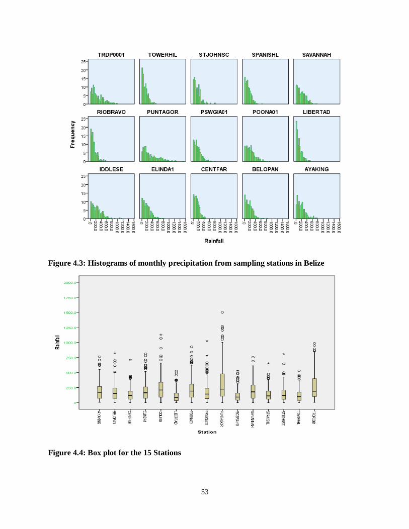
53
Figure 4.3: Histograms of monthly precipitation from sampling stations in Belize
Figure 4.4: Box plot for the 15 Stations

54
Table 4.2: Descriptive statistics for annual rainfall in Belize 1960-2011
Year Mean Median
Std.
Error of
Mean
Std.
Deviatio
n
KurtosisSkewnes
s
1960 5.07 5.04 0.99 3.43 1.54 0.99
1961 6.62 5.28 1.57 5.45 3.42 1.73
1962 5.93 4.02 1.44 4.98 0.3 0.95
1963 3.67 2.24 0.94 3.26 -0.49 0.92
1964 5.41 5.17 1.33 4.61 -2.04 0.11
1965 4.92 4.3 0.88 3.05 -0.06 0.47
1966 7.32 5.54 0.6 5.05 1.03 1.28
1967 5.53 4.82 0.56 4.54 8.66 2.35
1968 6.04 5.48 0.52 4.35 2.59 1.22
1969 7.06 5.08 0.68 6.24 2.29 1.47
1970 6.41 5.61 0.59 5.35 1.6 1.27
1971 6.43 4.72 0.72 6.49 7.13 2.39
1972 6.86 5.65 0.65 5.74 2.63 1.5
1973 6.33 5.38 0.56 5.3 0.75 1.04
1974 6.18 5.34 0.47 4.72 0.36 1.02
1975 5.02 3.08 0.59 5.68 1.37 1.49
1976 6.38 5.22 0.6 6.19 3.81 1.78
1977 6.51 4.94 0.48 4.85 1.74 1.35
1978 7.05 5.93 0.51 5.33 4.07 1.68
1979 7.84 7.72 0.54 5.61 0.75 0.86
1980 7.75 6.16 0.75 7.31 5.02 1.91
1981 7.01 4.82 0.72 7.22 3.29 1.72
1982 7.55 5.88 0.66 6.81 9.34 2.57
1983 6.28 3.94 0.61 6.31 3.6 1.85
1984 7.76 6.64 0.62 6.36 0.79 1.07
1985 6.04 4.62 0.49 5.18 7.4 2.27
1986 6.06 4.92 0.54 4.95 1.36 1.21
1987 4.91 3.32 0.58 5.03 5.14 2.11
1988 6.93 5.54 0.6 5.49 0.91 1.12
1989 6.18 5.08 0.56 5.41 1.85 1.4
1990 7.95 6.04 0.73 6.32 4.99 1.93
1991 5.19 4.95 0.41 3.76 -0.43 0.52
1992 6.34 5.85 0.37 4.41 0.76 0.97
1993 6.53 4.22 0.47 5.91 4.85 2.04
1994 5.69 4.42 0.38 4.75 1.95 1.39
1995 6.02 4.61 0.41 5.41 7.47 1.95
1996 5.3 4.27 0.31 4.11 3.88 1.57
1997 6.15 4.44 0.42 5.6 2.14 1.43
1998 6.06 4.72 0.43 5.74 5.79 2.03
1999 5.51 4.2 0.37 4.93 4.19 1.8
2000 6.12 4.49 0.44 5.87 2.88 1.53
2001 5.74 4.18 0.37 4.99 3.29 1.59
2002 5.53 4.33 0.38 4.82 5.82 2.07
2003 4.75 3.81 0.36 4.48 4.97 1.84
2004 5.1 4.32 0.28 3.54 1.61 1.07
2005 5.91 4.49 0.45 6.03 9.22 2.55
2006 7.55 6.33 0.47 6.05 3.02 1.4
2007 5.35 4.39 0.37 4.53 1.52 1.28
2008 5.99 3.95 0.44 5.53 2.66 1.49
2009 5.29 4.36 0.35 4.39 9.35 2.31
2010 5.69 4.51 0.41 5.05 1.52 1.21
2011 4.69 2.8 0.64 6.17 27.05 4.26

55
Figure 4.5: Box Plot of monthly average rainfall in Belize 1960-2011
Fitting the Wakeby Probability Distribution
The Wakeby distribution (WAD), defined by Thomas and introduced by Houghton (1977),
is defined by the quantile function
𝑥(𝐹) = 𝜉 +𝛼
𝛽[1 − (1 − 𝐹)𝛽 ] −
𝛾
𝛿[1 − (1 − 𝐹)−𝛿) ],
(4-1)
where 𝐹 = 𝐹(𝑥) = 𝑃(𝑋 ≤ 𝑥) is the cumulative distribution function. The parameterization
explicitly exhibits the WAD as a generalization of Pareto distribution when α = 0, or γ = 0), and
gives estimates of the α and γ parameters that are more stable under small perturbations of the
data. The domains of the parameters are:
ξ ≤ x ≤ ∞ if δ ≥ 0 and γ > 0 ;

56
𝜉 ≤ 𝑥 ≤ 𝜉 +𝛼
𝛽+ 𝛾/𝛿 if δ<0,or γ=0.
This distribution is defined by five parameters, more than most of the common systems
of distributions. This allows for a wider variety of shapes, and so a reasonably good fit to a
sample might be expected. Actually, by suitable choice of parameter values of WAD, it is
possible to mimic the extreme value, log-normal, generalized Pareto and log-gamma
distributions. Empirical evidence, in relation to the condition of separation (Matalas et al.,
1975), suggests that the distributions of floods are more nearly Wakeby-like with β>1 and γ>0
(i.e., long stretched upper tails) than like any of the other more commonly suggested flood
distributions (Houghton, 1978; Landwehr et al., 1978). In addition, WAD provides a plausible
description of precipitation sequences, and it also provides a means for representing the
seemingly long, stretched upper tail structures of flood distributions, as well as the tail structures
of distributions of other hydrologic phenomena (Landwehr et al., 1980). Thus WAD can credibly
be considered a parent hydrology distribution. Because of the above reasons, WAD is widely and
successfully used in hydrology, especially for the modelling of extreme events. Recently, Wilks
and McKay (1996) concluded that WAD provided the best representations of extreme snowpack
water equivalent values, based on the performance evaluation of a suite of theoretical probability
distributions.
For estimation of the five parameters of WAD, the method of L-moments estimation (Hosking,
1990) has been used. In this study, attempts to use WAD with the method of L-moments
estimates(L-ME), on the Belize’s rainfall data (monthly average precipitation) at 15 weather
stations Belize have been made to obtain reliable quantile estimates.

57
Figure 4.6: Histogram of Monthly Rainfall from sampling stations in Belize (1964-2011)
The Wakeby Probability distribution is a very flexible five-parameter distribution (Pilon
and Harvey,
1994). It can assume shapes that other distributions cannot describe. While this has been seen as
an advantage, it means that records with several years of extreme data can affect the shape of this
distribution to a greater extent than other distributions

58
L- Moment Estimation of Wakeby Probability Distribution
For estimation of the five parameters of WAD, the method of L-moments estimation
(Hosking, 1990) has been used. Since the distribution function F(x) of WAD is not explicitly
defined, the maximum likelihood estimates (MLE) of parameters are not easily obtained (see
Park and Jeon, 2000, for computing MLE).Thus the method of probability weighted moments
(PWM) estimation was introduced by Greenwood et al. (1979) for estimation of parameters of
the distributions (like WAD) whose inverse form x = x(F) is explicitly defined. Since the L-
moments are simple linear combinations of special cases of PWMs, the method of L-moments
estimation (L-ME) can be viewed as equivalent to the method of PWM estimation. L-Moments
are more convenient, however, because they are more directly interpretable as measures of the
scale and shape of the probability distribution. The main advantages of using L-ME are that the
parameter estimates are more reliable than the method of moment’s estimates, particularly from
small samples, and are usually computationally more tractable than MLE. Furthermore, due to
the use of linear moments instead of the conventional product moments and being resistant to the
presence of outliers (which may be present in the sample due to the occurrence of heavy rainfall
and typhoon events), the method is quite robust.
The (population) L-moments of WAD are, following Hosking (1986):
𝜆1 = 𝜉 +𝛼
1 + 𝛽+
𝛾
𝛿 − 1
(4-2)
𝜆2 =𝛼
(1 + 𝛽)(2 + 𝛽))+
𝛾
(1 − 𝛿)(2 − 𝛿)
(4-3)

59
𝜆3 =
𝛼(1 − 𝛽)
(1 + 𝛽)(2 + 𝛽)(3 + 𝛽))+
𝛾(1 + 𝛿)
(1 − 𝛿)(2 − 𝛿)(3 − 𝛿)
(4-4)
𝜆4 =
𝛼(1 − 𝛽)(2 − 𝛽)
(1 + 𝛽)(2 + 𝛽)(3 + 𝛽)(4 + 𝛽))+
𝛾(1 + 𝛿)(2 + 𝛿)
(1 − 𝛿)(2 − 𝛿)(3 − 𝛿)(4 − 𝛿)
(4-5)
𝜆𝑟 =
𝛼Γ(1 + 𝛽)Γ(𝑟 − 1 − 𝛽)
Γ(1 − 𝛽)Γ(𝑟 + 1 + 𝛽)+𝛾Γ((1 − 𝛿)Γ((𝑟 − 1 + 𝛿)
Γ(1 + 𝛿)Γ(𝑟 + 1 − 𝛿), 𝑟 ≥ 5
(4-6)
The sample L-moments are obtained from observations: see Hosking (1990) for the
formulas. Now, analogously to the usual method of moment’s estimations, the ‘method of L-
moments estimation’ (L-ME) obtains parameter estimates by equating the first p (number of
parameters) sample L-moments to the corresponding population L-moments. Since no explicit
solution of simultaneous equations is possible in WAD, the equations can be solved by Newton–
Raphson iteration. Landwehr et al. (1979) derived an algorithm to get the estimates in each of the
cases: known and unknown. The FORTRAN program (PELWAK) provided by Hosking (1997)
basically uses the method of Landwehr et al. (1979). First a solution is sought in which all five
parameters are estimated, as functions of the first five L-moments. If no solution is found due to
convergence failure, the parameter it is set to zero and a solution is sought in which the other
four parameters are estimated as functions of the first four L-moments. If this too is
unsuccessful, then a generalized Pareto distribution is fitted instead, using the first three L-
moments. Note that, when α=0 or γ=0 (but not simultaneously) in WAD, Equation (4.1) is
reduced to the following quantile function of the generalized Pareto distribution:
𝑥(𝐹) = 𝜉 + 𝛼[1 − (1 − 𝐹)𝑘]/𝑘
(4-7)

60
The probability function, the parameter estimates (L-ME) of WAD, and Kolmogorov–
Smirnov’s (K–S) goodness-of-fit statistic D at each station are given in Tables 4.3. The p-values
of K–S Ds are at least 0.35, which shows that WAD is acceptable for each of the stations. Figure
3-3 shows the relative frequency histogram of each station.
Result of Fitting The Wakeby Probability Distribution Function
Table 4.3: Station codes, parameters estimates of Wakeby Distribution, K_S statistics and
P-Value computed from Stations.
Table 4.4: Best fit probability distribution of clustered data
ξ α β γ δ K/S P-VALUE
BELOPAN GENERALIZED PARETO/WAKEBY 0.06683 7.8054 0.37647 0 1.2X10⁻¹⁰ 0.04798 0.28331MAYAKING WAKEBY 0.2323 8.6237 0.47852 0.05272 0.84023 0.0317 0.98577CENTFAR WAKEBY 0.14455 6.8201 1.5701 1.6727 0.13124 0.01716 0.99674MELINDA1 WAKEBY 0.03842 7.8997 0.87932 1.5684 0.20613 0.02196 0.9789MIDDLESE WAKEBY 0.06274 10.976 0.67555 0.94254 0.34904 0.01871 0.99717LIBERTAD GENERALIZED PARETO/WAKEBY 0.01904 1.4785 8.919 4.4148 0.1539 0.03011 0.97781POMONA01
WAKEBY 0.08723 8.0197 2.0053 4.8682 0.05419 0.0176 0.99736PSWGIA01 WAKEBY 0.05753 7.0258 0.92207 1.8704 0.20133 0.00953 0.91149PUNTAGOR WAKEBY 0.06185 5.8544 1.5634 3.7473 0.11954 0.00894 0.91251RIOBRAVO WAKEBY 0.06585 5.5682 1.5095 3.7005 0.11986 0.00855 0.9238SAVANNAH WAKEBY 0.05679 5.7091 1.2799 3.4331 0.1255 0.00867 0.8856SPANISHL WAKEBY 0.06124 5.5102 1.4464 3.5116 0.11687 0.00901 0.80836STJOHNSC WAKEBY 0.0614 5.4668 1.4131 3.4384 0.12145 0.00894 0.80014TOWERHIL WAKEBY 0.0718 5.4613 1.2762 3.153 0.14236 0.00833 0.84247TRDP0001 WAKEBY 0.070336 4.971 1.6027 3.8992 0.01957 0.00793 0.8267
PARAMETERS
Stations BEST- FIT Distribution
Goodness of fit
ξ α β γ δ K/S P-VALUEBELOPAN 1SPANISHL 1LIBERTAD 2TOWERHIL 2MELINDA1 3POMONA01 3PSWGIA01 4STJOHNSC 4SAVANNAH 6 WAKEBY 0.05679 5.7091 1.2799 3.4331 0.1255 0.00867 0.8856TRDP0001 7 WAKEBY 0.070336 4.971 1.6027 3.8992 0.01957 0.00793 0.8267PUNTAGOR 8 WAKEBY 0.06185 5.8544 1.5634 3.7473 0.11954 0.00894 0.91251
WAKEBY
WAKEBY
WAKEBY
PARAMETERS
WAKEBY-0.05716 4.9758 1.3827 3.619 0.11986 0.00869 0.86718
0 -4.5897 3.189 4.7423 -0.21757 0.03027 0.731
0.01631 0.98273
0.0536 7.6303 1.5533 3.3554 0.04328 0.01679 0.9493
-0.01513 6.8051 0.90516 1.2907 0.26009
BEST- FIT
DistributionClustersStations
Goodness of fit

61
Hydrological data are often asymmetrical and right skewed. Results from fitting data,
from the meteorological stations and the results represented in short by the following paragraphs.
The method discussed above is used to estimate the parameters of the Wakeby Distribution for
the period 1960 -2012. In addition to the Wakeby Distribution, efforts were made to test the
performance of other popular distributions such as lognormal and Weibull distribution. The
estimated parameters for the Wakeby Distribution are presented in Table 4.3. From the Table
4.3, it appears that the data fits the identified Wakeby distribution well. Table 4.5 compares the
actual observed average rainfall for each station to that of the estimated average rainfall using
our proposed model. It is showed that the range of the difference is from (0 - 48.59) %, with an
average difference of 20.52%. In Table 4.6, we compared the actual average monthly rainfall to
Table 4.5: Comparison of station’s observed average vs. proposed model estimated average
rainfall
Stations Mean Wakeby Mean % Difference
BELMOPAN 5.74 5.74 0.01
CENTFAR 4.45 4.72 6.03
LIBERTAD 3.70 5.39 37.22
MAYAKING 6.39 6.39 0.00
MELINDA1 6.14 6.22 1.24
MIDDELSE 7.94 8.06 1.57
POMONA01 7.20 7.90 9.32
PSWGIA01 5.43 6.05 10.83
PUNTAGOR 10.51 6.60 45.67
RIOBRAVO 3.95 6.49 48.59
SAVANNAH 6.54 6.49 0.89
SPANISHL 4.31 6.29 37.43
STJOHNSC 4.81 6.24 25.87
TOWERHIL 3.81 6.15 47.01
TRDP0001 8.59 5.96 36.19

62
Table 4.6: Comparison of station’s observed average vs. PRECIS model forecasted average
rainfall
the PRECIS forecasted values for the stations. This this second comparison the range of the
difference is (33.64- 40.98) %, with an average difference of 38.58 in the average monthly
rainfall for the stations. The selection of an appropriate frequency distribution for extreme
precipitation over Belize is made with an aim to identify a distribution that best fits the observed
data.
Examining Belize’s Wet and Dry Seasons
Since there are two distinct rainfall seasons in Belize, we test whether there is a significant
difference between the Wet and Dry season in Belize. The Kruskal Wallis test and the
Kolmogorov Smirnov test suggested that there is a statistical significant difference between the
two seasons hence the need to further examine the p. d. f. of the two seasons. Table 4.8 shows
that for the dry season the best fit model is the Wakeby distribution; however, for the Wet season
Stations Mean PRECIS
% Difference
BELMOPAN 5.74 8.06 33.64
CENTFAR 4.45 6.63 39.44
LIBERTAD 3.70 5.73 43.09
MAYAKING 6.39 9.26 36.62
MELINDA1 6.14 9.05 38.32
MIDDELSE 7.94 11.12 33.43
POMONA01 7.20 10.80 40.04
PSWGIA01 5.43 8.16 40.18
PUNTAGOR 10.51 15.92 40.98
RIOBRAVO 3.95 5.59 34.36
SAVANNAH 6.54 10.05 42.21
SPANISHL 4.31 **** ****
STJOHNSC 4.81 7.19 39.63
TOWERHIL 3.81 5.70 39.86
TRDP0001 8.59 12.66 38.30

63
from June to November the average rainfall in Belize from 1964-2011 follows a Generalized
extreme value distribution. Figure 4.7 and 4.8 shows the p.d.f. of the two seasons.
Table 4.7: Hypothesis Test Summary
Table 4.8: Best Fit Model for the monthly rainfall
Dry Wakeby 0.0112 0.86425
Wet Gen. Extreme Value 0.01264 0.75285
Best fit probability distribution for Belize's
average monthly rainfall by season
Season
Best fit
Distribut
ion
Kolmogorov
Smirnov StatisticsP-value
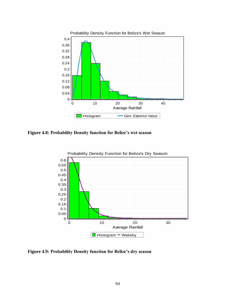
64
Figure 4.8: Probability Density function for Belize’s wet season
Figure 4.9: Probability Density function for Belize’s dry season
Probability Density Function for Belize's Wet Season
Histogram Gen. Extreme Value
Average Rainfall
403020100
f(x)
0.4
0.36
0.32
0.28
0.24
0.2
0.16
0.12
0.08
0.04
0
Probability Density Function for Belize's Dry Season
Histogram Wakeby
Average Rainfall
3020100
f(x)
0.6
0.55
0.5
0.45
0.4
0.35
0.3
0.25
0.2
0.15
0.1
0.05
0

65
Conclusion
The determination of the best fit distribution to represent the rainfall process in stations of
Belize is discussed in this paper. The an extensive search comparing several distribution such
as Wakeby , lognormal, gamma, Weibull ,Generalized Pareto, Dugan and many other
distributions have been used on the monthly average rainfall data from 1960 to 2011. The
selection of the best fit distribution is done by examining the minimum error produced by the
Kolmogorov Smirnov (KS) goodness of fit test. Based on the results of KS goodness of fit test,
Wakeby distribution is the most suitable to describe the rainfall patterns in the stations of Belize
as the error produced is the minimum. There were three stations, Belmopan, Libertad and Rio
Bravo for which the Wakeby distribution was ranked as second best distribution.
The cluster analysis identifies eight clusters in Belize’s rainfall using the Ward’s Method
(See Table 4.4). Four of the clusters are somewhat notable because their clustering is based on
their regional location such north, south, central and west. Looking at the individual best fit
probability distribution functions of the clusters, notably the Wakeby distribution base on the
Kolmogorov Smirnov test statistics fitted the data very well. Therefore, the best fit probability
function is the Wakeby distribution. The variation exhibit permits for the further study of the
underlying factors present in the different geographical area in Belize.

66
Chapter 5: Statistical Models for Forecasting Tourists Arrival in Belize
Introduction
In the previous chapter we understand the behavior of rainfall of Belize and this is very
important to tourism. Tourism is vitally important to the entire Belizean economy, contributing
26% of Belize's gross domestic product in 2006 and 50% in 2015. In most of coastal Belize,
tourism has completely replaced fishing as the primary source of income for all but a very few
residents. Tourism is the number one foreign exchange earner in this small economy, followed
by exports of marine products, citrus, cane sugar, bananas, and garments. However, this sector is
exposed to the vagaries of international economics and is severely affected in recession years.
Despite the drop in arrivals in 2009 the industry experienced many record breaking arrivals
which led to an overall growth during the years 2011- 2015, an outstanding period for the Tourism
Industry in Belize.
The development of tourism in Belize was premised originally on the niche marketing of
the country to high end, stay-over visitors interested in a pristine, natural, land and marine
environment, otherwise known as eco-tourism. The consequent pressures on tourism facilities,
sites and regulatory capacity generated by these day visitors sparked controversial debates on the
potential negative impact on the niche stay-over market segment, highlighted the problems
arising from the lack of a cohesive, comprehensive, national framework for tourism/cruise
development and raised questions on the actual net benefits accruing to Belize from mass
market, cruise tourism. The development of the tourism industry in Belize was built through the
development of the overnight sector. Over the past five years. Belize overnight tourism sector

67
has seen consistent growth, and particularly very strong performances in 2012-2014, with 2014
being the most positive year of overnight tourism in Belize in the last ten years.
The forecast of tourists’ arrival is important since it would enable the tourism industry of
Belize to adequately prepare for any number of arrivals at any future date. The benefits of
accurate forecast s are well documented in tourism forecasting literature (Molly 1991). Accurate
forecasts are valuable to both the private and public sectors. Forecasting is crucial for the private
sector in planning to avoid shortages or surpluses in goods and services. Time series analysis and
modelling plays a very important role in forecasting, especially when our initial stochastic
realization is nonstationary in nature.
Time series analysis is one of the major areas in statistics that can be applied to many
realistic problems. In the present chapter, we begin with a description of the structure of the
Belizean economy and the importance of tourism in the economy. We then summarize the
development of time series modeling and introduce some methodologies that have been
developed recently. We also introduce some fundamental concepts that are essential for dealing
with time series models. We carry out a statistical comparison of two different time series
models by comparing their forecasting and actual residuals.
A true test of a forecasting model is its ability to forecast outside the sample period. We
measure the accuracy of the forecasts by withholding the data for the last two years. We use for
each model a subset of the data (all observations except the last two years) to forecast the
remainder of the known data. For the forecast period, a forecast error is calculated, defined as
actual tourist arrivals less forecast tourist arrivals. We then used the mean absolute percentage
error (MAPE), as the final measure of forecast accuracy.

68
Over the past two decades, the study of air travel demand forecasting has attracted
considerable attention by researchers. Within the Central American and Caribbean region
considerable attention has been given to tourism but not much in terms of statistical driven
research. For Belize, the last known study was done by United Nation in 1992 where they
forecasted Caribbean tourist data using ARIMA. Among various competing forecasting models,
ARIMA has gained popularity and is frequently adopted in empirical studies, because it often
outperforms many other econometric and time series methods. Dharmaratne (1995) estimates
and validates the ARIMA model for forecasting long-stay visitors in Barbados and suggests that
customized model building may be highly rewarding compared to simple or standard methods.
Lim and McAleer (1999) use the ARIMA model to explain tourist arrivals from Malaysia to
Australia. The HEGY seasonal unit roots test is used to examine stochastic seasonality in the
tourism demand series. Their findings, revealing the existence of seasonal unit roots in
international tourist arrivals from Malaysia to Australia, is evidence in favor of a varying, rather
than constant seasonal pattern. Kulendran and Witt (2003) examine seven forecasting models on
international business tourism and suggest that the relative forecasting performance of various
models is highly dependent on the length of forecasting horizon and the detection of seasonal
unit roots. In addition, the Lim and Pan (2005) study also adopts the ARIMA model to study
inbound tourism development in China. A comparison of the forecasting performance of
competing models is frequently highlighted in recent tourism demand forecasting literature (Chu
2004, Kulendran and Wong 2005, Coshall 2006). While consensus is not yet achieved, many
researchers conclude the ARIMA model, to a great degree, appears the suitable model (Chu
1998, Kim and Song 1998, Kulendran and Witt 2001, Lim and McAleer 2002). For the purpose

69
of forecasting performance comparison, we choose two models including Seasonal ARIMA and
the Holt–Winter method to model inbound tourism arrival in Belize.
Structure of Belize’s Economy and Importance of Tourism
With a GDP of $9600 per capita in 2014, Belize is a small, open economy, characterized
by a narrow production base, heavy reliance on imports, small range of mostly primary, export
commodities and a manufacturing capacity (excluding export sugar and citrus juice
manufacturing) limited to production which can profitably meet the domestic demand of its
small population base (0.37million people in 2015).
Up to the 1990’s, the country was highly dependent on sugar exports that accounted for more
than 40.0% on average of domestic merchandise exports. Following the oil shock in the late
1970’s and plummeting sugar prices in the early 1980’s, the development of the tourism industry
was encouraged as part of a general strategy to diversify the economy, increase foreign exchange
earnings, generate employment and so improve the country’s resilience to external shocks.
After more than four decades, some success in reducing dependence on sugar exports and
in expanding the tourism industry was achieved. Sugar as a share of domestic exports went from
44.7% in 1984 to 25.1% in 2015 with a low of 10.9% in 2010, in response to higher production
of other traditional exports such as citrus and banana and development of nontraditional
commodities such as papaya, farmed shrimp and petroleum. Meanwhile, significant foreign and
local investments into tourism have gradually raised its economic importance and have
contributed to its current substantial level.
The results of the continued tourism expansions are evident. Foreign exchange earnings
as a percent of exports of goods and services have increased. Using the SIC categories of “Hotel

70
and Restaurants” and “Transportation” to proxy tourism’s contribution to GDP, Its share of GDP
increased over the same period. Employment in tourism has risen steadily with time. Available
data since 1998 showed that employment in tourism rose from one out of every 11 persons in
1998 to one out of every 7 persons by 2014 (BTB 2014).
Table 5.1: Belize’s Economics as it relates to Tourism
Belize’s Economics as it relates to Tourism
%
change
'14 vs.
'13 2014 2013 2012 2011 2010
Tourist Expenditure (mnBze $) 3.2 773 750 639 514 500
Tourist Expenditure (mn US $) 3.2 387 375 320 257 250
Employment in Tourism (SIB) 19,141 18,850 N.D. N.D. 13,242
Total Employment (SIB) 4.8 134,421 128,277 N.D. N.D. 107,484
Tourism employment as a % of total -3.1 14.2 14.7 N.D. N.D. 12.3
GDP - Current Prices (mnBze $) - revised 4.6 3,398 3,249 3,145 2,978 2,797
Tourism expenditure as % of GDP 22.8 23.1 20.3 17.2 17.9
Total 1699 1624.3 1572.6
Institutional and Policy Framework
The Belize Tourism Board (BTB) is the implementing arm of the Ministry of Tourism.
Responsibility for planning, developing, promoting and regulating the growth of the tourist
industry lies with this statutory body whose Board of Directors is comprised of private sector
representatives and whose budget is funded through industry taxes.
In addition to the work of the BTB, Government provides assistance mostly through loan funded
projects that address critical infrastructural constraints. Between 2000 and 2004, the
Government, through a combination of loan, grants and counterpart funds, invested

71
approximatelyUS$15.0 million to develop and improve a number of major archaeological sites
and provide training mostly to tour guides and other service providers. Notably, the
improvements to the archaeological sites were designed for a combined maximum of 300,000
cruise and stay-over visitors and did not cater for the explosive growth in cruise arrivals that
began in 2002.Various private sector associations, funded through membership fees, protect and
lobby for their interests. The Belize Tourism Industry Association (BTIA) was initially set up as
an umbrella organization for all service providers. Its membership includes various smaller
associations such as the Hotel and Tour Guides Association. The Federation of Cruise
Associations of Belize is a recently formed breakaway group consisting of some 800 members
spread across 19 associations that include tendering, taxis, handicraft and transportation. The
members of this federation did not want their interests diluted by biases in favor of stay-over
market interests.
Recognizing the need for a comprehensive framework and more pro-active approach to
developing the tourism industry, the Ministry of Tourism commissioned the Blackstone
Corporation in 1998 to develop a ten year strategy and action plan to stimulate economic growth,
while protecting the country’s environmental and heritage resources and ensuring benefits for the
local people.
This first national tourism strategy recommended the continued niche marketing of the
country to high-end spenders on an eco-tourism platform that promoted small scale,
environmental, cultural and community tourism with strong inter-sectoral linkages. The
Blackstone report considered and discarded a mass tourism scenario aimed at quadrupling
arrivals to 400,000 by2008, because it was felt that the environmental degradation and negative
cultural impact could destroy the country’s eco-tourism niche. Instead, the proposed strategy

72
opted for a lower, average, annual growth of 4.0% or minimum target of 120,000 visitors by the
end of the first 5years and a minimum of 140,000 visitors by the end of 2008.
An updated national tourism policy (BTB, 2005) was crafted in 2005 that recommended
the non-conflicting co-existence of the niche, stay-over and mass market, cruise segments. The
policy assumed that cruise arrivals would stabilize at an annual rate of 1.0mn visitors and
cautioned that the expansion of the cruise industry should not jeopardize Belize’s status as an
eco-tourism destination. It suggested that selected sites should be designated primarily as cruise
visitors’ sites or new sites catering specifically to the cruise market should be developed.
Another recommendation was the immediate implementation of ceilings or capacity limits on the
number of cruise visitors to designated sites. This policy also called for the development of a
long term Tourism Master Plan (a plan of action, cutting across all government ministries and
even some private sector stakeholders) to implement the recommendations suggested in the
policy paper. To date, no sites have been designated specifically for cruise tourists, nor have
capacity limits been adhered to and financing constraints have delayed development of the
master plan.
The Government, however, has secured a loan to finance tourism oriented infrastructural
projects in selected destinations and has also produced the tourism master plan. It remains to be
seen if the needed multi-disciplinary buy-in will be obtained to implement the entire policy
rather than just those sections that fall within the purview of the tourism ministry and the BTB,
as happened with the 1998 strategy. Notwithstanding the existence of this policy, the sentiment is
widely felt especially among the stakeholders in the stay-over market that the explosive growth
of cruise tourism has put at risk the country’s niche positioning as a high-end provider of an eco-

73
based tourist experience, and its development has not proceeded in a sustainable and
environmentally responsible manner.
Significant attention was given to the cruise tourism because of the potential and contributions to
the countries’ economy and in 2015 there was a total of 957,975 Cruise Passenger Arrival, this
was a minor drop pf 1% compared to 2015.
Figure 5.1 shows that Americans continue to be our largest market for visitors, making up 63.1%
of the overall arrivals. This followed by Europeans at 12% and Canadians at 7% in 2015.
Figure 5.1: Market Share: Jan – Dec 2015
Methodology
Figure 5.2 shows the actual data used in the model building process and illustrates the high
degree of nonlinearity and seasonality and upward trend in time. The time plot shows drop in
Americans 63.1%
All Europeans 12.0%
Canadians 7.0%
Belizeans living abroad
4.4% Guatemalans
2.7% Mexicans
2.0%
Central America* 2.9%
Caribbean 0.8%
South America 1.4%
Asia 1.2%
Middle East 0.7% Africa
0.2%
Oceania 1.6%
Other 8.8%
Market Share: Jan-Dec 2015
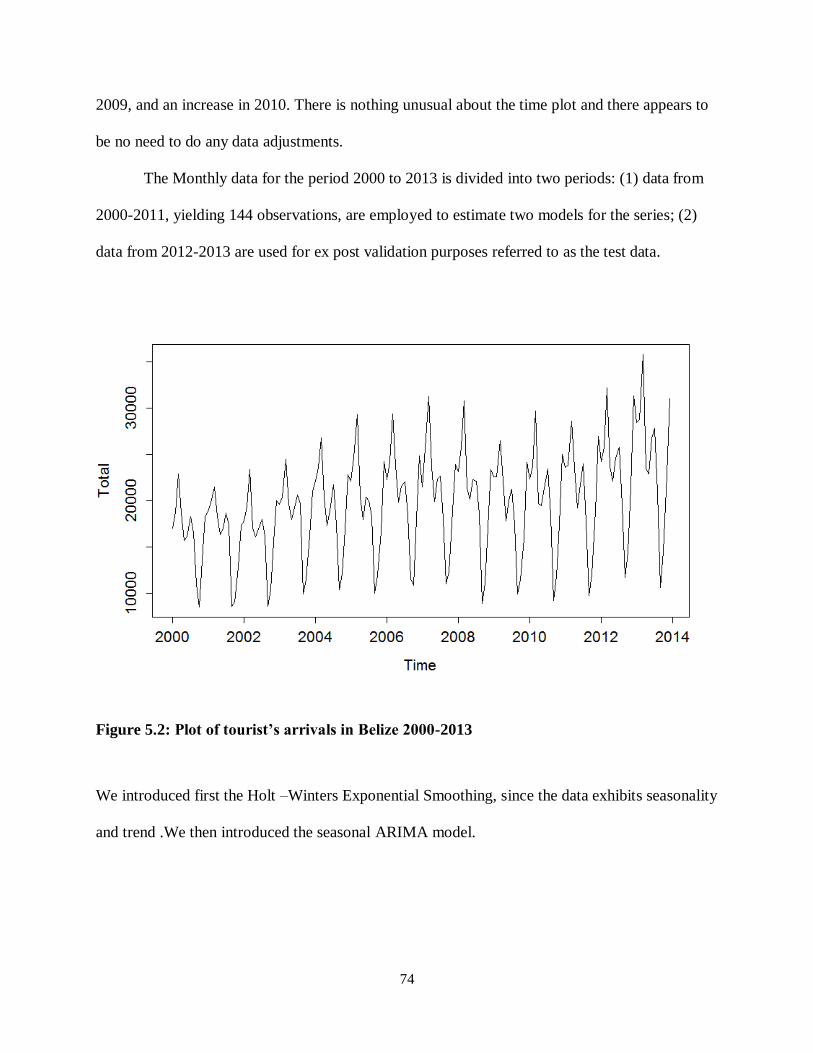
74
2009, and an increase in 2010. There is nothing unusual about the time plot and there appears to
be no need to do any data adjustments.
The Monthly data for the period 2000 to 2013 is divided into two periods: (1) data from
2000-2011, yielding 144 observations, are employed to estimate two models for the series; (2)
data from 2012-2013 are used for ex post validation purposes referred to as the test data.
Figure 5.2: Plot of tourist’s arrivals in Belize 2000-2013
We introduced first the Holt –Winters Exponential Smoothing, since the data exhibits seasonality
and trend .We then introduced the seasonal ARIMA model.
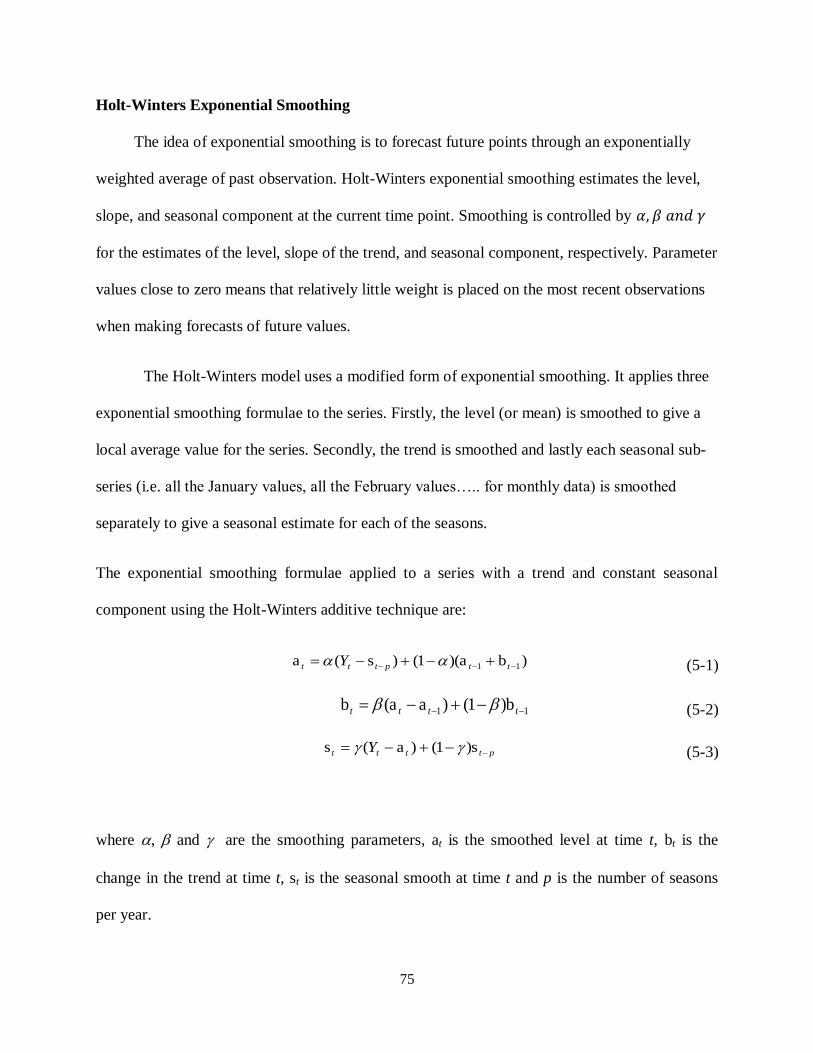
75
Holt-Winters Exponential Smoothing
The idea of exponential smoothing is to forecast future points through an exponentially
weighted average of past observation. Holt-Winters exponential smoothing estimates the level,
slope, and seasonal component at the current time point. Smoothing is controlled by 𝛼, 𝛽 𝑎𝑛𝑑 𝛾
for the estimates of the level, slope of the trend, and seasonal component, respectively. Parameter
values close to zero means that relatively little weight is placed on the most recent observations
when making forecasts of future values.
The Holt-Winters model uses a modified form of exponential smoothing. It applies three
exponential smoothing formulae to the series. Firstly, the level (or mean) is smoothed to give a
local average value for the series. Secondly, the trend is smoothed and lastly each seasonal sub-
series (i.e. all the January values, all the February values….. for monthly data) is smoothed
separately to give a seasonal estimate for each of the seasons.
The exponential smoothing formulae applied to a series with a trend and constant seasonal
component using the Holt-Winters additive technique are:
)b)(a1()s(a 11 ttpttt Y (5-1)
11 )b1()a(ab tttt (5-2)
ptttt Y )s1()a(s
(5-3)
where , and are the smoothing parameters, at is the smoothed level at time t, bt is the
change in the trend at time t, st is the seasonal smooth at time t and p is the number of seasons
per year.

76
The Holt-Winters algorithm requires starting (or initialising) values. Most commonly:
)(
1a 21 pp YYY
p
(5-4)
p
YY
p
YY
p
YY
p
ppppp
p 22111
b �
(5-5)
ppppp YsYsY a , ,a ,as 2211 � (5-6)
the Holt-Winters forecasts are then calculated using the latest estimates from the appropriate
exponential smoothings that have been applied to the series. So we have our forecast for time
period T :
TTTTy sbaˆ (5-7)
where Ta is the smoothed estimate of the level at time T, Tb is the smoothed estimate of the
change in the trend value at time T and Ts is the smoothed estimate of the appropriate seasonal
component at T.
As mentioned earlier the Holt-Winters model assumes that the seasonal pattern is relatively
constant over the time period. We expected to notice changes in the seasonal pattern and
identify this as a potential problem with the model, particularly if long–term predictions are
made. In practice this is dealt with by transforming the original data and modelling the
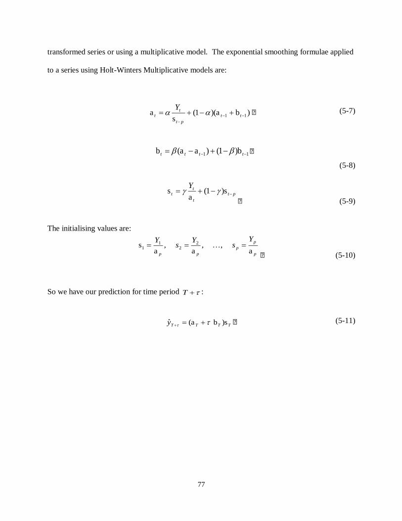
77
transformed series or using a multiplicative model. The exponential smoothing formulae applied
to a series using Holt-Winters Multiplicative models are:
)b)(a1(s
a 11
tt
pt
t
t
Y �
(5-7)
11 )b1()a(ab tttt �
(5-8)
pt
t
tt
Y )s1(
as
� (5-9)
The initialising values are:
p
p
p
pp
Ys
Ys
Y
a , ,
a ,
as 2
21
1
� (5-10)
So we have our prediction for time period T :
TTTTy )sb(aˆ �
(5-11)

78
Figure 5.3: Plot of Tourist arrivals two year forecast
ARIMA Model
The classical ARIMA (p, d, q) is defined as follows
∅𝑝(𝐵)(1 − 𝐵)𝑑𝑋𝑡 = 𝜃𝑞(𝐵)휀𝑡 (5-12)
Where {𝑋𝑡} is the realized time series.
The seasonal ARIMA model incorporates both non-seasonal and seasonal factors in a
multiplicative model. One shorthand notation for the model is ARIMA (p, d, q) × (P, D, Q)S,
with p = non-seasonal AR order, d = non-seasonal differencing, q = non-seasonal MA order, P =
seasonal AR order, D = seasonal differencing, Q = seasonal MA order, and S = time span of
repeating seasonal pattern. Without differencing operations, the model could be written more
formally as
𝛷(𝐵𝑆)𝜑(𝐵)(𝑋𝑡 − 휀𝑡) = 𝛩(𝐵𝑆)𝜃(𝐵)휀𝑡 (5-13)
Plot of tourist's arrival two year forecast
TIME
Tour
ist A
rriva
ls
2000 2002 2004 2006 2008 2010 2012 2014
1000
015
000
2000
025
000
3000
0

79
The non-seasonal components are:
AR: φ(B) = 1 - φ1B - ... - φpBp
MA: θ(B) = 1 + θ1B + ... + θqBq
The seasonal components are:
Seasonal AR: Φ(BS) = 1 - Φ1B
S - ... - ΦPBP
S
Seasonal MA: Θ(BS) = 1 + Θ1B
S + ... + ΘQBQ
S
Note that on the left side of Equation (5.1) the seasonal and non-seasonal AR components
multiply each other, and on the right side of Equation (5.1) the seasonal and non-seasonal MA
components multiply each.
The order of the seasonal ARIMA model determines the structure of the model and it is
essential to have a good methodology in terms of developing the forecasting model. In the
present study, we start with addressing the issue of the seasonal sub index s. After we examine
the original data, shown by Figure 5.11, we have reason to believe the average monthly tourists
arrivals behave as a periodic function with a cycle of 12 months.
Hence, we let the seasonal sub index s = 12. In time series analysis, one cannot proceed
with a model building procedure without confirming the stationarity of a given stochastic
realization, thus, we test the overall stationarity of the series by using the method introduced by
Kwiatkowski, D., Phillips, P C. B., Schmidt, P., and Shin, Y in 1992, (Kwiatkowski et al., 1992).
Once the order of the differencing is identified, it is common for one ARIMA ( p, d, q)
×(P,D,Q)s model that we have several sets of ( p, q, P, Q)that are all adequately representing a
given set of time series. Akaike’s information criterion, AIC, (Akaike, 1974), was first

80
introduced by Akaike in 1974 plays a major role in our model selecting process. We shall choose
the set of (p, q, P, Q) that produces the smallest AIC.
Another important aspect in our model selection process is to determine the seasonal
differencing, D, the goal is to select a smaller AIC without complicating the selected model.
Hence, we only compute the AIC for both D = 0 and D = 1 based on our previous selection of
the orders (p, d, q, P, Q), and choose the model with smaller AIC to be our final model.
Below we summarize the model identifying procedure:
1. Determine the seasonal period s.
2. Check for stationarity of the given time series 𝑦𝑡 by determining the order of
differencing d, where d = 0, 1, 2,…, according to KPSS test, until we achieve stationarity.
3. Deciding the order m of the process, for our case, we let where m= 5
p + q + P + Q ≤m
4. After (d, m) are selected, lies all possible configurations of ( p, q, P, Q) for
p + q + P + Q ≤m
5. For each set of ( p, q, P, Q) , estimate the parameters for each model, that is,
∅1 , ∅2 , … , ∅𝑝 , 𝜃1𝜃2, … , 𝜃𝑞 , Φ1, Φ2, …Φ𝑝
6. Compute the AIC for each model, and choose the one with smallest AIC.
7. After (p, d, q, P, Q) is selected, we determine the seasonal differencing filter by selecting
the smaller AIC between the model with D = 0 and D = 1.
8. Our final model will have identified the order of (p, d, q, P, D, Q).
With the use of statistical software such are R.

81
Figure 5.4: Plot of tourist’s arrival in between 2000 - 2013 and forecast
Comparison of the Forecasting Models
Diagnostic checks help to determine if the anticipated model is adequate. At this stage, an
examination of the residuals from the fitted model is done and if it fails the diagnostic tests, it is
rejected and we repeat the cycle until an appropriate model is achieved. Different combinations
of AR and MA individually yield different ARIMA models. The optimal model is obtained on
the basis of minimum value of Akaike Information Criteria (AIC). The Root Mean Square Error
(RMSE) and the Mean Absolute Percentage Error (MAPE) are used to evaluate the performance
of the various models and are given below. For comparing the forecasting performance of
competing models, the measure of accuracy of mean absolute percent error (MAPE) is calculated
as:
𝑀𝐴𝑃𝐸 =
1
𝑛∑|
𝑌𝑡 − 𝐹𝑡𝑌𝑡
| ∗ 100
𝑛
𝑡=1
(5-14)
Where yt (t=1, 2 . . . n) is the actual value, and F(t= 1, 2, . . , n) represents the forecasted value.
The lower the value of MAPE is, the better the forecast will be. According to Lewis
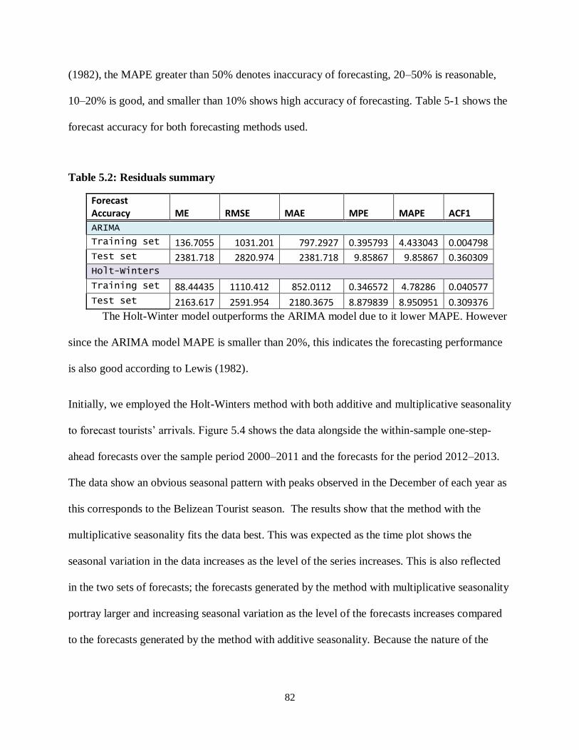
82
(1982), the MAPE greater than 50% denotes inaccuracy of forecasting, 20–50% is reasonable,
10–20% is good, and smaller than 10% shows high accuracy of forecasting. Table 5-1 shows the
forecast accuracy for both forecasting methods used.
Table 5.2: Residuals summary
Forecast Accuracy ME RMSE MAE MPE MAPE ACF1
ARIMA
Training set 136.7055 1031.201 797.2927 0.395793 4.433043 0.004798
Test set 2381.718 2820.974 2381.718 9.85867 9.85867 0.360309 Holt-Winters
Training set 88.44435 1110.412 852.0112 0.346572 4.78286 0.040577
Test set 2163.617 2591.954 2180.3675 8.879839 8.950951 0.309376
The Holt-Winter model outperforms the ARIMA model due to it lower MAPE. However
since the ARIMA model MAPE is smaller than 20%, this indicates the forecasting performance
is also good according to Lewis (1982).
Initially, we employed the Holt-Winters method with both additive and multiplicative seasonality
to forecast tourists’ arrivals. Figure 5.4 shows the data alongside the within-sample one-step-
ahead forecasts over the sample period 2000–2011 and the forecasts for the period 2012–2013.
The data show an obvious seasonal pattern with peaks observed in the December of each year as
this corresponds to the Belizean Tourist season. The results show that the method with the
multiplicative seasonality fits the data best. This was expected as the time plot shows the
seasonal variation in the data increases as the level of the series increases. This is also reflected
in the two sets of forecasts; the forecasts generated by the method with multiplicative seasonality
portray larger and increasing seasonal variation as the level of the forecasts increases compared
to the forecasts generated by the method with additive seasonality. Because the nature of the

83
data, we utilized the multiplicative method for further forecasting. Figure 5.5 shows the graph of
the estimated Holt Winter model and its two year ahead forecast.
The application of the method with multiplicative seasonality is presented in Table 5.2 and
Figure. Table 5.2 summarized the two year period ahead forecast values with 80% and 90%
confidence intervals for the predicted values and the actual tourist arrivals for the same period.
Figure 5.5: Forecast from H-W multiplicative model
Forecasts from Holt-Winters' multiplicative method
Year
Tour
ist v
isito
r Arri
val in
Bel
ize (T
hous
ands
)
2000 2002 2004 2006 2008 2010 2012 2014
1000
015
000
2000
025
000
3000
0
data
Holt Winters' Additive
Holt Winters' Multiplicative

84
Figure 5.6: Forecasts from Holt Winters model
Table 5.4 shows the actual tourists’ arrival and forecasted monthly tourists’ arrival in
Belize for period 2000-2013 using both the exponential smoothing and the ARIMA models. The
time plot in Figure 5.1 revealed that there was a seasonal increasing trend from year 2000 to
2008 with a decrease in 2009 and 2011. And a increasing trend thereafter. For smoothing the
data, Holt-Winter exponential Smoothing was used. The Holt–Winters exponential smoothing
model is estimated by using the computer application, R and the parameters of α, β, and γ were
obtained by grid searching from 0 to 1. The model with parameter values is selected based on the
smallest sum of squared errors and subsequently used to produce the forecasting. The mean
Absolute Percentage error (4.78286) was the least for α=0.1887396, β= 0.02201329, γ=
0.522769.
Forecasts from HoltWinters
TIME
Tour
ist A
rriva
ls
2000 2002 2004 2006 2008 2010 2012 2014
1000
015
000
2000
025
000
3000
0
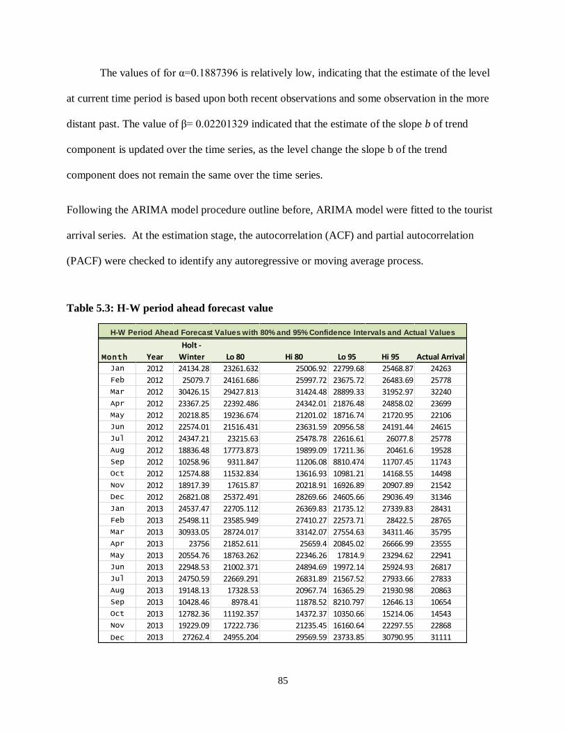
85
The values of for α=0.1887396 is relatively low, indicating that the estimate of the level
at current time period is based upon both recent observations and some observation in the more
distant past. The value of β= 0.02201329 indicated that the estimate of the slope b of trend
component is updated over the time series, as the level change the slope b of the trend
component does not remain the same over the time series.
Following the ARIMA model procedure outline before, ARIMA model were fitted to the tourist
arrival series. At the estimation stage, the autocorrelation (ACF) and partial autocorrelation
(PACF) were checked to identify any autoregressive or moving average process.
Table 5.3: H-W period ahead forecast value
Month Year
Holt -
Winter Lo 80 Hi 80 Lo 95 Hi 95 Actual Arrival
Jan 2012 24134.28 23261.632 25006.92 22799.68 25468.87 24263
Feb 2012 25079.7 24161.686 25997.72 23675.72 26483.69 25778
Mar 2012 30426.15 29427.813 31424.48 28899.33 31952.97 32240
Apr 2012 23367.25 22392.486 24342.01 21876.48 24858.02 23699
May 2012 20218.85 19236.674 21201.02 18716.74 21720.95 22106
Jun 2012 22574.01 21516.431 23631.59 20956.58 24191.44 24615
Jul 2012 24347.21 23215.63 25478.78 22616.61 26077.8 25778
Aug 2012 18836.48 17773.873 19899.09 17211.36 20461.6 19528
Sep 2012 10258.96 9311.847 11206.08 8810.474 11707.45 11743
Oct 2012 12574.88 11532.834 13616.93 10981.21 14168.55 14498
Nov 2012 18917.39 17615.87 20218.91 16926.89 20907.89 21542
Dec 2012 26821.08 25372.491 28269.66 24605.66 29036.49 31346
Jan 2013 24537.47 22705.112 26369.83 21735.12 27339.83 28431
Feb 2013 25498.11 23585.949 27410.27 22573.71 28422.5 28765
Mar 2013 30933.05 28724.017 33142.07 27554.63 34311.46 35795
Apr 2013 23756 21852.611 25659.4 20845.02 26666.99 23555
May 2013 20554.76 18763.262 22346.26 17814.9 23294.62 22941
Jun 2013 22948.53 21002.371 24894.69 19972.14 25924.93 26817
Jul 2013 24750.59 22669.291 26831.89 21567.52 27933.66 27833
Aug 2013 19148.13 17328.53 20967.74 16365.29 21930.98 20863
Sep 2013 10428.46 8978.41 11878.52 8210.797 12646.13 10654
Oct 2013 12782.36 11192.357 14372.37 10350.66 15214.06 14543
Nov 2013 19229.09 17222.736 21235.45 16160.64 22297.55 22868
Dec 2013 27262.4 24955.204 29569.59 23733.85 30790.95 31111
H-W Period Ahead Forecast Values with 80% and 95% Confidence Intervals and Actual Values

86
Figure 5.7: Forecasts fr om Holt-Winter
Figure 5.8: Holt-Winter residual plot

87
Figure 5.9: ACF of the seasonal
Figure 5.10: Seasonal ARIMA residual plots of tourist arrivals in Belize
Since the correlogram shows that one of the sample autocorrelations for lags 1-20 exceed
the significance bounds, and the p-value for the Ljung-Box test is 0.7755, we can conclude that
there is very little evidence for non-zero autocorrelations in the forecast errors up to lag 20 as
shown in Figure 5-13. The spike in the plot suggests that the model can be slightly improved

88
although it is unlikely to make much difference to the resulting forecast in Table 5-3. The
forecasted tourists’ arrival for the year 2012-2013 is presented in Table 5-3 along with the 80%
and 90% confidence interval. When compare with the actual observed arrivals it appears that the
model fits the data very well as seen in Figure 5-13.
The best fitted model was ARIMA(1,0,1)(2,1,1)(12) . This can be written as
(1 − ∅1𝐵)(1 − Φ1𝐵12 −Φ2𝐵
24)(1 − 𝐵12)𝑋𝑡 = (1 + θ1𝐵)(1 + Θ1𝐵12)휀𝑡 (5-15)
Substituting the estimated ARIMA coefficients,
(1 − 0.9744𝐵)(1 + 0.0982𝐵12 − 0.016𝐵24)(1 − 𝐵12)𝑋𝑡
= (1 − 0.7394𝐵)(1 − 0.5240𝐵12) (5-16)
Simplifying it, we get
𝑋𝑡 −휀𝑡 =0.9744𝑋𝑡−1+ 0.9018𝑋𝑡−12− 0.87871392𝑋𝑡−13+ 0.1088𝑋𝑡−24
−0.10601472𝑋𝑡−25− 0.0106𝑋𝑡−36+ 0.01032864𝑋𝑡−37
−0.7394휀𝑡− 0.524휀𝑡−12+ 038474휀𝑡−13 (5-17)
The mathematical form of the one step ahead forecasting model for Belize is given by,
𝑋𝑡 =0.9744𝑋𝑡−1 + 0.9018𝑋𝑡−12 − 0.87871392𝑋𝑡−13 + 0.1088𝑋𝑡−24
−0.10601472𝑋𝑡−25 − 0.0106𝑋𝑡−36 + 0.01032864𝑋𝑡−37
−0.7394휀𝑡 − 0.524휀𝑡−12 + 038474휀𝑡−13 (5-18)
which is different from the model forecasted by United Nation in their 1992 report on Belize.

89
Table 5.4: ARIMA model Ahead Forecast Values
Figure 5.11: Forecast from ARIMA(1.0,1)(2,1,1)12
Month Year
Forecast
ARIMA Lo 80 Hi 80 Lo 95 Hi 95 Actual Arrival
Jan 2012 24167.21 22269.83 26226.25 21326.48486 27386.323 24263
Feb 2012 25170.65 23142.89 27376.05 22136.45332 28620.714 25778
Mar 2012 30441.89 27931.85 33177.46 26688.01854 34723.744 32240
Apr 2012 23014.71 21076.73 25130.89 20117.79448 26328.782 23699
May 2012 20176.62 18444.8 22071.03 17589.05302 23144.86 22106
Jun 2012 22443.83 20483.46 24591.82 19516.00154 25810.896 24615
Jul 2012 24208.86 22060.21 26566.76 21001.09798 27906.558 25778
Aug 2012 18870.72 17171.05 20738.62 16334.17798 21801.15 19528
Sep 2012 10133.61 9208.442 11151.73 8753.387086 11731.467 11743
Oct 2012 12385.75 11240.75 13647.4 10678.10861 14366.494 14498
Nov 2012 18544.47 16810.18 20457.71 15958.74127 21549.158 21542
Dec 2012 26446.13 23946.2 29207.07 22719.95745 30783.435 31346
Jan 2013 24405.43 21881.61 27220.35 20653.02341 28839.637 28431
Feb 2013 25324.36 22658.67 28303.65 21363.0698 30020.177 28765
Mar 2013 30584.27 27312.26 34248.26 25724.34246 36362.344 35795
Apr 2013 23364.41 20827.32 26210.57 19597.74916 27855.034 23555
May 2013 20297.22 18062.77 22808.08 16981.2997 24260.651 22941
Jun 2013 22609.63 20088.95 25446.59 18870.42197 27089.785 26817
Jul 2013 24440.89 21684.02 27548.27 20352.82496 29350.093 27833
Aug 2013 18931 16772.38 21367.43 15731.17986 22781.68 20863
Sep 2013 10205.07 9029.678 11533.45 8463.296213 12305.296 10654
Oct 2013 12472.76 11022.7 14113.56 10324.63432 15067.811 14543
Nov 2013 18763.26 16562.84 21256.01 15504.47545 22706.988 22868
Dec 2013 26748.03 23585.68 30334.35 22065.92848 32423.605 31111
ARIMA Period Ahead Forecast Values with 80% and 95% Confidence Intervals and Actual Values

90
Conclusion
Tourism in Belize and the Central America region underpin their fragile economies. With
planning being an important aspect in tourism, the importance of forecasting cannot be
overemphasized. Yet, little has been done on this issue. We have developed two models. The
estimated models were subjected to validation process based on their statistical properties and
forecasting capability. The ex post forecast shows that the ARIMA(1,0,1)(2,1,1)(12) scheme provides
excellent short term forecast and the Holt-Winter also provides excellent forecasts. Of the two models
however, based on MAPE and RMSE in Table 5-1 the results shows that the Holt-Winter
Exponential smoothing model was the best for forecasting tourist arrival in Belize. The model
does not show how various socioeconomic variables affect the number of arrivals. If such
information is needed, a structural model should be developed and its simulation capability
should be examined. Since the development of structural model can be costly, the benefit of
additional information that would be obtained should be weighed against the costs of obtaining
them.
The ARIMA models deal with seasonality in a more implicit manner--we can't easily see in
the ARIMA output how the average for January, say, differs from the average for June.
Depending on whether it is deemed important to isolate the seasonal pattern, this might be a
factor in choosing among models. The ARIMA models have the advantage that, once they have
been initialized, they have fewer "moving parts" than the exponential smoothing and adjustment
models and as such they may be less likely to over fit the data. ARIMA models also have a more
solid underlying theory with respect to the calculation of confidence intervals for longer-horizon
forecasts than do the other models.

91
Chapter 6: Future Research
We proposed in developing a statistical economic model that drives the economy of Belize.
This is extremely important because no such model does exist. The process, by which we will
proceed in developing this model, is first identifying the attributable variables that drive the
economy, such as agriculture, tourism, temperature and rainfall etc. with our model response
variable which would be the value return base on the attributable variables. Most importantly, we
will identify the interactions that would be involved in the modeling process and once we have
identified it, we believe we can developed a very good model and validate it to be used by my
country Belize.
Usefulness of such model is that it can estimate it potential economic behavior, secondly it
identifies the significant attributable variables that drives the economy, thirdly it will identify the
interaction of the risk variables that drives the economy ,fourthly , we can use the modelling
aspect to rank the attributable variables base on their percentage of contribution to the economy
which is useful to government will know what entities they should focus in in order to increase
the overall economy. Finally we will proceed perform surface response analysis that is we want
to be within 95% certainly, what are the values of the attributable variables that drives the model
that maximize the economy. This is extremely important because this information to the
government in the sense that they can try to maintain the values that will maximize the economy.
For example, if tourism is one of the key factors then they should aim to maintain the optimum
values.
Belize has a significant need for developing a statistical model that drives the tourism
sector. Since tourism is one on the key factors that drives the economy. In which our response
variable will be tourism arrivals and the attributable variables mentioned in the previous

92
proposed research. Since we know from descriptive statistics, that tourism is one of the key
factors in driving Belize’s economy. Having such a model is useful because we will able to
identify the key factors that drive the tourism sectors.
As a result of the present study, we will continue the research on the subject area by
studying the following problems. Investigate the selection of the best ARIMA model utilizing
AIC versus BIC with respect to small, medium and large sample sizes. Overall, the results
enable forecasters to choose the most suitable model, based on the available data, forecast
horizon for forecasting tourism demand. A future research would aim at revisiting the
robustness of our results in multivariate nonlinear frameworks, which controls for additional
exogenous variables that affect tourism demand. Another area of interest is to examine whether a
combination of forecasts based on the aforementioned models provides any additional gains in
the forecasting accuracy of tourism demand in Belize.
While good research finding have been obtained, further work needs to be done to
generalize the finding to other neighboring countries with similar characteristics. Future studies
can employ the same forecasting model but with different data series for forecasting accuracy
validity.

93
References
Adiku, S., Dayananda, P., Rose, C., & Dowuona, G. (1997). Analysis of within-season rainfall
characteristics and simulation of daily rainfall in two Savannah Zones in Ghana.
Agriculture Forest Meteorology, 86 (96), 51-62 ; 168-1923; 14-8.
Aksoy, H. (2000). Use of Gamma Distribution in Hydrological Analysis. Turkey Journal of
Engineering Evironmental Science, 24, 419-428.
Amemiya, T. (1985). Advanced Econometrics. Cambridge, Mass.: Harvard University Press.
Amihud, Y. B. (1992). Further evidence in the risk-relationship. Working Paper No. S-93-11.
Archer, B. (1987). Demand forecasting and estimation. In J. Ritchie, & C. Goeldner, Travel
Tourism and Hospitality Research (pp. 77-85). New York: Wiley.
Bails, D., & Peppers, L. (1993). Business fluctuations-forecasting techniques and applications.
New Jersey: Prentice-Hall International.
Bansal, R. D. (1993). A new approach to international arbitrage pricing. Journal of Finance 48,
1719-1747.
Bansal, R. S. (1993). The Conditional CAPM and the Cross-Section of Expected Returns 51, No
arbitrage and arbitrage pricing: A new approach. Journal of Finance 48, 1231-1262.
Banz, R. W. (1981). The relationship between return an dmarket value of common stocks.
Journal of Financial Economics 9, 3-18.
Basu, S. ( 1983). The relationship between earnings yield, market value, and return for NYSE
common stocks: Further evidence. Journal of Financial Economics 12, 51-74.
Bates, J., & Granger, C. (1969). The combination of forecasts. Operation Research Quarterly, 20
, 451-468.
Beaulieu, J., & Miron, J. (1993). Seasonal unit roots in aggregate US data. Journal of
Econometrics 55 (1-2), 305-328.
Berk, J. B. (1995). A critique of sized-related anomalies. Review of Financial Studies 8, 275-286.
Bernanke, B. S. (1990). On the predictive power of interest rates and intererst rate spreads. New
England Economic Review, 51-68.

94
Bhandari, L. C. (1988). Debtlequity ratio and expected common stock returns: Empirical
Evidence. Journal of Finance 43, 507-528.
Black, & Fischer. (1972). Capital market eqilibrium with restricted borrowing. Journal of
Business 45, 444-455.
Black, & Fischer. (1993). Beta and Return. Journal of Portfolio Management 20, 8-18.
Black, F. M. (1972). The capital asset pricing model: Some emipirical tests. New York: Praeger.
Black, F. M., & Scholes, M. (1972). The Capital Asset Pricing Model: Some Empirical Tests, pp
79-121. New York: Praeger Publishers.
Black, F., Michael C. Jensen, & Scholes, M. (1972). The Capital Asset Pricing Model: Some
Empirical Tests, pp 79-121. New York: Praeger Publishers.
Board, S. T. (n.d.). Annual Statistical Report on visitor arrivals to Singapore. Various Issues.
Bodurtha, J. N., & Mark, N. C. (1991). Testing the CAPM with time-varying risks and returns.
Journal of Finance 46, 1485-1505.
Bollerslev, T. R. (1988). A capital asset pricing model with time varying covariances. Journal of
Political Economy 96, 116-131.
Bossaerts, P. (1994). Time series analysis of inefficient financial markets. Manuscript,
California Institute of Technology.
Box, G., & Jenkins, G. (1976). Time series analysis, forecasting and control. San Francisco:
Holden Day.
Box, G., & Jenkins, G. (1976). Times Series Analysis: Forecasting and Control. San Francisco:
Holden Day.
Breen, W. J. (1989). Economic significance of predictable variations in stock index returns.
Journal of Finance 44, 1177-1190.
Breen, W. J. (1994). On selection biases in book-to-market based tests of asset pricing models.
Working Paper No. 167.
Brigham, E. C. (2005). Financial Management: Theory and Practice, 11th Edition. South-
Western.
Bureau, T. (2008). Report on Air Travel Statistics. Taiwan, R.O.C: Tourism Bureau, MOTC.
Campbell, J. Y. (1993). Intertemporal risk and returns. Working Paper No. 4554 .
Carhart, M. M. (1995). Testing the conditional CAPM. Manuscript, University of Chicago.

95
Chan, K. N.-f. (1985). An exploratory investigation of the firm size effect. Journal of Financial
Economics 14, 451-471.
Chan, K. N.-f. (1988). An unconditional asset-pricing test and the role of firm size as an
instrumental variable for risk. Journal of Finance 43, 309-325.
Chan, L. K. (1993). Are the reports of beta's death premature? Journal of Portfolio Management
19, 51-62.
Chan, L. K. (1995). Evaluating the performance of value versus glamour stocks: The impact of
selection bias. Journal of Financial Economics 38, 269-296.
Chan, Y. (1993). Forecasting Tourism: a sine wave time series regression approach. Journal of
Travel Research, 31, 58-60.
Chari, V. V. (1986). Seasonalities in security returns: The case of earnings announcements.
Journal Financial Economics 21, 101-122.
Chawarit, W. (2000). "The Comparison of CAPM and APT in described return of stock
predicting" .
Chen, N.-F. (1991). Financial investment oppotunities and the macroeconomy. Journal of
Finance 46, 529-554.
Chen, N.-F. R. (1986). Economic forces and the stock market. Journal of Business, 383-404.
Cho, H., Bowman, K., & North, G. (2004). A comparison of Gamma and Log-normal
distributions for characterizing satellite rain rates from the tropical rainfall measuring
mission. Journal of Applied meteorology, 43 (165), 1586-1597 [3].
Choy, D. (1984). Forecasting tourism revisited. Tourism Management 5 (3), 171-176.
Chu, F. (1998). Forecasting tourism arrivals: nonlinear sine wave or ARIMA? Journal of Travel
Research, 36, 79-84.
Chu, F. (1998). Forecasting tourism demand in Asian - Pacific countries. Annual of Tourism
Research 25 (3), 597-615.
Chu, F. (2004). Forecasting tourism demand: A cubic polynomial approach. Tourism
Management 25 (2), 209-218.
Cochrane, J. H. (1992). A cross-sectional test of a production based asset pricing model.
Working Paper No. 4025 NBER.
Connor, G. R. (1988). The arbitrage pricing theory and multi-factor models of asset returns.
Journal of Finance.

96
Connor, G. R. (1988a). Risk and return in an equlibrium APT: Application of a new test
methodology. Journal of Financial Economics 21, 255-289.
Connor, G., & Sehgal, S. (2001). Tests of the Fama and French Model in India.
Coshall, J. (2006). Time series analysis of UK outbound travel by air. Journal of Travel
Research 44 (3), 335-347.
Crouch, I. (1994). The study of international tourism demand: a survey of practice. Travel
Research, 32, 41-55.
Dan'azumi, S., Shamsudin, S., & Aris, A. (2010). Modeling the Distribution of Rainfall Intensity
using Hourly Data. American Journal of Environmental Sciences, 6 (3), 238-243.
Daniel, K. S. (1995). Evidence on the characteristics of cross sectional variation in stock returns.
Manuscript, University of Chicago.
Das, P., Subash, N., Sikka, A., Sharda, V., & Sharma, N. (2006). Modeling weekly rainfall using
gamma probability distribution and Markov chain for crop planning in a sub-humid(dry)
climate of central Biar. Indian Journal of Agricultural Science, 76 , 358-361.
Davis, J. L. (1994). The cross-section of realized stock returns: The pre-COMPUSTAT evidence.
Journal of Finance 49, 1579-1593.
Deng, J. (1982). Control problems of grey systems. Systems and Control Letters 1 (1), 288-294.
Dharmaratne, G. (1995). Forecastinf tourist arrival in Barbados. Annual of Tourism Research 22
(4), 804-818.
Diaz-Gimenez, J., Prescott, E. C., Fitzgerald, T., & Alvarez, F. (1992). Banking in computable
general equilibrium economics. Journal of Economic Dynamics and Control 16, 533-559.
Dickey, D., & Fuller, W. (1979). Distribution of the estimators for autoregressive time series
with a unit root. Journal of the American Statistical Association 74 (366), 427-431.
Dybvig, P., & Jr., J. I. (1982). Mean-variance theory in capital markets. Journal of Business 55,
233-251.
Dybvig, P., & Ross, S. A. (1985). Differential information and performance measurement using
a security market line. Journal of Finance 40, 383-400.
Eadington, W., & Redman, M. (1991). Economics and Tourism. Tourism Research, 18, 41-56.
Ediger, V., & Kar, S. (2007). ARIMA forecasting of primary energy demand by fuel in Turkey.
Energy Policy 35 (3), 1701-1708.
97
Eli, A., Shaffie, M., & Wan Zin, W. (2012). Preliminary study on bayesian extreme rainfall
analysis: A case study of Alor Setar, Kedah, Malaysia. Sains Malaysiana, 41 (11), 1403-
1410.
Espassa, A. (1994). Comment on "Time series analysis, forecasting and econometric meodeling:
the structural econometric modeling, time series analysis appraoch". Journal of
Forecasting 13 (2), 235-239.
Fadhilah, Y., Zalina, M., Nguyen, V., Suhaila, S., & Zulkifli, Y. (2007). Fitting the Best-Fit
Distribution for the Hourly Rainfall Amonunt in the Wilayah Persekutuan. Jurnal
Teknologi, 46 (C), 49-58.
Fama, E. F. (1968). Return and Equilibrium : Some Clarifying Comments. Journal of Finance
Vol.23 No.1, 29-40.
Fama, E. F., & French, K. (June 1992). The Cross-Section of Expected Stock Returns. Journal of
Finance, 427-466.
Fama, E. F., & French, K. R. (1989). Business conditions and the expected returns on bonds and
stocks. Journal of Financial Economics 25, 23-50.
Fama, E. F., & French, k. R. (1992). The cross-section of expected stock returns. Journal of
Finance 47, 427-466.
Fama, E. F., & French, K. R. (1993). Common risk factors in the returns of bonds and stocks.
Journal of Financial Economics 33, 3-56.
Fama, E. F., & MacBeth, J. D. (1973). Risk, Return and Equilibrium: Empirical tests. Journal of
Political Economy 81, 607-636.
Fama, E. F., & Schwert, G. W. (1977). Human capital and capital market equilibrium. Journal of
Financial Economics 4, 115-146.
Fama, E., & French, K. (1992). The Cross-Section of Expected Stock Returns. Journal of
Finance 47, 427-465.
Fama, E., & French, K. (1993). Common Risk Factors in the Returns on Stocks and Bonds.
Journal of Financial Economics 33, 3-56.
Fama, E., & French, K. (1996). Multifactor Explanations of Asset Pricing Anomalies. Journal of
Finance 51, 55-84.
Fama, E., & French, K. (1998). Value versus Growth : The International Evidence. Journal of
Finance 53, 1975-1999.
Fama, E., & French, K. (2004). The Capital Asset Pricing Model : Theory and Evidence.

98
Ferson, W. E., & Foerster, S. (1994). Finite sample properties of the generalized method of
momemts in tests of conditional asset pricing models. Journal of Financial Economics
36, 39-35.
Ferson, W. E., & Harvey, C. R. (1991). The variation of economic risk premiums. Journal of
Political Economy 99, 385-415.
Ferson, W. E., & Harvey, C. R. (1993). The risk and predictability of international equity returns.
Review of Financial Studies 6 (3), 527-566.
Ferson, W. E., & Korajczyk, R. A. (1993). Do arbitrage pricing models explain the predictability
of stock returns? Working Paper, Kellogg Graduate School of Management, Northwestrn
University.
Fildes, R. (1989). Evaluation of aggregated and individual forecast method selection rules.
Management Science 35 (9), 1056-1065.
Franses, P. (1991). Seasonality, nonstationary and the forecasting of monthly time series.
International Journal of Forecasting 7 (2), 199-208.
Franses, P., & Hobijn, B. (1997). Critical values for unit root tests in seasonal time series.
Journal of Applied Statistics 24 (1), 25-48.
French, C. W. ( December 2002). Jack Treynor's 'Toward a Theory of Market Value of Risky
Assets'.
French, C. W. (2003). The Treynor Capital Asset Pricing Model. Journal of Investment
Management, Vol.1 No. 2, 60-72.
Gibbons, M. R. (1982). Multivariate tests of financial models: A new approach. Journal of
Financial Economics 10, 3-27.
Greenwood, J., Landwehr, J., & Matalas, N. (1979). Probability weighted moments: definition
and relation to parameters of several distributions expressible in inverse form. Water
Resource Research, 15, 1049-1054.
Hansen, L. P. (1982). Large sample properties of generalized method of moment estimators.
Econometrica 50, 1029-1054.
Hansen, L. P., & Jagannathan, R. (1991). Implications of security market data for models of
dynamic economics. Journal of Political Economy 99, 225-262.
Hansen, L. P., & Jagannathan, R. (1994). Assessing specification errors in stochastic discount
factor models. Technical Working Paper No. 153 NBER.

99
Hansen, L. P., & Richard, S. F. (1987). The role of conditioning information in deducting
testable restrictions implied by dynamic asset pricing models. Econometrica 55, 587-613.
Hansen, L. P., & Singleton, K. (1982). Generalized instrumental variables estimation in
nonlinear rational expectation models. Econometrica 50, 1269-1286.
Hanson, L., & Vogel, R. (2008). The Probability Distribution of Daily Rainfall in the United
States. World Environment and Water, 1-12.
Harvey, A. (1981). Time Series Models. Deddington: Philip Allan.
Harvey, C. R. (1989). Time-varying conditional covariances in tests of asset pricing models.
Journal of Financial Economics 24, 289-318.
Hosking, J. (1990). L-Moments: Analysis and stimation of distribution using linear combinations
of order statistics. Journal Research Statistic Society B., 52 (1), 105-124.
Hosking, J. (1991). Fortran routines for use with method of L-moments, Version 2, Res. Rep. RC
17079. York-Town Heights, NY 10598: IBM Research Division.
Hosking, J. (2000). Research Report Fortran Routines for use with method of L- moments,
Version 3.03. New York, 33: IBM Research Division.
Hosking, J., & Wallis, J. (1997). Regional Frequency Analysis. New York, 224: Cambridge
University Press.
Houghton, J. (1978). Birth of a Parent: The Wakeby distribution for modeling flood flows. Water
Resources Research, 14 (6), 1105-1109.
Hylleberg, S. e. (1990). Seasonal integration and cointegration. Journal of Econometrics 44 (2),
215-238.
Jagannathan, R., & Wang, Z. (1993). The CAPM is alive and well. Staff Report 165, Reserve
Bank of Minneapolis.
Jagannathan, R., & Wang, Z. (September 13-15, 1992). The cross-section of expected stock
returns: Do size and book to market equity measure systematic risk better than beta? .
Notes for the Berkeley Program in Finance on "Are Betas Irrelevant? Evidence and
Implecations for Assest Management".
Janteeratikun, N. (2000). The Testing of CAPM by factor analysis method: A Case study of the
StockExchanfe of Thailand.
Jegadeesh, N. (1992). Does market risk really explain the size effects? Journal of Financial and
Quantitative Analysis 27, 337-351.

100
Kandel, S., & Stambaugh, R. F. (1987). On correlations and inferences about meanvariance
efficiency. Journal of Financial Economics 18, 61-90.
Kandel, S., & Stambaugh, R. F. (1990). A mean-variance framework for tests of asset pricing
models. Review of Financial Studies 2, 125-156.
Kandel, S., & Stambaugh, R. F. (1995). Portfolio innefficiency and the cross-section of expected
returns. Journal of Finance 50, 157-184.
Kedem, B., Pavlopoulos, H., Guan, X., & Short, D. (1994). Probability distribution model for
Rain rate. Journal of Applied Meteorology, 33 , 486-1493 ; 1520-0450.
Keim, D. B., & Stambaugh, R. F. (1986). Predicting returns in the stock and bond markets.
Joural of Financial Economics 17, 357-390.
Khan, H., Phang, S., & Toh, R. (1996). Tourism growth in Singapore: An optimal target.
Tourism Research, 23, 222-223.
Kim, J., & Moosa, I. (2005). Forecasting international tourist flows to Australia: a comparison
between the direct and indirect methods. Tourism Management 26 (1).
Kim, S., & Song, H. (1998). Analysis of tourism demand in South Korea: a cointegration and
error correction approach. Tourism Analysis 3 (1), 25-41.
Koc, E., & Altinay, G. (2007). An analysis of seasonality in monthly per person tourist spending
in Turkish inbound tourism from a market segmentation perspective. Tourism
Management 28 (1), 227-237.
Kothari, S., Shanken, J., & Sloan, R. G. (1995). Another look at the cross-section of expected
stock returns. Journal of Financial 50, 185-224.
Kulendran, N., & Witt, S. (2001). Cointegration versus least squares regression. Annual of
Tourism Research 28 (2), 291-311.
Kulendran, N., & Witt, S. (2003). Forecasting the demand for international business tourism.
Journal of Travel Research 41 (3), 265-271.
Kulendran, N., & Wong, K. (2005). Modeling seasonality in tourism forecasting. Journal of
Travel Research 44 (2), 163-170.
Landwehr, J., Matalas, N., & Wallis, J. (1979a). Probability weighted moments compred with
some traditional techniques in estimating Gumbel Parameters and Quarterlies. water
Resources Research15 (5), 1055-1065.

101
Landwehr, J., Matalas, N., & Wallis, J. (1979b). Estimation of parameters and qualities of
Wakeby distributions 1. known lower bounds. Water Resources Research, 15 (6), 1361-
1372.
Landwehr, J., Matalas, N., & Wallis, R. (1979a). Estimation of parameters an qualitites of
Wakeby distributions 1. known lower bounds. Water Resources Research, 15 (6), 1361-
1372.
Landwehr, J., Matalas, N., & Willis, J. (1978). Some comparisons of flood statistics in real and
logspace. Water Resource Research, 14 (5), 902-920.
Lehmann, B. N., & Modest, D. M. (1988). The empirical foundations of the arbitrage pricing
theory. Journal of Financial Economics 21, 213-254.
Lewis, C. (1982). International and business forecxasting methods. London: Butterworths.
Lim, C. M. (1999). A seasonal analysis of Malaysian tourist arrivals to Australia. Mathematics
and Computers in Simulation 48 (6), 573-583.
Lim, C., & McAleer, M. (2000). A seasonal analysis of Asian tourist arrivals to Australia.
Applied Econometrics 32 (4), 499-509.
Lim, C., & McAleer, M. (2002). Time series forecasts of international travel demand for
Australia. Tourism Management 23 (4), 389-396.
Lim, C., & Pan, G. (2005). Inbound tourism developpments and patterns in China. Mathematics
and Computers in Simulation 68 (6), 499-507.
Ling, W., & Ismail, N. (2012). Analysis of T-Year Return Level for Partial Duration Rainfall
Data. Sains Malaysiana, 41 (11), 1389-1401.
Lintner, J. (1965). Security Prices, Risk and Maximal Gains from Diversification. Journal of
Finance 20, 587-615.
Lintner, J. (1965). The valuation of risk assets and the selection of risky investments in stock
portfolio and capital budgets. Review of Economics and Statistics 47, 13-37.
Lintner, J. (1965). The valuation of risk assets and the selection of risky investments in stock
portfolios and capital budgets. Review of Economics and Statistics 47 (1), 13-37.
Liung, G., & Box, G. (1978). On a measure of lack of fit in time series models. Biometrika 65
(2), 297-303.
Long, J. (1974). Stock prices, inflation, and the term structure of interest rates. Journal of
Financial Economics 1, 131-170.

102
Makridakis, S., & Hibon, M. (1979). Accuracy of Forecasting: an empirical investigation.
Journal of the Royal Statistical Society Series a, 142 (2), 97-125.
Makridakis, S., Wheelwright, S., & Hyndman, R. (1998). Forecasting: methods and
applications. New York: John Wiley & Sons.
Mandelker, G. (1974). Risk and Return: The case of merging firms. Journal of Financial
Economics 4, 303-335.
Markowitz, H. M. (1999). The early history of protfolio theory : 1600-1960. Financial Analysts
Journal Vol.55 No. 4.
Matalas, N., Slack, J., & Wallis, J. (1975). Regional skew in search of a parent. Water Resources
Research, 11 (6), 815-826.
Mayers, D. (1972). Nonmarkable assets and capital market equilibrium under uncertainty. New
York: Praeger.
McCullagh, P., & Nelder, J. (1989). Generalized Linear Models, 2nd Edition. London: Chapman
and Hall.
Mehrling, P. (2005). Fischer Black and the Revolutionary Idea of Finance. Hoboken: John
Wiley & Sons, Inc.
Merton, R. C. (1973). An intertemporal capital asset pricing model. Ecomometrica 41, 867-887.
Merton, R. C. (1980). On estimating the expected return on the market: An exploratory
investigation. Journal of Financial Economics 8, 323-361.
Modarres, R. (2006). Regional Precipitation Climates of Iran. Journal of Hydrology (NZ), 45 (1),
13-27.
Mossin, J. (1966). Equilibrium in a Capital Asset Market. Econometric 34, 768-783.
Mossin, J. (1966). Equilibrium in a Captial Asset Market. Econometrica Vol.34 No. 4, 768-783.
Mullins, D. W. (January-February 1982). Does the capital asset pricing model work? Harvard
Business Review, 105-113.
Organization, W. T. (1994). Current Trend and Tourism . WTO - Madrid.
Palm, F., & Zellner, A. (1992). To compare or not to combine? Issues of combining forecasts.
JOurnal of Forecasting 11 (8), 687-701.
Pankratz, A. (1983). Forecasting with univariate Box-Jenkins models: concepts and cases. New
York: Wiley.

103
Park, J., & Jeon, J. (2000). Maximum likelihood estimation of Wakeby distribution. Technical
Report, Department of Statistics, Chonnam N University, Kwangju, Korea.
Park, J., Kim, R., & Jung, H. (2000). Parameter Estimations of Waked Distribution and it's
Application to Korean Extreme Rainfall. The Tenth Japan and Korea Joint Conference of
Statistics, Beppu, Japan.
Rao, A., & Hamed, K. (2012). Flood Frequency Analysis. United States, 2000.
Reinganum, M. R. (1981). Misspecification of capital asset pricing: Empirical anomalies based
on earnings yields and market values. Journal of Financial Economics 9, 19-46.
Roll, R. (1977). A critique of the asset pricing theory's test; part 1: On past and potential
testability of the theory. Journal of Financial Economics 4, 129-176.
Ross, S. (1976). The Arbitrage Pricing Theory of Capital Asset Pricing. Journal of Economic
Theory 13, 341-360.
Ross, S. (2004). Introduction to Probability and Statistics for Engineers and Scientists, 3rd
Edition. London: Elsevier Academic Press.
Ross, S. A. (1976). The arbitrage theory of capital asset pricing. Journal of Economic Theory 13,
341-360.
Ross, S. A. (1977). The Capital Asset Pricing Model (CAPM), Short-sale Restrictions and
Related Issues. Journal of Finance 32, 177.
Rubinstein, M. (2006). A History of the Theory of Investments. Hoboken: John Wiley & Sons,
Inc.
Salisu, D., Supiah, S., & Azmi, A. (2010). Modeling the Distribution of Rainfall Intensity using
Hourly Data. American Journal of Environmental Sciences, 6 (3), 238-243.
Shanken, J. (1985). Multivariate tests of the zero-beta CAPM. Journal of Financial Economics
14, 327-348.
Shanken, J. (1987). Multivariate proxies and asset pricing relations: Living with the roll critique.
Journal of Financial Economics 18, 91-110.
Shanken, J. (1992). On the estimation of beta-pricing models. Review of Financial Studies 5, 1-
33.
Sharma, M., & J., B. S. (2010). Use of Probability Distribution in Rainfall Analysis. New York
Science Journal, 3 (9), 40-49.
104
Sharpe, W. (1964). Capital Asset Prices: A Theory of Market Equilibrium under Condition of
Risk. Journal of Finance 19, 425-442.
Sharpe, W. F. (1964). Capital asset prices: A thoery of market equilibrium under conditions of
risk. Journal of Finance 19, 425-442.
Sharpe, W. F. (1964). Capital Assets Prices: A theory of market eqilibrium under conditions of
risk. Journal of Finance 19, (3), 425-442.
Simolo, C., Brunetti, M., Maugeri, M., & Nanni, T. (1992). Improving estimation of missing
values in daily precipitation data by a probability density function-preserving approach.
International Journal of Climatol DOI:10.1002/joc.
Song, H., & Wang, K. (2003). Tourism demand modelling: a time varying parameter approach.
Journal of Travel Research 42 (1), 57-64.
Srikanthan, R. (July 13-17, 2009). A multisite daily rainfall data generation model for climate
change conditions. 18th World IMACS/MODSIM Congress, Cairns, Australia.
Stambaugh, R. F. (1981). Missing assests, measuring the market, and testing the capital asset
pricing model. Doctoral dissertation, University of Chicago.
Stambaugh, R. F. (1982). On the exclusion of assets from tests of the teo-parameter model: A
sensitivity analysis. Journal of Financial Economics 10, 237-268.
Stock, J., & Watson, M. (1989). New indexes of coincident and leading economic indicators.
Olivier J. Blanchard ; Stanley Fischer Eds.: NBER Macroeconomics Annual.
Stone, B. K. (1970). Risk, Return, and Equilibrium: A General Single-Period Theory of Asset
Selection and Captial-Market Equilibrium. Cambridge: MIT Press.
Suhaila, J., & Jemain, A. (2007a). Fitting the Statistical Distributions to the Daily Rainfall
Amount in Peninsular Malaysia. Jurnal Teknologi, 46 (C), 33-48.
Suhaila, J., & Jemain, A. (2007b). Fitting daily rainfall amount in Malaysia using the normal
transform distribution. Journal of Applied Sciences, 7 (14), 1880-1886.
Tobin, J. (1958). Liquidity preference as behavior towards risk. The Review of Economic Studies,
25.
Treynor, J. L. (1961). Market Value, Time, and Risk.
Treynor, J. L. (1962). Toward Theory of Market Value of Risky Assets. London: Risk Books.
Tseng, F., Yu, H., & Tzeng, G. (2001). Applied hybrid grey model to forecast seasonal time
series. Technological Forecasting and Social Change, 67 (2), 291-302.

105
Uysal, M., & Crompton, J. (1985). An overview of approaches used to forecast tourism demand.
Journal of Travel and Research, 23, 7-15.
Van Doorn, J. (1984). Tourism forecasting and policymaker-criteria of usefulness. Tourism
Management, (1), 24-39.
Wan Zin, W., & Jemain, A. (2009). The best fitting distributionof annual maximum rainfall in
Peninsular Malaysia based onmethods of L-moment nad LQ-moment. Theory Application
in Climatiol, 96, 337-344.
Wang, C. (2004). Predicting tourism demand using fuzzy time series and hybrid grey theory.
Tourism Management, 25 (3), 367-374.
Wilks, D. (1992). Adopting stochastic weather generation algorithms for climate change studies.
Climate Change, 22 , 67-84.
Wilks, D. (1993). Comparison of three-parameter probability distribution for representing annual
extreme and partial duration precipitation series. Water Resources Research, 29 (10),
3543-3549.
Winters, P. (1960). Forecasting sales by exponentially weighted moving averages. Management
Science, 6 (3), 324-342.
Witt, S., & Martin, C. (1987). Econometric models for forecasting international tourism demand.
Journal of Travel Research, 25 (3), 23-30.
Witt, S., & Witt, C. (1995). Forecasting tourism demand: a review of empirical research.
International Journal of Forecasting, 11 (3), 447-475.
Zalina, M., Amir, H. M., Desa, M. N., & Nguyen, V. (March 2002). Statistical analysis of at-site
extreme rainfall processes in Peninsular Malaysia. Regional Hydrology: Bridging the
Gap Between Research and Practice(Proceeding of the Fourth International FRIEND
Conference.
Zalina, M., Desa, M., Nguyen, V., & Kassim, A. (2002). Selecting a probability distribution for
extreme rainfall series in Malaysia. Water Science Technology, 45, 63-68.
Zellner, A., & Tobias, J. (2000). A note on aggregation, disaggregation and forecasting
performance. Journal of Finance, 19 (5), 457-465.
Zhou, G. (1994). Analytical GMM tests: Asset pricing with time-varying risk premiums. Review
of Financial Studies 7, 687-709.