Embed Size (px)
Citation preview
STATISTICAL METHODS IN FINANCE
(Preliminary version)
Dr Antoine Jacquier
Department of Mathematics
Imperial College London
Autumn Term 2019-2020
MSc in Mathematics and Finance
This version: December 5, 2019
1
Contents
1 Descriptive Statistics and Python 7
1.1 Python for Statistics . . . . . . . . . . . . . . . . . . . . . . . . . . . . . . . . . . . 7
1.1.1 A quick introduction to programming languages . . . . . . . . . . . . . . . 7
1.1.2 Statically typed languages . . . . . . . . . . . . . . . . . . . . . . . . . . . . 7
1.1.3 Interpreted languages . . . . . . . . . . . . . . . . . . . . . . . . . . . . . . 8
1.1.4 Functional and query languages . . . . . . . . . . . . . . . . . . . . . . . . . 8
1.2 Python . . . . . . . . . . . . . . . . . . . . . . . . . . . . . . . . . . . . . . . . . . 8
1.2.1 Python in Finance . . . . . . . . . . . . . . . . . . . . . . . . . . . . . . . . 8
1.2.2 General Python libraries . . . . . . . . . . . . . . . . . . . . . . . . . . . . . 8
1.2.3 Python for Economics and Finance . . . . . . . . . . . . . . . . . . . . . . . 9
1.2.4 Python libraries for plotting . . . . . . . . . . . . . . . . . . . . . . . . . . . 9
1.2.5 Python libraries for Machine learning . . . . . . . . . . . . . . . . . . . . . 9
1.3 Online data sources . . . . . . . . . . . . . . . . . . . . . . . . . . . . . . . . . . . . 9
Economics database . . . . . . . . . . . . . . . . . . . . . . . . . . . . . . . 9
Finance database . . . . . . . . . . . . . . . . . . . . . . . . . . . . . . . . . 10
Other interesting databases . . . . . . . . . . . . . . . . . . . . . . . . . . . 10
2 Applied Multivariate Statistical Analysis 11
2.1 A short introduction to Matrix algebra . . . . . . . . . . . . . . . . . . . . . . . . . 11
2.1.1 Introductory tools . . . . . . . . . . . . . . . . . . . . . . . . . . . . . . . . 11
2.1.2 Spectral Theory for matrices . . . . . . . . . . . . . . . . . . . . . . . . . . 12
2.1.3 Quadratic forms . . . . . . . . . . . . . . . . . . . . . . . . . . . . . . . . . 16
2.1.4 Derivatives . . . . . . . . . . . . . . . . . . . . . . . . . . . . . . . . . . . . 17
2.1.5 Block matrices . . . . . . . . . . . . . . . . . . . . . . . . . . . . . . . . . . 18
2.2 Essentials of probability theory . . . . . . . . . . . . . . . . . . . . . . . . . . . . . 18
2.2.1 PDF, CDF and characteristic functions . . . . . . . . . . . . . . . . . . . . 19
2.2.2 Some useful inequalities . . . . . . . . . . . . . . . . . . . . . . . . . . . . . 19
2.2.3 Gaussian distribution . . . . . . . . . . . . . . . . . . . . . . . . . . . . . . 21
2
2.2.4 Convergence of random variables . . . . . . . . . . . . . . . . . . . . . . . . 21
Convergence in distribution . . . . . . . . . . . . . . . . . . . . . . . . . . . 22
Convergence in probability . . . . . . . . . . . . . . . . . . . . . . . . . . . 23
Almost sure convergence . . . . . . . . . . . . . . . . . . . . . . . . . . . . . 23
Convergence in mean . . . . . . . . . . . . . . . . . . . . . . . . . . . . . . . 23
2.2.5 Laws of large numbers and Central Limit Theorem . . . . . . . . . . . . . . 23
2.3 Introduction to statistical tools . . . . . . . . . . . . . . . . . . . . . . . . . . . . . 24
2.3.1 Joint distributions and change of variables . . . . . . . . . . . . . . . . . . . 24
2.3.2 Mean, covariance and correlation matrices . . . . . . . . . . . . . . . . . . . 25
2.3.3 Forecasting . . . . . . . . . . . . . . . . . . . . . . . . . . . . . . . . . . . . 27
2.4 Multivariate distributions . . . . . . . . . . . . . . . . . . . . . . . . . . . . . . . . 27
2.4.1 A detailed example: the multinormal distribution . . . . . . . . . . . . . . . 27
The univariate case . . . . . . . . . . . . . . . . . . . . . . . . . . . . . . . . 27
The matrix case . . . . . . . . . . . . . . . . . . . . . . . . . . . . . . . . . 29
2.4.2 Other useful distributions . . . . . . . . . . . . . . . . . . . . . . . . . . . . 30
Chi Square Distribution . . . . . . . . . . . . . . . . . . . . . . . . . . . . . 30
Student Distribution . . . . . . . . . . . . . . . . . . . . . . . . . . . . . . . 30
Wishart distribution . . . . . . . . . . . . . . . . . . . . . . . . . . . . . . . 30
2.5 Application: Markowitz and CAPM . . . . . . . . . . . . . . . . . . . . . . . . . . 31
3 Statistical inference 33
3.1 Estimating statistical functionals . . . . . . . . . . . . . . . . . . . . . . . . . . . . 33
3.2 Statistical inference . . . . . . . . . . . . . . . . . . . . . . . . . . . . . . . . . . . . 41
3.2.1 Definition of estimators . . . . . . . . . . . . . . . . . . . . . . . . . . . . . 41
3.3 Parametric inference . . . . . . . . . . . . . . . . . . . . . . . . . . . . . . . . . . . 44
3.3.1 The method of moments . . . . . . . . . . . . . . . . . . . . . . . . . . . . . 44
3.3.2 The generalised method of moments . . . . . . . . . . . . . . . . . . . . . . 45
3.3.3 The Delta method . . . . . . . . . . . . . . . . . . . . . . . . . . . . . . . . 46
3.3.4 Maximum likelihood method . . . . . . . . . . . . . . . . . . . . . . . . . . 47
Asymptotic behaviour of the log-likelihood function . . . . . . . . . . . . . 49
Consistency of the maximum likelihood estimator . . . . . . . . . . . . . . . 49
3.3.5 Bayes estimators . . . . . . . . . . . . . . . . . . . . . . . . . . . . . . . . . 50
3.3.6 Regular statistical models . . . . . . . . . . . . . . . . . . . . . . . . . . . . 52
3.3.7 Comments about estimators and bias . . . . . . . . . . . . . . . . . . . . . 54
Stability . . . . . . . . . . . . . . . . . . . . . . . . . . . . . . . . . . . . . . 55
Parallelisation . . . . . . . . . . . . . . . . . . . . . . . . . . . . . . . . . . . 55
3.4 Hypothesis testing . . . . . . . . . . . . . . . . . . . . . . . . . . . . . . . . . . . . 55
3
3.4.1 Simple tests . . . . . . . . . . . . . . . . . . . . . . . . . . . . . . . . . . . . 56
3.4.2 Composite tests . . . . . . . . . . . . . . . . . . . . . . . . . . . . . . . . . . 58
3.4.3 Comparison of two Gaussian samples . . . . . . . . . . . . . . . . . . . . . . 60
Comparing the means . . . . . . . . . . . . . . . . . . . . . . . . . . . . . . 61
3.4.4 Confidence intervals . . . . . . . . . . . . . . . . . . . . . . . . . . . . . . . 61
Confidence interval for the cumulative distribution function . . . . . . . . . 62
Testing for the distribution . . . . . . . . . . . . . . . . . . . . . . . . . . . 63
3.4.5 Asymptotic tests . . . . . . . . . . . . . . . . . . . . . . . . . . . . . . . . . 64
3.5 Bootstrap . . . . . . . . . . . . . . . . . . . . . . . . . . . . . . . . . . . . . . . . . 65
Bootstrap confidence interval . . . . . . . . . . . . . . . . . . . . . . . . . . 65
4 Reducing Data Dimension 67
4.1 Principal Component Analysis . . . . . . . . . . . . . . . . . . . . . . . . . . . . . 67
4.1.1 Definitions and main properties . . . . . . . . . . . . . . . . . . . . . . . . . 67
PCA: theoretical setup . . . . . . . . . . . . . . . . . . . . . . . . . . . . . . 69
PCA: empirical analysis . . . . . . . . . . . . . . . . . . . . . . . . . . . . . 71
4.1.2 Examples . . . . . . . . . . . . . . . . . . . . . . . . . . . . . . . . . . . . . 72
4.2 Random matrix analysis in Finance . . . . . . . . . . . . . . . . . . . . . . . . . . . 72
4.2.1 Definitions and properties . . . . . . . . . . . . . . . . . . . . . . . . . . . . 72
4.2.2 Application: cleaning correlation matrices . . . . . . . . . . . . . . . . . . . 77
5 Regression Methods 78
5.1 Regression methods . . . . . . . . . . . . . . . . . . . . . . . . . . . . . . . . . . . 78
5.1.1 Linear regression: the simple case . . . . . . . . . . . . . . . . . . . . . . . . 78
Simple linear regression . . . . . . . . . . . . . . . . . . . . . . . . . . . . . 78
Least-squares and properties . . . . . . . . . . . . . . . . . . . . . . . . . . 78
5.1.2 Study and estimation of the Gaussian linear regression model . . . . . . . . 83
Forecasting . . . . . . . . . . . . . . . . . . . . . . . . . . . . . . . . . . . . 84
5.1.3 Linear regression: the multidimensional case . . . . . . . . . . . . . . . . . 85
Least-square estimators . . . . . . . . . . . . . . . . . . . . . . . . . . . . . 85
5.2 Departure from classical assumptions . . . . . . . . . . . . . . . . . . . . . . . . . . 88
5.2.1 Overfitting and regularisation . . . . . . . . . . . . . . . . . . . . . . . . . . 88
Multicollinearity . . . . . . . . . . . . . . . . . . . . . . . . . . . . . . . . . 88
Ridge regression . . . . . . . . . . . . . . . . . . . . . . . . . . . . . . . . . 88
Meaning of the ridge regression . . . . . . . . . . . . . . . . . . . . . . . . . 89
LASSO regression . . . . . . . . . . . . . . . . . . . . . . . . . . . . . . . . 89
5.2.2 Underfitting . . . . . . . . . . . . . . . . . . . . . . . . . . . . . . . . . . . . 89
4

5
5.2.3 Incorrect variance matrix . . . . . . . . . . . . . . . . . . . . . . . . . . . . 90
5.2.4 Stochastic regressors . . . . . . . . . . . . . . . . . . . . . . . . . . . . . . . 91
A Useful tools in probability theory and analysis 93
A.1 Useful tools in linear algebra . . . . . . . . . . . . . . . . . . . . . . . . . . . . . . 93
6
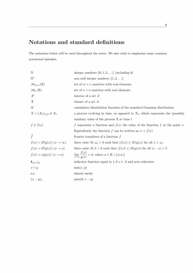
Notations and standard definitions
The notations below will be used throughout the notes. We also wish to emphasize some common
notational mistakes.
N integer numbers 0, 1, 2, . . . (including 0)
N∗ non null integer numbers 1, 2, . . .
Mm,n (R) set of m× n matrices with real elements
Mn (R) set of n× n matrices with real elements
Ao interior of a set A
A closure of a set A
N cumulative distribution function of the standard Gaussian distribution
X = (Xt)t≥0 = Xt a process evolving in time, as opposed to Xt, which represents the (possibly
random) value of the process X at time t
f = f(x) f represents a function and f(x) the value of the function f at the point x.
Equivalently the function f can be written as x 7→ f(x)
f Fourier transform of a function f
f(x) = O(g(x)) (x→ ∞) there exist M,x0 > 0 such that |f(x)| ≤M |g(x)| for all x > x0
f(x) = O(g(x)) (x→ a) there exist M, δ > 0 such that |f(x)| ≤M |g(x)| for all |x− a| < δ
f(x) = o(g(x)) (x→ a) limx→a
f(x)
g(x)= 0, where a ∈ R ∪ ±∞
11x∈A indicator function equal to 1 if x ∈ A and zero otherwise
x ∧ y min(x, y)
a.s. almost surely
(x− y)+ max(0, x− y)
Chapter 1
Descriptive Statistics and Python
1.1 Python for Statistics
1.1.1 A quick introduction to programming languages
Computing and programming are ubiquitous, in every area of every-day life, and are becoming
increasingly important to deal with large flows of information. On financial markets, programming
is fundamental to analyse time series of data, to evaluate financial derivatives, to run risk analyses,
and to trade at high frequency, for example. Which programming language to use depends on
one’s needs, and the main factor is time: there are two types of times one should consider:
• Execution time is the time it takes to run the programme itself;
• Development time is the time it takes to write the code.
For ultra high-frequency trading, for instance, execution time is the most important, as the algo-
rithm needs to make a decision very quickly. For long-term trading strategies, however, execution
time is less important, and one might favour quicker development time.
1.1.2 Statically typed languages
For short execution time, lower level languages, which compile directly to machine code, are pre-
ferred. The often use static typing, namely data types have to be specified. C++ is the main
example, and has been the main language used in quantitative finance; however, there is a non-
negligible entry cost to it, understanding its underlying concepts such as memory allocation or
pointers. Java is also a statically typed language, but automatically manages low-level memory
allocation; that said, it does not compile directly to machine code, and needs a Java Virtual Ma-
chine to execute the Java bytecode generated by the programme. Historically slower than C++
(because of the virtual machine layer), recent advances have now made their speeds comparable.
7

1.2. Python 8
1.1.3 Interpreted languages
When execution time is not the priority, and development time is preferred (for example for long-
term strategies), one can instead use interpreted languages, such as Matlab, Python, or R. While
the execution time is slower, these languages are dynamically typed, so that variables’ types are
automatically recognised by the programme and do not need to be specified by the user. Matlab
has been a popular language in quantitative finance, and is still around because of its legacy code.
However, in recent years, R (historically the preferred language for Statistics) and Python have
been taking over, as they are open source and the range of available packages for applications
has been growing exponentially. They are obviously slower than lower level languages, and some
in-between languages have recently appeared, in particular Julia, which, when first run, generates
machine code for execution.
1.1.4 Functional and query languages
1.2 Python
1.2.1 Python in Finance
A large number of financial companies, banks, hedge funds, asset managers,... have recently
adopted Python. JP Morgan’s Quartz, based on Python, is used for pricing and risk analyses;
Bank of America has its own version called Athena. One major drawback of Python is its Global
Interpreter Lock (GIL), which only allows one thread to execute at every point in time, making it
difficult to parallelise code. Some Python libraries bypass the issue, for example the multiprocessing
one, allowing the user to use multiple cores. Cython, on the other hand, is a static compiler for
Python, and allows to convert some slow Python code (in particular loops) into much faster C
versions.
1.2.2 General Python libraries
Python 3.5 is the default version of Pythoninstead of 2.7. It is well supported by many packages
to analyse data and perform statistical analysis.
• NumPy is the fundamental basic package for scientific computing with Python.
• SciPy supplements NumPy.
• pandas is a high-performance library for data analysis.
• matplotlib is the standard Python library for plots and graphs.

1.3. Online data sources 9
1.2.3 Python for Economics and Finance
• quantdsl is a functional programming language for financial derivatives.
• statistics is a built-in Python library for basic statistical computations.
• ARCH: tools for econometrics.
• statsmodels allows to explore data, estimate statistical models, and perform statistical tests.
• QuantEcon: library for economic modelling
1.2.4 Python libraries for plotting
• matplotlib is the standard Python library for plots and graphs. It is fairly basic but can
basically, with enough commands, generate any graphs.
• Seaborn is a powerful plotting library built on top of matplotlib.
1.2.5 Python libraries for Machine learning
• scikit-learn adds to SciPy and NumPy common machine learning and data mining algo-
rithms, such as clustering, regression, and classification.
• Theano has machine learning algorithms using the computer’s GPU, and is hence extremely
powerful for deep learning and heavy tasks.
• TensorFlow is Google-supported machine learning library based on a multi-layer architec-
ture.
1.3 Online data sources
Python makes it straightforward to query online databases directly, without having to import data
locally.
Economics database
An important database for economists is FRED, a vast collection of time series data maintained by
the St. Louis Federal Reserve. For example, the entire series for the US civilian unemployment rate
is available at https://research.stlouisfed.org/fred2/series/unrate/downloaddata/UNRATE.csv.
Another useful data for Economics data is the World Bank, which collects and organises data
on a huge range of indicators.

1.3. Online data sources 10
Finance database
Yahoo Finance, Google Finance are publicly available. Options market data, though, are not, but
can be accessed via WRDS/OptionMetrics.
Other interesting databases
• Google Trends Can you give some reasons explaining this graph and that one?
• Google Books
• Million Song Dataset
• Comprehensive list of available data
Chapter 2
Applied Multivariate Statistical
Analysis
2.1 A short introduction to Matrix algebra
In this part, we recall some fundamental definitions, tools and properties of finite-dimensional alge-
bra. Unless otherwise specified–chiefly because of the financial applications in mind–all quantities
will be real valued.
2.1.1 Introductory tools
For m,n integers, we shall denote by Mm,n the space of matrices with real entries with m rows
and n columns, endowed with the scalar product
⟨A,B⟩ :=m∑i=1
n∑j=1
aijbij , for any A,B ∈ Mm,n,
and the associated Euclidean norm ∥A∥ := ⟨A,A⟩1/2, where we use capital letters to denote
matrices, and lower-case letters for its entries, such as A = (ai,j)1≤i≤m,1≤j≤n, and we denote
by A⊤ the transpose of the matrix A, i.e. A⊤ = (aj,i)1≤j≤n,1≤i≤m ∈ Mn,m. For A ∈ Mm,n and
B ∈ Mn,p, the product C := AB belongs to Mm,p and ci,k =∑n
k=1 aijbjk. Whenever m = n, the
space of square matrices (and corresponding indices) will be denoted by Mn for simplicity. The
matrix In is the identity matrix in Mn, and Om,n the null matrix in Mm,n.
Definition 2.1.1. Let A ∈ Mn.
• The matrix A is called orthogonal if AA⊤ = A⊤A = In;
• The rank of A, denoted rank(A) is the maximum number of linearly independent rows;
11
2.1. A short introduction to Matrix algebra 12
• Trace: Tr(A) :=∑n
i=1 aii;
• Determinant:
det(A) :=∑
(−1)|τ |a1,τ1 · · · an,τn ,
over all permutations τ ∈ 1, · · · , n, and |τ | = 0 if the permutation is a product of an even
number of transpositions, and |τ | = 1 otherwise;
• if det(A) = 0 then the inverse matrix A−1 exists and AA−1 = A−1A = In;
Exercise 1. Following the notations in Definition 2.1.1, let α ∈ R, prove the following identities:
(a) det(αA) = αn det(A);
(b) det(AB) = det(BA) = det(A) det(B);
(c) Tr(AB) = Tr(BA);
(d) ⟨A,B⟩ = Tr(A⊤B) = Tr(AB⊤);
(e) 0 ≤ rank(A) ≤ m ∧ n;
(f) rank(A) = rank(A⊤) = rank(AA⊤);
(g) if A ∈ Mn and det(A) = 0,, then det(A)−1 = det(A−1);
(h) if A is orthogonal, then | det(A)| = 1;
2.1.2 Spectral Theory for matrices
In this section, we consider a square real-valued matrix A ∈ Mn. The spectral theory for matrices
is based on the following definition:
Definition 2.1.2. The characteristic polynomial PA of the matrix A is defined as
PA(λ) := det(A− λI).
It is easy to see that deg(PA) = n, and its n (possibly complex) roots are called the eigenvalues
of A. A root with algebraic multiplicity equal to one is called a simple eigenvalue, and we usually
denote the set of eigenvalues σ(A). For any λ ∈ σ(A), a non-null vector u ∈ Rn satisfying Au = λu
is called the associated eigenvector. We shall further denote by ρ(A) := max|λ| : λ ∈ σ(A) the
spectral radius of A.
Exercise 2.
• Show that the eigenvalues of a square symmetric matrix are real.
• Let P be a polynomial. Show that, for any λ ∈ σ(A), then P (λ) ∈ σ(P (A)).
2.1. A short introduction to Matrix algebra 13
• Show that PA(A) = 0.
• Show that det(A) =∏
λ∈σ(A)
λ, and that Tr(A) =∑
λ∈σ(A)
λ;
Theorem 2.1.3 (Jordan (spectral) decomposition). Any symmetric matrix A ∈ Mn admits a
decomposition of the form A = ΓΛΓ⊤, where Λ is the diagonal matrix of all eigenvalues of A,
and Γ the orthogonal matrix consisting of the eigenvectors of A.
Since the matrix Λ is diagonal, we shall use the standard notation Λ = Diag(λ1, . . . , λn).
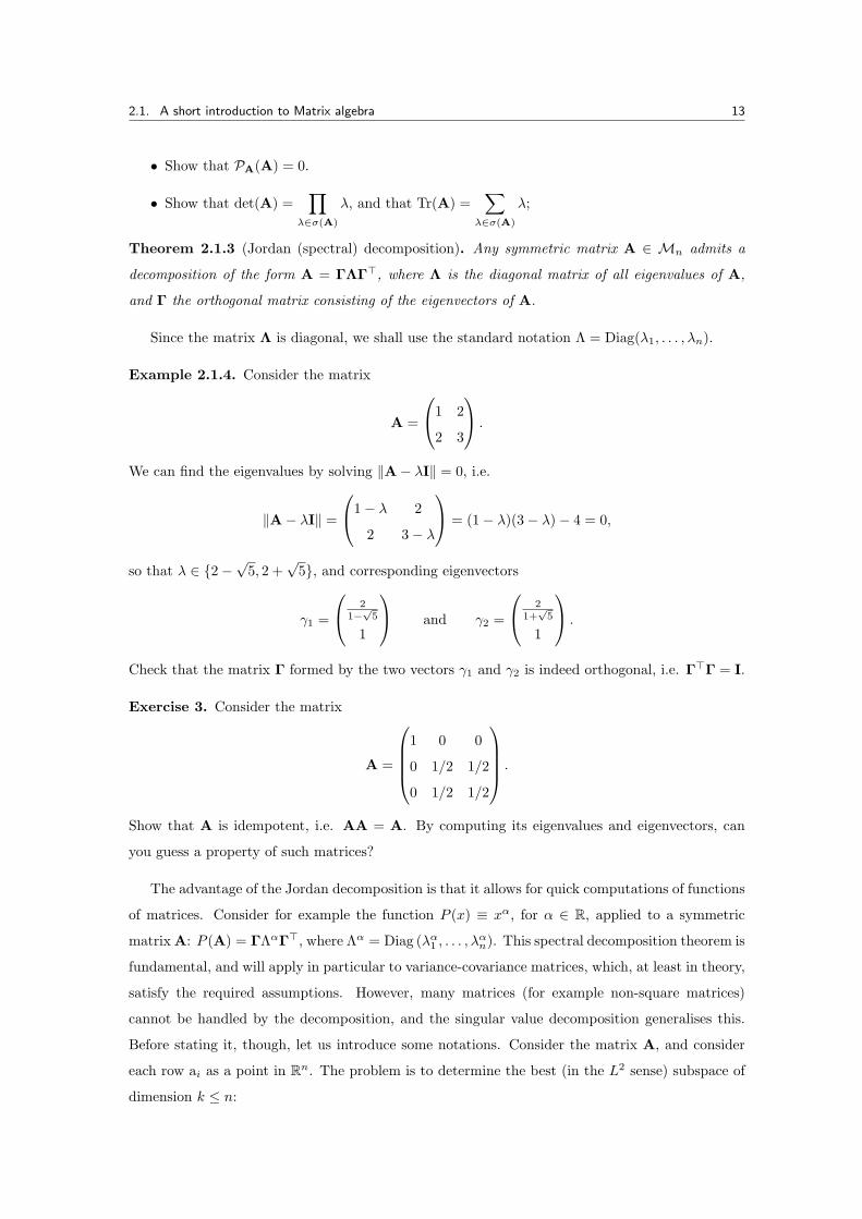
Example 2.1.4. Consider the matrix
A =
1 2
2 3
.
We can find the eigenvalues by solving ∥A− λI∥ = 0, i.e.
∥A− λI∥ =
1− λ 2
2 3− λ
= (1− λ)(3− λ)− 4 = 0,
so that λ ∈ 2−√5, 2 +
√5, and corresponding eigenvectors
γ1 =
21−
√5
1
and γ2 =
21+
√5
1
.
Check that the matrix Γ formed by the two vectors γ1 and γ2 is indeed orthogonal, i.e. Γ⊤Γ = I.
Exercise 3. Consider the matrix
A =
1 0 0
0 1/2 1/2
0 1/2 1/2
.
Show that A is idempotent, i.e. AA = A. By computing its eigenvalues and eigenvectors, can
you guess a property of such matrices?
The advantage of the Jordan decomposition is that it allows for quick computations of functions
of matrices. Consider for example the function P (x) ≡ xα, for α ∈ R, applied to a symmetric
matrixA: P (A) = ΓΛαΓ⊤, where Λα = Diag (λα1 , . . . , λαn). This spectral decomposition theorem is
fundamental, and will apply in particular to variance-covariance matrices, which, at least in theory,
satisfy the required assumptions. However, many matrices (for example non-square matrices)
cannot be handled by the decomposition, and the singular value decomposition generalises this.
Before stating it, though, let us introduce some notations. Consider the matrix A, and consider
each row ai as a point in Rn. The problem is to determine the best (in the L2 sense) subspace of
dimension k ≤ n:
2.1. A short introduction to Matrix algebra 14
Definition 2.1.5. Let A := (a1, . . . , am) be a set of points in Rn. The best approximating k-
dimensional linear subspace of A is the linear subspace V ∈ Rk such that the distance from A
to V is minimised.
Consider the case k = 1; we are looking for a line through the origin, closest to the cloud of
points. By Pythagoras theorem, minimising the (square of the) distance of the cloud onto the
line is equivalent to maximising the squared length of the projection onto the line. Let v be a
unit vector along this line, and consider the projection of the point ai onto v. The projection
corresponds exactly to the vector ⟨ai, v⟩v, where the angle bracket here is nothing else than the
dot product a⊤i v. Since v is a unit vector, the length of this projection is equal to a⊤i v. Therefore,
by Pythagoras theorem, the distance from ai to V is equal to
Dist(ai,V)2 = a⊤i ai −(a⊤i v
)2,
and the distance between A and V is thus
Dist(A,V)2 =
m∑i=1
(a⊤i ai −
(a⊤i v
)2)= ∥A∥2F − ∥Av∥2, (2.1.1)
where ∥ · ∥F denotes the Frobenius norm ∥A∥2F := Tr(A⊤A). Since the first term is constant,
minimising this distance is equivalent to maximising ∥Av∥. The first singular vector v1 is the best
line fit (through the origin), defined as
v1 := argmax∥v∥=1
∥Av∥, (2.1.2)
and we call σ1(A) := ∥Av1∥ the first singular value. Note that, since (2.1.1) has to be non-
negative, the maximum value for σ1(A) is the Frobenius norm of A, which corresponds to all the
points a1, . . . , am lying on the same line. We can then iterate this procedure to define the second
singular vector and value as
v2 := argmaxv⊥v1,∥v∥=1
∥Av∥ and σ2(A) := ∥Av2∥.
Clearly, the sequence of singular values is decreasing, and hence two cases can occur: either we
reach n iterations, and there is hence no more vector v to choose, or we reach a level r such
that σr+1(A) = 0. In the latter case, this means that the data A lies fully in a r-dimensional
subspace, spanned by the basis v1, . . . , vr. The following result–stated without proof (not too
hard, though)–justifies this algorithm:
Proposition 2.1.6 (Greedy Algorithm). Let A ∈ Mm,n and v1, . . . , vr its singular vectors con-
structed as above. For any 1 ≤ k ≤ r, the subspace spanned by v1, . . . , vk is the best fit of dimen-
sion k for the matrix A.
2.1. A short introduction to Matrix algebra 15
Fix a row i. Since the vectors v1, . . . , vr span the space of all rows of the matrix A, then clearly
a⊤i v = 0 for all v orthogonal to these vectors. Therefore, we can write∑r
j=1
(a⊤i vj
)2= ∥ai∥2
since vi is a unit vector orthogonal to (v1, . . . , vi−1, vi+1, . . . , vr), and hence
n∑i=1
∥ai∥2 =n∑
i=1
r∑j=1
(a⊤i vj
)2=
r∑j=1
n∑i=1
(a⊤i vj
)2=
r∑j=1
∥Avj∥2 =r∑
j=1
σ2j (A),
which in fact defines the so-called Frobenius norm.
Definition 2.1.7. The sequence of vectors (ui)i=1,...,n defined by ui :=Aviσi(A)
are called the left
singular vectors of A, and the vi are the right singular vectors.
Theorem 2.1.8. Both left and right singular vectors are orthogonal.
The fact that the right singular vectors are orthogonal is trivial from their definition. We can
prove by induction that so are the left singular vectors, but we shall omit the proof for sake of
brevity here.
Theorem 2.1.9 (Singular Value decomposition). Any matrix A ∈ Mm,n with rank r admits a
decomposition of the form A = UΛ1/2V⊤, where Λ = Diag (σ1(A), . . . , σr(A)), and U ∈ Mm,r
and V ∈ Mn,r the matrices composed of the left and right singular vectors of A.
Proof. We want to show that the first r singular vectors form a linear subspace maximising the
sum of squared projections of A onto it. It is trivial if r = 1, since the singular vector v1 is the
solution of the maximisation problem (2.1.2). Let now W, with orthonormal basis (w1,w2) be
any best approximating two-dimensional linear subspace for A. We are interested in maximising
the quantity ∥Aw1∥2 + ∥Aw2∥2, and we pick the vector w2 ⊥ v1. Indeed, either v1 is already
orthogonal toW (trivial case), or it is not, and we letw1 be the orthogonal projection of v1 ontoW,
and take w2 as a unit vector orthogonal to w1. By construction, the vector v1 maximises ∥Av∥,
so that ∥Av1∥ ≥ ∥Aw1∥, and ∥Av2∥ ≥ ∥Aw2∥ because w2 ⊥ v1. Therefore ∥Av1∥2 + ∥Av2∥2 ≥
∥Aw1∥2 + ∥Aw2∥2 as desired. The general r-dimensional case can be deduced by induction.
The most useful application of Singular Value Decomposition in this course will be PCA, which
we will see in full details later. It also has many applications, in particular to compute the so-called
pseudo-inverse, and for image compression. To convince yourself, at least intuitively, consider the
transmission of an image, where the matrixA ∈ Mn,n represents the pixel description of the image.
For large n, the transmission cost is of order n2. Suppose that, instead of transmitting A, we only
transmit the first k singular values and left and right singular vectors; this would cost O(kn)
operations. Of course, details are lost, and quality decreases, but, by picking the dimension k, one
effectively chooses the size of the resolution. This can be formalised, and is, in fact, the content of
the following theorem, which forms the basis of image reduction:
2.1. A short introduction to Matrix algebra 16
Theorem 2.1.10 (Eckart-Young-Mirsky Theorem). Let A ∈ Mm,n with rank r, and fix some
k ≤ r. The solution to the optimisation problem
minA
∥∥∥A− A∥∥∥F: rank(A) ≤ k
is given by A = U1Λ
1/21 V⊤
1 . Here, starting from the SVD of A = UΛ1/2V⊤, we write
U =(U1 U2
), Λ =
Λ1 Ok,r−k
Or−k,k Λ2
, V =(V1 V2
),
with U1 ∈ Mm,k, V1 ∈ Mn,k, Λ1 ∈ Mk,k
IPython notebook SVD.ipynb
IPython notebook SVD ImageCompression.ipynb
2.1.3 Quadratic forms
Let A be a square matrix in Mn. We call QA(x) := x⊤Ax the quadratic form, from Rn to R,
associated to A.
Definition 2.1.11. The matrix A is said to be positive semi-definite (resp. positive definite), and
we write A ≥ On (resp. A > On), if QA(x) ≥ 0 (resp. QA(x) > 0) for all non-zero vector x ∈ Rn.
We shall denote by M+n (resp. M++
n ) the space of symmetric positive semi-definite (resp.
positive definite) matrices in Mn.
Example 2.1.12. The identity matrix In is positive definite.
Theorem 2.1.13. If A is symmetric, then QA(x) = y⊤Λy for any x ∈ Rn, with y := Γ⊤x,
where Λ and Γ arise from the Jordan decomposition of A.
Proof. Since A = ΓΛΓ⊤ from Theorem 2.1.3, then x⊤Ax = x⊤ΓΛΓ⊤x = y⊤Λy, with y = Γ⊤x,
and the theorem follows.
Proposition 2.1.14. Let A ∈ M+n . For any N ∈ N, there exists a unique B ∈ M+
n such that A = BN .
Quadratic forms provide an easy way to check positivity of eigenvalues:
Proposition 2.1.15. The matrix A is positive definite if and only if minλ∈σ(A) λ > 0.
Proof. Since A > On, then 0 < QA(x) = y⊤Λy by Theorem 2.1.13, and the proposition follows.
Corollary 2.1.16. If A is positive definite, then A−1 exists and ∥A∥ > 0.
2.1. A short introduction to Matrix algebra 17
Exercise 4. Compute the quadratic forms of the identity matrix in Mn and of the matrices 1 −1
−1 1
and
1 0
0 −1
,
and determine their (absence of?) positivity.
Positive matrices appear very often in mathematical finance and in Statistics (in particular as
covariance matrices), and admit a certain number of useful factorisations. Recall that a matrix T
is called upper triangular if tij = 0 whenever i > j.
Proposition 2.1.17. If A > On (resp. A ≥ On) then there exists a unique (resp. non-unique)
upper triangular matrix T ∈ Mn with strictly positive (resp. non-negative) diagonal elements such
that A = T⊤T.
This apparently simple proposition allows, for example, to simulate general Gaussian processes
simply from the knowledge of their covariance matrices. The following theorem will be funda-
mental when analysing reduction of variance in multivariate statistics, in particular for Principal
Component Analysis:
Theorem 2.1.18. Let A and B two symmetric matrices in Mn with B > On. Then
minx:QB(x)=1
QA(x) = minσ(B−1A) ≤ maxσ(B−1A) = maxx:QB(x)=1
QA(x).
Proof. Using the Jordan Decomposition, and writing the corresponding matrix as an index, we
can write B1/2 = ΓBΛ1/2B Γ⊤
B. Setting y := B1/2x, we can therefore write
maxx:QB(x)=1
QA(x) = maxy:|y∥=1
QA(B−1/2y).
Using the Jordan Decomposition again, we can write (B−1/2)⊤AB−1/2 = ΓΛΓ⊤, so that, with
z := Γ⊤y, we have ∥z∥ = ∥Γ⊤y∥ = ∥y∥ since Γ is orthogonal, and hence
maxy:|y∥=1
QA(B−1/2y) = maxz:∥z∥=1
z⊤Λz = maxz:∥z∥=1
n∑i=1
λiz2i ≤
(max
λ∈σ(A)λ
)(max
z:∥z∥=1∥z∥)
= maxσ(A).
Clearly the maximum is attained at the point z = (1, 0, . . . , 0)⊤. Since the matrices B−1A and
B−1/2AB−1/2 have the same eigenvalues, the theorem follows.
2.1.4 Derivatives
Let x ∈ Rn and y ∈ Rm related by y = ψ(x), where ψ : Rn → Rm is a smooth function. The
Jacobian of the transformation is defined as
∇Xψ(x) =(∂xjyi
)1≤i≤m,1≤j≤n
∈ Mm,n.
Example 2.1.19. Show that the following derivatives hold:
2.2. Essentials of probability theory 18
• ∇x (Ax) = A, for any A ∈ Mm,n;
• ∇x
(x⊤A
)= A⊤, for any A ∈ Mn,m;
• ∇X (QA(x)) = x⊤(A+A⊤), for any A ∈ Mn;
• ∇2X (QA(x)) =
(A+A⊤), for any A ∈ Mn.
2.1.5 Block matrices
For large matrices, it is sometimes convenient to decompose them into blocks of sub-matrices.
Think for example of the covariance matrix of the S&P constituents, where one may be interested
in sub-portfolios only. Let A ∈ Mn be a square matrix with n = p+ q (p, q ≥ 1), partitioned as
A =
A11 A12
A21 A22
,
where A11 ∈ Mp, A22 ∈ Mq, A12 ∈ Mp,qq and A21 ∈ Mq,p. Whenever it exists, the inverse
matrix is denoted by
A−1 =
A11 A12
A21 A22
,
and the blocks of the inverse are related to the original blocks through the following result, the
proof of which is left as a simple yet tedious exercise:
Proposition 2.1.20. Assuming all terms exist, the following identities hold:
A11 =(A11 −A12A
−122 A21
)−1, A12 = −A11A12A
−122 ,
A22 =(A22 −A21A
−111 A12
)−1, A21 = −A22A21A
−111 .
Proposition 2.1.21. The following hold:
det
A11 Op,q
A21 A22
= det(A11) det(A22) = det
A11 A21
Oq,p A22
and, assuming they exist.
det(A) = det(A11) det(A22 −A21A
−111 A12
)= det(A22) det
(A11 −A12A
−122 A21
).
2.2 Essentials of probability theory
We provide here a brief overview of standard results in probability theory and convergence of
random variables needed in these lecture notes.
2.2. Essentials of probability theory 19
2.2.1 PDF, CDF and characteristic functions
In the following, (Ω,F ,P) shall denote a probability space and X a random variable defined on it.
We define the cumulative distribution function F : R → [0, 1] of X by
F (x) := P (X ≤ x) , for all x ∈ R.
The function F is increasing and right-continuous and satisfies the identities limx↓−∞
F (x) = 0 and
limx↑∞
F (x) = 1. If the function F is absolutely continuous, then the random variable X has a
probability density function f : R → R+ defined by f(x) = F ′(x), for all real number x. Note that
this in particular implies the equality F (x) =∫ x
−∞ f(u)du. Recall that a function F : D ⊂ R → R
is said to be absolutely continuous if for any ε > 0, there exists δ > 0 such that the implication∑n
|bn − an| < δ =⇒∑n
|F (bn)− F (an)| < ε
holds for any sequence of pairwise disjoint intervals (an, bn) ⊂ D. Define now the characteristic
function ϕ : R → C of the random variable X by
ϕ(u) := E(eiuX
).
Note that it is well defined for all real number u and the identity |ϕ(u)| ≤ 1 always holds on R. Its
extension to the complex plane (u ∈ C) is more subtle; while it is fundamental for option pricing,
it is less so for Statistics, and we shall leave it aside in these notes.
2.2.2 Some useful inequalities
We recall here a few inequalities that appear frequently in Probability and Statistics. We shall
always consider random variables supported on the whole real line. The results below are not
restricted to this case, though, but notations are simpler then.
Proposition 2.2.1 (Markov Inequality). Let f be an increasing function and X a random variable
such that E[f(X)] is finite. Then, for any x ∈ R such that f(x) > 0,
P(X ≥ x) ≤ E[f(X)]
f(x).
Proof. Since f is increasing, then
P(X ≥ x) ≤ P(f(X) ≥ f(x)) = E(11f(X)≥f(x)
)≤ E
(f(X)
f(x)11f(X)≥f(x)
)≤ E (f(X))
f(x).
The following proposition is in fact an immediate corollary and is left as a simple exercise.
Proposition 2.2.2 (Chebychev Inequality). If X ∈ L2(R), then, for any x > 0,
P(|X| ≥ x) ≤ E(X2)
x2and P(|X − E(X)| ≥ x) ≤ V(X2)
x2.
2.2. Essentials of probability theory 20
Proposition 2.2.3 (Holder Inequality). Let p ∈ (1,∞) and q such that p−1 + q−1 = 1. If X
and Y are random variables such that E(|X|p) and E(|Y |q) are finite, then E(|XY |) is finite and
E(|XY |) ≤ E (|X|p)1/p E (|Y |q)1/q .
Proof. Since the logarithm function is convex, the identity
log(x)
p+
log(y)
q≤ log
(x
p+y
q
)holds for all x, y > 0. Taking exponential on both sides, this is obviously equivalent to x1/py1/q ≤xp + y
q . Setting x = |X|p/E(|X|p) and y = |Y |q/E(|Y |p) yields the result directly.
The following inequality is a simple corollary, the proof of which is left as an exercise.
Proposition 2.2.4 (Lyapunov Inequality). Let 0 < p < q, and X a random variable such that
E(|X|q) is finite. Then
E(|X|p)1/p ≤ E(|X|q)1/q.
The kurtosis of a distribution X is defined as
κ :=E[(X − E(X))
4]
V(X)2,
and the excess kurtosis κ+ := κ− 3.
Exercise 5. Using Lyapunov’s Inequality, show that the excess kurtosis is always greater than −2.
Show that this lower bound is attained for the Bernoulli distribution with equal chances.
Kurtosis measures the fatness of a distribution tails. Distributions can be classified as follows:
• Mesokurtic (κ+ = 0): the Gaussian distribution for example;
• Leptokurtic (κ+ > 0) distributions correspond to fat tails, and are of fundamental impor-
tance to describe returns of financial assets (in particular on Equity markets). The Student,
Poisson, Laplace or Exponential distributions all belong to this category;
• Platykurtic (κ+ < 0) correspond to thin-tail distributions, such as the uniform distribution.
Note that the Lyapunov Inequality in particular implies the sequence of inequalities for the mo-
ments of X,
E(|X|) ≤ E(|X|2)1/2 ≤ · · · ≤ E(|X|q)1/q,
as long as the last one is finite for some integer q. This can be generalised as follows, the proof of
which is left as an exercise:
Proposition 2.2.5 (Jensen Inequality). Let f be a convex function and X a random variable such
that E[f(X)] is finite. Then f(E(X)) ≤ E[f(X)].
2.2. Essentials of probability theory 21
Proposition 2.2.6 (Cauchy-Schwarz Inequality). Let X and Y be two square-integrable random
variables with E|XY | finite. Then (E(XY ))2 ≤ (E|XY |)2 ≤ E(X2)E(Y 2). The inequalities are
equalities if X is almost surely a linear transformation of Y .
Theorem 2.2.7 (Hoeffding Inequality). Let X1, . . . , Xn be centered iid random variables with
ai ≤ Xi ≤ bi. For any ε > 0, and any z > 0,
P
(n∑
i=1
Xi ≥ ε
)≤ e−zε
n∏i=1
exp
(z2(bi − ai)
2
8
).
Exercise 6. Let X1, . . . , Xn be a sequence of iid Bernoulli(p) random variables. Using Theo-
rem 2.2.7, show that
P
(∣∣∣∣∣ 1nn∑
i=1
Xi − p
∣∣∣∣∣ > ε
)≤ 2e−2nε2 , for any ε > 0.
2.2.3 Gaussian distribution
A random variable X is said to have a Gaussian distribution (or Normal distribution) with mean
µ ∈ R and variance σ2 > 0, and we write X ∼ N(µ, σ2
)if and only if its density reads
f(x) =1
σ√2π
exp
(−1
2(x− µ)
2
), for all x ∈ R.
For such a random variable, the following identities are obvious:
E(eiuX
)= exp
(iµu− 1
2u2σ2
), and E
(euX
)= exp
(µu+
1
2u2σ2
),
for all u ∈ R. The first quantity is the characteristic function whereas the second one is the Laplace
transform or the random variable. If X ∈ N(µ, σ2
), then the random variable Y := exp(X) is
said to be lognormal and
E(Y ) = exp
(µ+
1
2σ2
)and E
(Y 2)= exp
(2µ+ 2σ2
).
2.2.4 Convergence of random variables
We recall here the different types of convergence for family of random variables (Xn)n≥1 defined
on a probability space (Ω,F ,P). We shall denote Fn : R → [0, 1] the corresponding cumulative
distribution functions and fn : R → R+ their densities whenever they exist. We start with a
definition of convergence for functions, which we shall use repeatedly.
Definition 2.2.8. The family (hn)n≥1 of functions from R to R converge pointwise to a function
h : R → R if and only if the equality limn↑∞
hn(x) = h(x) holds for all real number x.
This is a notoriously weak form of convergence, which, in particular does not preserve continuity
(check for example the sequence hn(x) = xn on [0, 1]). It will however suffice here.
2.2. Essentials of probability theory 22
Convergence in distribution
This is the weakest form of convergence, and is the one appearing in the Central Limit Theorem.
Definition 2.2.9. The family (Xn)n≥1 converges in distribution—or weakly or in law—to a ran-
dom variable X if and only if (Fn)n≥1 converges pointwise to a function F : R → [0, 1], i.e. if
limn↑∞
Fn(x) = F (x),
holds for all real number x where F is continuous. Furthermore, F is the CDF of X.
Example 2.2.10. Consider the family (Xn)n≥1 such that each Xn is uniformly distributed on
the interval[0, n−1
]. We then have Fn(x) = nx11x∈[0,1/n] + 11x≥1/n. It is clear that the family
of random variable converges weakly to the degenerate random variable X = 0. However, for any
n ≥ 1, we have Fn(0) = 0 and F (0) = 1.
Example 2.2.11. Weak convergence does not imply convergence of the densities, even when they
exist. Consider the family such that fn(x) =(1− cos (2πnx)
)11x∈(0,1).
Even though convergence in law is a weak form of convergence, it has a number of fundamental
consequences for applications. We list them here without proof and refer the interested reader
to [6] for details
Corollary 2.2.12. Assume that the family (Xn)n≥1 converges weakly to the random variable X.
Then the following statements hold
1. limn↑∞ E (h(Xn)) = E (h(X)) for all bounded and continuous function h.
2. limn↑∞ E (h(Xn)) = E (h(X)) for all Lipschitz function h.
3. limP (Xn ∈ A) = P (X ∈ A) for all continuity sets A of X.
4. (Continuous mapping theorem). The sequence (h(Xn))n≥1 converges weakly to h(X) for
every continuous function h.
The following theorem shall be of fundamental importance in many applications, and we there-
fore state it separately.
Theorem 2.2.13 (Levy’s continuity theorem). The family (Xn)n≥1 converges weakly to the ran-
dom variable X if and only if the sequence of characteristic functions (ϕn)n≥1 converges pointwise
to the characteristic function ϕ of X and ϕ is continuous at the origin.
Exercise 7. Consider the sequence (Xn)n≥0, where Xn ∼ N (µn, σ2n), and assume that limn↑∞ µn
and limn↑∞ σ2n exist. What can you conclude about the weak limit of the sequence (Xn)n≥0?
2.2. Essentials of probability theory 23
Convergence in probability
Definition 2.2.14. The family (Xn)n≥1 converges in probability to X if, for all ε > 0, we have
limn↑∞
P (|Xn −X| ≥ ε) = 0.
Remark 2.2.15. The continuous mapping theorem still holds under this form of convergence.
Almost sure convergence
This form of convergence is the strongest form of convergence and can be seen as an analogue for
random variables of the pointwise convergence for functions.
Definition 2.2.16. The family (Xn)n≥1 converges almost surely to the random variable X if
P(limn↑∞
Xn = X
)= 1.
Convergence in mean
Definition 2.2.17. Let r ∈ N∗. The family (Xn)n≥1 converges in the Lr norm to the random
variable X if the r-th absolute moments of Xn and X exist for all n ≥ 1 and if
limn↑∞
E (|Xn −X|r) = 0.
The following theorem makes the link between the different modes of convergence.
Theorem 2.2.18. The following statements hold:
• Almost sure convergence implies convergence in probability.
• Convergence in probability implies weak convergence.
• Convergence in the Lr norm implies convergence in probability.
• For any r ≥ s ≥ 1, convergence in the Lr norm implies convergence in the Ls norm.
2.2.5 Laws of large numbers and Central Limit Theorem
Consider an iid sequence (X1, . . . , Xn) of random variables, with common finite mean µ and com-
mon variance σ2, and define the arithmetic mean Xn := n−1∑n
i=1Xi. Direct computation yields
E(Xn) = µ and V(Xn) = σ2/n. The law of large numbers, presented below, is one of the funda-
mental results in probability, and is a key ingredient to prove convergence and bias of statistical
estimators.
Theorem 2.2.19. The weak law of large numbers state that the random variable Xn converges in
probability to µ as n tends to infinity. The strong law of large numbers ensures that the convergence
in fact holds almost surely.

2.3. Introduction to statistical tools 24
Note that, for the law of large numbers, weak or strong, to hold, we only require finiteness of
the first moment, not of the second moment, although the proof when the latter is not finite is
more involved. When the second moment is finite, we have the more precise formulation:
Theorem 2.2.20 (Central Limit Theorem). If both µ and σ are finite, then the sequence (Xn −
µ)/(σ/√n) converges in distribution to a centered Gaussian distribution with unit variance, or else
limn↑∞
P(Xn − µ
σ/√n
≤ x
)= FN (0,1)(x), for all x ∈ R.
2.3 Introduction to statistical tools
In this section, we shall let X = (X1, . . . , Xn) denote a vector of size n (or equivalently X ∈ Mn,1)
with random entries.
2.3.1 Joint distributions and change of variables
Let X denote a random vector taking values in Rn. Its joint density distribution (whenever it
exists) is the function f : Rn → R+ such that
FX(x) := P(X ≤ x) =
∫ x1
−∞· · ·∫ xn
−∞f(y1, . . . , yn)dy1 · · · dyn, for any x ∈ Rn.
For any i = 1, . . . , n, the marginal distribution of Xi is then given by
FXi(x) = lim(x1,...,xi−1,xi+1,...,xn)↑∞
FX(x).
In the continuous case, we shall always assume that F admits a non-negative density with respect
to the Lebesgue measure on Rn, so that
fX(x) = ∇xFX(x)
is well defined for all x ∈ Rn and satisfies∫Rn fX(x)dx = 1. For each i ∈ 1, . . . , n, the marginal
density function fi : R → R+ is defined as
fi(xi) :=
∫Rn−1
f(y1, . . . , yi−1, xi, yi+1, . . . , yn)dy1 · · ·dyi−1dyi+1 · · ·dyn.
We shall say that the random components of X are independent if
fX(x) =
n∏i=1
fi(xi), for any x ∈ Rn.
In the discrete case, the random vector X takes a finite number of values (x1, . . . , xm) for some
integer m, and the marginal law of Xi is therefore given by
P(Xi = xji ) =∑
k1,...,ki−1,ki+1,...,kn
P(X1 = xk1
1 , . . . , Xi−1 = xki−1
i−1 , Xi = xji , Xi+1 = xki+1
i+1 , . . . , Xn = xknn
).
2.3. Introduction to statistical tools 25
Remark 2.3.1. The marginal laws do not fully determine the joint law. Consider for example
the following two functions:
f(x, y) :=1
2πexp
(−x
2 + y2
2
)and g(x, y) :=
1 + xy11[−1,1](x)11[−1,1](y)
2πexp
(−x
2 + y2
2
).
Show that they are both genuine two-dimensional density functions and that their marginals are
all Gaussian.
Let now X and Y be two random vectors in Rn and Rm respectively, admitting a joint marginal
density fX,Y. The conditional density of Y with respect to X is defined as
fY|X(y|x) :=
fY,X(y, x)
fX(x)if fX(x) = 0,
fY(y) if fX(x) = 0.
Assume now that X admits a differentiable probability distribution function with density fX, and
define Y := g(X) for some function g ∈ C1(Rn → Rn). Then Y admits a density function fY
given by
fY(y) = fX(g−1(y)
) ∣∣det (∇y(g−1(y)
)∣∣ ,where∇y(h(y)) = (∂yjhi(y))1≤i,j≤n is the Jacobian matrix, and where the inverse function theorem
gives ∂yg−1(y) = 1/∂xg(x).
Example 2.3.2. Given the random vector X ∈ Rn, which admits a smooth density, define Y :=
AX+ b, where A ∈ Mn is invertible, and b ∈ Rn. Then Y admits a density and
fX(x) =fY(A−1(x− b))
| det(A)|for all x ∈ Rn.
2.3.2 Mean, covariance and correlation matrices
Whenever it exists the moment of order p is defined as
E (Xp) :=
E(Xp
1 )...
E(Xpn)
∈ Rn.
The second moment, whenever it exists, will also play a fundamental role later, and is defined as
E(XX⊤) := (E(XiXj)
)1≤i,j≤n
∈ Mn.
Proposition 2.3.3. Whenever it exists, the matrix E(XX⊤) is symmetric positive semi-definite.
Proof. For any u ∈ Rn, we can write
u⊤E(XX⊤)u = E
(u⊤XX⊤u
)= E
(∥X⊤u∥2
)≥ 0.
Furthermore, E(XX⊤) > 0 unless there exists u ∈ Rn such that P(u⊤X = 0) = 1.
2.3. Introduction to statistical tools 26
Definition 2.3.4. For any X ∈ Rm and Y ∈ Rn, the matrix
Cov(X,Y) := E((X− E(X)) (Y − E(Y))
⊤)=(Cov(Xi, Yj)
)1≤i≤m,1≤j≤n
∈ Mm,n
is called the covariance matrix of X and Y. The variance-covariance matrix of X is defined as
V(X) := Cov(X,X). Furthermore, the correlation matrix between X and Y is defined as
Corr(X,Y) :=
(Cov(Xi, Yj)√V(Xi)V(Yj)
)1≤i≤m,1≤j≤n
∈ Mm,n.
The following properties are easy to prove and are left as an exercise:
Proposition 2.3.5. Let X ∈ Rm, Z ∈ Rm, Y ∈ Rn be random vectors. Show that
• Cov(X,X) = V(X);
• Cov(X,Y) = Cov(Y,X)⊤;
• Cov(X+ Z,Y) = Cov(X,Y) + Cov(Z,Y);
• V(X+ Z) = V(X) + V(Z) + Cov(X,Z) + Cov(Z,X);
• Cov(AX,BY) = ACov(X,Y)B⊤, for any A ∈ Mp,m, B ∈ Mq,n.
Two random vectors X ∈ Rm and Y ∈ Rn with finite second moments are said to be uncorre-
lated if Cov(X,Y) = Om,n. If the two vectors are independent, then
Cov(X,Y) = E((X− E(X)) (Y − E(Y))
⊤)= (E(X)− E(X)) (E(Y)− E(Y))
⊤= Om,n,
hence they are uncorrelated. The converse is not necessarily true, however, as can be seen in
Exercise 8 below. We finish this reminder on multivariate computations with the following simple
statement:
Lemma 2.3.6. If X ∈ Rn is a random vector with finite second moment, then, for any u ∈ Rn
and A ∈ Mm,n, we have the identities
E(u +AX) = u +AE(X) and V(u +AX) = AV(X)A⊤.
Exercise 8.
• Consider the one-dimensional case X ∼ N (0, 1) and Y := X2. Is the knowledge of the
covariance enough to conclude about independence here?
• Prove that the correlation coefficient always lies in [−1, 1];
• Prove the identity V(Y ) = V(E(Y |X)) + E(V(Y |X));
2.4. Multivariate distributions 27
2.3.3 Forecasting
The goal of this short section is not to have a full overview of forecasting, but only to show
how conditional expectations enter as optimal (in some sense) forecasting tools. For two square
integrable random vectors X ∈ Rm and Y ∈ Rn, we understand X as observed data, and we wish
to obtain some estimates for the unknown Y.
Definition 2.3.7. The random vector G(X), for some function G : Rm → Rn is called best
forecast if
E((Y −G(X))(Y −G(X))⊤
)≤ E
((Y −H(X))(Y −H(X))⊤
),
holds for any function H : Rm → Rn.
The following result is simple to prove, but provides a fundamental understanding of conditional
expectation as an optimal projection operator.
Theorem 2.3.8. If the joint law of X and Y admits a density, then G(X) = E(Y|X).
It will often happen, at least as first approximations, that the random variables under consid-
eration are Gaussian. We therefore need to be able to compute those conditional expectations and
variances.
Theorem 2.3.9. Let X ∼ Nn(µ,Σ) with µ ∈ Rn and Σ ∈ M+n,n, with the decomposition
X =
X1
X2
, µ =
µ1
µ2
, Σ =
Σ11 Σ12
Σ21 Σ22
,
where X1 ∼ Np(µ1,Σ11), X2 ∼ Nq(µ2,Σ22) and p + q = n. With Θ := Σ21Σ−111 , the random
variables X1 and X2 −ΘX1 are independent, and, almost surely,
E(X2|X1) = µ2 +Θ(X1 − µ1) and V(X2|X1) = Σ22 −ΘΣ12.
2.4 Multivariate distributions
2.4.1 A detailed example: the multinormal distribution
The Gaussian distribution is ubiquitous in Probability, Statistics and applications, and hence
deserve a dedicated treatment. We start with the easy one-dimensional case, stating and proving
a certain number of its properties, before delving into the multivariate case.
The univariate case
Definition 2.4.1. A real-valued random variable X is called standard Gaussian, and we write
X ∼ N (0, 1) if its probability distribution reads, for all x ∈ R,
P(X ∈ dx) =1√2π
exp
(−x
2
2
)dx.
2.4. Multivariate distributions 28
The following representation of its characteristic function is left as an exercise:
Proposition 2.4.2. The characteristic function of X ∼ N (0, 1) is given by
ϕX(z) := E(eizX
)= exp
(−z
2
2
), for all z ∈ R.
Proof. Since the density of X is known in closed form, we can write, for any z ∈ R,
ϕX(z) =1√2π
∫Rexp
iuz − u2
2
du = exp
(−z
2
2
)(1√2π
∫R−iz
exp
−u
2
2
du
).
Since the map z 7→ exp(−z2/2) is analytic on R, Cauchy’s theorem shows that(∫ r−iz
−r−iz
+
∫ r
r−iz
+
∫ −r
r
+
∫ −r−iz
−r
)exp
−z
2
2
dz = 0.
This identity allows us to write
1√2π
∫R−iz
exp
−u
2
2
du− 1 =
1√2π
[(∫R−iz
−∫R
)exp
−u
2
2
du
]= lim
r↑∞
(∫ r−iz
−r−iz
+
∫ −r
r
)1√2π
exp
−u
2
2
du
= limr↑∞
(∫ r−iz
r
+
∫ −r
−r−iz
)1√2π
exp
−u
2
2
du.
Since | exp(−z2/2)| = exp(−ℜ(z2)/2), then this limit is equal to zero, and the proposition follows.
Proposition 2.4.3. Let X ∼ N (0, 1). Then all moments exists,
E (Xp) =
0 if p is odd,
p!
2p/2(p/2)!if p is even,
and
E (|X|p) = 2p/2Γ((p+ 1)/2)
Γ(1/2), for all p ≥ 0.
Proof. Let p be even so that we can write p = 2n. Then
E(X2n) =1√2π
∫Rx2n exp
(−x
2
2
)dx =
√2
π
∫ ∞
0
x2n exp
(−x
2
2
)dx
=2n√π
∫Rzn−1/2e−zdz =
2n√πΓ
(n+
1
2
),
and the result follows from the fact that Γ(1/2) =√π and the recursion Γ(n + 1) = nΓ(n). The
proof for the absolute moments is similar and left as an exercise.
Gaussian random variables satisfy the following useful property:
Proposition 2.4.4. Let X ∼ N (µ,Σ) ∈ Rn be Gaussian random vector with independent compo-
nents. Then, for any u ∈ Rn, the sum S := u⊤X is also Gaussian with
E(S) = u⊤µ and V(S) = QΣ(u).
2.4. Multivariate distributions 29
The matrix case
We now extend the results from the univariate case above to the more interesting multi-dimensional
case. We denote by N (On, In) the Gaussian random vector Y = (Y1 . . . , Yn), where each Yi is
a univariate centered Gaussian random variable with unit variance. More generally, we define a
Gaussian vector as follows:
Definition 2.4.5. Let µ ∈ Rn and Σ ∈ M+n such that Σ = T⊤T (by Proposition 2.1.17). The
vector X is said to follow a Gaussian random distribution with mean µ and variance-covariance
matrix Σ, and we write X ∼ N (µ,Σ) if the equality X = µ+T⊤N (On, In) holds in distribution.
A simple way to understand this is to start from a random vector Z = (Z1, . . . , Zn), constituting
an iid sequence of standard Gaussian distributions. Its joint density then reads
fZ(z) =1
(2π)n/2exp
−∥z∥2
2
, for any z ∈ Rn.
Define now the random vector X := µ+T⊤Z, where µ ∈ Rn, and T ∈ Mn(R) a matrix of rank k.
If k < n, then Z is said to have a singular multivariate Gaussian distribution. If k = n, then T
has full rank and Σ := T⊤T is positive definite and X ∼ N (µ,Σ).
Proposition 2.4.6. Let X ∼ N (µ,Σ). Then E(X) = µ, V(X) = Σ, and
ϕX(u) := E(eiu
⊤X)= exp
iu⊤µ− 1
2u⊤Σu
, for all u ∈ Rn.
If furthermore Σ ∈ M++n , then X admits a density which reads
P(X ∈ dx) =dx
(2π)n/2 det(Σ)1/2exp
−1
2(x− µ)⊤Σ−1(x− µ)
, for all x ∈ Rn.
Exercise 9. Let X ∈ Mn. Prove the following properties:
• For any A ∈ Mm,n, u ∈ Rm, then AN (µ,Σ) + u∆=N (Aµ+ u,AΣA⊤);
• for any orthogonal matrix A ∈ Mn, AN (On, In)∆=N (On, In);
In the case of Gaussian random vectors, independence can be characterised simply through the
variance-covariance matrix:
Proposition 2.4.7. The components of X∆=N (µ,Σ) are independent if and only if Σ is diagonal.
Proof. The vectors X1, . . . , Xn are independent if and only if the equality
E(eiu
⊤X)=
n∏i=1
E(eiuiXi
)holds for all u ∈ Rn. We leave it to the reader to check this is indeed the case.

2.4. Multivariate distributions 30
2.4.2 Other useful distributions
Chi Square Distribution
Definition 2.4.8. Let X1, . . . , Xn for an iid sequence of centered Gaussian distributions with unit
variance. Then the law of Sn :=∑n
i=1X2i is called the χ2 distribution with n degrees of freedom,
and we write Sn ∼ χ2n.
It is easy to prove in particular that E(Sn) = n and V(Sn) = 2n, that it admits a density
fSn(x) =xn/2−1e−x/2
2n/2Γ(n/2), for all x ≥ 0,
where Γ(u) :=∫∞0zu−1e−zdz is the Gamma function, and its moment generating function reads
E(euSn
)= (1− 2u)
−n/2, for all u <
1
2.
Student Distribution
Definition 2.4.9. If Sn ∼ χ2n for some integer n and Z ∈ N (0, 1), then the ratio Tn := Z√
Sn/nis
called a Student distribution with n degrees of freedom, and we write Tn ∼ Tn.
One can show that its density reads
fTn(x) =Γ(n+12
)√nπΓ
(n2
) (1 + x2
n
)−(n+1)/2
, for all x ∈ R.
The expectation is finite if and only if n > 1, in which case E(Tn) = 0. Likewise, the variance is
finite if and only if n > 2, in which case V(Tn) = n/(n − 2). The moment generating function,
however, is always undefined.
Wishart distribution
We introduced above the χ2 distribution, as a sum of squared iid Gaussian distributions. Its
extension to the multivariate case is called the Wishart distribution, and will be fundamental in
the study of estimators for covariance matrices.
Definition 2.4.10 (Wishart Distribution). If X1, . . . ,Xn forms a sequence of Rp-valued inde-
pendent N (0,Σ) distributions, then the random matrix W :=∑n
i=1 XiX⊤i is called a Wishart
distribution, denoted by Wp(Σ, n).
We shall not dive into any details of this distribution here, but simply note that its density and
characteristic function are available in closed form.
2.5. Application: Markowitz and CAPM 31
2.5 Application: Markowitz and CAPM
We now show how to apply these tools from multivariate analysis in order to solve the so-called
Markowitz 1 efficient frontier problem. We consider n assets, and denote by X = (X1, . . . , Xn) the
vector of returns over a given period. Following earlier notations, the mean and covariance read
µ := (µ1, . . . , µn) = (E(Xi))i=1,...,n and Cov(X) =: Σ ∈ Mn,n.
For a vector w ∈ Rn of weights satisfying w⊤11n = 1, we define the portfolio of returns Π = w⊤X,
with mean E(Π) = w⊤µ, built by investing a share of wi in asset i, for i = 1, . . . , n. Markowitz’
optimal portfolio is then defined as the solution to the following quadratic problem:
min
1
2QΣ(w), such that w⊤µ = µ,w⊤11n = 1
, (2.5.1)
where Q is the quadratic form introduced in Section 2.1.3, and µ some fixed target return. The
coefficient 12 is introduced here purely for technical reasons. Note that we did not impose that
the weights should be non-negative, which is financially equivalent to allowing short-selling. This
optimisation problem is quadratic, hence convex, and can be solved efficiently using convex opti-
misation tools. We adopt here a much simpler approach, based on the multivariate tools analysed
above. The Lagrangian of the problem reads
L(w, λ1, λ2) :=1
2QΣ(w) + λ1
(µ−w⊤µ
)+ λ2
(1−w⊤11n
).
The first-order conditions read
∇wL(w, λ1, λ2) = Σ⊤w − λ1µ− λ211n = 0,
since the covariance matrix Σ is symmetric. If it is also invertible, we can solve this equation as
w = Σ−1 (λ1µ+ λ211n) . (2.5.2)
Recalling the constraints 11⊤nw = 1, we can pre-multiply the above by 11⊤n to obtain
λ2 =1− λ111
⊤nΣ
−1µ
11⊤nΣ−111n
.
Plugging this optimal Lagrange multiplier into (2.5.2) yields
w∗ =Σ−111n
11⊤nΣ−111n
+ λ1Σ−1
(µ− 11⊤nΣ
−1µ
11⊤nΣ−111n
11n
).
If we are only interested in variance efficient portfolio, then there is no constraint on target returns,
i.e. λ1 = 0, and hence
w∗ =Σ−111n
11⊤nΣ−111n
.
1Harry Markowitz, born in 1927, won the Nobel Prize in Economics in 1990.
2.5. Application: Markowitz and CAPM 32
With this optimal weight, the portfolio has expectation and variance-covariance matrix
E(Π) = (w∗)⊤µ and Cov(Π) = QΣ(w∗).
We allowed above for short-selling, so that the weights could be negative. If we impose positive of
the weights, then the optimisation problem (2.5.1) transforms into
min
1
2QΣ(w), such that w ≥ 0,w⊤µ = µ,w⊤11n = 1
.
Unfortunately, in this case, no closed-form solution exist, but the problem can easily be solved
using quadratic programming principles.
IPython notebook Markowitz Quadratic
The Capital Asset Pricing Model was introduced by Sharpe [32] and Lintner [28] on top of
Markowitz’ portfolio theory. Besides n risky assets available on the market, there exists a risk-free
asset with lending and borrowing rate equal to rf . The efficient frontier is defined as the line
tangent to Markowitz’ feasible region that goes through the point (0, rf ). The one-fund theorem
states that there exists only one contact point (σM , rM ) (called the market portfolio) between
the efficient frontier and the Markowitz optima. Any point on the segment between (0, rf ) and
(σM , rM ) defines a portfolio consisting of the risk-free asset and the market portfolio. For a target
expected return µ∗, the optimisation problem therefore reads
min
1
2QΣ(w), such that w⊤µ+ (1−w⊤11n)rf = µ∗
.
This is almost the same as (2.5.1), except that the weights do not have to sum up to one, since
the remaining part not invested in the Markowitz portfolio can be invested in the risk-free asset.
The Lagrangian reads
L(w, λ) := 1
2QΣ(w) + λ
(w⊤µ+ (1−w⊤11n)rf − µ∗) .
The first-order conditions read ∇wL(w, λ) = Σ⊤w + λ (µ− 11nrf ) = 0,
∂λL(w, λ) = w⊤µ+ (1−w⊤11n)rf − µ∗ = 0.
If the covariance matrix Σ is invertible, this equation can be solved as
w =(µ∗ − rf )Σ
−1 (µ− rf11n)
(µ− rf11n)⊤Σ−1 (µ− rf11n)
.
Consider a portfolio whose returns have mean µ and variance σ2. The capital market line joins
(0, rf ) to (σ, µ), and we can write it as
µ = rf +µM − rfσM
σ.
The coefficientµM−rf
σMis called the Sharpe ratio and is the same for any efficient portfolio (in
particular for the market portfolio).
Chapter 3
Statistical inference
In this part of the lectures, we will be interested in building tools to analyse data directly. The
sequence Xn = (X1, . . . , Xn) is the sample data we observe, and which we want to explain. The
fundamental hypothesis underlying statistical methods is that the observed sample Xn represents
independent and identically distributed (iid) observations of some random variable X which we
wish to describe.
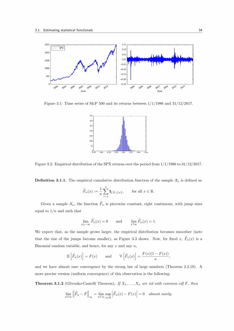
Consider for example the evolution of the S&P500 between January 1st, 1986 and August 31st
2017, and let us call si its price on day i, for i = 1, . . . , n, with n the number of trading days over
the period; here n = 7983. Define the daily log-returns1 xi := log(si/si−1), for i = 1, . . . , n − 1.
Relabelling the index so that the sample reads Xn is now of size n = 7982, we can plot both the
time series of the returns as well as their empirical distribution. Statistics’ aim is to infer from
these plots a distribution, or a model, describing the sample Xn of returns. If one assumes that
the returns are Gaussian, i.e. Xn is the realisation of some N (µ, σ2) random variable, then the
histogram should correspond (more or less) to the Gaussian density.
Exercise 10. There are two clear drops in the SPX evolution. What do they correspond to?
What kind of observations can we make from the evolution of the returns?
3.1 Estimating statistical functionals
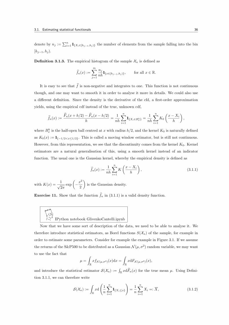
In Figure 3.1, we plotted the empirical distribution of the returns of the S&P500 over a given
period. The first question one should ask is how it is in fact plotted; the second one, in order to
be able to build some model, is to determine the shape/characteristics of this distribution.
1One may wonder why we consider logarithmic returns. Suppose that we were to consider returns of the formsi−si−1
si−1= si
si−1− 1, which is equal—up to a second-order error—to the logarithmic returns.
33
3.1. Estimating statistical functionals 34
Figure 3.1: Time series of S&P 500 and its returns between 1/1/1986 and 31/12/2017.
Figure 3.2: Empirical distribution of the SPX returns over the period from 1/1/1986 to 31/12/2017.
Definition 3.1.1. The empirical cumulative distribution function of the sample Xn is defined as
Fn(x) :=1
n
n∑i=1
11Xi≤x, for all x ∈ R.
Given a sample Xn, the function Fn is piecewise constant, right continuous, with jump sizes
equal to 1/n and such that
limx↓−∞
Fn(x) = 0 and limx↑∞
Fn(x) = 1.
We expect that, as the sample grows larger, the empirical distribution becomes smoother (note
that the size of the jumps become smaller), as Figure 3.3 shows. Now, for fixed x, Fn(x) is a
Binomial random variable, and hence, for any x and any n,
E[Fn(x)
]= F (x) and V
[Fn(x)
]=F (x)(1− F (x))
n,
and we have almost sure convergence by the strong law of large numbers (Theorem 2.2.19). A
more precise version (uniform convergence) of this observation is the following:
Theorem 3.1.2 (Glivenko-Cantelli Theorem). If X1, . . . , Xn are iid with common cdf F , then
limn↑∞
∥∥∥Fn − F∥∥∥∞
= limn↑∞
supx∈R
∣∣∣Fn(x)− F (x)∣∣∣ = 0 almost surely.

3.1. Estimating statistical functionals 35
Figure 3.3: Empirical cdf of a Gaussian N (0, 1) sample for different values of the sample size n,
together with the exact Gaussian cdf (line).
Proof. Consider the simpler case where the function F is continuous. In that case, for any integer k,
we can find a sequence −∞ = x0 < x1 < · · · < xk−1 < xk = +∞ such that F (xi) = i/k. Now, for
any x ∈ [xi−1, xi], the monotonicity of both Fn and F imply
Fn(xi−1)−F (xi−1)−1
k= Fn(xi−1)−F (xi) ≤ Fn(x)−F (x) ≤ Fn(xi)−F (xi−1) = Fn(xi)−F (xi)+
1
k,
so that ∣∣∣Fn(x)− F (x)∣∣∣ ≤ max
i=1,...,k−1
∣∣∣Fn(xi)− F (xi)∣∣∣+ 1
k
.
Since Fn(x) converges almost surely to F (x) by the strong law of large numbers (Theorem 2.2.19
applied to a sequence of iid Bernoulli trials), then
lim supn↑∞
supx∈R
∣∣∣Fn(x)− F (x)∣∣∣ ≤ 1
k,
and the theorem follows by letting k tend to infnity.
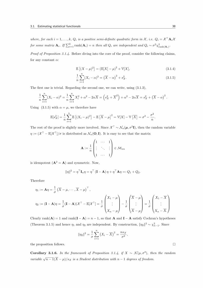
Figures 3.3 and 3.4 show convergence of the empirical densities and cumulative distribution
functions. However, at first glance, it seems that the plots of the densities are more revealing than
those of the cdfs, and one may wonder whether the Glivenko-Cantelli Theorem has an analogue
for empirical densities. We first need to define properly what an empirical density is. We follow
the intuition arising from the plots: let h = (h1, . . . , hm) be an ordered series of bins containing
the support of Xn, for some integer m, with mini=1,...,nXi ≤ h1 ≤ · · · ≤ maxi=1,...,nXi ≤ hm, and
such that the length of each interval hj − hj−1 is constant equal to h. For each j = 2, . . . ,m, we
3.1. Estimating statistical functionals 36
denote by nj :=∑n
i=1 11Xi∈[hj−1,hj) the number of elements from the sample falling into the bin
[hj−1, hj).
Definition 3.1.3. The empirical histogram of the sample Xn is defined as
fn(x) :=
m∑j=1
njnh
11x∈[hj−1,hj), for all x ∈ R.
It is easy to see that f is non-negative and integrates to one. This function is not continuous
though, and one may want to smooth it in order to analyse it more in details. We could also use
a different definition. Since the density is the derivative of the cfd, a first-order approximation
yields, using the empirical cdf instead of the true, unknown cdf,
fn(x) :=Fn(x+ h/2)− Fn(x− h/2)
h=
1
nh
n∑i=1
11Xi∈Bhx =
1
nh
n∑i=1
K0
(x−Xi
h
),
where Bhx is the half-open ball centred at x with radius h/2, and the kernel K0 is naturally defined
as K0(x) := 11−1/2<x≤1/2. This is called a moving window estimator, but is still not continuous.
However, from this representation, we see that the discontinuity comes from the kernel K0. Kernel
estimators are a natural generalisation of this, using a smooth kernel instead of an indicator
function. The usual one is the Gaussian kernel, whereby the empirical density is defined as
fn(x) :=1
nh
n∑i=1
K
(x−Xi
h
), (3.1.1)
with K(x) =1√2π
exp
(−x
2
2
)is the Gaussian density.
Exercise 11. Show that the function fn in (3.1.1) is a valid density function.
IPython notebook GlivenkoCantelli.ipynb
Now that we have some sort of description of the data, we need to be able to analyse it. We
therefore introduce statistical estimators, as Borel functions S(Xn) of the sample, for example in
order to estimate some parameters. Consider for example the example in Figure 3.1. If we assume
the returns of the S&P500 to be distributed as a Gaussian N (µ, σ2) random variable, we may want
to use the fact that
µ =
∫RxfN (µ,σ2)(x)dx =
∫RxdFN (µ,σ2)(x),
and introduce the statistical estimator S(Xn) :=∫R xdFn(x) for the true mean µ. Using Defini-
tion 3.1.1, we can therefore write
S(Xn) :=
∫Rxd
(1
n
n∑i=1
11Xi≤x
)=
1
n
n∑i=1
Xi =: X, (3.1.2)
3.1. Estimating statistical functionals 37
Figure 3.4: Empirical density of a Gaussian N (0, 1) sample for different values of the sample size n.
which is nothing else than the arithmetic average. Under general assumptions on the function S,
one can prove that the Glivenko-Cantelli Theorem 3.1.2 yields convergence of S(Fn) to S(F ) as
the sample size n tends to infinity. With the function
S(F ) :=∫x2F (dx)−
(∫xF (dx)
)2
,
the estimator is that of the variance, defined as
s2X :=1
n
n∑i=1
(Xi −X
)2=
1
n
n∑i=1
X2i −X
2, (3.1.3)
and sX is called the standard deviation. Let us summarise a few properties of these two estimators:
Proposition 3.1.4. Let X = (X1, . . . , Xn) be an iid sample with common distribution X satisfying
E[X] = µ and V[X2] = σ2 <∞, then
E[X]= µ, V
[X]=σ2
n, E
[s2X]=n− 1
nσ2.
Furthermore, the sample mean X and the sample variance s2X are independent and converge almost
surely to µ and σ2 as n tends to infinity. Finally the random variable ns2X /σ2 is distributed as a
Chi-Square distribution with n− 1 degrees of freedom.
In order to prove this proposition, recall the following theorem, due to Cochran:
Theorem 3.1.5. Let X := (X1, . . . , Xn) denote an iid sequence of N (0, σ2) random variables,
and assume thatn∑
i=1
X2i =
k∑i=i
Qi,
3.1. Estimating statistical functionals 38
where, for each i = 1, . . . , k, Qi is a positive semi-definite quadratic form in X , i.e. Qi = X⊤AiX
for some matrix Ai. If∑k
i=1 rank(Ai) = n then all Qi are independent and Qi ∼ σ2χ2rank(Ai)
.
Proof of Proposition 3.1.4. Before diving into the core of the proof, consider the following claims,
for any constant α:
E[(X − µ)2
]= (E[X]− µ)
2+ V[X], (3.1.4)
1
n
n∑i=1
(Xi − α)2 =(X − α
)2+ s2X . (3.1.5)
The first one is trivial. Regarding the second one, we can write, using (3.1.3),
1
n
n∑i=1
(Xi − α)2 =1
n
n∑i=1
X2i + α2 − 2αX =
(s2X +X
2)+ α2 − 2αX = s2X +
(X − α
)2.
Using (3.1.5) with α = µ, we therefore have
E[s2X ] =1
n
n∑i=1
E[(Xi − µ)2
]− E
[X − µ
]2= V[X]− V
[X]= σ2 − σ2
n.
The rest of the proof is slightly more involved. Since X⊤ ∼ Nn(µ, σ2I), then the random variable
η := (X⊤ − E[X⊤]/σ is distributed as Nn(O, I). It is easy to see that the matrix
A :=1
n
1 · · · 1...
. . ....
1 · · · 1
∈ Mnn
is idempotent (A2 = A) and symmetric. Now,
∥η∥2 = η⊤Inη = η⊤ (I−A) η + η⊤Aη =: Q1 +Q2.
Therefore
η1 := Aη =1
σ
(X − µ, · · · , X − µ
)⊤,
η2 := (I−A)η =1
σ(I−A)(X⊤ − E[X⊤] =
1
σ
X1 − µ
...
Xn − µ
− 1
σ
X − µ
...
X − µ
=1
σ
X1 −X
...
Xn −X.
Clearly rank(A) = 1 and rank(I−A) = n− 1, so that A and I−A satisfy Cochran’s hypotheses
(Theorem 3.1.5) and hence η1 and η2 are independent. By construction, ∥η2∥2 ∼ χ2n−1. Since
∥η2∥2 =1
σ
n∑i=1
(Xi −X
)2=nsXσ2
,
the proposition follows.
Corollary 3.1.6. In the framework of Proposition 3.1.4, if X ∼ N (µ, σ2), then the random
variable√n− 1(X − µ)/sX is a Student distribution with n− 1 degrees of freedom.
3.1. Estimating statistical functionals 39
Proof. Since√n(X − µ)/σ is a centered Gaussian distribution with unit variance, then
√n− 1
X − µ
sX=
√n(X − µ
)σ
√(n− 1)σ2
ns2X=
n√χ/(n− 1)
,
where n ∼ N (0, 1) and χ ∼ χ2n−1. Since n and χ are independent by Proposition 3.1.4, the
corollary follows immediately.
Other examples are useful in mathematical finance, in particular the empirical quantile of
order p is a key tool in risk management, to estimate portfolio losses, and abide by the Basel III
regulatory commitments2.
Definition 3.1.7. For a given random variable X with continuous and strictly increasing cdf F ,
the quantile of order p ∈ (0, 1) is the solution qp to the equation F (qp) = p.
However, if the cdf is not continuous or strictly increasing, this definition does not quite make
sense, and should be refined in the following way:
qp :=1
2
inf
F (q)>pq + sup
F (q)<p
q
. (3.1.6)
Of particular interests are the following:
• the median corresponds to the quantile of order p = 1/2;
• the quartiles corresponds to the quantiles of order p ∈ 1/4, 3/4;
• the difference q3/4 − q1/4 is called the inter-quartile interval.
Note in passing that quantiles are always well defined, as opposed to the mean and the variance.
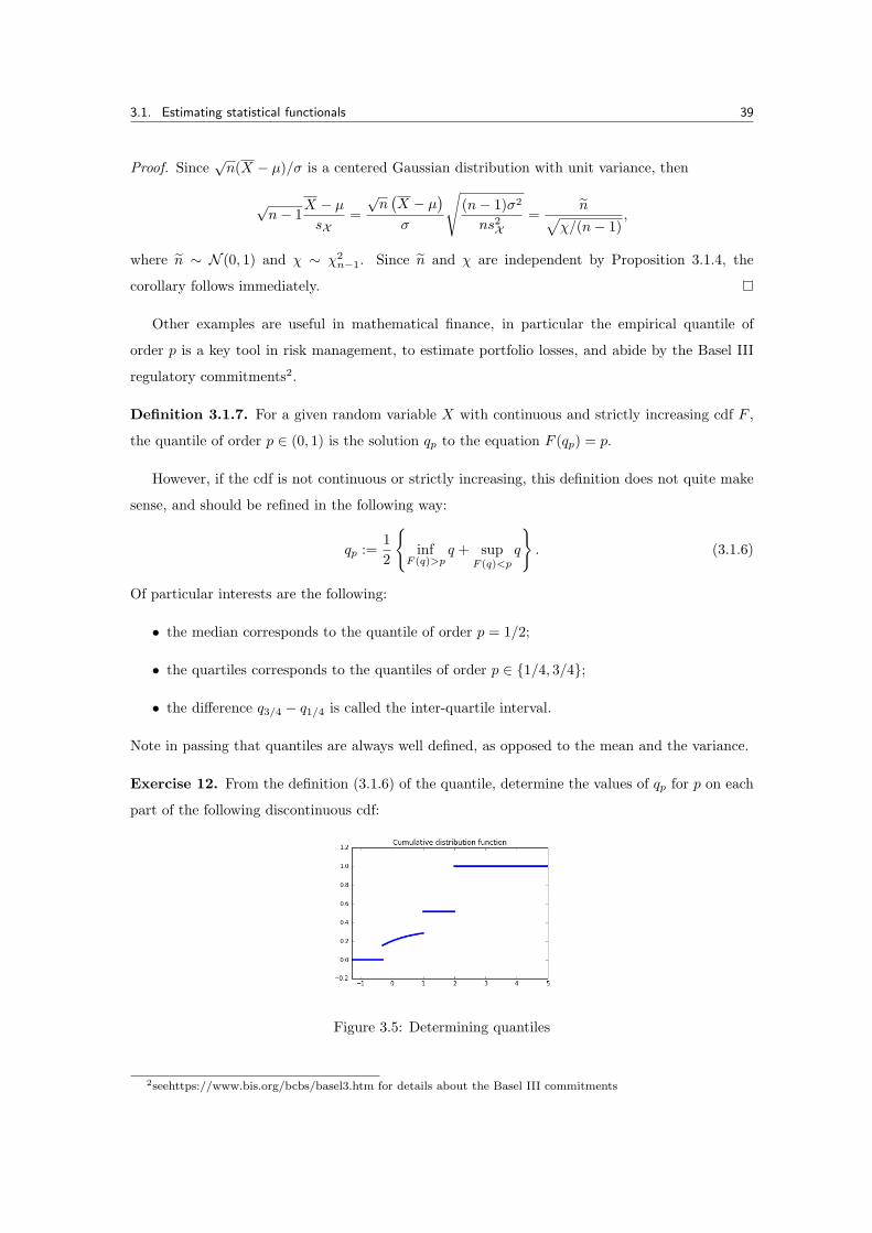
Exercise 12. From the definition (3.1.6) of the quantile, determine the values of qp for p on each
part of the following discontinuous cdf:
Figure 3.5: Determining quantiles
2seehttps://www.bis.org/bcbs/basel3.htm for details about the Basel III commitments
3.1. Estimating statistical functionals 40
From (3.1.6), we can thus define the empirical quantile of order p for the sample X as
Qn,p := S(F ) = 1
2
(inf
F (q)>pq + sup
F (q)<p
q
)
Exercise 13. By reordering the sample X in increasing order X(1) ≤ . . . ≤ X(n), show that
Qn,p =
X(k), if p ∈
(k − 1
n,k
n
),
1
2
(X(k) +X(k+1)
), if p =
k
nfor some k = 1, . . . , n.
Suppose now that we observe two samples Xn and Yn (say of two different indices, S&P500
and DAX). We can then define the empirical covariance sX ,Y and the empirical correlation ρX ,Y
between the two random vectors as
sX ,Y :=1
n
n∑i=1
(Xi −X
) (Yi − Y
)and ρX ,Y :=
sX ,Y
sX sY.
It is easy to see that |sX ,Y | ≤ 1 always holds and that sX ,Y = 1 if and only if there is a linear re-
lationship between the two samples X and Y. Note however, that a large value of |sX ,Y | does not
imply that the two theoretical random variables are linearly related. An interesting and funny
list of spurious relationships can be browsed through at http://www.tylervigen.com/spurious-
correlations.
Exercise 14. Using the convergence results above as well as the strong law of large numbers,
prove that the convergence of these two estimators to the true covariance and correlation.
Remark 3.1.8. Given some functional S(F ) of an unknown cdf, the standard way to define an
estimator thereof is to consider S(Fn).
Exercise 15. Write down an estimator for the skewness s := E[(X − E[X])3]/V[X]3/2.
Exercise 16. In an IPython notebook, import two years of daily data of two stocks in the S&P500,
compute the daily returns. From this, determine the values of the empirical mean, standard
deviation, skewness and correlation.
Remark 3.1.9. One should be careful about drawing conclusions about the theoretical random
variables from their empirical estimators. In particular very few occurrences of extreme observa-
tions can often lead to deceptive intuitions, for example, the 1987 crash. This requires tools from
Extreme Value Theory, which are outside the scope of the present lectures.
IPython notebook SPXHistory.ipynb
3.2. Statistical inference 41
3.2 Statistical inference
We considered so far the simple case of a sample of n observations of some random variable. We now
look at the general case where the sample Xn = (X1, . . . ,Xn) consists of n iid random vectors, each
real valued and of dimension p. Regarding the notations, given some (vector of) parameter(s) θ,
and some random vector X ∈ Rp, we shall write fθ the density of X, Fθ its distribution, and
correspondingly Eθ the expectation.
3.2.1 Definition of estimators
By statistical model, we shall mean here a set of distribution (or density) functions, which can be
either parameterised by some parameters or not. In the latter case, we speak of non-parametric
estimation, and we consider general classes of functions for the distribution, as in the following
examples:
Example 3.2.1 (Examples of non-parametric estimation). We consider X1, . . . , Xn independent
observations from an (unknown) cumulative distribution F , which we wish to estimate, given that
it belongs to the family F , the set of all cumulative distribution functions. Suppose now we wish
to estimate its density f = F ′. The set F is not valid as elements therein do not necessarily admit
a density. A classical set to consider for f ∈ f is
f := f0 ∩ fSOB,
where f0 denotes the set of all densities and fSOB the Sobolev space
fSOB :=
f :
∫(f ′′(x))
2dx <∞
,
which ensures that the class of densities is sufficiently smooth.
Example 3.2.2 (Further non-parametric statistical models).
• The model F = all distributions with finite first moments is non parametric.
• Consider pairs of observations ((X1, Y1), . . . , (Xn, Yn))), where X represents the predictor
and Y the outcome. We wish to consider all the possible regression functions r(x) :=
E[Y |X = x]. If the set F of such functions is finite (polynomials up to some degree), then F
is parametric; on the other hand, if F is infinite dimensional, then it is non-parametric.
We now focus on parametric estimation, and will adopt as main assumption we the fact that
the common distribution F is partially known, more specifically,
Assumption 3.2.3. The common distribution F belongs to some parametric family of distribu-
tions F = (Fθ)θ∈Θ.
3.2. Statistical inference 42
Here, θ ∈ Θ corresponds to the parameters of the distribution, for which we wish to determine
some statistical estimator. It may be the case that we are only interested in some, but not all,
parameters of a statistical model, for example if we already know the values of other parameters.
Consider for example the model F = N (µ, θ2), θ > 0, where we assume that we already know the
mean µ, and are only interested in estimating the volatility θ. Then Θ = R∗+, and the parameter µ
is called a nuisance parameter. We shall always assume the following:
Identifiability Hypothesis: two distributions in F are the same if and only if they have the
same parameters.
Mathematically, we can restate this hypothesis in the following form:
Identifiability Hypothesis: the map θ 7→ Pθ is injective.
Remark 3.2.4. The latter hypothesis may sound strange, but suppose that the statistical model F
has the form
Fθ(dx) =1√2π
exp
(x− θ2)2
2
dx, for all x ∈ R,
for θ ∈ Θ = R. Clearly, for any θ ∈ Θ, the laws Fθ and F−θ are identical, and hence uniqueness of
the parameter is compromised. This can here be circumvented by taking Θ = R+ instead though.
Remark 3.2.5. If the observed sequence cannot be assumed to be iid, then one may have to
consider the joint law of the vector (X1, . . . ,Xn) instead; the auto-regressive ARMA model is a
classical example. We shall not consider this case in these lectures, though.
Example 3.2.6. The following examples are all parametric statistical models:
• F = N (θ, σ2), θ ∈ R for some known σ > 0;
• F = N (θ1, θ22), θ1 ∈ R, θ2 > 0;
• F = P(θ), θ > 0, the set of all Poisson distributions with parameter θ3.
We shall from now on denote by θn an estimator of the real parameter θ, and, remembering
that it is indeed a random variable, call it unbiased if Eθ(θn) = θ.
Definition 3.2.7. An estimator θn is said to be (respectively strongly) consistent if it converges
to θ in probability (resp. almost surely) for all θ ∈ Θ, namely if
limn↑∞
Pθ
(∣∣∣θn − θ∣∣∣ ≥ ε
)= 0, for all ε > 0, θ ∈ Θ.
Note that if θn is a consistent estimator of θ, then so is αnθn for any sequence (αn) converging
to 1, so that the notion of consistent estimator, though fundamental, is in fact rather weak.
3Remember that the Poisson distribution X ∼ P(θ) is characterised by P(X = n) = θne−θ/(n!) for each
n = 0, 1, 2, . . ..
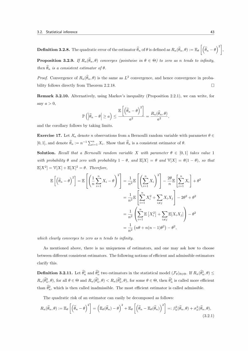
3.2. Statistical inference 43
Definition 3.2.8. The quadratic error of the estimator θn of θ is defined asRn(θn, θ) := Eθ
[(θn − θ
)2],
Proposition 3.2.9. If Rn(θn, θ) converges (pointwise in θ ∈ Θ) to zero as n tends to infinity,
then θn is a consistent estimator of θ.
Proof. Convergence of Rn(θn, θ) is the same as L2 convergence, and hence convergence in proba-
bility follows directly from Theorem 2.2.18.
Remark 3.2.10. Alternatively, using Markov’s inequality (Proposition 2.2.1), we can write, for
any a > 0,
P(∣∣∣θn − θ
∣∣∣ ≥ a)≤
E[(θn − θ
)2]a2
=Rn(θn, θ)
a2,
and the corollary follows by taking limits.
Exercise 17. Let Xn denote n observations from a Bernoulli random variable with parameter θ ∈
[0, 1], and denote θn := n−1∑n
i=1Xi. Show that θn is a consistent estimator of θ.
Solution. Recall that a Bernoulli random variable X with parameter θ ∈ [0, 1] takes value 1
with probability θ and zero with probability 1 − θ, and E[X] = θ and V[X] = θ(1 − θ), so that
E[X2] = V[X] + E[X]2 = θ. Therefore,
E[(θn − θ
)2]= E
( 1
n
n∑i=1
Xi − θ
)2 =
1
n2E
( n∑i=1
Xi
)2− 2θ
nE
[n∑
i=1
Xi
]+ θ2
=1
n2E
n∑i=1
X2i +
∑i =j
XiXj
− 2θ2 + θ2
=1
n2
n∑i=1
E[X2
i
]+∑i =j
E[XiXj ]
− θ2
=1
n2(nθ + n(n− 1)θ2
)− θ2,
which clearly converges to zero as n tends to infinity.
As mentioned above, there is no uniqueness of estimators, and one may ask how to choose
between different consistent estimators. The following notions of efficient and admissible estimators
clarify this.
Definition 3.2.11. Let θ1n and θ2n two estimators in the statistical model (Fθ)θ∈Θ. If Rn(θ1n, θ) ≤
Rn(θ2n, θ), for all θ ∈ Θ and Rn(θ
1n, θ) < Rn(θ
2n, θ), for some θ ∈ Θ, then θ1n is called more efficient
than θ2n, which is then called inadmissible. The most efficient estimator is called admissible.
The quadratic risk of an estimator can easily be decomposed as follows:
Rn(θn, θ) := Eθ
[(θn − θ
)2]=(Eθ(θn)− θ
)2+ Eθ
[(θn − Eθ(θn)
)2]=: β2
n(θn, θ) + σ2n(θn, θ),
(3.2.1)
3.3. Parametric inference 44
Figure 3.6: Convergence of the empirical mean and variances as estimators for the mean and the
variance in the N (0, 1) case.
where βn is called the bias and σ2n the variance of the estimator θn, so that θn is unbiased if
βn(θn, θ) = 0 for all θ ∈ Θ. The following classical exercise illustrates several far-reaching issues:
Exercise 18. Consider the statistical model F = N (0, σ2), σ ∈ R∗+, and define the following
two estimators of the true variance σ2:
θ1n :=1
n
n∑i=1
(Xi −X
)2and θ2n :=
1
n− 1
n∑i=1
(Xi −X
)2.
Show that θ1n is biased while θ2n is not, and compare their quadratic risks.
Solution. From Proposition 3.1.4, noticing that θ1n is in fact the same as s2X , we immediately
obtain that it is biased, but that θ2n is not, and the bias of θ1n reads
Eσ(θn)− σ2 =n− 1
nσ2 − σ2 = −σ
2
n.
We can further compute the variances of the estimators as
Eσ
[(θ1n − Eσ(θ
1n))2]
=2(n− 1)σ4
n2and Eσ
[(θ2n − Eσ(θ
2n))2]
=2σ4
n− 1,
and therefore, the quadratic risks read
Rn(θ1n, σ
2) =
(σ2
n
)2
+2(n− 1)σ4
n2=
2n− 1
n2σ4 and Rn(θ
2n, σ
2) =2σ4
n− 1,
as well as the inequality Rn(θ2n, σ
2) > Rn(θ1n, σ
2), meaning that the estimator θ1n, despite being
biased, is in fact more efficient while θ2n is inadmissible.
3.3 Parametric inference
3.3.1 The method of moments
We are interested here in estimating the moments of the law generating a given sample X1, . . . , Xn.
Following the terminology above, the common law of the sample is drawn from the statistical model
3.3. Parametric inference 45
F = (Fθ)θ∈Θ. Define
µr(θ) := Eθ(Xr) =
∫RxrFθ(dx), (3.3.1)
the moment of order r for Fθ, which we assume to exist for all r ≤ q, for some integer q. However,
these moments are not known since they depend on the unknown parameter θ. We therefore
consider their empirical estimators
mr :=1
n
n∑i=1
Xri ,
which we know converge to the true value as the sample size n tends to infinity. The following
method is due to Pearson 4.
Definition 3.3.1. In the statistical model F , the method of moments estimator θMMn for θ is the
solution to the system
µr
(θMMn
)= mr, for r = 1, . . . , q.
Exercise 19.
• Let F = N (µ, σ2), µ ∈ R, σ ∈ R∗+. Show that the estimators (3.1.2) and (3.1.3) correspond
to method of moment estimators.
• Compute the method of moment estimator for the parameter of the exponential distribution
using the first two moments.
3.3.2 The generalised method of moments
Instead of the moments µr, one could consider more general functions, rewriting (3.3.1) as
µr(θ) := Eθ(ϕr(X)),
for a general family of functions (ϕr)r=1,...,q, and we replace their estimators by
mr :=1
n
n∑i=1
ϕr(Xi).
We also denote by θGMn the corresponding generalised method of moment estimator. The reason
for introducing this generalised method is that moments may not exist for some distribution,
and functions other than polynomials may help circumventing this issue. Consider the Cauchy
distribution, the density of which is given by
Fθ(dx) =1
π
dx
1 + (x− θ)2 , for all x ∈ R.
4Karl Pearson (1857-1936) was an English mathematician, and is one of the founders of mathematical statistics.
His contributions are fundamental and widely spread, in particular the method of moments, Principal Component
Analysis, the correlation coefficient, the histogram, and the p-value.
3.3. Parametric inference 46
Exercise 20.
• Show that no moment exists.
• With the function ϕ1(x) := sgn(x) = 11x>0 − 11x≤0, show that the generalised method of
moments estimator θGMn , given a sample Xn, is of the form
θGMn = tan
(π
2n
n∑i=1
sgn(Xi)
).
• Show that θGMn is a consistent estimator and that it is asymptotically Gaussian, i.e. that
√n(θGMn − θ∗
)converges in distribution to a centered Gaussian random variable with vari-
ance to determine explicitly.
3.3.3 The Delta method
The Delta method is in fact another way of understanding the generalised method of moments:
assume that, from the observations, one can construct an estimator of the form φ(θ). If the
function φ is sufficiently smooth, then an estimator of θ can be obtain taking the reciprocal φ−1.
Let us state this more formally:
Theorem 3.3.2. Consider the iid sample (X1, . . . , Xn) with common law Pθ, for θ ∈ Θ ⊂ R, and φ
a C1(Θ → φ(Θ))-diffeomorphism. If φn = φn(X1, . . . , Xn) is a convergent estimator of φ(θ), and θ
an interior point of Θ, then θn = φ−1 (φn) is defined almost surely as n tends to infinity and θn
converges in probability to θ. Furthermore, if there exists a sequence (α)n diverging to infinity and
a random variable Zθ such that
αn (φn − φ(θ)) converges in law to Zθ,
then
αn
(θn − θ
)converges in law to
Zθ
φ′(θ).
Remark 3.3.3. The classical example is when α = n−1/2 and Zθ ∼ N (0, σ2θ).
Proof. First note that since the sequence (αn (φn − φ(θ)))n converges in law to Zθ, then (φn)n
converges in probability to φ(θ). Now, because θ belongs to the interior of Θ and φ is bijective and
continuous, then φ(θ) belongs to the interior of φ(Θ). Furthermore, since (φn)n converges to φ(θ)
in probability, then
limn↑∞
P (φn ∈ φ(Θ)) = 1.
Let ψ ≡ φ−1 be the inverse function; by assumption, the Taylor expansion around the point φ(θ)
ψ(x) = ψ(φ(θ)) + (x− φ(θ)) [ψ′(φ(θ)) + ε(x)]
3.3. Parametric inference 47
holds, where ε(x) tends to zero as x approaches φ(θ). Since (φn)n converges in probability, then,
by continuity, so does ψ(φn), and we can write the (random) expansion
ψ(φn) = ψ(φ(θ)) + (φn − φ(θ)) [ψ′(φ(θ)) + ε(φn)] ,
where the sequence (ψ′(φ(θ))+ε(φn))n converges in probability to ψ′(φ(θ)), and the result follows
from Slutsky’s theorem. We just recall in passing the useful identity:
ψ′(y) =1
(φ′ φ) (y)=⇒ ψ′ (φ(θ)) =
1
φ′(θ).
Example 3.3.4 (Sample variance). Using previous notations, the sample variance of the iid sample
X = (X1, . . . , Xn is defined in (3.1.3) as
s2X =1
n
n∑i=1
X2i −X
2=: φ
(X,X2
),
where φ(x, y) := y − x2. Assume that s2X is computed from a sample of a distribution with finite
first four moments µ1, . . . , µ4. The Central Limit Theorem implies that
√n
X
X2
−
µ1
µ2
converges in distribution to N =
N1
N2
∼ N
0
0
,
µ2 − µ21 µ3 − µ1µ2
µ3 − µ1µ2 µ4 − µ22
.
Clearly, the function φ is differentiable at θ = (µ1, µ2)⊤ with gradient equal to (−2µ1, 1). Therefore
√n(φ(X,X2
)− φ(µ1, µ2)
)converges in distribution to − 2µ1N1 +N2
3.3.4 Maximum likelihood method
We now move on to one of the most important and most widely used estimation method, namely
Maximum Likelihood Estimation, popularised by Fisher5 in the 1920s. In order to use this method,
we need to assume that the statistical model F admits a density with respect to the Lebesgue
measure, which we denote by fθ for each θ ∈ Θ.
Definition 3.3.5. The maximum likelihood function is the map Ln from Θ to R defined as
Ln(θ) :=n∏
i=1
fθ(Xi), for all θ ∈ Θ,
and the function ln := − 1n logLn is called the log-likelihood.
When the sequence of observations (X1, . . . , Xn) is assumed to be iid, note that the maximum
likelihood function is nothing else than the joint density of the sample.
5Ronald Fisher (1890-1972) was an English statistician and geneticist. He is vastly regarded as one of the founders
of modern statistics, and of population genetics
3.3. Parametric inference 48
Definition 3.3.6. The maximum likelihood estimator is defined as
θMLn := argmax
θ∈ΘLn(θ).
It is clear that we can also write θMLn := argminθ∈Θ ln(θ), and that a necessary condition is
that the gradient of either ln or Ln is null, and we call
∇ln(θ) = 0 (3.3.2)
the likelihood equation (or likelihood system). Note that existence of a maximum likelihood esti-
mator is not necessarily linked to that of a root to (3.3.2).
Example 3.3.7. [Maximum Likelihood Estimator for the Gaussian distribution] For the Gaussian
statistical model F = N (µ, σ2), µ ∈ R, σ > 0, we can write
Ln(θ) =(σ√2π)−n
exp
(− 1
2σ2
n∑i=1
(Xi − µ)2
),
ln(θ) =log(2π)
2+ log(σ) +
1
2nσ2
n∑i=1
(Xi − µ)2.
The likelihood system ∇ln(θ) = 0 is therefore equivalent to
∂µln(θ) = 0,
∂σln(θ) = 0if and only if
n∑
i=1
(Xi − µ) = 0,
n∑i=1
(Xi − µ)2 = σ2n,
so that
µ = X and σ =
(1
n
n∑i=1
(Xi −X
)2)1/2
= sX .
Example 3.3.8 (Maximum Likelihood Estimator for the Uniform distribution). Consider the
Uniform distribution on the closed interval [0, θ], with density given by fθ(x) = θ−111[0,θ](x). The
likelihood function is then given by
Ln(θ) :=n∏
i=1
fθ(Xi) =1
θn
n∏i=1
11[0,θ](Xi) =1
θn11[maxi=1,...,n Xi,∞)(θ), for all θ ∈ Θ.
It is clear that the maximum of the function is then attained at the point θMLn = max
i=1,...,nXi. This
estimator has many immediate properties; in particular, P(θMLn ≤ t) = (t/θ)n for any t ∈ [0, θ] and
its density and expectation therefore read
fθMLn
(t) =n
θntn−111[0,θ](t) and E
[θMLn
]=
nθ
n+ 1.
It is biased, and we can compute directly its second moment and its quadratic risk as
E[(θMLn
)2]=
nθ2
n+ 2and R
(θMLn , θ
)=
2θ2
(n+ 1)(n+ 2).
3.3. Parametric inference 49
Asymptotic behaviour of the log-likelihood function
In this section, we shall denote by θ∗ the true value of the parameter, and will consider the following
standing assumption:
Assumption 3.3.9. For any θ ∈ Θ,∫| log fθ(x)|Fθ∗(dx) is finite.
Under this assumption, it is easy to see that the parameterised sequence (Zθi )i=1...,n defined by
Zθi := − log fθ(Xi) is iid with
E[Zθi
]= −
∫log fθ(x)fθ∗(x)dx =: J(θ). (3.3.3)
The function J is called the contrast (or divergence) function, and corresponds exactly, by the law
of large numbers, to the limit in probability of the log-likelihood function. This link, together with
the following lemma, justifies fully the maximum likelihood method.
Lemma 3.3.10. Under Assumption 3.3.9, the inequality J(θ) ≥ J(θ∗) holds for all θ ∈ Θ. Fur-
thermore, under the Identifiability Hypothesis, the inequality is strict whenever θ = θ∗.
Proof. By convexity of the logarithm, the inequality log(1 + z) − z ≤ 0 holds for all z ≥ −1, and
is an equality if and only if z = 0. Therefore, for any x, θ, we can write
log
(fθ(x)
fθ∗(x)
)−(fθ(x)
fθ∗(x)− 1
)= log
(1 +
[fθ(x)
fθ∗(x)− 1
])−(fθ(x)
fθ∗(x)− 1
)≤ 0.
Since ∫ (fθ(x)
fθ∗(x)− 1
)fθ∗(x)dx = 0,
we therefore obtain
J(θ)−J(θ∗) = −∫fθ∗(x) log
(fθ(x)
fθ∗(x)
)dx = −
∫fθ∗(x)
log
(fθ(x)
fθ∗(x)
)−(fθ(x)
fθ∗(x)− 1
)dx ≥ 0.
Noting that the inner bracket is non-positive, it therefore has to be null on the set A := x :
fθ∗(x) > 0. By convexity of the logarithm, though, this is true if and only if fθ(x)/fθ∗(x) = 1
almost surely on A, which implies fθ(x) = fθ∗(x) almost surely for all x. Summarising, we have
J(θ) = J(θ∗) if and only if fθ(x) = fθ∗(x) almost surely for all x, and the Identifiability Hypothesis
yields θ = θ∗, and the lemma follows.
Consistency of the maximum likelihood estimator
We saw above several types of estimators, which may or may not be consistent. In particular, in
the case where F = N (θ, 1), θ ∈ R, the maximum likelihood estimator θMLn corresponds exactly
to the empirical average X whereas the real value is the theoretical mean which, in general, is
different. The following theorem gathers a set of sufficient conditions ensuring that they are the
same.
3.3. Parametric inference 50
Theorem 3.3.11. If the following conditions hold:
1. Θ is an open subset of R,
2. the Identifiability Hypothesis holds,
3. for any x ∈ R, the function θ 7→ fθ(x) is continuous on Θ,
4. Assumption 3.3.9 holds,
5. θMLn exists for all n and the local minima of ln forms a closed bounded set in the interior of Θ,
then the maximum likelihood estimator is consistent.
3.3.5 Bayes estimators
We finish this review of estimators by Bayes estimators, which essentially relies on a generalised
notion of the risk associated to an estimator (we so far only saw quadratic risk in Definition 3.2.8).
We keep the same framework as before, and introduce a so-called loss function λ : Θ × Θ → R+
and the associated risk function
Rλ(θ, θ) := Eθ
[λ(θ, θ)]
=
∫Rn
λ(θ, θ)Pθ(dx), for all θ ∈ Θ,
where θ is a given estimator. The motivation for Bayes estimation is the following issue: consider
the Gaussian statistical model F = N (θ, 1), θ ∈ R, and, from a Gaussian N (θ, 1) sample, we
consider the Maximum Likelihood estimator θMLn as well as the constant estimator θ = 0. The
quadratic risk, corresponding to the loss function λ(x, y) = (x− y)2, can be computed as (we shall
use the notation RQ for the quadratic risk here)
RQ(θ, θML
n
)= V
[X]=
1
nand RQ
(θ, θ)= θ2. for any θ ∈ Θ.
Therefore, the maximum likelihood estimator is better only when RQ(θ, θML
n
)< RQ
(θ, θ), that
is when |θ| > n−1/2, which is awkward since we do not actually know the value of θ. Bayes’
paradigm is to endow θ with some distribution µ, supported on Θ, accounting for this uncertainty.
Definition 3.3.12. The Bayesian risk with the law µ, for some estimator θ, is defined as
RλB
(µ, θ):=
∫Θ
Rλ(θ, θ)µ(dθ) =
∫Θ
(∫Rn
λ(θ, θ)Pθ(dx)
)µ(dθ)
Example 3.3.13. In the framework of the Gaussian estimation above, consider µ = N (0, 1). Then
RQB
(µ, θML
n
):=
∫Θ
RQ(θ, θML
n
)µ(dθ) =
∫R
µ(dθ)
n=
1
n,
RQB
(µ, θ)
:=
∫Θ
RQ(θ, θ)µ(dθ) =
∫Rθ2µ(dθ) = 1,
3.3. Parametric inference 51
so that, in the Bayesian sense, the Maximum Likelihood estimator is better than the constant one.
Note that, in fact, for any square integrable prior distribution µ, the Bayesian quadratic risk for the
maximum likelihood estimator will always be equal to 1n , whereas it will be equal to some constant
for the trivial estimator, and hence the MLE will be better for large enough sample size n.
The following definition is the Bayes’ equivalent of the maximum likelihood estimator. Given
the observation X , we shall call f(θ|X ) the posterior density, namely the density of θ conditional
on the observation X . Recall Bayes’ formula:
f(θ|x) = f(x|θ)f(θ)f(x)
=f(x|θ)f(θ)∫
Θf(x|τ)f(τ)dτ
. (3.3.4)
Definition 3.3.14 (Bayes Estimator). For a given prior distribution µ, the Bayes estimator θB is
defined as
θB(x) := argminτ∈Θ
E [λ(θ, τ)|X = x] = argminτ∈Θ
∫Θ
λ(θ, τ)f(θ|x)dθ.
Exercise 21. Show that, with the quadratic loss function λ(x, y) = (x− y)2, the Bayes estimator
is simply the conditional expectation θB(x) = E [θ|X = x].
Solution. Let Φx(τ) :=
∫Θ
λ(θ, τ)f(θ|x)dθ =
∫Θ
(θ − τ)2f(θ|x)dθ the function to be minimised,
which does not depend on θ, with x as a parameter. Then, by Leibniz integral rule,
∂τΦx(τ) = ∂τ
∫Θ
(θ − τ)2f(θ|x)dθ =∫Θ
∂τ[(θ − τ)2f(θ|x)
]dθ
= −2
∫Θ
(θ − τ)f(θ|x)dθ = −2
∫Θ
θf(θ|x)dθ + 2τ
∫Θ
f(θ|x)dθ
= −2 (E [θ|X = x]− τ) ,
which is equal to zero if and only if τ = E [θ|X = x], and the result follows.
Exercise 22. Compute the Bayes estimator for the loss function λ(x, y) = |x− y|.
Example 3.3.15. Consider µ ∼ N (0, 1) and, knowing θ, the iid sample X is distributed according
to N (θ, 1), that is
f(x|θ) = 1
(2π)n/2exp
−1
2
n∑i=1
(xi − θ)2
Using Bayes’ formula (3.3.4), the posterior density of θ reads
f(θ|x) = 1
f(x)
1
(2π)n/2exp
−1
2
n∑i=1
(xi − θ)2
1√2π
exp
−θ
2
2
∝x exp
−n+ 1
2
(θ − nx
n+ 1
)2,
where the symbol ∝x means that the two sides are equal up to a constant multiple of x, independent
of θ. Since a density has to integrate to unity, we do not need to compute the constant to conclude
3.3. Parametric inference 52
that the law of θ conditional on X = x is Gaussian with mean nxn+1 and variance 1
n+1 . The Bayes
estimator for the quadratic risk is therefore nn+1Xn. It is biased and different from the maximum
likelihood estimator Xn, but the difference becomes negligible as the sample size increases. Since
V[θB(x)
]=
n
(n+ 1)2<
1
n= V
[θMLn
],
the quadratic risks can be computed as
RQ(θ, θB(x)
)=
n+ θ2
(n+ 1)2and RQ
(θ, θML
n
)=
1
n,
and their comparison again depends on the position of θ with respect to n. In the Bayesian
framework, if we integrate with respect to the distribution of θ, we obtain
RQB
(θ, θB(x)
)=
∫Θ
R(θ, θB(x)
)µ(dθ) =
∫R
n+ θ2
(n+ 1)2µ(dθ) =
1
n+ 1,
and
RQB
(θ, θML
n
)=
∫Θ
R(θ, θML
n
)µ(dθ) =
∫R
1
nµ(dθ) =
1
n,
so the the Bayes estimator is slightly better.
3.3.6 Regular statistical models
We consider in this section only the one-dimensional case where Θ is a subset of the real line,
i.e. we only estimate one parameter of the common distribution. We further assume that the
density fθ exists and is smooth, and define the function lθ := log fθ.
Definition 3.3.16. The Fisher information is the function I : Θ → R+ defined as
I(θ) :=
∫(∂θlθ(x))
2fθ(x)dx =
∫x:fθ(x)>0
(∂θfθ(x))2
fθ(x)dx = Eθ
[(∂θlθ(x)
2)]
In order to avoid degenerate situations, we shall work under the following set of assumptions:
Assumption 3.3.17 (Regularity Hypotheses).
• Θ is an open subset of R;
• for all x, the functions fθ and lθ are smooth;
• for any θ ∈ Θ, there exists a ball Bθ around θ and a function Λ such that, for all x,
max∂θθlθ(x), ∂θlθ(x), |∂θlθ(x)|2
≤ Λ(x) and
∫Λ(x) sup
θ∈Bθ
fθ(x)dx <∞;
• I(θ) > 0 for all θ ∈ Θ.
These regularity assumptions are not always met though, as the following examples show:
3.3. Parametric inference 53
Example 3.3.18. Consider the exponential law with parameter θ ∈ Θ = (0,∞), for which the
density reads fθ(x) = θ exp(−θx)11x>0, so that
• for any x > 0, the map θ 7→ fθ(x) is smooth on Θ;
• for any θ ∈ Θ, the map
x 7→ (∂θfθ(x))2
fθ(x)11fθ(x)>0 =
(1− θx)2
θe−θx
is integrable on R+ and
I(θ) =1
θ2Eθ
[(1− θX)2
]=
1
θ2
is continuous on Θ.
Exercise 23.
• For the uniform distribution on [0, θ] (with θ > 0), the function lθ is not differentiable;
• Consider the statistical model N (θ2, 1), θ ∈ Θ, with Θ = [0,∞); Show that I(0) = 0, so
that the model is not regular. Show that the model is regular, however, if Θ = (0,∞).
The following lemma provides an alternative characterisation of the Fisher information. Its
proof relies on integration by parts and the Fubini theorem, all justified by the regularity assump-
tions above. We recall that the divergence function J(·) was defined in (3.3.3).
Lemma 3.3.19. For a regular model, the following equalities hold:
I(θ) = −∫∂θθlθ(x)fθ(x)dx, for all θ ∈ Θ,
J(θ∗) = 0,
∂θθJ(θ∗) = −Eθ [∂θθlθ(X, θ
∗)] .
The lemma in particular implies that I(θ∗) = J ′′(θ∗), which can be used as a geometric inter-
pretation of the Fisher information based on the observed curvature of the function J around its
minimum θ∗.
Definition 3.3.20. For any θ ∈ Θ, the quantity K(θ, θ∗) := J(θ)− J(θ∗) is called the Kullback-
Leibler divergence [27] (or relative entropy) between the two distributions Fθ and Fθ∗ . Furthermore,
the quantity J(θ∗) is called the Shannon6 entropy, and is a key tool in information theory.
Theorem 3.3.21. For a regular model, the sequence√n(θMLn − θ∗
)converges in distribution to
N (0, 1/I(θ∗)) for any θ∗ ∈ Θ as n tends to infinity.
6Claude Shannon (1916-2001) was an American mathematician and electrical engineer, and the father of infor-
mation theory.
3.3. Parametric inference 54
Proof. Since θMLn is a solution to the likelihood equation, we have ∂θlθ
(θMLn
)= 0, so that
−∂θlθ(θ∗) = ∂θlθ
(θMLn
)−∂θlθ(θ∗) =
(θMLn − θ∗
)∫ 1
0
∂θθ
(uθML
n + (1− u)θ∗)du =: cn
(θMLn − θ∗
).
Now,√n∂θlθ(θ
∗) =1√n
n∑i=1
∂θlθ (Xi, θ∗) =
1√n
n∑i=1
Zi,
where the sequence (Z1, . . . , Zn) is iid with mean zero and variance I(θ∗). The Central Limit The-
orem therefore implies that the sequence (√n∂θlθ(θ
∗))n>0 converges in distribution to N (0, I(θ∗))
as n tends to infinity. We can further show–with more involved computations–that the se-
quence (cn)n>0 converges to I(θ∗) as n tends to infinity, but in probability, and the result follows
by standard combinations of probabilistic limits.
3.3.7 Comments about estimators and bias
We gather here some thoughts and comments, wrapping up some ideas from the previous sections.
Note first that, for two given estimators θ and θ, we can have R(θ, θ) < R(θ, θ) for some θ ∈ Θ,
and the reverse inequality for other values of θ, which leaves some uncertainty about the choice of
the estimator. The Bayesian framework endows θ with a distribution supported on Θ and allows,
in some cases, to discard trivial estimators. However, the choice of the prior distribution might be
debatable, and different choices may yield different answers. A general principle, however, relies
on the decomposition (3.2.1), stating that a good estimator requires both small bias and small
variance.
Regarding the bias, one should not be obsessively focussed on it, as, first a biased estimator
may be better in the sense of quadratic risk, but also there may not exist any such estimators
sometimes. Consider for example the case of an iid sample X = (X1, . . . , Xn) distributed according
to a Binomial distribution X ∼ B(n, θ) for θ ∈ Θ = (0, 1), and assume that there exists an unbiased
estimator θ(X ). Therefore, for any θ ∈ Θ, we can write
1
θ= Eθ
[θ(X )
]=
n∑k=0
θ(k)P(X = k) =
n∑k=0
θ(k)
(n
k
)θk(1− θ)n−k.
Since all the terms θ(k) are coefficients independent of θ, then we can rewrite this equality as
1
θn+1−
n∑k=0
θ(k)
(n
k
)(1
θ− 1
)n−k
= 0.
This is a polynomial in 1/θ of order n+ 1, so only admits at most n+ 1 roots. Since this equality
has to be valid for all θ ∈ Θ, we therefore conclude that no unbiased estimator actually exists.
3.4. Hypothesis testing 55
Stability
Furthermore, suppose a given unbiased estimator θ exists, and φ is a smooth strictly convex
function. Then Jensen’s inequality implies that the inequality
E[φ(θ)]
> φ(E[θ])
= φ(θ),
so that φ(θ) is biased, even though θ is not.
Parallelisation
Now, usually, the bias (if any) is of order O(1/n), and so is the variance (you can check in all the
previous examples), so that, in light of the decomposition (3.2.1) of the quadratic risk, the bias is
in fact negligible. Suppose now that we have one unbiased estimator θ and a biased one θ, with
bias bn := E[θ] − θ = O(1/n). The sample size n might be large, but we have in fact access to
many computer cores or many computers. Let N :=√n and consider thus N cores, each treating
a subset of the sample of size N . We denote by θ(1)N , . . . , θ
(N)N the partial estimators (assumed iid),
computed on each core, and define the final estimator as
τN :=1
N
N∑i=1
θ(i)N .
Then
E [τN ] = bN (θ), V [τN ] = σ2N (θ), RQ (θ, τN ) = bN (θ)2 +
σ2N (θ)
N.
Likewise,
E [τN ] = 0, V [τN ] = s2N (θ), RQ (θ, τN ) =s2N (θ)
N.
If bN (θ) = b(θ)/N , σ2N (θ) = σ2(θ)/N s2N (θ) = s2(θ)/N , then
RQ (θ, τN ) =b(θ)2 + σ2(θ)
Nand RQ (θ, τN ) =
s2(θ)
N.
Depending on the sign of b(θ)2 + σ2(θ)− s2(θ), one estimator prevails above the other.
3.4 Hypothesis testing
We now wish to construct a methodology to differentiate two possible scenarios from the data.
The standard set-up is to consider the null hypothesis H0 versus the alternative hypothesis H1,
corresponding to two disjoint sets Θ0 and Θ1 of the parameter space:
H0 : θ ∈ Θ0 versus H1 : θ ∈ Θ1. (3.4.1)
Starting from a given sample Xn, the rejection region R allows to retain or reject the hypothesis
based on the range of outcomes of Xn, in the sense that, if Xn ∈ R, thenH0 is rejected, otherwiseH0
3.4. Hypothesis testing 56
cannot be rejected. Regarding the terminology, a hypothesis of the form Θ0 = θ0 is called simple,
and the corresponding test is one-sided; a hypothesis of the form Θ0 = θ > θ0 is called composite,
and the test is two-sided. There are two types of errors pertaining to hypothesis testing. Type I
errors occur when the test rejects H0 while it is actually true; Type II errors occur when the test
keep H0 while H1 is true.
Example 3.4.1. Consider the trivial, yet motivating, example of a statistical model F = N (θ, 1), θ ∈
Θ, with Θ = 0, 1. Given a sample Xn = (X1, . . . , Xn), we consider the two sets Θ0 = 0 and
Θ1 = 1, and the corresponding hypotheses H0 and H1 in (3.4.1). Since the empirical mean Xn
is a good estimator of the true value for a large enough sample, we could consider the following
test: reject H0 if Xn > 1/2, so that the rejection region reads
R =
Xn : Xn >
1
2
.
Note that here, both the null and the alternative hypotheses are simple.
3.4.1 Simple tests
In simple hypothesis testing Θ0 = θ0 and Θ1 = θ1, we can write these two types of errors as
Type I Error: Pθ0(Xn ∈ R),
Type II Error: Pθ1(Xn /∈ R).(3.4.2)
The goal of any test is obviously to minimise the error. However, in order to minimise the Type I
error, one needs to consider a small rejection region R, which in turn is going to yield a large
Type II error, so some balance needs to be set between the two. The idea is to set an acceptable
threshold for the error, as follows:
Definition 3.4.2. The power function β(·) and the level α ∈ (0, 1) of a test with rejection region R
are defined as
β(R) := Pθ1(Xn ∈ R) and Pθ0 (Xn ∈ R) ≤ α.
If Pθ0 (Xn ∈ R) = α, then α is called the size of the test.
In order to simplify the terminology, we shall call a test with rejection region R and R-test
from now on.
Definition 3.4.3. For a given level α, an R∗-test with level α is called the most powerful test if
β(R∗) ≥ β(R) for any R-test of level α.
The higher the power function the lower the Type II error, with a given bound on the Type I
error. There are many such hypothesis tests in the literature, including the Wald test (which
3.4. Hypothesis testing 57
assumes that θ is asymptotically Gaussian), and the Neyman-Pearson test, which we present now.
Define a rejection region of the form
R := Xn : Rn > c , (3.4.3)
for some c > 0, where Lθ(Xn) :=∏n
i=1 fθ(Xi) denotes the likelihood function, and Rn :=Lθ1(Xn)
Lθ0(Xn)is a random variable called the likelihood ratio.
Theorem 3.4.4. [Neyman-Pearson Lemma] Let α ∈ (0, 1). If there exists c∗ > 0 such that
Pθ0 (Rn > c∗) = α, then the test is the most powerful test of level α.
Proof. Proving the theorem is equivalent to showing that for all rejection region R such that
Pθ0(Xn ∈ R) ≤ α, then Pθ1(Xn /∈ R) ≥ Pθ1(Xn /∈ R∗), or else β(R) ≤ β(R∗), where we denote R∗
the optimal rejection region corresponding to the optimal value of c∗ in the theorem. Now,
Pθ1(Xn ∈ R∗)− Pθ1(Xn ∈ R) =
∫R∗
Lθ1(x)dx−∫RLθ1(x)dx =
(∫R∗\R
−∫R\R∗
)Lθ1(x)dx.
Since R∗ \ R ⊂ R∗, then Rn > c∗ on this set, and obviously Rn ≤ c∗ on R \R∗. Therefore,(∫R∗\R
−∫R\R∗
)Lθ1(x)dx ≥ c∗
(∫R∗\R
−∫R\R∗
)Lθ0(x)dx
= c∗(∫
R∗−∫R
)Lθ0(x)dx
= c∗ [Pθ0 (Xn ∈ R∗)− Pθ0 (Xn ∈ R)] .
By assumption, Pθ0 (Xn ∈ R) ≤ α and Pθ0 (Xn ∈ R∗) = α, therefore, the right-hand side of the
last inequality is non negative, and the theorem follows.
We now introduce one of the key concepts in hypothesis testing, called the p-value, which we
shall denote by π0:
Definition 3.4.5. Consider a test of size α ∈ (0, 1) and corresponding rejection region Rα. The
p-value π0 is defined as the smallest level at which the null hypothesis can be rejected, i.e.
π0 := inf α : Xn ∈ Rα .
Clearly the possible range of values is (0, 1). When the p-value is below 1%, then there is very
strong evidence that the null hypothesis should be rejected; the range (1%, 5%) represents strong
evidence, (5%, 10%) weak evidence, and when the p-value is greater than 10%, then the test is
inconclusive, in the sense that we cannot decently reject the null hypothesis.
Example 3.4.6. We consider again the statistical model F = N (θ, σ2), θ ∈ Θ, where the
variance σ2 is known, and we consider
H0 : θ ∈ Θ0 = 0 versus H1 : θ ∈ Θ1 = 1.
3.4. Hypothesis testing 58
The likelihood function reads (see Example 3.3.7)
Lθ(Xn) =(σ√2π)n n∏
i=1
exp
− (Xi − θ)2
2σ2
,
and hence the likelihood ratio can be computed as
Rn =Lθ1(Xn)
Lθ0(Xn)= exp
n
2σ2
(2X − 1
).
The rejection region (3.4.3) therefore reads explicitly
R =exp
n
2σ2
(2X − 1
)≥ c=X > c
, (3.4.4)
for some c > 0 with c = 12 + σ2
n log(c). To choose c, we equate Pθ0(Xn ∈ R) = α = Pθ0(X ≥ c).
Since the sample is Gaussian N (0, σ2) under the null hypothesis, then X ∼ N (0, σ2
n ), and therefore
cα =σ√nΦ−1(1− α) =
σ√nq1−α. (3.4.5)
To compute the power of the test, we can write
Pθ1 (Xn ∈ R) = Pθ1
(X > c
)= Pθ1
(N (0, 1) >
(c− θ1)√n
σ
)= 1− Φ
((c− θ1)
√n
σ
).
Recall now that the p-value π0 of a test is, for a given fixed sample, the largest value of α such
that the null hypothesis H0 is not rejected. From (3.4.4), for a given level α, the rejection region
is of the form R = Rα =X > cα
, with cα given in (3.4.5), or equivalently
1− α = Φ
(√ncασ
).
Therefore, for a given X, the threshold from accepting H0 to rejecting it is α∗(X) such that
cα = X, i.e.
1− α∗(X) = Φ
(√ncασ
)= Φ
(√nX
σ
),
and therefore the critical (p-value) threshold is equal to
π0 = α∗(X) = 1− Φ
(X√n
σ
).
3.4.2 Composite tests
We now consider composite tests, that is tests of the form Θ0 = θ > θ0 versus Θ1 = θ ≤ θ0.
We slightly modify the definitions of the error (3.4.2) in the following form:
Type I Error: supθ∈Θ0
Pθ(Xn ∈ R). (3.4.6)
Note that, in the composite case, we cannot make sense of the notion of Type II errors, but we
shall use, similar to the simple case, the notions of level, size and power of a test:
3.4. Hypothesis testing 59
Definition 3.4.7. The level α ∈ (0, 1) of a test with rejection region R is such that
supθ∈Θ0
Pθ (Xn ∈ R) ≤ α.
If the supremum is equal to α, then α is called the size of the test. The power function β : Θ → [0, 1]
is defined as
β(θ) := Pθ (Xn ∈ R) .
This is a slight abuse of language as we previously defined the power function as a function of
sets, but it should not create any confusion here. In order to extend the Neyman-Pearson lemma
to the composite case, we need to introduce the following terminology:
Definition 3.4.8. A testR∗ with level α is called Uniformly Most Powerful (UMP) if Pθ (Xn ∈ R) ≤
Pθ (Xn ∈ R∗) for all θ ∈ Θ1 and any test R of level α.
A test is called consistent if β(θ) converges to 1 as the sample size tends to infinity, for any
θ ∈ Θ1, and is called unbiased if
supθ∈Θ0
β(θ) ≤ infθ∈Θ1
β(θ).
Example 3.4.9. Consider F = N (θ, σ2), θ ∈ R, with σ > 0 known, and the hypotheses Θ0 =
(−∞, 0] and Θ1 = (0,+∞). Consider the test with rejection region
R := X > cα, with cα :=σ√nq1−α. (3.4.7)
Since, for any θ ∈ R, the random variable√nX−θ
σ ∼ N (0, 1), the power function reads
β(θ) = P(X > cα) = Pθ
(√n(X − θ)
σ>
√n(cα − θ)
σ
)= 1− Φ
(√n(cα − θ)
σ
)= Φ
(√n(θ − cα)
σ
)= Φ
(√nθ
σ− q1−α
).
Note further that β(0) = α. Since the function Φ is monotone, then
supθ∈Θ0
Pθ(Xn ∈ R) = supθ∈Θ0
β(θ) = β(0) = Φ (q1−α) = α.
Fix now some value θ′ ∈ Θ1, and consider the simple hypotheses
H0 : θ = 0 vs H1 : θ = θ′.
By Neyman-Pearson’s lemma (Theorem 3.4.4) and Example 3.4.6, the test R in (3.4.7) satisfies
Pθ′(Xn ∈ R) ≥ Pθ′(Xn ∈ Rα), (3.4.8)
for any test Rα of level α (e.g. such that P0(Xn ∈ Rα) ≤ α). Since 0 ∈ Θ0, any test satisfying
supθ∈Θ0
Pθ(Xn ∈ Rα) ≤ α
also satisfies P0(Xn ∈ Rα) ≤ α, and therefore, for any test Rα of level α for the null hypothesis
H0 : θ ≤ 0 against H1 : θ > 0, and for any θ′ > 0, the inequality (3.4.8) holds, so that R is UMP.

3.4. Hypothesis testing 60
Exercise 24. Show that the test in Example 3.4.9 is consistent and unbiased.
Remark 3.4.10. In our recurring example above, we always assumed that the variance σ2 of the
Gaussian sample was known. In case it is not, we can however replace it by the unbiased estimator
ns2n/(n− 1), where
s2n :=1
n
n∑i=1
(Xi −X
)2.
In this case, the quantiles appearing in the rejection region will not be those of the Gaussian
distribution any longer, but those of the Student distribution.
Exercise 25. Consider F = N (µ, θ2), θ > 0, with µ ∈ R known, and the hypotheses Θ0 = (0, σ0]
and Θ1 = (σ0,+∞), for some σ0 > 0. Analyse the test defined by
R :=
Lθ(Xn)
Lσ0(Xn)> c
,
for some constant c > 0 to be determined, where L denote as usual the likelihood function.
Solution. The log-likelihood ratio takes the form
Lθ(Xn)
Lσ0(Xn)=
θ
σ0exp
(1
2σ20
− 1
2θ2
)Sn
,
with Sn :=∑n
i=1(Xi − µ)2, so that the rejection region can be written R = Sn > c. As before,
we choose the constant c such that Pσ0(Xn ∈ R) = α. Since the sample is assumed to be Gaussian,
the random variable Sn/σ20 follows, under Pσ0 , a Chi-Squared χ2
n distribution, and hence
Pσ0(Xn ∈ R) = Pσ0(Sn > c) = Pσ0
(Sn
σ20
>c
σ20
)= 1− Fχ2
n
(c
σ20
),
and therefore c = qχ2n
1−ασ20. The power of the test can then be computed as
β(θ) = Pθ(Xn ∈ R) = Pθ (Sn > c) = Pθ
(Sn > q
χ2n
1−ασ20
)= Pθ
(Sn
θ2>σ20
θ2qχ2n
1−α
)= 1−Fχ2
n
(σ20
θ2qχ2n
1−α
),
and it is then easy to see that the test is of level α since
β(θ) = 1− Fχ2n
(σ20
θ2qχ2n
1−α
)≤ 1− Fχ2
n
(qχ2n
1−α
)= α.
3.4.3 Comparison of two Gaussian samples
We are interested here in comparing two samples Xnx and Yny , respectively sampled fromN (µx, σ2x)
and N (µy, σ2y), and assumed to be independent. We only study here the simpler case of comparing
the means knowing the variances, but of course a similar analysis can be performed for the variance
as well.
3.4. Hypothesis testing 61
Comparing the means
We assume that σx = σy = σ > 0 is known, and we wish to test the null hypothesis H0 : µx = µy
against the alternative H1 : µx = µy. Let
s2z :=1
nz
nz∑i=1
(Zi − Z
)2, for (z, Z) ∈ (x,X), (y, Y ).
Let n := nx + ny. Since, for z ∈ x, y, nzs2z/σ2z follows a Chi Square distribution with nz − 1
degrees of freedom, we deduce that
Ξ :=nxs
2x + nys
2y
σ2∼ χ2
n−2.
If the two means µx and µy are equal, then Z :=√n(X − Y
)/σ is centered Gaussian with variance
equal to nnx
+ nny
. Let now m :=(
nxny(n−2)n(nxs2x+nys2y)
)1/2. Under the null hypothesis, we can write
m(X − Y
)=
(nxny(n− 2)
n(nxs2x + nys2y)
)1/2 (X − Y
)=
(nxny(n− 2)
n(nxs2x + nys2y)
)1/2σZ√n
=
(nxny(n− 2)
Ξ
)1/2Z
n=
Z√Ξ/(n− 2)
,
where Z ∈ N (0, 1). In light of Definition 2.4.9, the random variable m(X − Y
)follows a Student-
tn−2 distribution with n − 2 degrees of freedom, so that we can consider the rejection region
R =∣∣X − Y
∣∣ > cm. Picking c = q
tn−2
1−α/2, we obtain a test of size α.
3.4.4 Confidence intervals
Definition 3.4.11. Let α ∈ (0, 1). The 1−α confidence set Cn for θ, in general depending on the
data, is such that
Pθ (θ ∈ Cn) ≥ 1− α, for all θ ∈ Θ.
Example 3.4.12. Consider the statistical model F = N (θ, σ2), θ ∈ R for σ > 0 known, and let
α ∈ (0, 1). Consider now the (random) interval
Cn :=
[X − σ√
nq1−α/2, X +
σ√nq1−α/2
].
Then we can compute, for any θ ∈ R,
Pθ(θ ∈ Cn) = Pθ
(∣∣X − θ∣∣ ≤ σ√
nq1−α/2
)= Pθ
(|Z| ≤ q1−α/2
)= 1− α,
where Z ∼ N (0, 1), so that Cn is indeed a confidence interval of level 1− α.
3.4. Hypothesis testing 62
Exercise 26. For α ∈ (0, 1) and the statistical model F = N (θ, σ2), θ ∈ R for σ > 0 known,
show that the (random) interval
Cn :=
[X − σ√
nq1−3α/4, X +
σ√nq1−α/4
].
is also a confidence interval of level 1− α. How does it compare to the one in Example 3.4.12?
Exercise 27 (Confidence interval for Bernoulli draws). Consider the Bernoulli example above
(Exercise 17), and denote Cn = (θn − εn, θn + εn). Show, using Theorem 2.2.7, that for any θ > 0,
P(θ ∈ Cn) ≥ 1− α holds, where 2nεn = log(2/α).
It often happens that we can construct confidence intervals based on the Gaussian distribution:
Theorem 3.4.13. Assume that θn ∼ N (θ, σ2n), and define the interval
Cn :=(θn − zα/2σn, θn + zα/2σn
),
where zα/2 := Φ−1(1− α
2
), with Φ the Gaussian cdf. Then lim
n↑∞Pθ(θ ∈ Cn) = 1− α.
Proof. Let Z ∈ N (0, 1). Note first that the definition of zα/2 is equivalent to P(Z > zα/2) = α/2,
or P(−zα/2 < Z < zα/2) = 1− α. Therefore,
Pθ(θ ∈ Cn) = Pθ
(θn − zα/2σn < θ < θn + zα/2σn
)= Pθ
(−zα/2 <
θ − θnσn
< zα/2
).
Since the random sequence(
θ−θnσn
)n>0
converges in probability to N (0, 1) as n tends to infinity,
the theorem follows.
Exercise 28. Construct such a confidence interval for Bernoulli draws and compare it with the
one in Exercise 27.
Confidence interval for the cumulative distribution function
We built so far estimators and confidence intervals thereof; those were parametric in the sense
that we assumed the true distribution to be known up to knowledge of its parameters. We may
however challenge this and, getting back to the empirical cdf constructed at the very beginning
of the chapter, try and determine whether the latter is in fact a good estimator for the true cdf.
As proved in the discussion following Definition 3.1.1, we show that, pointwise for any x ∈ R, the
empirical cdf Fn(x) is distributed as a Binomial distribution, so that the Central Limit Theorem
implies that√n(Fn(x)− F (x)
)√F (x)(1− F (x))
3.4. Hypothesis testing 63
converges in distribution to a centered Gaussian distribution with unit variance as n tends to
infinity. Now, F (x) is by definition unknown. However, since Fn(x) converges in probability
to F (x), then Slutsky’s theorem implies that
√n(Fn(x)− F (x)
)√Fn(x)(1− Fn(x))
still converges in distribution to a centered Gaussian distribution with unit variance. Therefore,
for any α ∈ (0, 1), a (1− α) confidence interval for F (x) is given by
Cn(α) =
Fn(x)− q1−α
√√√√ Fn(x)(1− Fn(x)
)n
, Fn(x) + q1−α
√√√√ Fn(x)(1− Fn(x)
)n
.In terms of hypothesis testing, pointwise again, it makes sense to consider the following test:
H0 : F (x) = F0(x) vs H1 : F (x) = F0(x), (3.4.9)
for some given F0(x). Following similar steps to before, we can construct a test of level α based
on a rejection region of the form
R =
∣∣∣Fn(x)− F0(x)
∣∣∣√F0(x) (1− F0(x))
>qα/2√n
.
Testing for the distribution
The previous paragraph focuses on estimator a cumulative distribution pointwise. We now wish
to extend this to a uniform statement. Consider the so-called Kolmogorov-Smirnov statistic
Dn := supx∈R
∣∣∣Fn(x)− F (x)∣∣∣ .
Glivenko-Cantelli’ result (Theorem 3.1.2) states that Dn converges almost surely to zero as n tends
to infinity. This was refined by Kolmogorov as follows:
Theorem 3.4.14 (Kolmogorov-Smirnov). For any z ∈ R, the probability P (√nDn ≤ z) con-
verges in distribution to H(z) where the function H is the cumulative distribution function of the
Kolmogorov-Smirnov distribution and is given explicitly by
H(z) := 1− 2∑k≥1
(−1)k−1 exp(−2k2z
).
Remark 3.4.15. In fact, the distribution H(·) appearing in the theorem is exactly that of the
supremum of the Brownian bridge on [0, 1], so that the theorem can equivalently be stated as the
convergence in distribution of√nDn to sup|B(F0(t)|, t ∈ [0, 1], where B is a Brownian bridge
and F0 the hypothesized distribution.
3.4. Hypothesis testing 64
Consider now the test
H0 : F = F0 vs H1 : F = F0,
for some given cdf F0. Note that this represents a uniform version of the test (3.4.9). Now, under
the null hypothesis H0, since F0 is given a priori, the distribution of Dn, for any n fixed, can be
tabulated. If H0 fails, however, calling F the true cdf, we know by the law of large numbers that Fn
converges to F , so that, for large enough n, Dn > δ, for some δ > 0, and hence√nDn > δ
√n
and√nDn clearly tends to infinity as n becomes large. We can therefore construct a rejection
region of the form
R =√
nDn > c
Now, the Type-I error reads
PH0(Xn ∈ R) = PH0
(√nDn > c
),
which converges to 1−H(c) as n tends to infinity. This corresponds to an asymptotic level α ∈ (0, 1)
if 1−H(c) = α, and we can therefore determine the threshold c as
c = H−1(1− α).
3.4.5 Asymptotic tests
The tests discussed above are based on some knowledge of the distribution, which is rarely the
case in practice. Suppose that the iid sequence (X1, . . . , Xn) has constant mean θ ∈ R and finite
strictly positive variance. The Central Limit Theorem implies that√n(X − θ)/σ(θ) converges in
distribution, under Pθ, to N (0, 1) as n tends to infinity, where σ2(θ) := Vθ(X1). If the map σ(·) is
continuous, using the fact that X converges to θ in probability, then Slutsky’s theorem yields that√n(X − θ)/σ(X) converges in distribution, under Pθ, to N (0, 1) as n tends to infinity. Consider
therefore the following test:
H0 : θ = θ0 vs θ > θ0,
with rejection region
R :=
X > θ0 +
σ(X)√nq1−α
.
Then
limn↑∞
Pθ(Xn ∈ R) = limn↑∞
Pθ
(X > θ0 +
σ(X)√nq1−α
)= lim
n↑∞Pθ
(√n(X − θ0)
σ(X)> q1−α
)= α,
This leads us to the following definition:
Definition 3.4.16. A test R of the null hypothesis H0 : θ ∈ Θ0 vs the alternative H1 : θ ∈ Θ1 is
called a test of asymptotic level α if
supθ∈Θ0
limn↑∞
Pθ(Xn ∈ R) ≤ α.
3.5. Bootstrap 65
Example 3.4.17. Consider the maximum likelihood estimator θMLn for some statistical model.
Under the regularity hypotheses, we know that it converges in probability to θ and Theorem 3.3.21
implies that√nI(θ)
(θMLn − θ
)converges in distribution to N (0, 1) as n tends to infinity. Assum-
ing that the Fisher information I(·) is continuous, then, similarly to above, I(θMLn ) converges in
probability to I(θ) and
√nI(θML
n )(θMLn − θ
)converges in distribution to N (0, 1) as n tends to
infinity. This provides a natural test of asymptotic level α as
H0 : θ = θ0 vs θ = θ0,
with rejection region
R :=
∣∣∣θMLn − θ0
∣∣∣ > q1−α/2√nI(θML
n )
.
3.5 Bootstrap
Let Sn := S(Xn) be a statistic, for which we need to compute the variance V[Sn]. Note here that
the variance is computed from the unknown (parametric) distribution, which, for estimation, may
or may not be parametric. We consider the non-parametric case, and use the empirical distribution
function Fn instead. Bootstrap then consists in, first approximating V[Sn] by VFn[Sn], then by
approximating the latter by simulation. Consider the iid sample Xn = (X1, . . . , Xn) from a common
(unknown) distribution F . The law of large numbers (Section 2.2.5) implies thatX := n−1∑n
i=1Xi
converges in probability to E[X] as the number n of samples tends to infinity. By continuity, we
also see that n−1∑n
i=1 g(Xi) converges in probability to E[g(X)] for any smooth function g(), in
particular
limn↑∞
1
n
n∑i=1
(Xi −X
)2= V[X] in probability.
In the general case where we wish to compute V[Sn], it is then clear that we need to compute
1
m
m∑i=1
(Sn,i −
1
m
m∑k=1
Sn,k
)2
,
for somem, where each Sn,· is computed from sampling n values from Fn, repeated for i = 1, . . . ,m.
Exercise 29. Generate (in Python) Xn, with n = 106 observations, from a common N (0, 1)
distribution, and compute the empirical distribution function Fn. Compute the median of the
empirical distribution, and show the convergence of its variance as a function of m.
Bootstrap confidence interval
We consider a statistic θn = S(Xn) of the true value of some parameter θ, and try to determine
confidence intervals at the level 1 − α, for some α ∈ (0, 1) (see Definition 3.4.11). The Normal
3.5. Bootstrap 66
interval is the simplest one and take the form (recall Theorem 3.4.13)
Cn =(θn − zα/2σn, θn + zα/2σn
),
where σn is the bootstrap estimate of the standard error.
Another confidence is called the Pivotal interval, and works as follows: define the pivot πn :=
θn − θ, and θn,1, . . . , θn,m bootstraps replications. We further let Fπn(x) := PF (πn ≤ x) denote
the cumulative distribution of the pivot, in the true model F .
Lemma 3.5.1 (Pivot Confidence interval). The interval defined as(θn − F−1
πn
(1− α
2
), θn − F−1
πn
(α2
))is a 1− α confidence interval for any α ∈ (0, 1).
Proof. Let c−, c+ denote the lower and upper bound of the interval. The proof follows from the
direct computation
P (c− ≤ θ ≤ c+) = P(c− − θn ≤ θ − θn ≤ c+ − θn
)= P
(θn − c+ ≤ πn ≤ θn − c−
)= Fπn
(θn − c−
)− Fπn
(θn − c+
)= Fπn
(F−1πn
(1− α
2
))− Fπn
(F−1πn
(α2
))= 1− α.
Note however than the pivot confidence interval depends on the true distribution F , but we
can use a boostrap estimate of the form
F (x) :=1
m
m∑k=1
11πn,k≤x,
with the bootstrap pivot πn,k := θn,k − θn.
Chapter 4
Reducing Data Dimension
4.1 Principal Component Analysis
The starting point of Principal Component Analysis (PCA)–introduced in [31] in 1901!!!–is a
random vector X of dimension n, representing, for example, the returns of n stocks. The only
assumption we make here is that the first two moments of X exist, and we denote by Σ its
variance-covariance matrix. The main goal of PCA is to reduce the dimension n of the problem in
order to make it more tractable. The simplest solution would be to consider one single element of X
as a simplified representation of the whole vector. However, the loss of information is potentially
extreme, and it is furthermore not clear which element one should pick. Another approach could
be to consider an average of all its values, but then all have the same weight, an assumption that
is not realistic in practice.
4.1.1 Definitions and main properties
We consider data points in the form X = (X1, . . . ,Xn) ∈ Mp,n, where each vector Xk is p-
dimensional. For example, taking p = 500, each such vector may correspond to daily returns of
the components of the S&P500, and the observations n are trading days. The goal of PCA is to
describe / visualise this data in just a few dimensions. Intuitively, this could be done in two ways:
• Find a d-dimensional affine subspace on which the projected points are the best approxima-
tions of the original data;
• Find the projection preserving as much as possible the variance of the original data.
Recall that the sample mean µ and sample covariance Σ are defined as
µ :=1
n
n∑k=1
Xk =1
nX11n ∈ Rp and Σ :=
1
n− 1
n∑k=1
(Xk − µ)(Xk − µ)⊤ ∈ Mp,p.
67
4.1. Principal Component Analysis 68
We consider the first approach first. For 1 ≤ d ≤ p, let E = (E1, . . . ,Ed) ∈ Mp,d an orthonormal
basis of the d-dimensional subspace we are interested in, and consider the affine fit
Rp ∋ Xν,B,Ek := ν +
d∑i=1
Bk,iEi = ν +EBk, for each k = 1, . . . , n,
where B ∈ Mn,d is a vector of coefficients to estimate, and Bk ∈ Rd its kth row. Note that, by
construction, E⊤E = Id,d. A natural way to determine the optimal coefficients is to consider the
least-square problem
minν,B,E:∥E∥=1
D(ν,B,E), (4.1.1)
where D(ν,B,E) :=n∑
k=1
∥∥∥Xk − Xν,B,Ek
∥∥∥22. The first-order conditions in µ read
∇νD(ν,B,E) = 0 if and only if(X− Xν,B,E
)11n = 0.
Since 11⊤nB =∑n
k=1 Bk = O, we therefore deduce that the optimal ν∗ is given by ν∗ = µ, the
sample mean. The minimisation problem (4.1.1) therefore reduces to
minE,B:∥E∥=1
D(µ,B,E).
Focusing now on the matrix B, since
D(µ,B,E) =
n∑k=1
∥∥∥Xk − Xµ,B,Ek
∥∥∥22=
n∑k=1
∥Xk − (µ+EBk)∥22 .
Since the minimisation problem decouples for each k, we can write
∇BkD(µ,B,E) = 0 if and only if Xk − (µ+EBk) = O,
or B∗k = E⊤ (Xk − µ), since E⊤E = I. The optimisation problem therefore reduces to the min-
imisation of D(µ,B∗,E) subject to ∥E∥ = 1. Note that now
D(µ,B∗,E) =n∑
k=1
∥∥(Xk − µ)−EE⊤(Xk − µ)∥∥22.
It is easy to see that, for each k = 1, . . . , n, denoting Xk := Xk − µ for clarity:∥∥∥Xk −EE⊤Xk
∥∥∥22= X⊤
k Xk − 2X⊤k EE⊤Xk + X⊤
k E(E⊤E)E⊤Xk
= X⊤k Xk − X⊤
k EE⊤Xk,
so that minimising D(µ,B∗,E) over E is equivalent to maximising X⊤k EE⊤Xk over E. Now,
n∑k=1
X⊤k EE⊤Xk =
n∑k=1
Tr(X⊤
k EE⊤Xk
)=
n∑k=1
Tr(E⊤XkX
⊤k E)
= Tr
(E⊤
n∑
k=1
XkX⊤k
E
)= (n− 1)Tr
(E⊤ΣE
). (4.1.2)
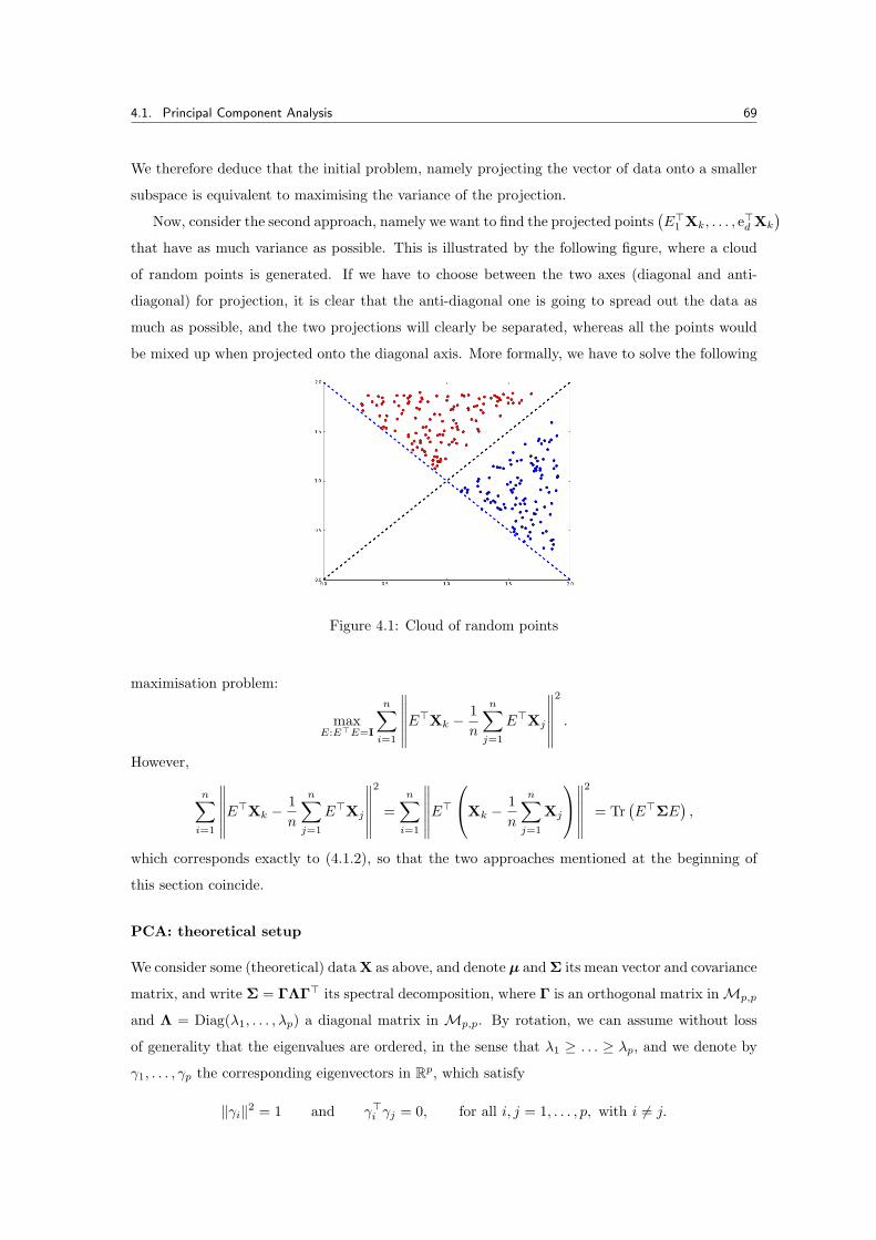
4.1. Principal Component Analysis 69
We therefore deduce that the initial problem, namely projecting the vector of data onto a smaller
subspace is equivalent to maximising the variance of the projection.
Now, consider the second approach, namely we want to find the projected points(E⊤
1 Xk, . . . , e⊤d Xk
)that have as much variance as possible. This is illustrated by the following figure, where a cloud
of random points is generated. If we have to choose between the two axes (diagonal and anti-
diagonal) for projection, it is clear that the anti-diagonal one is going to spread out the data as
much as possible, and the two projections will clearly be separated, whereas all the points would
be mixed up when projected onto the diagonal axis. More formally, we have to solve the following
Figure 4.1: Cloud of random points
maximisation problem:
maxE:E⊤E=I
n∑i=1
∥∥∥∥∥∥E⊤Xk − 1
n
n∑j=1
E⊤Xj
∥∥∥∥∥∥2
.
However,
n∑i=1
∥∥∥∥∥∥E⊤Xk − 1
n
n∑j=1
E⊤Xj
∥∥∥∥∥∥2
=n∑
i=1
∥∥∥∥∥∥E⊤
Xk − 1
n
n∑j=1
Xj
∥∥∥∥∥∥2
= Tr(E⊤ΣE
),
which corresponds exactly to (4.1.2), so that the two approaches mentioned at the beginning of
this section coincide.
PCA: theoretical setup
We consider some (theoretical) dataX as above, and denote µ andΣ its mean vector and covariance
matrix, and write Σ = ΓΛΓ⊤ its spectral decomposition, where Γ is an orthogonal matrix in Mp,p
and Λ = Diag(λ1, . . . , λp) a diagonal matrix in Mp,p. By rotation, we can assume without loss
of generality that the eigenvalues are ordered, in the sense that λ1 ≥ . . . ≥ λp, and we denote by
γ1, . . . , γp the corresponding eigenvectors in Rp, which satisfy
∥γi∥2 = 1 and γ⊤i γj = 0, for all i, j = 1, . . . , p, with i = j.
4.1. Principal Component Analysis 70
Definition 4.1.1. For any i = 1, . . . , p, the random variable ηi := γi(X − µ) is called the ith
principal component of the random vector X ∈ Rp.
The following properties are simple to prove:
Proposition 4.1.2. The random vector η is centered and its variance-covariance matrix satisfies
V[ηi] = λi and Cov[ηi,ηj ] = 0 for any i = j.
Example 4.1.3. Let X ∈ R2 be a random vector with
Σ =
1 ρ
ρ 1
,
for some ρ ∈ [0, 1]. It is easy to show that the eigenvalues are λ1 = 1 + ρ and λ2 = 1 − ρ, with
corresponding eigenvectors
γ1 =
1
1
and γ2 =
1
−1
.
Since ∥γ1∥2 = ∥γ2∥2, we need to normalise them, so that
γ1 =1√2
1
1
and γ2 =1√2
1
−1
.
and hence we can deduce the first two principal components
η1 =X1 +X2√
2and η2 =
X1 −X2√2
.
We can further compute the variances of the principal components:
V[η1] = V[X1 +X2√
2
]=
V[X1 +X2]
2=
V[X1] + V[X2] + 2Cov[X1, X2]
2= 1 + ρ = λ1,
V[η2] = V[X1 −X2√
2
]=
V[X1 −X2]
2=
V[X1] + V[X2]− 2Cov[X1, X2]
2= 1− ρ = λ2,
Theorem 4.1.4. Let X be a random vector in Rp with finite second moment, mean µ ∈ Rp and
variance-covariance matrix Σ. Then
argmaxa∈Rp:∥a∥=1
V(a⊤X) = argmaxa∈Rp:∥a∥=1
V(a⊤(X− µ)) = γ1.
Proof. From the spectral decomposition Σ = ΓΛΓ⊤, we can write
V(a⊤X) =
p∑i=1
λi(a⊤γi
) (γ⊤i a
)=:
p∑i=1
λic2i ,
where ci := a⊤γi is the projection of the vector a in the direction γi. Since the vectors γi form an
orthonormal basis, then∑p
i=1 c2i = ∥a∥2. Furthermore,
V(a⊤X
)=
p∑i=1
λic2i ≤ λ1
p∑i=1
c2i = λ1∥a∥2 = λ1.
4.1. Principal Component Analysis 71
With a = γ1, all the coefficients are therefore equal to zero except c1 = 1; the maximum is clearly
attained at this point since
V(γ⊤1 X
)= γ⊤1 V (X) γ1 = γ⊤1 Σγ1 = γ⊤1 (Σγ1) = γ⊤1 λ1γ1 = λ1∥γ1∥2 = λ1,
and the theorem follows.
In the previous theorem, we showed that the first principal direction is in fact given by the
eigenvector corresponding to the largest eigenvalue. It therefore sounds sensible to try and iterate
the procedure. In order to find the second component, the proof of the theorem holds with almost
no changes to prove that
γ2 = argmaxa∈A2
V(a⊤X) = argmaxa∈Rp:∥a∥=1
V(a⊤(X− µ)),
where
A2 := a ∈ Rp : ∥a∥ = 1, a ⊥ γ1 .
Indeed, repeating the arguments in the proof of the theorem, we can write, for any a ∈ A2,
V(a⊤X
)=
p∑i=2
λic2i ≤ λ2
p∑i=1
c2i = λ2∥a∥2 = λ2.
And we can iterate this procedure to any level up to p.
PCA: empirical analysis
We now consider a similar framework, but the the covariance matrix Σ replaced by the empirical
covariance matrix S. We can repeat the theoretical analysis, but now with empirical estimates.
Remark 4.1.5. Depending on the data, if several factors are expressed in different units, it might
be more appropriate to perform PCA with the correlation matrix rather than the covariance matrix,
as the former is unit-free.
Proposition 4.1.6 (Perron-Frobenius Theorem). Let A ∈ Mp,p a symmetric matrix with all
elements strictly positive. Then the coordinates of the first eigenvector all have the same sign.
Remark 4.1.7. The procedure to perform PCA is clear and the steps are as follows:
(i) Compute the covariance matrix Σ;
(ii) Apply the spectral decomposition theorem to Σ;
From a computational point of view, however, this may be too expensive. From the definition
of the covariance matrix, the cost of computing it is of order O(np2), and it can be shown that
the spectral decomposition has a cost of order O(p3). Assuming that n is of the same order as p
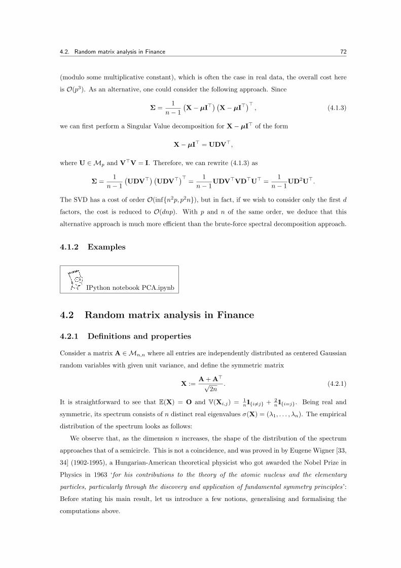
4.2. Random matrix analysis in Finance 72
(modulo some multiplicative constant), which is often the case in real data, the overall cost here
is O(p3). As an alternative, one could consider the following approach. Since
Σ =1
n− 1
(X− µI⊤
) (X− µI⊤
)⊤, (4.1.3)
we can first perform a Singular Value decomposition for X− µI⊤ of the form
X− µI⊤ = UDV⊤,
where U ∈ Mp and V⊤V = I. Therefore, we can rewrite (4.1.3) as
Σ =1
n− 1
(UDV⊤) (UDV⊤)⊤ =
1
n− 1UDV⊤VD⊤U⊤ =
1
n− 1UD2U⊤.
The SVD has a cost of order O(infn2p, p2n), but in fact, if we wish to consider only the first d
factors, the cost is reduced to O(dnp). With p and n of the same order, we deduce that this
alternative approach is much more efficient than the brute-force spectral decomposition approach.
4.1.2 Examples
IPython notebook PCA.ipynb
4.2 Random matrix analysis in Finance
4.2.1 Definitions and properties
Consider a matrix A ∈ Mn,n where all entries are independently distributed as centered Gaussian
random variables with given unit variance, and define the symmetric matrix
X :=A+A⊤√2n
. (4.2.1)
It is straightforward to see that E(X) = O and V(Xi,j) = 1n11i=j + 2
n11i=j. Being real and
symmetric, its spectrum consists of n distinct real eigenvalues σ(X) = (λ1, . . . , λn). The empirical
distribution of the spectrum looks as follows:
We observe that, as the dimension n increases, the shape of the distribution of the spectrum
approaches that of a semicircle. This is not a coincidence, and was proved in by Eugene Wigner [33,
34] (1902-1995), a Hungarian-American theoretical physicist who got awarded the Nobel Prize in
Physics in 1963 ‘for his contributions to the theory of the atomic nucleus and the elementary
particles, particularly through the discovery and application of fundamental symmetry principles’:
Before stating his main result, let us introduce a few notions, generalising and formalising the
computations above.
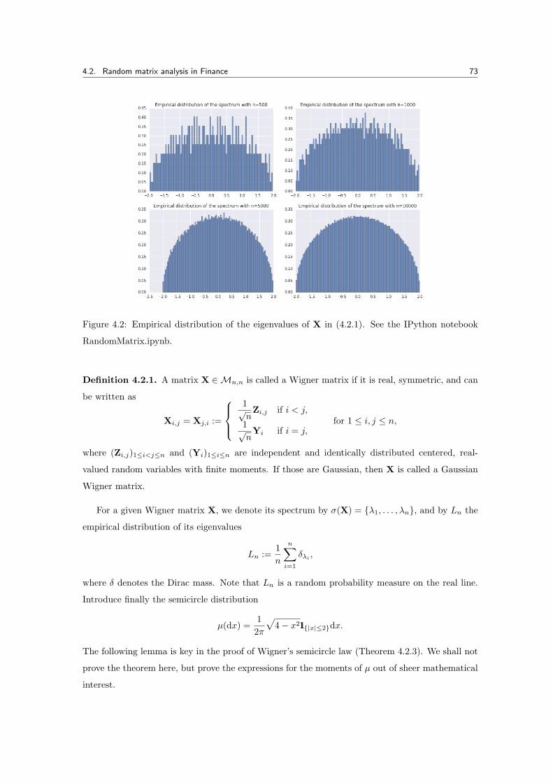
4.2. Random matrix analysis in Finance 73
Figure 4.2: Empirical distribution of the eigenvalues of X in (4.2.1). See the IPython notebook
RandomMatrix.ipynb.
Definition 4.2.1. A matrix X ∈ Mn,n is called a Wigner matrix if it is real, symmetric, and can
be written as
Xi,j = Xj,i :=
1√nZi,j if i < j,
1√nYi if i = j,
for 1 ≤ i, j ≤ n,
where (Zi,j)1≤i<j≤n and (Yi)1≤i≤n are independent and identically distributed centered, real-
valued random variables with finite moments. If those are Gaussian, then X is called a Gaussian
Wigner matrix.
For a given Wigner matrix X, we denote its spectrum by σ(X) = λ1, . . . , λn, and by Ln the
empirical distribution of its eigenvalues
Ln :=1
n
n∑i=1
δλi ,
where δ denotes the Dirac mass. Note that Ln is a random probability measure on the real line.
Introduce finally the semicircle distribution
µ(dx) =1
2π
√4− x211|x|≤2dx.
The following lemma is key in the proof of Wigner’s semicircle law (Theorem 4.2.3). We shall not
prove the theorem here, but prove the expressions for the moments of µ out of sheer mathematical
interest.
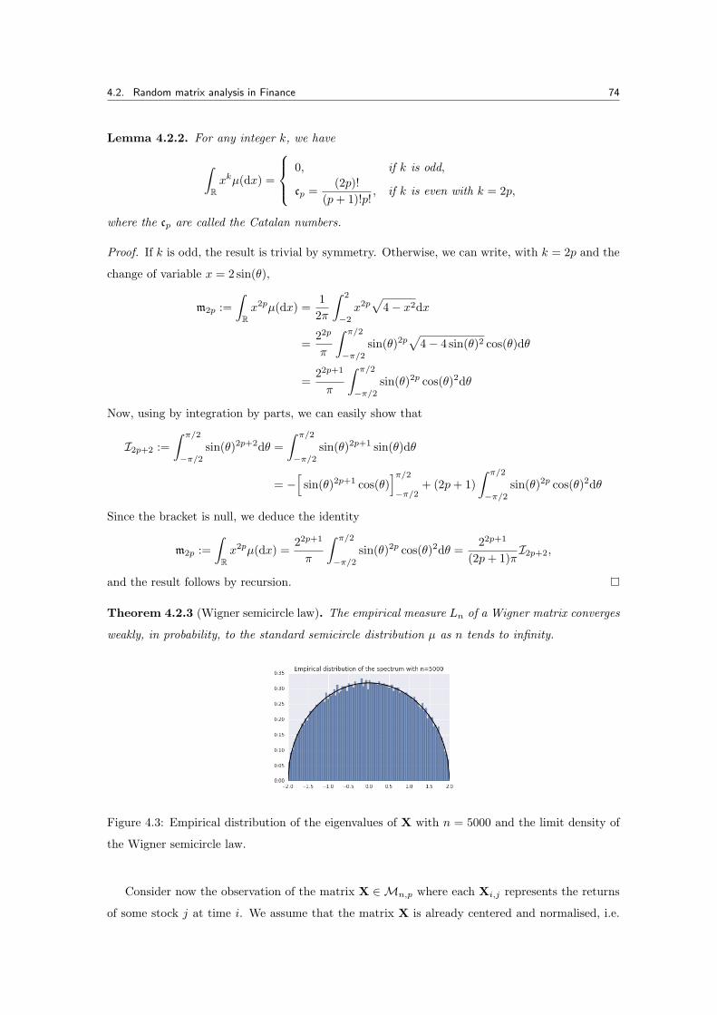
4.2. Random matrix analysis in Finance 74
Lemma 4.2.2. For any integer k, we have
∫Rxkµ(dx) =
0, if k is odd,
cp =(2p)!
(p+ 1)!p!, if k is even with k = 2p,
where the cp are called the Catalan numbers.
Proof. If k is odd, the result is trivial by symmetry. Otherwise, we can write, with k = 2p and the
change of variable x = 2 sin(θ),
m2p :=
∫Rx2pµ(dx) =
1
2π
∫ 2
−2
x2p√4− x2dx
=22p
π
∫ π/2
−π/2
sin(θ)2p√4− 4 sin(θ)2 cos(θ)dθ
=22p+1
π
∫ π/2
−π/2
sin(θ)2p cos(θ)2dθ
Now, using by integration by parts, we can easily show that
I2p+2 :=
∫ π/2
−π/2
sin(θ)2p+2dθ =
∫ π/2
−π/2
sin(θ)2p+1 sin(θ)dθ
= −[sin(θ)2p+1 cos(θ)
]π/2−π/2
+ (2p+ 1)
∫ π/2
−π/2
sin(θ)2p cos(θ)2dθ
Since the bracket is null, we deduce the identity
m2p :=
∫Rx2pµ(dx) =
22p+1
π
∫ π/2
−π/2
sin(θ)2p cos(θ)2dθ =22p+1
(2p+ 1)πI2p+2,
and the result follows by recursion.
Theorem 4.2.3 (Wigner semicircle law). The empirical measure Ln of a Wigner matrix converges
weakly, in probability, to the standard semicircle distribution µ as n tends to infinity.
Figure 4.3: Empirical distribution of the eigenvalues of X with n = 5000 and the limit density of
the Wigner semicircle law.
Consider now the observation of the matrix X ∈ Mn,p where each Xi,j represents the returns
of some stock j at time i. We assume that the matrix X is already centered and normalised, i.e.
4.2. Random matrix analysis in Finance 75
E(Xi,j) = 0 and V(Xi,j) = 1. The empirical covariance matrix Sn is the p × p symmetric matrix
defined as
Sn :=1
n
n∑i=1
XiX⊤i , (4.2.2)
where Xi ∈ Rp denotes the ith observation (or equivalently row i).
Definition 4.2.4. A matrix W ∈ Mp,p is said to have a Wishart distribution with scale matrix Σ
and n degrees of freedom, and we write W ∼Wp(n,Σ), if W = X⊤X with X ∼ Nn,p(0,Σ).
In the case where the scale matrix Σ is the identity matrix, W is called a white Wishart matrix.
A general Wp(n,Σ) Wishart distribution admits a density (available in closed form) only when
n ≥ p. We leave the following lemma regarding properties of Wishart distributions as an exercise:
Lemma 4.2.5. Let W1 ∼Wp(n1,Σ) and W2 ∼Wp(n2,Σ) be two independent Wishart matrices
and A ∈ Mp,q. Then A⊤W1A ∼Wq(n1,A⊤ΣA) and W1 +W2 ∈Wp(n1 + n2,Σ).
The following theorem explains why Wishart matrices are key for covariance estimation:
Theorem 4.2.6. The empirical covariance matrix in (4.2.2) satisfies Sn ∼ Wp(n − 1, n−1Σ),
where Σ is the true covariance matrix. Furthermore, the unbiased empirical covariance matrix
nn−1Sn is distributed as Wp(n− 1, 1
n−1Σ).
Remark 4.2.7. We shall not prove the theorem here, but it is easy to see that the empirical
covariance matrix Sn in (4.2.2) can be written as
Sn :=1
n
n∑i=1
XiX⊤i =
1
nX⊤HX,
where the so-called centering matrix H defined as H := I − n−11111⊤. It is easy to see that is a
projector, i.e. H2 = H and H⊤ = H.
The following result is classical and provides the asymptotic distribution of eigenvalues of
sample covariance matrices, when the sample size grows large, but for a fixed number of factors:
Theorem 4.2.8. Let Sn ∈ Mp,p be a sample covariance matrix drawn from Nn,p(µ,Σ) distribu-
tions, and denote by l1, . . . , lp its eigenvalues. Then, for any i = 1, . . . , p, as n tends to infinity,
√n (li − λi) converges in distribution to N (0, 2λ2i ),
where λ1, . . . , λp denote the eigenvalue of the true covariance matrix.
As mentioned before, however, p is in general of the same order as n, and the theorem does not
hold any longer. The following theorem is a key result in this framework, and was proved in [30].
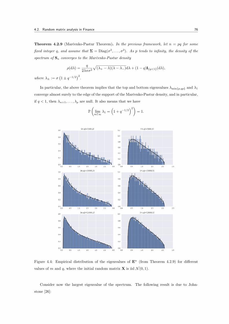
4.2. Random matrix analysis in Finance 76
Theorem 4.2.9 (Marcenko-Pastur Theorem). In the previous framework, let n = pq for some
fixed integer q, and assume that Σ = Diag(σ2, . . . , σ2). As p tends to infinity, the density of the
spectrum of Sn converges to the Marcenko-Pastur density
ρ(dλ) =q
2λπσ2
√(λ+ − λ)(λ− λ−)dλ+ (1− q)11q<1(dλ),
where λ± := σ(1± q−1/2
)2.
In particular, the above theorem implies that the top and bottom eigenvalues λminp,qp and λ1
converge almost surely to the edge of the support of the Marcenko-Pastur density, and in particular,
if q < 1, then λn+1, . . . , λp are null. It also means that we have
P(limm↑∞
λ1 =(1 + q−1/2
)2)= 1.
Figure 4.4: Empirical distribution of the eigenvalues of En (from Theorem 4.2.9) for different
values of m and q, where the initial random matrix X is iid N (0, 1).
Consider now the largest eigenvalue of the spectrum. The following result is due to John-
stone [26]:

4.2. Random matrix analysis in Finance 77
Proposition 4.2.10. Let W ∼Wp(n, I), and denote by λ1 its largest eigenvalue. Then (λ1−µ)/σ
converges in distribution to F1, where F1 is called the Tracy-Widom distribution of order one, and
µ :=(√n− 1 +
√m)2
and σ := µ((n− 1)−1/2 +m−1/2
)1/3.
4.2.2 Application: cleaning correlation matrices
IPython notebook Random Matrix.ipynb
Chapter 5
Regression Methods
5.1 Regression methods
5.1.1 Linear regression: the simple case
We start this chapter with the simple case of data (xi, yi)i=1,...,n, from which some dependency can
be observed. We would like to determine a relation of the form yi ≈ f(xi) for some function f :
R → R. A general formulation can be stated as
minf∈F
n∑i=1
Φ [yi − f(xi)] ,
for some given cost function Φ, where F is a class of functions of interest.
Simple linear regression
This is the simplest case, where we assume a dependence of the form
yi = f(xi) + εi, for i = 1, . . . , n
where f(x) ≡ α + βx is a linear function, and the sequence (εi)i=1,...,n are centered independent
random noises with constant variance σ2. We can rewrite this relation as Y = α11 + βX+ ε, with
X = (x1, . . . , xn)⊤ ∈ Rn, Y = (y1, . . . , yn)
⊤ ∈ Rn and ε = (ε1, . . . , εn)⊤ ∈ Rn.
Least-squares and properties
Since α and β are the only two parameters here, the infinite-dimensional minimisation problem
(over F) reduces to one over R2. In the least-square minimisation problem, we consider the
following loss / cost / error function:
L(α, β) := ∥Y − (α11 + βX)∥22 =n∑
i=1
(yi − α− βxi)2.
78
5.1. Regression methods 79
Definition 5.1.1. The least-square estimator (α, β) is the solution to the minimisation problem
(α, β) := argmin(α,β)
L(α, β). (5.1.1)
Proposition 5.1.2. The solution to (5.1.1) reads
α = y − βx and β =1
∥X− x11∥22
n∑i=1
(xi − x) yi.
Note that the computation of these estimators is purely deterministic and do not rely on the
iid assumption made about the errors.
Proof. Clearly, the function L is smooth, convex and hence admits a unique minimum, and
∇L(α, β) =
∂αL(α, β)∂βL(α, β)
= −2
n∑
i=1
(yi − α− βxi)
n∑i=1
xi (yi − α− βxi)
.
The first element can be written as
n∑i=1
(yi − α− βxi) = n (y − α− βx) ,
which is equal to zero if and only if α = y− βx. Regarding the gradient with respect to β, we can
write, plugging this optimal α,
n∑i=1
xi (yi − α− βxi) =n∑
i=1
xi [yi − (y − βx)− βxi] =n∑
i=1
xiyi − yn∑
i=1
xi + βxn∑
i=1
xi − βn∑
i=1
x2i ,
which is equal to zero if and only if
β =
∑ni=1 xi (yi − y)∑ni=1 xi (xi − x)
,
and the proposition follows.
Remark 5.1.3. Note that we can alternatively write the numerator and denominator in the
expression for β as follows:
n∑i=1
xi (yi − y) =n∑
i=1
xiyi − yn∑
i=1
xi =n∑
i=1
xiyi − ny x =n∑
i=1
xiyi − xn∑
i=1
yi =n∑
i=1
yi (xi − x) ,
and
∥X− x11∥22 =n∑
i=1
(xi − x)2=
n∑i=1
(x2i + x2 − 2xix
)=
n∑i=1
x2i + nx2 − 2xn∑
i=1
xi
=n∑
i=1
x2i − nx2 =n∑
i=1
xi (xi − x) . (5.1.2)
Let us prove some properties of these estimators:
5.1. Regression methods 80
Theorem 5.1.4. The LSE are unbiased and
V[β]=
σ2
∥X− x11∥22, V [α] =
σ2 ∥X∥22n ∥X− x11∥22
, Cov(α, β
)= − σ2x
∥X− x11∥22.
Proof. Let us first show the following alternative representation for β:
β = β +1
∥X− x11∥22
n∑i=1
(xi − x) εi. (5.1.3)
Combining the expression for β in Proposition 5.1.2 and the definition of the linear model Y =
α11 + βX+ ε, we can write
β =1
∥X− x11∥22
n∑i=1
(xi − x) yi =1
∥X− x11∥22
n∑i=1
(xi − x) [α+ βxi + εi]
=1
∥X− x11∥22
n∑i=1
(xi − x) [α+ βxi] +1
∥X− x11∥22
n∑i=1
(xi − x) εi.
Regarding the first term, we can write
1
∥X− x11∥22
n∑i=1
(xi − x) [α+ βxi] =1
∥X− x11∥22
[α
n∑i=1
(xi − x) + βn∑
i=1
xi (xi − x)
]= β,
sincen∑
i=1
(xi − x) = 0 and using the identity (5.1.2), so that (5.1.3) holds. Since the sequence
(ε1, . . . , εn) is iid, then clearly E[β] = β, and furthermore
E[α] = E[y − βx
]= y − βx = α.
It is also easy from (5.1.3) to show that
V[β]= V
[β +
1
∥X− x11∥22
n∑i=1
(xi − x) εi
]=
1
∥X− x11∥42
n∑i=1
(xi − x)2 V[εi]
=σ2
∥X− x11∥42
n∑i=1
(xi − x)2
=σ2
∥X− x11∥22,
using (5.1.2). Now, since α = y − βx by Proposition 5.1.2, we can write
V [α] = V[y − βx
]= V
[1
n
n∑i=1
yi − βx
]
= V
[1
n
n∑i=1
yi
]+ V
[βx]− 2x
n
n∑i=1
Cov(yi, β
)=σ2
n+ x2V
[β]− 2x
n
n∑i=1
Cov(yi, β
). (5.1.4)
5.1. Regression methods 81
Now, for any i = 1, . . . , n, we have, using (5.1.3),
Cov(yi, β
)= Cov
(yi, β +
1
∥X− x11∥22
n∑k=1
(xk − x) εk
)= Cov
(yi,
1
∥X− x11∥22
n∑k=1
(xk − x) εk
)
=1
∥X− x11∥22
n∑k=1
(xk − x)Cov (yi, εk) =σ2
∥X− x11∥22(xi − x) ,
since Cov (yi, εk) = 0 for all k = i and is equal to σ2 when k = i. Therefore Cov(y, β
)= 0.
Therefore, from (5.1.4), we obtain the desired variance of α. Finally,
Cov(α, β
)= Cov
(y − βx, β
)= Cov
(y, β
)− xV
[β]= −xV
[β]= − xσ2
∥X− x11∥22.
Theorem 5.1.5 (Gauss Markov). The LSE is optimal, in the sense that, among all possible
unbiased estimators linear in Y, it achieves minimal variance.
Proof. The estimator for β, which we can write as β =∑n
i=1 wiyi = w⊤Y, is clearly linear in Y.
Consider another unbiased estimator linear in Y: β := p⊤Y. We can then write
E[β]= p⊤E [α11 + βX+ ε] = αp⊤11 + βp⊤X
Since this new estimator is assumed unbiased and this relation holds for any β, we have αp⊤11 = 0
and p⊤X = 1. Now,
V[β]= V
[β − β + β
]= V
[β − β
]+ V
[β]+ 2Cov
(β − β, β
).
Now,
Cov(β − β, β
)= Cov
(β, β
)− V
[β]= 0,
so that we deduce V[β]≥ V
[β], and the theorem follows.
Note that in the results presented so far, the variances and covariance of the estimators depend
on the constant variance of the noise ε, which is actually unknown. We can however provide an
estimator for it. Define Y := α+ βX and ε := Y − Y.
Proposition 5.1.6. The statistics σ2 := 1n−2 ∥ε∥
22 is an unbiased estimator of σ2.
Proof. For any i = 1, . . . , n, since yi = α+ βxi + εi, then, summing over i yields y = α+ βx+ ε.
Therefore, for any i = 1, . . . , n, since y = α+ βx, we can write
εi := yi − yi = α+ βxi + εi −(α+ βxi
)= (y − βx− ε) + βxi + εi −
(y − βx
)− βxi
=(β − β
)(xi − x) + (εi − ε) .
5.1. Regression methods 82
Therefore, using (5.1.3) (in the second line),
∥ε∥22 =
n∑i=1
ε2i =(β − β
)2 n∑i=1
(xi − x)2+
n∑i=1
(εi − ε)2+ 2
(β − β
) n∑i=1
(xi − x) (εi − ε)
=(β − β
)2 n∑i=1
(xi − x)2+
n∑i=1
(εi − ε)2 − 2
(β − β
)2 n∑i=1
(xi − x)2
=n∑
i=1
(εi − ε)2 −
(β − β
)2∥X− x11∥22 ,
and hence
E[∥ε∥22
]= E
[n∑
i=1
(εi − ε)2 −
(β − β
)2∥X− x11∥22
]=
n∑i=1
E[(εi − ε)
2]− ∥X− x11∥22 V
[β]
= (n− 1)σ2 − σ2 = (n− 2)σ2.
Indeed,
n∑i=1
E[(εi − ε)
2]=
n∑i=1
E
ε2i + 1
n2
(n∑
i=1
εi
)2
− 2εn∑
i=1
εi
=
n∑i=1
[E[ε2i]+
1
n2E
[n∑
i=1
ε2i
]− 2εE
[n∑
i=1
εi
]]
=n∑
i=1
[σ2 +
σ2
n− 2
σ2
n
]= (n− 2)σ2.
The result then follows from Theorem 5.1.4.
One goal of regression methods is to predict the behaviour of variables. Suppose then that we
observe a new value, say xn+1, and we want to be able to predict the unknown value of yn+1. A
natural candidate is to consider yn+1 = α+ βxn+1. However, this yields the following error:
Proposition 5.1.7. The forecasting error εn+1 := yn+1 − yn+1 satisfies
E [εn+1] = 0 and V [εn+1] = σ2
(1 +
1
n+
(xn+1 − x)2
∥X− x11∥22
).
Proof. Since εn+1 is centered and the estimators α and β are unbiased, then
E [εn+1] = E[α− α] + E[β − β]xn+1 + E[εn+1] = 0.
Furthermore,
V [εn+1] = V[yn+1 − yn+1] = V[yn+1] + V[yn+1] = σ2 + V[yn+1].
5.1. Regression methods 83
The second term can be computed explicitly as
V[yn+1] = V[α+ βxn+1
]= V [α] + x2n+1V
[β]+ 2xn+1Cov
(α, β
)=
σ2
∥X− x11∥22
(1
n
n∑i=1
x2i + x2n+1 − 2xn+1x
)
=σ2
∥X− x11∥22
(1
n
n∑i=1
(xi − x)2+ x2 + x2n+1 − 2xn+1x
)
= σ2
(1
n+
(xn+1 − x)2
∥X− x11∥22
),
and the proposition follows.
A useful quantity when performing linear regression is the so-called coefficient of determina-
tion R2. Note first that, by Pythagoras’ Theorem,
TSS := ∥Y − y11∥22 =∥∥∥Y − y11
∥∥∥22+ ∥ε∥22 =: ESS + RSS,
so that the total sum of squares is equal to that explained by the model and the residual one.
Definition 5.1.8. The coefficient of determination R2 is defined as R2 :=ESS
TSS.
If R2 = 1, then the model fully explains the relationship, i.e. there is a perfectly linear relation
between X and Y. If R2 = 0, then ∥Y − y11∥ = 0, or yi = y for all i = 1, . . . , n, and the model is
completely inadequate.
Exercise 30. Show that R2 can also be understood as the square of the empirical correlation
coefficient between the two vectors X and Y, i.e. that
R2 =
(∑ni=1(xi − x)(yi − y)
∥X− x∥∥Y − y∥
)2
.
5.1.2 Study and estimation of the Gaussian linear regression model
We have so far assumed very little about the errors ε. In order to refine the analysis above, we
now assume that the sequence of errors (ε1, . . . , εn) is iid Gaussian with constant variance σ2.
The linear regression, given the vector X known (observed), becomes a simple assumption on the
Gaussian character of the output vector Y ∼ N (α+ βX, σ2). We can first compute the likelihood
of the sample as
Ln(α, β, σ2) =
(1
σ√2π
)n
exp
− 1
2σ2
n∑i=1
(yi − α− βxi)2
,
so that the log-likelihood to be minimised reads
ln(α, β, σ2) := − 1
nlogLn(α, β, σ
2) =n
2log(2πσ2
)+
∥Y − α11− βX∥222σ2
.
5.1. Regression methods 84
Minimising over α and β is straightforward and yields exactly the least-square estimates computed
above. Now,
∂σ2 ln(α, β, σ2) =
n
2σ2−
∥∥∥Y − α11− βX∥∥∥22
2σ4=
n
2σ2−
∥ε∥222σ4
,
which is equal to zero if and only if σ2 = σ2L := 1
n ∥ε∥22. It is easy to compute that
E[σ2L
]= E
[∥ε∥22n
]=n− 2
nσ2,
so that the maximum likelihood estimator of the variance is biased. Let us now look at the fine
properties of the estimators.
Theorem 5.1.9. Both α and β are Gaussian with means α and β and covariance matrix
Cov(α, β) =1
∥X− x11∥22
∥X∥22
n −x
−x 1
.
Furthermore,(n− 2)
σ2σ2 ∼ χ2
n−2, and β and σ2 are independent.
As before, one issue here is that the variance σ2 of the errors is actually unknown, and we can
replace it by its estimator, leading to more involved distributions for the above estimators. The
following proposition allows us to build confidence intervals for the estimators.
Proposition 5.1.10. Let tn−2 denote the Student law with n− 2 degrees of freedom, and define
σ2α :=
σ2
n∥X− x11∥22
n∑i=1
x2i and σ2β :=
σ2
∥X− x11∥22
the variance of the least square estimators. Then
• α− α
σα∼ tn−2 and
β − β
σβ∼ tn−2;
• The intervals[α− t
1−η/2n−2 σα, α+ t
1−η/2n−2 σα
]and
[β − t
1−η/2n−2 σβ , β + t
1−η/2n−2 σβ
]are the confidence intervals for α and β with level 1− η
2 .
Forecasting
Regarding forecasting, the general results above (without the Gaussian assumption for the errors)
still hold for the mean and the variance, so that Proposition 5.1.7 remains unchanged. However,
since σ2 is again unknown, we need to replace its value by the estimator σ2, and we obtain
Proposition 5.1.11.εn+1
σ
√1 + 1
n + (xn+1−x)2
∥X−x11∥22
∼ tn−2,
5.1. Regression methods 85
and the corresponding confidence interval for yn+1 reads[yn+1 − t
1−η/2n−2 σ
√1 +
1
n+
(xn+1 − x)2
∥X− x11∥22, yn+1 + t
1−η/2n−2 σ
√1 +
1
n+
(xn+1 − x)2
∥X− x11∥22
].
5.1.3 Linear regression: the multidimensional case
We now consider a multidimensional version of the previous linear regression, so that we are
interested in the following problem:
minf∈F
n∑i=1
Φ [yi − f(xi)] ,
for some given cost function Φ, where F is a class of functions of interest. The main difference here
is that, for each i = 1, . . . , n, xi is a vector in Rp, and the set F is composed of functions from Rp
to R. A multidimensional linear regression model is therefore a representation of the form
Y = Xβ + ε, (5.1.5)
where Y ∈ Rn is the response/measured/endogenous variable, X ∈ Mn,p(R) the exogenous or
explanatory variable, β ∈ Rp the vector of parameters to estimate, and ε ∈ Rn the noise vector
We shall always assume that the following conditions hold:
Assumption 5.1.12.
rank(X) = p and E[ε] = 0 and V[ε] = σ2In.
Exercise 31. Consider the one-dimensional model
yi = α+
p∑k=1
βkxki + εi,
for some integer p and all i = 1, . . . , n. Write this problem in a linear form.
Exercise 32. Consider now a function f of the form f(x) = a exp(γ⊤x
). Find a transform to
reduce the model to a linear form.
Least-square estimators
Definition 5.1.13. The least-square estimator is defined as
β = argminβ∈Rp
∥Y −Xβ∥22 .
We gather in the following proposition several results about β. Note that the optimality
statement is nothing else than a multi-dimensional version of the Gauss-Markov theorem (Theo-
rem 5.1.5).
5.1. Regression methods 86
Proposition 5.1.14. The optimal least-square estimator is β =(X⊤X
)−1X⊤Y and
E[β] = β and V[β] = σ2(X⊤X
)−1.
Note that the matrix X⊤X is invertible by Assumption 5.1.12.
Proof. The proof is a straightforward minimisation problem:
∇β ∥Y −Xβ∥22 = ∇β
(β⊤ (X⊤X
)β − 2Y⊤Xβ + ∥Y∥22
)= 2βX⊤X− 2Y⊤X.
Since the matrix X⊤X is invertible, the result for β follows directly. Now,
E[β] = E[(X⊤X
)−1X⊤Y
]=(X⊤X
)−1X⊤E [Y] =
(X⊤X
)−1X⊤E [Xβ + ε] = β.
Likewise,
V[β] = V[(X⊤X
)−1X⊤Y
]=(X⊤X
)−1X⊤V [Y]
(X⊤X
)−1X⊤⊤
=(X⊤X
)−1X⊤V [Y]X
(X⊤X
)−1⊤
= σ2(X⊤X
)−1X⊤X
(X⊤X
)−1⊤
,
since V[Y] = V[Xβ + ε] = V[ε] = σ2In, and the proposition follows.
Exactly like in the one-dimensional case, we can show that the least-square estimator is the
optimal one, in the following sense:
Theorem 5.1.15. Among all unbiased estimators of β linear in Y, the least-square estimator β
has minimal variance.
Proof. Let β be a linear estimator of β. Then
V[β]= V
[β − β + β
]= V
[β − β
]+ V
[β]+Cov
(β − β, β
)+Cov
(β, β − β
).
Since β is linear in Y, then we can write it β = AY for some matrix A ∈ Mp,n. Being unbiased,
it further satisfies
E[β]= β = AE [Xβ + ε] = AXβ +AE [ε] = AXβ,
so that AX = I. The covariance term then reads (recall Proposition 2.3.5 for such computations)
Cov(β − β, β
)= Cov
(AY − β, β
)= Cov
(AY, β
)− V
[β]
= Cov(AY,
(X⊤X
)−1X⊤Y
)− V
[β]
= AV [Y]X(X⊤X
)−1 − V[β]
= σ2AX(X⊤X
)−1 − V[β],
which is equal to zero since β is unbiased, and the theorem follows.
5.1. Regression methods 87
From a geometric point of view, least-square minimisation is equivalent to determining the
projection (in the Euclidean sense) of the random vectorY ontoMX, the subspace of Rn generated
by the column vectors of the matrix X. More specifically,
MX =
Xw =
p∑i=1
w1X1,w = (w1, . . . , wp) ∈ Rp
,
where we denote by Xi the i-th column of X. Since by assumption, X has rank p, then MX is
of dimension p. By Proposition 5.1.14, the projection therefore reads Y = Xβ =: PXY, where
PX := X(X⊤X
)−1X⊤ is called the orthogonal projection matrix onMX. (as a projection matrix,
check that P2X = PX). Now, the residuals of the least square estimation read
ε := Y − Y = Y −PXY = (In −PX)Y =: PX⊤Y = PX⊤ε.
The matrix PX⊥ is the orthogonal projection matrix onto MX⊥ . We can thus prove (exercise) the
following properties:
Proposition 5.1.16. The residuals are centered with V [ε] = σ2PX⊥ and
E[Y]= Xβ, V
[Y]= σ2PX, Cov
(ε, Y
)= 0.
Proposition 5.1.17. The estimator σ2 :=∥ε∥22n− p
is an unbiased estimator of the variance σ2.
Proof. First, note that
E[∥ε∥22
]= E
[Tr(∥ε∥22
)]= E
[Tr(ε⊤ε
)]= E
[Tr(ε ε⊤
)]= Tr
(E[ε ε⊤
])= Tr (V [ε]) = Tr
(σ2PX⊥
).
Finally, since
Tr (PX⊥) = Tr (In −PX) = Tr (In)− Tr (PX) = Tr (In)− Tr(X(X⊤X
)−1X⊥)= n− p,
the proposition follows.
This in turn, combined with Proposition 5.1.14, directly gives an estimator of the variance
of β. Regarding forecast, we again mimic the one-dimensional case. Consider a new observation
vector xn+1, with new response variable yn+1 = x⊤n+1β + εn+1, with E[εn+1] = 0, V[εn+1] = σ2
and Cov(εn+1, εi) = 0 for any i = 1, . . . , n. We define the new prevision as yn+1 := xn+1β, and
the prevision error εn+1 := yn+1 − yn+1.
Proposition 5.1.18. The following identities hold
E [εn+1] = 0 and V [εn+1] = σ2(1 + x⊤n+1
(X⊤X
)−1xn+1
).
Proof. Note first that
εn+1 := yn+1 − yn+1 = x⊤n+1β + εn+1 − x⊤n+1β = x⊤n+1
(β − β
)+ εn+1,
5.2. Departure from classical assumptions 88
so that, since εn+1 is centered and β is an unbiased estimator of β, we can write
E [εn+1] = E[x⊤n+1
(β − β
)+ εn+1
]= x⊤n+1
(β − E
[β])
= 0.
Now,
V [εn+1] = V[x⊤n+1
(β − β
)+ εn+1
]= V
[x⊤n+1
(β − β
)]+ V [εn+1] = x⊤n+1V
[β]xn+1 + σ2
since εn+1 is uncorrelated with (εi)i=1,...,n and β only depends on the latter sequence. The result
follows using Proposition 5.1.14.
5.2 Departure from classical assumptions
5.2.1 Overfitting and regularisation
When performing regression analysis, overfitting occurs when noise or errors are described, rather
than the actual relationships between the variables. This can essentially be due to two factors:
• the model may be too complicated (too many parameters compared to the number of obser-
vations). From Proposition 5.1.14, the matrix to invert is of size p×p, but has rank min(p, n).
Therefore is n < p, it is not invertible any longer;
• the data may contain some collinearity, when several explanatory variables are in fact highly
(linearly) dependent.
We shall see below how to regularise this issue, but let us discuss multicollinearity first.
Multicollinearity
Ridge regression
With the classical linear regression problem in mind (Definition 5.1.13), consider the loss function
L(β) := ∥Y −Xβ∥22 , (5.2.1)
which we aim to minimise. The ridge regression considers the minimisation, not of this loss
function, but of the alternative, L2-penalised version
LR(β) := ∥Y −Xβ∥22 + λ∥β∥22,
Following an analysis similar to the standard linear regression, we obtain that the optimal coefficient
is given by
βR =(X⊤X+ λI
)−1X⊤Y.
The advantage of this penalisation is clear: even if the original matrix X⊤X is not invertible, the
new version is, for λ > 0. Furthermore, as the parameter λ increases, the coefficients of β decrease,
making solutions with large coefficients less attractive.
5.2. Departure from classical assumptions 89
Meaning of the ridge regression
Consider the Singular Value Decomposition for the matrix X = UDV⊤. For the optimal linear
regression coefficient vector, we can then write
Xβ = X(X⊤X
)−1X⊤Y = UDV⊤
([UDV⊤]⊤ UDV⊤
)−1
[UDV⊤]⊤Y
= UDV⊤ (VD2V⊤)−1VDUY = UU⊤Y,
and in the case of ridge regression,
XβR =(X⊤X+ λI
)−1X⊤Y = UD
(D2 + λI
)−1DU⊤Y =
p∑j=1
ujd2j
d2j + λu⊤j Y,
where the uj represent the columns of the matrix U. The implication is that the ridge regression
applies more shrinkage when d2j is small; since d1, . . . , dp represent the eigenvalues of the ma-
trix X⊤X, ridge regression shrinks the coefficient β in the directions of small explained variances.
LASSO regression
This regression consists in penalising the loss function, not in the L2 sense as in the ridge regression,
but in the L1 sense, as
LL(β) := ∥Y −Xβ∥22 + λ∥β∥1.
Unfortunately, here there is no closed-form expression for the solution vector β, but this quadratic
programming problem is easy to solve numerically.
5.2.2 Underfitting
If overfitting is an issue, underfitting is also one, when explanatory variables are forgotten. Assume
that the true model is actually of the form
Y = Xβ + Zγ + ε,
where the error term ε satisfies the classical assumptions, and the columns of Z are linearly
independent of the columns of X. Then the estimator β (Proposition 5.1.14) satisfies
E[β]= E
[(X⊤X
)−1X⊤Y
]= E
[(X⊤X
)−1X⊤ (Xβ + Zγ)
]= E
[(X⊤X
)−1X⊤Xβ
]+ E
[(X⊤X
)−1X⊤Zγ
]= β +
(X⊤X
)−1X⊤Zγ =: β + Lγ,
where L is the matrix of regression coefficients omitted in the regression considering only the X
component. The estimator β is therefore biased. Note however that if the matrix Z is chosen
such that its columns are orthogonal to those of X, then X⊤Z = O and hence L = O, so that β
5.2. Departure from classical assumptions 90
becomes unbiased. Now, it is easy to see that the variance of the estimator remains unchanged
(see Proposition 5.1.14):
V[β]= V
[(X⊤X
)−1X⊤Y
]=(X⊤X
)−1X⊤V [Y]
((X⊤X
)−1X⊤)⊤
=(X⊤X
)−1X⊤V [Y]X
(X⊤X
)−1
=(X⊤X
)−1X⊤ [σ2In
]X(X⊤X
)−1
= σ2X⊤X.
However, concerning the estimator of the variance, similarly to Proposition 5.1.17, we can write
σ2 :=∥ε∥2
n− p=
(Y − Y
)⊤ (Y − Y
)n− p
=([In −PX]Y)
⊤([In −PX]Y)
n− p
=Y⊤ (In −PX)
⊤(In −PX)Y
n− p
=Y⊤ (In −PX)Y
n− p,
since the matrix In −PX is a projection matrix (onto MX⊥). Therefore,
(n− p)E[σ2]= E
[Y⊤ (In −PX)Y
]= Tr ((In −PX)V [Y]) + E[Y]⊤ (In −PX)E[Y]
= (n− p)σ2 + (Zγ)⊤ (In −PX)Zγ,
where we used the fact that the matrix In−PX annihilates all linear dependence on X and so does
not annihilate the Z part by assumption on the columns of Z. Therefore σ2 in general overestimates
the variance σ2. We also made use of the following simple result:
Lemma 5.2.1. Let Y be an Rn-valued random vector with second moment and A ∈ Mnn a
symmetric matrix. Then E[Y⊤AY
]= Tr (AV[Y]) + E[Y]⊤AE[Y].
Proof. Since Y⊤AY is of dimension one, it is equal to its trace, and hence
E[Y⊤AY
]= Tr
(E[Y⊤AY
])= E
[Tr(Y⊤AY
)]= E
[Tr(AYY⊤)]
= Tr(E[AYY⊤]) = Tr
(AE
[YY⊤]) = Tr
(AV[Y] + E[Y]E[Y]⊤
)= Tr (AV[Y]) + E[Y]⊤AE[Y].
5.2.3 Incorrect variance matrix
Suppose that, instead of σ2In, the variance of the error is in fact equal to σ2V, for some matrix
V ∈ Mnn. Then, it is straightforward to see that the estimator β remains unbiased. However,
V[β]= V
[(X⊤X
)−1X⊤Y
]= σ2
(X⊤X
)−1X⊤VX
(X⊤X
)−1,
5.2. Departure from classical assumptions 91
which is in general different from the variance of β under the classical assumption. Furthermore,
similar computations to above show that the estimator σ2 for the variance is in general biased, as
E[σ2]:=
E[Y⊤(In −PX)Y
]n− p
=σ2
n− pTr ((In −PX)V[Y]) = σ2Tr(V ).
5.2.4 Stochastic regressors
So far, one of the main assumptions of the model was that the regressor (or the vector of regressors)
was deterministic. This is not so realistic in practice, and we hence need to extend the results to
the case of random (or stochastic) regressors. We therefore rewrite the model (5.1.5) as
Y = Xβ + ε, (5.2.2)
together with Assumption 5.1.12. Regarding the variable X, we shall assume that the sequence
(εi, Xi)i=1,...,n is jointly iid. We now consider several dependence assumptions, each having par-
ticular consequences on the regression analysis:
• Independent X: this is the strongest assumption possible, meaning that the distributions
of X and ε are unrelated.
• Conditional zero mean: E[X|ε] = 0.
• Uncorrelated X: Cov(Xi, εi) = 0 for any i = 1, . . . , n.
• Corelated X: this is the most general case, where Cov(Xi, εi) = 0 for any i = 1, . . . , n.
It is easy to see that the above conditions are ordered from the strongest to the weakest, each
implying the weaker.
Remark 5.2.2. Suppose that we do not have accurate access to the data X, but only to a noisy
version X, say due to measurement errors (liquidity issues for some option prices, errors in the
discounting curve used...), of the form
X = X+ η,
where η represents the error. The linear regression model (5.2.2) therefore reads
Y = Xβ + ε =(X+ η
)β + ε = Xβ + (ηβ + ε) .
Now, even if the measurement error η is independent of the original error ε, the actual regressor X
will be correlated with the new error (ηβ + ε).
We now analyse the consequences of the randomness of the regressor on the linear regression.
Recall from Proposition 5.1.14 that the optimal least-square estimator is
β =(X⊤X
)−1X⊤Y
=(X⊤X
)−1X⊤ (Xβ + ε)
= β +(X⊤X
)−1X⊤ε
5.2. Departure from classical assumptions 92
For i = 1, . . . , p, we can then write
βi = βi +
p∑k=1
((X⊤X
)−1)ik
(X⊤ε
)k
= βi +
p∑k=1
((X⊤X
)−1)ik
n∑j=1
Xjkεk
= βi +
n∑j=1
[p∑
k=1
((X⊤X
)−1)ikXjk
]εj =: βi +
n∑j=1
wiεj
If εj is uncorrelated with Xk for j = k, it might not be so, in general, with the non-linear (in X)
term w, so that, in general, we will have
E[β]= β + E
[(X⊤X
)−1X⊤ε
]= β.

Appendix A
Useful tools in probability theory
and analysis
A.1 Useful tools in linear algebra
Let n ∈ N and consider a matrix A = (aij)1≤i,j≤n ∈ Mn(R).
Definition A.1.1. The matrix A is said to be positive definite (respectively positive semi-definite)
if xtAx > 0 (resp ≥ 0) for all non null vector x ∈ Rn.
For a matrix A ∈ Mn(R), we define its principal minors as
∆1 := a11, ∆2 := det
a11 a12
a21 a22
, . . . , ∆n := det(A).
Proposition A.1.2. The following statements are equivalent:
(i) A is positive definite;
(ii) all the eigenvalues of A are positive;
(iii) all leading principal minors of A are positive.
Exercise 33. Let S ⊂ Rn be a convex and open set. Let f be a continuously differentiable
function on S. Recall that the function f is convex in S if for any two points x and y in S, the
following inequality holds:
f (αx + (1− α)y) ≤ αf(x) + (1− α)f(y), for any α ∈ [0, 1].
Show the following:
(i) f is convex if and only if f(y) ≥ f(x) +∇f(x)T · (y − x) for all (x, y) ∈ S × S;
93

A.1. Useful tools in linear algebra 94
(ii) if f is twice continuously differentiable on S, then f is convex if and only if the matrix ∇2f(x)
is positive semi-definite for all x ∈ S.
Definition A.1.3. The spectral radius ρ of a matrix A ∈ Mn(R) is defined by ρ(A) := max1≤i≤n λi,
where λ1, . . . , λn are the eigenvalues of A.
Bibliography
[1] M. Abramowitz and I. Stegun. Handbook of Mathematical Functions with Formulas, Graphs,
and Mathematical Tables. New York: Dover Publications, 1972.
[2] L.B.G. Andersen, P. Jackel and C. Kahl. Simulation of Square-Root Processes. Encyclopedia
of Quantitative Finance, 2010.
[3] K.E. Atkinson. An introduction to numerical analysis, Second Edition. Wiley, 1989.
[4] D. H. Bailey and P. N. Swarztrauber. The fractional Fourier transform and applications.
SIAM Review,33: 389-404, 1991.
[5] A.C. Berry. The Accuracy of the Gaussian Approximation to the Sum of Independent Vari-
ates. Transactions of the American Mathematical Society, 49 (1): 122-136, 1941.
[6] P. Billingsley. Convergence of probability measures (2nd ed.). John Wiley & Sons, 1999.
[7] F. Black and M. Scholes. The Pricing of Options and Corporate Liabilities. Journal of Po-
litical Economy, 81 (3): 637-654, 1973.
[8] P. Boyle. Option Valuation Using a Three-Jump Process. International Options Journal 3,
7-12, 1986.
[9] P. Carr, H. Geman, D. Madan and M. Yor. Stochastic volatility for Levy processes. Mathe-
matical Finance, 13(3): 345-382, 2003.
[10] P. Carr and D. Madan. Option valuation using the fast Fourier transform. Journal of Com-
putational Finance, 2 (4): 61-73, 1999.
[11] P. Carr and D. Madan. Saddlepoint Methods for Option Pricing. Journal of Computational
Finance, 13 (1): 4961, 2009.
[12] A.L. Cauchy. Cours d’analyse de l’Ecole Royale Polytechnique. Imprimerie royale, 1821.
Reissued by Cambridge University Press, 2009.
95
Bibliography 96
[13] R. Cont and E. Voltchkova. A finite difference scheme for option pricing in jump diffusion and
exponential Levy models. SIAM Journal On Numerical Analysis, 43(4): 1596-1626, 2005.
[14] J.W. Cooley and J.W. Tukey. An algorithm for the machine calculation of complex Fourier
series. Mathematics of Computation, 19: 297-301, 1965.
[15] M. Cooney. Report on the accuracy and efficiency of the fitted methods for solving the Black-
Scholes equation for European and American options. Working report, Datasim Education
Ltd, Dublin, 2000.
[16] R. Courant, K. Friedrichs and H. Lewy. Uber die partiellen Differenzengleichungen der math-
ematischen Physik. Mathematische Annalen, 100 (1): 32-74, 1928.
[17] J.C. Cox, J.E. Ingersoll and S.A. Ross. A Theory of the Term Structure of Interest Rates.
Econometrica, 53: 385-407.
[18] J.C. Cox, S.A. Ross and M. Rubinstein. Option Pricing: A Simplified Approach. Journal of
Financial Economics, 7: 229-263, 1979.
[19] J.Crank and P. Nicolson. A Practical Method for Numerical Evaluation of Solutions of Partial
Differential Equations of Heat Conduction Type. Proceedings of the Cambridge Philosophical
Society 43: 50-67, 1947.
[20] F. Delbaen and W. Schachermayer. A general version of the fundamental theorem of asset
pricing. Math Ann, 300(1): 463-520, 1994.
[21] F. Delbaen and W. Schachermayer. The Mathematics of arbitrage. Springer, 2008.
[22] J. Douglas and H.H. Rachford. On the numerical solution of heat conduction problems in
two and three space variables. Transactions of the AMS, 82:421-439, 1956.
[23] D. Duffie, D. Filipovic, and W. Schachermayer. Affine processes and applications in finance.
The Annals of Applied Probability, 13(3): 984-1053, 2003.
[24] C.-G. Esseen. On the Liapunoff limit of error in the theory of probability. Arkiv f’ur Matem-
atik, Astronomi och Fysik, A28: 1-19, 1942.
[25] B. Flannery, W.H. Press, S. Teukolsky and W. Vetterling. Numerical Recipes. Cambridge
University Press, Third Edition, 2007.
[26] I.M. Johnstone. On the distribution of the largest eigenvalue in principal component analysis.
Annals of Statistics, 29(2): 295-327, 2001.
[27] S. Kullback and R.A. Leibler. On information and sufficiency. The Annals of Mathematical
Statistics, 22(1), 79-86, 1951.

Bibliography 97
[28] J. Lintner. The valuation of risk assets and the selection of risky investments in stock port-
folios and capital budgets. Review of Economics and Statistics, 47(1): 13-37, 1965.
[29] R. Lugannani and S.O. Rice. Saddlepoint approximations for the distribution of the sum of
independent random variables. Advances in Applied Probability, 12: 475-490, 1980.
[30] V.A. Marchenko and L.A. Pastur. Distribution of eigenvalues for some sets of random ma-
trices. Mat. Sb. N.S. (in Russian). 72 (114:4): 507-536, 1967.
[31] K. Pearson. On lines and planes of closest
to systems of points in space. Philosophical Magazine, Series 6, 2(11):559-572, 1901.
[32] W.F. Sharpe. Capital asset prices: A theory of market equilibrium under conditions of risk.
Journal of Finance, 19 (3): 425-442, 1964.
[33] E. Wigner. Characteristic vectors of bordered matrices with infinite dimensions. Annals of
Mathematics, 62: 548-564, 1955.
[34] E. Wigner. On the distribution of the roots of certain symmetric matrices. Annals of Math-
ematics, 67: 325-328, 1958.
[35] A.T.A Wood, J.G. Booth and R.W. Butler. Saddlepoint approximations with nonnormal
limit distributions. Journal of the American Statistical Association, 88: 680-686, 1993.