Statistical Analysis of a Round-Robin Measurement Survey ... · RTI International, Research Triangle Park, NC 27709 R. Willigan United Technologies Research Center, ... resurgence

Volume 114, Number 1, January-February 2009Journal of Research of the National Institute of Standards and Technology

37

[J. Res. Natl. Inst. Stand. Technol. 114, 37-55 (2009)]

Statistical Analysis of a Round-RobinMeasurement Survey of Two Candidate

Materials for a Seebeck CoefficientStandard Reference Material

Volume 114 Number 1 January-February 2009

Z. Q. J. Lu, N. D. Lowhorn,W. Wong-Ng, W. Zhang, E. L.Thomas, M. Otani, M. L. Green

National Institute of Standardsand Technology,Gaithersburg, MD 20899T. N. Tran

Naval Surface Warfare Center,West Bethesda, MD 20817C. Caylor

RTI International, ResearchTriangle Park, NC 27709N. R. Dilley

Quantum Design,San Diego, CA 92121A. Downey

Armor Holdings,Sterling Heights, MI 48310andMichigan State University,East Lansing, MI 48824B. Edwards

Clemson University,Clemson, SC 29634N. Elsner, S. Ghamaty

Hi-Z Technology, Inc.,San Diego, CA 92126

T. Hogan

Armor Holdings,Sterling Heights, MI 48310

Q. Jie, Q. Li

Brookhaven National Laboratory,Upton, NY 11973

J. Martin, G. Nolas

University of South Florida,Tampa, FL 33620H. Obara

Advanced Institute of Scienceand Technology,Ibaraki, JapanJ. Sharp

Marlow Industries, Inc.,Dallas, TX 75238R. Venkatasubramanian

RTI International, ResearchTriangle Park, NC 27709R. Willigan

United Technologies ResearchCenter,East Hartford, CT 06108J. Yang

General Motors R&D Center,Warren, MI 48090

and

T. Tritt

Clemson University,Clemson, SC [email protected]@[email protected]@[email protected][email protected]@[email protected]@[email protected]@[email protected]@[email protected]@[email protected]

[email protected]@[email protected]@[email protected]@[email protected]@[email protected]

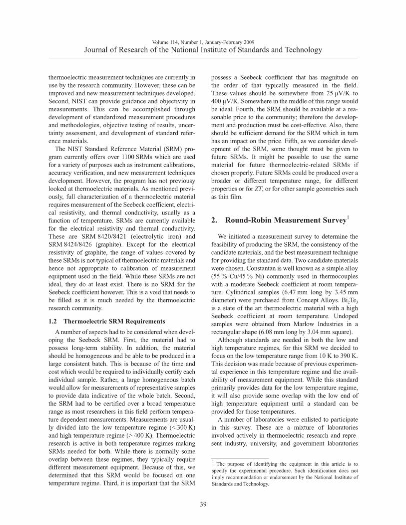
In an effort to develop a StandardReference Material (SRM™) for Seebeckcoefficient, we have conducted around-robin measurement survey of twocandidate materials—undoped Bi2Te3 andConstantan (55 % Cu and 45 % Ni alloy).Measurements were performed in tworounds by twelve laboratories involved inactive thermoelectric research using anumber of different commercial andcustom-built measurement systems andtechniques. In this paper we report thedetailed statistical analyses on theinterlaboratory measurement results andthe statistical methodology for analysis ofirregularly sampled measurement curves inthe interlaboratory study setting. Based onthese results, we have selected Bi2Te3 asthe prototype standard material. Onceavailable, this SRM will be useful forfuture interlaboratory data comparison andinstrument calibrations.

Key words: bismuth telluride; consensusmean curve; Constantan; functional dataanalysis; Ridge regression modeling;round-robin; Seebeck coefficient; StandardReference Material; thermoelectric.

Accepted: November 28, 2008

Available online: http://www.nist.gov/jres

1. Introduction

Thermoelectricity is the study of the direct conver-sion between thermal and electrical energy through theSeebeck and Peltier effects. In the Seebeck effect, apotential difference arises when a junction between twodissimilar conductors is heated or cooled [1].theSeebeck effect can be used for power generation appli-cations. Conversely, when a current passes through thejunction between two dissimilar conductors, heat isabsorbed or expelled at the junction depending on thedirection of current flow. This is known as the Peltiereffect and can be used for electronic refrigeration [2].

Seebeck coefficient (α) is defined as the voltage (V)generated per degree of temperature difference betweentwo points (α = ΔV/ΔT). The Seebeck effect has beenused by NASA to supply power for deep space probesin its radioisotope thermoelectric generators (RTGs)and is of current interest to automobile manufacturersto supply additional power through waste heat recov-ery. RTGs have provided long term reliability withsome deep space probes approaching three decades ofconstant operation. The Peltier effect can be used forelectronics spot cooling of computer processors and haswidely been used to thermally manage optoelectronicdevices such as communication lasers and infra-reddetectors. A more common use is in portableheaters/coolers that can be purchased inexpensively atmany local stores. While wider use of thermoelectricsin more mainstream applications holds great promisebecause of their high reliability and environmentalfriendliness, the low efficiency with which they operatehas restricted their usage. Recently, there has been aresurgence of activity in this field to find novel materi-als that can operate with higher efficiency to providealternative power generation options and competitionwith conventional refrigeration technology.

The efficiency of a thermoelectric material is direct-ly related to the thermoelectric figure of merit ZT givenby α2σT/κ where σ is the electrical conductivity, κ isthe thermal conductivity, and T is the absolute temper-ature. The current state of the art thermoelectricmaterials from the (Bi1–XSbX) 2 (Te1–YSeY)3, Bi1–XSbX,Si1–XGeX, and PbTe systems all have maximum ZTvalues of around 1 at their respective optimum temper-atures. Although this value has been the maximum forover 40 years, there exists no theoretical reason for thisto be absolute limit [3]. Several recent reports haveindicated that much higher ZTs are possible both in thinfilm superlattices [4] and in bulk materials [5]. A ZT of3 to 4 would indicate an efficiency great enough toallow direct competition with conventional refrigera-

tion devices [6]. While full evaluation of a materialrequires measurement of the electrical resistivity orconductivity, Seebeck coefficient and thermal conduc-tivity, measurement of just the Seebeck coefficient canfilter out those materials which do not have the desiredthermoelectric properties. There exists a minimumSeebeck coefficient that must be achieved to give adesired ZT. If this Seebeck coefficient is not achieved,the material does not warrant further study as the otherproperties can not overcome a deficiency in theSeebeck coefficient. For ZT = 1, the Seebeck coeffi-cient must be ≥ 157 μV/K; for ZT = 2, the Seebeckcoefficient must be ≥ 222 μV/K. The derivation of thisminimum Seebeck coefficient assumes the ideal case inwhich the lattice thermal conductivity is zero. Becausethe lattice thermal conductivity will not be zero in anyreal system, the actual Seebeck coefficient must besomewhat higher [7].

One of the needs that persist in this research field isthat of a Seebeck coefficient standard reference materi-al (SRM) to help ensure reliable measurements andcharacterization. Researchers building measurementequipment need to be able to calibrate their systems toknown values in order to ensure consistency withdifferent equipment in other laboratories. Numerouslaboratories perform thermoelectric materials charac-terization through measurement of the electrical resis-tivity or conductivity, thermal conductivity, andSeebeck coefficient. These required measurements aredemanding, especially the thermal conductivity meas-urements; however, one of the most important initialmeasurements is that of the Seebeck coefficient due tothe minimum requirements. Standard reference materi-als exist for thermal conductivity and electrical conduc-tivity, and there are reliable low Seebeck coefficientmaterials such as Pb or Pt; however, there is no highSeebeck coefficient SRM [8].

1.1 National Institute of Standards and Technology(NIST) and Thermoelectrics

Research efforts at NIST are guided by the NISTmission and vision statements. The NIST mission is“to promote U.S. innovation and industrial competitive-ness by advancing measurement science, standards, andtechnology in ways that enhance economic security andimprove quality of life.” The NIST vision is “to be theglobal leader in measurement and enabling technology,delivering outstanding value to the nation.”

With respect to the thermoelectric research commu-nity, the NIST mission and vision can be applied in twoareas. First, NIST can help develop the metrology ofthermoelectric measurements. A number of excellent


38

thermoelectric measurement techniques are currently inuse by the research community. However, these can beimproved and new measurement techniques developed.Second, NIST can provide guidance and objectivity inmeasurements. This can be accomplished throughdevelopment of standardized measurement proceduresand methodologies, objective testing of results, uncer-tainty assessment, and development of standard refer-ence materials.

The NIST Standard Reference Material (SRM) pro-gram currently offers over 1100 SRMs which are usedfor a variety of purposes such as instrument calibrations,accuracy verification, and new measurement techniquesdevelopment. However, the program has not previousylooked at thermoelectric materials. As mentioned previ-ously, full characterization of a thermoelectric materialrequires measurement of the Seebeck coefficient, electri-cal resistivity, and thermal conductivity, usually as afunction of temperature. SRMs are currently availablefor the electrical resistivity and thermal conductivity.These are SRM 8420/8421 (electrolytic iron) andSRM 8424/8426 (graphite). Except for the electricalresistivity of graphite, the range of values covered bythese SRMs is not typical of thermoelectric materials andhence not appropriate to calibration of measurementequipment used in the field. While these SRMs are notideal, they do at least exist. There is no SRM for theSeebeck coefficient however. This is a void that needs tobe filled as it is much needed by the thermoelectricresearch community.

1.2 Thermoelectric SRM RequirementsA number of aspects had to be considered when devel-

oping the Seebeck SRM. First, the material had topossess long-term stability. In addition, the materialshould be homogeneous and be able to be produced in alarge consistent batch. This is because of the time andcost which would be required to individually certify eachindividual sample. Rather, a large homogeneous batchwould allow for measurements of representative samplesto provide data indicative of the whole batch. Second,the SRM had to be certified over a broad temperaturerange as most researchers in this field perform tempera-ture dependent measurements. Measurements are usual-ly divided into the low temperature regime (< 300 K)and high temperature regime (> 400 K). Thermoelectricresearch is active in both temperature regimes makingSRMs needed for both. While there is normally someoverlap between these regimes, they typically requiredifferent measurement equipment. Because of this, wedetermined that this SRM would be focused on onetemperature regime. Third, it is important that the SRM

possess a Seebeck coefficient that has magnitude onthe order of that typically measured in the field.These values should be somewhere from 25 μV/K to400 μV/K. Somewhere in the middle of this range wouldbe ideal. Fourth, the SRM should be available at a rea-sonable price to the community; therefore the develop-ment and production must be cost-effective. Also, thereshould be sufficient demand for the SRM which in turnhas an impact on the price. Fifth, as we consider devel-opment of the SRM, some thought must be given tofuture SRMs. It might be possible to use the samematerial for future thermoelectric-related SRMs ifchosen properly. Future SRMs could be produced over abroader or different temperature range, for differentproperties or for ZT, or for other sample geometries suchas thin film.

2. Round-Robin Measurement Survey1

We initiated a measurement survey to determine thefeasibility of producing the SRM, the consistency of thecandidate materials, and the best measurement techniquefor providing the standard data. Two candidate materialswere chosen. Constantan is well known as a simple alloy(55 % Cu/45 % Ni) commonly used in thermocoupleswith a moderate Seebeck coefficient at room tempera-ture. Cylindrical samples (6.47 mm long by 3.45 mmdiameter) were purchased from Concept Alloys. Bi2Te3

is a state of the art thermoelectric material with a highSeebeck coefficient at room temperature. Undopedsamples were obtained from Marlow Industries in arectangular shape (6.08 mm long by 3.04 mm square).

Although standards are needed in both the low andhigh temperature regimes, for this SRM we decided tofocus on the low temperature range from 10 K to 390 K.This decision was made because of previous experimen-tal experience in this temperature regime and the avail-ability of measurement equipment. While this standardprimarily provides data for the low temperature regime,it will also provide some overlap with the low end ofhigh temperature equipment until a standard can beprovided for those temperatures.

A number of laboratories were enlisted to participatein this survey. These are a mixture of laboratoriesinvolved actively in thermoelectric research and repre-sent industry, university, and government laboratories


39

1 The purpose of identifying the equipment in this article is tospecify the experimental procedure. Such identification does notimply recommendation or endorsement by the National Institute ofStandards and Technology.

both domestic and international. These participants andthe primary researcher from each are listed in Table 1.

2.1 Measurement EquipmentA number of measurement systems were used in this

study including both commercial and custom-builtsystems. The measurements were carried out withseveral different measurement techniques (some systemswere capable of multiple techniques).

2.1.1 Commercial SystemsThe Quantum Design Physical Property Measurement

System (PPMS) with Thermal Transport Option (TTO)is a versatile system which can measure the Seebeckcoefficient from 2 K to 400 K in several different modes,each of which was used in this study. Samples can bemounted in either a 2 or 4-probe configuration, andmeasurements can be performed with a stable sampletemperature or dynamic sample temperature (usually≤ 0.5 K/min). The dynamic measurements continuouslymonitor the ΔT and ΔV along the sample while supply-ing a heat pulse to one end and slowly varying thesample temperature. This approach gives the ability tomeasure the Seebeck coefficient as a function of temper-ature without having to wait for stability and datacollection at each temperature. The steady-state valuesfor ΔT and ΔV are found by extrapolating the data froma relatively short heat pulse. This system prefers asample geometry such that the thermal conductance at300 K is between 1-5 mW/K for 2-probe measurements.

Bar- or disc-shaped, gold-plated, copper contact leadswere used and attached to the sample with either solderor silver epoxy (EpoTek H20E). The versatility of thissystem also allows for integrating 3rd party electronicsand/or software to perform custom measurements. Onelaboratory provided data using this system with aKeithley nanovoltmeter to measure the Seebeck voltagewhile performing a direct steady-state DC measurement.

The ULVAC RIKO ZEM-2 system performs a steady-state sweep technique and operates in two modes tocover different temperature regimes. The cryostat modeallows measurements from 193 K - 373 K while thefurnace mode allows measurements from room tempera-ture to 1273 K. This system prefers samples 13 mm orlonger while at least 8 mm of length is recommended bythe vendor. Using samples shorter than this length intro-duces error due to smaller probe spacing and temperaturedifference. The samples in this study were only 6 mmlong and required extenders to span the length not cov-ered by the sample. A 4-probe measurement geometrywas used with chromel or platinum lead wires attachedto the ends of the samples and Type K (Type M8 and L)or R(Type M10) thermocouple probes attached to thesides. In this steady-state sweep technique, the samplewas held at a constant temperature while one end ofthe sample was heated to produce a constant tempera-ture gradient. The temperature and voltage differencebetween the thermocouple probes was measured. Thenext temperature diference value was attained, andmeasurements were repeated. After all temperaturedifference setpoints at a particular sample temperaturewere covered, the slope of the voltage difference (ΔV) vstemperature difference (ΔT) gave the Seebeck coefficientat that sample temperature. After this, the sample tem-perature was changed, and the measurement wasrepeated.

2.1.2 Custom SystemsThree laboratories used systems which allowed for

measurements over a broad temperature range coveringmuch of the target range for this study. Each of theseemployed different measurement techniques and samplemounting, however.

The first system used a steady-state sweep techniquein which the sample was held at a constant temperatureand the ΔT was slowly ramped through a range of valueswhile monitoring the ΔV. The data was linearly fit, andthe slope yielded the Seebeck coefficient. A small resis-tor was epoxied to the top of the sample, and the oppo-site end was soldered to a heat sink. Two differentialthermocouple contacts were made to the sides of the


40

Table 1. Round-robin measurement survey participants

Primary Researcher Laboratory

Neil Dilley Quantum DesignNorbert Elsner Hi-Z TechnologyTim Hogan Michigan State UniversityQiang Li Brookhaven National LaboratoryNathan Lowhorn National Institute of Standards

and TechnologyGeorge Nolas University of South FloridaHaruhiko Obara National Institute of Advanced

Industrial Science andTechnology—Japan

Jeffrey Sharp Marlow IndustriesTerry Tritt Clemson UniversityRama Venkatasubramanian RTI InternationalRhonda Willigan United TechnologiesJihui Yang General Motors

sample for measuring the ΔT, and a thermocoupleepoxied between the differential thermocouple contactsmeasured the average sample temperature.

The second system used a 4-probe configuration inwhich current was pulsed through a small platinumheater resistor on one end of the sample to generate theΔT. The other end of the sample was attached to theprobe using solder or silver paste. Silver paste was usedto attach type-E thermocouples to the sample tomeasure the ΔT.

The third system used a pseudo-steady-state tech-nique in which a constant ΔT was applied along thesample, and measurements of the ΔV were made as thesample temperature was slowly changed (≤ 1 K/min).A smaller ΔT calculated from a percentage of thesample temperature was used as the temperature wasdecreased. Samples were soldered between 2 copperblocks which acted as voltage probes for measuring theΔV. The junctions of a differential thermocouple wereembedded in the copper blocks to measure the ΔT.

The other systems only measured at or near roomtemperature. Three of these used a simple ΔT sweeptechnique but had sight sample mounting variations. Inthe first technique, copper end caps were soldered tothe ends of the sample, and each cap included a copperwire and a 3 mil Type T thermocouple. One end of thesystem was thermally sunk to a thermoelectric coolerto provide basic sample temperature control. In thesecond technique, samples were mounted between 2copper blocks and partially exposed above the blocks.To the exposed parts, voltage and thermocouple probeswere attached. Cartridge heaters were embedded ineach block to control the ΔT. Two measurements wereperformed at each temperature with reversed thermo-couples to account for thermocouple variations. Thesample was slowly swept through a range of ΔT valueswhich centered on the temperature being measured. Inthe third technique, samples were clamped betweentwo clean copper blocks each embedded with a heaterand thermocouple. The blocks were held at differenttemperatures and ramped slowly through different ΔTvalues while the ΔV was recorded. A linear fit to thedata gave the Seebeck coefficient.

One of the other systems used a basic single pointmeasurement. Samples were mounted between 2 nickel-plated copper blocks held at different temperatures toproduce a ΔT along the sample. The ΔV between the2 blocks was measured and divided by the ΔT to givethe Seebeck coefficient.

The last system used a Harman technique in which aΔT was produced along the sample by means of thePeltier effect when a current was passed through thesample. After stabilization, the current was switchedoff; and the ohmic and Seebeck voltages were separat-ed from the total voltage. Measurements were repeatedusing opposite current sense to account for thermo-couple differences and voltmeter offsets.

2.2 Round-Robin ProcedureThe measurements were conducted in two rounds to

allow each sample to be measured by 2 differentlaboratories and provide a good amount of comparativedata while working within the time constraints of theproject and the participants. The ideal situation wouldbe where each sample is measured by all laboratories.However, due to the nature of these measurements, thiswould require an extreme time commitment by eachlaboratory and would greatly lengthen the SRM projectas a whole. This was not practical. The procedure weused allowed each measurement technique to be per-formed on 2 different samples and for each sample tobe measured by 2 different laboratories. Also, multiplesamples were measured at NIST using one technique toprovide additional sample consistency data.

Two samples of each candidate material were sent toeach laboratory. One sample of each was to be meas-ured while the other served as a backup. Some labora-tories provided data on both samples. Each laboratorywas asked to perform a minimum of 2 measurementson each sample and more if necessary to provide confi-dence in the final data. Also, each laboratory was askedto use their normal techniques and multiple techniquesif available and if time allowed.

The measured samples were then sent back to NISTwhere they were randomly assigned to a differentlaboratory for the second round of measurements.Other switching arrangements were discussed andconsidered at length. We considered hand selectingsome of the switching to insure certain comparisonswould be made between specific laboratories and theirmeasurement techniques. In the end, however, it wasdecided it would be better to allow switching to befully random so that the broadest number of compar-isons would be possible. The samples were then sentout to the laboratories again for the second round ofmeasurements.


41

3. Measurement Data and ParametricRepresentation

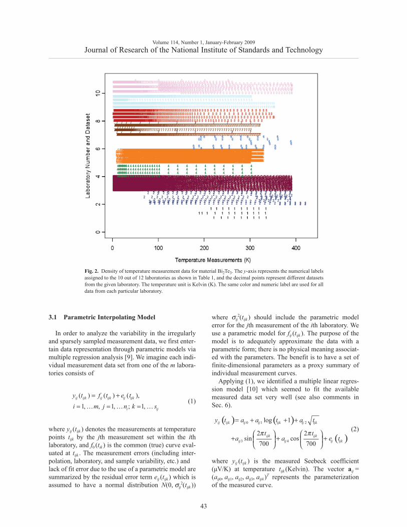
There are issues which present difficulty when analyz-ing and combining measurement data curves fromdifferent measurements, laboratories, or techniques.First, the data covers different temperature ranges withdifferent numbers of sampling points or data density.We assign numerical labels 1, 2, 3, 4, 5, 6, 7, 8, 9, 10for the 10 laboratories whose data are accepted, and weuse decimal points within each interval to representthe different datasets from a particular laboratory. The

temperature sampling points for all measurement data are shown in Fig. 1 for Constantan and Fig. 2 forBi2Te3. Each color/numeric label represents all the data from a particular laboratory. It is seen that the tempera-ture range and density of each measurement data setdiffers greatly between laboratories, and even withinthe same laboratory. These variations cause difficultywhen comparing and combining the different measure-ments. We use a parametric model for the measurementcurves in order to interpolate and to analyze multiplecurves.


42

Fig. 1. Density of temperature measurement data for material Constantan. The y-axis represents the numerical labels assigned to the9 out of 12 laboratories as shown in Table 1, and the decimal points represent different datasets from the given laboratory. The tem-perature unit is Kelvin (K). The same color and numeric label are used for all data from each particular laboratory.

3.1 Parametric Interpolating Model

In order to analyze the variability in the irregularlyand sparsely sampled measurement data, we first enter-tain data representation through parametric models viamultiple regression analysis [9]. We imagine each indi-vidual measurement data set from one of the m labora-tories consists of

(1)

where yij (tijk ) denotes the measurements at temperaturepoints tijk by the jth measurement set within the ithlaboratory, and f0 (tik ) is the common (true) curve eval-uated at tijk . The measurement errors (including inter-polation, laboratory, and sample variability, etc.) and lack of fit error due to the use of a parametric model aresummarized by the residual error term eij (tijk ) which isassumed to have a normal distribution N(0, σij

2(tijk ))

where σij2(tijk ) should include the parametric model

error for the jth measurement of the ith laboratory. Weuse a parametric model for fij (tijk ). The purpose of themodel is to adequately approximate the data with aparametric form; there is no physical meaning associat-ed with the parameters. The benefit is to have a set offinite-dimensional parameters as a proxy summary ofindividual measurement curves.

Applying (1), we identified a multiple linear regres-sion model [10] which seemed to fit the availablemeasured data set very well (see also comments inSec. 6).

(2)

where yij (tijk ) is the measured Seebeck coefficient(μV/K) at temperature tijk (Kelvin). The vector aij =(aij0, aij1, aij2, aij3, aij4 )T represents the parameterizationof the measured curve.


43

Fig. 2. Density of temperature measurement data for material Bi2Te3. The y-axis represents the numerical labelsassigned to the 10 out of 12 laboratories as shown in Table 1, and the decimal points represent different datasetsfrom the given laboratory. The temperature unit is Kelvin (K). The same color and numeric label are used for alldata from each particular laboratory.

( ) ( ) ( ),

1, , 1, ; 1,ij ijk ij ijk ij ijk

i ij

y t f t e t

i m j n k s

= +

= = =… … …

( ) ( )0 1 2log 1ij ijk ij ij ijk ij ijky t a a t a t= + + +

( )3 4

2 2sin cos

700 700ijk ijk

ij ij ij ijk

t ta a e t

π π⎛ ⎞ ⎛ ⎞+ + +⎜ ⎟ ⎜ ⎟

⎝ ⎠ ⎝ ⎠

3.2 Parameter EstimationTo estimate the parameters in Eq. (2) for each data

set, the standard least squares method used in our earli-er work [10] can be improved due to the instabilityin the least squares estimator when the measuredtemperature points are few or limited in a small range.Let X denote the n × p design matrix consisting of5 columns defined by the regression terms in (2) androws which are evaluated at each sampling point. Let Ydenote the Seebeck coefficient response vector. Theleast squares estimator is given by

(3)

The problem with the standard least squares methodapplying to (2) is that X TX is near singular when thesample size is small or the temperature measurementrange is narrow. As a consequence, the estimatedparameters can be highly variable and unstable; and theuncertainties associated with the estimated parametersare extremely large. To alleviate the problem one canuse the Ridge regression method [11] by introductionof smoothing parameter k to stabilize the inversecomputation given by

(4)

If we denote the singular value decomposition of X byX = UDV T, then X T X = VD 2V T,

(5)

(6)

Also, if we denote A(k) = UD(D2 + kI )–1 DU T, thenYR = A(k)Y .

The choice of k requires careful considerations. Alarge k reduces the variance in the resulting estimatorwhile incurring potentially large bias. We try to select kthat gives a stable estimator and has negligible bias. Aformal procedure for choosing k is based on theGeneralized Cross-validation criterion [12] by mini-mizing the prediction variance

(7)

In practice, we find that the smallest k among thefeasible values is always preferred. This indicates thatour chosen estimators are close to those given byusing the generalized inverses. If we let X + denotethe Moore-Penrose inverse of a matrix X, then X + =(X TX)+X T; and X + satisfies the following conditions[13]:

(8)

(9)

If X = UDV T, then X + = VD +U T where D + is the trans-pose of D whose positive singular values are replacedby their reciprocals. When k → 0, the Ridge regressionestimator in (4) converges to the Moore-Penrose gener-alized inverse estimator given by:

(10)

The estimator is a least squares solution to the follow-ing problem: its norm ||β || 2 is minimized among allvectors β for which

(11)

is minimized. The corresponding fitted regression lineis given by

(12)

(13)

where we assume Cov (Y ) = σ 2 I. Note that the Ridgeregression estimator may be biased. A useful notion isestimable function (or linear combination of para-meters) for which there exists unbiased estimate basedon linear combination of data. This is the essence of the


44

( ) 1ˆ ˆˆ; .T TX X X Y Y Xβ β−

= =

( ) 1ˆ ˆˆ; .T TR R RX X kI X Y Y Xβ β

−= + =

( ) ( )1 12 2ˆ T T TR VD V kI VDU Y V D kI DU Yβ

− −= + = +

( )21

pTii i

i i

u Y Vk

δδ=

⎛ ⎞= ⎜ ⎟+⎝ ⎠

∑

{ }1 1 1where ,..., , U=(u ,..., ), ( ,..., )p p pD diag u V V Vδ δ= =

( ) ( )2

122

1

ˆ .p

T TiR i i

i i

Y UD D kI DU Y u Y uk

δδ

−

=

⎛ ⎞= + = ⎜ ⎟+⎝ ⎠

∑

and

( )( )( )

( )( )

2

2

1

1

I A k Ynk

tr I A kn

−Ω =

⎡ ⎤−⎢ ⎥⎣ ⎦

( )( )

( )2 2

2221 1

2

2

21

.11

pni i T

i ii i i

i

ky u Y

n k

p kn n k

δ δ

δ

δ

= =

⎡ ⎤+⎢ ⎥−⎢ ⎥+⎣ ⎦=

⎡ ⎤− +⎢ ⎥+⎣ ⎦

∑ ∑

, are symmetricX X XX+ +

, .XX X X X XX X+ + + += =

( )ˆ .T TX Y X X X Yβ++

+ = =

2Y X β−

( )ˆ .T TY X X X X Y XX Y+ +

+ = =

ˆThe covariance of is given byβ+

2ˆ( ) ( )TCov X Xβ σ ++ =

theory of the Gauss-Markov model and for estimablefunctions there are simplifying expressions for uncer-tainty analysis [14].

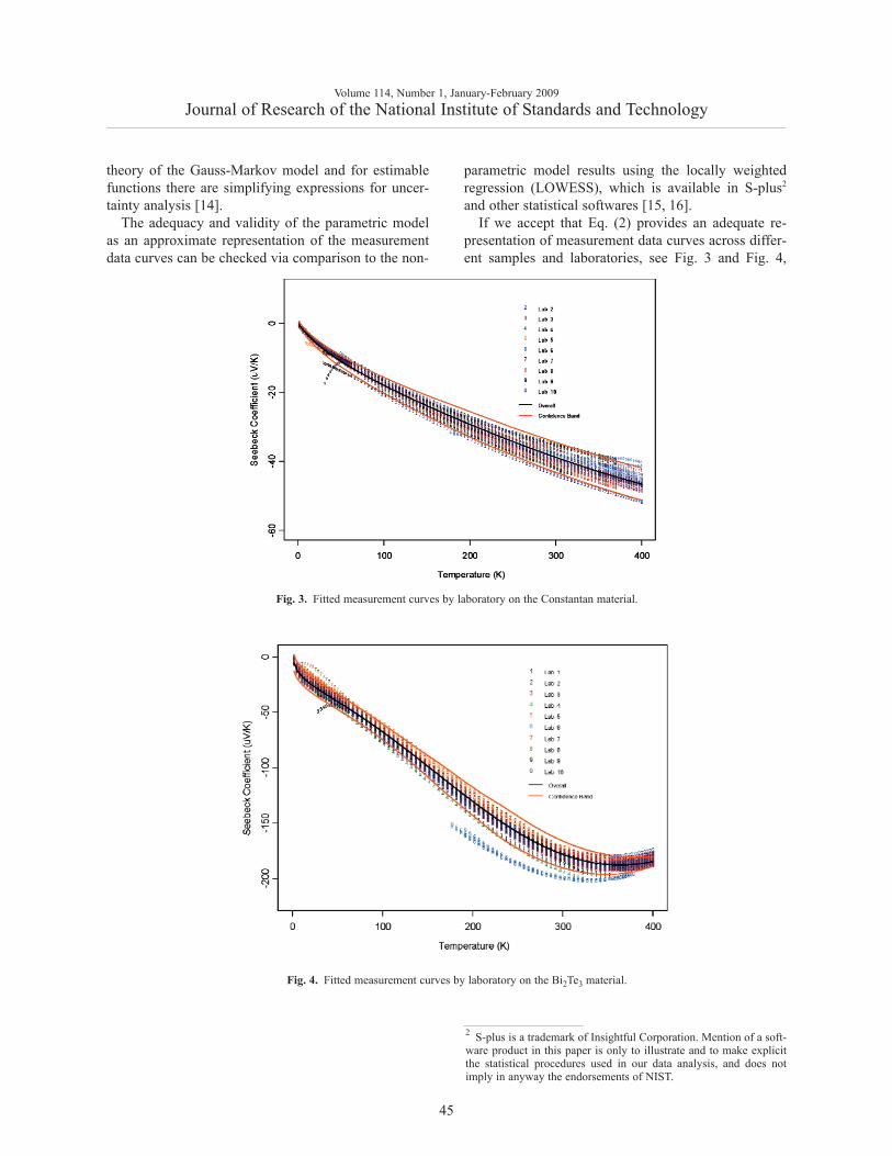
The adequacy and validity of the parametric modelas an approximate representation of the measurementdata curves can be checked via comparison to the non-

parametric model results using the locally weightedregression (LOWESS), which is available in S-plus2

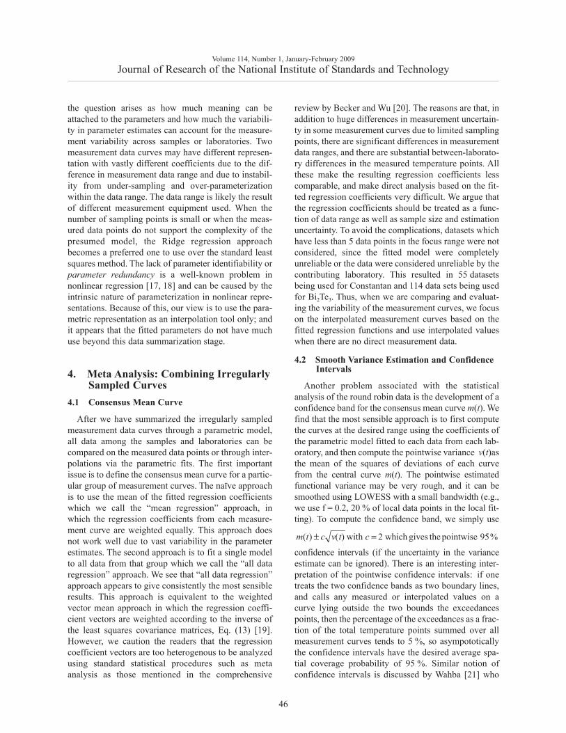
and other statistical softwares [15, 16].If we accept that Eq. (2) provides an adequate re-

presentation of measurement data curves across differ-ent samples and laboratories, see Fig. 3 and Fig. 4,


45

2 S-plus is a trademark of Insightful Corporation. Mention of a soft-ware product in this paper is only to illustrate and to make explicitthe statistical procedures used in our data analysis, and does notimply in anyway the endorsements of NIST.

Fig. 3. Fitted measurement curves by laboratory on the Constantan material.

Fig. 4. Fitted measurement curves by laboratory on the Bi2Te3 material.

the question arises as how much meaning can beattached to the parameters and how much the variabili-ty in parameter estimates can account for the measure-ment variability across samples or laboratories. Twomeasurement data curves may have different represen-tation with vastly different coefficients due to the dif-ference in measurement data range and due to instabil-ity from under-sampling and over-parameterizationwithin the data range. The data range is likely the resultof different measurement equipment used. When thenumber of sampling points is small or when the meas-ured data points do not support the complexity of thepresumed model, the Ridge regression approachbecomes a preferred one to use over the standard leastsquares method. The lack of parameter identifiability orparameter redundancy is a well-known problem innonlinear regression [17, 18] and can be caused by theintrinsic nature of parameterization in nonlinear repre-sentations. Because of this, our view is to use the para-metric representation as an interpolation tool only; andit appears that the fitted parameters do not have muchuse beyond this data summarization stage.

4. Meta Analysis: Combining IrregularlySampled Curves

4.1 Consensus Mean Curve

After we have summarized the irregularly sampledmeasurement data curves through a parametric model,all data among the samples and laboratories can becompared on the measured data points or through inter-polations via the parametric fits. The first importantissue is to define the consensus mean curve for a partic-ular group of measurement curves. The naïve approachis to use the mean of the fitted regression coefficientswhich we call the “mean regression” approach, inwhich the regression coefficients from each measure-ment curve are weighted equally. This approach doesnot work well due to vast variability in the parameterestimates. The second approach is to fit a single modelto all data from that group which we call the “all dataregression” approach. We see that “all data regression”approach appears to give consistently the most sensibleresults. This approach is equivalent to the weightedvector mean approach in which the regression coeffi-cient vectors are weighted according to the inverse ofthe least squares covariance matrices, Eq. (13) [19].However, we caution the readers that the regressioncoefficient vectors are too heterogenous to be analyzedusing standard statistical procedures such as metaanalysis as those mentioned in the comprehensive

review by Becker and Wu [20]. The reasons are that, inaddition to huge differences in measurement uncertain-ty in some measurement curves due to limited samplingpoints, there are significant differences in measurementdata ranges, and there are substantial between-laborato-ry differences in the measured temperature points. Allthese make the resulting regression coefficients lesscomparable, and make direct analysis based on the fit-ted regression coefficients very difficult. We argue thatthe regression coefficients should be treated as a func-tion of data range as well as sample size and estimationuncertainty. To avoid the complications, datasets whichhave less than 5 data points in the focus range were notconsidered, since the fitted model were completelyunreliable or the data were considered unreliable by thecontributing laboratory. This resulted in 55 datasetsbeing used for Constantan and 114 data sets being usedfor Bi2Te3. Thus, when we are comparing and evaluat-ing the variability of the measurement curves, we focuson the interpolated measurement curves based on thefitted regression functions and use interpolated valueswhen there are no direct measurement data.

4.2 Smooth Variance Estimation and Confidence Intervals

Another problem associated with the statisticalanalysis of the round robin data is the development of aconfidence band for the consensus mean curve m(t). Wefind that the most sensible approach is to first computethe curves at the desired range using the coefficients ofthe parametric model fitted to each data from each lab-oratory, and then compute the pointwise variance v(t)asthe mean of the squares of deviations of each curvefrom the central curve m(t). The pointwise estimatedfunctional variance may be very rough, and it can besmoothed using LOWESS with a small bandwidth (e.g.,we use f = 0.2, 20 % of local data points in the local fit-ting). To compute the confidence band, we simply use

confidence intervals (if the uncertainty in the varianceestimate can be ignored). There is an interesting inter-pretation of the pointwise confidence intervals: if onetreats the two confidence bands as two boundary lines,and calls any measured or interpolated values on acurve lying outside the two bounds the exceedancespoints, then the percentage of the exceedances as a frac-tion of the total temperature points summed over allmeasurement curves tends to 5 %, so asympototicallythe confidence intervals have the desired average spa-tial coverage probability of 95 %. Similar notion ofconfidence intervals is discussed by Wahba [21] who


46

( ) ( ) with 2 which gives the pointwise 95%m t c v t c± =

also coined the name of Bayesian confidence intervals,and by Nychka [22] who proved that the pointwiseconfidence intervals in the context of a smoothingspline regression has the required specified averagecoverage probability.

5. Statistical Analysis Results

Using the “all data regression” approach and Eq. (2),we modeled all data for the 2 candidate materials whichgave

(14)

for Constantan and

(15)

for Bi2Te3. These results are plotted in Figs. 3 and 4respectively with all the data used for the model.

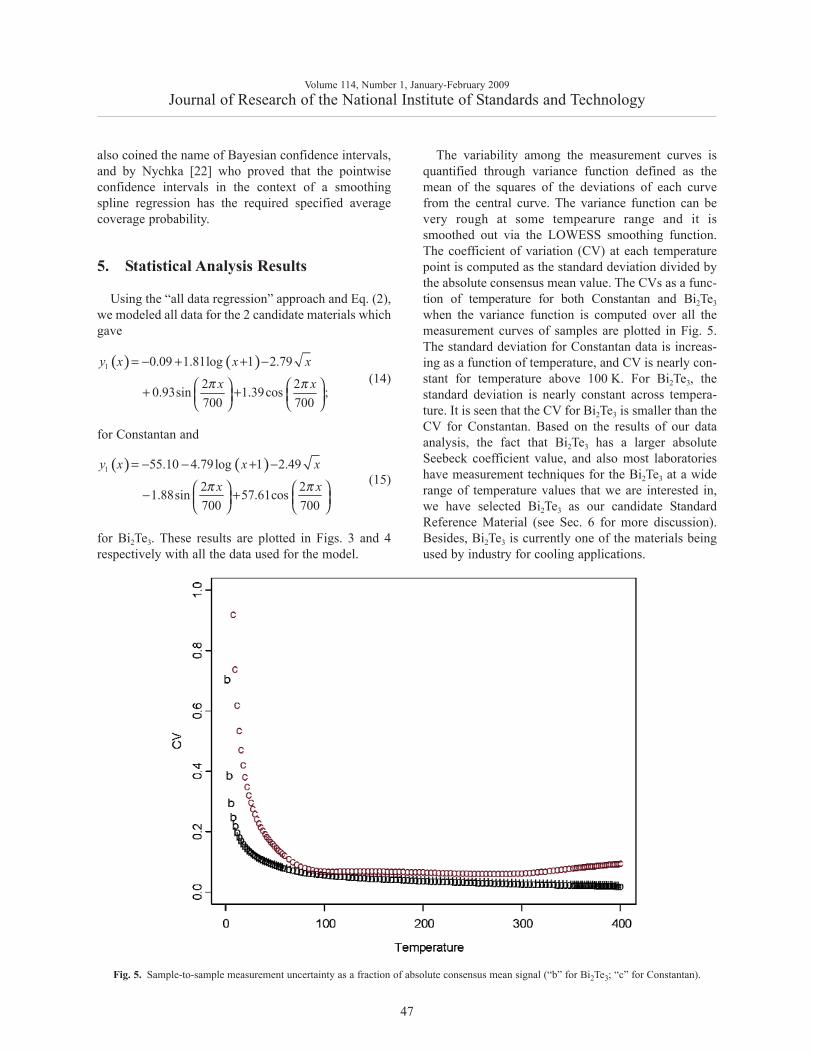
The variability among the measurement curves isquantified through variance function defined as themean of the squares of the deviations of each curvefrom the central curve. The variance function can bevery rough at some tempearure range and it issmoothed out via the LOWESS smoothing function.The coefficient of variation (CV) at each temperaturepoint is computed as the standard deviation divided bythe absolute consensus mean value. The CVs as a func-tion of temperature for both Constantan and Bi2Te3

when the variance function is computed over all themeasurement curves of samples are plotted in Fig. 5.The standard deviation for Constantan data is increas-ing as a function of temperature, and CV is nearly con-stant for temperature above 100 K. For Bi2Te3, thestandard deviation is nearly constant across tempera-ture. It is seen that the CV for Bi2Te3 is smaller than theCV for Constantan. Based on the results of our dataanalysis, the fact that Bi2Te3 has a larger absoluteSeebeck coefficient value, and also most laboratorieshave measurement techniques for the Bi2Te3 at a widerange of temperature values that we are interested in,we have selected Bi2Te3 as our candidate StandardReference Material (see Sec. 6 for more discussion).Besides, Bi2Te3 is currently one of the materials beingused by industry for cooling applications.


47

( ) ( )1 0.09 1.81log 1 2.79

2 20.93sin 1.39cos ;700 700

y x x x

x xπ π

= − + + −

⎛ ⎞ ⎛ ⎞+ +⎜ ⎟ ⎜ ⎟⎝ ⎠ ⎝ ⎠

( ) ( )1 55.10 4.79log 1 2.49

2 21.88sin 57.61cos700 700

y x x x

x xπ π

= − − + −

⎛ ⎞ ⎛ ⎞− +⎜ ⎟ ⎜ ⎟⎝ ⎠ ⎝ ⎠

Fig. 5. Sample-to-sample measurement uncertainty as a fraction of absolute consensus mean signal (“b” for Bi2Te3; “c” for Constantan).

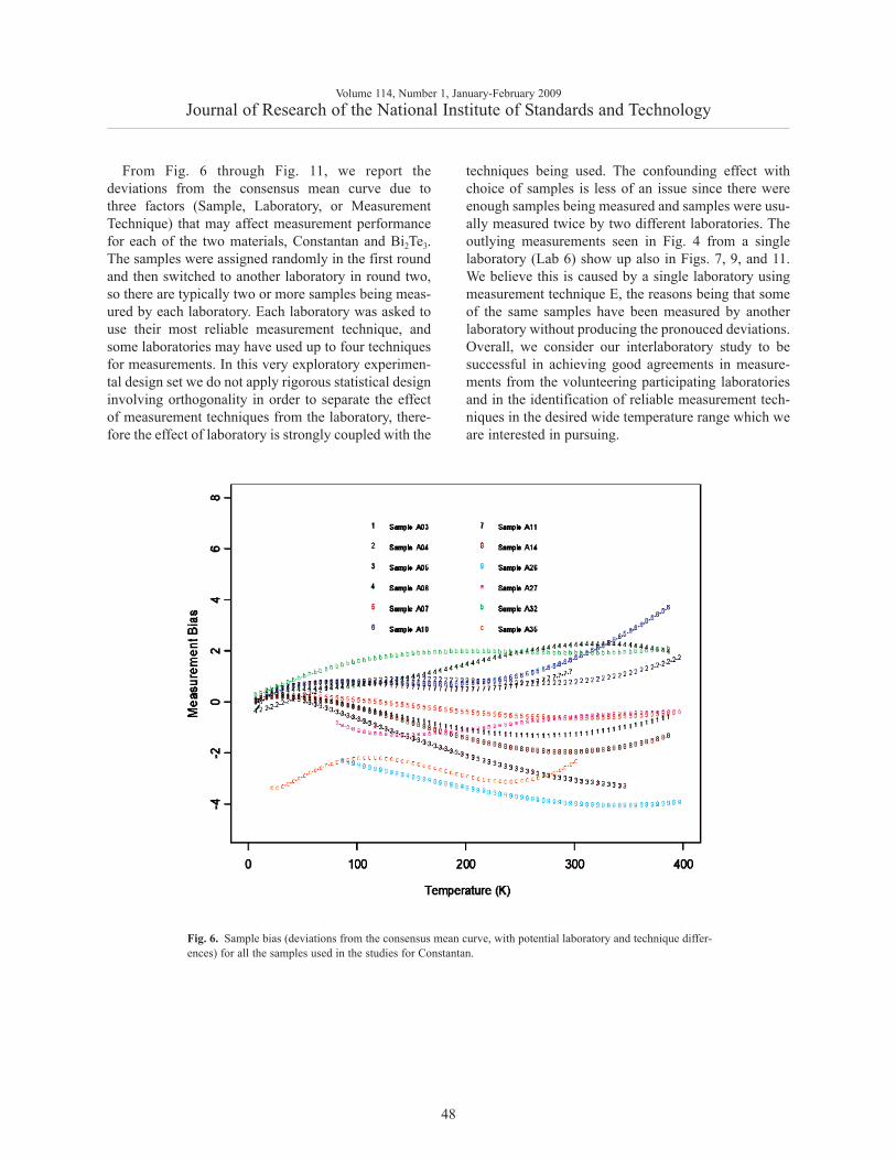
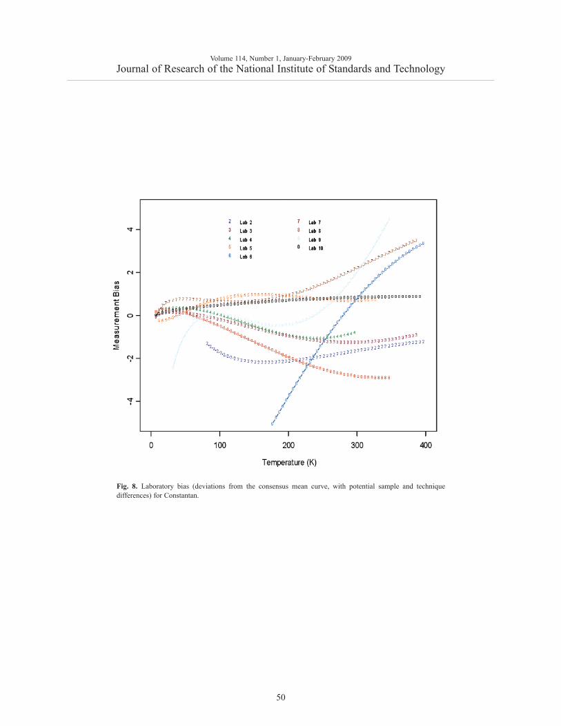
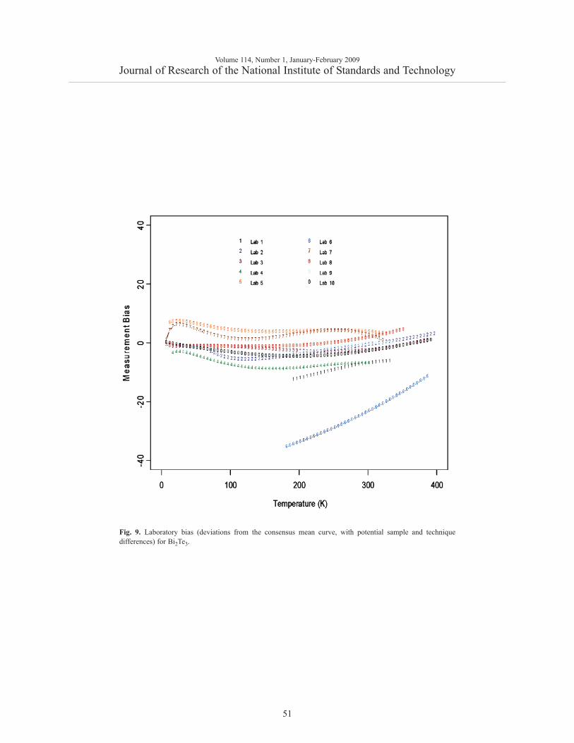
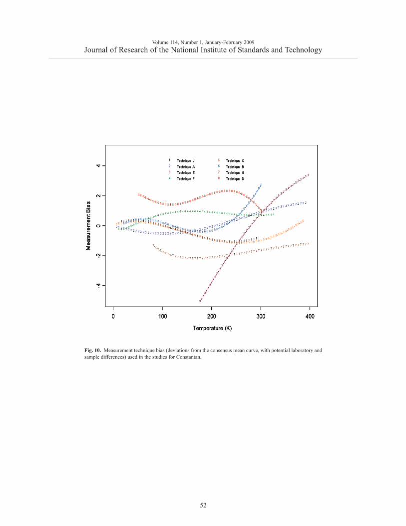
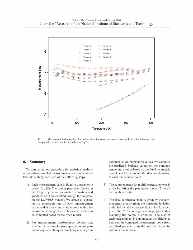
From Fig. 6 through Fig. 11, we report thedeviations from the consensus mean curve due tothree factors (Sample, Laboratory, or MeasurementTechnique) that may affect measurement performancefor each of the two materials, Constantan and Bi2Te3.The samples were assigned randomly in the first roundand then switched to another laboratory in round two,so there are typically two or more samples being meas-ured by each laboratory. Each laboratory was asked touse their most reliable measurement technique, andsome laboratories may have used up to four techniquesfor measurements. In this very exploratory experimen-tal design set we do not apply rigorous statistical designinvolving orthogonality in order to separate the effectof measurement techniques from the laboratory, there-fore the effect of laboratory is strongly coupled with the

techniques being used. The confounding effect withchoice of samples is less of an issue since there wereenough samples being measured and samples were usu-ally measured twice by two different laboratories. Theoutlying measurements seen in Fig. 4 from a singlelaboratory (Lab 6) show up also in Figs. 7, 9, and 11.We believe this is caused by a single laboratory usingmeasurement technique E, the reasons being that someof the same samples have been measured by anotherlaboratory without producing the pronouced deviations.Overall, we consider our interlaboratory study to besuccessful in achieving good agreements in measure-ments from the volunteering participating laboratoriesand in the identification of reliable measurement tech-niques in the desired wide temperature range which weare interested in pursuing.


48

Fig. 6. Sample bias (deviations from the consensus mean curve, with potential laboratory and technique differ-ences) for all the samples used in the studies for Constantan.


49

Fig. 7. Sample bias (deviations from the consensus mean curve, with potential laboratory and technique differ-ences) for all the samples used in the studies for Bi2Te3.


50

Fig. 8. Laboratory bias (deviations from the consensus mean curve, with potential sample and techniquedifferences) for Constantan.


51

Fig. 9. Laboratory bias (deviations from the consensus mean curve, with potential sample and techniquedifferences) for Bi2Te3.


52

Fig. 10. Measurement technique bias (deviations from the consensus mean curve, with potential laboratory andsample differences) used in the studies for Constantan.

6. Summary

To summarize, our procedure for statistical analysisof irregularly sampled measurement curves in the inter-laboratory study consisted of the following steps.

1) Each measurement data is fitted to a parametricmodel Eq. (2). The tuning parameter choice inthe Ridge regression parameter estimation andgoodness of fit are checked through the nonpara-metric LOWESS models. We arrive at a para-metric representation of each measurementcurve; and at every temperature point within themeasurement range, the Seebeck coefficient canbe computed based on the fitted model.

2) For measurement performance comparison,whether it is sample-to-sample, laboratory-to-laboratory, or technique-to-technique, at a given

common set of temperature values, we compute the predicted Seebeck values on the commontemperature points based on the fitted parametricmodel, and then compute the standard deviationat each temperature point.

3) The common mean for multiple measurements isgiven by fitting the parametric model (2) to allthe combined data.

4) The final confidence band is given by the com-mon mean plus or minus the stanadard deviationmultipled by the coverage factor k = 2, whichgives the 95 % average coverage probabilityassuming the normal distribution. The bias ofeach measurement is computed as the differencebetween the computed measurement point fromthe fitted parametric model and that from thecommon mean model.


53

Fig. 11. Measurement technique bias (deviations from the consensus mean curve, with potential laboratory andsample differences) used in the studies for Bi2Te3.

Our study offers a few lessons which may be benefi-cial for future design and analysis of interlaboratoryexperiments involving sampled curves and functions.The significant differences (cf. Fig. 1 and Fig. 2) in thesampling design from different laboratories and differ-ent replicates have made analysis based on the para-meters of an interpolating model unsuitable. Weemphasize that the proposed model (2) is just one ofthe many interpolating models that can be used. Forexample, we have recently discovered another model inour latest Seebeck coefficient SRM work,

(16)

which also fits the round robin data well. However, weshould point out that fitting of this model to the roundrobin data still presents the same challenges as the lin-ear terms cannot be reformulated into orthogonal termsbecause of the vast differences in the sampling designof each data set, and orthogonality depends on thedesign of data sets. The strong multicollearity in theless sampled data set makes the use of Ridge regressionnecessary, though it is more difficult to compare thedifferent data sets based on the fitted parameters. Thatis the reason why we emphasize that the parametricmodel has served our purpose of interpolation withineach data set very well, but the fitted parameters haveno physical meanings and have vast variations acrossdifferent data sets. Another important lesson is that, wehave not enforced a good statistical design so that theconfounding effect of measurement technique and lab-oratory effects may be reduced. In the future whenthere are more laboratories who can use multiple tech-niques, a good choice of experimental design maybecome feasible.

Based on the results of the round-robin measurementsurvey, Bi2Te3 will be used for the SRM. To this end,400 units have been purchased from Marlow Industrieswith sample dimensions of 8 mm × 3.5 mm × 2.5 mm.This sample has different dimensions than those usedfor the round-robin measurement survey based on feed-back from the participants. These dimensions allowmore room for 4-probe resistivity measurements whilemaintaining an appropriate thermal conductance.

Bi2Te3 will be certified as the SRM at NIST with thestandard data produced using a Quantum DesignPhysical Property Measurement System with somemodifications including 3rd party electronics andcustom software. The details of this system and tech-nique will be discussed elsewhere.

7. References

[1] T. J. Seebeck, Magnetic polarization of metals and minerals,Abhandlungen der Deutschen Akademie der Wissenschaften zuBerlin, 265 (1822).

[2] J. C. Peltier, Nouvelles experiences sur la caloricite des couranselectrique, Ann. Chim. LV1 371 (1834).

[3] T. M. Tritt, Thermoelectrics Run Hot and Cold, Science 272,1276-1277 (1996).

[4] R. Venkatasubramanian, E. Siivola, T. Colpitts, and B.O’Quinn, Thin-film thermoelectric devices with highroom-temperature figures of merit, Nature 413, 597-602(2001).

[5] Kuei Fang Hsu, Sim Loo, Fu Guo, Wei Chen, Jeffrey S. Dyck,Ctirad Uher, Tim Hogan, E. K. Polychroniadis, and Mercouri G.Kanatzidis, Cubic AgPbmSbTe2+m: Bulk ThermoelectricMaterials with High Figure of Merit, Science 303, 818-821(2004).

[6] Brian C. Sales, Electron Crystals and Phonon Glasses: A NewPath to Improved Thermoelectric Materials, MRS Bulletin, 23,15 (1998).

[7] R. T. Littleton, IV, An Investigation of Transition MetalPentatellurides as a Potential Low-temperature Thermo-electric Refrigeration Material, Ph. D. Dissertation, ClemsonUniversity (2001).

[8] NIST Standard Reference Materials Home Page,http://ts.nist.gov/ts/htdocs/230/232/232.htm.

[9] N. R. Draper and H. Smith, Applied Regression Analysis, 2ndEd., John Wiley & Sons (1981), pp. 218-293.

[10] N. D. Lowhorn, W. Wong-Ng, W. Zhang, Z.Q. Lu et al., Round-robin studies of two Potential Seebeck coefficientstandard reference materials. Appl. Physics A 94, 231-234(2009).

[11] A. E. Hoerl and R.W. Kennard (1970). Ridge regression:biased estimation for nonorthogonal problems. Technometrics,Vol.12, No.1, pp.55-67.

[12] G. H. Golub, M. Heath, and G. Wahba (1979). Generalizedcross-validation as a method for choosing a good Ridge para-meter. Technometrics, Vol.21, No.2, pp.215-223.

[13] A. Albert, Regression and the Moore-Penrose Pseudoinverse.Academic Press, New York and London, pg. 26-28 (1972).

[14] C. R. Rao and S. K. Mitra (1971). Generalized Inverse ofMatrices and its Applications. John Wiley & Sons, Inc., NewYork, pg. 139-141, Theorem 7.2.1, Theorem 7.2.3.

[15] W. S. Cleveland, Robust locally weighted regression andsmoothing scatterplots. Journal of the American StatisticalAssociation 74, 829-836 (1979).

[16] W. S. Cleveland, LOWESS: A program for smoothing scatter-plots by robust locally weighted regression. The AmericanStatistician, Vol.35, No.1, p.54-54 (1981).

[17] G A. F. Seber and C. J. Wild (1989). Nonlinear Regression.Wiley, New York, Section 3.4.

[18] J. G. Reich, On parameter redundancy in curve fitting of kinet-ic data. In L. Endrenyi (ed.), Kinetic Data Analysis: Designand Analysis of Enzyme and Pharmacokinetic Experiments,pp.39-50, Plenum Press, New York (1981).

[19] A. L. Rukhin, Estimating common vector parameters in inter-laboratory studies. Journal of Multivariate Analysis, Vol. 98,435-454 (2007).

[20] B. J. Becker and M.-J. Wu (2007). The synthesis of regressionslopes in meta-analysis. Statistical Science, Vol.22, No.3, 414-429.


54

20 1 2

3 43 4

( ) ( 200)

( 200) ( 200)

m t a a t a t

a t a t

= + + −

+ − + −

[21] G. Wahba (1983). Bayesian “Confidence Intervals” for theCross-validated Smoothing Spline. Journal of Royal StatisticalSociety B, Vol.45, No.1, pp.133-150.

[22] D. Nychka, Bayesian Confidence Intervals for SmoothingSplines. Journal of American Statistical Association, Vol.83,No.404, pp.1134-1143 (1988).

About the authors: Z. Q. John Lu is a mathematicalstatistician in the Statistical Engineering Division ofthe NIST Information Technology Laboratory.

Nathan D. Lowhorn was a guest researcher at NIST;currently he is an adjunct professor in the PhysicsDepartment at Middle Tennessee State University.

Winnie Wong-Ng is a member of the FunctionalProperties group of the Ceramics Division, NIST; she isthe leader of the “Measurements and Standards forEnergy Conversion Materials” project.

Weiping Zhang was a guest researcher in theStatistical Engineering Division of NIST; currently heis an assistant professor in the Department of Statisticsand Finance of the University of Science andTechnology of China.

Makoto Otani was a previous guest researcher at theFunctional Properties group of the Ceramics Divisionat NIST; currently he is working for Honda R&D,Japan.

Evan E. Thomas is a NRC research associate at theFunctional Properties group of the Ceramics Division,NIST.

Martin L. Green is the group leader of theFunctional Properties group of the Ceramics Division,NIST.

Thanh N. Tran is a senior scientist at the PowerSources R&D Group of the Naval Surface WarfareCenter, Carderock.

Christopher Caylor is the manager ofThermoelectric Power Programs in the Center forSolid-State Energetics at RTI International in ResearchTriangle Park, NC.

Neil R. Dilley is an applications physicist workingfor Quantum Design and was on the development teamfor their Thermal Transport measurement option.

B. Edwards is previous graduate student at thePhysics Department of Clemson University and nowworks as an Engineer for General Electric inGreenville, SC.

N. Elsner is the president of Hi-Z Technology, Inc.and is responsible for the overall materials effort in(Bi,Sb)2(Se,Te)3, PbTe and Quantum Well materialssuch as Si/SiGe.

S. Ghamaty is a project manager at Hi-Z Technology,Inc. and is pursuing the development and qualificationof the very promising Quantum Well materials.

Timothy P. Hogan is an Associate Professor in theElectrical and Computer Engineering, and ChemicalEngineering and Materials Science Departments,Michigan State University.

Adams D. Downey was a graduate student in theElectrical and Computer Engineering Department atMichigan State University; he is presently an associateproject manager at Stryker Medical in Portage, MI.

Qiang Li is the superconducting and thermoelectricmaterials group leader in the Condensed MatterPhysics and Materials Science Department ofBrookhaven National Laboratory, and AdjunctProfessor of Materials Science and EngineeringDepartment of State University of New York at StonyBrook.

Qing Jie is a Ph.D graduate student of MaterialsScience andEngineering Department of StateUniversity of New York at Stony Brook, and works inthe Condensed Matter Physics and Materials ScienceDepartment of Brookhaven National Laboratory underthe supervision of Qiang Li.

Joshua Martin was a graduate student of ProfessorGeorge Nolas at the Physics Department of Unviersityof South Florida; currently he is a NRC research asso-ciate with the Ceramics Division of NIST

George Nolas is an Associate Professor at thePhysics Department of University of South Florida.

Haruhiko Obara is a group leader of theThermoelectric Energy Conversion Group in theAdvanced Industrial Science and Technology (AIST),Tsukuba, Japan.

Jeffrey Sharp is Chief Scientist and Sr. Manager ofMaterials R&D at Marlow Industries, Inc., a sub-sidiary of II-VI Incorporated.

Rama Venkatasubramanian is the Research Directorof the Center for Solid State Energetics at RTIInternational in Research Triangle Park, NC.

Rhonda Willigan is a principal investigator workingin the Physical Sciences Department of the UnitedTechnologies Research Center.

Jihui Yang is a senior scientist at the General MotorsR&D Center.

Terry M. Tritt is a Professor of Physics at ClemsonUniversity with extensive expertise in thermoelectricmaterials as well as thermoelectric measurements andheads up Clemson’s Complex and Advanced MaterialsLaboratory.

The National Institute of Standards and Technologyis an agency of the U.S. Department of Commerce.


55

Documents

Statistical Analysis of a Round-Robin Measurement Survey ... · RTI International, Research Triangle Park, NC 27709 R. Willigan United Technologies Research Center, ... resurgence