Statistical calibration of 2DOF vortex-induced vibration

24th ABCM International Congress of Mechanical EngineeringDecember 3-8, 2017, Curitiba, PR, Brazil

Statistical calibration of 2DOF vortex-induced vibrationphenomenological model.

Gabriel M. GuerraRodolfo FreitasBruno SoaresFernando A. [email protected] Engineering Department, Federal University of Rio de Janeiro, Rio de Janeiro, Brazil, [email protected]

Abstract. The vortex-induced vibrations of floating structures play an important role in the design of offshore engineering.The accurate prediction of structural instability is extremely important due that the vortex shedding behind bluff bodiesmay lead to degradation of structural performance or even structural failure. Analytical VIV models can be representedby numerous approaches to modeling both the structure and fluid. The CFD (Computational Fluid Dynamics) approachesconsists of solving the Navier-Stokes equations directly, mostly limited by heavily computational costs that many timesvery difficult to satisfy in the practical engineering. In this sense, semi-empirical models are an alternative approach,where the fluid dynamic forces acting on the structure are emulated by phenomenological equations and can be a veryuseful tool in wide industrial applications. The purpose this work is to present a phenomenological model of vortex-induced vibrations for spring-mounted rigid cylinder structures putting the parameter variability in the general contextof Uncertainty Analysis doing first a sensitivity analysis for input empirical parameters of the model using the AdaptiveSparse Grid Stochastic Collocation method (ASGSC). After this, a backward parameter estimation analysis is done using aBayesian technique to calibrate these empirical parameters, by means of exploring posterior density functions. Syntheticdata were generated as reference simulating experimental data to show the calibration technique used. This kind ofanalysis can help to understand the behavior of the structure to critical situations as well the effects of varying empiricalparameters in the response variables. The influence of these parameters and other coefficients that affect the dynamicalresponse is analyzed and also discussed.Vortex induced vibrations, Reduced model, Calibration

1. INTRODUCTION

Vortex-Induced Vibration are motions induced on bodies interacting with an external fluid flow, it is caused by thevortex shedding behind bluff bodies and may lead to degradation of structural performance or even structural failure. Inoffshore structures such as pipes, risers and mooring lines, it is a particularly important. Exist several ways to predict thedynamic response of structures undergoing large amplitude vibrations induced by the surrounding flow. One of the mosteffective prediction method consists of solving the coupled fluid-structure system modeling the flow through Navier-Stokes equations where the structure, due to its rigidity, can be characterized by a simple oscillator with one or twodegrees of freedom. The main problem is that the complexity involved in solving these systems generally leads to the useof simpler computational models, as a preliminary approach, due to the prohibitive costs of considering more complexsystems in the preliminary phase of the project. Thus, an alternative, is to use a phenomenological model based on wakeoscillators Gabbai and Benaroya (2005) that replace the vortex shedding mechanisms of the flow by simple models. Inthis work we present a model proposed in Postnikov et al. (2017) that captures important features of the VIV dynamics2DOF. Another problem that appears is the reliability of those simulations many time is disrupted by the inexorablepresence of uncertainty in the model data, such as inexact knowledge of system forcing, initial and boundary conditions,physical properties of the medium, as well as parameters in constitutive equations. These situations underscore the needfor efficient uncertainty quantification methods for the establishment of confidence intervals in computed predictions, theassessment of the suitability of model formulations, and/or the support of decision-making analysis.

In this sense, traditional statistical tool for uncertainty quantification within the realm of Engineering is the MonteCarlo method, see Elishakoff (2003). This method requires, first, the generation of an ensemble of random realizationsassociated with the uncertain data, and then it employs deterministic solvers repetitively to obtain the ensemble of results.The ensemble results should be processed to estimate the mean and standard deviation of the final results. The implemen-tation the Monte Carlo is straightforward, but its convergence rate is very slow (proportional to the inverse of the squareroot of the realization number) and often infeasible due the large CPU time needed to run the model in question. Anothertechnique that has been applied recently is the so-called Stochastic Galerkin Method (SG), which employs Polynomial

F. Author, S. Author and T. Author (update this heading accordingly)Paper Short Title (First Letters Uppercase, make sure it fits in one line)

Chaos expansions to represent the solution and inputs to stochastic differential equations, see Babuska et al. (2004). Anon-intrusive method, referred to as Stochastic Collocation (SC), see Xiu and Hesthaven (2005), arises addressing as acombination of interpolation methods and deterministic solvers, like Monte Carlo where a deterministic problem is solvedat each point of an abstract random space. Similarly to SG methods, SC methods achieve fast convergence when the solu-tion possesses sufficient smoothness in random space. Thus when there are steeps gradients or finite discontinuities in thestochastic space, these methods converge very slowly or even fail to converge. In this work, we present an adaptive sparsegrid collocation strategy with the aim of obtaining greater accuracy in nonlinear systems analysis. Specifically, it will beexamined an interesting situation involving fluid-structure interaction in a model used as preliminary approach of Engi-neering projects.The analysis done takes into account uncertainties in the coupling parameters of the model. Thus, for theforward sensitivity analyzes, the problem is then formulated through the probabilistic approach where the uncertaintiesare characterized by a probability density function. Particular emphasis is placed on investigating uncertainty propagationin the nonlinear response of fluid-structure interaction, see Xiu et al. (2002). The Stochastic Collocation method is usedto propagate uncertainties through the model offering an appropriate framework to tackle the external forces and uncer-tainties in the input data. Here, the fluid-structure interaction is modeled in a simple way focusing the assessment of anSC method as an effective tool for uncertainty quantification. Results are presented as errorbars for inline and crossflowthe amplitude for a reduced velocity range.

2. MATHEMATICAL MODEL

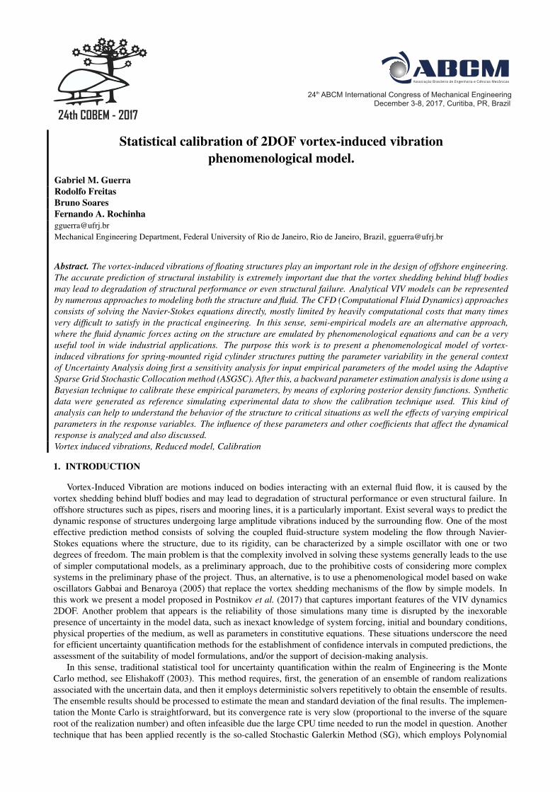
The problem of this approach, when applied to real problems is that sometime lead in to highly cost models for UQanalysis or in preliminary phase os design. An alternative, is to use a phenomenological model based on wake oscillatorsGabbai and Benaroya (2005) that replace the vortex shedding mechanisms of the flow by simple models. In this examplewe use a similar model as presented in Kreuzer (2008) and Rosetti et al. (2011) that captures important features of the VIVdynamics after a calibration of its parameters, taking into consideration the available experimental data. Due this reason,the calibration is an activity that leads with parameters subject to uncertainties that can be modeled using experimentaldata as references solution to analyse the parameters of our phenomenological model with the following equations model.Thus considering an elastically supported rigid circular cylinder shown schematically in Fig. 1.

Figure 1: Computational setup in our study

Based on the classical Van der-pol equation, with empirical parameters, this system can emulate the fluid dynamicsaround the body to predict the behavior of the system. The scheme of the coupling wake and structure oscillator isrepresented by the following equations,

mx+ rsx+ hx =1

2ρfCLD|UR|y +

1

2ρfCDD|UR|(U − x)

my + rsy + hy =1

2ρfCLD|UR|(U − x) +

1

2ρfCDD|UR|y

w + 2εxΩF (w2 − 1)w + 4Ω2Fw = (Ax/D)x

q + εyΩF (q2 − 1)q + Ω2F q = (Ay/D)y

24th ABCM International Congress of Mechanical Engineering (COBEM 2017)December 3-8, 2017, Curitiba, PR, Brazil

where

|UR| =√

(U − x)2 + y2

CL =CL0

q

2

CD = CD0(1 +Kq2) +

CflD

2

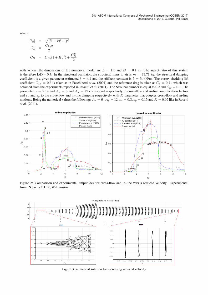
with Where, the dimensions of the numerical model are L = 1m and D = 0.1 m. The aspect ratio of this systemis therefore L/D = 0.4. In the structural oscillator, the structural mass in air is m = 45.71 kg; the structural dampingcoefficient is a given parameter estimated ξ = 4.4 and the stiffness constant is k = 5. kN/m. The vortex shedding liftcoefficient CLo = 0.3 is taken as in Facchinetti et al. (2004) and the reference drag is taken as Co = 0.7 , which wasobtained from the experiments reported in Rosetti et al. (2011). The Strouhal number is equal to 0.2 and Cio = 0.1. Theparameter γ = 2.14 and Ax = 8 and Ay = 42 correspond respectively to cross-flow and in-line amplification factorsand εx and εy to the cross-flow and in-line damping respectively with K parameter that couples cross-flow and in-linemotions. Being the numerical values the followingsAx = 6 , Ay = 12, εx = 0.3, εy = 0.15 andK = 0.05 like in Rosettiet al. (2011).

Figure 2: Comparison and experimental amplitudes for cross-flow and in-line versus reduced velocity. Experimentalfrom: N.Javtis C.H.K, Williamson

Figure 3: numerical solution for increasing reduced velocity


3. SENSITIVITY ANALYSIS

3.1 Adaptive sparse grid stochastic collocation method

The main idea of this method is approximate the multidimensional stochastic space building a interpolation functionon a set of collocation points YiMi=1 in the stochastic space Γ ⊂ RM . The method, similarly to Monte Carlo methods,requires only the solution of a set of decoupled equations, allowing the model to be treated as a black box and solved it withexisting deterministic solvers. The multidimensional interpolation can be built through either full-tensor product of 1Dinterpolation rule or by the so called sparse grid interpolation based on the Smolyak algorithm. This algorithm providesa way to construct interpolations functions based on minimal number of points in multidimensional space, extending in aeasy way the univariate interpolation to the multivariate case. Hence, considering a smooth function f : [−1, 1]N → R,for the 1D case (N = 1), f can be approximated by the following interpolation formula U i(f)(y),

U i(f)(y) =

mi∑j=1

f(Yij)a

ij , (1)

in the set of support nodes,

Xi = Yij |Y

ij ∈ [0, 1]forj = 1, . . . ,mi, (2)

where, i ∈ N, ai(Yij) ∈ C[0, 1] are the interpolation basis functions and mi is the number of elements of the set Xi. This

equation is a simple weighted sum of the value of the basis functions for all collocations points in the sparse grid, being anapproximation to the solution of the equations of the system. From this equation, it is possible calculate easily the usefulstatistics of the solution for example, the mean of the random solution can be evaluated as follow:

E[u(x)] =∑|i|≤q

∑j∈Bi

wij(x).

∫Γ

aij(Y)dY, (3)

where denoting∫

Γaij(Y)dY = Iij we can write,

E[u(x)] =∑|i|≤q

∑j∈Bi

wij(x).Iij , (4)

the mean is an arithmetic sum of the product of the hierarchical surpluses and the integral weight at each interpolationpoint. To obtain the variance of the random solution we can be calculate first,

u2(x,Y) =∑|i|≤q

∑j∈Bi

vij(x)aij(Y), (5)

and then,

Var[u(x)] = E[u2(x)]− (E[u(x)])2 =∑|i|≤q

∑j∈Bi

vij(x).Iij − (∑|i|≤q

∑j∈Bi

wij(x)Iij)

2. (6)

The method allows us to obtain an approximation of the solution dependent random variables and also easily extract themean and variance analytically as well its probability density function (PDF) by simple sampling of this function, leavingonly the interpolation error Xiu and Hesthaven (2005). SÃs, when the the smoothness condition in the stochastic space isnot fulfilled it is possible to use adaptive strategies to improve de interpolation function in the stochastic space. The basicidea here is to use hierarchical surpluses wi

j(x) as an error indicator to detect the smoothness of the solution and refinethe grid around the discontinuity region and less points in the region of smooth variation. This method proposed in Maand Zabaras (2009), automatically detect the discontinuity region in the stochastic space and refine the collocation pointsin this region. Therefore, by adding the neighbor points, we add support nodes from the next interpolation level, so themagnitude of the hierarchical surplus satisfies |wi

j ≥ ε|. If this criterion is satisfied, one only add the 2N neighbor pointsof the current point to the sparse grid. It is noted that the definition of level of the Smolyak interpolation for the ASGCmethod is the same as that of the conventional sparse grid even if not all point are included. A more detailed explanationof the method and algorithm can be found in, Ma and Zabaras (2009).

Following we present the results involving fluid-structure interaction model. The choice of the analyzed situations wasguided by the challenge that potentially can bring to the SGC even as the adaptive form ASGC, as robust tools applied toUncertainty Quantification. The adaptive sparse grid interpolation and integration schemes of this section were generatedusing functions in the TASMANIAN toolkit Toyanov (2016).


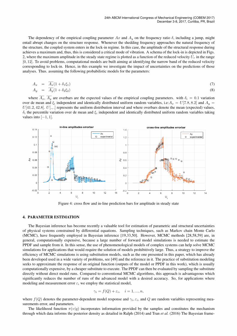
The dependency of the empirical coupling parameter Ax and Ay on the frequency ratio δ, including a jump, mightentail abrupt changes on the structure response. Whenever the shedding frequency approaches the natural frequency ofthe structure, the coupled system enters in the lock-in regime. In this case, the amplitude of the structural response duringachieves a maximum and, thus, this is considered a critical mode of vibration. A schema of the lock-in is depicted in Figs.2, where the maximum amplitude in the steady state regime is plotted as a function of the reduced velocity Ur in the range[0, 12]. To avoid problems, computational models are built aiming at identifying the narrow band of the reduced velocitycorresponding to lock-in. Hence, in this example we investigate the impact of uncertainties on the predictions of thoseanalyses. Thus. assuming the following probabilistic models for the parameters:

Ax = Ax(1 + δ1ξ1) (7)Ay = Ay(1 + δ2ξ2) (8)

where Ax, Ay are overbars are the expected values of the empirical coupling parameters. with δi = 0.1 variationover de mean and ξi independent and identically distributed uniform random variables, i.e:Ax = U [7.8, 8.2] and Ay =U [41.2, 42.8]. U [., .] represents the uniform distribution interval and where overbars denote the mean (expected) values,δi the percentile variation over de mean and ξi independent and identically distributed uniform random variables takingvalues into [−1, 1].

Figure 4: cross flow and in-line prediction bars for amplitude in steady state

4. PARAMETER ESTIMATION

The Bayesian inference has become recently a valuable tool for estimation of parametric and structural uncertaintiesof physical systems constrained by differential equations. Sampling techniques, such as Markov chain Monte Carlo(MCMC), have frequently employed in Bayesian inference [19,33,50]. However, MCMC methods [28,58,59] are, ingeneral, computationally expensive, because a large number of forward model simulations is needed to estimate thePPDF and sample from it. In this sense, the use of phenomenological models of complex systems can help solve MCMCsimulations for applications that would require the solution of models prohibitively large. Thus, a strategy to improve theefficiency of MCMC simulations is using substitution models, such as the one presented in this paper, which has alreadybeen developed used in a wide variety of problems, see [49] and the reference in it. The practice of substitution modelingseeks to approximate the response of an original function (outputs of the model or PPDF in this work), which is usuallycomputationally expensive, by a cheaper substitute to execute. The PPDF can then be evaluated by sampling the substitutedirectly without direct model runs. Compared to conventional MCMC algorithms, this approach is advantageous whichsignificantly reduces the number of runs of the advanced model with a desired accuracy. So, for applications wheremodeling and measurement error εi we employ the statistical model,

γi = f(Q) + εi, i = 1, ..., n,

where f(Q) denotes the parameter-dependent model response and γi, εi, and Q are random variables representing mea-surements error, and parameters.

The likelihood function π(υ|q) incorporates information provided by the samples and constitutes the mechanismthrough which data informs the posterior density as detailed in Ralph (2014) and Tran et al. (2016) The Bayesian frame-


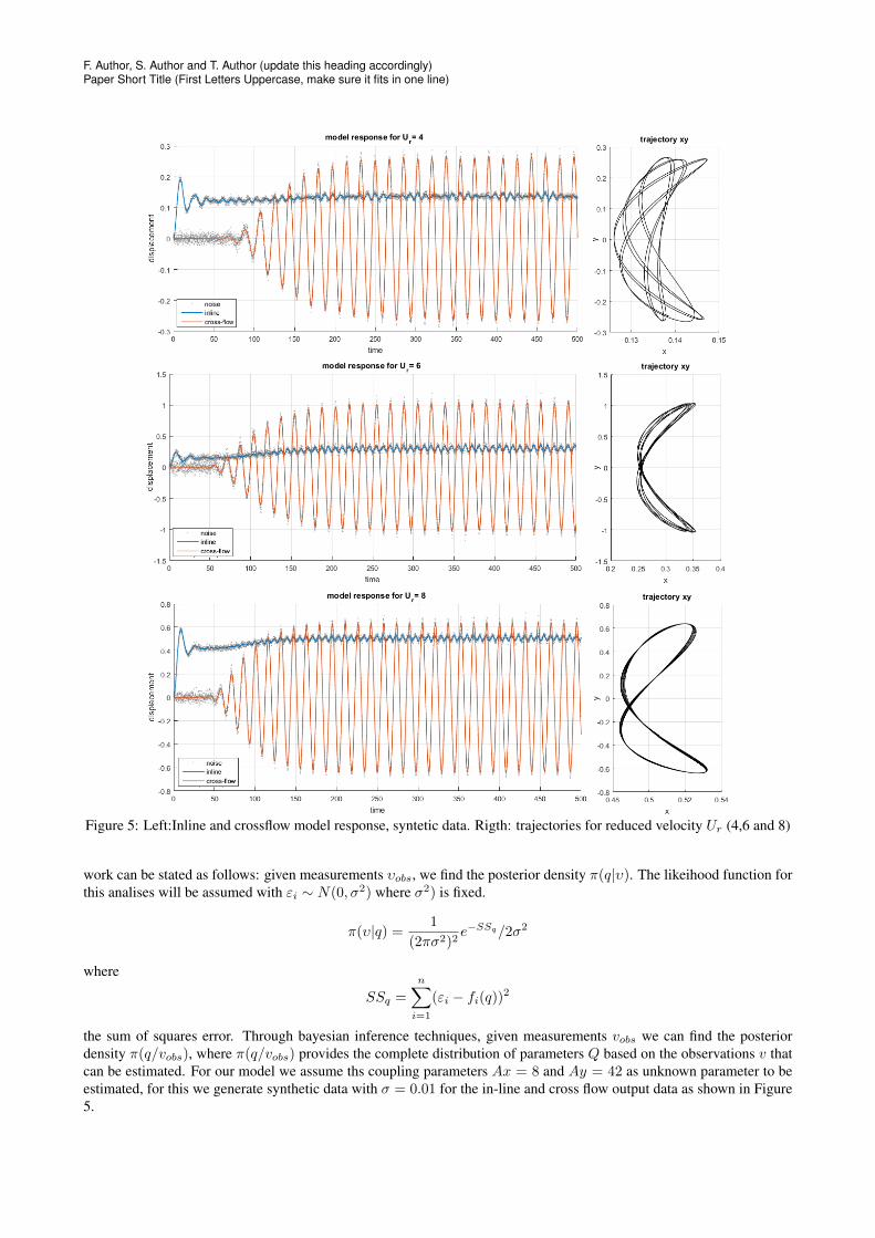
Figure 5: Left:Inline and crossflow model response, syntetic data. Rigth: trajectories for reduced velocity Ur (4,6 and 8)

work can be stated as follows: given measurements υobs, we find the posterior density π(q|υ). The likeihood function forthis analises will be assumed with εi ∼ N(0, σ2) where σ2) is fixed.

π(υ|q) =1

(2πσ2)2e−SSq/2σ2

where

SSq =

n∑i=1

(εi − fi(q))2

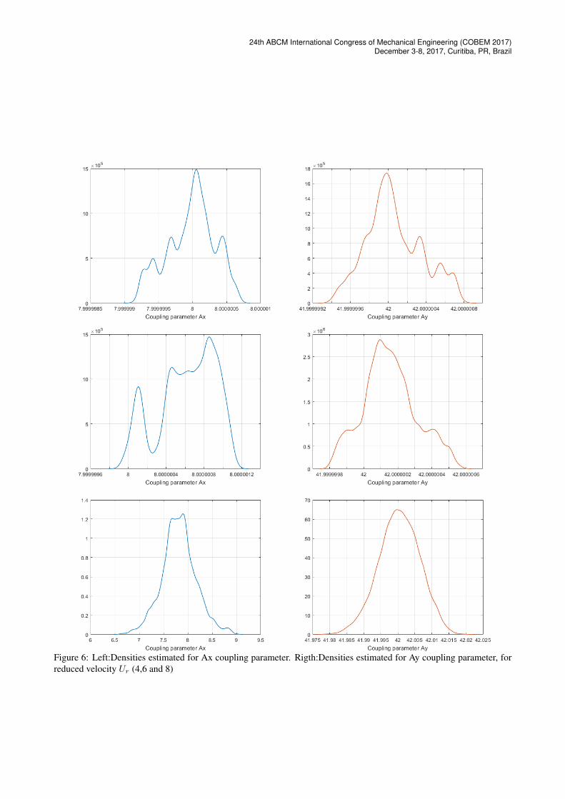
the sum of squares error. Through bayesian inference techniques, given measurements vobs we can find the posteriordensity π(q/vobs), where π(q/vobs) provides the complete distribution of parameters Q based on the observations v thatcan be estimated. For our model we assume ths coupling parameters Ax = 8 and Ay = 42 as unknown parameter to beestimated, for this we generate synthetic data with σ = 0.01 for the in-line and cross flow output data as shown in Figure5.


Figure 6: Left:Densities estimated for Ax coupling parameter. Rigth:Densities estimated for Ay coupling parameter, forreduced velocity Ur (4,6 and 8)


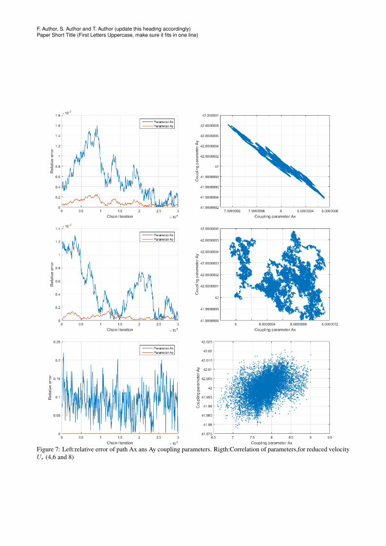
Figure 7: Left:relative error of path Ax ans Ay coupling parameters. Rigth:Correlation of parameters,for reduced velocityUr (4,6 and 8)


5. CONCLUSIONS

In this work, we have explored the capabilities sensitivity analyses and calibrations techniques using a subrrogatemodel that deals with the vibrational response of submerged structures excited by vortex detachments in the surroundingflow. We adopted a popular engineering model to predict this dynamics, with special attention to the lock-in phenomena.Two of the parameters used by this modeling were considered uncertain, inasmuch as they often are obtained by meansof model calibration based on field observations or physical experiments. An Adaptive Sparse Grid Collocation Methodwas used to estimate the statistical moments. This non-intrusive method, allow convert any deterministic code into acode that solves the corresponding stochastic problem. Compared with the Monte Carlo Simulation method, the ASGCmethod presents a significative reduction in the number of experiments required to achieve the same level of accuracy.The results obtained, show that it is possible refine the grid locally identifying automatically non smooth regions in thestochastic space achieving the same accuracy and reducing significatively the cost by the use of less collocations pointsin smooth regions of the stochastic space. Due to that the majority of engineering problems varying rapidly in only somedimensions, remaining much smoother in other dimensions and in general it have more stochastic dimensions.After thisanalyses we try calibrate two coupling parameter of parameters in the surrogate model using Bayesian technique. Theresults obtained are preliminary and need to be analyzed deeper. Future work will include analysis of sensitivity for othersparameters as well the use of experimental data to validate and calibrate the models.

6. ACKNOWLEDGEMENTS

This optional section must be placed before the list of references.

7. REFERENCES

Babuska, I., Tempone, R. and Zouraris, G.E., 2004. “Galerkin finite element approximations of stochastic elliptic partialdifferential equations”. SIAM Journal on Numerical Analysis, Vol. 42, No. 2, pp. 800–825.

Elishakoff, I., 2003. “Notes on philosophy of the monte carlo method”. International Applied Mechanics, Vol. 39, pp.753–762 10.

Facchinetti, M.L., de Langre, E. and Biolley, F., 2004. “Coupling of structure and wake oscillators in vortex-inducedvibrations”. Journal of Fluids and Structures, Vol. 19, No. 2, pp. 123 – 140. ISSN 0889-9746.

Gabbai, R. and Benaroya, H., 2005. “An overview of modeling and experiments of vortex-induced vibration of circularcylinders”. Journal of Sound and Vibration, Vol. 282, No. 3-5, pp. 575 – 616. ISSN 0022-460X.

Kreuzer, E., 2008. IUTAM Symposium on Fluid-Structure Interaction in Ocean Engineering: Proceedings of the IUTAMSymposium held in Hamburg, Germany, July 23-26, 2007. Iutam Bookseries. Springer. ISBN 9781402086298.

Ma, X. and Zabaras, N., 2009. “An adaptive hierarchical sparse grid collocation algorithm for the solution of stochasticdifferential equations”. Journal of Computational Physics, Vol. 228, pp. 3084–3113. ISSN 0021-9991.

Postnikov, A., Pavlovskaia, E. and Wiercigroch, M., 2017. “2dof cfd calibrated wake oscillator model to investigatevortex-induced vibrations”. International Journal of Mechanical Sciences, Vol. 127, No. Supplement C, pp. 176 –190. ISSN 0020-7403. Special Issue from International Conference on Engineering Vibration - ICoEV 2015.

Ralph, S., 2014. Uncertinty Quantification, Theory, Implementation, and Aplications. SIAM, 3rd edition. ISBN0321193687.

Rosetti, G.F., Goncalves, R.T., Fujarra, A.L.C. and Nishimoto, K., 2011. “Parametric analysis of a phenomenologicalmodel for vortex-induced motions of monocolumn platforms”. Journal of the Brazilian Society of Mechanical Sciencesand Engineering, Vol. 33, pp. 139 – 146. ISSN 1678-5878.

Toyanov, M.S., 2016. “User manual: Tasmanian sparse grid”. ORNL Technical Report, Vol. 1, No. 1.Tran, H., Webster, C.G. and Zhang, G., 2016. A Sparse Grid Method for Bayesian Uncertainty Quantification with

Application to Large Eddy Simulation Turbulence Models, Springer International Publishing, Cham, pp. 291–313.Xiu, D. and Hesthaven, J.S., 2005. “High-order collocation methods for differential equations with random inputs”. SIAM

Journal on Scientific Computing, Vol. 27, No. 3, pp. 1118–1139.Xiu, D., Lucor, D., Su, C.H. and Karniadakis, G.E., 2002. “Stochastic modeling of flow-structure interactions using

generalized polynomial chaos”. Journal of Fluids Engineering, Vol. 124, No. 1, pp. 51–59.

8. RESPONSIBILITY NOTICE

The following text, properly adapted to the number of authors, must be included in the last section of the paper: Theauthor(s) is (are) the only responsible for the printed material included in this paper.

Documents

Statistical calibration of 2DOF vortex-induced vibration