Embed Size (px)
Citation preview
Vortex Induced Vibration Energy Harvesting through Piezoelectric Transducers
A Major Qualifying Project
Submitted to the Faculty of the
WORCESTER POLYTECHNIC INSTITUTE
In partial fulfillment of the requirements for the
Degree of Bachelor of Science
Submitted By:
Natalie Diltz
Julie Gagnon
Jacqueline O’Connor
Jessica Wedell
Project Advisor:
Professor Brian J. Savilonis
Submitted:
4/20/2017
1
Abstract
Harvesting energy from vortex induced vibrations (VIV) in flowing water has the
potential to be a low-impact, low-cost alternative to traditional hydropower methods. This
project focused on utilizing piezoelectric transducers to transform the VIV oscillations of a
cylinder to electrical power. Initial prototypes focused on achieving these oscillations. The final
prototype of this stage produced an average amplitude of 12mm and frequency of 3.2 Hz. These
values were used to determine the design of the piezoelectric system. The second stage of
prototyping focused on generating power through the integration of the existing prototype and
the piezoelectric transducers. The final prototype successfully produced up to 0.1 microwatts,
but the erratic flow speed of the testing facilities and the project’s small scale prevented
consistent power generation. The project concluded that additional experimentation needs to be
conducted on a larger scale in order to determine the real world feasibility of VIV piezoelectric
energy harvesting.
2
Table of Contents
Abstract .......................................................................................................................................... 1
Table of Contents ........................................................................................................................... 2
List of Figures ................................................................................................................................ 4
List of Tables ................................................................................................................................. 5
1. Introduction ................................................................................................................................ 6
2. Background ................................................................................................................................ 8
2.1 VIV Theory .......................................................................................................................... 8
2.1.1 Vortex Shedding ........................................................................................................... 8
2.1.2 Vortex Induced Vibration ........................................................................................... 11
2.1.3 Important Parameters .................................................................................................. 11
2.1.4 Synchronization .......................................................................................................... 14
2.1.5 Harmonic Model of VIV ............................................................................................ 15
2.2 Applications ....................................................................................................................... 17
2.2.1. Environmental Factors ............................................................................................... 18
2.2.2. Cost ............................................................................................................................ 19
2.3 Past Research ..................................................................................................................... 19
2.3.1 Past MQPs .................................................................................................................. 19
2.3.2 VIVACE ..................................................................................................................... 20
2.3.3 Areas of Interest .......................................................................................................... 21
2.4 Energy Harvesting and Measurement ................................................................................ 22
2.4.1 Mechanical Energy ..................................................................................................... 22
2.4.2 Electromagnetic Harvesting System ........................................................................... 23
2.4.3 Electrostatic ................................................................................................................ 25
2.4.4 Piezoelectric ................................................................................................................ 26
2.4.5 Maximum Power Output ............................................................................................ 28
3. Piezoelectric Testing and Prototyping .................................................................................... 32
3.1 Piezoelectric Transducer Testing ....................................................................................... 32
3.1.1 Measurement Methods ................................................................................................ 33
3.1.2 Full Bridge Rectifier ................................................................................................... 33
3.1.3 Ceramic Disc Piezoelectric ......................................................................................... 34
3.1.4 Film Piezoelectric ....................................................................................................... 35
3.1.5 Power Output .............................................................................................................. 36

3
3.1.6 Circuit Components .................................................................................................... 36
3.2 Oscillator Constraints and Design ..................................................................................... 37
3.2.1 Testing Location ......................................................................................................... 37
3.2.2 Oscillator Design ........................................................................................................ 39
3.3 Testing Procedures for Oscillator Prototypes .................................................................... 44
3.3.1 Flowing Water Tests ................................................................................................... 44
3.3.2 Still Water Tests ......................................................................................................... 45
3.4 Oscillator Prototypes ......................................................................................................... 46
3.4.1 Prototype #1: Drawer Sliders Design ......................................................................... 46
3.4.2 Prototype #2: Sleeve-bearing Guide Rail Design ....................................................... 47
3.4.3 Prototype #3: Freely Suspended Cylinder Design ...................................................... 48
3.4.4 Prototype #4: Slot Design ........................................................................................... 50
4. Methodology ............................................................................................................................ 55
4.1 Energy Harvester Design ................................................................................................... 55
4.2 Flowing Water Testing Procedure ..................................................................................... 56
4.3 Optimal Load Testing Procedure ....................................................................................... 57
5. Results...................................................................................................................................... 59
5.1 Rowing Tank Water Velocity ............................................................................................ 59
5.2 Energy Harvester Power Output ........................................................................................ 62
5.2.1 Voltage and Power Output.......................................................................................... 62
5.2.2 Efficiencies ................................................................................................................. 63
5.3 Resistance Testing ............................................................................................................. 64
6. Conclusions and Recommendations ........................................................................................ 66
6.1 Oscillations ........................................................................................................................ 66
6.2 Power Generation .............................................................................................................. 66
6.3 Efficiency ........................................................................................................................... 66
6.4 Intermittent Oscillations .................................................................................................... 67
6.5 Recommendations for Future Testing (Small Scale) ......................................................... 68
6.6 Large Scale Testing and Real World Feasibility ............................................................... 69
References .................................................................................................................................... 71
Appendix A: Materials List ......................................................................................................... 75
4
List of Figures
Figure 1: A Von Kármán Vortex Street ......................................................................................... 9
Figure 2: Reynolds Number Regimes for Fluid Flow across Smooth Cylinders ........................ 10
Figure 3: Graph Showing the Relationship between the Strouhal and Reynolds Numbers ........ 12
Figure 4: Synchronization Range of a Cylinder as a Function of m* and U* ............................ 15
Figure 5: Overview of the VIVACE Converter ........................................................................... 21
Figure 6: Prony Brake Dynamometer .......................................................................................... 23
Figure 7: A Theoretical Electromagnetic Set-Up ........................................................................ 24
Figure 8: VIVACE Energy Converter Senior Project ................................................................. 25
Figure 9: Mechanical Stresses on Piezo Elements ...................................................................... 27
Figure 10: Rectifying Circuit for a Piezoelectric Harvester ........................................................ 27
Figure 11: Demonstrates the Maximum Power Output Possible for a Given Resistive Load ..... 29
Figure 12: Mechanical System Decision Matrix ......................................................................... 30
Figure 13: Electrical System Decision Matrix ............................................................................. 30
Figure 14: Rectifier Circuit Diagram ........................................................................................... 33
Figure 15: Rectifier Circuit Input and Output Waveforms .......................................................... 34
Figure 16: Model of the Film Piezoelectric Voltage Source ....................................................... 35
Figure 17: Layout of Rowing Tanks ............................................................................................ 37
Figure 18: Rowing Tank Bottom-to-ledge Height ....................................................................... 38
Figure 19: Rowing Tank Width ................................................................................................... 39
Figure 20: Tank Rig Set Up ......................................................................................................... 40
Figure 21: Oscillator Frame and Tank Rig .................................................................................. 42
Figure 22: Oscillator Frame ......................................................................................................... 43
Figure 23: Drawer Sliders ............................................................................................................ 46
Figure 24: Sleeve-bearing guide rail from McMaster-Carr ......................................................... 48
Figure 25: Sleeve-bearing carriage from McMaster-Carr ........................................................... 48
Figure 26: Oscillation Height vs. Time, Rowing Tank, 605 speed ............................................. 49
Figure 27: Oscillation Height vs. Time, Still Water Test ............................................................ 50
Figure 28: Slot Design ................................................................................................................. 52
Figure 29: Connection of Piezoelectrics to the Oscillator ........................................................... 56
Figure 30: Energy Harvester Testing Setup ................................................................................. 57
Figure 31: Water Velocities at Rowing Tank Settings ................................................................ 59
Figure 32: Average Measured Velocity vs Tank Control Speed ................................................. 60
Figure 33: Velocity Range at Different Tank Speed Settings ..................................................... 60
Figure 34: Water Velocity over Time at a Constant Tank Setting .............................................. 61
Figure 35: Voltage and Water Velocity ....................................................................................... 63
Figure 36: Power Output vs Load Resistance .............................................................................. 64
Figure 37: Simulated Rowing Tank Water Velocity Profile ....................................................... 68

5
List of Tables
Table 1: Voltage Output at Increasing Capacitance .................................................................... 36 Table 2: Voltage Output at Increasing Resistance ....................................................................... 37 Table 3: Rowing Tank Dimensions ............................................................................................. 38 Table 4: Parameters Used for Amplitude and Power Estimation ................................................ 40 Table 5: Still Water Testing Results for Prototype #1 ................................................................. 47
Table 6: Flowing Water Results for Prototype #3 ....................................................................... 49 Table 7: Still Water Testing Results for Prototype 3 ................................................................... 50 Table 8: Flowing Water Results for Slot Design Prototype ........................................................ 53 Table 9: Predicted and Measured Amplitude and Frequency ...................................................... 53 Table 10: Power Output ............................................................................................................... 62
6
1. Introduction
The production of clean, renewable energy is one of the biggest challenges faced by the
world today. Currently, the United States generates approximately 90% of its energy from
nonrenewable sources such as coal, natural gas, and oil. These resources are being drained at an
unsustainable rate and are the leading contributors to environmental problems such as pollution
and global warming. In recent decades, geothermal, wind, solar, biomass, and hydropower have
been explored as renewable energy sources. However, these energy sources still only make up
about 10% of US energy consumption because they are more expensive and require larger
amounts of land than their non-renewable counterparts (US Energy Information
Administration).
Currently, hydropower accounts for 46% of renewable energy in the US. Hydropower is
a particularly promising field because rivers and oceans make up about 71% of Earth’s surface
area. In spite of that promise, many of the current methods of harnessing hydropower energy
have significant drawbacks. Hydropower dams are the most commonly used method due to the
amount of power they can produce. However, they can only be built on large rivers with large
flow rates, which limits accessibility to this type of power. Additionally, dams can have
significant negative impacts on river ecosystems and wildlife. Other common methods of
hydropower production include wave generators and underwater turbines. While these methods
have potential, wave generators are limited in location because they disrupt surface marine
transit and turbines are limited to rivers with a current of at least 2 m/s.
A new type of hydropower energy harvests the power of vortex induced vibrations
(VIV). VIV is a phenomenon that occurs when a bluff body is placed in a flowing fluid; a shear
layer forms on either side of the body, and as the shear layers separate, they curl back behind
the body forming a pattern of alternating vortices. These vortices exert an oscillatory lift force
on the body, causing it to vibrate up and down. These vibrations can then be harvested as
electrical power. VIV has several advantages over other hydropower methods. For one, VIV can
be used in flow speeds ranging from 0.2 to 2.5 m/s. This versatility means that VIV has the
potential to be used in low current applications and along coastlines. In addition, VIV devices
are more environmentally friendly because they cause minimal damage or alterations to
ecosystems and do not interrupt marine traffic.
7
While VIV has many benefits, it is currently not commercially utilized as a form of
power generation. One of the main challenges of utilizing VIV is determining how to maximize
the power that can be harvested from the oscillations. Significant research has been done on
how to maximize the amplitude and frequency of the vibrations. Previous MQPs investigated
changing the size, material, and dimensions of the oscillating body. However, there is still need
for further research into how to effectively use VIV to generate power.
The goal of this project was to construct a VIV energy harvester that converts the
oscillations of a cylinder into electrical power through the use of piezoelectric transducers. The
harvester was tested in flowing water and optimal electrical load resistance testing was
conducted outside the water. The VIV harvester was able to produce 0.1µW of power in the
flowing water. However, continuous oscillation proved difficult because of inconsistent flow
speed of the testing location. It was concluded that additional testing needs to be conducted in
order to ascertain the viability of piezoelectric VIV energy harvesting.
8
2. Background
The purpose of this chapter is to introduce vortex induced vibrations, its applications,
past research, and methods of energy harvesting. The following section describes the theory
behind vortex shedding and vortex induced vibrations as well as some of the parameters and
equations that can be used to characterize it. Section 2.2 discusses some of the benefits and
applications of VIV, particularly as it relates to energy harvesting. Section 2.3 presents some of
the previous research that has been done in this field, including past MQPs at WPI and the
VIVACE converter developed at the University of Michigan. Finally, Section 2.4 examines
different methods of energy harvesting and energy conversion. This section also discusses the
theory behind maximizing power through changing the load on a device.
2.1 VIV Theory
2.1.1 Vortex Shedding
Vortex shedding is a phenomenon that occurs as the result of a viscous fluid flowing
over a bluff body, such as a cylinder, which causes a boundary layer to form due to the shear
viscosity of the fluid. As the fluid flows over the bluff body, the boundary layers separate and
form two separate shear layers trailing behind the body (Bearman, 196). The fluid closer to the
body, which is in contact with the wake, moves slower than the fluid near the outer edges of the
shear layer, which is in contact with the free stream. As a result, in the near wake of the body,
the fluid rotates inwards, forming distinct vortices that are shed from the body and travel down
the wake (Blevins, 45).
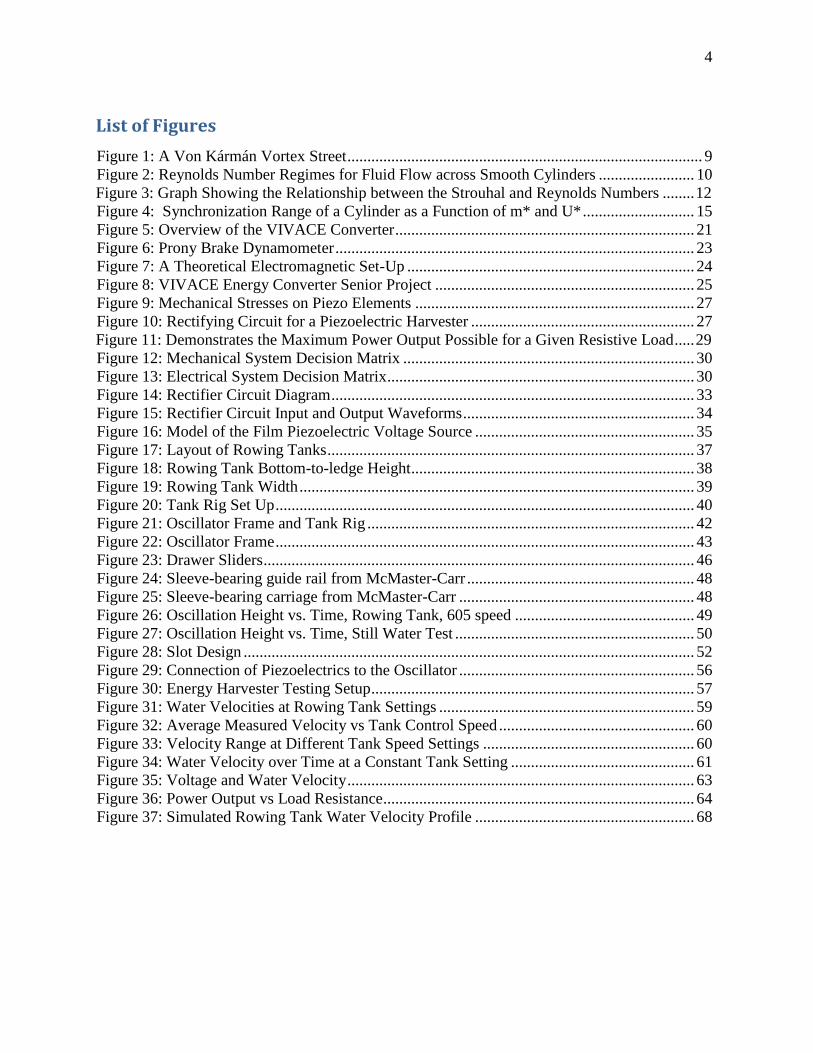
The vortices on each side of the bluff body are opposite in sign and will form a regular
periodic pattern in the wake known as a vortex street. The formation of a vortex street was
examined by Theodore von Kármán, who developed a model for an ideal vortex street (Figure
1). He found that the ideal spacing for a vortex street was h/ l =0.281, where h is the vertical
distance between vortices, and l is the horizontal distance between vortices (Blevins, 46).
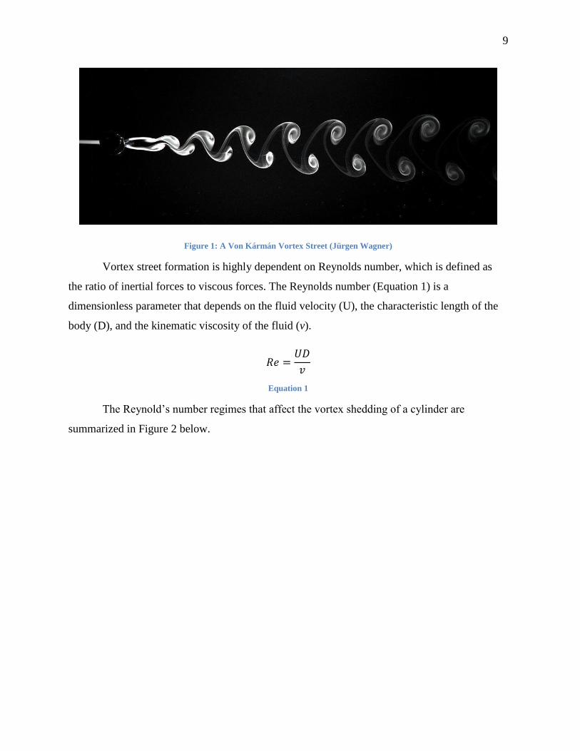
9
Figure 1: A Von Kármán Vortex Street (Jürgen Wagner)
Vortex street formation is highly dependent on Reynolds number, which is defined as
the ratio of inertial forces to viscous forces. The Reynolds number (Equation 1) is a
dimensionless parameter that depends on the fluid velocity (U), the characteristic length of the
body (D), and the kinematic viscosity of the fluid (v).
𝑅𝑒 =𝑈𝐷
𝑣
Equation 1
The Reynold’s number regimes that affect the vortex shedding of a cylinder are
summarized in Figure 2 below.
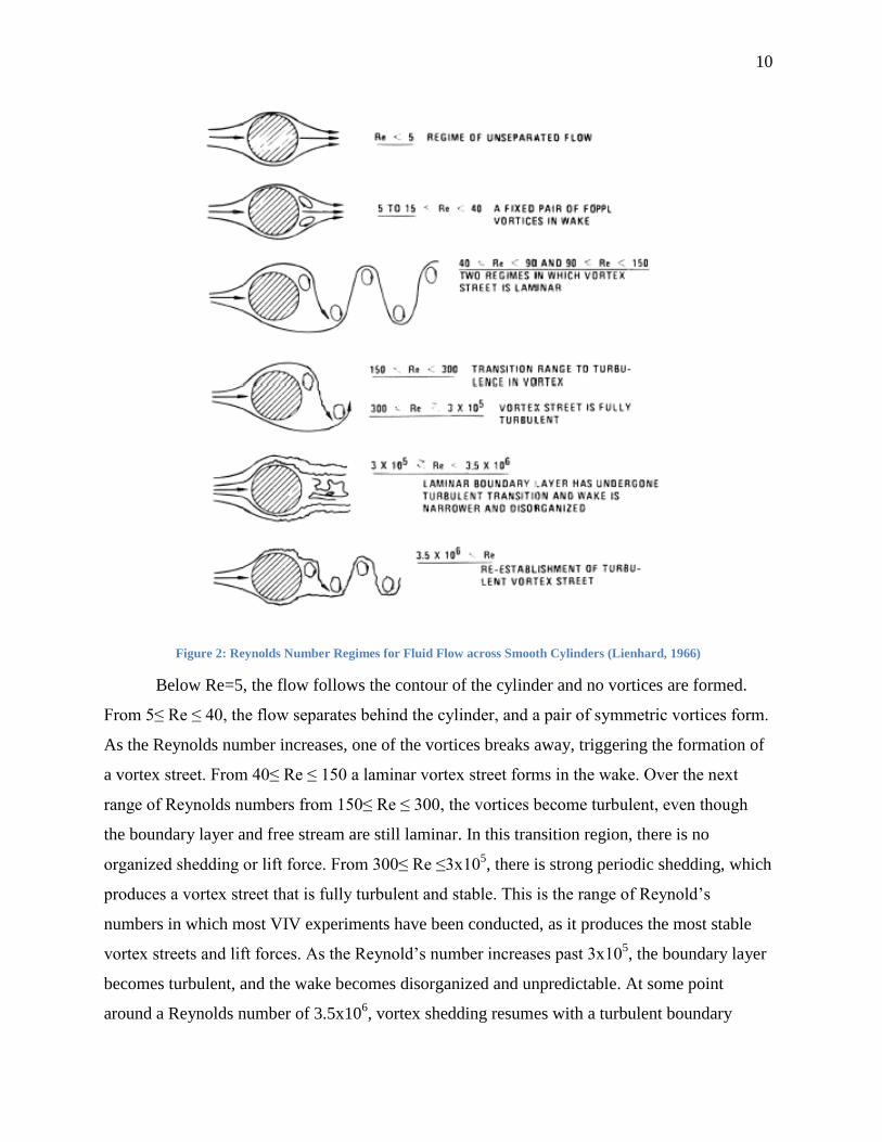
10
Figure 2: Reynolds Number Regimes for Fluid Flow across Smooth Cylinders (Lienhard, 1966)
Below Re=5, the flow follows the contour of the cylinder and no vortices are formed.
From 5≤ Re ≤ 40, the flow separates behind the cylinder, and a pair of symmetric vortices form.
As the Reynolds number increases, one of the vortices breaks away, triggering the formation of
a vortex street. From 40≤ Re ≤ 150 a laminar vortex street forms in the wake. Over the next
range of Reynolds numbers from 150≤ Re ≤ 300, the vortices become turbulent, even though
the boundary layer and free stream are still laminar. In this transition region, there is no
organized shedding or lift force. From 300≤ Re ≤3x10⁵, there is strong periodic shedding, which
produces a vortex street that is fully turbulent and stable. This is the range of Reynold’s
numbers in which most VIV experiments have been conducted, as it produces the most stable
vortex streets and lift forces. As the Reynold’s number increases past 3x10⁵, the boundary layer
becomes turbulent, and the wake becomes disorganized and unpredictable. At some point
around a Reynolds number of 3.5x10⁶, vortex shedding resumes with a turbulent boundary
11
layer. Vortex shedding has been observed at Reynolds numbers as high as 1011
, such as in wind-
driven cloud formations (Blevins, 46).
2.1.2 Vortex Induced Vibration
The vortices shed from bluff bodies exert oscillatory lift forces on the body due to
alternating pressures. If the body is flexible or unfixed, these forces will cause it to oscillate as
well (Benaroya & Gabbai). The oscillation of bluff bodies due to vortex shedding is known as
vortex induced vibration (VIV). While VIV can occur for any bluff body, this report will focus
on the vortex induced vibration of cylinders. The oscillations mostly occur in the direction
normal to the free stream, and cylinders can have oscillation amplitudes up to about twice the
size of the cylinder diameter (Bearman, 195).
2.1.3 Important Parameters
The vortex induced vibration of a cylinder is dependent on several key parameters. The
first important parameter is the Reynolds number. The Reynolds number, as discussed
previously, affects the vortex shedding pattern of the flow, meaning that VIV will only occur in
Reynolds regimes where there is a stable vortex street. For most VIV applications, this means
that Reynold’s number will be between 300 and 3x10⁵.
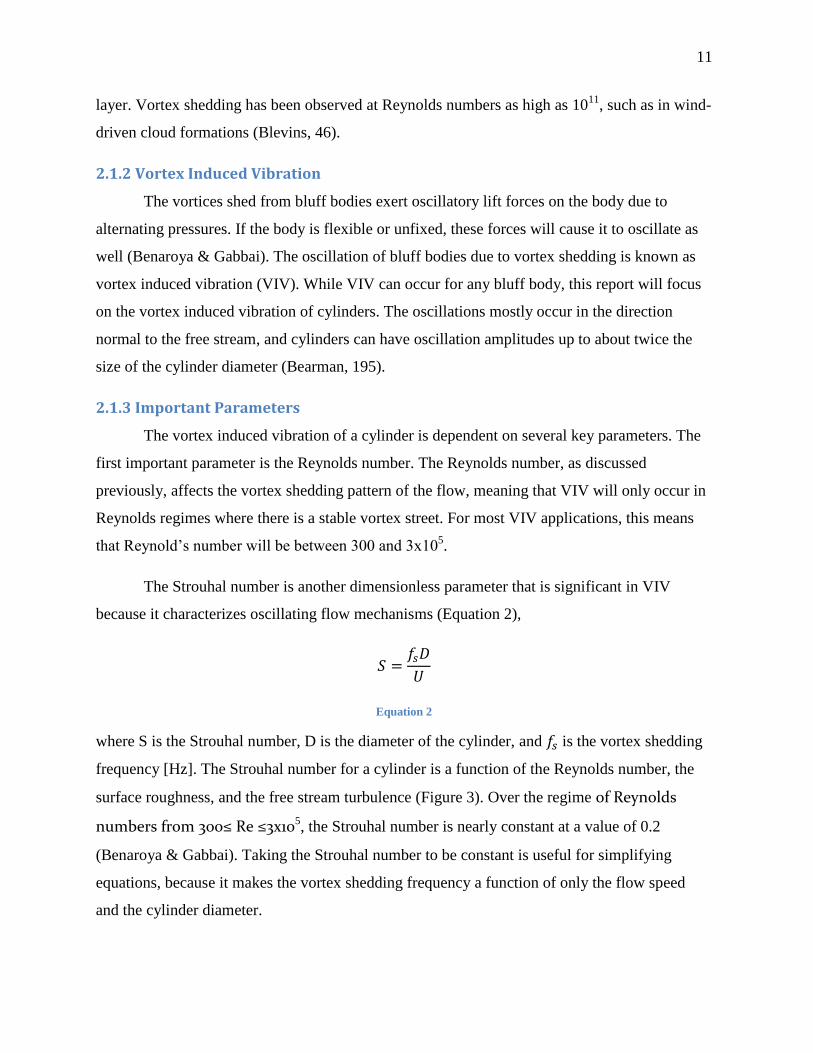
The Strouhal number is another dimensionless parameter that is significant in VIV
because it characterizes oscillating flow mechanisms (Equation 2),
𝑆 =𝑓𝑠𝐷
𝑈
Equation 2
where S is the Strouhal number, D is the diameter of the cylinder, and 𝑓𝑠 is the vortex shedding
frequency [Hz]. The Strouhal number for a cylinder is a function of the Reynolds number, the
surface roughness, and the free stream turbulence (Figure 3). Over the regime of Reynolds
numbers from 300≤ Re ≤3x10⁵, the Strouhal number is nearly constant at a value of 0.2
(Benaroya & Gabbai). Taking the Strouhal number to be constant is useful for simplifying
equations, because it makes the vortex shedding frequency a function of only the flow speed
and the cylinder diameter.
12
Figure 3: Graph Showing the Relationship between the Strouhal and Reynolds Numbers for a Cylinder (MIT)
A third parameter that affects vortex induced vibration is the mass ratio (m*). The mass
ratio is the ratio of the oscillator mass to the mass of the fluid it displaces (Equation 3).
𝑚∗ =𝑚𝑜𝑠𝑐
𝑚𝑑𝑖𝑠
Equation 3
𝑚𝑜𝑠𝑐 is the mass of the oscillating body plus ⅓ the total mass of the springs, and 𝑚𝑑𝑖𝑠 is the
mass of the fluid displaced by the cylinder. For a cylinder:
𝑚𝑑𝑖𝑠 = 𝜌𝜋
4𝐷2𝐿
Equation 4
D is the diameter of the cylinder, L is the length of the cylinder, and ρ is the density of the fluid.
Excluding the mass of the springs and any additional sources of mass attached to the cylinder,
the mass ratio reduces to the ratio between the density of the cylinder and the density of the
fluid (Modir, Kahrom, & Farshidianfar).
Two additional significant parameters of VIV are the structural damping factor or
damping ratio (ζ) and the aspect ratio of the cylinder (L/D). The damping factor is on a scale of
13
0 to 1, with one being the critical damping factor for the system. The critical damping is the
point at which the system of a damped oscillator goes from being underdamped to overdamped,
i.e. where the cylinder can no longer vibrate. The damping of a system is often characterized by
a dimensionless parameter called reduced damping, such as the Scruton number (Equation 5).
𝑆𝑐 =2𝑚(2𝜋𝜁)
𝜌𝐷2
Equation 5
D is the diameter of the cylinder, m is the mass of the cylinder per unit length, ρ is the density
of the fluid and ζ is the damping ratio. Increasing the reduced damping usually decreases the
amplitude of oscillations (Blevins, 9). Damping on the cylinder is the result of viscous forces,
which include the drag on the cylinder and the friction due to how the cylinder is mounted. The
drag force on the cylinder is not linear; it depends on the amplitude and reduced velocity of the
cylinder. Studies have attempted to model the damping ratio as a function of time. However,
most calculations assume an average value. The damping ratio for freely-suspended cylinders is
typically very low, on the scale of 0.06 or less. Any constraints on the cylinder where there is
friction will increase the damping on the system (Williamson & Govardhan, 2008). The average
damping for the system can be determined by performing a free decay test at a given starting
amplitude and measuring two consecutive amplitudes of the cylinder (Modir, Kahrom, &
Farshidianfar). The damping ratio is then calculated as follows, where yn is the first amplitude
and yn+1 is the second amplitude:
Equation 6
There are two more dimensionless parameters that are useful in characterizing the
oscillations of a system undergoing VIV. The first of these parameters is the reduced velocity
(U*) (Equation 7).
𝑈∗ =𝑈
𝑓𝑛𝐷
Equation 7

14
U is the fluid velocity, 𝑓𝑛 is the natural frequency of the system, and D is the diameter of the
cylinder. The final significant dimension parameter of VIV is the dimensionless amplitude,
which is defined as the ratio of the amplitude of the vibrations in the transverse direction to the
diameter of the cylinder (Blevins, 5).
2.1.4 Synchronization
A key feature of vortex induced vibration is the existence of a region of synchronization
or “lock-in.” In this region, there is a significant increase in the amplitude of the oscillations of
the cylinder, meaning that the energy of the system will be at a maximum. Synchronization is
similar to linear resonance, as it occurs when the vortex shedding frequency approaches the
natural frequency of the oscillator. However, unlike resonance, synchronization is nonlinear and
will occur over a band of frequencies. Additionally, synchronization does not have a sharp peak
in amplitude when the shedding frequency and the natural frequency are exactly equal. In the
lock-in region, the vibration of the cylinder controls the shedding frequency. Synchronization is
also described as being self-limiting, because when the amplitude grows too large the
symmetric pattern of vortices breaks up (Blevins, 54).
Most of the current understanding of lock-in is based on empirical or semi-empirical
studies; an analytical model of lock-in has not been fully developed. One of the most important
findings about the lock-in region is its dependence on the reduced velocity. Assuming a value of
0.2 for the Strouhal number, the reduced velocity, U*, is equal to 5 when the vortex shedding
frequency and the natural frequency are exactly equal. It has been experimentally determined
that synchronization will generally occur for 4< U* <8 (Blevins, 59).
While the reduced velocity is the best indicator of whether or not synchronization will
occur, it has also been found that the mass ratio affects the size of the lock-in region. For high
values of m*, the lock-in region is relatively constant between reduced velocities of 4 and 8. As
the mass ratio is decreased, the lock-in region becomes larger, until it reaches a critical point
where the lock-in band becomes infinitely large. Williamson and Govordhan found that this
critical mass ratio was equal to 0.54. This value was determined specifically for systems with a
low mass and low damping for an elastically supported cylinder. However, the existence of a
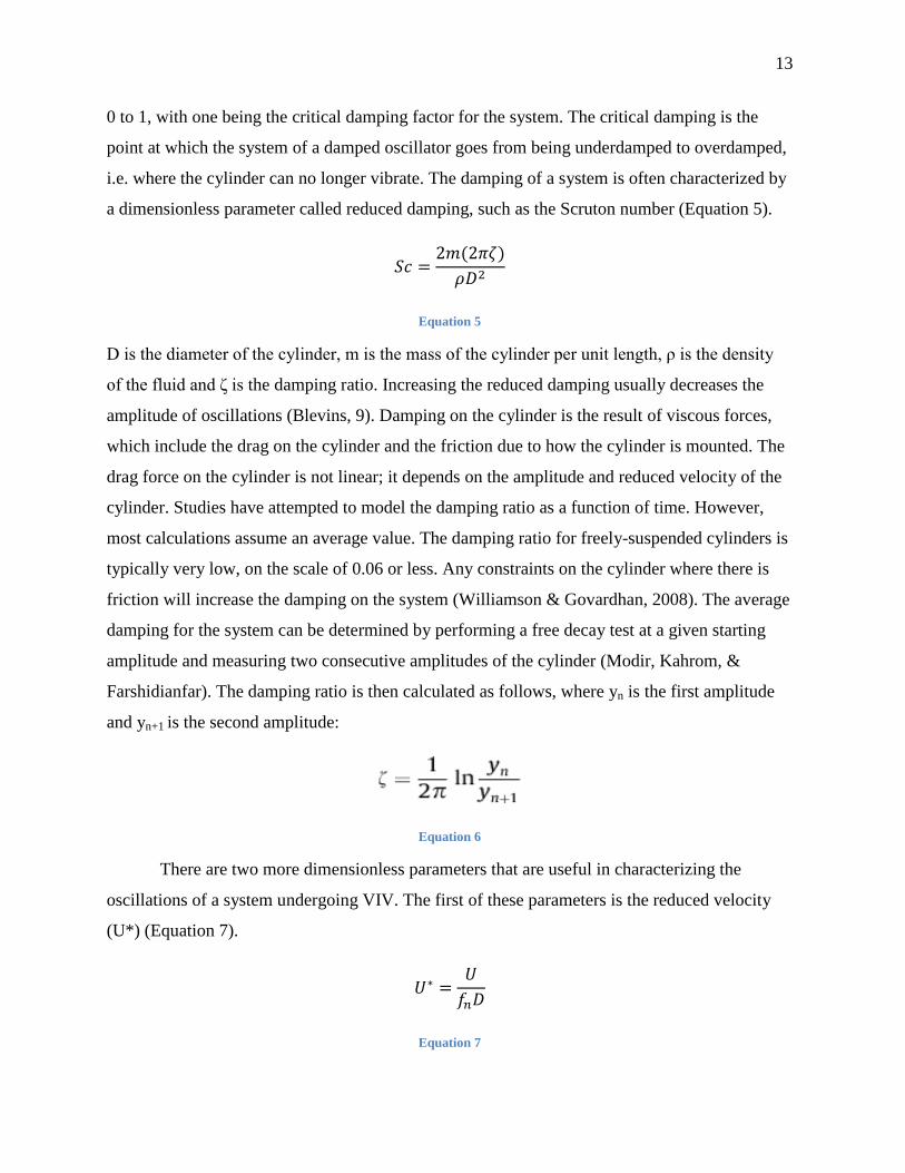
critical mass has been demonstrated for different geometries and damping factors. Figure 4
shows the synchronization range as it relates to both m* and U* for a cylinder. Lock-in will
15
occur within the shaded region.
Figure 4: Synchronization Range of a Cylinder as a Function of m* and U* (Williamson & Govordhan)
2.1.5 Harmonic Model of VIV
Due to the variable and non-linear nature of vortex induced vibrations, there is not one
set of governing equations to describe it. However, since vortex shedding is approximately
sinusoidal, VIV of a cylinder can be reasonably modeled as a linear harmonic oscillator
(Blevins, 61). The lift force exerted on the cylinder by the vortex shedding can therefore be
modeled as:
𝐹𝐿 =1
2𝜌𝑈2𝐷𝐿𝐶𝐿sin(𝜔𝑠𝑡)
Equation 8
FL is the lift force perpendicular to the free stream, ρ is the fluid density, U is the free stream
velocity, D is the cylinder diameter, L is the length of the cylinder, t is time [s], and ωs is the
angular vortex shedding frequency [rad/s], where𝜔𝑠 = 2𝜋𝑓𝑠. This force is applied to a cylinder
mounted elastically using springs of combined stiffness k. The motion of the cylinder can then
be described by Equation 9 below.
𝑚 + 2𝑚𝜁𝜔𝑛 + 𝑘𝑦 =1
2𝜌𝑈2𝐷𝐿𝐶𝐿sin(𝜔𝑠𝑡)
Equation 9
16
ωn is the angular natural frequency of the cylinder [rad/s], where 𝜔𝑛 = 2𝜋𝑓𝑛 = √𝑘(1−𝜁2
𝑚𝑜𝑐𝑠+𝑚𝑑𝑖𝑠, y is
the vertical displacement of the cylinder, with the apostrophes signifying differentiation with
respect to time, and 𝜁is the structural damping factor. For the linear oscillator model, the
damping factor is taken as an average and assumed to be constant. This differential equation can
be solved to produce an equation for the linear displacement of the cylinder with respect to
time, where 𝜑is the phase angle:
𝑦(𝑡) =
12𝜌𝑈
2𝐷𝐿𝐶𝐿sin(𝜔𝑠𝑡 + 𝜑)
𝑘√(1 − (𝜔𝑠
𝜔𝑛)2
)2 + (2𝜁𝜔𝑠
𝜔𝑛)2
Equation 10
From this equation, the amplitude at resonance can be found by setting𝜔𝑛 = 𝜔𝑠:
𝐴
𝐷=𝜔𝑛𝜌𝐿𝑈
2𝐶𝐿4𝑘𝜁
Equation 11
In reality the maximum amplitude will occur over a range of frequencies, not at exact
resonance. However, using the linear harmonic oscillator model provides a relatively accurate
approximation of the motion of a cylinder undergoing VIV.
The linear harmonic oscillator model of VIV also allows for the theoretical maximum
power to be calculated. The velocity as a function of time for the cylinder can be obtained by
differentiating Equation 10 for displacement, resulting in the following equation:
𝑣(𝑡) = −𝜔𝑠
12𝜌𝑈
2𝐷𝐿𝐶𝐿 cos(𝜔𝑠𝑡 + 𝜑)
𝑘√(1 − (𝜔𝑠
𝜔𝑛)2
)2 + (2𝜁𝜔𝑠
𝜔𝑛)2
Equation 12
Power as a function of time is found by multiplying the lift force and the cylinder velocity,
which gives:
17
𝑃(𝑡) = −𝜔𝑠
14𝜌
2𝑈4𝐷2𝐿2𝐶𝐿2𝑠𝑖𝑛(𝜔𝑠𝑡)𝑐𝑜𝑠(𝜔𝑠𝑡 + 𝜑)
𝑘√(1 − (𝜔𝑠
𝜔𝑛)2)2 + (2𝜁
𝜔𝑠
𝜔𝑛)2
Equation 13
The maximum power will occur when𝜔𝑛 = 𝜔𝑠. Given that for a cylinder𝜑 =𝜋
2, the equation
for the maximum power is given as:
𝑃𝑚𝑎𝑥 =𝜔𝑛𝜌
2𝑈4𝐷2𝐿2𝐶𝐿2 sin2(𝜔𝑛𝑡)
8𝑘𝜁
Equation 14
This equation estimates the system power of a cylinder undergoing VIV. As an example, for a
27.7 mm diameter PVC cylinder that is 229 mm long with a damping ratio of 0.1 suspended by
springs with a stiffness of 142.6 N/m in water flowing at 0.5 m/s, the maximum system power is
about 0.12 W. For a similar cylinder with a 63.5 mm diameter that is 305 mm long and in water
moving at 1m/s, the maximum power increases to 4.03W.
2.2 Applications
VIV is a viable energy source because it can be used in a multitude of environments.
VIV devices can be optimized in shape and size for low flow and low head water applications.
This ability makes it ideal for streams, small rivers, ocean currents and tidal waves which are
abundantly available yet underutilized because they are not dense enough for larger hydropower
capabilities. For example, the Gulf Stream moves at a maximum speed of 3 knots (Elert 2002),
while most hydropower harvesters require 5-6 knots to work efficiently. VIVACE, a VIV
harvesting device designed by University of Michigan engineers, is designed to generate power
in water flowing as slow as 2-4 knots. The VIVACE technology would make it possible to
harvest energy from the Gulf Stream as well as other river and ocean currents.
Vortex induced vibrations also occur at faster water velocities, making VIV harvesters a
highly adaptable energy source. Because of this adaptability, VIV could be used along
shorelines at sufficient depth. This is particularly beneficial because over 50% of the US
population lives within 50 miles of a coastline, which means there is a large demand for power
generation along the coast.
18
2.2.1. Environmental Factors
Vortex induced vibration devices have definitive advantages over other, more intrusive,
hydropower options. A dam, for example, changes the natural orientation of a river, harming
plants and wildlife both on land and in water. The most obvious illustration of this is the
obstruction of fish migration. While most modern dams are equipped with fish ladders
(underwater staircases that help fish navigate around obstacles) or other methods of fish
passage, these methods are not always effective and can cause declines in fish populations in
these areas (“American Shad”, University Communications, 2013).
Large hydropower dams create reservoirs that may flood areas where both humans and
wildlife inhabit, which would require relocation. An extreme illustration of this is the Three
Gorges Dam on the Yangtze River in China. When the dam was constructed, nearly 1.3 million
people were required to relocate since the reservoir would flood their villages (Kuhn, 2008). In
addition to these villages, approximately 2,000 archeological sites were also flooded. Some of
these sites dated back to the Paleolithic era and included ancient burial grounds (See, 2003).
Wave generators are much less harmful to the environment. Their underwater
infrastructure can actually create new habitats for smaller ocean organisms, though it may
obstruct larger ocean animals that could become entangled in the structure’s cables (OSU,
2015). Wave energy also restricts commercial fishing, creating a virtual marine reserve in their
installation area. The major negative side effect of wave generators is the interruption of ship
transportation. Due to their low profile and small size, wave generators are difficult to see on
the ocean’s surface and therefore create navigational hazards to vessels in the area where
generators are installed. Additionally, wave generators affect recreation and tourism due to their
visual impact and obstruction of activities such as watersports, swimming, and scuba diving
(“Environmental Impact of Wave Energy Devices”).
VIV devices can be located on the ocean or river floor; therefore they do not impede
shipping or recreational activities. Like wave generators, VIV devices would restrict fishing and
preserve marine life. However, VIV devices can be small in size and would not obstruct the
flow of a river or the transportation of fish. The environment both in and out of water around
these devices would remain relatively unchanged. For these reasons, VIV devices present an
environmental advantage over more popular, conventional hydropower options.
19
2.2.2. Cost
VIVACE engineers estimate that when the VIVACE system is deployed it will be able
to provide clean energy at 5.5 cents per kilowatt hour, which compares favorably to other forms
of clean energy. Wind energy, for example, costs 6.9 cents per kilowatt hour. Solar power can
cost anywhere from 16 to 48 cents per kilowatt hour (Flahiff 2008). While the cost of VIV
power is just an estimate because there are not currently any commercial projects, this estimate
suggests that VIV could be a competitive option in the renewable energy market.
2.3 Past Research
Due to the potential benefits of VIV for energy generation, there has been significant
research on utilizing it. Three previous MQPs at WPI have conducted research into VIV in
addition to the previously mentioned VIVACE at the University of Michigan.
2.3.1 Past MQPs
There have been three previous WPI MQP projects that experimented on topics of VIV.
They focused mainly on different ways to alter the geometry of the converter to maximize the
amplitude and frequency of the oscillations. However, none of these projects actually converted
VIV into usable power.
In 2011, Hall-Stinson, A. S., et al looked into testing various diameter sizes of the
cylinders to locate the correlation between diameter of the cylinder and different variables,
including oscillation frequency and mean amplitude. They conducted eighty-five tests with five
cylinders of different diameters for various criteria to determine the most ideal cylinder
diameter. Several masses were attached to each cylinder and suspended by springs from a fixed
point in the channel of their testing tank. The testing tank was an open flow channel with sump
pumps integrated to create a uniform and steady flow speed. With their tests, they determined
that a cylinder with a diameter of 1” (25.4 mm) produced the best results.
Also in 2011, Distler, D.B., et al experimented with the shape of the cross-sectional
body to see what would yield the largest displacement values. Using a typical cylinder as their
control group since it is the shape most commonly used in VIV experiments, the group digitally
experimented with a variety of additional shapes, such as triangles and ellipses, to determine the
optimal shape to build for testing. They concluded that the T-shape produced the largest lift
20
coefficient so it was chosen, along with a couple T-shaped variations, for their physical testing.
Similarly to Hall-Stinson, A. S., et al, Distler, D. B., et al constructed a tank with sump pumps
for their experiments. Their results were somewhat inconclusive, however, as they did not
determine whether the T-shape was more efficient than the control cylinder.
In 2012, Ball, I.M. et al continued the previous MQP’s research by attempting to
optimize the shape of the bluff object used. They also determined that the T-shape was the
optimal shape and built a tank to test that theory. The bluff objects being tested were attached to
a pivoting beam that was designed to have a specified natural frequency. They concluded that
the T-shape was the optimal shape and that the lock-in condition resulted in the greatest power
output.
2.3.2 VIVACE
As mentioned in Section 2.2.1, the group that has come the farthest in the pursuit of VIV
energy is Bernitsas, Raghavan, Ben-Simon and Garcia in their development of the Vortex
Induced Vibrations for Aquatic Clean Energy converter (VIVACE) at the University of
Michigan.
In their design, a cylinder is held aloft by two springs attached to end plates and
constrained so that it can freely vibrate up and down. The apparatus is attached to magnetic
sliders that travel along a rail containing a coil. When the system vibrates, the motion of the
magnets over the coil generates a DC current that can then be converted to AC and utilized for
power (Figure 5).

21
Figure 5: Overview of the VIVACE Converter (Vortex Hydro Energy)
In testing, the system was held stationary in a channel that produced water flow.
VIVACE engineers also acknowledged that similar testing results are possible by dragging the
apparatus through calm water at a constant velocity. Even at low speeds, VIV can transfer
kinetic energy into electricity, unlike more common forms of hydropower such as dams and
turbines. This is an advantage because it is a less invasive method of hydropower that can be
utilized in locations with less powerful streams. It has a low impact on the environment and can
be scaled up or down, depending on the need.
2.3.3 Areas of Interest
The three MQP groups and the VIVACE team have opened up many more avenues of
VIV experimentation and research through their studies.
Distler, D.B., et al recommended that the scale of the experimentation be increased.
They felt that it would “increase the validity of the data collected and may lead to more
conclusive paths to continue work” (Distler, D.B., et al). They also suggested experimenting
22
with various types of generators to determine the optimal power extraction method.
Hall-Stinson A.S., et al suggested that new tests with a higher fluid velocity/Reynolds
number be conducted in order to provide a more realistic condition to test the technology under.
They and Ball I. M. also suggested that future groups assess the possibility of conducting tests
in large-scale research laboratories such as the Alden Research Laboratory. These large-scale
labs have numerous tanks and other equipment designed to test various aspects of hydrokinetic
experimentation. Utilizing laboratories of this magnitude would result in cleaner data and less
time spent on the construction of a testing tank.
Based on the results and recommendations from the three WPI MQP groups and the
team at the University of Michigan, our team concluded that the next step in advancing VIV
research would be to construct an oscillator utilizing the findings of the previous MQPs and
actually convert the VIV into usable power.
2.4 Energy Harvesting and Measurement
In order to assess the VIV apparatus’ ability to harvest energy, it is important to
measure the power output of the overall system, potentially using dynamometers or linear force
sensors. VIV can also be converted into electrical power utilizing electromagnetic, piezoelectric
and electrostatic generators. The following sections will explore each of these options in detail.
2.4.1 Mechanical Energy
One type of energy harvesting is through the production of useful mechanical power that
can be used to drive a mechanical process. This often takes the form of a rotating shaft that can
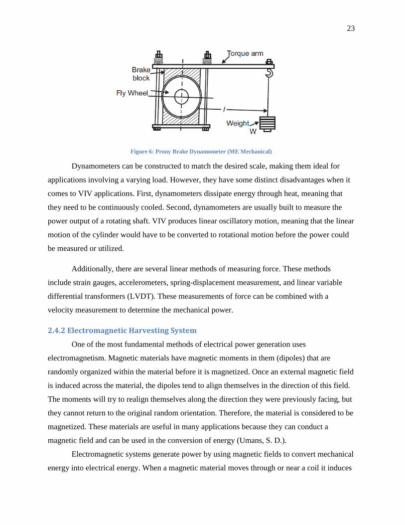
be used to drive rotational motion or converted into linear motion. A Dynamometer can be used
to measure the rotational mechanical power output. Absorption dynamometers are driven by the
motor or power source, and used to measure the power output, usually by measuring the torque
and the RPM of the rotating shaft. The load is varied by adding or removing weight to the lever
arm (Figure 6) (ME Mechanical).
23
Figure 6: Prony Brake Dynamometer (ME Mechanical)
Dynamometers can be constructed to match the desired scale, making them ideal for
applications involving a varying load. However, they have some distinct disadvantages when it
comes to VIV applications. First, dynamometers dissipate energy through heat, meaning that
they need to be continuously cooled. Second, dynamometers are usually built to measure the
power output of a rotating shaft. VIV produces linear oscillatory motion, meaning that the linear
motion of the cylinder would have to be converted to rotational motion before the power could
be measured or utilized.
Additionally, there are several linear methods of measuring force. These methods
include strain gauges, accelerometers, spring-displacement measurement, and linear variable
differential transformers (LVDT). These measurements of force can be combined with a
velocity measurement to determine the mechanical power.
2.4.2 Electromagnetic Harvesting System
One of the most fundamental methods of electrical power generation uses
electromagnetism. Magnetic materials have magnetic moments in them (dipoles) that are
randomly organized within the material before it is magnetized. Once an external magnetic field
is induced across the material, the dipoles tend to align themselves in the direction of this field.
The moments will try to realign themselves along the direction they were previously facing, but
they cannot return to the original random orientation. Therefore, the material is considered to be
magnetized. These materials are useful in many applications because they can conduct a
magnetic field and can be used in the conversion of energy (Umans, S. D.).
Electromagnetic systems generate power by using magnetic fields to convert mechanical
energy into electrical energy. When a magnetic material moves through or near a coil it induces
24
a force on the coil. The resulting force changes the magnetic field, inducing an electromotive
force (Equation 15). The amount of electromotive force directly relates to the amount of current
that is induced across the circuit through the following equation,
𝐸𝑚𝑓 = 𝑁 ∗ 𝑖
Equation 15
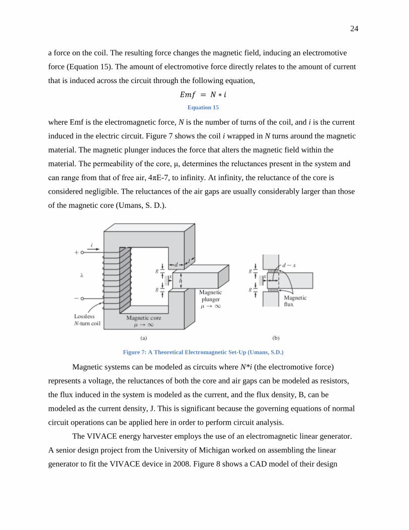
where Emf is the electromagnetic force, N is the number of turns of the coil, and i is the current
induced in the electric circuit. Figure 7 shows the coil i wrapped in N turns around the magnetic
material. The magnetic plunger induces the force that alters the magnetic field within the
material. The permeability of the core, μ, determines the reluctances present in the system and
can range from that of free air, 4πE-7, to infinity. At infinity, the reluctance of the core is
considered negligible. The reluctances of the air gaps are usually considerably larger than those
of the magnetic core (Umans, S. D.).
Figure 7: A Theoretical Electromagnetic Set-Up (Umans, S.D.)
Magnetic systems can be modeled as circuits where N*i (the electromotive force)
represents a voltage, the reluctances of both the core and air gaps can be modeled as resistors,
the flux induced in the system is modeled as the current, and the flux density, B, can be
modeled as the current density, J. This is significant because the governing equations of normal
circuit operations can be applied here in order to perform circuit analysis.
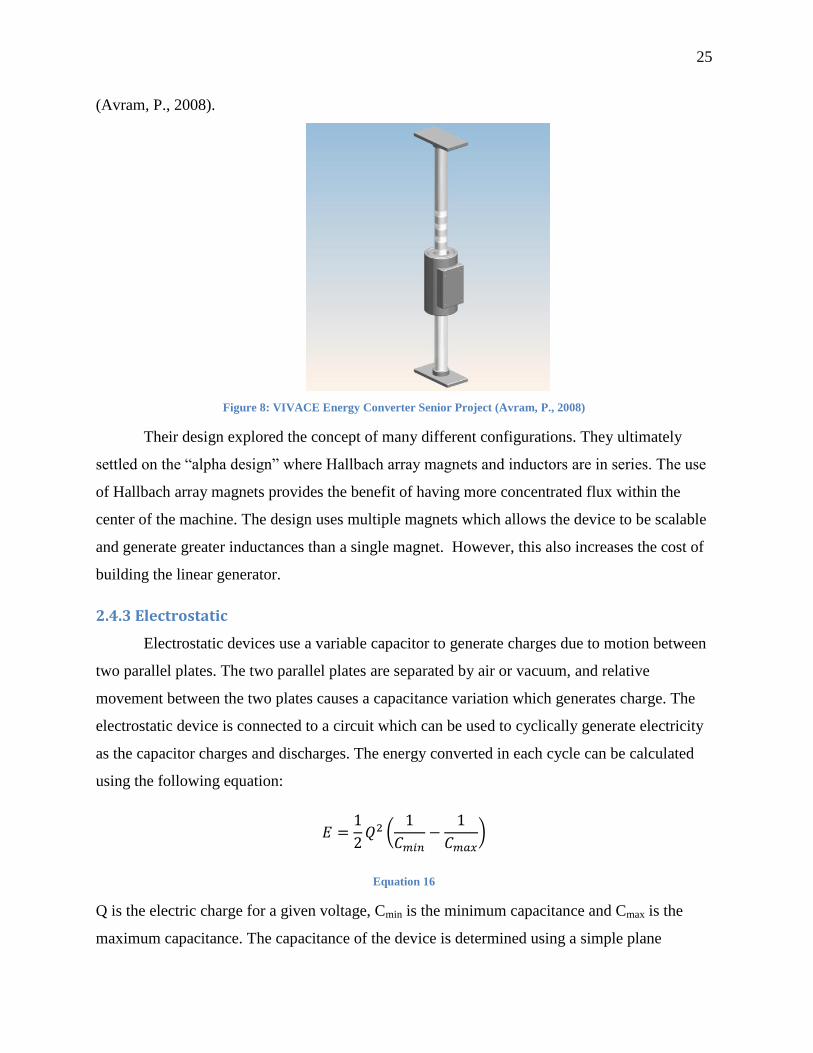
The VIVACE energy harvester employs the use of an electromagnetic linear generator.
A senior design project from the University of Michigan worked on assembling the linear
generator to fit the VIVACE device in 2008. Figure 8 shows a CAD model of their design
25
(Avram, P., 2008).
Figure 8: VIVACE Energy Converter Senior Project (Avram, P., 2008)
Their design explored the concept of many different configurations. They ultimately
settled on the “alpha design” where Hallbach array magnets and inductors are in series. The use
of Hallbach array magnets provides the benefit of having more concentrated flux within the
center of the machine. The design uses multiple magnets which allows the device to be scalable
and generate greater inductances than a single magnet. However, this also increases the cost of
building the linear generator.
2.4.3 Electrostatic
Electrostatic devices use a variable capacitor to generate charges due to motion between
two parallel plates. The two parallel plates are separated by air or vacuum, and relative
movement between the two plates causes a capacitance variation which generates charge. The
electrostatic device is connected to a circuit which can be used to cyclically generate electricity
as the capacitor charges and discharges. The energy converted in each cycle can be calculated
using the following equation:
𝐸 =1
2𝑄2 (
1
𝐶𝑚𝑖𝑛−
1
𝐶𝑚𝑎𝑥)
Equation 16
Q is the electric charge for a given voltage, Cmin is the minimum capacitance and Cmax is the
maximum capacitance. The capacitance of the device is determined using a simple plane
26
capacitance model. Electrostatic devices can be used for vibrational energy harvesting, utilizing
the vibration of the cylinder as the two plates move relative to each other (Boisseau, Despesse,
& Seddik).
2.4.4 Piezoelectric
Piezoelectric materials have a unique ability to convert mechanical stresses into
electrical energy. These materials have crystalline structures and generally contain electric
dipoles. When a mechanical stress is applied, it changes the direction of polarization and
produces an electrical field (Ledoux, 2011). The amount of voltage that is generated is directly
proportional to the stress on the chosen material. Piezoelectricity is useful in small applications
because of its small size and broad range of operating frequencies.
Piezoelectricity depends on a combination of the linear electrical behavior of a material
(Equation 17) and Hooke’s law for linear elastic materials (Equation 18).
𝐷 = 𝜀𝐸 𝑆 = 𝑠𝑇
Equation 17 Equation 18
Where D is the electric displacement (C/m2), 𝜀 is the dielectric constant (F/m), E is the electric
field strength (N/C), S is strain (m/m), s is the compliance (m2/N), and T is stress (N/m
2). These
equations are combined along with the matrix of the electric permittivity to describe the
piezoelectric effect.
Piezoelectric materials are often crystals, such as quartz, and ceramics, such as ZnO,
AlN, and lead zirconate titanate (PZT). PZT is the most commonly used piezoelectric material
because of its relative cheapness, strength, and durability. Piezoelectric materials often have
different properties in different directions. Young’s Modulus and compliance do not vary
significantly with direction and are generally treated as constants. The piezoelectric charge
constant, which is an indicator of the voltage developed due to strain, varies somewhat, but can
generally be assumed as constant. The dielectric constant, which is the ratio of the material’s
permittivity to the permittivity of free space, does vary with direction, but the variance is small
compared to the total value. The electromechanical coupling coefficient is an indicator of the
material’s ability to convert from mechanical to electrical power. The coupling coefficient is
generally greater for a rectangular plate displaced lengthwise than for a disk displaced radially.
(Piezo Systems). Values often provided by the manufacturer include capacitance, resonant
27
frequency, maximum voltage, and maximum deflection.
In addition to crystals and ceramics, there are also piezoelectric films, such as
polyvinylidene fluoride (PVDF). Piezoelectric films work similarly to ceramic piezoelectrics,
except that they are highly flexible. This makes them more suitable for applications with a large
displacement. However, one of the limitations of film piezoelectrics is that they are not as
effective at electromechanical conversion, particularly at low frequencies. For example, the
electromechanical coupling coefficients k31 and kp for PVDF are 0.12 and 0.14, compared to
0.35 and 0.65 for PZT. Copolymers of PVDF have slightly better coupling coefficients of 0.2
and 0.25, but are still not as efficient as ceramics (Measurement Specialties).
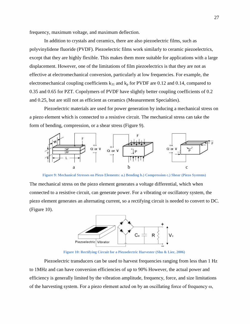
Piezoelectric materials are used for power generation by inducing a mechanical stress on
a piezo element which is connected to a resistive circuit. The mechanical stress can take the
form of bending, compression, or a shear stress (Figure 9).
Figure 9: Mechanical Stresses on Piezo Elements: a.) Bending b.) Compression c.) Shear (Piezo Systems)
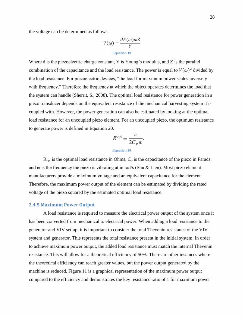
The mechanical stress on the piezo element generates a voltage differential, which when
connected to a resistive circuit, can generate power. For a vibrating or oscillatory system, the
piezo element generates an alternating current, so a rectifying circuit is needed to convert to DC.
(Figure 10).
Figure 10: Rectifying Circuit for a Piezoelectric Harvester (Shu & Lier, 2006)
Piezoelectric transducers can be used to harvest frequencies ranging from less than 1 Hz
to 1MHz and can have conversion efficiencies of up to 90% However, the actual power and
efficiency is generally limited by the vibration amplitude, frequency, force, and size limitations
of the harvesting system. For a piezo element acted on by an oscillating force of frequency ω,
a b c
28
the voltage can be determined as follows:
𝑉(𝜔) =𝑑𝐹(𝜔)𝜔𝑍
𝑌
Equation 19
Where d is the piezoelectric charge constant, Y is Young’s modulus, and Z is the parallel
combination of the capacitance and the load resistance. The power is equal to 𝑉(𝜔)2divided by
the load resistance. For piezoelectric devices, “the load for maximum power scales inversely
with frequency.” Therefore the frequency at which the object operates determines the load that
the system can handle (Sherrit, S., 2008). The optimal load resistance for power generation in a
piezo transducer depends on the equivalent resistance of the mechanical harvesting system it is
coupled with. However, the power generation can also be estimated by looking at the optimal
load resistance for an uncoupled piezo element. For an uncoupled piezo, the optimum resistance
to generate power is defined in Equation 20.
Equation 20
Ropt is the optimal load resistance in Ohms, Cp is the capacitance of the piezo in Farads,
and ω is the frequency the piezo is vibrating at in rad/s (Shu & Lien). Most piezo element
manufacturers provide a maximum voltage and an equivalent capacitance for the element.
Therefore, the maximum power output of the element can be estimated by dividing the rated
voltage of the piezo squared by the estimated optimal load resistance.
2.4.5 Maximum Power Output
A load resistance is required to measure the electrical power output of the system once it
has been converted from mechanical to electrical power. When adding a load resistance to the
generator and VIV set up, it is important to consider the total Thevenin resistance of the VIV
system and generator. This represents the total resistance present in the initial system. In order
to achieve maximum power output, the added load resistance must match the internal Thevenin
resistance. This will allow for a theoretical efficiency of 50%. There are other instances where
the theoretical efficiency can reach greater values, but the power output generated by the
machine is reduced. Figure 11 is a graphical representation of the maximum power output
compared to the efficiency and demonstrates the key resistance ratio of 1 for maximum power
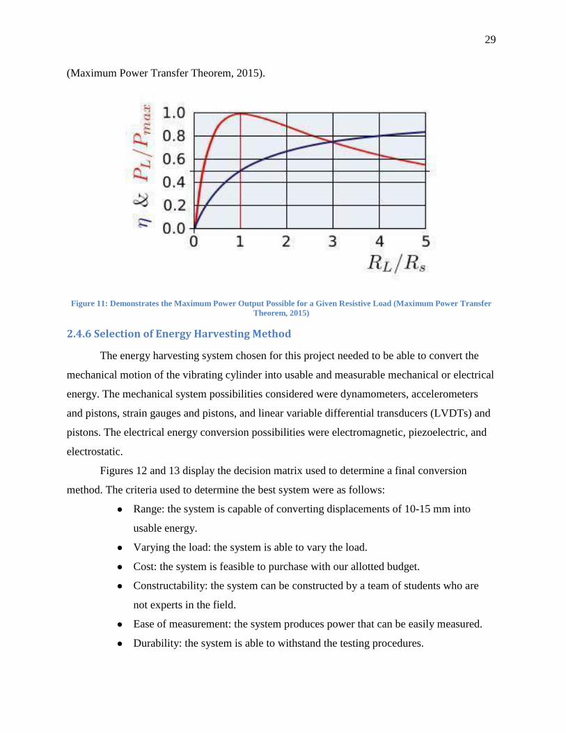
29
(Maximum Power Transfer Theorem, 2015).
Figure 11: Demonstrates the Maximum Power Output Possible for a Given Resistive Load (Maximum Power Transfer
Theorem, 2015)
2.4.6 Selection of Energy Harvesting Method
The energy harvesting system chosen for this project needed to be able to convert the
mechanical motion of the vibrating cylinder into usable and measurable mechanical or electrical
energy. The mechanical system possibilities considered were dynamometers, accelerometers
and pistons, strain gauges and pistons, and linear variable differential transducers (LVDTs) and
pistons. The electrical energy conversion possibilities were electromagnetic, piezoelectric, and
electrostatic.
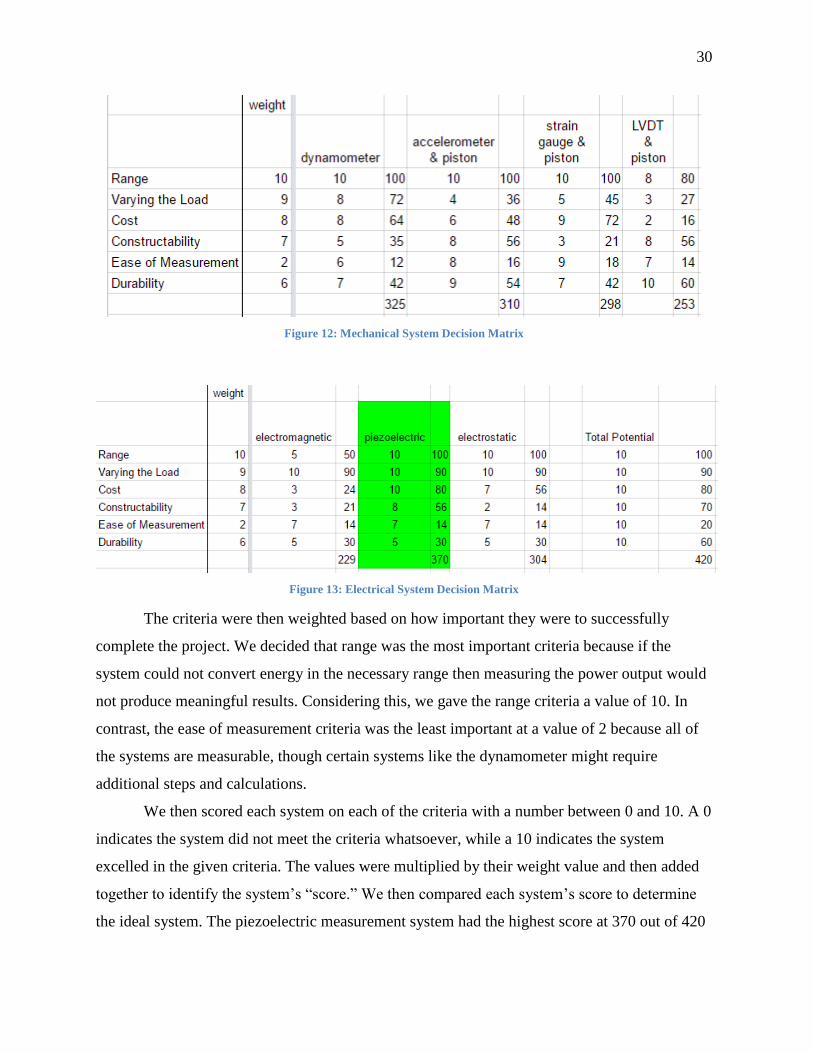
Figures 12 and 13 display the decision matrix used to determine a final conversion
method. The criteria used to determine the best system were as follows:
Range: the system is capable of converting displacements of 10-15 mm into
usable energy.
Varying the load: the system is able to vary the load.
Cost: the system is feasible to purchase with our allotted budget.
Constructability: the system can be constructed by a team of students who are
not experts in the field.
Ease of measurement: the system produces power that can be easily measured.
Durability: the system is able to withstand the testing procedures.
30
Figure 12: Mechanical System Decision Matrix
Figure 13: Electrical System Decision Matrix
The criteria were then weighted based on how important they were to successfully
complete the project. We decided that range was the most important criteria because if the
system could not convert energy in the necessary range then measuring the power output would
not produce meaningful results. Considering this, we gave the range criteria a value of 10. In
contrast, the ease of measurement criteria was the least important at a value of 2 because all of
the systems are measurable, though certain systems like the dynamometer might require
additional steps and calculations.
We then scored each system on each of the criteria with a number between 0 and 10. A 0
indicates the system did not meet the criteria whatsoever, while a 10 indicates the system
excelled in the given criteria. The values were multiplied by their weight value and then added
together to identify the system’s “score.” We then compared each system’s score to determine
the ideal system. The piezoelectric measurement system had the highest score at 370 out of 420

31
possible points. The electromagnetic system had the lowest score at 229 points out of the
possible 420.
The piezoelectric measurement system was scored the highest because it performed well
in the majority of the criteria. It was ranked high for range because there are multiple varieties
of piezoelectric materials, which would ensure data measurements in the needed range. It, along
with all of the electrical options, scored high for varying the load because this can be done by
simply changing the value of a resistor in the circuit. Lastly, piezoelectric material was given 7
out of 10 for ease of measurement because voltage can be easily measured with a multimeter,
but the electrical elements need to be waterproof.

32
3. Piezoelectric Testing and Prototyping
In order to produce power through oscillations, both the VIV oscillator and
piezoelectrics need to work independently. The first part of this chapter discusses choosing a
piezoelectric material and building a circuit to measure the voltage output of the piezoelectrics.
The second part of this chapter reviews the prototype building process and testing of the VIV
oscillator.
3.1 Piezoelectric Transducer Testing
There are numerous varieties of piezoelectric materials, ranging in cost and degree of
flexibility and sturdiness. In order to test the various kinds of piezoelectric materials and
determine the optimal positioning for the material of the system, we tested both ceramic and
film piezoelectric materials. The testing procedure for the piezoelectric transducers was an
iterative process that evolved as we learned more information. The piezoelectric films were
stressed by being pulled taut and inducing oscillating pulses, while the ceramic piezoelectric
disks were excited through bending the disks. The baseline testing involved the following
procedure:
1. Measure the voltage of each piezoelectric transducer directly with the oscilloscope to see
the unrectified voltage peaks.
2. Use the simulation program Multisim to model the rectifier circuit and note the expected
output. Include an internal capacitance value for the piezo equal to the value given in the
manufacturing specifications to properly model the system.
3. Set the Multisim inputs to 18 Vpk with a frequency of 6 Hz.
4. Use a function generator to ensure that the rectifier circuitry was functioning properly.
5. Set the function generator to 1 Vpk with a frequency of 2 Hz.
6. Plug piezoelectrics into the full bridge rectifying circuit, comprised of four 1N4148
diodes, a resistor that may be varied and a capacitor that may be varied.
7. Compare the results from the Multisim simulation and the actual rectifier circuit output.
8. Test each piezoelectric at resistance values from 5 MΩ to 15 MΩ and capacitor values
from 0.1 μF to 10 μF in order to assess the effect on the voltage output.
33
3.1.1 Measurement Methods
When attempting to measure the voltage peaks present in the circuit, we found that our
oscilloscope graphs were incorrect and would clip and offset the waveform. This was due to an
unavoidable grounding issue present in the circuit. The rectifier circuit is connected in a way
where the negative lead of the input is not connected to ground. The internal grounding of the
oscilloscope made it impossible to simultaneously measure both the input and the output
waveforms without seeing distortion because the circuit was already grounded. Therefore we
elected to measure the input with the oscilloscope and the output with the DMM (Digital
Multimeter). A second trial run was done for each test in order to also measure the output
waveform with the oscilloscope.
3.1.2 Full Bridge Rectifier
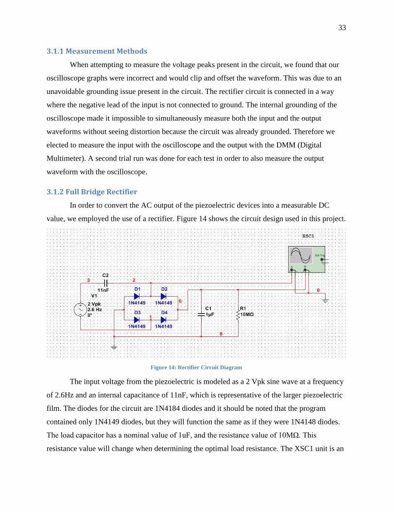
In order to convert the AC output of the piezoelectric devices into a measurable DC
value, we employed the use of a rectifier. Figure 14 shows the circuit design used in this project.
Figure 14: Rectifier Circuit Diagram
The input voltage from the piezoelectric is modeled as a 2 Vpk sine wave at a frequency
of 2.6Hz and an internal capacitance of 11nF, which is representative of the larger piezoelectric
film. The diodes for the circuit are 1N4184 diodes and it should be noted that the program
contained only 1N4149 diodes, but they will function the same as if they were 1N4148 diodes.
The load capacitor has a nominal value of 1uF, and the resistance value of 10MΩ. This
resistance value will change when determining the optimal load resistance. The XSC1 unit is an
34
oscilloscope, which is used to display the input and output waveforms. In order to ensure the
validity of this circuit design, we simulated it using Multisim, and produced the waveforms
shown in Figure 15.
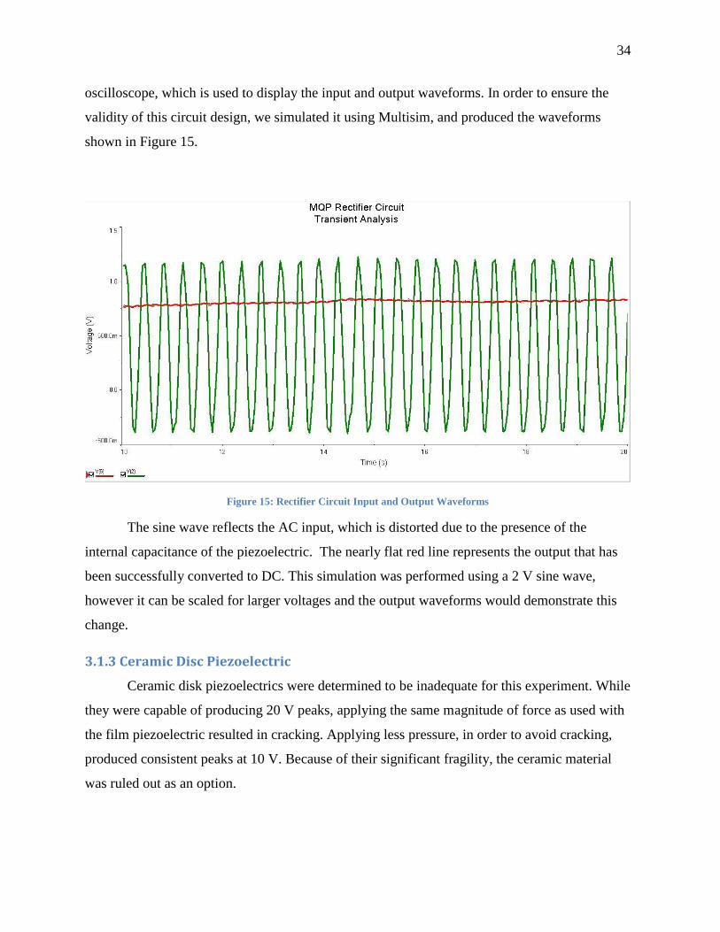
Figure 15: Rectifier Circuit Input and Output Waveforms
The sine wave reflects the AC input, which is distorted due to the presence of the
internal capacitance of the piezoelectric. The nearly flat red line represents the output that has
been successfully converted to DC. This simulation was performed using a 2 V sine wave,
however it can be scaled for larger voltages and the output waveforms would demonstrate this
change.
3.1.3 Ceramic Disc Piezoelectric
Ceramic disk piezoelectrics were determined to be inadequate for this experiment. While
they were capable of producing 20 V peaks, applying the same magnitude of force as used with
the film piezoelectric resulted in cracking. Applying less pressure, in order to avoid cracking,
produced consistent peaks at 10 V. Because of their significant fragility, the ceramic material
was ruled out as an option.
35
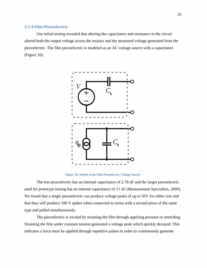
3.1.4 Film Piezoelectric
Our initial testing revealed that altering the capacitance and resistance in the circuit
altered both the output voltage across the resistor and the measured voltage generated from the
piezoelectric. The film piezoelectric is modeled as an AC voltage source with a capacitance
(Figure 16).
Figure 16: Model of the Film Piezoelectric Voltage Source
The test piezoelectric has an internal capacitance of 2.78 nF and the larger piezoelectric
used for prototype testing has an internal capacitance of 11 nF (Measurement Specialties, 2009).
We found that a single piezoelectric can produce voltage peaks of up to 50V for either size and
that they will produce 100 V spikes when connected in series with a second piezo of the same
type and pulled simultaneously.
The piezoelectric is excited by straining the film through applying pressure or stretching.
Straining the film under constant tension generated a voltage peak which quickly decayed. This
indicates a force must be applied through repetitive pulses in order to continuously generate
36
electricity. Due to the oscillatory nature of our project, this allowed the piezoelectric to generate
continuous electricity as the cylinder vibrated.
3.1.5 Power Output
We measured the voltage output of the piezoelectric used in the prototype when it was
not attached to a circuit. The piezoelectric was able to produce voltage peaks of approximately
50 V when sufficiently and consistently pulled taut. Pulling the piezoelectric at a force similar
to that expected in the prototype resulted in a voltage that was approximately 10 V. However,
this peak voltage is higher than the voltage output when the piezoelectric is connected to the
rectifier circuit. The power output can be calculated by dividing the square of the voltage by the
measured value of the resistance.
3.1.6 Circuit Components
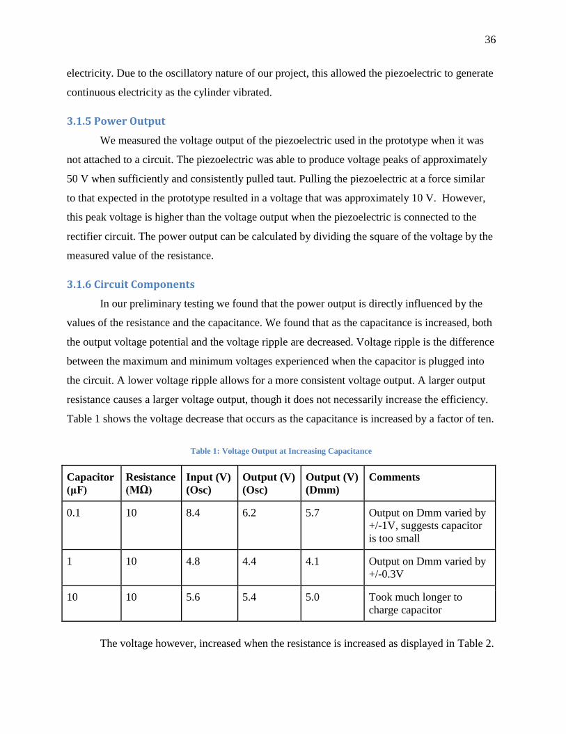
In our preliminary testing we found that the power output is directly influenced by the
values of the resistance and the capacitance. We found that as the capacitance is increased, both
the output voltage potential and the voltage ripple are decreased. Voltage ripple is the difference
between the maximum and minimum voltages experienced when the capacitor is plugged into
the circuit. A lower voltage ripple allows for a more consistent voltage output. A larger output
resistance causes a larger voltage output, though it does not necessarily increase the efficiency.
Table 1 shows the voltage decrease that occurs as the capacitance is increased by a factor of ten.
Table 1: Voltage Output at Increasing Capacitance
Capacitor
(μF)
Resistance
(MΩ)
Input (V)
(Osc)
Output (V)
(Osc)
Output (V)
(Dmm)
Comments
0.1 10 8.4 6.2 5.7 Output on Dmm varied by
+/-1V, suggests capacitor
is too small
1 10 4.8 4.4 4.1 Output on Dmm varied by
+/-0.3V
10 10 5.6 5.4 5.0 Took much longer to
charge capacitor
The voltage however, increased when the resistance is increased as displayed in Table 2.
37
Table 2: Voltage Output at Increasing Resistance
Resistance (MΩ) Capacitance (μF) Output Voltage (V) Power Output (μW)
5 1 2 0.8
10 1 3-5 0.9-3.0
15 1 3-5 0.6-2.0
From these resistance and voltage values, we calculated that the overall expected power output
is a range between 0.6 and 3 microwatts.
3.2 Oscillator Constraints and Design
The first part of this section outlines the various constraints and dimensions of the
testing location. The next part describes the design of the oscillator used as a base for all
prototypes.
3.2.1 Testing Location
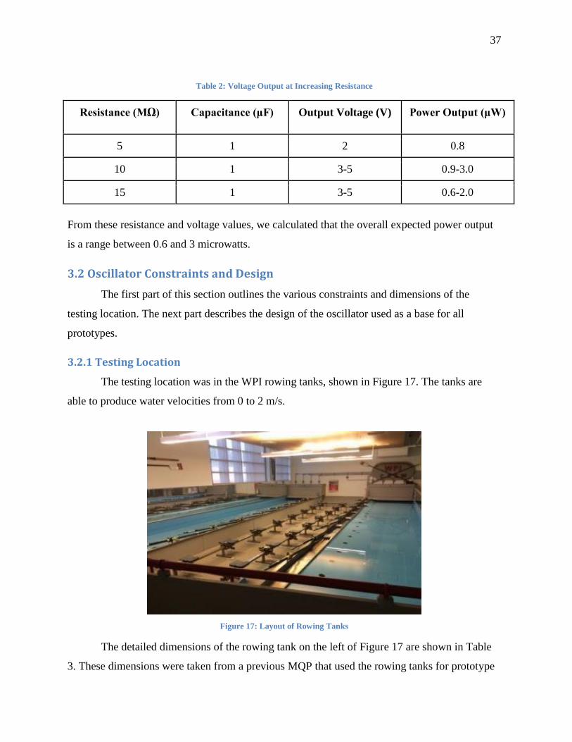
The testing location was in the WPI rowing tanks, shown in Figure 17. The tanks are
able to produce water velocities from 0 to 2 m/s.
Figure 17: Layout of Rowing Tanks
The detailed dimensions of the rowing tank on the left of Figure 17 are shown in Table
3. These dimensions were taken from a previous MQP that used the rowing tanks for prototype
38
testing (Costanzo, 2015).
Table 3: Rowing Tank Dimensions
Total Length (L) 47’ (14.3m)
Water depth at L = 0m 14.75” (0.37m)
Water depth at L = 7.62m 13.00” ( 0.33m)
Water depth at L = 14.33m 11.00” (0.28m)
Width of flat bottom 44” (1.12m)
Width of tank (including ledge) 100” (2.54m)
Height of narrow ledge from bottom at 0m 25” (0.635m)
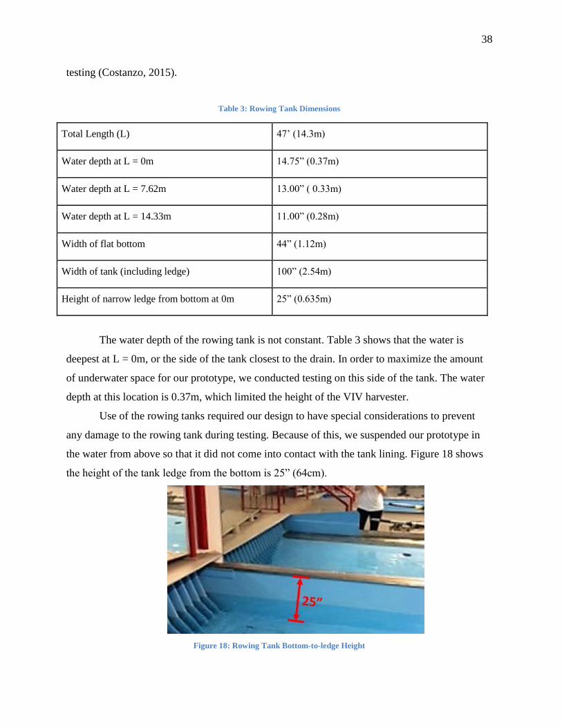
The water depth of the rowing tank is not constant. Table 3 shows that the water is
deepest at L = 0m, or the side of the tank closest to the drain. In order to maximize the amount
of underwater space for our prototype, we conducted testing on this side of the tank. The water
depth at this location is 0.37m, which limited the height of the VIV harvester.
Use of the rowing tanks required our design to have special considerations to prevent
any damage to the rowing tank during testing. Because of this, we suspended our prototype in
the water from above so that it did not come into contact with the tank lining. Figure 18 shows
the height of the tank ledge from the bottom is 25” (64cm).
Figure 18: Rowing Tank Bottom-to-ledge Height
39
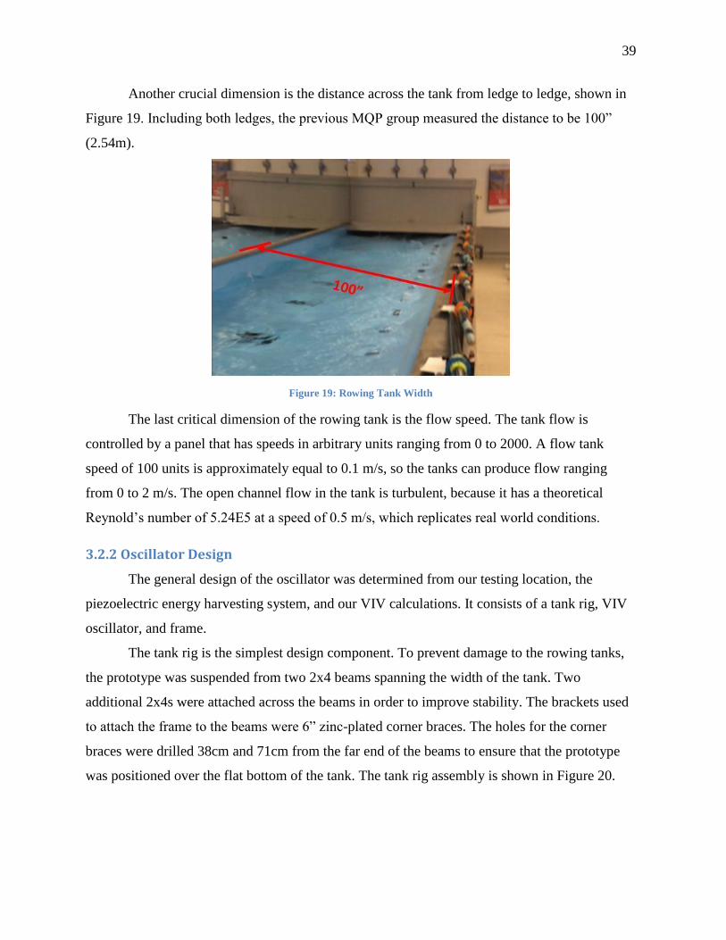
Another crucial dimension is the distance across the tank from ledge to ledge, shown in
Figure 19. Including both ledges, the previous MQP group measured the distance to be 100”
(2.54m).
Figure 19: Rowing Tank Width
The last critical dimension of the rowing tank is the flow speed. The tank flow is
controlled by a panel that has speeds in arbitrary units ranging from 0 to 2000. A flow tank
speed of 100 units is approximately equal to 0.1 m/s, so the tanks can produce flow ranging
from 0 to 2 m/s. The open channel flow in the tank is turbulent, because it has a theoretical
Reynold’s number of 5.24E5 at a speed of 0.5 m/s, which replicates real world conditions.
3.2.2 Oscillator Design
The general design of the oscillator was determined from our testing location, the
piezoelectric energy harvesting system, and our VIV calculations. It consists of a tank rig, VIV
oscillator, and frame.
The tank rig is the simplest design component. To prevent damage to the rowing tanks,
the prototype was suspended from two 2x4 beams spanning the width of the tank. Two
additional 2x4s were attached across the beams in order to improve stability. The brackets used
to attach the frame to the beams were 6” zinc-plated corner braces. The holes for the corner
braces were drilled 38cm and 71cm from the far end of the beams to ensure that the prototype
was positioned over the flat bottom of the tank. The tank rig assembly is shown in Figure 20.
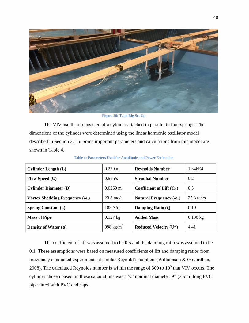
40
Figure 20: Tank Rig Set Up
The VIV oscillator consisted of a cylinder attached in parallel to four springs. The
dimensions of the cylinder were determined using the linear harmonic oscillator model
described in Section 2.1.5. Some important parameters and calculations from this model are
shown in Table 4.
Table 4: Parameters Used for Amplitude and Power Estimation
Cylinder Length (L) 0.229 m Reynolds Number 1.346E4
Flow Speed (U) 0.5 m/s Strouhal Number 0.2
Cylinder Diameter (D) 0.0269 m Coefficient of Lift (CL) 0.5
Vortex Shedding Frequency (ωs) 23.3 rad/s Natural Frequency (ωn) 25.3 rad/s
Spring Constant (k) 182 N/m Damping Ratio (ζ) 0.10
Mass of Pipe 0.127 kg Added Mass 0.130 kg
Density of Water (ρ) 998 kg/m3
Reduced Velocity (U*) 4.41
The coefficient of lift was assumed to be 0.5 and the damping ratio was assumed to be
0.1. These assumptions were based on measured coefficients of lift and damping ratios from
previously conducted experiments at similar Reynold’s numbers (Williamson & Govordhan,
2008). The calculated Reynolds number is within the range of 300 to 105 that VIV occurs. The
cylinder chosen based on these calculations was a ¾” nominal diameter, 9” (23cm) long PVC
pipe fitted with PVC end caps.
41
Given these values, the following equations were used to calculate the maximum
amplitude, lift force, and power output:
𝐴 =𝜌𝑈2𝐷𝐿𝐶𝐿
2𝑘 ∗ √[1− (ω𝑠/𝜔𝑛)2]2 + (2𝜁ω𝑠/𝜔𝑛)2)
𝐹𝐿 =1
2𝜌𝑈2𝐷𝐿𝐶𝐿
𝑃𝑚𝑎𝑥 =ω𝑠𝜌
2𝑈4𝐷2𝐿2𝐶𝐿2
4𝑘 ∗ √[1 − (ω𝑠/𝜔𝑛)2]2 + (2𝜁ω𝑠/𝜔𝑛)2)
Equation 21
From these equations, the maximum amplitude was calculated to be 7.4cm, the
maximum lift force was 0.38 N, and the maximum theoretical mechanical system power was
0.066 W.
The oscillator design used four springs connected in parallel to suspend the cylinder.
The desired spring constant for each spring was a quarter of the total spring constant of 182
N/m (Table 4). Therefore we chose each spring to have a value of 45.5 N/m. In order to handle
a maximum displacement of 7.4cm in either direction, the springs each needed to be able to
extend approximately 15cm from the starting position. Extension springs were found from
McMaster Carr with a stiffness of 42 N/m, an extended length of 18.6cm.
The final component of the design was the frame, which houses the oscillator and
connects to the tank rig. A model of the entire frame and tank rig assembly is shown in Figure
21.
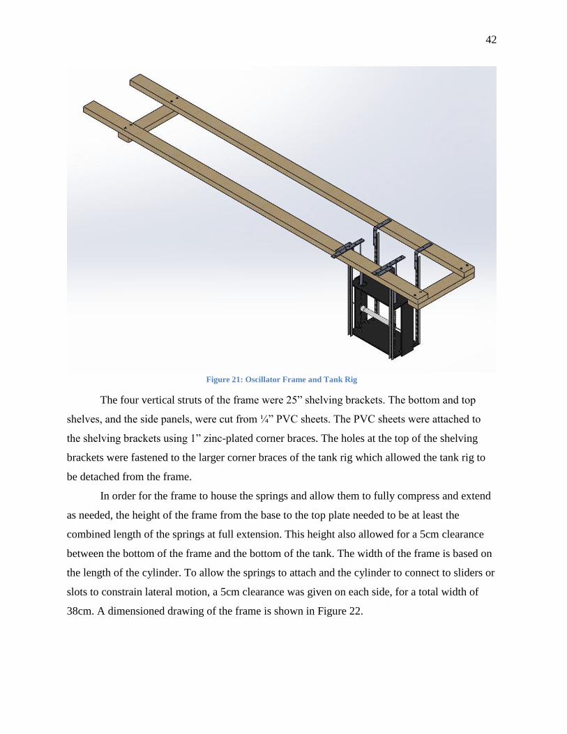
42
Figure 21: Oscillator Frame and Tank Rig
The four vertical struts of the frame were 25” shelving brackets. The bottom and top
shelves, and the side panels, were cut from ¼” PVC sheets. The PVC sheets were attached to
the shelving brackets using 1” zinc-plated corner braces. The holes at the top of the shelving
brackets were fastened to the larger corner braces of the tank rig which allowed the tank rig to
be detached from the frame.
In order for the frame to house the springs and allow them to fully compress and extend
as needed, the height of the frame from the base to the top plate needed to be at least the
combined length of the springs at full extension. This height also allowed for a 5cm clearance
between the bottom of the frame and the bottom of the tank. The width of the frame is based on
the length of the cylinder. To allow the springs to attach and the cylinder to connect to sliders or
slots to constrain lateral motion, a 5cm clearance was given on each side, for a total width of
38cm. A dimensioned drawing of the frame is shown in Figure 22.
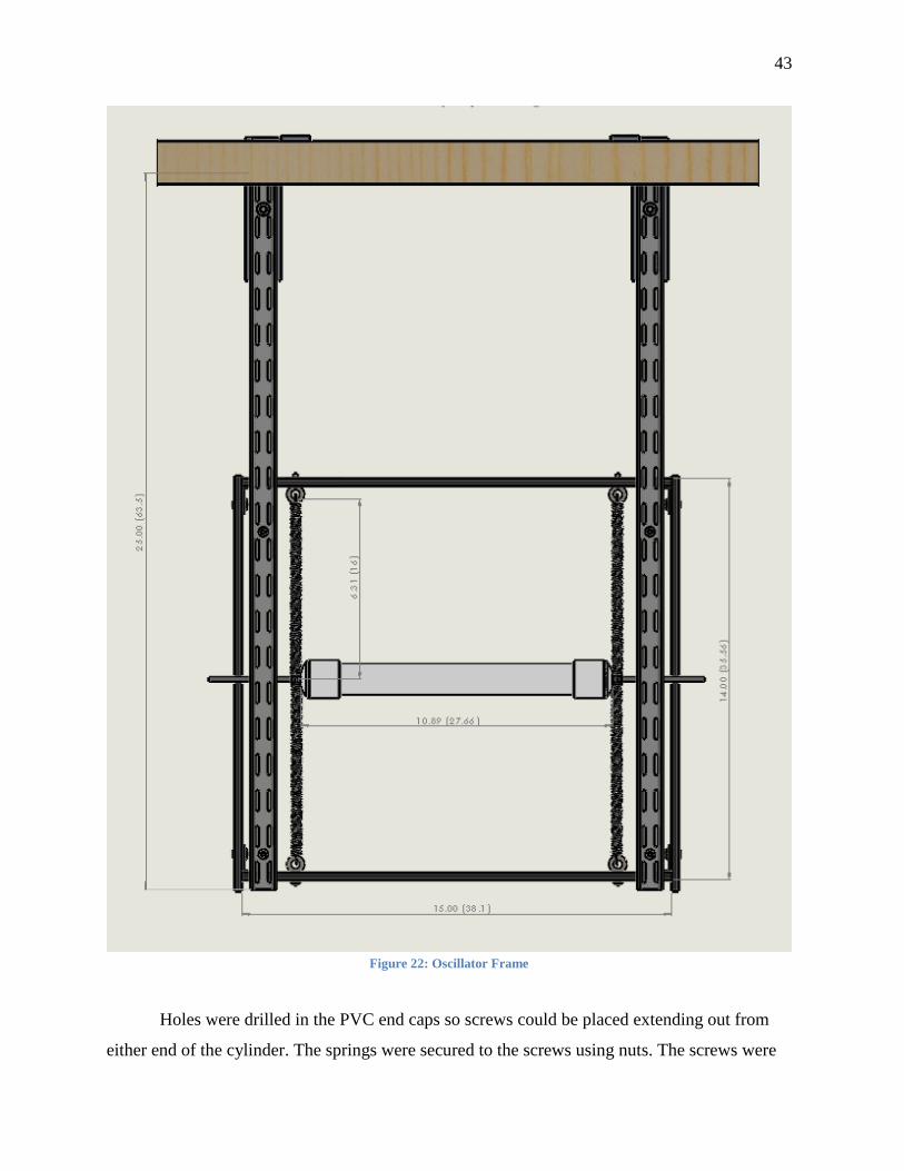
43
Figure 22: Oscillator Frame
Holes were drilled in the PVC end caps so screws could be placed extending out from
either end of the cylinder. The springs were secured to the screws using nuts. The screws were
44
also used to connect to various sliding and slot mechanisms used to constrain the cylinder
motion. These mechanisms are discussed in Section 3.4.
In order to measure the displacement of the cylinder visually, we attached a ruler to the
far side of the frame. A red wire that extended above the water level was attached to one of the
cylinder screws. When viewed from the side of the rowing tank, the wire was seen moving in
relation to the ruler and the displacement was measured.
3.3 Testing Procedures for Oscillator Prototypes
3.3.1 Flowing Water Tests
Each prototype was tested in flowing water in the rowing tanks to see if VIV occurred.
If oscillation was observed, the amplitude and frequency of the oscillations were measured
using a ruler, high speed camera, and Logger Pro’s video analysis tool. Each prototype was
tested using the following procedure:
1. Attach the ruler to the side of the oscillator.
2. Attach the pole with the netting to the end of the tank and lower the net so that it covers
the entrance to the drain.
3. Attach the oscillator to the wood frame and suspend the assembly in the water.
4. Set up the high speed camera on a tripod and position it so that the red wire attached to
the cylinder and the ruler are clearly visible and in focus.
5. Turn the rowing tanks to the lowest speed setting, which is about 100. Wait until the
water is flowing in the correct direction. This can take several minutes as the rowing
tank builds up speed.
6. Increase the speed of the flow by increments of 50. At each interval wait at least two
minutes for the flow to reach a constant speed.
7. If oscillation is observed record a video, clearly stating what speed the tank is set at.
Record at least 3 videos at each speed. Once any oscillation has been observed, record
videos of every subsequent speed.
8. Continue this process up to a tank setting of 800 or until the cylinder ceases to vibrate.
9. Once all the videos have been taken, turn the speed of the rowing tanks down to zero
and ensure that the screen has gone blank and the tanks are turned off.
45
10. Remove the entire apparatus from the water and detach the oscillator prototype from the
wood frame.
11. Import each video into Logger Pro and use the video analysis tool to plot the motion of
the red wire in the vertical direction. Use the ruler to set the scale on the video and the
tip of the red wire as the reference point.
12. Perform a sine function curve fit on the graph to obtain the frequency and average
amplitude of the oscillations.
13. Record the maximum and minimum displacement.
3.3.2 Still Water Tests
The damping coefficient and damped natural frequency of each oscillator prototype was
tested by measuring the oscillations of the cylinder in still water using the following procedure:
1. Attach the ruler to the side of the oscillator.
2. Submerge the oscillator in water.
3. Set up the high speed camera on a tripod and position it so that the red wire attached to
the cylinder and the ruler are clearly visible and in focus.
4. Start recording a video on the camera. Push the cylinder down approximately two inches
and release.
5. Wait for the oscillations to stop, and then push the cylinder up approximately two inches
and release.
6. Repeat steps 5 and 6 at least 5 times.
7. Stop recording, remove the entire apparatus from the water, and detach the oscillator
prototype from the wood frame.
8. Import the video into Logger Pro and use the video analysis tool to plot the motion of
the red wire in the vertical direction. Use the ruler to set the scale on the video and the
tip of the red wire as the reference point.
9. Perform a damped harmonic oscillator curve fit on the y-direction displacement graph to
obtain the damped natural frequency.
10. Measure the amplitude of two successive peaks on the graph and use the logarithmic
decrement method from Equation 6 to calculate the damping coefficient of the system. If
possible, repeat this process for each set of peaks of the oscillation before it converges to
zero.

46
11. Calculate the undamped natural frequency of the system using the measured damped
natural frequency and the damping coefficient.
12. Calculate both the total mass of the system using the natural frequency and total spring
stiffness and the mass ratio using Equations 3 and 4.
3.4 Oscillator Prototypes
The original frame and testing rig design, including the cylinder dimensions, remained
unchanged during prototype testing. However, the method of constraining the cylinder
movement was varied in order to achieve oscillation. These changes are detailed in the
following sections.
3.4.1 Prototype #1: Drawer Sliders Design
3.4.1.1 Design
The sliders used in this prototype are 22” Liberty Full Extension Ball Bearing Side
Mount Drawer Slides, shown in Figure 23. Holes in the base of the sliders were utilized to
attach to the PVC side panels. Slots were cut in the top PVC shelf to accommodate the top of
the sliders, which protrude above the shelf. The moving component of the slider was cut down
to its minimum possible length of 10” in order to reduce the mass of the cylinder assembly.
Holes in this moving slider were used to mount the screws that connect to the cylinder end caps.
Figure 23: Drawer Sliders
3.4.1.2 Results
The original drawer slider design was tested twice. In the first test, the flowing water
testing procedure outlined in Section 3.3.1 was conducted, but VIV did not occur in the system.
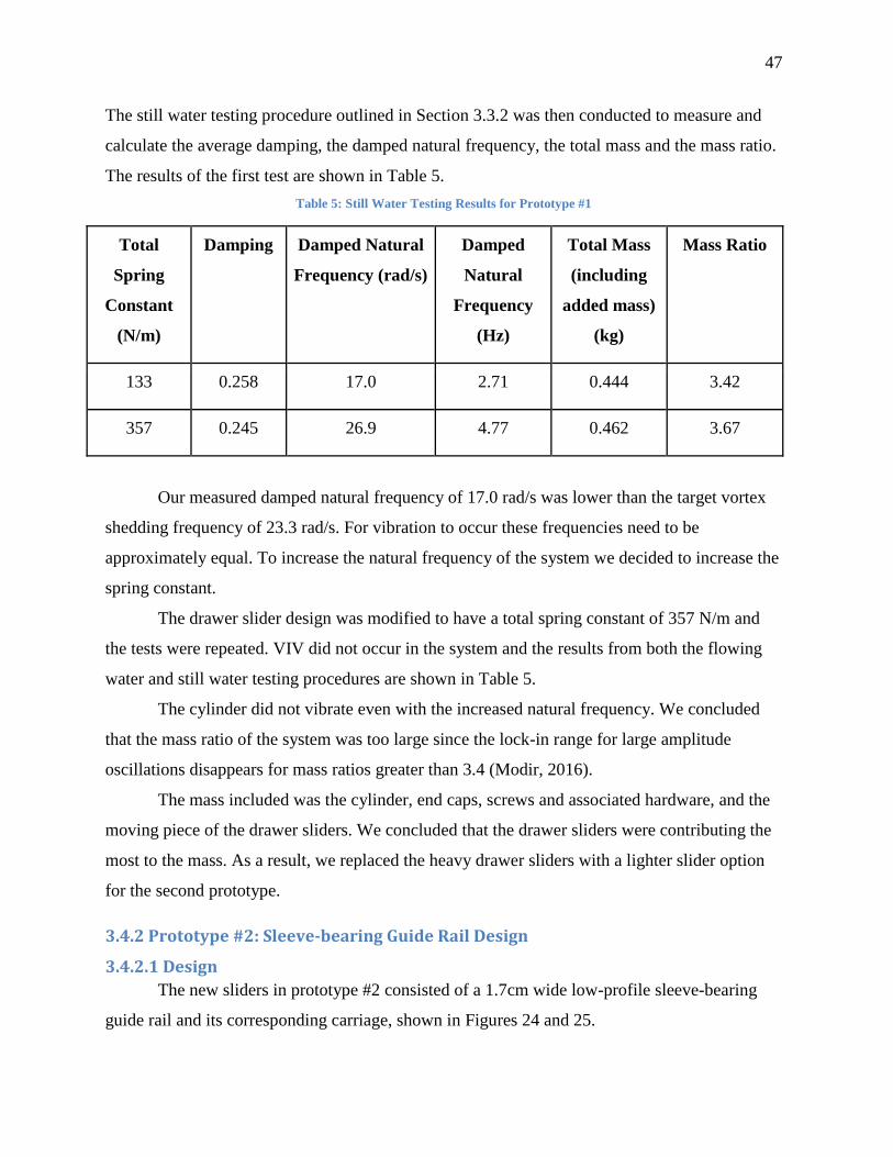
47
The still water testing procedure outlined in Section 3.3.2 was then conducted to measure and
calculate the average damping, the damped natural frequency, the total mass and the mass ratio.
The results of the first test are shown in Table 5.
Table 5: Still Water Testing Results for Prototype #1
Total
Spring
Constant
(N/m)
Damping Damped Natural
Frequency (rad/s)
Damped
Natural
Frequency
(Hz)
Total Mass
(including
added mass)
(kg)
Mass Ratio
133 0.258 17.0 2.71 0.444 3.42
357 0.245 26.9 4.77 0.462 3.67
Our measured damped natural frequency of 17.0 rad/s was lower than the target vortex
shedding frequency of 23.3 rad/s. For vibration to occur these frequencies need to be
approximately equal. To increase the natural frequency of the system we decided to increase the
spring constant.
The drawer slider design was modified to have a total spring constant of 357 N/m and
the tests were repeated. VIV did not occur in the system and the results from both the flowing
water and still water testing procedures are shown in Table 5.
The cylinder did not vibrate even with the increased natural frequency. We concluded
that the mass ratio of the system was too large since the lock-in range for large amplitude
oscillations disappears for mass ratios greater than 3.4 (Modir, 2016).
The mass included was the cylinder, end caps, screws and associated hardware, and the
moving piece of the drawer sliders. We concluded that the drawer sliders were contributing the
most to the mass. As a result, we replaced the heavy drawer sliders with a lighter slider option
for the second prototype.
3.4.2 Prototype #2: Sleeve-bearing Guide Rail Design
3.4.2.1 Design
The new sliders in prototype #2 consisted of a 1.7cm wide low-profile sleeve-bearing
guide rail and its corresponding carriage, shown in Figures 24 and 25.

48
Figure 24: Sleeve-bearing guide rail from McMaster-Carr
Figure 25: Sleeve-bearing carriage from McMaster-Carr
As in the previous prototype, the side panels were used to mount the guide rails. The
screws in the cylinder end caps were changed to M3 screws in order to fit the threaded holes in
the carriages. Instead of a single screw on each side of the cylinder as in prototype 1, two
screws were mounted in the cylinder end caps in order to balance the forces on the carriage
when the cylinder moves.
3.4.2.2 Results
Prototype #2 was not tested in the rowing tank because the sliders were unable to move
vertically without one side becoming stuck. The narrow tolerance of the carriage and rail caused
the carriage to stick when it did not move exactly parallel to the rail. Since the cylinder could
not remain perfectly horizontal when oscillating, the carriages could not be kept parallel and the
sliders were unusable.
3.4.3 Prototype #3: Freely Suspended Cylinder Design
3.4.3.1 Design
In the third prototype, sliders were abandoned altogether due to the frictional and mass
issues experienced in previous prototypes. The cylinder was allowed to move freely in any
direction, constrained only by the extension of the springs.
3.4.3.2 Results
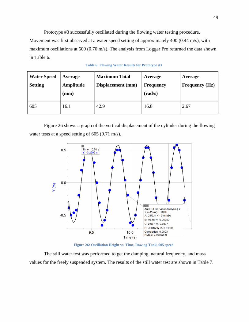
49
Prototype #3 successfully oscillated during the flowing water testing procedure.
Movement was first observed at a water speed setting of approximately 400 (0.44 m/s), with
maximum oscillations at 600 (0.70 m/s). The analysis from Logger Pro returned the data shown
in Table 6.
Table 6: Flowing Water Results for Prototype #3
Water Speed
Setting
Average
Amplitude
(mm)
Maximum Total
Displacement (mm)
Average
Frequency
(rad/s)
Average
Frequency (Hz)
605 16.1 42.9 16.8 2.67
Figure 26 shows a graph of the vertical displacement of the cylinder during the flowing
water tests at a speed setting of 605 (0.71 m/s).
Figure 26: Oscillation Height vs. Time, Rowing Tank, 605 speed
The still water test was performed to get the damping, natural frequency, and mass
values for the freely suspended system. The results of the still water test are shown in Table 7.
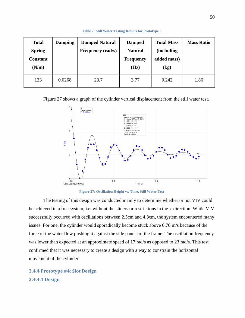
50
Table 7: Still Water Testing Results for Prototype 3
Total
Spring
Constant
(N/m)
Damping Damped Natural
Frequency (rad/s)
Damped
Natural
Frequency
(Hz)
Total Mass
(including
added mass)
(kg)
Mass Ratio
133 0.0268 23.7 3.77 0.242 1.86
Figure 27 shows a graph of the cylinder vertical displacement from the still water test.
Figure 27: Oscillation Height vs. Time, Still Water Test
The testing of this design was conducted mainly to determine whether or not VIV could
be achieved in a free system, i.e. without the sliders or restrictions in the x-direction. While VIV
successfully occurred with oscillations between 2.5cm and 4.3cm, the system encountered many
issues. For one, the cylinder would sporadically become stuck above 0.70 m/s because of the
force of the water flow pushing it against the side panels of the frame. The oscillation frequency
was lower than expected at an approximate speed of 17 rad/s as opposed to 23 rad/s. This test
confirmed that it was necessary to create a design with a way to constrain the horizontal
movement of the cylinder.
3.4.4 Prototype #4: Slot Design
3.4.4.1 Design
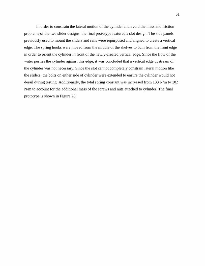
51
In order to constrain the lateral motion of the cylinder and avoid the mass and friction
problems of the two slider designs, the final prototype featured a slot design. The side panels
previously used to mount the sliders and rails were repurposed and aligned to create a vertical
edge. The spring hooks were moved from the middle of the shelves to 5cm from the front edge
in order to orient the cylinder in front of the newly-created vertical edge. Since the flow of the
water pushes the cylinder against this edge, it was concluded that a vertical edge upstream of
the cylinder was not necessary. Since the slot cannot completely constrain lateral motion like
the sliders, the bolts on either side of cylinder were extended to ensure the cylinder would not
derail during testing. Additionally, the total spring constant was increased from 133 N/m to 182
N/m to account for the additional mass of the screws and nuts attached to cylinder. The final
prototype is shown in Figure 28.
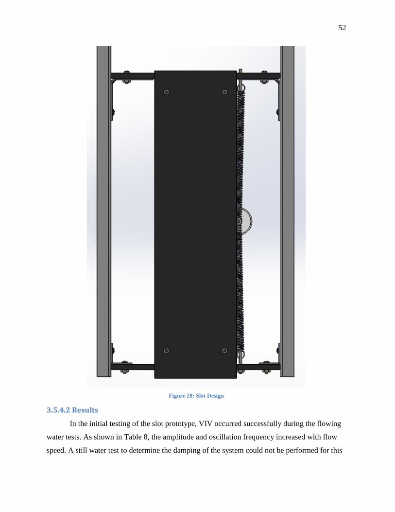
52
Figure 28: Slot Design
3.5.4.2 Results
In the initial testing of the slot prototype, VIV occurred successfully during the flowing
water tests. As shown in Table 8, the amplitude and oscillation frequency increased with flow
speed. A still water test to determine the damping of the system could not be performed for this
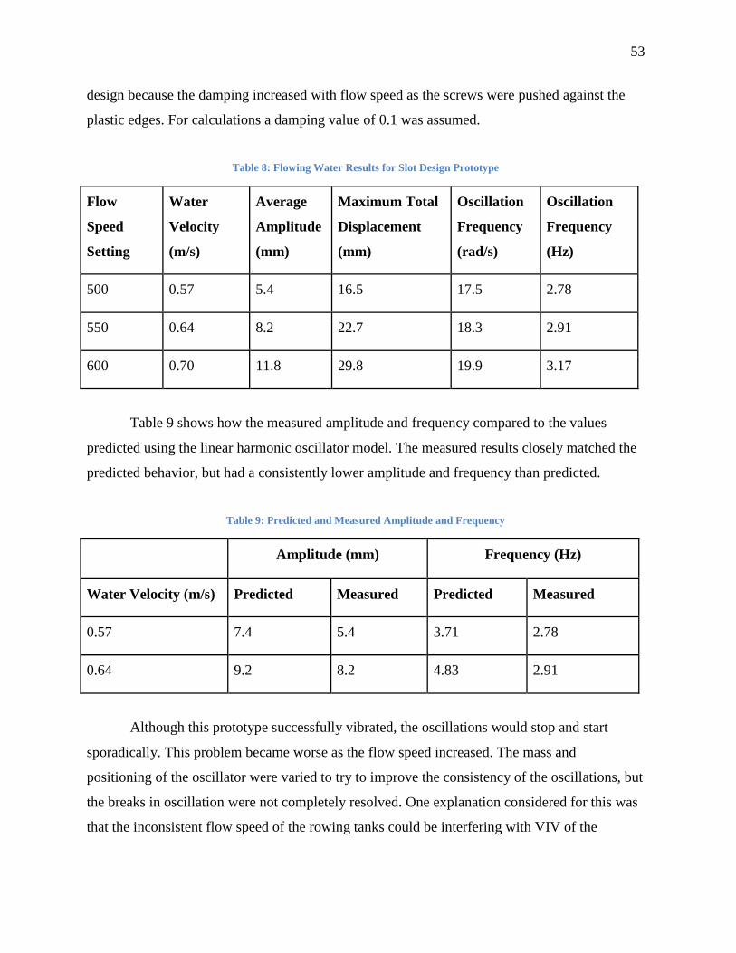
53
design because the damping increased with flow speed as the screws were pushed against the
plastic edges. For calculations a damping value of 0.1 was assumed.
Table 8: Flowing Water Results for Slot Design Prototype
Flow
Speed
Setting
Water
Velocity
(m/s)
Average
Amplitude
(mm)
Maximum Total
Displacement
(mm)
Oscillation
Frequency
(rad/s)
Oscillation
Frequency
(Hz)
500 0.57 5.4 16.5 17.5 2.78
550 0.64 8.2 22.7 18.3 2.91
600 0.70 11.8 29.8 19.9 3.17
Table 9 shows how the measured amplitude and frequency compared to the values
predicted using the linear harmonic oscillator model. The measured results closely matched the
predicted behavior, but had a consistently lower amplitude and frequency than predicted.
Table 9: Predicted and Measured Amplitude and Frequency
Amplitude (mm) Frequency (Hz)
Water Velocity (m/s) Predicted Measured Predicted Measured
0.57 7.4 5.4 3.71 2.78
0.64 9.2 8.2 4.83 2.91
Although this prototype successfully vibrated, the oscillations would stop and start
sporadically. This problem became worse as the flow speed increased. The mass and
positioning of the oscillator were varied to try to improve the consistency of the oscillations, but
the breaks in oscillation were not completely resolved. One explanation considered for this was
that the inconsistent flow speed of the rowing tanks could be interfering with VIV of the

54
cylinder. The team therefore decided to obtain a water velocity probe in order to be able to
measure the water velocity over time.
55
4. Methodology
The goal of this project was to utilize piezoelectric transducers to transform the VIV
oscillations of a cylinder to electrical power. We achieved this goal by following these
objectives:
1. Construct piezoelectric oscillator system using conclusions from preliminary testing.
2. Conduct flowing water testing to determine the water’s velocity.
3. Determine the optimal load resistance of the VIV system.
4.1 Energy Harvester Design The final energy harvester design consisted of two piezoelectric transducers attached to
the final oscillator prototype. Two 10” flat mending plates were attached to the wooden beams
of the frame so that they extended over oscillator. Five inch screws were connected to the
mending plates. Each piezoelectric transducer was epoxied to a 2” corner brace, which was
attached to the screws using two nuts. The top of each piezo was also coated in silicone gel to
waterproof the electrical leads.
Large holes were cut in the top plate of the oscillator so that the top set of springs could
extend through the plate unobstructed. The bottom of each piezoelectric was then epoxied to the
top of the springs. In this setup the piezoelectrics act as two additional springs in series with the
top set of springs and help to suspend the cylinder, as seen in Figure 29. The piezoelectrics each
had an effective spring constant of 66 MN/m. When connected in series with the top springs the
total spring constant for the system was 182 N/m, which was exactly the same as the total spring
constant for the oscillating system with no piezoelectrics attached. Several iterations of the
harvester design were tried with the piezoelectrics attached in parallel to the springs. The
cylinder did not vibrate with the parallel setup because the system spring constant was increased
to 131.8 MN/m. This spring constant would require a flow speed of 481 m/s, which is well
beyond any reasonable flow.

56
Figure 29: Connection of Piezoelectrics to the Oscillator
The piezoelectrics electrical leads were connected in series using alligator clips, and they
were attached to the rectifying circuit using two wires that ran the length of the wooden frame.
The rectifying circuit was kept in a waterproof container and attached to the wooden frame
outside of the tanks using velcro. Two wires extended outside of the container that were
connected to a multimeter in order to measure the output voltage.
4.2 Flowing Water Testing Procedure
The flow speed of the rowing tanks was measured using a Vernier velocity sensor. The
velocity sensor was attached using a pipe bracket and was positioned so that the sensor was
18cm from the bottom of the tank and 98cm from the mirrored wall. The velocity sensor was
used to measure the water velocity of the tanks at flow speeds of 200, 300, 400, 500, 550, 600,
and 650. The initial water level of the tanks was measured using a measuring tape. The tank
speed was then increased incrementally and the water velocity was recorded for two minutes at
each speed. Because the oscillator worked the best at a tank speed setting of 600, the team
recorded 10 minutes of velocity data at this setting. The testing setup is shown in Figure 30.
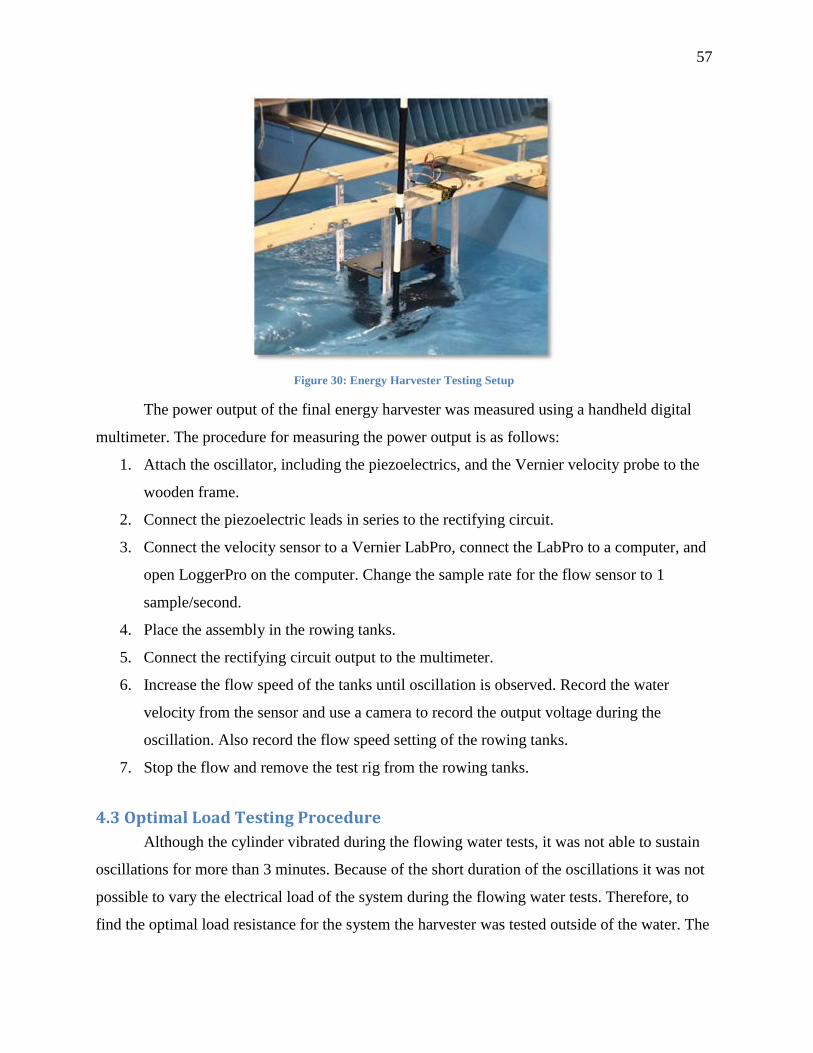
57
Figure 30: Energy Harvester Testing Setup
The power output of the final energy harvester was measured using a handheld digital
multimeter. The procedure for measuring the power output is as follows:
1. Attach the oscillator, including the piezoelectrics, and the Vernier velocity probe to the
wooden frame.
2. Connect the piezoelectric leads in series to the rectifying circuit.
3. Connect the velocity sensor to a Vernier LabPro, connect the LabPro to a computer, and
open LoggerPro on the computer. Change the sample rate for the flow sensor to 1
sample/second.
4. Place the assembly in the rowing tanks.
5. Connect the rectifying circuit output to the multimeter.
6. Increase the flow speed of the tanks until oscillation is observed. Record the water
velocity from the sensor and use a camera to record the output voltage during the
oscillation. Also record the flow speed setting of the rowing tanks.
7. Stop the flow and remove the test rig from the rowing tanks.
4.3 Optimal Load Testing Procedure
Although the cylinder vibrated during the flowing water tests, it was not able to sustain
oscillations for more than 3 minutes. Because of the short duration of the oscillations it was not
possible to vary the electrical load of the system during the flowing water tests. Therefore, to
find the optimal load resistance for the system the harvester was tested outside of the water. The
58
piezoelectrics were connected to the rectifying circuit and the cylinder was oscillated by hand to
a displacement of 0.5” (1.3cm) at an approximate frequency of 2.6 Hz. A ruler was used to
ensure the correct displacement and a metronome was used to move the cylinder at the desired
frequency. The output of the rectifying circuit was connected to an oscilloscope which was used
to measure the output voltage. The load resistance was varied from 511 kΩ to 32 MΩ and the
voltage was recorded. The power output for each resistance was calculated using 𝑃 =𝑉2
𝑅, where
V is the voltage and R is the resistance.
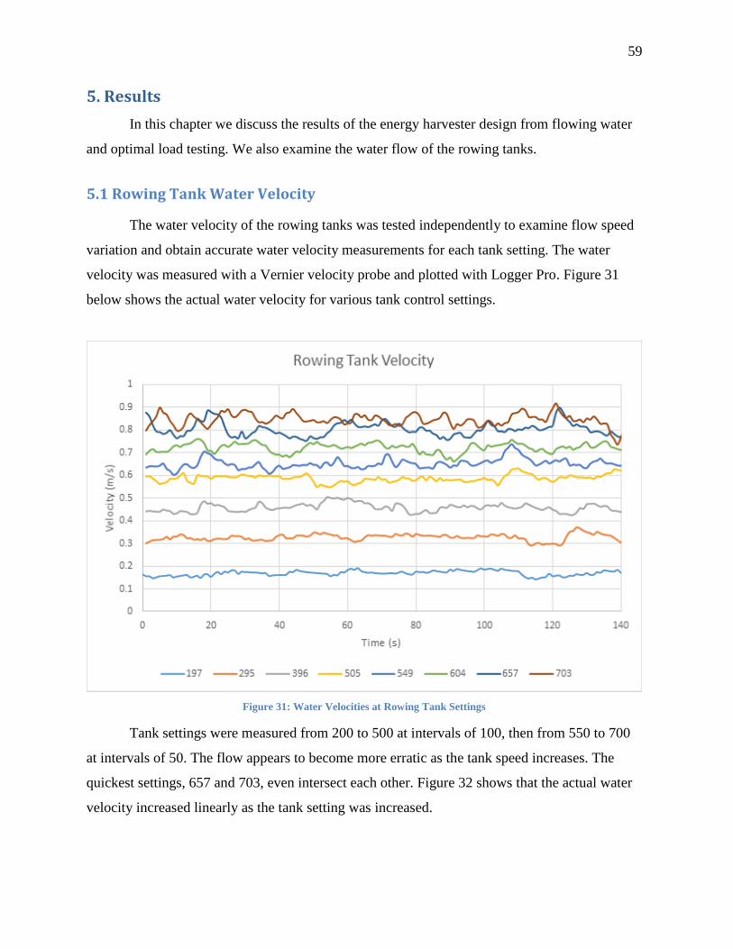
59
5. Results
In this chapter we discuss the results of the energy harvester design from flowing water
and optimal load testing. We also examine the water flow of the rowing tanks.
5.1 Rowing Tank Water Velocity
The water velocity of the rowing tanks was tested independently to examine flow speed
variation and obtain accurate water velocity measurements for each tank setting. The water
velocity was measured with a Vernier velocity probe and plotted with Logger Pro. Figure 31
below shows the actual water velocity for various tank control settings.
Figure 31: Water Velocities at Rowing Tank Settings
Tank settings were measured from 200 to 500 at intervals of 100, then from 550 to 700
at intervals of 50. The flow appears to become more erratic as the tank speed increases. The
quickest settings, 657 and 703, even intersect each other. Figure 32 shows that the actual water
velocity increased linearly as the tank setting was increased.
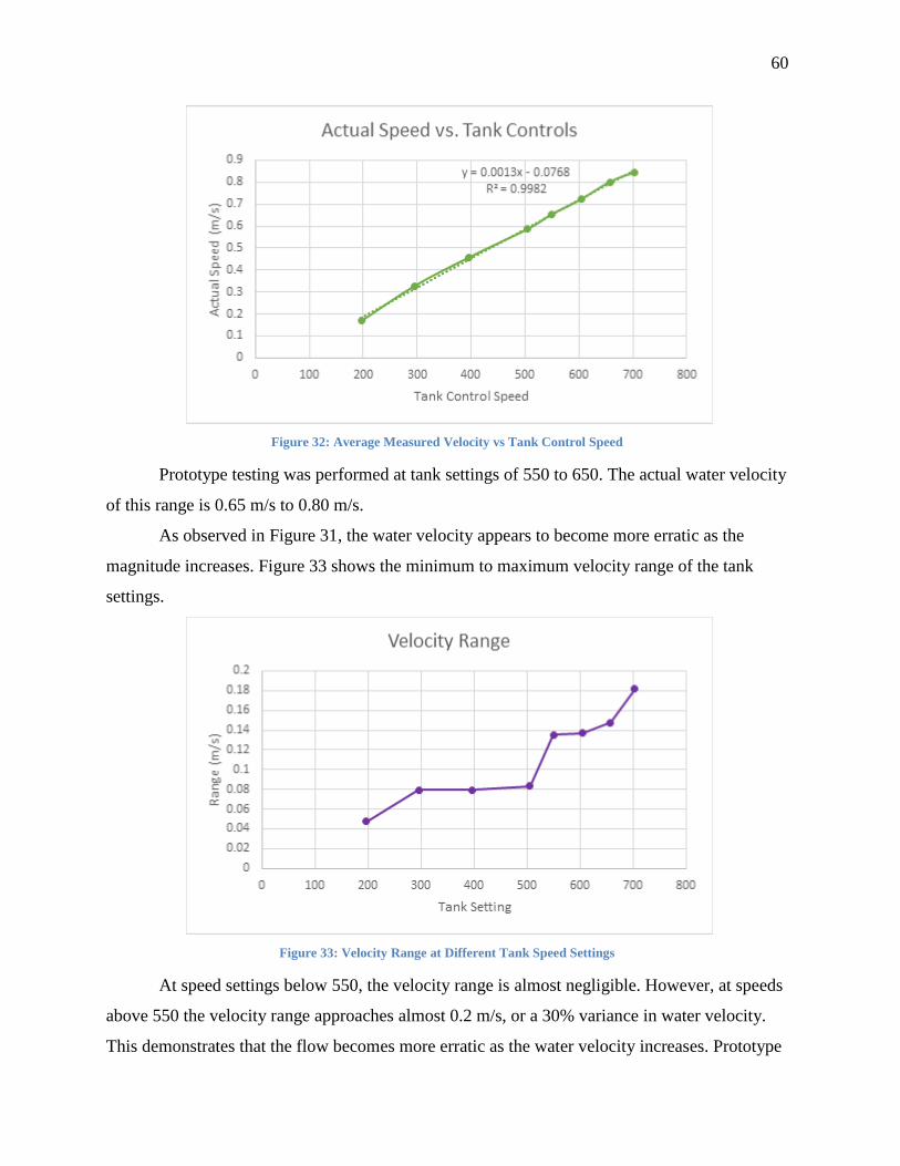
60
Figure 32: Average Measured Velocity vs Tank Control Speed
Prototype testing was performed at tank settings of 550 to 650. The actual water velocity
of this range is 0.65 m/s to 0.80 m/s.
As observed in Figure 31, the water velocity appears to become more erratic as the
magnitude increases. Figure 33 shows the minimum to maximum velocity range of the tank
settings.
Figure 33: Velocity Range at Different Tank Speed Settings
At speed settings below 550, the velocity range is almost negligible. However, at speeds
above 550 the velocity range approaches almost 0.2 m/s, or a 30% variance in water velocity.
This demonstrates that the flow becomes more erratic as the water velocity increases. Prototype
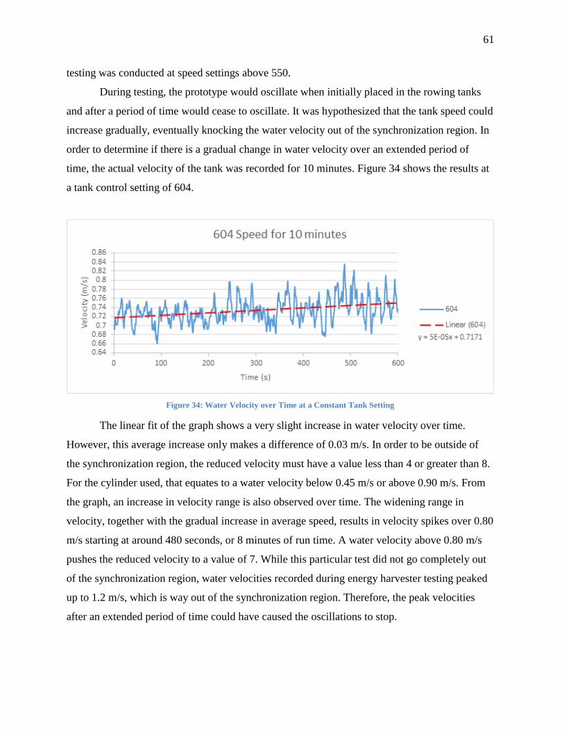
61
testing was conducted at speed settings above 550.
During testing, the prototype would oscillate when initially placed in the rowing tanks
and after a period of time would cease to oscillate. It was hypothesized that the tank speed could
increase gradually, eventually knocking the water velocity out of the synchronization region. In
order to determine if there is a gradual change in water velocity over an extended period of
time, the actual velocity of the tank was recorded for 10 minutes. Figure 34 shows the results at
a tank control setting of 604.
Figure 34: Water Velocity over Time at a Constant Tank Setting
The linear fit of the graph shows a very slight increase in water velocity over time.
However, this average increase only makes a difference of 0.03 m/s. In order to be outside of
the synchronization region, the reduced velocity must have a value less than 4 or greater than 8.
For the cylinder used, that equates to a water velocity below 0.45 m/s or above 0.90 m/s. From
the graph, an increase in velocity range is also observed over time. The widening range in
velocity, together with the gradual increase in average speed, results in velocity spikes over 0.80
m/s starting at around 480 seconds, or 8 minutes of run time. A water velocity above 0.80 m/s
pushes the reduced velocity to a value of 7. While this particular test did not go completely out
of the synchronization region, water velocities recorded during energy harvester testing peaked
up to 1.2 m/s, which is way out of the synchronization region. Therefore, the peak velocities
after an extended period of time could have caused the oscillations to stop.
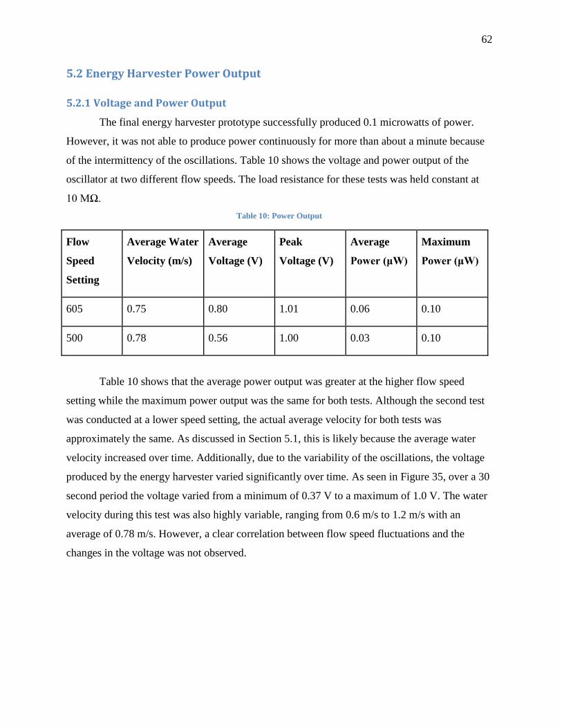
62
5.2 Energy Harvester Power Output
5.2.1 Voltage and Power Output
The final energy harvester prototype successfully produced 0.1 microwatts of power.
However, it was not able to produce power continuously for more than about a minute because
of the intermittency of the oscillations. Table 10 shows the voltage and power output of the
oscillator at two different flow speeds. The load resistance for these tests was held constant at
10 MΩ.
Table 10: Power Output
Flow
Speed
Setting
Average Water
Velocity (m/s)
Average
Voltage (V)
Peak
Voltage (V)
Average
Power (μW)
Maximum
Power (μW)
605 0.75 0.80 1.01 0.06 0.10
500 0.78 0.56 1.00 0.03 0.10
Table 10 shows that the average power output was greater at the higher flow speed
setting while the maximum power output was the same for both tests. Although the second test
was conducted at a lower speed setting, the actual average velocity for both tests was
approximately the same. As discussed in Section 5.1, this is likely because the average water
velocity increased over time. Additionally, due to the variability of the oscillations, the voltage
produced by the energy harvester varied significantly over time. As seen in Figure 35, over a 30
second period the voltage varied from a minimum of 0.37 V to a maximum of 1.0 V. The water
velocity during this test was also highly variable, ranging from 0.6 m/s to 1.2 m/s with an
average of 0.78 m/s. However, a clear correlation between flow speed fluctuations and the
changes in the voltage was not observed.
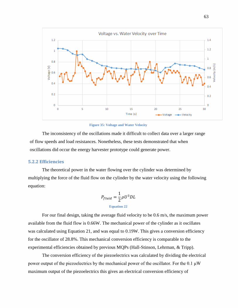
63
Figure 35: Voltage and Water Velocity
The inconsistency of the oscillations made it difficult to collect data over a larger range
of flow speeds and load resistances. Nonetheless, these tests demonstrated that when
oscillations did occur the energy harvester prototype could generate power.
5.2.2 Efficiencies
The theoretical power in the water flowing over the cylinder was determined by
multiplying the force of the fluid flow on the cylinder by the water velocity using the following
equation:
𝑃𝑓𝑙𝑢𝑖𝑑 =1
2𝜌𝑈3𝐷𝐿
Equation 22
For our final design, taking the average fluid velocity to be 0.6 m/s, the maximum power
available from the fluid flow is 0.66W. The mechanical power of the cylinder as it oscillates
was calculated using Equation 21, and was equal to 0.19W. This gives a conversion efficiency
for the oscillator of 28.8%. This mechanical conversion efficiency is comparable to the
experimental efficiencies obtained by previous MQPs (Hall-Stinson, Lehrman, & Tripp).
The conversion efficiency of the piezoelectrics was calculated by dividing the electrical
power output of the piezoelectrics by the mechanical power of the oscillator. For the 0.1 μW
maximum output of the piezoelectrics this gives an electrical conversion efficiency of
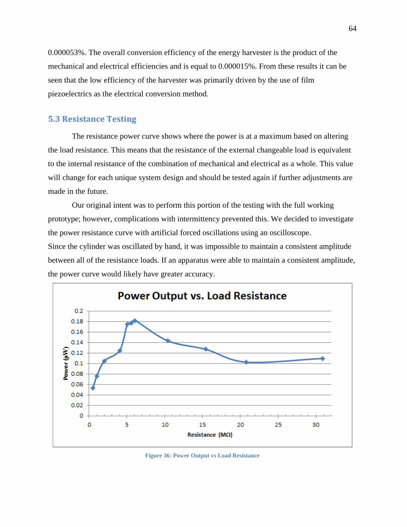
64
0.000053%. The overall conversion efficiency of the energy harvester is the product of the
mechanical and electrical efficiencies and is equal to 0.000015%. From these results it can be
seen that the low efficiency of the harvester was primarily driven by the use of film
piezoelectrics as the electrical conversion method.
5.3 Resistance Testing
The resistance power curve shows where the power is at a maximum based on altering
the load resistance. This means that the resistance of the external changeable load is equivalent
to the internal resistance of the combination of mechanical and electrical as a whole. This value
will change for each unique system design and should be tested again if further adjustments are
made in the future.
Our original intent was to perform this portion of the testing with the full working
prototype; however, complications with intermittency prevented this. We decided to investigate
the power resistance curve with artificial forced oscillations using an oscilloscope.
Since the cylinder was oscillated by hand, it was impossible to maintain a consistent amplitude
between all of the resistance loads. If an apparatus were able to maintain a consistent amplitude,
the power curve would likely have greater accuracy.
Figure 36: Power Output vs Load Resistance

65
The resistance that yielded the maximum power was at 6.06 MΩ with a power output of
0.187 μW. Therefore the internal resistance of the entire system would be around 6 MΩ. From
Figure 36 it can be seen that the maximum values hover between 5.1 and 6.1 MΩ. Due to the
issues with maintaining consistent amplitude, this reported maximum resistance may shift
within this range. The theoretical efficiency is also at 50% of its maximum at this point,
meaning that higher efficiencies are possible at greater resistance values, but it was decided to
focus on the maximum power output rather than the maximum efficiency.
66
6. Conclusions and Recommendations
6.1 Oscillations
The oscillator prototype successfully vibrated in flowing water, with amplitudes up to
1.2cm and frequencies up to 3.2 Hz. The oscillator’s behavior was effectively predicted by the
linear harmonic oscillator model. For a water velocity of 0.58 m/s the measured amplitude was
within 2mm of the predicted amplitude and the frequency was within 1.0 Hz.
As seen in Table 9 in Section 3.4.4.2, the amplitude and frequency for the physical
prototype were both consistently lower than predicted. The lower amplitude can be attributed to
several factors. First, the damping for this prototype had to be estimated instead of measured, so
it was likely higher than the 0.1 damping value used in calculations. Second, the linear
harmonic model assumes a constant lift coefficient 0.5, when in practice the lift coefficient
varies over time. Additionally, the proximity of walls increases the drag coefficient and
decreases the lift coefficient (Techet, 2005). Since the oscillator was close to the bottom and
side wall of the rowing tanks, the average lift coefficient was likely lower than 0.5. The lower
frequency can also be attributed to higher damping and wall effects. However, overall the linear
harmonic model provided an accurate prediction of VIV behavior.
6.2 Power Generation
The energy harvester was able to successfully generate power from the cylinder
oscillations. This was achieved by connecting the piezoelectric directly to the springs in series
as opposed to in parallel, where the combined spring constant of the system was far too high to
allow for both power generation and consistent oscillations. Connecting the piezoelectrics and
springs in series resulted in a negligible increase in combined spring constant, though the force
exerted on the piezoelectrics, and therefore the power generated, was less than that of the
parallel attachment.
6.3 Efficiency
While the 28.8% mechanical efficiency of the oscillator was in the expected range for
VIV, the efficiency of the energy harvester was very low due to the use of film piezoelectric
transducers. PVDF film piezoelectrics were chosen because they could be used for the small
scale of our prototype. However, the low conversion efficiency of the piezoelectrics was
67
expected because of the low oscillation frequency of the system. Piezoelectrics can reach
efficiencies up to 90% when oscillated near their own natural frequency, but the efficiency
decreases dramatically as the system frequency moves away from the natural frequency of the
piezoelectric (Sherrit, 2008). The natural frequency of the transducers used in this project was
approximately 1 kHz, while the maximum frequency reached by the oscillator was 3.2 Hz. This
large difference in frequency explains why the electrical conversion efficiency of the energy
harvester was only 0.000053%.
The efficiency of the system could be improved by increasing the frequency of the
oscillations or choosing a piezoelectric with a lower natural frequency. However, the frequency
of the oscillations is limited by the water velocity, so it could not feasibly be increased to the
kHz range. Similarly, film piezoelectrics do not generally have frequencies less than 1 kHz, so it
would be difficult to change. Ceramic piezoelectrics can have natural frequencies as low as 1
Hz, so it could be possible to create a more efficient harvester by incorporating ceramic
transducers instead of film. To further improve efficiency on a larger scale, it would be more
practical to switch to different electrical conversion methods such as electromagnetic or
electrostatic.
6.4 Intermittent Oscillations
VIV was able to occur sporadically in the energy harvesting system. However, the
oscillations of the cylinder were intermittent and irregular, which prevented consistent
measurement. As mentioned in Section 5.1, the velocity of the water in the rowing tanks was
erratic, especially at higher speeds. Over an extended time, there were spikes in water velocity
above 0.80 m/s, which pushed the reduced velocity out of synchronization range. These
repeated spikes made continuous oscillation very difficult to achieve.
The rowing tank water velocity is shown in Figure 37. Blue indicates low flow speed
while red indicates a faster flow speed of 0.9 m/s. The oscillating cylinder was placed at nearly
center depth, seen in Figure 37 as orange, or about 0.75 m/s. The edges of the tank had a slower
flow speed and the sloped side of the tank created some speed variation in the center. This made
it extremely difficult for the oscillator prototype to be placed in an area with a consistent flow
speed.
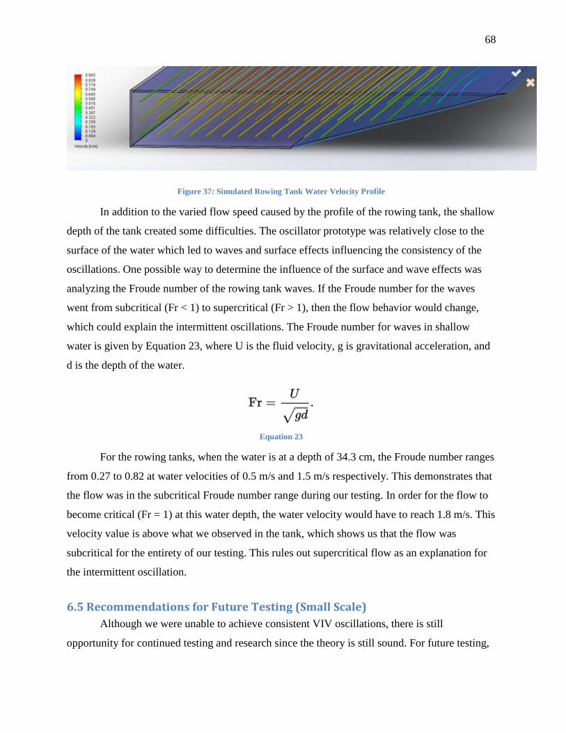
68
Figure 37: Simulated Rowing Tank Water Velocity Profile
In addition to the varied flow speed caused by the profile of the rowing tank, the shallow
depth of the tank created some difficulties. The oscillator prototype was relatively close to the
surface of the water which led to waves and surface effects influencing the consistency of the
oscillations. One possible way to determine the influence of the surface and wave effects was
analyzing the Froude number of the rowing tank waves. If the Froude number for the waves
went from subcritical (Fr < 1) to supercritical (Fr > 1), then the flow behavior would change,
which could explain the intermittent oscillations. The Froude number for waves in shallow
water is given by Equation 23, where U is the fluid velocity, g is gravitational acceleration, and
d is the depth of the water.
Equation 23
For the rowing tanks, when the water is at a depth of 34.3 cm, the Froude number ranges
from 0.27 to 0.82 at water velocities of 0.5 m/s and 1.5 m/s respectively. This demonstrates that
the flow was in the subcritical Froude number range during our testing. In order for the flow to
become critical (Fr = 1) at this water depth, the water velocity would have to reach 1.8 m/s. This
velocity value is above what we observed in the tank, which shows us that the flow was
subcritical for the entirety of our testing. This rules out supercritical flow as an explanation for
the intermittent oscillation.
6.5 Recommendations for Future Testing (Small Scale)
Although we were unable to achieve consistent VIV oscillations, there is still
opportunity for continued testing and research since the theory is still sound. For future testing,

69
there are a couple of improvements that can be made in order to increase the chances of success.
The most significant improvement moving forward would be to find a testing facility with a
more consistent flow. Our project was limited and constrained by the inconsistent flow speed,
which prevented us from fully testing the parameters of our energy harvesting design.
If a more controlled and consistent testing facility can be utilized, then there are
additional tests that can be conducted to determine the optimal piezoelectric energy harvester
system. For example, the mass of the system can be varied in order to get the natural frequency
of the device as close as possible to the vortex shedding of the water. Testing over a wider range
of water velocities can also be conducted in order to determine how large a range the
oscillations can occur in. In addition, the load resistance test that our team conducted out of the
water can be conducted in the water to truly determine the optimal load resistance.
Another parameter of the energy harvester design that can be tested is to increase the
number of piezoelectric transducers attached in series. Our design had two transducers attached
in series, but adding more, in theory, would increase the voltage produced in the system. This
would help increase the amount of power generated and could potentially increase the efficiency
of the energy harvester. However, a more secure method of attaching the piezoelectric films to
the springs should be investigated to improve durability.
6.6 Large Scale Testing and Real World Feasibility
To determine if VIV is a practical harvesting method, testing needs to be conducted on a
larger scale than the energy harvester constructed for this project. Testing on a larger scale
would allow for a better determination of how much power could actually be generated using
VIV. It would reduce the effects of variables such as friction, boundary layer effects, and erratic
flow speed which had a significant impact on the consistency of our prototype. Additionally,
increasing the scale of the project would allow for the use of more efficient electrical conversion
methods such as electromagnetic or electrostatic.
For a linear alternator, which converts linear oscillation into electrical power using
electromagnetism, the mechanical to electrical efficiency could realistically be 95% (Bard &
Kracht, 2013). Based on the 28.8% mechanical conversion efficiency measured in this project, a
device using a 95% efficient linear alternator could feasibly produce 1 kW of electrical power in
70
water flowing at 0.6 m/s. Assuming appropriate springs could be chosen based on the system
mass, this could be accomplished by using 20 cylinders with a diameter of 0.45m and a length
of 3.44m.
Large scale VIV energy harvesting has the potential to produce a greater amount of
power with more consistency than the small scale harvester used in this project. However, as the
size of the harvester increases, it has a greater impact on the environment. In order for VIV to
become an environmentally friendly hydropower alternative, the size of the harvester must be
limited, which would limit its power production.
71
References Accelerometers: Introduction to Acceleration Measurement. (2016). Omega.
American Shad. (n.d.). Retrieved October 12, 2016, from
http://www.wildlife.state.nh.us/fishing/profiles/american-shad.html
Avram, P., McKee, R., Tuzun, T., & Geiger, B. (2008). A Linear Generator Power Take-Off
System for the VIVACE Hydrokinetic Energy Converter.
Ball, I. M., Killen, T. J., Sakhuja, S., Warner, E. T., & Faculty Advisor: Savilonis, B. J. (2012).
Maximizing Vortex Induced Vibrations through Geometry Variation.
Bard, J., & Kracht, P. (2013). Report on Linear Generator Systems for Wave Energy
Converters. Structural Design of Wave Energy Generators.
Bernitsas, M. M., Ben-Simon, Y., Raghavan, K., & Garcia, E. M. (2008). The VIVACE
Converter: Model Tests at High Damping and Reynolds Number Around 105. Journal of
Offshore Mechanics and Arctic Engineering, 131(1), 011102-011102.
doi:10.1115/1.2979796
Bearman, P. W. (1984). Vortex Shedding from Oscillating Bluff Bodies. Annual Review of
Fluid Mechanics, 16(1), 195-222. doi:10.1146/annurev.fl.16.010184.001211
Boisseau, S.,Despesse, G. and Seddik, B. Ahmed. Electrostatic Conversion for Vibration
Energy Harvesting, Small-Scale Energy Harvesting, Intech, 2012.
Blevins, R. (1990). Flow-Induced Vibration. New York: Van Nostrand Reinhold.
Costanzo, I., Kelsey, A., Ogren, F., Wians, D., & Faculty Advisor: Savilonis, B. J. (2016).
Design of a Novel Concept for Harnessing Tidal Stream Power.
Distler, D. B., Johnson, B. G., Kielbasa, M. J., Phinney, B. C., & Faculty Advisor: Savilonis, B.
J. (2011). Optimization of Oscillating Body for Vortex Induced Vibrations.
Dynamometer: Introduction and Types. (2015).
Elert, G. (2002). Speed of Ocean Currents. Retrieved September 21, 2016, from
http://hypertextbook.com/facts/2002/EugeneStatnikov.shtml
Effects on the Environment. (2015). Retrieved October 12, 2016, from
http://nnmrec.oregonstate.edu/education/effects-environment
72
Environmental Impact of Wave Energy Devices. (n.d.). Retrieved October 12, 2016, from
http://www.alternative-energy-tutorials.com/energy-articles/environmental impact-of-
wave-energy.html
Flahiff, D. (2008, December 3). VIVACE: Slow Water Current Energy Mimics Schools of Fish.
Retrieved September 21, 2016, from http://inhabitat.com/vivace-vortex-hydro-energy/
Hall-Stinson, A. S., Lehrman, C. J., Tripp, E. R., & Faculty Advisor: Savilonis, B. J. (2011).
Energy Generation from Vortex Induced Vibrations.
Gabbai, R. D., & Benaroya, H. (2005). An overview of modeling and experiments of vortex-
induced vibration of circular cylinders. Journal of Sound and Vibration, 282(3–5), 575-
616. doi:http://dx.doi.org/10.1016/j.jsv.2004.04.017
Hadas, Z., Ondrusek, C., & Singule, V. (2010). Power sensitivity of vibration energy harvester.
Microsystem technologies, 16(5), 691-702.Pranita, B. A. (2016). Subsea Pipeline:
Fatigue Free Span Analysis.
Hobbs, W. B. (2010). Piezoelectric energy harvesting: vortex induced vibrations in plants, soap
films, and arrays of cylinders.
Kuhn, A. (2008, January 3). Relocated Three Gorges Residents Face Challenges. Retrieved
October 12, 2016, from
http://www.npr.org/templates/story/story.php?storyId=17784497
Measurement Specialties. “Piezo Film Sensors Technical Manual.” Retrieved from
https://www.sparkfun.com/datasheets/Sensors/Flex/MSI-techman.pdf
Measurement Specialties (2009). “DT Series Elements with Lead Attachment Data Sheet.”
Retrieved from http://www.mouser.com/ds/2/418/DT_Series_LeadAttach-709992.pdf
Mehmood, A., Abdelkefi, A., Hajj, M. R., Nayfeh, A. H., Akhtar, I., & Nuhait, A. O. (2013).
Piezoelectric energy harvesting from vortex-induced vibrations of circular cylinder.
Journal of Sound and Vibration, 332(19), 4656-4667.
doi:http://dx.doi.org/10.1016/j.jsv.2013.03.033
Modir, Alireza, Kahrom, Mohsen & Farshidianfar, Anoshirvan. Mass ratio effect on vortex
induced vibration of a flexibly mounted circular cylinder, an experimental study,
International Journal of Marine Energy, Volume 16, December 2016, Pages 1-1
Piezo Systems. “Piezoceramic Materials and Properties.” Retrieved from
http://www.piezo.com/prodmaterialprop.html
73
Principles of Strain Gauges. Kyowa.
LVDT Pressure Sensors. (2009). Sensorland.
Ledoux, A. (2011). Theory of Piezoelectric materials and their Applications in Civil
Engineering (Doctoral dissertation, Massachusetts Institute of Technology).
Maximum Power Transfer Theorem. (2015, April 21). Retrieved September 22, 2016, from
http://www.electronicshub.org/maximum-power-transfer-theorem/
See, L. (2003, June 08). Waters of Three Gorges Dam Will Wash Over World Culture.
Retrieved October 12, 2016, from http://articles.latimes.com/2003/jun/08/opinion/oe-
see8
Sherrit, S. (2008). The Physical Acoustics of Energy Harvesting. Pasadena, CA: Jet Propulsion
Labratory, California Institute of technology.
Tardiveau, R., Giraud, F., Amanci, A., Dawson, F., Giraud-Audine, C., Amberg, M., &
Lemaire-Semail, B. (2013). Power Consideration in a Piezoelectric Generator. Smart
Materials Research, 2013.
Techet, A. H. (2005). Vortex Induced Vibrations: MIT Opencourseware. Shu, Y.C., and Lien,
I.C. (2006). Analysis of Power Output for Piezoelectric Energy Harvesting Systems.
Smart Materials and Structures. 15, 1499.
The Strain Gauge. (2016). Omega.
Umans, S. D., & .. (n.d.). Fitzgerald and Kingsley's Electric Machinery.
University Communications. (2013, January 16). Hydropower Dams Hamper Migrating Fish
Despite Passage Features, Study Finds. Retrieved October 12, 2016, from
https://uanews.arizona.edu/story/hydropower-dams-hamper-migrating-fish-
despite-passage-features-study-finds
U.S. Energy Information Administration (2016). Retrieved from http://www.eia.gov/
Vortex Hydro Energy. (2016). Retrieved from http://www.vortexhydroenergy.com
Wagner, Jürgen (Self-photographed) [CC BY-SA 4.0
(http://creativecommons.org/licenses/bysa/4.0)], via Wikimedia Commons
74
Williamson, C. H. K., & Govardhan, R. (2008). A brief review of recent results in vortex-
induced vibrations. Journal of Wind Engineering and Industrial Aerodynamics, 96(6–7),
713-735. doi:http://dx.doi.org/10.1016/j.jweia.2007.06.019
Williamson, C.H.K. & Govardhan, R. (2004). Vortex-Induced Vibrations. Annual Review of
Fluid Mechanics, 36(1), 413-455. doi:doi:10.1146/annurev.fluid.36.050802.122128
Zahari, M. A., & Dol, S. S. (2014). Application of Vortex Induced Vibration Energy:
Generation Technologies to the Offshore Oil and Gas Platform: The Preliminary Study
(Vol. 8): International Journal of Mechanical, Aerospace, Industrial, Mechatronic and
Manufacturing Engineering.
Zhang, Min & Wang, Junlei, “Experimental Study on Piezoelectric Energy Harvesting from
Vortex-Induced Vibrations and Wake-Induced Vibrations,” Journal of Sensors, vol.
2016, Article ID 2673292, 7 pages, 2016. doi:10.1155/2016/2673292
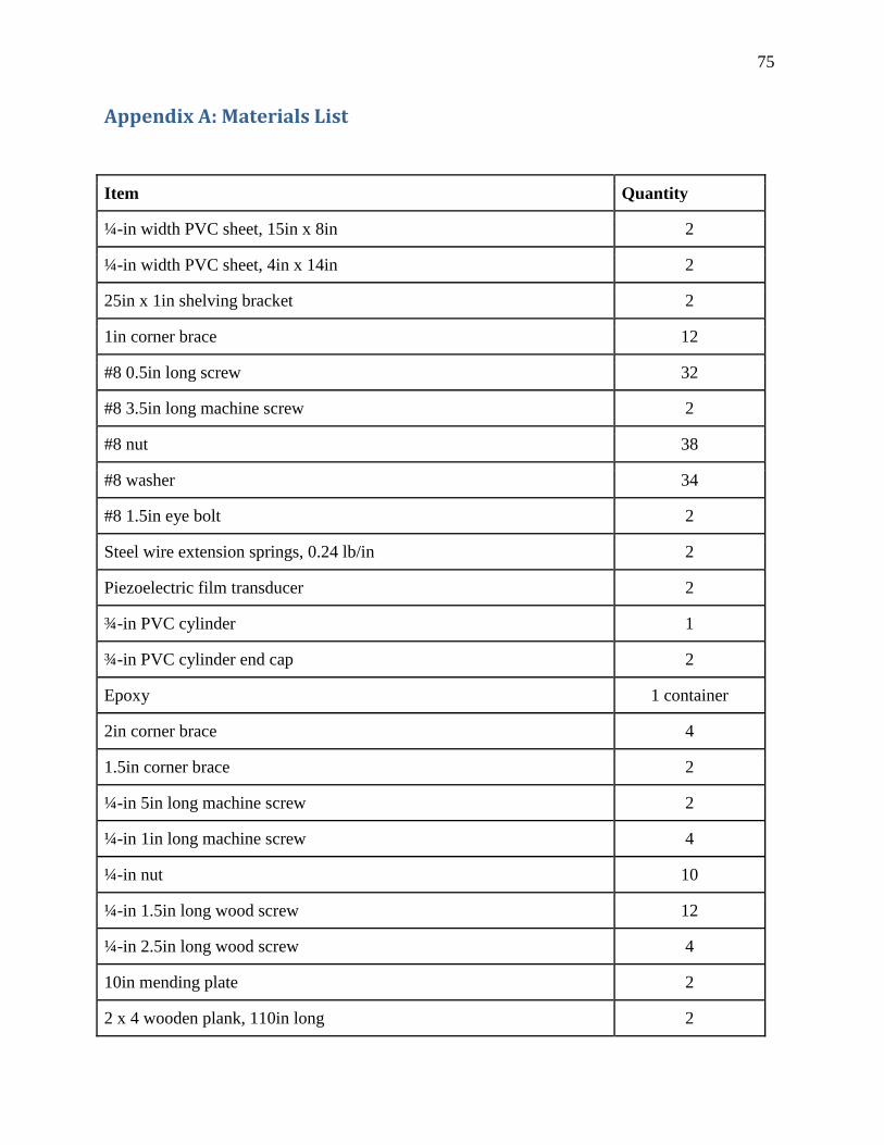
75
Appendix A: Materials List
Item Quantity
¼-in width PVC sheet, 15in x 8in 2
¼-in width PVC sheet, 4in x 14in 2
25in x 1in shelving bracket 2
1in corner brace 12
#8 0.5in long screw 32
#8 3.5in long machine screw 2
#8 nut 38
#8 washer 34
#8 1.5in eye bolt 2
Steel wire extension springs, 0.24 lb/in 2
Piezoelectric film transducer 2
¾-in PVC cylinder 1
¾-in PVC cylinder end cap 2
Epoxy 1 container
2in corner brace 4
1.5in corner brace 2
¼-in 5in long machine screw 2
¼-in 1in long machine screw 4
¼-in nut 10
¼-in 1.5in long wood screw 12
¼-in 2.5in long wood screw 4
10in mending plate 2
2 x 4 wooden plank, 110in long 2

76
Item Quantity
¼-in width PVC sheet, 15in x 8in 2
¼-in width PVC sheet, 4in x 14in 2
25in x 1in shelving bracket 2
2 x 3 wooden plank, 18in long 1

![EXPERIMENTS ON VORTEX-INDUCED VIBRATION …ijame.ump.edu.my/images/Volume_11 June 2015/31_Rahman and... · EXPERIMENTS ON VORTEX-INDUCED VIBRATION OF A VERTICAL ... Blevins [10],](https://img.pdfslide.net/doc/110x75/5b83b77d7f8b9a31608def8f/experiments-on-vortex-induced-vibration-ijameumpedumyimagesvolume11-june-201531rahman.jpg)