STATISTICAL DATA ANALYSIS WORK PLAN Coal ... DATA ANALYSIS WORK PLAN Coal Combustion Residual Rule Groundwater Monitoring System Compliance Four Corners Power Plant Fruitland, New

STATISTICAL DATA ANALYSIS WORK PLAN Coal Combustion Residual Rule Groundwater Monitoring System Compliance

Four Corners Power Plant Fruitland, New Mexico

Prepared for:

Arizona Public Service

Prepared by:

Amec Foster Wheeler Environment & Infrastructure, Inc.

Phoenix, Arizona

October 13, 2017

Project No. 14-2016-2024

Statistical Data Analysis Work Plan Coal Combustion Residual Rule Groundwater Monitoring System Compliance

TABLE OF CONTENTS Page

1.0 INTRODUCTION ............................................................................................................. 1 1.1 Objectives ............................................................................................................ 1 1.2 Purpose ............................................................................................................... 1 1.3 Conceptual Site Model ......................................................................................... 2

1.3.1 Site Description ........................................................................................ 3 1.3.2 Site Geology ............................................................................................. 4 1.3.3 Site Hydrogeology .................................................................................... 4

1.4 Monitoring System Sampling Adequacy ............................................................... 5 1.4.1 Downgradient Groundwater Monitoring Well Networks ............................. 5 1.4.2 Background Groundwater Monitoring Wells .............................................. 6

2.0 EXPLORATORY DATA ANALYSIS ................................................................................. 7 2.1 Data Evaluation Objectives .................................................................................. 8 2.2 Constituents of Concern ....................................................................................... 8 2.3 Non-Detects ......................................................................................................... 9 2.4 Stationarity ......................................................................................................... 10 2.5 Data Dependence .............................................................................................. 10

2.5.1 Quick Spatial Interpolation ...................................................................... 11 2.5.2 Autocorrelation ....................................................................................... 11 2.5.3 Time Series Analysis .............................................................................. 12

2.6 Statistical Independence .................................................................................... 13 2.6.1 Data Detrending ..................................................................................... 14 2.6.2 Data Domaining ...................................................................................... 14

2.7 Data Distributions ............................................................................................... 15 2.8 Outlier Tests ...................................................................................................... 16

3.0 DETECTION MONITORING .......................................................................................... 16 3.1 Data Evaluation Objectives ................................................................................ 17 3.2 Constituents of Concern ..................................................................................... 17 3.3 Background Comparison Tests .......................................................................... 17

3.3.1 Interwell versus Intrawell Comparisons .................................................. 17 3.3.2 Upper Prediction Limits .......................................................................... 18

3.4 Performance Standards ..................................................................................... 18 4.0 RECOMMENDATIONS FOR FUTURE EVALUATIONS ................................................ 19 5.0 SOFTWARE .................................................................................................................. 20 6.0 CERTIFICATION ........................................................................................................... 21 7.0 REFERENCES .............................................................................................................. 22

LIST OF TABLES

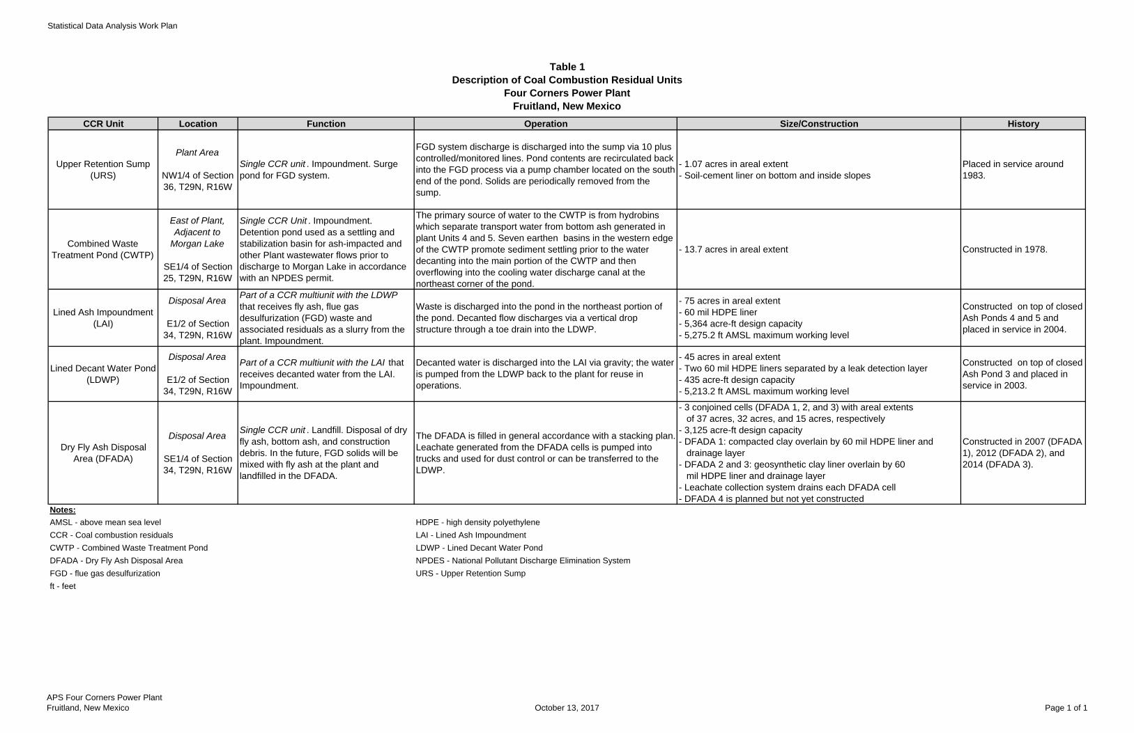
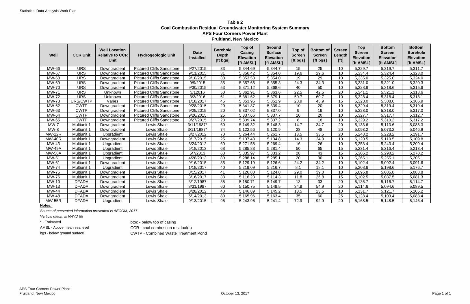
Table 1 Description of Coal Combustion Residual Units Table 2 Coal Combustion Residual Groundwater Monitoring System Summary

LIST OF FIGURES Figure 1 Site Location Map Figure 2 CCR Units and Monitoring System Summary

APS Four Corners Power Plant Fruitland, New Mexico October 13, 2017 Page i


LIST OF ACRONYMS AND ABBREVIATIONS

% percent § Section AMSL above mean sea level APS Arizona Public Service CCR coal combustion residuals CFR Code of Federal Regulations CSM Conceptual Site Model CWTP Combined Waste Treatment Pond DFADA Dry Fly Ash Disposal Area EDA exploratory data analysis FCPP Four Corners Power Plant ft foot, feet LAI Lined Ash Impoundment LDWP Lined Decant Water Pond Multiunit 1 CCR multiunit comprised of LAI and LDWP RL reporting limit ROS regression order on statistics SDAWP Statistical Data Analysis Work Plan SWFPR site-wide false positive rate UPL(s) upper prediction limit(s) URS Upper Retention Sump TDS total dissolved solids VSP Visual Sampling Plan

USEPA United States Environmental Protection Agency

APS Four Corners Power Plant Fruitland, New Mexico October 13, 2017 Page ii


1.0 INTRODUCTION

This Statistical Data Analysis Work Plan (SDAWP) was prepared by Amec Foster Wheeler Environment & Infrastructure, Inc. on behalf of Arizona Public Service (APS) for the Four Corners Power Plant (FCPP) located in Fruitland, New Mexico. The SDAWP details the scope and implementation of statistical criteria and procedures to evaluate site data in accordance with Coal Combustion Residuals (CCR) groundwater monitoring requirements detailed in 40 Code of Federal Regulations (CFR) Sections (§) 257.90 through 257.95 (herein referred to as the CCR Rule) (Federal Register, 2015).

1.1 Objectives

The SDAWP will serve as a reference document throughout the FCPP CCR groundwater monitoring program to:

• assess adequacy of sampled data to service statistical procedures (Sections 1.0 and 2.0);

• select appropriate statistical methods for each constituent in each monitoring well (Sections 2.0 and 3.0);

• develop background constituent decision threshold statistics (Section 3.0);

• identify statistically significant increases in constituent concentrations over background (Section 3.0); and

• indicate how evaluations of future data will be conducted in the case that a statistically significant increase over background is detected (Section 4.0).

1.2 Purpose

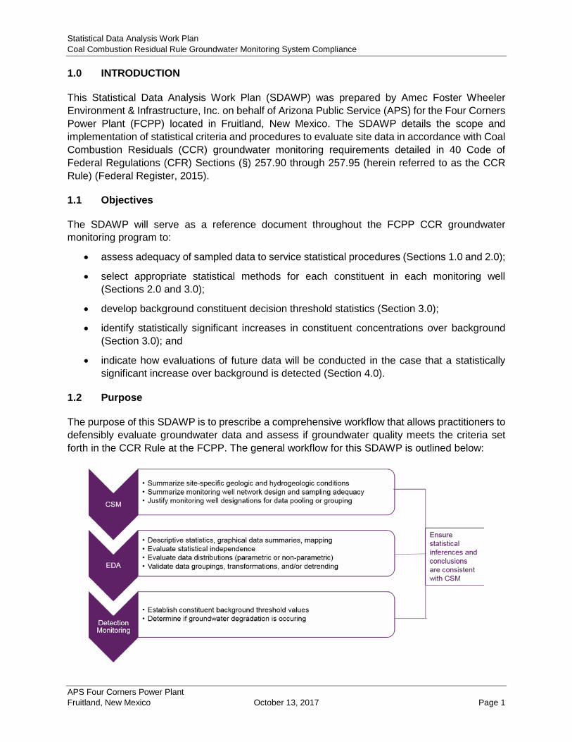
The purpose of this SDAWP is to prescribe a comprehensive workflow that allows practitioners to defensibly evaluate groundwater data and assess if groundwater quality meets the criteria set forth in the CCR Rule at the FCPP. The general workflow for this SDAWP is outlined below:

APS Four Corners Power Plant Fruitland, New Mexico October 13, 2017 Page 1


1.3 Conceptual Site Model

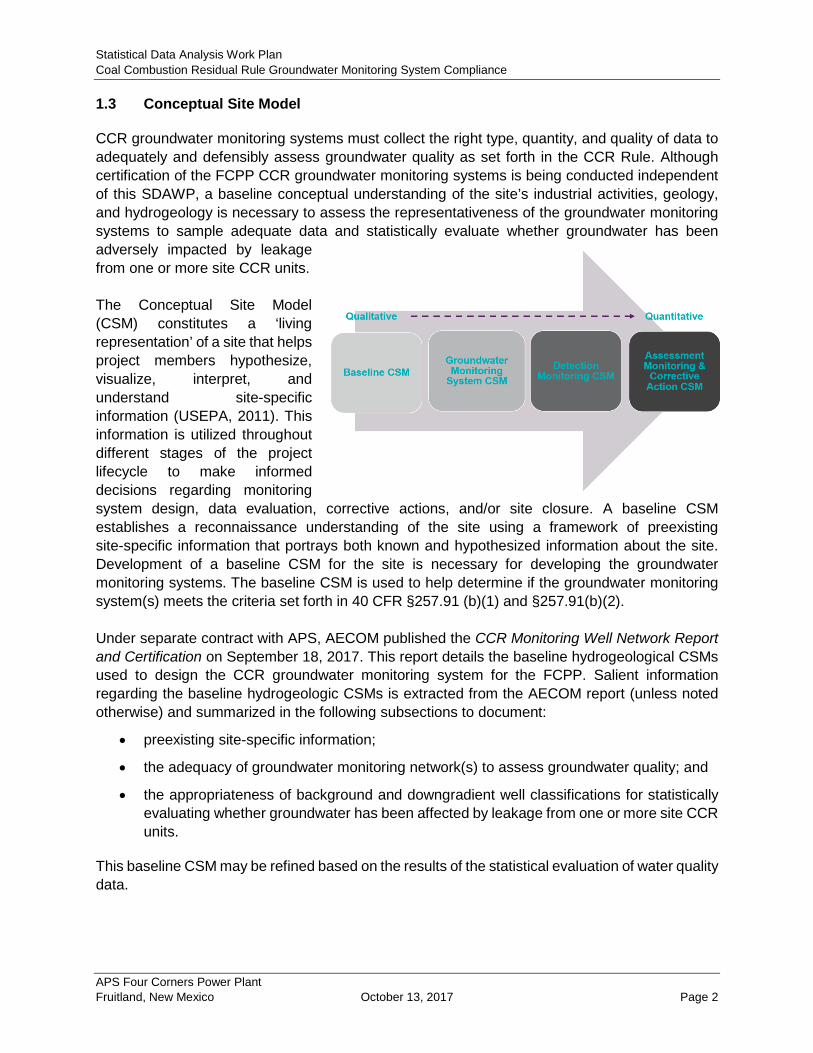
CCR groundwater monitoring systems must collect the right type, quantity, and quality of data to adequately and defensibly assess groundwater quality as set forth in the CCR Rule. Although certification of the FCPP CCR groundwater monitoring systems is being conducted independent of this SDAWP, a baseline conceptual understanding of the site’s industrial activities, geology, and hydrogeology is necessary to assess the representativeness of the groundwater monitoring systems to sample adequate data and statistically evaluate whether groundwater has been adversely impacted by leakage from one or more site CCR units. The Conceptual Site Model (CSM) constitutes a ‘living representation’ of a site that helps project members hypothesize, visualize, interpret, and understand site-specific information (USEPA, 2011). This information is utilized throughout different stages of the project lifecycle to make informed decisions regarding monitoring system design, data evaluation, corrective actions, and/or site closure. A baseline CSM establishes a reconnaissance understanding of the site using a framework of preexisting site-specific information that portrays both known and hypothesized information about the site. Development of a baseline CSM for the site is necessary for developing the groundwater monitoring systems. The baseline CSM is used to help determine if the groundwater monitoring system(s) meets the criteria set forth in 40 CFR §257.91 (b)(1) and §257.91(b)(2). Under separate contract with APS, AECOM published the CCR Monitoring Well Network Report and Certification on September 18, 2017. This report details the baseline hydrogeological CSMs used to design the CCR groundwater monitoring system for the FCPP. Salient information regarding the baseline hydrogeologic CSMs is extracted from the AECOM report (unless noted otherwise) and summarized in the following subsections to document:

• preexisting site-specific information;

• the adequacy of groundwater monitoring network(s) to assess groundwater quality; and

• the appropriateness of background and downgradient well classifications for statistically evaluating whether groundwater has been affected by leakage from one or more site CCR units.

This baseline CSM may be refined based on the results of the statistical evaluation of water quality data.



1.3.1 Site Description

The site setting is as follows:

• FCPP is an operating power plant owned by APS and four other utilities:

− FCPP burns low sulfur coal in two electrical generating units (Units 4 and 5) and has a net generating capacity of 1,540 megawatts.

− Coal burned at the plant is generally sourced from the nearby Navajo Mine (Navajo Transitional Energy Company, 2016).

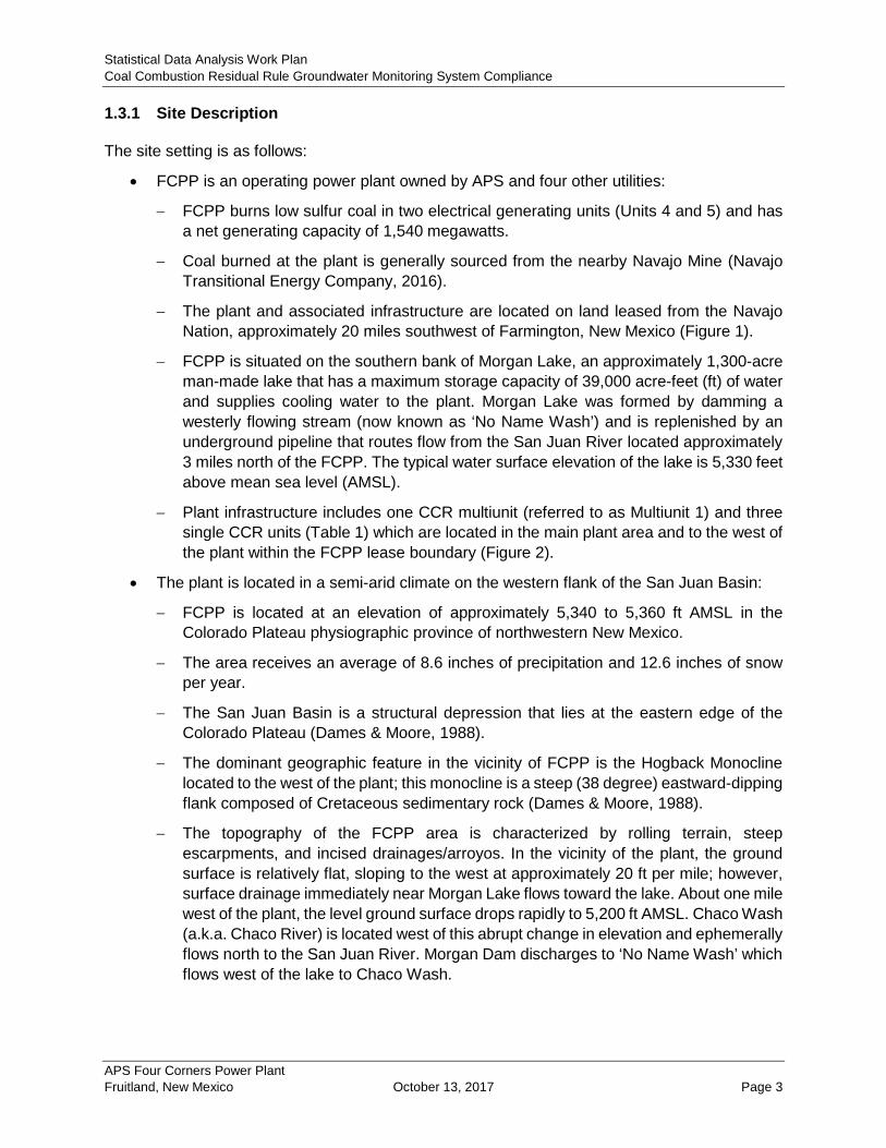
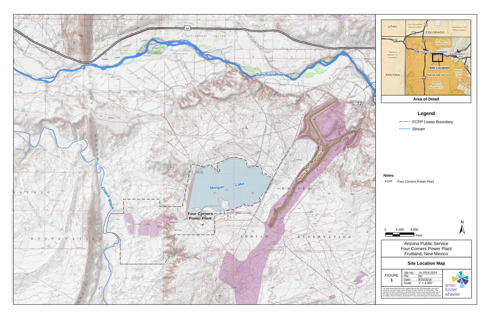
− The plant and associated infrastructure are located on land leased from the Navajo Nation, approximately 20 miles southwest of Farmington, New Mexico (Figure 1).

− FCPP is situated on the southern bank of Morgan Lake, an approximately 1,300-acre man-made lake that has a maximum storage capacity of 39,000 acre-feet (ft) of water and supplies cooling water to the plant. Morgan Lake was formed by damming a westerly flowing stream (now known as ‘No Name Wash’) and is replenished by an underground pipeline that routes flow from the San Juan River located approximately 3 miles north of the FCPP. The typical water surface elevation of the lake is 5,330 feet above mean sea level (AMSL).

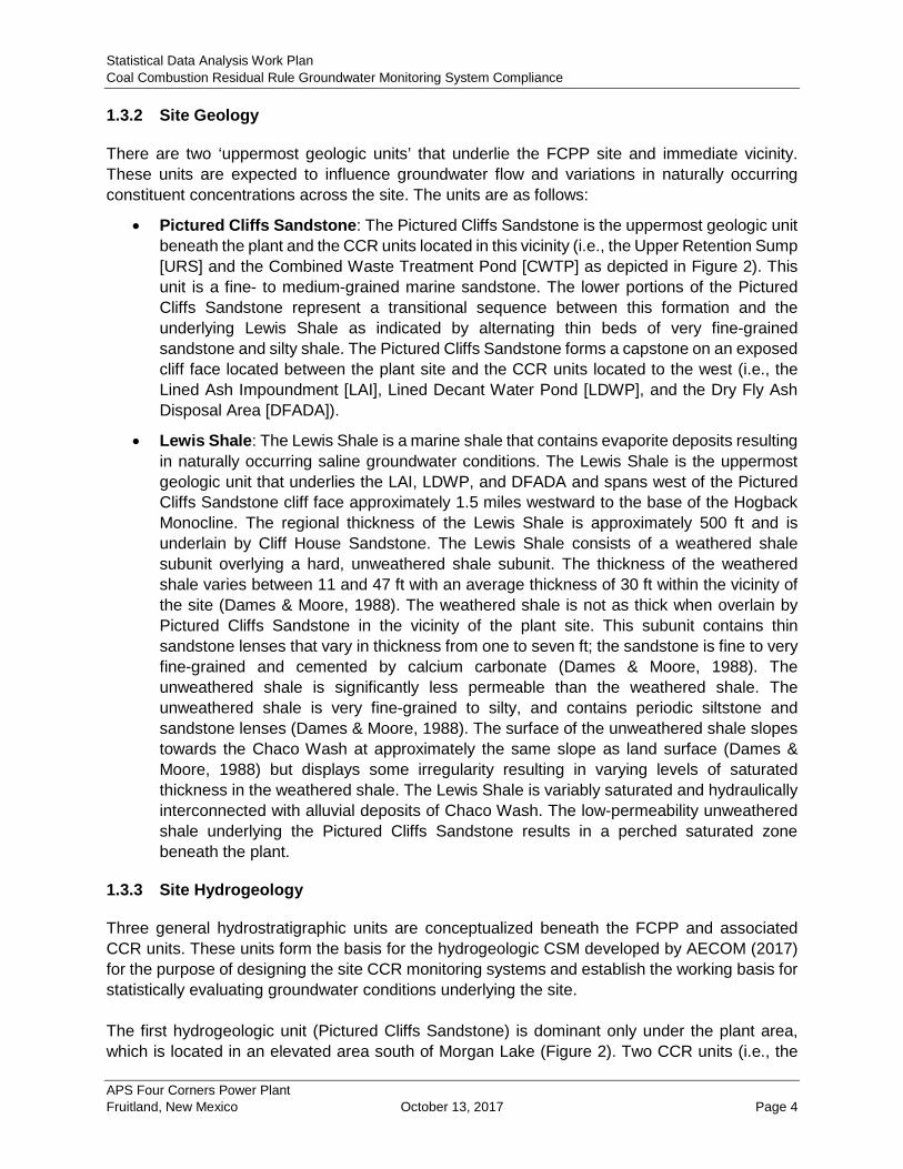
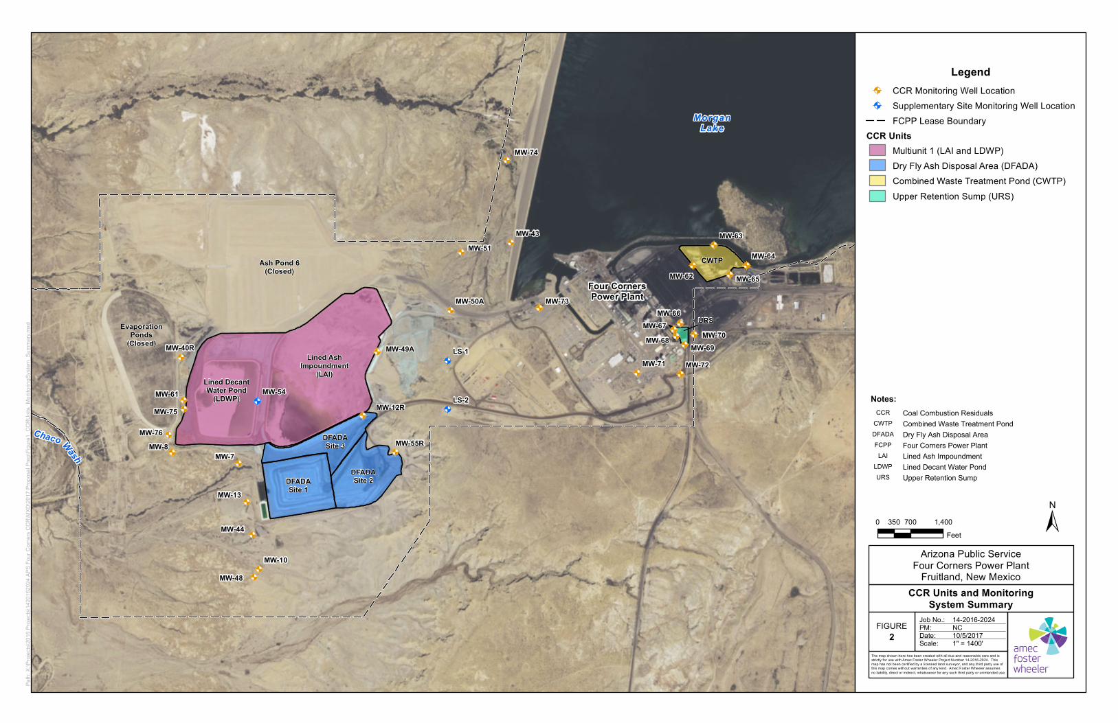
− Plant infrastructure includes one CCR multiunit (referred to as Multiunit 1) and three single CCR units (Table 1) which are located in the main plant area and to the west of the plant within the FCPP lease boundary (Figure 2).

• The plant is located in a semi-arid climate on the western flank of the San Juan Basin:

− FCPP is located at an elevation of approximately 5,340 to 5,360 ft AMSL in the Colorado Plateau physiographic province of northwestern New Mexico.

− The area receives an average of 8.6 inches of precipitation and 12.6 inches of snow per year.

− The San Juan Basin is a structural depression that lies at the eastern edge of the Colorado Plateau (Dames & Moore, 1988).

− The dominant geographic feature in the vicinity of FCPP is the Hogback Monocline located to the west of the plant; this monocline is a steep (38 degree) eastward-dipping flank composed of Cretaceous sedimentary rock (Dames & Moore, 1988).

− The topography of the FCPP area is characterized by rolling terrain, steep escarpments, and incised drainages/arroyos. In the vicinity of the plant, the ground surface is relatively flat, sloping to the west at approximately 20 ft per mile; however, surface drainage immediately near Morgan Lake flows toward the lake. About one mile west of the plant, the level ground surface drops rapidly to 5,200 ft AMSL. Chaco Wash (a.k.a. Chaco River) is located west of this abrupt change in elevation and ephemerally flows north to the San Juan River. Morgan Dam discharges to ‘No Name Wash’ which flows west of the lake to Chaco Wash.



1.3.2 Site Geology

There are two ‘uppermost geologic units’ that underlie the FCPP site and immediate vicinity. These units are expected to influence groundwater flow and variations in naturally occurring constituent concentrations across the site. The units are as follows:

• Pictured Cliffs Sandstone: The Pictured Cliffs Sandstone is the uppermost geologic unit beneath the plant and the CCR units located in this vicinity (i.e., the Upper Retention Sump [URS] and the Combined Waste Treatment Pond [CWTP] as depicted in Figure 2). This unit is a fine- to medium-grained marine sandstone. The lower portions of the Pictured Cliffs Sandstone represent a transitional sequence between this formation and the underlying Lewis Shale as indicated by alternating thin beds of very fine-grained sandstone and silty shale. The Pictured Cliffs Sandstone forms a capstone on an exposed cliff face located between the plant site and the CCR units located to the west (i.e., the Lined Ash Impoundment [LAI], Lined Decant Water Pond [LDWP], and the Dry Fly Ash Disposal Area [DFADA]).

• Lewis Shale: The Lewis Shale is a marine shale that contains evaporite deposits resulting in naturally occurring saline groundwater conditions. The Lewis Shale is the uppermost geologic unit that underlies the LAI, LDWP, and DFADA and spans west of the Pictured Cliffs Sandstone cliff face approximately 1.5 miles westward to the base of the Hogback Monocline. The regional thickness of the Lewis Shale is approximately 500 ft and is underlain by Cliff House Sandstone. The Lewis Shale consists of a weathered shale subunit overlying a hard, unweathered shale subunit. The thickness of the weathered shale varies between 11 and 47 ft with an average thickness of 30 ft within the vicinity of the site (Dames & Moore, 1988). The weathered shale is not as thick when overlain by Pictured Cliffs Sandstone in the vicinity of the plant site. This subunit contains thin sandstone lenses that vary in thickness from one to seven ft; the sandstone is fine to very fine-grained and cemented by calcium carbonate (Dames & Moore, 1988). The unweathered shale is significantly less permeable than the weathered shale. The unweathered shale is very fine-grained to silty, and contains periodic siltstone and sandstone lenses (Dames & Moore, 1988). The surface of the unweathered shale slopes towards the Chaco Wash at approximately the same slope as land surface (Dames & Moore, 1988) but displays some irregularity resulting in varying levels of saturated thickness in the weathered shale. The Lewis Shale is variably saturated and hydraulically interconnected with alluvial deposits of Chaco Wash. The low-permeability unweathered shale underlying the Pictured Cliffs Sandstone results in a perched saturated zone beneath the plant.

1.3.3 Site Hydrogeology

Three general hydrostratigraphic units are conceptualized beneath the FCPP and associated CCR units. These units form the basis for the hydrogeologic CSM developed by AECOM (2017) for the purpose of designing the site CCR monitoring systems and establish the working basis for statistically evaluating groundwater conditions underlying the site. The first hydrogeologic unit (Pictured Cliffs Sandstone) is dominant only under the plant area, which is located in an elevated area south of Morgan Lake (Figure 2). Two CCR units (i.e., the



URS and CWTP) reside within this area. The Pictured Cliffs Sandstone is the uppermost water bearing unit for the plant area and extends from ground surface (between approximately 5,340 to 5,360 ft AMSL) to approximately 5,300 ft AMSL in the plant area. Groundwater in this area is strongly influenced by Morgan Lake (at a surface elevation of approximately 5,330 ft AMSL) and generally flows northward towards the lake. However, construction and operations of the plant have resulted in disturbed ground conditions and associated impacts are not well understood. This uncertainty will be considered when interpreting constituent concentrations and any potential impact on adequacy of background well locations. The second hydrogeologic unit (Weathered Lewis Shale/Alluvium) underlies the Pictured Cliffs Sandstone in the plant area and the Multiunit 1 and the DFADA CCR units (Figure 2) in the disposal area, approximately 1 mile west of the plant. The weathered Lewis Shale and the hydraulically connected alluvial deposits along Chaco Wash are designated as the uppermost water bearing unit in the disposal area. Although the Lewis Shale is geologically continuous in this area, it is unsaturated in the vicinity of the DFADA. The water table in the weathered Lewis Shale can exhibit local seasonal fluctuations that are attributed to interactions between rates of groundwater recharge and discharge (Dames & Moore, 1988) from/to Morgan Lake, historical unlined ponds, and Chaco Wash. Groundwater flow generally follows the surface topography and descends to the west-southwest in the disposal area, mainly in the weathered shale and in local alluvial channels that drain toward the Chaco Wash (APS, 2013). The third hydrogeologic unit (Unweathered Lewis Shale) consists of the unweathered Lewis Shale and is a regionally extensive confining unit that forms the base of the uppermost aquifers in the plant and disposal areas.

1.4 Monitoring System Sampling Adequacy

Multiple monitoring well systems are in place at the FCPP to monitor groundwater conditions beneath the four site CCR units. The installation of these networks is summarized in the CCR Monitoring Well Network Report and Certification and is identified as compliant with 40 CFR §257.91(a) through (e) (AECOM, 2017). AECOM also prepared Sampling and Analysis Plan, Coal Combustion Residual (CCR) Groundwater Monitoring (2015) to document the methods and procedures used to conduct groundwater sampling and evaluate potential impacts of site CCR units. Sampling coverage and adequacy of the CCR monitoring well networks to facilitate the statistical evaluations detailed in this SDAWP are discussed in the following subsections.

1.4.1 Downgradient Groundwater Monitoring Well Networks

A total of 18 downgradient wells are in place at the site to monitor the downgradient groundwater conditions of each CCR unit (Table 2). Nine of these monitoring wells are installed in the Lewis Shale. The remaining nine other wells are completed in the Pictured Cliffs Sandstone. These wells are grouped by respective CCR unit, as described below:

• URS Downgradient Wells (Pictured Cliffs Sandstone): The groundwater flow direction underlying the URS is radially outward from the CCR unit. On this basis, five wells, MW-66, MW-67, MW-68, MW-69, and MW-70 were installed around the perimeter of the URS. Each of these wells are screened within the Pictured Cliffs Sandstone. The grouping of



monitoring wells, spatial density, and coverage of the monitoring well network are assumed representative and adequate until proven otherwise.

• CWTP Downgradient Wells (Pictured Cliffs Sandstone): Similar to the URS, the groundwater flow direction underlying the CWTP is radially outward from the CCR unit. Four monitoring wells, including MW-62, MW-63, MW-64, and MW-65, were installed around the perimeter of the CWTP. Each of these wells are screened within the Pictured Cliffs Sandstone. The grouping of monitoring wells, spatial density, and coverage of the monitoring well network are assumed representative and adequate until proven otherwise.

• Multiunit 1 Downgradient Wells (Weathered Lewis Shale/Alluvium): Six downgradient monitoring wells are in place below the toe of the western to southwestern edge of Multiunit 1: MW-7, MW-8, MW-40R, MW-61, MW-75 and MW-76 (Figure 2). Two wells, MW-40R and MW-76, are routinely either dry or have a limited saturated thickness which precludes sampling; the wells are included in the program in case conditions change in the future. The grouping of monitoring wells, spatial density, and coverage of the monitoring well network are assumed representative and adequate until proven otherwise. The screened interval for each well resides within the Weathered Lewis Shale/Alluvium.

• DFADA Downgradient Wells (Weathered Lewis Shale/Alluvium): Four existing wells are identified downgradient of the DFADA: MW-13, MW-44, MW-10 and MW-48. Each well, except MW-48, is screened within the Weathered Lewis Shale/Alluvium. The screened interval for MW-48 resides within the Unweathered Lewis Shale. The downgradient DFADA wells are known to be dry; this groundwater monitoring system was designed to detect releases since the next underlying aquifer (in the Cliff House Sandstone) is separated from the CCR unit by several hundred feet of Lewis Shale, a regional aquitard. The grouping of monitoring wells, spatial density, and coverage of the monitoring well network are assumed representative and adequate until proven otherwise.

1.4.2 Background Groundwater Monitoring Wells

The purpose of comparison statistical tests is to assess if groundwater conditions downgradient of the CCR unit indicates a potential impact from leakage. Therefore, it is important to adequately establish background conditions that accurately represent the quality of groundwater that has not been affected by leakage from a CCR unit (40 CFR §257.91). Per the CCR Monitoring Well Network Report and Certification, the following monitoring wells are designated as “background monitoring wells” for the respective geologic and hydrogeologic conditions underlying the FCPP (AECOM, 2017):

• Background Wells for the Pictured Cliffs Sandstone: Three wells (MW-71, MW-72, and MW-73) were installed to assess background groundwater quality for both the URS and the CWTP overlying the Pictured Cliffs Sandstone. Groundwater elevation data collected from 2015 to 2017 suggest that MW-71 and MW-72 may be influenced by mounding under the URS and therefore may not be representative of background. The grouping and adequacy of these background wells to assess background water quality in the Pictured Cliffs Sandstone is considered adequate until proven otherwise by the statistical procedures detailed within the SDAWP.



• Background Wells for the Weathered Lewis Shale/Alluvium: Five existing wells upgradient of Multiunit 1 and the DFADA, including MW-12R, MW-49A, MW-51, MW-50A, and MW-43, and two new wells, MW-55R and MW-74, are designated to assess background groundwater quality for Weathered Lewis Shale/Alluvium. Two of these wells could be potentially impacted by water from Multiunit 1 or the DFADA (MW-12R and MW-49A) based on their spatial proximity to the units (AECOM, 2017). Four wells, MW-43, MW-50A, MW-51, and MW-55R, are routinely either dry or have a limited saturated thickness which precludes sampling; the wells are included in the program in case conditions change in the future. The grouping and adequacy of these background wells to assess background water quality in the weathered Lewis Shale is considered adequate until proven otherwise by the statistical procedures detailed within the SDAWP.

Background can be established by a single monitoring well or a group of monitoring wells. If a group of monitoring wells are used, these wells should be screened within the same lithologic unit, exhibit similar groundwater chemistry, illustrate similar statistical merits, and be supported by the CSM. Due to the natural heterogeneity of the geologic and hydrogeologic conditions underlying the FCPP, background constituent concentrations are expected to be spatially heterogeneic across the site. The site is also expected to exhibit temporal heterogeneity due to local climatic regimes, potential leakage from Morgan Lake, and potential operational activity at the site. The groundwater monitoring well networks, respective to sampling coverage and frequency, is assumed representative and adequate of this spatial and temporal heterogeneity until proven otherwise. The adequacy of designated background monitoring wells will be assessed using groundwater elevation data, boron data, a working understanding of the spatial heterogeneity of geochemistry underlying the FCPP, and statistical merits of constituents of concern. Historic groundwater chemistry data will be consulted during this evaluation but data preceding December 2011 will not be considered due to noted “matrix interference issues associated with saline waters” in samples analyzed prior to this date (APS, 2013). 2.0 EXPLORATORY DATA ANALYSIS

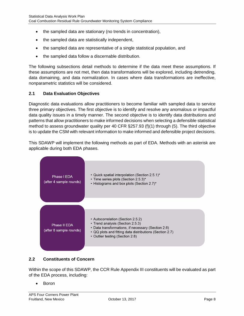
Exploratory Data Analysis (EDA) is a diagnostic data evaluation step to assess the groundwater monitoring system’s ability to collect the right quantity, quality, and type of data to adequately perform the statistical analyses set forth in 40 CFR §257.93. EDA occurs iteratively during the data evaluation process. Two phases of EDA will occur within the scope of this SDAWP. Phase I EDA will occur after completing the first four rounds of sampling and will serve as a data screening step used to inform the data collection process. The second EDA phase will occur after the first eight rounds of sampling are complete. Phase II EDA phase will service two objectives: 1) ensure the correct statistical method will be selected for determining background concentrations and performing statistical comparisons and 2) evaluate if the data meet the statistical inferences and criteria required to establish background threshold values and perform statistical comparisons.

In general, these inferences and criteria include:



• the sampled data are stationary (no trends in concentration),

• the sampled data are statistically independent,

• the sampled data are representative of a single statistical population, and

• the sampled data follow a discernable distribution.

The following subsections detail methods to determine if the data meet these assumptions. If these assumptions are not met, then data transformations will be explored, including detrending, data domaining, and data normalization. In cases where data transformations are ineffective, nonparametric statistics will be considered.

2.1 Data Evaluation Objectives

Diagnostic data evaluations allow practitioners to become familiar with sampled data to service three primary objectives. The first objective is to identify and resolve any anomalous or impactful data quality issues in a timely manner. The second objective is to identify data distributions and patterns that allow practitioners to make informed decisions when selecting a defensible statistical method to assess groundwater quality per 40 CFR §257.93 (f)(1) through (5). The third objective is to update the CSM with relevant information to make informed and defensible project decisions. This SDAWP will implement the following methods as part of EDA. Methods with an asterisk are applicable during both EDA phases.

2.2 Constituents of Concern

Within the scope of this SDAWP, the CCR Rule Appendix III constituents will be evaluated as part of the EDA process, including:

• Boron



• Calcium

• Chloride

• Fluoride

• pH

• Sulfate

• Total dissolved solids (TDS)

In addition to the Appendix III constituents, groundwater elevation will also be assessed during EDA. Groundwater elevation, TDS, and boron will hold particular emphasis in assessing the adequacy of background well classifications.

2.3 Non-Detects

Non-detects, also known as left-censored measurements, are values that cannot be quantified according to the laboratory method. There are several approaches for numerically representing non-detect data to complete the data evaluations listed within this SDAWP. For the purpose of this SDAWP, simple substitution and censor estimation techniques will be used to numerically represent non-detects. These methods will be selected according to sample size, frequency of detection, and method of data evaluation. Simple substitution and censor estimation techniques are described below. Simple substitution is imputation using a qualitatively-derived value, usually equal to the reporting limit (RL), half the RL, zero, or method detection limit for a non-detect measurement. The RL represents the lowest level that can be reported by a laboratory. For simple substitution, half the RL will be used if the concentration is undetected (“U” qualifier flag) or if samples are reported as detected but not quantified. Half the RL is assumed to be between zero and the RL, which reflects the maximum likelihood estimate of the mean or median of values uniformly distributed along the interval (i.e. 0 to the RL) (USEPA, 2009). Non-detects that are estimated (“J” qualifier flag) will respect the estimated value as a valid measurement (USEPA, 2009) for statistical purposes. For traditional statistical methods, simple substitution will be considered when the frequency of detection is less than 15 percent (%) (USEPA, 2009) and the sample number is fewer than eight. Censor estimation techniques rely on modeling the underlying data distribution to quantitatively model or estimate values for non-detect measurements. These techniques attempt to fit a sample to a known distribution using a censored estimation method, such as the Kaplan-Meier estimator or the robust regression on order statistics (ROS) (USEPA, 2009) and generate a model-based estimate of statistical moments or imputed number. Parametric statistical calculations are then performed using these model-based estimates or imputations. Parametric and nonparametric statistical methods are discussed in more detail in Section 2.7. For traditional statistical methods, censor estimation techniques will be implemented when the sample number is sufficient to discern the underlying data distribution (e.g. normal, lognormal, gamma), the frequency of non-detects are between approximately 10% and 70%, and the sample number is eight or more.



In cases where more than one RL is used, ROS will be preferred. Instances where the data do not conform to a discernable data distribution nor fit the criteria set forth in this section, nonparametric statistical methods will be pursued. Substitution methods will be constituent and method dependent. Imputation for geospatial, geostatistical, and time series analyses (Section 2.5) will conform to the simple substitution criteria detailed herein. Imputation for establishing background constituent concentrations and performing statistical comparisons will favor censor estimation techniques, where appropriate, and conform to the criteria set forth in this section.

2.4 Stationarity

In the most basic sense, a stationary data set exhibits a mean with no systematic change in space or time. There are various degrees of stationarity based on the strictness of assumptions as they relate to different statistical moments (e.g. mean and variance, for example). Discussing these statistical nuances are beyond the scope of this SDAWP. El Kadi (1995) and ITRC-GRO (2016) provide a good overview of stationarity and non-stationarity in the context of groundwater statistics. For the purpose of this SDAWP, a data set that exhibits a statistical mean that changes systematically in space or time is considered non-stationary (i.e., has a trend). This change can take the form of a linear or non-linear increase or decrease in a constituent concentration in space and/or over time. The presence of a trend will automatically infer two things:

1. the sample data are statistically dependent because the trend itself demonstrates that samples exhibit a distinct relationship in space or time; and

2. the sample data set possibly exhibits more than one statistical population.

In such cases, data detrending (Section 2.6.1) and/or data domaining (Section 2.6.2) methods will be considered to transform a non-stationary data set to one that is stationary.

2.5 Data Dependence

Environmental parameters and processes inherently influence the distribution, fate, and residence of constituents. These parameters and processes are oftentimes correlated in space and/or time, meaning sample data are not completely independent and exhibit some degree of spatial and/or temporal dependence, or correlation. Spatial and temporal EDA methods allow practitioners to evaluate spatial and/or temporal relationships, such as spatial distributions and temporal trends in constituents over space and time. These methods are critical for visualizing data and further developing the CSM in terms of screening relationships between groundwater quality, geology, groundwater gradients, and seasonal trends. The following sections discuss EDA approaches in more detail by identifying their applicability and the selected methods for this SDAWP.



2.5.1 Quick Spatial Interpolation

Application: Quick spatial interpolation screens for:

• spatial anomalies, dependence, and extents of constituent concentrations in groundwater;

• spatial associations between constituent concentrations and groundwater elevation; and

• changes in spatial groundwater gradients and CCR Rule Appendix III constituent concentrations over time and any potential anomalous data that may warrant further investigation or sampling.

EDA scope: Phase I and Phase II EDA Selected methods: Selected methods include natural neighbor, inverse distance weighted, splines (or other higher order polynomials), and/or nearest neighbor. Interpolation is a generic term representing various methods used to generate maps, or spatial estimates of sampled data in unsampled locations. The quick interpolation methods listed herein are exact interpolators that do not make any assumptions regarding the distribution of the sampled data and require limited parameter input(s). An exact interpolator is one that assumes there is no error in the sampled data. More than one quick interpolation method may be selected to test the sensitivity of another quick interpolation method. An adequate number and spacing of monitoring wells are necessary to map groundwater constituent concentrations. To facilitate meaningful mapping of groundwater constituents, monitoring wells assigned to each CCR monitoring system, in addition to geologically and hydrogeologically relevant FCPP monitoring wells not identified within the CCR monitoring systems, will be considered for quick spatial interpolation. Quick interpolation maps of constituent concentrations and groundwater gradients will be integrated into the project CSM.

2.5.2 Autocorrelation

Application: Autocorrelation is used to:

• model and quantify the degree of spatial and/or temporal correlation between sampled data; and

• optimize sampling frequency and monitoring network performance.

EDA scope: Phase II EDA Selected methods: Selected methods include the variogram model and lag plot. Data dependence will be screened using quick interpolation methods. Data dependence will be quantified and tested using autocorrelation methods.



Autocorrelation quantifies the ability for a measured property, or constituent, to relate to itself in space or time. This notion follows Tolber’s first law of geography, which states that “everything is related to everything else, but near things are more related than distant things.” If a sampled constituent relates to itself in space or time it is considered to be spatially and/or temporally dependent. Autocorrelation is a valuable data evaluation tool for quantifying the presence of spatial and temporal correlations (trends and patterns) in sampled data, which is necessary to meet the criteria and assumptions for establishing background threshold values and performing statistical comparisons (Section 3.3). Within the scope of this SDAWP, standard methods to quantify autocorrelation include the variogram or lag plot (USEPA, 2009). A lag plot is a useful EDA tool to screen for non-random (e.g. autocorrelated) variation in a sampled data set. If a data set exhibits spatial or temporal autocorrelation a pattern will appear in the lag plot. The variogram model is useful for assessing sampling adequacy and autocorrelation. The variogram quantifies the ratio of dependent versus independent variation in the sampled data. This ratio is known as the nugget:sill ratio. If the nugget:sill ratio is less than 0.50, the data will be considered spatially or temporally dependent. A variogram model fits a range value to the sample data that represents the extent a sample parameter, or constituent, exhibits autocorrelation. The range can represent a distance value when modelling spatial data or a temporal frequency when modeling temporal data. The range value quantifies the distance or frequency over which a sampled property, or constituent, is considered autocorrelated. The range of autocorrelation can be useful for making informed data-driven decisions including how to best transform a spatial or temporal data set, and optimize sampling frequencies within the groundwater monitoring system(s) to ensure sample independence (Section 2.6). Therefore, optimizing sampling frequencies will minimize sampling redundancies (e.g. autocorrelation) and cost without jeopardizing sampling adequacy (40 CFR §257.94(d)(2)). The variogram requires that the data meet the assumption of intrinsic stationary, which satisfies the following criteria: the data are stationary (no systematic change in the mean) and the variance depends only on sample separation increment, or separation distance between samples in space or time. Ideally, shorter separation increments will illustrate a higher degree of autocorrelation whereas larger separation increments will exhibit lower degrees of autocorrelation, which follows the principle of Tobler’s First Law of Geography.

2.5.3 Time Series Analysis

Application: Time series analysis is used to:

• screen for potential anomalous data that warrant further investigation;

• screen for temporal trends in constituent concentrations in each monitoring well; and

• test for significance of temporal trends, where identified.

EDA scope: Phase I and Phase II EDA



Selected methods: Selected methods include time series plots and parametric and non-parametric trend analysis. A time series is a sample data set ordered consecutively by sample date. Plotting constituent concentrations as a time series provides a very quick visual approach to screen monitoring well data for potential outliers and/or temporal trends. In this case, outliers will consist of visually identifying constituent concentrations that do not conform to the historic temporal variations characteristic to a given well, such as extremely high or low concentration values. Long-term temporal trends exist when a constituent time series shows a discernable pattern of increase or decrease in constituent concentrations over time, thereby indicating that the sample mean is non-stationary over time. The significance and slope of these trends will be evaluated using the Mann-Kendall and the Theil-Sen tests to determine if the increase or decrease in constituent concentrations are significant (p < 0.05). The Mann-Kendall and the Theil-Sen tests make no assumptions regarding the data distribution. The Mann-Kendall test does not indicate the slope of the trend, which is a shortcoming for this method. The Theil-Sen test can be used in conjunction with the Mann-Kendall test to assess the magnitude of the slope of the trend. If trends are statistically and hydrogeologically justified, the data should be detrended (Section 2.6.1) prior to establishing background threshold values. If data detrending is not possible, nonparametric statistical methods will be pursued. The time series outputs will be integrated into the project CSM to facilitate easy investigation into the cause of any potential trend behaviors or outliers, which may be attributed to natural circumstances and/or site activity.

2.6 Statistical Independence

The traditional statistical methods implemented to establish background threshold statistical values and perform statistical comparisons assume sampled data are independent (exhibit no spatial or temporal relationships between individual samples). Statistical dependence can be assessed using quick interpolation (Section 2.5.1), autocorrelation (Section 2.5.2), and/or time series analysis (Section 2.5.3). Data will be considered statistically dependent if:

• there are statistically significant (p < 0.05) trends in constituent concentrations sampled over time in individual wells; and/or

• the variogram model exhibits a nugget:sill ratio less than 0.5.

If the data are considered statistically dependent, data detrending and/or data domaining will be considered to generate a statistically independent data set. Data detrending and domaining methods will be selected based on data evaluation objectives, data adequacy, and working knowledge of the hydrogeological environment the sample data represent (e.g. the CSM). Data detrending and domaining are discussed in the following sections.



2.6.1 Data Detrending

Application: Data detrending is used to:

• transform a statistically dependent sample data set into statistically independent sample data set.

EDA scope: Phase II Selected methods: Selected methods include: regression analysis and seasonal corrections (e.g. moving averages). Data detrending can include linear, non-linear, and spatial or temporal regression methods. Regression methods model the nonstationary trend component and the stationary random residuals by taking the difference between the value of the dependent variable and the estimate generated by the trend model. If detrending is successful, statistical analyses are then performed on the stationary residuals. The residuals will be tested for independence using correlation analysis. Goodness of fit criteria will be used to determine if the regression model is adequate. Other detrending methods will be considered if regression methods prove inadequate. Seasonal corrections are used to remove seasonal patterns or variations from the sampled data. The remaining residuals can be used for statistical evaluations. Within the scope of this SDAWP, seasonal corrections will focus on calculating a moving window average. It is important to establish window size (e.g. number of samples to average) that adequately accounts for the seasonal patterns or variations. The selection of a moving window size will be established using the range of autocorrelation (Section 2.5.2).

2.6.2 Data Domaining

Application: Data domaining is used to:

• transform a multi-population sample data set into single population sample data sets.

EDA scope: Phase II Selected methods: Selected methods include: cluster analysis and principal component analysis. Heteroscedasticity is when the variance is not constant. Heteroscedasticity is one indication that more than one statistical population might be present. Heteroscedasticity will be evaluated using data domaining methods, including cluster analysis or principal component analysis. Data domaining methods group, or “pool,” data based underlying correlations observed the sampled data. The notion is to group data according to within group similarities and between group dissimilarities, where each group represents a unique statistical population. Data groupings, or clusters, are then pooled to represent individual homoscedastic statistical populations. Statistical analyses are then performed using data groupings, or pooled data. Additional evaluations, including an analysis of variance, box and whisker plots and histograms, can provide supporting lines of statistical evidence to validate if more than one statistical population is present.



2.7 Data Distributions

Pursuant to 40 CFR §257.93(g)(1), the statistical method used to evaluate groundwater data will be appropriate for the distribution of the constituent (e.g. sample population). Two hierarchies of statistical methods are classified in 40 CFR §257.93, including parametric or nonparametric statistical methods. Parametric methods make specific assumptions regarding data distributions. If the sampled data do not fit a theoretical distribution (normal, lognormal, gamma) then nonparametric tests are considered. Nonparametric tests make no assumptions about the distribution of the sample data and, as such, are oftentimes referred to as distribution-free tests. In general, parametric tests are more powerful than nonparametric tests and will therefore be emphasized for establishing background constituent concentrations and performing statistical comparisons. Visual assessments such as Q-Q plots, box plots, and histograms are graphic statistical tools to screen for heteroscedasticity and potential outliers.

• The Q-Q plot compares the sampled data set distribution against a defined distribution. The theoretical normal distribution is linear in the Q-Q plot. If the sampled data distribution is normal then it will conform to a linear shape comparable to that of the theoretical distribution. The linear correlation coefficient represents the degree of linear correlation between the two distributions. Non-normal or bimodal distributions are apparent when inflection points are observed in the sampled data distribution. Inflections can be indicative of outliers (Section 2.8) or bimodal distributions (more than one sample population present in the data set). In some cases, the correlation coefficient may still be robust even though inflections are present. For this reason, more than one line of statistical evidence is necessary to determine if the sample data set exhibit normality and it is suggested to use at least one formal statistical test described below.

• Box plots are a quick tool to screen the location, spread and shape of the data and underlying sample distribution. A box plot illustrates the 25th, 50th, 75th, and 100th percentiles of the data in addition to potential outliers (Section 2.8). It is particularly useful to plot multiple box plots to screen for potential heteroscedasticity.

• Histograms also provide a graphical summary of the distribution of a sample data set. The histogram shows equally sized data classes (or bins) on the x-axis and the number of samples (also known as counts) falling within each bin on the y-axis. The histogram is useful for visualizing the center, spread, skewness, and modality of the data. The histogram is also useful for screening outliers (Section 2.8) in the sampled data.

• Summary statistics will include calculating the statistical moments (e.g. mean, median, variance, skewness, and kurtosis), minimum and maximum values, and coefficient of variation.

Once the minimal number of samples (40 CFR §257.94) are acquired it is possible to generate necessary lines of quantitative statistical evidence to identify a data distribution. Goodness of fit tests, including the Shapiro-Wilk, Lilliefors and gamma distribution tests, are numeric statistical tests that evaluate if the sample data distribution fits a pre-defined theoretical data distribution (e.g. normal, lognormal, or gamma). These tests will be performed at a 0.05 level of significance.



• The Shapiro-Wilk test will evaluate if the sampled data fit a normal or lognormal data distribution (ProUCL, 2013). This test is useful for data sets with less than or equal to 50 sample observations. The Shapiro-Wilk test can be applied to raw data to determine if data transformations might be necessary. In such cases, the Shapiro-Wilk test should subsequently be applied to transformed sampled data to test the effectiveness of the data transformation.

• The Lilliefors test is appropriate for larger data sets consisting of fifty or more samples and assesses if the data fit a normal or lognormal data distribution.

• The gamma distribution tests constitute the K-D and A-D tests (ProUCL, 2013). Most positively skewed data follow a lognormal as well as a gamma distribution (ProUCL, 2013). In these cases, the use of a gamma distribution tends to yield more reliable and stable results and will therefore hold preference (ProUCL, 2013).

It is advisable that more than one line of statistical evidence, both graphic and numeric, be provided to defensibly discern the distribution of a sampled data set. More robust quantitative, or formal, methods are discussed in the remaining paragraphs of this section and will be performed after eight rounds of sampling are complete.

2.8 Outlier Tests

Outliers will be tested for significance (p < 0.05) using the Dixon’s and Rosner’s tests. These outlier tests assume the data are normally distributed in the absence of the potential outliers. Therefore, these tests will be performed on transformed data if the data do not exhibit a normal distribution in the presence of the potential outlier(s). Goodness of fit testing will be implemented to understand the distribution of the data and, if necessary, what transformation is best. More than one line of statistical evidence, such as Q-Q plots and histograms, will be necessary to confirm if a potential outlier should be discarded. Before discarding, identified outliers will be investigated for potential errors, such as transcription error. The CSM will also be incorporated into this decision making to provide reasoning for the abnormal value and if it should be discarded. 3.0 DETECTION MONITORING

The CCR Rule states that by October 17, 2017, a minimum of eight independent samples must be collected to initiate detection groundwater monitoring as required by §257.94(b). This section discusses ensuing statistical tests to assess if there is a statistically significant increase over background levels and, if so, suggest approaches to evaluate constituents as part of the assessment monitoring program. The baseline CSM will evolve into a site monitoring CSM when evaluating data collected during detection monitoring. As such, the CSM will be updated with results from more comprehensive and rigorous statistical analyses, decision threshold criteria (e.g. background threshold values), sampling frequency optimization, and statistical interpretations.



3.1 Data Evaluation Objectives

The objective of the detection monitoring program is to establish background levels for each of the CCR Rule Appendix III constituents (Section 3.2) and to determine, pursuant to 40 CFR §257.93(h), if there is a statistically significant increase over background levels for these constituents.

3.2 Constituents of Concern

The CCR Rule Appendix III constituents are listed in Section 2.2. During detection monitoring, statistical evaluations will be performed independently for each constituent.

3.3 Background Comparison Tests

Background wells will be used to evaluate the quality of water not impacted by leakage from a CCR unit. Within the scope of this SDAWP, and pursuant to §257.93(f)(3) and (4), upper prediction limits (UPLs) will be implemented to establish background concentration threshold values. The UPL belongs to a statistical class of methods called statistical intervals (USEPA, 2009). Intervals are a statistical measure of the background sample data and represent a finite probable range (upper and lower limit) in which a future sample statistic or population parameter is expected to occur (USEPA, 2009). A future sample statistic can constitute a single sample value or a statistical parameter (e.g. mean) sampled in compliance wells that is subsequently compared to the background interval limit(s). For most constituents, the upper interval limit is of interest. A level of confidence is declared based on an error rate (α), which represents the likelihood that the interval does not contain the future sample statistic or population parameter (USEPA, 2009). Measurements falling outside of the interval limit are considered to be significantly different than background at a prescribed level of confidence. The selection of an adequate and appropriate statistical test is a data-driven process. This means selecting a statistical test depends on the sample data, including but not limited to sample number, distribution characteristics, and statistical merits of the data. As such, the selection of the UPL is pending review of available data. If EDA results do not lend itself to using the UPL, an appropriate statistical test from the remaining tests listed in 257.93(f) will be chosen.

3.3.1 Interwell versus Intrawell Comparisons

The FCPP groundwater monitoring systems are designed to perform interwell statistical comparisons. Interwell comparisons will be preferred to assess groundwater compliance. Interwell comparisons are oftentimes referred to as “upgradient-to-downgradient comparisons” (USEPA, 2009) because they compare measurements sampled in background monitoring wells to measurements sampled in monitoring wells that reflect groundwater conditions downgradient of the CCR unit. Interwell comparisons perform poorly in cases where a constituent exhibits spatial heterogeneity such that the statistical mean and variance are not considered regionally representative across the groundwater monitoring system (e.g. are non-stationary – see Section 2.4). In such cases, data detrending (Section 2.6.1) and/or data domaining (Section 2.6.2) will be conducted to establish an adequate data set for interwell comparisons. If data detrending and/or domaining prove inadequate, then intrawell comparison will be considered (§257.91(a)(1)).



An intrawell comparison compares constituent concentrations over time within a single well. For this reason, intrawell comparisons are referred to as single-well comparisons. Intrawell comparisons are advantageous for wells that sample groundwater conditions prior to CCR unit activity to adequately establish a background comparison criterion. Intrawell comparison are less useful when background is constructed from only a few sample points and/or if these sample points are sampled post CCR installation, which means that the data are potentially impacted by CCR activity. When faced with these disadvantages, groundwater deterioration is evaluated by testing for statically significant positive trends in constituent concentrations sampled within the well over time. Intrawell and interwell considerations will be constituent dependent.

3.3.2 Upper Prediction Limits

The UPL assumes the background and downgradient sample populations are identical, meaning there is a high probability (1-α) that the prediction limit will contain the future sample value(s) or statistical parameter(s) if the CCR unit is not impacting groundwater. The project CSM (Section 1.0) and EDA (Section 2.0) will provide preliminary lines of evidence and guidance as to whether or not designated background and downgradient compliance wells are sampling the same statistical population. Future samples or statistical parameters are collected from downgradient monitoring wells and compared to the constituent UPL established using samples collected from background monitoring wells. The probability of a future sample to exceed a prediction limit is based on background concentration values but also the design of the monitoring well network (Section 1.0), number of future samples or observations that will be compared to the background prediction limit, and how these comparisons are performed. Several prediction limit approaches are provided in the Unified Guidance and each are distinct according to the strategy in which comparisons are made to the UPL (USEPA, 2009). The strategy reflects the number of wells, tests, and constituents that will be compared. The choice of strategy will reflect in the calculation of the UPL through an ϰ-multiplier, which must be selected prior to calculating the UPL (USEPA, 2009). The ϰ-multiplier is applicable for scenarios where successive comparisons of individual measurements are made to the UPL or a set of averaged future measurements are compared to the UPL. These scenarios will be selected in consideration of the expected statistical power and false positive rate (Section 3.4). The UPL is applicable for both interwell and intrawell comparisons (Section 3.3.1) and available as a parametric and non-parametric statistical tests (Section 2.7) and will be selected according to the statistical assumptions and criteria set forth in Section 2.0.

3.4 Performance Standards

There are performance standards to help ensure that the statistical tests perform adequately to identify the occurrence of a legitimate CCR unit leakage. These performance standards can provide measures of sampling adequacy but also sensitivity of the statistical tests to detect



changes in groundwater quality. Within the scope of this SDAWP, these standards consider statistical power, site-wide false positive errors, and retesting strategies.

• Statistical Power: The statistical power is the ability for a statistical comparison test to identify a legitimate leakage from a CCR unit. The statistical power will improve as the sample number increases. More than one statistical method (e.g. parametric, non-parametric, intrawell, or interwell) may be pursued as part of this SDAWP, depending on the distribution properties of the constituent(s) being evaluated (Section 2.7) in addition to the monitoring well network design (Section 1.0). Therefore, statistical power will be established after the number and assortment of distinct statistical tests are determined and will be in accordance with the USEPA Unified Guidance (2009).

• Site-Wide False Positive Rate: The site-wide false positive rate (SWFPR) should be considered in balance with statistical power. The SWFPR reflects the risk that a test will falsely indicate there is leakage from a CCR unit (USEPA, 2009). This risk is reflected in each comparison test that is performed as part of the detection monitoring statistical program. Because the number of comparison tests may be large over the lifespan of a detection monitoring program (e.g. due to repeated sampling) the likelihood of at least one statistical test indicating a false positive is realistic. This is known as the multiple comparisons problem (USEPA, 2009). The multiple comparison problem can be addressed using retesting.

• Retesting: Retesting is proposed to achieve a realistic balance between a low SWFPR and maintaining adequate statistical power to detect leakage from a CCR unit. In general, retesting overcomes the multiple comparison problem by constructing a set of decision rules that are applied to UPL strategies. The Unified Guidance provides several approaches for establishing decision rules (USEPA, 2009). Within the scope of this SDAWP, the modified California approach and the 1-of-m strategy for means or medians will be emphasized. Retesting schemes for medians and means provide more robust statistical properties (e.g. power and SWFPR) in comparison to other retesting methods and are ideal for detection monitoring programs where multiple sample rounds are anticipated. The chosen approach will affect the choice of ϰ-multiplier (Section 3.3.2); therefore, the retesting approach needs to be selected prior to calculating the UPL.

4.0 RECOMMENDATIONS FOR FUTURE EVALUATIONS

This SDAWP presents the statistical approach that will be used to determine if the groundwater underlying the FCPP is affected by leakage from a CCR unit (i.e., a statistically significant increase [SSI] over background is observed). The CCR Rule does not declare criteria for updating background values over time. Updating background values might be appropriate for instances where the initial sample size is small or temporal trends are observed, for example. Consequently, background values are subject to reassessment as more samples are collected over time. A SSI will be declared using a selected retesting approach (Section 3.4). If groundwater is considered affected by leakage from a CCR unit, an assessment monitoring phase will be initiated. At that time, this SDAWP will be updated to document data evaluation methods



necessary to defensibly service an assessment monitoring program in accordance with the CCR Rule.

5.0 SOFTWARE

EDA and detection monitoring statistical evaluations will be performed using ProUCL version 5.0. ProUCL is a public domain software platform supported by USEPA. Visual Sampling Plan (VSP) is public domain software supported by the U.S. Department of Energy and Pacific Northwest National Laboratory. This software is useful for assessing data dependence (Section 2.5) and performing sampling optimization. Other public domain software packages, including R (version 3.3.1) and Spatial Analysis in Macroecology (version 4.0), are defensible and transparent spatial regression and data detrending (Section 2.6.1) software platforms. These software platforms will supplement ProUCL and VSP, as necessary. Isatis (Geovariances, France) (version 2015) is a well-established geostatistical software platform. This software will be used to validate variogram models and spatial interpolation methods (Section 2.5), as necessary.




6.0 CERTIFICATION

By means of this certification, I certify that I have reviewed this SDAWP and that the statistical methods described herein are appropriate and meet the requirements of 40 CFR §257.93. Daniel A. Kwiecinski Printed Name of Registered Professional Engineer Signature 13496 New Mexico 13 October 2017 Registration No. Registration State Date


7.0 REFERENCES

AECOM, 2015. Sampling and Analysis Plan, Coal Combustion Residual (CCR) Groundwater Monitoring, Four Corners Power Plant, Arizona Public Service, Farmington, New Mexico. AECOM Job No. 60437300. December 2015.

AECOM, 2017. CCR Monitoring Well Network Report and Certification, Four Corners Power Plant, Fruitland, New Mexico. AECOM Job No. 60531071. September 2017.

Arizona Public Service (APS), 2013. Four Corners Power Plant Groundwater Quality Data Submittal.

Dames & Moore, 1988. Final Report on Hydrogeology (Volume I) for Arizona Public Service Four Corners Generating Station. D&M Job No. 02353-083-33. March 1988.

El Kadi, A., 1995. Groundwater Models for Resources Analysis and Management. London, CRC Press, Inc.

Federal Register, 2015. Electronic Code of Federal Regulations, Subpart D – Standards for the Disposal of Coal Combustion Residuals in Landfills and Surface Impoundments. 80 CFR 21468.

ITRC-GRO, 2016. ITRC Geostatistics for Remediation Optimization (GRO). Geospatial Analysis for Optimization at Environmental Sites. Interstate Technology Regulatory Council. www.gro-1.itrcweb.org. November 2016.

Navajo Transitional Energy Company, 2016. Webpage http://www.navajo-tec.com/ accessed in September 2016.

ProUCL, 2013. ProUCL (Version 5.0.00) User Guide, Statistical Software for Environmental Applications for Data Sets with and without Nondetect Observations. EPA/600/R-07/041. Washington D.C. September.

United States Environmental Protection Agency (USEPA), 2009. Statistical Analysis of Groundwater Monitoring Data at RCRA Facilities Unified Guidance. EPA 530/R-09-007. Environmental Protection Agency Office of Resource Conservation and Recovery.

USEPA, 2011. Environmental Cleanup Best Management Practices: Effective Use of the Project Life Cycle Conceptual Site Model. EPA 542-F-11-011. Office of Superfund Remediation and Technology Innovation.


http://www.gro-1.itrcweb.org/

http://www.navajo-tec.com/

TABLES

Statistical Data Analysis Work Plan

Table 1Description of Coal Combustion Residual Units

Four Corners Power PlantFruitland, New Mexico

CCR Unit Location Function Operation Size/Construction History

Upper Retention Sump (URS)

Plant Area

NW1/4 of Section 36, T29N, R16W

Single CCR unit . Impoundment. Surge pond for FGD system.

FGD system discharge is discharged into the sump via 10 plus controlled/monitored lines. Pond contents are recirculated back into the FGD process via a pump chamber located on the south end of the pond. Solids are periodically removed from the sump.

- 1.07 acres in areal extent- Soil-cement liner on bottom and inside slopes

Placed in service around 1983.

Combined Waste Treatment Pond (CWTP)

East of Plant, Adjacent to

Morgan Lake

SE1/4 of Section 25, T29N, R16W

Single CCR Unit . Impoundment. Detention pond used as a settling and stabilization basin for ash-impacted and other Plant wastewater flows prior to discharge to Morgan Lake in accordance with an NPDES permit.

The primary source of water to the CWTP is from hydrobins which separate transport water from bottom ash generated in plant Units 4 and 5. Seven earthen basins in the western edge of the CWTP promote sediment settling prior to the water decanting into the main portion of the CWTP and then overflowing into the cooling water discharge canal at the northeast corner of the pond.

- 13.7 acres in areal extent Constructed in 1978.

Lined Ash Impoundment (LAI)

Disposal Area

E1/2 of Section 34, T29N, R16W

Part of a CCR multiunit with the LDWP that receives fly ash, flue gas desulfurization (FGD) waste and associated residuals as a slurry from the plant. Impoundment.

Waste is discharged into the pond in the northeast portion of the pond. Decanted flow discharges via a vertical drop structure through a toe drain into the LDWP.

- 75 acres in areal extent- 60 mil HDPE liner- 5,364 acre-ft design capacity- 5,275.2 ft AMSL maximum working level

Constructed on top of closed Ash Ponds 4 and 5 and placed in service in 2004.

Lined Decant Water Pond (LDWP)

Disposal Area

E1/2 of Section 34, T29N, R16W

Part of a CCR multiunit with the LAI that receives decanted water from the LAI. Impoundment.

Decanted water is discharged into the LAI via gravity; the water is pumped from the LDWP back to the plant for reuse in operations.

- 45 acres in areal extent- Two 60 mil HDPE liners separated by a leak detection layer- 435 acre-ft design capacity- 5,213.2 ft AMSL maximum working level

Constructed on top of closed Ash Pond 3 and placed in service in 2003.

Dry Fly Ash Disposal Area (DFADA)

Disposal Area

SE1/4 of Section 34, T29N, R16W

Single CCR unit . Landfill. Disposal of dry fly ash, bottom ash, and construction debris. In the future, FGD solids will be mixed with fly ash at the plant and landfilled in the DFADA.

The DFADA is filled in general accordance with a stacking plan. Leachate generated from the DFADA cells is pumped into trucks and used for dust control or can be transferred to the LDWP.

- 3 conjoined cells (DFADA 1, 2, and 3) with areal extents of 37 acres, 32 acres, and 15 acres, respectively- 3,125 acre-ft design capacity - DFADA 1: compacted clay overlain by 60 mil HDPE liner and drainage layer- DFADA 2 and 3: geosynthetic clay liner overlain by 60 mil HDPE liner and drainage layer- Leachate collection system drains each DFADA cell- DFADA 4 is planned but not yet constructed

Constructed in 2007 (DFADA 1), 2012 (DFADA 2), and 2014 (DFADA 3).

Notes:AMSL - above mean sea level HDPE - high density polyethyleneCCR - Coal combustion residuals LAI - Lined Ash ImpoundmentCWTP - Combined Waste Treatment Pond LDWP - Lined Decant Water PondDFADA - Dry Fly Ash Disposal Area NPDES - National Pollutant Discharge Elimination SystemFGD - flue gas desulfurization URS - Upper Retention Sumpft - feet

APS Four Corners Power PlantFruitland, New Mexico October 13, 2017 Page 1 of 1

Statistical Data Analysis Work Plan

Table 2Coal Combustion Residual Groundwater Monitoring System Summary

APS Four Corners Power PlantFruitland, New Mexico

Well CCR UnitWell Location

Relative to CCR Unit

Hydrogeologic Unit Date Installed

Borehole Depth

[ft bgs]

Top of Casing

Elevation[ft AMSL]

Ground Surface

Elevation[ft AMSL]

Top of Screen[ft bgs]

Bottom of Screen[ft bgs]

Screen Length

[ft]

Top Screen

Elevation[ft AMSL]

Bottom Screen

Elevation[ft AMSL]

Bottom Borehole Elevation[ft AMSL]

MW-66 URS Downgradient Pictured Cliffs Sandstone 9/27/2015 33 5,344.69 5,344.7 15 25 10 5,329.7 5,319.7 5,311.7MW-67 URS Downgradient Pictured Cliffs Sandstone 9/11/2015 31 5,356.42 5,354.0 19.6 29.6 10 5,334.4 5,324.4 5,323.0MW-68 URS Downgradient Pictured Cliffs Sandstone 9/10/2015 30 5,353.58 5,354.0 19 29 10 5,335.0 5,325.0 5,324.0MW-69 URS Downgradient Pictured Cliffs Sandstone 9/9/2015 35 5,357.66 5,355.3 24.3 34.3 10 5,331.0 5,321.0 5,320.3MW-70 URS Downgradient Pictured Cliffs Sandstone 9/30/2015 53 5,371.12 5,368.6 40 50 10 5,328.6 5,318.6 5,315.6MW-71 URS Unknown Pictured Cliffs Sandstone 3/12016 50 5,362.91 5,363.6 22.5 42.5 20 5,341.1 5,321.1 5,313.6MW-72 URS Unknown Pictured Cliffs Sandstone 3/2/2016 61 5,381.62 5,379.1 50.7 60.7 10 5,328.4 5,318.4 5,318.1MW-73 URS/CWTP Varies Pictured Cliffs Sandstone 1/18/2017 45 5,353.95 5,351.9 28.9 43.9 15 5,323.0 5,308.0 5,306.9MW-62 CWTP Downgradient Pictured Cliffs Sandstone 9/28/2015 20 5,341.87 5,339.4 10 20 10 5,329.4 5,319.4 5,319.4MW-63 CWTP Downgradient Pictured Cliffs Sandstone 9/25/2015 20 5,337.02 5,337.0 9 19 10 5,328.0 5,318.0 5,317.0MW-64 CWTP Downgradient Pictured Cliffs Sandstone 9/26/2015 25 5,337.66 5,337.7 10 20 10 5,327.7 5,317.7 5,312.7MW-65 CWTP Downgradient Pictured Cliffs Sandstone 9/27/2015 20 5,339.74 5,337.2 8 18 10 5,329.2 5,319.2 5,317.2MW-7 Multiunit 1 Downgradient Lewis Shale 3/11/1987* 60 5,149.32 5,148.3 14.7 34.7 20 5,133.6 5,113.6 5,088.3MW-8 Multiunit 1 Downgradient Lewis Shale 3/11/1987* 74 5,122.56 5,120.9 28 48 20 5,093.2 5,073.2 5,046.9

MW-12R Multiunit 1 Upgradient Lewis Shale 3/27/2012 70 5,264.44 5,261.7 13.5 33.5 20 5,248.2 5,228.2 5,191.7MW-40R Multiunit 1 Downgradient Lewis Shale 9/17/2015 25 5,137.43 5,134.8 14.3 24.3 10 5,120.5 5,110.5 5,109.8MW-43 Multiunit 1 Upgradient Lewis Shale 3/24/2012 60 5,271.58 5,269.4 16 26 10 5,253.4 5,243.4 5,209.4

MW-49A Multiunit 1 Upgradient Lewis Shale 5/18/2013 68 5,285.83 5,281.4 50 65 15 5,231.4 5,216.4 5,213.4MW-50A Multiunit 1 Upgradient Lewis Shale 5/7/2013 63 5,335.97 5,333.2 28 43 15 5,305.2 5,290.2 5,270.2MW-51 Multiunit 1 Upgradient Lewis Shale 4/28/2013 80 5,288.14 5,285.1 20 30 10 5,265.1 5,255.1 5,205.1MW-61 Multiunit 1 Downgradient Lewis Shale 9/16/2015 35 5,129.19 5,126.6 24.2 34.2 10 5,102.4 5,092.4 5,091.6MW-74 Multiunit 1 Upgradient Lewis Shale 1/18/2017 40 5,219.09 5,216.7 8.1 18.1 10 5,208.6 5,198.6 5,176.7MW-75 Multiunit 1 Downgradient Lewis Shale 3/15/2017 41 5,126.80 5,124.8 29.0 39.0 10 5,095.8 5,085.8 5,083.8MW-76 Multiunit 1 Downgradient Lewis Shale 3/16/2017 33 5,116.23 5,114.3 11.8 26.8 15 5,102.5 5,087.5 5,081.3MW-10 DFADA Downgradient Lewis Shale 3/12/1987 35 5,150.71 5,149.7 13 33 20 5,136.7 5,116.7 5,114.7MW-13 DFADA Downgradient Lewis Shale 8/31/1987 60 5,150.75 5,149.5 34.9 54.9 20 5,114.6 5,094.6 5,089.5MW-44 DFADA Downgradient Lewis Shale 3/28/2012 40 5,146.89 5,145.2 13.5 23.5 10 5,131.7 5,121.7 5,105.2MW-48 DFADA Downgradient Lewis Shale 5/14/2013 80 5,165.96 5,163.4 35 60 25 5,128.4 5,103.4 5,083.4

MW-55R DFADA Upgradient Lewis Shale 9/13/2015 95 5,243.96 5,241.4 72.9 92.9 20 5,168.5 5,148.5 5,146.4Notes: Source of presented information presented is AECOM, 2017Vertical datum is NAVD 88* - Estimated btoc - below top of casingAMSL - Above mean sea level CCR - coal combustion residual(s)bgs - below ground surface CWTP - Combined Waste Treatment Pond

APS Four Corners Power PlantFruitland, New Mexico October 13, 2017 Page 1 of 1

FIGURES

Four CornersPower Plant

N A V A J O MI N

E

Wash

Chaco

San Juan River

Morgan Lake

Coun

ty Ro

ad 66

75

489

64

LegendFCPP Lease Boundary

Stream

Path

: X:\P

roje

cts\

2016

Pro

ject

s\14

2016

2024

AP

S Fo

ur C

orne

rs C

CR

\MXD

\Fig

ure1

_Site

Loca

tionM

ap.m

xd

NEW MEXICOARIZONA

UTAHCOLORADO

Site Location

160

FarmingtonShiprock Fruitland

Ute MountainReservation

Ute MountainReservation

NavajoTrustLand

64

666

550

550

10

64

160

666

Southern UteReservation

NavajoNation of

New Mexico

NavajoNation ofArizona

Area of Detail

Site Location Map

Arizona Public ServiceFour Corners Power Plant

Fruitland, New Mexico

The map shown here has been created with all due and reasonable care and isstrictly for use with Amec Foster Wheeler Project Number 14-2016-2024. Thismap has not been certified by a licensed land surveyor, and any third party use ofthis map comes without warranties of any kind. Amec Foster Wheeler assumesno liability, direct or indirect, whatsoever for any such third party or unintended use.

0 2,000 4,000

Feet

Job No.:PM:Date:Scale:

14-2016-2024NC9/20/20161" = 4,000'

FIGURE1

Notes:FCPP Four Corners Power Plant

AA

AA

AA

AA

AA

AA

AA

AA

AA

AA

AA

AA

AA

AA

AA

AA

AA

AA

AA

AA

AA

AA

AA

AA AA

AA

AA

AA

AA

AA

AA

AAChaco Wash

MorganLake

Ash Pond 6(Closed)

Lined DecantWater Pond

(LDWP)

Lined AshImpoundment

(LAI)

DFADASite 1

DFADASite 2

DFADASite 3

CWTP

Four CornersPower Plant

EvaporationPonds

(Closed)

URS

LS-2

LS-1

MW-7

MW-54

MW-72MW-71

MW-61

MW-70MW-69

MW-68MW-67

MW-66

MW-65

MW-64

MW-63

MW-62

MW-51

MW-48

MW-8

MW-44

MW-43

MW-13

MW-10

MW-55R

MW-50A

MW-49AMW-40R

MW-12RMW-75

MW-76

MW-73

MW-74

Legend

AA CCR Monitoring Well Location

AA Supplementary Site Monitoring Well LocationFCPP Lease Boundary

CCR UnitsMultiunit 1 (LAI and LDWP)Dry Fly Ash Disposal Area (DFADA)Combined Waste Treatment Pond (CWTP)Upper Retention Sump (URS)

Path:

X:\Pr

ojects

\2016

Proje

cts\14

2016

2024

APS F

our C

orners

CCR

\MXD

\2017

Prop

osal

Prep

\Figu

re1_C

CRUn

its_M

onito

ringS

ystem

_Sum

mary.

mxd

CCR Units and MonitoringSystem Summary

Arizona Public ServiceFour Corners Power Plant

Fruitland, New Mexico

The map shown here has been created with all due and reasonable care and isstrictly for use with Amec Foster Wheeler Project Number 14-2016-2024. Thismap has not been certified by a licensed land surveyor, and any third party use ofthis map comes without warranties of any kind. Amec Foster Wheeler assumesno liability, direct or indirect, whatsoever for any such third party or unintended use.

0 700 1,400350Feet ±

Job No.:PM:Date:Scale:

14-2016-2024NC10/5/20171" = 1400'

FIGURE2

Notes:CCR Coal Combustion Residuals

CWTP Combined Waste Treatment PondDFADA Dry Fly Ash Disposal AreaFCPP Four Corners Power Plant

LAI Lined Ash ImpoundmentLDWP Lined Decant Water PondURS Upper Retention Sump

Documents

STATISTICAL DATA ANALYSIS WORK PLAN Coal ... DATA ANALYSIS WORK PLAN Coal Combustion Residual Rule Groundwater Monitoring System Compliance Four Corners Power Plant Fruitland, New