Embed Size (px)
Citation preview

November 2012
Working Reports contain information on work in progress
or pending completion.
Jari Pohjola
Jari Turunen
Tarmo Lipping
Tampere University of Technology, Pori
Working Report 2012-86
Statistical Estimation of Land Uplift ModelParameters Based on Archaeological and
Geological Shore Level Displacement Data
Base maps: ©National Land Survey, permission 41/MML/12

ABSTRACT In this report a new method for improved estimation of the parameters of a semi-empirical land uplift model of Fennoscandia, introduced by Tore Påsse, is presented. The land uplift model serves as an input predicting the development of the landscape in 10 000 years' time span for safety assessment of disposal of spent nuclear fuel at Olkiluoto site (this version specifically for the BSA-2012 biosphere assessment). The ongoing land uplift in the Baltic Sea region is due to the rebound of glacial stress caused by the most recent ice age 115 000-10 000 years before present (BP). The rebound is known to contain two phases: the fast and the slow uplift. The fast uplift took place about at the melt of the glacier but the slow uplift is still in progress. The improved methodology for the land uplift model parameter estimation presented in this study is based on regional variations in bedrock properties and download. The parameters were computed using ancient shore level positions and information about prehistoric population in Finland. Because of the uncertainties and inaccuracies in the radiocarbon dating and the shore level estimations, Monte Carlo simulation was employed for the estimation of the parameter distributions. The study area covers the whole Finland, while the regional area surrounding the Olkiluoto site is given a closer look. The parameter estimation method is also tested using Påsse’s latest land uplift model. In addition, updates made to the previously presented digital terrain model from Olkiluoto are reported. Keywords: Glacio-isostatic uplift, Monte Carlo simulation, radiocarbon dating, shore-level displacement, BSA-2012.
Maankohoamismallin parametrien tilastollinen arviointi arkeologisia ja rannansiirtymätietoja käyttäen TIIVISTELMÄ Tässä työraportissa käsitellään laskentametodin kehittämistä Tore Påssen luoman maan-kohoamismallin parametrien paikalliseen estimointiin. Maankohoamismallia käytetään syötteenä Olkiluodon maaston kehityksen arvioimiselle 10 000 vuoden aikajänteellä (tämä versio erityisesti BSA-2012 biosfääriarviointiin). Itämeren alueella tapahtuva maankuoren kohoaminen johtuu viimeisimmän jääkauden aiheuttamasta paineesta maanpintaan. Maankuoren palautuminen sisältää kaksi vaihetta: nopean ja hitaan maankohoamisen. Nopean maankohoamisen vaihe esiintyi jään sulamisen yhteydessä, mutta hidas maankohoaminen on edelleen käynnissä. Maankohoamismallin parametrien estimointi perustuu alueellisiin vaihteluihin kallioperän ominaisuuksissa sekä jään aiheuttamassa painaumassa. Parametreja estimoidessa käytettiin muinaisia rantaviivan sijaintitietoja sekä arkeologisia havaintoja muinaisista asuin- ja hautapaikoista. Radiohiiliajoituksissa sekä rantaviivan sijaintitiedoissa olevien epävarmuuksien joh-dosta käyttöön otettiin Monte Carlo-simulaatio, jonka avulla parametreille saatiin määritettyä todennäköisyysjakaumat. Tutkimusalue sisältää koko Suomen ja lisäksi Olkiluodon alueen tarkemman käsittelyn. Parametrien laskentametodin käyttöä käsitel-lään myös Påssen uusimman maankohoamismallin yhteydessä. Lisäksi raportissa esitetään aiemmin tehtyyn Olkiluodon maastomalliin tulleet muutokset. Avainsanat: Maankohoaminen, Monte Carlo -simulaatio, radiohiiliajoitus, rannan-siirtymä, BSA-2012.

1
TABLE OF CONTENTS ABSTRACT TIIVISTELMÄ 1 INTRODUCTION .................................................................................................... 2 2 PÅSSE’S UPLIFT MODEL...................................................................................... 4
2.1 Estimation of eustatic sea level rise ................................................................ 4 2.2 The slow uplift parameters of Påsse’s 2001 model ........................................ 7 2.3 Other research on land uplift in Fennoscandian area ................................... 10
3 INPUT DATA ........................................................................................................ 12
3.1 Lake basin data ............................................................................................. 12 3.2 Archaeological data ...................................................................................... 12
4 REFINEMENT OF PÅSSE’S UPLIFT MODEL ..................................................... 14 5 RESULTS ............................................................................................................. 18 6 DISCUSSION AND CONCLUSIONS .................................................................... 22 REFERENCES ............................................................................................................. 23 APPENDIX 1: COMPARISON BETWEEN 2001 AND 2010 LAND UPLIFT MODELS ... BY TORE PÅSSE .................................................................................. 30 APPENDIX 2: UPDATED DIGITAL TERRAIN MODEL ................................................ 34 APPENDIX 3: LAKE BASIN DATA POINTS ................................................................. 37

2
1 INTRODUCTION In this report a new method is presented for the improved estimation of the parameters of the land uplift model introduced by Tore Påsse (Påsse 2001). The effects of the most recent ice age lasting from 115 000 to 10 000 years before present (BP) are clearly visible in Fennoscandia: the land is still rising due to glacio-isostatic uplift, or glacial rebound, with estimated annual rates shown in Figure 1. Reliable estimates of the land uplift are essential in assessing the long-term (over millennia) safety of the spent nuclear fuel disposal as the hydrological conditions in the bedrock as well as the future resources to humans and other biota are affected by the land uplift. There are several physical models available for the estimations of land uplift, for instance, Cathles (1975), Clark et al. (1978) and Lambeck and Purcell (2003). However, some parameters of these models are very difficult to estimate and the meaning of the parameters varies between the models. In Påsse (2001), a land uplift model based on a fairly simple mathematical equation, was proposed. Although the model is not derived from the geological processes causing the land uplift, the meaning of its parameters is easy to interpret. Furthermore, the parameters can be estimated from available archaeological and geological data. Swedish Nuclear Fuel and Waste Management Company and Posiva Oy, responsible on the spent nuclear fuel repository programmes in Sweden and in Finland, have agreed to use Påsse’s model in their safety analysis (Lindborg & Rubio Lind 2006). Later, the input parameters to Påsse’s model were revised for the Olkiluoto repository site by Vuorela et al. (2009). A seminar, where the subject of this report was also discussed, was held on 10-11 June 2010 in Pori, Finland. The major issues of the seminar were the different aspects (reasons, mechanisms, observations, modeling and implications) on sea level change and crustal uplift after the last glaciation in the Baltic Sea region (Ikonen & Lipping 2011). In the seminar it became clear that there exists a need for further land uplift modeling and the co-operation of different fields is a major factor for achieving new information about post-glacial land uplift. The study described in this report is part of a multi-year research project carried out in Tampere University of Technology, Pori. The objective of the project has been the statistical estimation of uncertainties in terrain and land uplift modeling using demanding computing. In Posiva the research project has been supervised by Ari Ikonen. In the work presented in this report, local variations in the parameters of the Påsse’s land uplift model based on shoreline displacement data are studied. Two data sets are employed, one collected from lake and mire basins, indicating the age of the sediment level where the environment changed from that of brackish water to the fresh one, and the other collected from archaeological sites of prehistoric human activity, indicating the time when the particular location definitely represented dry land. Both the data sets involve radiocarbon dating procedure introducing its uncertainties.

3
The report is outlined as follows. An overview on Påsse’s land uplift model is given in chapter 2. Chapter 3 concentrates on the source data sets used in the estimation process. The refinement process of the land uplift model parameters is described in chapter 4. The results are presented in chapter 5 and summarized in chapter 6. The parameter estimation using Påsse’s latest uplift model (Påsse & Daniels 2010) and the updated digital terrain model (DTM) are covered in the appendices.
Figure 1. Absolute annual land uplift in millimetres in Scandinavia The figure has been modified from Poutanen (2011).

4
2 PÅSSE’S UPLIFT MODEL In Påsse’s model (Påsse 2001) the vertical shore level displacement is expressed as:
EUS (2-1)
fs UUU
(2-2)
where S is the shore level displacement, U is the total glacio-isostatic uplift, Us is the slow component of the glacio-isostatic uplift, Uf
is the fast component of the glacio-isostatic uplift, and E is the eustatic sea level rise (all in meters). The slow uplift is modelled using a linear combination of two arctangent functions (Påsse 2001):
s
s
s
sss B
tT
B
TAU arctanarctan
2
(2-3)
where As is the download factor (in meters), Ts is the time for maximal uplift rate (i.e. the symmetry point of the arctangent function, in years), t is the time (in years) and Bs is the inertia factor (year -1). The fast uplift component is expressed as:
2
5.0
f
f
B
Tt
ff eAU (2-4)
where Af is the total subsidence (in meters), Bf is the inertia factor (year -1), Tf is the time for maximal uplift rate (i.e. the symmetry point of the function; in years) and t is time (in years) The components of the model are presented in Figure 2. In the figure the altitudes corresponding to the components of the model are shown instead of the rate of change. This can be done by choosing a certain reference level. The figure follows the convention used in Påsse (2001) by setting the reference point at the altitude of the sea level in AD 1950, common also in carbon dating (e.g. before/after 'present', BP/AP).
2.1 Estimation of eustatic sea level rise The eustatic model in Eq. 2-1 is expressed as:
1350
9500arctan
1350
9500arctan56
2 tE
(2-5)
Påsse derived this arctangent function using an iterative process, where the difference between the hypothetical uplift curves and empirical shore level curves was calculated (Påsse 2001). In this study an alternative eustatic model is used in addition to the eustatic model of Påsse. The alternative model is based on water level data from several

5
sources. The main component of the model for the last 10 000 years is an eustatic curve by Punning (1987) where the water level changes in the Baltic Sea area have been described. Radiocarbon-dated coral data collected by Fairbanks (1989), Chappell & Polach (1991) and Bard et al. (1996) and information about the past lake phases in the Baltic Sea area (Tikkanen & Oksanen 2002) are used to extend the model beyond 10 000 BP but this study is concentrated on the latest 10 000 years. It is well known that during the past 15 000 years there have been two periods when the Baltic Sea has actually formed a lake being separated from the oceans. These periods are referred as lake phases: the Baltic Ice Lake (12600-10300 BP) and the Ancylus Lake (9500-9000 BP). Påsse (2001) discussed the effects of the lake phases on the parameters of the shore level displacement model and concluded that the evidence is insufficient and that the influence of these lakes might be negligible in long-term studies. This is true if only the future land uplift is of interest and the parameter values are fully known. However, in order to use the observations from the lake periods, the correction must be valid. The eustasy in the Baltic Sea has a correlation with the eustasy in the North Sea (Madsen et al. 2007). The level of the Baltic Sea follows the level of the North Sea that is 20 cm (long-term average) higher than the global mean sea level (Meehl et al. 2007). The narrow straits connecting the Baltic Sea to the Atlantic referred as The Danish Straits, and the long-term water balance have also influence on the Baltic Sea level (Brydsten et al. 2009). According to the resolution achieved by the land uplift models, their effects are not significant. In our study the lake phases, i.e. the duration and the estimates of the altitude of the lake levels, were taken from Tikkanen & Oksanen (2002), and the water level changes from Punning (1987) and joined to the analysis. Two curves, one presenting the model suggested by Påsse (2001) and another obtained by approximating the coral data from the three mentioned sources and taking into account the effects of the lake phases, are presented in Figure 3. The approximation was done using a polynomial function where the segments of the two lake phase and water level changes were taken from Tikkanen & Oksanen (2002) and Punning (1987). In this report the alternative eustatic model by Punning (1987) is referred as Punning et al.’s eustatic model. It can be seen from Figure 3 that during the lake phases the water level remained significantly higher compared to the global sea level represented by Påsse’s curve until the connection opened again.

6
Figure 2. An example of shore level displacement, slow and fast uplift and eustatic sea level rise given by Påsse (2001).
Figure 3. Sea and lake level estimates. The blue curve is the eustatic rise according to Påsse (2001). The red curve is the alternative eustatic model based on the data by Punning (1987), Fairbanks (1989), Chappell & Polach (1991), Bard et al. (1996) and Tikkanen & Oksanen (2002).

7
2.2 The slow uplift parameters of Påsse’s 2001 model The parameters As and Ts play a significant role and they can be estimated from the existing data. As can be interpreted as half of the total isostatic uplift and Ts is the time of the maximum uplift rate correlating with the glacial retreat (Vuorela et al. 2009). The estimates of As according to Påsse (2001) and Ts (ice recession time) according to Geological Survey of Sweden (2011) are presented in Figures 4 and 5, respectively. The third parameter of slow uplift, the inertia factor Bs (Eq. 2-3), has been derived using different concepts in Påsse’s publications. Påsse has tested several correlations between the inertia factor Bs and different mantle based thickness parameters, such as Mohorovičić discontinuity (Moho depth) and lithosphere thickness (Påsse, 1996, 1997 and 2001).
Figure 4. Map of As estimates in Fennoscandia (modified from Påsse (2001)).

8
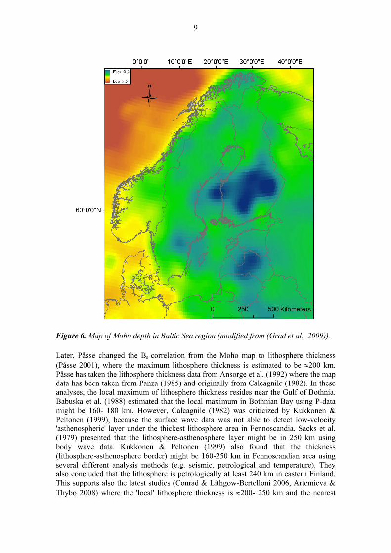
Figure 5. Map of ice recession in Fennoscandia (modified from Geological Survey of Sweden (2011)). In Påsse (1996) the uplift mechanism is modeled using three different parameter combinations (A1, B1, T1), (A2, B2, T2) and (A3, B3, T3). Påsse states (Påsse 1996) that “Resemblances exist between this (Moho) map and the map showing the variations in the values of the declining factor B1”. The parameter values B1-B3 are presented as computation results and there is no effort to connect them to Moho depth. In Påsse (1997) the fast and slow uplift mechanisms are presented. The correlation between the parameter Bs and Mohorovičić discontinuity map can be written as Eq. 2-6 where ct is the crustal thickness of the earth. Påsse used the Moho map from Kinck et al. (1993) which is quite similar to the latest more detailed Moho map (Grad et al. 2009) (Figure 6).
cts eB 067.0302 (2-6)
9
Figure 6. Map of Moho depth in Baltic Sea region (modified from (Grad et al. 2009)). Later, Påsse changed the Bs correlation from the Moho map to lithosphere thickness (Påsse 2001), where the maximum lithosphere thickness is estimated to be 200 km. Påsse has taken the lithosphere thickness data from Ansorge et al. (1992) where the map data has been taken from Panza (1985) and originally from Calcagnile (1982). In these analyses, the local maximum of lithosphere thickness resides near the Gulf of Bothnia. Babuska et al. (1988) estimated that the local maximum in Bothnian Bay using P-data might be 160- 180 km. However, Calcagnile (1982) was criticized by Kukkonen & Peltonen (1999), because the surface wave data was not able to detect low-velocity 'asthenospheric' layer under the thickest lithosphere area in Fennoscandia. Sacks et al. (1979) presented that the lithosphere-asthenosphere layer might be in 250 km using body wave data. Kukkonen & Peltonen (1999) also found that the thickness (lithosphere-asthenosphere border) might be 160-250 km in Fennoscandian area using several different analysis methods (e.g. seismic, petrological and temperature). They also concluded that the lithosphere is petrologically at least 240 km in eastern Finland. This supports also the latest studies (Conrad & Lithgow-Bertelloni 2006, Artemieva & Thybo 2008) where the 'local' lithosphere thickness is 200- 250 km and the nearest
10
local maximum is near Moscow, Russia. From this point of view the lithosphere thickness, a variable of Bs parameter, does not explain properly the inertia properties of Eq. 2-3, if the latest data is used. Due to the dissenting opinions about the lithosphere thickness, the estimation of the inertia factor Bs was decided to be based on a Moho map of Europe by Grad et al. (2009) (Figure 6). The Moho map describes the depth of the boundary between the Earth’s crust and the mantle (Mohorovičić discontinuity). Based on this fact, the Moho depth can be regarded as the crustal thickness of the Earth and the inertia factor Bs can be calculated using the Eq. 2-6.
2.3 Other research on land uplift in Fennoscandian area In addition to Påsse’s work there has been ongoing research on land uplift in Fennoscandian area by the means of geophysical modelling (viscoelastic models) and geodetic observation of present uplift values. Peltier has developed several glacial isostatic adjustment models. Global glacial history starting from the last glacial maximum to the present is modeled by the ice models ICE-3G (Tuskingham & Peltier 1991), ICE-4G (Peltier 1994) and ICE-5G (Peltier 2004). These models are closely related to viscoelastic models, where the iterative solution is a balance between the viscoelastic model, the relative sea level history and the estimated ice sheet thickness as a function of time (Peltier 1974, 1976 and 1996). Kurt Lambeck has also done extensive research on earth models and postglacial uplift (Lambeck et al. 1998a, 1998b; Lambeck & Purcell 2003). A Fortran implementation of the viscoelastic model has been presented by Spada & Stocchi (2007). All these models are based on earth structures and their physical responses to different types of stresses and deformations. These kinds of iterative multilayer solutions are computationally very demanding. Geodetic observation of present uplift values is another basis for land uplift modelling. The spatial (x, y, z) data is obtained by precise levellings (Mäkinen & Saaranen 1998) or precise GPS measurements, and the local land uplift is derived from measurement time series (Milne et al. 2001, Vestøl 2006, Lidberg et al. 2010). Another interesting model is based on the GRACE satellite data. This model uses observed earth gravity field and its changes as inputs. The gravitational uplift signal can be detected using absolute and relative gravimetry (Steffen et al. 2008, Steffen et al. 2009). In (Steffen et al. 2008) the GRACE satellite data was compared to the geophysical models with promising results. In precise measurement studies, data and predictions are based on short time scale observations (from several years to a couple of decades). Although the uplift rate can be estimated quite accurately from these observations, the time scale is too short to evaluate changes in the uplift rate or to fit a hyperbolic function with good reliability. Therefore, precise measurement extrapolation cannot be extended over thousands of years time span. This information can, however, be used for adjusting a hyperbolic function model. The uplift velocity can be taken directly to force the hyperbolic curves to follow the height difference over the years for which the precise uplift velocity is

11
computed. This has been done in Vuorela’s parametric model (Vuorela et al. 2009), for example. All these models (Påsse’s model based on hyperbolic tangents, viscoelastic models based on Earth’s geophysical qualities and uplift models based on precise measurements) serve different types of purposes. Geophysical models can be considered as ‘true’ earth models. When considering the isostatic rebound process at a certain location, these models take into account the dynamic effects of other regions globally. Thus the approach is quite different when compared to Påsse’s hyperbolic tangent function model. The hyperbolic tangent models are used for fitting mathematical curves to local observations using low complexity computations. There has been a debate whether or not hyperbolic functions are able to model the glacial isostatic adjustment sufficiently in Fennoscandia (Lambeck 2006). In his article Lambeck states that hyperbolic functions may lead to false conclusions or predictions due to insufficient shore level observation data. This is because of the lack of earth structure physics in Påsse’s hyperbolic function model (Lambeck 2006). According to (Lambeck 2006): “Hyperbolic functions are combinations of exponential functions, and for linear materials the stress relaxation can usually be defined as an exponential decay. Thus, it is not surprising that combinations of such functions can approximate rebound phenomenon. But describing the observation and understanding the underlying processes are two different things and the hyperbolic function description will not shed much light on the other.” It is true, that Påsse’s model as such does not rely on the geophysical properties of the structure of the Earth. Thus, fitting mathematical functions to collected data sets yields ambiguous results for the parameter values of these functions and the parameters cannot be interpreted as carrying any physical meaning. However, Påsse’s model utilizes only a few hyperbolic functions that are optimized for the Fennoscandia region, and this hyperbolic combination can be used with caution in this area for data fitting and extrapolation. In this study, the data sets overlap each other and they do not contain significant gaps so it is possible to evaluate and assess Påsse’s model with good accuracy.

12
3 INPUT DATA Two kind of input data were available in the land uplift model: one collected from lake basins, indicating the age of the sediment level where the environment changes from brackish water to fresh water, and the other collected from archaeological sites of prehistoric human activity, indicating the time when the particular location definitely represented dry land. Observations from the precise levellings or from GPS measurements were not used since they cover, at the best, only some decades.
3.1 Lake basin data This data set consists of 133 points that were taken from Vuorela et al. (2009). 94 of the points are from Finland and 39 points are from Sweden. The majority of the Finnish data points are originally from Eronen et al. (1995), where the isolation time of several lake basins in Finland due to the land uplift was studied. The isolation time from the Baltic Sea was based on drilled core samples taken from the bottom of the basins. The layer where the freshwater algae have replaced the saltwater algae was radiocarbon-dated. Also the estimate of the water level was determined based on observations from the surrounding landscape. The Finnish data points were selected so that only lakes and mires that had clear outlets were included and in cases where there were two radiocarbon dated samples from the same place the older sample was taken. A list of these data points (modified from Vuorela et al. 2009) is in appendix 3. The location of the points is shown in Figure 6 (blue points).
3.2 Archaeological data This data set consists of 258 data points that were taken from Tallavaara et al. (2010). The data sets includes house and village sites, graves, ancient fireplaces etc.; for further description, see also Pesonen et al. (2011). The archaelogical data points represent the upper limit for the water level. The location of the points is shown in Figure 6 (red points). This data set was added with four points from the register of The National Board of Antiquities (Museovirasto 2011). The data from The National Board of Antiquities was used only in the Satakunta area, closest to the Olkiluoto site, due to the laborious data search and handling.

13
Figure 7. The lake basin dating locations (blue points) and the archaeological site data set locations (red points) in Finland and Sweden.

14
4 REFINEMENT OF PÅSSE’S UPLIFT MODEL Both data sets involved the usage of 14C radiocarbon dating procedure. The “OxCal” software by Oxford Radiocarbon Accelerator Unit (2010) was used to convert the 14C radiocarbon dating results into calendar year taking into account the underlying uncertainties. In Figure 8, an example of the calibration and conversion procedure of the data point from Lake Vähäjärvi in Eura is presented. Obviously, the dating procedure yields quite a complex-shaped error distribution for the age of each data point. Another source of uncertainty is the elevation value of the data points. This uncertainty was taken into account by applying Gaussian distribution (standard deviation of 3 m was considered to be a sufficient measure for uncertainty in terms of e.g. erosion connected with lake tilting) to each elevation datum in the data sets. Monte Carlo simulation involving 1000 realizations was then used to obtain the probabilistic estimates of the As and Bs parameter values of Påsse’s shore line displacement model. The estimation of model parameters proceeded as follows (the flow chart in Figure 9). The first task was to find the neighbouring points for the data point and calculate the As and Bs parameters. The 10 nearest points were selected including the point in question and at least 3 points from the lake basin data set.
Figure 8. Screen capture from the OxCal program. The 14C age (6960) and the uncertainty (170) are the inputs. The line indicates the calibration curve while the error distribution of the calendar age (95.4 % confidence) is shown in dark grey.

15
Check {As Bs}, if data points stay above sea level
Neighborhood of data points
(max. 10 points; at least 3 lake basin data set
points)
Prehistoric population data
points
Lake basin data points
Initial {As Ts Bs} (from figs. 4,5 &
6)
{As Bs} optimization procedure
Derivative based As
estimation
Current land uplift rate
{As Bs}value pair
{As Bs}value pair
Bs
Ts
Figure 9. The flow chart of the estimation process. As a starting point, a {As Bs} parameter value pair was selected from the model and data of Påsse (2001) and Grad et al. (2009), presented in Figures 4 and 6. The value of Ts parameter was taken from Geological Survey of Sweden (2011), presented in Figure 5. The optimization process for estimating As and Bs parameters was carried out using an orthogonal least squares optimization method. A region in the {As Bs} parameter space was defined where the true parameter values were supposed to lie according to the data. This region was assigned to a cost function: the less probable the obtained parameter values were, the higher was the cost. The minimum value of the cost function was dependent on the initial parameter values of Figures 4 and 6 for the particular site, i.e. it is assumed that (Påsse 2001) is at least approximately right in the larger scale. An optimization procedure was then initiated and performed to produce all the parameter value pairs corresponding to the minimum values of cost functions. The curve fitting was done in the MatLab computation environment using the fminsearch-function, which is based on the Nelder-Mead method presented in Nelder & Mead (1965). As the prehistoric population data set presents archaeological evidence on human residence, the corresponding sites should locate above the sea level at the particular time. If the parameter values {As Bs} from the previous step indicated the opposite, the parameter values were changed step-by-step until the resulting land uplift curve remained below the elevation obtained from the selected neighbouring data points. Thus, an adjusted parameter value pair was obtained as the result. If no correction was needed, i.e. the elevation of the prehistoric population data was higher than the sea level at the particular time, this data set was ignored. As a comparison, another method, based on the present land uplift rate (Figure 1) and the modelling function, was used in the parameter estimation. The applied method is illustrated in the report by Vuorela et al. (2009). The Bs parameter was fixed to the value obtained by using the method described above and the As value satisfying the current land uplift rate (Poutanen 2011) was selected to give another parameter value pair.

16
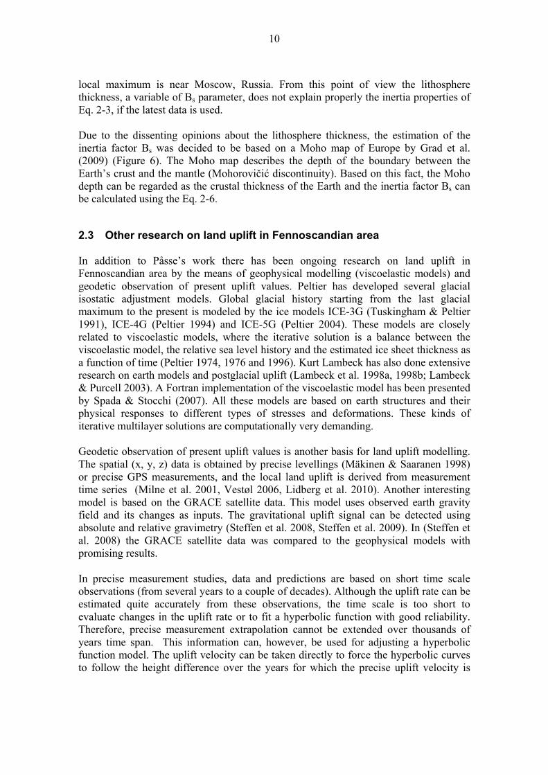
The statistical estimation of parameters was performed using a Monte Carlo method (Mosegaard & Sambridge 2002). In this way, the resulting parameters were actually represented by probability distributions. The probability distributions were smoothed with kernel density estimation in order to get more reliable estimates for the parameter values. The calculation space was defined for each data point so that the particular data point occurred in the centre of the space. Thus, the resulting probabilistic parameter value pair was assigned to the location of the data point around which the space was located. During the estimation process it became clear that the download factor As, the ice recession parameter Ts and the inertia factor Bs have a strong relationship in Eq. 2-3. This can be seen from the error surface in Figure 10. The error surface is shaped like a diagonal canyon without a single minimum. In the case of Figure 10, the parameter Ts can be chosen and the other parameter As (or vice versa) can be found using the nearest minimum from the surface. Based on the error surface the relationship between the slow uplift parameters seems to be almost linear. Certain expected values can be used for 'guiding' the error surface and thus for the estimation of optimal parameters. For instance, ice is recessed over a certain point at a certain time (with error margins), so this parameter cannot be arbitrary. Using the expected values the error surface can be presented in a form of Figure 11.
Figure 10. An error surface describing the behavior of the parameters As, Ts and Bs.
17
Figure 11. An error surface created using the aid of expected values.
18
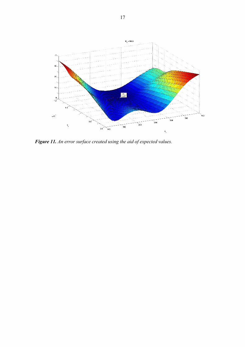
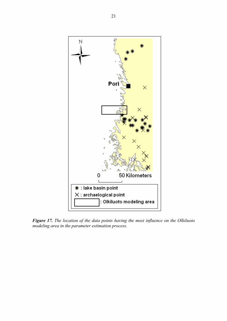
5 RESULTS The estimation procedure was carried out using both eustatic models presented in Figure 3. The results include therefore two different values for As and Bs parameter calculated as described in chapter 4. The distributions of 1000 realizations of the As parameters obtained from Monte Carlo simulation are presented in Figure 12. The initial As, Ts and Bs values for Rapajärvi in Rauma (lat: 61° 5.409', lon: 21° 42.453', coordinate system: WGS 84) were 266, 10929 and 7318, respectively, according to Figures 4, 5 and 6. Figure 13 presents the interpolated raster images of the As parameters obtained as the most probable values. In Figure 14, the images of the Bs parameters are presented using both eustatic models. The results of the As parameter calculated using a derivative-based process (Vuorela et al., 2009) are presented in Figure 15. The results from Olkiluoto modeling area are in Figure 16. These As surfaces correspond to the area of the digital elevation model presented in Pohjola et al. (2009). The whole area of Olkiluoto Island and surroundings is 20*48 km2 in size that covers Olkiluoto Island and the area surrounding it. The surfaces were interpolated using a thin plate spline interpolation (Donaldo & Belongo 2002). In Figure 17 the data points having the most influence on the Olkiluoto modelling area are presented.
Figure 12. The simulation results of the As parameter for Rapajärvi in Rauma.
160 180 200 220 2400
0.01
0.02
0.03
0.04
0.05
0.06
0.07
Mean: 198.06 m
Median: 197.45 m
A s distribution (Påsse-eustatic model)
160 180 200 220 2400
0.01
0.02
0.03
0.04
0.05
0.06
0.07
Mean: 196.73 m
Median: 196.89 m
As distribution (Punning-eustatic model)

19
Figure 13. Maps of As parameters in the area of Finland. The left-hand side map is calculated using Påsse’s eustatic model and the right-hand side map using Punning et al.’s. eustatic model.
Figure 14. Maps of Bs parameters in the area of Finland. The left-hand side map is calculated using Påsse’s eustatic model and the right-hand side map using Punning et al.’s. eustatic model.

20
Figure 15. Maps of estimated As parameters using a derivative-based process described in Vuorela et al. (2009). The left-hand side map is calculated using Påsse’s eustatic model and the right-hand side map using Punning et al.’s eustatic model.
Figure 16. As surfaces of the Olkiluoto area created using Påsse’s (top figure) and Punning et al.’s. (bottom figure) eustatic models.
21
Figure 17. The location of the data points having the most influence on the Olkiluoto modeling area in the parameter estimation process.

22
6 DISCUSSION AND CONCLUSIONS The aim of the presented study was to refine the parameters of Påsse’s land uplift model taking into account previously unavailable data and an alternative model of eustatic sea level rise. Our particular interest was to find out if variations from the rather symmetric form of the earlier models of the land uplift can be detected based on the available data and modeling methods. When comparing our results for the As parameter value (Figure 13) to those presented in Figure 4, it can be seen that the area of the largest As values has been shifted to Central Finland. This behaviour can be related to the maps of the Bs parameter presented in Figure 14. It seems that the Bs parameter has a major influence on the estimation of the As parameter value. The maps of the Bs parameters presented in Figure 14 coincide well with the Moho map in Figure 6. Generally the results for As and Bs parameters do not differ significantly when using either Påsse’s or Punning et al.’s eustatic model. Another reference to our results is that proposed in Vuorela et al. (2009). In this report, the parameters of land uplift model have been estimated using a difference-based method and current land uplift rates. The interpolated raster images of As parameters from the difference-based method are presented in Figure 15. The method images coincide well with Figure 4 but the As parameter values are significantly larger. When looking at the raster image of As parameter in Figure 13, sharp changes in the parameter values can be noticed throughout Finland. Most likely these kinds of anomalies are caused by uncertainties and inaccuracies in the data but some differences in the land uplift rate can also be revealed after statistical examination. A comparison for the possible differences is found in Poutanen (2011), where the observed land uplift rate based on three precise levellings in Finland has been presented. From the observed land uplift rate can be noticed that there may exist some local variations in land uplift in Finland. Further investigation involving additional data is needed here. From Figure 16, in the modeling area at Olkiluoto, it can be noticed that both As parameter maps using Påsse’s and Punning et al.’s eustatic models, coincide generally well but there are also slight differences in the values and shapes of the maps. As a conclusion, the proposed procedure for the estimation of the parameters of Påsse’s land uplift model gives more detailed information about the variation of the uplift process. Other advantages of this approach are the usage of more accurate eustatic model as well as incorporating source data not previously employed.

23
REFERENCES Alhonen, P., 1967. Palaeolimnological investigations of three inland lakes in south-western Finland. Acta Botanica Fennica 76, 59 pp. Alhonen, P., 1981. Stratigraphical studies on Lake Iidesjärvi sediments. Part I: Environmental changes and palaeolimnological development. Bulletin of Geological Society of Finland 53 (2), 97-107. Alhonen, P., Eronen, M., Nunez, M., Salomaa, R. & Uusinoka, R., 1978. A contribution to Holocene shore displacement and environmental development in Vantaa, South Finland: the stratigraphy of Lake Lammaslampi. Bulletin of Geological Society of Finland 50, 69-79. Ansorge, J., Blundell, D. & Mueller, S., 1992. Europe’s lithosphere – seismic structure. In A continent revealed. The European Geotraverse. Ed. D. Blundell, R. Freeman & S. Mueller, 33–69. Artemieva, I.M. & Thybo, H., 2008. Deep Norden: Highlights of the lithospheric structure of Northern Europe, Iceland, and Greenland. Episodes 31 (1), 98-106. Babuška, V., Plomerová, J. & Pajdušák, P., 1988. Seismologically determined deep lithosphere structure in Fennoscandia. Geol. Fören. Stockholm Förh. 110, 380–382. Bard, E., Hamelin, B., Arnold, M., Montaggioni, L., Cabioch, G., Faure, G. & Rougerie, F., 1996. Deglacial sea-level record from Tahiti corals and the timing of global meltwater discharge, Nature 382, 241–244. Berglund, M., 2005. The Holocene shore displacement of Gästrikland, eastern Sweden: a contribution to the knowledge of Scandinavian glacio-isostatic uplift. Journal of Quaternary Science 20 (6), 519-531. Brydsten, L., Engqvist, A.., Näslund, J.-O. & Lindborg, T., 2009. Expected extreme sea levels at Forsmark and Laxemar–Simpevarp up until year 2100, Swedish Nuclear Fuel and Waste Management Co. Technical Report TR-09-21. Stockholm. ISSN 1404-0344. Calcagnile, G., 1982. The lithosphere-astenosphere system in Fennoscandia. Tectonophysics 90, 19-35. Cathles, L.M., 1975. The viscosity of the earth’s mantle. Princeton University Press. Princeton. Chappell, J. & Polach, H., 1991. Post-glacial sea-level rise from a coral record at Huon Peninsula, Papua New Guinea. Nature 349, 147–149. Clark, R.D., Farrell, W.E. & Peltier, W.R., 1978. Global changes in postglacial sea level: a numerical calculation. Quaternary Research 9, 265–287.

24
Conrad, C.P. & Lithgow-Bertelloni, C., 2006. Influence of continental roots and asthenosphere on plate-mantle coupling. Geophysical Research Letters 33. Donaldo, G. & Belonge, S., 2002. Approximate Thin Plate Spline Mappings. In A. Heyden, G. Sparr, M. Nielsen & P. Johansen (eds.): Lecture Notes in Computer Science, Vol. 2352, 21-31, Springer Berlin Heidelberg. Eronen, M., 1974. The history of the Litorina Sea and associated Holocene events. Soc. Sci. Fennica, Comm. Phys.-Meth. 44 (4), 79-195. Eronen, M., Heikkinen, O. & Tikkanen, M., 1982. Holocene development and present hydrology of Lake Pyhäjärvi in Satakunta, southwestern Finland. Fennia 160 (2), 195-223. Eronen, M., Glückert, G., van de Plassche, O., van der Plicht, J. & Rantala, P., 1995. Land Uplift In The Olkiluoto-Pyhäjärvi Area, Southwestern Finland During The Last 8000 Years. Nuclear Waste Commission of Finnish Power Plants. YTJ-95-17. Eronen, M., Glückert, G., van der Plassche, O., van der Plicht, J., Rajala, P. & Rantala, P., 1995a. The postglacial radiocarbon dated shoreline data of the Baltic in Finland for the Nordic data of land uplift and shorelines. A NKS/KAN 3 project report, Stockholm (in press). Eronen, M., Glückert, G., Hatakka, L., van de Plassche, O., van der Plicht, J. & Rantala, P., 2001. Rates of Holocene isostatic uplift and relative sea-level lowering of the Baltic in SW Finland based on studies of isolation contacts. Boreas 30 (1), 17-30. Fairbanks, R.G., 1989. A 17,000-year glacio-eustatic sea level record: influence of glacial melting rates on the Younger Dryas event and deep-ocean circulation, Nature 342, 637-642. Geological Survey of Sweden., 2011. Kartgenerator. [WWW]. [referred at 21.9.2011]. Web address: http://maps2.sgu.se/kartgenerator/sv/maporder.html. Glückert, G., 1978. Das Deltakomplex von Kiikalannummi am 3. Salpausselkä in Südwestfinnland. Publ. Dept. Quarternary Geol., Univ. Turku, 35, 26 pp. Glückert, G., 1979. Shore-level displacement of the Baltic and the history of vegetation in the Salpausselkä belt, western Uusimaa, South Finland. Publ. Dept. Quarternary Geol., Univ. Turku, 39, 77 p. Glückert, G., Illmer, K., Kankainen, T., Rantala, P. & Räsänen, M., 1992. Vegetational history in the surroundings of Lake Littoinen and its natural dystrofication. Publ. Dept. Quarternary Geol., Univ. Turku, 75, 27 pp. Glückert, G., Peltola, H. & Rantala, P., 1998. Landhöjning och Östersjöns strandförskjutning i Kronoby-Larsmo-området, mellersta Österbotten, under de senaste 3000 åren. Turun yliopiston maaperägeologian osaston julkaisuja 81. Turku: Turun yliopisto, 15 p.

25
Grad, M., Tiira, T., & ESC Working Group., 2009. The Moho depth map of the European Plate, Geophys. J. Int 176, 279–292. Hedenström, A. 2001., Early Holocene shore displacement in eastern Svealand, Sweden, based on diatom stratigraphy, radiocarbon chronology and geochemical parameters. Quaternaria. Ser. A: Theses and Research Papers No. 10. Stockholm University, 48 p. Hedenström, A. & Risberg, J., 2003. Shore displacement in northern Uppland during the last 6500 calender years. SKB technical report, TR-03-17. Hyvärinen, H. 1966., Studies on the late-Quarternary history of Pielis-Karelia, eastern Finland. Soc. Scient. Fennica. Comment Biol. 29 (4), 72 pp. Hyvärinen, H. 1979., Bakunkärrsträsket: a stratigraphical site relevant to the Litorina shore discplacement near Helsinki. Terra 91 (1), 15-20. Hyvärinen, H., 1980. Relative sea-level changes near Helsinki, southern Finland, during early Litorina times. Bulletin of Geological Society of Finland 52 (2), 207-219. Hyvärinen, H., 1984. The Mastogloia stage in the Baltic Sea history: Diatom evidence from southern Finland. Bulletin of Geological Society of Finland 56 (1-2), 99-115. Ikonen, A.T.K. & Lipping, T., 2011. Proceedings of a Seminar on Sea Level Displacement and Bedrock Uplift, 10-11 June 2010, Pori, Finland, Working Report 2011-07. Posiva Oy, Eurajoki, Finland. Jungner, H. & Sonninen, E., 1983. Radiocarbon dates II. Radiocarbon dating laboratory, University of Helsinki. Report no. 2, 1-121. Kinck, J.J., Husebye, E.S. & Larsson, F.R., 1993. The Moho depth distribution in Fennoscandia and the regional tectonic evolution from Archean to Permian times. Precambrian Research 64, 23-51. Kukkonen, I.T. & Peltonen, P., 1999. Xenolith-controlled geotherm for the central Fennoscandian Shield: implications for lithosphere-asthenosphere relations. Tectonophysics 304, 301-315. Lambeck K., 2006, Hyperbolic tangents are no substitute for simple classical physics, GFF 128, 349-350. Lambeck, K., Smither, C. and Johnston, P., 1998a. Sea-level change, glacial rebound and mantle viscosity for northern Europe. Geophys. J. Int. 134, 102-144. Lambeck, K., Smither, C. and Ekman, M., 1998b. Tests of glacial rebound models for Fennoscandinavia based on instrumented sea- and lake-level records. Geophys. J. Int., 135 375-387.

26
Lambeck, K. & Purcell, A., 2003. Glacial Rebound and Crustal Stress in Finland, Working Report 2003-10. Posiva Oy, Eurajoki, Finland. Lehmuskoski, P. 2010., Precise Levelling Campaigns at Olkiluoto in 2008 and 2009. Working Report 2010-30. Posiva Oy, Eurajoki, Finland. Lehto, K. 2001., Installation of Groundwater Observation Tubes at Olkiluoto in Eurajoki 2001, Working Report 2001-39. Posiva Oy, Eurajoki, Finland. Lidberg, M., Johansson, J. M., Schernecka, H-G., Milne, G. A., 2010, Recent results based on continuous GPS observations of the GIA process in Fennoscandia from BIFROST, Journal of Geodynamics 50 (1), 8-18. Lindborg, T. & Rubio Lind, L., 2006. Long-term development of the super-regional area of Olkiluoto/Forsmark/Laxemar. Minutes from the Posiva and SKB workshop, October 12-13, 2006 Rånäs Slott, Sweden, Swedish Nuclear Fuel and Waste Management Co. Report P 06-302, 2006. Stockholm. ISSN 1651-4416. Madsen, K.S., Høyer, J.L. & Tscherning, C.C., 2007. Near-coastal satellite altimetry: Sea surface height variability in the North Sea-Baltic Sea area. Geophysical Research Letters 34. Meehl, G.A., Stocker, T.F., Collins, W.D., Friedlingstein, P., Gaye, A.T., Gregory, J.M., Kitoh, A., Knutti, R., Murphy, J.M., Noda, A., Raper, S.C.B., Watterson, I.G., Weaver, A.J. & Zhao, Z.-C., 2007. Global Climate Projections. In S. Solomon, D. Qin, M. Manning, Z. Chen, M. Marquis, K.B. Averyt, M. Tignor & H.L. Miller (eds.): Climate Change 2007: The Physical Science Basis. Contribution of Working Group I to the Forth Assessment Report of the Intergovernmental Panel on Climate Change, 747-845, Cambridge University Press. Miettinen, A., 2002. Relative sea level changes in the eastern part of the Gulf of Finland during the last 8000 years. Annales Academiae Scientiarum Fennicae, Geologica-Geographica 162, 100 pp. (Ph.D. Thesis). Miettinen, A., Eronen, M. & Hyvärinen, H., 1999. Land uplift and relative sea-level changes in the Loviisa area, southeastern Finland, during the last 8000 years. Posiva Report 99-28, Posiva Oy, Eurajoki, Finland. Miettinen, A., Jansson, H., Alenius, T. & Haggrén, G., 2007. Late Holocene sea-level changes along the southern coast of Finland, Baltic Sea. In: Quaternary land-ocean interactions: sea-level change, sediments and tsunami. Marine Geology 242 (1-3), 27-38. Milne, G. A., Davis, J. L., Mitrovica, J. X., Scherneck, H.-G., Johansson J. M., Vermeer, M., Koivula, H., 2001, Space-Geodetic Constraints on Glacial Isostatic Adjustment in Fennoscandia, Science 291, 2381-2385. Mosegaard, K. & Sambridge, M., 2002. Monte Carlo analysis of inversion problems. Inverse Problems 18, R29-R54.

27
Museovirasto, 2011. Rekisteriportaali. [WWW]. [referred at 3.1.2011]. Web address: http://kulttuuriymparisto.nba.fi/netsovellus/rekisteriportaali/portti/default.aspx. Mäkinen, J. & Saaranen, V., 1998. Determination of post-glacial land uplift from the three precise levellings in Finland. Journal of Geodesy 72, 516-529. Nelder, J. & Mead, R., 1965. A simplex method for function minimization, Computer Journal 7, 308–313. Oxford Radiocarbon Accelerator Unit. 2010. OxCal. [Online] (Updated 5 Apr 2010) Available at: http://c14.arch.ox.ac.uk/embed.php?File =oxcal.html. Panza, G. F., 1985. Lateral variations in the lithosphere in correspondence of the Southern Segment of EGT. In: D. A. Galson and St. Mueller (eds), Second EGT Workshop: The Southern Segment, 47-51, European Science Foundation, Strasbourg, France. Peltier, W.R., 1974. The impulse response of a Maxwell Earth. Reviews of Geophysics and Space Physics 12 (4), 649–669. Peltier, W.R., 1976. Glacial-isostatic adjustment—II. The inverse problem. Geophysical Journal of the Royal Astronomical Society 46, 669–705. Peltier, W. R., 1994. Ice Age Paleotopography. Science 265, 195–201. Peltier W. R, 1996. Mantle Viscosity and Ice-Age Ice Sheet Topography, Science 273, 1359-1364. Peltier W.R, 2004. Global Glacial Isostasy and the Surface of the Ice-Age Earth: The ICE-5G (VM2) Model and GRACE, Invited Paper, Annual Review of Earth and Planetary Science 32, 111-149. Pesonen, P., Kammonen, J., Moltchanova, E., Oinonen, M. & Onkamo, P., 2011., Archaelogical radiocarbon dates and ancient shorelines – resources and reservoirs. Proceedings of a Seminar on Sea Level Displacement and Bedrock Uplift, 10-11 June 2010, Pori, Finland, Working Report 2011-07. Posiva Oy, Eurajoki, Finland. pp. 119-129. Pohjola, J., Turunen, J. & Lipping, T., 2009. Creating high-resolution digital elevation model using thin plate spline interpolation and Monte Carlo simulation. Working Report 2009-56. Posiva Oy, Eurajoki, Finland. Poutanen, M., 2011. Present bedrock movements and land uplift. Proceedings of a Seminar on Sea Level Displacement and Bedrock Uplift, 10-11 June 2010, Pori, Finland, Working Report 2011-07. Posiva Oy, Eurajoki, Finland. pp. 25-35. Punning, Y.M., 1987. Holocene eustatic oscillations of the Baltic Sea level. Journal of Coastal research 3 (4), 505-513. Charlottesville, ISSN 0749-0208.
28
Påsse, T., 1996. A mathematical model of the shore level displacement in Fennoscandia, Swedish Nuclear Fuel and Waste Management Co. Technical Report TR-96-24, 1996. Stockholm. Påsse, T., 1997. A mathematical model of past, present and future shore level displacement in Fennoscandia, Swedish Nuclear Fuel and Waste Management Co. Technical Report TR-97-28, 1997. Stockholm. ISSN 0284-3757. Påsse, T., 2001. An empirical model of glacio-isostatic movements and shore level displacement in Fennoscandia, Swedish Nuclear Fuel and Waste Management Co. Report R-01-41, 2001. Stockholm. ISSN 1402-3091. Påsse, T., 2006. Never forget the highest coastline! – Reply to “Hyperbolic tangents are not substitute for simple classical physics”, GFF 128, 350-351. Påsse, T. & Daniels, J., 2011. Comparison between a new and an old semi-empirical Fennoscandian shore-level model. Proceedings of a Seminar on Sea Level Displacement and Bedrock Uplift, 10-11 June 2010, Pori, Finland, Working Report 2011-07. Posiva Oy, Eurajoki, Finland. pp. 47-50. Ristaniemi, O., 1984. Shoreline displacement of the Baltic during the Ancylus stage in the Karjalohja-Kisko area, the Salpausselkä belt, SW-Finland. Publ. Dept. Quarternary Geol., Univ. Turku, 53, 75 pp. Ristaniemi, O., 1987. The highest shore and Ancylus limit of the Baltic Sea and the ancient Lake Päijänne in central Finland. Ann. Univ. Turkuensis, Ser. C, 59, 102 pp. Ristaniemi, O. & Glückert, G., 1988. Ancylus- ja Litorinatransgressiot Lounais-Suomessa. In: Lappalainen, V. & Papunen, H. (eds.): Tutkimuksia geologian alalta. Ann. Univ. Turkuensis, Ser. C, 67, pp. 129-145. Saarnisto, M., 1979. Deglaciation north of the Gulf of Bothnia. Abstact: Deglaciation yngre än 10000 BP, Uppsalasymposiet 1979, 1 p. Saarnisto, M., 1981. Holocene emergence history and stratigraphy in the area north of the Gulf of Bothnia. Ann. Acad. Sci. Fennicae, Ser. A III, 130, 42 pp. Sacks, I.S., Snoke, J.A. & Husebye, E.S., 1979. Lithosphere thickness beneath the Baltic Shield. Tectonophysics 56, 101-110. Salomaa, R., 1982. Post-glacial shoreline displacement in the Lauhanvuori area, western Finland. Ann. Acad. Sci. Fennicae, Ser. I, III, 134, 81-97. Salomaa, R., & Matiskainen, H., 1983. Rannansiirtyminen ja arkeologinen kronologia Etelä-Pohjanmaalla. Arkeologian päivät 7-8.4.1983 Lammin biolog. tutkimusasemalla. Karhunhammas, 7, 21-36.

29
Seppä, H. & Tikkanen, M., 1998. The isolation of Kruunuvuorenlampi, southern Finland, and implications for Holocene shore displacement models of the Finnish south coast. Journal of Paleolimnology 19 (4), 385-398. Seppä, H., Tikkanen, M. & Shemeikka, P., 2000. Late-Holocene shore displacement of the Finnish south coast: diatom, litho- and chemostratigraphic evidence from three isolation basins. Boreas 29 (3), 219-231. Spada G., Stocchi P., 2007. SELEN: A Fortran 90 program for solving the “sea-level equation”, Computers & Geosciences 33, 538–562. Steffen H., Denker H., Müller J., 2008. Glacial isostatic adjustment in Fennoscandia from GRACE data and comparison with geodynamical models. Journal of Geodynamics 46, 155-164. Steffen H., Gitlein O., Denker H., Müller J., Timmen L., 2009, Present rate of uplift in Fennoscandia from GRACE and absolute gravimetry, Tectonophysics 474, 69–77. Tallavaara, M., Pesonen, P. & Oinonen, M., 2010. Prehistoric population history in eastern Fennoscandia, Journal of Archaeological Science 37, 251–260. Tikkanen, M. & Oksanen, J., 2002. Late Weichselian and Holoscene shore displacement history of the Baltic Sea in Finland, Fennia 180, 9–20. ISSN 0015-0010. Tolonen, M., 1987. Vegetational history in coastal SW Finland studied on a lake and a peat bog by pollen charcoal analyses. Annales Botanici Fennici 24, 353-370. Tolonen, K. & Tolonen, M., 1988. Synchronous pollen changes and traditional land use in south Finland, studied from three adjecent sites. A lake, a bog and a forest soil. In: Lang, G. & Schlüchter, C. (eds.): Lake and River Environments During the last 15000 years, pp. 83-97, Balkema, Rotterdam. Toropainen, V., 2009. Installation of Groundwater Observation Tubes OL-PVP30–35 at Olkiluoto in Eurajoki 2009, Working Report 2009-27. Posiva Oy, Eurajoki, Finland. Tushingham, A.M. & Peltier, W.R., 1992. Validation of the ICE-3G Model of Wurm-Wisconsin Deglaciation Using a Global Data Base of Relative Sea Level Histories, J. Geophys. Res. 97, 3285-3304. Vestøl, O., 2006. Determination of postglacial land uplift in Fennoscandia from leveling, tide-gauges and continuous GPS stations using least squares collocation. Journal of Geodesy 80, 248-258. Vuorela, A., Penttinen, T. & Lahdenperä, A-M., 2009. Review of Bothnian Sea shore-level displacement data and use of a GIS tool to estimate isostatic uplift, Working Report 2009-17. Posiva Oy, Eurajoki, Finland.

30
APPENDIX 1: COMPARISON BETWEEN 2001 AND 2010 LAND UPLIFT MODELS BY TORE PÅSSE Tore Påsse has further developed his 2001 model (Påsse 2001) in order to reduce the number of parameters. In his newest model (Påsse 2010) the concept of fast and slow uplift has been changed to viscous and elastic uplift. The viscous uplift parameters can be derived from the elastic uplift parameters. The total number of free parameters can be reduced from 6 to 2 using the following scheme. Land uplift (U, in m) can be estimated using the 2010 model as:
vvv B
tT
B
TAU arctanarctan
2
eee B
tT
B
TA arctanarctan
2
(A1-1)
where Av is the download factor (m) for the viscous uplift (which can be interpreted as the fast uplift in the 2001 model), T (year) is the time for the maximal uplift rate, i.e. the symmetry point of the arctan function, t (year) is the variable time and Bv (year-1) is the relaxation factor for the viscous uplift (inertia factor in the 2001 model). In the calculations T and t are counted in calendar years. The variables Ae, and Be correspond in a similar way to the elastic (slow) uplift. As a result of the modelling, it is possible to reduce the variables in Eq. A1-1 to only two unknown variables, Ae (m) and T (year). The download factor for the viscous uplift Av (m) is derived from the download factor Ae for the elastic uplift:
6.49.1 ev AA (A1-2)
The relaxation factor for the viscous uplift Bv (year-1) is related to Av (m). Bv (year-1) is thus calculated from:
623367.7 vv AB (A1-3)
The relaxation factor for the elastic uplift Be is given a constant value of 600 (year-1). Påsse states in (Påsse 2010): “However, the history of the land uplift is somewhat more complex as the uplift was somewhat slower during the interval 13 500 – 11 500 BP. This irregularity has given a condition where the uplift is most easily modelled by two different uplift formulae, which means that uplift can be calculated by four unknown variables these are two down load-factors for the elastic uplift and two times for the maximal uplift rate. In this paper this variables are named A1 and A2 respectively T1 and T2.”
31
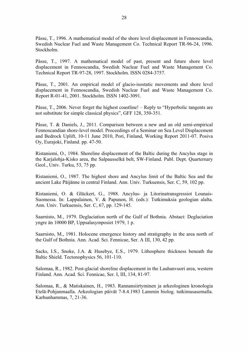
Unfortunately Påsse does not give any information on how these variables are combined for the final result. Also the indication of the slower uplift in time period 13500 - 11500 BP seems to contradict with the previous work, because in Påsse (2001), he shows that the time period in question was the time of the fast uplift as shown in Figure A1.1. On the other hand, the unclear statement of slower uplift may be the caused by the differences between the two models. In Olkiluoto and the surrounding study area, there are no dated points from the 13500 -11500 BP time period that would require the use of A1, A2, T1 and T2 parameters. The comparison between the 2001 and 2010 models was computed using the data set from the Lower Satakunta area presented in Figure 7. For the point in question, 9 nearest points were chosen to average the results. The lake sediment data is assumed to follow the lake isolation from the sea, but the archaeological data is the upper limit for the water level.
Figure A1.1. An example of the effects of the fast uplift in Sweden (Påsse 2001). In Figure A1.2, the 2001 and 2010 land uplift curves (using the maximum values from the histograms in Figure A1.3 and Påsse’s 2001 eustatic water level estimate) are shown.

32
Figure A1.2. Two different estimates of land uplift using the 2001 and 2010 models of Påsse.
Figure A1.3. Ae, Te, As and Ts estimates of land uplift.

33
Table A1.1. Parameters used in the example in Figure A1.2.
Method As [m] Ts [y] Ae [m] Te [y] 2001_lake 204 10476 2001_archaeo 255 10971 2010_lake 154 11473 2010_archaeo 100 10971
The land uplift curves were computed for both datasets separately. In the example presented in Figure A1.2, the parameters in Table A1.1 were used. Based on the Figure A1.2, it seems that the 2010 model is more sensitive to the parameter changes than the 2001 model. Also, Påsse does not explain the physical explanation for the elastic uplift parameter Ae, as in the 2001 model, where the As is said to represent half of the total depression of the crust in meters related to the load by the ice sheet. In Figure A1.4, three different Te parameters are presented in colours. Blue curves represent Te = 8500 years, Te = 10500 in red and Te =12500 in black. Ae parameters varies from 50, 70, 90, 110, 130, 150, 170 and 190 (bottom to top).
Figure A1.4. Påsse’s 2010 model with Ae and Te parameters (Ae estimates with increases of 20).
Te=8500 Te=10500 Te=12500
Ae=190
Ae=50

34
APPENDIX 2: UPDATED DIGITAL TERRAIN MODEL The original digital terrain model (DTM) has been presented in Pohjola et al. (2009). After this the DTM has been updated with new information and some artifacts have been corrected. The main source of new information has been Posiva Oy’s own sonar measurements in the summer and autumn of 2009. There has also been minor data point additions from other sources. In Figure A2.1, the locations of new data points are presented and the new data sources are described in Table A2.1. Specifically the area of Sorkanlahti Bay, where the depth of the sea was largely exaggerated due to lack of data, was corrected with the new data. The comparison between the updated and the previous DTM in the Sorkanlahti area is in Figure A2.2.
Figure A2.1. Source data points added to the version of (Pohjola et al. 2009). Table A2.1. Summary of the source data sets added to the version of (Pohjola et al. 2009).
Name of the data set
Year of acquisition Type of the data set
Precision
Sonar measurements by Posiva
2009 Sonar measure-ment lines
± 0.5 m (95 % confidence)
Prism measurements 2009 Elevation data points
± 0.01 m (95 % confidence)
Standpipe (SP) and core drilled borehole (CB) measurements
SP: 2001 (Lehto 2001), 2009 (Toropainen 2009). CB: 2007- 2009.
Elevation data points
± 0.01 m (95 % confidence)
Reedbed studies 2007-2008 Elevation data points
± 0.3 m (95 % confidence)

35
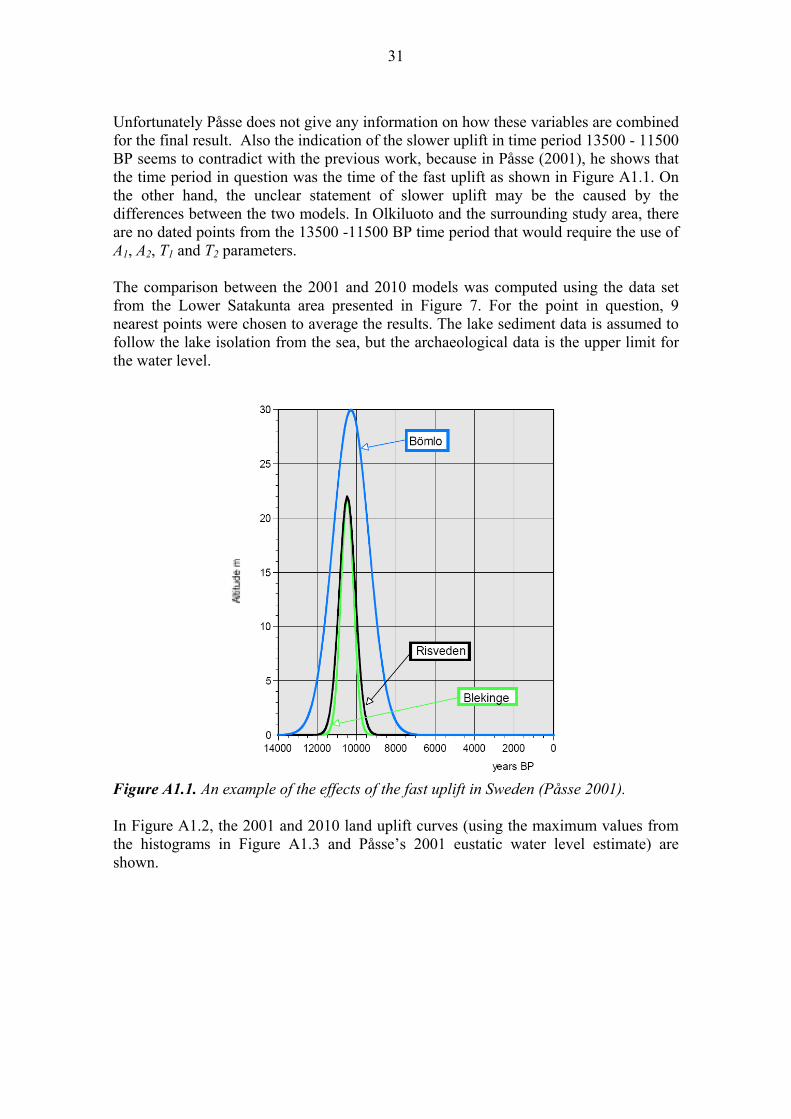
Figure A2.2. The Sorkanlahti area before (left column) and after (right column) the update of the terrain model. In addition two alternative models of the DTM were created. In the first one the terrain surface was smoothed with low-pass filtering. The size of the low-pass filter was 3*3 pixels. In the second alternative model the local maximums and minimums were emphasized. However, the value for the emphasized maximum or minimum stayed inside the confidence limits of the point in question. In Figure A2.3 the alternative DTMs and the difference surfaces between the original DTM and the alternative models in the Sorkanlahti area are presented.
36
Figure A2.3. The alternative models of the DTM and the difference surfaces between the original DTM and the two alternative models in the Sorkanlahti area.

37
AP
PE
ND
IX 3
: L
AK
E B
AS
IN D
AT
A P
OIN
TS
T
he li
st in
Tab
le A
3.1
desc
ribe
s th
e 13
3 da
ta p
oint
s in
the
lake
bas
in d
ata
set i
n ch
apte
r 3.
1.
Nam
e: th
e na
me
of th
e la
ke o
r m
ire
in q
uest
ion.
L
ocal
ity:
the
nam
e of
the
mun
icip
alit
y.
N:
latit
ude
(WG
S 8
4).
E:
long
itud
e (W
GS
84)
. N
60:
thre
shol
d al
titu
de.
Age
C14
: ra
dioc
arbo
n ag
e.
Err
or C
14:
erro
r va
lue
of th
e ra
dioc
arbo
n ag
e.
Ref
eren
ce:
refe
renc
e fo
r th
e sa
mpl
e in
que
stio
n.
* af
ter
the
nam
e m
eans
that
poi
nt is
incl
uded
in O
lkil
uoto
dat
a se
t (se
ctio
n 3.
3)
Tab
le A
3.1.
Des
crip
tion
of t
he la
ke b
asin
dat
a se
t poi
nts.
Nam
e Lo
calit
y N
E
N
60
Age
C
14
Err
or
C14
R
efer
ence
1
Saa
rijär
vi
Som
erni
emi
60°2
9'23
°41'
117,
769
7011
0G
lück
ert 1
978
2 K
uorla
mpi
V
ihti
60°2
6'24
°30'
82,7
9860
110
Glü
cker
t 197
9 3
Kuk
utin
S
uom
usjä
rvi
60°2
1'23
°36'
80,1
9380
170
Ris
tani
emi 1
984
4 S
ärki
järv
i K
arja
lohj
a 60
°12'
23°4
2'48
,288
3080
Ris
tani
emi 1
984
5 H
auki
alam
mi
Kis
ko
60°1
5'23
°32'
49,5
8800
100
Ris
tani
emi &
Glü
cker
t 198
8 6
Litto
iste
njär
vi
Kaa
rina
Liet
o 60
°27'
22°2
4'35
,855
6090
Glü
cker
t et a
l. 19
92
7 Is
o P
irttij
ärvi
La
ukaa
62
°30'
25°4
5'14
0,7
9370
100
Ris
tani
emi 1
987
8 K
arva
lam
pi
Pih
tipud
as
63°2
0'25
°39'
111,
979
8011
0R
ista
niem
i 198
7 9
Kol
ima
Viit
asaa
ri 63
°12'
25°5
9'11
1,2
8300
100
Ris
tani
emi 1
987
10
Sar
kkila
njär
vi
Ikaa
linen
61
°45'
23°0
6'87
7980
250
Alh
onen
196
8 11
A
lase
njär
vi II
V
altim
o 63
°37'
28°5
1'16
0,2
8930
220
Hyv
ärin
en 1
966
12
Kiv
ilom
polo
n jä
nkä
Ylit
orni
o 66
°18'
24°1
7'11
080
1020
0E
rone
n 19
74
13
Ahm
asjä
rvi
Uta
järv
i 64
°39'
26°2
7'98
8370
280
Ero
nen
1974
37

38
14
Por
rasl
ampi
K
uort
ane
62°5
2'23
°31'
90,5
7750
260
Ero
nen
1974
15
V
ähäj
ärvi
E
ura
60°5
7'22
°12'
61,5
6960
170
Ero
nen
1974
16
Le
ilänl
amm
i K
isko
60
°21'
23°4
6'42
8740
280
Ero
nen
1974
17
V
alki
ajär
vi
Pel
lo
66°4
8'24
°07'
188
9260
220
Saa
rnis
to 1
981
18
Lupo
järv
i P
ello
66
°47'
24°0
1'91
,878
6015
0S
aarn
isto
198
1 19
Is
o M
usta
järv
i Y
litor
nio
66°1
4'23
°49'
7048
2017
0S
aarn
isto
198
1 20
Ju
urak
kojä
rvi
Kau
hajo
ki
62°1
5'22
°27'
167
9070
190
Sal
omaa
198
2 21
K
auha
järv
i K
auha
joki
62
°12'
22°1
8'14
3,9
8510
190
Sal
omaa
198
2 22
K
odes
järv
i Is
ojok
i 62
°03'
22°0
4'94
,180
1016
0S
alom
aa 1
982
23
Uod
injä
rvi b
og
Pyl
könm
äki
62°4
3'24
°49'
149
8470
100
Hyy
ppä
1969
24
K
iraka
njär
vi
Per
niö
60°1
2'22
°59'
44,5
7760
70E
rone
n et
al.
1993
25
S
tort
järn
en
Poh
ja
60°0
4'23
°29'
39,9
7990
40E
rone
n et
al.
1993
26
K
varn
träs
ket
Ten
hola
60
°02'
23°0
9'38
,566
0540
Ero
nen
et a
l. 19
93
27
Not
träs
k T
enho
la
60°0
8'23
°15'
29,5
5170
70E
rone
n et
al.
1993
28
Li
llträ
sk
Ten
hola
60
°05'
23°1
5'24
,744
6050
Ero
nen
et a
l. 19
93
29
Gul
ltjär
nen
Tam
mis
aari
59°5
9'23
°22'
24,2
4390
60E
rone
n et
al.
1993
30
H
ästö
nlam
pi
Per
niö
60°0
8'23
°04'
20,3
3900
70E
rone
n et
al.
1993
31
P
uont
pyöl
injä
rvi
Ten
hola
60
°05'
23°1
0'18
,237
2070
Ero
nen
et a
l. 19
93
32
Rom
bytr
äske
t T
enho
la
60°0
1'23
°15'
15,6
3310
60E
rone
n et
al.
1993
33
G
undb
yträ
sket
T
enho
la
59°5
9'23
°10'
14,3
3090
60E
rone
n et
al.
1993
34
S
kogs
böle
träs
ket
Ten
hola
60
°02'
23°1
1'7,
329
9070
Ero
nen
et a
l. 19
93
35
Man
nila
nlah
ti E
ura
61°0
1'22
°11'
4556
8012
0E
rone
n et
al.
1982
36
G
åsgå
rdst
räsk
et
Por
voo
60°2
1'25
°47'
2557
7014
0E
rone
n 19
79 u
npub
lishe
d 37
O
dila
mpi
V
anta
a 60
°18'
24°4
6'34
,980
1012
0H
yvär
inen
198
0 38
B
akun
kärr
strä
sket
S
ipoo
60
°17'
25°1
2'32
,272
5012
0H
yvär
inen
197
9 39
La
mm
asla
mpi
V
anta
a 60
°16'
24°4
8'31
,865
5017
0A
lhon
en e
t al.
1978
40
M
etsä
lam
pi
Esp
oo
60°1
4'24
°39'
26,3
6110
120
Hyv
ärin
en 1
984
41
Kva
rntr
äsk
Esp
oo
60°1
2'24
°35'
25,6
5420
160
Hyv
ärin
en 1
984
42
Lipp
ajär
vi
Esp
oo
60°2
5'24
°45'
19,8
5070
100
Hyv
ärin
en 1
984
43
Mol
nträ
sk
Kirk
konu
mm
i 60
°05'
24°2
6'12
,537
3010
0H
yvär
inen
198
4 44
S
omm
arvä
gstr
äske
t K
irkko
num
mi
60°0
2'24
°30'
7,5
2120
100
Hyv
ärin
en 1
984
45
Vin
terv
ägst
räsk
et
Kirk
konu
mm
i 60
°02'
24°2
9'5,
623
1011
0H
yvär
inen
198
4 46
V
itsjö
n T
enho
la
59°5
8'23
°19'
1641
7011
0T
olon
en &
Tol
onen
198
8
38

39
47
Lapi
nlam
pi
Ylik
iimin
ki
65°1
0'25
°08'
85,9
6430
90S
aarn
isto
197
9 48
M
alm
träs
ket
Por
voo
60°2
1'25
°47'
22,7
5720
120
Jung
ner
& S
onni
nen
1983
49
Iid
esjä
rvi
Tam
pere
61
°29'
23°5
0'77
6570
140
Alh
onen
198
1 50
U
uron
järv
i K
auha
joki
62
°16'
22°0
2'13
1,4
8520
130
Alh
onen
198
1 51
S
uojä
rvi
Mer
ikar
via
61°5
9'21
°48'
64,8
5160
110
Sal
omaa
& M
atis
kain
en 1
983
52
Tuo
rilam
pi
Mer
ikar
via
61°5
3'21
°37'
29,3
2830
100
Sal
omaa
& M
atis
kain
en 1
983
53
Kal
liojä
rvi
Mer
ikar
via
61°5
8'21
°40'
47,7
4610
110
Sal
omaa
& M
atis
kain
en 1
983
54
Kan
kare
enjä
rvi
Hal
ikko
60
°26'
23°0
0'88
8860
180
Tol
onen
198
7 55
K
akku
rlam
mi
Eur
a 60
°58'
22°1
4'54
,368
9050
Ero
nen
et a
l. 19
95a
56
Äm
mäj
ärvi
E
ura
61°0
2'22
°07'
49,7
5810
30E
rone
n et
al.1
995a
57
U
rmijä
rvi
Eur
a 60
°59'
22°0
3'40
,747
6040
Ero
nen
et a
l. 19
95a
58
Kiv
ijärv
i La
itila
60
°57'
21°5
4'35
,643
7040
Ero
nen
et a
l. 19
95a
59
Kat
onaj
ärvi
La
ppi
61°0
5'21
°52'
32,5
4380
40E
rone
n et
al.
1995
a 60
V
ähä
Aho
järv
i K
odis
joki
61
°01'
21°4
4'29
,437
0050
Ero
nen
et a
l. 19
95a
61
Rap
ajär
vi
Rau
ma
61°0
5'21
°42'
23,6
3540
40E
rone
n et
al.
1995
a 62
T
arvo
lanj
ärvi
R
aum
a 61
°06'
21°3
5'18
2770
30E
rone
n et
al.
1995
a 63
M
onna
njär
vi
Rau
ma
61°0
6'21
°33'
1423
2040
Ero
nen
et a
l. 19
95a
64
Pyy
tjärv
i R
aum
a 61
°09'
21°3
0'9,
616
5540
Ero
nen
et a
l. 19
95a
65
Koi
järv
i R
aum
a 61
°04'
21°3
3'8,
818
7030
Ero
nen
et a
l.199
5a
66
Sto
rträ
sk
Kirk
konu
mm
i 60
°06'
24°3
1'1,
889
030
Mie
ttine
n et
al.
2007
67
D
jups
tröm
K
irkko
num
mi
60°0
6'24
°25'
2,5
1225
35M
ietti
nen
et a
l. 20
07
68
Häl
ftest
räsk
et
Ors
land
et
59°5
7'23
°54'
2,5
1265
30M
ietti
nen
et a
l. 20
07
69
Röv
asst
räsk
et
Ors
land
et
59°5
8'23
°54'
3,4
1665
30M
ietti
nen
et a
l. 20
07
70
Pet
artr
äsk
Ors
land
et
59°5
7'23
°52'
9,5
2440
40M
ietti
nen
et a
l. 20
07
71
Hem
träs
ket
Ten
hola
60
°04'
23°2
8'2,
514
0030
Mie
ttine
n et
al.
2007
72
S
idsb
acka
träs
ket
Ten
hola
60
°04'
23°2
4'4,
623
4530
Mie
ttine
n et
al.
2007
73
T
rons
böle
träs
ket
Prä
stku
lla
59°5
7'23
°12'
6,2
2070
35M
ietti
nen
et a
l. 20
07
74
Gun
dbyt
räsk
et
Prä
stku
lla
59°5
9'23
°10'
12,6
3040
30M
ietti
nen
et a
l. 20
07
75
Viro
järv
i V
irola
hti
60°3
2'27
°35'
1974
2011
0M
ietti
nen
2002
76
S
aara
sjär
vi
Viro
laht
i 60
°36'
27°3
7'19
,580
1513
5M
ietti
nen
2002
77
M
ostr
oträ
sket
M
ostr
oträ
sket
63
°51'
22°5
7'5
600
100
Glü
cker
t et a
l. 19
98
78
Mol
nvik
en
Lars
mo
63°4
6'22
°46'
5,3
580
50G
lück
ert e
t al.
1998
79
K
väno
strä
sket
N
orra
ön
63°5
0'22
°45'
5,2
450
40G
lück
ert e
t al.
1998
39

40
80
Mjö
träs
ket
Kro
noby
63
°41'
23°0
1'19
,619
4040
Glü
cker
t et a
l. 19
98
81
Jäm
nträ
sket
K
rono
by
63°4
0'23
°03'
28,7
2770
55G
lück
ert e
t al.
1998
82
K
ruun
uvuo
renl
ampi
H
elsi
nki
60°1
1'25
°01'
9,2
2400
100
Sep
pä &
Tik
kane
n 19
98
83
Orm
träs
ket
Sip
oo
60°1
7'25
°19'
1843
5013
0S
eppä
et a
l. 20
00
84
Lillt
räsk
S
ipoo
60
°20'
25°2
0'21
5140
130
Sep
pä e
t al.
2000
85
D
otte
rböl
eträ
sket
T
amm
isaa
ri 60
°00'
23°1
8'8,
823
7050
Ero
nen
et a
l. 20
01
86
Kau
rajä
rvi
Eur
a 60
°59'
22°0
2'45
,455
7040
Ero
nen
et a
l. 20
01
87
Lava
järv
i La
ppi T
.L.
61°0
5'22
°03'
56,6
6320
50E
rone
n et
al.
2001
88
R
uota
na
Köy
liö
61°1
0'22
°23'
62,9
6680
60E
rone
n et
al.
2001
89
V
alkk
isjä
rvi
Laiti
la
61°0
1'21
°47'
32,4
4210
50E
rone
n et
al.
2001
90
La
ppom
träs
ket
Ruo
tsin
pyht
ää60
°25'
26°2
1'3
1400
100
Mie
ttine
n et
al.
1999
91
Li
llträ
sket
P
erna
ja
60°2
5'26
°08'
7,7
2300
110
Mie
ttine
n et
al.
1999
92
La
bbyt
räsk
et
Per
naja
60
°20'
26°0
2'9,
929
0080
Mie
ttine
n et
al.
1999
93
R
ytta
rjärv
i R
uots
inpy
htää
60°2
9'26
°25'
26,5
6500
90M
ietti
nen
et a
l. 19
99
94
Sto
rbac
ka
Por
voo
60°2
5'25
°47'
14,7
3460
110
Mie
ttine
n et
al.
1999
95
T
ornb
erge
t mire
59°0
8'18
°00'
8788
5575
Hed
enst
röm
200
1 96
G
ladö
S m
ire
59
°10'
18°0
0'80
,986
2570
Hed
enst
röm
200
1 97
G
ladö
T m
ire
59
°10'
18°0
0'78
,683
6565
Hed
enst
röm
200
1 98
G
ladö
T m
ire
59
°10'
18°0
0'78
,684
3070
Hed
enst
röm
200
1 99
G
ladö
K m
ire
59
°10'
18°0
0'74
,384
4010
5H
eden
strö
m 2
001
100
Slå
boda
mos
sen
mire
59°0
8'18
°00'
57,2
8150
90H
eden
strö
m 2
001
101
Lake
Vib
ysjö
n
59°0
3'14
°52'
62,5
8020
85H
eden
strö
m 2
001
102
Mar
kato
rp m
ire
59
°02'
14°5
4'61
,575
3580
Hed
enst
röm
200
1 10
3 La
ke S
käre
n
59°3
8'18
°23'
49,5
6170
100
Hed
enst
röm
200
1 10
4 La
ke S
käre
n
59°3
8'18
°23'
49,5
6145
80H
eden
strö
m 2
001
105
Lake
Svu
lten
59
°35'
18°2
1'57
,370
1070
Hed
enst
röm
200
1 10
6 La
ke L
illa
Har
sjön
59°3
5'18
°20'
5456
2080
Hed
enst
röm
200
1 10
7 La
ke L
illa
Har
sjön
59°3
5'18
°20'
5463
6010
5H
eden
strö
m 2
001
108
Lake
Fas
terb
ysjö
n
59°3
5'18
°24'
3750
3575
Hed
enst
röm
200
1 10
9 La
ke H
oven
59°3
8'18
°22'
5667
0015
0H
eden
strö
m 2
001
110
Sto
rmos
sen
mire
59°3
9'18
°24'
6274
0040
0H
eden
strö
m 2
001
111
Lake
Bar
sjö
60
°27'
17°3
9'22
,529
5575
Hed
enst
röm
& R
isbe
rg 2
003
112
Lake
Söd
ra Å
sjön
60°2
3'18
°03'
10,8
1090
70H
eden
strö
m &
Ris
berg
200
3
40

41
113
Lake
Söd
ra Å
sjön
60°2
3'18
°03'
10,8
1675
65H
eden
strö
m &
Ris
berg
200
3 11
4 La
ke B
ånge
n
60°0
1'17
°15'
5757
0010
0H
eden
strö
m &
Ris
berg
200
3 11
5 K
rape
låsm
osse
n bo
g
60°1
4'18
°00'
48,4
5300
100
Hed
enst
röm
& R
isbe
rg 2
003
116
Säv
aste
bom
osse
n bo
g
60°0
3'17
°14'
4449
0010
0H
eden
strö
m &
Ris
berg
200
3 11
7 La
ke J
ärng
årde
n
60°0
7'17
°25'
40,3
4500
100
Hed
enst
röm
& R
isbe
rg 2
003
118
Ral
bom
osse
n bo
g
60°2
1'17
°39'
36,3
4100
100
Hed
enst
röm
& R
isbe
rg 2
003
119
Vis
som
osse
n bo
g
60°2
3'17
°46'
27,4
3550
100
Hed
enst
röm
& R
isbe
rg 2
003
120
Lake
Axe
n
62°2
6'16
°23'
179,
994
6095
Ber
glun
d 20
05
121
Lake
Axe
n
62°2
6'16
°23'
179,
995
6595
Ber
glun
d 20
05
122
Tin
tjärn
bog
60°2
7'16
°19'
168,
194
8014
5B
ergl
und
2005
12
3 S
krån
ksm
yran
60°3
6'16
°28'
112,
381
5090
Ber
glun
d 20
05
124
Lake
Åst
järn
en
60
°30'
16°2
5'99
7795
85B
ergl
und
2005
12
5 Å
smun
dshy
ttan
60
°28'
16°2
8'87
,173
7590
Ber
glun
d 20
05
126
Öst
erbo
60°2
7'16
°43'
7866
5585
Ber
glun
d 20
05
127
Lake
Löv
puss
tjärn
60°2
7'16
°43'
74,2
6575
75B
ergl
und
2005
12
8 T
oret
orp
60
°33'
16°3
0'68
,248
2565
Ber
glun
d 20
05
129
St.
Äng
stjä
rn
60
°42'
17°0
1'54
,643
9590
Ber
glun
d 20
05
130
St.
Äng
stjä
rn
60
°42'
17°0
1'54
,645
5575
Ber
glun
d 20
05
131
Järv
sta
bog
60
°37'
17°1
1'36
3950
85B
ergl
und
2005
13
2 La
ke B
jörs
jön
60
°39'
17°1
3'24
,927
9075
Ber
glun
d 20
05
133
Lake
Bjö
rsjö
n
60°3
9'17
°13'
24,9
3000
65B
ergl
und
2005
41