Embed Size (px)
Citation preview

Statistical Learning with Similarity andDissimilarity Functions
vorgelegt vonDipl.-Math.
Ulrike von Luxburgaus Tubingen
Von der Fakultat IV - Elektrotechnik und Informatikder Technischen Universitat Berlin
zur Erlangung des akademischen Grades
Doktor der NaturwissenschaftenDr. rer. nat.
genehmigte Dissertation
Promotionsausschuß:Vorsitzender: Prof. Dr. F. WysotzkiBerichter: Prof. Dr. S. JahnichenBerichter: Prof. Dr. K. ObermayerBerichter: Prof. Dr. B. Scholkopf
Tag der wissenschaftlichen Aussprache: 24.11.2004
Berlin 2004D83


Contents
I Introduction 91.1 Learning . . . . . . . . . . . . . . . . . . . . . . . . . . . . . . 91.2 A statistical perspective on learning . . . . . . . . . . . . . . . 101.3 Similarity and dissimilarity . . . . . . . . . . . . . . . . . . . . 111.4 Overview of the results . . . . . . . . . . . . . . . . . . . . . . 121.5 General definitions and notation . . . . . . . . . . . . . . . . . 13
II Convergence of Spectral Clustering on Random Samples 171 Clustering from a theoretical point of view . . . . . . . . . . . . . . . 17
1.1 The data space: probabilisic vs. deterministic . . . . . . . . . 181.2 What is the goal of clustering if we have full knowledge? . . . 191.3 Clustering with incomplete knowledge . . . . . . . . . . . . . 201.4 Convergence of clustering algorithms . . . . . . . . . . . . . . 20
2 Spectral clustering . . . . . . . . . . . . . . . . . . . . . . . . . . . . 222.1 Graph Laplacians . . . . . . . . . . . . . . . . . . . . . . . . . 222.2 Spectral clustering algorithms . . . . . . . . . . . . . . . . . . 262.3 Why does it work? . . . . . . . . . . . . . . . . . . . . . . . . 27
3 Mathematical background . . . . . . . . . . . . . . . . . . . . . . . . 273.1 Basic spectral theory . . . . . . . . . . . . . . . . . . . . . . . 283.2 Integral and multiplication operators . . . . . . . . . . . . . . 303.3 Some perturbation theory . . . . . . . . . . . . . . . . . . . . 31
4 Relating graph Laplacians to linear operators on C(X ) . . . . . . . . 344.1 Definition of the operators . . . . . . . . . . . . . . . . . . . . 354.2 Relations between the spectra of the operators . . . . . . . . . 37
5 Convergence in the unnormalized case . . . . . . . . . . . . . . . . . 395.1 Proof of Theorem 11 . . . . . . . . . . . . . . . . . . . . . . . 405.2 Example for λ ∈ rg(d) . . . . . . . . . . . . . . . . . . . . . . 43
6 Convergence in the normalized case . . . . . . . . . . . . . . . . . . . 446.1 Approach in C(X ) . . . . . . . . . . . . . . . . . . . . . . . . 446.2 Approach in L2(X ) . . . . . . . . . . . . . . . . . . . . . . . . 48
7 Mathematical differences between the two approaches . . . . . . . . . 548 Interpretation of the limit partitions . . . . . . . . . . . . . . . . . . 56
8.1 An idealized clustering setting . . . . . . . . . . . . . . . . . . 56

8.2 Normalized limit operator on L2(P ) in the idealized case . . . 588.3 Normalized limit operator in C(X ) in the idealized case . . . . 598.4 Unnormalized limit operator in the idealized case . . . . . . . 608.5 The general case . . . . . . . . . . . . . . . . . . . . . . . . . 60
9 Consequences for applications . . . . . . . . . . . . . . . . . . . . . . 619.1 Normalized or unnormalized Laplacian? . . . . . . . . . . . . 619.2 Basic sanity checks for the constructed clustering . . . . . . . 62
10 Convergence of spectra of kernel matrices: why an often cited resultdoes not apply . . . . . . . . . . . . . . . . . . . . . . . . . . . . . . 62
11 Discussion . . . . . . . . . . . . . . . . . . . . . . . . . . . . . . . . . 65
IIIClassification in Metric Spaces Using Lipschitz Functions 691 The standard classification framework . . . . . . . . . . . . . . . . . . 702 Different ways of dealing with dissimilarities for classification . . . . . 72
2.1 Globally isometric embeddings into a Hilbert space . . . . . . 732.2 Locally isometric embeddings into a Hilbert space . . . . . . . 732.3 Isometric embeddings in Banach spaces . . . . . . . . . . . . . 742.4 Isometric embeddings in pseudo-Euclidean spaces . . . . . . . 75
3 Large margin classifiers . . . . . . . . . . . . . . . . . . . . . . . . . . 754 Large margin classification on metric spaces . . . . . . . . . . . . . . 785 Lipschitz function spaces . . . . . . . . . . . . . . . . . . . . . . . . . 796 The Lipschitz classifier . . . . . . . . . . . . . . . . . . . . . . . . . . 83
6.1 Embedding and large margin in Banach spaces . . . . . . . . . 836.2 Derivation of the algorithm . . . . . . . . . . . . . . . . . . . 84
7 Representer theorems . . . . . . . . . . . . . . . . . . . . . . . . . . . 867.1 Soft margin case . . . . . . . . . . . . . . . . . . . . . . . . . 877.2 Algorithmic consequences . . . . . . . . . . . . . . . . . . . . 897.3 Hard margin case . . . . . . . . . . . . . . . . . . . . . . . . . 897.4 Negative results . . . . . . . . . . . . . . . . . . . . . . . . . . 91
8 Error Bounds . . . . . . . . . . . . . . . . . . . . . . . . . . . . . . . 938.1 The duality approach . . . . . . . . . . . . . . . . . . . . . . . 938.2 Generalized entropy bound . . . . . . . . . . . . . . . . . . . . 948.3 Covering number approach . . . . . . . . . . . . . . . . . . . . 968.4 Complexity of Lipschitz RBF classifiers . . . . . . . . . . . . . 97
9 Choosing subspaces of Lip(X ) . . . . . . . . . . . . . . . . . . . . . . 9910 Discussion . . . . . . . . . . . . . . . . . . . . . . . . . . . . . . . . . 104
IV A Compression Approach to Support Vector Model Selection 1071 Model selection via compression bounds . . . . . . . . . . . . . . . . 107
1.1 Model selection . . . . . . . . . . . . . . . . . . . . . . . . . . 1071.2 Data compression and learning . . . . . . . . . . . . . . . . . 108
2 Compression Coefficients for SVMs . . . . . . . . . . . . . . . . . . . 1112.1 Relation between margin and coding precision . . . . . . . . . 1122.2 Using the shape of the data in the feature space . . . . . . . . 116

2.3 Support vectors help reducing the coding dimension . . . . . . 1192.4 Reducing the coding dimension with kernel PCA . . . . . . . 1202.5 A pure support vector code . . . . . . . . . . . . . . . . . . . 122
3 Experiments . . . . . . . . . . . . . . . . . . . . . . . . . . . . . . . . 1233.1 The setup . . . . . . . . . . . . . . . . . . . . . . . . . . . . . 1233.2 Results . . . . . . . . . . . . . . . . . . . . . . . . . . . . . . . 125
4 Conclusions . . . . . . . . . . . . . . . . . . . . . . . . . . . . . . . . 128
Notation 155
Bibliography 159


Thanks!For me, being a PhD student was a constant source of ups and downs, times whereI would have liked to throw in the towel, and times where I was very excited aboutmy work. Finally I made it, and this would not have been possible without thesupport and inspiration I received by many people:
Bernhard Scholkopf guided me through my whole PhD time. He was always readyto give advice when I needed it and at the same time gave me the freedom andencouraged me to go my own way.
Alex Smola and Bob Williamson invited me to spend half a year at the ResearchSchool of Information Sciences and Engineering in Canberra. They introduced meto the field of machine learning, and I am grateful for their hospitality.
Most of all I am indebted to Olivier Bousquet, without whom this thesis never wouldhave been completed. In countless discussions he explained me his view of learningtheory, patiently answered my questions, and gave valuable hints and suggestions formy work. Whenever I came up with new ideas or results he shared my enthusiasm,always egging me further by asking exactly the right questions.
Doing a PhD is one thing, but doing it in such a stimulating environment as in ourdepartment is another thing. I would like to thank the members of the AGBS, allof whom were always generous to share their ideas and opinions and to give advice.In particular I am indebted to Matthias Hein, for many fruitful discussions andmoral support; Malte Kuss, never lost for cheerful comments and suggestions; FelixWichmann, always in the mood for a pleasant little chat at the coffee machine; andJeremy Hill and Karin Bierig, my office mates.
Finally I would like to thank my family, especially Volker.


Chapter I
Introduction
This thesis explores statistical properties of machine learning algorithms from dif-ferent perspectives. We will investigate questions arising both in the fields of super-vised and unsupervised learning, dealing with diverse issues such as the convergenceof algorithms, the speed of convergence, generalization bounds, and how statisti-cal properties can be used in practical machine learning applications. All topicscovered have the common feature that the properties of the similarity or dissimi-larity function on the data play an important role and are the focus of our attention.
To set the scene for the rest of the thesis we want to pick up the terms “learning”,“statistical”, and “similarity and dissimilarity functions” from the title and brieflyintroduce their meaning in our context. This will be done on an informal level.Precise mathematical definitions will be given in the main part of the thesis, theidea being that all three main chapters can be read independently.
1.1 Learning
Learning is the process of inferring general rules from given examples. The examplesare instances of some input space (pattern space), and the rules can consist of somegeneral observation about the structure of the input space, or have the form of afunctional dependency between the input and some output space. In this thesis wewill be mainly concerned with two types of learning problems: classification andclustering. In both problems, the goal is to divide the input space into several re-gions such that objects within the same region “belong together” and “are different”from the objects in the other regions. The difference between the two problems isthat classification is a supervised learning technique while clustering is unsupervised.
In classification we are given a set of training points (xi, yi)i=1,...,n, each of themconsisting of a pattern xi and its label yi. The goal is to infer a rule which can assignthe correct label y to a new, previously unseen pattern x. We will introduce thestandard mathematical framework for classification in Chapter III. In this frame-work it is well understood what we want to achieve, the question is only how we can

10 Chapter I
reach this goal efficiently under different conditions.
In clustering, our training data only consist of the training patterns (xi)i=1,...,n,without any label information. Here the goal is less well-defined. We want todiscover “meaningful” classes in the data, but we have no information about howthese classes might look or how many classes we actually have to find. Hence,for clustering both questions “what we want to achieve” and “how we do it” areinteresting issues. These questions will be discussed in detail in Chapter II.
1.2 A statistical perspective on learning
Learning is often studied in a probabilistic setting. For supervised learning, the dataspace is given in form of a probability space (X×Y , σ(BX×BY), P ) where X is thepattern space, Y the label space, BX and BY are σ-algebras on X and Y (which wewill omit in the following for simplicity), and P is a joint probability distribution ofpatterns and labels. We assume that the probability measure P is unknown, but thatwe can sample points from X×Y according to P . The training points (xi, yi)i=1,...,n
are supposed to be drawn independently of each other according to the distributionP . The model for unsupervised learning works analogously. As in this case there isno label space Y , we model the pattern space by a probability space (X ,BX , P ) andagain draw the training points (xi)i=1,...,n independently according to P .
Due to the randomness in the generation of the training set it is natural to studyproperties of learning algorithms from a statistical point of view. Typically, oneis interested in convergence issues on the one hand and the finite-sample perfor-mance on the other hand. For example, consider the following questions (which forsimplicity are formulated for classification only):
• Does the classifier constructed by a given algorithm on a finite sample convergeto a limit classifier if the sample size tends to infinity?
• In case of convergence, is the limit classifier the best one we can achieve? Ifnot, how far is it away from the optimal solution?
• How fast does the convergence take place?
• How many sample points do we need to be able to construct a good classifier onthe finite sample? Can we estimate the difference in performance between thefinite sample classifier and the optimal solution, given only the finite sample?
• Is the result achieved on the finite sample stable, that is, does it change a lot ifwe randomly draw another training set or replace some of the training pointsby different ones?
Answers to some special cases of those questions are the core of this thesis. InChapter II the focus will be on the convergence of clustering algorithms. For a cer-tain class of algorithms, so-called spectral clustering algorithms, we will investigate

Introduction 11
under which conditions convergence takes place and whether the limit clustering isa good clustering of the data space. In Chapter III we will derive a framework forclassification on metric spaces. Among other topics, we will discuss the convergenceand speed of convergence of the algorithms via generalization bounds. Finally, wewill investigate in Chapter IV how certain statistical statements, namely generaliza-tion bounds in terms of compression coefficients, can be adopted for model selectionpurposes.
1.3 Similarity and dissimilarity
In both classification and clustering, in addition to the training points we need tohave some information about the relation of the training points to each other. Of-ten this additional information consists of similarity or dissimilarity measurementsbetween the data points. A dissimilarity function d : X×X → R is usually under-stood to measure some kind of distance between points. In particular, dissimilarityfunctions are supposed to be increasing the more dissimilar two points get. Theterms dissimilarity and distance are used synonymously. Special cases of dissimi-larity functions are metrics (see below). Similarity functions s : X×X → R (alsocalled affinity functions) are in some sense the converse to dissimilarity functions:the similarity between two objects should grow if their dissimilarity decreases. Inparticular, a similarity function is supposed to increase the more similar the pointsare. Kernel functions are a special type of similarity functions (see below). In Sec-tion 1.5 we will define these terms more precisely and discuss their properties andrelations to each other.
Spectral clustering is an algorithm which relies on a given similarity function onthe training points. In Chapter II we will investigate which properties this similar-ity function has to satisfy to ensure the convergence of different spectral clusteringalgorithms. Chapter III deals with dissimilarities. We study in detail the structureof metric spaces and use our insights to construct a large margin classifier on metricspaces. Finally in Chapter IV, we study how parameters of a similarity function,such as a Gaussian kernel, can be determined from the training data.
One topic which will not be discussed in this thesis is the question how we choosea (dis)similarity function on the input space in the first place. Obviously, this choicewill be crucial for the success of a learning algorithm, and it is important to picka (dis)similarity function that reflects the relevant properties of the data. If such a(dis)similarity function is unknown, then one possible approach is to try and learnit from the training data. Approaches to do this have for example been discussed inXing et al. (2003), Bie et al. (2003), Bousquet and Herrmann (2003), and Lanckrietet al. (2004). In this thesis, we will not discuss this question any further and justassume the (dis)similarity function to be given. In the last chapter, however, we willstudy how parameters of a given type of similarity functions can be determined.

12 Chapter I
1.4 Overview of the results
Now we want to give a short overview over the topics and results covered in thefollowing chapters.
Chapter II: In this chapter we will study the convergence of a certain classof clustering algorithms, namely spectral clustering. Those algorithms rely on prop-erties of graph Laplacian matrices, which are derived from the similarity matrix onthe training points. The graph Laplacians are used either directly (unnormalized)or after a normalization step. Normalized or unnormalized spectral clustering thenuses the coordinates of the first few eigenvectors of the normalized or unnormalizedgraph Laplacian, respectively, to obtain a partition of the training points. The firstquestion we will investigate is whether the clustering constructed on a finite sampleconverges to some “limit clustering” of the whole input space if the sample sizetends to infinity. Secondly, if convergence takes place we want to find out whetherthe limit clustering is actually a useful partition of the input space or not. Themethods used to solve these questions originate in perturbation theory, numericalintegration theory, and Hilbert-Schmidt operator theory. It will turn out that inall situations where normalized spectral clustering can be successfully applied, itsclusterings converge to a limit clustering if we draw more and more data points.In the unnormalized case however, we need some strong additional conditions toguarantee the convergence of spectral clustering, and there exist examples wherethese conditions are not satisfied. Assuming convergence takes place, we then in-vestigate the form of the limit clustering. It turns out that in both the normalizedand the unnormalized case, if convergence takes place, then the limit partition hasintuitively appealing properties and accomplishes the overall goal of clustering togroup similar points in the same cluster and dissimilar points in different clusters.Some parts of the results in this chapter have been published in von Luxburg et al.(2004b), von Luxburg et al. (2004a).
Chapter III: Here the goal is to develop a framework for large margin classifi-cation in metric spaces. We want to find a generalization of linear decision functionsfor metric spaces and define a corresponding notion of margin such that the decisionfunction separates the training points with a large margin. It will turn out thatusing Lipschitz functions as decision functions, the inverse of the Lipschitz constantcan be interpreted as the size of a margin. In order to construct a clean mathe-matical setup we isometrically embed the given metric space into a Banach spaceand the space of Lipschitz functions into its dual space. With this construction it ispossible to construct a large margin classifier in the Banach space which also has ageometrical meaning in the metric space itself. We call this classifier the Lipschitzclassifier. The generality of our approach can be seen from the fact that severalwell-known algorithms are special cases of the Lipschitz classifier, among them thesupport vector machine, the linear programming machine, and the 1-nearest neigh-bor classifier. Then we proceed to analyze several properties of this algorithm. We

Introduction 13
first prove several representer theorems. They state that there always exist solutionsof the Lipschitz classifier which can be expressed in terms of distance functions totraining points. Then we provide generalization bounds for Lipschitz classifiers interms of the Rademacher complexities of some Lipschitz function classes. Finally weinvestigate the relationship of the Lipschitz classifier to other classifiers that can beobtained by embedding the metric space into different Banach spaces. The resultsof this chapter can also be found in von Luxburg and Bousquet (2003, 2004).
Chapter IV: In the last chapter we investigate connections between statis-tical learning theory and data compression on the basis of support vector machine(SVM) model selection, cf. von Luxburg et al. (2004c). Inspired by several gener-alization bounds we construct “compression coefficients” for SVMs which measurethe amount by which the training labels can be compressed by a code built from theseparating hyperplane. The main idea is to relate the coding precision to geometri-cal concepts such as the width of the margin or the shape of the data in the featurespace. The compression coefficients derived combine well known quantities such asthe radius-margin term R2/ρ2, the eigenvalues of the kernel matrix, and the numberof support vectors. To test whether they are useful in practice we ran model selec-tion experiments on benchmark data sets, and we found that compression coefficientsare fairly accurate in predicting the parameters for which the test error is minimized.
1.5 General definitions and notation
In this section we want to introduce those definitions and notations which will beused in all following chapters. Some more specific definitions will be made in therespective chapters. For an overview over most of the symbols used see also thenotation table on page 155. The input space will always be denoted by X , the outputspace by Y . The training points will be named (xi, yi)i=1,...,n or (Xi, Yi)i=1,...,n. Weuse the latter notation if we want to stress the fact that the training points arerandom variables (following the convention in probability theory to denote randomvariables with capital letters). The sample size will be always be denoted by n.Curly letters usually denote spaces: X the input space, Y the output space, H aHilbert space, and F and G general function spaces. The symbols 1 and 0 denotethe function (or vector) which is constant 1 or 0, respectively. The characteristicfunction of a set A is denoted 1A. Dissimilarity functions and metrics will be denotedby d, similarity functions by s and k.
Dissimilarity functions
As in all three chapters similarity and dissimilarity functions play an importantrole we now want to introduce them formally and discuss several properties whichare used in the machine learning and statistics literature to describe (dis)similarityfunctions.

14 Chapter I
Consider the following properties of distance functions (cf. Section 13.4 of Mardiaet al., 1979, and Section 2 of Veltkamp and Hagedoorn, 2000):
(D1) d(x, x) = 0
(D2) d(x, y) ≥ 0 (non-negativity)
(D3) d(x, y) = d(y, x) (symmetry)
(D4) d(x, y) = 0 =⇒ x = y (definiteness)
(D5) d(x, y) + d(y, z) ≥ d(x, z) (triangle inequality)
Conditions (D1) and (D2) are rather harmless and are in accordance with theintuitive meaning of “distance”. A function which satisfies (D1) and (D2) is called adissimilarity function or a distance function. Already the symmetry condition (D3)is not satisfied for all commonly used dissimilarity functions, a prominent examplebeing the Kullback-Leibler divergence. Condition (D4) deals with invariances inthe input space. Different points which have distance 0 from each other usuallycannot be discriminated by a learning algorithm and are hence treated as beingmembers of the same equivalence class. For this reason one should be very carefulwith dissimilarity functions not satisfying (D4). If a dissimilarity function satisfiesthe axioms (D1)-(D3) and (D5) it is called a semi-metric, and it is called a metricif (D1) - (D5) are satisfied. A space (X , d) will be called dissimilarity space ormetric space, depending on whether d is a dissimilarity or a metric. A matrixD := (d(xi, xj))i,j=1,...,n of dissimilarities between points x1, ..., xn ∈ X is calleddissimilarity matrix or distance matrix, independently of the specific properties ofd.
An important issue in the context of distance functions is the question underwhich conditions a given dissimilarity space (X , d) can be embedded isometricallyinto Euclidean spaces H. Here the goal is to find a mapping Φ : X → H suchthat d(x, y) = ‖Φ(x) − Φ(y)‖ is satisfied for all x, y ∈ X . As distances in vectorspaces always satisfy all axioms (D1) - (D5), isometrically embedding a dissimilarityspace into a vector space is only possible if the dissimilarity function is a metric.This is a necessary condition, but it is not sufficient. A characterization of met-ric spaces which can be embedded isometrically into Hilbert spaces was given bySchoenberg (1938): A metric space (X , d) can be embedded isometrically into aHilbert space if and only if the function −d2 is conditionally positive definite, thatis −
∑li,j=1 cicjd
2(xi, xj) ≥ 0 for all l ∈ N, xi, xj ∈ X , and for all ci, cj ∈ R with∑i ci = 0. Such a metric is called a Euclidean metric. Contrary to embeddings into
Hilbert spaces, isometric embeddings into certain Banach spaces can be constructedfor arbitrary metric spaces. Such constructions will be discussed in detail in Section2.

Introduction 15
Another trick which is sometimes necessary is to transform a non-metric dissim-ilarity function into a proper metric. This can for example be done as follows:
From dissimilarities to metrics:
• Let d be a distance function and x0 ∈ X an arbitrary point. Then d(x, y) :=|d(x, x0)−d(y, x0)| is a semi-metric on X (cf. Veltkamp and Hagedoorn, 2000).
• Let (X , d) a finite dissimilarity space such that d is symmetric and definite.Then the distance function
d(x, y) :=
d(x, y) + c for x 6= y
0 for x = y
with c ≥ maxp,q,r∈X |d(p, q)+d(p, r)+d(q, r)| is a metric (Theorem 1 in Gower,1986).
• If D is a dissimilarity matrix, then there exist constants h and k such that thematrices with the elements dij = (d2
ij + h)1/2 (i 6= j) and dij = dij + k (i 6= j)are Euclidean (Theorem 7 in Gower, 1986).
• If d is a metric, so are d+ c, d1/r, d/(d+ c) for all c > 0 and r ≥ 1 (Theorem2 in Gower, 1986).
• Let w : R→ R a monotonically increasing, continuous function which satisfiesw(x) = 0 ⇐⇒ x = 0 and w(x+ y) ≤ w(x) + w(y). If d(·, ·) is a metric, thenalso w(d(·, ·)) is a metric. Examples for w are x/(1 + x), tan−1(x) or log(x)(Section 4.1. in Veltkamp and Hagedoorn, 2000).
Similarity functions
In the context of similarity functions consider the following properties (cf. Sections13.4 and 14.2.3 of Mardia et al., 1979):
(S1) s(x, x) > 0
(S2) s(x, y) = s(y, x) (symmetry)
(S3) s(x, y) ≥ 0 (non-negativity)
(S4)∑n
i,j=1 cicjs(xi, xj) ≥ 0 for all n ∈ N, ci ∈ R, xi ∈ X (positive definiteness)
None of these properties is an undisputable feature of what one intuitively un-derstands under a similarity function, maybe with the exception of (S1). We callany function s which satisfies (S1) a similarity function or affinity function. As inthe case of distances, symmetry is a convenient property, although it is not satisfiedin all applications. The non-negativity is not satisfied for two standard examples:correlation coefficients and scalar products. Note however, that bounded similarity

16 Chapter I
function s can always transformed into non-negative similarity functions by addinga constant offset, that is by considering s(x, y) := s(x, y) + c for some large enoughconstant c. Moreover, if s is a positive definite similarity function, then s is still atleast conditionally positive definite (cf. Scholkopf, 2001). In general, positive defi-niteness is a very strong requirement which is mainly satisfied by scalar products inHilbert spaces. Similarity functions which are positive definite will be called kernelfunctions.
Machine learning algorithms are usually designed to deal with either similaritiesor dissimilarities. In general it is recommended to choose an algorithm which candeal with the type of data we are given, but sometimes it may become necessaryto convert similarities into dissimilarities or vice versa. In some situations this canbe done without loosing information, especially if the similarities and distances aredefined by a scalar product in an Euclidean space. If this is not the case, severalheuristics can be invoked. The general idea is to transform a similarity into a dis-similarity function or vice versa by applying a monotonically decreasing function.This is according to the general intuition that a distance is small if the similarity islarge, and vice versa. Some ways how such a transformation can be done are listedin the following:
From similarities to dissimilarities:
• If the similarity function is a scalar product in a Euclidean space (i.e., it ispositive definite), we can compute the corresponding metric by
d(x, y)2 = 〈x− y, x− y〉 = 〈x, x〉 − 2〈x, y〉+ 〈y, y〉
• Assume that the similarity function is normalized, that is 0 ≤ s(x, y) ≤ 1 ands(x, x) = 1 for all x, y ∈ X . Then d := 1− s is a distance function (cf. Gower,1985, Cox and Cox, 2001).
From dissimilarities to similarities:
• If the given distance function is Euclidean, we can compute a positive definitesimilarity function by
s(x, y) :=1
2(d(x, 0)2 + d(y, 0)2 − d(x, y)2)
where 0 is an arbitrary point in X playing the role of an origin.
• If d is a dissimilarity function, then a non-negative decreasing function of d is asimilarity function, for example s(x, y) = exp(−d(x, y)2/t) for some parametert or s(x, y) = 1
1−d(x,y).

Chapter II
Convergence of SpectralClustering on Random Samples
In this chapter we will study the problem of clustering from a theoretical point ofview. In general, it seems very difficult to define “what clustering is” in a precisemathematical framework. But we will show that even if we cannot answer thisgeneral question, there are some questions which emerge naturally once we start toinvestigate specific clustering algorithms in a probabilistic framework. Perhaps themost important requirement for clustering algorithms will be that they work “con-sistently”: the clustering constructed on finite samples drawn from some underlyingdistribution converges to a fixed limit clustering of the whole data space when thesample size tends to infinity. We will then investigate the question of consistency indetail for one certain class of algorithms, namely spectral clustering algorithms. Itwill turn out that for some versions of spectral clustering, convergence always takesplace, while for some other versions this is not necessarily the case.
1 Clustering from a theoretical point of view
Intuitively, the ”goal of clustering” is to form several groups among a given set of“objects” such that objects in the same group “belong together” and objects in dif-ferent groups are “different from each other”. Clearly, this formulation is too generalto allow to describe clustering with one single mathematical framework. Instead,clustering is studied in many different settings and with many different objectives.This is due to the fact that clustering should discover previously unknown “struc-ture” in given data, and the type of structure as well as the type of data varies fromapplication to application. Contrary to classification, where the ultimate goal is toachieve as good results as the optimal Bayes classifier (cf. Section III.1), there is nosuch indisputable optimal solution for clustering. As a consequence it is difficult toassess the quality of a given clustering, and even more difficult to assess the qualityof a given clustering algorithm.

18 Chapter II
There exist many attempts to formalize the problem of clustering by introducingsystems of axioms to be satisfied by a clustering algorithm, see for example Jardineand Sibson (1971), Wright (1973), Hartigan (1975), or Puzicha et al. (2000). Usu-ally, the axioms chosen are rather intuitive, such as independence under reorderingor rotation of the sample points. The goal of defining such systems of axioms is torestrict the class of clustering algorithms to those which produce solutions consis-tent with all axioms. Kleinberg (2003) carries this to an extreme. He investigatesa system of only three axioms: scale invariance, richness (every partition should inprinciple be possible), and consistency (shrinking distances of points within a clusterand expanding distances between points in different clusters should not affect theclustering). Even though all these axioms are intuitively very plausible and seem tobe quite innocuous, Kleinberg can then show that these three axioms together areinconsistent. This means that there exists no clustering function that can satisfy allof them simultaneously.
The drawback of all those axiomatic approaches is that even though usuallyall axioms are rather intuitive, the particular choice of the set of axioms is a bitarbitrary and lacks justification. This emphasizes the fact that it is inherentlydifficult to formalize the problem of clustering. Consequently, in practice clusteringis performed in many different frameworks, with many different objectives, and inmost cases with more or less heuristic methods. In the following we want to dividethe general question “what clustering is” into several subquestions which might beeasier to answer.
1.1 The data space: probabilisic vs. deterministic
One important aspect that has to be clarified is how we assume that our trainingpoints have been generated. One approach is to assume that someone just gives usa fixed set of objects. We do not know where they come from or how they weregenerated, and we have no means of getting additional knowledge on the objects.An example where this situation occurs is image segmentation. We are just giventhe pixel values of some digital image, and the goal is to partition the image intodifferent regions such as foreground and background. We call this situation the “de-terministic setting”. The converse assumption is to consider the objects as samplepoints generated by some unknown, underlying probability distribution P on somedata space X . In this case it is in principle possible to gain extra knowledge onthe data by drawing more and more sample points. We refer to this frameworkas “the probabilistic setting”. The main difference between both settings is whatwe consider to be the “full knowledge” about our data. In the first case, the finitesample is the full knowledge. In the probabilistic setting, the complete knowledgeof the problem means to know the underlying distribution P . In this case, our finitesample only contains some part of the information, and in principle we can gainmore information by drawing more and more sample points.
Convergence of Spectral Clustering 19
The most important question we have to answer when we want to do clusteringis now:
1.2 What is the goal of clustering if we have full knowledge?
Let us first discuss the probabilistic case. A point of view which is often adopted inthe probabilistic setting is that clustering should identify high-density regions whichare separated from each other by low-density regions. Note that this definition im-plicitly requires some kind of distance d on the data space X in order to define what”density” means. A “density” is always taken with respect to some base measureof volume on the space X which plays the role of a uniform distribution. In R
d
this is simply the Lebesgue measure. A density tells us how the given probabilitydistribution deviates from the uniform one. One way to define a “uniform distri-bution” in arbitrary spaces is to require some distance function d on the space Xand call a distribution (approximately) “uniform” if it assigns (approximately) thesame volume to all ε-balls of the space. Note that this interpretation implies thatby defining a metric on the data space we implicitly define the uniform distribution,and hence what we consider to be a totally unclustered space.
Another point of view which requires a similarity function k rather than a dis-tance function is to look at clustering via diffusion processes. We define a diffusionprocess on the data space such that the transition probability between two pointsof the space is proportional to the similarity between two points, weighted by theprobability distribution on the space: for some point x ∈ X and a measurable setA ⊂ X we define a transition kernel by q(x,A) :=
∫Ak(x, y)dP (y). Then we define
the diffusion process on X induced by this transition kernel. The goal of clustering isthen to identify two (or several) clusters such that the probability of staying withinthe same cluster is high, and the probability of transitioning from one cluster toanother one is low.
The deterministic case, where the given sample already contains all informationwe can get, can be seen as a special case of the probabilistic one with known proba-bility distribution. We simply define our data space X to coincide with the sample,and set the sampling distribution P to be the uniform distribution assigning theweight 1/n to each of those points. Now we can use any of the methods above todefine what “the goal of clustering” should be, either using a similarity or a dissim-ilarity function.
There are many more ways of defining what clustering should achieve, and thereexists a huge literature suggesting various more or less heuristically derived criteria.Ultimately, it should depend on the application which one we choose, and herewe do not want to judge these different definitions. But we want to stress that itis important to define what we would like to achieve in clustering if we had fullknowledge.

20 Chapter II
1.3 Clustering with incomplete knowledge
Once we have identified what we want to achieve by clustering in the case of completeknowledge, we have to study how we can approximate this goal if we only havepartial knowledge. This situation occurs if we assume a probabilistic setting andare given a finite sample from some larger data space drawn according to someunknown probability measure P . We then have incomplete knowledge insofar, aswe only know some points of the (possibly infinite) input space and hence we onlyknow the empirical distribution Pn instead of the true distribution P . Now wewant to construct a clustering on the finite sample which comes close to the “trueclustering” which we would construct if we knew the whole distribution. Ideally,we would like to minimize a loss function between the true clustering and the oneconstructed on the finite sample. But as clustering is an unsupervised problem,this is impossible. What we can do instead is to investigate clustering on the levelof clustering algorithms. The above questions, placed in the context of a givenclustering algorithm, are then the following:
• Do the clusterings constructed by the algorithm on finite samples converge tosome limit clustering if we draw more and more sample points?
• Is this limit clustering actually the one we wanted to achieve in the first place?
Surprisingly, even though there exists a huge literature on clustering algorithms,those two questions are very seldom addressed. On the one hand this is due tothe fact that studying convergence properties is very difficult for many clusteringalgorithms. But on the other hand it is also due to the fact that the two questions“What should we do in the complete knowledge case” and “How can we approximateour goal in the finite sample case” are often mixed up and not treated separately.In the following we want to review some algorithms where convergence has beenstudied.
1.4 Convergence of clustering algorithms
One class of clustering algorithms where convergence is well-established is model-based clustering (e.g., Zhong and Ghosh, 2003). It is assumed that the data pointswere generated by a mixture of Gaussians (or by some other parametric family ofdistributions), and the goal is to group those points together which were generatedby the same Gaussian. In this setting, clustering reduces to the standard statisti-cal problem of estimating the parameters of the model. The convergence of thosestatistical procedures is very well studied. Note however, that often model basedapproaches are too restrictive in practice. In a model-free approach, the analogueprocedure would be to use density estimation techniques to identify high-densityregions (e.g. Cuevas et al., 2001). Even though density estimation can be carriedout consistently, there are two main disadvantages of this approach. Firstly, density

Convergence of Spectral Clustering 21
estimation is very difficult in high-dimensional spaces, and many applications defi-nitely are high dimensional (for example in bioinformatics). Secondly, using densityestimation to solve clustering violates the principle that we should never solve amore difficult problem as an intermediate step than the one we actually want tosolve (cf. Section 1.9 of Vapnik, 1995).
Two very simple, but widely used clustering paradigms are k-centers and singlelinkage. Both have been studied in terms of their convergence properties.Given n data points x1, ..., xn in a vector space, the k-centers approach constructsk “empirical cluster centers” c1, ..., ck that minimize
n∑i=1
minj=1,...,k
d(xi, cj)2.
In Pollard (1981) it has first been established that under some conditions (essen-tially, the data space being a Euclidean space and the true centers being unique) theempirical cluster centers converge almost surely to the “true” cluster centers whichare the minimizers of
∫minj=1,...,k |x−cj|2dP (x) when the number of training points
increases. Subsequently, many authors have achieved similar results under weakerconditions, see Lember (2003) for an overview of the most recent results. Notehowever, that the k-means algorithm, which is the standard algorithm to constructempirical cluster centers, only approximates the empirical cluster centers and canget stuck in local minima. Hence, the convergence of the empirical cluster centersto the true cluster centers does not imply that the k-means algorithm converges tothe true centers, and in fact it does not in general (cf. Bottou and Bengio, 1995).There exist many different algorithms which try to find k-centers empirically on agiven finite sample of points, and some of them have theoretical guarantees. Forinstance, the algorithm in Hochbaum and Shmoys (1985) can be shown to be worsethan the optimal solution at most by factor of 2, and the centers constructed by thealgorithm proposed in Niyogi and Karmarkar (2000) can be shown to converge tothe true centers (but here the true centers are determined by minimizing a differentloss function than the least squares loss).
The class of linkage algorithms constructs a hierarchy of clusterings. All linkagealgorithms start by assuming that each data point is one cluster. Then they recur-sively link the two clusters which are “closest” to each other. What “closest” meansvaries between the linkage algorithms: in single linkage, the distance between twoclusters is defined as the smallest distance between its respective points. For com-plete linkage, the distance between two clusters is defined as the maximum distancebetween the respective points, and for average linkage it is some kind of averagedistance between the respective points. In Hartigan (1981), single linkage is shownto be “fractionally consistent”: If there exist two disjoint high density regions whichare separated by a region with sufficiently small density, then single linkage willasymptotically identify two clusters which come arbitrary close to the true clusters,

22 Chapter II
and in the limit, the distance between those two sets will be positive. But smallclusters might not be correctly detected by single linkage. Hence, single linkagecan be used to correctly identify distribution modes separated by deep valleys. Incontrast, complete and average linkage are consistently misleading and asymptoti-cally construct clusters which depend on the range of the data and not on the shapeof the probability distribution (cf. Hartigan, 1981, 1985). These differences can beexplained by the fact that single linkage mainly relies on short distances (i.e., lo-cal neighborhoods) while especially complete linkage relies on large distances (i.e.,it mainly considers global information). The latter is clearly problematic, as localproperties are often more important than the global ones (cf. Section III2.2). More-over, most heuristic dissimilarity measures are only reliable on a local scale, and noton a global one.
2 Spectral clustering
Above we explained that for a given clustering algorithm there are two main issuesto discuss: Does it converge, and if yes, is the limit clustering a reasonable clusteringof the data space? In the remaining part of this chapter we want to discuss thesequestions for a special family of clustering algorithms, namely for spectral clustering.In general, spectral clustering proceeds by analyzing the properties of eigenvectorsof certain matrices which are derived from similarity matrices on the data points.Therefore we first have to introduce the type of matrices which are most commonlyused in spectral clustering, the so called graph Laplacians.
2.1 Graph Laplacians
In this section we want to introduce the unnormalized and normalized graph Lapla-cian on finite weighted graphs. Comprehensive treatments of properties of graphLaplacians can be found in in Chung (1997) for the normalized case and in Mohar(1991) for the unnormalized case.
Assume we are given a finite set X := X1, ..., Xn of points and a functionk : X×X → R that measures the pairwise similarities between those points. Wewill interpret the given data as a weighted, undirected graph as follows. The nodescorrespond to the data points, and two nodes Xi and Xj are connected by an edgeif k(Xi, Xj) 6= 0. The weight of the edge is then given by k(Xi, Xj) (cf. Figure 1).
The matrix Kn := (k(Xi, Xj))i,j=1,...,n containing the pairwise similarities be-tween the data points is called the similarity matrix (or affinity matrix). The degreedi of a node Xi in the graph is the sum of the weights of all adjacent edges, that isdi :=
∑j=1,...,n k(Xi, Xj). The degree matrix Dn is defined as the diagonal matrix
containing the degrees d1, ..., dn on the diagonal. The unnormalized graph Lapla-cian is defined as the matrix Ln = Dn − Kn. There are two common ways of
normalizing Ln. Either we consider L′n := D−1/2n LnD
−1/2n or L′′n := D−1
n Ln. To

Convergence of Spectral Clustering 23
X3
X2
X4
X1
k34k13
k12
k24
k14
k23
Figure 1: Interpretation of the data as a graph: data points Xi correspond to nodes, andthe edge weights are given by the similarities kij := k(Xi, Xj) of the adjacent points.
ensure that the normalizations are well defined we have to assume in both casesthat di > 0 for all i = 1, ..., n. Defining the corresponding normalized similarity
matrices H ′n := D
−1/2n KnD
−1/2n and H ′′
n := D−1n Kn we can see that L′n = Id − H ′
n
and L′′n = Id − H ′′n. The matrix H ′
n has the advantage of being symmetric (if kis symmetric), while H ′′
n is a stochastic matrix. Below we will see that there is aclose relationship between the eigenvalues and eigenvectors of the four matrices L′n,H ′
n, L′′n, and H ′′n. Thus, properties about the spectrum of one of the matrices can
be reformulated for the three other matrices as well. In particular, for studyingconvergence properties of spectral clustering it will make no difference whether wework with the normalization L′n or L′′n. In the following we will call both L′n and L′′nnormalized graph Laplacian. Which of the two matrices we use will depend on thecontext.
Now we want to summarize some properties of the spectrum of normalized andunnormalized Laplacians. Here we make the assumption that k is non-negative andsymmetric, as these are the standard assumptions in spectral clustering (this willbe explained below).
Proposition 1 (Spectrum of Ln) Let k be symmetric and non-negative. Thenthe following properties hold:
1. Ln is positive semi-definite.
2. The smallest eigenvalue of Ln is 0 with eigenvector 1. If k is strictly posi-tive, the eigenvalue 0 has multiplicity one. In general, the multiplicity of theeigenvalue 0 equals the number of connected components of the graph.
3. The largest eigenvalue λn of Ln satisfies λn ≤ 2 maxi=1,...,n di.
Proof. Part (1) follows directly from the fact that for each v ∈ Rn
vtLnv =n∑
i,j=1
vi(vi − vj)k(Xi, Xj) =1
2
n∑i,j=1
(vi − vj)2k(Xi, Xj) ≥ 0.

24 Chapter II
Part (2): As k is symmetric, the matrix Ln is symmetric. Hence it possesses nreal-valued eigenvalues λ1 ≤ ... ≤ λn (counted with multiplicity). For the constantone vector 1 we have Ln1 = 0, hence 0 is an eigenvalue of Ln. By part (1) it is clearthat it is the smallest one. The statement about the multiplicity of the eigenvalue0 can be found for example in Theorem 2.1. in Mohar (1991).
Part (3): It is always the case that the absolute value of the largest eigen-value is bounded by the operator norm. If we consider the row sum norm ‖Ln‖ :=maxi=1,...,n
∑j |lij| (which is the operator norm of Ln with respect to the infinity
norm on Rn) it is easy to see that
‖Ln‖ = maxi=1,...,n
(∑j 6=i
|kij|+ |di − kii|) = 2 maxi=1,...,n
∑j 6=i
kij ≤ 2 maxi=1,...,n
di,
hence λn ≤ 2 maxi=1,...,n di. ,
Now we consider the normalized case. Here we assume that di > 0 for all i toensure that the normalized matrices are well-defined.
Proposition 2 (Spectrum of L′n, L′′
n, H ′n, and H ′′
n) Let k be symmetric andnon-negative. Assume that di > 0 for each i = 1, ..., n. Then the following propertieshold:
1. v ∈ Rn is eigenvector of L′n with eigenvalue λ iff D
−1/2n v is eigenvector of L′′n
with eigenvalue λ.
2. v is an eigenvector of L′n with eigenvalue λ iff v is eigenvector of H ′n with
eigenvalue 1− λ.
3. v is an eigenvector of L′′n with eigenvalue λ if v is an eigenvector of H ′′n with
eigenvalue 1− λ.
4. The eigenvalues of Hn′′ satisfy −1 ≤ λ ≤ 1. The largest eigenvalue is 1 with
the constant one vector 1 as eigenvector. Its multiplicity coincides with thenumber of connected components in the similarity graph. All eigenvectors witheigenvalue 1 are piecewise constant on the connected components.
5. L′n is positive semi-definite.
6. The smallest eigenvalue of L′n is 0 with eigenvector 1. Its multiplicity coincideswith the number of connected components in the similarity graph. In particular,if k is strictly positive, it has multiplicity one.
7. The eigenvalues λ of L′n satisfy 0 ≤ λ ≤ 2.

Convergence of Spectral Clustering 25
Proof. Part (1): Multiplying the eigenvalue equation L′nv = λv from left with
D−1/2n shows that
D−1/2n LnD
−1/2n v = λv ⇐⇒ D−1
n LnD−1/2n v = D−1/2
n λv = λD−1/2n v.
Part (2):
L′nv = λv ⇐⇒ (Id−H ′n)v = λv ⇐⇒ H ′
nv = (1− λ)v
Part (3):
L′′nv = λv ⇐⇒ (Id−H ′′n)v = λv ⇐⇒ H ′′
nv = (1− λ)v
Part (4): Note that H ′′n is a stochastic matrix, that is all rows have row sum
1. In particular H ′′n1 = 1, hence 1 is an eigenvector of H ′′
n with eigenvalue 1. Itis well known (e.g., Section 6.2.2. in Bremaud, 1999) that all eigenvalues λ of astochastic matrix satisfy |λ| ≤ 1. If k is symmetric, then H ′
n is symmetric, henceits eigenvalues are real-valued. By Parts (2) and (1) this is also true for H ′′
n. Thestatement about the multiplicity of the eigenvalue 1 can be found for example inSection 6.1.1 of Bremaud (1999).Assume the similarity graph has l connected components. When we order the datapoints according to their membership to the connected components, the matrix H ′′
n
is a block diagonal matrix with blocks A1, ..., Al on the diagonal. Each block Ai
corresponds to one connected component of the graph. As all Ai are stochasticmatrices, they all have eigenvalue 1 with eigenvector 1. As the dimension of theeigenspace is l by the statement about the multiplicity, the eigenspace of eigenvalue1 of H ′′
n coincides with the span of the vectors (1, 0, ..., 0)′, ..., (0, 0, ..., 1)′, where 0and 1 correspond to the constant 0 and 1 vectors on the connected components. Allthese vectors are piecewise constant on the connected components, and so are theirlinear combinations.
Parts (5) and (6): As in Proposition 1.
Part (7): Follows form Parts (2) and (4).,
In the following we will number the eigenvalues of the Laplacians in increasingorder, that is 0 = λ1 ≤ λ2 ≤ ... ≤ λn. The term ”first eigenvalue” hence refers tothe smallest eigenvalue λ1, and the ”first eigenvector” to the corresponding eigen-vector (analogously also for ”second”, ”third”,...). Note that we always count theeigenvalues with multiplicities. On the other hand, we will denote the eigenvaluesof the normalized similarity matrices H ′
n and H ′′n by µ1 ≥ µ2... ≥ µn in decreasing
order, hence the “first” eigenvalues correspond to the largest ones. In the light ofProposition 2 this seems to be the natural procedure.

26 Chapter II
2.2 Spectral clustering algorithms
Spectral clustering is a popular technique going back to graph partitioning algo-rithms (Fiedler, 1973; Donath and Hoffman, 1973). It has been applied to suchdiverse problems as load balancing (Van Driessche and Roose, 1995), parallel com-putations (Hendrickson and Leland, 1995), VLSI design (Hagen and Kahng, 1992),and image segmentation (Shi and Malik, 2000). There exist many different versionsof spectral clustering. All algorithms have in common that they use eigenvectorsof graph Laplacians or affinity matrices to derive a partition of the sample points.They differ in which matrix they use, which eigenvectors they use, and how theyuse the eigenvectors exactly. Overviews over some of the algorithms can be found inWeiss (1999) or Verma and Meila (2003). A nice survey on the history of spectralclustering can be found in Spielman and Teng (1996).
Let us explain the principle of spectral clustering by introducing an algorithmwhich is usually attributed to Ng et al. (2001), but which in fact already existedmuch earlier (see for example p. 9 in Bolla, 1991, or Sec. 3.4. in Shi and Malik,2000). Assume we are given n data points X1, ..., Xn and want to partition theminto l clusters. To this end, we compute the l smallest eigenvectors v1, ..., vl ∈ R
n
of the normalized Laplacian L′n (chosen to be orthogonal in case of repeated eigen-values) and use them to form the n×l-matrix Y containing the vectors v1, ..., vl ascolumns. We now consider the n rows of the matrix Y to be new representations ofour n data points. Formally this means that we identify the data point Xi with apoint Yi := (yi1, ..., yil) ∈ R
l. We normalize the points Yi to have Euclidean norm 1in R
l and obtain the points Yi. Finally, we use a simple clustering algorithm suchas k-means to cluster the points Yi in R
l.
We already mentioned that the standard assumptions for spectral clustering arethat k is symmetric and non-negative. Now we can see why this is the case. Thesymmetry of k ensures that all eigenvalues of both the normalized and unnormal-ized Laplacian are real-valued. In particular, this is necessary to be able to orderthe eigenvalues. As we have already seen above, the non-negativity implies that theLaplacians are positive semi-definite. With these assumptions we make sure that thefirst eigenvalues and eigenvectors are the ones carrying the important informationwe need.
On the first glance it is not obvious why the spectral clustering algorithm ex-plained above should work. What is the advantage of the new representation of thedata points? To answer this question, for simplicity we assume that we only want toconstruct two clusters, that is l = 2. If the algorithm above works, the new represen-tations (Yi)i have to form two distinct clusters in R2 which are easy to identify by thek-means algorithm. This means that the coordinates of the points in the same clus-ter should be rather similar to each other. Luckily, in practice this is often the case.The reason is that if our data is clustered, then the second eigenvector v2 of L′n turns

Convergence of Spectral Clustering 27
out to be ”piecewise constant”. By this we mean that it has approximately the formv2 = (a1, ..., an)′ with ai ≈ c1 or ai ≈ c2, where c1 and c2 are some real numbers withopposite signs, e.g. c1 = +1 and c2 = −1. Then we cluster the data points accordingto the signs of ai, that is we put the point Xi in cluster 1 if ai > 0 and in cluster 2 ifai < 0. In the next section we want to give an explanation why this procedure works.
2.3 Why does it work?
There are many articles where theoretical properties of spectral clustering are ana-lyzed and explanations are given why the algorithm works in the finite sample case,for instance Guattery and Miller (1998); Kannan et al. (2000); Meila and Shi (2001);Shi and Malik (2000). We here want to give an explanation in terms of randomwalks, as it was introduced in Meila and Shi (2001). Assume we want to performa discrete-time random walk on the similarity graph between our data points. Weset the transition probabilities proportional to the similarities between the points:if two points are similar, then the probability that the random walk performs a stepbetween those two points is high. The exact transition probabilities are given by thestochastic matrix H ′′
n. It can be shown that (normalized) spectral clustering triesto achieve the following: it wants to find two clusters such that the probability ofstaying within each of the clusters is high and the probability of changing from theone to the other cluster is low. Imagine the extreme case where the data containstwo perfect clusters, that is the similarity between points in different clusters is 0.In this case, the probability to change between the two clusters is 0, and hence thestochastic matrix L′′n is not irreducible. It is a well-known fact (e.g., Section 6 ofBremaud, 1999) that in this case, the second eigenvalue of L′′n is 0, and the secondeigenvector is constant with opposite signs on both parts. This can also be seen as aconsequence of Proposition 2, which a similar argument as the one that will be givenin Section 8.2. This means that spectral clustering recovers the correct solution bythresholding the coordinates of the second eigenvector. This reasoning also extendsto the case of more than two clusters if we take into account more than the first twoeigenvectors.
3 Mathematical background
The algorithm of Ng et al. (2001) we presented above is one out of many differentspectral clustering algorithms, but it shows the general structure of most of them.We start with a matrix, either the normalized or unnormalized graph Laplacian.Then we look at its first eigenvectors and cluster our data points according to thevalues of the coordinates of these eigenvectors. Consequently, to study the questionwhether spectral clustering algorithms converge for growing sample size n, we haveto investigate whether the first eigenvectors of the considered matrix “converge” ornot. Studying this question is the main objective of this chapter. Before we can

28 Chapter II
start with the main work, we will have to recall several concepts about convergenceof operators and spectral and perturbation theory. This will be done in the followingsection.
3.1 Basic spectral theory
In this section we want to recall some basic facts from spectral theory of boundedlinear operators. Most of these facts can be found in any functional analysis book,for example in Rudin (1991), Conway (1985), or Taylor (1958). In Chatelin (1983)there is also a nice summary of spectral theory which introduces all we need.
Let E be a real Banach space and T : E → E a bounded linear operator. Aneigenvalue of the operator T is a real or complex number λ such that Tf = λfholds for some element f ∈ E. f is called eigenvector or eigenfunction. Notethat λ is an eigenvalue of T iff the operator (T − λ) has a non-trivial kernel,that is (T − λ) is not injective. The resolvent of T is defined as ρ(T ) := λ ∈R; (λ − T )−1 exists and is bounded, and the spectrum of T as σ(T ) = R \ ρ(T ).If E is finite-dimensional, every non-invertible operator is not injective. Therefore,λ being in the spectrum implies that λ is an eigenvalue of T . This is not the caseif E is infinite-dimensional. Here it can happen that an operator is injective, butnevertheless has no bounded inverse. Thus it is possible that the spectrum containsmore than just the eigenvalues of T . In general, the spectrum of a bounded operatoris a compact subset of the complex plane, and every possible compact subset canoccur as the spectrum of some linear operator.
A part σiso of σ(T ) is called isolated if there exists some open neighborhoodU ⊂ C of σiso such that σ(T )∩U = σiso. Assume that the spectrum σ(T ) of somebounded operator T on a Banach space E consists of several isolated parts. For eachisolated part of the spectrum, a spectral projection Piso can be defined with the helpof the operational calculus for bounded operators. The spectral projection Piso is alinear projection such that its range is a T -invariant subspace and σ(Piso) = σiso.For the exact definition of operational calculus and spectral projections we refer toChapter 5 of Taylor (1958), Section VII.3. of Dunford and Schwartz (1957), Section2.7. of Chatelin (1983), and Kato (Sec. 3.6.4. of 1966).
We want to stress that a spectral projection can only be defined for isolated partsof the spectrum. The reason lies in the fact that the spectral projection correspond-ing to some part σiso is defined, in the sense of the operational calculus, as a pathintegral over a path in the complex plane which encloses σiso and separates it fromthe rest of the spectrum.
Let λ be an isolated eigenvalue of σ(T ). Then the dimension of the range of thespectral projection Pλ corresponding to λ is called the algebraic multiplicity of λ.In case of a finite-dimensional Banach space, this corresponds to the multiplicity ofthe root λ of the characteristic polynomial (this is where the name ”algebraic multi-

Convergence of Spectral Clustering 29
plicity” comes from). The geometric multiplicity is the dimension of the eigenspacecorresponding to λ. By the construction of the spectral projections, the eigenspaceof an eigenvalue λ is always contained in the range of its spectral projection. Conse-quently, the geometric multiplicity of an isolated eigenvalue is always smaller thanor equal to the algebraic one. If the algebraic and geometric multiplicities of λare finite and coincide, then the spectral projection is just the projection on theeigenspace of λ. In particular this is the case if the algebraic (and hence geometric)multiplicity is one. Such an eigenvalue is called a simple eigenvalue.
There are several ways to split the spectrum into different parts which have differ-ent meanings or interpretations. One partition which will be helpful in our contextis the following. We define the discrete spectrum σd to be the part of σ(T ) whichconsists of all isolated eigenvalues of T with finite algebraic multiplicity, and theessential spectrum σess(T ) = σ(T ) \σd(T ) as the rest of the spectrum. The essentialspectrum is always closed, and the discrete spectrum can only have accumulationpoints on the boundary to the essential spectrum. The importance of the partitionin σd and σess for spectral theory lies in the fact that the essential spectrum cannotbe changed by finite-dimensional or compact perturbations of an operator.
Finally we want to mention some basic facts about projections in general, whichwe will apply to spectral projections later. Given a projection on a one-dimensionalsubspace, the vector spanning this subspace is only determined up to a change ofsign. This is why we want to introduce convergence “up to a change of sign” with
the following ad-hoc notation: vn − v+−→ 0 iff there is a sequence (an)n of signs
an ∈ +1,−1 such that anvn − v → 0 (in the appropriate topology which will be
clear from the context). Even more sloppy, we write ‖vn − v‖ +−→ 0 when we mean
vn − v+−→ 0 in the norm topology.
Proposition 3 (Convergence of projections) Let (E, ‖ · ‖) be an arbitrary Ba-nach space, (vn)n and w vectors in E with norm 1, Prn the projection on vn and Pr
the projection on w. Assume that Prn converges pointwise to Pr. Then ‖vn−w‖+−→ 0.
Proof. By the pointwise convergence, we have Prnw → Prw = w, hence ‖Prnw−w‖ → 0. As Prn has finite range, it is in fact a continuous projection. Thus we cansplit the space E in a direct sum of the null space N (Prn) and the range R(Prn). Inparticular, we can write the vector w in the form w = wRn +wNn where wRn ∈ R(Prn)and wNn ∈ N (Prn). Moreover, by the definition of Prn we know that wRn = anvn forsome an ∈ R. Thus we have ‖Prnw − w‖ = ‖anvn − w‖ → 0. This implies that|an|‖vn‖ − ‖w‖ → 0, and as w and vn are normalized this means |an| → 1. This
shows that vn converges to w up to a change of sign, that is ‖vn − w‖ +−→ 0. ,

30 Chapter II
3.2 Integral and multiplication operators
In this section we want to recall some basic facts on integral and multiplicationoperators. Let (X ,B, µ) be a probability space and let k ∈ L2(X×X ,B×B, µ×µ).Then the operator
S : L2(X ,B, µ) → L2(X ,B, µ), Sf(x) =
∫Xk(x, y)f(y)dµ(y)
is called integral operator with kernel k. It is a bounded linear operator with operatornorm ‖S‖ ≤ ‖k‖2 :=
∫ ∫k(x, y)dP (x)dP (y). In general, this inequality is not
tight. Such integral operators form a subset of the compact operators, namelythey are Hilbert-Schmidt operators (cf. Section 6.2. in Weidmann, 1980). On theclass of Hilbert-Schmidt operators, a special norm is defined, the so called Hilbert-Schmidt norm (sometimes also called the Frobenius norm). This norm is definedas ‖S‖2
HS :=∑
α ‖Seα‖2 where (eα)α is an orthonormal basis of the Hilbert spaceL2(X ). It can be shown that the definition of this norm is independent of the choiceof the basis. Moreover it is true that ‖S‖2
HS = ‖k‖2. In particular this means thatthe operator norm (with respect to the underlying L2-norm) is always less or equalthan the Hilbert-Schmidt norm.
Let X be a compact space, and k a continuous function. Then the integral oper-ator S can also be defined on the space (C(X ), ‖ · ‖∞). There it has operator norm(with respect to the underlying ‖ · ‖∞-norm) ‖S‖ ≤ ‖k‖∞ := supx,y |k(x, y)|, and itis also compact.
Let (X ,B, µ) be a probability space and let d ∈ L∞(X ,B, µ). Define the multi-plication operator
Md : L2(X ,B, µ) → L2(X ,B, µ), Mdf = fd.
This is a bounded linear operator with operator norm ‖Md‖ = ‖d‖∞ (cf. Example2.2 in Section III.2 of Conway, 1985). The function d is called the multiplier function.If d is non-constant, the operator Md is never compact. The multiplication operatorMd can also be defined on the space C(X ) if X is compact and d continuous. Thefollowing proposition recalls some well-known facts on the spectra of several typesof operators.
Proposition 4 (Spectrum of some operators)
1. Spectrum of a compact operator: Let T be a compact operator on a Banachspace. Then σ(T ) is at most countable and has at most one limit point, namely0. If 0 6= λ ∈ σ(T ), then λ is an eigenvalue with finite-dimensional eigenspace,and its algebraic and geometric multiplicities coincide.
2. Let S be an integral operator as defined above with symmetric kernel functionk. Then all eigenvalues of S are real-valued.

Convergence of Spectral Clustering 31
3. Spectrum of a multiplication operator: For a bounded function g ∈ L∞(P )consider the multiplication operator Mg : L2(P ) → L2(P ), f 7→ gf . Mg is abounded linear operator whose spectrum coincides with the essential range ofthe multiplier g (i.e., the smallest interval [l, u] such that P (g(x) ∈ [l, u]) = 1).The same is true if Mg is defined on the space C(X ) for some compact X .
4. Let A be a bounded and V a compact linear operator on a Banach space. Thenσess(A + V ) = σess(A) (cf. Theorem IV.5.35 in Kato, 1966 and Theorem 9.3in Birman and Solomjak, 1987).
3.3 Some perturbation theory
The main tool to analyze the convergence of eigenvalues and eigenvectors of linearoperators is perturbation theory. In the following we want to recall some definitionsand facts from perturbation theory for bounded operators. The standard referencefor perturbation theory in general is Kato (1966), for perturbation theory in Hilbertspaces we also recommend Birman and Solomjak (1987) and Weidmann (1980), andBhatia (1997) for finite-dimensional perturbation theory. Many different types ofconvergence of operators and their consequences for the spectrum are studied inChatelin (1983). For collectively compact perturbation theory of integral operatorswe refer to Anselone (1971).
Perturbation theory studies the question whether two operators which are “close”in some sense also have similar spectra. We will be especially interested in thequestion which type of operator convergence conserves eigenvalues and eigenvectors.In perturbation theory, the convergence of eigenvalues is often discussed in thefollowing terms. σ(T ) is said to be upper semi-continuous if Tn → T (in sometopology to be specified) implies that every converging sequence (λn)n with λn ∈σ(Tn) converges to some limit point λ which is in the spectrum of T . σ(T ) is said tobe lower semi-continuous if Tn → T (in some topology to be specified) implies thatevery point in σ(T ) can be approximated by a sequence (λn)n with λn ∈ σ(Tn).
σ(T ) is called continuous if it is both upper and lower semi-continuous.Convergence of eigenvectors is not as easy to define as convergence of eigenvalues.The reason is that if the eigenspace of some eigenvalue has more than one dimension,then it contains infinitely many eigenvectors. Then it is difficult to define conver-gence of eigenvectors because we would have to specify which ones we are referringto. Instead, one usually studies convergence of the eigenspaces themselves in termsof spectral projections. In case of one-dimensional eigenspaces, Proposition 3 showshow this leads to convergence of the eigenvectors.
In general, to ensure that the spectral properties of a converging sequence ofoperators are preserved, we need to require rather strong types of convergence ofoperators, some of which we now want to introduce. For background reading werefer to Section 3.1. of Chatelin (1983).

32 Chapter II
Definition 5 (Convergence of operators) Let E be an arbitrary Banach space,and B its unit ball. Let (Sn)n be a sequence of bounded linear operators on E.
• (Sn)n converges pointwise, denoted by Snp→ S, if ‖Snx − Sx‖ → 0 for all
x ∈ E, where ‖ · ‖ denotes the norm on E.
• (Sn)n converges in operator norm, denoted by Sn‖·‖→ S, if ‖Sn − S‖ → 0 where
‖ · ‖ denotes the operator norm.
• (Sn)n is called collectively compact if the set⋃
n SnB is relatively compact inE (with respect to the norm topology).
• (Sn)n converges collectively compactly, denoted by Sncc→ S, if it converges
pointwise and if there exists some N ∈ N such that the operators (Sn − S)n>N
are collectively compact.
• A sequence of operators converges compactly, denoted by Snc→ S, if it con-
verges pointwise and if for every sequence (xn)n in B, the sequence (S−Sn)xn
is relatively compact.
In general, both operator norm convergence and collectively compact convergenceare strong types of convergence. They do not imply each other, but both implycompact convergence. Pointwise convergence is the weakest form of convergenceand is implied by all the other ones.
Proposition 6 (Types of convergence)
1. Tncc→ T =⇒ Tn
c→ T .
2. Tn‖·‖→ T =⇒ Tn
c→ T .
3. Tncc→ T 6=⇒ Tn
‖·‖→ T
4. Tn‖·‖→ T 6=⇒ Tn
cc→ T
Proof. Proofs for Parts (1) and (2), as well as counterexamples for Parts (3) and(4), can be found in Section 3.2. of Chatelin (1983). ,
Operator norm convergence is sufficient to ensure the convergence of many spec-tral properties (Sec. IV.2.6, IV.3 Kato, 1966), but often it is too strong a require-ment. This is the reason why in the context of integral operators, the notion ofcollectively compact convergence has been developed. Even more, it turns out thatalready compact convergence ensures the convergence of the spectral properties weare interested in. This is very convenient as compact convergence is implied bothby collectively compact and operator norm convergence and hence allows to treatboth in the same framework.

Convergence of Spectral Clustering 33
In general, what we can achieve under favorable conditions is is that isolatedparts of the spectrum are upper semi-continuous (e.g., Sec. IV.3. of Kato, 1966). Ifthese isolated parts are eigenvalues with finite multiplicity, then we also get lowersemi-continuity (Theorems 3.16 and 2.23 Kato, 1966). These results are stated indetail in the following proposition:
Proposition 7 (Perturbation results for compact convergence) Let E be an
arbitrary Banach space and (Tn)n and T bounded linear operators on E. Let Tnc→ T .
1. Upper semi-continuity: Let τ ⊂ σ(T ) be an isolated part of σ(T ), that is thereexists a neighborhood M ⊂ C of τ such that M∩σ(T ) = τ . Let λn ∈ σ(Tn)∩Mbe a converging sequence with limit point λ. Then λ ∈ τ .
2. Lower semi-continuity: Let λ ∈ σ(T ) be an isolated eigenvalue of T with finitealgebraic multiplicity. Then there exists some neighborhood M ⊂ C of λ suchthat for large n, σ(Tn) ∩M = λn, and (λn)n converges to λ.
3. Convergence of spectral projections: Let Pn and P be the spectral projectionsassociated to a converging sequence λn ∈ σ(Tn) of isolated eigenvalues withfinite multiplicity whose limit point λ is an isolated eigenvalue with finite mul-
tiplicity in σ(T ). Then Pnp→ P .
4. Convergence of eigenvectors: Under the conditions of Part (3), if λ is a simpleeigenvalue, so are λn for n large enough. Then the corresponding eigenfunc-tions converge up to a change of sign.
Proof. See Proposition 3.18. and Sections 3.6. and 5.1. in Chatelin (1983), andProposition 3. ,
We will also need some results from finite-dimensional perturbation theory wherethe difference between eigenvalues and eigenprojections is bounded in terms of theoperator norm of the perturbation.
Proposition 8 (Finite-dimensional perturbation results) Let A and B betwo symmetric matrices in R
n×n, and denote by ‖ · ‖ the operator norm on Rn×n
(with respect to the Euclidean norm on Rn).
1. Denote by ρ(σ(A), σ(B)) the Hausdorff distance between the spectra of A andB. Then
ρ(σ(A), σ(B)) ≤ ‖A−B‖.
2. Let µ1 > ... > µk be the eigenvalues of A counted without multiplicity, andPr1, ...,Prk the projections on the corresponding eigenspaces. For 1 ≤ r ≤ kdefine the numbers
δr(A) := min|µi − µj|; 1 ≤ i < j ≤ r + 1.

34 Chapter II
Assume that ‖B‖ ≤ δr(A)/2. Then for all 1 ≤ l ≤ r we have
‖Prl(A+B)− Prl(A)‖ ≤ 4‖B‖δr(A)
. (1)
Both statements are also true with the Hilbert-Schmidt norm instead of the operatornorm.
Proof. Part (1) can be found in Section VI.3 of Bhatia (1997), Part (2) in the ap-pendix of Koltchinskii (1998) and in Lemma 5.2. of Koltchinskii and Gine (2000). ,
4 Relating graph Laplacians to linear operators on C(X )
To distinguish between spectral clustering using the normalized or the unnormalizedgraph Laplacian we introduce the short terms “normalized spectral clustering” and“unnormalized spectral clustering”.
To study the convergence of normalized or unnormalized spectral clustering wehave to investigate whether the eigenvectors of the normalized or unnormalizedLaplacians constructed on n sample points converge if n → ∞. Here we face onetechnical problem: the size of the Laplacian matrix (both normalized and unnor-malized) is n×n, hence it grows if n increases. Similarly, the eigenvectors get longerand longer. The problem is now that to define convergence of operators, one usuallyrequires that the operators are defined on the same space, and the same holds forconvergence of vectors. As this is not satisfied in our case, we make the followingconstruction. We relate each Laplacians matrix to some other operator such that allthe operators are defined on the same space. Then convergence of these operatorsis well-defined, and we can study the convergence of their eigenvalues and eigenvec-tors. In this construction we have to ensure that the spectra of the Laplacians havea close relation to the ones of the operators.
In the unnormalized case, we will proceed by defining a sequence (Un)n of opera-tors which will be related to the matrices (Ln)n. Each operator Un will be defined onthe space C(X ) of continuous functions on X , independently of n. Moreover, we willensure that the spectra of Ln and Un are closely related. Then we can investigatethe convergence of Un and the convergence of its eigenvectors. Finally, we then haveto transform this into statements about the eigenvectors of Ln. A similar approachworks in the normalized case for L′n.
In the whole Section 4, we assume that the data space X is a compact metricspace and that the similarity function k is continuous.

Convergence of Spectral Clustering 35
4.1 Definition of the operators
In this section we introduce several linear operators on C(X ) corresponding to thematrices we are interested in. In general, we will proceed by identifying vectors(v1, ..., vn)′ ∈ R
n with functions f ∈ C(X ) such that f(Xi) = vi, and extendinglinear operators on R
n to deal with such functions rather than vectors. Let us startwith the unnormalized Laplacian. Recall that Ln is defined as Dn − Kn whereDn is the diagonal matrix containing the degrees di =
∑j k(Xi, Xj) and Kn is
the similarity matrix. First we want to relate the degree vector (d1, ..., dn)′ to somefunctions in C(X ). To this end we define the true and the empirical degree functions
d(x) :=
∫k(x, y)dP (y) ∈ C(X ) and dn(x) :=
∫k(x, y)dPn(y) ∈ C(X ). (2)
By definition, dn(Xi) = 1ndi, so the empirical degree function coincides with the
degrees of the points Xi up to the scaling factor 1/n. This factor comes from thehidden 1/n factor in the empirical distribution Pn. The function dn(·) is the naturalextension of the discrete degrees, which originally were defined on the data pointsonly, to the whole space X . By the law of large numbers it is clear that for n→∞,the empirical degree function dn(x) converges pointwise to the true degree functiond(x) almost surely. As we assumed that k is continuous, both dn and d are contin-uous functions, and if k is bounded, then dn and d are bounded.
We want to find an operator acting on C(X ) which behaves similar to thematrix Dn on R
n. Let us analyze how the matrix Dn operates on some vectorf = (f1, ..., fn)′ ∈ R
n. For each i we have (Dnf)i = difi, that is the value of thevector f at coordinate i is multiplied by the value of di. If we now identify 1
ndi with
dn(Xi) and fi with f(Xi), then 1nDn can be interpreted as a multiplication operator.
The linear operator on C(X ) corresponding to the matrix 1nDn will be the empirical
multiplication operator
Mdn : C(X ) → C(X ), Mdnf(x) := dn(x)f(x). (3)
To obtain its limit operator for n→∞ we replace the empirical measure Pn bythe true one (this will be done properly below) and define
Md : C(X ) → C(X ), Mdf(x) := d(x)f(x). (4)
We will call Md the true multiplication operator. Next we have a look at the matrixKn. Applying it to some vector f ∈ R
n yields (Knf)i =∑
j k(Xi, Xj)fj. This willbe represented by the empirical integral operator
Sn : C(X ) → C(X ), Snf(x) :=
∫k(x, y)f(y)dPn(y). (5)
Its pointwise limit operator will be
S : C(X ) → C(X ), Sf(x) :=
∫k(x, y)f(y)dP (y) (6)
36 Chapter II
and will be called the true integral operator (for proper convergence statements seebelow). Note that compared to the matrix Kn, the operator Sn has an extra scalingfactor 1/n hidden inside the empirical distribution Pn. Consequently, the operatorSn corresponds to 1
nKn.
With these definitions, the operator corresponding to the unnormalized graphLaplacian 1
nLn is the difference between the empirical multiplication and integral
operators:
Un : C(X ) → C(X ),
Unf(x) := Mdnf(x)− Snf(x) =
∫k(x, y)(f(x)− f(y))dPn(y)
and has the pointwise limit
U : C(X ) → C(X ),
Uf(x) := Mdf(x)− Sf(x) =
∫k(x, y)(f(x)− f(y))dP (y). (7)
Now let us consider the case of the normalized Laplacian. We start with thesymmetric normalization L′n. We have already seen in Proposition 2 that the eigen-values and eigenvectors of L′n can be computed from the ones of H ′
n. Therefore, noharm will be done by studying the convergence of the eigenvalues and eigenvectorsof H ′
n instead of L′n. The matrix H ′n operates on some vector f = (f1, ..., fn)′ by
(H ′nf)i =
∑j
k(Xi,Xj)√didj
fj. We can see that this is very similar to the behavior of the
unnormalized similarity matrix Kn, the difference being that k(Xi, Xj) is replaced
by k(Xi, Xj)/√didj. So we will define the following normalized empirical and true
similarity functions
hn(x, y) := k(x, y)/√dn(x)dn(y)
h(x, y) := k(x, y)/√d(x)d(y) (8)
and introduce the following three integral operators:
Tn : C(X ) → C(X ), Tnf(x) =
∫h(x, y)f(y)dPn(y)
Tn′ : C(X ) → C(X ), Tn
′f(x) =
∫hn(x, y)f(y)dPn(y)
T : C(X ) → C(X ), T f(x) =
∫h(x, y)f(y)dP (y). (9)
Note that in case of these operators, the scaling factors 1/n which are hidden inPn and dn cancel each other (put in different terms, the matrix H ′
n already contains a1/n scaling factor, contrary to the case of the matrix Kn in the unnormalized case).

Convergence of Spectral Clustering 37
Therefore, contrary to the unnormalized case we do not have to scale the matricesH ′
n and Hn with a factor 1/n. So the operator T ′n corresponds directly to the matrixH ′
n, while the operator Tn corresponds to the matrix Hn := (h(Xi, Xj))i,j=1,...,n. Thereason to introduce Tn and Hn is a technical one. It will be easier to prove that T ′nconverges to T in two steps using the operator Tn in between. We will show that Tn
and T ′n “get close” and that Tn converges to T .
While we will always use the matrix H ′n and the operator T ′n to prove the conver-
gence of spectral clustering, we will prefer to use the matrix H ′′n to investigate some
properties of the limit clustering. Therefore, analogously to above we introduce thenormalized functions
gn(x, y) := k(x, y)/dn(x)
g(x, y) := k(x, y)/d(x) (10)
and the corresponding integral operators
Rn′′ : C(X ) → C(X ), Rn
′′f(x) =
∫gn(x, y)f(y)dPn(y)
R : C(X ) → C(X ), Rf(x) =
∫g(x, y)f(y)dP (y). (11)
Finally, note that according to Section 3.2, all occurring integral operators (Sn,S, Tn, T ′n, T , R′′
n, and R) are compact operators if the corresponding kernel functions(k, hn, h, gn, and g) are square-integrable. In the following, this will always be thecase.
4.2 Relations between the spectra of the operators
The main point about all the constructions above is that they enable us to transferthe problem of convergence of the Laplacian matrices to the problem of convergenceof a sequence of operators on C(X ). Now we want to establish the connectionsbetween the spectra of Ln and Un, H ′
n and Tn′, and H ′′
n and R′′n.
Proposition 9 (Spectrum of Un)
1. The spectrum of Un consists of the compact interval rg(dn), plus eventuallysome isolated eigenvalues with finite multiplicity. The same holds for U andrg(d).
2. If f ∈ C(X ) is an eigenfunction of Un with arbitrary eigenvalue λ, then the vec-tor v ∈ R
n with vi = f(Xi) is an eigenvector of the matrix 1nLn with eigenvalue
λ.
3. Let λ 6∈ rg(dn) be an eigenvalue of Un with eigenfunction f ∈ C(X ), andvj := f(Xj). Then f is of the form
f(x) =1n
∑j k(x,Xj)vj
dn(x)− λ. (12)
38 Chapter II
4. If v is an eigenvector of the matrix 1nLn with eigenvalue λ 6∈ rg(dn), then f
defined by equation (12) is an eigenfunction of Un with eigenvalue λ.
Proof. Part (1): By Proposition 4, the essential spectrum of the multiplicationoperator Mdn consists of the range of the multiplier function dn. As Sn is a com-pact operator, the essential spectrum of Un = Mdn −Sn coincides with the essentialspectrum of Mdn (Part (3) of Proposition 4). Apart from the essential spectrum,an operator can only have some discrete spectrum consisting of isolated eigenvalueswith finite multiplicity (Section 3.3).
Part (2): Note that for v = (f(X1), ..., f(Xn))′ we actually have that Unf(Xi) =1n(Lnv)i. This immediately shows that if f is an eigenfunction of Un, then v is an
eigenvector of 1nLn with the same eigenvalue.
Part (3): If λ is an eigenvalue of Un and f the corresponding eigenfunction, wehave that
Unf(x) = f(x)dn(x)− 1
n
∑j
k(x,Xj)f(Xj) = λf(x).
For λ 6∈ rg(dn) this leads to the continuous function defined in equation (12).
Part (4): Define f as in equation (12). It is well-defined because v is an eigen-vector of 1
nLn, and f is an eigenfunction of Un with eigenvalue λ. ,
This proposition establishes a one-to-one correspondence between the eigenval-ues and eigenvectors of 1
nLn and Un, provided they satisfy λ 6∈ rg(dn). The condition
λ 6∈ rg(dn) is needed to ensure that the denominator of equation (12) does not equal0. But there is also a deeper reason for this condition which will play an importantrole later on. Note that the essential spectrum of Un coincides with rg(dn). Aneigenvalue with λ ∈ rg(dn) is thus part of the essential spectrum and is not isolatedin the spectrum. As we have already seen in Section 3.3, the convergence of eigen-values which are not isolated in the spectrum can in principle not be investigatedwith perturbation theory methods. In the end this will lead to the unsatisfactorysituation that convergence of unnormalized spectral clustering can only be assertedif the first eigenvalues of the limit operator U are not contained in the range of thetrue degree function.
In the normalized case on the other hand, we are in a much more benign situation.Contrary to the operators Un and U in the unnormalized case, the operators T ′n, Tn,and T representing the normalized similarity matrices and their limits are compactintegral operators, and no multiplication operators are involved. The advantage isthat the essential spectrum of a compact operators consists only of the set 0, andall other eigenvalues are isolated and have finite multiplicity – hence they satisfy

Convergence of Spectral Clustering 39
everything we need to apply perturbation theory methods. The next propositionshows a one-to-one relationship between the non-zero eigenvalues and eigenvectorsof the normalized empirical similarity matrix H ′
n and the ones of the operator T ′n.
Proposition 10 (Spectrum of T ′n)
1. If f ∈ C(X ) is an eigenfunction of T ′n with arbitrary eigenvalue µ, then the vec-tor v ∈ R
n with vi = f(Xi) is an eigenvector of the matrix H ′n with eigenvalue
µ.
2. Let µ 6= 0 be an eigenvalue of T ′n with eigenfunction f ∈ C(X ), and vj :=f(Xj). Then f is of the form
f(x) =1
nµ
∑j
k(x,Xj)vj. (13)
3. If v is an eigenvector of the matrix H ′n with eigenvalue µ 6= 0, then f defined
in by equation (13) is an eigenfunction of T ′n with eigenvalue µ.
Proof. This can either be proved directly as Proposition 9, but it can also be seenas a special case of Proposition 9. Here we just have to observe that normalizingresults in the constant degree function 1 and hence in this case, rg(dn) = 1. More-over, the eigenvalue λ = 1 of L′n corresponds to the eigenvalue µ = 0 of T ′n. ,
Note that combining Propositions 10 and 2 yields the analogous statement forthe operator R′′
n and matrix H ′′n.
5 Convergence in the unnormalized case
Our main result about the convergence of spectral clustering in the unnormalizedcase is the following theorem:
Theorem 11 (Convergence of unnormalized spectral clustering) Let X bea compact metric space, k : X×X → R a continuous function, (Xi)i∈N a sequence ofdata points drawn iid from X according to the unknown probability distribution P ,and Ln the unnormalized Laplacian matrix. Let d be the degree function introducedin equation (2) and U : C(X ) → C(X ) the operator defined in equation (7). Letλ 6∈ rg(d) be an eigenvalue of U . Then there exists some neighborhood M ⊂ C of λsuch that for large n, σ( 1
nLn)∩M = λn, and (λn)n converges to λ a.s. Moreover,
let Pn : C(X ) → C(X ) be the spectral projection corresponding to σ(Un) ∩ M ,
and P the one corresponding to λ ∈ σ(U). Then Pnp→ P a.s. If λ is a simple
eigenvalue, then also the eigenvectors converge a.s. up to a change of sign: if vn
is the eigenvector of 1nLn with eigenvalue λn, vn,i its i-th component, and f the
eigenfunction of U with eigenvalue λ 6∈ rg(d), then supi=1,...,n |vn,i− f(Xi)|+−→ 0 a.s.

40 Chapter II
Hence, the clustering constructed on the finite sample converges a.s. to a clusteringof the whole data space X .
Let us briefly discuss the assumptions of Theorem 20. The continuity of k andthe compactness of X are technical assumptions. They do not seem indispensable,but they considerably reduce the technical level of the proofs. We will discuss thesecondition in more detail in Section 7 where we compare several convergence theo-rems.
An important assumption in Theorem 20 which is not automatically satisfied isthat the second eigenvalue has multiplicity one. If this is not the case, Theorem 20only asserts the convergence of the spectral projections, which then does not implythe convergence of the eigenvectors. But note that if this assumption is not satisfied,spectral clustering will produce more or less arbitrary results anyway, as the secondeigenvector is no longer unique. It then depends on the actual implementation ofthe algorithm which of the infinitely many eigenvectors corresponding to the secondeigenvalue is picked, and the result will often be unsatisfactory.
The crucial assumption in Theorem 11 is the condition that the eigenvalue mustsatisfy λ 6∈ rg(d). As we already explained above it ensures that the eigenvalue isisolated in the spectrum of U , and hence that perturbation theory can be applied.This fundamental assumption is always needed if one wants to prove convergence ofthe eigenvectors of Un with perturbation theory methods. In case this assumptionfails, it is in principle not possible to investigate the convergence of eigenvectorswith perturbation theory methods. The reason is that the spectral projection cor-responding to λ then corresponds to the whole part of the spectrum consisting ofrg(d), not only to the eigenvalue λ. We could then prove the convergence of thisspectral projection, but this does not allow any conclusions about the convergenceeigenvector of λ. At the end of this section we will construct an example wherethe second eigenvalue indeed lies within rg(d). This means that there actually existsituations in which Theorem 11 cannot be applied, and hence unnormalized spectralclustering might not converge. Note however, that Theorem 11 only states sufficientconditions for convergence. In principle it is possible that the conditions are notnecessary, and that unnormalized spectral clustering also converges if the conditionλ 6∈ rg(d) is not satisfied.
5.1 Proof of Theorem 11
In this section we want to prove Theorem 11. Let us outline the steps of the proof.The first step consists in relating the eigenvectors of 1
nLn to those of Un. This has
already been done in Proposition 9. The next step is to prove that Un convergesto U compactly. This will be done by considering the multiplication operator partMdn and the integral operator part Sn of Un separately. It will turn out that the

Convergence of Spectral Clustering 41
multiplication operators Mdn converge to Md in operator norm (but not collectivelycompactly), and the integral operators Sn converge to S collectively compactly (butnot in operator norm). The main ingredient in both parts will be the fact thatthe class of similarity functions with fixed first argument is not too large: it formsa Glivenko-Cantelli class. This makes it possible to extend some pointwise conver-gence results to uniform ones. Having established the convergence of the two parts ofUn, we can then show that Un itself converges compactly to U . By the perturbationtheory results of Section 3.3 this ensures the convergence of the spectral projectionsof isolated eigenvalues with finite multiplicity.
We start with the Glivenko-Cantelli properties.
Proposition 12 (F Glivenko-Cantelli class) Let X be a compact metric spaceand k : X×X → R continuous. Then F := k(x, ·); x ∈ X is a Glivenko-Cantelliclass, that is
supx∈X
|∫k(x, y)dPn(y)−
∫k(x, y)dP (y)| → 0 a.s.
The same holds for the class F×g := k(x, ·)g(·); x ∈ X for an arbitrary g ∈ C(X ).
Proof. As k is a continuous function defined on a compact domain, it is uniformlycontinuous. In this case it is easy to construct, for each ε > 0, a finite ε-cover withrespect to ‖ · ‖∞ of F from a finite δ-cover of X . Hence F has finite ‖ · ‖∞-coveringnumbers. Then it is easy to see that F also has finite ‖ · ‖L1(P )-bracketing numbers(cf. van der Vaart and Wellner, 1996, p. 84). Now the statement for F follows fromTheorem 2.4.1. of van der Vaart and Wellner (1996). The statement about F × gcan be proved similarly. ,
Note that a direct consequence of this proposition and the definition of the degreefunction in Equation 2 is that the empirical degree function dn converges uniformlyto the true degree function d, that is
‖dn − d‖∞ = supx∈X
|dn(x)− d(x)| =∣∣∣∣∫ k(x, y)dPn(y)−
∫k(x, y)dP (y)
∣∣∣∣→ 0 a.s.
Next we establish the convergence of the integral operators Sn:
Proposition 13 (Sn converges collectively compactly to S a.s.) Let X be acompact metric space, k : X×X → R a continuous function, and Sn and S as definedin equation (6). Then Sn
cc→ S almost surely.
Proof. It is clear that Snf(x) → Sf(x) a.s. for each x ∈ X by the law oflarge numbers. By the Glivenko-Cantelli property in Proposition 12, this also holds
uniformly over x ∈ X , hence Snp→ S a.s.
Next we prove that the operators (Sn − S)n are collectively compact a.s. As the

42 Chapter II
limit operator S is compact itself, it is enough to prove that (Sn)n are collectivelycompact a.s. (cf. Anselone, 1971, Sec.4.1). This will be proved using the Arzela-Ascoli theorem. First we fix the random sequence (Xi)i and hence the randomoperators (Sn)n. It is easy to see that the operators (Sn)n are uniformly bounded:
‖Sn‖ = sup‖f‖∞≤1
‖Snf‖∞ = sup‖f‖∞≤1
supx∈X
1
n|∑
j
k(x,Xj)f(Xj)| ≤ ‖k‖∞.
This implies that all functions in⋃
n SnB are uniformly bounded by
supn∈N,f∈B
‖Snf‖∞ ≤ ‖k‖∞.
To prove that the functions in⋃
n SnB are equicontinuous we have to bound theexpression |g(x) − g(x′)| in terms of the distance between x and x′, uniformly ing ∈
⋃n SnB. For fixed sequence (Xi)i∈N and all n ∈ N we have
supf∈B,n∈N
|Snf(x)− Snf(x′)| = supf∈B,n∈N
|∫
(k(x, y)− k(x′, y))f(y)dPn(y)|
≤ supf∈B,n∈N
‖f‖∞∫|k(x, y)− k(x′, y)|dPn(y) ≤ ‖k(x, ·)− k(x′, ·)‖∞.
As k is a continuous function defined on a compact domain, it is in fact uniformlycontinuous. Hence the right hand side gets small uniformly in x and x′ whenever thedistance between x and x′ gets small. This implies the equicontinuity of
⋃n SnB. By
the Arzela-Ascoli theorem we can now conclude that⋃
n SnB is relatively compact,hence for each fixed sequence (Xi)i the sequence (Sn)n is collectively compact. Asthis reasoning holds for all possible sequences (Xi)i we get the same statement forthe random sequence (Sn)n. ,
Proposition 14 (Un converges compactly to U a.s.) Let X be a compact met-
ric space, k : X×X → R continuous, and Un and U as defined above. Then Unc→ U
a.s.
Proof. We already know that Sncc→ S a.s., hence by Proposition 7 we also get
Snc→ S a.s. For the multiplication operators we have operator norm convergence:
‖Mdn −Md‖ = sup‖f‖∞≤1
‖dnf − df‖∞ ≤ ‖dn − d‖∞
= supx∈X
∣∣∣∣∫ k(x, y)dPn(y)−∫k(x, y)dP (y)
∣∣∣∣ .The latter converges to 0 a.s. by the Glivenko-Cantelli properties of Proposition 12.As operator norm convergence implies compact convergence by Proposition 7, wealso have Mdn
c→ Md a.s. Finally, it is easy to see that the sum of two compactly

Convergence of Spectral Clustering 43
converging operators also converges compactly. Hence, Unc→ U a.s. ,
Now we have collected all ingredients to prove Theorem 11. In Proposition 9 weestablished a one-to-one correspondence between the eigenvalues λ 6∈ rg(dn) of 1
nLn
and Un, and we saw that the eigenvalues λ of U with λ 6∈ rg(d) are isolated andhave finite multiplicity. In Proposition 14 we proved the compact convergence ofUn to U , which according to Proposition 7 implies the convergence of the spectralprojections of isolated eigenvalues with finite multiplicity. For simple eigenvalues,this shows the convergence of the eigenvectors up to a change of sign according toProposition 3. This proves Theorem 11.
5.2 Example for λ ∈ rg(d)
Here we want to construct an example where the second eigenvalue of U satis-fies λ ∈ rg(d) to show that the conditions in Theorem 11 can be violated. LetX = [1, 2] ⊂ R and p be a piecewise constant probability density function on X withp(x) = r if 4/3 ≤ x < 5/3 and p(x) = (3 − r)/2 otherwise, for some fixed constantr ∈ [0, 3] (e.g., for r = 0.5 this density has two clearly separated high density re-gions). As similarity function we choose k(x, y) := xy. It is symmetric, positive onX×X , and it has the advantage of being separated (i.e., it is a product of functiondepending either on x or on y).
The degree function in this case is
d(x) =
∫ 2
1
xyp(y)dy = x(
∫ 4/3
1
y3− r
2dy +
∫ 5/3
4/3
yrdy +
∫ 2
5/3
y3− r
2dy) = 1.5x
(independently of r) and has range [1.5, 3] on X . A function f ∈ C(X ) is eigenfunc-tion with eigenvalue λ 6∈ rg(d) of U if the eigenvalue equation is satisfied:
Uf(x) = d(x)f(x)− x
∫yf(y)p(y)dy
!= λf(x). (14)
Defining the real number
β :=
∫yf(y)p(y)dy (15)
we can solve Equation (14) for f(x) to obtain f(x) = βxd(x)−λ
. Plugging this into
Equation (15) yields the condition
1!=
∫y2
d(y)− λp(y)dy (16)
Hence, λ is an eigenvalue of U if Equation (16) is satisfied. For our simple densityfunction p, the integral in this condition can be solved analytically. It can then

44 Chapter II
been seen (for an illustration see Figure 2) that g(λ) :=∫
y2
d(y)−λp(y)dy
!= 1 is only
satisfied for λ = 0, hence the only eigenvalue outside of rg(d) is the trivial eigenvalue0.
−6 −4 −2 0 2 4 6−5
0
5g(lambda) for r = 0.5
−6 −4 −2 0 2 4 6−5
0
5g(lambda) for r = 1.0
−6 −4 −2 0 2 4 6−5
0
5g(lambda) for r = 2.5
Figure 2: The three figures show g(λ) for density parameters r = 0.5, r = 1, and r = 2.5.The vertical dotted lines show the range of d(x), i.e. they mark the essential spectrum.We see that g(λ) = 1 only for λ = 0.
6 Convergence in the normalized case
As we have already mentioned earlier, the normalized case is more well-behaved thanthe unnormalized one as all operators are compact integral operators and there areno disturbing multiplication operators to deal with. With the same methods asabove it is possible to prove the convergence of normalized spectral clustering. Thisis the content of Theorem 15, which will be presented and proved in Section 6.1.Moreover, in the normalized case a related result can be proved under differentassumptions using different methods than the ones we already used in the unnor-malized case. We will present this approach in Section 6.2.
As we already mentioned before, in the normalized case the eigenvalues andeigenvectors of both L′n and L′′n are in a one-to-one relationship to the ones of thematrix Hn
′. The smallest eigenvalues of the normalized Laplacians correspond tothe largest eigenvalues of Hn
′. In the following we will hence investigate the conver-gence of the largest eigenvectors of the matrix Hn
′. We recall the definition of thematrix Hn := (h(Xi, Xj))i,j=1,...,n. Remember also that contrary to the normalizedLaplacians L′n and L′′n, the matrices Hn
′ and Hn are usually not positive definite(unless the similarity function is positive definite). Its eigenvalues can be in therange between -1 and 1 as we have seen in Proposition 2.
6.1 Approach in C(X )
The first convergence theorem in the normalized case is of a similar form as the onein the unnormalized case:

Convergence of Spectral Clustering 45
Theorem 15 (Convergence of normalized spectral clustering I) Let X be acompact metric space, k : X×X → R a positive, continuous function, (Xi)i∈N a se-quence of data points drawn iid from X according to the unknown probability distribu-tion P , and H ′
n the normalized empirical similarity matrix. Let T ′n, Tn, T : C(X ) →C(X ) be the integral operators defined in equation (9). Let µ 6= 0 be an eigenvalueof T . Then there exists some neighborhood M ⊂ C of µ such that for large n,σ(H ′
n)∩M = µn, and (µn)n converges to µ a.s. Moreover, let P ′n : C(X ) → C(X )
be the spectral projection corresponding to σ(T ′n)∩M , and P the one corresponding
to µ ∈ σ(T ). Then P ′n
p→ P a.s. If µ is a simple eigenvalue, then also the eigen-vectors converge a.s. up to a change of sign: if vn is the eigenvector of H ′
n witheigenvalue µn, vn,i its i-th component, and f the eigenfunction of eigenvalue µ 6= 0
of T , then supi=1,...,n |vn,i − f(Xi)|+−→ 0 a.s. Hence, normalized spectral clustering
converges a.s. to a clustering of the whole data space X .
The assumptions in Theorem 20 are similar to those of Theorem 11. Again,the continuity of k and the compactness of X are technical assumptions and willbe discussed in Section 7. The positivity assumption on k is one of the standardassumptions of spectral clustering. Together with the compactness of X it ensuresthat the degree function d is bounded away from 0, that is d(x) > l > 0 for someconstant l. This prevents the normalized Laplacian from getting unbounded. Forthe requirement that the second eigenvalue has multiplicity one, the same remark asin the case of Theorem 11 applies: if this assumption is not satisfied, spectral clus-tering will produce more or less arbitrary results anyway, as the second eigenvectoris no longer unique. It then depends on the actual implementation of the algorithmwhich of the infinitely many eigenvectors corresponding to the second eigenvalue ispicked, and the result will often be unsatisfactory.
The main difference to Theorem 11 is that the disturbing condition λ 6∈ rg(d)has now been replaced by the rather harmless µ 6= 0. This condition is for examplealways satisfied if k is a strictly positive function because then the similarity graphon the data points is always connected, and then the eigenvalue 0 has only multi-plicity 1 according to Proposition 2.
Note that the eigenvalue µ = 0 of T has been excluded in Theorem 15. Thereason is that for compact operators in general, the eigenvalue 0 plays a special roleas it might not be isolated. But this also makes sense with regard to the graphLaplacian and can be explained using Theorem 11. Assume that k was normalizedfrom the beginning, that is d(x) = 1 (as it is the case for h after the normaliza-tion). Then the range of the degree function consists of the set 1, and the onlyeigenvalue of U we cannot make any statement about according to Theorem 11 isthe eigenvalue λ = 1 of U , which corresponds to the eigenvalue 0 of T . Hence ex-cluding the eigenvalue 0 in Theorem 15 is not an artifact of the proof of Theorem 15.

46 Chapter II
Finally, note that even though Theorem 20 is stated in terms of the second eigen-value and eigenvector, similar statements are true for higher eigenvalues, and alsofor spectral projections on finite dimensional eigenspaces with dimension larger than1.
To summarize, all assumptions in Theorem 20 are already important for success-ful applications of spectral clustering on a finite sample. Theorem 20 now shows thatwith no additional assumptions, the convergence of normalized spectral clusteringto a limit clustering on the whole data space is guaranteed.
Now we want to prove Theorem 15 similar to Theorem 11. Instead of dealingwith multiplication and integral operators, we now only have to work with integraloperators. On the other hand, because of the normalization we have to performsome additional steps compared to the unnormalized case.
The first step is again a Glivenko-Cantelli property, this time for the normalizedsimilarity function h.
Proposition 16 (H Glivenko-Cantelli class) Let X be a compact metric spaceand k : X×X → R continuous and positive. Then H := h(x, ·); x ∈ X is aGlivenko-Cantelli class, that is
supx∈X
|∫h(x, y)dPn(y)−
∫h(x, y)dP (y)| → 0 a.s.
Proof. Because of the positivity of k and the compactness of X , d is bounded awayfrom 0, bounded from above, and continuous. Similarly, the function h is well-defined, bounded, and continuous. Hence, the proposition follows by the same proofas Proposition 12. ,
Note that a direct consequence of this proposition is that
‖Tnf − Tf‖∞ = supx|∫h(x, y)f(y)dPn(y)−
∫h(x, y)f(y)dP (y)| → 0 a.s.,
that is the pointwise convergence of Tn to T . Now we can prove the pointwiseconvergence of the empirical integral operator T ′n to the limit operator T .
Proposition 17 (T ′n converges pointwise to T a.s.) Under the conditions of Propo-
sition 16, T ′np→ T a.s.
Proof. For arbitrary f ∈ C(X ) we have
‖T ′nf − Tf‖∞ ≤ ‖T ′nf − Tnf‖∞ + ‖Tnf − Tf‖∞.
The term ‖Tnf − Tf‖∞ on the right hand side converges to 0 a.s. by the Glivenko-Cantelli property of Proposition 16. To prove that ‖T ′nf−Tnf‖∞ converges to 0 a.s.

Convergence of Spectral Clustering 47
it is enough to prove that supx,y∈X |hn(x, y) − h(x, y)| → 0 a.s. By Proposition 12we know that supx |dn(x) − d(x)| → 0 a.s., that is for each ε > 0 there exists someN such that for all n > N , |dn(x)− d(x)| ≤ ε for all x ∈ X . Then
|dn(x)dn(y)−d(x)d(y)| ≤ |dn(x)dn(y)−d(x)dn(y)|+|d(x)dn(y)−d(x)d(y)| ≤ 2(u+ε)ε,
which implies that
|√dn(x)dn(y)−
√d(x)d(y)| ≤
√|dn(x)dn(y)− d(x)d(y)| ≤
√2(u+ ε)ε.
By the positivity of k and the compactness of X we know that there exists someconstant l > 0 such that k(x, y) ≥ l for all x, y ∈ X . This leads to∣∣∣∣∣ 1√
dn(x)dn(y)− 1√
d(x)d(y)
∣∣∣∣∣ =
∣∣∣∣∣√dn(x)dn(y)−
√d(x)d(y)√
dn(x)dn(y)√d(x)d(y)
∣∣∣∣∣ ≤√
2(u+ ε)ε
l2
for all x, y ∈ X . Finally we obtain
supx,y∈X
|hn(x, y)− h(x, y)| ≤ supx,y∈X
‖k‖∞
∣∣∣∣∣ 1√dn(x)dn(y)
− 1√d(x)d(y)
∣∣∣∣∣which converges to 0 a.s. by the calculation above and the boundedness of k. ,
To ensure that during the convergence of T ′n to T the eigenvectors are preserved,we will again show collectively compact convergence.
Proposition 18 (T ′n converges collectively compactly to T a.s.) Under the
conditions of Proposition 16, T ′ncc→ T a.s.
Proof. As we already know that T ′np→ T a.s. and as T is a compact operator, we
only have to show that (T ′n)n is collectively compact. This works analogously to theproof of Proposition 13 by the Arzela-Ascoli theorem. The functions in
⋃n T
′nB are
uniformly bounded as
supf∈B,n∈N
‖T ′nf‖∞ ≤ supn∈N
‖hn‖∞ ≤ ‖k‖∞ supn∈N
‖ 1
dn
‖∞ ≤ ‖k‖∞1
l
where l > 0 is a lower bound on k as in the proof of the previous proposition.Now we have to show that there exists some N ∈ N such that
⋃n>N T
′nB is equicon-
tinuous. As in the proof of Proposition 13 it is easy to see that for fixed x, x′ ∈ X
supf∈B,n>N
|T ′nf(x)− T ′nf(x′)| ≤ supn>N
‖hn(x, ·)− hn(x′, ·)‖∞.

48 Chapter II
Now we have to prove that the right hand side gets small whenever the distancebetween x and x′ gets small.
supy|hn(x, y)− hn(x′, y)| = sup
y
∣∣∣∣∣k(x, y)√dn(x′)− k(x′, y)
√dn(x)√
dn(x)dn(x′)dn(y)
∣∣∣∣∣≤ 1
l3/2sup
y
(|k(x, y)
√dn(x′)− k(x′, y)
√dn(x′)|+
+ |k(x′, y) +√dn(x′)− k(x′, y)
√dn(x)|
)≤ 1
l3/2
(‖√dn‖∞‖k(x, ·)− k(x′, ·)‖∞ + ‖k‖∞|
√dn(x)−
√dn(x′)|
)≤ 1
l3/2
(√u‖k(x, ·)− k(x′, ·)‖∞ + ‖k‖∞
(|√dn(x)−
√d(x)|+
+ |√d(x)−
√d(x′)|+ |
√d(x′)−
√dn(x′)|
))By the uniform continuity of k and d, the terms ‖k(x, ·)− k(x′, ·)‖∞ and |
√d(x)−√
d(x′)| only depend on the distance between x and x′. By the Glivenko-Cantelli
properties of Proposition 12 we know that the term |√dn(x)−
√d(x)| ≤
√|dn(x)− d(x)|
converges to 0 uniformly in x ∈ X a.s. Hence, there exists some N such that forn > N the terms |
√dn(x) −
√d(x)| and |
√dn(x′) −
√d(x′)| are smaller than
ε independently of x and x′. These arguments together show that⋃
n>N T′nB is
equicontinuous. This concludes the proof. ,
Now the proof of Theorem 15 follows as in the unnormalized case: In Propositions2 and 10 we established a one-to-one correspondence between the non-zero eigenval-ues of T ′n and those of L′n. By the compactness of T , the non-zero eigenvalues of Tare isolated and have finite multiplicity. The positivity of k and the compactness ofX imply that there exist some constants u and l such that ∞ > u > d(x) > l > 0holds for all x ∈ X . Hence, proposition 18 proves the collectively compact con-vergence of T ′n to T . According to Proposition 7 this implies the convergence ofthe spectral projections of isolated eigenvalues with finite multiplicity. For simpleeigenvalues, this shows the convergence of the eigenvectors up to a change of signaccording to Proposition 3. This proves Theorem 11. ,
6.2 Approach in L2(X )
In this section we want to present a theorem which is slightly different from theone above and which is proved by different methods. Here we always assume thatk is symmetric and bounded, but we do not need the assumptions that X is com-pact and k is continuous. We will consider the same linear operators as above, butdefine them on the spaces L2(Pn) and L2(P ) instead of C(X ). These spaces have

Convergence of Spectral Clustering 49
the advantage of being Hilbert spaces, and the integral operators Tn and T are inthen Hilbert-Schmidt operators. As such they have very nice properties, especiallyconcerning their eigenvalues and eigenfunctions. These properties are the key fora series of theorems about convergence of eigenvalues and spectral projections ofrandom matrices approximating integral operators in Koltchinskii and Gine (2000)and Koltchinskii (1998). Among other things, the authors show that the eigenvaluesand spectral projections of a similarity matrix converge against those of the limitintegral operator. An important tool in the proofs is to construct a Hilbert basis ofeigenfunctions. With their help the authors show that the bilinear forms inducedby the similarity matrices converge in some sense to the one induced by the integraloperator.
To state these results more precisely we first have to introduce some more nota-tion. For a function f : X → R denote its restriction to the sample points X1, ..., Xn
by f . If f is square-integrable, then f ∈ L2(Pn). Let h : X ×X → R be a symmetric,measurable similarity function such that E(h2(X, Y )) < ∞. Similar to above wedefine the integral operators
Tn : L2(Pn) → L2(Pn), Tnf(x) =
∫h(x, y)f(y)dPn(y)
T ′n : L2(Pn) → L2(Pn), T ′nf(x) =
∫hn(x, y)f(y)dPn(y)
T : L2(P ) → L2(P ), T f(x) =
∫h(x, y)f(y)dP (y) (17)
now acting on the spaces L2(Pn) and L2(P ) instead of C(X ). Note that the spacesL2(Pn) and Rn are isomorphic. This can be seen by identifying a vector (v1, ..., vn)′ ∈R
n with the function f ∈ L2(Pn) taking values f(Xi) = vi. This also induces anisomorphism between the spaces of linear operators on R
n and those on L2(Pn).Especially for the matrix Hn = (h(Xi, Xj))i,j=1,...,n we have
(Hnv)i =∑
j
h(Xi, Xj)vj =
∫h(Xi, y)f(y)dPn(y) = Tnf.
and similarly (H ′nv)i = T ′nf . This isomorphism also extends to the eigenvalues
and eigenvectors of Hn and Tn, and H ′n and T ′n, hence they can be identified with
each other. Condition E(h2(X, Y )) < ∞ implies that the integral operator T isa Hilbert-Schmidt operator. Because of the symmetry of h, all eigenvalues of Tare real-valued, and by the compactness of T , the point 0 is the only accumulationpoint in the spectrum. Let µ1 ≥ µ2 ≥ ... denote the eigenvalues of T counted withmultiplicity and Φ1,Φ2, ... a corresponding set of orthonormal eigenvectors. By theHilbert-Schmidt properties, the similarity function h can be written in the formh(x, y) =
∑∞i=1 µiΦi(x)Φi(y). To define the spectral projections, we have to take
into account that each isolated eigenvalue leads to one spectral projection, no mat-ter what its multiplicity is. Hence we get one spectral projection for each non-zero

50 Chapter II
eigenvalue, where the eigenvalues this time are counted without multiplicity. As spec-tral projections are only well defined if the eigenvalues are isolated, we only definethe first r spectral projections (i.e., the ones belonging to the largest r eigenvalues,counted without multiplicity), where r ∈ N may be large but finite. In this way wemake sure not to get into trouble if the eigenvalues get too close to the accumulationpoint 0. For 1 ≤ k ≤ r we denote by Prk the spectral projection corresponding tothe k-th eigenvalue (counted without multiplicity). As T is a compact operator, thealgebraic and geometric multiplicities of its non-zero eigenvalues coincide. Hence,the spectral projections are the projections on the eigenspaces.Consider a sequence of Hilbert-Schmidt operators with Tn → T , let µk 6= 0 be thek-th largest eigenvalue of T . As it is isolated, there exists a neighborhood M ⊂ C
such that σ(T ) ∩ M = µk. By Prk,n we denote the spectral projections corre-sponding to σ(Tn) ∩M .To measure the distance between two countable sets A = (ai)i∈N, B = (bi)i∈N, weintroduce the minimal matching distance δ(A,B) := infπ
∑∞i=1 ai − bπ(i), where the
infimum is taken over the set of all permutations π of N. Recall the notation f forthe restriction of a function f : X → R to the sample X1, ..., Xn.
One of the theorems in Koltchinskii (1998), slightly reworded to fit in our frame-work, is the following:
Theorem 19 (Koltchinskii) Let (X ,B, P ) be an arbitrary probability space, h :X×X → R a symmetric, measurable similarity function such that E(h2(X, Y )) <∞and E(|h(X,X)|) < ∞, and Tn and T the integral operators defined above. Let Φi
be the eigenfunctions of T as defined above. Then:
1. δ(σ(Tn), σ(T )) → 0 a.s.
2. Suppose that G is a class of measurable functions on X with a square-integrableenvelope G with ‖G‖L2(P ) ≤ 1, that is |g(x)| ≤ G(x) for all g ∈ G. Moreover,suppose that for all i ∈ N, the set GΦi := gΦi; g ∈ G is a P -Glivenko Cantelliclass. Let Prk and Prk,n be the spectral projections defined above. Then
supf,g∈G
∣∣∣〈Prk(Tn)f , g〉L2(Pn) − 〈Prk(T )f, g〉L2(P )
∣∣∣→ 0 a.s. for n→∞.
There are several things to note here. First of all, this theorem states the conver-gence of the whole spectrum uniformly in the δ-metric. This is much stronger thanthe pointwise convergence of isolated eigenvalues which we used above. Secondly,the problem that the operators Tn and T are defined on different spaces has beenovercome in a different way than the one we chose earlier. Instead of identifyingeach matrix with an operator on some fixed space (which was C(X ) in our case
above), Koltchinskii compares bilinear forms. This is possible as the restriction f ofeach P -integrable function f : X → R on the finite sample is a function in L2(Pn).This allows to compare the operators Tn and T via the bilinear forms they induce

Convergence of Spectral Clustering 51
on L2(Pn) and L2(P ), and the same holds for the spectral projections. Convergenceof the spectral projections can thus be stated in terms of convergence of the in-duced bilinear forms. Finally, note that the random matrices which are studied inKoltchinskii (1998) are supposed to have diagonal 0, which is not the case for ourmatrices L′n. However, under the slightly stronger conditions we pose in Theorem19 (in particular, E(h2) < ∞), the results of Koltchinskii (1998) also hold withnon-zero diagonal values and can be applied to our situation.
We now want to apply this theorem to our situation, where the function h willbe the normalized similarity function as defined in equation (8). We can see thatTheorem 19 establishes the convergence of the eigenvalues and spectral projectionsof Tn to those of T . The only remaining step will be to close the gap between T ′nand Tn. This will lead to the following theorem:
Theorem 20 (Convergence of normalized spectral clustering II) Let X bean arbitrary metric space, k : X×X → R a symmetric, bounded, measurable func-tion, (Xi)i∈N a sequence of data points drawn iid from X according to the unknownprobability distribution P . Let d be the degree function introduced in equation (2) andassume that d(x) > l > 0 for all x ∈ X . Let h be the normalized similarity functionfrom equation 8, and assume that E(h2(X,Y )) and E|h(X,X)| are finite. Let H ′
n bethe normalized empirical similarity matrix, T : L2(P ) → L2(P ) the integral operatordefined in equation (17), and µ 6= 0 a simple eigenvalue of T . Then there exists someneighborhood M ⊂ C of µ such that for large n, σ(H ′
n) ∩M = µ′n, µ′n is a simpleeigenvalue of H ′
n, and µ′n converges to µ a.s. Let Φ′n and Φ be the corresponding
eigenfunctions. They converge up to a change of sign, that is ‖Φ′n − Φ‖L2(Pn)
+−→ 0a.s. Hence, normalized spectral clustering converges a.s. to a clustering of the wholedata space X .
In this theorem, we do not require k to be continuous. For this reason, theGlivenko-Cantelli properties of Propositions 12 and 16 cannot be directly applied.This could be fixed by making assumptions on the covering numbers of F , but inthis approach we actually do not need the full strength of a Glivenko-Cantelli class.It is enough to show that the empirical and true degree functions approximate eachother on the finite sample. This will be showed in the following proposition:
Proposition 21 (Degrees converge uniformly on sample) Let k : X × X bebounded. Then maxi=1,...,n |dn(Xi)− d(Xi)| → 0 almost surely.
Proof. With M := ‖k‖∞ <∞ we have
maxi=1,...,n
|dn(Xi)− d(Xi)| = maxi=1,...,n
| 1n
n∑j=1
k(Xi, Xj)− EXk(Xi, X)|
≤ 2M
n+n− 1
nmax
i| 1
n− 1
∑j 6=i
k(Xi, Xj)− EXk(Xi, X)|.

52 Chapter II
For fixed x ∈ X , the Hoeffding inequality gives
P
(| 1
n− 1
∑j 6=i
k(x,Xj)− EXk(x,X)| > ε
)≤ exp(−M(n− 1)ε2).
As Xi is independent of the random variables Xj with j 6= i, the same is trueconditionally on Xi if we replace x by Xi. Applying the union bound and takingexpectations over Xi shows
P(
maxi=1,...,n
| 1
n− 1
∑j 6=i
k(Xi, Xj)− EXk(Xi, X)| > ε)
≤n∑
i=1
P
(| 1
n− 1
∑j 6=i
k(Xi, Xj)− EXk(Xi, X)| > ε
∣∣∣∣ Xi
)≤ n exp(−M(n− 1)ε2).
This shows convergence of maxi=1,...,n |dn(Xi) − d(Xi)| → 0 in probability. As thedeviations decrease exponentially, the Borel-Cantelli lemma shows that this conver-gence also holds almost surely. ,
The next proposition replaces the statement T ′np→ T with a weaker statement
which is only valid on the finite sample instead of the whole space X :
Proposition 22 (Convergence of Tn − T ′n) Let k be a bounded similarity func-
tion. Assume that there exist constants u > l > 0 such that u ≥ d(x) ≥ l > 0 forall x ∈ X. Then ‖Tn − T ′n‖L2(Pn) → 0 a.s. and ‖Hn −H ′
n‖2 → 0 a.s., where ‖ · ‖2
denotes the operator norm for n×n-matrices with respect to the Euclidean norm onR
n.
Proof. By the Cauchy-Schwartz inequality,
‖Tn − T ′n‖2L2(Pn) = sup
‖f‖L2(Pn)
∫ (∫(hn(x, y)− h(x, y))f(y)dPn(y)
)2
dPn(x)
≤ sup‖f‖L2(Pn)
∫ ∫(hn(x, y)− h(x, y))2dPn(y)
∫f 2(y)dPn(y) dPn(x)
≤∫ ∫
(hn(x, y)− h(x, y))2dPn(y)dPn(x)
≤ maxi,j=1,...,n
|hn(Xi, Xj)− h(Xi, Xj)|2
By a similar argument as the one in the proof of Proposition 18 we can now showthat the right hand side converges to 0 a.s., which shows that ‖Tn − T ′n‖ convergesto 0 almost surely. The statement for ‖Hn −H ′
n‖ follows by a similar argument. ,

Convergence of Spectral Clustering 53
Now we can proceed to prove Theorem 20.Proof of Theorem 20. Theorem 19 states that for large n, there exists a simple
isolated eigenvalue µn of Tn such that µn → µ. Let Prn and Pr be the corre-sponding spectral projections. Their induced bilinear forms converge in the sensedescribed in Theorem 19. In particular, choosing F = Φ in Theorem 19 showsthat 〈Prn Φ, Φ〉 → 〈Pr Φ,Φ〉 . Denote the eigenvector corresponding to µn by Φn.We get
〈Φn, Φ〉2 = 〈〈Φn, Φ〉Φn, Φ〉 = 〈Prn Φ, Φ〉 → 〈Pr Φ,Φ〉 = 〈Φ,Φ〉 = 1.
The eigenfunctions Φ and Φn are normalized to 1 in their respective spaces. By thelaw of large numbers, we also have ‖Φ‖L2(Pn) → 1 almost surely. Hence, 〈Φn, Φ〉 → 1or −1 implies the convergence of Φn to Φ up to a change of sign.
Now we have to compare µ′n to µn and Φ′n to Φn. In Proposition 22 we have seen
that ‖Tn′ − Tn‖L2 → 0 and ‖H ′
n −Hn‖2 → 0 almost surely. As the eigenvalues andeigenvectors of Tn
′ and Tn correspond to the ones of the finite-dimensional matricesH ′
n and Hn, we can now apply finite-dimensional perturbation theory. Part (1) ofProposition 8 immediately shows that |µn − µ′n| → 0.
Let Pr′n be the spectral projection corresponding to µ′n. We want to use Part(2) of Proposition 8 to prove that ‖Prn−Pr′n ‖ → 0 a.s. Choosing A := Hn andB := H ′
n − Hn, Proposition 8 states that for the spectral projection belonging tothe r-th largest eigenvalue of Hn (counted without multiplicity) we have
‖Prn−Pr′n ‖ ≤ 4‖H ′
n −Hn‖δr(Hn)
where δr is defined as in Proposition 8. As we already showed above that ‖H ′n −
Hn‖ converges to 0, we can conclude ‖Prn−Pr′n ‖ → 0 if we can ensure that thedenominator on the right hand side is bounded away from 0 simultaneously for alln. But this is a consequence of the convergence of the eigenvalues. Intuitively,this is clear by the fact that δr(Hn) measures something like the smallest distancebetween the first r + 1 eigenvalues of Hn, and for large n this converges to thesmallest distance between the first r+1 eigenvalues of T . In detail, assume that theeigenvalue µ is the r-th largest eigenvalue of T (counted without multiplicity). It isclear that δr(T ) is a finite, positive number as the r+ 1 largest eigenvalues of T areisolated. We already showed above that the eigenvalues of Tn converge to those ofT . This convergence can be made uniformly for the first r+ 1 eigenvalues (as r is afinite number). As a consequence, we obtain supn>N |δr(T ) − δr(Tn)| ≤ ε for somelarge N . As we know that δr(T ) is bounded away from 0, we can now conclude thatalso δr(Tn) is bounded away from 0, that is 0 < c < infn>N δr(Tn) for some constantc and some large N . Hence, ‖Prn−Pr′n ‖ converges to 0 almost surely. This impliesin particular that
sup‖v‖≤1
〈v, (Prn−Pr′n)v〉 → 0

54 Chapter II
almost surely and thus also
sup‖v‖≤1
|〈v,Φn〉2 − 〈v,Φ′n〉2| → 0
almost surely. Since |a2−b2| = |a−b||a+b|, we can conclude that ‖Φ′n−Φ‖L2(Pn)
+−→ 0a.s. ,
Theorem 20 is slightly more general than Theorem 15, but its methods cannotbe applied in the case of unnormalized spectral clustering. The reason is that themethods in the proof of Theorem 20 heavily rely on the fact that the operatorsunder investigation are Hilbert-Schmidt operators, which is clearly not the case forthe non-compact multiplication operators in the unnormalized case. In the nextsection we want to discuss the differences between Theorems 15 and 20 in moredetail.
7 Mathematical differences between the two approaches
Here we want to discuss which of the assumptions in the convergence theorems areindispensable and which ones are just made for convenience. First we consider The-orems 11 and 15, which both are proved via the collectively compact convergenceapproach. Let us point out where we used the compactness assumption on X . Wedefined the limit operators S, Md, U and T on the space C(X ) of continuous func-tions. If X is not compact, then the integral operators might not be well definedbecause the integrals might diverge. Secondly, the Arzela-Ascoli theorem, whichwas used to prove the collectively compactness of the sequence of integral opera-tors, requires X to be compact. A third couple of arguments using the compactnesswas about properties of continuous functions on a compact domain. Here the com-pactness allows to conclude that the continuous function k is already bounded anduniformly continuous. This was used in several steps, for instance in the proof ofthe Glivenko-Cantelli properties. Here, the compactness of X could be replaced bystronger conditions on k directly. All in all, the compactness of X is an assumptionwhich is used in many places in the collectively compact approach. It does not seemimpossible to find a way to prove Theorems 11 and 15 without this assumption, butthis would certainly require a lot of technical work. One way how the compactnessassumptions might be avoided is to define the operators on L2(P ) instead of C(X ),define the empirical operators by discretizing the similarity function rather thanthe probability measure (as it will be indicated in Section 10), and making extraassumptions on k. In applications it would be desirable not to require compactnessof the data space. For example, it is often assumed that the data are generated byGaussian distributions on R
n, which do not have a compact support. On the otherhand, given a finite amount of data it seems sensible to make predictions only forthe region of the space where the given training data lives, and this region can beassumed to have a finite diameter and be compact.

Convergence of Spectral Clustering 55
The second assumption in Theorems 11 and 15 is the continuity of the similarityfunction k. This assumption is more of a technical nature. It makes life much eas-ier, but it is not really necessary. For instance, in the proof of the Glivenko-Cantelliproperties, it could be replaced by statements about the covering numbers of thefunction class F . Moreover, as long as k does not get too wild, the integral opera-tors will still have the same properties as with continuous k, especially they will stillhave continuous eigenfunctions. In all practical applications, similarity functionsare usually assumed to be continuous, hence this requirement does not restrict theapplication of the theorems.
Note that for the convergence of the eigenvectors it is not necessary to assumethat k is symmetric or positive. In spectral clustering however, both assumptionsare necessary: symmetry ensures that all eigenvalues are real-valued and hence canbe ordered, and positivity ensures the positive semi-definiteness of the Laplacian Ln.Together, both assumptions ensure that the first eigenvectors of Ln are the relevantones for spectral clustering.
In the normalized case we also assumed that the degree function is boundedaway from 0. This seems to be a perfectly reasonable assumption, as otherwise thebehavior of the normalized similarity function gets rather unpredictable even on afinite sample.
Now let us turn to the assumptions in Theorem 20. The assumption about thesymmetry of k is inherited from Koltchinskii (1998), where it was needed to applythe classical perturbation inequalities of Lidskii and Wielandt. For non-symmetricmatrices, similar results are difficult to obtain. Also the boundedness of k is anessential requirement which cannot be relaxed so easily. For instance, it is an es-sential ingredient in the proof of Proposition 21 which cannot be removed. Twoassumptions which are not needed in the Koltchinskii approach are the continuityof k and the compactness of X .
An important difference between both approaches is the fact that the limit op-erator in the collectively compact approach is defined on the space C(X ), while itis on L2(P ) in the Koltchinskii approach. One first thing to note is that even inthe space L2(P ), all eigenfunctions of the integral operator T are continuous. Thismeans that the sets of eigenvalues and eigenfunctions are the same in both cases.A disadvantage of L2(P ) is that the functions in L2(P ) are not pointwise defined.This is an unpleasant property as we are interested in the values of the functionsat particular points. There seems to be no fundamental reason why one shouldprefer the space L2(P ) instead of using C(X ) – the reasons why this is necessaryin the Koltchinskii approach are due to the technical details of the proofs. Evenmore, for “nice” similarity functions as the Gaussian kernel the eigenfunctions arealso “nice”, for example differentiable. As there are reasons to believe that the dis-crete Laplacian matrices are closely related to the continuous Laplace operator on

56 Chapter II
Rn (Bousquet et al., 2004) or the Laplace-Beltrami operator on manifolds (Belkin,
2003), the space C(X ) of all continuous functions might still be too general to dis-cover the relevant properties of spectral clustering. It might be desirable to work insome space of differentiable functions instead, where the norm on this space shouldbe defined such that it is related to the graph Laplacian. Ideally, what we wouldlike to achieve is to find a space that plays the same role for the graph Laplaciansas the reproducing kernel Hilbert spaces play for kernel matrices. This will be aninteresting topic for future research.
8 Interpretation of the limit partitions
In the sections above we showed that normalized spectral clustering on finite samplesconverges to some fixed limit clustering of the whole data space. Now we want toinvestigate whether this limit clustering partitions the data space X in a reasonableway. We start by showing that in an idealized setting where the data contains two“true” clusters, the limit clustering is able to recover these clusters. Then we willhave a look at the general case.
8.1 An idealized clustering setting
Let us take a step back and reflect what we would like to achieve with spectralclustering. The overall goal in clustering is to find a partition of X into two (ormore) disjoint sets X1 and X2 such that the similarity between points in the sameset is high while the similarity between points from different sets is low. In thissection we want to investigate whether this goal is achieved by spectral clustering ifwe have optimal conditions. To this end we introduce the “idealized clustering set-ting”: We assume that the partition X = X1 ∪X2 is an ideal partition of the space,that is the similarity function k satisfies k(x1, x2) = 0 for all x1∈X1 and x2∈X2,and k(xi, x
′i) > 0 for xi, x
′i ∈ X1 or xi, x
′i ∈ X2. Moreover, as in the last section we
assume that k is continuous and X compact.
Now we want to study the form of the limit operators of spectral clustering underthese idealized assumptions. Here, considering the operators on L2(P ) is simplerthan on C(X ), hence we start with the former. Let X = X1∪X2 be a partition of thespace X into two disjoint, measurable sets such that P (X1 ∩ X2) = 0. As σ-algebraon Xi we use the restrictions Bi := B ∩ Xi; B ∈ B of the Borel σ-algebra B onX . Define the measures Pi as the restrictions of P to Bi. Now we can identify thespace L2(X ,B, P ) with the direct sum L2(X1,B1, P1)⊕L2(X2,B2, P2). Each functionf ∈ L2(X ) corresponds to a tuple (f1, f2) ∈ L2(X1) ⊕ L2(X2), where fi : Xi → R
is the restriction of f to Xi. Let S : L2(P ) → L2(P ) be a linear operator. It can
be identified with the matrix
(S11 S12
S21 S22
)acting on L2(X1,B1, P1)⊕ L2(X2,B2, P2).
In the idealized setting, the diagonal operators Sij are the 0-operators and S corre-

Convergence of Spectral Clustering 57
sponds to
(S11 00 S22
).
In the case where we consider the linear operators on C(X ) rather than L2(P ),the situation is a bit more complicated. The reason is that in general, functions(f1, f2) in C(X1) ⊕ C(X2) do not correspond to continuous functions on X as f1
and f2 cannot automatically be ”glued together” continuously at the boundariesbetween X1 and X2. But we will see that in the idealized setting, this problem canbe circumvented. This will be a consequence of the following proposition.
Proposition 23 (Two cases in idealized setting) Let (X , dist) be a compact met-ric space and k continuous and non-negative. Let X = X1∪X2 be a disjoint partitionof X such that k(x1, x2) = 0 for all x1∈X1 and x2∈X2, and k(xi, x
′i) > 0 for xi, x
′i ∈
X1 or xi, x′i ∈ X2. Then either the degree function d satisfies minx∈X d(x) = 0, or
X1 and X2 are two disjoint connected components of X (with respect to the topologyon X induced by the metric) with positive distance.
Be careful here not to mix up the topological connectedness of the space X (whichis independent of k) and the idealized setting which states that the similarity betweencertain parts is 0.Proof. As X is compact and k continuous, k is in fact uniformly continuous: forall ε > 0 there exists some δ > 0 such that dist(x1, x2) ≤ δ implies |k(x1, y) −k(x2, y)| ≤ ε for all y ∈ X . Consider x1 ∈ X1 and x2 ∈ X2. For y ∈ X1, bythe assumptions we know that k(x2, y) = 0, hence by non-negativity k(x1, y) ≤ ε.Analogously, y ∈ X2 implies k(x1, y) = 0 and k(x2, y) ≤ ε. Together, for all y ∈ Xwe have maxk(x1, y), k(x2, y) ≤ ε, that is ‖k(x1, ·)‖∞ ≤ ε and ‖k(x2, ·)‖∞ ≤ ε.Consequently, d(x1) ≤ ε and d(x2) ≤ ε.
We can conclude that if for all δ > 0 there exist x1 ∈ X1 and x2 ∈ X2 such thatdist(x1, x2) ≤ δ, then for all ε > 0 there exist points x ∈ X such that d(x) ≤ ε. Bythe compactness of X then minx d(x) = infx d(x) = 0.
,
This proposition states that if we assume that our data space is ideally clustered,then either there are points where the degree function is 0 or the clusters are wellseparated from each other. In case that X1 and X2 are disconnected in X ,this hassome very nice consequences: it implies that C(X ) is isomorphic to C(X1)⊕C(X2).One direction of this isomorphism is trivial: each continuous function f ∈ C(X )gives rise to two continuous functions fi := f |Xi
on the two sets Xi. But the otherway round usually fails. This is due to the fact that ”glueing together” two arbi-trary functions fi will usually not lead to a continuous function on X . But in thespecial case that the Xi are disconnected from each other, this will be no problem.A function whose parts are continuous on the connected components of the spaceautomatically is continuous on the whole space (there is nothing where the functionshave to be glued together). This means that under the given conditions we have
58 Chapter II
C(X ) ' C(X1)⊕ C(X2).
In case d(x) = 0, the range of the degree function has the form [0, a] for somereal number a, and in the idealized setting the second eigenvalue of Ln is λ = 0(as the similarity graph has two connected components by the idealized assump-tions). Hence, the second eigenvalue lies within the essential spectrum of the limitoperator, and nothing can be said about the convergence of unnormalized spectralclustering. Moreover, normalized spectral clustering is not defined if d(x) = 0 as thenormalization is not well defined (we would have to divide by 0 at some point).
Hence, in both the normalized and unnormalized case, the condition d(x) = 0implies that no convergence statements can be derived in our framework. In casethat X1 and X2 are two disjoint connected components of X , both normalized andunnormalized spectral clustering are well defined and the convergence statements ofTheorems 11, 15, and 20 apply. In the following we want to investigate the form ofthe limit operators in this case more closely.
8.2 Normalized limit operator on L2(P ) in the idealized case
In this section it will be more convenient to consider the normalized similarity ma-trix H ′′
n instead of H ′n as it is a stochastic matrix. Recall that the corresponding
integral operators R′′n and R are defined as in equation (11).
We have already seen above that under the given assumptions, the space L2(X ,B, P )is isomorphic to the direct sum L2(X1,B1, P1) ⊕ L2(X2,B2, P2). Each functionf ∈ L2(X ) corresponds to a tuple (f1, f2) ∈ L2(X1) ⊕ L2(X2), where fi : Xi → R isthe restriction of f to Xi. The operator R can now be identified with the matrix(R11 R12
R21 R22
)acting on L2(X1,B1, P1)⊕ L2(X2,B2, P2). We denote by di the restric-
tion of d to Xi and by gij the restriction of g to Xi×Xj. With these notations, theoperators Rij for i, j = 1, 2 are defined as
Rij : L2(Xj) → L2(Xi), Rijfj(x) =
∫gij(x, y)fj(y)dPj(y).
Now we will assume that we are in the idealized case described above, thatis k(x1, x2) = 0 for all x1∈X1 and x2∈X2, and k(xi, x
′i) > 0 for xi, x
′i ∈ X1 or
xi, x′i ∈ X2. This means that the operators Rij for i 6= j are 0, and then R has
the form
(R11 00 R22
). Similar to Proposition 1.4, R then has eigenvalue 1 with
multiplicity 2, and the corresponding eigenspace is spanned by the functions (1, 0)and (0, 1). Hence, all eigenfunctions corresponding to eigenvalue 1 are piecewiseconstant on the sets X1,X2, and the eigenfunction orthogonal to the function (1, 1)has opposite sign on both sets. This means that thresholding the second eigenfunc-tion will recover the true clustering X1 ∪ X2.

Convergence of Spectral Clustering 59
Note that we can see the operator R as as describing a diffusion process on X .The function g can be interpreted as a Markov transition kernel, and then the op-erator R describes a Markov diffusion process on X . Hence, the limit clusteringpartitions the space into two sets such that diffusion only takes place within thesets, but not between them.
A similar reasoning also applies to the finite sample case. Here the block structureof the matrix H ′′
n has already been investigated in Weiss (1999) and Ng et al. (2001).The discrete equivalent to a diffusion process is a random walk on the sample.We have already described the random walks interpretation of spectral clusteringin Section 2.3. With the notations from above, we split the finite sample spaceX1, ..., Xn into the two sets Xi,n := X1, ..., Xn ∩ Xi, and define the operatorsRij,n by
Rij,n : L2(Xj,n) → L2(Xi,n), Rij,nfj(x) =
∫gij,n(x, y)fj(y)dPj,n(y).
According to the random walk interpretation, spectral clustering in the finite case islooking for a partition of the sample space such that the probability of staying withinthe same cluster is large while the probability of going from one cluster into anotherone is low, that is R11,n and R22,n are “large” and R12,n and R21,n are “small”. Inthe special case R12,n = R21,n = 0, the true partition will be recovered.
So a similar interpretation of the partition constructed by spectral clusteringholds both in the finite and in the limit case. We can interpret the operator R asdescribing a diffusion process on X , and the goal is to partition the space into twosets such that diffusion mainly takes place within the sets, but not between them.
8.3 Normalized limit operator in C(X ) in the idealized case
Under the additional constraints that X is compact and k continuous, we can evenmake stronger statements. Again we assume that the partition X = X1 ∪ X2 is anideal partition of the space, that is the similarity function k satisfies k(x1, x2) = 0for all x1∈X1 and x2∈X2, and k(xi, x
′i) > 0 for xi, x
′i ∈ X1 or xi, x
′i ∈ X2. Moreover
we assume that X1 and X2 are two disjoint connected components of X (we alreadydiscussed above that otherwise, convergence statements are impossible). As we havealready seen that C(X ) = C(X1)⊕C(X2) in this case, we can proceed as in the spaceL2(P ) and decompose R into the four operators Rij. Additionally to the statementsin the L2(P ) case we can now get even stronger results.
Proposition 24 (Structural convergence in the normalized case) In the ide-alized clustering setting on a disconnected space, and under the conditions of Theo-rem 15 we have Rij,n
cc→ Rij almost surely, and the eigenvalues and eigenfunctionsconverge analogously to Theorem 15.

60 Chapter II
Proof. This can be proved analogously to Theorem 15. ,
This statement is much sharper than the convergence statement of Rn to R as itshows that for any fixed partition of X , the structure of the operators is preservedwhen taking the limit. This means that a partition that has been constructed onthe finite sample such that the diffusion between the two sets is small also keepsthis property when we take the limit for n→∞.
8.4 Unnormalized limit operator in the idealized case
In this section we make the same assumptions as in Section 8.3. As above, wethen have C(X ) ' C(X1)⊕ C(X2). We compose the limit operator U into the fouroperators (Uij)i,j=1,2 defined as
Uii : L2(Xi) → L2(Xi), Uiifi(x) = di(x)fi(x)−∫kii(x, y)fi(y)dPi(y)
Uij : L2(Xj) → L2(Xi), Uijfj(x) = −∫kij(x, y)fj(y)dPj(y) ( for i 6= j).
We see that the off-diagonal operators Uij for i 6= j only consist of integral op-erators, whereas the multiplication operators only appear in the diagonal operatorsUii. Thus the operators Uij for i 6= j can also be seen as diffusion operators, and thesame interpretation as in the normalized case is possible. If there exists a partitionsuch that k(x1, x2) = 0 for all x1 ∈ X1 and x2 ∈ X2, then the second eigenfunction isconstant on both parts (due to Proposition 1), and thresholding this eigenfunctionwill recover the “true” partition. Moreover, on the space C(X ) all four operatorsUij,n converge compactly to Uij almost surely. This means that the isolated parts ofthe spectra and the corresponding spectral projections converge. But here we runagain into the same problem as in the Theorem 1: we do not know whether theeigenvalues of the diagonal operators Uii are isolated or not, and we need the sameassumptions as in Theorem 1 to conclude the convergence of the eigenspaces.
Thus, also in the unnormalized case the goal of spectral clustering is to findpartitions such that the norms of the off-diagonal operators is small and the normsof the diagonal operators are large. This holds both in the discrete case and in thelimit case, but only if the second eigenvalue of U is not inside the range of the degreefunction.
8.5 The general case
In practice, the similarity function k will usually be irreducible, that is there willexist no partition such that k(x1, x2) = 0 for all x1∈X1 and x2∈X2, and k(xi, x
′i) > 0

Convergence of Spectral Clustering 61
for xi, x′i ∈ X1 or xi, x
′i ∈ X2. In the non-idealized case, the normalized operators
R12 and R21 will not vanish. Then the goal will be to find a partition such thatthe norms of R12 and R21 are as small as possible, while the norms of Rii should
be reasonably large. If we find such a partition, then the operators
(R11 R12
R21 R22
)and
(R11 00 R22
)are close in operator norm. The difference between ideal case and
non-ideal case can be measured in terms of the operator norms of the off-diagonaloperators.∥∥∥∥(T11 T12
T21 T22
)−(T11 00 T22
)∥∥∥∥ =
∥∥∥∥( 0 T12
T21 0
)∥∥∥∥ =
= sup‖(f1,f2)‖(X ,X )≤1
‖T12f2 + T21f1‖L2(X ) ≤ ‖T12‖(X1,X2) + ‖T21‖(X2,X1).
Here subscript (X1,X2) indicates that the corresponding norm is the operator normfor the operator defined from X1 to X2.
With perturbation theory as in Proposition 8 we can then measure how differentthe eigenvalues and eigenspaces in the idealized case and the non-idealized case are.In particular, if the difference is small, then the partition constructed by the non-idealized operator R will be approximately the same as the one constructed by the
idealized operator
(R11 00 R22
), which is the partition X1 ∪ X2.
A similar argument also holds in the unnormalized case.
9 Consequences for applications
9.1 Normalized or unnormalized Laplacian?
There is an ongoing debate whether for practical applications it is better to usethe normalized or the unnormalized graph Laplacian. Articles using the normalizedone include Van Driessche and Roose (1995), Shi and Malik (2000), Kannan et al.(2000), Ng et al. (2001), Meila and Shi (2001), while Barnard et al. (1995); Guatteryand Miller (1998) use the unnormalized one. In cases where the degrees di of thedifferent points are approximately constant (for example if similarities are based ona k-nearest neighbor procedure as in Belkin and Niyogi (2003b)), then there is notmuch difference in both approaches, but it does make a difference if the degreeshave very different sizes. Comparing both approaches, Van Driessche and Roose(1995) and Weiss (1999) came to the conclusion that the normalized version shouldbe preferred. On the other hand, there is a recent study (Higham and Kibble, 2004)which advocates for the unnormalized version in case only the second eigenvector isused.
62 Chapter II
The question whether one should use the normalized or the unnormalized Lapla-cian also arises in different applications of graph Laplacians to machine learningtasks, e.g. in the field of semi-supervised learning (Belkin and Niyogi, 2003b; Zhuet al., 2003; Zhou and Scholkopf, 2004). Here it also seems that the normalizedLaplacian obtains better results than the unnormalized one.
Our convergence theorems support the conjecture that normalized Laplacianwork at least as good as unnormalized ones. We showed that in the normalizedcase, convergence of spectral clustering is always guaranteed under the standardassumptions of spectral clustering, while we could not show this in the unnormalizedcase. On the other hand, if convergence takes place, then both the normalizedand the unnormalized spectral clustering converge to an intuitively appealing limitclustering.
9.2 Basic sanity checks for the constructed clustering
In case one wants to use unnormalized spectral clustering, it makes sense to try tofind out whether the assumptions of Theorem 11 are satisfied for the given data ornot. As we do not know P , we cannot do this exactly, but we can try to make asanity-check at least. To this end, we estimate the range of the degree function bythe interval [mini=1,...,n di,maxi=1,...,n di]. Then we check whether the second eigen-value is inside or close to the boundaries of this interval or not. If this is the case,the result of unnormalized spectral clustering should be treated with care. If thesecond eigenvalue is far away from the empirical range, then we can hope that thiswill also be the case for the limit operator, and we know that then convergence holds.
According to the diffusion interpretation, it also seems possible to to constructa criterion to evaluate the goodness of the partition achieved by spectral clustering.For a good partition, the off-diagonal operators R12,n and R21,n should have a smallnorm compared to the norm of the diagonal matrices R11,n and R22,n, which is easyto check in practical applications. It will be a topic for future investigations to workout this idea in detail.
10 Convergence of spectra of kernel matrices: why an oftencited result does not apply
The techniques we used above to prove the convergence of the spectral properties ofgraph Laplacians can similarly be applied to prove that the eigenvalues and eigenvec-tors of kernel matrices 1
nKn converge to those of the corresponding integral operator
S. The term “kernel matrix” refers to a similarity matrix for a positive definitesimilarity function k, as it is used in kernel algorithms such as support vector ma-chines. The convergence of spectra of kernel matrices has already attracted some
Convergence of Spectral Clustering 63
attention, cf. Williams and Seeger (2000), Shawe-Taylor et al. (2002), and Bengioet al. (2003). In general, the case of kernel matrices is a special case of the resultsobtained in Koltchinskii (1998) and Koltchinskii and Gine (2000), where even thedistributions of the eigenvalues and spectral projections are investigated. This solvesthe convergence of spectral properties of kernel matrices completely.
However, all the mentioned studies about the convergence of kernel matricesalso cite results from numerical integration theory as evidence for the convergenceof eigenvalues of kernel matrices, especially Theorem 3.4 of Baker (1977) is frequentlycited. In this section we want to show that Theorem 3.4 of Baker (1977) does notapply to the case of random kernel matrices. The main reason is that Theorem 3.4of Baker is proved in a deterministic setting, and the proof does not carry over tothe random case. This also explains why we had to prove the convergence of thespectral properties of the normalized graph Laplacian “by foot” as in the collectivelycompact approach or by using results of Koltchinskii (1998). The goal of this sectionis to explain this in detail.
Theorem 3.4 of Baker (1977) deals with the Nystrom method of numerical inte-gration. Let us first explain how this method works. For simplicity we assume (asBaker does) that X is a compact real interval, say X = [0, 1], and k : X×X → R acontinuous similarity function. As above, consider the integral operator
S : C(X ) → C(X ), Sf(x) =
∫k(x, y)f(y)dP (y).
The aim of the Nystrom method is to approximate this integral operator numericallysuch that the eigenvalues of the approximation converge to the true eigenvalues ofS. There are two ways to perform this approximation.
The first approximation can be done by using a quadrature rule Jn. Insteadof computing the integral analytically, we choose some points x1, ..., xn in X andreplace the integral
∫g(x)dP (x) by a sum Jn(g) :=
∑i=1,...,nwig(xi), where wi are
given weights depending on the quadrature rule and g ∈ C(X ) an arbitrary function.Clearly, a valid quadrature rule has to satisfy Jn(g) →
∫gdP for all g ∈ C(X ). The
simplest quadrature rule is the Riemann sum in case of a uniform distribution P ,where the points xi are chosen equidistant on [0, 1] and the weights wi are given by1/n. With the quadrature method, we discretize the operator S to the operator
Sn : C(X ) → C(X ), Snf(x) =∑
j=1,...,n
wjk(x, xj)f(xj).
It can be shown similarly to Proposition 10 that the eigenvalues of Sn are the sameas the ones of the matrix KnWn, where Wn is the diagonal matrix containing theweights wi of the quadrature rule on the diagonal, and Kn = (k(xi, xj))i,j=1,...n withthe xi chosen above. So the question is whether the eigenvalues of KnWn converge

64 Chapter II
to the ones of S or not. For deterministic quadrature rules, Baker proves that theydo, by using the second discretization we will describe below. This is also plausibleby the results we already obtained in the last sections. As a special case considerthe Riemann sum. Here we have wi = 1/n for all i, and hence KnWn = 1
nKn. We
already showed that the eigenvalues of 1nKn converge to the ones of S (even though
we proved this for random points Xi, but it is even simpler in the case of determin-istic xi).
The other way to approximate S is not to discretize the integral operator, butthe kernel function k. Here we partition the space X into n sets A1, ..., An, denotethe characteristic functions of Ai by 1Ai
, for each i choose one representative pointxi ∈ Ai, and define
kn(x, y) :=∑
i,j=1,...,n
k(xi, xj)1Ai(x)1Aj
(y).
The function kn is piecewise constant on each of the sets Ai×Aj, and its value on
Ai×Aj is the value of k(xi, xj) at the two representative points. Let Sn be thediscretized integral operator where k has been replaced by kn:
Sn : C(X ) → C(X ), Snf(x) =
∫kn(x, y)f(y)dP (y).
Both ways of discretizing are very similar. We choose representative points in X andevaluate the integral at these representative points. Note however that in the firstmethod, we only discretize with respect to y (via the discretization of the integral),while in the second method we discretize in x and y. The trick in Baker (1977) isnow to connect both discretizations with each other. For a partition A1, ..., An ofthe space X , wj := P (Aj), and xi ∈ Ai we consider the quadrature rule given bythe xi and wi, and the discretized kernel with the xi and Ai. It can be shown thatthen the eigenvalues of the quadrature rule operator Sn converge to the ones of S ifsupx,y∈X |kn(x, y)−k(x, y)| → 0. A necessary condition for the latter is in particularthat maxi=1,...,n diam(Ai) → 0 a.s., where diam denotes the diameter of a boundedset.
The connection to the convergence of the eigenvalues of kernel matrices is nowas follows. Consider the random quadrature rule which approximates an integralwith respect to P by the integral with respect to the empirical distribution Pn, thatis we approximate the integral operator S by Snf(x) = 1
n
∑j k(x,Xj)f(Xj), where
Xi are the iid data points drawn from P . By the law of large numbers, this isclearly a valid integral rule, and the weights wi are given by 1/n. By the discussionabove, the eigenvalues of Sn are the ones of the matrix KnWn, which is simply thematrix 1
nKn we are interested in. The proof described in Baker now proceeds by
showing that supx,y∈X |kn(x, y) − k(x, y)| → 0. In case of deterministic quadrature

Convergence of Spectral Clustering 65
rules this is possible, but in our random case we come upon a problem. To define theappropriate function kn we have to construct sets Ai such that P (Ai) = 1
nand such
that the randomly drawn points Xi are in the sets Ai (note that in general the setsAi will not be connected even in the simple case X = [0, 1], which might already hintthat there might be problems). To prove that kn converges to k in the sense above,we additionally have to show that maxi=1,...,n diam(Ai) → 0. Here the problem isthe max in the expression. We have to construct the sets Ai in such a way thatXi ∈ Ai, P (Ai) = 1
n, and maxi=1,...,n diam(Ai) → 0. I believe that this is impossible
in general, in particular if our space X has a difficult geometric structure. In thedeterministic case, however, the quadrature rule and the sets Ai are just chosen suchthat all these properties hold (consider the Riemann sum as a simple example).Conversely, another idea is to start with a kernel function kn which we can controland then construct the corresponding quadrature rule. For example, we can choosethe sets Ai as the neighborhoods of the data points Xi, that is we define
Ai := x ∈ X ; dist(x,Xi) < dist(x,Xj)for all j 6= i.
Then it is possible to prove that maxi diam(Ai) → 0 a.s., and consequently also thatsupx,y |kn(x, y) − k(x, y)| → 0 a.s. But the quadrature rule corresponding to kn is
now the rule Jn(g) =∑wjg(Xj) where wj = P (Aj). Hence, Sn has the eigenvalues
given by the matrix KnWn. So by proving that kn converges to k we can provethat the eigenvalues of KnWn converge to the ones of S. But we are actually inter-ested in the eigenvalues of the matrix 1
nKn. So to prove that the eigenvalues of our
kernel matrices converge to the ones of the integral operator we additionally haveto show that ‖KnWn − 1
nKn‖ → 0 a.s. It can be seen that a necessary condition
for this is that maxi |wi − 1n| = maxi |P (Ai) − Pn(Ai)| converges to 0. But this, I
believe, is wrong. We can see that the condition maxi |P (Ai) − Pn(Ai)| → 0 has aGlivenko-Cantelli flavor, and related problems have been studied in the context ofdata based histogram rules and nearest neighbor density estimation (cf. Lugosi andNobel, 1996). We need to show that the difference between the empirical and thetrue measure of a certain family of sets converges to 0 uniformly over all sets. Ingeneral, this is only true if more and more data points end up being in all of thesets, which is not the case here (each Ai contains only one data point by definition).
To conclude, the proof of Theorem 3.4 of Baker (1977) cannot easily be carriedover from deterministic quadrature rules to random ones. We do not claim that itis impossible, we just point out the difficulties one would have to solve on the way.So before one can cite Theorem 3.4 of Baker (1977) in the context of random kernelmatrices, one first has to explain how these difficulties can be overcome.
11 Discussion
The take-home message of this chapter is the following: under the standard as-sumptions of spectral clustering (k is continuous, symmetric, and positive) all three

66 Chapter II
convergence Theorems 11, 15, and 20 apply. In the normalized case, we then canconclude that spectral clustering converges, while in the unnormalized case, conver-gence can only be guaranteed under the additional assumption that the interestingeigenvalues are not in the range of the degree function. In case that convergencetakes place, the limit clustering achieves the objective of clustering, namely to dividethe space such that the within-similarity in the clusters is high and the between-similarity is low.
There are many open questions related to spectral clustering which have notbeen addressed in our work so far. The most obvious one is what happens in theunnormalized setting if the second eigenvalue is within rg(d). As Theorem 11 onlycontained sufficient conditions it is not clear whether in this case convergence canalso take place or not. To solve this question one would either have to construct anexample where the algorithm does definitely not convergence, or to prove with othermeans that we always get convergence even if the condition λ ∈ rg(d) is satisfied.
Also very important is the question about the speed of convergence and the con-centration of the limit results. Results in this direction would enable us to makeconfidence predictions about how close the clustering on the finite sample is to the“true” clustering proposed by the limit operator.
This immediately raises a second question: Which relations are there between thelimit clustering and the geometry of the data space? For certain similarity functionssuch as the Gaussian kernel kt(x, y) = exp(−‖x − y‖2/t), it has been establishedthat there is a relationship between the operator T and the Laplace operator onR
n (Bousquet et al., 2004) or the Laplace-Beltrami operator on manifolds (Belkin,2003). Can this relationship also be extended to the eigenvalues and eigenfunctionsof the operators?
There are also more technical questions related to our approach. The first one isthe question which space of functions is the “natural” space to study spectral clus-tering. The space L2(P ) is a large space and is likely to contain all eigenfunctionswe might be interested in. On the other hand, for “nice” similarity functions theeigenfunctions are continuous or even differentiable, thus L2(P ) might be too gen-eral to discuss relevant properties such as relations to continuous Laplace operators.Moreover, we want to use functions which are pointwise defined, as we are interestedin the value of the function at specific data points. But of all spaces, the functionsin Lp-spaces do not have this property.
Another question concerns the type of convergence results we should prove. Inthis work, we fixed the similarity function k and considered the limit for n → ∞.As a next step, the convergence of the limit operators with respect to some kernelparameters, such as the kernel width t for the Gaussian kernel, can be studied as inthe works of Bousquet et al. (2004) and Belkin (2003). But it seems more appropriate

Convergence of Spectral Clustering 67
to take limits in t and n simultaneously. This might reveal other important aspectsof spectral clustering, for example how the kernel width should scale with n.


Chapter III
Classification in Metric SpacesUsing Lipschitz Functions
The goal of classification is to learn how to distinguish between objects from two orseveral categories. Contrary to clustering, classification is a supervised learning taskwhere we are given a set of training points consisting of patterns with labels. Thesetraining points are used to construct a classifier which assigns class memberships toall patterns of the data space. To achieve this, we require some kind of informationabout the relationships between the training points. In most cases, this informationeither consists of similarities or dissimilarities between pairs of training points. As alot of attention has already been paid to similarity based classifiers such as supportvector machines, we want to focus on distance based classification.
Rather than performing classification on a metric space directly, our approachwill be to embed the given metric space into some vector space and use the additionallinear structure to construct a good classifier. In the first sections we will introducethe problem of classification in general (Section 1) and review several ways of deal-ing with distances from an embedding point of view (Section 2). In Section 3 weintroduce the concept of a large margin classifier and explain why it is desirable touse them. In the main part of this chapter, our goal will be to develop a frameworkfor large margin classification in metric spaces. We want to find a generalization oflinear decision functions for metric spaces and define a corresponding notion of mar-gin such that the decision function separates the training points with a large margin.This will be accomplished by embedding the given metric space isometrically into acertain Banach space called Arens-Eells space, and simultaneously embedding thespace of Lipschitz functions on the metric space into the dual of the Arens-Eellsspace (Section 5). Performing large margin classification in the Arens-Eells spacewill result in an algorithm called the Lipschitz classifier. It will turn out that usingLipschitz functions as decision functions, the inverse of the Lipschitz constant canbe interpreted as the size of a margin (Section 6). To analyze the resulting algo-rithm, we then prove several representer theorems (Section 7). They state that therealways exist solutions of the Lipschitz classifier which can be expressed in terms of

70 Chapter III
distance functions to training points. In Section 8 we provide generalization boundsfor Lipschitz classifiers in terms of the Rademacher complexities of some Lipschitzfunction classes. As the embedding in the Arens-Eells space is not the only pos-sible isometric embedding of a metric space into a Banach space, we investigaterelationships between the Lipschitz classifier and classifiers constructed by differentembeddings in Section 9. We will show that certain embeddings can be seen as aspecial case of the Lipschitz classifier, and also several well-known algorithms suchas the support vector machine, the linear programming machine, and the 1-nearestneighbor classifier can be interpreted in the framework of the Lipschitz classifier.
1 The standard classification framework
Let X be some arbitrary set of patterns and Y some discrete set denoting classmemberships of patterns, for instance Y = −1,+1 in the two-class case. Assumethat the space X ×Y is endowed with an unknown probability measure P . The goalis then to “learn” a decision function f : X → Y which can predict the label y ∈ Yfor each point x ∈ X “as accurately as possible”. Our information consists of a setof n training points (xi, yi)i=1,...,n which are drawn iid from X × Y according to P .The accuracy of a decision function f is measured with respect to some predefinedloss function `(x, y, f(x)). Popular choices for loss functions in classification arethe 0-1-loss `(x, y, f(x)) = 1f(x)=y, the hinge loss `(x, y, f(x)) = max0, 1− yf(x),the squared hinge loss `(x, y, f(x)) = (max0, 1 − yf(x))2, the least square loss`(x, y, f(x)) = (1 − yf(x))2, or the clipped hinge loss `(f(x), y) = 1 if yf(x) ≤ 0,1 − yf(x) if 0 ≤ yf(x) ≤ 1, and 0 if yf(x) ≥ 1. For a given loss function, theexpected error (also called risk) of a classifier f is defined as
R(f) =
∫`(x, y, f(x))dP (x, y).
The overall goal of classification is to construct a decision function f which mini-mizes the risk R(f). If P was known, it would be clear how the best classifier wouldlook like. It would classify the points according to whether P (y = 1|x) is smaller orlarger than 1/2. This classifier is called the Bayes classifier, and its risk is called theBayes risk. But in practice we do not know P , and hence we neither can constructthe Bayes classifier, nor can we compute the risk R(f). Instead we often considerthe empirical risk
Remp(f) =
∫`(x, y, f(x))dPn(x, y) =
1
n
n∑i=1
`(xi, yi, f(xi)).
For every decision function f , the empirical risk can be computed from the trainingdata. Hence, we can try to find a decision function which has low empirical error,and hope that its true error will also be small. As minimizing the empirical riskoften leads to overfitting, it is often better to use a regularization approach. Here

Classification in Metric Spaces 71
we minimize the regularized risk functional
Rreg(f) = Remp(f) + λΩ(f)
where, Ω is a regularization functional (also called regularizer) and λ is some trade-off constant. Usually the regularizer measures how “well-behaved” a function is, forinstance by measuring its variation. By minimizing the regularized risk instead ofthe empirical risk we artificially shrink the hypothesis class. From a theoretical pointof view this has the advantage that classifiers chosen from a small hypothesis classhave less tendency to overfit than those chosen from a large function class. Thiscan be seen from generalization bounds proved with methods of statistical learningtheory. Those bounds often have the form R(f) ≤ Remp(f) +C(F), where F is thehypothesis class and C(F) a term measuring the “capacity” of this function class.The measures of capacity we will consider later are the Rademacher average Rn andthe related maximum discrepancy Rn. For an arbitrary class F of functions, theyare defined as
Rn(F) := E
(1
nsupf∈F
|n∑
i=1
σif(Xi)|
)
Rn(F) := E
(1
nsupf∈F
|n∑
i=1
(f(Xi)− f(X ′i))|
)where σi are iid Rademacher random variables (i.e., Pr(σi = +1) = Pr(σi = −1) =1/2), Xi and X ′
i are iid sample points according to the (unknown) sample distribu-tion, and the expectation is taken with respect to all occurring random variables. Itholds that Rn(F) ≥ 1
2Rn(F). Sometimes we also consider the conditional Radema-
cher average Rn given by
Rn(F) := E
(1
nsupf∈F
|n∑
i=1
σif(Xi)|∣∣∣∣X1, ..., Xn
)where the expectation is taken only conditionally on the sample points X1, ..., Xn.
Let F be a class of bounded functions and ` the clipped hinge loss function fromabove. Then the following bound can be proved with techniques using McDiarmid’sconcentration inequality, symmetrization, and the contraction property of Radema-cher averages (cf. Bartlett and Mendelson, 2002, Anthony (2002), and Chapter 3 ofDevroye and Lugosi, 2001):
Theorem 1 (Rademacher error bound) With probability at least 1− δ over theiid drawing of n sample points, every f ∈ F satisfies
R(f) ≤ Remp(f) + 2Rn(F) +
√8 log(2/δ)
n.
A similar bound can be obtained with the maximum discrepancy (see Bartlett andMendelson, 2002).

72 Chapter III
2 Different ways of dealing with dissimilarities for classifi-cation
Assume that additionally to the training points, we are given a dissimilarity func-tion d : X×X → R which measures some kind of distance between the points in X .In the following we want to give a short overview over some approaches how thisdistance information can be used for classification.
The easiest and most straightforward way for dissimilarity-based classification isthe k-nearest neighbor classifier k- NN. It classifies an arbitrary point x ∈ X by amajority vote among the k closest training points. This classifier has the advantagethat it is easy to implement and easy to understand. Moreover, if one suitably in-creases k with the sample size n, then it is consistent: if k →∞ and k/n→ 0, thenthe error of k- NN converges to the Bayes risk. If we simply fix k and let n → ∞,then the error of k- NN is bounded by twice the Bayes risk. On the other hand,k- NN does not work well in high-dimensional spaces or for very noisy training data.For a comprehensive discussion of statistical properties of k- NN we refer to Sections5 and 11 in Devroye et al. (1996).
Another elegant classifier which works for arbitrary dissimilarity spaces X is theLinear Programming machine (LP machine) introduced in Graepel et al. (1999b).It constructs a decision function of the form
f(x) =n∑
i=1
aid(x, xi) + b
which minimizes the regularized risk with respect to the regularizer Ω(f) =∑
i |ai|.This can be done by solving a linear program. This algorithm is easy to implement,achieves sparse solutions, and works well in practice (Graepel et al., 1999b).
Both k- NN and the LP-machine do not require the data space X to have anystructure, apart from possessing a dissimilarity function. But for many methodsit is convenient or even necessary to work in a richer space X . For example, toconstruct linear classifiers we need to have a vector space, preferably a Hilbert spacestructure. If X does not possess the structure we need, we somehow have to imposethis structure on X , or have to transfer the problem to another space X which hasthe structure we want. During this transformation we have to make sure that wedo not loose important information about the original problem. One common wayof dealing with this problem is to embed the given space X into a vector space Vsuch that the original distances are preserved as well as possible. There are manydifferent algorithms which (approximately) solve this problem. They differ in whichrequirements they have for the dissimilarity function, which information they wantto preserve (local or global distances, approximately or exact) and in which spacethey want to embed. In the following we want to give an overview over some of

Classification in Metric Spaces 73
those methods.
2.1 Globally isometric embeddings into a Hilbert space
The vector space possessing the most “structure” is the Hilbert space. In general itis not possible to embed arbitrary metric spaces isometrically into Hilbert spaces.Recall from the introduction that a metric space (X , d) can be embedded isomet-rically into a Hilbert space if and only if the metric−d2 is conditionally positivedefinite, that is −
∑li,j=1 cicjd
2(xi, xj) ≥ 0 for all l ∈ N, c = (c1, ..., cl) ∈ Rl with∑
i ci = 0, and (xi)i=1,...,l ∈ X . Below we refer to this condition as Schoenberg condi-tion. A classical method for embedding a finite metric space into an Euclidean spaceis multidimensional scaling (MDS), cf. Cox and Cox (2001). Given an n×n distancematrix D, the goal is to find points p1, ...pn ∈ R
m such that the Euclidean distancesbetween the points coincide with the distances in D, that is ‖pi−pj‖2 = dij. This isonly possible if the dissimilarity function satisfies the Schoenberg condition. In thiscase, MDS uses the relation d2
ij = 〈pi − pj, pi − pj〉 = 〈pi, pi〉+ 〈pj, pj〉 − 2〈pi, pj〉 toderive an inner product matrix K which is consistent with the given distance matrix.The coordinates of the points can then be computed by decomposing K = XX t andidentifying the columns of X with the points pi. The dimension m of the Euclideanspace can be chosen to be the rank of the similarity matrix K.
If the distance function is not Euclidean, then a set of points with ‖pi−pj‖2 = dij
does not exist. In this case, the goal is to find a set of points in a Euclidean spacesuch that their distances are approximately the ones given in D. This is usuallydone by defining a loss function which is then minimized by gradient descent. Oneproblem in this case is that it is not clear how the dimension m should be chosen.The loss usually decreases for increasing dimension as in high-dimensional spaces wehave more freedom of choosing points. One heuristic to choose a reasonable dimen-sion is then to choose the smallest dimension such that the loss does not decreasesignificantly if we further increase the dimension.
2.2 Locally isometric embeddings into a Hilbert space
While in MDS we try to preserve all pairwise distances as well as possible, otherapproaches suggest only to preserve local distances. Here the intuition is that thedata has a manifold structure that should be recovered by the embedding. In thiscase, the information we want to preserve consists of the intrinsic distances betweenpoints along the manifold. In small neighborhoods, those distances are close to thedistances measured by d, but for points which are far away from each other this isnot true any more. Now the goal is to find an embedding of X into a low-dimensionalspace Rm which preserves the local distances. There are several approaches to thisproblem. The Isomap algorithm of Tenenbaum et al. (2000) relies on classical MDS,

74 Chapter III
but replaces the original distance matrix D by a new matrix D which contains theintrinsic geodesic distances between the points. The matrix D is computed as fol-lows. First, we construct the neighborhood graph corresponding to D, consisting ofthe nodes xi and connecting each node xi with its k-nearest neighbors as measuredby D (or alternatively, with all points in a ε-neighborhood). Then the length of theshortest path between two nodes xi and xj in this graph is defined to be the new
distance dij. Finally, classical MDS is used to find a configuration of points in the
Euclidean space which approximates the distances in D.
A similar goal is pursued with the Locally Linear Embedding algorithm (LLE)of Roweis and Saul (2000). For simplicity let us assume that the training points xi
are points in a high-dimensional space, and we want to map them to points pi in alow-dimensional space which has the “true” intrinsic dimension of the data. First welook at the points in the high dimensional space. We approximate each point xi bya linear combination of its k neighbors, that is we want to find weights wij such thatxi ≈
∑j=i1,...,ik
wijxj, where the sum goes over the k nearest neighbors of xi. Sec-ondly we then try to find a set of points pi in a low dimensional space such that thelinear relationships are preserved, that is we minimize the loss |pi−
∑j=i1,...,ik
wijpj|,where the weights are fixed to the values determined in the first step. This can bedone effectively by solving an eigenvector problem.
A third algorithm falling into the same category is the Laplacian Eigenmap, cf.Belkin and Niyogi (2003a). As in Isomap, we first construct the neighborhood graphcorresponding to the given distance matrix. Then we transform the dissimilaritiesdij to similarities wij, compute the graph Laplacian matrix L on the similarity graphand consider the n×m matrix M containing the first generalized eigenvectors of L.The rows of this matrix are the coordinates of the representation points xi ∈ R
m.(For details about graph Laplacians and their eigenvalues we refer to Chapter II).The authors show that this embedding preserves the local distance information insome sense. This embedding is also similar to the one proposed in Ng et al. (2001)for spectral clustering, which we already discussed in Chapter II.
2.3 Isometric embeddings in Banach spaces
If the Schoenberg condition is not satisfied for some space (X , d), then it cannotbe embedded isometrically into a Hilbert space. Instead of relaxing the isometrycondition, we can also relax the requirement that the target space should be aHilbert space. Below we will see that it is always possible to embed metric spacesisometrically into Banach spaces. A Banach space is nearly “as nice” as a Hilbertspace, and in this chapter we will study many properties of embeddings in Banachspaces. Some of those embeddings, namely the one into the predual of the spaceof Lipschitz functions and the Kuratowski embedding into the space of continuousfunctions, will be discussed in depth in Sections 5 and 9. For embeddings in other

Classification in Metric Spaces 75
Banach spaces such as L1-spaces we refer to Watson (1999).
2.4 Isometric embeddings in pseudo-Euclidean spaces
If the distance function d on X fails to satisfy the triangle inequality, then evenembedding X isometrically into a Banach space is no longer possible, as a normin a Banach space by definition always satisfies the triangle inequality. In casethe distance function is still symmetric and satisfies d(x, x) = 0 for all x ∈ X ,it is possible to embed the space X into a pseudo-Euclidean space such that thedissimilarities are preserved. Pseudo-Euclidean spaces (cf. Goldfarb, 1985) consistof a direct sum of two Hilbert spaces. In both spaces, we first define the norm inthe standard way using the scalar product, but then we flip the sign of the normin one of the two spaces. As a consequence, the norm on the whole space can haveattain negative values and does not satisfy the triangle inequality. Embeddings intopseudo-Euclidean spaces have been considered by several authors (Graepel et al.,1999a; Pekalska et al., 2001), but in my opinion they are no good choice. The reasonis that the geometry in pseudo-Euclidean spaces does not behave as in standardEuclidean spaces and has very strange properties which are difficult to understand.Hence, just transferring algorithms which were designed for Euclidean spaces topseudo-Euclidean spaces is not very promising. Instead I believe that in this case,algorithms which directly work on the dissimilarity space should be preferred.
3 Large margin classifiers
Assume the training patterns (xi)i=1,...,n are points in some Hilbert space H and areseparated by a hyperplane
h(ω,b) = x ∈ H; 〈x, ω〉+ b = 0.
Then the geometrical margin of the hyperplane h(ω,b) with respect to the trainingpatterns is defined as
ρ(ω, b) := mini=1,...,n
d(x, h(ω,b)) := mini=1,...,n
minh∈h(ω,b)
‖xi − h‖
and measures the minimal distance of the training points to the separating hyper-plane. The large margin principle states that if the training data can be separatedby linear hyperplanes, then we should choose the hyperplane that has the largestmargin. A classifier which implements the large margin principle is called a largemargin classifier. A typical example for large margin classifiers is the support vectormachine (cf. Scholkopf and Smola, 2002). If the training points are separable, wechoose the hyperplane according to the following optimization problem:
max ρ(ω, b) subject to d(xi, hω,b) ≥ ρ, yi(〈ω, xi〉+ b) ≥ 0.
The two constraints ensure that all training points lie outside the margin and thatthey are correctly separated by the hyperplane. The standard formulation of the

76 Chapter III
SVM exploits the fact that we can express the margin as the inverse of the lengthof the normal vector ω of the separating hyperplane, that is ρ = 1/‖ω‖. Moreover,we can also merge the two constraints into a single one and get
min ‖ω‖2 subject to yi(〈ω, xi〉+ b) ≥ 1. (1)
This is called the hard margin support vector machine. The term “hard margin”refers to the fact that we try to separate the training points perfectly. In the likelycase that the training points cannot be separated by a linear hyperplane because thetwo classes overlap, we relax the hard margin condition. In this case, we try to finda hyperplane that classifies most training points correctly, has a large margin withrespect to most of the training points, but is allowed to ignore that some trainingpoints are within the margin or on the wrong side of the hyperplane. Such a classifierwill be called a soft margin classifier. The standard formulation in case of the SVMis
min ‖ω‖2 + Cn∑
i=1
ξi subject to yi(〈ω, xi〉+ b) ≥ 1− ξi, ξi ≥ 0
where C is a trade-off parameter, sometimes called the soft margin parameter. Theslack variables ξi measure how much the training points xi violate the hard marginprinciple.
There are several reasons why it is believed that large margin classifiers aregood classifiers. Intuitively, the classification of the training patterns is more ro-bust against noise in the input patterns if the separating hyperplane is “far away”from the input patterns. Adding noise to the positions of the patterns then doesnot change their classification by the hyperplane. Secondly, there are several gen-eralization bounds which bound the true risk of the classifier by the sum of theempirical risk and a capacity term involving the margin of the classifier. The mostwidely known bound of this type is the radius-margin bound (cf. Section 10.3 ofVapnik, 1998 or Bartlett and Shawe-Taylor, 1999). Here the important quantityin the capacity term is R2/ρ2, where R is the radius of the smallest sphere enclos-ing the training patterns and ρ is the margin of the separating hyperplane. Themathematical reason why those bounds hold true is that selecting only large marginhyperplanes considerably reduces the capacity of the hypothesis class. An overviewover many large margin bounds can be found for example in Section 4.3 of Cristian-ini and Shawe-Taylor (2000). Another intuitive argument in favor of large marginclassifiers will be discussed in Chapter IV. There we will see that selecting a largemargin classifier satisfies what is known as Ockham’s razor: the large margin clas-sifier is in some sense “the simplest” classifier we can choose.
Finally, we can establish a connection between large margin classification andregularization in the case of soft margin SVMs. The idea is to interpret the term∑
i ξi as empirical error Remp and the margin ‖ω‖2 as regularizer Ω. This connection
Classification in Metric Spaces 77
becomes interesting if we apply the “kernel trick” for SVMs. Instead of assumingthat our training patterns xi are elements of a Hilbert space, the space X is allowedto be an arbitrary set. The the only “structure” we require on this space is thatit possesses a similarity function k : X×X → R which is positive definite. Thenwe embed the data space X into a Hilbert space H by a so called feature mappingΦ : X → H. This embedding can be constructed in such a way that the similarityis preserved: the inner product 〈·, ·〉H in H satisfies 〈Φ(x),Φ(y)〉H = k(x, y). Withthis embedding we implicitly impose a vector space structure on the formerly un-structured data space. Now we have the advantage that we can construct a linearclassifier in the Hilbert space H. It is an important aspect of the kernel trick thatthe solution of the large margin SVM in the feature space has a very special form.Let h(ω,b) be the large margin hyperplane constructed in the Hilbert space with thetraining set (Φ(xi), yi)i=1,...,n. It can be shown that the normal vector ω of the largemargin hyperplane has the form ω =
∑i aiyiΦ(xi) for non-negative coefficients ai.
The fact that the solution of the large margin optimization problem can always beexpressed as a linear combination of the training points Φ(xi) is called the represen-ter theorem. It has the consequence that the decision function given by a hyperplaneh(ω,b) has a special form:
〈ω,Φ(x)〉H = 〈∑
i
yiaiΦ(xi),Φ(x)〉H =∑
i
yiai〈Φ(xi),Φ(x)〉H =∑
i
yiaik(xi, x).
The last equality is a consequence of the construction: we chose the Hilbert spaceH and the embedding Φ in such a way that the similarities were preserved. Inter-preted as function on the input space, the decision function hence is of the formf(x) =
∑ni=1 yiaik(x, xi) + b where ai are the coefficients in the linear expansion of
ω and b the offset of the hyperplane. The correspondence between hyperplanes andfunctions of the form f(x) =
∑ni=1 aik(x, xi) also works the other way round. A
given function f(x) =∑n
i=1 yiaik(x, xi) + b with non-negative ai corresponds to thelinear hyperplane h(
∑i aiyiΦ(xi),b) with margin
‖∑
i
aiyiΦ(xi)‖2H = 〈
∑i
aiyiΦ(xi),∑
i
aiyiΦ(xi)〉 =n∑
i,j=1
aiajyiyjk(xi, xj),
and the slack variables ξi can be recovered by ξi = max0, 1− yif(xi).
Now let us come back to the connections between large margin classification andregularization. According to the large margin principle, SVMs construct a lineardecision boundary in a Hilbert space H such that the training points are separatedwith a large margin and the sum of the margin errors is small. The objectivefunction which is minimized in this process is given by ‖ω‖2
H + C∑
i ξi. By therepresenter theorem we know that ω will be a linear combination of training pointsof the form ω =
∑i aiyiΦ(xi) and the decision function will have the form f(x) =∑
i aiyik(xi, x)+ b. Now we can interpret SVMs from a regularization point of view.

78 Chapter III
For a given kernel function k we choose the set F := ∑l
i=1 cik(pi, ·)+b; l ∈ N, ci, b ∈R, pi ∈ X as hypothesis space. The empirical error of a function f ∈ F will bedefined as Remp(f) =
∑i ξi with ξi = max0, 1 − yif(xi), and as regularizer we
choose Ω(f) = ‖∑
i ciΦ(xi)‖2H =
∑ij cicjk(xi, xj). Then we construct our decision
function as minimizer of the regularized risk functional Rreg(f) = Remp(f)+λΩ(f).By the representer theorem we know that the minimizer of the regularized riskfunctional can always be chosen such that the points pi are elements of the trainingset, that is the solution will have the form f(x) =
∑i cik(xi, x)+b. With ai := ci/yi,
we can recover the SVM solution f(x) =∑
i aiyik(xi, x) + b.The advantage of the regularization formulation is that it is more intuitive than
the Hilbert space formulation. Moreover, we can now try to find out whether theregularizer Ω has a geometrically plausible interpretation on the function space F .Indeed, for many kernel functions k this is the case. In can be seen (cf. Smola et al.,1998) that for many kernel functions k, the regularizer Ω on F measures some kind ofsmoothness of the function f . This gives us one more explanation why large marginclassifiers work well, at least in the context of SVMs: choosing functions with a largemargin in H corresponds to choosing very smooth functions in F , which is a verysensible thing to do in many applications.
4 Large margin classification on metric spaces
In the last section we explained the concept of large margin classifiers in Hilbertspaces. The decision function was a linear hyperplane, and the margin the distanceof the closest training point to the hyperplane. Now we want to generalize the con-cept of large margin classification to more general spaces than Hilbert spaces. Inthe last section we have already seen how this can be done for an input space Xwhich possesses a positive definite similarity function k. We first embed X into aHilbert space H such that the given similarity k on X is preserved, and then con-struct a large margin classifier in H. Now we want to consider the situation whereX is a metric space. Instead of a positive definite similarity function we are givena metric d on X . According to the principle described above, the easiest way toconstruct a large margin classifier would now be to embed the metric space X intoa Hilbert space such that the distances are preserved, and then construct a largemargin classifier in this Hilbert space. But here we come across a problem whichwe already mentioned above. In general, it is not possible to embed metric spacesisometrically into a Hilbert space. Now we have two options. Either we relax thecondition that the embedding should be an isometry. Instead, we could use one ofthe methods described in Section 2 to embed X approximately isometrically intosome Hilbert space, or even only preserving local distances. The other option is torelax the condition that we want to embed the metric space into a Hilbert space.A space which is only a bit weaker than a Hilbert space is a Banach space. It isalso a complete vector space, but only possesses a norm instead of a scalar product.So we still have linear structure to define hyperplanes, and we still have a norm to

Classification in Metric Spaces 79
measure the margin in this space.
This second option is the one we will follow now, and as in the support vectormachine case our construction will have close connections to regularization.
From the regularization point of view, a convenient set of functions on a metricspace is the set of Lipschitz functions, as functions with a small Lipschitz constanthave low variation. Thus it seems desirable to separate the different classes by adecision function which has a small Lipschitz constant. We will construct the largemargin classifier which corresponds to this regularization approach. To this end,we embed the metric space (X , d) in a Banach space B and the space of Lipschitzfunctions into its dual space B′. Remarkably, both embeddings can be realized asisometries simultaneously. By this construction, each x ∈ X will correspond to somemx ∈ B and each Lipschitz function f on X to some functional Tf ∈ B′ such thatf(x) = Tfmx and the Lipschitz constant L(f) is equal to the operator norm ‖Tf‖.In the Banach space B we can then construct a large margin classifier such that thesize of the margin will be given by the inverse of the operator norm of the decisionfunctional. The basic algorithm implementing this approach is
minimize Remp(f) + λL(f)
in regularization language and
minimize L(f) + C∑
iξi subject to yif(xi) ≥ 1− ξi, ξi ≥ 0
in large margin language. In both cases, L(f) denotes the Lipschitz constant of thefunction f , and the minimum is taken over a subset of Lipschitz functions on X . Toapply this algorithm in practice, the choice of this subset will be important. We willsee that by choosing different subsets we can recover the SVM, the linear program-ming machine, and even the 1-nearest neighbor classifier. In particular this showsthat all these algorithms are large margin algorithms. So the Lipschitz frameworkcan help to analyze a wide range of algorithms which do not seem to be connectedat the first glance.
5 Lipschitz function spaces
In this section we introduce several Lipschitz function spaces and their properties.For a comprehensive overview we refer to Weaver (1999).A function f : X → R on a metric space (X , d) is called a Lipschitz function ifthere exists a constant L such that |f(x) − f(y)| ≤ Ld(x, y) for all x, y ∈ X . Thesmallest constant L such that this inequality holds is called the Lipschitz constant off , denoted by L(f). For convenience, we recall some standard facts about Lipschitzfunctions:

80 Chapter III
Lemma 2 (Lipschitz functions) Let (X , d) be a metric space, f, g : X → R Lip-schitz functions and a ∈ R. Then L(f + g) ≤ L(f) + L(g), L(af) ≤ |a|L(f) andL(min(f, g)) ≤ maxL(f), L(g), where min(f, g) denotes the pointwise minimumof the functions f and g. Moreover, let f := limn→∞ fn the pointwise limit of Lip-schitz functions fn with L(fn) ≤ c for all n ∈ N. Then f is a Lipschitz functionwith L(f) ≤ c.
For a metric space (X , d) consider the set
Lip(X ) := f : X → R; f is a bounded Lipschitz function.
It forms a vector space, and the Lipschitz constant L(f) is a seminorm on this space.To define a convenient norm on this space we restrict ourselves to bounded metricspaces. These are spaces which have a finite diameter diam(X ) := supx,y∈X d(x, y).For the learning framework this is not a big drawback as the training and test datacan always be assumed to come from a bounded region of the underlying space. Fora bounded metric space X we choose the norm
‖f‖L := max
L(f),
‖f‖∞diam(X )
as our default norm on the space Lip(X ). It is easy to see that this indeed is anorm. Note that in the mathematical literature, Lip(X ) is usually endowed withthe slightly different norm ‖f‖ := maxL(f), ‖f‖∞. But we will see that the norm‖ · ‖L fits very naturally in our classification setting, as already can be seen by thefollowing intuitive argument. Functions that are used as classifiers are supposed totake positive and negative values on the respective classes and satisfy
‖f‖∞ = supx|f(x)| ≤ sup
x,y|f(x)− f(y)| ≤ diam(X )L(f), (2)
that is ‖f‖L = L(f). Hence, the L-norm of a classification decision function is de-termined by the quantity L(f) we use as regularizer later on. Some more technicalreasons for the choice of ‖ · ‖L will become clear later.
Another important space of Lipschitz functions is constructed as follows. Let(X0, d) be a metric space with a distinguished “base point” e which is fixed inadvance. (X0, d, e) is called a pointed metric space. We define
Lip0(X0) := f ∈ Lip(X0); f(e) = 0.
On this space, the Lipschitz constant L(·) is a norm. However, its disadvantagein the learning framework is the condition f(e) = 0, which is an inconvenient apriori restriction on our classifier as e has to be chosen in advance. To overcomethis restriction, for a given bounded metric space (X , d) we define a corresponding

Classification in Metric Spaces 81
extended pointed metric space X0 := X ∪ e for a new base element e with themetric
dX0(x, y) =
d(x, y) for x, y ∈ Xdiam(X ) for x ∈ X , y = e.
(3)
Note that diam(X0) = diam(X ). Then we define the map
ψ : Lip(X ) → Lip0(X0), ψ(f)(x) =
f(x) if x ∈ X0 if x = e.
(4)
Lemma 3 (Isometry between Lipschitz function spaces) ψ is an isometricisomorphism between Lip(X ) and Lip0(X0).
Proof. Obviously, ψ is bijective and linear. Moreover, for f0 := ψ(f) we have
L(f0) = supx,y∈X0
|f0(x)− f0(y)|dX0(x, y)
= max supx,y∈X
|f(x)− f(y)|d(x, y)
, supx∈X
|f(x)− f(e)|dX0(x, e)
= maxL(f),‖f‖∞
diam(X ) = ‖f‖L
Hence, ψ is an isometry. ,
In some respects, the space (Lip0(X0), L(·)) is more convenient to work withthan (Lip(X ), ‖ · ‖L). In particular it has some very useful duality properties. Let(X0, d, e) be a pointed metric space with some distinguished base element e. Amolecule of X0 is a function m : X0 → R such that its support (i.e., the set wherem has non-zero values) is a finite set and
∑x∈X0
m(x) = 0. For x, y ∈ X0 we definethe basic molecules mxy := 1x − 1y. It is easy to see that every molecule m can bewritten as a (non unique) finite linear combination of basic molecules. Thus we candefine
‖m‖AE := inf
∑i
|ai|d(xi, yi); m =∑
i
aimxiyi
which is a norm on the space of molecules. The completion of the space of moleculeswith respect to ‖ · ‖AE is called the Arens-Eells space AE(X0). Denoting its dualspace (i.e., the space of all continuous linear forms on AE(X0)) by AE(X0)
′ thefollowing theorem holds true (cf. Arens and Eells, 1956; Weaver, 1999).
Theorem 4 (Isometry between AE(X0)′ and Lip0(X0)) AE(X0)
′ is isomet-rically isomorphic to Lip0(X0).
This means that we can regard a Lipschitz function f on X0 as a linear functionalTf on the space of molecules, and the Lipschitz constant L(f) coincides with the

82 Chapter III
operator norm of the corresponding functional Tf . For a molecule m and a Lipschitzfunction f this duality can be expressed as
〈f,m〉 =∑x∈X0
m(x)f(x). (5)
It can be proved that ‖mxy‖AE = d(x, y) holds for all basic molecules mxy. Hence,it is possible to embed X0 isometrically in AE(X0) via
Γ : X0 → AE(X0), x 7→ mxe. (6)
The norm ‖ · ‖AE has a nice geometrical interpretation in terms of the mass trans-portation problem (cf. Weaver, 1999): some product is manufactured in varyingamounts at several factories and has to be distributed to several shops. The (dis-crete) transportation problem is to find an optimal way to transport the productfrom the factories to the shops. The costs of such a transport are defined as
∑ij aijdij
where aij denotes the amount of the product transported from factory i to shop j anddij the distance between them. If fi denotes the amount produced in factory i andsi denotes the amount needed in shop i, the formal definition of the transportationproblem is
mini,j=1,...,n
∑aijdij subject to aij ≥ 0,
∑j
aij = sj,∑
i
aij = fi. (7)
To connect the Arens-Eells space to this problem we identify the locations ofthe factories and shops with a molecule m. The points x with m(x) > 0 rep-resent the factories, the ones with m(x) < 0 the shops. It can be proved that‖m‖AE equals the minimal transportation costs for molecule m. A special case iswhen the given molecule has the form m0 =
∑mxiyj
. In this case, the transporta-tion problem reduces to the bipartite minimal matching problem: given 2m points(x1, . . . , xn, y1, . . . , yn) in a metric space, we want to match each of the x-points toone of the y-points such that the sum of the distances between the matched pairs isminimal. The formal statement of this problem is
minπ
∑i,j
d(xi, yπ(i)) (8)
where the minimum is taken over all permutations π of the set 1, ..., n (cf. Steele,1997).
In Section 7 we will also need the notion of a vector lattice. A vector lattice is avector space V with an ordering which respects the vector space structure (i.e.,for x, y, z ∈ V, a > 0: x y =⇒ x+ z y + z and ax ay) and such that for anytwo elements f, g ∈ V there exists a greatest lower bound inf(f, g). In particular,the space of Lipschitz functions with the ordering f g ⇐⇒ ∀x f(x) ≤ g(x) formsa vector lattice.

Classification in Metric Spaces 83
6 The Lipschitz classifier
Let (X , d) be a metric space and (xi, yi)i=1,...,n ⊂ X × ±1 some training data. Inorder to be able to define hyperplanes, we want to embed (X , d) into a vector space,but without loosing or changing the underlying metric structure.
6.1 Embedding and large margin in Banach spaces
Our first step is to embed X by the identity mapping into the extended space X0
as described in (3), which in turn is embedded into AE(X0) via (6). We denote theresulting composite embedding by
Φ : X → AE(X0), x 7→ mx := mxe.
Secondly, we identify Lip(X ) with Lip0(X0) according to (4) and then Lip0(X0) withAE(X0)
′ according to Theorem 4. Together this defines the map
Ψ : Lip(X ) → AE(X0)′, f 7→ Tf .
Lemma 5 (Properties of the embeddings) The mappings Φ and Ψ have thefollowing properties:
1. Φ is an isometric embedding of X into AE(X0): to every point x ∈ X cor-responds a molecule mx ∈ AE(X0) such that d(x, y) = ‖mx − my‖AE for allx, y ∈ X .
2. Lip(X ) is isometrically isomorphic to AE(X0)′: to every Lipschitz function f
on X corresponds an operator Tf on AE(X0) such that ‖f‖L = ‖Tf‖ and viceversa.
3. It makes no difference whether we evaluate operators on the image of X inAE(X0) or apply Lipschitz functions on X directly: Tfmx = f(x).
4. Scaling a linear operator is the same as scaling the corresponding Lipschitzfunction: for a ∈ R we have aTf = Taf .
Proof. All these properties are direct consequences of the construction and Equation(5).
,
The message of this lemma is that it makes no difference whether we classify ourtraining data on the space X with the decision function sgn f(x) or on AE(X0)with the hyperplane sgn(Tfmx). The advantage of the latter is that constructing alarge margin classifier in a Banach space is a well studied problem. In Bennett andBredensteiner (2000) and Zhou et al. (2002) it has been established that constructinga maximal margin hyperplane between the set X+ of positive and X− of negativetraining points in a Banach space V is equivalent to finding the distance betweenthe convex hulls of X+ and X−. More precisely, let C+ and C− the convex hulls of

84 Chapter III
the sets X+ and X−. In the separable case, we define the margin of a separatinghyperplane H between C+ and C− as the minimal distance between the trainingpoints and the hyperplane:
ρ(H) := infi=1,...,n
d(xi, H).
The margin of the maximal margin hyperplane coincides with half the distance
d(C+, C−) = infp+∈C+,p−∈C−
‖p+ − p−‖
between the convex hulls of the positive and negative training points. Hence, de-termining the maximum margin hyperplane can be understood as solving the opti-mization problem infp+∈C+,p−∈C− ‖p+−p−‖. By duality arguments (cf. Bennett andBredensteiner, 2000) it can be seen that its solution coincides with the solution of
supT∈V ′
infp+∈C+,p−∈C−
〈T, p+ − p−〉/‖T‖.
This can be equivalently rewritten as the optimization problem
infT∈V ′,b∈R
‖T‖ subject to yi(〈T, xi〉+ b) ≥ 1 ∀i = 1, ..., n. (9)
A solution of this problem is called a large margin classifier. The decision functionhas the form f(x) = 〈T, x〉 + b, and its margin is given by 1/‖T‖. For details werefer to Bennett and Bredensteiner (2000) and Zhou et al. (2002).
6.2 Derivation of the algorithm
Now we can apply this construction to our situation. We embed X isometricallyinto the Banach space AE(X0) and use the above reasoning to construct a largemargin classifier. As the dual space of AE(X0) is Lip0(X0) and 〈f,mx〉 = f(x), theoptimization problem (9) in our case is
inff0∈Lip0(X0),b∈R
L(f0) subject to yi(f0(xi) + b) ≥ 1 ∀i = 1, ..., n.
By the isometry stated in Theorem 4, this is equivalent to the problem
inff∈Lip(X ),b∈R
‖f‖L subject to yi(f(xi) + b) ≥ 1 ∀i = 1, ..., n.
Next we want to show that the solution of this optimization problem does not dependon the variable b. To this end, we first set g := f + b ∈ Lip(X ) to obtain
infg∈Lip(X ),b∈R
‖g − b‖L subject to yig(xi) ≥ 1 ∀i = 1, ..., n.

Classification in Metric Spaces 85
Then we observe that if the training data contains points from both classes, then
‖g − b‖L = maxL(g − b),‖g − b‖∞diam(X )
= maxL(g),‖g − b‖∞diam(X )
≥ L(g) = maxL(g),‖g‖∞
diam(X ) = ‖g‖L.
Here the last step is true because of the fact that g takes positive and negativevalues and thus ‖g‖∞/diam(X ) ≤ L(g) as we explained in Equation (2) of Section5. Hence, under the constraints yig(xi) ≥ 1 we have infb ‖g − b‖L = L(g), and wecan rewrite our optimization problem in the final form
inff∈Lip(X )
L(f) subject to yif(xi) ≥ 1, i = 1, . . . , n. (∗)
We call a solution of this problem a (hard margin) Lipschitz classifier. So we haveproved:
Theorem 6 (Lipschitz classifier) Let (X , d) be a bounded metric space,(xi, yi)i=1,...,n ⊂ X × ±1 some training data containing points of both classes.Then a solution f of (∗) is a large margin classifier, and its margin is given by1/L(f).
One nice aspect about the above construction is that the margin constructed inthe space AE(X0) also has a geometrical meaning in the original input space Xitself: it is a lower bound on the minimal distance between the “separation surface”S := s ∈ X ; f(s) = 0 and the training points. To see this, normalize the functionf such that mini=1,...,n |f(xi)| = 1. This does not change the set S. Because of
1 ≤ |f(xi)| = |f(xi)− f(s)| ≤ L(f)d(xi, s)
we thus get d(xi, s) ≥ 1/L(f).Analogously to SVMs we also define the soft margin version of the Lipschitz classifierby introducing slack variables ξi to allow some training points to lie inside the marginor even be misclassified:
inff∈Lip(X )
L(f) + Cn∑
i=1
ξi subject to yif(xi) ≥ 1− ξi, ξi ≥ 0. (∗∗)
In regularization language, the soft margin Lipschitz classifier can be stated as
inff∈Lip(X )
`(yif(xi)) + λL(f)
where the loss function ` is given by `(yif(xi)) = max0, 1− yif(xi).In Section 7, we will give an analytic expression for a solution of (∗) and show how
(∗∗) can be written as a linear programming problem. However, it may be sensibleto restrict the set over which the infimum is taken in order to avoid overfitting.

86 Chapter III
We thus suggest to consider the above optimization problems over subspaces ofLip(X ) rather than the whole space Lip(X ). In Section 9 we derive a geometricalinterpretation of the choice of different subspaces. Now we want to point out somespecial cases.Assume that we are given training points in some reproducing kernel Hilbert spaceH. As it is always the case for linear functions, the Lipschitz constant of a linearfunction in H ′ coincides with its Hilbert space norm. This means that the supportvector machine in H chooses the same linear function as the Lipschitz algorithm, ifthe latter takes the subspace of linear functions as hypothesis space.In the case where we optimize over the subset of all linear combinations of distancefunctions of the form f(x) =
∑ni=1 aid(xi, x) + b, the Lipschitz algorithm can be
approximated by the linear programming machine (cf. Graepel et al., 1999b):
infa,b
n∑i=1
|ai| subject to yi(n∑
i=1
aid(xi, x) + b) ≥ 1.
The reason for this is that the Lipschitz constant of a function
f(x) =n∑
i=1
aid(xi, x) + b
is upper bounded by∑
i |ai|.Furthermore, if we do not restrict the function space at all, then we will see in thenext section that the 1-nearest neighbor classifier is a solution of the Lipschitz al-gorithm.
These examples show that the Lipschitz algorithm is a very general approach.By choosing different subsets of Lipschitz functions we recover several well knownalgorithms. As the Lipschitz algorithm is a large margin algorithm according toTheorem 6, the same holds for the recovered algorithms. For instance the linearprogramming machine, originally designed with little theoretical justification, cannow be understood as a large margin algorithm.
7 Representer theorems
A crucial theorem in the context of SVMs and other kernel algorithms is the repre-senter theorem (cf. Scholkopf and Smola, 2002). It states that even though the spaceof possible solutions of these algorithms forms an infinite dimensional space, therealways exists a solution in the finite dimensional subspace spanned by the trainingpoints. It is because of this theorem that SVMs overcome the curse of dimensional-ity and yield computationally tractable solutions. In this section we prove a similartheorem for the Lipschitz classifiers (∗) and (∗∗). To simplify the discussion, wedenote D := d(x, ·); x ∈ X∪1 and Dtrain := d(xi, ·); xi training point ∪1,where 1 is the constant-1 function.
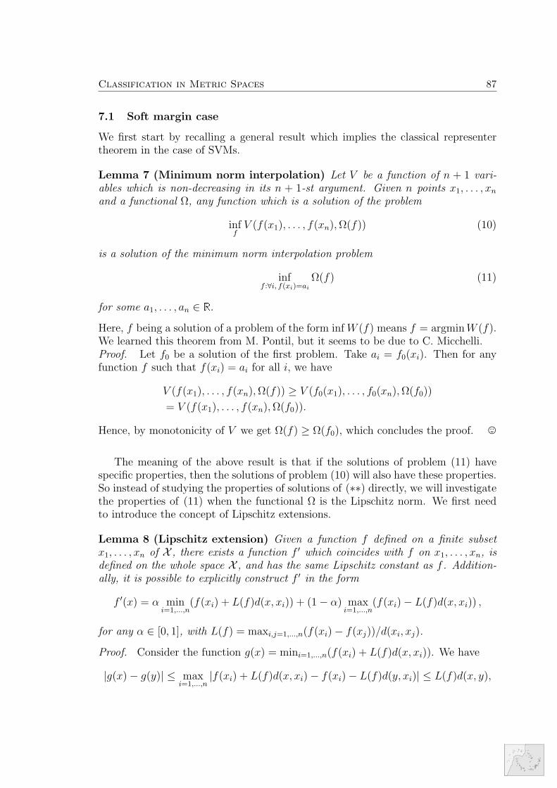
Classification in Metric Spaces 87
7.1 Soft margin case
We first start by recalling a general result which implies the classical representertheorem in the case of SVMs.
Lemma 7 (Minimum norm interpolation) Let V be a function of n + 1 vari-ables which is non-decreasing in its n + 1-st argument. Given n points x1, . . . , xn
and a functional Ω, any function which is a solution of the problem
inffV (f(x1), . . . , f(xn),Ω(f)) (10)
is a solution of the minimum norm interpolation problem
inff :∀i, f(xi)=ai
Ω(f) (11)
for some a1, . . . , an ∈ R.
Here, f being a solution of a problem of the form infW (f) means f = argminW (f).We learned this theorem from M. Pontil, but it seems to be due to C. Micchelli.Proof. Let f0 be a solution of the first problem. Take ai = f0(xi). Then for anyfunction f such that f(xi) = ai for all i, we have
V (f(x1), . . . , f(xn),Ω(f)) ≥ V (f0(x1), . . . , f0(xn),Ω(f0))
= V (f(x1), . . . , f(xn),Ω(f0)).
Hence, by monotonicity of V we get Ω(f) ≥ Ω(f0), which concludes the proof. ,
The meaning of the above result is that if the solutions of problem (11) havespecific properties, then the solutions of problem (10) will also have these properties.So instead of studying the properties of solutions of (∗∗) directly, we will investigatethe properties of (11) when the functional Ω is the Lipschitz norm. We first needto introduce the concept of Lipschitz extensions.
Lemma 8 (Lipschitz extension) Given a function f defined on a finite subsetx1, . . . , xn of X , there exists a function f ′ which coincides with f on x1, . . . , xn, isdefined on the whole space X , and has the same Lipschitz constant as f . Addition-ally, it is possible to explicitly construct f ′ in the form
f ′(x) = α mini=1,...,n
(f(xi) + L(f)d(x, xi)) + (1− α) maxi=1,...,n
(f(xi)− L(f)d(x, xi)) ,
for any α ∈ [0, 1], with L(f) = maxi,j=1,...,n(f(xi)− f(xj))/d(xi, xj).
Proof. Consider the function g(x) = mini=1,...,n(f(xi) + L(f)d(x, xi)). We have
|g(x)− g(y)| ≤ maxi=1,...,n
|f(xi) + L(f)d(x, xi)− f(xi)− L(f)d(y, xi)| ≤ L(f)d(x, y),

88 Chapter III
so that L(g) ≤ L(f). Also, by definition g(xi) ≤ f(xi) + L(f)d(xi, xi) = f(xi).Moreover, if i0 denotes the index where the minimum is achieved in the definitionof g(xi), i.e. g(xi) = f(xi0) + L(f)d(xi, xi0), then by definition of L(f) we haveg(xi) ≥ f(xi0) + (f(xi) − f(xi0)) = f(xi). As a result, for all i = 1, . . . , n we haveg(xi) = f(xi), which also implies that L(g) = L(f).Now the same reasoning can be applied to h(x) = maxi=1,...,n(f(xi)− L(f)d(x, xi)).Since α ∈ [0, 1] we have f ′(xi) = f(xi) for all i. Moreover, L(αg + (1 − α)h) ≤αL(g) + (1− α)L(h) = L(f) and thus L(f ′) = L(f), which concludes the proof. ,
From the above lemma, we obtain an easy way to construct solutions of minimumnorm interpolation problems like (11) with Lipschitz norms, as is expressed in thenext lemma.
Lemma 9 (Solution of the Lipschitz minimal norm interpolation problem)Let a1, . . . , an ∈ R
n, α ∈ [0, 1], L0 = maxi,j=1,...,n(ai − aj)/d(xi, xj), and
fα(x) := α mini=1,...,n
(ai + L0d(x, xi)) + (1− α) maxi=1,...,n
(ai − L0d(x, xi)) .
Then fα is a solution of the minimal norm interpolation problem (11) with Ω(f) =L(f). Moreover, when α = 1/2 then fα is a solution of the minimal norm interpo-lation problem (11) with Ω(f) = ‖f‖L.
Proof. Given that a solution f of (11) has to satisfy f(xi) = ai, it cannot haveL(f) < L0. Moreover, by Lemma 8 fα satisfies the constraints and has L(f) = L0,hence it is a solution of (11) with Ω(f) = L(f).When one takes Ω(f) = ‖f‖L, any solution f of (11) has to have L(f) ≥ L0 and‖f‖∞ ≥ maxi |ai|. The proposed solution fα with α = 1/2 not only satisfies theconstraints fα(xi) = ai but also has L(f) = L0 and ‖f‖∞ = maxi |ai|, which showsthat it is a solution of the considered problem.To prove that ‖f‖∞ = maxi |ai|, consider x ∈ X and denote by i1 and i2 the indiceswhere the minimum and the maximum, respectively, are achieved in the definitionof fα(x). Then one has
f1/2(x) ≤1
2(ai2 + L0d(x, xi2)) +
1
2(ai2 − L0d(x, xi2)) = ai2 ,
and similarly f1/2(x) ≥ ai1 . ,
Now we can formulate a general representer theorem for the soft margin Lipschitzclassifier.
Theorem 10 (Soft margin representer theorem) There exists a solution of thesoft margin Lipschitz classifier (∗∗) in the vector lattice spanned by Dtrain which isof the form
f(x) =1
2min(ai + L0d(x, xi)) +
1
2max(ai − L0d(x, xi))

Classification in Metric Spaces 89
for some real numbers a1, . . . , an with L0 := maxi,j(ai− aj)/d(xi, xj). Moreover onehas ‖f‖L = L(f) = L0.
Proof. The first claim follows from Lemmas 7 and 9. The second claim followsfrom the fact that a solution of (∗∗) satisfies ‖f‖L = L(f). ,
Theorem 10 is remarkable as the space Lip(X ) of possible solutions of (∗∗) containsthe whole vector lattice spanned by D. The theorem thus states that even thoughthe Lipschitz algorithm searches for solutions in the whole lattice spanned by D italways manages to come up with a solution in the sublattice spanned by Dtrain.
7.2 Algorithmic consequences
Theorem 10 states that there always exists a solution f of (∗∗) in a certain paramet-ric form with n parameters a1, ..., an. As a consequence, we can rewrite the originalsoft margin optimization problem
inff∈Lip(X )
L(f) + Cn∑
i=1
ξi subject to yif(xi) ≥ 1− ξi, ξi ≥ 0
in the form
mina1,...,an∈R
maxi,j=1,...,n
i6=j
ai − aj
d(xi, xj)+ C
n∑i=1
ξi subject to yiai ≥ 1− ξi, ξi ≥ 0
which is equivalent to the linear program
mina1,...,an∈R
ρ∈R
ρ+ Cn∑
i=1
ξi subject to yiai ≥ 1− ξi, ξi ≥ 0,ai − aj
d(xi, xj)≥ ρ
To construct a soft margin Lipschitz classifier, we thus have to find the param-eters a1, ..., an which solve this linear program and use the function f defined inTheorem 10 as classifier. Note, however, that in practical applications, the solutionfound by this procedure will usually overfit as it optimizes (∗∗) over the whole classLip(X ). Later we will see how this can be avoided by considering subclasses ofLipschitz functions.
7.3 Hard margin case
The representer theorem for the soft margin case clearly also holds in the hardmargin case, so that there will always be a solution of (∗) in the vector latticespanned by Dtrain. But in the hard margin case, also a different representer theoremis valid. We denote the set of all training points with positive label by X+, the setof the training points with negative label by X−, and for two subsets A,B ⊂ X wedefine d(A,B) := infa∈A,b∈B d(a, b).

90 Chapter III
Theorem 11 (Hard margin representer theorem) Problem (∗) always has asolution which is a linear combination of distances to sets of training points.
To prove this theorem we first need a simple lemma.
Lemma 12 (Optimal Lipschitz constant) The Lipschitz constant L∗ of a solu-tion of (∗) satisfies L∗ ≥ 2/d(X+, X−).
Proof. For a solution f of (∗) we have
L(f) = supx,y∈X
|f(x)− f(y)|d(x, y)
≥ maxi,j=1,...,n
|f(xi)− f(xj)|d(xi, xj)
≥ maxi,j=1,...,n
|yi − yj|d(xi, xj)
=2
minxi∈X+,xj∈X− d(xi, xj)=
2
d(X+, X−).
,
Lemma 13 (Solutions of (∗)) Let L∗ = 2/d(X+, X−). For all α ∈ [0, 1], thefollowing functions solve (∗):
fα(x) := αmini
(yi + L∗d(x, xi) + (1− α) maxi
(yi − L∗d(x, xi))
g(x) :=d(x,X−)− d(x,X+)
d(X+, X−)
Proof. By Lemma 8, fα has Lipschitz constant L∗ and satisfies fα(xi) = yi. More-over, it is easy to see that yig(xi) ≥ 1. Using the properties of Lipschitz constantsstated in Section 5 and the fact that the function d(x, ·) has Lipschitz constant 1 wesee that L(g) ≤ L∗. Thus fα and g are solutions of (∗) by Lemma 12. ,
The functions fα and g lie in the vector lattice spanned by Dtrain. As g is a linearcombination of distances to sets of training points we have proved Theorem 11.
It is interesting to have a closer look at the functions of Lemma 13. The functionsf0 and f1 are the smallest and the largest functions, respectively, that solve problem(∗) with equality in the constraints: any function f that satisfies f(xi) = yi and hasLipschitz constant L∗ satisfies f0(x) ≤ f(x) ≤ f1(x). The functions g and f1/2 areespecially remarkable:
Lemma 14 (1-nearest neighbor classifier) The functions g and f1/2 defined abovehave the sign of the 1-nearest neighbor classifier.

Classification in Metric Spaces 91
Proof. It is obvious that g(x) > 0 ⇐⇒ d(x,X+) < d(x,X−) and g(x) < 0 ⇐⇒d(x,X+) > d(x,X−). For the second function, we rewrite f1/2 as follows:
f1/2(x) =1
2( min(L∗d(x,X+) + 1, L∗d(x,X−)− 1)
−min(L∗d(x,X+)− 1, L∗d(x,X−) + 1)) .
Consider x such that d(x,X+) ≥ d(x,X−). Then d(x,X+) + 1 ≥ d(x,X−)− 1 andthus
f1/2(x) =1
2
(L∗d(x,X−)− 1−min(L∗d(x,X+)− 1, L∗d(x,X−) + 1)
)≤ 0 .
The same reasoning applies to the situation d(x,X+) ≤ d(x,X−) to yield f1/2(x) ≥ 0in this case. ,
Note that g needs not reach equality in the constraints on all the data points,whereas the function f1/2 always satisfies equality in the constraints. Lemma 14has the surprising consequence that according to Section 6, the 1-nearest neighborclassifier actually is a large margin classifier.
7.4 Negative results
So far we have proved that (∗) always has a solution which can be expressed asa linear combination of distances to sets of training points. But maybe we evenget a theorem stating that we always find a solution which is a linear combinationof distance functions to single training points? Unfortunately, in the metric spacesetting such a theorem is not true in general. This can be seen by the followingcounterexample:
Example 1 Assume four training points x1, x2, x3, x4 with distance matrix
D =
0 2 1 12 0 1 11 1 0 21 1 2 0
and label vector y = (1, 1,−1,−1). Then the set
f : X → R| yif(xi) ≥ 1, f(x) =4∑
i=1
aid(xi, x) + b
is empty. The reason for this is that the distance matrix is singular and we haved(x1, ·) + d(x2, ·) = d(x3, ·) = d(x4, ·). Hence, in this example, (∗) has no solutionwhich is a linear combination of distances to single training points. But it still hasa solution as linear combination of distances to sets of training points according toTheorem 11.
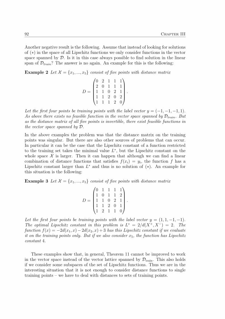
92 Chapter III
Another negative result is the following. Assume that instead of looking for solutionsof (∗) in the space of all Lipschitz functions we only consider functions in the vectorspace spanned by D. Is it in this case always possible to find solution in the linearspan of Dtrain? The answer is no again. An example for this is the following:
Example 2 Let X = x1, ..., x5 consist of five points with distance matrix
D =
0 2 1 1 12 0 1 1 11 1 0 2 11 1 2 0 21 1 1 2 0
.
Let the first four points be training points with the label vector y = (−1,−1,−1, 1).As above there exists no feasible function in the vector space spanned by Dtrain. Butas the distance matrix of all five points is invertible, there exist feasible functions inthe vector space spanned by D.
In the above examples the problem was that the distance matrix on the trainingpoints was singular. But there are also other sources of problems that can occur.In particular it can be the case that the Lipschitz constant of a function restrictedto the training set takes the minimal value L∗, but the Lipschitz constant on thewhole space X is larger. Then it can happen that although we can find a linearcombination of distance functions that satisfies f(xi) = yi, the function f has aLipschitz constant larger than L∗ and thus is no solution of (∗). An example forthis situation is the following:
Example 3 Let X = x1, ..., x5 consist of five points with distance matrix
D =
0 1 1 1 11 0 1 1 21 1 0 2 11 1 2 0 11 2 1 1 0
.
Let the first four points be training points with the label vector y = (1, 1,−1,−1).The optimal Lipschitz constant in this problem is L∗ = 2/d(X+, X−) = 2. Thefunction f(x) = −2d(x1, x)− 2d(x2, x)+3 has this Lipschitz constant if we evaluateit on the training points only. But if we also consider x5, the function has Lipschitzconstant 4.
These examples show that, in general, Theorem 11 cannot be improved to workin the vector space instead of the vector lattice spanned by Dtrain. This also holdsif we consider some subspaces of the set of Lipschitz functions. Thus we are in theinteresting situation that it is not enough to consider distance functions to singletraining points – we have to deal with distances to sets of training points.

Classification in Metric Spaces 93
8 Error Bounds
In this section we compute error bounds for the Lipschitz classifier using Rademacheraverages (recall the definition in Section 1). We will describe two different ways tocompute Rademacher averages for sets of Lipschitz functions. One way is a classicalapproach using entropy numbers and leads to an upper bound on Rn. For thisapproach we always assume that the metric space (X , d) is precompact (i.e., it canbe covered by finitely many balls of radius ε for every ε > 0).The other way is more elegant: because of the definition of ‖ · ‖L and the resultingisometries, the maximum discrepancy of a ‖·‖L-unit ball of Lip(X ) is the same as ofthe corresponding unit ball in AE(X0)
′. Hence it will be possible to express Rn asthe norm of an element of the Arens-Eells space. This norm can then be computedvia bipartite minimal matching. In the following, B always denotes the unit ball ofthe considered function space.
8.1 The duality approach
The main insight to compute the maximum discrepancy by the duality approach isthe following observation:
sup‖f‖L≤1
|n∑
i=1
f(xi)− f(x′i)| = sup‖Tf‖≤1
|n∑
i=1
Tfmxi− Tfmx′i
| =
= sup‖Tf‖≤1
|〈Tf ,n∑
i=1
mxi−mx′i
〉| = ‖n∑
i=1
mxix′i‖AE
Applying this to the definition of the maximum discrepancy immediately yields
Rn(B) =1
nE‖
n∑i=1
mXiX′i‖AE. (12)
As we already explained in Section 5, the norm ‖∑n
i=1mXiX′i‖AE can be inter-
preted as the costs of a minimal bipartite matching between X1, . . . , Xn andX ′
1, . . . , X′n. To compute the right hand side of (12) we need to know the ex-
pected value of random instances of the bipartite minimal matching problem, wherewe assume that the points Xi and X ′
i are drawn iid from the sample distribution.In particular we want to know how this value scales with the number n of pointsas this indicates how fast we can learn. This question has been solved for somespecial cases of random bipartite matching. Let the random variable Cn describethe minimal bipartite matching costs for a matching between the points X1, . . . , Xn
and X ′1, . . . , X
′n drawn iid according to some distribution P . In Dobric and Yukich
(1995) it has been proved that for an arbitrary distribution on the unit square of Rd
with d ≥ 3 we have limCn/(nd−1/d) = c > 0 a.s. for some constant c. The upper
bound ECn ≤ c√n log n for arbitrary distributions on the unit square in R
2 waspresented in Talagrand (1992). These results, together with Equation (12), lead tothe following maximum discrepancies:

94 Chapter III
Theorem 15 (Maximum discrepancy of unit ball of Lip([0, 1]d)) Let X = [0, 1]d ⊂R
d with the Euclidean metric. Then the maximum discrepancy of the ‖ · ‖L-unit ballB of Lip(X ) satisfies
Rn(B) ≤ c2√
log n/√n for all n ∈ N if d = 2
limn→∞
Rn(B) d√n = cd > 0 if d ≥ 3
where cd (d ≥ 2) are constants which are independent of n but depend on d.
Note that this procedure gives (asymptotically) exact results rather than upperbounds in cases where we have (asymptotically) exact results on the bipartite match-ing costs. This is for example the case for cubes in R
d, d ≥ 3 as Dobric and Yukich(1995) gives an exact limit result, or for R2 with the uniform distribution.
8.2 Generalized entropy bound
Recall that the covering number N(X , ε, d) of a totally bounded metric space (X , d)is the smallest number of balls of radius ε with centers in X which can cover X com-pletely. A classical theorem of Dudley (1987) bounds the Rademacher complexityin terms of covering numbers:
Theorem 16 (Classical entropy bound) For every class F of functions thereexists a constant C such that
Rn(F) ≤ C√n
∫ ∞
0
√logN(F , u, L2(µn)) du
where µn is the empirical distribution of the sample.
When we want to apply this bound to Lipschitz function classes in the nextsection we come upon the problem that the integral on the right hand side divergesin some situation. To avoid this we will now prove an adapted version of the entropybound where this problem does not occur:
Theorem 17 (Generalized entropy bound) Let F be a class of functions andX1, . . . , Xn iid sample points with empirical distribution µn. Then, for every ε > 0,
Rn(F) ≤ 2ε+4√
2√n
∫ ∞
ε/4
√logN(F , u, L2(µn)) du.
The idea of the proof of Theorem 17 is the following. Instead of bounding theRademacher complexity on the whole set of functions F , we first consider a maxi-mal ε-separating subset Fε of F . This is a maximal subset such that all its pointshave distance at least ε to each other. To this special set we will then apply theclassical entropy bound. Then we will estimate how much we loose by this procedure.
The following lemma can be found as Lemma 3.10 in Bousquet (2002) (for thedefinition of a separable process see also van der Vaart and Wellner 1996).

Classification in Metric Spaces 95
Lemma 18 (ε-separations of an empirical process) Let Zt; t ∈ T be a sep-arable stochastic process satisfying for λ > 0 the increment condition
∀s, t ∈ T : E(eλ(Zt−Zs)
)≤ eλ2c2d2(s,t)/2.
Let ε ≥ 0 and δ > 0. If ε > 0, let Tε denote a maximal ε-separated subset of T andlet Tε = T otherwise. Then for all t0,
E
(sup
t∈Tε,d(t,t0)≤δ
Zt − Zt0
)≤ 4
√2c
∫ δ/2
ε/4
√logN(T, u, d)du.
To apply this lemma to the Rademacher complexity of a function class F , we choosethe index set T = F , the fixed index t0 = f0 for some f0 ∈ F , the empirical processZf = 1
n
∑σif(Xi), and δ → ∞. Note that the Rademacher complexity satisfies
the increment condition of Lemma 18 with respect to the L2(µn)–distance withconstant c =
√n. Moreover, observe that E(supt Zt − Zt0) = E(supt Zt) − E(Zt0)
and E(Zt0) = E( 1n
∑σif0(Xi)) = 0. Together with the symmetry of the distribution
of Zf we thus get the next lemma:
Lemma 19 (Entropy bound for ε-separations) Let (Xi)i=1,...,n be iid trainingpoints with empirical distribution µn, F an arbitrary class of functions, and Fε amaximal ε-separating subset of F with respect to L2(µn)- norm. Then
E
(supf∈Fε
1
n|∑
i
σif(Xi)|∣∣∣X1, . . . , Xn
)≤ 4
√2√n
∫ ∞
ε/4
√logN(F , u, L2(µn)) du.
With this lemma we achieved that the integral over the covering numbers startsat ε/4 instead of 0 as it is the case in Theorem 16. The price we pay is that thesupremum on the left hand side is taken over the smaller set Fε instead of the wholeclass F . Our next step is to bound the mistake we make by this procedure.
Lemma 20 Let F be a class of functions and Fε a maximal ε-separating subset ofF with respect to ‖ · ‖L2(µn). Then |Rn(F)−Rn(Fε)| ≤ 2ε.
Proof. We want to bound the expression
|Rn(F)−Rn(Fε)| = E1
n
∣∣∣∣supf∈F
|∑
σif(Xi)| − supf∈Fε
|∑
σif(Xi)|∣∣∣∣.
First look at the expression inside the expectation, assume that the σi and Xi arefixed and that supf∈F |
∑σif(xi)| = |
∑σif
∗(xi)| for some function f ∗ (if f ∗ doesnot exist we additionally have to use a limit argument). Let fε ∈ Fε such that‖f ∗ − fε‖L2(µn) ≤ 2ε. Then,
1
n
∣∣∣∣supf∈F
|∑
σif(xi)| − supf∈Fε
|∑
σif(xi)|∣∣∣∣ ≤ 1
n
∣∣∣|∑ σif∗(xi)| − |
∑σifε(xi)|
∣∣∣≤ 1
n
∣∣∣∑ σi(f∗(xi)− fε(xi))
∣∣∣ ≤ ‖f ∗ − fε‖L1(µn) ≤ ‖f ∗ − fε‖L2(µn) ≤ 2ε

96 Chapter III
As this holds conditioned on all fixed values of σi and Xi we get the same for theexpectation. This proves the lemma. ,
To prove Theorem 17 we now combine lemmas 19 and 20.
8.3 Covering number approach
To apply this theorem we need to know covering numbers of spaces of Lipschitzfunctions. This can be found for example in Kolmogorov and Tihomirov (1961),pp.353–357.
Theorem 21 (Covering numbers for Lipschitz function balls) For a totallybounded metric space (X , d) and the unit ball B of (Lip(X ), ‖ · ‖L),
2N(X ,4ε,d) ≤ N(B, ε, ‖ · ‖∞) ≤(
2
⌈2 diam(X )
ε
⌉+ 1
)N(X , ε4,d)
.
If, in addition, X is connected and centered (i.e., for all subsets A ⊂ X withdiam(A) ≤ 2r there exists a point x ∈ X such that d(x, a) ≤ r for all a ∈ A),
2N(X ,2ε,d) ≤ N(B, ε, ‖ · ‖∞) ≤(
2
⌈2 diam(X )
ε
⌉+ 1
)· 2N(X , ε
2,d).
Combining Theorems 17 and 21 and using N(F , u, L2(µn)) ≤ N(F , u, ‖ · ‖∞) nowgives a bound on the Rademacher complexity of balls of Lip(X ):
Theorem 22 (Rademacher complexity of unit ball of Lip(X )) Let (X , d) be atotally bounded metric space with diameter diam(X ) and B the ball of Lipschitzfunctions with ‖f‖L ≤ 1. Then, for every ε > 0,
Rn(B) ≤ 2ε+4√
2√n
∫ 4 diam(X )
ε/4
√N(X , u
4, d) log
(2
⌈2 diam(X )
u
⌉+ 1
)du.
If, in addition, X is connected and centered, we have
Rn(B) ≤ 2ε+4√
2√n
∫ 2 diam(X )
ε/4
√N(X , u
2, d) log 2 + log(2
⌈2 diam(X )
u
⌉+ 1) du.
In our framework this is a nice result as the bound on the complexity of balls ofLip(X ) only uses the metric properties of the underlying space X .
Now we want to compare the results of Theorems 15 and 22 for two simpleexamples.

Classification in Metric Spaces 97
Example 4 (d-dimensional unit square, d ≥ 3) Let X = [0, 1]d ⊂ Rd, d ≥ 3,
with the Euclidean metric ‖·‖2. This is a connected and centered space. In Theorem15 we showed that Rn(B) asymptotically scales as 1/ d
√n, and this result cannot be
improved. Now we want to check whether Theorem 22 achieves a similar scaling rate.To this end we choose ε = 1/ d
√n (as we know that we cannot obtain a rate smaller
than this) and use that the covering numbers of X have the form N(X , ε, ‖ · ‖2) =c/εd (e.g., page 1 of Mendelson and Vershynin, 2003). After evaluating the secondintegral of Theorem 22 we find that Rn(B) indeed scales as 1/ d
√n.
Example 5 (2-dimensional unit square) Let X = [0, 1]2 ⊂ R2 with the Eu-
clidean metric. Applying Theorem 22 similar to Example 4 yields a bound on Rn(B)that scales as log n/
√n.
In case of Example 4 the scaling behavior of the upper bound on Rn(B) obtained bythe covering number approach coincides with the exact result for Rn(B) derived inTheorem 15. In case of Example 5 the covering number result log n/
√n is slightly
worse than the result√
log(n)/√n obtained in Theorem 15.
8.4 Complexity of Lipschitz RBF classifiers
In this section we want to derive a bound for the Rademacher complexity of radialbasis function classifiers of the form
Frbf := f : X → R| f(x) =l∑
k=1
akgk(d(pk, x)), gk ∈ G, l <∞, (13)
where pk ∈ X , ak ∈ R, and G ⊂ Lip(X ) is a (small) set of ‖ · ‖∞-bounded Lipschitzfunctions on R whose Lipschitz constants are bounded from below by a constantc > 0. As an example, consider G = g : R→ R| g(x) = exp(−x2/σ2), σ ≥ 1. Thespecial case G = id corresponds to the function class which is used by the linearprogramming machine. It can easily be seen that the Lipschitz constant of an RBFfunction satisfies L(
∑k akgk(d(pk, ·))) ≤
∑k |ak|L(gk). We define a norm on Frbf by
‖f‖rbf := inf
∑k
|ak|L(gk); f =∑
k
akgk(d(pk, ·))
and derive the Rademacher complexity of a unit ball B of (Frbf , ‖·‖rbf ). Substitutingak by ck/L(gk) in the expansion of f we get
supf∈B
|n∑
i=1
σif(xi)| = sup∑|ak|L(gk)≤1,pk∈X ,gk∈G
|n∑
i=1
σi
l∑k=1
akgk(d(pk, xi))|
= sup∑|ck|≤1,pk∈X ,gk∈G
|n∑
i=1
σi
l∑k=1
ckL(gk)
gk(d(pk, xi))|

98 Chapter III
= sup∑|ck|≤1,pk∈X ,gk∈G
|l∑
k=1
ck
n∑i=1
σi1
L(gk)gk(d(pk, xi))|
= supp∈X ,g∈G
|n∑
i=1
σi1
L(g)g(d(p, xi))| (14)
For the last step observe that the supremum in the linear expansion in the secondlast line is obtained when one of the ck is 1 and all the others are 0. To proceed weintroduce the notations hp,g(x) := g(d(p, x))/L(g), H := hp,g; p ∈ X , g ∈ G, andG1 := g/L(g); g ∈ G. We rewrite the right hand side of Equation (14) as
supp∈X ,g∈G
|n∑
i=1
σi1
L(g)g(d(p, xi))| = sup
hp,g∈H|
n∑i=1
σihp,g(xi)|
and thus obtain Rn(B) = Rn(H). To calculate the latter we need the following:
Lemma 23 N(H, 2ε, ‖ · ‖∞) ≤ N(X , ε, d)N(G1, ε, ‖ · ‖∞).
Proof. First we observe that for hp1,g1 , hp2,g2 ∈ H
‖hp1,g1 − hp2,g2‖∞ = supx∈X
|g1(d(p1, x))
L(g1)− g2(d(p2, x))
L(g2)|
≤ supx∈X
(|g1(d(p1, x))
L(g1)− g1(d(p2, x))
L(g1)|+ | |g1(d(p2, x))
L(g1)− g2(d(p2, x))
L(g2)|)
≤ supx∈X
|d(p1, x)− d(p2, x)|+ ‖ g1
L(g1)− g2
L(g2)‖∞
≤ d(p1, p2) + ‖ g1
L(g1)− g2
L(g2)‖∞ =: dH(hp1,g1 , hp2,g2) (15)
For the step from the second to the third line we used the Lipschitz property of g1.Finally, it is easy to see that N(H, 2ε, dH) ≤ N(X , ε, d)N(G1, ε, ‖ · ‖∞). ,
Plugging Lemma 23 in Theorem 17 yields the following Rademacher complexity:
Theorem 24 (Rademacher complexity of unit ball of Frbf) Let B be theunit ball of (Frbf , ‖ · ‖rbf ), G1 the rescaled functions of G as defined above, andw := maxdiam(X , d), diam(G1, ‖ · ‖∞). Then, for every ε > 0,
Rn(B) ≤ 2ε+4√
2√n
∫ w
ε/4
√logN(X , u
2, d) + logN(G1,
u
2, ‖ · ‖∞) du.
This theorem is a huge improvement compared to Theorem 22 as instead of thecovering numbers we now have log-covering numbers in the integral. As an exampleconsider the linear programming machine on X = [0, 1]d. Because of G = id,the second term in the square root vanishes, and the integral over the log-coveringnumbers of X can be bounded by a constant independent of ε. As result we obtainthat in this case Rn(B) scales as 1/
√n.

Classification in Metric Spaces 99
9 Choosing subspaces of Lip(X )
So far we always considered the isometric embedding of the given metric space intothe Arens-Eells space and discovered many interesting properties of this embed-ding. But there exist many different isometric embeddings which could be usedinstead. Hence, the construction of embedding the metric space isometrically intosome Banach space and then using a large margin classifier in this Banach space isalso possible with different Banach spaces than the Arens-Eells space. For example,Hein and Bousquet (2003) used the Kuratowski embedding, which maps a metricspace X isometrically in the space of continuous functions (C(X ), ‖·‖∞) (see Exam-ple 6 below). Now it is a natural question whether there are interesting relationshipsbetween large margin classifiers constructed by the different isometric embeddings,especially with respect to the Lipschitz classifier.
A second question concerns the choice of subspaces of Lip(X ). At the end of Sec-tion 6 we already explained that we have to work on some “reasonable” subspaceof Lipschitz functions to apply the Lipschitz classifier in practice. This is justi-fied by complexity arguments, but does the large margin interpretation still hold ifwe do this? Is there some geometric intuition which could help choosing a subspace?
It will turn out that both questions are inherently related to each other. We willshow that there is a correspondence between embedding X into a Banach space Vand constructing the large margin classifier on V on the one hand, and choosing asubspace F of Lip(X ) and constructing the Lipschitz classifier from F on the otherhand. Ideally, we would like to have a one-to-one correspondence between V and F .In one direction this would mean that we could realize any large margin classifier onany Banach space V with the Lipschitz classifier on an appropriate subspace F ofLipschitz functions. In the other direction this would mean that choosing a subspaceF of Lipschitz functions corresponds to a large margin classifier on some Banachspace V . We could then study the geometrical implications of a certain subspace Fvia the geometric properties of V .
Unfortunately, such a nice one-to-one correspondence between V and F is notalways true, but in many cases it is. We will show that given an embedding intosome vector space V , the hypothesis class of the large margin classifier on V alwayscorresponds to a subspace F of Lipschitz functions (Lemma 28). In general, thiscorrespondence will be an isomorphism, but not an isometry. The other way round,given a subspace F of Lipschitz functions, under some conditions we can constructa vector space V such that X can be isometrically embedded into V and the largemargin classifiers on V and F coincide (Lemma 29).
The key ingredient in this section is the fact that AE(X0) is a free Banach space.The following definition can be found for example in Pestov (1986).

100 Chapter III
Definition 25 (Free Banach space) Let (X0, d, e) be a pointed metric space. ABanach space (E, ‖ · ‖E) is a free Banach space over (X0, d, e) if the following prop-erties hold:
1. There exists an isometric embedding Φ : X0 → E with Φ(e) = 0, and E is theclosed linear span of Φ(X0).
2. For every Banach space (V, ‖ · ‖V ) and every Lipschitz map Ψ : X0 → V withL(Ψ) = 1 and Ψ(e) = 0 there exists a linear operator T : E → V with ‖T‖ = 1such that T Φ = Ψ.
It can be shown that the free Banach space over (X , d, e) always exists and isunique up to isomorphism (cf. Pestov, 1986).
Lemma 26 (AE is a free Banach space) For any pointed metric space(X0, d, e), AE(X0) is a free Banach space.
Proof. Property (1) of Definition 25 is clear by construction. For a proof of prop-erty (2), see for example Theorem 2.2.4 of Weaver (1999). ,
We are particularly interested in the case where the mapping Ψ : X0 → V ofDefinition 25 is an isometric embedding of X0 into some vector space V . Firstlywe want to find out under which conditions its dual V ′ is isometric isomorphic tosome subspace F of Lip(X ). Secondly, given a subspace F of Lip(X ) the question iswhether there exists a Banach space V such that X0 can be embedded isometricallyinto V and simultaneously V ′ is isometric isomorphic to F . Both questions will beanswered by considering the mapping T of Definition 25 and its adjoint T ′. Thefollowing treatment will be rather technical, and it might be helpful to have Figure1 in mind, which shows which relations we want to prove.
X0
AE’ = Lip
V’ = F
T’
exist?V, ψ?
isometry T’ exists
?AE
V
φ
ψ
T
exists T’ isometry?isometry ψ
Figure 1: Relations between Banach spaces and subspaces of Lipschitz functions. The leftpart shows the commutative diagram corresponding to the free Banach space property ofAE(X0). The right part shows the adjoint mapping T ′ of T . The dotted arrows in themiddle show the relationships we want to investigate.
Now we want to go into detail and start with the first question. For simplicity,we make the following definition.

Classification in Metric Spaces 101
Definition 27 (Dense isometric embedding) Let (X0, d) a metric space and Va normed space. A mapping Ψ : X0 → V is called a dense isometric embedding ifΨ is an isometry and if V is the norm-closure of spanΨ(x);x ∈ X0.
Lemma 28 (Construction of F for given V ) Let (X0, d) be a pointed metricspace, (V, ‖ · ‖V ) a normed space and Ψ : X0 → V a dense isometric embedding.Then V ′ is isomorphic to a closed subspace F ⊂ Lip0(X0), and the canonical injec-tion i : F → Lip0(X0) satisfies ‖i‖ ≤ 1.
Proof. Recall the notation mx := Φ(x) from Section 6 and analogously denotevx := Ψ(x). Let T : AE(X0) → V the linear mapping with T Φ = Ψ as in Definition25. As Ψ is an isometry, T satisfies ‖T‖ = 1, and maps AE(X0) on some dense sub-space of V . Consider the adjoint T ′ : V ′ → AE(X0)
′. It is well known (e.g., Chapter4 of Rudin, 1991) that ‖T‖ = ‖T ′‖ and that T ′ is injective iff the range of T is dense.Thus, in our case T ′ is injective. As by construction also 〈Tmx, v
′〉 = 〈T ′v′,mx〉, wehave a unique correspondence between the linear functions in V ′ and some subspaceF := T ′V ′ ⊂ AE(X0)
′: for g ∈ V ′ and f = T ′g ∈ Lip0(X0) we have g(vx) = f(mx)for every x ∈ X0. The canonical inclusion i corresponds to the adjoint T ′. ,
Lemma 28 shows that the hypothesis space V ′ constructed by embedding Xinto V is isomorphic to a subset F ⊂ Lip0(X0). But it is important to note thatthis isomorphism is not isometric in general. Let g ∈ V ′ and f ∈ Lip0(X0) becorresponding functions, that is f = T ′g. Because of ‖T ′‖ = 1 we know that‖f‖AE′ ≤ ‖g‖V , but in general we do not have equality. This means that themargins ‖g‖V ′ and ‖f‖AE′ of corresponding functions are measured with respect todifferent norms and might have different sizes. As a consequence, the solutions ofthe two large margin problems
ming∈V ′
‖g‖V ′ subject to yig(vxi) ≥ 1
and
minf∈F
‖f‖L subject to yif(xi) ≥ 1
might be different, even though the sets of feasible functions are the same in bothcases.
To illustrate this we will consider two examples. The first one shows how thelarge margin classifier in V can give different results than the one constructed byusing the corresponding subspace for the Lipschitz classifier. In the second examplewe show a situation where both classifiers coincide.
Example 6 (Kuratowski embedding) Let (X , d) be an arbitrary compact metricspace and (C(X ), ‖ · ‖∞) the space of continuous functions on X . Define Ψ : X →C(X ), x 7→ d(x, ·). This mapping is an isometric embedding called Kuratowski

102 Chapter III
embedding, and it has been used in Hein and Bousquet (2003) to construct a largemargin classifier. We want to compare the large margin classifiers resulting from theKuratowski embedding and the embedding in the Arens-Eells space. As an exampleconsider the finite metric space X = x1, ..., x4 with distance matrix
D =
0 5 3 65 0 4 13 4 0 56 1 5 0
.
Let V = spand(x, ·); x ∈ X ⊂ C(X ), endowed with the norm ‖ · ‖∞. V isa 4-dimensional vector space. Let V ′ its dual space. Via the mapping T ′, eachlinear operator g ∈ V ′ corresponds to the linear operator f ∈ Lip0(X0) with f(xi) =〈g, d(xi, ·)〉 =: ci. Now we want to compare the norms of g in V ′ and f in Lip(X ).Thenorm of g in V ′ can be computed as follows:
‖g‖V ′ = sup〈g, v〉 : v ∈ V, ‖v‖V ≤ 1
= sup〈g,4∑
i=1
aid(xi, ·)〉 : ai ∈ R, ‖4∑
i=1
aid(xi, ·)‖∞ ≤ 1
= sup4∑
i=1
aici : ai ∈ R, −1 ≤4∑
i=1
aid(xi, xj) ≤ 1 for all j = 1, ..., 4 .
For given function g ∈ V ′ (that is, for given values ci) this norm can be computed bya linear program. Consider the two functions g1, g2 ∈ V ′ with values on x1, x2, x3, x4
given as (−1,−1,−1,−1) and (1, 0, 1, 0), respectively, and let f1, f2 ∈ Lip0(X0) bethe corresponding Lipschitz functions. Then we have ‖f1‖L = 0.166 < 0.25 = ‖f2‖L
and ‖g1‖V ′ = 0.366 > 0.28 = ‖g2‖V ′. So the norms ‖ · ‖V ′ and ‖ · ‖L do notcoincide, and moreover there is no monotonic relationship between them. If themaximal margin algorithm had to choose between functions f1 and f2, it would cometo different solutions, depending whether the underlying norm is ‖ · ‖V ′ as for thelarge margin classifier in V ′ or ‖ · ‖L as for the Lipschitz classifier in T ′V ′.
Example 7 (Normed space) Let (X , ‖ · ‖X ) be a normed vector space with dual(X ′, ‖ · ‖X ′). As the norm of linear functions coincides with their Lipschitz constant,X ′ is isometrically isomorphic to a subspace of Lip0(X0). This means that it makesno difference whether we construct a large margin classifier on the normed space Xdirectly or ignore the fact that X is a normed space, embed X into AE(X0) and thenconstruct the Lipschitz classifier on AE(X0) with the subspace T ′X ′. We alreadymentioned this fact in Section 6 when we stated that the SVM solution is the sameone as the Lipschitz classifier on X ′.
Now we want to investigate our second question: given some subspace F ⊂Lip0(X0), is F the dual space of some Banach space V such that X0 can be embeddedisometrically into V and V ′ ' F? To answer this question we have to deal with some

Classification in Metric Spaces 103
technical problems. First of all, F has to possess a pre-dual, that is a vector spaceV whose dual V ′ coincides with F . In general, not every Banach space possessesa pre-dual, and if it exists, it needs not be unique. Secondly, it turns out that thecanonical injection T ′ : F → Lip0(X0) has to have a pre-adjoint, that is a mappingT : AE(X0) → V whose adjoint coincides with T ′. Pre-adjoints also not always exist.In general, neither the existence of a pre-dual nor the existence of pre-adjoints areeasy to prove. One situation where both can be handled is the case where F isclosed under pointwise convergence:
Lemma 29 (Construction of V for given F ) Let X0 be a bounded metric space,and F a subspace of (Lip0(X0), L(·)) which is closed under pointwise convergence andsatisfies the condition
supf∈F,L(f)≤1
|f(x)− f(y)| = d(x, y) (16)
for all x, y ∈ X0. Then there exists a normed space V such that X0 can be isometri-cally embedded into V and its dual V ′ is isometrically isomorphic to F .
Before we can start with the proof we need two more definitions: Let M be asubspace of some Banach space V and N a subspace of the dual space V ′. Then theannihilator M⊥ and the pre-annihilator ⊥N are defined as M⊥ = T ∈ V ′; Tm =0 for all m ∈ M and ⊥N = e ∈ V ; Te = 0 for all T ∈ N. As the proof is a bittechnical, we refer to Megginson (1998) for background reading.
Proof. For a bounded metric space X0, the topology of pointwise convergence onLip0(X0) coincides with its weak* topology. Thus by assumption, F is weak*-closed,which implies that ⊥F is a closed subspace of AE(X0). Hence, the quotient spaceV := AE(X0)/
⊥F exists, and there exists an isometric isomorphism between V ′
and (⊥F )⊥. As F is weak*-closed, (⊥F )⊥ = F . So V is a pre-dual of F . Let T ′ :F → Lip0(X0) be the canonical inclusion. It has a pre-adjoint, namely the quotientmapping π : AE(X0) → V . Define the mapping Ψ : X0 → V , x 7→ πmx =: vx. Wehave
〈f, vx〉 = 〈f, πmx〉 = 〈T ′f,mx〉 = 〈f,mx〉 = f(x).
Hence, by assumption (16), Ψ is an isometry:
‖Ψ(x)−Ψ(y)‖V = supf∈F,L(f)≤1
|〈f, vx − vy〉| = supf∈F,L(f)≤1
|f(x)− f(y)| = d(x, y).
,
Lemma 29 gives a nice interpretation of what it means geometrically to choose asubspace F of Lipschitz functions: the Lipschitz classifier with hypothesis space Fcorresponds to embedding X isometrically into the pre-dual V of F and constructingthe large margin classifier on V directly. Condition (16), which F has to satisfy toallow this interpretation, intuitively means that F has to be a “reasonably large”subspace.

104 Chapter III
Example 8 (Linear combination of distance functions) Let F be the sub-space of Lip(X ) consisting of functions of the form f(x) =
∑i aid(xi, x) + b, and
F ⊂ Lip(X ) its closure under pointwise convergence. As norm on F we take theLipschitz constant. On F , condition (16) is satisfied: trivially, we always have ≤in (16), and for given x, y ∈ X , equality is reached for the function f = d(x, ·). Sowe can conclude by Lemma 29 that the Lipschitz classifier on F has the geometricalinterpretation explained above.
10 Discussion
We derived a general approach to large margin classification on metric spaces whichuses Lipschitz functions as decision functions. Although the Lipschitz algorithm,which implements this approach, has been derived in a rather abstract mathemat-ical framework, it boils down to an intuitively plausible mechanism: it looks for adecision function which has a small Lipschitz constant. This agrees with the regu-larization principle that tries to avoid choosing functions with a high variation. Thesolution of the Lipschitz algorithm is well behaved as, by the representer theoremsof Section 7, it can always be expressed by distance functions to training points.For some special cases, the solution corresponds to solutions of other well knownalgorithms, such as the support vector machine, the linear programming machine,or the 1-nearest neighbor classifier. We provide Rademacher complexity bounds forsome of the involved function classes which can be used to bound the generalizationerror of the classifier.
In spite of all those nice properties there are several important questions whichremain unanswered. To apply the Lipschitz algorithm in practice it is important tochoose a suitable subspace of Lipschitz functions as hypothesis space. In Section9 we found a geometrical explanation of what the choice of certain subspaces Fmeans: it is equivalent to using a different isometric embedding of the metric spaceinto some Banach space. But this explanation does not solve the question of whichsubspace we should choose in the end. Moreover, there exist isometric embeddingsin certain Banach spaces which have no such interpretation in terms of subspaces ofLipschitz functions. For example, Hein and Bousquet (2003) studied the Kuratowskiembedding of a metric space into its space of continuous functions to construct alarge margin algorithm. As we explained in Example 6, the large margin classifierresulting from this embedding can be different from the Lipschitz classifier. It is aninteresting question how different embeddings into different Banach spaces shouldbe compared. One way to do this could be comparing the capacities of the inducedfunction spaces. An interesting question in this context is to find the “smallestspace” (for instance, in terms of the Rademacher complexities) in which a givendata space can be embedded isometrically.
There is also a more practical problem connected to the choice of the subspace

Classification in Metric Spaces 105
of Lipschitz functions. To implement the Lipschitz algorithm for a given subspaceof Lipschitz functions, we need to know some way to efficiently compute the Lip-schitz constants of the functions in the chosen subspace. For example, in case ofthe linear programming machine it was possible to bound the Lipschitz constants ofthe functions in the parameterized subspace of functions
∑i aid(xi, ·) + b in terms
of their parameters by∑
i |ai|. But in many cases, there is no obvious parametricrepresentation of the Lipschitz constant of a class of functions. Then it is not clearhow the task of minimizing the Lipschitz constant can be efficiently implemented.
An even more heretic question is whether isometric embeddings should be usedat all. In our approach we adopted the point of view that a meaningful distancefunction between the training points is given by some external knowledge, and thatwe are not allowed to question it. But in practical applications it is often the casethat distances are estimated by some heuristic procedure which might not give asensible result for all the training points. In those cases the paradigm of isometricembedding might be too strong. Instead we could look for bi-Lipschitz embeddingsor low distortion embeddings of the metric space into some Banach space, or eveninto some Hilbert space. We would then loose some (hopefully unimportant) infor-mation on the distances in the metric space, but the gain might consist in a simplerstructure of the classification problem in the target space.
Finally, many people argue that for classification only “local properties” shouldbe considered. One example is the assumption that the data lies on some lowdimensional manifold in a higher dimensional space. In this case, the meaningfulinformation consists of the intrinsic distances between points along the manifold.In small neighborhoods, those distances are close to the distances measured in theenclosing space, but for points which are far away from each other this is not trueany more. In this setting it is not very useful to perform an isometric embedding ofthe metric space into a Banach space as the additional linear structure the Banachspace imposes on the training data might be more misleading than helpful. Here adifferent approach has to be taken, but it is not clear how a large margin algorithmin this setting can be constructed, or even whether in this case the large marginparadigm should be applied at all.


Chapter IV
A Compression Approach toSupport Vector Model Selection
In the last chapters we studied the behavior of machine learning algorithms for afixed similarity or dissimilarity function. The topic of this chapter is how the pa-rameters of a similarity function can be determined from the given training data. Tomake an optimal choice of parameters we first have to decide which learning algo-rithm we want to use. In this chapter this will be simply a support vector machinewith Gaussian kernels. For this algorithm we will then interpret the constructedclassifiers with methods from information theory and data compression. This willlead to an implementation of Ockham’s razor: we choose the set of parameters suchthat the resulting classifier is as “simple to describe” as possible. This will be doneby constructing “compression coefficients” which measure how well the informationabout the training labels can be encoded with the help of a given hyperplane. Themain idea is to relate the coding precision to geometrical concepts such as the widthof the margin or the shape of the data in the feature space. These compressioncoefficients will then be tested in model selection experiments. As a result we findthat compression coefficients can fairly accurately predict the parameters for whichthe test error is minimized.
1 Model selection via compression bounds
1.1 Model selection
In statistical learning theory, a model M is simply a class of functions. For a givenmodel, the learning step consists in choosing the function from the model which bestexplains our training data. In many applications, it is not clear from the beginningwhich kind of function class is appropriate to model the data. If the model is toosimple, it might not contain a good classifier at all. If the model is too complex it isvery likely that we will overfit. The term model selection now refers to the problemof choosing a model from a given class of models (Mi)i∈I which is well suited to our
108 Chapter IV
training data.
In the case of hard margin support vector machines, the model class only de-pends on the kernel function we choose. Each kernel function k gives rise to amodel Mk :=
∑i aik(xi, ·) + b; ai, b ∈ R. In this context, model selection is
the problem of choosing a good kernel function. Often we already know whatthe type of the kernel function we want to use, for example the Gaussian kernelkσ(x, y) = exp(−‖x− y‖2/σ2). Here the class of models is a parametric class, eachparticular value of σ corresponding to some model Mσ. Model selection then re-duces to choosing the best parameter σ. For the soft margin support vector machine,additionally to the kernel function we also have to determine the soft margin pa-rameter C (recall the soft margin optimization problem in Section III.3). Choosingboth σ and C is the model selection problem we will study in this chapter.
One standard way to perform model selection is to use model complexity es-timates and generalization bounds. The model complexity assesses “how large” afunction class is. Examples for such complexity measures are covering numbers ofthe function space, the VC dimension, or the Rademacher complexity. The gener-alization bounds derived in statistical learning theory usually have the form
R(f) ≤ Remp(f) + C(F)
where F is the given function class, C some complexity measure of it, and f a func-tion in F (which might be chosen by a certain algorithm). Given the training data,such a bound can be used for model selection by choosing the model F which min-imizes the right hand side minf∈F Remp(f) + C(F) over the given set of models. Tomake this feasible in practice, the complexity measure C has to be easy to compute.Often this is not the case, for example if the complexity is expressed in terms ofcovering numbers of the function space.
1.2 Data compression and learning
One particular measure of complexity of a function class can be obtained by datacompression arguments. The general idea is that the complexity of a model (withrespect to the given training data) is low if the information contained in the trainingdata can be compressed effectively with the help of the model. Following the conven-tions in the compression literature, models will also be called hypothesis spaces inthe following, and the terms “classifier” and “hypothesis” will be used synonymously.
In the framework of Vapnik (1998, Section 6.2), classifiers are used to constructcodes that can transmit the labels y1, ..., yn of a set of training patterns x1, ..., xn.What those codes essentially do is to tell the receiver which classifier h from a givenhypotheses class he should use to reconstruct the training labels from the training

A Compression Approach to Model Selection 109
patterns (this is described in detail in Section 2). For such a code, the compressioncoefficient C(h) is defined as
C(h) :=number of bits to code y1, ..., yn using h
n. (1)
The denominator corresponds to the number of bits we need to transmit the uncom-pressed binary vector (y1, ..., yn). The numerator tells us how many bits we need totransmit the same information using the code constructed with help of classifier h.Hence, the compression coefficient is a number between 0 and 1 which describes howefficient the code works. Intuitively, if the compression coefficient C(h) is small, h isa “simple” hypothesis which we expect not to overfit too much and hence to have asmall generalization error. This belief is supported by the following theorem, whichbounds the risk R(h) of a classifier h with respect to the 0-1-loss in terms of thecompression coefficient:
Theorem 1 (Section 6.2 in Vapnik 1998) With probability at least 1−η over nrandom training points drawn iid according to the unknown distribution P , the riskR(h) of classifier h is bounded by
R(h) ≤ 2 ln(2)C(h)− ln(η)
n
simultaneously for all classifiers h in a finite hypotheses set.
This bound has the disadvantage that it is only valid in the restricted setting wherethe hypotheses space is finite and independent of the training data.
A different bound that directly works in the coding setting has been statedby Blum and Langford (2003). Their setting is slightly different from the one ofVapnik. For a given set of training and test points, the sender constructs a code hthat transmits the labels of both training and test points. Rtest is then defined asthe error which the code h makes on the given test set.
Theorem 2 (Corollary 3 in Blum and Langford 2003) With probability at least1 − η over n random training points and n random test points drawn iid accordingto the unknown distribution P , and for all codes h which encode the training labelswithout error, the error Rtest(h) on the test set satisfies
Rtest(h) ≤ C(h)− ln η
n.
The advantage of this bound is that the problem of data dependency does not oc-cur. It is proved within the coding framework, without assuming a fixed hypothesesspace. It is valid for all codes, as long as receiver and sender agree on how thecode works before the sender knows the training data. In particular, the codes maydepend on the training data in some predefined way, as it will be the case for thecodes we are going to construct.

110 Chapter IV
In general it is well-known that there is a tight connection between learning andcoding. In some way, the process of learning corresponds to finding efficient codes todescribe the input space. In the minimum description length (MDL) framework (cf.Barron et al., 1998, and references therein), this connection is made explicit. TheMDL principle states that, among a given set of hypotheses, one should choose thehypothesis that achieves the shortest description of the training data. Intuitively,this seems to be a reasonable choice: by Shannon’s source coding theorem (cf.Cover and Thomas, 1991) we know that an efficient code is closely related to thedata generating distribution. Moreover, an easy-to-describe hypothesis is less likelyto overfit than a more complicated one.
There are several connections between the MDL principle and other learningmethods. It can be shown that selecting the hypothesis with the highest posteriorprobability in a Bayesian setting is equivalent to choosing the hypothesis with theshortest code (cf. Hansen and Yu, 2001). For SVMs, the compression scheme ap-proach of Floyd and Warmuth (1995), which describes the generalization of a learn-ing algorithm by its ability to reduce the training set to a few important points, leadsto a bound in terms of the number of support vectors. Combining this result withlarge margin bounds yields the sparse margin bound of Herbrich et al. (2000). InMcAllester (1999), a PAC-Bayesian bound for learning algorithms was derived. Fora given prior distribution P on the hypotheses space, it bounds the generalizationerror essentially by the quantity − lnP (U)/m, where U is the subset of hypothesesconsistent with the training examples. Intuitively we can argue that, according toShannon’s theorem, − lnP (U) corresponds to the length of the shortest code forthis subset.
In the following we want to explore whether the connection between statisticallearning theory and data compression is only of theoretical interest or whether itcan also be exploited for practical purposes. Our idea is to use the compressioncoefficient bounds above for model selection. The main work will consist in find-ing a way to actually compute compression coefficients for a given model and giventraining data. The special case we will consider is model selection for soft mar-gin SVMs. The first part of the work (Section 2) will consist in using hyperplaneslearned by SVMs to construct codes for the training labels. Those codes work byencoding the direction of the separating hyperplane. To make them efficient, wewill use geometric concepts such as the size of the margin or the shape of the datain the feature space, and sparsity arguments. The main insight of this section ison how to transform those geometrical concepts into an actual code for labels. Inthe end we obtain compression coefficients that contain quantities already known tobe meaningful in the statistical learning theory of SVMs, such as the radius-marginterm R2/ρ2, the eigenvalues of the kernel matrix, and the number of support vec-tors. In the second part (Section 3) we then test the model selection performance ofour compression coefficients on benchmark data sets. We find that the compressioncoefficients perform comparable or better than several standard bounds.

A Compression Approach to Model Selection 111
Now we want to establish some notation for this chapter. For a given kernelfunction k we denote the kernel matrix by K := (k(xi, xj))i,j=1,...,n. We will denoteits eigenvalues by λ1, ..., λn, where the λi are sorted in non-increasing order. Lateron we will also consider the kernel matrix KSV restricted to the span of the supportvectors. To define it, let xi1 , ..., xis ⊂ x1, ..., xn the set of support vectors,SV := k | xk ∈ spanxi1 , ..., xis the indices of those training points which are inthe subspace spanned by the support vectors. Then the kernel matrix restricted tothe span of the support vectors is defined as KSV := (k(xi, xj))i,j∈SV .
The sphere Sd−1R is the surface of a ball with radius R in the space R
d. Thefunction log will always denote the logarithm to the base 2. Code lengths will oftenbe given by some logarithmic term, for instance dlog ne. To keep the notationssimple, we will omit the ceil brackets and simply write log n.
2 Compression Coefficients for SVMs
The basic setup for the compression coefficient framework is the following. Weare given n pairs (xi, yi)i=1,...,n of training patterns with labels and assume that animaginary sender and receiver both know the training patterns. It will be the task ofthe sender to transmit the labels of the training patterns to the receiver. This reflectsthe basic structure of a classification problem: we want to predict the labels y forgiven patterns x. That is, we want to learn something about P (y|x). Sender andreceiver are allowed to agree on the details of the code before transmission starts.Then the sender gets the training data and chooses a classifier that separates thetraining data. He transmits to the receiver which classifier he chose. The receivercan then apply this classifier to the training patterns and reconstruct all the labels.
To understand how this works let us consider a simple example. Before know-ing the data, sender and receiver agree on a finite hypotheses space containing khypotheses h1, ..., hk. The sender gets the training patterns and the labels, and thereceiver is allowed to look at the training patterns only. Now the sender inspectsthe training data. For simplicity, let us first assume that one of the hypotheses, sayh7, classifies all training points correctly. In this case the sender transmits “7” tothe receiver. The receiver can now reconstruct the labels of the training patterns byclassifying them according to hypothesis h7. Now consider the case where there isno hypothesis that classifies all training patterns correctly. In this case, the receivercannot reconstruct all labels without error if the sender only transmits the hypoth-esis. Additionally he has to know which of the training points are misclassified bythis hypothesis. In our example, assume that hypothesis 7 misclassifies the trainingpoints 3, 14, and 20. The information the sender now transmits is “hypothesis: 7;misclassified points: 3, 14, 20”. The receiver can then construct the labels of allpatterns according to h7 and flip the labels he obtained for patterns 3, 14, and 20.After this, he has labeled all training patterns correctly.
This example shows how a classification hypothesis can be used to transmit thelabels of training points. In general, a finite, fixed hypothesis space as it was used

112 Chapter IV
in the example may not contain a good hypothesis for previously unseen trainingpoints and will result in long codes. To avoid this, the sender will have to adapt thehypothesis space to the training points and communicate this to the receiver.
One principle that can already be observed in the example above is the waytraining errors are handled. As above, the code will always consist of two parts: thefirst part which serves to describe the hypothesis, and the second part, which tellsthe receiver which of the training points are misclassified by this hypothesis.
2.1 Relation between margin and coding precision
In the following we want to investigate how SVM hyperplanes can be used forcoding the labels. The main part of those codes will consist in transmitting thedirection of the separating hyperplane constructed by the SVM. We will alwaysconsider the simplified problem where the hyperplane goes through the origin. Thehypotheses space consists of all possible directions the normal vector can take. Itcan be identified with the unit sphere in the feature space. In case of an infinitedimensional feature space, recall that by the representer theorem the solution of anSVM always lies in the subspace spanned by the training points. Thus the normalvector we want to code is a vector in a Hilbert space of dimension at most m (wherem is the number of training points). The trick to determine the precision by whichwe have to code this vector is to interpret the margin in terms of coding precision:Suppose the data are (correctly) classified by a hyperplane with normal vector ω andmargin ρ. A fact that often has been observed (e.g., Scholkopf and Smola, 2002,p. 194) is that in case of a large margin, small perturbations of the direction ofthe hyperplane will not change the classification result on the training points. Incompression language this means that we do not have to code the direction of thehyperplane with high accuracy – the larger the margin, the less accurate we have tocode. So we will adapt the precision by which we code this direction to the widthof the margin. Suppose that all training patterns lie in a ball of radius R aroundthe origin and that they are separated by a hyperplane H through the origin withnormal vector ω and margin ρ. Then every “slightly rotated” hyperplane that stilllies within the margin achieves the same classification result on all training pointsas the original hyperplane (cf. Figure 1a). Thus, instead of using the hyperplanewith normal vector ω to separate the training points we could use any convenientvector v as normal vector – as long as the corresponding hyperplane still remainsinside the margin. In this context, note that rotating a hyperplane by some angle αcorresponds to rotating its normal vector by the same angle. We denote the set ofnormal vectors such that the corresponding hyperplanes still lie inside the marginthe rotation region of ω. The region in which the corresponding hyperplanes lie willbe called the rotation region of H (cf. Figures 1a and b).
To code the direction of ω, we will construct a discrete set of “codebook vectors”on the sphere. An arbitrary vector will be coded by choosing the closest codebookvector. From the preceding discussion we can see that the set of codebook vectors hasto be constructed in such a way that the closest codebook vector for every possible

A Compression Approach to Model Selection 113
H
Rα
ρ
a.
rotation region of H
ω
α
ω
b.
rotation region of
normal vector
codebook vector v
Figure 1: (a) The training points are separated by hyperplane H with margin ρ. Ifwe change the direction of H such that the new hyperplane still lies inside the rotationregion determined by the margin (dashed lines), the new hyperplane obtains the sameclassification result on the training points as H. (b) The hyperplanes in the rotationregion of H (indicated by the dashed lines) correspond to normal vectors inside the rotationregion of ω. The black points indicate the positions of equidistant codebook vectors onthe sphere. The distance between those vectors has to be chosen so small that in eachcone of angle α there is at least one codebook vector. In this example, vector v is thecodebook vector closest to normal vector ω, and by construction it lies inside the rotationregion of ω.
normal vector ω is inside the rotation region of ω (cf. Figure 1b). An equivalentformulation is to construct a set of points on the surface of the sphere such that theballs of radius ρ centered at those points cover the sphere. The minimal number ofballs we need to achieve this is called the covering number of the sphere.
Proposition 3 (Covering numbers of spheres) The number ud of balls of ra-dius ρ which are required to cover the sphere Sd−1
R of radius R in d-dimensionalEuclidean space (d ≥ 2) satisfies(
R
ρ
)d−1
≤ ud ≤ 2
⌈Rπ
ρ
⌉d−1
.
The constant in the upper bound can be improved, but as we will be interested inlog-covering numbers later, this does not make much difference in our application.Proof. We prove the upper bound by induction. For d = 2, the sphere is a circlewhich can be covered with d2Rπ/ρe ≤ 2 dRπ/ρe balls. Now assume the propositionis true for the sphere Sd−1
R . To construct a ρ-covering on SdR we first cover the
cylinder Sd−1R × [−Rπ/2, Rπ/2] with a grid of ud+1 := ud · dRπ/ρe points. This grid
is a ρ-cover of the cylinder. The grid is then mapped on the sphere such that the

114 Chapter IV
one edge of the cylinder is mapped on the north pole, the other edge on the southpole, and the ’equator’ of the cylinder is mapped to the equator of the sphere. Asthe distances between the grid points do not increase by this mapping, the projectedpoints form a ρ-cover of the sphere Sd
R. By the induction assumption, the numberof points in this ρ-cover satisfies
ud+1 ≤ ud+1 = ud · dRπ/ρe ≤ 2 dRπ/ρed−1 · dRπ/ρe = 2 dRπ/ρed .
We construct a lower bound on the covering number by dividing the surface area ofthe whole sphere by the area of the part of the surface covered by one single coveringball. The area of this part is smaller than the whole surface of the small ball. So weget a lower bound by dividing the surface area of Sd−1
R by the surface area of Sd−1ρ .
As the surface area of a sphere with radius R is Rd−1 times the surface area of theunit sphere we get (R/ρ)d−1 as lower bound for the covering number. ,
Now we can explain how the sender will encode the direction of the separatinghyperplane. Before getting the data, sender and receiver agree on a procedure onhow to determine the centers of a covering of a unit sphere, given the number ofballs to use for this covering, and on a way of enumerating these centers in someorder. Furthermore, they agree on which kernel the sender will use for his SVM.Both sender and receiver get to see the training patterns, the sender also gets thetraining labels. Now the sender trains a (soft margin) SVM on the training datato obtain a hyperplane that separates the training patterns with some margin ρ(maybe with some errors). Then he computes the number u of balls of radius ρ oneneeds to cover the unit sphere in the feature space according to Proposition 3. Heconstructs such a covering according to the procedure he and the receiver agreedon. The centers of the covering balls form his set of codebook vectors. The senderenumerates the set of codebook vectors in the predefined way from 1 to u. Then hechooses a codebook vector which lies inside the rotation region of the normal vector(this is always possible by construction). We denote its index iu ∈ 1, ..., u. Nowhe transmits the total number u of codebook vectors and the index iu of the one hechose. The receiver now constructs the same set of codebook vectors according tothe common procedure, enumerates them in the same predefined way as the senderand picks vector iu. This is the normal vector of the hyperplane he was looking for,and he can now use the corresponding hyperplane to classify the training patterns.In the codes below, we refer to the pair (u, iu) as position of the codebook vector.
When we count how many bits the sender needs to transmit the two numbers uand iu we have to keep in mind that to decode, the receiver has to know which partsof the binary string belong to u and iu, respectively. The number u of codebookvectors is given as in Proposition 3, but as it depends on the margin it cannotbe bounded independent from the training data. So the sender cannot use a fixednumber of bits to encode u. Instead we use a trick described in Cover and Thomas(1991, p. 149): To build a code for the number u, we take the binary representationof u and duplicate every bit. To mark the end of the code we use the string 01.

A Compression Approach to Model Selection 115
As an example, u = 27 with the binary representation 11011 will be coded as111100111101. So the receiver knows that the code of u is finished when he comesupon a pair of nonequal bits. We now apply this trick recursively: to code u, we firsthave to code the length log u of its binary code and then send the actual bits of thecode of u. But instead of coding log u with the duplication code explained above, wecan also first transmit the length log log u of the code of log u and then transmit thecode of log u, and so on. At some point we stop this recursive procedure and code thelast remaining number with the duplication code described above. This procedureof coding u needs log∗(u) := log u+log log u+ ... bits, where the sum continues untilthe last positive term (cf. p. 150 in Cover and Thomas, 1991). Having transmittedu, we can send iu with log u bits, because iu is a number between 1 and u andthe sender now already knows u. All in all, the sender needs log∗ u + log u bits totransmit the position of the codebook vector.
The second part of the code deals with transmitting which of the training patternsare misclassified by the hyperplane corresponding to the chosen codebook vector.We have to be careful how we define the misclassified training points in case of asoft margin SVM. For a soft margin SVM it is allowed that some training points lieinside the margin. For those training points which end up inside the rotation regionof the hyperplane, our rotation argument breaks down. It cannot be guaranteedthat when the receiver uses the hyperplane corresponding to the codebook vector,the points inside the rotation region are classified in the same way as the senderclassified them with the original hyperplane. Thus the sender has to transmit whichpoints are inside the rotation region, and he also has to send their labels. All otherpoints can be treated more easily. The sender has to transmit which of the pointsoutside the rotation region were misclassified. The receiver knows that those pointswill also be misclassified by his hyperplane, and he can flip their labels to get themright. Below we will refer to the part consisting of the information on the pointsinside the rotation region and on the misclassified points outside the rotation regionas misclassification information.
The number r of points inside the rotation region is a number between 0 and n,thus we can transmit its binary representation using log n bits. After transmittingr, the receiver knows how many training points lie inside the region, but not whichof them. There are
(nr
)possibilities which of the training points are the points inside
the rotation region. Before transmission, sender and receiver agree on an orderingon those possibilities. Now the sender can transmit the index ir of the one that isthe true one. As this is a number between 1 and
(nr
), and as the receiver at this point
already knows r, this can be encoded with log(
nr
)bits. Next the sender can use r
bits to send the labels of the r points inside the rotation region. Finally the senderhas to transmit the number l of misclassified training points outside the rotationregion. It is a number between 1 and n− r, thus we can use log(n− r) bits for this.To transmit which of the vectors are the misclassified ones, we send the index il withlog(
n−rl
)bits. All together, we need log n+log
(nr
)+r+log(n−r)+log
(n−r
l
)bits to
transmit the misclassification information. For simplicity, we bound this quantityfrom above by (r + l + 2) log n+ r.

116 Chapter IV
Now we can formulate our first code:
Code 1 Sender and receiver agree on the training patterns, a fixed kernel, and ona procedure for choosing the positions of t balls to cover the unit sphere in a d-dimensional Euclidean space. Now the sender trains an SVM with the fixed kernel onthe training patterns, determines the size of the margin ρ and the number u of ballshe needs to cover the sphere up to the necessary accuracy according to Proposition3. Furthermore, he determines which of the training patterns lie inside the rotationregion and which patterns outside this region are misclassified by the SVM solution.Now he transmits
• the position of the codebook vector (log∗ u+ log u bits)
• the misclassification information ( (r + l + 2) log n+ r bits )
To decode this information, the receiver constructs a covering of the sphere in thefeature space with t := u balls according to the common procedure, determines theused codebook vector i, and constructs a hyperplane using this vector as normalvector. He classifies all training patterns according to this hyperplane, labels thepoints inside the rotation region as transmitted by the sender, and flips the labels ofthe misclassified training points outside the rotation region.
As defined in Equation (1), the compression coefficient of a code is given by thenumber of bits it needs to transmit all its information, divided by the number nof labels that were transmitted. Hence, according to our computations above, thecompression coefficient of Code 1 is given by
C1 =1
n(log∗ u+ log u+ (r + l + 2) log n+ r)
with u = 2 dRπ/ρed−1 according to Proposition 3.
2.2 Using the shape of the data in the feature space
Now we want to refine this code in several aspects. In the construction above weworked with the smallest sphere which contains all the training points. But inpractice, the shape of the data in the feature space is typically ellipsoid rather thanspherical. This means that large parts of the sphere we used above are actuallyempty, and thus the code we constructed is not very efficient. Now we want totake into account the shape of the data in the feature space to construct a shortercode. In this setting it will turn out to be convenient to choose the hypothesesspace to have the same shape as the data space. The reason for this is the following:When using the rotation argument from above, we observe that in the ellipsoidsituation the maximal rotation angle of the hyperplane induced by some fixed marginρ depends on the actual direction of the hyperplane (cf. Figure 2). This meansthat the sets of points on a spherical hypotheses space which classify the trainingdata in the same way as the hyperplane also have different sizes, depending on the

A Compression Approach to Model Selection 117
H1
H2
B2
B1
B’2
β
α
Figure 2: In this figure, the ellipse represents the data domain and the large circle rep-resents a spherical hypotheses space. Consider two hyperplanes H1 and H2 with equalmargin. The balls B1 resp. B2 indicate the sets of hypotheses that yield the same clas-sification result as H1 resp. H2. The sizes of those balls depend on the direction of thehyperplane with respect to the ellipse. In the example shown, B1 is smaller than B2, henceH1 must be coded with higher accuracy than H2. Note that if we use the ellipse itselfas hypotheses space, we have to consider the balls B1 and B′
2 which are centered on thesurface of the ellipse and have equal size.
direction of the hyperplane. To construct an optimal set of codebook vectors on thespherical hypotheses space we thus had to cover the sphere with balls of differentsizes. Instead of this spherical hypotheses space now consider a hypotheses spacewhich has the same ellipsoid form as the data space. In this case, the sets of vectorswhich correspond to directions inside the rotation regions can be represented byballs of equal sizes, centered on the surface of the ellipsoid (cf. Figure 2).
Now we want to determine the shape of the ellipsoid containing the data pointsin the feature space. The lengths of the principal axes of this ellipse can be describedin terms of the eigenvalues of the kernel matrix:
Proposition 4 (Shape of the data ellipse) For given training patterns(xi)i=1,...,m and kernel k, let λ1, ...., λd be the eigenvalues of the kernel matrixK = (k(xi, xj))i,j=1,...,m. Then all training patterns are contained in an ellipse withprincipal axes of lengths
√λ1, ...,
√λd in the feature space.
Proof. The trick of the proof is to interpret the eigenvectors of the kernel matrix,who originally live in R
d, as vectors in the feature space. Let Hm := spanδxi|i =
1, ...,m the subspace of the feature space spanned by the training examples. It isendowed with the scalar product 〈δxi
, δxj〉K = k(xi, xj). Let (ei)i=1,...,m the canonical
basis of Rm and 〈·, ·〉Rm the Euclidean scalar product. Define the mapping T : Rm →

118 Chapter IV
Hm, ei 7→ δxi. For u =
∑mi=1 uiei, v =
∑mj=1 vjej ∈ R
m we have
〈Tu, Tv〉K = 〈m∑
i=1
uiδxi,
m∑j=1
vjδxj〉K =
m∑i,j=1
uivj〈δxi, δxj
〉K = (2)
=m∑
i,j=1
uivjk(xi, xj) = u′Kv . (3)
Let v1, ..., vd ∈ Rm be the normalized eigenvectors of the matrix K corresponding to
the eigenvalues λ1, ..., λd, that is Kvi = λivi and 〈vi, vj〉Rm = δij. From Equation (3)we can deduce
〈Tvi, T vj〉K = v′iKvj = v′iλjvj = λj〈vi, vj〉Rm = λiδij,
in particular ‖Tvi‖K =√λi. Furthermore we have
〈δxi, T vj〉K = 〈δxi
,m∑
l=1
(vj)lδxl〉K =
m∑l=1
(vj)lk(xi, xl) = (Kvj)i = (λjvj)i = λj(vj)i.
Altogether we can now see that in the feature space, all data points δxilie in the
ellipse whose principal axes have direction Tvj and length√λj because the ellipse
equation is satisfied:
d∑j=1
(〈δxi
,Tvj
‖Tvj‖K〉K√
λj
)2
=∑
j
((vj)i)2 ≤ 1.
Here the last equality follows from the fact that∑
j ((vj)i)2 is the Euclidean norm
of a row vector of the orthonormal matrix containing the eigenvectors (v1, ..., vd). ,
Now that we know the shape of the ellipse, we have to find out how many balls ofradius ρ we need to cover its surface. As surfaces of ellipses in high dimensions arecomplicated to deal with, we simplify our calculation. Instead of covering the surfaceof the ellipse, we will cover the ellipse completely. This means that we use one extradimension (volume instead of area), but in high dimensional spaces this does notmake much difference, especially if some of the axes are very small. Computing arough bound on the covering numbers of an ellipse is easy:
Proposition 5 (Covering numbers of ellipses) The number u of balls of radiusρ which are required to cover a d-dimensional ellipse with principal axes c1, ..., cdsatisfies
d∏i=1
ciρ≤ u ≤
d∏i=1
⌈2ciρ
⌉.

A Compression Approach to Model Selection 119
Proof. The smallest parallelepiped containing the ellipse has side lengths 2c1, ..., 2cdand can be covered with a grid of
∏di=1 d2ci/ρe balls of radius ρ. This gives an upper
bound on the covering number.To obtain a lower bound we divide the volume of the ellipse by the volume of
one single ball. Let vd be the volume of a d-dimensional unit ball. Then the volumeof a d-dimensional ball of radius ρ is ρdvd and the volume of an ellipse with axesc1, ..., cd is given by vd
∏di=1 cd. So we need at least
∏di=1(ci/ρ) balls. ,
Now we can formulate the refined code:
Code 2 This code works analogously to Code 1, the only difference is that senderand receiver work with a covering of the data ellipse instead of a covering of theenclosing sphere.
The compression coefficient of Code 2 is
C2 =1
n(log∗ u+ log u+ (r + l + 2) log n+ r) ,
with u =∏d
i=1d2√λi/ρe according to Propositions 4 and 5.
It is interesting to notice that the main complexity term in the compressioncoefficient is the logarithm of the number of balls needed to cover the region ofinterest of the hypotheses space. So the shape of the bounds we obtain is verysimilar to classical bounds based on covering numbers in statistical learning theory.This is not so surprising since we explicitly approximate our hypotheses space bycovers, but there is a somewhat deeper connection. Indeed, when we construct ourcode, we consider all normal vectors in a certain region as equivalent with respectto the labeling they give of the data. This means that we define a metric on the setof possible normal vectors which is related to the induced Hamming distance on thedata (that is the natural distance in the ”coordinate projections” of our functionclass on the data). Hence, when we adapt the size of the balls to the direction inhypotheses space (in Figure 2), we actually say that Hamming distance 1 on the datatranslates into a certain radius. Hence, we are led to build covers in this induceddistance which is exactly the distance which is used in classical covering numberbounds for classification. So the compression approach gives another motivation, ofinformation theoretic flavor, for considering that the right measure of the capacityof a function class is the metric entropy of its coordinate projections.
2.3 Support vectors help reducing the coding dimension
Both compression coefficients we derived so far implicitly depend on the dimension dof the feature space in which we code the hyperplane. Above we always used d = nas the solution of an SVM always lives in the subspace spanned by the trainingexamples. But as the solution even lies in the subspace spanned by the supportvectors, an easy dimension reduction can be achieved by working in this subspace.

120 Chapter IV
The procedure then works as follows: the sender trains the SVM and determinesthe support vectors and the margin ρ. The ellipse that we have to consider now isthe ellipse determined by the kernel matrix KSV restricted to the linear span of thesupport vectors (cf. notations at the end of Section 1). The reason for this is thatwe are only interested in what happens if we slightly change the direction of thenormal vector within the subspace spanned by the support vectors.
To let the receiver know the subspace he is working in, the sender has to transmitwhich of the training patterns are support vectors. This part of the code will becalled support vector information. As the number s of support vectors is between 0and n, the sender first codes s with log n bits and then the index is of the actualsupport vectors among the
(ns
)possibilities with log
(ns
)bits. So the support vector
information can be coded with log n+ log(
ns
)≤ (s+ 1) log n bits. After submitting
the information about the support vectors, the code proceeds analogously to Code2.
Code 3 Sender and receiver agree on the training patterns, the kernel, and theprocedure of covering an ellipsoid. After training an SVM, the sender transmits
• the support vector information ((s+ 1) log n bits),
• the position of the codebook vector (log∗ u+ log u bits),
• the misclassification information ((r + l + 2) log n+ r bits ).
To decode, the receiver constructs the hypotheses space consisting of the data ellipseprojected on the subspace spanned by the support vectors. He covers this ellipse with uballs and chooses the vector representing the normal vector of the hyperplane. Thenhe labels the training patterns by first projecting them into the subspace and thenclassifying them according to the hyperplane. Finally, he deals with the misclassifiedtraining points as in the codes before.
The compression coefficient of Code 3 is given as
C3 =1
n(log∗ u+ log u+ (r + l + s+ 3) log n+ r) ,
with u ≤∏s
i=1d2√γi/ρe according to Propositions 4 and 5. Here γi denote the
eigenvalues of the restricted kernel matrix KSV .
2.4 Reducing the coding dimension with kernel PCA
A further dimension reduction can be obtained with the following idea: It has beenempirically observed that on most data sets the axes of the data ellipse decrease fastfor large dimensions. Once the axis in one direction is very small, we want to discardthis dimension by projecting in a lower dimensional subspace using kernel principalcomponent decomposition (cf. Scholkopf and Smola, 2002). A projection P will beallowed if the image P (ω) of the normal vector ω is still within the rotation region

A Compression Approach to Model Selection 121
induced by the margin ρ. In this case we construct codebook vectors for P (ω) inthe lower dimensional subspace. We have to make sure that the vector representingP (ω) is still contained in the original rotation region.
In more detail, this approach works as follows: First we train the SVM andget the normal vector ω and margin ρ. For convenience, we now normalize ω tolength R by ω0 := ω
||ω||R. After normalizing, we know that a vector v still lies
inside the rotation region if ‖ω0 − v‖ ≤ ρ. Now we perform a kernel PCA of thetraining data in the feature space. For dP ∈ 1, ..., n let P be the projection onthe subspace spanned by the first dP eigenvectors. To determine whether we areallowed to perform projection dP we have to check whether ‖P (ω0) − ω0‖ ≤ ρ. Ifnot, the hyperplane corresponding to P (ω0) is not within the rotation region anymore, and we are not allowed to make this projection. Otherwise, we are still withinthe rotation region after projecting ω0, so we can discard the last n−dP dimensions.In this case, we call P a valid projection. We then can encode the projected normalvector P (ω0) in an dP -dimensional subspace. As P (ω0) is not in the center of therotation region any more, we have to code its direction more precisely now. Wehave to ensure that the codebook vector v for P (ω0) still is in the original rotationregion, that is ‖v − ω0‖ ≤ ρ. Define
cP :=1
ρ‖ω0 − P (ω0)‖
(note that for a valid projection, cP ∈ [0, 1]), and choose the radius r of the covering
balls as r = ρ√
1− c2P . Then we have
‖ω0 − v‖2 ≤ ‖ω0 − P (ω0)‖2 + ‖P (ω0)− v‖2 ≤ c2Pρ2 + (1− c2P )ρ2 = ρ2 .
Thus the codebook vector v is still within the allowed distance of ω0.All in all our procedure now works as follows: The sender trains an SVM. From
now on he works in the subspace spanned by the support vectors only. In thissubspace, he performs the PCA and determines the smallest dP such that the pro-jection on the subspace of dP dimensions is a valid projection.The principal axes ofthe ellipse in the subspace are now given by the first dP eigenvalues of the restrictedkernel matrix KSV , and we have to construct a covering of this ellipse with coveringradius r = ρ
√1− c2P . Then the code proceeds as before. The number dP will be
called the projection information and can be encoded with logm bits.
Code 4 Sender and receiver agree on the training patterns, the kernel, the procedureof covering ellipsoids, and on how to perform kernel PCA. The sender trains theSVM and chooses a valid projection on some subspace. He transmits
• the support vector information ((s+ 1) log n bits),
• the projection information (log n bits),
• the position of the codebook vector (log∗ u+ log u bits),
• the misclassification information ((r + l + 2) log n+ r bits ).

122 Chapter IV
To decode, the receiver constructs the hypotheses space consisting of the ellipse in thesubspace spanned by the support vectors. Then he performs a PCA in this subspaceand projects the hypotheses space on the subspace spanned by the first dP principalcomponents. He covers the remaining ellipse with u balls and continues as in thecodes before.
The compression coefficient of this code is given by
C4 =1
n(log∗ u+ log u+ (r + l + s+ 4) log n+ r) ,
with u ≤∏dP
i=1d2√γi/(ρ
√1− c2P )e, cP as described above, and γi the eigenvalues
of the restricted kernel matrix KSV .
2.5 A pure support vector code
So far we always considered codes which use the direction of the hyperplane as hy-pothesis. A totally different approach is to reduce the data by transmitting supportvectors and their labels. Then the receiver can train his own SVM on the supportvectors and will get the same result as the sender. Note that in this case, we notonly have to transmit which of the vectors are support vectors as in the other codes,but also the labels of the support vectors. On the other hand we have the advan-tage that we do not have to treat the points inside the rotation region separately asthey are support vectors anyway. The misclassification information only consists inthe misclassified points which are not support vectors. This simple code works asfollows:
Code 5 Sender and receiver agree on training patterns and a kernel. The sendersends
• the support vector information ((s+ 1) log n bits),
• the labels of the support vectors (s bits),
• the information on the misclassified points outside the rotation region ((l +1) log n bits).
To decode this information, the receiver trains an SVM with the support vectors astraining set. Then he computes the classification result of this SVM for the remainingtraining patterns and flips the labels of the misclassified non-support vector trainingpoints.
This code has a compression coefficient of
C5 =1
n((s+ l + 2) log n+ s) .

A Compression Approach to Model Selection 123
3 Experiments
To test the utility of the derived compression coefficients for applications, we ranmodel selection experiments on different artificial and real world data sets.
3.1 The setup
We used all data sets in the benchmark data set repository compiled and ex-plained in detail in Ratsch et al. (2001). The data sets are available athttp://ida.first.fraunhofer.de/projects/bench/benchmarks.htm. Most of the datasets in this repository are preprocessed versions of data sets originating from theUCI, Delve, or STATLOG repositories. In particular, all data sets are normalized.The data sets are called banana (5300 points), breast cancer (277 points), diabetis(768 points), flare-solar (1066 points), german (1000 points), heart (2700 points), im-age (2310 points), ringnorm (7400 points), splice (3175 points), thyroid (215 points),titanic (2201 points), twonorm (7400 points), waveform (5100 points). To be con-sistent with earlier versions of this manuscript we also used the data sets abalone(4177 points), Wisconsin breast cancer (683 points) from the UCI repository, andthe US postal handwritten digits data set (9298 points). In all experiments, we firstpermuted the whole data set and divided it into as many disjoint training subsetsof sample size m = 100 or 500 as possible. We centered each training subset inthe feature space as described in Section 14.2. of Scholkopf and Smola (2002) andthen used it to train soft margin SVMs with Gaussian kernels. The test error wascomputed on the training subset’s complement.
For different choices of the soft margin parameter C ∈ [100, ..., 105] and thekernel width σ ∈ [10−2, ..., 103] we computed the compression coefficients and chosethe parameters where the compression coefficients were minimal. Note that as wecentered the data in the feature space, the radius R can be approximately computedas the maximum distance of the centered training points to the origin. We comparedthe test errors corresponding to the chosen parameters to the ones obtained by modelselection criteria from different generalization bounds. Recall that we denote theempirical and true risk of a classifier by Remp and R, respectively. Note that thedefinition of the risks varies slightly for the different bounds, for example with respectto the used loss function. We refer to the cited papers for details. The bounds weconsider are the following:
• The radius-margin bound of Vapnik (1998). We here cite the version stated inBartlett and Shawe-Taylor (1999): with probability at least 1− δ,
R ≤ Remp +
√c
n(R2
ρ2log2 n− log δ).
The quantity we compute in the experiments is Remp +√
(R2 log n)/(ρ2n).

124 Chapter IV
• The rescaled radius-margin bound of Chapelle and Vapnik (2000). It uses theshape of the training data in the feature space to refine the classical radiusmargin bound. In this case, the quantity R2/ρ2 in the above bound is replacedby
n∑k=1
λ2k max
i=1,...,nA2
ik(∑
j=1,...,n
Ajkyjαj)2,
where A is the matrix of the normalized eigenvectors of the kernel matrix K,λk are the eigenvalues of the kernel matrix, and α the coefficients of the SVMsolution.
• The trace bound of Bartlett and Mendelson (2001) which contains the eigen-values of the kernel matrix: with probability at least 1− δ,
R ≤ Remp +Rn +
√8 ln(2/δ)
n,
where the Rademacher complexity Rn is given as follows. Let λ1, λ2, ... theeigenvalues of the integral operator Tkf(x) =
∫k(x, y)f(y)dP (y). Then the
Rademacher complexity is bounded by Rn ≤√∑∞
j=1 λj/n. As we cannot
compute∑
j λj in practice, in the experiments we replace this quantity by∑ni=1 σi where σi are the eigenvalues of the kernel matrix. This is a reasonable
procedure as the trace of the kernel matrix is concentrated and converges tothe trace of the integral operator (Shawe-Taylor et al., 2002). The quantity we
thus compute in the experiments is Remp +√∑n
i=1 σi/n.
• The compression scheme bound of Floyd and Warmuth (1995) using the spar-sity of the SVM solution: with probability at least 1− δ,
R ≤ 1
n− s
(ln
(n
s
)+ ln
n2
δ
),
where s is the number of support vectors. In the experiments we computed thequantity ln
(ns
)/(n− s). Note that if s = n this bound is infinite. We omitted
those cases from the plots.
• The sparse margin bound of Herbrich et al. (2000) which uses the size of themargin and the sparsity of the solution: with probability at least 1− δ,
R ≤ 1
n− s
(κ ln
en
κ+ ln
n2
δ
),
where κ = min(dR2
ρ2 +1e, d+1). For our experiments we compute the quantity1
n−s
(κ ln en
κ
). In case s = n this bound is infinite and we omit those cases from
the plots.

A Compression Approach to Model Selection 125
• The span estimate of Vapnik and Chapelle (2000), cf. also Opper and Winther(2000). This bound is different from all the other bounds as it estimates theleave-one-out error of the classifier. To achieve this, it bounds for each supportvector how much the solution would change if this particular support vectorwere removed from the training set.
All experimental results shown below were obtained with training setsize n = 100; the results for n = 500 are comparable. The interestedreader can study those results, as well as many more plots which we can-not show here because they would use too much space, on the webpagehttp://www.kyb.tuebingen.mpg.de/bs/people/ule.
3.2 Results
The goal of our first experiment is to use the compression coefficients to select thekernel width σ. In Figure 3 we study which of the five compression coefficientsachieves the best results on this task. The plots in this figure were obtained asfollows. For each training set, each parameter C and each compression coefficientwe chose the kernel width σ for which the compression coefficient was minimal. Thenwe evaluated the test error for the chosen parameters on the test set and computedthe mean over all runs on the different training sets. Plotted are the means of thesetest errors versus parameter C, as well as the means of the minimal true test errors.
We can observe that for nearly all data sets, the compression coefficients C2,C3, and C4 yield better results than the simple coefficients C1 and C5. This can beexplained by the fact that C1 and C5 only use one part of information (the size of themargin or the number of support vectors, respectively), while the other coefficientscombine several parts of information (margin, shape of data, number of supportvectors). When we compare coefficients C3 and C4 we observe that they have nearlyidentical values. This indicates that the gain we obtain by projecting into a smallersubspace using kernel PCA is outweighed by the additional information we have totransmit about this projection. As C3 is simpler to compute, we thus prefer C3 toC4. From now on we want to evaluate the results of the most promising compressioncoefficients C2 and C3.
In Figure 4 we compare compression coefficients C2 and C3 to all the other modelselection criteria. The plots were obtained in the same way as the ones above. Wesee that for most data sets, the performance of C2 is rather good, and in mostcases it is better than C3. It performs nearly always comparable or better than thestandard bounds, in particular it is nearly always better than the widely-used radiusmargin bound. Among all bounds, C2 and the span bound achieve the best results.Comparing those two bounds shows that no one is superior to the other one: C2 isbetter than the span bound on five data sets (abalone, banana, diabetis, german,usps), the span bound is better than C2 on five data sets (image, ringnorm, splice,thyroid, waveform), and they achieve similar results on six data sets (breast-cancer,flare-solar, heart, titanic, twonorm, wisconsin).

126 Chapter IV
The goal of the next experiment was not only to select the kernel width σ, butto find the best values for the kernel width σ and the soft margin parameter Csimultaneously. Its results can be seen in Table 1, which was produced as follows.For each training set we chose the parameters σ and C for which the respectivebounds were minimal, and evaluated the test error for the chosen parameters. Thenwe computed the means over the different training runs. The first column containsthe mean value of the minimal test error. The other columns contain the offset bywhich the test errors selected by the different bounds are worse than the optimaltest error. On most data sets, the radius margin bound, the rescaled radius marginbound, and the sparse margin bound perform rather poorly. Often their results areworse than those of the other bounds by one order of magnitude. Among the otherbounds, C2 and the span bound are the two superior bounds. Between those twobounds, there is a tendency towards the span bound in this experiment: C2 beatsthe span bound on 6 data sets, the span bound beats C2 on 10 data sets. Thus C2
does not perform as good as the span bound, but it gets close.To explain the good performance of the compression coefficients we now want to
analyze their properties in more detail. As the compression coefficients are a sumof several terms it is a natural question which of the terms has the largest influenceon the actual value of the sum. To answer this question we look at Figure 5, wherewe plotted the different parts of C3: the term (s + 1) log n corresponding to thesupport vector information, the term log∗ u+ log u corresponding to the position ofthe codebook vector, the term (r+1) log n+r corresponding to the points inside therotation region, and the term (l + 1) log n corresponding to the information on themisclassified points outside the rotation region. For each fixed soft margin parameterC we chose the kernel width σ where the value of the compression coefficient C3 isminimal. For this value of σ, we plotted the means of the different terms. Herewe only show the plots for compression coefficient C3 (as C3 has more differentterms than C2). The plots on the other data sets, as well as the plots for C2,are very similar to the ones we show. We find that all terms (except the term“misclass. inside” which is negligible) are of the same order of magnitude, with noterm consistently dominating the other ones. This behavior is attractive as it showsthat all different parts of information have substantial influence on the value of thecompression coefficient.
Finally we want to study the shapes of the curves of the different bounds. As weuse the values of the bounds to predict the qualitative behavior of the test error it isimportant that the shapes of the bounds’ curves are similar to the shape of the testerror curve. In Figure 6 we plot those shapes for the compression coefficients C2,C3, and the other bounds versus the kernel width σ. We show the plots for everysecond value of C (to cover the whole range of values of C we used). First of allwe can observe that the value of the compression coefficient is often larger than 1.This is also the case for several of the other bounds, and is due to the fact that mostbounds only yield nontrivial results for very large sample sizes. This need not be aproblem for applications as we use the bounds to predict the qualitative behavior ofthe test error, not the quantitative one. Secondly, the compression scheme and the

A Compression Approach to Model Selection 127
data set test error C2 C3 span rm rrm trace sm csabalone 0.224 0.017 0.036 0.029 0.137 0.134 0.012 0.084 0.072banana 0.124 0.021 0.024 0.020 0.347 0.278 0.141 0.202 0.047breast-cancer 0.251 0.062 0.065 0.209 0.034 0.034 0.028 0.034 0.042diabetis 0.247 0.012 0.049 0.025 0.103 0.103 0.059 0.103 0.080flare-solar 0.339 0.026 0.027 0.020 0.120 0.110 0.030 0.101 0.101german 0.263 0.037 0.042 0.026 0.037 0.037 0.060 0.037 0.044heart 0.156 0.015 0.015 0.021 0.303 0.168 0.071 0.159 0.053image 0.105 0.074 0.028 0.023 0.275 0.235 0.031 0.183 0.028ringnorm 0.021 0.054 0.052 0.007 0.405 0.017 0.075 0.178 0.068splice 0.198 0.039 0.053 0.016 0.249 0.035 0.054 0.084 0.053thyroid 0.026 0.030 0.017 0.026 0.178 0.178 0.022 0.178 0.017titanic 0.220 0.010 0.010 0.012 0.103 0.103 0.008 0.065 0.041twonorm 0.027 0.016 0.026 0.007 0.029 0.006 0.027 0.009 0.026usps 0.103 0.075 0.071 0.020 0.278 0.141 0.072 0.190 0.072waveform 0.118 0.047 0.040 0.019 0.179 0.120 0.045 0.179 0.042wisconsin 0.028 0.007 0.011 0.015 0.006 0.013 0.027 0.005 0.008
Table IV.1: Model selection results for selecting the kernel width σ and the soft marginparameter C simultaneously. For each training set and each bound we chose the parametersσ and C for which the bound was minimal, and evaluated the test error for the chosenparameters. Shown are the mean values of the test errors over the different training sets.The first column contains the value of the test error. The other columns contain the offsetby which the test errors achieved by the different bounds are worse than the optimal testerror.

128 Chapter IV
sparse margin bound suffer from the fact that they only attain finite values when thenumber of support vectors is smaller than the number of training vectors. Amongall bounds, only C2, C3 and the span bound seem to be able to predict the shape ofthe test error curve.
The main conclusions we can draw from all experimental results is that in allthree tasks (predicting the shape of the test error curve, choosing parameter σ,choosing parameters σ and C) the span bound and compression coefficient C2 havethe best performance among all bounds, where none of the two bounds is clearlysuperior to the other one. The latter fact is also remarkable for the following reason.All considered bounds apart from the span bound use the capacity of the model classto bound the expected risk of the classifier. The span bound on the other hand is aclever way of computing an upper bound on the leave-one-out error of the classifier,which is known to be an almost unbiased estimator of the true risk. Thus themethods by which those bounds are derived are intrinsically different. Our resultsnow show that the bounds derived by studying the size of the model class can achieveresults in practice that are comparable to using the state of the art span bound.
4 Conclusions
We derived five compression coefficients for SVMs which combine information on thegeometry of the training data in the feature space with information about geometryand sparsity of the classifier. In our model selection experiments it turned out thatthe compression coefficients can be readily used to predict the parameters wherethe test error is small. Our favorite compression coefficient is C2 because it is easyto compute and yields good results in the experiments. The results it achieves arecomparable to those of the state of the art span bound. The theoretical justificationfor using compression coefficients are the generalization bounds we cited in Section 2.They were proved in an abstract coding theoretic setting. We now derived methodsto apply these bounds in practical applications. This shows that the connectionbetween information theory and learning can be exploited in every-day machinelearning applications.

A Compression Approach to Model Selection 129
0 1 2 3 4 50.22
0.24
0.26
0.28
0.3
0.32
0.34
0.36
0.38dataset abalone
log10(C)
mea
n te
st e
rror
s
test errorC1C2C3C4C5
0 1 2 3 4 50.1
0.15
0.2
0.25
0.3
0.35
0.4
0.45
0.5dataset banana
log10(C)m
ean
test
err
ors
test errorC1C2C3C4C5
0 1 2 3 4 50.25
0.26
0.27
0.28
0.29
0.3
0.31
0.32
0.33
0.34dataset breast−cancer
log10(C)
mea
n te
st e
rror
s
test errorC1C2C3C4C5
0 1 2 3 4 50.24
0.26
0.28
0.3
0.32
0.34
0.36dataset diabetis
log10(C)
mea
n te
st e
rror
s
test errorC1C2C3C4C5
0 1 2 3 4 50.34
0.36
0.38
0.4
0.42
0.44
0.46dataset flare−solar
log10(C)
mea
n te
st e
rror
s
test errorC1C2C3C4C5
0 1 2 3 4 50.26
0.27
0.28
0.29
0.3
0.31
0.32
0.33dataset german
log10(C)
mea
n te
st e
rror
s
test errorC1C2C3C4C5
Figure 3: Comparison among the compression coefficients. For each training set,each soft margin parameter C and each compression coefficient we chose the kernelwidth σ for which the compression coefficient was minimal and evaluated the testerror for the chosen parameters. Plotted are the mean values of the test errors overthe different training sets, as well as the means of the true minimal test errors (thisfigure is continued on the next page).

130 Chapter IV
0 1 2 3 4 50.15
0.2
0.25
0.3
0.35
0.4
0.45
0.5dataset heart
log10(C)
mea
n te
st e
rror
s
test errorC1C2C3C4C5
0 1 2 3 4 50.1
0.15
0.2
0.25
0.3dataset image
log10(C)
mea
n te
st e
rror
s
test errorC1C2C3C4C5
0 1 2 3 4 50.02
0.03
0.04
0.05
0.06
0.07
0.08
0.09
0.1dataset ringnorm
log10(C)
mea
n te
st e
rror
s
test errorC1C2C3C4C5
0 1 2 3 4 50.2
0.25
0.3
0.35
0.4
0.45dataset splice
log10(C)
mea
n te
st e
rror
s
test errorC1C2C3C4C5
0 1 2 3 4 50
0.05
0.1
0.15
0.2
0.25dataset thyroid
log10(C)
mea
n te
st e
rror
s
test errorC1C2C3C4C5
0 1 2 3 4 50.22
0.24
0.26
0.28
0.3
0.32
0.34dataset titanic
log10(C)
mea
n te
st e
rror
s
test errorC1C2C3C4C5
0 1 2 3 4 50.025
0.03
0.035
0.04
0.045
0.05
0.055dataset twonorm
log10(C)
mea
n te
st e
rror
s
test errorC1C2C3C4C5
0 1 2 3 4 50.1
0.15
0.2
0.25
0.3
0.35dataset usps
log10(C)
mea
n te
st e
rror
s
test errorC1C2C3C4C5
Figure 3, continued

A Compression Approach to Model Selection 131
0 1 2 3 4 50.12
0.14
0.16
0.18
0.2
0.22
0.24
0.26
0.28
0.3dataset waveform
log10(C)
mea
n te
st e
rror
stest errorC1C2C3C4C5
0 1 2 3 4 50.025
0.03
0.035
0.04
0.045
0.05
0.055dataset wisconsin
log10(C)
mea
n te
st e
rror
s
test errorC1C2C3C4C5
Figure 3, continued

132 Chapter IV
0 1 2 3 4 50.22
0.24
0.26
0.28
0.3
0.32
0.34
0.36
0.38dataset abalone
log10(C)
mea
n te
st e
rror
s
test errorC2C3rmrrmtracesmcsspan
0 1 2 3 4 50.1
0.15
0.2
0.25
0.3
0.35
0.4
0.45
0.5dataset banana
log10(C)
mea
n te
st e
rror
s
test errorC2C3rmrrmtracesmcsspan
0 1 2 3 4 50.25
0.3
0.35
0.4
0.45
0.5dataset breast−cancer
log10(C)
mea
n te
st e
rror
s
test errorC2C3rmrrmtracesmcsspan
0 1 2 3 4 50.24
0.26
0.28
0.3
0.32
0.34
0.36dataset diabetis
log10(C)
mea
n te
st e
rror
s
test errorC2C3rmrrmtracesmcsspan
0 1 2 3 4 50.34
0.36
0.38
0.4
0.42
0.44
0.46dataset flare−solar
log10(C)
mea
n te
st e
rror
s
test errorC2C3rmrrmtracesmcsspan
0 1 2 3 4 50.26
0.27
0.28
0.29
0.3
0.31
0.32
0.33dataset german
log10(C)
mea
n te
st e
rror
s
test errorC2C3rmrrmtracesmcsspan
Figure 4: Comparison between C2, C3, and the other bounds. For each training set,each soft margin parameter C and each bound we chose the kernel width σ for whichthe bound was minimal and evalutated the test error for the chosen parameters.Plotted are the mean values of the test errors over the different training sets. In thelegend we use the abbreviations rm = radius margin bound, rrm = rescaled radiusmargin bound, sm = sparse margin bound, and cs = compression scheme bound(continued on the next page).

A Compression Approach to Model Selection 133
0 1 2 3 4 50.15
0.2
0.25
0.3
0.35
0.4
0.45
0.5dataset heart
log10(C)
mea
n te
st e
rror
stest errorC2C3rmrrmtracesmcsspan
0 1 2 3 4 50.1
0.15
0.2
0.25
0.3
0.35
0.4
0.45dataset image
log10(C)
mea
n te
st e
rror
s
test errorC2C3rmrrmtracesmcsspan
0 1 2 3 4 50
0.05
0.1
0.15
0.2
0.25
0.3
0.35
0.4
0.45dataset ringnorm
log10(C)
mea
n te
st e
rror
s
test errorC2C3rmrrmtracesmcsspan
0 1 2 3 4 50.2
0.25
0.3
0.35
0.4
0.45dataset splice
log10(C)
mea
n te
st e
rror
s
test errorC2C3rmrrmtracesmcsspan
0 1 2 3 4 50
0.05
0.1
0.15
0.2
0.25
0.3
0.35dataset thyroid
log10(C)
mea
n te
st e
rror
s
test errorC2C3rmrrmtracesmcsspan
0 1 2 3 4 50.22
0.24
0.26
0.28
0.3
0.32
0.34dataset titanic
log10(C)
mea
n te
st e
rror
s
test errorC2C3rmrrmtracesmcsspan
0 1 2 3 4 50.025
0.03
0.035
0.04
0.045
0.05
0.055
0.06dataset twonorm
log10(C)
mea
n te
st e
rror
s
test errorC2C3rmrrmtracesmcsspan
0 1 2 3 4 50.1
0.15
0.2
0.25
0.3
0.35
0.4
0.45dataset usps
log10(C)
mea
n te
st e
rror
s
test errorC2C3rmrrmtracesmcsspan
Figure 4, continued

134 Chapter IV
0 1 2 3 4 50.12
0.14
0.16
0.18
0.2
0.22
0.24
0.26
0.28
0.3dataset waveform
log10(C)
mea
n te
st e
rror
s
test errorC2C3rmrrmtracesmcsspan
0 1 2 3 4 50.025
0.03
0.035
0.04
0.045
0.05
0.055
0.06dataset wisconsin
log10(C)
mea
n te
st e
rror
s
test errorC2C3rmrrmtracesmcsspan
Figure 4, continued

A Compression Approach to Model Selection 135
0 1 2 3 4 50
2
4
6
8
10dataset abalone
log10(C)
com
pone
nts
of C
3C3codebooksv infomisclass. insidemisclass. outside
0 1 2 3 4 50
2
4
6
8
10dataset banana
log10(C)
com
pone
nts
of C
3
C3codebooksv infomisclass. insidemisclass. outside
0 1 2 3 4 50
2
4
6
8
10dataset breast−cancer
log10(C)
com
pone
nts
of C
3
C3codebooksv infomisclass. insidemisclass. outside
0 1 2 3 4 50
2
4
6
8
10dataset diabetis
log10(C)
com
pone
nts
of C
3
C3codebooksv infomisclass. insidemisclass. outside
0 1 2 3 4 50
2
4
6
8
10
12dataset flare−solar
log10(C)
com
pone
nts
of C
3
C3codebooksv infomisclass. insidemisclass. outside
0 1 2 3 4 50
2
4
6
8
10dataset german
log10(C)
com
pone
nts
of C
3
C3codebooksv infomisclass. insidemisclass. outside
Figure 5. Here we study the relationship between the different components of C3.We plot the lengths of the codes for the support vector information (“sv info”), theposition of the codebook vector (“codebook”), the information on the points insidethe rotation region (“misclass. inside”), and the information about the misclassifiedpoints outside the rotation region (“misclass. outside”).

136 Chapter IV
0 1 2 3 4 50
2
4
6
8
10dataset heart
log10(C)
com
pone
nts
of C
3
C3codebooksv infomisclass. insidemisclass. outside
0 1 2 3 4 50
2
4
6
8
10
12dataset image
log10(C)
com
pone
nts
of C
3
C3codebooksv infomisclass. insidemisclass. outside
0 1 2 3 4 50
1
2
3
4
5
6
7
8dataset twonorm
log10(C)
com
pone
nts
of C
3
C3codebooksv infomisclass. insidemisclass. outside
0 1 2 3 4 50
2
4
6
8
10
12
14
16dataset splice
log10(C)
com
pone
nts
of C
3
C3codebooksv infomisclass. insidemisclass. outside
0 1 2 3 4 50
1
2
3
4
5dataset thyroid
log10(C)
com
pone
nts
of C
3
C3codebooksv infomisclass. insidemisclass. outside
0 1 2 3 4 50
2
4
6
8
10dataset titanic
log10(C)
com
pone
nts
of C
3
C3codebooksv infomisclass. insidemisclass. outside
0 1 2 3 4 50
1
2
3
4
5
6
7
8dataset twonorm
log10(C)
com
pone
nts
of C
3
C3codebooksv infomisclass. insidemisclass. outside
0 1 2 3 4 50
2
4
6
8
10
12
14dataset usps
log10(C)
com
pone
nts
of C
3
C3codebooksv infomisclass. insidemisclass. outside
Figure 5, continued

A Compression Approach to Model Selection 137
0 1 2 3 4 50
2
4
6
8
10dataset waveform
log10(C)
com
pone
nts
of C
3C3codebooksv infomisclass. insidemisclass. outside
0 1 2 3 4 50
0.5
1
1.5
2
2.5
3dataset wisconsin
log10(C)
com
pone
nts
of C
3
C3codebooksv infomisclass. insidemisclass. outside
Figure 5, continued

138 Chapter IV
−2 0 20.2760.2780.28
0.2820.2840.2860.288
test
err
or
C = 1
−2 0 20.25
0.3
C = 4.641589e+01
−2 0 2
0.25
0.3
C = 2.154435e+03
−2 0 2
0.25
0.3
C = 100000
−2 0 2
678
C2
−2 0 2
6
8
−2 0 2
6
8
−2 0 2
56789
−2 0 2
10
12
14
C3
−2 0 2
10
12
−2 0 28
10
12
−2 0 2
8
10
12
−2 0 2
1.2
1.4
1.6
rm
−2 0 2
2
4
6
−2 0 2
10
20
30
−2 0 2
50100150
−2 0 2
0.8
1
rrm
−2 0 21
1.1
1.2
−2 0 2
1.52
2.53
−2 0 2
2
4
6
−2 0 2
1
1.2
trac
e
−2 0 20.6
0.8
1
−2 0 20.50.60.70.80.9
−2 0 20.4
0.6
0.8
−2 0 22468
10
sm
−2 0 22
4
6
−2 0 22
4
6
−2 0 22
4
6
−2 0 2
33.5
44.5
cs
−2 0 2
2.53
3.5
−2 0 2
22.5
33.5
−2 0 2
22.5
33.5
−2 0 20.2760.2780.28
0.2820.2840.2860.288
span
log10(sigma)−2 0 2
0.280.3
0.32
log10(sigma)−2 0 2
0.25
0.3
log10(sigma)−2 0 2
0.25
0.3
log10(sigma)
dataset abalone
Figure 6: Shapes of curves. Plotted are the mean values of the bounds themselvesover the different training runs versus the kernel width σ, for fixed values of the softmargin parameter C.

A Compression Approach to Model Selection 139
−2 0 20.150.2
0.250.3
0.35
test
err
or
C = 1
−2 0 2
0.2
0.3
0.4
C = 4.641589e+01
−2 0 2
0.2
0.3
0.4
C = 2.154435e+03
−2 0 20.150.2
0.250.3
0.35
C = 100000
−2 0 26
8
C2
−2 0 24
6
−2 0 24
6
8
−2 0 24
6
8
−2 0 2
10
15
C3
−2 0 25
10
−2 0 25
10
−2 0 25
10
−2 0 2
1.4
1.6
1.8
rm
−2 0 2
2
4
6
−2 0 25
10152025
−2 0 2
20406080
100
−2 0 20.8
1
1.2
rrm
−2 0 2
0.81
1.21.4
−2 0 2
2
4
−2 0 22468
101214
−2 0 21.061.081.1
1.121.14
trac
e
−2 0 2
0.70.80.9
−2 0 20.6
0.8
−2 0 20.50.60.70.80.9
−5 0 50
10
20
sm
−5 0 50
10
20
−5 0 50
10
20
−5 0 50
10
20
−5 0 52
4
6
cs
−5 0 50
5
−5 0 50
5
−5 0 50
5
−2 0 20.150.2
0.250.3
0.35
span
log10(sigma)−2 0 2
0.2
0.3
0.4
log10(sigma)−2 0 2
0.2
0.3
0.4
log10(sigma)−2 0 2
0.20.250.3
0.35
log10(sigma)
dataset banana
Figure 6, continued

140 Chapter IV
−2 0 2
0.285
0.29
0.295
test
err
or
C = 1
−2 0 2
0.290.3
0.31
C = 4.641589e+01
−2 0 2
0.3
0.4
C = 2.154435e+03
−2 0 20.3
0.4
0.5C = 100000
−2 0 2
6
8
C2
−2 0 2
6
8
−2 0 26
8
10
−2 0 2
8
10
−2 0 2
10
15
C3
−2 0 2
10
12
14
−2 0 2
10
15
−2 0 2
10
15
−2 0 20.5
1
1.5
rm
−2 0 2
2
4
6
−2 0 2
5101520
−2 0 2
204060
−2 0 2
0.5
1
rrm
−2 0 20.8
1
1.2
−2 0 2
1
1.5
−2 0 21
2
3
−2 0 20.5
1
trac
e
−2 0 20.5
1
−2 0 20.5
1
−2 0 2
0.40.60.8
11.2
−5 0 50
2
4
sm
−5 0 50
20
40
−5 0 50
20
40
−5 0 51
2
3
−5 0 52
3
4
cs
−5 0 52
4
6
−5 0 52
4
6
−5 0 51.5
2
2.5
−2 0 20.28
0.3
0.32
span
log10(sigma)−2 0 2
0.30.320.340.360.38
log10(sigma)−2 0 2
0.3
0.4
0.5
log10(sigma)−2 0 2
0.2
0.3
log10(sigma)
dataset breast−cancer
Figure 6, continued

A Compression Approach to Model Selection 141
−2 0 2
0.3
0.35
test
err
or
C = 1
−2 0 2
0.3
0.35C = 4.641589e+01
−2 0 2
0.3
0.35C = 2.154435e+03
−2 0 2
0.3
0.35C = 100000
−2 0 2
6
8
C2
−2 0 25
6
7
−2 0 2
6
8
−2 0 2
6.57
7.58
8.5
−2 0 210
15
C3
−2 0 2
10
12
14
−2 0 28
101214
−2 0 28
101214
−2 0 20.5
1
1.5
rm
−2 0 22
4
6
−2 0 25
10152025
−2 0 2
20406080
100
−2 0 20.5
1
rrm
−2 0 2
1
1.2
−2 0 21
1.5
2
−2 0 2
2
4
−2 0 20.5
1
trac
e
−2 0 20.50.60.70.80.9
−2 0 20.4
0.6
0.8
−2 0 2
0.40.60.8
−5 0 50
10
20
sm
−5 0 50
10
20
−5 0 50
10
20
−5 0 50
10
20
−5 0 52
4
6
cs
−5 0 50
5
−5 0 50
5
−5 0 50
5
−2 0 20.260.280.3
0.320.34
span
log10(sigma)−2 0 2
0.240.260.280.3
0.320.34
log10(sigma)−2 0 2
0.260.280.3
0.320.34
log10(sigma)−2 0 2
0.3
0.32
0.34
log10(sigma)
dataset diabetis
Figure 6, continued

142 Chapter IV
−2 0 20.36
0.38
0.4
test
err
or
C = 1
−2 0 20.36
0.38
0.4
C = 4.641589e+01
−2 0 20.355
0.36
0.365
C = 2.154435e+03
−2 0 2
0.36
0.38
C = 100000
−2 0 25
6C2
−2 0 2
4.55
5.56
6.5
−2 0 24.2
4.4
−2 0 24.44.64.8
55.25.4
−2 0 2
12
13
C3
−2 0 210
11
12
−2 0 29.69.810
10.210.410.610.8
−2 0 2
1010.5
1111.5
−2 0 2
1.3
1.4
1.5
rm
−2 0 2
2
3
4
−2 0 22468
1012
−2 0 2
20
40
−2 0 20.820.840.860.880.9
0.92
rrm
−2 0 2
11.11.2
−2 0 21
1.5
−2 0 21
2
−2 0 2
11.11.2
trac
e
−2 0 20.60.8
11.2
−2 0 2
0.5
1
−2 0 2
0.5
1
−5 0 518
20
22
sm
−5 0 50
20
40
−5 0 55
10
15
−5 0 55
10
15
−5 0 54
6
8
cs
−5 0 52
4
6
−5 0 53
4
5
−5 0 53
4
5
−2 0 20.36
0.38
0.4
span
log10(sigma)−2 0 2
0.35
0.4
log10(sigma)−2 0 2
0.3
0.35
log10(sigma)−2 0 2
0.25
0.3
0.35
log10(sigma)
dataset flare−solar
Figure 6, continued

A Compression Approach to Model Selection 143
−2 0 2
0.2850.29
0.295
test
err
or
C = 1
−2 0 2
0.28
0.29
0.3
C = 4.641589e+01
−2 0 20.3
0.31
C = 2.154435e+03
−2 0 20.3
0.31
0.32
C = 100000
−2 0 2
6
8
C2
−2 0 2
6
7
8
−2 0 2
7.88
8.28.48.6
−2 0 2
7.88
8.28.48.68.8
−2 0 2
10
15
C3
−2 0 2
10
12
14
−2 0 2
10
12
14
−2 0 2
10
12
14
−2 0 20.5
1
1.5
rm
−2 0 22
4
6
−2 0 2
10
20
−2 0 2
20
40
−2 0 2
0.5
1
rrm
−2 0 2
0.8
1
1.2
−2 0 2
0.8
1
1.2
−2 0 2
1
1.5
2
−2 0 2
0.6
0.8
1
trac
e
−2 0 2
0.6
0.8
−2 0 2
0.40.60.8
−2 0 20.20.40.60.8
−5 0 50
2
4
sm
−5 0 52
3
4
−5 0 52
3
4
−5 0 52
3
4
−5 0 52.5
3
3.5
cs
−5 0 52
3
4
−5 0 52
3
4
−5 0 52
3
4
−2 0 2
0.29
0.295
0.3
span
log10(sigma)−2 0 2
0.3
0.31
0.32
log10(sigma)−2 0 2
0.3
0.305
0.31
log10(sigma)−2 0 2
0.3
0.305
0.31
log10(sigma)
dataset german
Figure 6, continued

144 Chapter IV
−2 0 2
0.2
0.3
0.4
test
err
or
C = 1
−2 0 2
0.2
0.3
0.4
C = 4.641589e+01
−2 0 20.2
0.3
0.4
C = 2.154435e+03
−2 0 20.2
0.3
0.4
C = 100000
−2 0 26
8
10
C2
−2 0 24
6
−2 0 25.5
66.5
77.5
−2 0 2
7.27.47.67.8
−2 0 210
15
C3
−2 0 2
8101214
−2 0 268
101214
−2 0 268
101214
−2 0 20.8
11.21.41.61.8
rm
−2 0 2
2
3
4
−2 0 2
5
10
15
−2 0 2
102030
−2 0 2
0.81
1.2
rrm
−2 0 20.8
11.21.4
−2 0 2
1
1.5
−2 0 20.8
11.21.41.6
−2 0 2
0.8
1
trac
e
−2 0 20.4
0.6
0.8
−2 0 2
0.40.60.8
−2 0 20.20.40.60.8
−5 0 50
5
10
sm
−5 0 50
5
10
−5 0 50
5
10
−5 0 50
5
10
−5 0 52
3
4
cs
−5 0 50
2
4
−5 0 50
2
4
−5 0 50
2
4
−2 0 2
0.2
0.3
0.4
span
log10(sigma)−2 0 2
0.2
0.3
0.4
log10(sigma)−2 0 2
0.2
0.3
0.4
log10(sigma)−2 0 2
0.2
0.3
0.4
log10(sigma)
dataset heart
Figure 6, continued

A Compression Approach to Model Selection 145
−2 0 2
0.2
0.3
0.4
test
err
or
C = 1
−2 0 2
0.2
0.3
0.4
C = 4.641589e+01
−2 0 2
0.2
0.3
0.4
C = 2.154435e+03
−2 0 2
0.2
0.3
0.4
C = 100000
−2 0 2
8
10
C2
−2 0 25.5
66.5
77.5
−2 0 25
6
7
−2 0 26
7
−2 0 2
121416
C3
−2 0 2
8101214
−2 0 268
101214
−2 0 25
10
−2 0 21.4
1.6
1.8
rm
−2 0 22
4
6
−2 0 2
510152025
−2 0 2
20406080
−2 0 20.8
1
1.2
1.4
rrm
−2 0 2
1
1.2
1.4
−2 0 21
2
−2 0 2
2
4
−2 0 20.8
0.9
1
trac
e
−2 0 2
0.6
0.8
−2 0 20.40.60.8
−2 0 2
0.40.60.8
−5 0 50
5
10
sm
−5 0 50
5
10
−5 0 50
5
10
−5 0 50
5
10
−5 0 52
4
6
cs
−5 0 50
2
4
−5 0 50
2
4
−5 0 50
2
4
−2 0 2
0.2
0.3
0.4
span
log10(sigma)−2 0 2
0.2
0.3
0.4
log10(sigma)−2 0 2
0.2
0.3
0.4
log10(sigma)−2 0 2
0.2
0.3
0.4
log10(sigma)
dataset image
Figure 6, continued
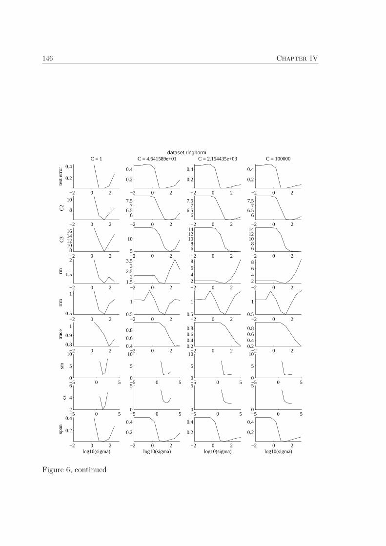
146 Chapter IV
−2 0 2
0.2
0.4
test
err
or
C = 1
−2 0 2
0.2
0.4
C = 4.641589e+01
−2 0 2
0.2
0.4
C = 2.154435e+03
−2 0 2
0.2
0.4
C = 100000
−2 0 2
8
10
C2
−2 0 2
66.5
77.5
−2 0 2
66.5
77.5
−2 0 2
66.5
77.5
−2 0 28
10121416
C3
−2 0 25
10
−2 0 2
68
101214
−2 0 2
68
101214
−2 0 2
1.5
2
rm
−2 0 21.5
22.5
33.5
−2 0 22468
−2 0 22468
−2 0 20.5
1
rrm
−2 0 20.5
1
−2 0 20.5
1
−2 0 20.5
1
−2 0 20.8
0.9
1
trac
e
−2 0 20.4
0.6
0.8
−2 0 20.20.40.60.8
−2 0 20.20.40.60.8
−5 0 50
5
10
sm
−5 0 50
5
10
−5 0 50
5
10
−5 0 50
5
10
−5 0 52
4
6
cs
−5 0 50
5
−5 0 50
5
−5 0 50
5
−2 0 2
0.2
0.4
span
log10(sigma)−2 0 2
0.2
0.4
log10(sigma)−2 0 2
0.2
0.4
log10(sigma)−2 0 2
0.2
0.4
log10(sigma)
dataset ringnorm
Figure 6, continued

A Compression Approach to Model Selection 147
−2 0 2
0.250.3
0.350.4
0.45
test
err
or
C = 1
−2 0 2
0.250.3
0.350.4
0.45
C = 4.641589e+01
−2 0 2
0.250.3
0.350.4
0.45
C = 2.154435e+03
−2 0 2
0.250.3
0.350.4
0.45
C = 100000
−2 0 2
10.5
11
C2
−2 0 2
7.6
7.8
−2 0 2
7.6
7.8
−2 0 2
7.6
7.8
−2 0 216.616.8
1717.217.417.617.8
C3
−2 0 2
10
12
14
−2 0 2
10
12
14
−2 0 2
10
12
14
−2 0 21.5
2
rm
−2 0 22.22.42.62.8
3
−2 0 2
2.53
3.5
−2 0 2
2.53
3.5
−2 0 2
0.8
1
rrm
−2 0 2
0.8
1
−2 0 2
0.8
1
−2 0 2
0.8
1
−2 0 2
1.011.021.031.041.05
trac
e
−2 0 20.4
0.6
0.8
−2 0 20.4
0.6
0.8
−2 0 20.4
0.6
0.8
−5 0 50
50
sm
−5 0 50
20
40
−5 0 50
20
40
−5 0 50
20
40
−5 0 54
5
6
cs
−5 0 52
4
6
−5 0 52
4
6
−5 0 52
4
6
−2 0 20.250.3
0.350.4
0.45
span
log10(sigma)−2 0 2
0.3
0.4
0.5
log10(sigma)−2 0 2
0.3
0.4
0.5
log10(sigma)−2 0 2
0.3
0.4
0.5
log10(sigma)
dataset splice
Figure 6, continued

148 Chapter IV
−2 0 20.050.1
0.150.2
0.25
test
err
or
C = 1
−2 0 20.050.1
0.150.2
0.25
C = 4.641589e+01
−2 0 20.050.1
0.150.2
0.25
C = 2.154435e+03
−2 0 20.050.1
0.150.2
0.25
C = 100000
−2 0 2
4
6
8
C2
−2 0 234567
−2 0 234567
−2 0 234567
−2 0 25
10
15
C3
−2 0 2
468
101214
−2 0 22468
101214
−2 0 22468
101214
−2 0 2
1
1.5
rm
−2 0 2
2
3
4
−2 0 2
51015
−2 0 2
20
40
60
−2 0 20.5
1
rrm
−2 0 2
1
1.5
2
−2 0 2
246
−2 0 2
5
10
15
−2 0 20.5
1
trac
e
−2 0 2
0.40.60.8
−2 0 2
0.40.60.8
−2 0 20.20.40.60.8
−5 0 50
20
40
sm
−5 0 50
20
40
−5 0 50
20
40
−5 0 50
20
40
−5 0 50
5
10
cs
−5 0 50
5
10
−5 0 50
5
10
−5 0 50
5
10
−2 0 2
0.1
0.2
0.3
span
log10(sigma)−2 0 2
0.1
0.2
0.3
log10(sigma)−2 0 2
0.1
0.2
0.3
log10(sigma)−2 0 2
0.1
0.2
0.3
log10(sigma)
dataset thyroid
Figure 6, continued

A Compression Approach to Model Selection 149
−2 0 2
0.25
0.3
test
err
or
C = 1
−2 0 20.2260.2280.23
0.2320.234
C = 4.641589e+01
−2 0 2
0.23
0.235C = 2.154435e+03
−2 0 20.23
0.24
0.25
C = 100000
−2 0 2
3
4
C2
−2 0 2
2.32.42.52.62.7
−2 0 2
2.25
2.3
2.35
−2 0 2
2.252.3
2.352.4
2.45
−2 0 2
9
9.5
10
C3
−2 0 28.28.48.68.8
−2 0 2
8.48.68.8
−2 0 2
8.5
9
−2 0 20.4
0.6
0.8
rm
−2 0 21
1.5
2
−2 0 2
2
4
6
−2 0 2
5101520
−2 0 20.4
0.5
0.6
rrm
−2 0 2
0.680.7
0.720.740.76
−2 0 2
0.7
0.8
0.9
−2 0 2
0.8
0.9
1
−2 0 2
0.5
1
trac
e
−2 0 2
0.5
1
−2 0 2
0.5
1
−2 0 2
0.5
1
−5 0 50
0.5
1
sm
−5 0 50
0.5
1
−5 0 516
18
20
−5 0 50
0.5
1
−5 0 50
0.5
1
cs
−5 0 50
0.5
1
−5 0 52
4
6
−5 0 50
0.5
1
−2 0 2
0.25
0.3
span
log10(sigma)−2 0 2
0.22
0.225
0.23
log10(sigma)−2 0 2
0.15
0.2
log10(sigma)−2 0 2
0.120.140.160.180.2
0.22
log10(sigma)
dataset titanic
Figure 6, continued

150 Chapter IV
−2 0 2
0.2
0.4
test
err
or
C = 1
−2 0 2
0.2
0.4
C = 4.641589e+01
−2 0 2
0.2
0.4
C = 2.154435e+03
−2 0 2
0.2
0.4
C = 100000
−2 0 26
8
10
C2
−2 0 2
4
6
−2 0 2
4
6
−2 0 2
4
6
−2 0 28
10121416
C3
−2 0 2468
101214
−2 0 2
468
101214
−2 0 2
468
101214
−2 0 21
1.5
2
rm
−2 0 2
1.5
2
−2 0 2
1.5
2
−2 0 2
1.5
2
−2 0 20.5
1
rrm
−2 0 20.5
1
−2 0 20.5
1
−2 0 20.5
1
−2 0 20.6
0.8
1
trac
e
−2 0 2
0.40.60.8
−2 0 20.20.40.60.8
−2 0 20.20.40.60.8
−5 0 50
1
2
sm
−5 0 51
1.5
2
−5 0 51
1.5
2
−5 0 51
1.5
2
−5 0 51.5
2
2.5
cs
−5 0 50
2
4
−5 0 50
2
4
−5 0 50
2
4
−2 0 2
0.2
0.4
span
log10(sigma)−2 0 2
0.2
0.4
log10(sigma)−2 0 2
0.2
0.4
log10(sigma)−2 0 2
0.2
0.4
log10(sigma)
dataset twonorm
Figure 6, continued

A Compression Approach to Model Selection 151
−2 0 2
0.2
0.3
0.4
test
err
or
C = 1
−2 0 2
0.2
0.3
0.4
C = 4.641589e+01
−2 0 2
0.2
0.3
0.4
C = 2.154435e+03
−2 0 2
0.2
0.3
0.4
C = 100000
−2 0 28.5
99.510
10.5
C2
−2 0 26.66.8
77.27.47.67.8
−2 0 26.66.8
77.27.47.67.8
−2 0 26.66.8
77.27.47.67.8
−2 0 2
14
16
C3
−2 0 28
101214
−2 0 28
101214
−2 0 28
101214
−2 0 2
1.6
1.8
rm
−2 0 22
3
4
−2 0 22
4
6
−2 0 22
4
6
−2 0 2
0.8
1
1.2
rrm
−2 0 2
0.81
1.2
−2 0 2
0.81
1.2
−2 0 2
0.81
1.2
−2 0 2
1
1.05
1.1
trac
e
−2 0 2
0.50.60.70.80.9
−2 0 20.4
0.6
0.8
−2 0 20.4
0.6
0.8
−5 0 50
10
20
sm
−5 0 50
10
20
−5 0 50
10
20
−5 0 50
10
20
−5 0 53
4
5
cs
−5 0 52
4
6
−5 0 50
5
−5 0 50
5
−2 0 2
0.2
0.3
0.4
span
log10(sigma)−2 0 2
0.2
0.3
0.4
log10(sigma)−2 0 2
0.2
0.3
0.4
log10(sigma)−2 0 2
0.2
0.3
0.4
log10(sigma)
dataset usps
Figure 6, continued

152 Chapter IV
−2 0 2
0.150.2
0.250.3
test
err
or
C = 1
−2 0 2
0.2
0.3
C = 4.641589e+01
−2 0 2
0.2
0.3
C = 2.154435e+03
−2 0 2
0.2
0.3
C = 100000
−2 0 2
7
8
9
C2
−2 0 2
567
−2 0 26
7
−2 0 2
6.5
7
7.5
−2 0 210
15
C3
−2 0 268
101214
−2 0 25
10
−2 0 2
68
101214
−2 0 2
1.2
1.4
1.6
rm
−2 0 2
22.5
3
−2 0 22
4
6
8
−2 0 22468
−2 0 20.6
0.8
1
rrm
−2 0 20.60.8
11.2
−2 0 2
11.5
2
−2 0 2
11.5
2
−2 0 20.9
1
1.1
trac
e
−2 0 20.4
0.6
0.8
−2 0 2
0.40.60.8
−2 0 2
0.40.60.8
−5 0 51
1.5
2
sm
−5 0 51.5
2
2.5
−5 0 51
2
3
−5 0 51
2
3
−5 0 52
2.2
2.4
cs
−5 0 51
1.5
2
−5 0 51
1.5
2
−5 0 51
1.5
2
−2 0 20.150.2
0.250.3
span
log10(sigma)−2 0 2
0.2
0.3
log10(sigma)−2 0 2
0.2
0.3
log10(sigma)−2 0 2
0.2
0.3
log10(sigma)
dataset waveform
Figure 6, continued

A Compression Approach to Model Selection 153
−2 0 2
0.1
0.2
0.3
test
err
or
C = 1
−2 0 2
0.1
0.2
0.3
C = 4.641589e+01
−2 0 2
0.1
0.2
0.3
C = 2.154435e+03
−2 0 2
0.1
0.2
0.3
C = 100000
−2 0 2
468
C2
−2 0 22
4
6
−2 0 2
4
6
−2 0 2
4
6
−2 0 2
5
10
15
C3
−2 0 22468
1012
−2 0 22468
1012
−2 0 22468
1012
−2 0 20.8
11.21.41.6
rm
−2 0 2
1.5
2
2.5
−2 0 2
2
4
−2 0 2
2
4
−2 0 20.5
1
rrm
−2 0 20.5
1
−2 0 20.5
1
1.5
−2 0 20.5
1
1.5
−2 0 20.5
1
trac
e
−2 0 20.4
0.6
0.8
−2 0 20.4
0.6
0.8
−2 0 20.4
0.6
0.8
−5 0 50
5
10
sm
−5 0 50
5
10
−5 0 50
5
10
−5 0 50
5
10
−5 0 50
2
4
cs
−5 0 50
2
4
−5 0 50
2
4
−5 0 50
2
4
−2 0 2
0.2
0.4
span
log10(sigma)−2 0 2
0.2
0.4
log10(sigma)−2 0 2
0.2
0.4
log10(sigma)−2 0 2
0.2
0.4
log10(sigma)
dataset wisconsin
Figure 6, continued


Notation
General:
X input spaceY output spacexi or Xi training patternsyi or Yi training labelsn number of training points1 constant-1 function (or vector)0 constant-0 function (or vector)1A characteristic function of the set A(C(X ), ‖ · ‖∞) space of continuous functions on X with infinity
normP probability distribution on the data spacePn empirical distribution` loss functionR true risk (p. 70)Remp empirical risk (p. 70)Rreg regularized risk (p. 71)Rn Rademacher complexity (p. 71)
Rn maximum discrepancy (p. 71)
Rn empirical Rademacher complexity (p. 71)N(F , ε, d) ε-covering numbers of the space F with respect to
metric d (p. 94)
Chapter II:
k similarity functionKn similarity or kernel matrix of size n× n (p. 22)Dn degree matrix (p. 22)Ln unnormalized graph Laplacian (p. 22)L′n symmetrically normalized graph Laplacian (p. 22)L′′n row-sum normalized graph Laplacian (p. 22)
156 Notation
H ′n symmetrically normalized similarity matrix (p.
23)H ′
n row-sum normalized similarity matrix (p. 23)d and dn degree functions, true and empirical (p. 35)h and hn symmetrically normalized similarity functions,
true and empirical (p. 36)g and gn row-sum normalized similarity functions, true and
empirical (p. 37)
Snp→ S pointwise convergence (p. 32)
Snc→ S compact convergence (p. 32)
Sncc→ S collectively compact convergence (p. 32)
Sn‖·‖→ S convergence in operator norm (p. 32)
Sn+−→ S convergence up to a change of sign (p. 29)
Chapter III:
(X , d) metric space(X0, d0) extended metric space (p. 81)diam diameter of a metric space (p. 80)L(f) Lipschitz constant of function f (p. 79)(Lip(X ), ‖ · ‖L) Lipschitz function space (p. 80)(Lip0(X0), L(·)) another Lipschitz function space (p. 80)(AE(X ), ‖ · ‖AE) Arens-Eells space (p. 81)
Chapter IV:
log logarithm to base 2R radius of the smallest ball sphere the training dataρ margind dimension of the feature spaceC1 − C5 compression coefficients
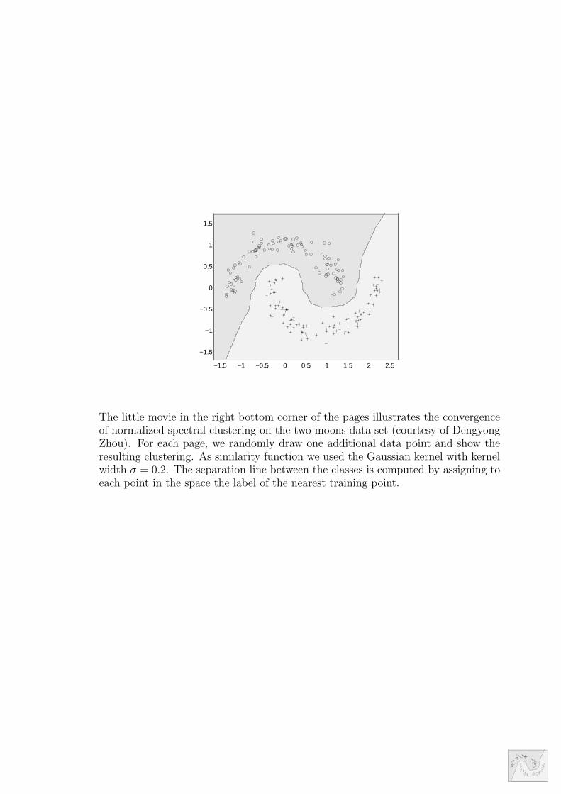
−1.5 −1 −0.5 0 0.5 1 1.5 2 2.5
−1.5
−1
−0.5
0
0.5
1
1.5
The little movie in the right bottom corner of the pages illustrates the convergenceof normalized spectral clustering on the two moons data set (courtesy of DengyongZhou). For each page, we randomly draw one additional data point and show theresulting clustering. As similarity function we used the Gaussian kernel with kernelwidth σ = 0.2. The separation line between the classes is computed by assigning toeach point in the space the label of the nearest training point.


Bibliography
P. Anselone. Collectively compact operator approximation theory. Prentice-Hall,Englewood Cliffs, New Jersey, 1971.
M. Anthony. Uniform Glivenko-Cantelli theorems and concentration of measure inthe mathematical modelling of learning. CDAM Research Report LSE-CDAM-2002-07, 2002.
R. Arens and J. Eells. On embedding uniform and topological spaces. Pacific J.Math., 6:397–403, 1956.
C. Baker. The numerical treatment of integral equations. Oxford University Press,1977.
S. Barnard, A. Pothen, and H. Simon. A spectral algorithm for envelope reduction ofsparse matrices. Numerical Linear Algebra with Applications, 2(4):317–334, 1995.
A. Barron, J. Rissanen, and B. Yu. The minimum description length principle incoding and modeling. IEEE Trans. Inform. Theory, 44(6):2743 – 2760, 1998.
P. Bartlett and S. Mendelson. Rademacher and Gaussian complexities: Risk boundsand structural results. In D. Helmbold and B. Williamson, editors, Proceedingsof the 14th annual conference on Computational Learning Theory, pages 273–288,2001.
P. Bartlett and S. Mendelson. Rademacher and Gaussian complexities: Risk boundsand structural results. JMLR, 3:463–482, 2002.
P. L. Bartlett and J. Shawe-Taylor. Generalization performance of support vectormachines and other pattern classifiers. In B. Scholkopf, C. J. C. Burges, and A. J.Smola, editors, Advances in Kernel Methods — Support Vector Learning, pages43–54. MIT Press, Cambridge, MA, 1999.
M. Belkin. Problems of Learning on Manifolds. PhD thesis, University of Chicago,2003.
M. Belkin and P. Niyogi. Laplacian eigenmaps for dimensionality reduction anddata representation. Neural Computation, 15(6):1373–1396, June 2003a.

160 Bibliography
M. Belkin and P. Niyogi. Using manifold structure for partially labeled classification.In S. Thrun S. Becker and K. Obermayer, editors, Advances in Neural InformationProcessing Systems 15, Cambridge, MA, 2003b. MIT Press.
Y. Bengio, P. Vincent, J.-F. Paiement, O. Delalleau, M. Ouimet, and N. Le Roux.Spectral clustering and kernel PCA are learning eigenfunctions. Technical ReportTR 1239, University of Montreal, 2003.
K. Bennett and E. Bredensteiner. Duality and geometry in SVM classifiers. InP. Langley, editor, Proceedings of the Seventeenth International Conference onMachine Learning, pages 57–64. Morgan Kaufmann, San Francisco, 2000.
R. Bhatia. Matrix Analysis. Springer, New York, 1997.
T. De Bie, M. Momma, and N. Cristianini. Efficiently learning the metric with side-information. In Algorithmic Learning Theory, 14th International Conference, ALT2003, Sapporo, Japan, October 2003, Proceedings, volume 2842 of Lecture Notesin Artificial Intelligence, pages 175–189. Springer, 2003.
M. Birman and M. Solomjak. Spectral theory of self-adjoint operators in Hilbertspace. Reidel Publishing Company, Dordrecht, 1987.
A. Blum and J. Langford. PAC-MDL bounds. In B. Scholkopf and M.K. Warmuth,editors, Learning Theory and Kernel Machines, pages 344–357. 16th Annual Con-ference on Learning Theory, Springer, Berlin, 2003.
M. Bolla. Relations between spectral and classification properties of multigraphs.Technical Report 91-27, DIMACS Technical Report, 1991.
L. Bottou and Y. Bengio. Convergence properties of the k-means algorithm. InD. Touretzky, M. Mozer, and M. Hasselmo, editors, Advances in Neural Informa-tion Processing Systems 8. MIT Press, Denver, 1995.
O. Bousquet. Concentration Inequalities and Empirical Processes Theory Applied tothe Analysis of Learning Algorithms. PhD thesis, Ecole Polytechnique, 2002.
O. Bousquet, O. Chapelle, and M. Hein. Measure based regularization. In S. Thrun,L. Saul, and B. Scholkopf, editors, Advances in Neural Information ProcessingSystems 16. MIT Press, Cambridge, MA, 2004.
O. Bousquet and D. Herrmann. On the complexity of learning the kernel matrix. InS. Thrun S. Becker and K. Obermayer, editors, Advances in Neural InformationProcessing Systems, 15, Cambridge, MA, 2003. MIT Press.
Pierre Bremaud. Markov chains: Gibbs fields, Monte Carlo simulation, and queues,volume 31 of Texts in Applied Mathematics. Springer-Verlag, New York, 1999.
O. Chapelle and V. Vapnik. Model selection for support vector machines. In S. A.Solla, T. K. Leen, and K.-R. Muller, editors, Advances in Neural InformationProcessing Systems 12. MIT Press, Cambridge, MA, 2000.

Bibliography 161
F. Chatelin. Spectral Approximation of Linear Operators. Academic Press, NewYork, 1983.
F. Chung. Spectral graph theory, volume 92 of CBMS Regional Conference Series inMathematics. Published for the Conference Board of the Mathematical Sciences,Washington, DC, 1997.
J. Conway. A Course in Functional Analysis. Springer, New York, 1985.
T. M. Cover and J. A. Thomas. Elements of Information Theory. Wiley, New York,1991.
T. Cox and A. Cox. Multidimensional Scaling. Chapman & Hall, London, 2ndedition, 2001.
N. Cristianini and J. Shawe-Taylor. An Introduction to Support Vector Machinesand other kernel-based learning methods. Cambridge University Press, Cambridge,UK, 2000.
A. Cuevas, M. Febrero, and R. Fraiman. Cluster analysis: a further approach basedon density estimation. Computational Statistics and Data Analysis, 36:441–459,2001.
L. Devroye, L. Gyorfi, and G. Lugosi. A Probabilistic Theory of Pattern Recognition.Springer, New York, 1996.
L. Devroye and G. Lugosi. Combinatorial Methods in Density Estimation. Springer,New York, 2001.
V. Dobric and J. Yukich. Asymptotics for transportation costs in high dimensions.J. Theor. Probab., 8(1):97–118, 1995.
W. E. Donath and A. J. Hoffman. Lower bounds for the partitioning of graphs.IBM J. Res. Develop., 17:420–425, 1973.
R. M. Dudley. Universal Donsker classes and metric entropy. Ann. Probab., 15(4):1306–1326, 1987.
N. Dunford and J. Schwartz. Linear Operators, Part I. Interscience Publishers, NewYork, 1957.
M. Fiedler. Algebraic connectivity of graphs. Czechoslovak Math. J., 23:298–305,1973.
S. Floyd and Manfred K. Warmuth. Sample compression, learnability, and theVapnik-Chervonenkis dimension. Machine Learning, 21(3):269–304, 1995.
L. Goldfarb. A new approach to pattern recognition. In L. Kanal and A. Rosenfeld,editors, Progress in Pattern Recognition, volume 2, pages 241–402. Elsevier, North-Holland, 1985.

162 Bibliography
J. Gower. Measures of similarity, dissimilarity, and distance. In S. Kotz and N. John-son, editors, Encyclopedia of Statistical Sciences, volume 5, pages 397–405. Wiley,New York, 1985.
J. Gower. Metric and Euclidean properties of dissimilarity coefficients. Journal ofclassification, 3:5–48, 1986.
T. Graepel, R. Herbrich, P. Bollmann-Sdorra, and K. Obermayer. Classification onpairwise proximity data. In M. S. Kearns, S. A. Solla, and D. A. Cohn, editors,Advances in Neural Information Processing Systems, volume 11, pages 438–444.MIT Press, Cambridge, MA, 1999a.
T. Graepel, R. Herbrich, B. Scholkopf, A. Smola, P. Bartlett, K. Muller, K. Ober-mayer, and R. Williamson. Classification of proximity data with LP machines. InProceedings of the Ninth International Conference on Artificial Neural Networks,pages 304–309, 1999b.
S. Guattery and G. L. Miller. On the quality of spectral separators. SIAM Journalof Matrix Anal. Appl., 19(3), 1998.
L. Hagen and A.B. Kahng. New spectral methods for ratio cut partitioning andclustering. IEEE Trans. Computer-Aided Design, 11(9):1074–1085, 1992.
M. Hansen and B. Yu. Model selection and the principle of minimum descriptionlength. Journal of the American Statistical Association, 96(454):746–774, 2001.
J. Hartigan. Clustering algorithms. Wiley, New York, 1975.
J. Hartigan. Consistency of single linkage for high-density clusters. JASA, 76(374):388–394, 1981.
J. Hartigan. Statistical theory in clustering. Journal of classification, 2:63–76, 1985.
M. Hein and O. Bousquet. Maximal margin classification for metric spaces. InM. Warmuth B. Scholkopf, editor, Proceedings of the 16. Annual Conference onComputational Learning Theory, pages 72–86. Springer Verlag, Heidelberg, 2003.
B. Hendrickson and R. Leland. An improved spectral graph partitioning algorithmfor mapping parallel computations. SIAM J. on Scientific Computing, 16:452–469,1995.
R. Herbrich, T. Graepel, and J. Shawe-Taylor. Sparsity vs. large margins for linearclassifiers. In N. Cesa-Bianchi and S. Goldman, editors, Proceedings of the Thir-teenth Annual Conference on Computational Learning Theory, pages 304–308.Morgan Kaufmann, San Francisco, 2000.
D. Higham and M. Kibble. A unified view of spectral clustering. MathematicsResearch Report 2, University of Strathclyde, 2004.

Bibliography 163
D. Hochbaum and D. Shmoys. A best possible heuristic for the k-center problem.Mathematics of Operations Research, 10(2):180–184, 1985.
N. Jardine and R. Sibson. Mathematical taxonomy. Wiley, London, 1971.
R. Kannan, S. Vempala, and A. Vetta. On clusterings - good, bad and spectral.Technical report, Computer Science Department, Yale University, 2000.
T. Kato. Perturbation theory for linear operators. Springer, Berlin, 1966.
J. Kleinberg. An impossibility theorem for clustering. In S. Thrun S. Becker andK. Obermayer, editors, Advances in Neural Information Processing Systems 15,pages 446–453. MIT Press, Cambridge, MA, 2003.
A. N. Kolmogorov and V. M. Tihomirov. ε-entropy and ε-capacity of sets in func-tional space. Amer. Math. Soc. Transl. (2), 17:277–364, 1961.
V. Koltchinskii. Asymptotics of spectral projections of some random matrices ap-proximating integral operators. Progress in Probabilty, 43, 1998.
V. Koltchinskii and E. Gine. Random matrix approximation of spectra of integraloperators. Bernoulli, 6(1):113 – 167, 2000.
G. Lanckriet, N. Cristianini, P. Bartlett, L. El Ghaoui, and M. Jordan. Learningthe kernel matrix with semidefinite programming. JMLR, 5:27–72, 2004.
J. Lember. On minimizing sequences for k-centres. Journal of Approximation The-ory, 120:20–35, 2003.
G. Lugosi and A. Nobel. Consistency of data-driven histogram methods for densityestimation and classification. Ann. Statist., 24(2):687–706, 1996.
K. Mardia, J. Kent, and J. Bibby. Multivariate Analysis. Academic Press, London,1979.
D. McAllester. Some PAC–Bayesian theorems. Machine Learning, 37(3):355–363,1999.
R. Megginson. An introduction to Banach space theory. Springer, New York, 1998.
M. Meila and J. Shi. A random walks view of spectral segmentation. In 8th Inter-national Workshop on Artificial Intelligence and Statistics, 2001.
S. Mendelson and R. Vershynin. Entropy and the combinatorial dimension. Inven-tiones Mathematicae, 152(1):37–55, 2003.
B. Mohar. The Laplacian spectrum of graphs. In Graph theory, combinatorics, andapplications. Vol. 2 (Kalamazoo, MI, 1988), Wiley-Intersci. Publ., pages 871–898.Wiley, New York, 1991.

164 Bibliography
A. Ng, M. Jordan, and Y. Weiss. On spectral clustering: Analysis and an algorithm.In T. Dietterich, S. Becker, and Z. Ghahramani, editors, Advances in NeuralInformation Processing Systems 14. MIT Press, 2001.
P. Niyogi and N. K. Karmarkar. An approach to data reduction and clustering withtheoretical guarantees. In P. Langley, editor, Proceedings of the Seventeenth In-ternational Conference on Machine Learning. Morgan Kaufmann, San Francisco,2000.
M. Opper and O. Winther. Gaussian processes and SVM: mean field and leave-one-out. In A. J. Smola, P. L. Bartlett, B. Scholkopf, and D. Schuurmans, editors,Advances in Large Margin Classifiers, pages 311–326. MIT Press, Cambridge, MA,2000.
E. Pekalska, P. Paclık, and R. Duin. A generalized kernel approach to dissimilar-ity based classification. Journal of Machine Learning Research, 2:175–211, 2001.Special Issue ”New Perspectives on Kernel Based Learning Methods”.
V. Pestov. Free Banach spaces and representations of topological groups. Funct.Anal. Appl, 20:70–72, 1986.
D. Pollard. Strong consistency of k-means clustering. Annals of Statistics, 9(1):135–140, 1981.
J. Puzicha, T. Hofmann, and J. Buhmann. A theory of proximity based clustering:Structure detection by optimization. Pattern Recognition, 33(4):617–634, 2000.
G. Ratsch, T. Onoda, and K.-R. Muller. Soft margins for AdaBoost. MachineLearning, 42(3):287–320, March 2001.
S. Roweis and L. Saul. Nonlinear dimensionality reduction by locally linear embed-ding. Science, 290:2323–2326, 2000.
W. Rudin. Functional Analysis. McGraw-Hill Inc., Singapore, 2nd edition, 1991.
I. Schoenberg. Metric spaces and positive definite functions. TAMS, 44:522–536,1938.
B. Scholkopf. The kernel trick for distances. In T. G. Dietterich T. K. Leen andV. Tresp, editors, Advances in Neural Information Processing Systems 13. MITPress, Cambridge, MA, 2001.
B. Scholkopf and A. Smola. Learning with Kernels. MIT Press, Cambridge, MA,2002.
J. Shawe-Taylor, C. Williams, N. Cristianini, and J. Kandola. On the eigenspec-trum of the Gram matrix and its relationship to the operator eigenspectrum. InN. Cesa-Bianchi, M. Numao, and R. Reischuk, editors, Proceedings of the 13thInternational Conference on Algorithmic Learning Theory. Springer, Heidelberg,2002.
Bibliography 165
J. Shi and J. Malik. Normalized cuts and image segmentation. IEEE Transactionson Pattern Analysis and Machine Intelligence, 22(8):888–905, 2000.
A. J. Smola, B. Scholkopf, and K.-R. Muller. The connection between regularizationoperators and support vector kernels. Neural Networks, 11:637–649, 1998.
D. Spielman and S. Teng. Spectral partitioning works: planar graphs and finiteelement meshes. In 37th Annual Symposium on Foundations of Computer Science(Burlington, VT, 1996), pages 96–105. IEEE Comput. Soc. Press, Los Alamitos,CA, 1996.
J. M. Steele. Probability theory and combinatorial optimization, volume 69 of CBMS-NSF Regional Conference Series in Applied Mathematics. Society for Industrialand Applied Mathematics (SIAM), Philadelphia, PA, 1997.
M. Talagrand. The Ajtai-Komlos-Tusnady matching theorem for general measures.In Probability in Banach spaces, 8 (Brunswick, ME, 1991), volume 30 of Progr.Probab., pages 39–54. Birkhauser Boston, Boston, MA, 1992.
A. Taylor. Introduction to Functional Analysis. Wiley, New York, 1958.
J. Tenenbaum, V. de Silva, and J. Langford. A global geometric framework fornonlinear dimensionality reduction. Science, 290:2319–2323, 2000.
A. W. van der Vaart and J. A. Wellner. Weak Convergence and Empirical Processes.Springer, New York, 1996.
R. Van Driessche and D. Roose. An improved spectral bisection algorithm and itsapplication to dynamic load balancing. Parallel Comput., 21(1), 1995.
V. Vapnik. The Nature of Statistical Learning Theory. Springer Verlag, New York,1995.
V. Vapnik. Statistical Learning Theory. Wiley, New York, 1998.
V. Vapnik and O. Chapelle. Bounds on error expectation for support vector ma-chines. Neural Computation, 12(9):2013–2036, 2000.
R. Veltkamp and M. Hagedoorn. Shape similarity measures, properties and con-structions. In Advances in Visual Information Systems, Proceedings of the 4thInternational Conference, pages 467–476. Springer, 2000.
D. Verma and M. Meila. A comparison of spectral clustering algorithms. TechnicalReport UW CSE Technical report 03-05-01, University of Washington, 2003.
U. von Luxburg and O. Bousquet. Distance-based classification with Lipschitz func-tions. In B. Scholkopf and M.K. Warmuth, editors, Proceedings of the 16th AnnualConference on Learning Theory (COLT), pages 314–328. Springer, 2003. This ar-ticle won the prize for the best student paper.

166 Bibliography
U. von Luxburg and O. Bousquet. Distance-based classification with Lipschitz func-tions. Journal for Machine Learning Research, 5:669–695, 2004.
U. von Luxburg, O. Bousquet, and M. Belkin. Limits of spectral clustering. InAdvances in Neural Information Processing Systems 18, 2004a. to appear.
U. von Luxburg, O. Bousquet, and M. Belkin. On the convergence of spectralclustering on random samples: the normalized case. In J. Shawe-Taylor andY. Singer, editors, Proceedings of the 17th Annual Conference on Learning Theory(COLT), pages 457–471. Springer, 2004b.
U. von Luxburg, O. Bousquet, and B. Scholkopf. A compression approach to supportvector model selection. Journal for Machine Learning Research, 5:293–323, 2004c.
S. Watson. The classification of metrics and multivariate statistical analysis. Topol-ogy and its Applications, 99:237–261, 1999.
N. Weaver. Lipschitz algebras. World Scientific, Singapore, 1999.
J. Weidmann. Linear Operators in Hilbert spaces. Springer, New York, 1980.
Y. Weiss. Segmentation using eigenvectors: A unifying view. In Proceedings of theInternational Conference on Computer Vision, pages 975–982, 1999.
C. K. I. Williams and M. Seeger. The effect of the input density distribution onkernel-based classifiers. In P. Langley, editor, Proceedings of the 17th Interna-tional Conference on Machine Learning, pages 1159–1166. Morgan Kaufmann,San Francisco, 2000.
W. Wright. A formalization of cluster analysis. Pattern Recognition, 5:273–282,1973.
E. Xing, A. Ng, M. Jordan, and S. Russell. Distance metric learning with applicationto clustering with side-information. In S. Thrun S. Becker and K. Obermayer,editors, Advances in Neural Information Processing Systems 15, pages 505–512.MIT Press, Cambridge, MA, 2003.
S. Zhong and J. Ghosh. A unified framework for model-based clustering. JMLR, 4:1001–1037, 2003.
D. Zhou and B. Scholkopf. Learning from labeled and unlabeled data using randomwalks. Technical report, Max Planck Institute for Biological Cybernetics, March2004.
D. Zhou, B. Xiao, H. Zhou, and R. Dai. Global geometry of SVM classifiers. Techni-cal Report 30-5-02, Institute of Automation, Chinese Academy of Sciences, 2002.
X. Zhu, Z. Ghahramani, and J. Lafferty. Semi-supervised learning using Gaussianfields and harmonic functions. In T. Fawcett and N.Mishra, editors, Proceedingsof the 20th International Conference of Machine Learning. AAAI Press, 2003.