Statistical Mechanics of On-line learning

Michael Biehl1, Nestor Caticha2, and Peter Riegler3

1 University of Groningen, Inst. of Mathematics and Computing Science,P.O. Box 407, 9700 AK Groningen, The Netherlands,

2 Instituto de Fisica, Universidade de Sao Paulo,CP66318, CEP 05315-970, Sao Paulo, SP Brazil,

3 Fachhochschule Braunschweig/Wolfenbuttel, Fachbereich Informatik,Salzdahlumer Str. 46/48, 38302 Wolfenbuttel, Germany

Abstract. We introduce and discuss the application of statistical physicsconcepts in the context of on-line machine learning processes. The con-sideration of typical properties of very large systems allows to perfom av-erages over the randomness contained in the sequence of training data.It yields an exact mathematical description of the training dynamicsin model scenarios. We present the basic concepts and results of theapproach in terms of several examples, including the learning of linearseparable rules, the training of multilayer neural networks, and LearningVector Quantization.

1 Introduction

The perception that Statistical Mechanics is an inference theory has openedthe possibility of applying its methods to several areas outside the traditionalrealms of Physics. This explains the interest of part of the Statistical Mechanicscommunity during the last decades in machine learning and optimization and theapplication of several techniques of Statistical Mechanics of disordered systemsin areas of Computer Science.

As an inference theory Statistical Mechanics is a Bayesian theory. Bayesianmethods typically demand extended computational resources which probablyexplains why methods that were used by Laplace, were almost forgotten in thefollowing century. The current availability of ubiquitous and now seemingly pow-erful computational resources has promoted the diffusion of these methods instatistics. For example, posterior averages can now be rapidly estimated by us-ing efficient Markov Chain Monte Carlo methods, which started to be developedto attack problems in Statistical Mechanics in the middle of last century. Ofcourse the drive to develop such techniques (starting with [1]) is due to the totalimpossibility of introducing classical statistics methods to study thermodynamicproblems. Several other techniques Statistical Mechanics have also found theirway into statistics. In this paper we review some applications of Statistical Me-chanics to artificial machine learning.

Learning is the change induced by the arrival of information. We are inter-ested in learning from examples. Different scenarios arise if examples are con-sidered in batches or just one at a time. This last case is the on-line learning

II

scenario and the aim of this contribution is to present the characterization of on-line learning using methods of Statistical Mechanics. We will consider in section2 simple linearly separable classification problems , just to introduce the idea.The dynamics of learning is described by a set of stochastic difference equationswhich show the evolution, as information arrives, of quantities that characterizethe problem and in Statistical Mechanics are called order parameters. Lookingat the limit of large dimensions and scaling the number of examples in a correctmanner, the difference equations simplify into deterministic ordinary differen-tial equations. Numerical solutions of the ODE give then, for the specific modelof the available information such as the distribution of examples, the learningcurves.

While this large dimension limit may seem artificial, it must be stressed thatit is most sensible in the context of thermostatistics, where Statistical Mechanicsis applied to obtain thermodynamic properties of physical systems. There the di-mension, which is the number of degrees of freedom, is of the order of Avogadro’snumber ( ≈ 1023). Simulations however have to be carried for much smaller sys-tems, and this prompted the study of finite size corrections of expectations ofexperimentally relevant quantities, which depend on several factors, but typi-cally go to zero algebraically with the dimension. If the interest lies in intensivequantities such as temperature, pressure or chemical potential then correctionsare negligible. If one is interested on extensive quantities, such as energy, entropyor magnetization, one has to deal with their densities, such as energy per degreeof freedom. Again the errors due to the infinite size limit are negligible. In thislimit, central limit theorems apply , resulting in deterministic predictions andthe theory is in the realm of thermodynamics. Thus this limit is known as thethermodynamic limit (TL). For inference problems we can use the type of theoryto control finite size effects in the reverse order. We can calculate for the easierdeterministic infinite limit and control the error made by taking the limit. Wemention this and give references, but will not deal with this problem except bynoticing that it is theoretically understood and that simulations of stylized mod-els, necessarily done in finite dimensions, agree well with the theoretical resultsin the TL. The reader might consider that the thermodynamic limit is equivalentto the limit of infinite sequences in Shannon’s channel theorem.

Statistical Mechanics (see e.g. [2,3]) had its origins in the second half of theXIX century, in an attempt, mainly due to Maxwell, Boltzmann and Gibbs todeduce from the microscopic dynamical properties of atoms and molecules, themacroscopic thermodynamic laws. Its success in building a unified theoreticalframework which applied to large quantities of experimental setups was one ofthe great successes of Physics in the XIX century. A measure of its successcan be seen from its role in the discovery of Quantum Mechanics. Late in theXIX century, when its application to a problem where the microscopic lawsinvolved electromagnetism, i.e the problem of Black Body radiation, showedirreconcilable results with experiment, Max Planck showed that the problem laidwith the classical laws of electromagnetism and not with Statistical Mechanics.This started the revolution that led to Quantum Mechanics.

III

This work is organized as follows. We introduce the method in section 2the main ideas in a simple model. Section 3 will look into the extension of on-line methods to the richer case of two-layered networks which include universalapproximators. In section 4 we present the latest advances in the area which dealwith characterizing theoretically clustering methods such as Learning VectorQuantization (LVQ).

This paper is far from giving a complete overview of this successful approachto machine learning. Our intention is to illustrate the basic concepts in terms ofselected examples, mainly from our own work. Also references are by no meanscomplete and serve merely as a starting point for the interested reader.

2 On-line learning in Classifiers: Linearly separable case

We consider a supervised classification problem, where vectors ξ ∈ RN have tobe classified into one of two classes which we label by +1 or −1 respectively.These vectors are drawn independently from a probability distribution Po(ξ).The available information is in the form of example pairs of vector-label: (ξν , σν),ν = 1, 2...µ. The scenario of on-line learning is defined by the fact that we takeinto account one pair at a time, which permits to identify ν and µ as timeindexes. We also restrict our attention to the simple case where examples areused once to induce some change in our machine and then are discarded. Whilethis seems quite inefficient since recycling examples to extract more informationcan indeed be useful, it permits to develop a simple theory due to the assumptionof independence of the examples. The recycling of examples can also be treated([4]) but it needs a repertoire of techniques that is beyond the scope of thisreview. For many simple cases this will be seen to be quite efficient.

As a measure of the efficiency of the learning algorithm we will concentrateon the generalization error, which is the probability of making a classificationerror on a new, statistically independent example ξµ+1. If any generalizationis at all possible, of course there must be an underlying rule to generate theexample labels, which is either deterministic

σB = fB(ξ) (1)

or described by the conditional probability P (σB|fB(ξ)) depending on a transferfunction fB parameterized by a set of K unknown parameters B. At this pointwe take B to be fixed in time, a constraint that can be relaxed and still bestudied within the theory, see [5,6,7,8].

Learning is the compression of information from the set of µ example pairsinto a set of M weights Jµ ∈ RM and our machine classifies according to

σJ = gJ(ξ) (2)

The generalization error is

IV

eG(µ) =

∫

dPo(ξ)

∫ µ∏

ν=1

dPo(ξν)∑

σν=±1

P (σBν |fB(ξν))Θ(−σJµσB(ξ))

= 〈Θ(−σJµ(ξ)σB(ξ))〉{σν ,ξν}ν=1,µ,σ,ξ, (3)

where the step function Θ(x) = 1 for x > 0 and zero otherwise. As this standsit is impossible to obtain results other than of a general nature. To obtain sharpresults we have to specify a model.

The transfer functions fB and gJ specify the architectures of the rule and ofthe classifier, while P (σµ|fB(ξµ)) models possible noise in the specification ofthe supervision label. The simplest case that can be studied is where both fB

and gJ are linearly separable classifiers of the same dimension: K = M = N ,

σJ = sign(J .ξ), σB = sign(B.ξ) (4)

As simple and artificial as it may be, the study of this special case serves severalpurposes and is a stepping stone into more realistic scenarios.

An interesting feature of Statistical Mechanics lies in that it points out whatare the relevant order parameters in a problem. In physics, this turns out to beinformation about what are the objects of experimental interest.

Without any loss we can take all vectors ξ and B to be normalized as ξ·ξ = Nand B ·B = 1. For J however, which is a dynamical quantity that evolves underthe learning algorithm still to be specified we let it free and call J · J = Q.Define the fields

h = J · ξ, b = B · ξ (5)

To advance further we choose a model for the distribution of examples Po(ξ)and the natural starting point is to choose a uniform distribution over the N -dimensional sphere. Different choices to model specific situation are of coursepossible. Under these assumptions, since the scalar products of (4) are sumsof random variables, for large N , h and b are correlated Gaussian variables,completely characterized by

〈h〉 = 〈b〉 = 0,

〈h2〉 = Q, 〈b2〉 = 1,

〈hb〉 = J · B = R. (6)

It is useful to introduce the overlap ρ = R/√

Q between the rule and machineparameter vectors. The joint distribution is given by

P (h, b) =1

2π√

(1 − ρ2)e− 1

2(1−ρ2)(h2−2ρhb+b2)

. (7)

The correlation is the overlap ρ, which is related to the angle φ between J andB: φ = cos−1 ρ, it follows that |ρ| ≤ 1. It is geometrically intuitive and also easy

V

to prove that the probability of making an error on an independent example,the generalization error, is φ/2π:

eG =1

2πcos−1 ρ (8)

The strategy now is to introduce a learning algorithm, i.e to define the changethat the inclusion of a new example causes in J , calculate the change in theoverlap ρ and then obtain the learning curve for the generalization error. Wewill consider learning algorithms of the form

Jµ+1 = Jµ +F

Nξµ+1, (9)

where F , called the modulation function of vector ξµ+1, should depend on thesupervised information, the label σB

µ+1. It may very well depend on some addi-tional information carried by hyperparameters or on ξ itself. It is F that definesthe learning algorithm. We consider the case where F is a scalar function, butit could differ for different components of ξ. Projecting (9) into B and into J

we obtain respectively

Rµ+1 = Rµ +F

Nbµ (10)

Qµ+1 = Qµ + 2F

Nhµ +

F 2

N. (11)

which describe the learning dynamics. We can also write an equivalent equationfor the overlap ρ which is valid for large N and ξ on the hypersphere and

ρµ+1 =Jµ+1.B√

Qµ+1

=

= ρµ

(

1 − 1

N

F√

Qµ

hµ+1 −1

2N(

F√

Qµ

)2

)

+1

N

F√

Qµ

bµ+1 (12)

∆ρµ+1 =1

N

F√

Qµ

(bµ+1 − ρµhµ+1) −1

2N

ρµF 2

Qµ(13)

Since at each time step µ a random vector is drawn from the distribution Po

equations (12) and (13) are stochastic difference equations. We now take thethermodynamic limit N → ∞ and average over the test example ξ. Note thateach example induces a change of the order parameters of order 1/N . Hence,one expects the need of order N many examples to create a change of order 1.This prompts the introduction of α = limN→∞ µ/N which by measuring thenumber of examples measures time. The behavior of ρ and ∆ρ

∆α are very differentin the limit. It can be shown (see [9]) that order parameters such as ρ, R, Q self-average. Their fluctuations tend to zero in this limit, see Fig. 3 for an example.On the other hand ∆ρ

∆α has fluctuations of order one and we look at its averageover the test vector:

dρ

dα= 〈∆ρ

∆α〉h,b,ξ. (14)

VI

the pairs (Q, ∆Q/∆α) and (R, ∆R/∆α) behave in a similar way. We averageover the fields h, b and over the labels σ, using P (σ|b) .This leads to the coupledsystem of ordinary differential equations, which for a particular form of F wereintroduced in [10].

dR

dα=∑

σ

∫

dhdbP (h, b)P (σ|b) [Fb] = 〈Fb〉 (15)

dQ

dα=∑

σ

∫

dhdbP (h, b)P (σ|b)[

2Fh + F 2]

= 〈2Fh + F 2〉, (16)

where the angular brackets stand for the average over the fields and label. Sincethe generalization error is directly related to ρ it will be useful to look at theequivalent set of equations for ρ and the length of the weight vector

√Q:

dρ

dα=∑

σ

∫

dhdbP (h, b)P (σ|b)[

F√Q

(b − ρh) − ρF 2

2Q

]

(17)

d√

Q

dα=∑

σ

∫

dhdbP (h, b)P (σ|b)[

Fh +1

2

F 2

√Q

]

(18)

We took the average with respect to the two fields h and b as if they stood onsymmetrical grounds, but they don’t. It is reasonable to assume knowledge of hand σ but not of b. Making this explicit

dρ

dα=∑

σ

∫

dhP (h)P (σ)

[

F√Q〈b − ρh〉b|σh − ρF 2

2Q

]

(19)

d√

Q

dα=∑

σ

∫

dhP (h)P (σ)

[

Fh +1

2

F 2

√Q

]

(20)

call

F ∗ =

√Q

ρ〈b − ρh〉b|σh (21)

where the average is over unavailable quantities. Equation 19 can then be writtenas

dρ

dα=

ρ

Q

∑

σ

∫

dhP (h)P (σ)

[

FF ∗ − 1

2F 2

]

(22)

This notation makes it natural to ask for an interpretation of the meaning ofF ∗. The differential equations above describe the dynamics for any modulationfunction. We can ask ([11]) if there is a modulation function optimal in thesense of maximizing the information gain per example, which can be stated asa variational problem

δ

δF

(

dρ

dα

)

= 0 (23)

VII

This problem can be solved for a few architectures, including some networks withhidden layers [12,16], although the optimization becomes much more difficult.Within the class of algorithms we have considered, the performance bound isgiven by the modulation function F ∗ given by Eq. (21).

The optimal resulting algorithm has several features that are useful in consid-ering practical algorithms, such as the optimal annealing schedule of the leaningrate and, in the presence of noise, adaptive cutoffs for surprising examples.

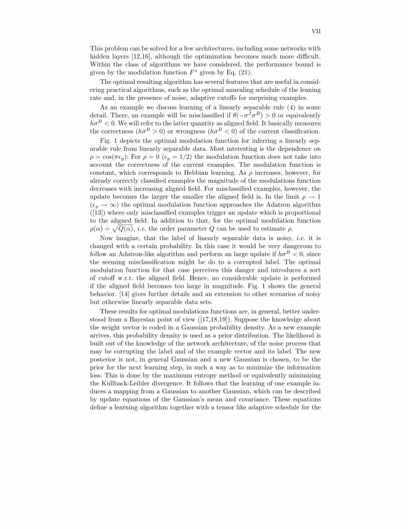
As an example we discuss learning of a linearly separable rule (4) in somedetail. There, an example will be misclassified if θ(−σJσB) > 0 or equivalentlyhσB < 0. We will refer to the latter quantity as aligned field. It basically measuresthe correctness (hσB > 0) or wrongness (hσB < 0) of the current classification.

Fig. 1 depicts the optimal modulation function for inferring a linearly sep-arable rule from linearly separable data. Most interesting is the dependence onρ = cos(πǫg): For ρ = 0 (ǫg = 1/2) the modulation function does not take intoaccount the correctness of the current examples. The modulation function isconstant, which corresponds to Hebbian learning. As ρ increases, however, foralready correctly classified examples the magnitude of the modulations functiondecreases with increasing aligned field. For misclassified examples, however, theupdate becomes the larger the smaller the aligned field is. In the limit ρ → 1(ǫg → ∞) the optimal modulation function approaches the Adatron algorithm([13]) where only misclassified examples trigger an update which is proportionalto the aligned field. In addition to that, for the optimal modulation functionρ(α) =

√

Q(α), i.e. the order parameter Q can be used to estimate ρ.

Now imagine, that the label of linearly separable data is noisy, i.e. it ischanged with a certain probability. In this case it would be very dangerous tofollow an Adatron-like algorithm and perform an large update if hσB < 0, sincethe seeming misclassification might be do to a corrupted label. The optimalmodulation function for that case perceives this danger and introduces a sortof cutoff w.r.t. the aligned field. Hence, no considerable update is performedif the aligned field becomes too large in magnitude. Fig. 1 shows the generalbehavior. [14] gives further details and an extension to other scenarios of noisybut otherwise linearly separable data sets.

These results for optimal modulations functions are, in general, better under-stood from a Bayesian point of view ([17,18,19]). Suppose the knowledge aboutthe weight vector is coded in a Gaussian probability density. As a new examplearrives, this probability density is used as a prior distribution. The likelihood isbuilt out of the knowledge of the network architecture, of the noise process thatmay be corrupting the label and of the example vector and its label. The newposterior is not, in general Gaussian and a new Gaussian is chosen, to be theprior for the next learning step, in such a way as to minimize the informationloss. This is done by the maximum entropy method or equivalently minimizingthe Kullback-Leibler divergence. It follows that the learning of one example in-duces a mapping from a Gaussian to another Gaussian, which can be describedby update equations of the Gaussian’s mean and covariance. These equationsdefine a learning algorithm together with a tensor like adaptive schedule for the

VIII

F ∗σB/√

Q

hσBhσB

Fig. 1. Left: Optimal modulation function F ∗ for learning a linearly separable classifi-cation of type (4) for various values of the order parameter ρ. Right: In addition to (4)the labels σB are subject to noise, ı.e. are flipped with probability λ. The aligned fieldhσB is a measure of the agreement of the classification of the current example with thegiven label. In both cases, all examples are weighted equally for ρ = 0 irrespective of thevalue of the aligned field hσB . This corresponds to Hebbian learning. In the noiselesscase (λ = 0) examples with a negative aligned field receive more weight as ρ increaseswhile those with positive aligned field gain less weight. For λ > 0 also examples withlarge negative aligned fields are not taken into account for updating. These examplesare most likely affected by the noise and therefore are deceptively misclassified. Theoptimal weight function possesses a cutoff value at negative values of hσB . This cutoffdecreases in absolute value with increasing λ and ρ.

learning rate. This algorithms are closely related to the variational algorithmdefined above. The Bayesian method has the advantage of being more general.It can also be readily applied to other cases where the Gaussian prior is notadequate [19].

In the following sections we follow the developments of these techniques inother directions. We first look into networks with hidden layers, since the expe-rience gained in studying on-line learning in these more complex architectureswill be important to better understand the application of on-line learning to theproblem of clustering.

3 On-line Learning in Two-Layered Networks

Classifiers such as (4) are the most fundamental learning networks. In termsof network architecture the next generalization are networks with one layer ofhidden units and a fixed hidden-to-output relation. An important example isthe so-called committee machine, where the overall output is determined by amajority vote of several classifiers of type (4). For such networks the variationalapproach of the previous section can be readily applied [12,16].

General two-layered networks, however, have variable hidden-to-output weightsand are “soft classifiers”, i.e. have continuous transfer functions. They consist

IX

of a layer of N inputs, a layer of K hidden units, and a single output. Theparticular input-output relation is given by

σ(ξ) =

K∑

i=1

wig(J i · ξ). (24)

Here, Ji denotes the N -dimensional weight vector of the i-th input branch andwi the weight connecting the i-th hidden unit with the output. For a (soft)committee machine, wi ≡ 0 for all branches i. Often, the number K of hiddenweight vectors Ji is chosen as K ≪ N . In fact, most analyses specialize onK = O(1). This restriction will also be pursued here. Note that the overalloutput is linear in wi, in contrast to the outputs of the hidden layer which ingeneral depend nonlinearly on the weights Ji via the transfer function g.

The class of networks (24) is of importance for several reasons: Firstly, theycan realize more complex classification schemes. Secondly, they are commonlyused in practical applications. Finally, two-layered networks with a linear outputare known to be universal approximators [20].

Analogously to section 2 the network (24) is trained by a sequence of uncor-related examples {(ξν , τν)} which are provided by an unknown rule τ(ξ) by theenvironment. As above, the example input vectors are denoted by ξµ, while hereτµ is the corresponding correct rule output.

In a commonly studied scenario the rule is provided by a network of the samearchitecture with hidden layer weights Bi, hidden-to-output weights vi, and anin general different number of hidden units M :

τ(ξ) =

M∑

k=1

vkg(Bk · ξ). (25)

In principle, the network (24) can implement such a function if K ≥ M .As in (9) the change of a weight is usually taken proportional to the input

of the corresponding layer in the network, i.e.

Jiµ+1 = Ji

µ +1

NFiξ

µ+1 (26)

wµ+1i = wµ

i +1

NFwg(Ji · ξµ+1). (27)

Again, the modulation functions Fi, Fw will in general depend on the recentlyprovided information (ξµ, τµ) and the current weights.

Note, however, that there is an asymmetry between the updates of Ji and wi.The change of the former is O(1/N) due to |ξ2| = O(N). As

∑Ki=1 g2(Ji · ξ) =

O(K) a change of the latter according to

wµ+1i = wµ

i +1

KFwg(Ji · ξµ+1). (28)

seems to be more reasonable. For reasons that will become clear below we willprefer a scaling with 1/N as in (27) over a scaling with 1/K, at least for thetime being.

X

Also note from (24, 25) that the stochastic dynamics of Ji and wi only de-pends on the fields hi = Ji ·ξ, bk = Bk ·ξ which can be viewed as a generalizationof (ref to eq 5). As in section 2, for large N these become Gaussian variables.Here, they have zero means and correlations

〈hihj〉 = Ji ·Jj =: Qij , 〈bkbl〉 = Bk ·Bl =: Tkl , 〈hibk〉 = Ji ·Bk =: Rik, (29)

where i, j = 1 . . . K and k, l = 1 . . . M .Introducing α = µ/N as above, the discrete dynamics (26, 27) can be replaced

by a set of coupled differential equations for Rik, Qij , and wi in the limit oflarge N : Projecting (26) into Bk and Jj , respectively, and averaging over therandomness of ξ leads to

dRik

dα= 〈Fibk〉 (30)

dQij

dα= 〈Fihj + Fjhi + FiFj〉, (31)

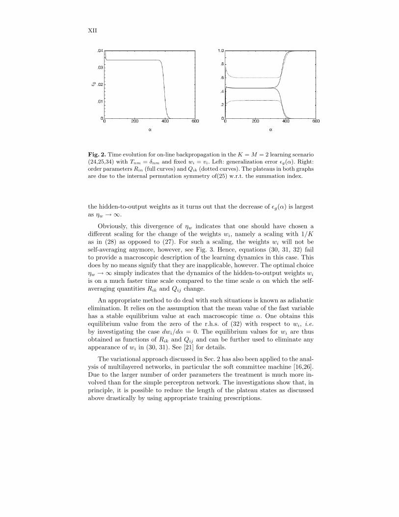
where the average is now with respect to the fields {hi} and {bk}. Hence, themicroscopic stochastic dynamics of O(K ·N) many weights Ji is replaced by themacroscopic dynamics of O(K2) many order parameters Rik and Qij , respec-tively. Again, these order parameters are self-averaging, i.e. their fluctuationsvanish as N → ∞. Fig. 3 exemplifies this for a specific dynamics.

The situation is somewhat different for the hidden-to-output weights wi. Inthe transition from microscopic, stochastic dynamics to macroscopic, averageddynamics the hidden-layer weights Ji are compressed to order parameters whichare scalar products, cf. (29). The hidden-to-output weights, however, are notcompressed into new parameters of the form of scalar products. (Scalar productsof the type

∑

i wivi do not even exist for K 6= M .) Scaling the update of wi by1/N as in (27) allows to replace 1/N by the differential dα as N → ∞. Hence,the averaged dynamics of the hidden-to-output weight reads

dwi

dα= 〈Fwg(hi)〉. (32)

Note that the r.h.s. of these differential equations depend on Rik, Qij via (29)and, hence, are coupled to the differential equations (30, 31) of these orderparameters as well. So in total, the macroscopic description of learning dynamicsconsists of the coupled set (30, 31, 32).

It might be surprising that the hidden-to-output weights wi by themselvesare appropriate for a macroscopic description while the hidden weights Ji arenot. The reason for this is twofold. First, the number K of wi had been taken tobe O(1), i.e. it does not scale with the dimension of inputs N . Therefore, thereis no need to compress a large number of microscopic variables into a smallnumber of macroscopic order parameters as for the Ji. Second, the change in wi

had been chosen to scale with 1/N . For this choice one can show that like Rik

and Qij the weights wi are self-averaging.

XI

For a given rule τ(ξ) to be learned, the generalization error is

ǫg({Ji, wi}) = 〈ǫ({Ji, wi})〉ξ, (33)

where ǫ({Ji, wi}) = 12 (σ − τ)2 is the instantaneous error. As the outputs σ and

τ depend on ξ only via the fields {hi} and {bk}, respectively, the average over ξ

can be replaced by an average over these fields. Hence, the generalization erroronly depends on order parameters Rik, Qij , wi as well as on Tkl and vk.

In contrast to section 2 it is a difficult task to derive optimal algorithms by avariational approach, since the generalization error (33) is a function of severalorder parameters. Therefore on-line dynamics in two-layer networks has mostlybeen studied in the setting of heuristic algorithms, in particular for backpropa-gation. There, the update of the weights is taken proportional to the gradient ofthe instantaneous error ǫ = ǫ({Ji, wi}) = 1

2 (σ − τ)2 with respect to the weights:

Jiµ+1 = Ji

µ − ηJ

N∇Ji

ǫ (34)

wµ+1i = wµ

i − ηw

N

∂ǫ

∂wi(35)

The parameters ηJ and ηw denote learning rates which scale the size of theupdate along the gradient of the instantaneous error. In terms of (26, 27) back-propagation corresponds to the special choices FJ = −ηJ(σ − τ)wig

′(hi) andFw = −ηw(σ−τ). A common choice for the transfer function is g(x) = erf(x/

√2).

With this specific choice, the averaging in the equations of motion (30, 31, 32)can be performed analytically for general K and M [22,23,24]

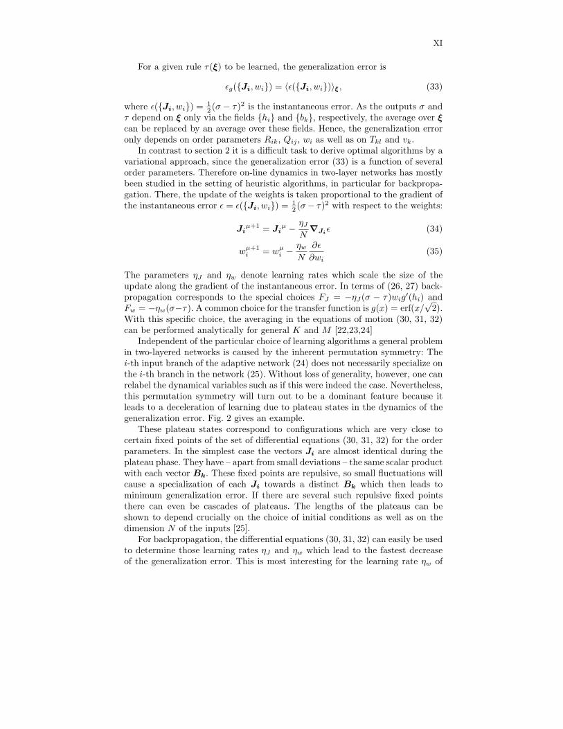
Independent of the particular choice of learning algorithms a general problemin two-layered networks is caused by the inherent permutation symmetry: Thei-th input branch of the adaptive network (24) does not necessarily specialize onthe i-th branch in the network (25). Without loss of generality, however, one canrelabel the dynamical variables such as if this were indeed the case. Nevertheless,this permutation symmetry will turn out to be a dominant feature because itleads to a deceleration of learning due to plateau states in the dynamics of thegeneralization error. Fig. 2 gives an example.

These plateau states correspond to configurations which are very close tocertain fixed points of the set of differential equations (30, 31, 32) for the orderparameters. In the simplest case the vectors Ji are almost identical during theplateau phase. They have – apart from small deviations – the same scalar productwith each vector Bk. These fixed points are repulsive, so small fluctuations willcause a specialization of each Ji towards a distinct Bk which then leads tominimum generalization error. If there are several such repulsive fixed pointsthere can even be cascades of plateaus. The lengths of the plateaus can beshown to depend crucially on the choice of initial conditions as well as on thedimension N of the inputs [25].

For backpropagation, the differential equations (30, 31, 32) can easily be usedto determine those learning rates ηJ and ηw which lead to the fastest decreaseof the generalization error. This is most interesting for the learning rate ηw of

XII

Fig. 2. Time evolution for on-line backpropagation in the K = M = 2 learning scenario(24,25,34) with Tnm = δnm and fixed wi = vi. Left: generalization error ǫg(α). Right:order parameters Rin (full curves) and Qik (dotted curves). The plateaus in both graphsare due to the internal permutation symmetry of(25) w.r.t. the summation index.

the hidden-to-output weights as it turns out that the decrease of ǫg(α) is largestas ηw → ∞.

Obviously, this divergence of ηw indicates that one should have chosen adifferent scaling for the change of the weights wi, namely a scaling with 1/Kas in (28) as opposed to (27). For such a scaling, the weights wi will not beself-averaging anymore, however, see Fig. 3. Hence, equations (30, 31, 32) failto provide a macroscopic description of the learning dynamics in this case. Thisdoes by no means signify that they are inapplicable, however. The optimal choiceηw → ∞ simply indicates that the dynamics of the hidden-to-output weights wi

is on a much faster time scale compared to the time scale α on which the self-averaging quantities Rik and Qij change.

An appropriate method to do deal with such situations is known as adiabaticelimination. It relies on the assumption that the mean value of the fast variablehas a stable equilibrium value at each macroscopic time α. One obtains thisequilibrium value from the zero of the r.h.s. of (32) with respect to wi, i.e.

by investigating the case dwi/dα = 0. The equilibrium values for wi are thusobtained as functions of Rik and Qij and can be further used to eliminate anyappearance of wi in (30, 31). See [21] for details.

The variational approach discussed in Sec. 2 has also been applied to the anal-ysis of multilayered networks, in particular the soft committee machine [16,26].Due to the larger number of order parameters the treatment is much more in-volved than for the simple perceptron network. The investigations show that, inprinciple, it is possible to reduce the length of the plateau states as discussedabove drastically by using appropriate training prescriptions.

XIII

1/√

N 1/√

N

Fig. 3. Finite size analysis of the order parameters R (△), Q (2) and w (◦, right panel)in the dynamics (34,35) for the special case K=M=1. Shown are the observed standarddeviations as a function of the system size for a fixed value of α. Each point depicts anaverage taken over 100 simulation runs. As can be seen, R and Q become selfaveragingin the thermodynamic limit N → ∞, i.e. their fluctuations vanish in this limit. Incontrast to that, the fluctuations of w remain finite if one optimizes the learning rateηw, which leads to the divergence ηw → ∞.

4 Dynamics of prototype based learning

In all training scenarios discussed above, the consideration of isotropic, i.i.d.input data yields non-trivial insights, already. The key information is containedin the training labels and, for modeling purposes, we have assumed that theyare provided by a teacher network.

In practical situations one would clearly expect the presence of structures ininput space, e.g. in the form of clusters which are more or less correlated withthe target function. Here we briefly discuss how the theoretical framework hasbeen extended in this direction. We will address, mainly, supervised learningschemes which detect or make use of structures in input space. Unsupervisedlearning from unlabeled, structured data has been treated along the very samelines but will not be discussed in detail, here. We refer to, for instance, [27,28]for overviews and [34,35,38,43,45] for example results in this context.

We will focus on prototype based supervised learning schemes which take intoaccount label information. The popular Learning Vector Quantization algorithm[32] and many of its variants follow the lines of competitive learning. Howeverthe aim is to obtain prototypes as typical representatives of their classes whichparameterize a distance based classification scheme.

LVQ algorithms can be treated within the same framework as above. Theanalysis requires only slight modifications due to the assumption of a non-trivialinput densities.

Several possibilities to model anisotropy in input space have been consideredin the literature, a prominent example being unimodal Gaussians with distinctprincipal axes [30,29,34,35]. Here, we focus on another simple but non-trivial

XIV

-2 0 2 4

-2

0

2

4

b+

b−

-4 -2 0 2 4-4

-2

0

2

4

h+

h−

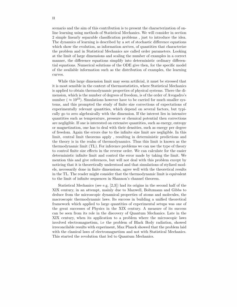
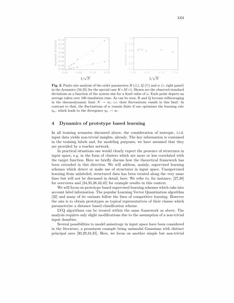
Fig. 4. Data as generated according to the density (36) in N = 200 dimensions withexample parameters p− = 0.6, p+ = 0.4, v− = 0.64, and v+ = 1.44. The open (filled)circles represent 160 (240) vectors ξ from clusters centered about orthonormal vectorsℓB+ (ℓB−) with ℓ = 1, respectively. The left panel displays to the projections b± =B± · ξ and diamonds mark the position of the cluster centers. The right panel showsprojections h± = w± ·ξ of the same data on a randomly chosen pair of orthogonal unitvectors w±.

model density: we assume feature vectors are generated independently accordingto a mixture of isotropic Gaussians:

P (ξ)=∑

σ=±1

pσP (ξ | σ) with P (ξ | σ) =1

√2πvσ

Nexp

[

− 1

2 vσ(ξ − ℓBσ)

2

]

.

(36)The conditional densities P (ξ | σ = ±1) correspond to clusters with variancesvσ centered at ℓBσ. For convenience, we assume that the vectors Bσ are or-thonormal: B2

σ = 1 and B+ ·B− = 0. The first condition sets only the scale onwhich the parameter ℓ controls the cluster offset. The orthogonality conditionfixes the position of cluster centers with respect to the origin in feature spacewhich could be chosen arbitrarily. Similar densities have been considered in, forinstance, [31,37,38,39,40].

In the context of supervised Learning Vector Quantization, see next section,we will assume that the target classification coincides with the cluster member-ship label σ for each vector ξ. Due to the significant overlap of clusters, this taskis obviously not linear separable.

Note that linearly separable rules defined for bimodal input data similar to(36) have been studied in [36]. While transient learning curves of the perceptroncan differ significantly from the technically simpler case of isotropic inputs, themain results concerning the (α → ∞)–asymptotic behavior persist.

Learning Vector Quantization (LVQ) a particularly intuitive and powerfulfamily of algorithms which has been applied in a variety of practical problems

XV

[41]. LVQ identifies prototypes, i.e. typical representatives of the classes in featurespace which then parameterize a distance based classification scheme.

Competitive learning schemes have been suggested in which a set of prototypevectors is updated from a sequence of example data. We will restrict ourselvesto the simplest non-trivial case of two prototypes w+,w− ∈ IRN and datagenerated according to a bi-modal distribution of type (36).

Most frequently a nearest prototype scheme is implemented: For classificationof a given input ξ, the distances

ds(ξ) = (ξ − ws)2, s = ±1 (37)

are determined and ξ is assigned to class +1 if d+(ξ) ≤ d−(ξ) and to class−1 else. The (squared) Euclidean distance (37) appears to be a natural choice.In practical situations, however, it can lead to inferior performance and theidentification of an appropriate distance or similarity measure is one of the keyissues in applications of LVQ.

A simple two prototype system as described above parameterizes a linearlyseparable classifier, only. However, we will consider learning of a non-separablerule where non-trivial effects of the prototype dynamics can be studied in thissimple setting already. Extensions to more complex models with several proto-types, i.e. piecewise linear decision boundaries and multi-modal input densitiesare possible but non-trivial, see [45] for a recent example.

Generically, LVQ algorithms perform updates of the form

wµ+1s = wµ

s +η

Nf(dµ

+, dµ−, s, σµ) (ξµ − wµ

s ) . (38)

Hence, prototypes are either moved towards or away from the current input.Here, the modulation function f controls the sign and, together with an explicitlearning rate η, the magnitude of the update.

So–called Winner-Takes-All (WTA) schemes update only the prototype whichis currently closest to the presented input vector. A prominent example of su-pervised WTA learning is Kohonen’s original formulation, termed LVQ1 [32,33].In our model scenario it corresponds to Eq. (38) with

f(dµ+, dµ

−, s, σµ) = Θ(dµ−s − dµ

+s) s σµ (39)

The Heaviside function singles out the winning prototype, and the products σµ = +1(−1) if the labels of prototype and example coincide (disagree).

For the formal analysis of the training dynamics, we can proceed in completeanalogy to the previously studied cases of perceptron and layered neural net-works. A natural choice of order parameters are the self- and cross-overlaps ofthe involved N -dimensional vectors:

Rsσ = ws · Bσ and Qst = ws · wt with σ, s, t ∈ {−1,+1} (40)

While these definitions are formally identical with Eq. (29), the role of the ref-erence vectors Bσ is not that of teacher vectors, here.

XVI

Following the by now familiar lines we obtain a set of coupled ODE of theform

dRSτ

dα= η (〈bτ fS〉 − RSτ 〈fS〉)

dQST

dα= η (〈hS fT + hT fS〉 − QST 〈fS + fT 〉)

+η2∑

σ=±1

vσpσ 〈fS fT 〉σ . (41)

Here, averages 〈. . .〉 over the full density P (ξ), Eq. (36) have to be evaluatedas appropriate sums over conditional averages 〈. . .〉σ corresponding to ξ drawnfrom cluster σ:

〈. . .〉 = p+ 〈. . .〉+ + p− 〈. . .〉− .

For a large class of LVQ modulation functions, the actual input ξµ appearson the right hand side of Eq. (41) only through its length and the projections

hs = ws · ξ and bσ = Bσ · ξ (42)

where we omitted indices µ but implicitly assume that the input ξ is uncorrelatedwith the current prototypes ws. Note that also Heaviside terms as in Eq. (39)do not depend on ξ explicitly, for example:

Θ (d− − d+) = Θ [+2(h+ − h−) − Q++ + Q−−] .

When performing the average over the actual example ξ we first exploit the factthat

limN→∞

⟨

ξ2⟩

/N = (v+p+ + v−p−)

for all input vectors in the thermodynamic limit. Furthermore, the joint Gaussiandensity P (hµ

+, hµ−, bµ

+, bµ−) can be expressed as a sum over contributions from

the clusters. The respective conditional densities are fully specified by first andsecond moments

〈hs〉σ = ℓRsσ, 〈bτ 〉σ = ℓδτσ, 〈hsht〉σ − 〈hs〉σ 〈ht〉σ = vσ Qst

〈hsbτ 〉σ − 〈hs〉σ 〈bτ 〉σ = vσ Rsτ , 〈bρbτ 〉σ − 〈bρ〉σ 〈bτ 〉σ = vσ δρτ (43)

where s, t, σ, ρ, τ ∈ {+1,−1} and δ... is the Kronecker-Delta. Hence, the densityof h± and b± is given in terms of the model parameters ℓ, p±, v±, and the abovedefined set of order parameters in the previous time step.

After working out the system of ODE for a specific modulation function, itcan be integrated, at least numerically. Here we consider prototypes that areinitialized as independent random vectors of squared length Q with no priorknowledge about the cluster positions. In terms of order parameters this impliesin our simple model

Q++(0) = Q−−(0) = Q, and Q+−(0) = RSσ(0) = 0 for all S, σ. (44)

XVII

As in any supervised scenario, the success of learning is to be quantified interms of the generalization error. Here we have to consider two contributions formisclassifying data from cluster σ = 1 or σ = −1 separately:

ǫ = p+ ǫ+ + p− ǫ− with ǫσ = 〈Θ (d+σ − d−σ)〉σ . (45)

Exploiting the central limit theorem in the same fashion as above, one obtainsfor the above contributions ǫ±:

ǫσ = Φ

(

Qσσ − Q−σ−σ − 2ℓ(Rσσ − R−σσ)

2√

vσ

√

Q++ − 2Q+− + Q−−

)

(46)

where Φ(z) =∫ z

−∞dx e−x2/2/

√2π.

By inserting {RSσ(α), QST (α)} we obtain the learning curve ǫg(α), i.e. thetypical generalization error after on-line training with α N random examples.Here, we once more exploit the fact that the order parameters and, thus, also ǫg

are self-averaging non-fluctuating quantities in the thermodynamic limit N →∞.

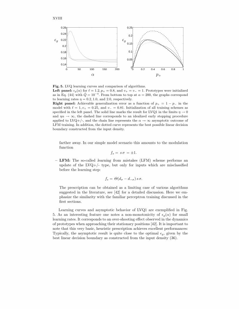
As an example, we consider the dynamics of LVQ1, cf. Eq. (39). Fig. 5 (leftpanel) displays the learning curves as obtained for a particular setting of themodel parameters and different choices of the learning rate η. Initially, a largelearning rate is favorable, whereas smaller values of η facilitate better gener-alization behavior at large α. One can argue that, as in stochastic gradientdescent procedures, the best asymptotic ǫg will be achieved for small learningrates η → 0. In this limit, we can omit terms quadratic in η from the differentialequations and integrate them directly in rescaled time (ηα). The asymptotic,stationary result for (ηα) → ∞ then corresponds to the best achievable per-formance of the algorithm in the given model settings. Figure 5 (right panel)displays, among others, an example result for LVQ1.

With the formalism outlined above it is readily possible to compare differ-ent algorithms within the same model situation. This concerns, for instance,the detailed prototype dynamics and sensitivity to initial conditions. Here, werestrict ourselves to three example algorithms and very briefly discuss essentialproperties and the achievable generalization ability:

– LVQ1: This basic prescription was already defined above as the originalWTA algorithm with modulation function

fs = Θ(d−s − d+s) s σ.

– LVQ+/-: Several modifications have been suggested in the literature, aim-ing at better generalization behavior. The term LVQ+/- is used here todescribe one basic variant which updates two vectors at a time: the closestamong all prototypes which belong to the same class (a) and the closest oneamong those that represent a different class (b). The so-called correct winner

(a) is moved towards the data while the wrong winner (b) is pushed even

XVIII

0 50 100 150 200

0.14

0.16

0.18

0.2

0.22

0.24

0.26

α

ǫg

0 0.2 0.4 0.6 0.8 10

0.05

0.1

0.15

0.2

0.25

p+

ǫg

Fig. 5. LVQ learning curves and comparison of algorithms.Left panel: ǫg(α) for ℓ = 1.2, p+ = 0.8, and v+ = v− = 1. Prototypes were initializedas in Eq. (44) with Q = 10−4. From bottom to top at α = 200, the graphs correspondto learning rates η = 0.2, 1.0, and 2.0, respectively.Right panel: Achievable generalization error as a function of p+ = 1 − p− in themodel with ℓ = 1, v+ = 0.25, and v− = 0.81. Initialization of all training schemes asspecified in the left panel. The solid line marks the result for LVQ1 in the limits η → 0and ηα → ∞, the dashed line corresponds to an idealized early stopping procedureapplied to LVQ+/-, and the chain line represents the α → ∞ asymptotic outcome ofLFM training. In addition, the dotted curve represents the best possible linear decisionboundary constructed from the input density.

farther away. In our simple model scenario this amounts to the modulationfunction

fs = s σ = ±1.

– LFM: The so-called learning from mistakes (LFM) scheme performs anupdate of the LVQ+/- type, but only for inputs which are misclassifiedbefore the learning step:

fs = Θ(dσ − d−σ) s σ.

The prescription can be obtained as a limiting case of various algorithmssuggested in the literature, see [42] for a detailed discussion. Here we em-phasize the similarity with the familiar perceptron training discussed in thefirst sections.

Learning curves and asymptotic behavior of LVQ1 are exemplified in Fig.5. As an interesting feature one notes a non-monotonicity of ǫg(α) for smalllearning rates. It corresponds to an over-shooting effect observed in the dynamicsof prototypes when approaching their stationary positions [42]. It is important tonote that this very basic, heuristic prescription achieves excellent performances:Typically, the asymptotic result is quite close to the optimal ǫg, given by thebest linear decision boundary as constructed from the input density (36).

XIX

The naive application of LVQ+/- training results in a strong instability: Inall settings with p+ 6= p−, the prototype representing the weaker class will bepushed away in the majority of training steps. Consequently, a divergent behav-ior is observed and, for α → ∞, the classifier assigns all data to the the strongercluster with the trivial result ǫg = min{p+, p−}. Several measures have been sug-gested to control the instability. In Kohonen’s LVQ2.1 and other modifications,example data are only accepted for update when ξ falls into a window close tothe current decision boundary. Another intuitive approach is based on the obser-vation that ǫg(α) generically displays a pronounced minimum before the general-ization behavior deteriorates. In our formal model, it is possible to work out thelocation of the minimum analytically and thus determine the performance of anidealized early stopping method. The corresponding result is displayed in Fig. 5(right panel, dashed line) and appears to compete well with LVQ1. However, itis important to note that the quality of the minimum in ǫg(α) strongly dependson the initial conditions. Furthermore, in a practical situation, successful earlystopping would require the application of costly validation schemes.

Finally, we briefly discuss the LFM prescription. A peculiar feature of LFMis that the stationary position of prototypes does depend strongly on the initialconfiguration [42]. On the contrary, the α → ∞ asymptotic decision boundaryis well-defined. In the LFM prescription, emphasis is on the classification; theaspect of Vector Quantization (representation of clusters) is essentially disre-garded. While at first sight clear and attractive, LFM yields a far from optimalperformance in the limit α → ∞. Note that already in perceptron training asdiscussed in the first sections, a naive learning from mistakes strategy is boundto fail miserably in general cases of noisy data or unlearnable rules.

The above considerations concern only the simplest LVQ training scenariosand algorithms. Several directions in which to extend the formalism are obviouslyinteresting.

We only mention that unsupervised prototype based learning has been treatedin complete analogy to the above [43,44]. Technically, it reduces to the consid-eration of modulation functions which do not depend on the cluster or classlabel. The basic competitive WTA Vector Quantization training would be repre-sented, for instance, by the modulation function fs = Θ(d−s−d+s) which alwaysmoves the winning prototype closer to the data. The training prescription canbe interpreted as a stochastic gradient descent of a cost function, the so-calledquantization error [44]. The exchange and permutation symmetry of prototypesin unsupervised training results in interesting effects which resemble the plateausdiscussed in multilayered neural networks, cf. section 3.

The consideration of a larger number of Gaussians contributing to the inputdensity is relatively simple. Thus, it is possible to model more complex datastructures and study their effect on the training dynamics. The treatment ofmore than two prototypes is also conceptually simple but constitutes a technicalchallenge. Obviously, the number of order parameters increases. In addition,the r.h.s. of the ODE cannot be evaluated analytically, in general, but involvenumerical integrals. Note that the dynamics of several prototypes representing

XX

the same class of data resembles strongly the behavior of unsupervised VectorQuantization. First results along these lines have been obtained recently, see forinstance [45].

The variational optimization, as discussed for the perceptron in detail, shouldgive insights into the essential features of robust and successful LVQ schemes.Due to the more complex input density, however, the analysis proves quite in-volved and has not yet been completed.

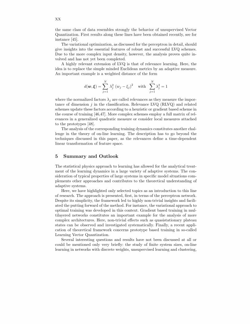
A highly relevant extension of LVQ is that of relevance learning. Here, theidea is to replace the simple minded Euclidean metrics by an adaptive measure.An important example is a weighted distance of the form

d(w, ξ) =

N∑

j=1

λ2j (wj − ξj)

2with

N∑

j=1

λ2j = 1

where the normalized factors λj are called relevances as they measure the impor-tance of dimension j in the classification. Relevance LVQ (RLVQ) and relatedschemes update these factors according to a heuristic or gradient based scheme inthe course of training [46,47]. More complex schemes employ a full matrix of rel-evances in a generalized quadratic measure or consider local measures attachedto the prototypes [48].

The analysis of the corresponding training dynamics constitutes another chal-lenge in the theory of on-line learning. The description has to go beyond thetechniques discussed in this paper, as the relevances define a time-dependentlinear transformation of feature space.

5 Summary and Outlook

The statistical physics approach to learning has allowed for the analytical treat-ment of the learning dynamics in a large variety of adaptive systems. The con-sideration of typical properties of large systems in specific model situations com-plements other approaches and contributes to the theoretical understanding ofadaptive systems.

Here, we have highlighted only selected topics as an introduction to this lineof research. The approach is presented, first, in terms of the perceptron network.Despite its simplicity, the framework led to highly non-trivial insights and facili-ated the putting forward of the method. For instance, the variational approach tooptimal training was developed in this context. Gradient based training in mul-tilayered networks constitutes an important example for the analysis of morecomplex architectures. Here, non-trivial effects such as quasistationary plateaustates can be observed and investigated systematically. Finally, a recent appli-cation of theoretical framework concerns prototype based training in so-calledLearning Vector Quantization.

Several interesting questions and results have not been discussed at all orcould be mentioned only very briefly: the study of finite system sizes, on-linelearning in networks with discrete weights, unsupervised learning and clustering,

XXI

training from correlated data or from a fixed pool of examples, query strategies,to name only a few. We can only refer to the list of references, in particular [27]and [28] may serve as a starting point for the interested reader.

Due to the conceptual simplicity of the approach and its applicability in awide range of contexts it will certainly continue to facilitate better theoreticalunderstanding of learning systems in general. Current challenges include thetreatment of non-trivial input distributions, the dynamics of learning in morecomplex networks architectures, the optimization of algorithms and their prac-tical implementation in such systems, or the investigation of component-wiseupdates as, for instance, in relevance LVQ.

References

1. Metropolis, N., Rosenbluth, A.W., Rosenbluth, M.N., Teller, A.H., Teller, E.: Equa-tions of State calculations by fast computing machines. J. Chem. Phys. 21, 1087(1953)

2. Huang, K.: Statistical Mechanics. Wiley and Sons, New York (1987)3. Jaynes, E.T.: Probability Theory: The Logic of Science. Bretthorst, G.L. (ed.),

Cambridge University Press, Cambridge, UK (2003)4. Mace, C.W.H., Coolen, T.: Dynamics of Supervised Learning with Restricted

Training Sets. Statistics and Computing 8, 55-88 (1998)5. Biehl, M., Schwarze, M.: On-line learning of a time-dependent rule Europhys. Lett.

20, 733-738 (1992)6. Biehl, M., Schwarze, H.: Learning drifting concepts with neural networks. Journal

of Physics A: Math. Gen. 26, 2651-2665 (1993)7. Kinouchi, O., Caticha, N.: Lower bounds on generalization errors for drifting rules.

J. Phys. A: Math. Gen.26, 6161-6171 (1993)8. Vicente, R, Kinouchi, O., Caticha, N.: Statistical Mechanics of Online Learning of

Drifting Concepts: A Variational Approach. Machine Learning 32, 179-201 (1998)9. Reents, G., Urbanczik, R.: Self-averaging and on-line learning. Phys. Rev. Lett.

80, 5445-5448 (1998)10. Kinzel, W., Rujan, P.: Improving a network generalization ability by selecting

examples. Europhys. Lett. 13, 2878 (1990)11. Kinouchi, O., Caticha, N.: Optimal generalization in perceptrons. J. Phys. A: Math.

Gen. 25, 6243-6250 (1992)12. Copelli, M., Caticha, N.: On-line learning in the committee machine. J. Phys. A:

Math. Gen. 28, 1615-1625 (1995)13. Biehl, M., Riegler, P.: On-line Learning with a Perceptron. Europhys. Lett. 78:

525-530 (1994)14. Biehl, M., Riegler, P., Stechert, M.: Learning from Noisy Data: An Exactly Solvable

Model. Phys. Rev. E 76, R4624-R4627 (1995)15. Copelli, M., Eichhorn, R., Kinouchi, O., Biehl, M., Simonetti, R., Riegler, P.,

Caticha, N.: Noise robustness in multilayer neural networks. Europhys. Lett. 37,427-432 (1995)

16. Vicente, R., Caticha, N.: Functional optimization of online algorithms in multilayerneural networks. J. Phys. A: Math. Gen. 30, L599-L605 (1997)

17. Opper, M.: A Bayesian approach to on-line learning. In: [27], pp. 363-378 (1998)18. Opper, M., Winther, O.: A mean field approach to Bayes learning in feed-forward

neural networks. Phys. Rev. Lett. 76, 1964-1967 (1996)

XXII

19. Solla, S.A., Winther, O.: Optimal perceptron learning: an online Bayesian ap-proach. In: [27], pp. 379-398 (1998)

20. Cybenko, G.V.: Approximation by superposition of a sigmoidal function. Math. ofControl, Signals and Systems 2, 303-314 (1989)

21. Endres, D., Riegler, P.: Adaptive systems on different time scales. J. Phys. A:Math. Gen. 32: 8655-9663 (1999)

22. Biehl, M., Schwarze, H.: Learning by on-line gradient descent. J. Phys A: Math.Gen. 28, 643 (1995)

23. Saad, D., Solla, S.A.: Exact solution for on-line learning in multilayer neural net-works. Phys. Rev. Lett. 74, 4337-4340 (1995)

24. Saad, D., Solla, S.A.: Online learning in soft committee machines. Phys. Rev. E52, 4225-4243 (1995)

25. Biehl, M., Riegler, P., Wohler, C.: Transient Dynamics of Online-learning in two-layered neural networks. J. Phys. A: Math. Gen. 29: 4769 (1996)

26. Saad, D, Rattray, M.: Globally optimal parameters for on-line learning in multilayerneural networks. Phys. Rev. Lett. 79, 2578 (1997)

27. Saad, D. (ed.): On-line learning in neural networks. Cambridge University Press,Cambridge, UK (1998)

28. Engel, A., Van den Broeck, C.: The Statistical Mechanics of Learning. CambridgeUniversity Press, Cambridge, UK (2001)

29. Schlosser, E., Saad, D., Biehl, M.: Optimisation of on-line Principal ComponentAnalysis. J. Physics A: Math. Gen. 32, 4061 (1999)

30. Biehl, M., Schlosser, E.: The dynamics of on-line Principal Component Analysis.J. Physics A: Math. Gen. 31: L97 (1998)

31. Biehl, M., Mietzner, A.: Statistical mechanics of unsupervised learning. Europhys.Lett. 27, 421-426 (1993)

32. Kohonen, T.: Self-Organizing Maps. Springer, Berlin (1997)33. Kohonen, T.: Learning vector quantization. In: Arbib, M.A. (ed.) The Handbook

of Brain Theory and Neural Networks., pp. 537-540. MIT Press, Cambridge, MA(1995)

34. Van den Broeck, C., Reimann, P.: Unsupervised Learning by Examples: On-lineVersus Off-line. Phys. Rev. Lett. 76, 2188-2191, (1996)

35. Reimann, P, Van den Broeck, C, Bex, G.J.: A Gaussian Scenario for UnsupervisedLearning. J. Phys. A: Math. Gen. 29, 3521-3533 (1996)

36. Riegler, P., Biehl, M., Solla, S.A., Marangi, C.: On-line learning from clusteredinput examples. In: Marinaro, M., Tagliaferri, R. (eds.) Neural Nets WIRN Vietri-

95, Proc. of the 7th Italian Workshop on Neural Nets, pp. 87-92. World Scientific,Singapore (1996)

37. Marangi, C., Biehl, M., Solla, S.A.: Supervised learning from clustered input ex-amples. Europhys. Lett. 30, 117-122 (1995)

38. Biehl, M.: An exactly solvable model of unsupervised learning. Europhysics Lett.25, 391-396 (1994)

39. Meir, R.: Empirical risk minimization versus maximum-likelihood estimation: acase study. Neural Computation 7, 144-157 (1995)

40. Barkai, N, Seung, H.S., Sompolinksy, H.: Scaling laws in learning of classificationtasks. Phys. Rev. Lett. 70, 3167-3170 (1993)

41. Neural Networks Research Centre. Bibliography on the self-organizing maps(SOM) and learning vector quantization (LVQ). Helsinki University of Technology,available on-line: http://liinwww.ira.uka.de/bibliography/Neural/SOM.LVQ.html(2002)

XXIII

42. Biehl, M, Ghosh, A., Hammer, B.: Dynamics and generalization ability of LVQalgorithms. J. Machine Learning Research 8, 323-360 (2007)

43. Biehl, M., Freking, A., Reents, G.: Dynamics of on-line competitive learning.Europhysics Letters 38, 73-78 (1997)

44. Biehl, M., Ghosh, A., Hammer, B.: Learning Vector Quantization: The Dynamicsof Winner-Takes-All algorithms. Neurocomputing 69, 660-670 (2006)

45. Witeolar, A., Biehl, M., Ghosh, A., Hammer, B.: Learning Dynamics of NeuralGas and Vector Quantization. Neurocomputing 71, 1210-1219 (2008)

46. Bojer, T., Hammer, B., Schunk, D., Tluk von Toschanowitz, K.: Relevance deter-mination in learning vector quantization. In: Verleysen, M. (ed.) European Sym-posium on Artificial Neural Networks ESANN 2001, pp. 271-276. D-facto publica-tions, Belgium (2001)

47. Hammer, B., Villmann, T.: Generalized relevance learning vector quantization.Neural Networks 15, 1059-1068 (2002)

48. Schneider, P, Biehl, M., Hammer, B.: Relevance Matrices in Learning Vector Quan-tization In: Verleysen, M. (ed.) European Symposium on Artificial Neural NetworksESANN 2007, pp. 37-43, d-side publishing, Belgium (2007)