Embed Size (px)
Citation preview
UNIVERSITY of ALBERTA
Linglong Kong
University of Alberta
Special Thanks to Professor Hongtu Zhu at UNC
ICSA Canada Chapter August 4, 2015 @ Calgary, AB
Statistical Methods for Neuroimaging Data Analysis ICSA Canada Chapter 2015 Lecture 2
Brain Connectivity Analysis

UNIVERSITY of ALBERTA
Reading materials: 1. Friston, K. J. (2009). Modalities, modes, and models in functional neuroimaging. Science
326, 399-403. 2. Rubinov, M. and Sporns, O. (2010). Complex network measures of brain connectivity:
Uses and interpretations. NeuroImage 52, 1059–1069. 3. Buckner, R. L., Andrews-Hanna, J. R. and Schacter, D. L. (2008). The brain’s default
network anatomy, function, and relevance to disease. Ann. N.Y. Acad. Sci. 1124: 1–38. 4. Honey, C.J., Thivierge, J.P., and Sporns, O. (2010). Can structure predict function in the
human brain? NeuroImage 52,766–776. 5. Buckner, R. L., Andrews-Hanna, J. R. and Schacter, D. L. (2008). The brain’s default
network anatomy, function, and relevance to disease. Ann. N.Y. Acad. Sci. 1124: 1–38. 6. Van Dijk, K. R. A., …, Buckner, R. L. (2010). Intrinsic functional connectivity as a tool for
human connectomics: theory, properties, and optimization. J. Neurophysiol. 103, 297-321.
Acknowledgement: Multiple slides were copied from Drs. Lindquist, Rowe, and Huettel, FSL, and SPM training materials.
UNIVERSITY of ALBERTA
Brain Connectivity
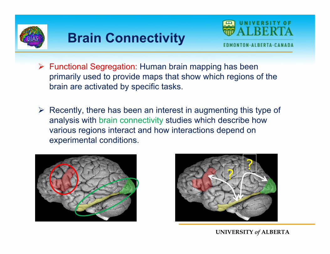
Ø Functional Segregation: Human brain mapping has been primarily used to provide maps that show which regions of the brain are activated by specific tasks.
Ø Recently, there has been an interest in augmenting this type of analysis with brain connectivity studies which describe how various regions interact and how interactions depend on experimental conditions.
? ?
UNIVERSITY of ALBERTA
Brain Networks
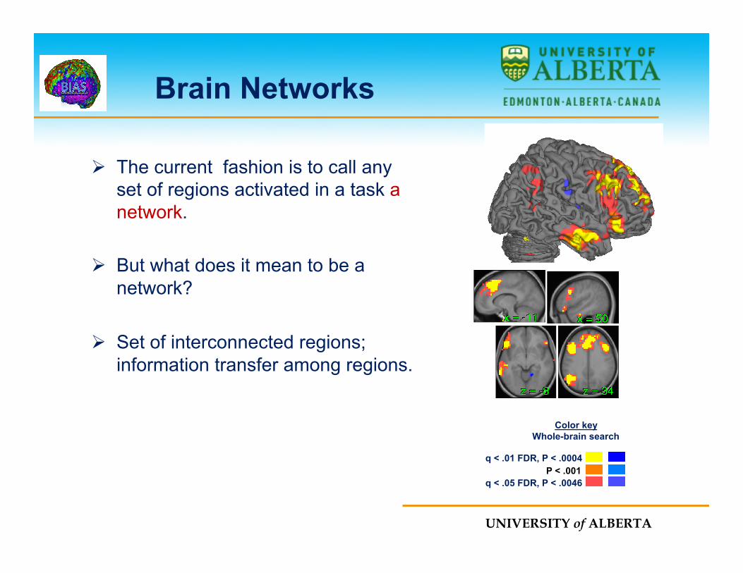
Ø The current fashion is to call any set of regions activated in a task a network.
Ø But what does it mean to be a network?
Ø Set of interconnected regions; information transfer among regions.
q < .01 FDR, P < .0004 P < .001
q < .05 FDR, P < .0046
Color key Whole-brain search
+ -
UNIVERSITY of ALBERTA
UNIVERSITY of ALBERTA
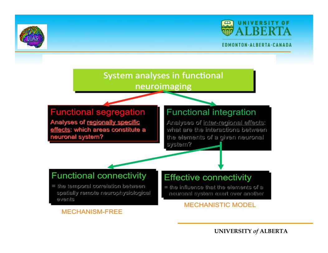
Functional Connectivity
Ø Functional connectivity is a statement about observed associations among regions and/or performance and physiological variables.
Ø It does not comment on how these associations are mediated.
Ø Functional connectivity analysis is usually performed using data-driven transformation methods which make no assumptions about the underlying biology.
UNIVERSITY of ALBERTA
Functional Connectivity
Ø Methods:
² Seed analyses
² Psychophysiological interaction analyses
² Principle Components Analysis
² Partial Least Squares
² Independent Components Analysis
UNIVERSITY of ALBERTA
Effective Connectivity
Ø Effective connectivity analysis is performed using statistical models which make anatomically motivated assumptions and restricts inference to networks comprising of a number of pre-selected regions of interest.
Ø These methods are hypothesis driven rather than data-driven and most applicable when it is possible to specify the relevant functional areas.
UNIVERSITY of ALBERTA
Effective Connectivity
Ø Methods:
² Structural Equation Modeling
² Granger Causality
² Dynamic Causal Modeling
• Note that Granger causality does not rely on an a priori specified structural model.

UNIVERSITY of ALBERTA
Functional Connectivity
UNIVERSITY of ALBERTA
Levels of Analysis
Ø Functional connectivity can be applied at different levels of analysis, with different interpretations at each.
Ø Connectivity across time can reveal networks that are dynamically activated across time.
Ø Connectivity across trials can identify coherent networks of task related activations.
Ø Connectivity across subjects can reveal patterns of coherent individual differences.
Ø Connectivity across studies can reveal tendencies for studies to co-activate within sets of regions.
UNIVERSITY of ALBERTA
Bivariate Connectivity
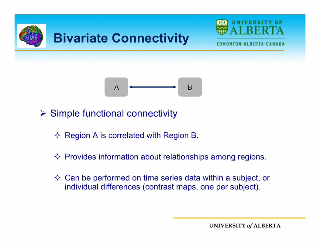
Ø Simple functional connectivity
² Region A is correlated with Region B.
² Provides information about relationships among regions.
² Can be performed on time series data within a subject, or individual differences (contrast maps, one per subject).
A B
UNIVERSITY of ALBERTA
Time Series Connectivity
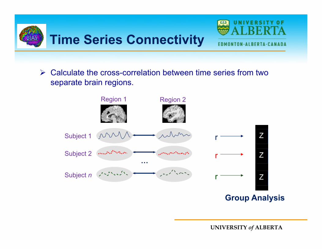
Ø Calculate the cross-correlation between time series from two separate brain regions.
Region 1 Region 2
Subject 1
Subject 2
Subject n
…
Group Analysis
r Z
r Z
r Z
Z
Z
Z
UNIVERSITY of ALBERTA
Seed Analysis
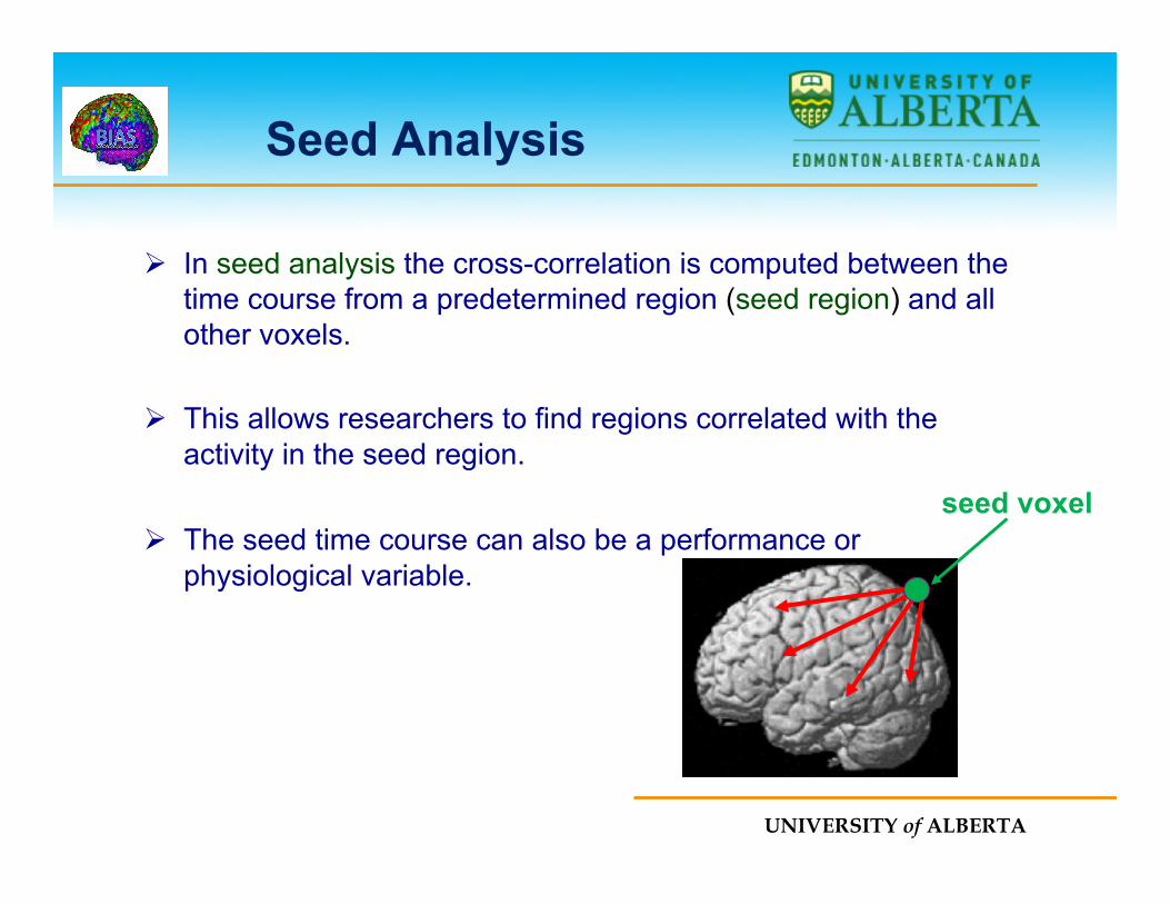
Ø In seed analysis the cross-correlation is computed between the time course from a predetermined region (seed region) and all other voxels.
Ø This allows researchers to find regions correlated with the activity in the seed region.
Ø The seed time course can also be a performance or physiological variable.
seed voxel
UNIVERSITY of ALBERTA
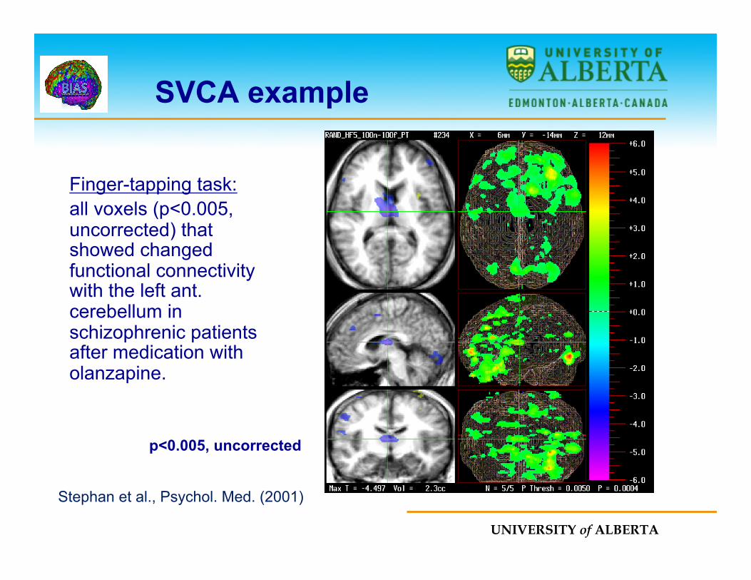
SVCA example
Finger-tapping task: all voxels (p<0.005, uncorrected) that showed changed functional connectivity with the left ant. cerebellum in schizophrenic patients after medication with olanzapine.
Stephan et al., Psychol. Med. (2001)
p<0.005, uncorrected
UNIVERSITY of ALBERTA
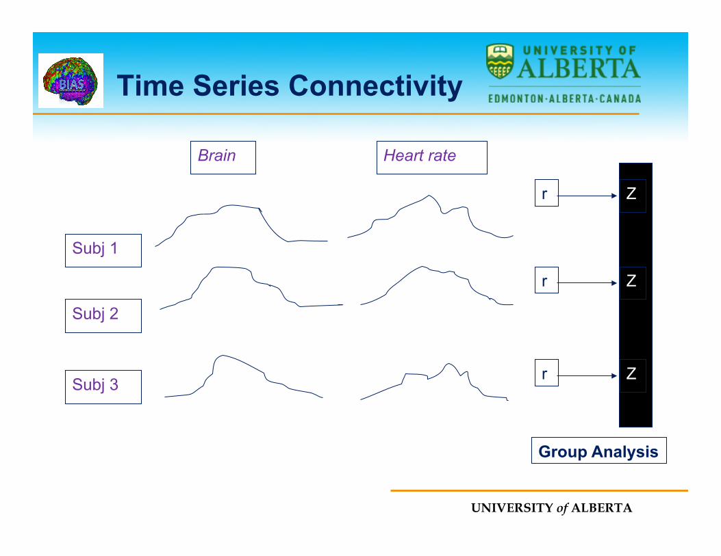
Group Analysis
Time Series Connectivity
Brain Heart rate
Subj 1
Subj 2
Subj 3
r Z
r Z
r Z
UNIVERSITY of ALBERTA
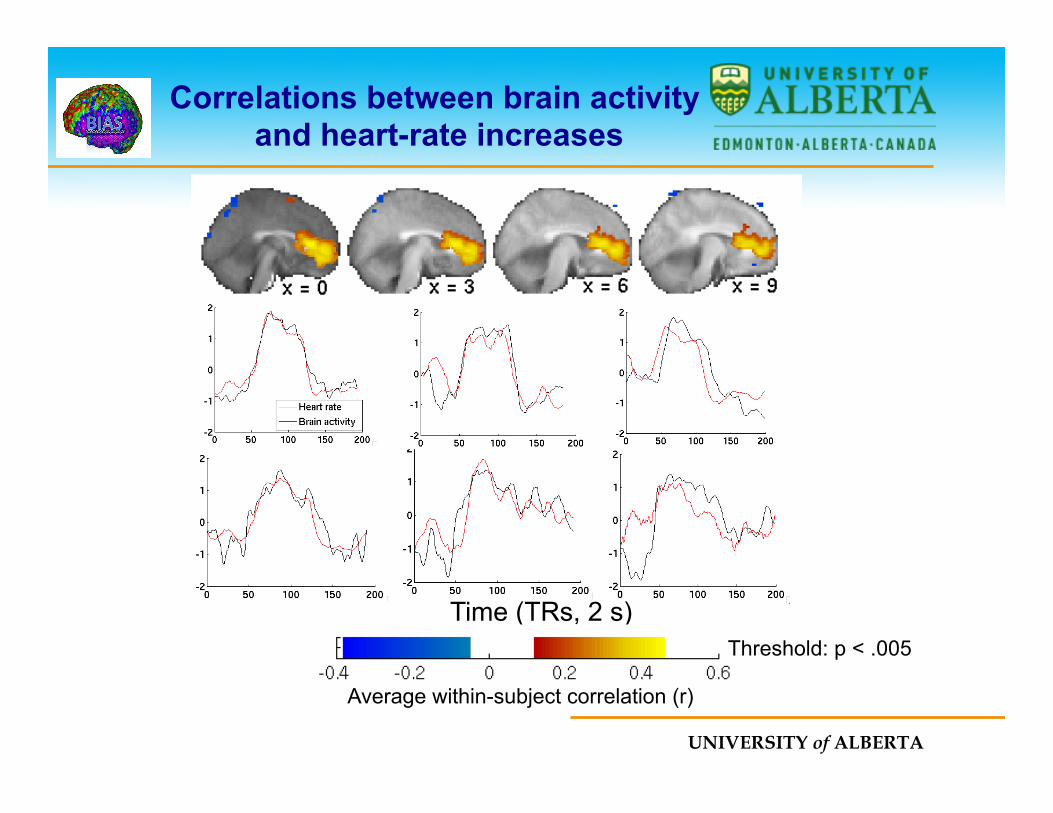
Correlations between brain activity and heart-rate increases
Time (TRs, 2 s)
Average within-subject correlation (r)
Threshold: p < .005
UNIVERSITY of ALBERTA
Issues
Ø One of the main problems with time series connectivity is the fact that there may be different hemodynamic lags in different regions:
² Time series from different regions may not match up, even if neural activity patterns match up.
² If lags are estimated from data, temporal order may be caused by vascular (uninteresting) or neural (interesting) response.
UNIVERSITY of ALBERTA
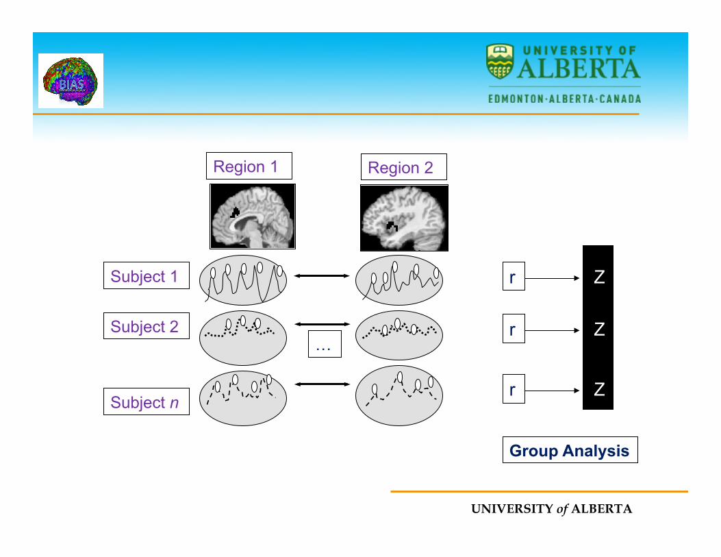
Beta Series
Ø The beta series approach can be used to minimize issues of inter-region neurovascular coupling.
Ø Procedure:
² Fit a GLM to obtain separate parameter estimates for each individual trial.
² Compute the correlation between these estimates across voxels.
UNIVERSITY of ALBERTA
Region 1 Region 2
Subject 1
Subject 2
Subject n
…
Group Analysis
r Z
r Z
r Z
UNIVERSITY of ALBERTA
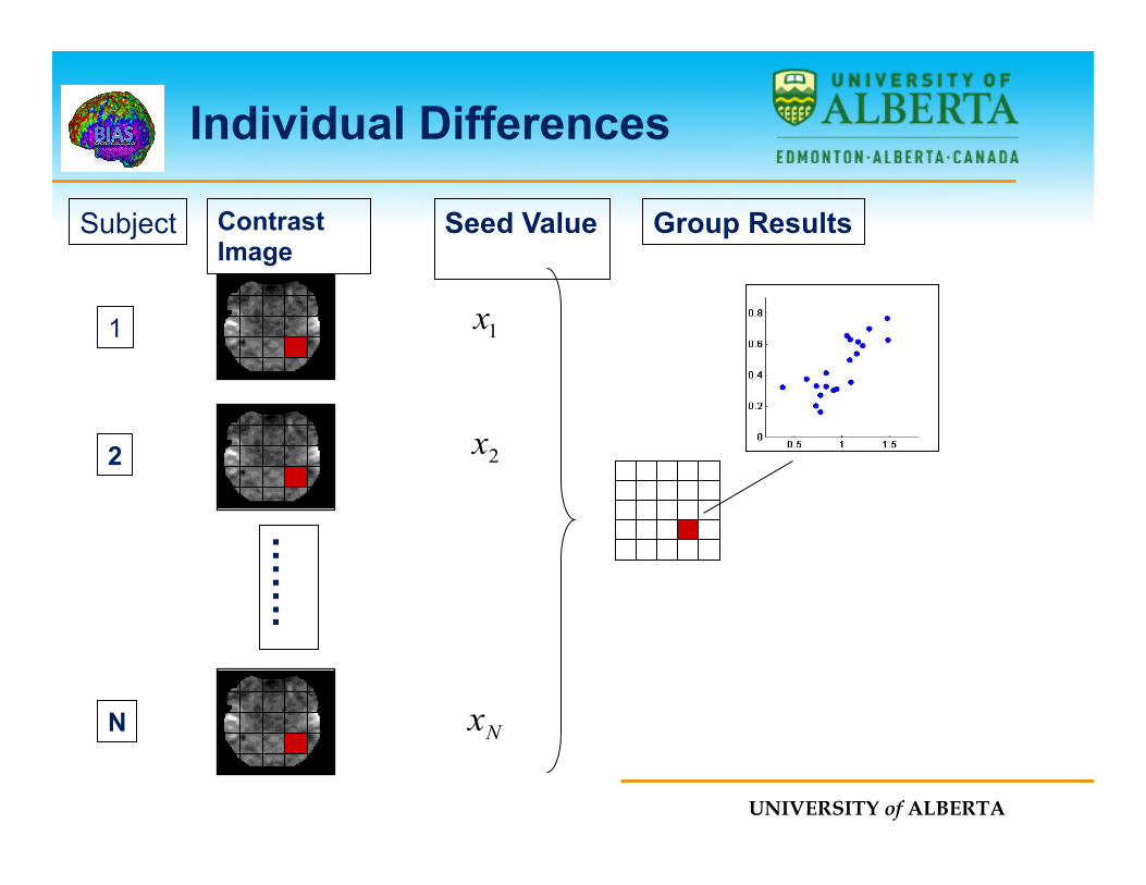
Individual Differences
……
..
Subject Contrast Image
1
2
N
Seed Value
1x
2x
Nx
Group Results
UNIVERSITY of ALBERTA
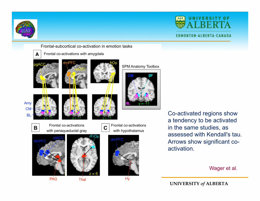
Co-activation across Studies
Ø Meta-analysis can be used to reveal patterns of co-activated regions.
Ø If two regions are co-activated, studies that activate one region are more likely to activate the other region as well.
Ø Co-activation is thus a meta-analytic analogue to functional connectivity analyses in individual neuroimaging studies.
UNIVERSITY of ALBERTA
Co-activated regions show a tendency to be activated in the same studies, as assessed with Kendall's tau. Arrows show significant co-activation.
Wager et al.
UNIVERSITY of ALBERTA
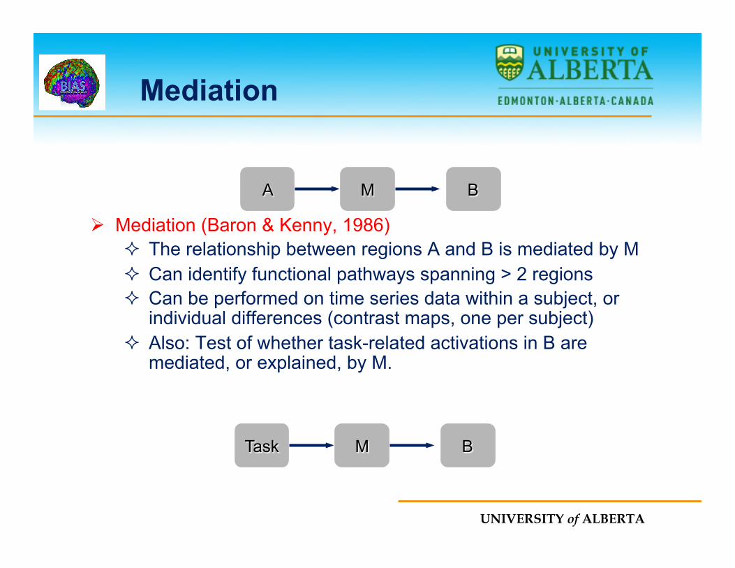
Mediation
Ø Mediation (Baron & Kenny, 1986) ² The relationship between regions A and B is mediated by M ² Can identify functional pathways spanning > 2 regions ² Can be performed on time series data within a subject, or
individual differences (contrast maps, one per subject) ² Also: Test of whether task-related activations in B are
mediated, or explained, by M.
A B M
Task B M
UNIVERSITY of ALBERTA
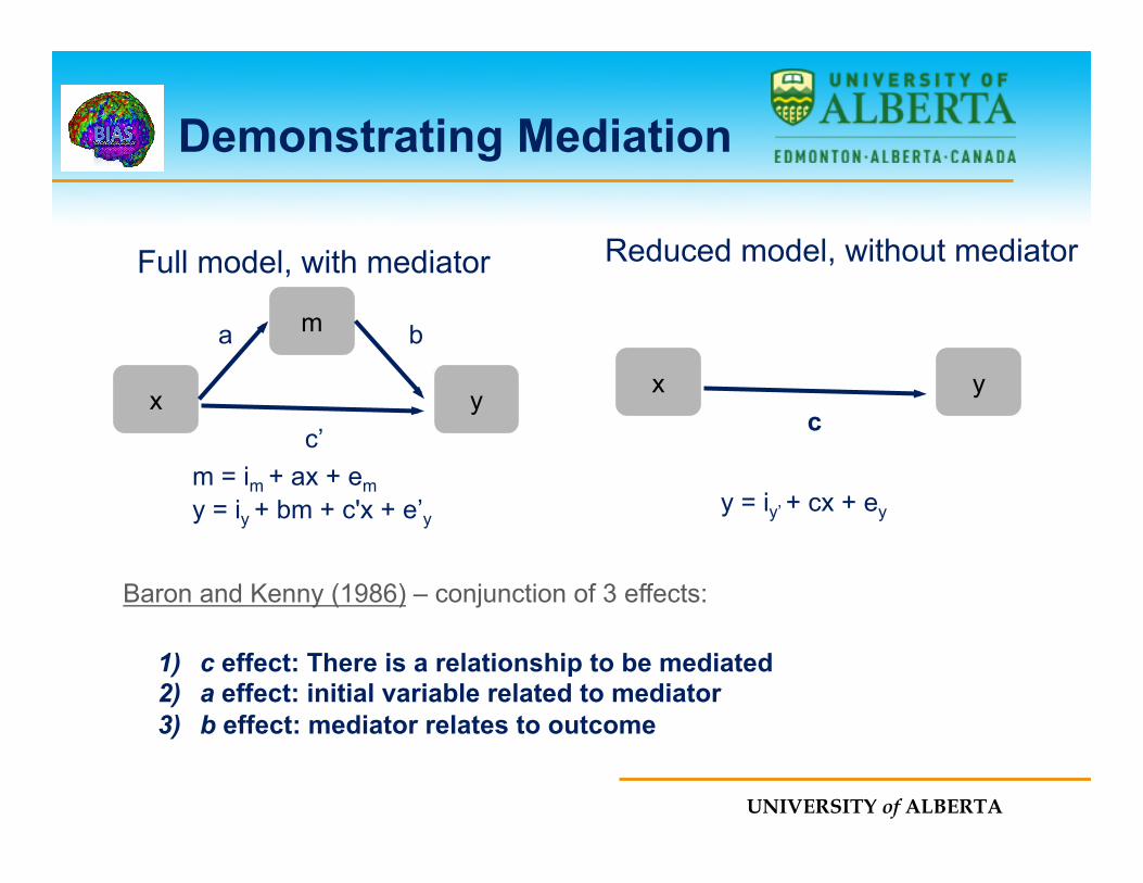
Demonstrating Mediation
x y
m a b
c’
x y c
Full model, with mediator Reduced model, without mediator
m = im + ax + em y = iy + bm + c'x + e’y y = iy’ + cx + ey
1) c effect: There is a relationship to be mediated 2) a effect: initial variable related to mediator 3) b effect: mediator relates to outcome
Baron and Kenny (1986) – conjunction of 3 effects:

UNIVERSITY of ALBERTA
Decomposition of Effects
Ø The mediation framework allows us to decompose the total effect of x on y as follows:
Ø Does m explain some of the x-y relationship?
² Test c – c’, which is equivalent to significance of a*b product.
c = c' + ab Total effect = Direct effect + Mediated effect
UNIVERSITY of ALBERTA
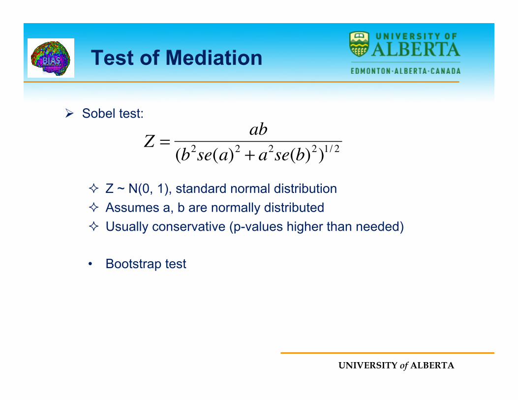
Test of Mediation
Ø Sobel test:
² Z ~ N(0, 1), standard normal distribution ² Assumes a, b are normally distributed ² Usually conservative (p-values higher than needed)
• Bootstrap test
�
Z =ab
(b2se(a)2 + a2se(b)2)1/ 2
UNIVERSITY of ALBERTA
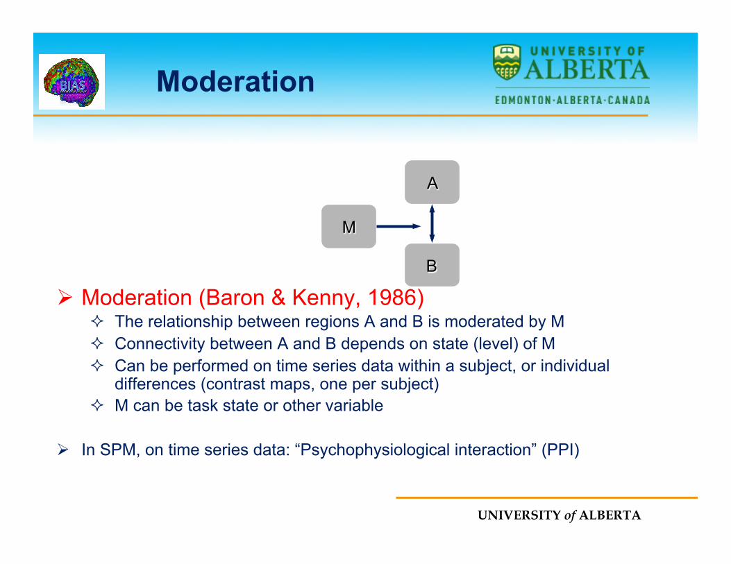
Moderation
Ø Moderation (Baron & Kenny, 1986) ² The relationship between regions A and B is moderated by M ² Connectivity between A and B depends on state (level) of M ² Can be performed on time series data within a subject, or individual
differences (contrast maps, one per subject) ² M can be task state or other variable
Ø In SPM, on time series data: “Psychophysiological interaction” (PPI)
M
B
A
UNIVERSITY of ALBERTA
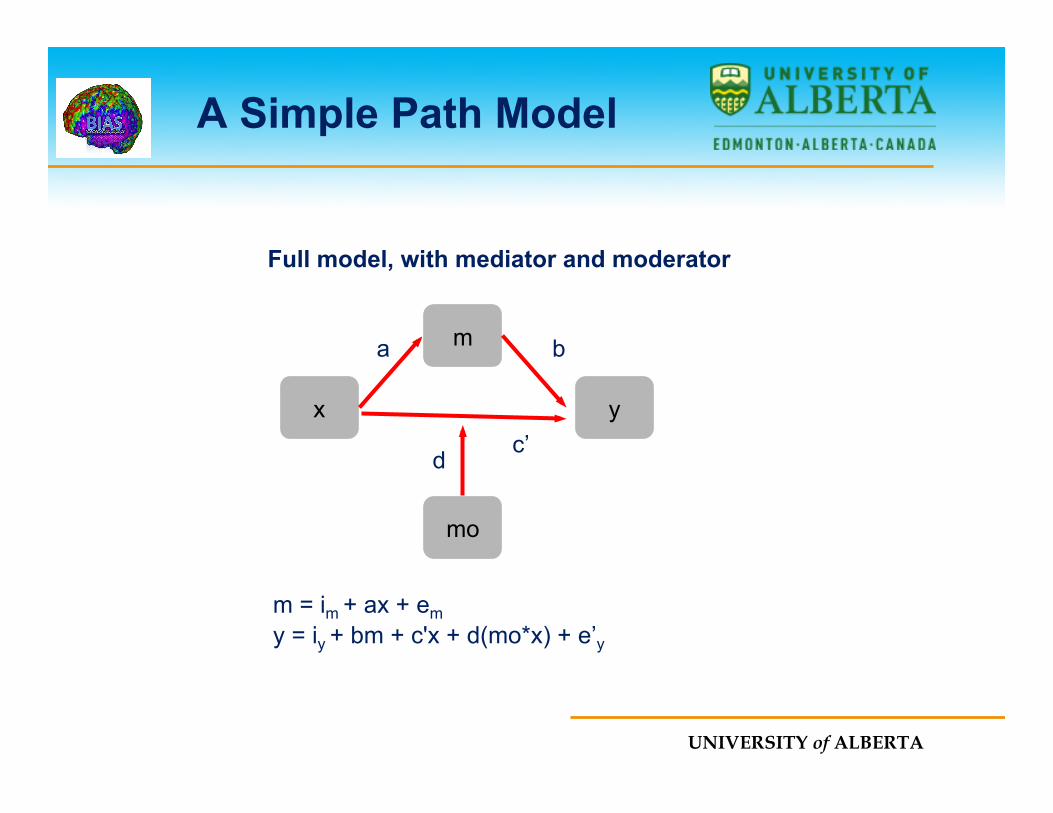
A Simple Path Model
x y
m a b
c’
Full model, with mediator and moderator
m = im + ax + em y = iy + bm + c'x + d(mo*x) + e’y
mo
d
UNIVERSITY of ALBERTA
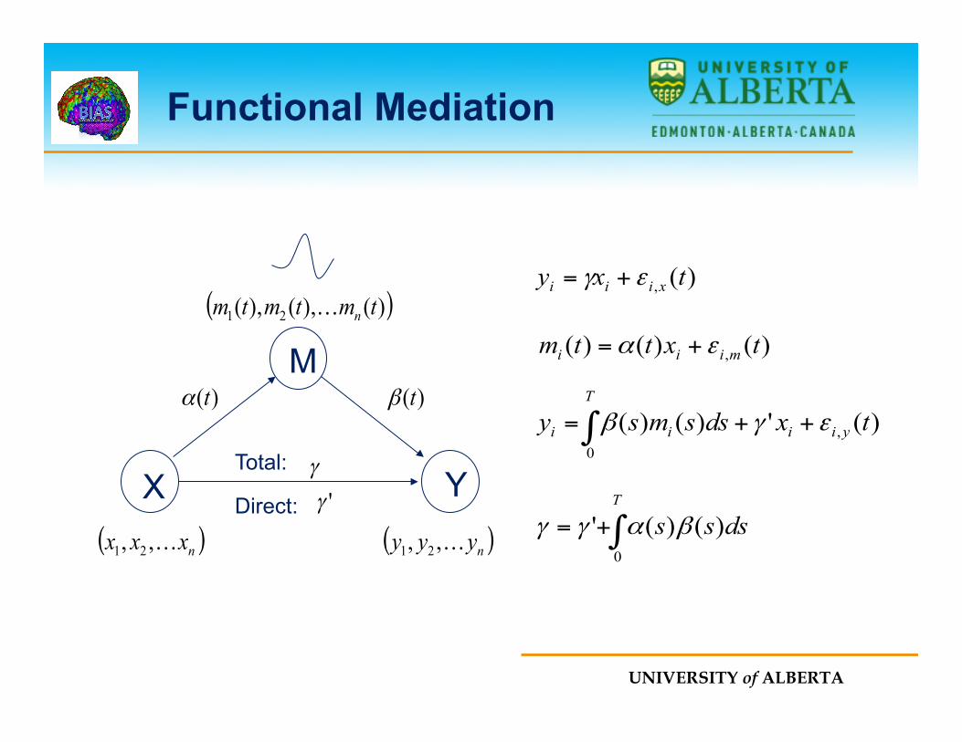
Functional Mediation
X
M
Y ( )nxxx …,, 21 ( )nyyy …,, 21
( ))(),(),( 21 tmtmtm n…
)(tα )(tβ
Total:
Direct: 'γγ
)()()( , txttm miii εα +=
)(')()( ,0
txdssmsy yii
T
ii εγβ ++= ∫
)(, txy xiii εγ +=
∫+=T
dsss0
)()(' βαγγ
UNIVERSITY of ALBERTA
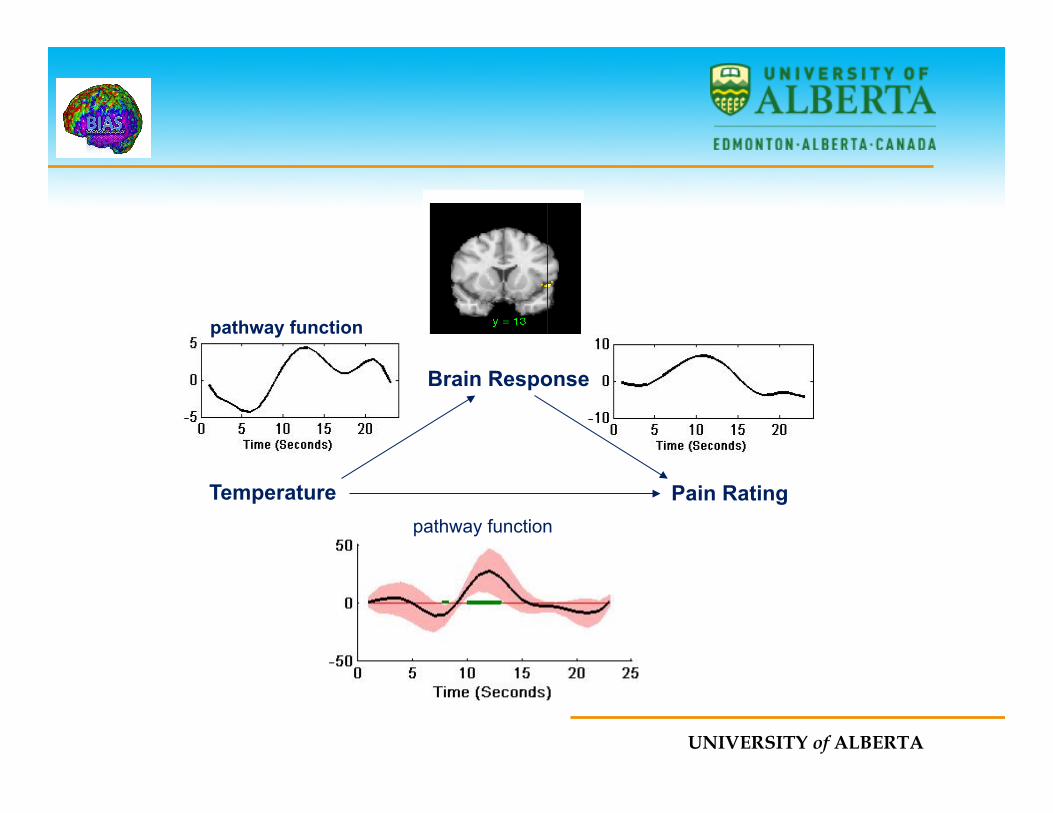
Temperature Pain Rating
Brain Response
pathway function
α pathway function β pathway function
UNIVERSITY of ALBERTA
Multivariate Methods
Ø We often use multivariate methods to study functional connectivity.
Ø When using multivariate methods observations at each voxel are considered jointly.
Ø This has the potential to allow for better understanding of how different brain regions interact with one another.
UNIVERSITY of ALBERTA
Principal Components Analysis
Ø Principal components analysis involves finding spatial modes, or eigenimages, in the data.
Ø Spatial modes are the patterns that account for most of the variance-covariance structure in the data.
Ø The eigenimages are obtained using singular value decomposition (SVD), which decomposes the data into two sets of orthogonal vectors that correspond to patterns in space and time.
UNIVERSITY of ALBERTA
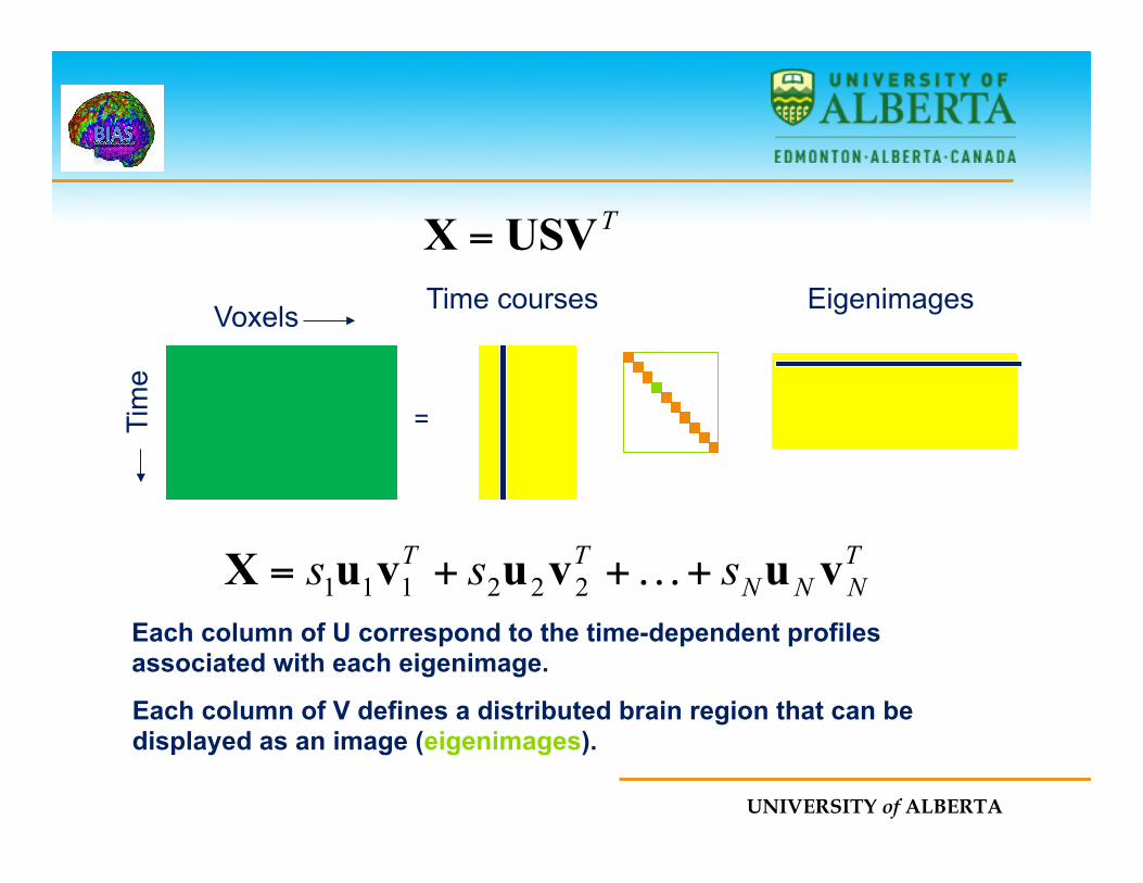
TUSVX =
Voxels
Tim
e
=
Eigenimages Time courses
TNNN
TT sss vuvuvuX +++= …222111
Each column of V defines a distributed brain region that can be displayed as an image (eigenimages).
Each column of U correspond to the time-dependent profiles associated with each eigenimage.
UNIVERSITY of ALBERTA Worsley
UNIVERSITY of ALBERTA
Independent Components Analysis
Ø Independent Components Analysis (ICA) is a family of techniques used to extract independent signals from some source signal.
Ø ICA provides a method to blindly separate the data into spatially independent components.
Ø The key assumption is that the data set consists of p spatially independent components, which are linearly mixed and spatially fixed.
UNIVERSITY of ALBERTA
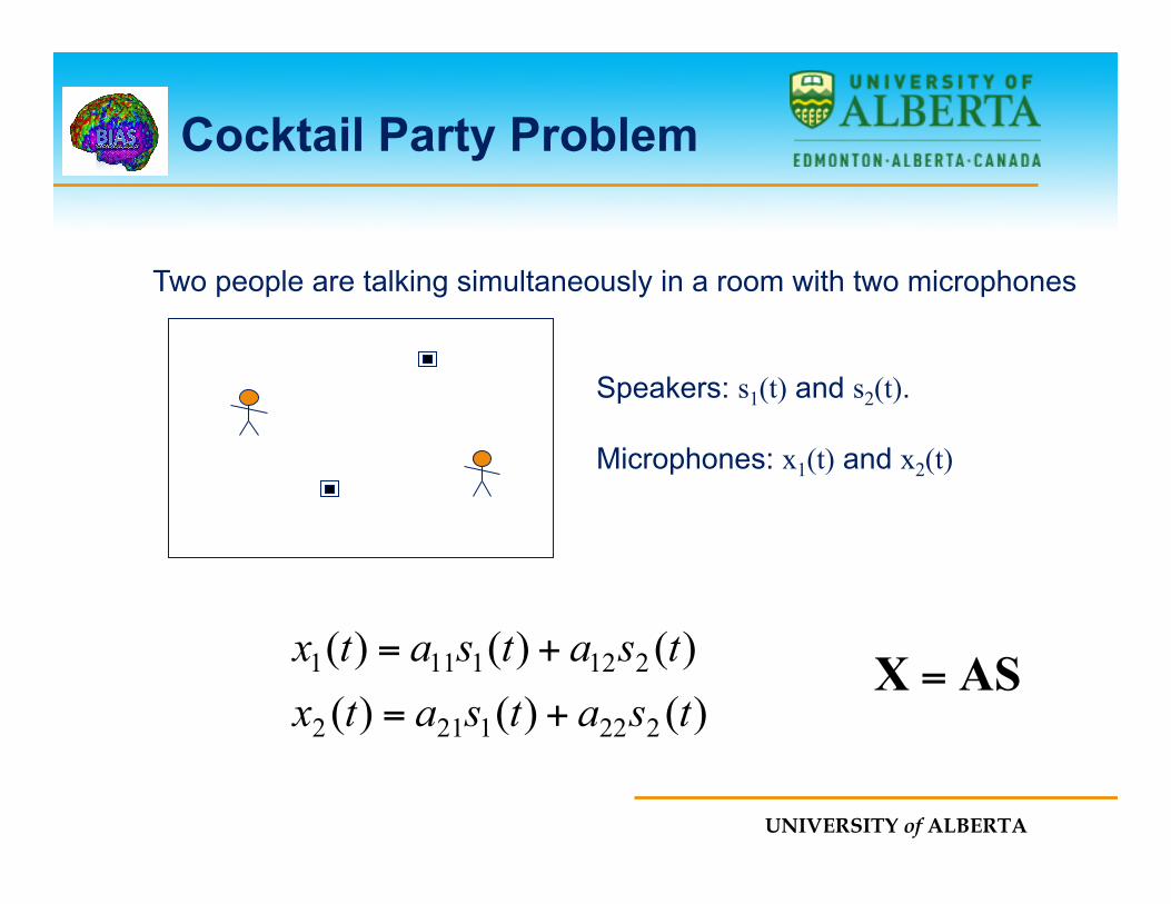
Two people are talking simultaneously in a room with two microphones.
Cocktail Party Problem
Speakers: s1(t) and s2(t). Microphones: x1(t) and x2(t)
)()()()()()(
2221212
2121111
tsatsatxtsatsatx
+=
+= ASX =
UNIVERSITY of ALBERTA
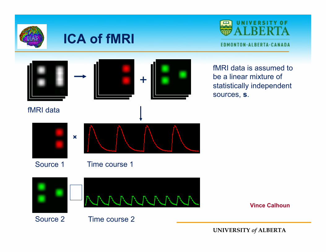
ICA of fMRI
+
A[ ]1 2Ts s=s
fMRI data
fMRI data is assumed to be a linear mixture of statistically independent sources, s.
×
×
Source 1
Source 2
Time course 1
Time course 2
Vince Calhoun
×
×

UNIVERSITY of ALBERTA
ASX =
Problem Formulation
Ø We want to solve:
where A is the mixing matrix, S is the source matrix and X is the data matrix. Both A and S are unknown.
Ø Assume that Cov(X)=I and A is orthogonal.
Ø Find A such that S=ATX.
UNIVERSITY of ALBERTA
Assumptions
Ø ICA is able the solve this problem by exploiting some key assumptions.
Ø Assumptions:
² Linear mixing of sources.
² The components si are statistically independent.
² The components si are non-Gaussian.
UNIVERSITY of ALBERTA
Mutual Information
Ø One approach is to minimize the mutual information between different components.
Ø This is equivalent to minimizing the Kullback-Leibler divergence between the joint density and the product of the marginal densities.
Ø The Kullback-Leibler divergence is a measure of similarity between two density functions.
UNIVERSITY of ALBERTA
ICA for fMRI
Ø It is assumed that the fMRI data can be modeled by identifying sets of voxels whose activity both vary together over time and are maximally different from the activity in other sets.
Ø Decompose the data set into a set of spatially independent component maps with a set of corresponding time-courses.
UNIVERSITY of ALBERTA
Voxels
Tim
e
=
Mixing Matrix
Components Data
Spatially independent Components
Time Courses
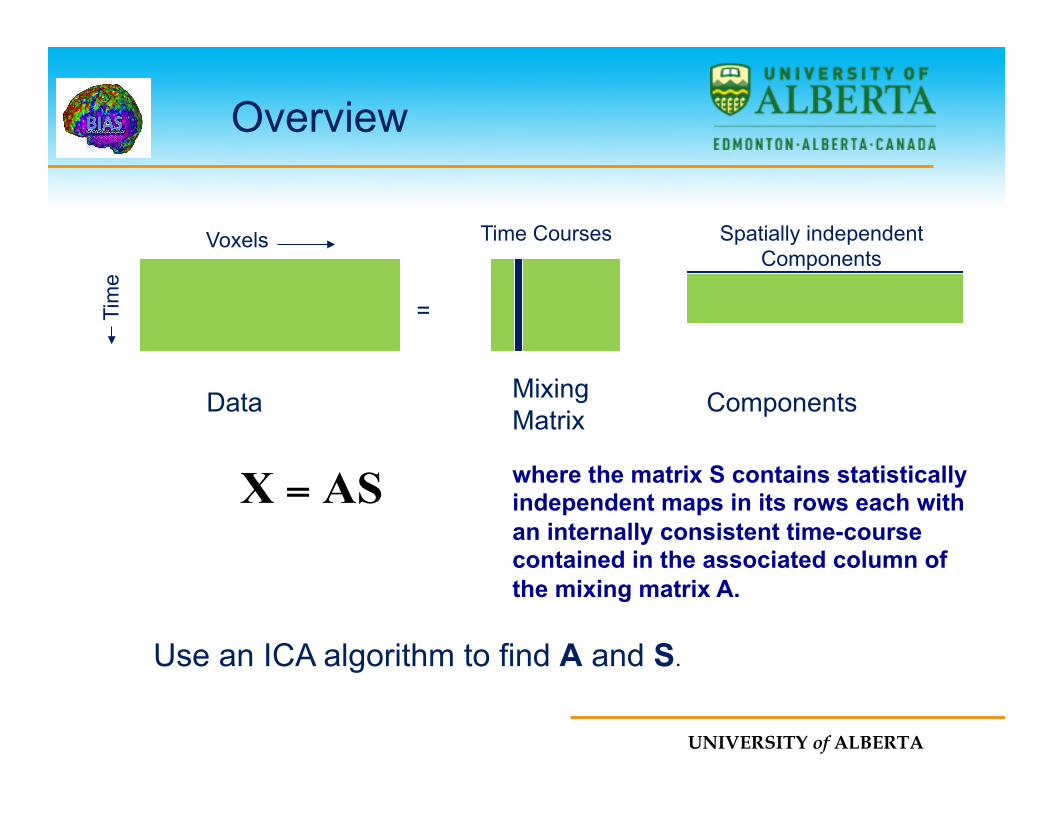
ASX =
Use an ICA algorithm to find A and S.
Overview
where the matrix S contains statistically independent maps in its rows each with an internally consistent time-course contained in the associated column of the mixing matrix A.
UNIVERSITY of ALBERTA
Comments
Ø Unlike PCA which assumes an orthonormality constraint, ICA assumes statistical independence among a collection of spatial patterns.
Ø Independence is a stronger requirement than orthonormality.
Ø However, in ICA the spatially independent components are not ranked in order of importance as they are when performing PCA.
UNIVERSITY of ALBERTA
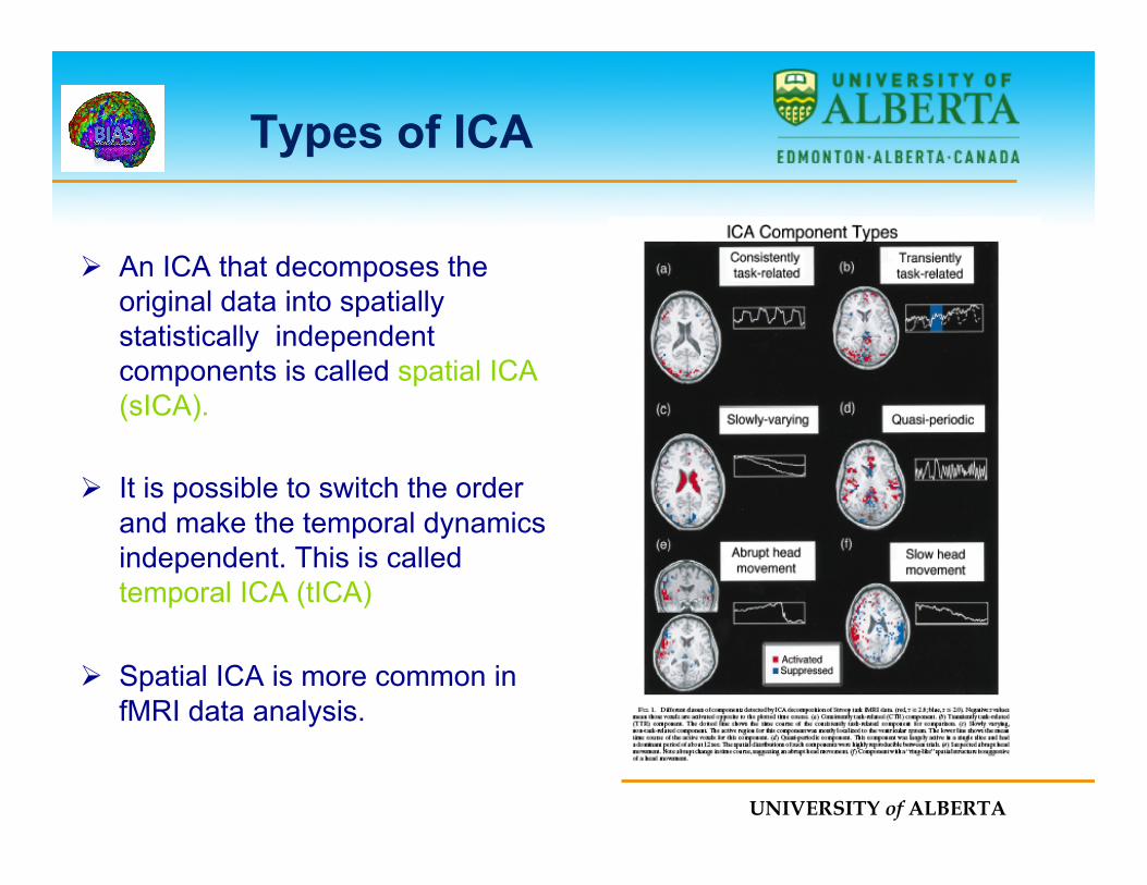
Types of ICA
Ø An ICA that decomposes the original data into spatially statistically independent components is called spatial ICA (sICA).
Ø It is possible to switch the order and make the temporal dynamics independent. This is called temporal ICA (tICA)
Ø Spatial ICA is more common in fMRI data analysis.
UNIVERSITY of ALBERTA
Multi-subject Analysis
Ø Using ICA to analyze fMRI data from multiple subjects raises several questions.
² How should components be combined across subjects? ² How should the final results be thresholded and/or presented?
Ø There are several approaches:
² Stack time courses (forces time courses to be the same) ² Stack images and back-reconstruct (allows time courses to vary,
allows some flexibility in images) ² Stack into a cube (forces images and time courses to be the same)
UNIVERSITY of ALBERTA
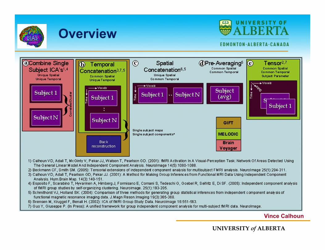
Overview
Vince Calhoun
UNIVERSITY of ALBERTA
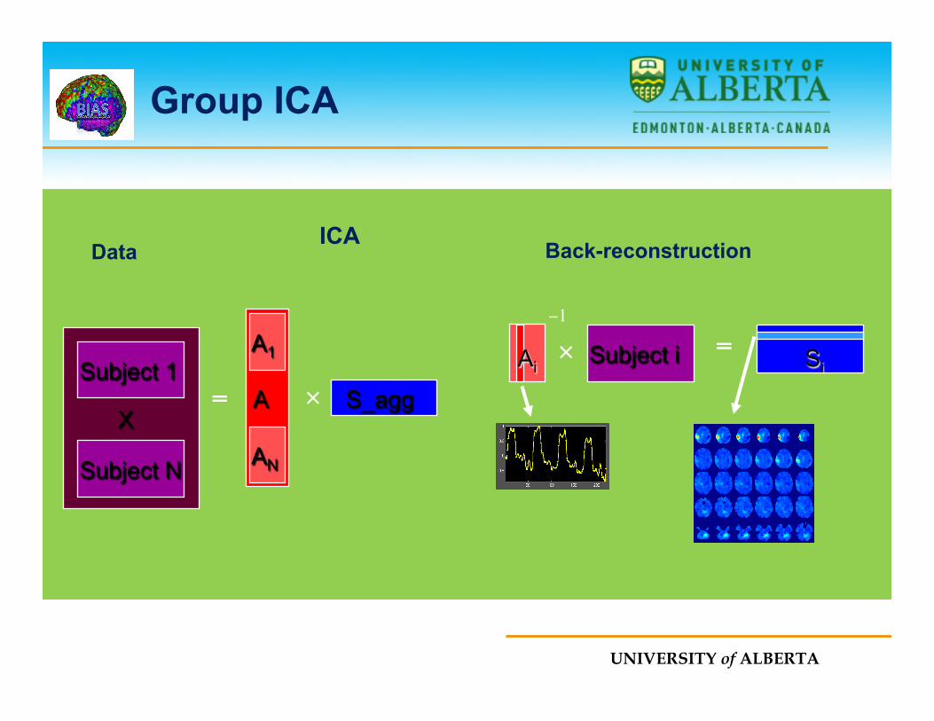
Group ICA
Ø Group ICA is based on temporal concatenation.
Ø It decomposes the group matrix, and estimates through back-reconstruction the spatial weights for each subject for a component of interest.
Ø For each subject the spatial weights at each voxel are treated as random variables, and a one-sample t-test is used to test whether that voxel loaded significantly on that component in the group.
UNIVERSITY of ALBERTA
Group ICA
X
Subject 1
Subject N
Data
A S_agg
ICA
A1
AN
= ×
Subject i
Back-reconstruction
×1−
=Ai Si
UNIVERSITY of ALBERTA
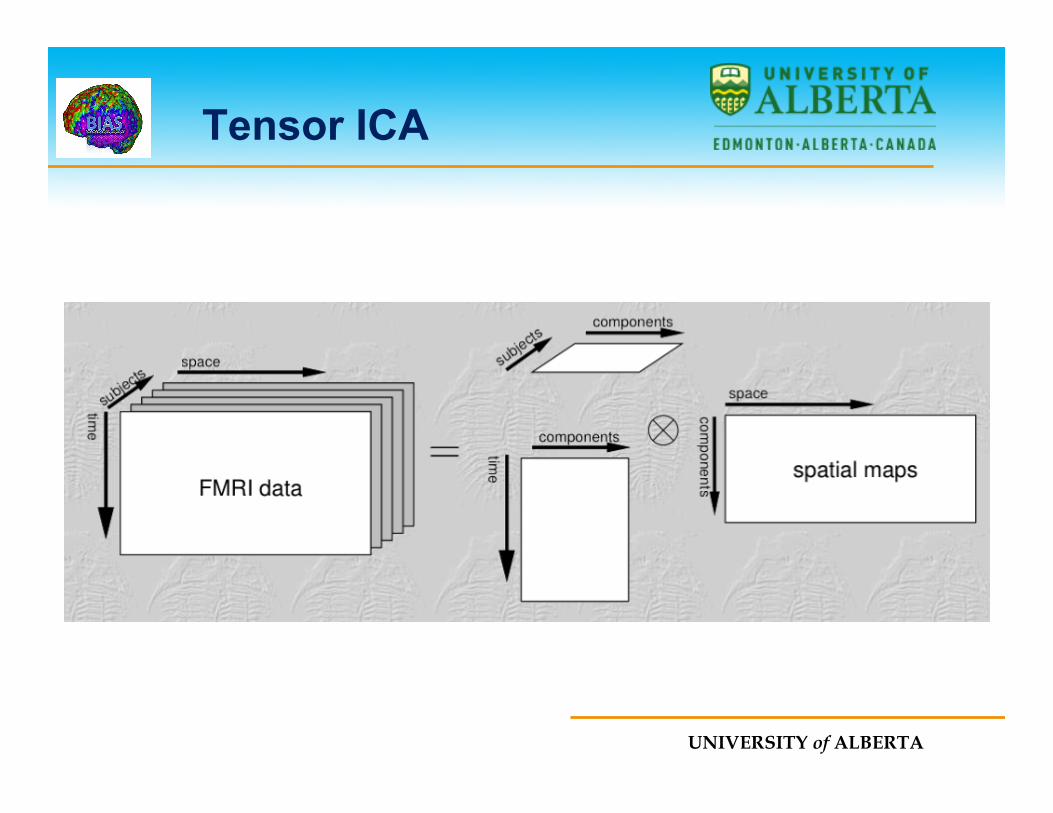
Tensor ICA
Ø Tensor ICA decomposes a three-way data set into a set of independent spatial maps together with associated time courses and subject modes.
Ø This allows us to characterize the signal variation across the temporal, spatial and subject/session domain for each component.
UNIVERSITY of ALBERTA
Tensor ICA

UNIVERSITY of ALBERTA
Effective Connectivity
UNIVERSITY of ALBERTA
Effective Connectivity
Ø Effective connectivity is the influence one neuronal system exerts over another.
Ø Effective connectivity depends on two models:
² A neuroanatomical model that describes which areas are connected.
² A mathematical model that describes how areas are connected.
UNIVERSITY of ALBERTA
Structural Equation Modelling
Ø Structural equation Modeling (SEM) was first applied to imaging data by McIntosh and Gonzalez-Lima (1991).
Ø SEM allows for the analysis of more complicated models consisting of many different ROIs.
Ø Instead of considering variables individually the emphasis in SEM lies on the variance-covariance structure of the data.
UNIVERSITY of ALBERTA
SEM
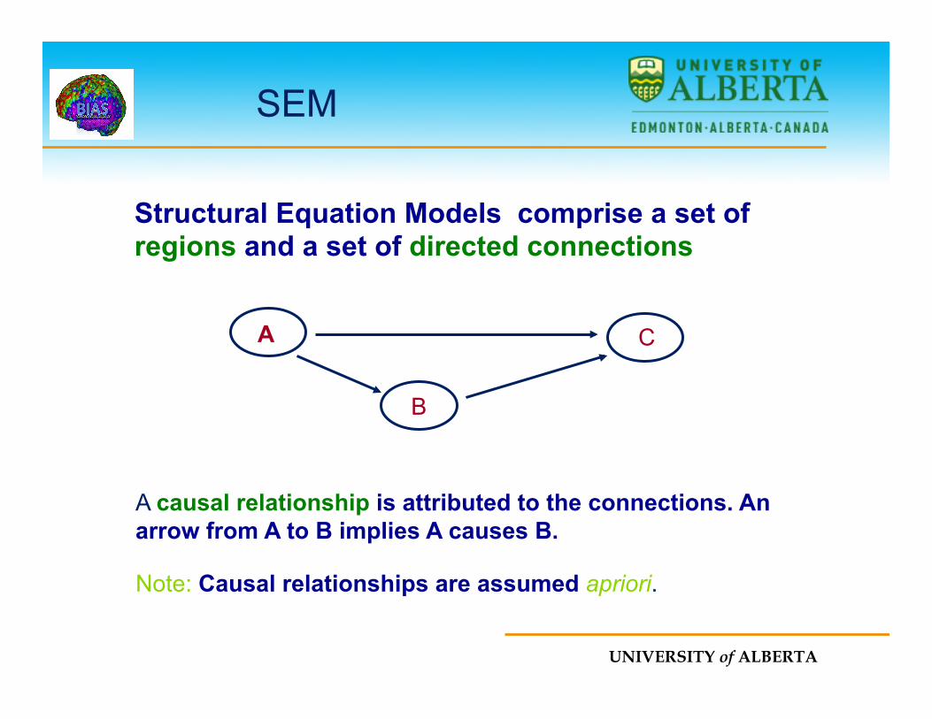
Structural Equation Models comprise a set of regions and a set of directed connections.
A causal relationship is attributed to the connections. An arrow from A to B implies A causes B.
Note: Causal relationships are assumed apriori.
A C
B
UNIVERSITY of ALBERTA
SEM
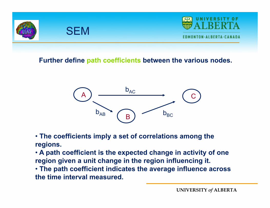
• The coefficients imply a set of correlations among the regions. • A path coefficient is the expected change in activity of one region given a unit change in the region influencing it. • The path coefficient indicates the average influence across the time interval measured.
A C
B
Further define path coefficients between the various nodes.
bAC
bAB bBC
UNIVERSITY of ALBERTA
SEM
Ø The covariance of the data represents how the activities in two or more regions are related.
Ø In SEM we seek to minimize the difference between the observed covariance matrix and the one implied by the structure of the model.
Ø The parameters of the model are adjusted to minimize the difference between the observed and modeled covariance matrix.
UNIVERSITY of ALBERTA
Set-Up
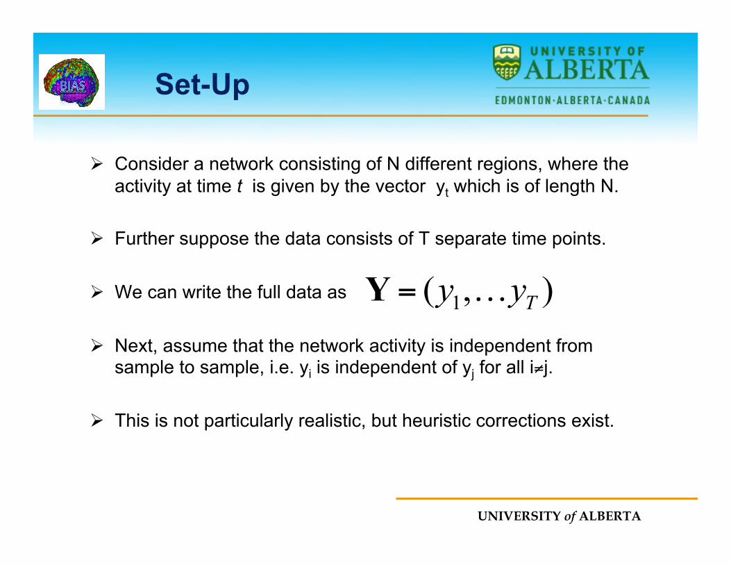
Ø Consider a network consisting of N different regions, where the activity at time t is given by the vector yt which is of length N.
Ø Further suppose the data consists of T separate time points.
Ø We can write the full data as
Ø Next, assume that the network activity is independent from sample to sample, i.e. yi is independent of yj for all i≠j.
Ø This is not particularly realistic, but heuristic corrections exist.
),( 1 Tyy …=Y
UNIVERSITY of ALBERTA
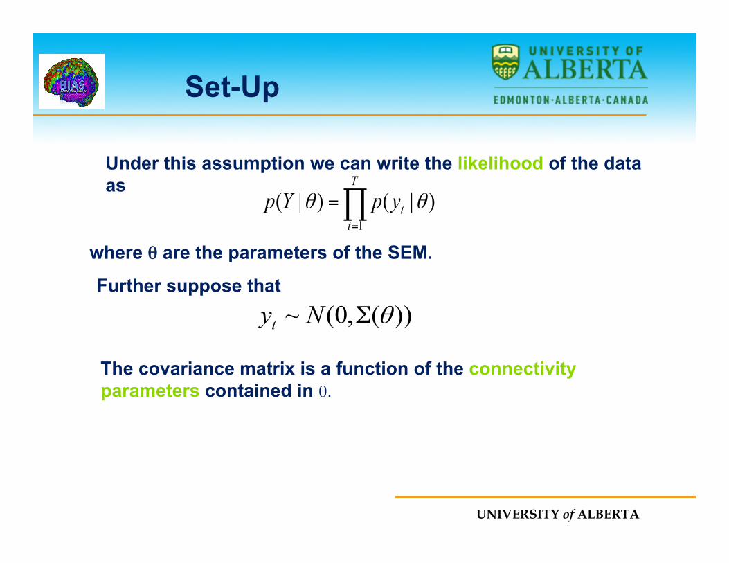
))(,0(~ θΣNyt
The covariance matrix is a function of the connectivity parameters contained in θ.
Further suppose that
∏=
=T
ttypYp
1
)|()|( θθ
Under this assumption we can write the likelihood of the data as
where θ are the parameters of the SEM.
Set-Up
UNIVERSITY of ALBERTA
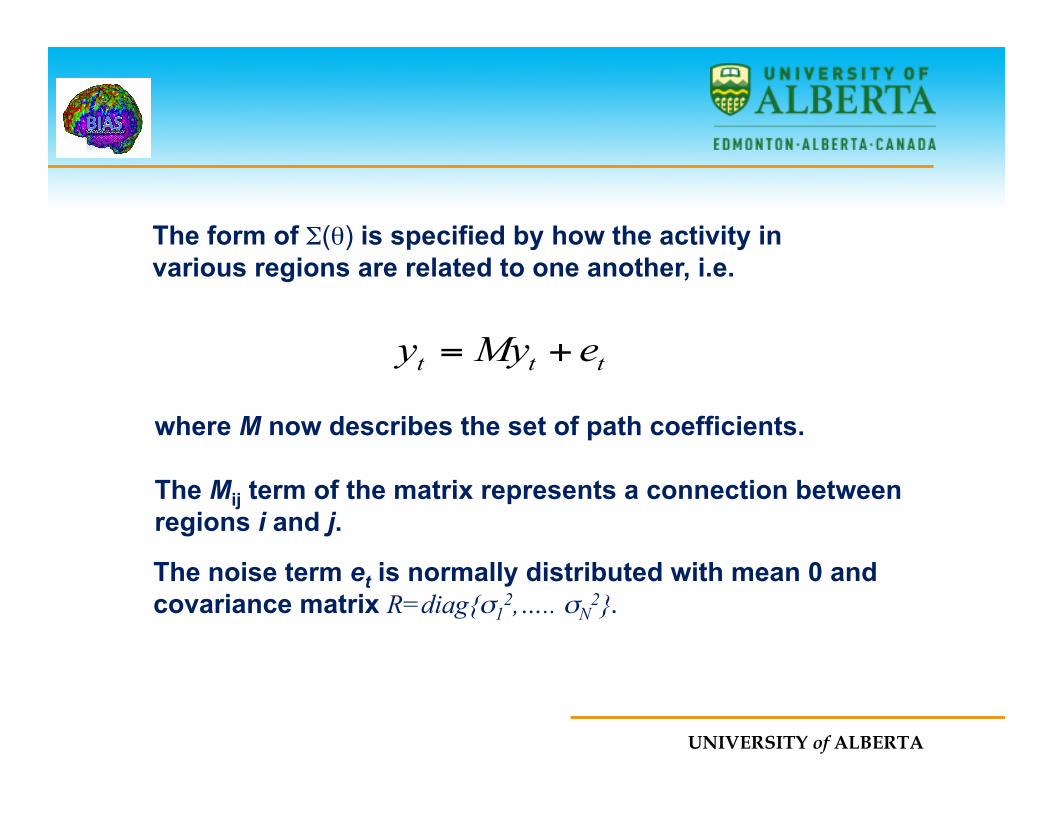
The form of Σ(θ) is specified by how the activity in various regions are related to one another, i.e.
where M now describes the set of path coefficients. The Mij term of the matrix represents a connection between regions i and j.
ttt eMyy +=
The noise term et is normally distributed with mean 0 and covariance matrix R=diag{σ1
2,….. σN2}.
UNIVERSITY of ALBERTA
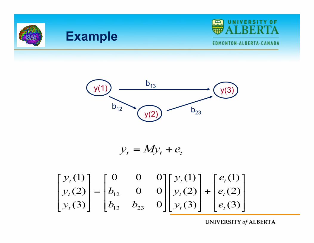
y(1) b13
b12 b23 y(2)
y(3)
ttt eMyy +=
⎥⎥⎥
⎦
⎤
⎢⎢⎢
⎣
⎡
+
⎥⎥⎥
⎦
⎤
⎢⎢⎢
⎣
⎡
⎥⎥⎥
⎦
⎤
⎢⎢⎢
⎣
⎡
=
⎥⎥⎥
⎦
⎤
⎢⎢⎢
⎣
⎡
)3()2()1(
)3()2()1(
000000
)3()2()1(
2313
12
t
t
t
t
t
t
t
t
t
eee
yyy
bbb
yyy
Example

UNIVERSITY of ALBERTA
We can rewrite yt as
The parameters θ are the unknown elements of the matrices M and R.
tt eMIy 1)( −−=Hence, we can write the covariance matrix of yt as
( ) ( )TMIRMI 11 )()( −− −−=Σ θ
))(,0(~ θΣNytThis gives us the desired path coefficients.
Find the parameters θ that maximize the likelihood function:
UNIVERSITY of ALBERTA
Inference
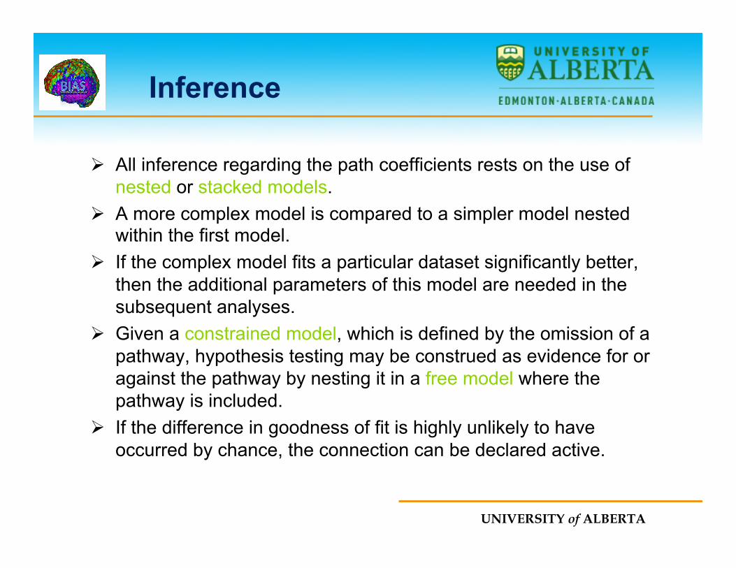
Ø All inference regarding the path coefficients rests on the use of nested or stacked models.
Ø A more complex model is compared to a simpler model nested within the first model.
Ø If the complex model fits a particular dataset significantly better, then the additional parameters of this model are needed in the subsequent analyses.
Ø Given a constrained model, which is defined by the omission of a pathway, hypothesis testing may be construed as evidence for or against the pathway by nesting it in a free model where the pathway is included.
Ø If the difference in goodness of fit is highly unlikely to have occurred by chance, the connection can be declared active.
UNIVERSITY of ALBERTA
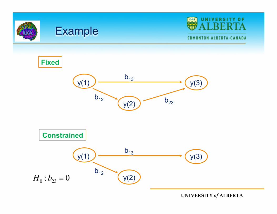
y(1) b13
b12 b23 y(2)
y(3)
y(1) b13
b12 y(2)
y(3)
Example
Fixed
Constrained
0: 230 =bH
UNIVERSITY of ALBERTA
Likelihood Ratio Test
Ø The likelihood ratio test (LRT) is a statistical test of the goodness-of-fit between two models.
Ø A relatively more complex model is compared to a simpler model to determine whether it fits the dataset significantly better.
Ø If so, the additional parameters in the more complex model need to be included.
UNIVERSITY of ALBERTA
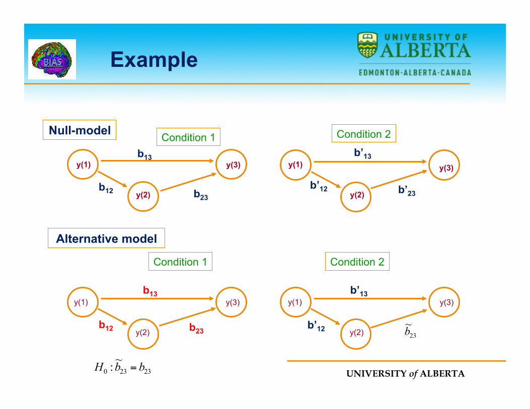
Comparing Conditions
Ø We can take a similar approach to making inference about changes in effective connectivity between different experiment conditions.
Ø First partition the data according to the different experimental conditions.
Ø Next create a null-model where path coefficients are constrained to be equal between conditions and an alternative model where certain coefficients of interest are allowed to vary.
UNIVERSITY of ALBERTA
y(1) b13
b12 b23 y(2)
y(3)
Example
Null-model
Alternative model
y(1) b’13
b’12 b’23 y(2)
y(3)
y(1) b13
b12 b23 y(2)
y(3) y(1) b’13
b’12 y(2)
y(3)
23~b
Condition 1 Condition 2
Condition 1 Condition 2
23230~: bbH =
UNIVERSITY of ALBERTA
Comparing Conditions
Ø Use the LRT to test whether there are significant differences between the models.
Ø If a significant difference exists we reject the hypothesis that the path coefficients are equal in both conditions.
Ø SEM discounts temporal information. Hence, permuted data sets produce the same path coefficients as the original data.
Ø We can compensate for temporal autocorrelation by using corrected degrees of freedom.
Ø However, models that include the temporal order of the data may be more appropriate.
UNIVERSITY of ALBERTA
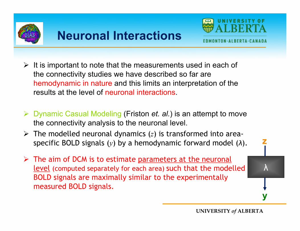
Neuronal Interactions
Ø It is important to note that the measurements used in each of the connectivity studies we have described so far are hemodynamic in nature and this limits an interpretation of the results at the level of neuronal interactions.
Ø Dynamic Casual Modeling (Friston et. al.) is an attempt to move the connectivity analysis to the neuronal level.
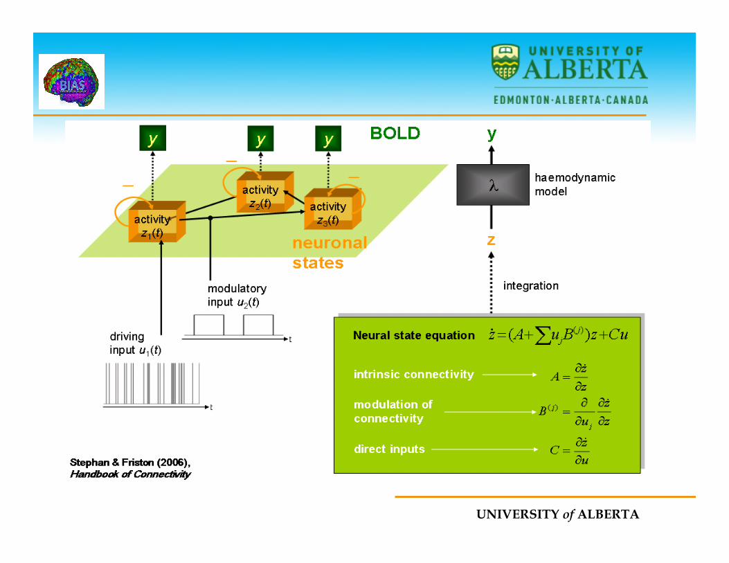
Ø The modelled neuronal dynamics (z) is transformed into area-specific BOLD signals (y) by a hemodynamic forward model (λ).
Ø The aim of DCM is to estimate parameters at the neuronal level (computed separately for each area) such that the modelled BOLD signals are maximally similar to the experimentally measured BOLD signals.
λ
z
y
UNIVERSITY of ALBERTA
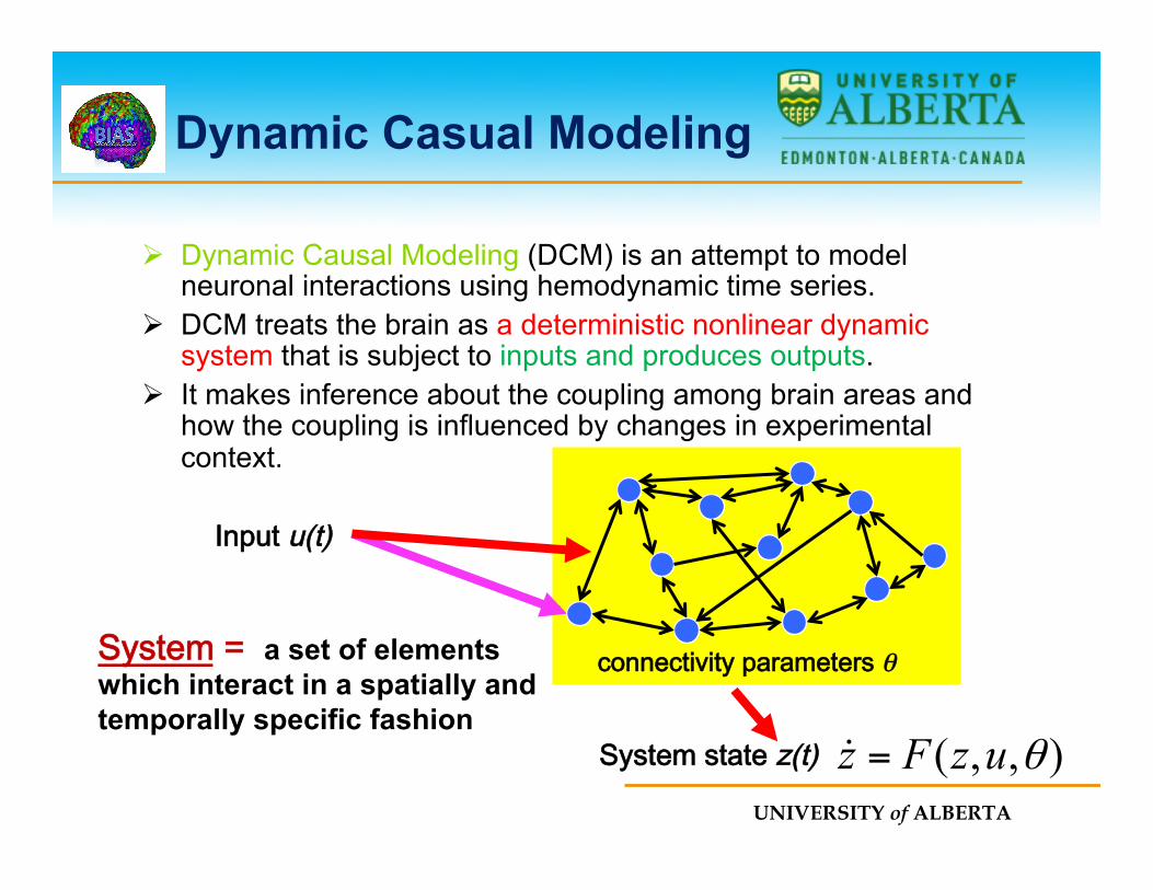
Dynamic Casual Modeling
Ø Dynamic Causal Modeling (DCM) is an attempt to model neuronal interactions using hemodynamic time series.
Ø DCM treats the brain as a deterministic nonlinear dynamic system that is subject to inputs and produces outputs.
Ø It makes inference about the coupling among brain areas and how the coupling is influenced by changes in experimental context.
Input u(t)
connectivity parameters θ
System state z(t)
System = a set of elements which interact in a spatially and temporally specific fashion
),,( θuzFz =!
UNIVERSITY of ALBERTA
Ø DCM is based on a neuronal model of interacting cortical regions, supplemented with a forward model of how neuronal activity is transformed into a measured response.
Ø Effective connectivity is parameterized in terms of the coupling among unobserved neuronal activity in different regions.
Ø We can estimate these parameters by perturbing the system and measuring the response.
UNIVERSITY of ALBERTA
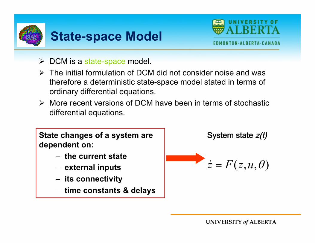
State-space Model
Ø DCM is a state-space model. Ø The initial formulation of DCM did not consider noise and was
therefore a deterministic state-space model stated in terms of ordinary differential equations.
Ø More recent versions of DCM have been in terms of stochastic differential equations.
System state z(t) State changes of a system are dependent on:
– the current state – external inputs – its connectivity – time constants & delays
),,( θuzFz =!
UNIVERSITY of ALBERTA
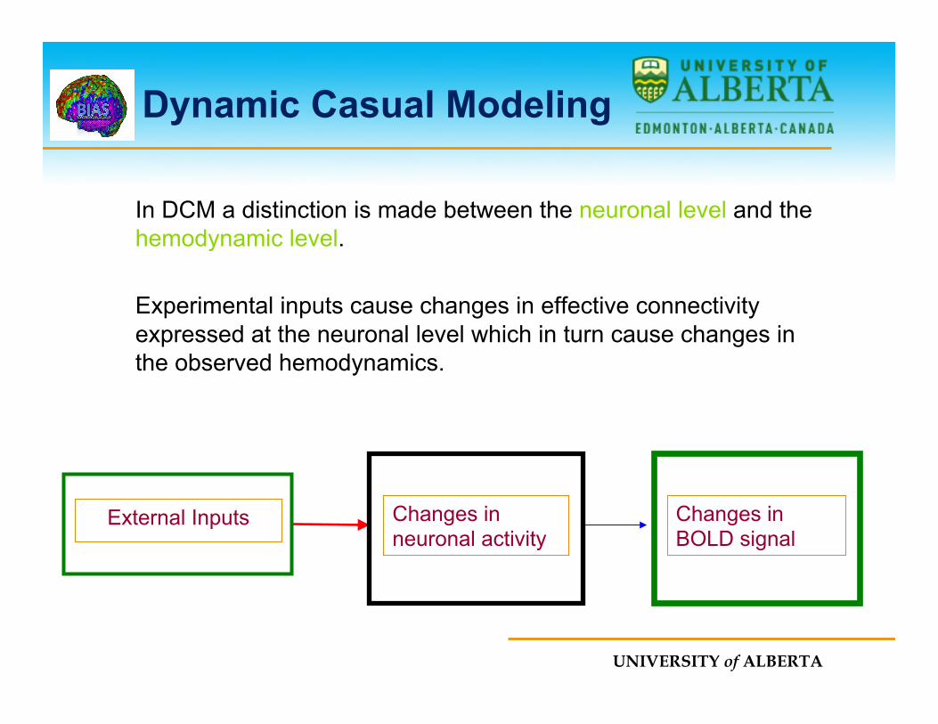
Dynamic Casual Modeling
In DCM a distinction is made between the neuronal level and the hemodynamic level. Experimental inputs cause changes in effective connectivity expressed at the neuronal level which in turn cause changes in the observed hemodynamics.
External Inputs Changes in neuronal activity
Changes in BOLD signal

UNIVERSITY of ALBERTA
Dynamic Casual Modeling
Ø DCM uses a bilinear model for the neuronal level and an extended Balloon model for the hemodynamic level.
Ø In a DCM model we have J experimental inputs and N outputs (one for each region).
Ø Each region has five state variables, four corresponding to the hemodynamic model and a fifth corresponding to neuronal activity.
UNIVERSITY of ALBERTA
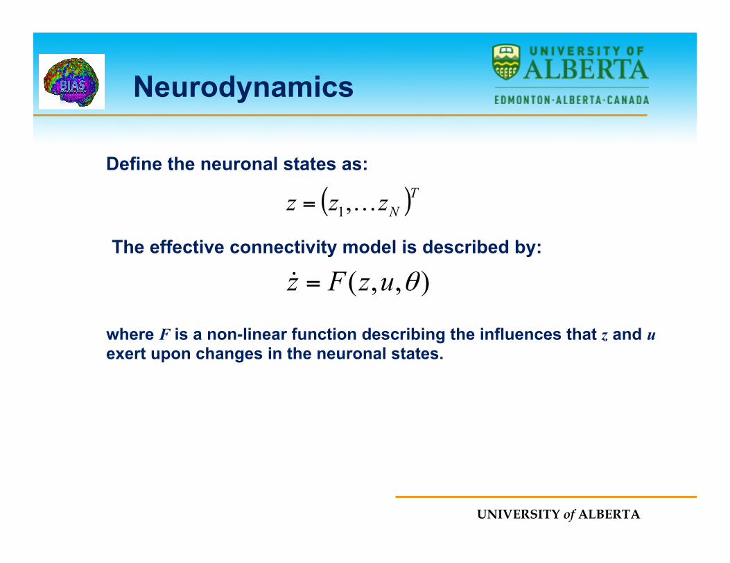
Neurodynamics
( )TNzzz …,1=
),,( θuzFz =!
where F is a non-linear function describing the influences that z and u exert upon changes in the neuronal states.
Define the neuronal states as:
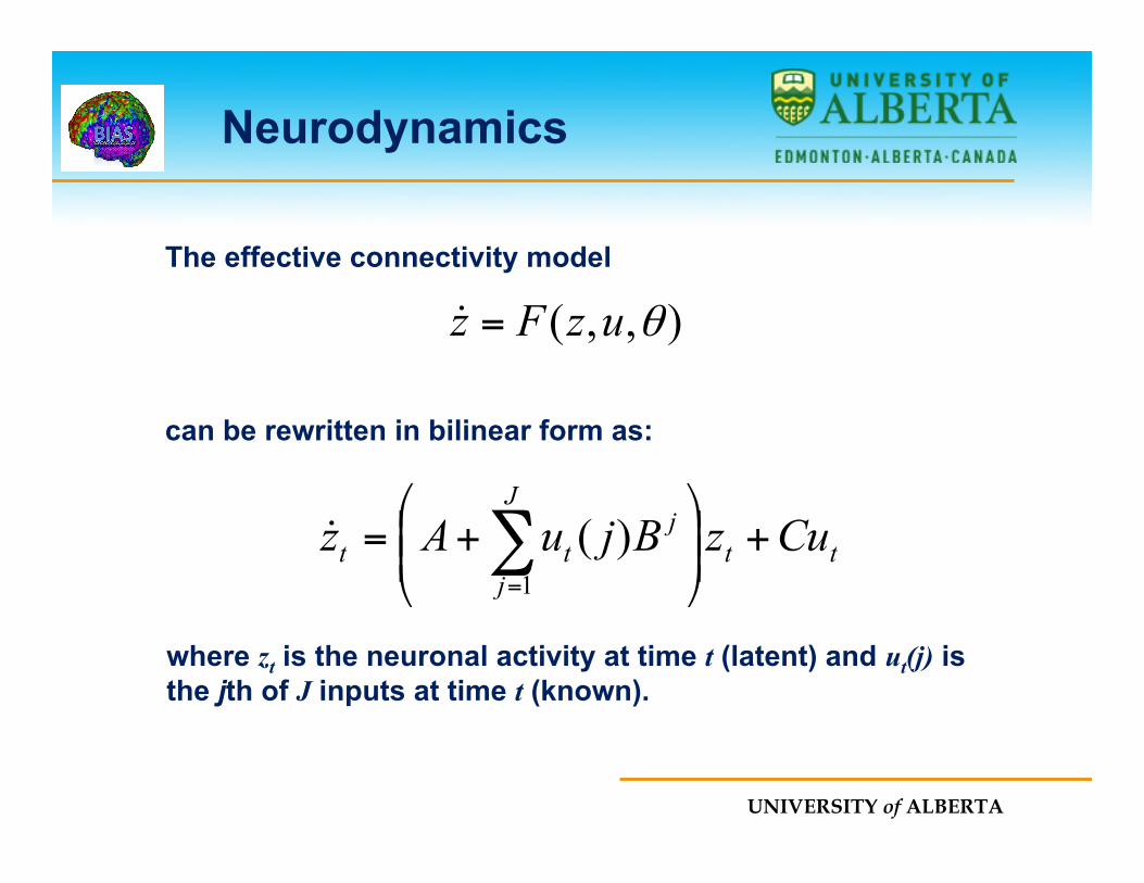
The effective connectivity model is described by:

UNIVERSITY of ALBERTA
Bilinear form
ufc∂
∂=
uxfb∂∂
∂=
2
cubxuaxuxf ++≈),(
The model consists of a bivariate nonlinear function. We can approximate such a function using a bilinear approximation:
xfa∂
∂=
where
UNIVERSITY of ALBERTA
Neurodynamics
tt
J
j
jtt CuzBjuAz +⎟⎟
⎠
⎞⎜⎜⎝
⎛+= ∑
=1)(!
where zt is the neuronal activity at time t (latent) and ut(j) is the jth of J inputs at time t (known).
The effective connectivity model can be rewritten in bilinear form as:
),,( θuzFz =!
UNIVERSITY of ALBERTA
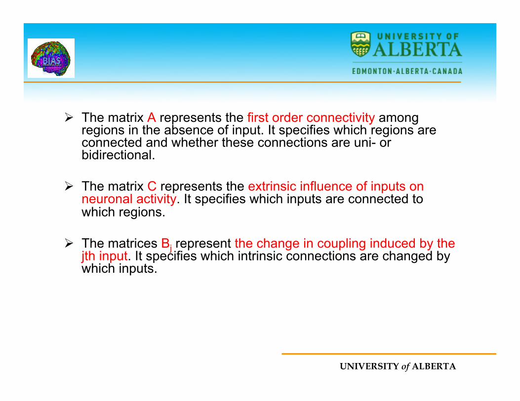
Ø The matrix A represents the first order connectivity among regions in the absence of input. It specifies which regions are connected and whether these connections are uni- or bidirectional.
Ø The matrix C represents the extrinsic influence of inputs on neuronal activity. It specifies which inputs are connected to which regions.
Ø The matrices Bj represent the change in coupling induced by the jth input. It specifies which intrinsic connections are changed by which inputs.
UNIVERSITY of ALBERTA
Interpretation
Ø The units of connection are per unit time and therefore correspond to rates.
Ø A strong connection means an influence that is expressed quickly or with a small time constant.
UNIVERSITY of ALBERTA
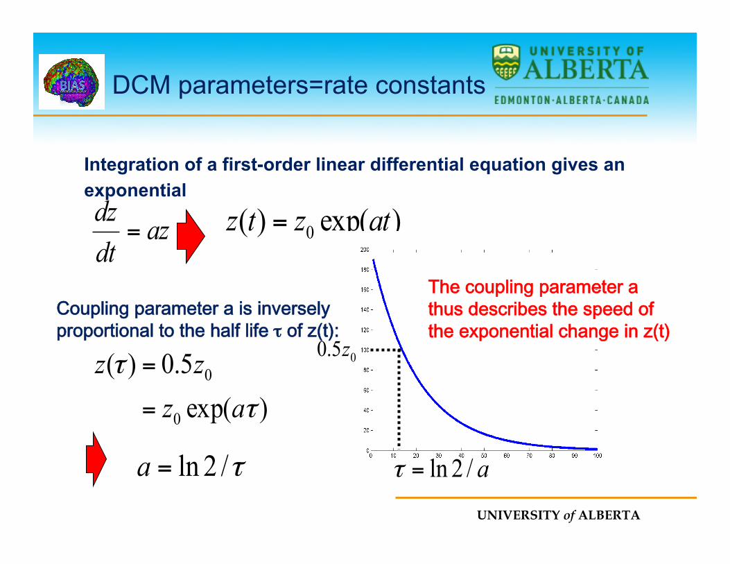
DCM parameters=rate constants
azdtdz
= )exp()( 0 atztz =
The coupling parameter a thus describes the speed ofthe exponential change in z(t)
)exp(5.0)(
0
0
τ
τ
azzz
=
=
Integration of a first-order linear differential equation gives an exponential function:
τ/2ln=a
05.0 z
a/2ln=τ
Coupling parameter a is inverselyproportional to the half life τ of z(t):
UNIVERSITY of ALBERTA
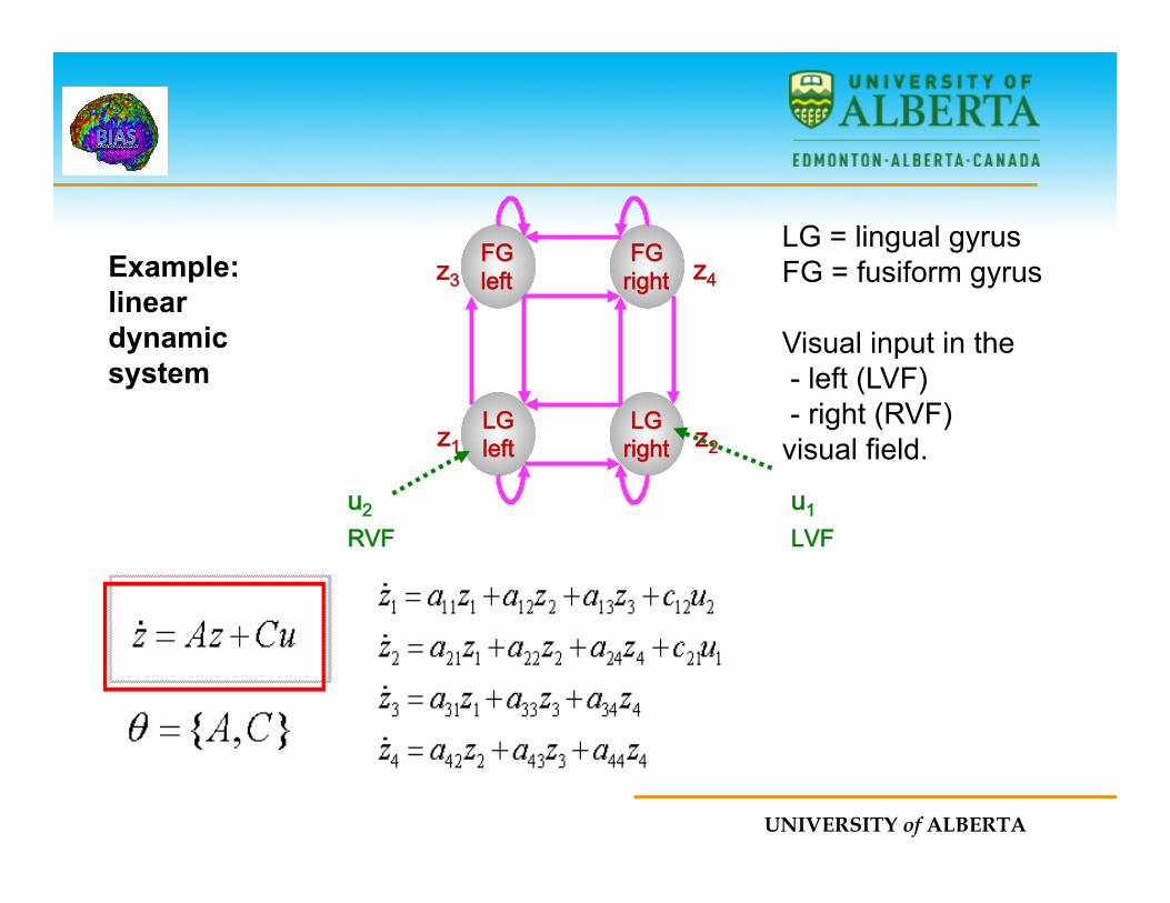
Example: linear dynamic system
LG left
LG right
FG right
FG left
LG = lingual gyrus FG = fusiform gyrus Visual input in the - left (LVF) - right (RVF) visual field. z1 z2
z4 z3
RVF LVF
u2 RVF
u1 LVF
UNIVERSITY of ALBERTA
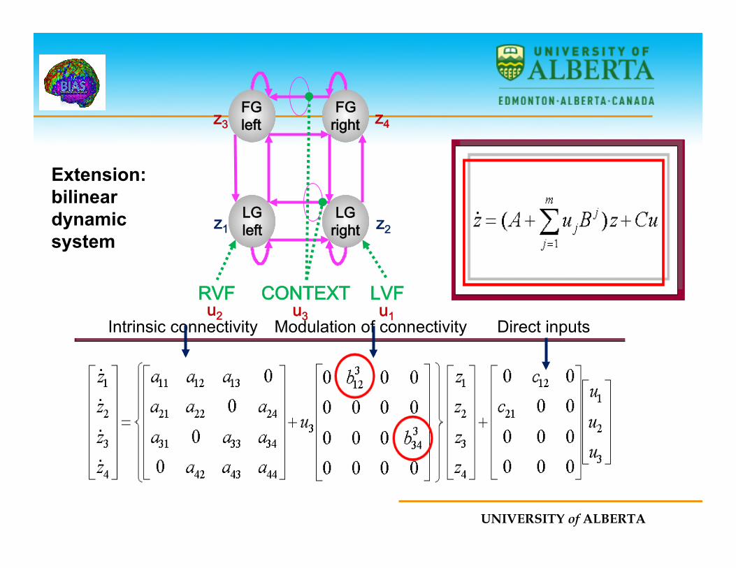
Extension: bilinear dynamic system
LG left
LG right
RVF LVF
FG right
FG left
z1 z2
z4 z3
u2 u1
CONTEXT u3
Intrinsic connectivity Direct inputs Modulation of connectivity
UNIVERSITY of ALBERTA
UNIVERSITY of ALBERTA
Hemodynamics
Ø The neuronal activities in each region cause changes in blood volume and deoxyhmoglobin that, in turn, cause changes in the observed BOLD response.
Ø The hemodynamics are described using an extended Balloon model, which involves a set of hemodynamic state variables, state equations and hemodynamic parameters θh.
UNIVERSITY of ALBERTA
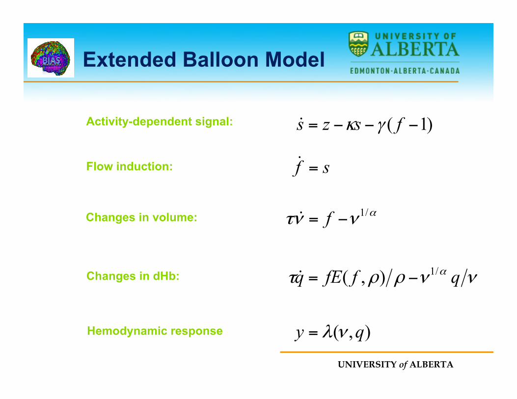
)1( −−−= fszs γκ!
sf =!
ανντ /1−= f!
ννρρτ α qffEq /1),( −=!
),( qy νλ=
Extended Balloon Model
Activity-dependent signal:
Flow induction:
Changes in volume:
Changes in dHb:
Hemodynamic response
UNIVERSITY of ALBERTA
sftionflow induc
=!
s
v
f
vq q/vvf,Efqτ /α
dHbchanges in1)( −= ρρ!/αvfvτ
volumechanges in1−=!
f
q
)1( −−−= fγszsry signalvasodilato
κ!
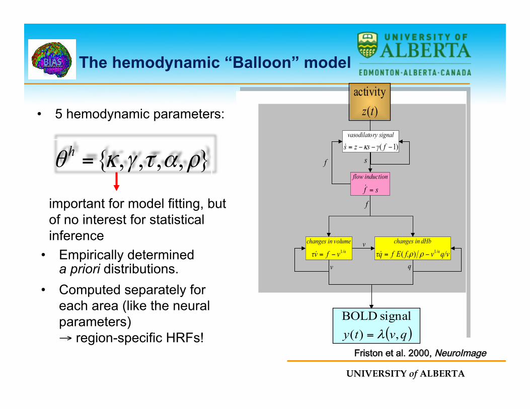
},,,,{ ρατγκθ =h
important for model fitting, but of no interest for statistical inference
( ) ,)( signal BOLDqvty λ=
The hemodynamic “Balloon” model
)(activity
tz• 5 hemodynamic parameters:
• Empirically determined a priori distributions.
• Computed separately for each area (like the neural parameters) → region-specific HRFs!
Friston et al. 2000, NeuroImage
UNIVERSITY of ALBERTA
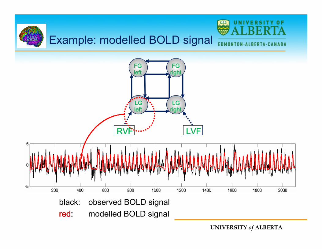
LG left
LG right
RVF LVF
FG right
FG left
Example: modelled BOLD signal
black: observed BOLD signal red: modelled BOLD signal
UNIVERSITY of ALBERTA
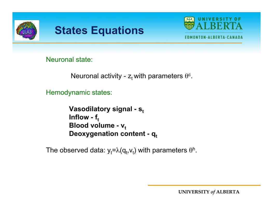
States Equations
Neuronal state:
Neuronal activity - zt with parameters θc. Hemodynamic states:
Vasodilatory signal - st Inflow - ft Blood volume - vt Deoxygenation content - qt
The observed data: yt=λ(qt,vt) with parameters θh.
UNIVERSITY of ALBERTA
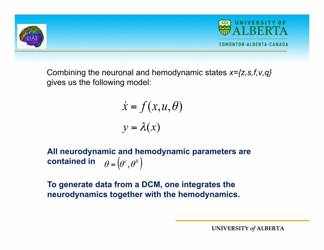
Combining the neuronal and hemodynamic states x={z,s,f,v,q} gives us the following model:
),,( θuxfx =!)(xy λ=
All neurodynamic and hemodynamic parameters are contained in To generate data from a DCM, one integrates the neurodynamics together with the hemodynamics.
( )hc θθθ ,=
UNIVERSITY of ALBERTA
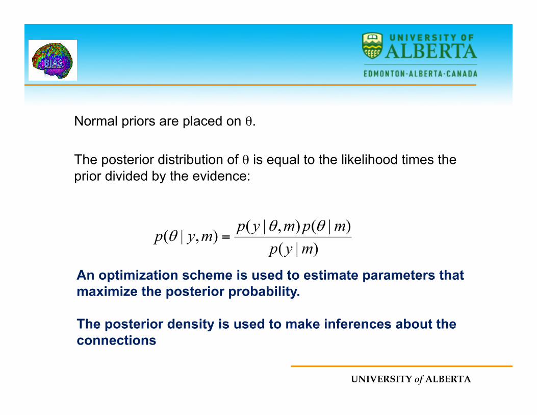
Normal priors are placed on θ. The posterior distribution of θ is equal to the likelihood times the prior divided by the evidence:
)|()|(),|(),|(
mypmpmypmyp θθ
θ =
An optimization scheme is used to estimate parameters that maximize the posterior probability. The posterior density is used to make inferences about the connections
UNIVERSITY of ALBERTA
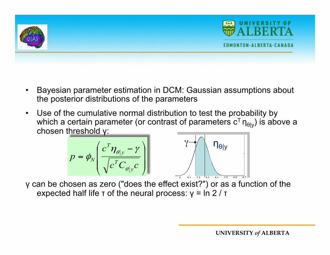
• Bayesian parameter estimation in DCM: Gaussian assumptions about the posterior distributions of the parameters
• Use of the cumulative normal distribution to test the probability by which a certain parameter (or contrast of parameters cT ηθ|y) is above a chosen threshold γ:
γ can be chosen as zero ("does the effect exist?") or as a function of the expected half life τ of the neural process: γ = ln 2 / τ
⎟⎟⎟
⎠
⎞
⎜⎜⎜
⎝
⎛ −=
cCc
cp
yT
yT
N
θ
θ γηφ
γ ηθ|y
UNIVERSITY of ALBERTA
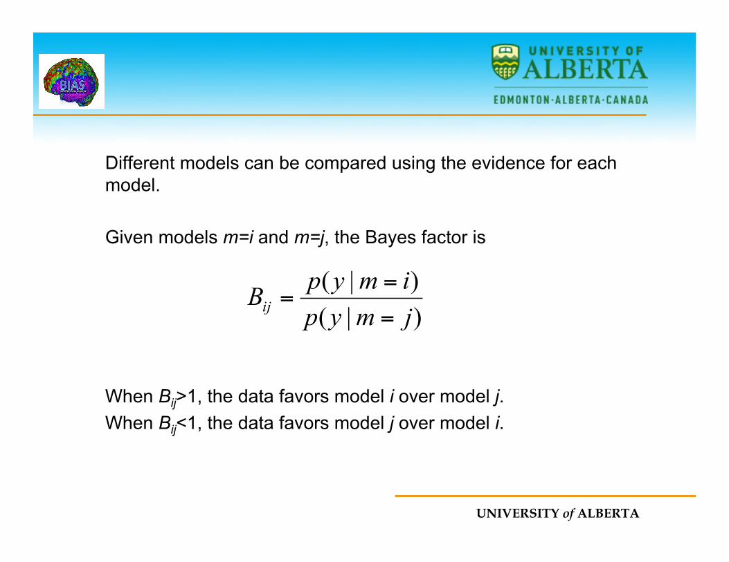
Different models can be compared using the evidence for each model. Given models m=i and m=j, the Bayes factor is When Bij>1, the data favors model i over model j. When Bij<1, the data favors model j over model i.
)|()|(jmypimypBij =
==
UNIVERSITY of ALBERTA
Comments
Ø DCM models interactions at the neuronal rather than the hemodynamic level.
Ø It is therefore more biologically accurate than the other models described today.
Ø However, it is quite computationally demanding. It is limited to 8 regions in SPM.
UNIVERSITY of ALBERTA
Granger Causality
Ø Granger causality is a technique that was originally developed in economics that has recently been applied to connectivity studies.
Ø It does not rely on the a priori specification of a structural model, but rather is an approach for quantifying the usefulness of past values from various brain regions in predicting current values in other regions.
Ø Granger causality provides information about the temporal precedence of relationships among two regions, but it is in some sense a misnomer because it does not actually provide information about causality.
UNIVERSITY of ALBERTA
Set Up
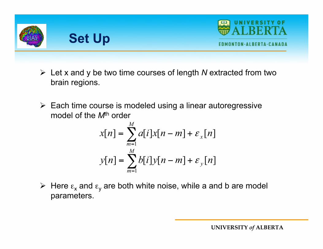
Ø Let x and y be two time courses of length N extracted from two brain regions.
Ø Each time course is modeled using a linear autoregressive model of the Mth order
Ø Here εx and εy are both white noise, while a and b are model parameters.
][][][][1
nmnxianx x
M
mε+−=∑
=
][][][][1
nmnyibny y
M
mε+−=∑
=
UNIVERSITY of ALBERTA
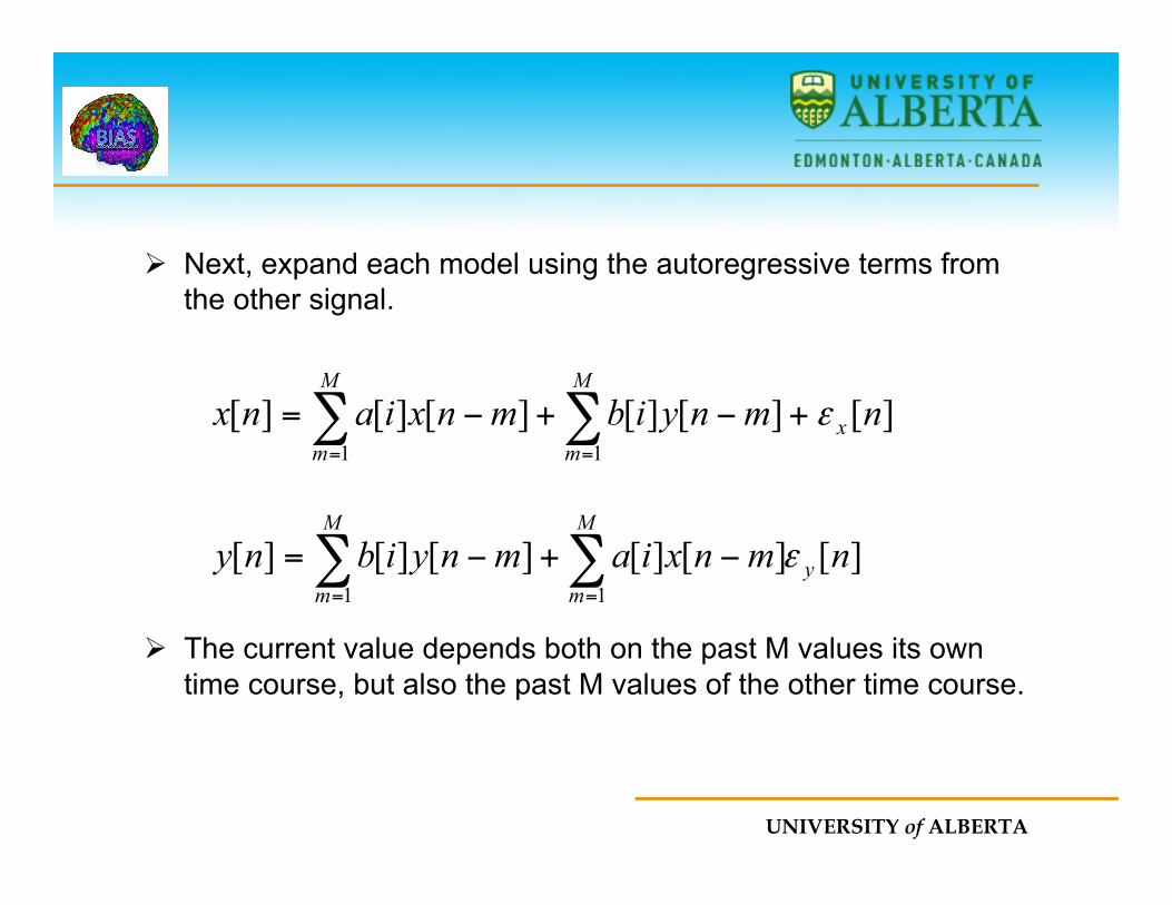
Ø Next, expand each model using the autoregressive terms from the other signal.
Ø The current value depends both on the past M values its own time course, but also the past M values of the other time course.
][][][][][][11
nmnyibmnxianx x
M
m
M
mε+−+−= ∑∑
==
][][][][][][11
nmnxiamnyibny y
M
m
M
mε∑∑
==
−+−=

UNIVERSITY of ALBERTA
Ø Using these models one can test whether the history of x has any predictive value on the current value of y (and vice versa).
Ø If the model fit is significantly improved by the inclusion of the cross-autoregressive terms, it provides evidence that the history of one of the time courses can be used to predict the current value of the other and a “Granger-causal” relationship is inferred.
UNIVERSITY of ALBERTA
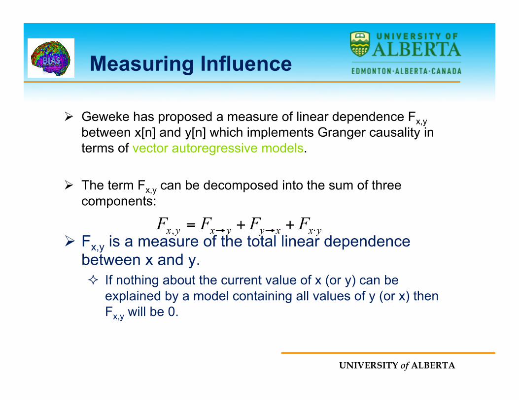
Measuring Influence
Ø Geweke has proposed a measure of linear dependence Fx,y between x[n] and y[n] which implements Granger causality in terms of vector autoregressive models.
Ø The term Fx,y can be decomposed into the sum of three components:
Ø Fx,y is a measure of the total linear dependence between x and y. ² If nothing about the current value of x (or y) can be
explained by a model containing all values of y (or x) then Fx,y will be 0.
yxxyyxyx FFFF ⋅→→ ++=,
UNIVERSITY of ALBERTA
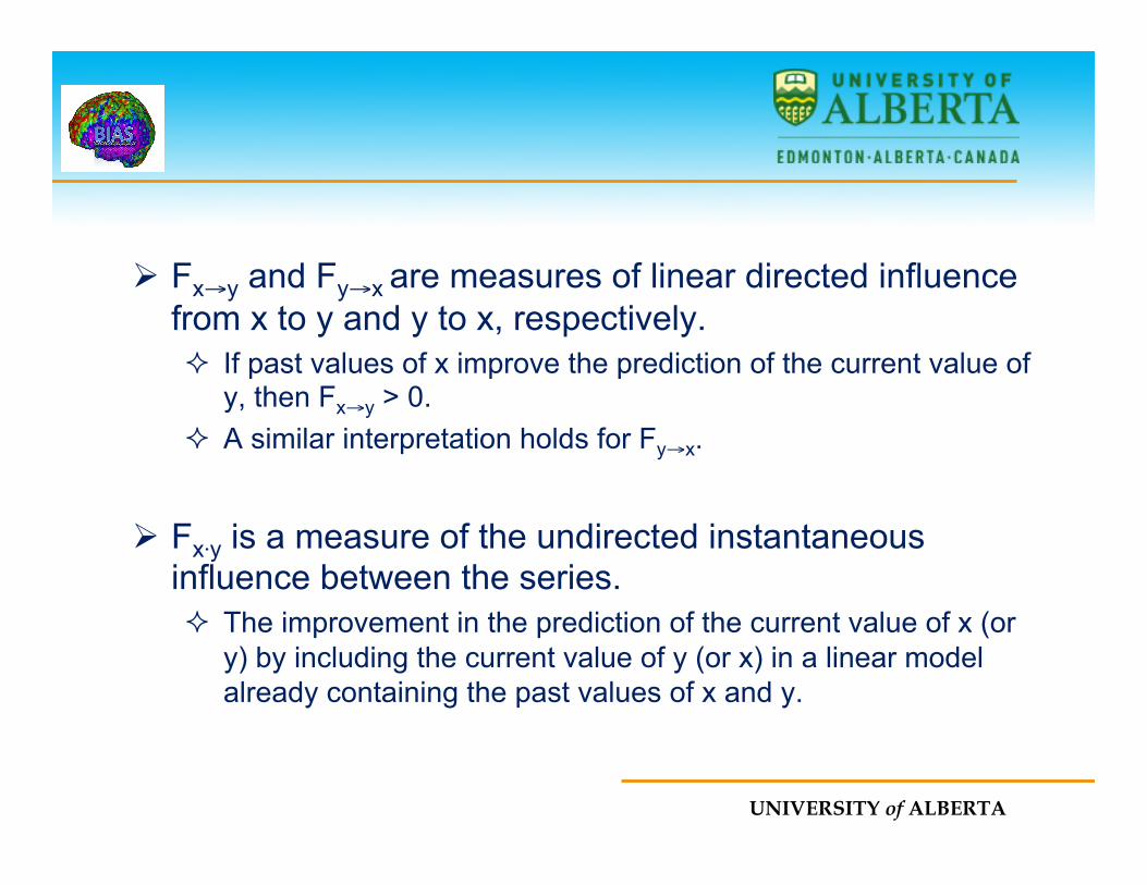
Ø Fx→y and Fy→x are measures of linear directed influence from x to y and y to x, respectively. ² If past values of x improve the prediction of the current value of
y, then Fx→y > 0. ² A similar interpretation holds for Fy→x.
Ø Fx⋅y is a measure of the undirected instantaneous influence between the series. ² The improvement in the prediction of the current value of x (or
y) by including the current value of y (or x) in a linear model already containing the past values of x and y.
UNIVERSITY of ALBERTA
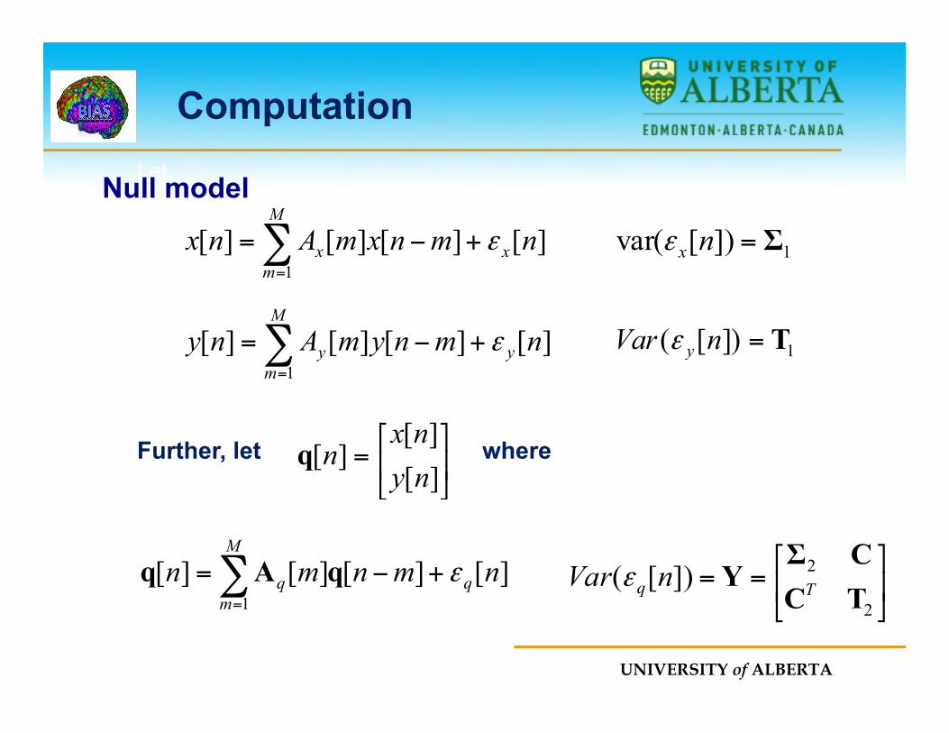
][][][][1
nmnxmAnx x
M
mx ε+−=∑
=1])[var( Σ=nxε
Let,
][][][][1
nmnymAny y
M
my ε+−=∑
=1])[( T=nVar yε
][][][][1
nmnmn q
M
mq ε+−=∑
=
qAq ⎥⎦
⎤⎢⎣
⎡==
2
2])[(TCCΣ
Y Tq nVar ε
Further, let where ⎥⎦
⎤⎢⎣
⎡=
][][
][nynx
nq
Computation
Null model
UNIVERSITY of ALBERTA
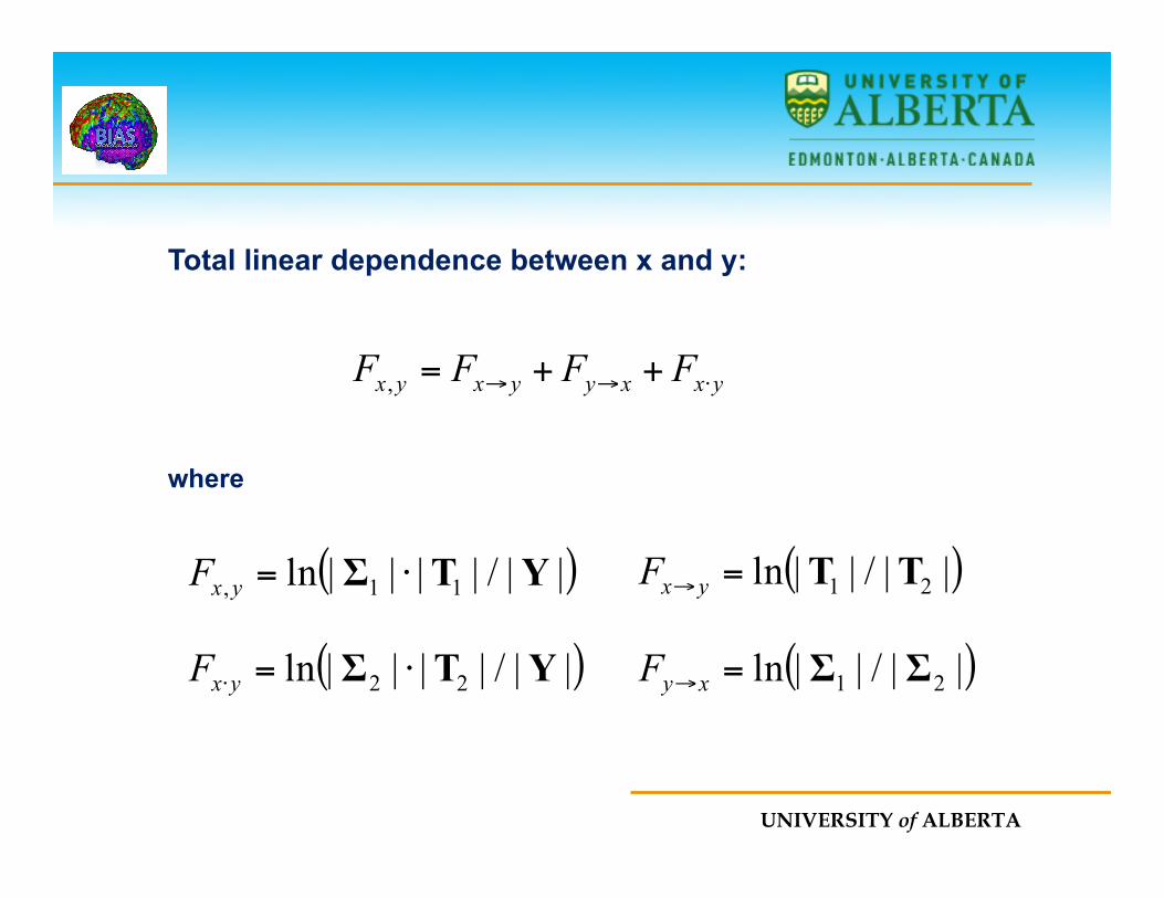
( )||/||||ln 11, YTΣ ⋅=yxF ( )||/||ln 21 TT=→yxF
( )||/||ln 21 ΣΣ=→xyF( )||/||||ln 22 YTΣ ⋅=⋅yxF
yxxyyxyx FFFF ⋅→→ ++=,
Total linear dependence between x and y:
where
UNIVERSITY of ALBERTA
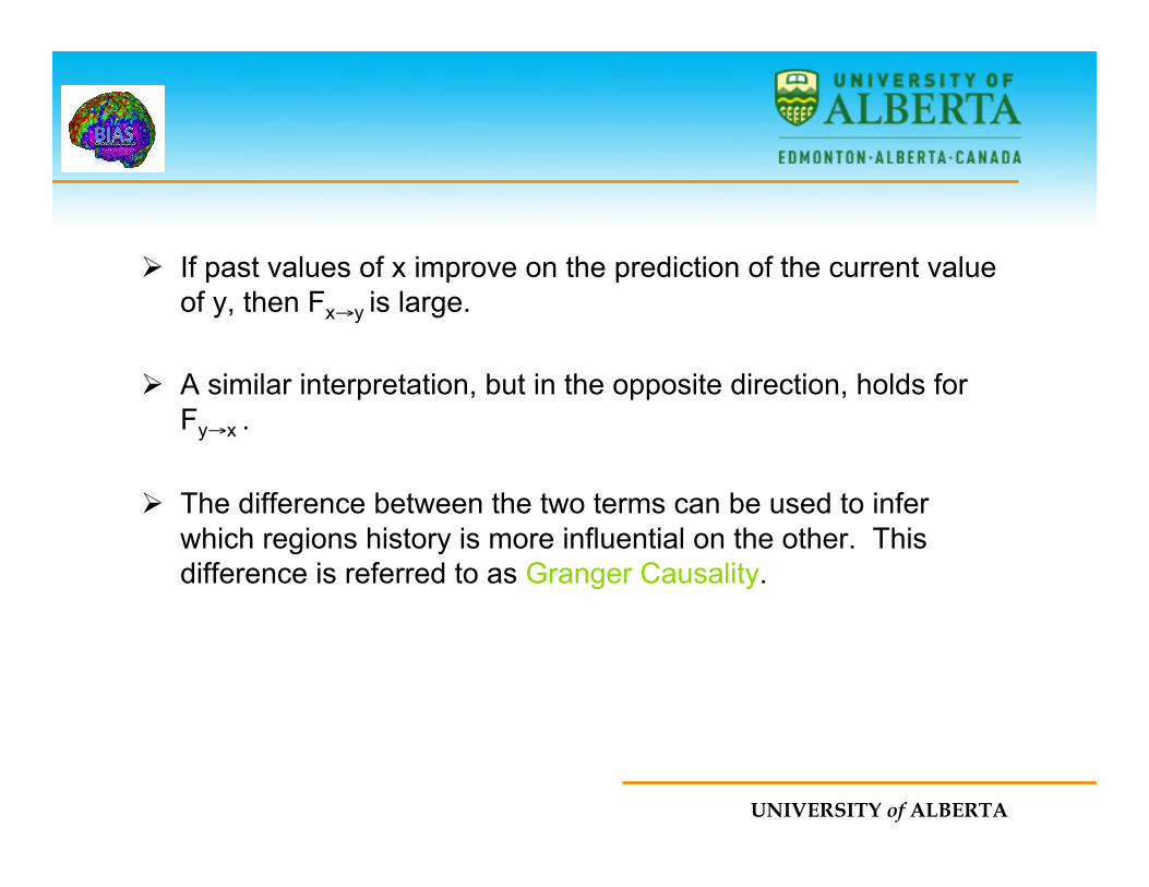
Ø If past values of x improve on the prediction of the current value of y, then Fx→y is large.
Ø A similar interpretation, but in the opposite direction, holds for Fy→x .
Ø The difference between the two terms can be used to infer which regions history is more influential on the other. This difference is referred to as Granger Causality.
UNIVERSITY of ALBERTA
Granger Causality Map
Ø A Granger Causality Map (GCM) is computed with respect to a single selected reference region (e.g., seed region).
Ø It maps both sources of influence to the reference region and targets of influence from the reference region over the brain.
UNIVERSITY of ALBERTA
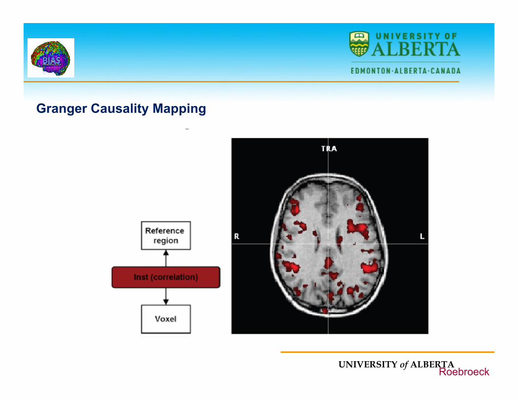
Granger Causality Mapping
Roebroeck
UNIVERSITY of ALBERTA
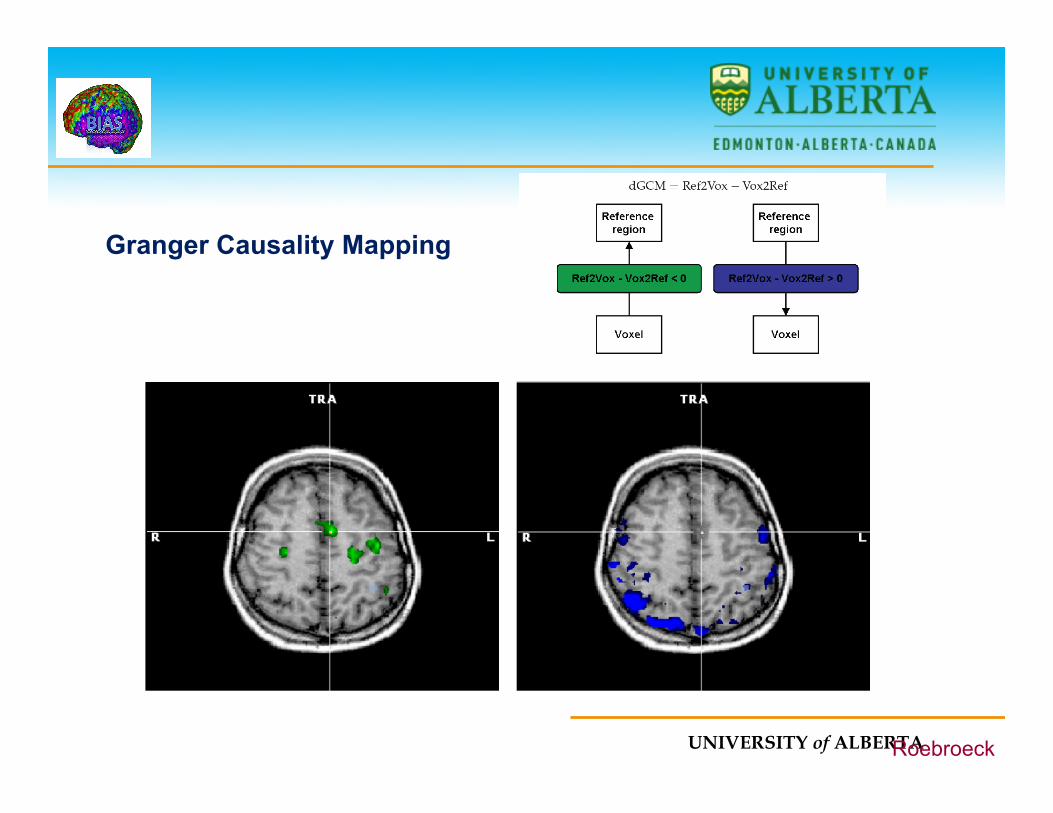
Granger Causality Mapping
Roebroeck