Embed Size (px)
Citation preview
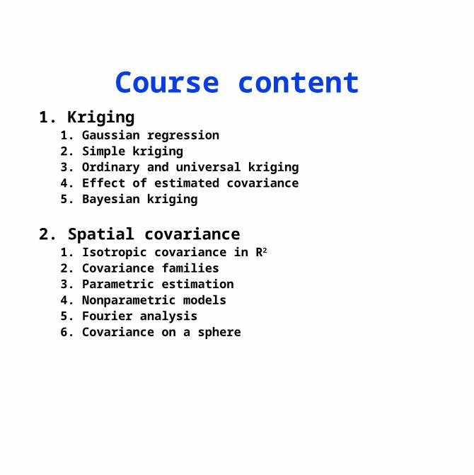
Course content1. Kriging 1. Gaussian regression 2. Simple kriging 3. Ordinary and universal kriging 4. Effect of estimated covariance 5. Bayesian kriging
2. Spatial covariance 1. Isotropic covariance in R2
2. Covariance families 3. Parametric estimation 4. Nonparametric models 5. Fourier analysis 6. Covariance on a sphere
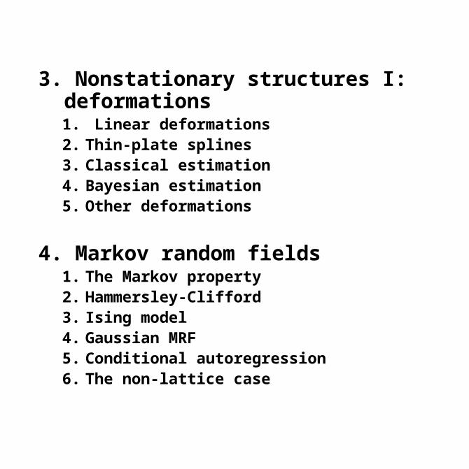
3. Nonstationary structures I: deformations1. Linear deformations2. Thin-plate splines3. Classical estimation4. Bayesian estimation5. Other deformations
4. Markov random fields1. The Markov property2. Hammersley-Clifford3. Ising model4. Gaussian MRF5. Conditional autoregression6. The non-lattice case

5. Nonstationary structures II: linear combinations etc.
1.Moving window kriging2.Integrated white noise3.Spectral methods4.Testing for nonstationarity
5.Kernel methods
6. Space-time models1.Mean surface2.Separability3.A simple non-separable model4.Stationary space-time processes5.Space-time covariance models6.Testing for separability

7. Statistics, data and deterministic models
1. The kriging approach2. Bayesian hierarchical models3. Bayesian melding4. Data assimilation5. Model approximation
8. Setting air quality standards1. Health effect studies2. Standards as hypothesis tests3. Potential network bias4. What are people exposed to5. A framework for setting standards
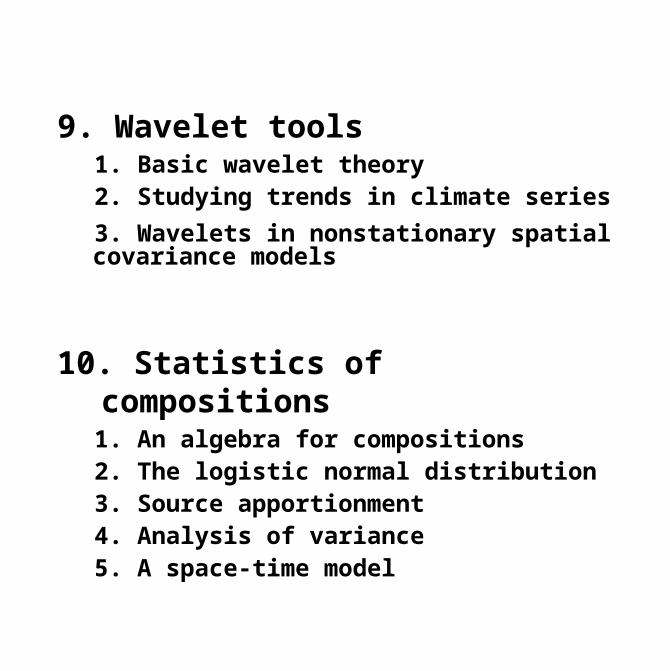
9. Wavelet tools1. Basic wavelet theory2. Studying trends in climate series
3. Wavelets in nonstationary spatial covariance models
10. Statistics of compositions1. An algebra for compositions2. The logistic normal distribution3. Source apportionment4. Analysis of variance5. A space-time model

Programs
RgeoR
Fields
S-PlusS+ SpatialStats

Kriging
NRCSE
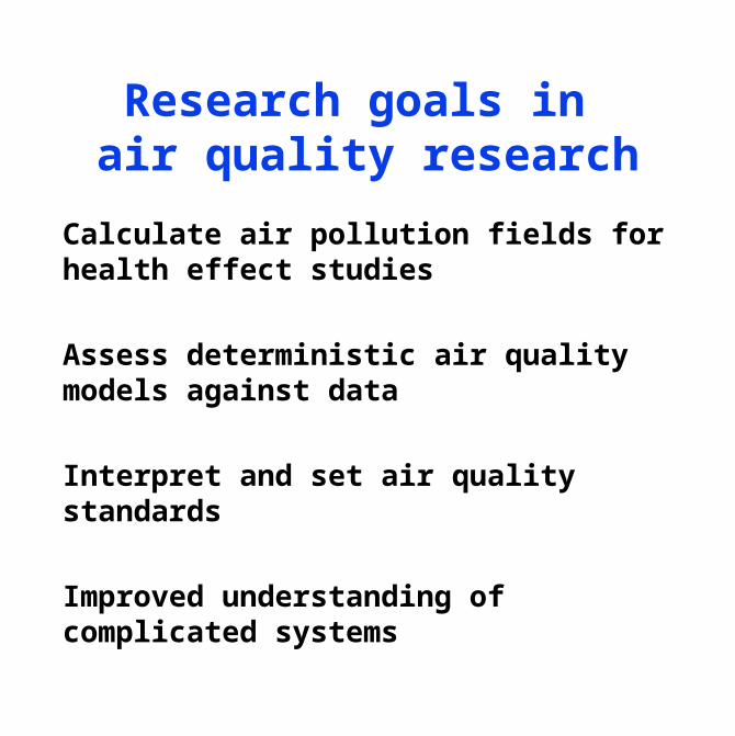
Research goals in air quality research
Calculate air pollution fields for health effect studies
Assess deterministic air quality models against data
Interpret and set air quality standards
Improved understanding of complicated systems
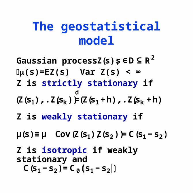
The geostatistical model
Gaussian process(s)=EZ(s) Var Z(s) < ∞Z is strictly stationary if
Z is weakly stationary if
Z is isotropic if weakly stationary and
Z(s),s ∈D⊆R2
(Z(s1),...,Z(sk))=d(Z(s1+h),...,Z(sk +h))
μ(s)≡μ Cov(Z(s1),Z(s2))=C(s1−s2)
C(s1−s2)=C0(s1−s2 )

The problem
Given observations at n locationsZ(s1),...,Z(sn)
estimate
Z(s0) (the process at an unobserved
location)
(an average of the process)
In the environmental context often time series of observations at the locations.
Z(s)dν(s)A∫or

Some history
Regression (Galton, Bartlett)
Mining engineers (Krige 1951, Matheron, 60s)
Spatial models (Whittle, 1954)
Forestry (Matérn, 1960)
Objective analysis (Grandin, 1961)
More recent work Cressie (1993), Stein (1999)

A Gaussian formula
If
then
€
X
Y
⎛
⎝ ⎜
⎞
⎠ ⎟~ N
μX
μY
⎛
⎝ ⎜
⎞
⎠ ⎟,
ΣXX ΣXY
ΣYX ΣYY
⎛
⎝ ⎜
⎞
⎠ ⎟
⎛
⎝ ⎜
⎞
⎠ ⎟
€
(Y |X) ~ N(μY + ΣYXΣXX−1 (X −μX ),
ΣYY − ΣYXΣXX−1 ΣXY )
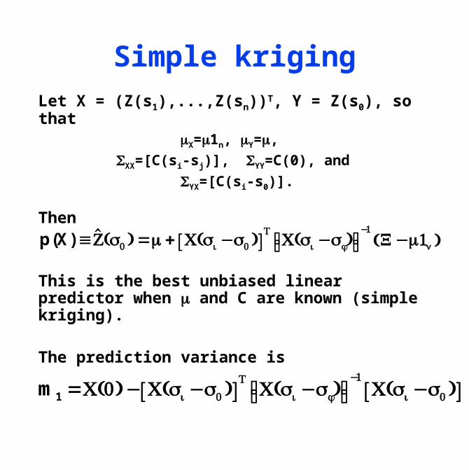
Simple kriging
Let X = (Z(s1),...,Z(sn))T, Y = Z(s0), so thatX=1n, Y=,
XX=[C(si-sj)], YY=C(0), and
YX=[C(si-s0)].
Then
This is the best unbiased linear predictor when and C are known (simple kriging).
The prediction variance is
p(X) ≡Z(s0 ) = + C(s i −s0 )[ ]T
C(s i −s j )⎡⎣ ⎤⎦−1
X−1n( )
m1 =C(0) − C(s i −s0 )[ ]T
C(s i −s j )⎡⎣ ⎤⎦−1
C(s i −s0 )[ ]
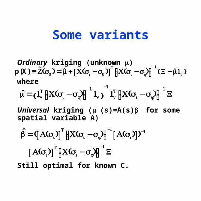
Some variants
Ordinary kriging (unknown )
where
Universal kriging ( (s)=A(s) for some spatial variable A)
Still optimal for known C.
p(X) ≡Z(s0 ) = + C(s i −s0 )[ ]T
C(s i −s j )⎡⎣ ⎤⎦−1
X−1n( )
= 1nT C(s i −s j )⎡⎣ ⎤⎦
−11n( )
−1
1nT C(s i −s j )⎡⎣ ⎤⎦
−1X
=( A(s i )[ ]T
C(s i −s j )⎡⎣ ⎤⎦−1
A(s i )[ ])−1
A(s i )[ ]T
C(s i −s j )⎡⎣ ⎤⎦−1
X
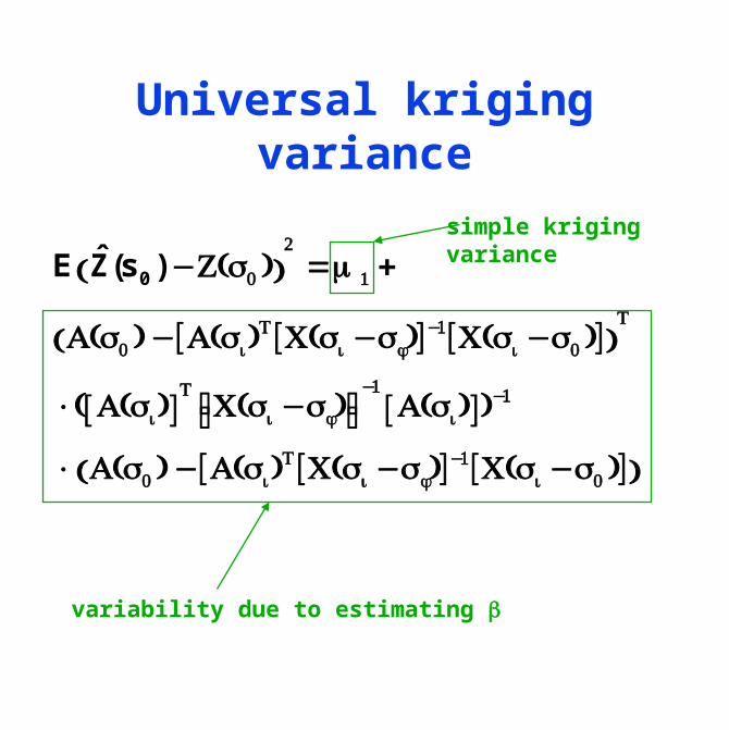
Universal kriging variance
E Z(s0 ) −Z(s0 )( )2=m1 +
A(s0 ) −[A(s i )T [C(s i −s j )]
−1[C(s i −s0 )]( )T
×( A(s i )[ ]T
C(s i −s j )⎡⎣ ⎤⎦−1
A(s i )[ ])−1
× A(s0 ) −[A(s i )T [C(s i −s j )]
−1[C(s i −s0 )]( )
simple kriging variance
variability due to estimating

The (semi)variogram
Intrinsic stationarity
Weaker assumption (C(0) needs not exist)
Kriging predictions can be expressed in terms of the variogram instead of the covariance.
γ( h ) =1
2Var(Z(s + h) − Z(s)) = C(0) − C( h )
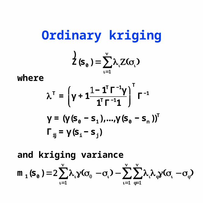
Ordinary kriging
where
and kriging variance
)Z(s0 ) = λ iZ(s i )
i=1
n
∑
λT = γ + 11− 1T Γ−1γ
1T Γ−11
⎛
⎝⎜⎞
⎠⎟
T
Γ−1
γ = (γ(s0 − s1),...,γ(s0 − sn ))T
Γ ij = γ(si − s j )
m1(s0 ) =2 λ iγ(s0 −s i )i=1
n
∑ − λ iλ jγ(s i −s j )j=1
n
∑i=1
n
∑

An example
Ozone data from NE USA (median of daily one hour maxima June–August 1974, ppb)
QuickTime™ and aTIFF (Uncompressed) decompressor
are needed to see this picture.
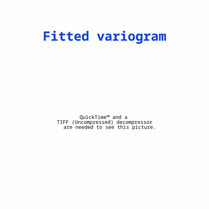
Fitted variogram
€
γ(t) = σe2 + σs
2 1− e− t
θ ⎛ ⎝ ⎜
⎞ ⎠ ⎟
QuickTime™ and aTIFF (Uncompressed) decompressor
are needed to see this picture.

QuickTime™ and aTIFF (Uncompressed) decompressor
are needed to see this picture.
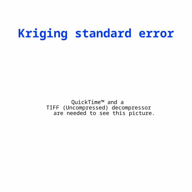
Kriging surface
QuickTime™ and aTIFF (Uncompressed) decompressor
are needed to see this picture.
Kriging standard error
QuickTime™ and aTIFF (Uncompressed) decompressor
are needed to see this picture.
A better combination
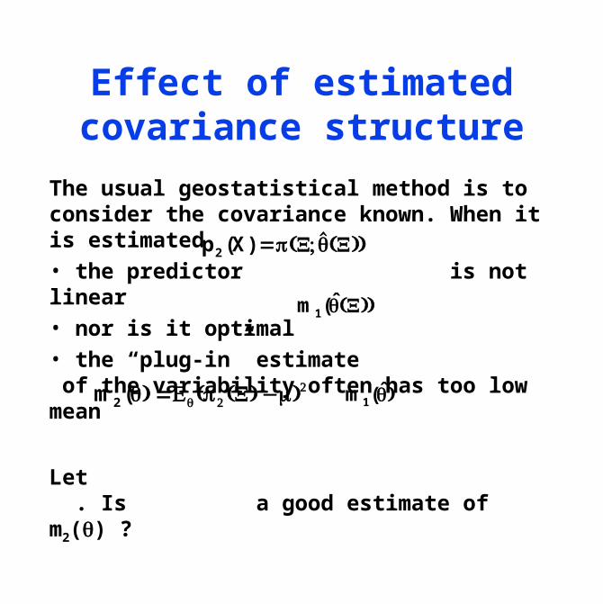
Effect of estimated covariance structure
The usual geostatistical method is to consider the covariance known. When it is estimated
• the predictor is not linear
• nor is it optimal
• the “plug-in” estimate of the variability often has too low mean
Let . Is a good estimate of m2() ?
p2 (X) =p(X; (X))
m1((X))
m2 () =E (p2 (X) −)2 m1()
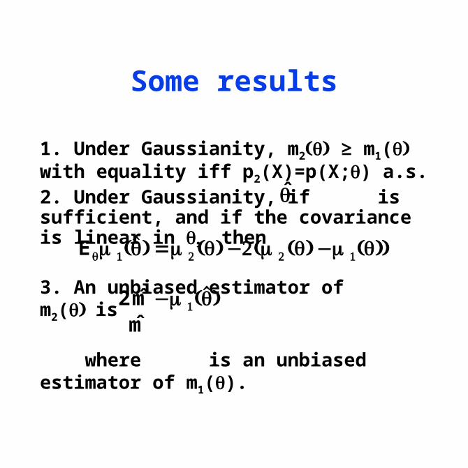
Some results
1. Under Gaussianity, m2 ≥ m1( with equality iff p2(X)=p(X;) a.s.2. Under Gaussianity, if is sufficient, and if the covariance is linear in then
3. An unbiased estimator of m2( is
where is an unbiased estimator of m1().
Em1() =m2 () −2(m2 () −m1())
2m−m1()m
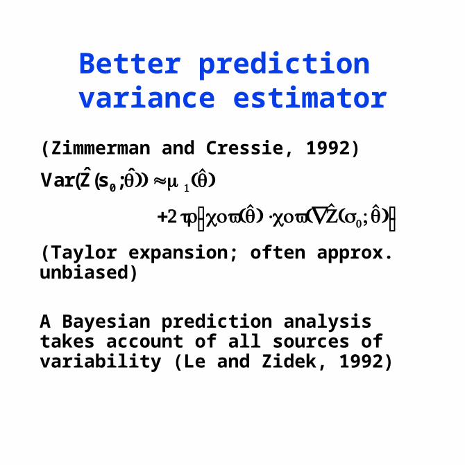
Better prediction variance estimator
(Zimmerman and Cressie, 1992)
(Taylor expansion; often approx. unbiased)
A Bayesian prediction analysis takes account of all sources of variability (Le and Zidek, 1992)
Var(Z(s0; )) ≈m1()
+2 tr cov() ⋅cov(∇Z(s0; )⎡⎣
⎤⎦
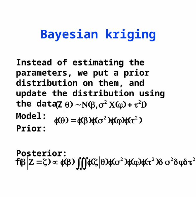
Bayesian kriging
Instead of estimating the parameters, we put a prior distribution on them, and update the distribution using the data.
Model:
Prior:
Posterior:
(Z ) ~N(,σ2 C(φ) + τ2I)
f() =f()f(σ2 )f(φ)f(τ2 )
f( Z=z) ∝ f() f(z )f(σ2 )f(φ)f(τ2 )d∫∫∫ σ2dφdτ2

geoR
Default covariance model exponential
Prior is assigned to and . The latter assumed zero unless specified.
The distributions can be discretized.
Default prior on is flat (if not specified, assumed constant).
(Lots of different assignments are possible)
τ σ

Prior/posterior of
QuickTime™ and aTIFF (Uncompressed) decompressor
are needed to see this picture.

QuickTime™ and aTIFF (Uncompressed) decompressor
are needed to see this picture.
Variogram estimates
meanmedianmode

QuickTime™ and aTIFF (Uncompressed) decompressor
are needed to see this picture.
Predictive mean
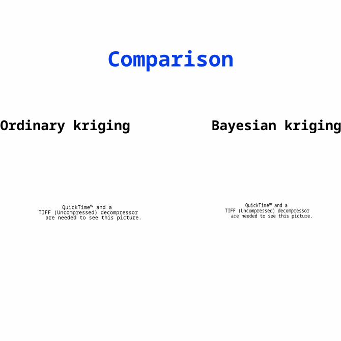
Comparison
Ordinary kriging Bayesian kriging
QuickTime™ and aTIFF (Uncompressed) decompressor
are needed to see this picture.
QuickTime™ and aTIFF (Uncompressed) decompressor
are needed to see this picture.

QuickTime™ and aTIFF (Uncompressed) decompressor
are needed to see this picture.
Kriging variances
Bayes Classical
range (52,307) range (170,278)
Practical exercises
Lectures, references, and labs will be made available athttp://www.stat.washington.edu/peter/brisbane