Statistics 349.3(02)

Analysis of Time Series

Course Information

1. Instructor:• W. H. Laverty• 235 McLean Hall• Tel: 966-6096 Email: laverty@math.usask.ca

2. Class Times• MWF 12:30-1:20pm Geology 269

3. Mark break-up• Final Exam – 60%• Term Tests and Assignments – 40%

Course Outline

1. Introduction and Review of Probability Theory– Probability distributions, Expectation,

Variance, correlation– Sampling distributions– Estimation Theory– Hypothesis Testing

Course Outline -continued

2. Fundamental concepts in Time Series Analysis– Stationarity– Autocovariance function, autocorrelation and partial

autocorrelation function3. Models for Stationary Time series

– Autoregressive (AR), Moving average (MA), mixed Autoregressive-Moving average (ARMA) models

4. Models for Non-stationary Time series– ARIMA (Integrated Autoregressive-Moving average

models)

Course Outline -continued

5. Forecasting ARIMA Processes6. Model Identification and Estimation7. Models for seasonal Time series8. Spectral Analysis of Time series

Course Outline -continued

9. State-Space modeling of time series, Hidden Markov Model (HMM)

– Kalman filtering10. Multivariate (Multi-channel) time series

analysis11. Linear filtering

Comments

• The Text Book– Introduction to Statistical Time Series, 2nd

Edition, Wayne A. Fuller• I will present the material in power point slides

that will be available on my web site.• Hopefully this makes purchasing the text book

optional. It is useful for students to purchase text books and build up a library.

Some examples

of Time series data

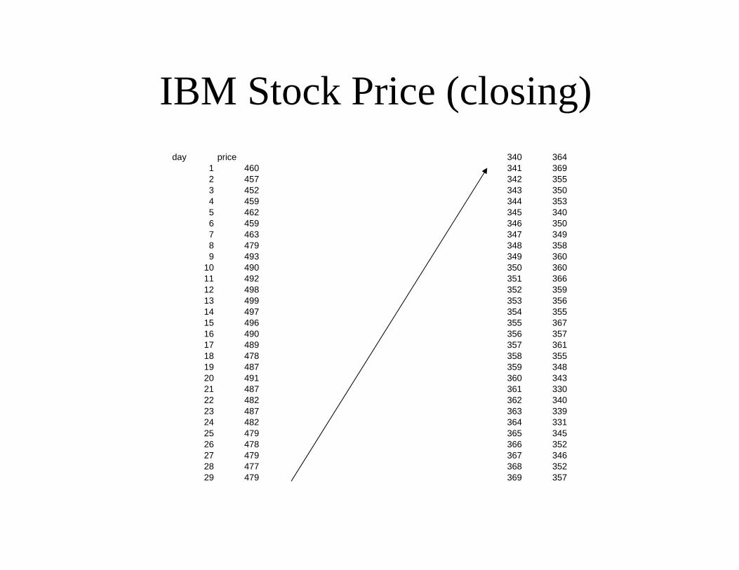
IBM Stock Price (closing)day price

1 4602 4573 4524 4595 4626 4597 4638 4799 493

10 49011 49212 49813 49914 49715 49616 49017 48918 47819 48720 49121 48722 48223 48724 48225 47926 47827 47928 47729 479

340 364341 369342 355343 350344 353345 340346 350347 349348 358349 360350 360351 366352 359353 356354 355355 367356 357357 361358 355359 348360 343361 330362 340363 339364 331365 345366 352367 346368 352369 357

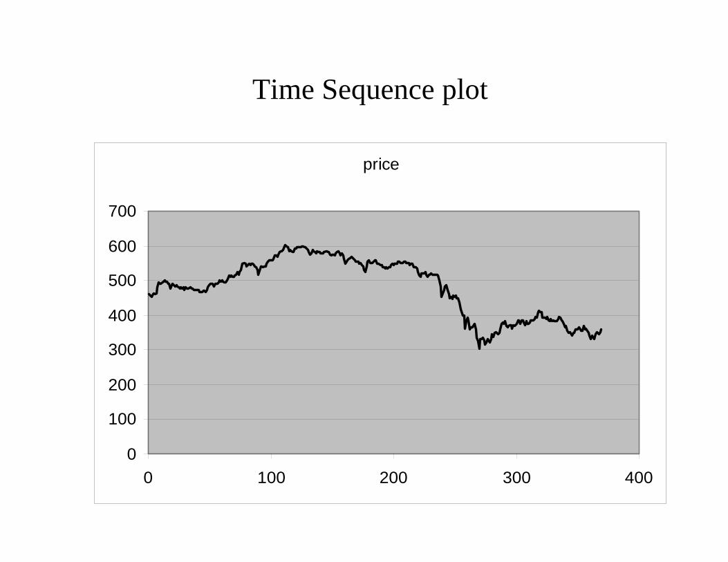
Time Sequence plot

price

0

100

200

300

400

500

600

700

0 100 200 300 400

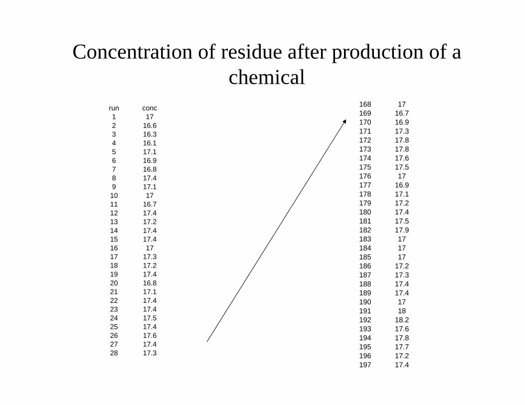
Concentration of residue after production of a chemical

run conc1 172 16.63 16.34 16.15 17.16 16.97 16.88 17.49 17.110 1711 16.712 17.413 17.214 17.415 17.416 1717 17.318 17.219 17.420 16.821 17.122 17.423 17.424 17.525 17.426 17.627 17.428 17.3

168 17169 16.7170 16.9171 17.3172 17.8173 17.8174 17.6175 17.5176 17177 16.9178 17.1179 17.2180 17.4181 17.5182 17.9183 17184 17185 17186 17.2187 17.3188 17.4189 17.4190 17191 18192 18.2193 17.6194 17.8195 17.7196 17.2197 17.4

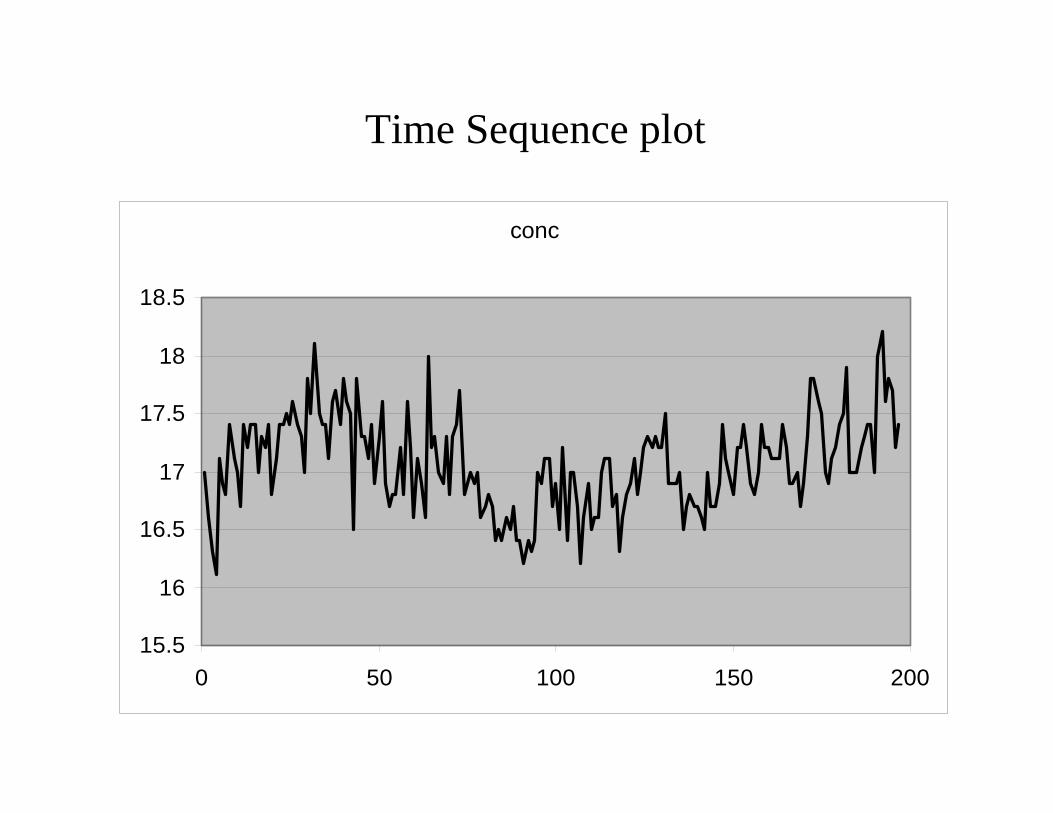
Time Sequence plot

conc

15.5

16

16.5

17

17.5

18

18.5

0 50 100 150 200

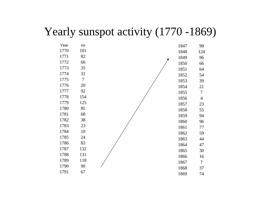
Yearly sunspot activity (1770 -1869)Year no1770 1011771 821772 661773 351774 311775 71776 201777 921778 1541779 1251780 851781 681782 381783 231784 101785 241786 831787 1321788 1311789 1181790 901791 67

1847 981848 1241849 961850 661851 641852 541853 391854 211855 71856 41857 231858 551859 941860 961861 771862 591863 441864 471865 301866 161867 71868 371869 74

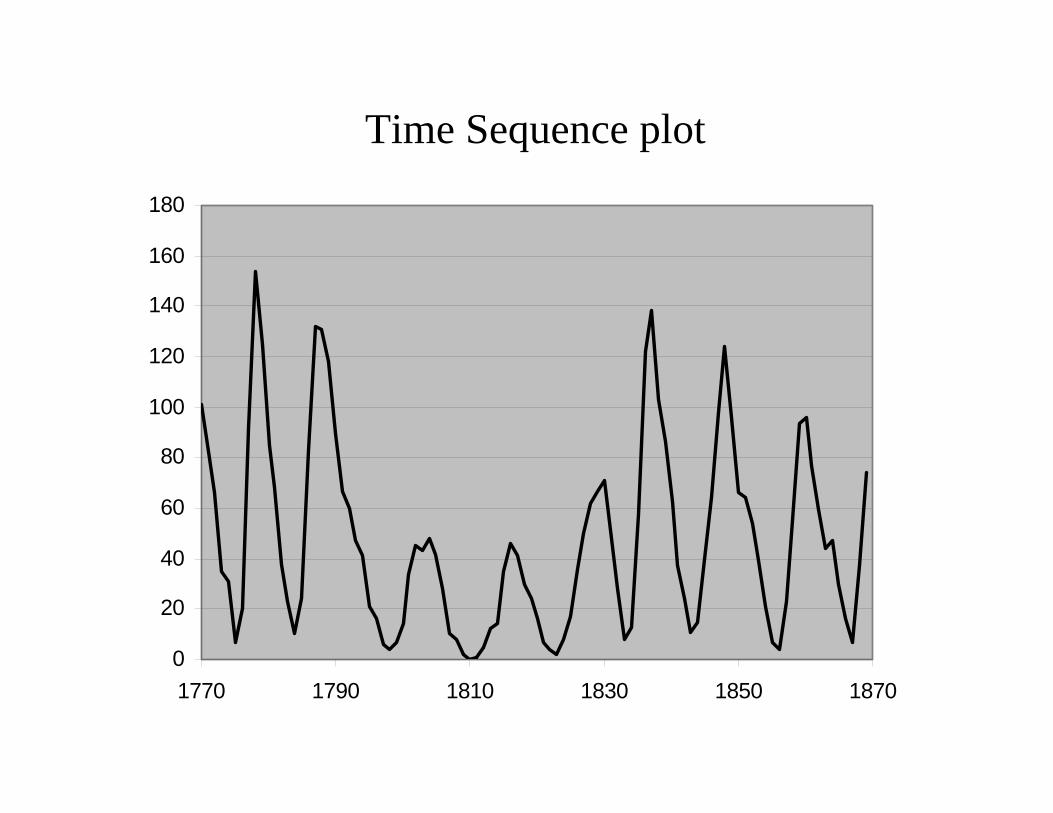
Time Sequence plot

0

20

40

60

80

100

120

140

160

180

1770 1790 1810 1830 1850 1870

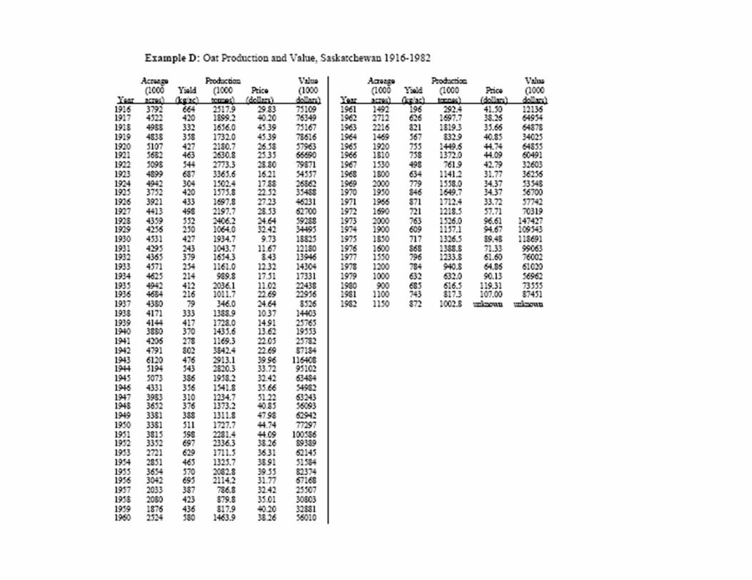
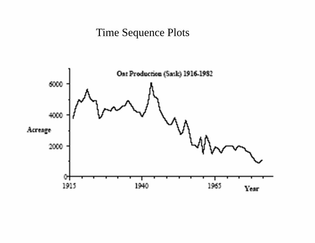
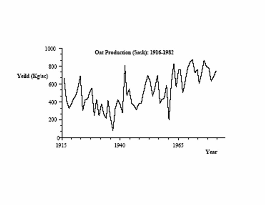
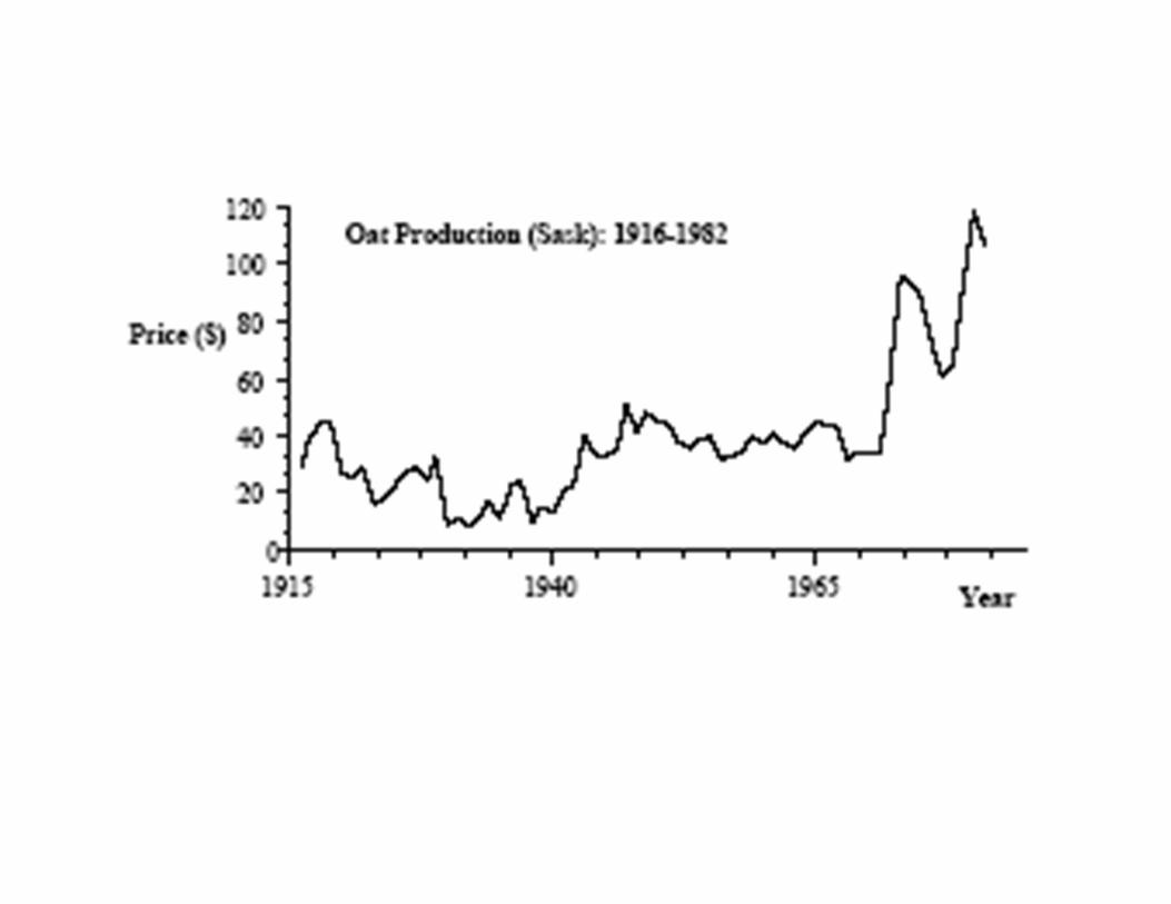
Time Sequence Plots

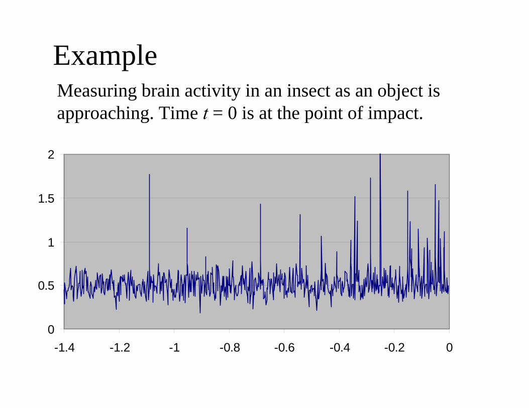
ExampleMeasuring brain activity in an insect as an object is approaching. Time t = 0 is at the point of impact.

0

0.5

1

1.5

2

-1.4 -1.2 -1 -0.8 -0.6 -0.4 -0.2 0

Simulation

To aid in the understanding of time series it is useful to simulate data

Generating observations from a distribution

Generating a random number from a distribution

Let1. f(x) denote the density function2. F(x) denote the cumulative distribution

function = P[X ≤ x]3. F-1(x) denote the inverse cumulative

distribution function

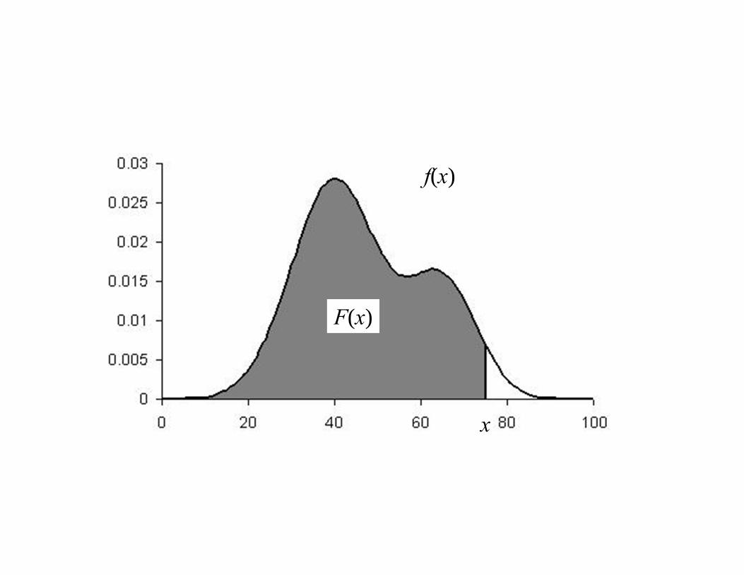
F(x) denote the cumulative distribution function

F(x)

f(x)

x

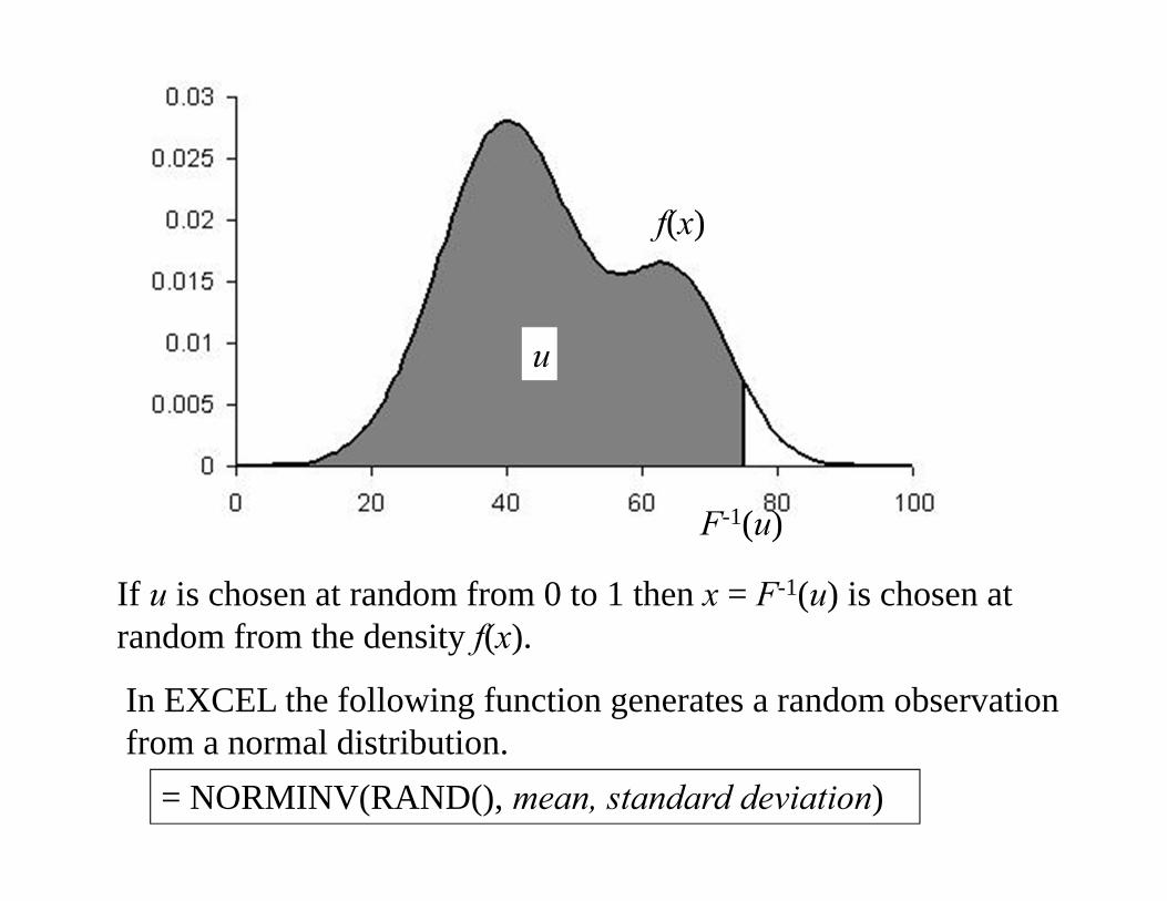
F(x) denote the cumulative distribution function

u

f(x)

F-1(u)

If u is chosen at random from 0 to 1 then x = F-1(u) is chosen at random from the density f(x).

In EXCEL the following function generates a random observation from a normal distribution.

= NORMINV(RAND(), mean, standard deviation)

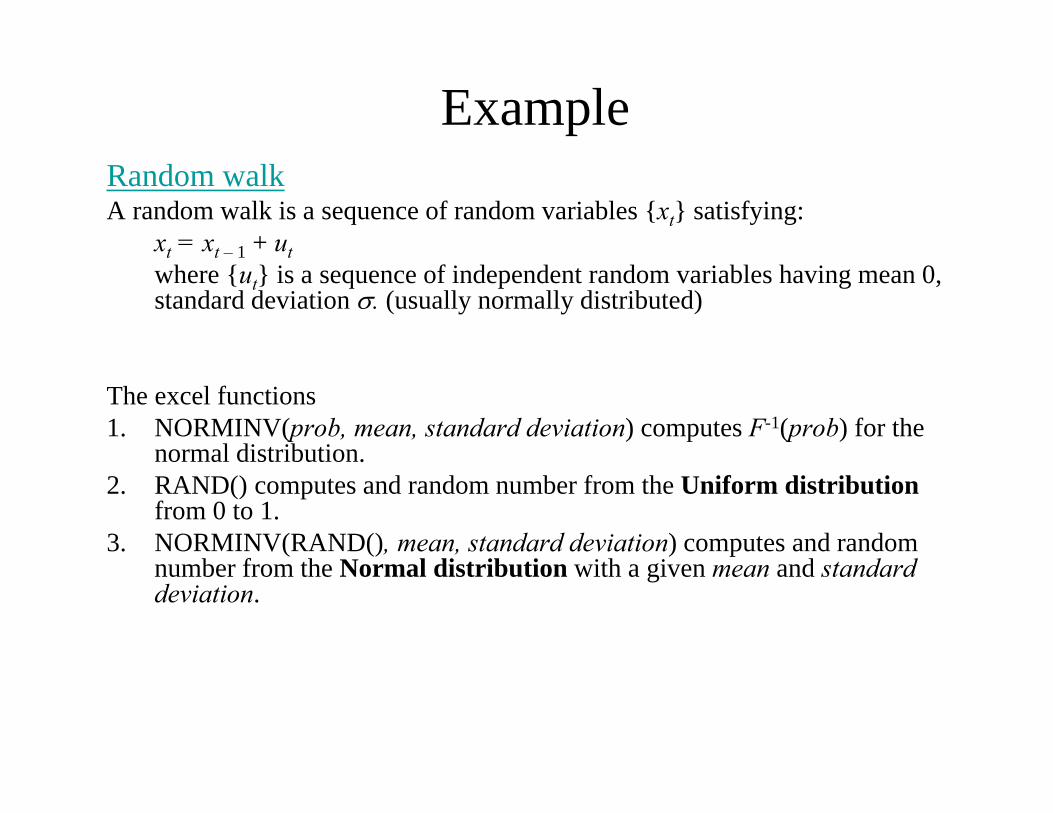
ExampleRandom walkA random walk is a sequence of random variables {xt} satisfying:

xt = xt – 1 + utwhere {ut} is a sequence of independent random variables having mean 0, standard deviation . (usually normally distributed)

The excel functions 1. NORMINV(prob, mean, standard deviation) computes F-1(prob) for the

normal distribution.2. RAND() computes and random number from the Uniform distribution

from 0 to 1.3. NORMINV(RAND(), mean, standard deviation) computes and random

number from the Normal distribution with a given mean and standard deviation.