Embed Size (px)
Citation preview
21 Statistics and Probability
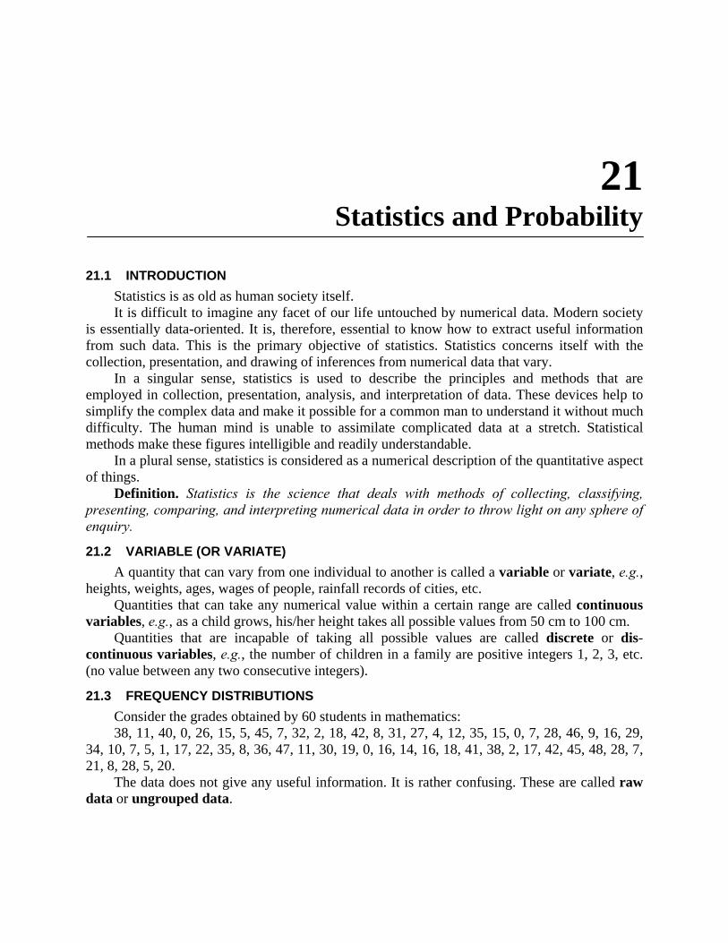
21.1 INTRODUCTION Statistics is as old as human society itself. It is difficult to imagine any facet of our life untouched by numerical data. Modern society
is essentially data-oriented. It is, therefore, essential to know how to extract useful information from such data. This is the primary objective of statistics. Statistics concerns itself with the collection, presentation, and drawing of inferences from numerical data that vary.
In a singular sense, statistics is used to describe the principles and methods that are employed in collection, presentation, analysis, and interpretation of data. These devices help to simplify the complex data and make it possible for a common man to understand it without much difficulty. The human mind is unable to assimilate complicated data at a stretch. Statistical methods make these figures intelligible and readily understandable.
In a plural sense, statistics is considered as a numerical description of the quantitative aspect of things.
Definition. Statistics is the science that deals with methods of collecting, classifying, presenting, comparing, and interpreting numerical data in order to throw light on any sphere of enquiry.
21.2 VARIABLE (OR VARIATE) A quantity that can vary from one individual to another is called a variable or variate, e.g.,
heights, weights, ages, wages of people, rainfall records of cities, etc. Quantities that can take any numerical value within a certain range are called continuous
variables, e.g., as a child grows, his/her height takes all possible values from 50 cm to 100 cm. Quantities that are incapable of taking all possible values are called discrete or dis-
continuous variables, e.g., the number of children in a family are positive integers 1, 2, 3, etc. (no value between any two consecutive integers).
21.3 FREQUENCY DISTRIBUTIONS Consider the grades obtained by 60 students in mathematics: 38, 11, 40, 0, 26, 15, 5, 45, 7, 32, 2, 18, 42, 8, 31, 27, 4, 12, 35, 15, 0, 7, 28, 46, 9, 16, 29,
34, 10, 7, 5, 1, 17, 22, 35, 8, 36, 47, 11, 30, 19, 0, 16, 14, 16, 18, 41, 38, 2, 17, 42, 45, 48, 28, 7, 21, 8, 28, 5, 20.
The data does not give any useful information. It is rather confusing. These are called raw data or ungrouped data.
1146 CHAPTER 21: STATISTICS AND PROBABILITY ________________________________________________________________________________________________________
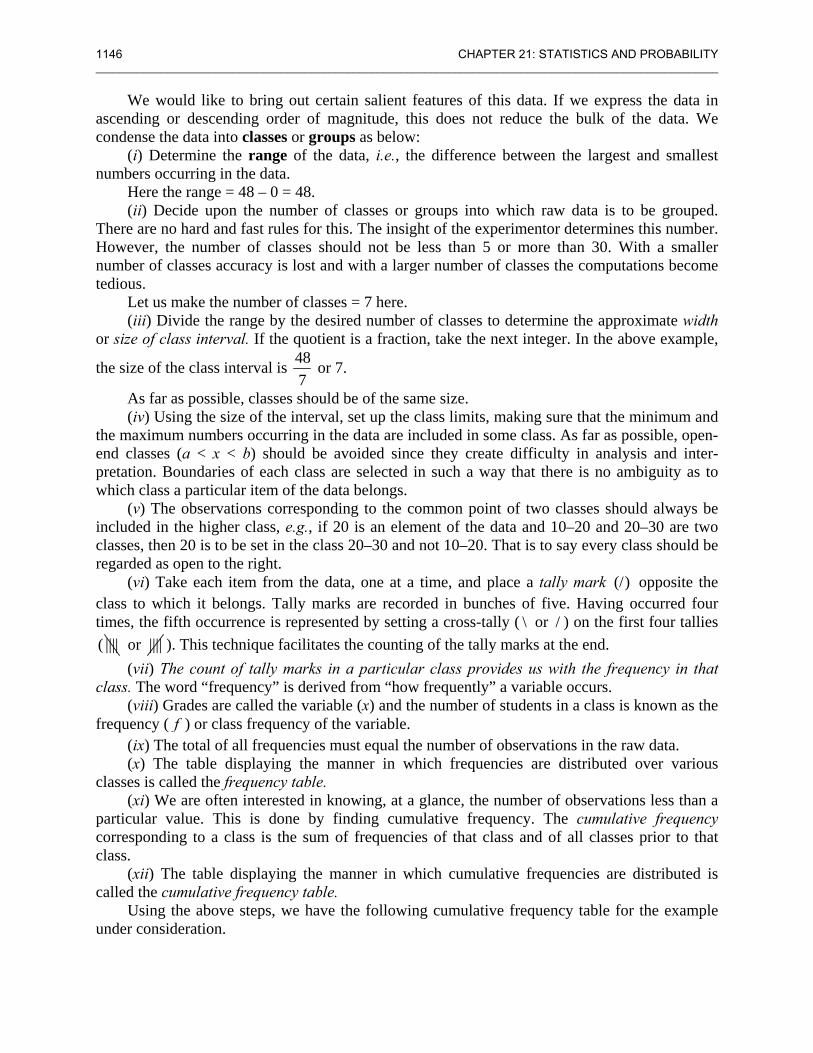
We would like to bring out certain salient features of this data. If we express the data in ascending or descending order of magnitude, this does not reduce the bulk of the data. We condense the data into classes or groups as below:
(i) Determine the range of the data, i.e., the difference between the largest and smallest numbers occurring in the data.
Here the range = 48 – 0 = 48. (ii) Decide upon the number of classes or groups into which raw data is to be grouped.
There are no hard and fast rules for this. The insight of the experimentor determines this number. However, the number of classes should not be less than 5 or more than 30. With a smaller number of classes accuracy is lost and with a larger number of classes the computations become tedious.
Let us make the number of classes = 7 here. (iii) Divide the range by the desired number of classes to determine the approximate width
or size of class interval. If the quotient is a fraction, take the next integer. In the above example,
the size of the class interval is 487
or 7.
As far as possible, classes should be of the same size. (iv) Using the size of the interval, set up the class limits, making sure that the minimum and
the maximum numbers occurring in the data are included in some class. As far as possible, open-end classes (a < x < b) should be avoided since they create difficulty in analysis and inter-pretation. Boundaries of each class are selected in such a way that there is no ambiguity as to which class a particular item of the data belongs.
(v) The observations corresponding to the common point of two classes should always be included in the higher class, e.g., if 20 is an element of the data and 10–20 and 20–30 are two classes, then 20 is to be set in the class 20–30 and not 10–20. That is to say every class should be regarded as open to the right.
(vi) Take each item from the data, one at a time, and place a tally mark (/) opposite the class to which it belongs. Tally marks are recorded in bunches of five. Having occurred four times, the fifth occurrence is represented by setting a cross-tally ( \ or / ) on the first four tallies ( |||| or |||| ). This technique facilitates the counting of the tally marks at the end.
(vii) The count of tally marks in a particular class provides us with the frequency in that class. The word “frequency” is derived from “how frequently” a variable occurs.
(viii) Grades are called the variable (x) and the number of students in a class is known as the frequency ( f ) or class frequency of the variable.
(ix) The total of all frequencies must equal the number of observations in the raw data. (x) The table displaying the manner in which frequencies are distributed over various
classes is called the frequency table. (xi) We are often interested in knowing, at a glance, the number of observations less than a
particular value. This is done by finding cumulative frequency. The cumulative frequency corresponding to a class is the sum of frequencies of that class and of all classes prior to that class.
(xii) The table displaying the manner in which cumulative frequencies are distributed is called the cumulative frequency table.
Using the above steps, we have the following cumulative frequency table for the example under consideration.
21.3 FREQUENCY DISTRIBUTIONS 1147 ________________________________________________________________________________________________________
Class interval Tally marks Frequency Cumulative (grades x) (number of students) ( f ) Frequency
0–7 |||| |||| 10 10 7–14 |||| |||| || 12 22
14–21 |||| |||| || 12 34 21–28 |||| 4 38 28–35 |||| ||| 8 46 35–42 |||| || 7 53 42–49 |||| || 7 60 Total 60
Example 1. The weights in grams of 50 apples picked at random from a market are as follows:
106, 107, 76, 82, 109, 107, 115, 93, 187, 195, 123, 125, 111, 92, 86, 70, 126, 68, 130, 129, 139, 119, 115, 128, 100, 186, 84, 99, 113, 204, 111, 141, 136, 123, 90, 115, 98, 110, 78, 90, 107, 81, 131, 75, 84, 104, 110, 80, 118, 82.
Form the grouped frequency table by dividing the variate range into intervals of equal width, each corresponding to 20 gms in such a way that the mid-value of the first class corresponds to 70 gms.
Sol. Mid-value of first class 70Width of each class 20
= ⎫⎬= ⎭
(given)
∴ The first class interval is (70 – 10) – (70 + 10) i.e., 60 – 80.
Weight in grams No. of apples Frequency
60–80 |||| 5 80–100 |||| |||| ||| 13
100–120 |||| |||| |||| || 17 120–140 |||| |||| 10 140–160 | 1 160–180 0 180–200 ||| 3 200–220 | 1
Total 50
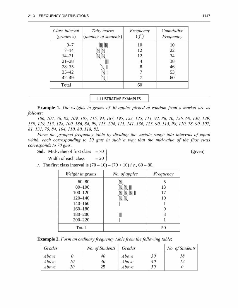
Example 2. Form an ordinary frequency table from the following table:
Grades No. of Students Grades No. of Students
Above 0 40 Above 30 18 Above 10 30 Above 40 12 Above 20 25 Above 50 0
ILLUSTRATIVE EXAMPLES
1148 __________
Sol.
Exa
G
B B B
Sol.
21.4 “E
Clasthe upper
______________
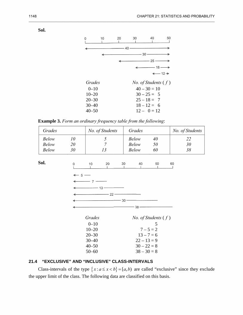
ample 3. For
Grades
Below Below Below
EXCLUSIVE
ss-intervals r limit of the
_____________
Gr 0–10–20–30–40–
rm an ordina
N
10 20 30
Gra 0–10–20–30–40–50–
E” AND “INC
of the type e class. The f
______________
rades–10–20–30–40–50
ary frequenc
No. of Studen
5 7 13
ades –10 –20 –30 –40 –50 –60
CLUSIVE” C
{ :x a x b≤ <following da
______________
No 4 3 2
cy table from
nts Gra
Belo Belo Belo
No
233
CLASS-INTE
} [ , )b a b= arata are classi
CHAPTER 21_____________
o. of Student40 – 30 = 1030 – 25 = 525 – 18 = 718 – 12 = 612 – 0 = 12
m the followin
des
ow 40 ow 50 ow 60
o. of Student5
7 – 5 = 2 13 – 7 = 6
22 – 13 = 9 30 – 22 = 8 38 – 30 = 8
ERVALS
re called “exified on this
: STATISTICS ______________
ts ( f ) 0 5 7 6 2
ng:
No. o
ts ( f )
xclusive” sinbasis.
AND PROBAB______________
of Students
22 30 38
nce they exc
BILITY ______
clude
21.5 THREE TYPES OF SERIES 1149 ________________________________________________________________________________________________________
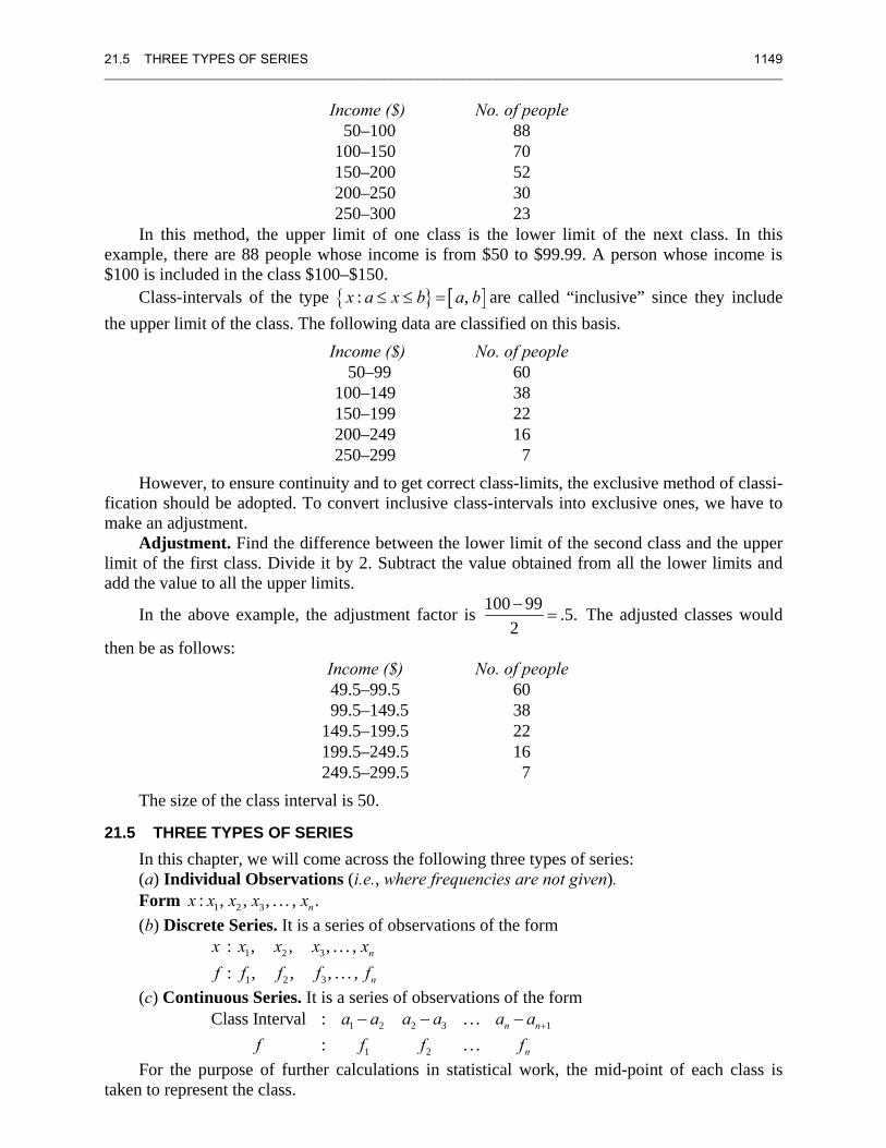
Income ($) No. of people 50–100 88 100–150 70 150–200 52 200–250 30 250–300 23
In this method, the upper limit of one class is the lower limit of the next class. In this example, there are 88 people whose income is from $50 to $99.99. A person whose income is $100 is included in the class $100–$150.
Class-intervals of the type { } [ ]: ,x a x b a b≤ ≤ = are called “inclusive” since they include the upper limit of the class. The following data are classified on this basis.
Income ($) No. of people 50–99 60 100–149 38 150–199 22 200–249 16 250–299 7
However, to ensure continuity and to get correct class-limits, the exclusive method of classi-fication should be adopted. To convert inclusive class-intervals into exclusive ones, we have to make an adjustment.
Adjustment. Find the difference between the lower limit of the second class and the upper limit of the first class. Divide it by 2. Subtract the value obtained from all the lower limits and add the value to all the upper limits.
In the above example, the adjustment factor is 100 99 .5.2−
= The adjusted classes would
then be as follows: Income ($) No. of people 49.5–99.5 60
99.5–149.5 38 149.5–199.5 22 199.5–249.5 16 249.5–299.5 7
The size of the class interval is 50.
21.5 THREE TYPES OF SERIES In this chapter, we will come across the following three types of series: (a) Individual Observations (i.e., where frequencies are not given). Form 1 2 3: , , , . . . , .nx x x x x (b) Discrete Series. It is a series of observations of the form
1 2 3
1 2 3
: , , , . . . ,: , , , . . . ,
n
n
x x x x xf f f f f
(c) Continuous Series. It is a series of observations of the form 1 2 2 3 1
1 2
Class Interval : . . .: . . .
n n
n
a a a a a af f f f
+− − −
For the purpose of further calculations in statistical work, the mid-point of each class is taken to represent the class.
1150 CHAPTER 21: STATISTICS AND PROBABILITY ________________________________________________________________________________________________________
Thus, if mi is the mid-point of the ith class, then mi = 1
2i ia a ++ and the above series takes the
The mid-value of the ith class may also be denoted by .ix Thus, a continuous series is reduced to the form of a discrete series. 21.6 GRAPHICAL REPRESENTATION
A frequency distribution when represented by means of a graph makes the unwieldy data intelligible. A better perspective can be had by representing the frequency distribution graphically since graphs, if drawn attractively, are eye-catching and leave a more lasting impression on the mind of the observer. Graphs are a good visual aid. But graphs do not give accurate measurements of the variable as are given by the tables. Another disadvantage is that by taking different scales, the facts may be misrepresented.
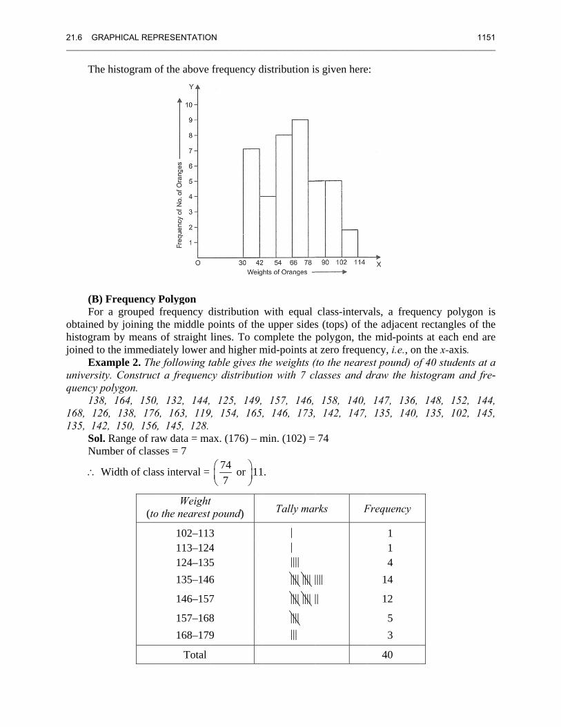
Some important types of graphs are given below: (A) Histogram In drawing the histogram of a given grouped frequency distribution: (a) Mark off along the x-axis all the class intervals on a suitable scale. (If class-intervals are
equal, then each = 1 cm is quite suitable.) (b) Mark frequencies along the y-axis on a suitable scale. (c) It must not be assumed that the scale for both the axes will be the same. We can have
different scales for the two axes. The determination of scale depends upon our convenience and the type and nature of the data. The scale or scales should be so chosen as to fit the size of graph-paper and to hold all the figures of the data.
(d) Construct rectangles with the class-intervals as bases and heights proportional (if the class intervals are equal) to the frequencies.
A diagram with all these rectangles is called a histogram.
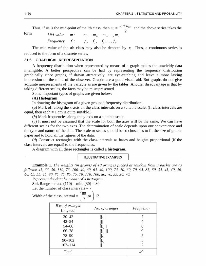
Example 1. The weights (in grams) of 40 oranges picked at random from a basket are as follows: 45, 55, 30, 110, 75, 100, 40, 60, 65, 40, 100, 75, 70, 60, 70, 95, 85, 80, 35, 45, 40, 50, 60, 65, 55, 45, 90, 85, 75, 85, 75, 70, 110, 100, 80, 70, 55, 30, 70.
Represent the data by means of a histogram. Sol. Range = max. (110) – min. (30) = 80 Let the number of class intervals = 7
Width of the class interval = 80 or7
⎛ ⎞⎜ ⎟⎝ ⎠
12.
Wts. of oranges No. of oranges Frequency (in gms.)
30–42 |||| || 7 42–54 |||| 4 54–66 |||| ||| 8 66–78 |||| |||| 9 78–90 |||| 5 90–102 |||| 5 102–114 || 2
Total 40
form
ILLUSTRATIVE EXAMPLES
1 2 3
1 2 3
- : , , , . . . ,: , , , . . . , .
n
n
Mid value m m m m mFrequency f f f f f
21.6 GRA__________
The
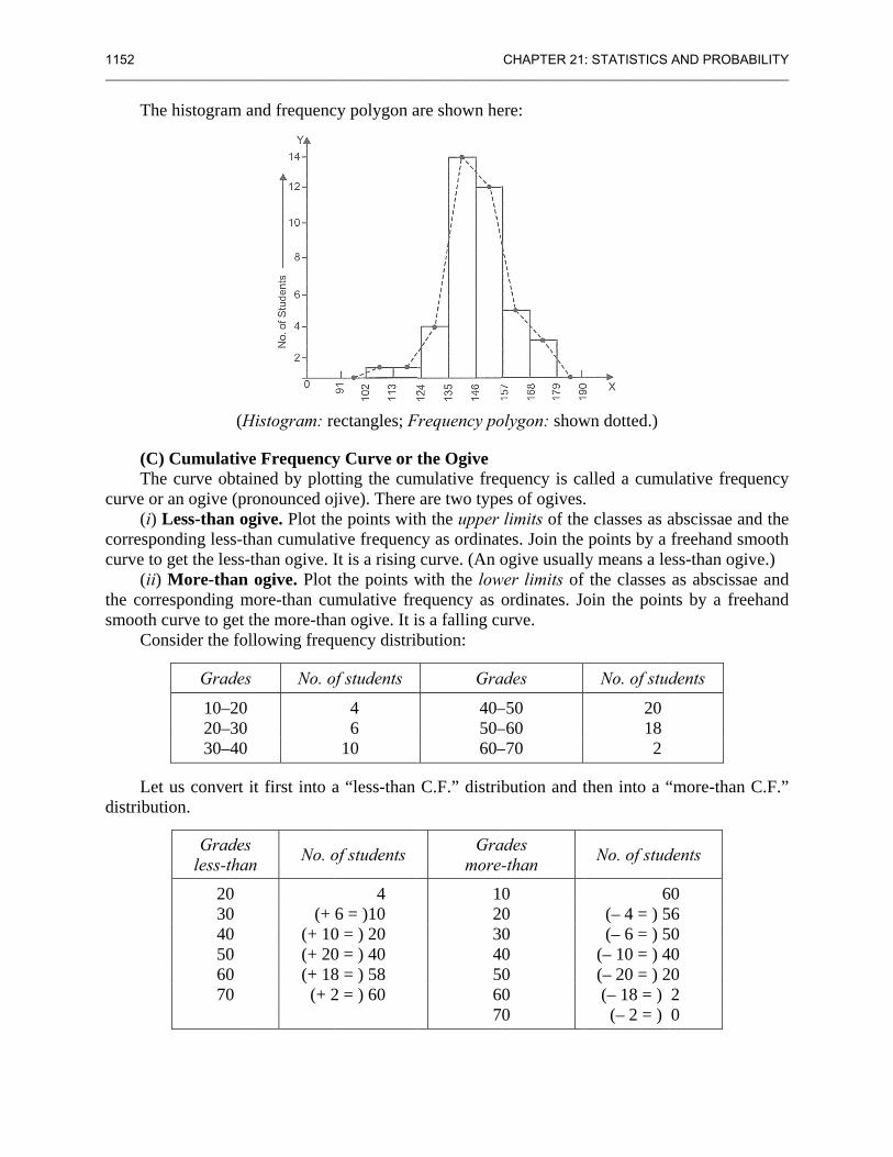
(B) For
obtained histogramjoined to
Exauniversityquency p
138,168, 126135, 142
Sol.Num
∴ W
APHICAL REP______________
histogram o
Frequency a grouped by joining t
m by means the immedi
ample 2. They. Construct
polygon. , 164, 150,6, 138, 1762, 150, 156, Range of ra
mber of class
Width of clas
(to
PRESENTATIO_____________
of the above
Polygon frequency dthe middle pof straight
ately lower e following tt a frequenc
, 132, 144,6, 163, 119, 145, 128. aw data = mases = 7
ss interval =
Weighto the nearest
102–113113–124124–135135–146
146–157
157–168168–179
Total
ON ______________
frequency d
distribution points of thelines. To coand higher mtable gives thcy distributio
125, 149,9, 154, 165,
ax. (176) – m
74 or 117
⎛ ⎞⎜ ⎟⎝ ⎠
t t pound)
3 4 5 6
7
8 9
______________
distribution i
with equal e upper sideomplete the mid-points athe weights (on with 7 c
157, 146, , 146, 173,
min. (102) =
.
Tally mar
| | |||| |||| ||||
|||| ||||
|||| |||
_____________
s given here
class-intervs (tops) of thpolygon, thet zero freque(to the nearelasses and d
158, 140, 142, 147,
74
rks F
||||
||
______________
e:
vals, a frequhe adjacent e mid-pointsency, i.e., onest pound) ofdraw the his
147, 136, 135, 140,
Frequency
1 1 4 14
12
5 3
40
______________
uency polygrectangles os at each en
n the x-axis. f 40 studentsstogram and
148, 152, 135, 102,
1151 ______
on is of the nd are
s at a d fre-
144, 145,
1152 __________
The
(C) The
curve or (i) L
corresponcurve to
(ii) the corresmooth c
Con
Let distributi
______________
histogram a
(H
Cumulative curve obtaian ogive (pr
Less-than ognding less-thget the less-tMore-than
esponding mcurve to get tnsider the fol
Grades
10–20 20–30 30–40
us convert iion.
Gradesless-than
20 30 40 50 60 70
_____________
and frequenc
Histogram: re
e Frequencyined by plotronounced ojgive. Plot thhan cumulatthan ogive. Iogive. Plot
more-than cuthe more-thallowing freq
s No. of
it first into a
s n No. o
(+ (+ 10(+ 20(+ 18
(+ 2
______________
cy polygon a
ectangles; F
y Curve or ttting the cumjive). There
he points witive frequencIt is a rising the points w
umulative frean ogive. It iuency distrib
of students
4 6 10
a “less-than
of students
4 6 = )10
0 = ) 20 0 = ) 40 8 = ) 58 2 = ) 60
______________
are shown he
Frequency po
the Ogive mulative freqare two type
th the upper cy as ordinatcurve. (An o
with the lowequency as is a falling cubution:
Gra
40–50–60–
C.F.” distrib
Gramore
1234567
CHAPTER 21_____________
ere:
olygon: show
quency is caes of ogives.limits of the
tes. Join the ogive usuall
wer limits of ordinates. Jourve.
ades
–50 –60 –70
bution and t
ades -than
0 0 0 0 0 0 0
: STATISTICS ______________
wn dotted.)
alled a cumu. e classes as apoints by a y means a le
f the classes oin the poin
No. of stu
20 18 2
then into a “
No. of stud
6(– 4 = ) 5(– 6 = ) 5
(– 10 = ) 4(– 20 = ) 2(– 18 = )
(– 2 = )
AND PROBAB______________
ulative frequ
abscissae anfreehand sm
ess-than ogivas abscissae
nts by a free
dents
“more-than C
dents
60 56 50 40 20
2 0
BILITY ______
uency
nd the mooth ve.) e and ehand
C.F.”
21.7 COM__________
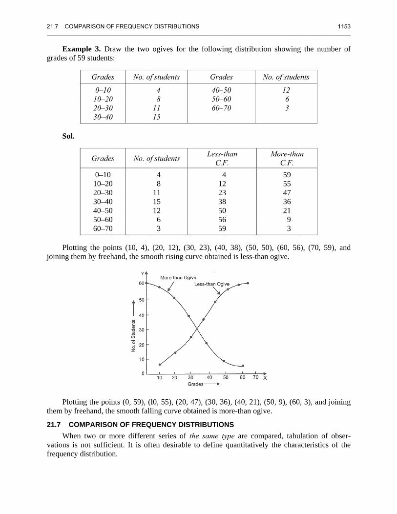
Exagrades of
Sol.
Plotjoining th
Plotthem by
21.7 COWhe
vations ifrequency
MPARISON OF______________
ample 3. Drf 59 students
Grades
0–10 10–2020–3030–40
Grades
0–10 10–2020–3030–4040–5050–6060–70
tting the poihem by freeh
tting the poinfreehand, th
OMPARISOen two or mis not sufficy distributio
F FREQUENC_____________
raw the twos:
s No. o
0 0 0
s No. o
0 0 0 0 0 0
ints (10, 4),hand, the sm
nts (0, 59), (e smooth fal
ON OF FREQmore differeient. It is of
on.
Y DISTRIBUTI______________
o ogives for
of students
4 8 11 15
of students
4 8 11 15 12 6 3
, (20, 12), (mooth rising c
(l0, 55), (20lling curve o
QUENCY DIent series offten desirabl
IONS______________
the followi
Grad
40–50–60–
Less-C.F 4122338505659
(30, 23), (40curve obtain
0, 47), (30, 3obtained is m
STRIBUTIOf the same tle to define
_____________
ing distribut
des
–50 –60 –70
-than F. 4 2 3 8 0 6 9
0, 38), (50, ned is less-th
36), (40, 21)more-than og
ONS type are com
quantitative
______________
tion showin
No. of stud
12 6 3
More-thaC.F. 59 55 47 36 21 9 3
50), (60, 56han ogive.
, (50, 9), (60give.
mpared, tabuely the char
______________
g the numb
dents
an
6), (70, 59)
0, 3), and jo
ulation of oracteristics o
1153 ______
ber of
, and
oining
obser-of the
1154 CHAPTER 21: STATISTICS AND PROBABILITY ________________________________________________________________________________________________________
There are two fundamental characteristics in which similar frequency distributions may differ:
(i) They may differ in measures of location or central tendency, i.e., in the value of the variate x around which they center.
(ii) They may differ in the extent to which observations are scattered about the central value. Measures of this kind are called measures of dispersion.
21.8 MEASURES OF CENTRAL TENDENCY Tabulation arranges facts in a logical order and helps their understanding and comparison.
But often, the groups tabulated are still too large for their characteristics to be readily grasped. What is desired is a numerical expression that summarizes the characteristic of the group. Measures of central tendency or measures of location (also popularly called averages) serve this purpose.
A figure that is used to represent a whole series should neither have the lowest value nor the highest in the series, but a value somewhere between these two limits, possibly in the center, where most of the items of the series cluster. Such figures are called Measures of Central Tendency (or averages).
There are five types of averages in common use:
1. Arithmetic Average or Mean 2. Median 3. Mode 4. Geometric Mean 5. Harmonic Mean
We shall take them one by one. 21.8.1 Arithmetic Mean
In the case of Individual Observations (i.e., where frequency is not given): 1. Direct Method. If 1 2: , , . . . , nx x x x then A.M. x is given by
1 2 . . . 1 .nx x xx xn n
+ + += = Σ
2. Short Cut Method. (Shift of origin.) Shifting the origin to an arbitrary point a, the formula
1 1becomes ( )x x x a x an n
= Σ − = Σ −
or 1 wherex xx a d d x an
= + Σ = −
Here, a = arbitrary number, called the Assumed Mean
1 2( ) ( ) ( ) . . . ( )
sum of the deviations of the variate from number of observations.
x nd x a x a x a x ax a
n
Σ = Σ − = − + − + + −==
In the case of a Discrete Series: 1. Direct Method. If the frequency distribution is
1 2
1 2
1 1 2 21 2
1 2
: , , . . . ,: , , . . . , , then
. . . where N . . .. . . N
n
n
n nn
n
x x x xf f f f
f x f x f x fxx f f f ff f f+ + + Σ
= = = + + + = Σ+ + +
21.8 MEASURES OF CENTRAL TENDENCY 1155 ________________________________________________________________________________________________________
2. Short Cut Method. (Shift of origin.) Shifting the origin to an arbitrary point a, the formula
1 1becomes ( )N N
x fx x a f x a= Σ − = Σ −
or 1 , whereN x xx a fd d x a= + Σ = −
Thus where assumed meanx a a= + Σ =x1 fdN
1 1 2 2
1 2
( )( ) ( ) . . . ( )
sum of the products of and the deviation of the corresponding variate from .N . . . .
x
n n
n
fd f x af x a f x a f x a
f x af f f f
Σ = Σ −= − + − + + −== + + + = Σ
Note. If the frequencies are given in terms of class intervals, the mid-values of the class intervals are considered as x and then the above formulae are applied.
In the case of Continuous Series having equal class intervals, say of width h, we use a different formula (Shift of origin and change of scale; Step Deviation Method).
Let thenx au x a huh−
= = +
∴ ( )fx f a hu a f h fuΣ = Σ + = Σ + Σ
Dividing both sides by N ,f= Σ we get
or where .N Nfx h fu x aa x a u
hΣ Σ Σ −
= + = + =fuhN
Weighted Arithmetic Mean. If the variate-values are not of equal importance, we may attach weights to them 1 2, , . . . , nw w w as measures of their importance.
The weighted mean wx is defined as 1 1 2 2
1 2
. . .. . .
n nw
n
w x w x w x wxxw w w w
+ + + Σ= =
+ + + Σ (i.e., write w for f ).
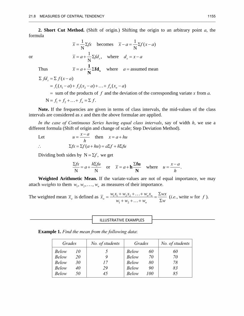
Example 1. Find the mean from the following data:
Grades No. of students Grades No. of students
Below 10 5 Below 60 60 Below 20 9 Below 70 70 Below 30 17 Below 80 78 Below 40 29 Below 90 83 Below 50 45 Below 100 85
ILLUSTRATIVE EXAMPLES
1156 CHAPTER 21: STATISTICS AND PROBABILITY ________________________________________________________________________________________________________
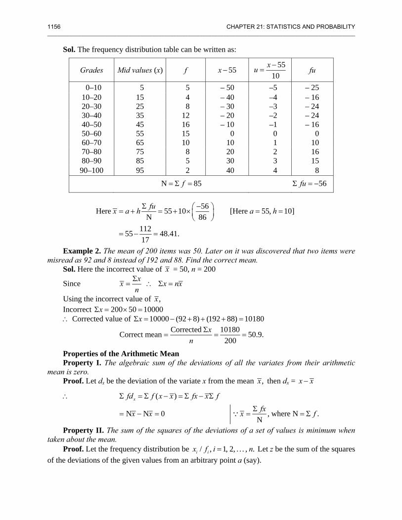
Sol. The frequency distribution table can be written as:
Grades Mid values (x) f 55x − 55
10xu −
= fu
0–10 5 5 – 50 –5 – 25 10–20 15 4 – 40 –4 – 16 20–30 25 8 – 30 –3 – 24 30–40 35 12 – 20 –2 – 24 40–50 45 16 – 10 –1 – 16 50–60 55 15 0 0 0 60–70 65 10 10 1 10 70–80 75 8 20 2 16 80–90 85 5 30 3 15 90–100 95 2 40 4 8
N 85f= Σ = 56fuΣ = −
56Here 55 10 [Here 55, 10]N 86
11255 48.41.17
fux a h a hΣ −⎛ ⎞= + = + × = =⎜ ⎟⎝ ⎠
= − =
Example 2. The mean of 200 items was 50. Later on it was discovered that two items were misread as 92 and 8 instead of 192 and 88. Find the correct mean.
Sol. Here the incorrect value of x = 50, n = 200
Since xx x nxn
Σ= ∴ Σ =
Using the incorrect value of ,x Incorrect 200 50 10000xΣ = × = ∴ Corrected value of 10000 (92 8) (192 88) 10180xΣ = − + + + =
Corrected 10180Correct mean 50.9.200
xn
Σ= = =
Properties of the Arithmetic Mean Property I. The algebraic sum of the deviations of all the variates from their arithmetic
mean is zero. Proof. Let dx be the deviation of the variate x from the mean ,x then dx = x x−
∴ ( )
N N 0 , where N .N
xfd f x x fx x ffxx x x f
Σ = Σ − = Σ − Σ
Σ= − = = = Σ∵
Property II. The sum of the squares of the deviations of a set of values is minimum when taken about the mean.
Proof. Let the frequency distribution be / , 1, 2, . . . , .i ix f i n= Let z be the sum of the squares of the deviations of the given values from an arbitrary point a (say).
21.8 MEASURES OF CENTRAL TENDENCY 1157 ________________________________________________________________________________________________________
⇒ Let 2
1( ) .
n
iz f x a
=
= −∑
We have to show that z is minimum when .a x=
z will be minimum when 0dzda
= and 2
2 0d zda
>
Now 1 12 ( ) ( 1) 2 ( )
n n
i i
dz f x a f x ada = =
= − ⋅ − = − −∑ ∑
0 2 ( ) 0
0N N 0
0
dz f x ada
fx a fx a
x aa x
∴ = ⇒ − Σ − =
⇒ Σ − Σ =⇒ − =⇒ − =⇒ =
, NN
( N 0)
fxx f
f
Σ⎡ ⎤= Σ =⎢ ⎥⎣ ⎦= Σ ≠
∵
∵
Also 2
21
2 ( 1) 2 2N 0n
i
d z f fda =
= − − = Σ = >∑
Hence z is minimum when .a x= Property III. (Mean of the composite series.) If ix (i = 1, 2, . . . , k) are the arithmetic means of k distributions with respective fre-
quencies ni (i = 1, 2, . . . , k), then the mean x of the whole distribution obtained by combining the k distributions is given by
1 1 2 2
1 2
......
i ik k i
k ii
n xn x n x n xxn n n n
Σ+ + += =
+ + + Σ
Proof. Let 111 12 13 1, , , . . . , nx x x x be the variables of the first distribution, 21,x 22 ,x . . . ,
22nx be the variables of the second distribution, and so on. Then by definition
1
2
1 2
1 11 12 11
2 21 22 22
1 ( . . . )
1 ( . . . ). . . ( )
.............................................1 ( . . . )
k
n
n
n k k knk
x x x xn
x x x xn A
x x x xn
⎫= + + + ⎪⎪⎪= + + + ⎪⎬⎪⎪⎪= + + + ⎪⎭
The mean x of the whole distribution of size 1 2( . . . )kn n n+ + + is given by
1 2 1 211 12 1 21 22 2
1 2
1 1 2 2
1 2
( . . . ) ( . . . ) . . . ( . . . ). . .
. . .. . .
kn n k k kn
k
i ik k i
k ii
x x x x x x x x xx
n n nn xn x n x n xk
n n n n
+ + + + + + + + + + + +=
+ + +
Σ+ + += =
+ + + Σ
1158 CHAPTER 21: STATISTICS AND PROBABILITY ________________________________________________________________________________________________________
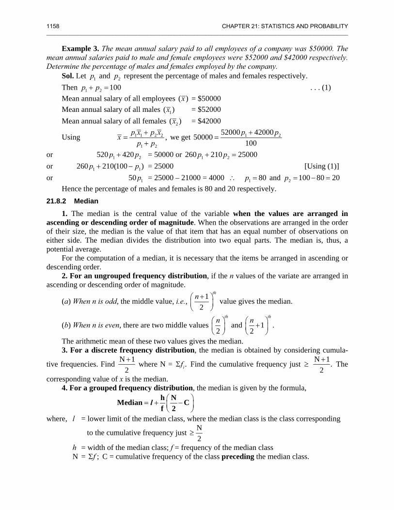
Example 3. The mean annual salary paid to all employees of a company was $50000. The mean annual salaries paid to male and female employees were $52000 and $42000 respectively. Determine the percentage of males and females employed by the company.
Sol. Let 1p and 2p represent the percentage of males and females respectively. Then 1 2 100p p+ = . . . (1) Mean annual salary of all employees ( )x = $50000 Mean annual salary of all males 1( )x = $52000 Mean annual salary of all females 2( )x = $42000
Using 1 1 2 2
1 2
,p x p xxp p
+=
+ we get 1 252000 4200050000
100p p+
=
or 1 2520 420p p+ = 50000 or 1 2260 210 25000p p+ = or 1 1260 210(100 )p p+ − = 25000 [Using (1)] or 150 p = 25000 – 21000 = 4000 ∴ 1 80p = and 2 100 80 20p = − =
Hence the percentage of males and females is 80 and 20 respectively. 21.8.2 Median
1. The median is the central value of the variable when the values are arranged in ascending or descending order of magnitude. When the observations are arranged in the order of their size, the median is the value of that item that has an equal number of observations on either side. The median divides the distribution into two equal parts. The median is, thus, a potential average.
For the computation of a median, it is necessary that the items be arranged in ascending or descending order.
2. For an ungrouped frequency distribution, if the n values of the variate are arranged in ascending or descending order of magnitude.
(a) When n is odd, the middle value, i.e., 12
thn +⎛ ⎞⎜ ⎟⎝ ⎠
value gives the median.
(b) When n is even, there are two middle values 2
thn⎛ ⎞⎜ ⎟⎝ ⎠
and 1 .2
thn⎛ ⎞+⎜ ⎟⎝ ⎠
The arithmetic mean of these two values gives the median. 3. For a discrete frequency distribution, the median is obtained by considering cumula-
tive frequencies. Find N 12+ where N = .ifΣ Find the cumulative frequency just ≥ N 1.
2+ The
corresponding value of x is the median. 4. For a grouped frequency distribution, the median is given by the formula,
⎛ ⎞= + −⎜ ⎟⎝ ⎠
h NMedian Cf 2
l
where, l = lower limit of the median class, where the median class is the class corresponding
to the cumulative frequency just N2
≥
h = width of the median class; f = frequency of the median class N = ;fΣ C = cumulative frequency of the class preceding the median class.
21.8 MEASURES OF CENTRAL TENDENCY 1159 ________________________________________________________________________________________________________
5. Partition values. These are the values of the variate that divide the total frequency into a number of equal parts, the median being that value of the variate that divides the total frequency into two equal parts.
(a) Quartiles. Quartiles are those values of the variate that divide the total frequency into four equal parts. When the lower half before the median is divided into two equal parts, the value of the dividing variate is called the Lower Quartile and is denoted by Q1. The value of the variate dividing the upper half into two equal parts is called the Upper Quartile and is denoted by Q3. (Q2 being the median.) The formulae for computation are
1 3N 3NQ C ; Q C4 4
h hl lf f
⎛ ⎞ ⎛ ⎞= + − = + −⎜ ⎟ ⎜ ⎟⎝ ⎠ ⎝ ⎠
(b) Deciles. Deciles are those values of the variate that divide the total frequency into 10 equal parts. D1, D2, . . . denote respectively the first, second, . . . deciles.
1 4 7N 4N 7ND C , D C , D C10 10 10
h h hl l lf f f
⎛ ⎞ ⎛ ⎞ ⎛ ⎞= + − = + − = + −⎜ ⎟ ⎜ ⎟ ⎜ ⎟⎝ ⎠ ⎝ ⎠ ⎝ ⎠
(The fifth decile D5 is the median.)
(c) Percentiles. Percentiles are those values of the variate that divide the total frequency into 100 equal parts. If P1, P2, . . . denote respectively the first, second, . . . percentiles, then
9 729N 72NP C , P C etc.100 100
h hl lf f
⎛ ⎞ ⎛ ⎞= + − = + −⎜ ⎟ ⎜ ⎟⎝ ⎠ ⎝ ⎠
(The 50th percentile P50 is the median.)
In the above formulae for Quartiles, Deciles, and Percentiles, the letters l, i, f, N, C have been used in the same sense in which they have been used in the formula for the median.
Example 1. Below are given the grades obtained by a group of 20 students in a certain class in mathematics and physics:
Roll Nos. : 1 2 3 4 5 6 7 8 9 10 Grades in Math : 53 54 52 32 30 60 47 46 35 28 Grades in Physics : 58 55 25 32 26 85 44 80 33 72 Roll Nos. : 11 12 13 14 15 16 17 18 19 20 Grades in Math : 25 42 33 48 72 51 45 33 65 29 Grades in Physics : 10 42 15 46 50 64 39 38 30 36
In which subject is the level of knowledge of the students higher?
Sol. To find out the subject in which the level of knowledge of the students is higher, we find out the medians of both the series. The subject for which the median value is higher will be the subject in which the level of knowledge of the students is higher. Let us arrange the grades in ascending order of magnitude.
ILLUSTRATIVE EXAMPLES
1160 CHAPTER 21: STATISTICS AND PROBABILITY ________________________________________________________________________________________________________
S. No. Grades in Math
Grades in Physics S. No. Grades in
Math Grades in Physics
1 25 10 11 46 42 2 28 15 12 47 44 3 29 25 13 48 46 4 30 26 14 51 50 5 32 30 15 52 55 6 33 32 16 53 58 7 33 33 17 54 64 8 35 36 18 60 72 9 42 38 19 65 80 10 45 39 20 72 85
Number of items in each case = 20 (even) Median grades in Mathematics
= A.M. of sizes of 20 th2
⎛ ⎞⎜ ⎟⎝ ⎠
and 20 1 th2
⎛ ⎞+⎜ ⎟⎝ ⎠
items
= A.M. of sizes of 10th and 11th items = 45 462+ = 45.5.
Median grades in physics = A.M. of sizes of 10th and 11th items = 39 422+ = 40.5.
Since the median grades in mathematics are greater than the median grades in physics, the level of knowledge in mathematics is higher.
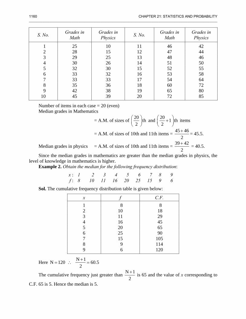
Example 2. Obtain the median for the following frequency distribution:
x : 1 2 3 4 5 6 7 8 9 f : 8 10 11 16 20 25 15 9 6
Sol. The cumulative frequency distribution table is given below:
x f C.F. 1 8 8 2 10 18 3 11 29 4 16 45 5 20 65 6 25 90 7 15 105 8 9 114 9 6 120
Here N 1N 120 60.52+
= ∴ =
The cumulative frequency just greater than N 12+ is 65 and the value of x corresponding to
C.F. 65 is 5. Hence the median is 5.
21.8 MEASURES OF CENTRAL TENDENCY 1161 ________________________________________________________________________________________________________
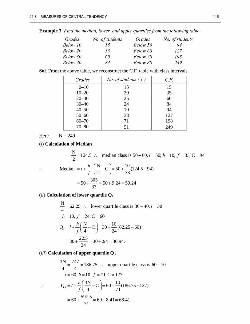
Example 3. Find the median, lower, and upper quartiles from the following table:
Grades No. of students Grades No. of students Below 10 15 Below 50 94 Below 20 35 Below 60 127 Below 30 60 Below 70 198 Below 40 84 Below 80 249
Sol. From the above table, we reconstruct the C.F. table with class intervals.
Grades No. of students ( f ) C.F. 0–10 15 15 10–20 20 35 20–30 25 60 30–40 24 84 40–50 10 94 50–60 33 127 60–70 71 198 70–80 51 249
Here N = 249
(i) Calculation of Median
∴
N 124.5 median class is 50 60, 50; 10, 33, C 942
N 10Median C 50 (124.5 94)2 33
30550 50 9.24 59.2433
l h f
hlf
= ∴ − = = = =
⎛ ⎞= + − = + −⎜ ⎟⎝ ⎠
= + = + =
(ii) Calculation of lower quartile Q1
1
N 62.25 lower quartile class is 30 40, 304
10, 24, C 60N 10Q C 30 (62.25 60)4 24
22.530 30 .94 30.94.24
l
h fhlf
= ∴ − =
= = =
⎛ ⎞= + − = + −⎜ ⎟⎝ ⎠
= + = + =
(iii) Calculation of upper quartile Q3
3
3N 747 186.75 upper quartile class is 60 704 4
60, 10, 71, C 1273N 10Q C 60 (186.75 127)4 71
597.560 60 8.41 68.41.71
l h fhlf
= = ∴ −
= = = =
⎛ ⎞= + − = + −⎜ ⎟⎝ ⎠
= + = + =
∴
∴
1162 CHAPTER 21: STATISTICS AND PROBABILITY ________________________________________________________________________________________________________
21.8.3 Mode
1. Mode. Mode is the value that occurs most frequently in a set of observations and around which the other items of the set cluster densely. It is the point of maximum frequency or the point of greatest density. In other words, the mode or modal value of the distribution is that value of the variate for which frequency is maximum.
2. Calculation of the Mode. (a) In the case of discrete frequency distribution, mode is the value of x corresponding to
maximum frequency. But in any one (or more) of the following cases: (i) if the maximum frequency is repeated (ii) if the maximum frequency occurs in the very beginning or at the end of the distribution (iii) if there are irregularities in the distribution, the value of the mode is determined by the
method of grouping (illustrated in the examples below). (b) In the case of a continuous frequency distribution, the mode is given by the formula:
1
1 2
Mode2
m
m
f fl hf f f
−= + ×
− −
where l is the lower limit, h is the width, and fm is the frequency of the model class, and f1 and f2 are the frequencies of the classes preceding and succeeding the modal class respectively.
While applying the above formula, it is necessary to see that the class-intervals are of the same size. If they are unequal, they should first be made equal on the assumption that the frequencies are equally distributed throughout the class.
In case fm – f1 < 0 or 2fm – f1 – f2 = 0, use the formula
1
1 2
Mode l hΔ= + ×
Δ + Δ
where 1 1 2 2and .m mf f f fΔ = − Δ = − (c) For a symmetrical distribution, the mean, median, and mode coincide. (d) Where the mode is ill-defined, i.e., where the method of grouping also fails, its value
can be ascertained by the formula
Mode = 3 Median – 2 Mean This measure is called the empirical mode.
Example 1. Calculate the mode from the following frequency distribution:
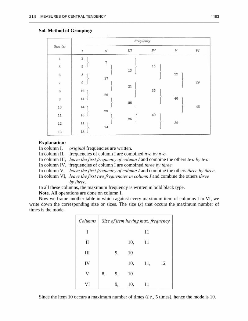
Size (x) : 4 5 6 7 8 9 10 11 12 13 Frequency ( f ) : 2 5 8 9 12 14 14 15 11 13
ILLUSTRATIVE EXAMPLES
21.8 MEA__________
Sol.
ExpIn cIn cIn cIn cIn cIn c
In aNotNow
write dowtimes is t
Sinc
ASURES OF C______________
Method of
planation: olumn I, oolumn II, folumn III, lolumn IV, folumn V, lolumn VI, l
bll these colue. All operat
w we frame wn the correthe mode.
ce the item 1
CENTRAL TEN_____________
f Grouping:
original freqfrequencies leave the firsfrequencies leave the firsleave the firsby three.
umns, the mations are donanother tablesponding s
Column
I
II
III
IV
V
VI
10 occurs a m
NDENCY______________
quencies are of column I st frequencyof column I st frequencyst two freque
aximum freqne on columle in which asize or sizes
ns Size of
9
8, 9
9
maximum nu
______________
written. are combine
y of column Iare combine
y of column Iencies in col
quency is wrimn I.
against every. The size (
item having
10,
9, 10
10,
9, 10
9, 10,
umber of tim
_____________
ed two by twI and combined three by tI and combinlumn I and c
itten in bold
y maximum (x) that occu
max. freque
11
11
11, 1
11
mes (i.e., 5 tim
______________
wo. ne the othersthree. ne the otherscombine the
black type.
item of coluurs the maxi
ency
12
mes), hence
______________
s two by two.
s three by throthers three
umns I to Vimum numb
the mode is
1163 ______
.
ree. e
VI, we ber of
10.
1164 CHAPTER 21: STATISTICS AND PROBABILITY ________________________________________________________________________________________________________
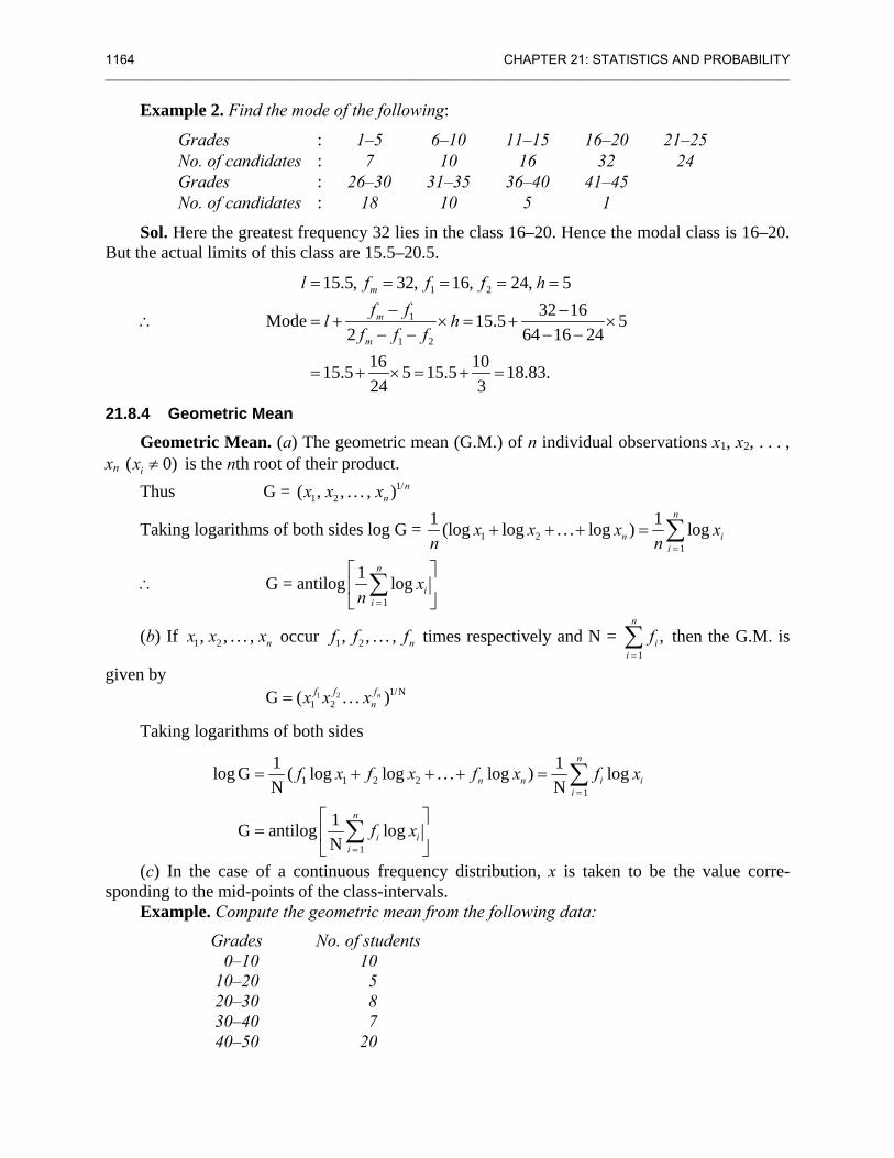
Example 2. Find the mode of the following:
Grades : 1–5 6–10 11–15 16–20 21–25 No. of candidates : 7 10 16 32 24 Grades : 26–30 31–35 36–40 41–45 No. of candidates : 18 10 5 1
Sol. Here the greatest frequency 32 lies in the class 16–20. Hence the modal class is 16–20. But the actual limits of this class are 15.5–20.5.
∴
1 2
1
1 2
15.5, 32, 16, 24, 532 16Mode 15.5 5
2 64 16 2416 1015.5 5 15.5 18.83.24 3
m
m
m
l f f f hf fl h
f f f
= = = = =− −
= + × = + ×− − − −
= + × = + =
21.8.4 Geometric Mean
Geometric Mean. (a) The geometric mean (G.M.) of n individual observations x1, x2, . . . , xn ( 0)ix ≠ is the nth root of their product.
Thus G = 1/1 2( , , . . . , ) n
nx x x
Taking logarithms of both sides log G = 1 21
1 1(log log . . . log ) logn
n ii
x x x xn n =
+ + + = ∑
∴ 1
1G = antilog logn
ii
xn =
⎡ ⎤⎢ ⎥⎣ ⎦
∑
(b) If 1 2, , . . . , nx x x occur 1 2, , . . . , nf f f times respectively and N = 1
,n
ii
f=∑ then the G.M. is
given by 1 2 1/N
1 2G ( . . . )nff fnx x x=
Taking logarithms of both sides
1 1 2 2
1
1
1 1log G ( log log . . . log ) logN N
1G antilog logN
n
n n i ii
n
i ii
f x f x f x f x
f x
=
=
= + + + =
⎡ ⎤= ⎢ ⎥
⎣ ⎦
∑
∑
(c) In the case of a continuous frequency distribution, x is taken to be the value corre-sponding to the mid-points of the class-intervals.
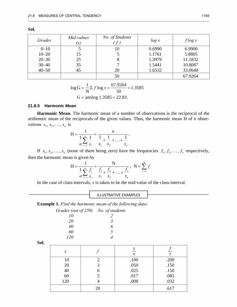
Example. Compute the geometric mean from the following data:
Grades No. of students 0–10 10 10–20 5 20–30 8 30–40 7 40–50 20
21.8 MEASURES OF CENTRAL TENDENCY 1165 ________________________________________________________________________________________________________
Sol.
Grades Mid-values (x)
No. of Students ( f ) log x f log x
0–10 5 10 0.6990 6.9900 10–20 15 5 1.1761 5.8805 20–30 25 8 1.3979 11.1832 30–40 35 7 1.5441 10.8087 40–50 45 20 1.6532 33.0640
50 67.9264
1 67.9264log G log 1.3585N 50
G antilog 1.3585 22.83.
f x= Σ = =
= =
21.8.5 Harmonic Mean
Harmonic Mean. The harmonic mean of a number of observations is the reciprocal of the arithmetic mean of the reciprocals of the given values. Thus, the harmonic mean H of n obser-vations 1 2, , . . . , nx x x is
1 1 2
1H .1 1 11 1 . . .n
i ni
n
x x xn x=
= =+ + +∑
If 1 2, , . . . , nx x x (none of them being zero) have the frequencies 1 2, , . . . , nf f f respectively, then the harmonic mean is given by
1 2 1
1 1 2
1 NH , N1 . . .
n
inn ii
i ni
fff ffx x xn x
=
=
= = =+ + +
∑∑
In the case of class-intervals, x is taken to be the mid-value of the class-interval.
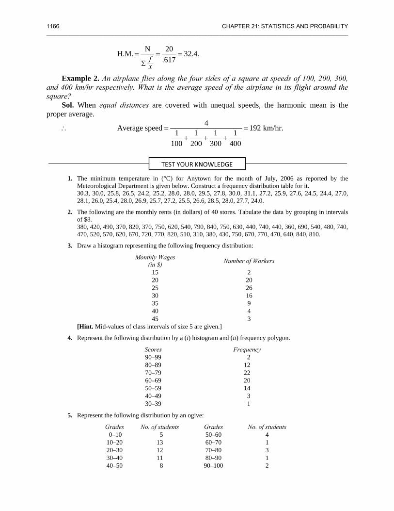
Example 1. Find the harmonic mean of the following data: Grades (out of 150) No. of students
10 2 20 3 40 6 60 5 120 4 Sol.
x f 1x f
x
10 2 .100 .200 20 3 .050 .150 40 6 .025 .150 60 5 .017 .085 120 4 .008 .032
20 .617
ILLUSTRATIVE EXAMPLES
1166 CHAPTER 21: STATISTICS AND PROBABILITY ________________________________________________________________________________________________________
N 20H.M. 32.4..617f
x= = =
Σ
Example 2. An airplane flies along the four sides of a square at speeds of 100, 200, 300, and 400 km/hr respectively. What is the average speed of the airplane in its flight around the square?
Sol. When equal distances are covered with unequal speeds, the harmonic mean is the proper average.
∴ 4Average speed 192 km/hr.1 1 1 1100 200 300 400
= =+ + +
1. The minimum temperature in (°C) for Anytown for the month of July, 2006 as reported by the Meteorological Department is given below. Construct a frequency distribution table for it.
30.3, 30.0, 25.8, 26.5, 24.2, 25.2, 28.0, 28.0, 29.5, 27.8, 30.0, 31.1, 27.2, 25.9, 27.6, 24.5, 24.4, 27.0, 28.1, 26.0, 25.4, 28.0, 26.9, 25.7, 27.2, 25.5, 26.6, 28.5, 28.0, 27.7, 24.0.
2. The following are the monthly rents (in dollars) of 40 stores. Tabulate the data by grouping in intervals of $8.
380, 420, 490, 370, 820, 370, 750, 620, 540, 790, 840, 750, 630, 440, 740, 440, 360, 690, 540, 480, 740, 470, 520, 570, 620, 670, 720, 770, 820, 510, 310, 380, 430, 750, 670, 770, 470, 640, 840, 810.
3. Draw a histogram representing the following frequency distribution:
Monthly Wages (in $) Number of Workers
15 2 20 20 25 26 30 16 35 9 40 4 45 3
[Hint. Mid-values of class intervals of size 5 are given.]
4. Represent the following distribution by a (i) histogram and (ii) frequency polygon.
Scores Frequency 90–99 2 80–89 12 70–79 22 60–69 20 50–59 14 40–49 3 30–39 1
5. Represent the following distribution by an ogive:
Grades No. of students Grades No. of students 0–10 5 50–60 4 10–20 13 60–70 1 20–30 12 70–80 3 30–40 11 80–90 1 40–50 8 90–100 2
TEST YOUR KNOWLEDGE
21.8 MEASURES OF CENTRAL TENDENCY 1167 ________________________________________________________________________________________________________
6. Compute the arithmetic mean for the following data:
Height (in cm): 219 216 213 210 207 204 201 198 195 No. of people: 2 4 6 10 11 7 5 4 1
7. Find the average grades of students from the following data:
Grades No. of students Grades No. of students Above 0 80 Above 60 28
Above 10 77 Above 70 16 Above 20 72 Above 80 10 Above 30 65 Above 90 8 Above 40 55 Above 100 0 Above 50 43
8. Two hundred people were interviewed by a public opinion polling agency. The frequency distribution gives the ages of the people interviewed.
Age Group Frequency Age Group Frequency 80–89 2 40–49 56 70–79 2 30–39 40 60–69 6 20–29 42 50–59 20 10–19 32
Calculate the arithmetic mean of the data.
9. Calculate the arithmetic mean from the following data:
Class interval Frequency Class interval Frequency 0–1 8 15–25 11 1–3 8 25–28 10 3–5 10 28–30 9
5–10 12 30–45 8 10–15 18 45–60 6
10. Find the class intervals if the arithmetic mean of the following distribution is 33 and assumed mean is 35.
Step deviation (u) : – 3 – 2 – 1 0 1 2 Frequency ( f ) : 5 10 25 30 20 10
11. The average height of a group of 25 children was calculated to be 78.4 cm. It was later discovered that one value was misread as 69 cm instead of the correct value of 96 cm. Calculate the correct average.
12. A candidate obtains the following percentage in an examination: english 60, history 75, mathematics 63, physics 59, and chemistry 55. Find the weighted mean if weights 2, 1, 5, 5, 3 are allotted to the subjects.
13. From the following data calculate the missing frequency:
No. of pills No. of people cured No. of pills No. of people cured 4–8 11 24–28 9
8–12 13 28–32 17 12–16 16 32–36 6 16–20 14 36–40 4 20–24 ?
The average number of pills to cure a person is 20.
14. The frequencies of values 0, 1, 2, . . . , n of a variable are given by
qn, nC1qn–lp, nC2qn–2p2, . . . , pn where p + q = 1. Show that the mean is np.
1168 CHAPTER 21: STATISTICS AND PROBABILITY ________________________________________________________________________________________________________
15. The mean grades obtained by 300 students in the subject of statistics is 45. The mean of the top 100 of them was found to be 70 and the mean of the last 100 was known to be 20. What is the mean of the remaining 100 students?
16. In a certain examination, the average grade of all students in class A is 68.4 and that of all students in class B is 71.2. If the average of both classes combined is 70, find the ratio of the number of students in class A to the number in class B.
17. The following are the monthly salaries in dollars of 30 employees of a firm:
910 1390 1260 1190 1000 870 650 770 990 950 1080 1270 860 1480 1160 760 690 880 1120 1180 890 1160 970 1050 950 800 860 1060 930 1350
The firm gave bonuses of 100, 150, 200, 250, 300, 350, 400, 450, and 500 to employees in the respective salary groups: exceeding 600 but not exceeding 700, exceeding 700 but not exceeding 800, and so on up to exceeding 1400 but not exceeding 1500. Find the average bonus paid per employee.
18. According to the census of 2006, the following are the population figures in thousands of 10 cities:
2000, 1180, 1785, 1500, 560, 782, 1200, 385, 1123, 222. Find the median.
19. Find the median from the following table:
x : 5 7 9 11 13 15 17 19 f : 1 2 7 9 11 8 5 4
20. Calculate the mean and median from the following table:
Class interval Frequency 6.5–7.5 5 7.5–8.5 12 8.5–9.5 25
9.5–10.5 48 10.5–11.5 32 11.5–12.5 6 12.5–13.5 1
21. Compute the median from the following data:
Mid-value Frequency Mid-value Frequency 115 6 165 60 125 25 175 38 135 48 185 22 145 72 195 3 155 116
22. Find the median, quartiles, 7th decile, and 85th percentile from the following data:
Monthly Rent ($) No. of families
Monthly Rent ($) No. of families
200–400 6 1200–1400 15 400–600 9 1400–1600 10 600–800 11 1600–1800 8
800–1000 14 1800–2000 7 1000–1200 20
23. An incomplete frequency distribution is given as follows:
Variable Frequency Variable Frequency 10–20 12 50–60 ? 20–30 30 60–70 25 30–40 ? 70–80 18 40–50 65 Total 229
Given that the median value is 46, determine the missing frequencies using the median formula.
21.8 MEASURES OF CENTRAL TENDENCY 1169 ________________________________________________________________________________________________________
24. Find the median, lower and upper quartiles, 4th decile, and 60th percentile for the following distribution:
Grades No. of students Grades No. of students 0–4 10 14–18 5 4–8 12 18–20 8
8–12 18 20–25 4 12–14 7 25 and above 6
[Hint. Here the class-intervals are not all equal. To find any partition value, there is no need to make them equal.]
25. Find the mode of the following frequency distribution:
Size : 1 2 3 4 5 6 7 8 9 10 11 12 Frequency : 3 8 15 23 35 40 32 28 20 45 14 6
26. Find the mode and median from the following table:
Grades No. of students Grades No. of students 0–10 2 40–50 35
10–20 18 50–60 20 20–30 30 60–70 6 30–40 45 70–80 3
27. Calculate the mode of the following distribution:
Monthly wages (in $) No. of workers
Monthly wages (in $) No. of workers
500–700 4 1500–1700 8 700–900 44 1700–1900 12
900–1100 38 1900–2100 2 1100–1300 28 2100–2300 2 1300–1500 6
[Hint. Use the method of grouping for finding the modal class.]
28. An incomplete distribution of families according to their expenditure per week is given below. The median and mode for the distribution are $250 and $240 respectively. Calculate the missing frequencies.
Expenditure : 0–100 100–200 200–300 300–400 400–500 No. of families : 14 ? 27 ? 15
29. Compute the geometric mean of the following data:
x : 10 15 18 20 25 y : 2 3 5 6 4
30. If n1 and n2 are the sizes, G1 and G2 the geometric means of two series respectively, then the geometric
mean G of the combined series is given by log G = 1 1 2 2
1 2
log G log G.
n n
n n
+
+
31. The grades obtained by 25 students in a test are given below:
Grades : 11 12 13 14 15 No. of students : 3 7 8 5 2
Find the harmonic mean.
32. Compute the harmonic mean of the following data:
Class Frequency 0–10 4 10–20 6 20–30 10 30–40 7 40–50 3
1170 __________
33.
34.
__________
21.9 D
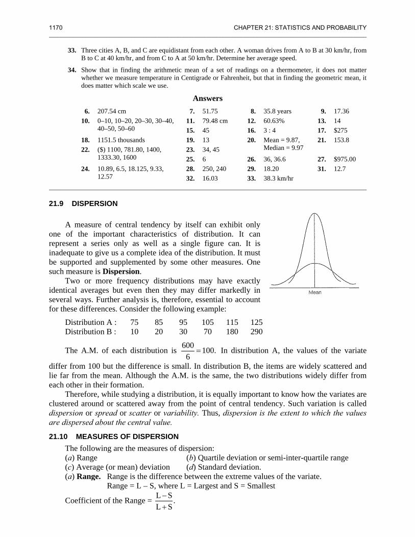
A mone of representinadequabe supposuch mea
Twoidentical several wfor these
DistDist
The
differ frolie far froeach othe
Theclustereddispersioare dispe
21.10 MThe(a) R(c) A(a) R
Coe
______________
Three cities AB to C at 40 k
Show that inwhether we mdoes matter w
6. 207.54 10. 0–10, 1
40–50, 18. 1151.5 22. ($) 110
1333.30 24. 10.89,
12.57 ______________
ISPERSION
measure of cthe importat a series oate to give usorted and suasure is Dispo or more
averages bways. Furthe
differences.
tribution A :tribution B :
A.M. of ea
om 100 but tom the meaer in their forefore, while
d around or on or spreadersed about t
MEASURES following aRange Average (or Range. Ran
Ran
efficient of th
_____________
A, B, and C arekm/hr, and from
n finding the ameasure tempewhich scale we
cm 10–20, 20–30, 50–60
thousands 00, 781.80, 1400, 1600
6.5, 18.125, 9.
_____________
N
central tendeant characteonly as wels a completeupplementedpersion. frequency dut even the
er analysis is. Consider th
75 10 2
ach distribut
the differencn. Althoughrmation. e studying a scattered aw
d or scatter othe central v
S OF DISPEare the measu
mean) deviange is the dinge = L – S,
he Range =
______________
e equidistant frm C to A at 50
arithmetic meaerature in Cente use.
A7.
30–40, 11.15.19.
00, 23.25.
33, 28.32.
______________
ency by itseeristics of l as a sing
e idea of the d by some o
distributionsn they mays, therefore, he following
85 9520 30
tion is 6006
ce is small. h the A.M. is
distributionway from theor variabilityvalue.
RSION ures of dispe
(b)ation (d)ifference bet, where L = LL S .L S
−+
______________
rom each other0 km/hr. Determ
an of a set of igrade or Fahr
Answers . 51.75 . 79.48 cm . 45 . 13 . 34, 45 . 6 . 250, 240 . 16.03 ______________
elf can exhidistribution.
gle figure cadistribution
other measur
may have y differ mark
essential to g example:
105 1170 18
100.= In d
In distributis the same,
n, it is equalle point of cey. Thus, disp
ersion: ) Quartile de) Standard dtween the exLargest and
CHAPTER 21_____________
r. A woman drimine her avera
f readings on arenheit, but tha
8. 35.12. 60.16. 3 : 20. Me
Me 26. 36,29. 18.33. 38.
_____________
ibit only . It can an. It is
n. It must res. One
exactly kedly in account
15 125 80 290
distribution
on B, the itethe two dist
y important entral tendenpersion is th
eviation or sedeviation. xtreme value
S = Smalles
: STATISTICS ______________
ives from A toge speed.
a thermometerat in finding th
8 years 63% 4
ean = 9.87, edian = 9.97
, 36.6 20 3 km/hr
______________
A, the valu
ems are widtributions w
to know howncy. Such vhe extent to
emi-inter-qu
s of the variast
AND PROBAB______________
B at 30 km/hr
r, it does not me geometric m
9. 17.3613. 14 17. $27521. 153.8
27. $975.31. 12.7
______________
ues of the va
dely scatteredwidely differ
w the variatevariation is cwhich the v
uartile range
ate.
BILITY ______
r, from
matter mean, it
00
______
ariate
d and from
es are called values
21.10 MEASURES OF DISPERSION 1171 ________________________________________________________________________________________________________
It is easily understood and computed. But it suffers from the drawback that it depends exclusively on the two extreme values. It is not a reliable measure of dispersion.
(b) Quartile Deviation. The difference between the upper and lower quartiles, i.e., Q3 – Q1 is known as the inter-quartile range and half of it, i.e., 1
2 (Q3 – Q1), is called the semi- inter-quartile range or the quartile deviation.
Quartile Deviation = 3 11 (Q Q ).2
−
It is definitely a better measure of dispersion than range as it makes use of 50% of the data. But since it ignores the other 50% of the data, it is also not a reliable measure of dispersion.
Coefficient of the Quartile Deviation = 3 1
3 1
Q Q .Q Q
−+
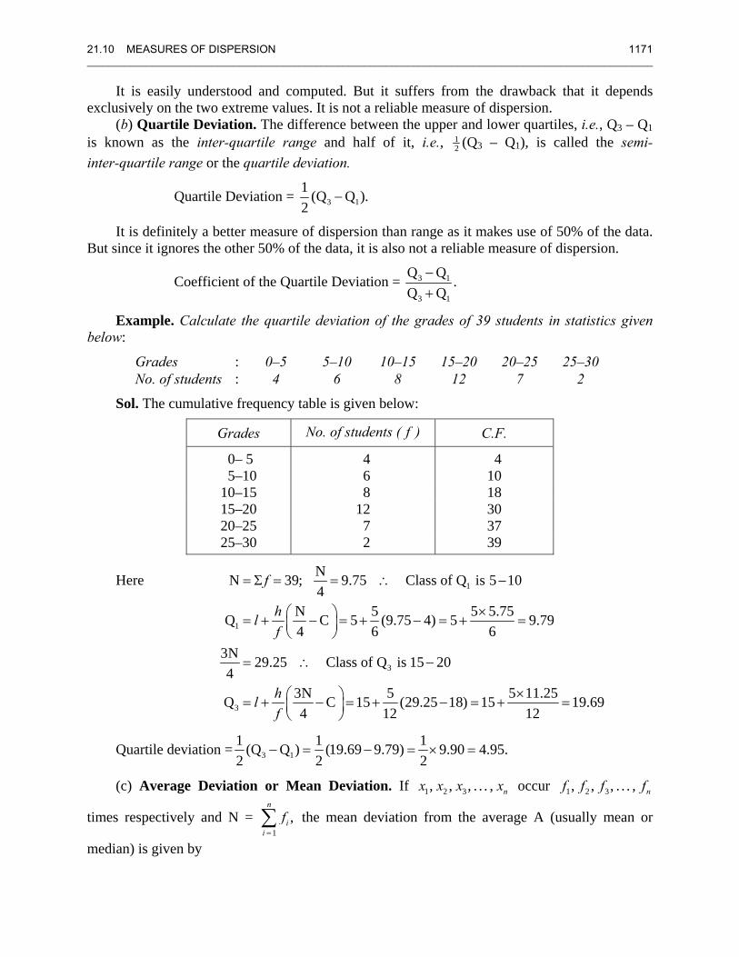
Example. Calculate the quartile deviation of the grades of 39 students in statistics given below:
Grades : 0–5 5–10 10–15 15–20 20–25 25–30 No. of students : 4 6 8 12 7 2
Sol. The cumulative frequency table is given below:
Grades No. of students ( f ) C.F.
0– 5 4 4 5–10 6 10 10–15 8 18 15–20 12 30 20–25 7 37 25–30 2 39
Here 1
1
3
3
NN 39; 9.75 Class of Q is 5 104
N 5 5 5.75Q C 5 (9.75 4) 5 9.794 6 6
3N 29.25 Class of Q is 15 204
3N 5 5 11.25Q C 15 (29.25 18) 15 19.694 12 12
f
hlf
hlf
= Σ = = ∴ −
×⎛ ⎞= + − = + − = + =⎜ ⎟⎝ ⎠
= ∴ −
×⎛ ⎞= + − = + − = + =⎜ ⎟⎝ ⎠
Quartile deviation = 3 11 1 1(Q Q ) (19.69 9.79) 9.90 4.95.2 2 2
− = − = × =
(c) Average Deviation or Mean Deviation. If 1 2 3, , , . . . , nx x x x occur 1 2 3, , , . . . , nf f f f
times respectively and N = 1
,n
ii
f=∑ the mean deviation from the average A (usually mean or
median) is given by
1172 CHAPTER 21: STATISTICS AND PROBABILITY ________________________________________________________________________________________________________
1
1 A ,N
n
i ii
Mean deviation f x=
= −∑
where Aix − represents the modulus or the absolute value of the deviation (xi – A). Since the mean deviation is based on all the values of the variate, it is a better measure of
dispersion than range or quartile deviation. But some artificiality is created due to ignoring the signs of the deviations (xi – A). This renders it useless for further mathematical treatment.
Mean DeviationCoefficient of Mean Deviation .Average from which it is calculated
=
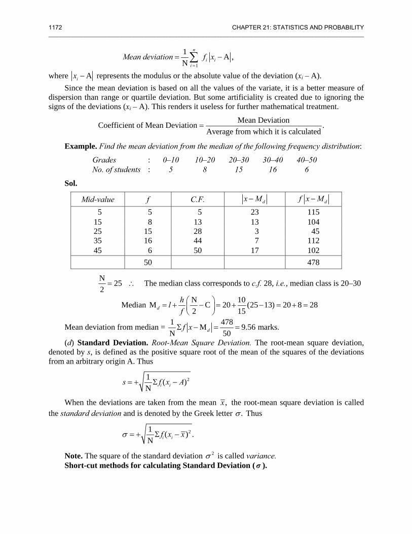
Example. Find the mean deviation from the median of the following frequency distribution:
Grades : 0–10 10–20 20–30 30–40 40–50 No. of students : 5 8 15 16 6
Sol.
Mid-value f C.F. dx M− df x M−
5 5 5 23 115 15 8 13 13 104 25 15 28 3 45 35 16 44 7 112 45 6 50 17 102 50 478
N 252
= ∴ The median class corresponds to c.f. 28, i.e., median class is 20–30
Median N 10M C 20 (25 13) 20 8 282 15d
hlf
⎛ ⎞= + − = + − = + =⎜ ⎟⎝ ⎠
Mean deviation from median = 1 478M 9.56 marks.N 50df xΣ − = =
(d) Standard Deviation. Root-Mean Square Deviation. The root-mean square deviation, denoted by s, is defined as the positive square root of the mean of the squares of the deviations from an arbitrary origin A. Thus
21 ( )N i is f x A= + Σ −
When the deviations are taken from the mean ,x the root-mean square deviation is called the standard deviation and is denoted by the Greek letter .σ Thus
21 ( ) .N i if x xσ = + Σ −
Note. The square of the standard deviation 2σ is called variance. Short-cut methods for calculating Standard Deviation (σ ).
21.10 MEASURES OF DISPERSION 1173 ________________________________________________________________________________________________________
(i) Direct Method
⇒
2
2 2 2 2 2
1 ( )N
1 1 1 1( 2 ) 2N N N N
i i
i i i i i i i i
f x x
f x x x x f x x f x x f
σ
σ
= Σ −
= Σ − + = Σ − ⋅ Σ + ⋅ Σ
(taking the constants 2,x x outside the summation sign)
⇒
2 2 2 2
22 2 2
1 1 12 NN N N
1 1 1 .N N N
i i i i
i i i i i i
f x x x x f x x
f x x f x f xσ
= Σ − ⋅ + ⋅ ⋅ = Σ −
⎛ ⎞= Σ − = Σ − Σ⎜ ⎟⎝ ⎠
(ii) Change of Origin Let the origin be shifted to an arbitrary point a. Let d = x – a denote the deviation of variate
x from the new origin
∴
2 21 1( ) ( )N Nx d
d x a d x ad d x x
f x x f d dσ σ
= − ⇒ = −
− = −
= Σ − = Σ − =
∴ The S.D. remains unchanged by shift of origin.
2
21 1 .N Nx d fd fdσ σ ⎛ ⎞= Σ − Σ⎜ ⎟
⎝ ⎠
Note. In the case of series of individual observations, if the mean is a whole number, take a = .x In the case of discrete series, when the values of x are not equidistant, take a somewhere in the middle of the x-series.
(iii) Shift of Origin and Change of Scale (Step Deviation Method)
Let the origin be shifted to an arbitrary point a. Let the new scale be 1h
times the original
Let
2 2 2 2
then ( )
1 1 1( ) ( ) ( )N N Nx u
x au hu x a hu x a h u u x xh
f x x fh u u h f u u hσ σ
−= = − ⇒ = − ∴ − = −
= Σ − = Σ − = Σ − =
which is independent of a but not h. Hence the S.D. is independent of the change of the origin but not of the change of scale.
2
21 1N Nx uh h fu fuσ σ ⎛ ⎞= = Σ − Σ⎜ ⎟
⎝ ⎠
Note. In the case of discrete series, when the values of x are equidistant at intervals of h or in the case of continuous series having equal class intervals of width h, use the Step Deviation Method.
scale.
1174 CHAPTER 21: STATISTICS AND PROBABILITY ________________________________________________________________________________________________________
Relation between σ and s By definition, we have
Hence
2 2 2
2
2 2
2 22 2
2 2
2
1 1( ) ( )N N1 ( ) whereN1 [( ) 2 ( )]N1 2 2( ) ( ) N (0)N N N N N
[ ( ) algebraic sum of the deviations from mean 0]
i i i i
i i
i i i
i i i i i
i i
s f x a f x x x a
f x x d d x a
f x x d d x x
d d d df x x f f x x
f x x
ds
σ
σ
σ
= Σ − = Σ − + −
= Σ − + = −
= Σ − + + −
= Σ − + Σ + Σ − = + ⋅ +
Σ − = =
= +
=
∵
2 2 2 2 20d d s σ+ ≥ ∴ ≥∵ Clearly s2 is least when d = 0, i.e., x = a ∴ Mean square deviation (s2) and consequently the root-mean square deviation (s) is least
when the deviations are measured from the mean. Hence standard deviation is the least possible root-mean square deviation.
21.11 RELATIONS BETWEEN MEASURES OF DISPERSION
Mean Deviation = 45
(standard deviation) = 45
σ
Semi-interquartile range = 23
(standard deviation) = 2 .3
σ
21.12 COEFFICIENT OF DISPERSION Whenever we want to compare the variability of two series that differ widely in their
averages or which are measured in different units, we calculate the coefficients of dispersion, which being ratios are numbers independent of the units of measurement. The coefficients of dispersion (C.D.) based on different measures of dispersion are as follows:
(a) C.D. based on range: max min
max min
x xx x
−=
+
(b) Based on quartile deviation: 3 1
3 1
Q QC.D.Q Q
−=
+
(c) Based on mean deviation: mean deviationC.D.average from which it is calculated
=
(d) Based on standard deviation: S.D.C.D.Mean x
σ= =
Coefficient of variation. It is the percentage variation in the mean, standard deviation being considered as the total variation in the mean.
C.V. 100.xσ
= ×
21.12 COEFFICIENT OF DISPERSION 1175 ________________________________________________________________________________________________________
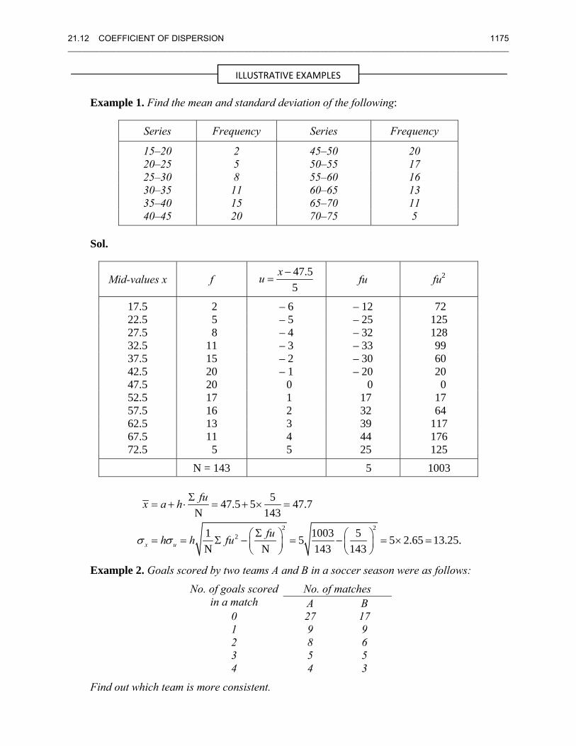
Example 1. Find the mean and standard deviation of the following:
Series Frequency Series Frequency
15–20 2 45–50 20 20–25 5 50–55 17 25–30 8 55–60 16 30–35 11 60–65 13 35–40 15 65–70 11 40–45 20 70–75 5
Sol.
Mid-values x f 47.55
xu −= fu fu2
17.5 2 – 6 – 12 72 22.5 5 – 5 – 25 125 27.5 8 – 4 – 32 128 32.5 11 – 3 – 33 99 37.5 15 – 2 – 30 60 42.5 20 – 1 – 20 20 47.5 20 0 0 0 52.5 17 1 17 17 57.5 16 2 32 64 62.5 13 3 39 117 67.5 11 4 44 176 72.5 5 5 25 125
N = 143 5 1003
2 22
547.5 5 47.7N 143
1 1003 55 5 2.65 13.25.N N 143 143x u
fux a h
fuh h fuσ σ
Σ= + ⋅ = + × =
Σ⎛ ⎞ ⎛ ⎞= = Σ − = − = × =⎜ ⎟ ⎜ ⎟⎝ ⎠ ⎝ ⎠
Example 2. Goals scored by two teams A and B in a soccer season were as follows:
No. of goals scoredin a match
No. of matches A B
0 27 17 1 9 9 2 8 6 3 5 5 4 4 3
Find out which team is more consistent.
ILLUSTRATIVE EXAMPLES
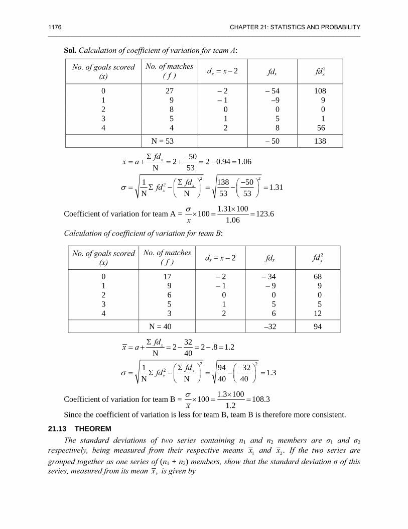
1176 CHAPTER 21: STATISTICS AND PROBABILITY ________________________________________________________________________________________________________
Sol. Calculation of coefficient of variation for team A:
No. of goals scored (x)
No. of matches ( f ) 2xd x= − fdx 2
xfd
0 27 – 2 – 54 108 1 9 – 1 –9 9 2 8 0 0 0 3 5 1 5 1 4 4 2 8 56
N = 53 – 50 138
2 22
502 2 0.94 1.06N 53
1 138 50 1.31N N 53 53
x
xx
fdx a
fdfdσ
Σ −= + = + = − =
Σ −⎛ ⎞ ⎛ ⎞= Σ − = − =⎜ ⎟⎜ ⎟⎝ ⎠⎝ ⎠
Coefficient of variation for team A = 1.31 100100 123.61.06x
σ ×× = =
Calculation of coefficient of variation for team B:
No. of goals scored (x)
No. of matches ( f ) dx = x – 2 fdx 2
xfd
0 17 – 2 – 34 68 1 9 – 1 – 9 9 2 6 0 0 0 3 5 1 5 5 4 3 2 6 12
N = 40 –32 94
2 22
322 2 .8 1.2N 40
1 94 32 1.3N N 40 40
x
xx
fdx a
fdfdσ
Σ= + = − = − =
Σ −⎛ ⎞ ⎛ ⎞= Σ − = − =⎜ ⎟⎜ ⎟⎝ ⎠⎝ ⎠
Coefficient of variation for team B = 1.3 100100 108.31.2x
σ ×× = =
Since the coefficient of variation is less for team B, team B is therefore more consistent.
21.13 THEOREM The standard deviations of two series containing n1 and n2 members are σ1 and σ2
respectively, being measured from their respective means 1x and 2.x If the two series are grouped together as one series of (n1 + n2) members, show that the standard deviation σ of this series, measured from its mean ,x is given by
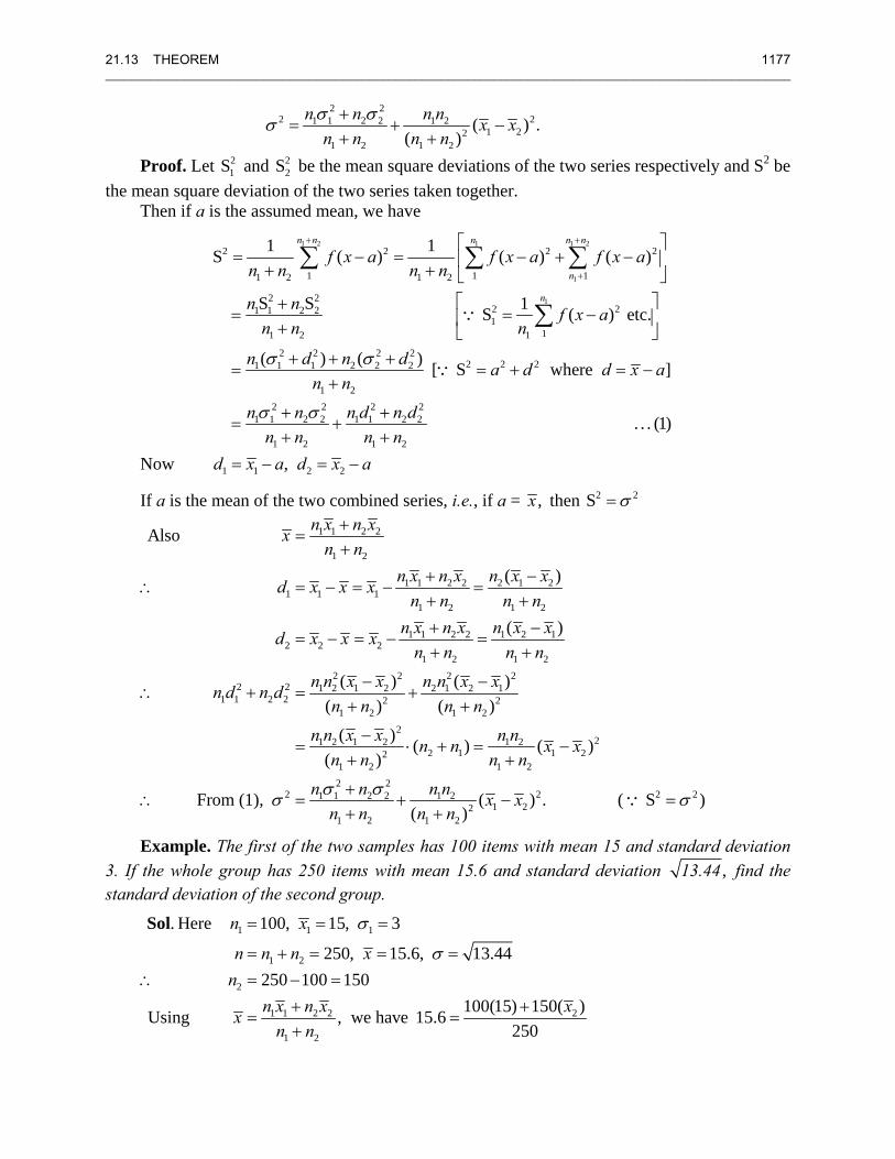
21.13 THEOREM 1177 ________________________________________________________________________________________________________
2 2
2 21 1 2 2 1 21 22
1 2 1 2
( ) .( )
n n n n x xn n n n
σ σσ += + −
+ +
Proof. Let 21S and 2
2S be the mean square deviations of the two series respectively and S2 be the mean square deviation of the two series taken together.
Then if a is the assumed mean, we have
Now
1 2 1 1 2
1
1
2 2 2 2
1 1 11 2 1 2
2 22 21 1 2 21
11 2 1
2 2 2 22 2 21 1 1 2 2 2
1 22 2 2 2
1 1 2 2 1 1 2 2
1 2 1 2
1 1S ( ) ( ) ( )
S S 1S ( ) etc.
( ) ( ) [ S where ]
. . . (
n n n n n
n
n
f x a f x a f x an n n n
n n f x an n n
n d n d a d d x an n
n n n d n dn n n n
σ σ
σ σ
+ +
+
⎡ ⎤= − = − + −⎢ ⎥+ + ⎣ ⎦
⎡ ⎤+= = −⎢ ⎥+ ⎣ ⎦
+ + += = + = −
+
+ += +
+ +
∑ ∑ ∑
∑∵
∵
1 1 2 2
1)
,d x a d x a= − = −
If a is the mean of the two combined series, i.e., if a = ,x then 2 2S σ= 1 1 2 2
1 2
1 1 2 2 2 1 21 1 1
1 2 1 2
1 1 2 2 1 2 12 2 2
1 2 1 22 2 2 2
2 2 1 2 1 2 2 1 2 11 1 2 2 2 2
1 2 1 22
1 2 1 2 1 22 1 12
1 2 1 2
Also
( )
( )
( ) ( )( ) ( )
( ) ( ) (( )
n x n xxn n
n x n x n x xd x x xn n n n
n x n x n x xd x x xn n n n
n n x x n n x xn d n dn n n n
n n x x n nn n xn n n n
+=
++ −
∴ = − = − =+ ++ −
= − = − =+ +
− −∴ + = +
+ +
−= ⋅ + = −
+ +2
2
2 22 2 2 21 1 2 2 1 2
1 221 2 1 2
)
From (1), ( ) . ( S )( )
x
n n n n x xn n n n
σ σσ σ+∴ = + − =
+ +∵
Example. The first of the two samples has 100 items with mean 15 and standard deviation 3. If the whole group has 250 items with mean 15.6 and standard deviation ,13.44 find the standard deviation of the second group.
1 1 1
1 2
2
1 1 2 2 2
1 2
. Here 100, 15, 3
250, 15.6, 13.44250 100 150
100(15) 150( )Using , we have 15.6250
n x
n n n xn
n x n x xxn n
σ
σ
= = =
= + = = =∴ = − =
+ += =
+
Sol
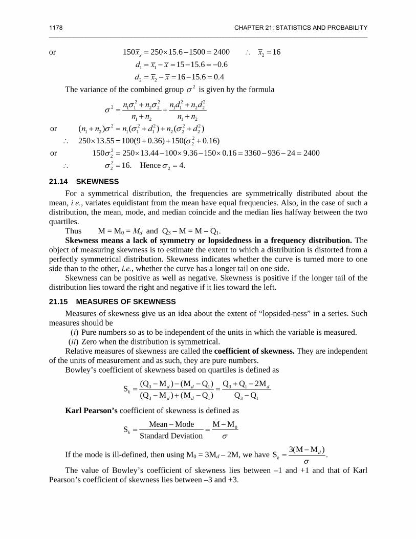
1178 CHAPTER 21: STATISTICS AND PROBABILITY ________________________________________________________________________________________________________
or 2
1 1
2 2
150 250 15.6 1500 2400 1615 15.6 0.616 15.6 0.4
xx xd x xd x x
= × − = ∴ == − = − = −= − = − =
The variance of the combined group 2σ is given by the formula 2 2 2 2
2 1 1 2 2 1 1 2 2
1 2 1 22 2 2 2 2
1 2 1 1 1 2 2 222
2222 2
or ( ) ( ) ( )250 13.55 100(9 0.36) 150( 0.16)
or 150 250 13.44 100 9.36 150 0.16 3360 936 24 240016. Hence 4.
n n n d n dn n n n
n n n d n d
σ σσ
σ σ σσ
σσ σ
+ += +
+ ++ = + + +
∴ × = + + += × − × − × = − − =
∴ = =
21.14 SKEWNESS For a symmetrical distribution, the frequencies are symmetrically distributed about the
mean, i.e., variates equidistant from the mean have equal frequencies. Also, in the case of such a distribution, the mean, mode, and median coincide and the median lies halfway between the two quartiles.
Thus M = M0 = Md and Q3 – M = M – Q1. Skewness means a lack of symmetry or lopsidedness in a frequency distribution. The
object of measuring skewness is to estimate the extent to which a distribution is distorted from a perfectly symmetrical distribution. Skewness indicates whether the curve is turned more to one side than to the other, i.e., whether the curve has a longer tail on one side.
Skewness can be positive as well as negative. Skewness is positive if the longer tail of the distribution lies toward the right and negative if it lies toward the left.
21.15 MEASURES OF SKEWNESS Measures of skewness give us an idea about the extent of “lopsided-ness” in a series. Such
measures should be (i) Pure numbers so as to be independent of the units in which the variable is measured. (ii) Zero when the distribution is symmetrical. Relative measures of skewness are called the coefficient of skewness. They are independent
of the units of measurement and as such, they are pure numbers. Bowley’s coefficient of skewness based on quartiles is defined as
3 1 3 1
3 1 3 1
(Q M ) (M Q ) Q Q 2MS(Q M ) (M Q ) Q Q
d d dk
d d
− − − + −= =
− + − −
Karl Pearson’s coefficient of skewness is defined as
0M MMean ModeSStandard Deviationk σ
−−= =
If the mode is ill-defined, then using M0 = 3Md – 2M, we have 3(M M )S .dk σ
−=
The value of Bowley’s coefficient of skewness lies between –1 and +1 and that of Karl Pearson’s coefficient of skewness lies between –3 and +3.
21.16 MOMENTS 1179 ________________________________________________________________________________________________________
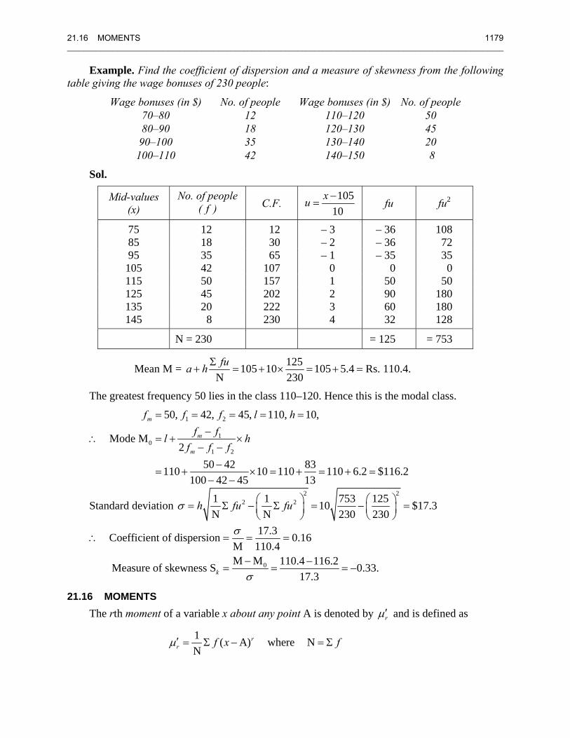
Example. Find the coefficient of dispersion and a measure of skewness from the following table giving the wage bonuses of 230 people:
Wage bonuses (in $) No. of people Wage bonuses (in $) No. of people70–80 12 110–120 50 80–90 18 120–130 45 90–100 35 130–140 20 100–110 42 140–150 8
Sol.
Mid-values (x)
No. of people ( f ) C.F.
10510
xu −= fu fu2
75 12 12 – 3 – 36 108 85 18 30 – 2 – 36 72 95 35 65 – 1 – 35 35 105 42 107 0 0 0 115 50 157 1 50 50 125 45 202 2 90 180 135 20 222 3 60 180 145 8 230 4 32 128
N = 230 = 125 = 753
Mean M = 125105 10 105 5.4 Rs. 110.4.N 230fua h Σ
+ = + × = + =
The greatest frequency 50 lies in the class 110–120. Hence this is the modal class.
1 2
10
1 2
50, 42, 45, 110, 10,
Mode M2
50 42 83110 10 110 110 6.2 $116.2100 42 45 13
m
m
m
f f f l hf fl h
f f f
= = = = =−
∴ = + ×− −
−= + × = + = + =
− −
Standard deviation 2 2
2 21 1 753 12510 $17.3N N 230 230
h fu fuσ ⎛ ⎞ ⎛ ⎞= Σ − Σ = − =⎜ ⎟ ⎜ ⎟⎝ ⎠ ⎝ ⎠
0
17.3Coefficient of dispersion 0.16M 110.4M M 110.4 116.2Measure of skewness S 0.33.
17.3k
σ
σ
∴ = = =
− −= = = −
21.16 MOMENTS The rth moment of a variable x about any point A is denoted by rμ′ and is defined as
1 ( A) where NN
rr f x fμ′ = Σ − = Σ
1180 CHAPTER 21: STATISTICS AND PROBABILITY ________________________________________________________________________________________________________
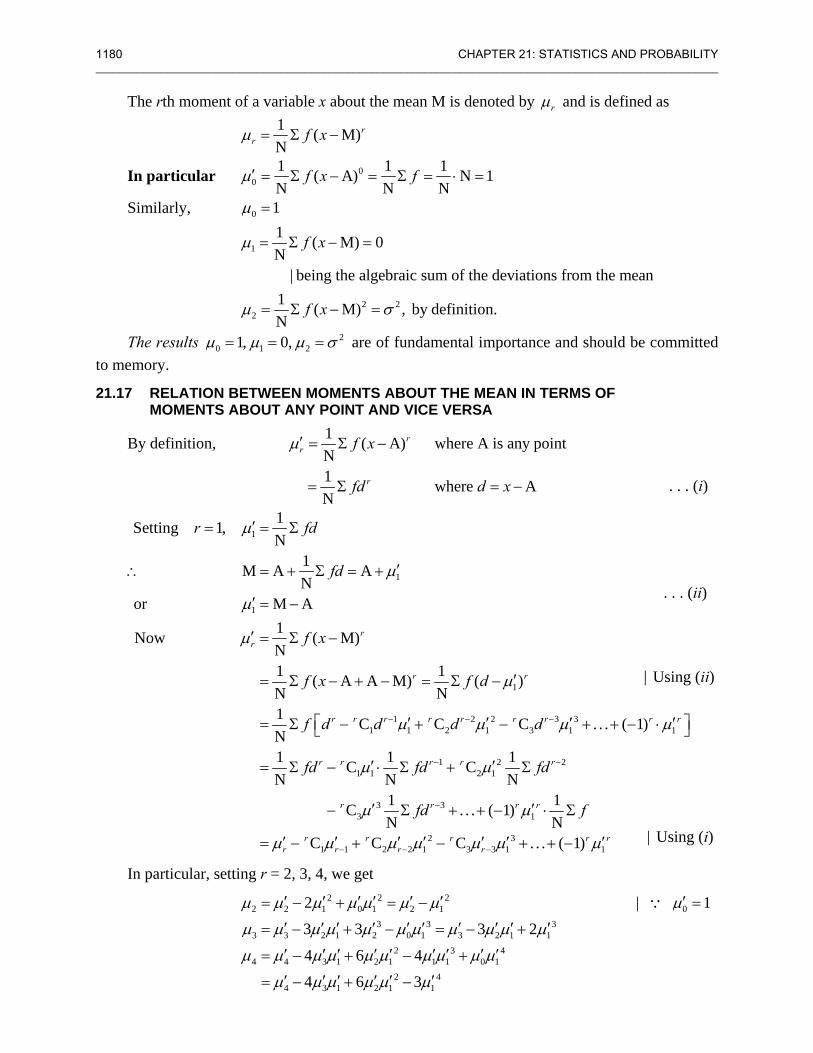
The rth moment of a variable x about the mean M is denoted by rμ and is defined as
1 ( M)N
rr f xμ = Σ −
In particular 00
1 1 1( A) N 1N N N
f x fμ′ = Σ − = Σ = ⋅ =
Similarly, 0
1
2 22
11 ( M) 0N
| being the algebraic sum of the deviations from the mean1 ( M) , by definition.N
f x
f x
μ
μ
μ σ
=
= Σ − =
= Σ − =
The results 20 1 21, 0,μ μ μ σ= = = are of fundamental importance and should be committed
to memory.
21.17 RELATION BETWEEN MOMENTS ABOUT THE MEAN IN TERMS OF MOMENTS ABOUT ANY POINT AND VICE VERSA
By definition, 1 ( A) where A is any pointN1 where AN
rr
r
f x
fd d x
μ′ = Σ −
= Σ = −
1
1
1
1
1 2 2 3 31 1 2 1 3 1 1
1 2 21 1 2 1
33
1Setting 1,N
1M A AN
or M A1Now ( M)N1 1( A A M) ( )N N1 C C C . . . ( 1)N1 1 1C CN N N
1CN
rr
r r
r r r r r r r r r
r r r r r
r
r fd
fd
f x
f x f d
f d d d d
fd fd fd
μ
μ
μ
μ
μ
μ μ μ μ
μ μ
μ
− − −
− −
′= = Σ
′∴ = + Σ = +
′ = −
′ = Σ −
′= Σ − + − = Σ −
′ ′ ′ ′⎡ ⎤= Σ − + − + + − ⋅⎣ ⎦
′ ′= Σ − ⋅ Σ + Σ
′− Σ 31
2 31 1 2 2 1 3 3 1 1
1. . . ( 1)N
C C C . . . ( 1)
r r r
r r r r rr r r r
fd fμ
μ μ μ μ μ μ μ
−
− − −
′+ + − ⋅ Σ
′ ′ ′ ′ ′ ′ ′= − + − + + − In particular, setting r = 2, 3, 4, we get
2 2 22 2 1 0 1 2 1
3 3 33 3 2 1 2 0 1 3 2 1 1
2 3 44 4 3 1 2 1 1 1 0 1
2 44 3 1 2 1 1
2
3 3 3 2
4 6 4
4 6 3
μ μ μ μ μ μ μ
μ μ μ μ μ μ μ μ μ μ μ
μ μ μ μ μ μ μ μ μ μ
μ μ μ μ μ μ
′ ′ ′ ′ ′ ′= − + = −
′ ′ ′ ′ ′ ′ ′ ′ ′ ′= − + − = − +
′ ′ ′ ′ ′ ′ ′ ′ ′= − + − +
′ ′ ′ ′ ′ ′= − + −
0| 1μ′ =∵
. . . (i)
| Using (ii)
| Using (i)
. . . (ii)
21.19 SHEPPARD’S CORRECTIONS FOR MOMENTS 1181 ________________________________________________________________________________________________________
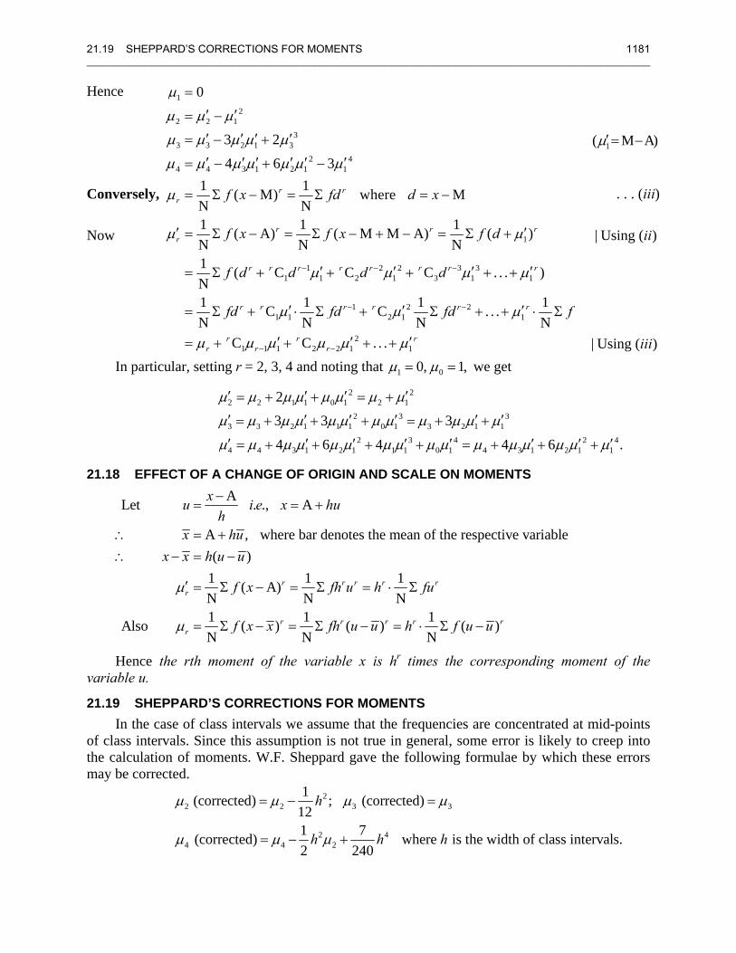
Hence 12
2 2 13
3 3 2 1 32 4
4 4 3 1 2 1 1
1
1 2 2 3 31 1 2 1 3 1 1
1
0
3 2
4 6 31 1( M) where MN N1 1 1( A) ( M M A) ( )N N N1 ( C C C . . . )N1 CN
r rr
r r rr
r r r r r r r r
r r
f x fd d x
f x f x f d
f d d d d
fd
μ
μ μ μ
μ μ μ μ μ
μ μ μ μ μ μ μ
μ
μ μ
μ μ μ μ− − −
=
′ ′= −
′ ′ ′ ′= − +
′ ′ ′ ′ ′ ′= − + −
= Σ − = Σ = −
′ ′= Σ − = Σ − + − = Σ +
′ ′ ′ ′= Σ + + + + +
= Σ + 1 2 21 2 1 1
21 1 1 2 2 1 1
1 1 1C . . .N N N
C C . . .
r r r r
r r rr r r
fd fd fμ μ μ
μ μ μ μ μ μ
− −
− −
′ ′ ′⋅ Σ + Σ + + ⋅ Σ
′ ′ ′= + + + +
1( M A)μ′= −
Conversely, . . . (iii)
Now | Using ( )ii
| Using ( )iiiIn particular, setting r = 2, 3, 4 and noting that 1 00, 1,μ μ= = we get
2 22 2 1 1 0 1 2 1
2 3 33 3 2 1 1 1 0 1 3 2 1 1
2 3 4 2 44 4 3 1 2 1 1 1 0 1 4 3 1 2 1 1
2
3 3 3
4 6 4 4 6 .
μ μ μ μ μ μ μ μ
μ μ μ μ μ μ μ μ μ μ μ μ
μ μ μ μ μ μ μ μ μ μ μ μ μ μ μ μ
′ ′ ′ ′= + + = +
′ ′ ′ ′ ′ ′= + + + = + +
′ ′ ′ ′ ′ ′ ′ ′= + + + + = + + +
21.18 EFFECT OF A CHANGE OF ORIGIN AND SCALE ON MOMENTS ALet . ., A
A , where bar denotes the mean of the respective variable( )
1 1 1( A)N N N1 1 1Also ( ) ( ) ( )N N N
r r r r rr
r r r r rr
xu i e x huh
x hux x h u u
f x fh u h fu
f x x fh u u h f u u
μ
μ
−= = +
∴ = +∴ − = −
′ = Σ − = Σ = ⋅ Σ
= Σ − = Σ − = ⋅ Σ −
Hence the rth moment of the variable x is hr times the corresponding moment of the variable u.
21.19 SHEPPARD’S CORRECTIONS FOR MOMENTS In the case of class intervals we assume that the frequencies are concentrated at mid-points
of class intervals. Since this assumption is not true in general, some error is likely to creep into the calculation of moments. W.F. Sheppard gave the following formulae by which these errors may be corrected.
22 2 3 3
2 44 4 2
1(corrected) ; (corrected)121 7 (corrected) where is the width of class intervals.2 240
h
h h h
μ μ μ μ
μ μ μ
= − =
= − +
1182 __________
21.20 CTo
following
21.21 PKarl
about the
Thenumbers.
Base
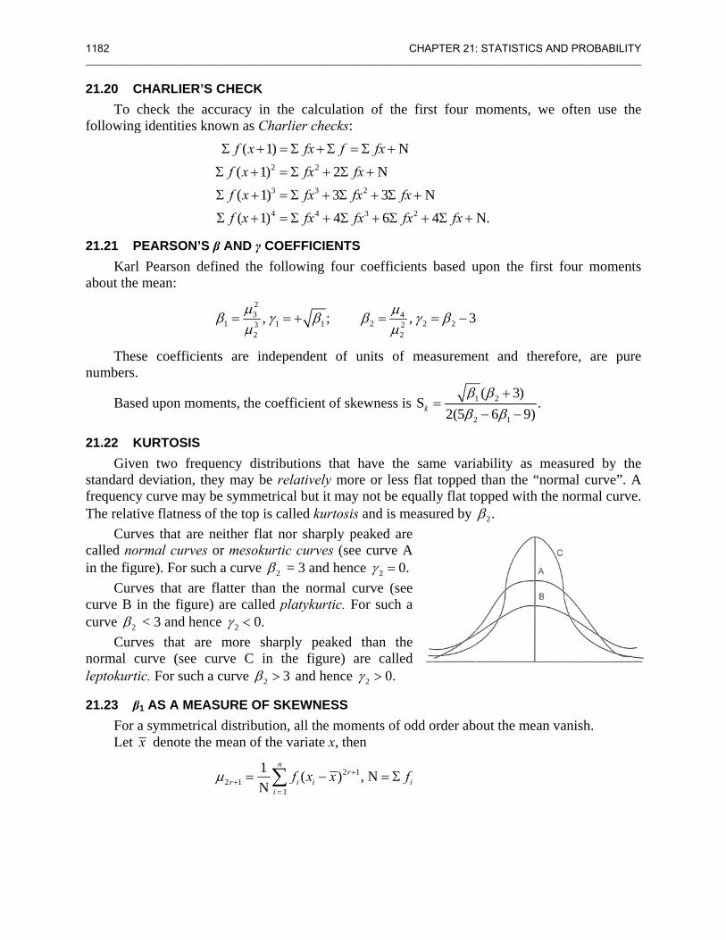
21.22 KGive
standard frequencyThe relat
Curvcalled noin the fig
Curvcurve B curve 2β
Curvnormal cleptokurt
21.23 βFor Let
______________
CHARLIER’check the ag identities k
PEARSON’Sl Pearson de mean:
se coefficie.
ed upon mom
KURTOSIS en two freqdeviation, ty curve maytive flatness ves that are
ormal curvesgure). For sucves that arein the figure < 3 and henves that arcurve (see tic. For such
β1 AS A MEAa symmetricx denote th
_____________
S CHECK accuracy in known as Ch
2
3
4
( 1( 1)( 1)( 1)
f xf xf xf x
Σ +
Σ +
Σ +
Σ +
S β AND γ Cefined the f
23
1 32
,μβ γμ
=
ents are ind
ments, the co
quency distrthey may bey be symmetof the top isneither flat
s or mesokuch a curve β
e flatter thane) are callednce 2 0.γ < re more shcurve C in
h a curve 2β
ASURE OF cal distributihe mean of th
2 11Nrμ + =
______________
the calculaharlier check
2 2
3 3
4 4
)234
fx ffxfxfx
= Σ + Σ
= Σ +
= Σ + Σ
= Σ +
COEFFICIENfollowing fo
1 1 ;γ β= +
dependent o
oefficient of
ributions the relatively mtrical but it ms called kurtot nor sharplyrtic curves (
2β = 3 and hn the normad platykurtic
harply peaken the figure
3> and hen
SKEWNESion, all the mhe variate x,
1
( )n
i ii
f x x=
−∑
______________
ation of the ks:
2
3
N2 N
34 6
f fxfxfx fxfx fx
= Σ +
Σ +
Σ + Σ
Σ + Σ
NTS our coefficie
42 2
2
μβμ
=
of units of
f skewness is
hat have themore or lessmay not be eosis and is my peaked are(see curve A
hence 2 0.γ =al curve (seec. For such a
ed than thee) are callednce 2 0.γ >
S moments of o
then
2 1) , Nr f+ = Σ
CHAPTER 21_____________
first four m
2
N
N4
fxfx fx
+
+ Σ +
ents based u
2 2, 3γ β= −
measureme
s 2
S2(5k
ββ
=
e same varis flat toppedqually flat to
measured by e
A . e a
e d
odd order ab
if
: STATISTICS ______________
moments, w
N.
upon the fir
ent and the
1 2
2 1
( 3).
6 9)β β
β+
− −
iability as md than the “nopped with t
2.β
bout the mean
AND PROBAB______________
we often use
rst four mom
erefore, are
measured bynormal curvethe normal c
n vanish.
BILITY ______
e the
ments
pure
y the e”. A
curve.
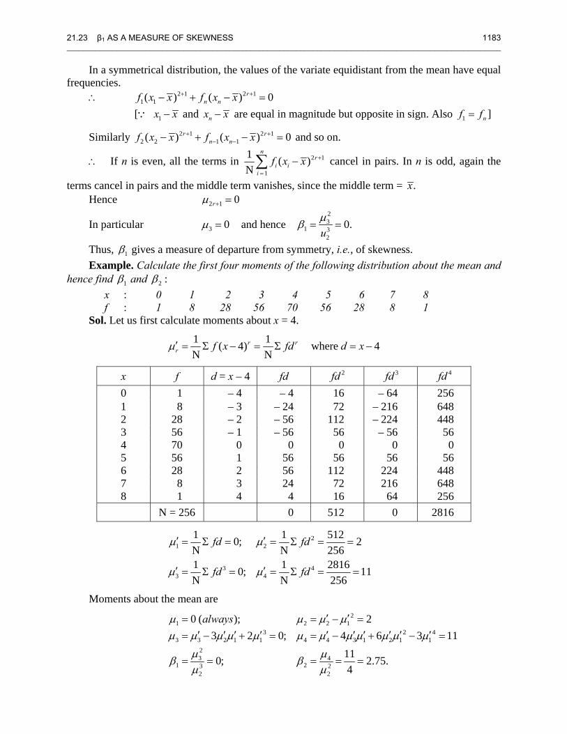
21.23 β1 AS A MEASURE OF SKEWNESS 1183 ________________________________________________________________________________________________________
In a symmetrical distribution, the values of the variate equidistant from the mean have equal frequencies.
∴ 2 1 2 11 1( ) ( ) 0r
n nf x x f x x+ +− + − = 1[ x x−∵ and nx x− are equal in magnitude but opposite in sign. Also 1 ]nf f=
Similarly 2 1 2 12 2 1 1( ) ( ) 0r r
n nf x x f x x+ +− −− + − = and so on.
∴ If n is even, all the terms in 2 1
1
1 ( )N
nr
i ii
f x x +
=
−∑ cancel in pairs. In n is odd, again the
terms cancel in pairs and the middle term vanishes, since the middle term = .x Hence 2 1 0rμ + =
In particular 23
3 1 32
0 and hence 0.uμμ β= = =
Thus, 1β gives a measure of departure from symmetry, i.e., of skewness. Example. Calculate the first four moments of the following distribution about the mean and
hence find 1β and 2 :β x : 0 1 2 3 4 5 6 7 8
f : 1 8 28 56 70 56 28 8 1 Sol. Let us first calculate moments about x = 4.
1 1( 4) where 4N N
r rr f x fd d xμ′ = Σ − = Σ = −
x f d = x – 4 fd 2fd 3fd 4fd 0 1 – 4 – 4 16 – 64 256 1 8 – 3 – 24 72 – 216 648 2 28 – 2 – 56 112 – 224 448 3 56 – 1 – 56 56 – 56 56 4 70 0 0 0 0 0 5 56 1 56 56 56 56 6 28 2 56 112 224 448 7 8 3 24 72 216 648 8 1 4 4 16 64 256 N = 256 0 512 0 2816
21 2
3 43 4
1 1 5120; 2N N 2561 1 28160; 11N N 256
fd fd
fd fd
μ μ
μ μ
′ ′= Σ = = Σ = =
′ ′= Σ = = Σ = =
Moments about the mean are
21 2 2 1
3 2 43 3 2 1 1 4 4 3 1 2 1 1
23 4
1 23 22 2
0 ( ); 23 2 0; 4 6 3 11
110; 2.75.4
alwaysμ μ μ μμ μ μ μ μ μ μ μ μ μ μ μ
μ μβ βμ μ
′ ′= = − =′ ′ ′ ′ ′ ′ ′ ′ ′ ′= − + = = − + − =
= = = = =
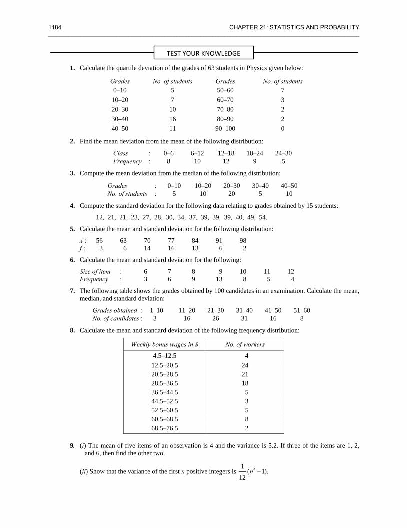
1184 CHAPTER 21: STATISTICS AND PROBABILITY ________________________________________________________________________________________________________
1. Calculate the quartile deviation of the grades of 63 students in Physics given below:
Grades No. of students Grades No. of students 0–10 5 50–60 7
10–20 7 60–70 3 20–30 10 70–80 2 30–40 16 80–90 2 40–50 11 90–100 0
2. Find the mean deviation from the mean of the following distribution:
Class : 0–6 6–12 12–18 18–24 24–30 Frequency : 8 10 12 9 5
3. Compute the mean deviation from the median of the following distribution:
Grades : 0–10 10–20 20–30 30–40 40–50 No. of students : 5 10 20 5 10
4. Compute the standard deviation for the following data relating to grades obtained by 15 students:
12, 21, 21, 23, 27, 28, 30, 34, 37, 39, 39, 39, 40, 49, 54.
5. Calculate the mean and standard deviation for the following distribution:
x : 56 63 70 77 84 91 98 f : 3 6 14 16 13 6 2
6. Calculate the mean and standard deviation for the following:
Size of item : 6 7 8 9 10 11 12 Frequency : 3 6 9 13 8 5 4
7. The following table shows the grades obtained by 100 candidates in an examination. Calculate the mean, median, and standard deviation:
Grades obtained : 1–10 11–20 21–30 31–40 41–50 51–60 No. of candidates : 3 16 26 31 16 8
8. Calculate the mean and standard deviation of the following frequency distribution:
Weekly bonus wages in $ No. of workers 4.5–12.5 4
12.5–20.5 24 20.5–28.5 21 28.5–36.5 18 36.5–44.5 5 44.5–52.5 3 52.5–60.5 5 60.5–68.5 8 68.5–76.5 2
9. (i) The mean of five items of an observation is 4 and the variance is 5.2. If three of the items are 1, 2, and 6, then find the other two.
(ii) Show that the variance of the first n positive integers is 21( 1).
12n −
TEST YOUR KNOWLEDGE
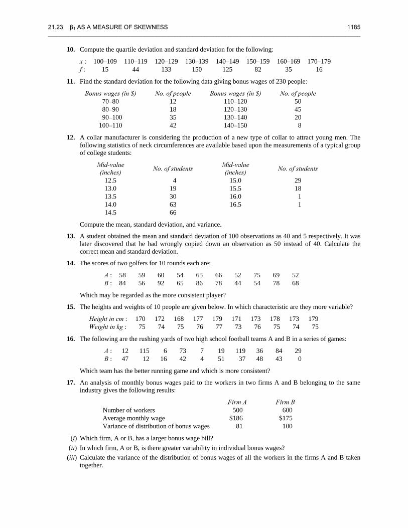
21.23 β1 AS A MEASURE OF SKEWNESS 1185 ________________________________________________________________________________________________________
10. Compute the quartile deviation and standard deviation for the following:
x : 100–109 110–119 120–129 130–139 140–149 150–159 160–169 170–179 f : 15 44 133 150 125 82 35 16
11. Find the standard deviation for the following data giving bonus wages of 230 people:
Bonus wages (in $) No. of people Bonus wages (in $) No. of people 70–80 12 110–120 50 80–90 18 120–130 45
90–100 35 130–140 20 100–110 42 140–150 8
12. A collar manufacturer is considering the production of a new type of collar to attract young men. The following statistics of neck circumferences are available based upon the measurements of a typical group of college students:
Mid-value (inches) No. of students Mid-value
(inches) No. of students
12.5 4 15.0 29 13.0 19 15.5 18 13.5 30 16.0 1 14.0 63 16.5 1 14.5 66
Compute the mean, standard deviation, and variance.
13. A student obtained the mean and standard deviation of 100 observations as 40 and 5 respectively. It was later discovered that he had wrongly copied down an observation as 50 instead of 40. Calculate the correct mean and standard deviation.
14. The scores of two golfers for 10 rounds each are:
A : 58 59 60 54 65 66 52 75 69 52 B : 84 56 92 65 86 78 44 54 78 68
Which may be regarded as the more consistent player?
15. The heights and weights of 10 people are given below. In which characteristic are they more variable?
Height in cm : 170 172 168 177 179 171 173 178 173 179 Weight in kg : 75 74 75 76 77 73 76 75 74 75
16. The following are the rushing yards of two high school football teams A and B in a series of games:
A : 12 115 6 73 7 19 119 36 84 29 B : 47 12 16 42 4 51 37 48 43 0
Which team has the better running game and which is more consistent?
17. An analysis of monthly bonus wages paid to the workers in two firms A and B belonging to the same industry gives the following results:
Firm A Firm B Number of workers 500 600 Average monthly wage $186 $175 Variance of distribution of bonus wages 81 100
(i) Which firm, A or B, has a larger bonus wage bill? (ii) In which firm, A or B, is there greater variability in individual bonus wages? (iii) Calculate the variance of the distribution of bonus wages of all the workers in the firms A and B taken
together.
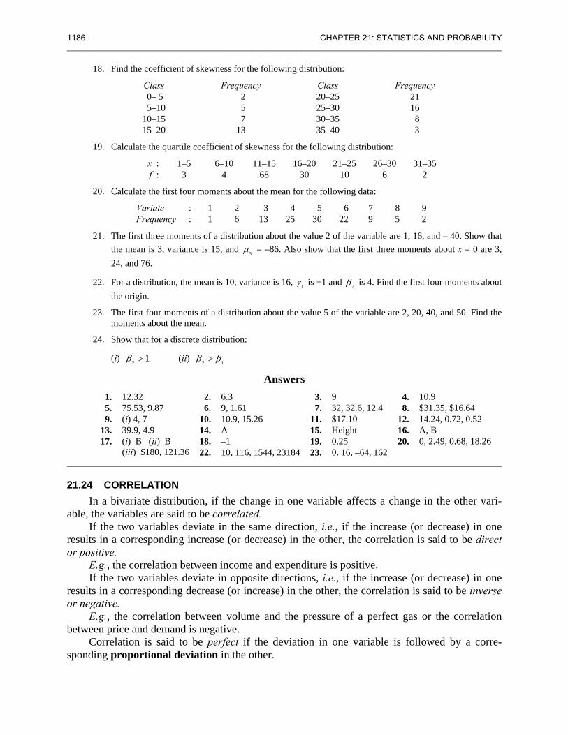
1186 CHAPTER 21: STATISTICS AND PROBABILITY ________________________________________________________________________________________________________
18. Find the coefficient of skewness for the following distribution:
Class Frequency Class Frequency 0– 5 2 20–25 21
5–10 5 25–30 16 10–15 7 30–35 8 15–20 13 35–40 3
19. Calculate the quartile coefficient of skewness for the following distribution:
x : 1–5 6–10 11–15 16–20 21–25 26–30 31–35 f : 3 4 68 30 10 6 2
20. Calculate the first four moments about the mean for the following data:
Variate : 1 2 3 4 5 6 7 8 9 Frequency : 1 6 13 25 30 22 9 5 2
21. The first three moments of a distribution about the value 2 of the variable are 1, 16, and – 40. Show that the mean is 3, variance is 15, and 3μ = –86. Also show that the first three moments about x = 0 are 3, 24, and 76.
22. For a distribution, the mean is 10, variance is 16, 1γ is +1 and 2β is 4. Find the first four moments about the origin.
23. The first four moments of a distribution about the value 5 of the variable are 2, 20, 40, and 50. Find the moments about the mean.
24. Show that for a discrete distribution:
(i) 2 1β > (ii) 2 1β β>
Answers 1. 12.32 2. 6.3 3. 9 4. 10.9 5. 75.53, 9.87 6. 9, 1.61 7. 32, 32.6, 12.4 8. $31.35, $16.64 9. (i) 4, 7 10. 10.9, 15.26 11. $17.10 12. 14.24, 0.72, 0.52
13. 39.9, 4.9 14. A 15. Height 16. A, B 17. (i) B (ii) B
(iii) $180, 121.36 18. –1 19. 0.25 20. 0, 2.49, 0.68, 18.26
22. 10, 116, 1544, 23184 23. 0. 16, –64, 162 ________________________________________________________________________________________________________
21.24 CORRELATION In a bivariate distribution, if the change in one variable affects a change in the other vari-
able, the variables are said to be correlated. If the two variables deviate in the same direction, i.e., if the increase (or decrease) in one
results in a corresponding increase (or decrease) in the other, the correlation is said to be direct or positive.
E.g., the correlation between income and expenditure is positive. If the two variables deviate in opposite directions, i.e., if the increase (or decrease) in one
results in a corresponding decrease (or increase) in the other, the correlation is said to be inverse or negative.
E.g., the correlation between volume and the pressure of a perfect gas or the correlation between price and demand is negative.
Correlation is said to be perfect if the deviation in one variable is followed by a corre-sponding proportional deviation in the other.
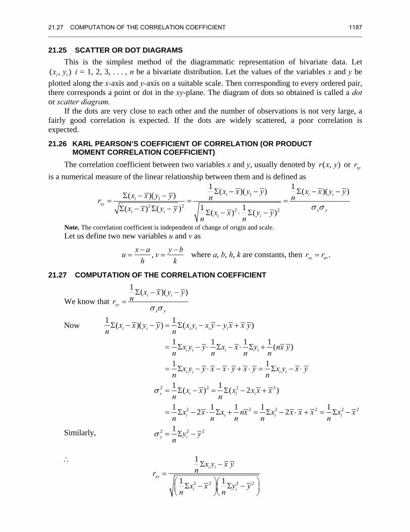
21.27 COMPUTATION OF THE CORRELATION COEFFICIENT 1187 ________________________________________________________________________________________________________
21.25 SCATTER OR DOT DIAGRAMS This is the simplest method of the diagrammatic representation of bivariate data. Let
( , )i ix y i = 1, 2, 3, . . . , n be a bivariate distribution. Let the values of the variables x and y be plotted along the x-axis and y-axis on a suitable scale. Then corresponding to every ordered pair, there corresponds a point or dot in the xy-plane. The diagram of dots so obtained is called a dot or scatter diagram.
If the dots are very close to each other and the number of observations is not very large, a fairly good correlation is expected. If the dots are widely scattered, a poor correlation is expected.
21.26 KARL PEARSON’S COEFFICIENT OF CORRELATION (OR PRODUCT MOMENT CORRELATION COEFFICIENT)
The correlation coefficient between two variables x and y, usually denoted by ( , )r x y or xyr is a numerical measure of the linear relationship between them and is defined as
1
12 2
2 2
1 1( )( ) ( )( )( )( )1 1( ) ( ) ( ) ( )
i i ii
xyx yi i
i i
x x y y x x y yx x y y n nrx x y y x x y y
n nσ σ
Σ − − Σ − −Σ − −= = =
Σ − Σ − Σ − ⋅ Σ −
Note. The correlation coefficient is independent of change of origin and scale. Let us define two new variables u and v as
,x a y bu vh k− −
= = where a, b, h, k are constants, then .xy uvr r=
21.27 COMPUTATION OF THE CORRELATION COEFFICIENT
We know that
1 ( )( )i i
xyx y
x x y ynr
σ σ
Σ − −=
Now
Similarly,
2 2 2 2
2 2 2 2 2 2
2 2 2
1 1( )( ) ( )
1 1 1 1 ( )
1 1
1 1( ) ( 2 )
1 1 1 1 12 2
1
i i i i i i
i i i i
i i i i
x i i i
i i i i
y i
x x y y x y x y y x x yn n
x y y x x y nx yn n n n
x y y x x y x y x y x yn n
x x x x x xn n
x x x nx x x x x x xn n n n n
y yn
σ
σ
Σ − − = Σ − − +
= Σ − ⋅ Σ − ⋅ Σ +
= Σ − ⋅ − ⋅ + ⋅ = Σ − ⋅
= Σ − = Σ − +
= Σ − ⋅ Σ + = Σ − ⋅ + = Σ −
= Σ −
∴
2 2 2 2
1
1 1
i i
xy
i i
x y x ynr
x x y yn n
Σ −=
⎛ ⎞⎛ ⎞Σ − Σ −⎜ ⎟⎜ ⎟⎝ ⎠⎝ ⎠
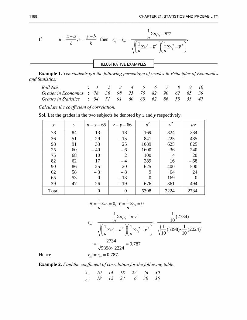
1188 CHAPTER 21: STATISTICS AND PROBABILITY ________________________________________________________________________________________________________
If 2 2 2 2
1
, then .1 1
i i
xy uv
i i
u v u vx a y b nu v r rh k
u u v vn n
Σ −− −= = = =
⎛ ⎞⎛ ⎞Σ − Σ −⎜ ⎟⎜ ⎟⎝ ⎠⎝ ⎠
Example 1. Ten students got the following percentage of grades in Principles of Economics and Statistics:
Roll Nos. : 1 2 3 4 5 6 7 8 9 10 Grades in Economics : 78 36 98 25 75 82 90 62 65 39 Grades in Statistics : 84 51 91 60 68 62 86 58 53 47
Calculate the coefficient of correlation.
Sol. Let the grades in the two subjects be denoted by x and y respectively.
x y u = x – 65 v = y – 66 u2 v2 uv 78 84 13 18 169 324 234 36 51 – 29 – 15 841 225 435 98 91 33 25 1089 625 825 25 60 – 40 – 6 1600 36 240 75 68 10 2 100 4 20 82 62 17 – 4 289 16 – 68 90 86 25 20 625 400 500 62 58 – 3 – 8 9 64 24 65 53 0 – 13 0 169 0 39 47 –26 – 19 676 361 494
Total 0 0 5398 2224 2734
Hence
2 2 2 2
1 10, 0
1 1 (2734)10
1 11 1 (5398) (2224)10 10
2734 0.7875398 2224
0.787.
i i
i i
uv
i i
xy uv
u u v vn n
u v u vnr
u u v vn n
r r
= Σ = = Σ =
Σ −= =
⎛ ⎞⎛ ⎞ ⋅Σ − Σ −⎜ ⎟⎜ ⎟⎝ ⎠⎝ ⎠
= =×
= =
Example 2. Find the coefficient of correlation for the following table:
x : 10 14 18 22 26 30 y : 18 12 24 6 30 36
ILLUSTRATIVE EXAMPLES
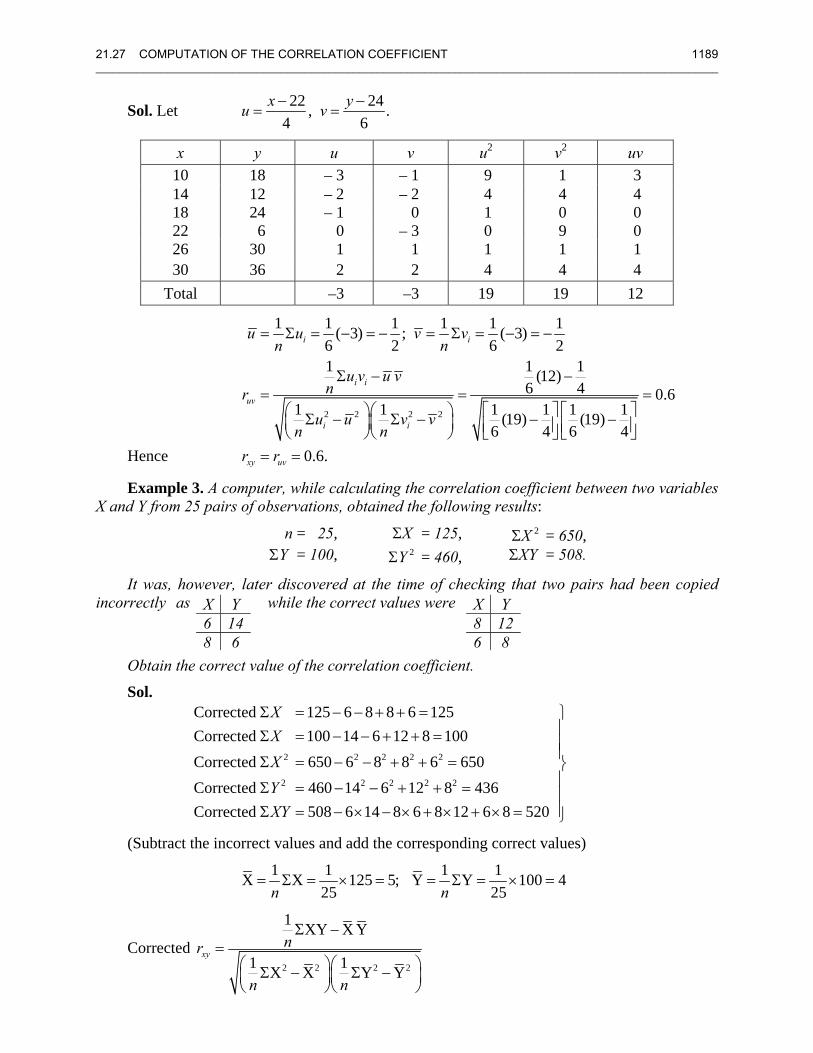
X Y 6 14 8 6
X Y 8 126 8
21.27 COMPUTATION OF THE CORRELATION COEFFICIENT 1189 ________________________________________________________________________________________________________
Sol. Let 22 24, .4 6
x yu v− −= =
x y u v u2 v2 uv 10 18 – 3 – 1 9 1 3 14 12 – 2 – 2 4 4 4 18 24 – 1 0 1 0 0 22 6 0 – 3 0 9 0 26 30 1 1 1 1 1 30 36 2 2 4 4 4
Total –3 –3 19 19 12
Hence
2 2 2 2
1 1 1 1 1 1( 3) ; ( 3)6 2 6 21 1 1(12)
6 4 0.61 1 1 1 1 1(19) (19)
6 4 6 40.6.
i i
i i
uv
i i
xy uv
u u v vn n
u v u vnr
u u v vn n
r r
= Σ = − = − = Σ = − = −
Σ − −= = =
⎛ ⎞⎛ ⎞ ⎡ ⎤ ⎡ ⎤Σ − Σ − − −⎜ ⎟⎜ ⎟ ⎢ ⎥ ⎢ ⎥⎝ ⎠⎝ ⎠ ⎣ ⎦ ⎣ ⎦= =
Example 3. A computer, while calculating the correlation coefficient between two variables X and Y from 25 pairs of observations, obtained the following results:
n = 25, XΣ = 125, 2XΣ = 650, YΣ = 100, 2YΣ = 460, XYΣ = 508.
It was, however, later discovered at the time of checking that two pairs had been copied incorrectly as while the correct values were
Obtain the correct value of the correlation coefficient.
Sol.
2 2 2 2 2
2 2 2 2 2
Corrected 125 6 8 8 6 125Corrected 100 14 6 12 8 100Corrected 650 6 8 8 6 650Corrected 460 14 6 12 8 436Corrected 508 6 14 8 6 8 12 6 8 520
XXXYXY
Σ = − − + + = ⎫⎪Σ = − − + + = ⎪⎪Σ = − − + + = ⎬⎪Σ = − − + + = ⎪⎪Σ = − × − × + × + × = ⎭
(Subtract the incorrect values and add the corresponding correct values)
1 1 1 1X X 125 5; Y Y 100 425 25n n
= Σ = × = = Σ = × =
Corrected 2 2 2 2
1 XY X Y
1 1X X Y Yxy
nr
n n
Σ −=
⎛ ⎞⎛ ⎞Σ − Σ −⎜ ⎟⎜ ⎟⎝ ⎠⎝ ⎠
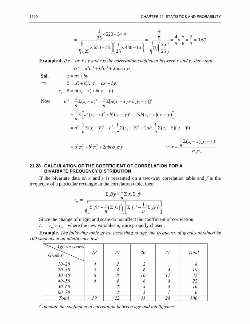
1190 CHAPTER 21: STATISTICS AND PROBABILITY ________________________________________________________________________________________________________
1 4520 5 4 4 5 225 5 0.67.5 6 31 1 36650 25 436 16 (1)
25 25 25
× − ×= = = × = =
⎛ ⎞⎛ ⎞ ⎛ ⎞× − × −⎜ ⎟⎜ ⎟ ⎜ ⎟⎝ ⎠⎝ ⎠ ⎝ ⎠
Example 4. If z = ax + by and r is the correlation coefficient between x and y, show that 2 2 2 2 2 2 .z x y x ya b abrσ σ σ σ σ= + +
Sol.
2 2 2
2 2 2 2
2 2 2 2
2 2 2 2
,( ) ( )
1 1( ) [ ( ) ( )]
1 ( ) ( ) 2 ( )( )
1 1 1( ) ( ) 2 ( )( )
1 (2
i i i
i i i
z i i i
i i i i
i i i i
x y x
z ax byz ax by z ax by
z z a x x b y y
z z a x x b y yn n
a x x b y y ab x x y yn
a x x b y y ab x x y yn n n
na b abr y r
σ
σ σ σ σ
= += + = +
− = − + −
= Σ − = Σ − + −
⎡ ⎤= Σ − + − + − −⎣ ⎦
= ⋅ Σ − + ⋅ Σ − + ⋅ Σ − −
Σ= + + =∵
)( )i i
x y
x x y y
σ σ
− −
⇒
Now
21.28 CALCULATION OF THE COEFFICIENT OF CORRELATION FOR A BIVARIATE FREQUENCY DISTRIBUTION
If the bivariate data on x and y is presented on a two-way correlation table and f is the frequency of a particular rectangle in the correlation table, then
( ) ( )2 22 2
1
1 1xy
fxy fx fynr
fx fx fy fyn n
Σ − Σ Σ=
⎡ ⎤ ⎡ ⎤Σ − Σ Σ − Σ⎢ ⎥ ⎢ ⎥⎣ ⎦ ⎣ ⎦
Since the change of origin and scale do not affect the coefficient of correlation, xy uvr r∴ = where the new variables u, v are properly chosen.
Example. The following table gives, according to age, the frequency of grades obtained by 100 students in an intelligence test:
Age (in years)
Grades 18 19 20 21 Total
10–20 4 2 2 8 20–30 5 4 6 4 19 30–40 6 8 10 11 35 40–50 4 4 6 8 22 50–60 2 4 4 10 60–70 2 3 1 6 Total 19 22 31 28 100
Calculate the coefficient of correlation between age and intelligence.
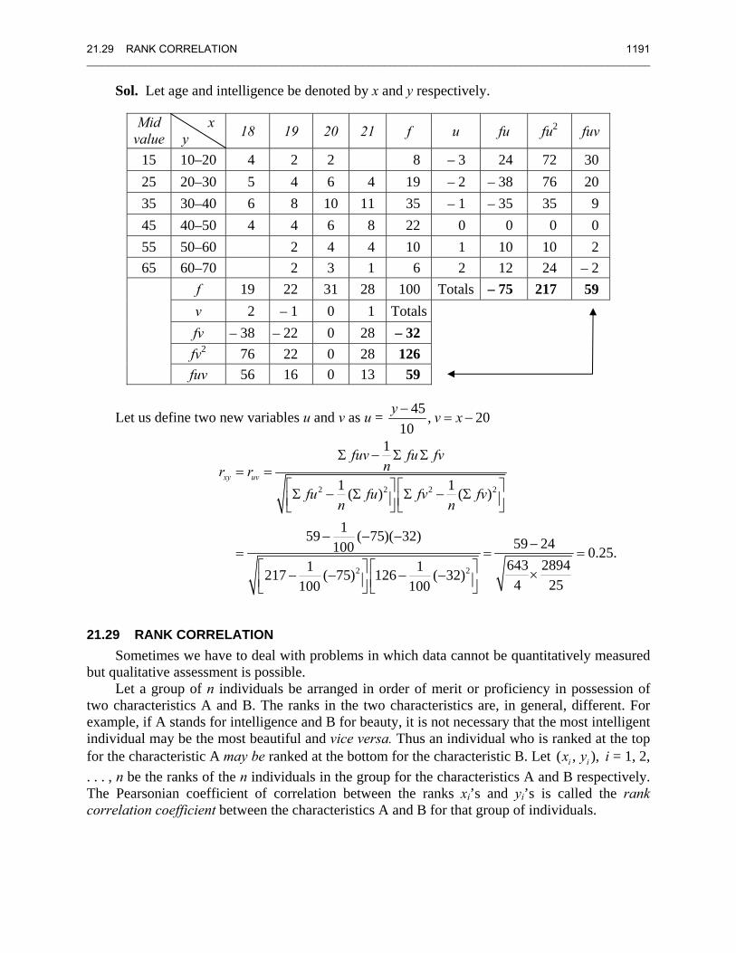
21.29 RANK CORRELATION 1191 ________________________________________________________________________________________________________
Sol. Let age and intelligence be denoted by x and y respectively.
Mid value
x 18 19 20 21 f u fu fu2 fuv y 15 10–20 4 2 2 8 – 3 24 72 30 25 20–30 5 4 6 4 19 – 2 – 38 76 20 35 30–40 6 8 10 11 35 – 1 – 35 35 9 45 40–50 4 4 6 8 22 0 0 0 0 55 50–60 2 4 4 10 1 10 10 2 65 60–70 2 3 1 6 2 12 24 – 2 f 19 22 31 28 100 Totals – 75 217 59 v 2 – 1 0 1 Totals fv – 38 – 22 0 28 – 32 fv2 76 22 0 28 126 fuv 56 16 0 13 59
Let us define two new variables u and v as u = 45 , 2010
y v x−= −
2 2 2 2
2 2
1
1 1( ) ( )
159 ( 75)( 32) 59 24100 0.25.643 28941 1217 ( 75) 126 ( 32)4 25100 100
xy uv
fuv fu fvnr r
fu fu fv fvn n
Σ − Σ Σ= =
⎡ ⎤ ⎡ ⎤Σ − Σ Σ − Σ⎢ ⎥ ⎢ ⎥⎣ ⎦ ⎣ ⎦
− − − −= = =
⎡ ⎤ ⎡ ⎤ ×− − − −⎢ ⎥ ⎢ ⎥⎣ ⎦ ⎣ ⎦
21.29 RANK CORRELATION Sometimes we have to deal with problems in which data cannot be quantitatively measured
but qualitative assessment is possible. Let a group of n individuals be arranged in order of merit or proficiency in possession of
two characteristics A and B. The ranks in the two characteristics are, in general, different. For example, if A stands for intelligence and B for beauty, it is not necessary that the most intelligent individual may be the most beautiful and vice versa. Thus an individual who is ranked at the top for the characteristic A may be ranked at the bottom for the characteristic B. Let ( , ),i ix y i = 1, 2, . . . , n be the ranks of the n individuals in the group for the characteristics A and B respectively. The Pearsonian coefficient of correlation between the ranks xi’s and yi’s is called the rank correlation coefficient between the characteristics A and B for that group of individuals.
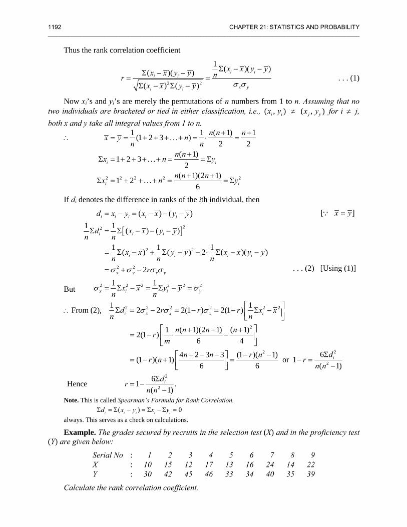
1192 CHAPTER 21: STATISTICS AND PROBABILITY ________________________________________________________________________________________________________
Thus the rank correlation coefficient
2 2
1 ( )( )( )( )( ) ( )
i ii i
x yi i
x x y yx x y y nrx x y y σ σ
Σ − −Σ − −= =
Σ − Σ − . . . (1)
Now xi’s and yi’s are merely the permutations of n numbers from 1 to n. Assuming that no two individuals are bracketed or tied in either classification, i.e., ( , )i ix y ≠ ( , )j yx y for i ≠ j, both x and y take all integral values from 1 to n.
∴
2 2 2 2 2
1 1 ( 1) 1(1 2 3 . . . )2 2
( 1)1 2 3 . . .2
( 1)(2 1)1 2 . . .6
i i
i i
n n nx y nn n
n nx n y
n n nx n y
+ += = + + + + = ⋅ =
+Σ = + + + + = = Σ
+ +Σ = + + + = = Σ
If di denotes the difference in ranks of the ith individual, then
[ ]22
2 2
2 2
2 2 2 2 2 2
( ) ( )1 1 ( ) ( )
1 1 1( ) ( ) 2 ( )( )
2
1 1
i i i i i
i i i
i i i i
x y x y
x i i y
d x y x x y y
d x x y yn n
x x y y x x y yn n n
r
x x y yn n
σ σ σ σ
σ σ
= − = − − −
Σ = Σ − − −
= Σ − + Σ − − ⋅ Σ − −
= + −
= Σ − = Σ − =
[ ]x y=∵
But
. . . (2) [Using (1)]
2 2 2 2 2 2
2
22
2
2
2
1 1From (2), 2 2 2(1 ) 2(1 )
1 ( 1)(2 1) ( 1)2(1 )6 4
64 2 3 3 (1 )( 1)(1 )( 1) or 16 6 ( 1)
6Hence 1 .( 1)
i x x x i
i
i
d r r r x xn n
n n n nrm
dn n r nr n rn n
drn n
σ σ σ ⎡ ⎤∴ Σ = − = − = − Σ −⎢ ⎥⎣ ⎦⎡ ⎤+ + +
= − ⋅ −⎢ ⎥⎣ ⎦
Σ+ − − − −⎡ ⎤= − + = − =⎢ ⎥ −⎣ ⎦Σ
= −−
Note. This is called Spearman’s Formula for Rank Correlation. ( ) 0i i i i id x y x yΣ = Σ − = Σ − Σ =
always. This serves as a check on calculations.
Example. The grades secured by recruits in the selection test (X) and in the proficiency test (Y) are given below:
Serial No : 1 2 3 4 5 6 7 8 9 X : 10 15 12 17 13 16 24 14 22 Y : 30 42 45 46 33 34 40 35 39
Calculate the rank correlation coefficient.
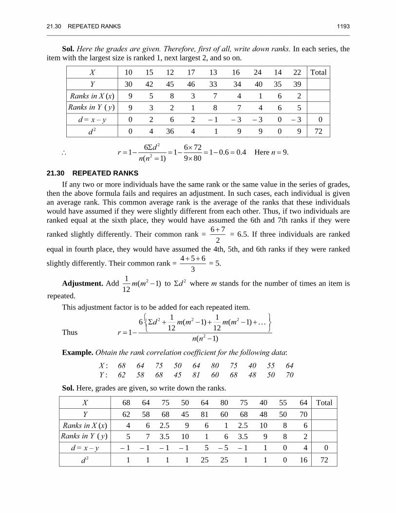
21.30 REPEATED RANKS 1193 ________________________________________________________________________________________________________
Sol. Here the grades are given. Therefore, first of all, write down ranks. In each series, the item with the largest size is ranked 1, next largest 2, and so on.
X 10 15 12 17 13 16 24 14 22 TotalY 30 42 45 46 33 34 40 35 39
Ranks in X (x) 9 5 8 3 7 4 1 6 2 Ranks in Y ( )y 9 3 2 1 8 7 4 6 5
d = x – y 0 2 6 2 – 1 – 3 – 3 0 – 3 0 2d 0 4 36 4 1 9 9 0 9 72
∴ 2
2
6 6 721 1 1 0.6 0.4 Here 9.( 1) 9 80
dr nn n
Σ ×= − = − = − = =
= ×
21.30 REPEATED RANKS If any two or more individuals have the same rank or the same value in the series of grades,
then the above formula fails and requires an adjustment. In such cases, each individual is given an average rank. This common average rank is the average of the ranks that these individuals would have assumed if they were slightly different from each other. Thus, if two individuals are ranked equal at the sixth place, they would have assumed the 6th and 7th ranks if they were
ranked slightly differently. Their common rank = 6 72+ = 6.5. If three individuals are ranked
equal in fourth place, they would have assumed the 4th, 5th, and 6th ranks if they were ranked
slightly differently. Their common rank = 4 5 63
+ + = 5.
Adjustment. Add 21 ( 1)12
m m − to 2dΣ where m stands for the number of times an item is
This adjustment factor is to be added for each repeated item.
Thus
2 2 2
2
1 16 ( 1) ( 1) . . .12 121
( 1)
d m m m mr
n n
⎧ ⎫Σ + − + − +⎨ ⎬⎩ ⎭= −
−
Example. Obtain the rank correlation coefficient for the following data:
X : 68 64 75 50 64 80 75 40 55 64 Y : 62 58 68 45 81 60 68 48 50 70
Sol. Here, grades are given, so write down the ranks.
X 68 64 75 50 64 80 75 40 55 64 Total Y 62 58 68 45 81 60 68 48 50 70
Ranks in X (x) 4 6 2.5 9 6 1 2.5 10 8 6 Ranks in Y ( )y 5 7 3.5 10 1 6 3.5 9 8 2
d = x – y – 1 – 1 – 1 – 1 5 – 5 – 1 1 0 4 0 2d 1 1 1 1 25 25 1 1 0 16 72
repeated.
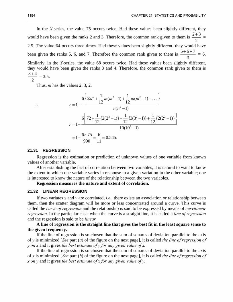
1194 CHAPTER 21: STATISTICS AND PROBABILITY ________________________________________________________________________________________________________
In the X-series, the value 75 occurs twice. Had these values been slightly different, they
would have been given the ranks 2 and 3. Therefore, the common rank given to them is 2 32+ =
2.5. The value 64 occurs three times. Had these values been slightly different, they would have
been given the ranks 5, 6, and 7. Therefore the common rank given to them is 5 6 73
+ + = 6.
Similarly, in the Y-series, the value 68 occurs twice. Had these values been slightly different, they would have been given the ranks 3 and 4. Therefore, the common rank given to them is 3 4
2+ = 3.5.
Thus, m has the values 2, 3, 2.
∴
2 2 2
2
2 2 2
2
1 16 ( 1) ( 1) . . .12 121
( 1)1 1 16 72 {2(2 1)} {3(3 1)} {2(2 1)}
12 12 12110(10 1)
6 75 61 0.545.990 11
d m m m mr
n n
r
⎧ ⎫Σ + − + − +⎨ ⎬⎩ ⎭= −
−
⎡ ⎤+ − + − + −⎢ ⎥⎣ ⎦= −−
×= − = =
21.31 REGRESSION Regression is the estimation or prediction of unknown values of one variable from known
values of another variable. After establishing the fact of correlation between two variables, it is natural to want to know
the extent to which one variable varies in response to a given variation in the other variable; one is interested to know the nature of the relationship between the two variables.
Regression measures the nature and extent of correlation.
21.32 LINEAR REGRESSION If two variates x and y are correlated, i.e., there exists an association or relationship between
them, then the scatter diagram will be more or less concentrated around a curve. This curve is called the curve of regression and the relationship is said to be expressed by means of curvilinear regression. In the particular case, when the curve is a straight line, it is called a line of regression and the regression is said to be linear.
A line of regression is the straight line that gives the best fit in the least square sense to the given frequency.
If the line of regression is so chosen that the sum of squares of deviation parallel to the axis of y is minimized [See part (a) of the figure on the next page], it is called the line of regression of y on x and it gives the best estimate of y for any given value of x.
If the line of regression is so chosen that the sum of squares of deviation parallel to the axis of x is minimized [See part (b) of the figure on the next page], it is called the line of regression of x on y and it gives the best estimate of x for any given value of y.
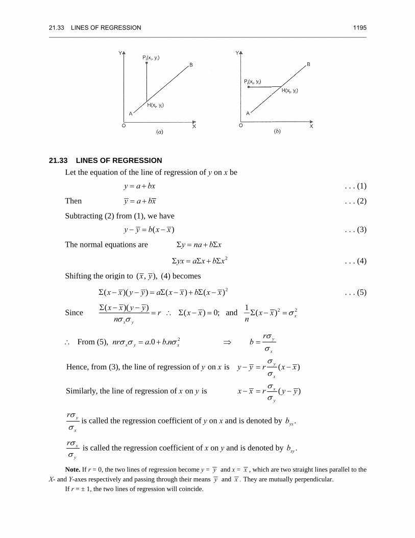
21.33 LIN__________
21.33 LLet
The
Sub
The
Shif
Sinc
F
Hen
Sim
∴
y
x
rσσ
x
y
rσσ
NoteX- and Y-a
If r =
NES OF REGR______________
LINES OF Rthe equation
n
tracting (2)
normal equ
fting the orig
(xΣ −
ce (xn
Σ −
From (5),
nce, from (3)
milarly, the lin
n
y is called th
x is called th
e. If r = 0, the txes respectivel
= ± 1, the two l
RESSION _____________
REGRESSIOn of the line
y a bx= +
y a bx= +
from (1), we
(y y b− =
uations are
gin to ( , )x y
)( )x y y− =
)( )
x y
x y ynσ σ− −
=
.0
), the line of
ne of regress
x yr aσ σ =
he regression
he regression
two lines of regly and passing lines of regress
______________
ON of regression
x
e have
)x x−
y nΣ =
yx aΣ =
, (4) becom
( )a x xΣ − +
(r x= ∴ Σ −
2.
f regression o
sion of on
xb n
x
σ+
n coefficient
n coefficient
gression becomthrough their m
sion will coinci
______________
n of y on x b
na b x+ Σ
2a x b xΣ + Σ
mes 2( )b x xΣ −
) 0; anx− =
of on is
is
y x
y
⇒
of y on x an
of x on y an
me y = y and xmeans y and ide.
_____________
be
1nd (x xn
Σ −
x
rb
y y r
x x r
σσσσσσ
=
− =
− =
d is denoted
nd is denoted
x = x , which ax . They are m
______________
2 2) xx σ=
( )
( )
y
x
y
x
x
y
x x
y y
σσσσ
−
−
d by .yxb
d by .xyb
are two straighmutually perpen
______________
.
.
.
.
.
ht lines parallelndicular.
1195 ______
. . (1)
. . (2)
. . (3)
. . (4)
. . (5)
l to the
1196 CHAPTER 21: STATISTICS AND PROBABILITY ________________________________________________________________________________________________________
21.34 PROPERTIES OF REGRESSION Property I. The correlation coefficient is the geometric mean between the regression
coefficients.
Proof. The coefficients of regression are y
x
rσσ
and .x
y
rσσ
G.M. between them 2y x
x y
r r r rσ σσ σ
= × = = = coefficient of correlation.
Property II. If one of the regression coefficients is greater than 1, the other must be less than 1.
Proof. The two regression coefficients are and .y xyx xy
x y
r rb bσ σσ σ
= =
Let 11, then 1yxyx
bb
> < . . . (1)
Since 2 11 ( 1 1) 1.xy xy xyyx
b b r r bb
⋅ = ≤ − ≤ ≤ ∴ ≤ <∵ | Using (1)
Similarly, if 1,xyb > then 1.yxb <
Property III. The arithmetic mean of regression coefficients is greater than the correlation coefficient.
Proof. We have to prove that or2 2
y x
yx xy x y
r rb b
r r
σ σσ σ
++
> >
or 2 2 22 or ( ) 0, which is true.y x x y x yσ σ σ σ σ σ+ > − > Property IV. Regression coefficients are independent of the origin but not of scale.
. Let , where , , , and are constants
Similarly, .
y v vyx vu
x u u
xy uv
x a y bu v a b h kh k
r k rk kb r bh h h
hb bk
σ σ σσ σ σ
− == =
⎛ ⎞= = ⋅ = =⎜ ⎟
⎝ ⎠
=
Proof
Thus, byx and bxy are both independent of a and b but not of h and k.
Property V. The correlation coefficient and the two regression coefficients have the same sign.
Proof. Regression coefficient of y on x = yxy
x
b rσσ
=
Regression coefficient of x on y = xxy
y
b r σσ
=
Since xσ and yσ are both positive, , ,yx xyb b and r have the same sign.
21.35 ANGLE BETWEEN TWO LINES OF REGRESSION 1197 ________________________________________________________________________________________________________
21.35 ANGLE BETWEEN TWO LINES OF REGRESSION If θ is the acute angle between the two regression lines in the case of two variables x and y,
show that
2
2 2
1tan x y
x y
rr
σ σθ
σ σ−
= ⋅+
where r, ,x yσ σ have their usual meanings.
Explain the significance of the formula when r = 0 and r = ± 1. Proof. Equations of the lines of regression of y on x and x on y are
( ) and ( )y x
x y
r ry y x x x x y yσ σσ σ
− = − − = −
Their slopes are 1 2and .y y
x x
rm m
rσ σσ σ
= =
∴ 2 12
2 12
22 2
2 2 2 2
tan1
1
1 1
y y
x x
y
x
y x yx
x x y x y
rrm m
m m
r rr r
σ σσ σθ
σσ
σ σ σσσ σ σ σ σ
−−
= ± = ±+
+
− −= ± ⋅ ⋅ = ± ⋅
+ +
Since 2 1r ≤ and ,x yσ σ are positive. ∴ Positive sign gives the acute angle between the lines.
Hence 2
2 2
1tan x y
x y
rr
σ σθ
σ σ−
= ⋅+
when 0,2
r πθ= =
∴ The two lines of regression are perpendicular to each other. Hence the estimated value of y is the same for all values of x and vice versa when r = ± 1,
tan θ = 0 so that, θ = 0 or .π Hence the lines of regression coincide and there is a perfect correlation between the two
variates x and y.
Note. 22 2
1 1 1
1x x
y x y y y
xy x y xy x y xy x yr n n n
y yn
σ σσ σ σ σ σ
Σ − Σ − Σ −= ⋅ = =
Σ −
Similarly, 2 2
1
.1y
x
xy x yr n
x xn
σσ
Σ −=
Σ −
1198 CHAPTER 21: STATISTICS AND PROBABILITY ________________________________________________________________________________________________________
Example 1. Calculate the coefficient of correlation and obtain the least square regression line of y on x for the following data:
x : 1 2 3 4 5 6 7 8 9 y : 9 8 10 12 11 13 14 16 15
Also obtain an estimate of y that should correspond on the average to x = 6.2.
Sol.
x y u = x – 5 u = y – 12 u2 v2 uv 1 9 – 4 – 3 16 9 12 2 8 – 3 – 4 9 16 12 3 10 – 2 – 2 4 4 4 4 12 – 1 0 1 0 0 5 11 0 – 1 0 1 0 6 13 1 1 1 1 1 7 14 2 2 4 4 4 8 16 3 4 9 16 12 9 15 4 3 16 9 12
Total 0 0 60 60 57
Also
2 2 2 2
2 2
1 1 (57) 09
1 1 1 1(60) 0 (60) 09 9
19 0.9520
1 1 (57) 0 199 0.951 1 20(60) 09
1 15 5, 12 129 9
xy uv
y v
x u
uv u vnr r
u u v vn n
uv u vr r n
u un
x u y v
σ σσ σ
Σ − −= = =
⎛ ⎞⎛ ⎞ ⎡ ⎤ ⎡ ⎤Σ − Σ − − −⎜ ⎟⎜ ⎟ ⎢ ⎥ ⎢ ⎥⎝ ⎠⎝ ⎠ ⎣ ⎦ ⎣ ⎦
= =
Σ − −= = = = =
Σ − −
= + Σ = = + Σ =
Equation of the line of regression of y on x is
( )
or 12 0.95( 5)or 0.95 7.25
y
x
ry y x x
y xy x
σσ
− = −
− = −= +
When x = 6.2, the estimated value of y = 0.95 × 6.2 + 7.25 = 5.89 + 7.25 = 13.14.
ILLUSTRATIVE EXAMPLES
21.35 ANGLE BETWEEN TWO LINES OF REGRESSION 1199 ________________________________________________________________________________________________________
Example 2. In a partially destroyed laboratory record of an analysis of a correlation data, only the following results are legible:
Variance of x = 9 Regression equations: 8x – 10y + 66 = 0, 40x – 18y = 214. What were (a) the mean values of x and y, (b) the standard deviation of y, and (c) the
coefficient of correlation between x and y. Sol. (i) Since both the lines of regression pass through the point ( , )x y therefore, we
have
8 10 66 040 18 214 040 50 330 0
32 544 08 170 66 0 or
13,
x yx yx y
yx
x
− + =− − =− + =
− = ∴− + =
=
178 104 13
17
yx xy
== ∴ ==
. . . (1) . . . (2)Multiplying (1) by 5, . . . (3)
Subtracting (3) from (2),
∴ From (1),
Hence . . . (a)( ) Variance ofii∴
2 9
3x
x
x σσ
= ==
(given)
The equations of the lines of regression can be written as
.8 6.6 and .45 5.35y x x y= + = +
∴ The regression coefficient of y on x is .8y
x
rσσ
= . . . (4)
The regression coefficient of x on y is .45x
y
rσσ
= . . . (5)
Multiplying (4) and (5), 2 .8 .45 .36 0.6r r= × = ∴ = . . . (b)
(Positive sign with square root is taken because regression coefficients are positive.)
From (4), .8 .8 3 4.0.6
xy r
σσ ×= = = . . . (c)
1. (a) Calculate the correlation coefficient for the following heights in inches of fathers (X) and their sons ( )Y .
X : 65 66 67 67 68 69 70 72 Y : 67 68 65 68 72 72 69 71
(b) Find the correlation coefficient between x and y from the given data:
x : 78 89 97 69 59 79 68 57 y : 125 137 156 112 107 138 123 108
(c) Find the correlation coefficient from the following data:
x : 92 89 87 86 83 77 71 63 53 50 y : 86 88 91 77 68 85 52 82 37 57
TEST YOUR KNOWLEDGE
1200 CHAPTER 21: STATISTICS AND PROBABILITY ________________________________________________________________________________________________________
2. Calculate the coefficient of correlation for the following ages of husbands and wives:
Husbands’s age x : 23 27 28 28 29 30 31 33 35 36 Wife’s age y : 18 20 22 27 21 29 27 29 28 29
3. Establish the formula 2 2 2 2x y x y x yrσ σ σ σ σ−
= + −
where r is the correlation coefficient between x and y.
4. (a) Calculate the coefficient of correlation for the following table:
x 16–18 18–20 20–22 22–24 y
10–20 2 1 1
20–30 3 2 3 2
30–40 3 4 5 6
40–50 2 2 3 4
50–60 1 2 2
60–70 1 2 1
(b) Find the correlation between x (grades in mathematics) and y (grades in Engineering Drawing) given in the following data:
x 10–40 40–70 70–100 Total y
0–30 5 20 — 25 30–60 — 28 2 30 60–90 — 32 13 45 Total 5 80 15 100
5. Ten students got the following percentage of grades in chemistry and physics:
Students : 1 2 3 4 5 6 7 8 9 10 Grades in chemistry : 78 36 98 25 75 82 90 62 65 39 Grades in physics : 84 51 91 60 68 62 86 58 63 47
Calculate the rank correlation coefficient.
6. Ten competitors in a musical test were ranked by the three judges x, y, and z in the following order:
Ranks by x : 1 6 5 10 3 2 4 9 7 8 Ranks by y : 3 5 8 4 7 10 2 1 6 9 Ranks by z : 6 4 9 8 1 2 3 10 5 7
Using the rank correlation method, discuss which pair of judges has the nearest approach to common likings in music.
7. A sample of 12 fathers and their sons gave the following data about their heights in inches:
Father : 65 63 67 64 68 62 70 66 68 67 69 71 Son : 68 66 68 65 69 66 68 65 71 67 68 70
Calculate the coefficient of rank correlation.
8. If r = 0, show that the two lines of regression are parallel to the axes.
9. If the two regression coefficients are 0.8 and 0.2, what would be the value of the coefficient of correlation?
21.36 THEORY OF PROBABILITY 1201 ________________________________________________________________________________________________________
10. (a) Find the correlation coefficient and the equations of regression lines for the following values of x and y:
x : 1 2 3 4 5 y : 2 5 3 8 7
(b) Find the correlation coefficient between x and y for the given values. Find also the two regression lines.
x : 1 2 3 4 5 6 7 8 9 10 y : 10 12 16 28 25 36 41 49 40 50
11. The two regression equations of the variables x and y are x = 19.13 – 0.87y and y = 11.64 – 0.50x. Find
(i) mean of x’s, (ii) mean of y’s, and (iii) the correlation coefficient between x and y. 12. Two random variables have the regression lines with equations 3x + 2y = 26 and 6x + y = 31. Find the
mean values and the correlation coefficient between x and y. 13. In a partially destroyed sheet of laboratory data, only the equations giving the two lines of regression of
y on x and x on y are available and are respectively, 7x – 16y + 9 = 0, 5y – 4x – 3 = 0. Calculate the coefficient of correlation, x and y .
Answers
1. (a) 0.603 (b) 0.96 (e) 0.7291 2. 0.82 4. (a) 0.28 (b) 0.4517 5. 0.84 6. x and z 7. 0.722 9. 0.4 10. (a) r = 0.8; y = 1.3x + 1.1; x = 0.5y + 0.5
(b) r = 0.96; y = 4.69x + 4.9; x = 0.2y – 0.64 11. (i) 15.79 (ii) 3.74 (iii) –0.6595 12. 4, 7; 0.5x y r= = − 13. 0.7395; 0.1034; 0.5172.r x y= = − =
________________________________________________________________________________________________________
21.36 THEORY OF PROBABILITY Here we define and explain certain terms that are used frequently. (a) Trial and event. Let an experiment be repeated under essentially the same conditions
and let it result in any one of the several possible outcomes. Then, the experiment is called a trial and the possible outcomes are known as events or cases.
For example: (i) Tossing a coin is a trial and the turning up of heads or tails is an event. (ii) Throwing a die is a trial and getting 1 or 2 or 3 or 4 or 5 or 6 is an event. (b) Exhaustive events. The total number of all possible outcomes in any trial is known as
exhaustive events or exhaustive cases. For example: (i) In tossing a coin, there are two exhaustive cases, heads and tails. (ii) In throwing a die, there are 6 exhaustive cases, for any one of the six faces that may
turn up. (iii) In throwing two dice, the exhaustive cases are 6 × 6 = 62, for any of the 6 numbers
from 1 to 6 on one die can be associated with any of the 6 numbers on the other die. In general, in throwing n dice, the exhaustive cases are 6n. (c) Favorable events or cases. The cases that entail the occurrence of an event are said to
be favorable to the event. It is the total number of possible outcomes in which the specified event happens.
For example: (i) In throwing a die, the number of cases favorable to the appearance of a multiple of 3
are two, viz. 3 and 6, while the number of cases favorable to the appearance of an even number are three, viz., 2, 4, and 6.
1202 CHAPTER 21: STATISTICS AND PROBABILITY ________________________________________________________________________________________________________
(ii) In a throw of two dice, the number of cases favorable to getting a sum of 6 is 5, viz., (1, 5); (5, 1); (2,4); (4, 2); (3, 3).
(d) Mutually exclusive events. Events are said to be mutually exclusive or incompatible if the occurrence of any one of them precludes (i.e., rules out) the occurrence of all others, i.e., if no two or more than two of them can happen simultaneously in the same trial.
For example: (i) In tossing a coin, the events “heads” and “tails” are mutually exclusive, since if the
outcome is heads, the possibility of getting tails in the same trial is ruled out. (ii) In throwing a die, all the six faces numbered, 1, 2, 3, 4, 5, 6 are mutually exclusive
since any outcome rules out the possibility of getting any other. (e) Equally likely events. Events are said to be equally likely if there is no reason to expect
any one in preference to any other. For example: (i) When a card is drawn from a well-shuffled deck, any card may appear in the draw so
that the 52 different cases are equally likely. (ii) In throwing a die, all six faces are equally likely to come up. ( )f Independent and dependent events. Two or more events are said to be independent if
the occurrence or non-occurrence of any one does not depend (or is not affected) by the occurrence or non-occurrence of any other. Otherwise they are said to be dependent.
For example: If a card is drawn from a deck of well-shuffled cards and replaced before drawing the second card, the result of the second draw is independent of the first draw. However, if the first card drawn is not replaced, then the second draw is dependent on the first draw.
21.37 (a) MATHEMATICAL (OR CLASSICAL) DEFINITION OF PROBABILITY If a trial results in n exhaustive, mutually exclusive and equally likely cases and m of them
are favorable to the occurrence of an event E, then the probability of occurrence of E is given by
Favorable number of cases or P (E) .Exhaustive number of cases
mpn
= =
Note 1. Since the number of cases favorable to the occurrence of E is m and the exhaustive number of cases is n, therefore, the number of cases unfavorable to the occurrence of E are n – m.
Note 2. The probability that the event E will not happen is given by
Unfavorable number of cases
or P(E) 1 1Exhaustive number of cases
n m mq p
n n
−= = = − = −
Obviously, p and q are non-negative and cannot exceed 1, i.e., 0 1, 0 1.p q≤ ≤ ≤ ≤ Note 3. If P(E) = 1, E is called a certain event, i.e., the chance of its occurrence is 100%. If P(E) = 0, then E is an impossible event. Note 4. If n cases are favorable to E and m cases are favorable to E (i.e., unfavorable to E), then exhaustive
number of cases = n + m.
P(E) and P(E)n m
n m n m= =
+ +
We say that the “odds in favor of E” are n : m and the “odds against E” are m : n.
21.37 (b) STATISTICAL (OR EMPIRICAL) DEFINITION OF PROBABILITY If in n trials, an event E occurs m times, then the probability of the occurrence of E is given
by
P(E) Lt .n
mpn→∞
= =
21.37 (b) STATISTICAL (OR EMPIRICAL) DEFINITION OF PROBABILITY 1203 ________________________________________________________________________________________________________
Example 1. A bag contains 7 white, 6 red, and 5 black balls. Two balls are drawn at random. Find the probability that they will both be white.
Sol. Total number of balls = 7 + 6 + 5 = 18. Out of 18 balls, 2 can be drawn in 18C2 ways.
∴ Exhaustive number of cases = 18C2 = 18 172 1××
= 153
Out of 7 white balls, 2 can be drawn in 7C2 = 7 62 1××
= 21 ways.
∴ Favorable number of cases = 21
21 7Probability .153 51
= =
Example 2. Four cards are drawn from a deck of cards. Find the probability that (i) all are diamonds, (ii) there is one card of each suit, and (iii) there are two spades and two hearts.
Sol. 4 cards can be drawn from a deck of 52 cards in 52C4 ways.
∴ Exhaustive number of cases = 52C4 = 52 51 50 494 3 2 1× × ×× × ×
= 270725.
(i) There are 13 diamonds in the deck and 4 can be drawn out of them in 13C4 ways.
∴ Favorable number of cases = 13C4 = 13 12 11 104 3 2 1× × ×× × ×
= 715.
715 143 11Required probability .270725 54145 4165
= = =
(ii) There are 4 suits, each containing 13 cards. ∴ Favorable number of cases = 13CI × 13C1 × 13C1 × 13C1 = 13 × 13 × 13 × 13.
13 13 13 13 13 2197Required probability .270725 20825
× × × ×= =
(iii) 2 spades out of 13 can be drawn in 13C2 ways. 2 hearts out of 13 can be drawn in 13C2 ways. ∴ Favorable number of cases = 13C2 × 13C2 = 78 × 78
78 78 468Required probability .270725 20825
×= =
Example 3. A bag contains 50 tickets numbered 1, 2, 3, . . . , 50, of which five are drawn at random and arranged in ascending order of magnitude (x1 < x2 < x3 < x4 < x5). What is the probability that x3 = 30?
Sol. Exhaustive number of cases 50C5. If x3 = 30, then the two tickets with numbers x1 and x2 must come out of 29 tickets
numbered 1 to 29 and this can be done in 29C2 ways. The other two tickets with numbers x4 and x5 must come out of the 20 tickets number 31 to 50 and this can be done in 20C2 ways.
∴ Favorable number of cases = 29C2 × 20C2.
29 20
2 250
5
C C 551Required probability .C 15134×
= =
ILLUSTRATIVE EXAMPLES
1204 CHAPTER 21: STATISTICS AND PROBABILITY ________________________________________________________________________________________________________
21.38 RANDOM EXPERIMENT Occurrences that can be repeated a number of times, essentially under the same conditions,
and whose result cannot be predicted beforehand are known as random experiments. For example, the rolling of a die, or the tossing of a coin are random experiments. Sample Space. Out of the several possible outcomes of a random experiment, one and only
one can take place in a trial. The set of all these possible outcomes is called the sample space for the particular experiment and is denoted by S.
For example, if a coin is tossed, the possible outcomes are H (Heads) and T (Tails). Thus S = {H, T}. Sample Point. The elements of S, the sample space, are called sample points. For example, if a coin is tossed and H and T denote “Heads” and “Tails” respectively, then
S = {H, T}. The two sample points are H and T. Finite Sample Space. If the number of sample points in a sample space is finite, we call it a
finite sample space. (In this chapter, we shall deal with finite sample spaces only.) Event. Every subset of S, the sample space, is called an event. Since S ⊂ S, S itself is an event; called a certain event. Also, S,φ ⊂ the null set is also an event, called an impossible event. If e ∈ S, then e is called an elementary event. Every elementary event contains only one
sample point.
21.39 AXIOMS (i) With each event E (i.e., a sample point) is associated a real number between 0 and 1,
called the probability of that event and is denoted by P(E). Thus 0 ≤ P(E) ≤ 1. (ii) The sum of the probabilities of all simple (elementary) events constituting the sample
space is 1. Thus P(S) = 1. (iii) The probability of a compound event (i.e., an event made up of two or more sample
events) is the sum of the probabilities of the simple events comprising the compound event. Thus, if there are n equally likely possible outcomes of a random experiment, then the
sample space S contains n sample points and the probability associated with each sample point is
1 .n
[By Axiom (ii)]
Now, if an event E consists of m sample points, then the probability of E is
1 1P(E) . . . . times
Number of sample points in E .Number of sample points in S
mmn n n
= + + + =
=
This closely agrees with the classical definition of probability.
21.40 PROBABILITY OF THE IMPOSSIBLE EVENT IS ZERO, i.e., P (φ ) = 0
Impossible event contains no sample point. As such, the sample space S and the impossible event φ are mutually exclusive.
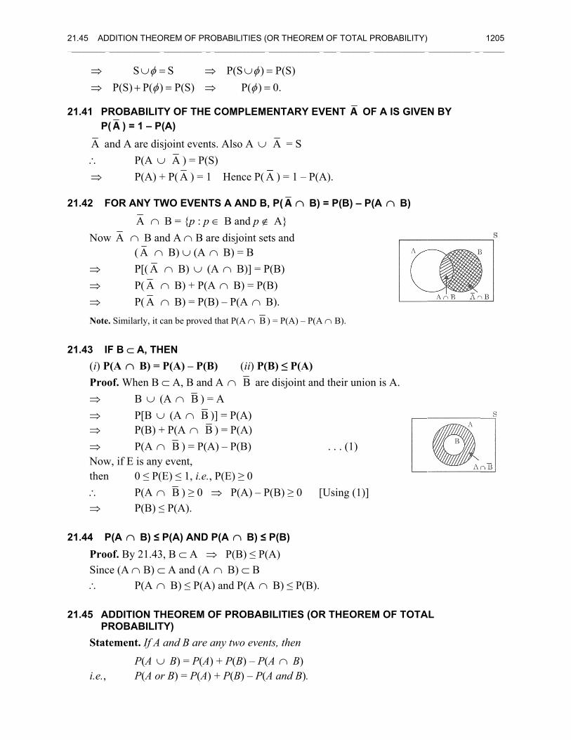
21.45 AD__________
⇒⇒
21.41 PP
A a∴ ⇒
21.42 F
Now ⇒ ⇒ ⇒ Note
21.43 I(i) PPro⇒ ⇒ ⇒ ⇒ Nowthen∴ ⇒
21.44 PProSinc∴
21.45 AP
Stat
i.e.,
DDITION THEO______________
SP(S) P( )
φφ
∪ =+
PROBABILITP(A ) = 1 – P
and A are disP(A ∪P(A) +
FOR ANY TW
A ∩w A ∩ B an
( A ∩P[( AP( A P( A
e. Similarly, it c
F B ⊂ A, THP(A ∩ B) = of. When B
B ∪ P[B ∪P(B) +P(A ∩
w, if E is anyn 0 ≤ P(
P(A ∩P(B) ≤
P(A ∩ B) ≤ of. By 21.43ce (A ∩ B) ⊂
P(A ∩
ADDITION TPROBABILITtement. If A
P(A ∪P(A o
OREM OF PRO_____________
S) P(S)φ= ⇒= ⇒
TY OF THE P(A)
sjoint events∪ A ) = P(S+ P( A ) = 1
WO EVENT
B = {p : p ∈nd A ∩ B ar∩ B) ∪ (A ∩
∩ B) ∪ (A∩ B) + P(A∩ B) = P(Bcan be proved
HEN P(A) – P(B⊂ A, B and (A ∩ B ) = ∪ (A ∩ B )+ P(A ∩ B∩ B ) = P(Ay event, (E) ≤ 1, i.e., ∩ B ) ≥ 0 ⇒≤ P(A).
P(A) AND P3, B ⊂ A ⇒⊂ A and (A ∩ B) ≤ P(A)
HEOREM OTY) and B are a
∪ B) = P(A) r B) = P(A)
OBABILITIES (______________
P(S )P( )φφ
⇒ ∪ =⇒ =
COMPLEM
s. Also A ∪S)
Hence P( A
TS A AND B
∈ B and p ∉re disjoint se∩ B) = B A ∩ B)] = P
A ∩ B) = P(BB) – P(A ∩ B
that P(A ∩ B
B) (ii) P(A ∩ B areA
)] = P(A) ) = P(A)
A) – P(B)
P(E) ≥ 0 ⇒ P(A) – P
P(A ∩ B) ≤⇒ P(B) ≤ P(∩ B) ⊂ B ) and P(A ∩
OF PROBAB
any two even
+ P(B) – P(+ P(B) – P(A
OR THEOREM______________
P(S)0.
==
ENTARY EV
A = S
A ) = 1 – P(A
, P(A ∩ B)
∉ A} ets and
P(B) B) B). ) = P(A) – P(A
(B) ≤ P(A) e disjoint and
P(B) ≥ 0 [
P(B) (A)
∩ B) ≤ P(B).
BILITIES (OR
nts, then
(A ∩ B) A and B).
M OF TOTAL P_____________
VENT A OF
A).
= P(B) – P(
A ∩ B).
d their union
. . . (1)
[Using (1)]
R THEOREM
PROBABILITY)______________
F A IS GIVE
(A ∩ B)
n is A.
M OF TOTA
______________
N BY
AL
1205 ______
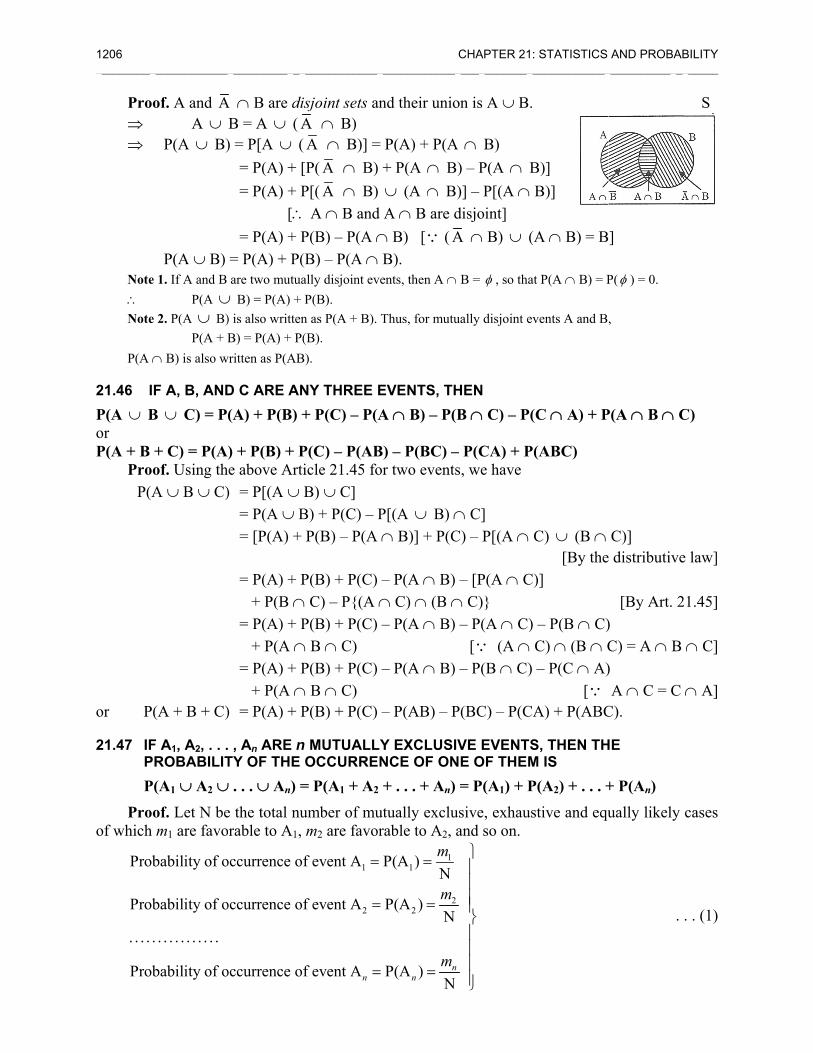
1206 __________
Pro⇒ ⇒ Note∴ Note P(A
21.46 IP(A ∪ Bor P(A + B
Pro P(A
or P
21.47 IFP
PPro
of which
Prob
Prob
. . . .
Prob
______________
of. A and AA ∪
P(A ∪ B)
P(A ∪ B) e 1. If A and B
P(A ∪e 2. P(A ∪ B)
P(A + B∩ B) is also w
F A, B, ANDB ∪ C) = P(
+ C) = P(A)of. Using thA ∪ B ∪ C)
(A + B + C)
F A1, A2, . . .PROBABILITP(A1 ∪ A2 ∪
of. Let N be m1 are favo
bability of o
bability of o
. . . . . . . . . . . .
bability of o
_____________
A ∩ B are disB = A ∪ ( A) = P[A ∪ (
= P(A) + [= P(A) + P [∴= P(A) + P
= P(A) + P(are two mutua
∪ B) = P(A) + ) is also writtenB) = P(A) + P(
written as P(AB
D C ARE AN(A) + P(B) +
) + P(B) + Pe above Arti) = P[(A ∪ B = P(A ∪ B = [P(A) + = P(A) + P + P(B ∩ = P(A) + P + P(A ∩ = P(A) + P + P(A ∩
) = P(A) + P
, An ARE nTY OF THE ∪ . . . ∪ An) =e the total nurable to A1,
occurrence of
occurrence of
occurrence of
______________
sjoint sets anA ∩ B) A ∩ B)] =
[P( A ∩ B) P[( A ∩ B) A ∩ B and
P(B) – P(A ∩(B) – P(A ∩ally disjoint eveP(B).
n as P(A + B). (B).
B).
NY THREE E+ P(C) – P(A
P(C) – P(ABicle 21.45 foB) ∪ C]
B) + P(C) – PP(B) – P(A
P(B) + P(C)∩ C) – P{(A ∩P(B) + P(C)∩ B ∩ C) P(B) + P(C)∩ B ∩ C) P(B) + P(C)
n MUTUALLYOCCURREN
= P(A1 + A2
umber of mum2 are favor
1
2
f event A
f event A
f event An
=
=
=
______________
nd their unio
= P(A) + P(A+ P(A ∩ B∪ (A ∩ BA ∩ B are d∩ B) [∵ ( AB). ents, then A ∩
Thus, for mutu
EVENTS, THA ∩ B) – P(
B) – P(BC) –or two events
P[(A ∪ B) ∩∩ B)] + P(C
– P(A ∩ B)∩ C) ∩ (B ∩– P(A ∩ B)
– P(A ∩ B)
– P(AB) – P
Y EXCLUSINCE OF ON+ . . . + An)
utually exclurable to A2, a
11
22
P(A )N
P(A )N
P(A )N
nn
m
m
m
=
= =
= =
CHAPTER 21_____________
on is A ∪ B.
A ∩ B) ) – P(A ∩ B)] – P[(A ∩disjoint] A ∩ B) ∪ (
B = φ , so tha
ually disjoint e
HEN B ∩ C) – P(
– P(CA) + Ps, we have
∩ C] C) – P[(A ∩
– [P(A ∩ C∩ C)}
– P(A ∩ C)[∵ (A ∩
– P(B ∩ C)
P(BC) – P(C
VE EVENTSNE OF THEM
= P(A1) + Pusive, exhausand so on. ⎫⎪⎪⎪⎪⎬⎪⎪⎪⎪⎭
: STATISTICS ______________
B)] B)]
(A ∩ B) = B
at P(A ∩ B) = P
vents A and B
(C ∩ A) + P
P(ABC)
C) ∪ (B ∩ [By the
C)]
) – P(B ∩ C)C) ∩ (B ∩ C – P(C ∩ A)
[∵ A) + P(ABC
S, THEN THM IS P(A2) + . . . +stive and equ
AND PROBAB______________
]
P(φ ) = 0.
,
P(A ∩ B ∩ C
C)] e distributive
[By Art. 2) C) = A ∩ B ) A ∩ C = C
C).
HE
+ P(An) ually likely
.
BILITY ______
S
C)
e law]
1.45]
∩ C]
∩ A]
cases
. . (1)
21.48 CONDITIONAL PROBABILITY 1207 ________________________________________________________________________________________________________
The events being mutually exclusive and equally likely, the number of cases favorable to the event
A1 or A2 or . . . or An is m1 + m2 + . . . + mn .
∴ Probability of occurrence of one of the events A1, A2, . . . , An is P(A1 + A2 + . . . + An)
1 2 1 2
1 2
. . . . . .N N N N
P(A ) P(A ) . . . P(A )
n n
n
m m m mm m+ + += = + + +
= + + + | Using (1)
Example 1. In a given race, the odds in favor of four horses A, B, C, D are 1 : 3, 1 : 4, 1 : 5, 1 : 6 respectively. Assuming that a dead heat is impossible; find the chance that a par-ticular horse wins the race.
Sol. Let p1, p2, p3, p4 be the probabilities of the horses A, B, C, D winning, respectively. Since a dead heat (in which all the four horses cover the same distance in the same time) is not possible, the events are mutually exclusive.
Odds in favor of A are 1 : 3 ∴ 11 1
1 3 4p = =
+
Similarly, 2 3 41 1 1, , .5 6 7
p p p= = =
If p is the chance that one of them wins, then
1 2 3 41 1 1 1 319 .4 5 6 7 420
p p p p p= + + + = + + + =
Example 2. A card is drawn from a well-shuffled deck of playing cards. What is the probability that it is either a spade or an ace?
Sol. Let A = the event of drawing a spade and B = the event of drawing an ace
A and B are not mutually exclusive.
∴
AB the event of drawing the ace of spades13 4 1P(A) , P(B) , P(AB)52 52 52
13 4 1 16 4P(A B) P(A) P(B) P(AB) .52 52 52 52 13
=
= = =
+ = + − = + − = =
21.48 CONDITIONAL PROBABILITY The probability of the occurrence of an event E1 when another event E2 is known to have
already happened is called Conditional Probability and is denoted by P(E1/E2). Mutually Independent Events. An event E1 is said to be independent of an event E2 if
P(E1/E2) = P(E1)
i.e., if the probability of the occurrence of E1 is independent of the occurrence of E2.
ILLUSTRATIVE EXAMPLES
1208 CHAPTER 21: STATISTICS AND PROBABILITY ________________________________________________________________________________________________________
21.49 MULTIPLICATIVE LAW OF PROBABILITY (OR THE THEOREM OF COMPOUND PROBABILITY)
The probability of the simultaneous occurrence of two events is equal to the probability of one of the events multiplied by the conditional probability of the other, i.e., for two events A and B,
P(A ∩ B) = P(A) × P(B/A)
where P(B/A) represents the conditional probability of the occurrence of B when the event A has already happened.
Proof. Suppose a trial results in n exhaustive, mutually exclusive and equally likely outcomes, m of them being favorable to the occurrence of the event A.
∴ Probability of the occurrence of the event A = P(A) = mn
. . . (1)
Out of m outcomes favorable to the occurrence of A, let 1m be favorable to the occurrence of the event B.
∴ Conditional probability of B, given that A has happened = P(B/A) = 1mm
. . . (2)
Now, out of n exhaustive, mutually exclusive and equally likely outcomes, m1 are favorable to the occurrence of A and B.
∴ Probability of simultaneous occurrence of A and B
1 1 1P(A B)
P(A) P(B/A)
m m mm mn m n n m
= = = × = ×
= ×
∩
[Using (1) and (2)] Hence P(A ∩ B) = P(A) × P(B/A). Note. P(A ∩ B) is also written as P(AB). Thus P(AB) = P(A) × P(B/A).
Cor. 1. Interchanging A and B P(BA) = P(B) × P(A/E) or P(AB) = P(B) × P(A/E) [∵ B ∩ A = A ∩ B]
Cor. 2. If A and B are independent events, then P(B/A) = P(B)
. . P(AB) = P(A) × P(B).
Generalization. If A1, A2, . . . , An are n independent events, then
1 2 1 2P(A A . . . A ) P(A ) P(A ) . . . P(A ).n n= × × ×
Cor. 3. If p is the chance that an event will occur in one trial then the chance that it will occur in a succession of r trials is
. . . ( times) .rp p p r p⋅ ⋅ =
Cor. 4. If 1 2, , . . . , np p p are the probabilities that certain events occur, then the probabilities of their non-occurrence are 1 21 ,1 , . . . ,1 np p p− − − and, therefore, the probability of all of these failing is
1 2(1 )(1 ) . . . (1 ).np p p− − −
Hence the chance in which at least one of these events must occur is
1 21 (1 )(1 ) . . . (1 ).np p p− − − −
21.49 MULTIPLICATIVE LAW OF PROBABILITY (OR THEOREM OF COMPOUND PROBABILITY) 1209 ________________________________________________________________________________________________________
Example 1. A problem in mechanics is given to three students A, B, C whose chances of
solving it are 1 1 1, ,2 3 4
respectively. What is the probability that the problem will be solved?
Sol. The probabilities of A, B, C solving the problem are 1 1 1, , .2 3 4
The probabilities of A, B, C not solving the problem are 1 1 11 ,1 ,12 3 4
− − − i.e., 1 2 3, , .2 3 4
∴ The probability that the problem is not solved by any of them = 1 2 3 1 .2 3 4 4× × =
Hence the probability that the problem is solved by at least one of them = 1 31 .4 4
− =
Example 2. The odds that a book will be favorably reviewed by three independent critics are 5 to 2, 4 to 3, and 3 to 4 respectively. What is the probability that, of the three reviews, a majority will be favorable?
Sol. Let the three critics be A, B, C. The probabilities 1 2 3, ,p p p of the book being
favorably reviewed by A, B, C are 5 4 3, ,7 7 7
respectively.
∴ The probabilities that the book is unfavorably reviewed by A, B, C are
5 2 4 3 3 41 ,1 ,1 .7 7 7 7 7 7
− = − = − =
A majority will be favorable if the reviews of at least two are favorable. (i) If A, B, C all review favorably, the probability is
5 4 3 607 7 7 343× × = 1 2 3| p p p
(ii) If A, B review favorably and C reviews unfavorably, the probability is
5 4 4 807 7 7 343× × = 1 2 3| (1 )p p p−
(iii) If A, C review favorably and B reviews unfavorably, the probability is
5 3 3 457 7 7 343× × = 1 2 3| (1 )p p p−
(iv) If B, C review favorably and A reviews unfavorably, the probability is
2 4 3 247 7 7 343× × = 1 2 3| (1 )p p p−
Hence the probability that a majority will be favorable is
60 80 45 24 209 .343 343 343 343 343
+ + + =
Example 3. A can hit a target 4 times in 5 shots; B can hit it 3 times in 4 shots; C can hit it twice in 3 shots. They fire a volley. What is the probability that at least two shots hit?
Sol. Probability of A’s hitting the target 45
=
Probability of B’s hitting the target 34
=
ILLUSTRATIVE EXAMPLES
1210 CHAPTER 21: STATISTICS AND PROBABILITY ________________________________________________________________________________________________________
Probability of C’s hitting the target = 2 .3
For at least two hits, we may have (i) A, B, C all hit the target, the probability of which is
4 3 2 24 .5 4 3 60× × =
(ii) A, B hit the target and C misses it, the probability of which is
4 3 2 4 3 1 121 .5 4 3 5 4 3 60
⎛ ⎞× × − = × × =⎜ ⎟⎝ ⎠
(iii) A, C hit the target and B misses it, the probability of which is
4 3 2 4 1 2 81 .5 4 3 5 4 3 60
⎛ ⎞× − × = × × =⎜ ⎟⎝ ⎠
(iv) B, C hit the target and A misses it, the probability of which is
4 3 2 1 3 2 61 .5 4 3 5 4 3 60
⎛ ⎞− × × = × × =⎜ ⎟⎝ ⎠
Since these are mutually exclusive events, the required probability is
24 12 8 6 50 5 .60 60 60 60 60 6
= + + + = =
Example 4. A has 2 shares in a lottery in which there are 3 prizes and 5 blanks; B has 3 shares in a lottery in which there are 4 prizes and 6 blanks. Show that A’s chance of success is to B’s as 27 : 35.
Sol. A can draw two tickets (out of 3 + 5 = 8) in 8C3 = 28 ways. A will get the blanks in 5C2 = 10 ways. ∴ A can win a prize in 28 – 10 = 18 ways
Hence A’s chance of success = 18 928 14
=
B can draw 3 tickets in 10C3 = 120 ways; B will get all blanks in 6C3 = 20 ways. ∴ B can win a prize in 120 – 20 = 100 ways.
Hence B’s chance of success = 100 5 .120 6
=
∴ A’s chance : B’s chance = 9 5:14 6
= 27 : 35.
Example 5. A and B throw alternately with a single die, A having the first throw. The person who first throws a one wins. What are their respective chances of winning?
Sol. The chance of throwing a one with a single die = 16
The chance of not throwing a one with a single die = 1 51 .6 6
− =
If A is to win, he should throw a one in the first or third or fifth, . . . , throws. If B is to win, he should throw a one in the second or fourth or sixth, . . . , throws. The chances that a one is thrown in the first, second, third, . . . , throws are
2 31 5 1 5 5 1 5 5 5 1 1 5 1 5 1 5 1, , , . . . or , , , , . . .
6 6 6 6 6 6 6 6 6 6 6 6 6 6 6 6 6⎛ ⎞ ⎛ ⎞⋅ ⋅ ⋅ ⋅ ⋅ ⋅ ⋅ ⋅ ⋅⎜ ⎟ ⎜ ⎟⎝ ⎠ ⎝ ⎠
21.49 MULTIPLICATIVE LAW OF PROBABILITY (OR THEOREM OF COMPOUND PROBABILITY) 1211 ________________________________________________________________________________________________________
∴ A’s chance = 2 4
2
11 5 1 5 1 66. . .6 6 6 6 6 1151
6
⎛ ⎞ ⎛ ⎞+ ⋅ + ⋅ + = =⎜ ⎟ ⎜ ⎟⎝ ⎠ ⎝ ⎠ ⎛ ⎞− ⎜ ⎟
⎝ ⎠
Sum of an infinite GeometricProgression
1a
r=
−
B’s chance = 6 51 .11 11
− =
Example 6. Cards are dealt one by one from a well-shuffled deck until an ace appears. Show that the probability that exactly n cards are dealt before the first ace appears is 4(51 )(50 )(49 ) .
52 51 50 49n n n− − −⋅ ⋅ ⋅
Sol. Let A be the event of drawing n non-ace cards and B, the event of drawing an ace in the (n + l)th draw.
Consider the event A n cards can be drawn out of 52 cards in 52Cn ways. ⇒ Exhaustive cases = 52Cn n non-ace cards can be drawn out of 52 cards in 48Cn ways. ⇒ Favorable cases = 48Cn
∴ 48 52 48! (52 )!( )!P(A) C / C(48 )! ! 52!
48! (52 )(51 )(50 )(49 )(48 )! (52 )(51 )(50 )(49 ) .(48 )! 52 51 50 49 (48)! 52 51 50 49
n nn n
n nn n n n n n n n n
n
−= = ×
−⋅ − − − − − − − − −
= =− ⋅ ⋅ ⋅ ⋅ ⋅ ⋅ ⋅ ⋅
Consider the event B n cards have already been drawn in the first n draws. Exhaustive cases = 52–nC1 = 52 – n; Favorable cases = 4C1 = 4
4P(B/A)52
Reqd. Probability P(A) P(B/A)(52 )(51 )(50 )(49 ) 4 4(51 )(50 )(49 ) .
52 51 50 49 52 52 51 50 49
n
n n n n n n nn
∴ =−
= ⋅− − − − − − −
= × =⋅ ⋅ ⋅ − ⋅ ⋅ ⋅
Example 7. An urn contains 10 white and 3 black balls, while another urn contains 3 white and 5 black balls. Two balls are drawn from the first urn and put into the second urn and then a ball is drawn from the latter. What is the probability that it is a white ball?
Sol. The two balls drawn from the first urn may be (i) both white (ii) both black (iii) one white and one black. Let these events be denoted by A, B, C respectively.
10 32 2
13 132 2
10 31 1
132
C C10 9 15 3 2 1P(A) ; P(B)C 13 12 26 C 13 12 26
C C 10 3 10P(C) 13 12C 262 1
× ×= = = = = =
× ×
× ×= = =
××
1212 CHAPTER 21: STATISTICS AND PROBABILITY ________________________________________________________________________________________________________
When two balls are transferred from the first urn to the second urn, the second urn may contain
(i) 5 white and 5 black balls (ii) 3 white and 7 black balls (iii) 4 white and 6 black balls. Let W denote the event of drawing a white ball from the second urn in the three cases (i),
(ii), and (iii). 5 3 4Now P(W/A) , P(W/B) , P(W/C)
10 10 10Reqd. probability P(A) P(W/A) P(B) P(W/B) P(C) P(W/C)
15 5 1 3 10 4 75 3 40 118 59 .26 10 26 10 26 10 260 260 130
= = =
∴ = ⋅ + ⋅ + ⋅+ +
= ⋅ + ⋅ + ⋅ = = =
1. In a class of 10 students, 4 are boys and the rest are girls. Find the probability that a student selected will be a girl.
2. What is the chance that a (i) non-leap year (ii) leap year should have fifty-three Sundays?
3. A card is drawn from an ordinary deck and a gambler bets that it is a spade or an ace. What are the odds against his winning the bet?
4. An integer is chosen at random from the first two hundred positive integers. What is the probability that the integer chosen is divisible by 6 or 8?
5. Six cards are drawn at random from a deck of 52 cards. What is the probability that 3 will be red and 3 will be black?
6. From a set of raffle tickets numbered 1 to 100, three are drawn at random. What is the probability that all are odd numbered?
7. (a) If from a lottery of 30 tickets, marked, 1, 2, 3, . . . , 30, four tickets are drawn, what is the chance that those marked 1 and 2 are among them?
(b) An urn contains 5 red and 10 black balls. Eight of them are placed in another urn. What is the chance that the latter then contains 2 red and 6 black balls?
8. A party of n people sit at a round table. Find the odds against two specified individuals sitting next to each other.
9. A five-figured number is formed by the digits 0, 1, 2, 3, 4 (without repetition). Find the probability that the number formed is divisible by 4.
10. Three newspapers A, B, C are published in a city and a survey of readers indicates the following: 20% read A, 16% read B, 14% read C, 8% read both A and B, 5% read both A and C, 4% read both B and C, and 2% read all three.
For a person chosen at random, find the probability that he reads none of the papers.
11. A problem in statistics is given to five students. Their chances of solving it are 1 1 1 1
, , ,2 3 4 4
, and 1
.5
What is the probability that the problem will be solved?
12. A can hit a target 5 times in 6 shots, B hits it 4 times in 5 shots, and C hits it 3 times in 4 shots. They fire a volley. What is the probability that at least two shots hit the target?
13. Three groups of children contain, respectively, 3 girls and 1 boy; 2 girls and 2 boys; 1 girl and 3 boys. One child is selected at random from each group. Show that the chance that the three selected consist of
1 girl and 2 boys is 13
.32
14. Four people are chosen at random from a group containing 3 men, 2 women, and 4 children. Show that
the chance that exactly two of them will be children is 5
.21
TEST YOUR KNOWLEDGE
21.49 MULTIPLICATIVE LAW OF PROBABILITY (OR THEOREM OF COMPOUND PROBABILITY) 1213 ________________________________________________________________________________________________________
15. A bag contains 10 balls, two of which are red, three are blue, and five are black. Three balls are drawn at random from the bag. What is the probability that
(i) the three balls are of different colors, (ii) two balls are of the same color, (iii) the balls are all of the same color.
16. It is 8 : 5 against a person who is 40 years old living until they are 70 and 4 : 3 against a person now 50 living until they are 80. Find the probability that at least one of these people will be alive 30 years from now.
17. Find the chance of throwing 5 or 6 at least once in four throws of a die.
18. A has 3 shares in a lottery where there are 3 prizes and 6 blanks. B has one share in another, where there is just one prize and two blanks. Show that A has a better chance of winning a prize than B in the ratio 16 : 7.
19. A, B, and C, in order, toss a coin. The first one to throw a head wins. If A starts, find their respective chances of winning.
20. A speaks the truth in 60% of cases and B in 70% of cases. In what percentages of cases are they likely to contradict each other in stating the same fact?
21. A and B throw alternately with a pair of ordinary dice. A wins if he throws 6 before B throws 7 and B wins if he throws 7 before A throws 6. If A begins, find their respective chances of winning. (Huygen’s Problem)
22. (a) Two cards are randomly drawn from a deck of 52 cards and thrown away. What is the probability of drawing an ace in a single draw from the remaining 50 cards?
(b) A box A contains 2 white and 4 black balls. Another box B contains 5 white and 7 black balls. A ball is transferred from the box A to the box B; then a ball is drawn from box B. Find the probability that it is white.
23. Of the cigarette-smoking population, 70% are men and 30% are women, 10% of these men and 20% of these women smoke ABC Cigarettes. What is the probability that a person seen smoking an ABC cigarette will be a man?
24. A committee consists of 9 students, two of which are in their 1st year, three are in their 2nd year, and four are in their 3rd year. Three students are to be removed at random. What is the chance that
(i) the three students belong to different classes, (ii) two belong to the same class and the third to the different class, and (iii) the three belong to the same class?
25. Five workers in a company of twenty are graduates. If 3 workers are picked out of 20 at random, what is the probability that
(i) they are all graduates? (ii) at least one is a graduate?
26. If A, B, C are events such that P(A) = 0.3, P(B) = 0.4, P(C) = 0.8, P(A ∩ B) = 0.08, P(A ∩ C) = 0.28, P(A ∩ B ∩ C) = 0.09 If P(A ∪ B ∪ C) ≥ 0.75, then show that 0.23 ≤ P(B ∩ C) ≤ 0.48.
27. For two events A and B, let P(A) = 0.4, P(B) = p and P(A ∪ B) = 0.6 (i) Find p so that A and B are independent events. (ii) For what value of p are A and B mutually exclusive? 28. A husband and wife appear in an interview for two vacancies in the same position. The probability of the
husband’s selection is 17 and that of the wife’s selection is 1
5 . What is the probability that (i) both of them will be selected, (ii) only one of them will be selected, and (iii) none of them will be selected?
29. Two dice are tossed once. Find the probability of getting an even number on the first throw or a total of 8.
1214 CHAPTER 21: STATISTICS AND PROBABILITY ________________________________________________________________________________________________________
30. A drawer contains 50 bolts and 150 nuts. Half of the bolts and half of the nuts are rusted. If one item is chosen at random, what is the probability that it is rusted or is a bolt?
31. An old purse contains 2 silver and 4 copper coins. A second purse contains 4 silver and 3 copper coins. If a coin is pulled out at random from one of the two purses, what is the probability that it is a silver coin?
32. A class consists of 80 students, 25 of which are girls and 55 are boys, 10 of which have blue eyes and the remaining 20 have brown hair. What is the probability of selecting a brown-haired, blue-eyed girl?
33. Of the students attending a lecture, 50% could not see what was written on the board and 40% could not hear what the lecturer was saying. The most unfortunate 30% fell into both of these categories. What is the probability that a student picked at random was able to see and hear satisfactorily?
34. The probabilities of A, B, C solving a problem are 1 273 , , and 3
8 , respectively. If all three try to solve
the problem simultaneously, find the probability that exactly one of them will solve it.
35. A student takes his examinations in four subjects , , , .α β γ δ He estimates his chance of passing in α
as 45 , in β as 3
4 , in γ as 56 , and in δ as 2
3 . To qualify he must pass in α and at least two other
subjects. What is the probability that he qualifies?
36. For any two events A and B, prove that
P(A ∩ B) ≤ P(A) ≤ P(A ∪ B) ≤ P(A) + P(B).
Answers
1. 3
5 2.
1 2( ) ( )
7 7i ii 3. 9 : 4 4.
1
4
5. 13000
39151 6.
4
33 7.
2 140( ) , ( )
145 429a b 8. ( 3) : 2n −
9. 5
16 10.
13
20 11.
17
20 12.
107
120
15. 1 79 11
( ) ( ) ( )4 120 120
i ii iii 16. 59
91 17.
65
81 19.
4 2 1, ,
7 7 7
20. 46% 21. 30 31
,61 61
22. 1 16
( ) , ( )13 39
a b 23. 7
13
24. 2 55 5
( ) ( ) ( )7 84 84
i ii iii 25. 1 137
( ) ( )114 228
i ii 27. 1( ) ( ) 0.23
i ii 28. 1 2
( ) ( )35 7
24( )
35
i ii
iii
29. 5
9 30.
5
8 31.
19
42
32. 5
512 33.
2
5 34.
25
56 35.
61
90
21.50 BAYES’ THEOREM 1215 ________________________________________________________________________________________________________
21.50 BAYES’ THEOREM If E1, E2, . . . , En are mutually exclusive and exhaustive events with P(Ei) ≠ 0, (i = 1, 2,
. . . , n) of a random experiment then for any arbitrary event A of the sample space of the above experiment with P(A) > 0, we have
1
( ) ( / )( / )( ) ( / )
i ii n
i ii
P E P A EP E AP E P A E
=
=
∑
Proof. Let S be the sample space of the random experiment. The events E1, E2, . . . , En being exhaustive
1 2
1 2
1 2
1 2
1 2 2
1
S E E . . . EA A S
A (E E . . . E )(A E ) (A E ) . . . (A E )
P(A) P(A E ) P(A E ) . . . P(A E )P(E )P(A/E ) P(E )P(A/E ) . . . P(E )P(A/E )
P(E )P(A/E )
P(A E ) P(A)P(E / A)P(A E ) P(E )P(P(E / A)
P(A)
n
n
n
n
n n nn
i ii
i i
i ii
=
= ∪ ∪ ∪== ∪ ∪ ∪= ∪ ∪ ∪
= + + += + + +
=
=
= =
∑
∩∩∩ ∩ ∩
∩ ∩ ∩
∩∩
1
A/E )
P(E )P(A/E )
in
i ii =∑
∴ [∵ A ⊂ S] [Distributive Law]⇒ . . . (1) Now ⇒ [Using (1)]
Note. The significance of Bayes’ Theorem may be understood in the following manner: P(Ei) is the probability of the occurrence of Ei. The experiment is performed and we are told that the event A
has occurred. With this information, the probability P(Ei) is changed to P(Ei/A). Bayes’ Theorem enables us to evaluate P(Ei/A) if all the P(Ei) and the conditional probabilities P(A/Ei) are known.
Example 1. A bag X contains 2 white and 3 red balls and a bag Y contains 4 white and 5 red balls. One ball is drawn at random from one of the bags and is found to be red. Find the probability that it was drawn from bag Y.
Sol. Let E1: the ball is drawn from bag X; E2: the ball is drawn from bag Y and A: the ball is red.
We have to find P(E2/A). By Bayes’ Theorem,
2 22
1 1 2 2
P(E )P(A/E )P(E /A)P(E )P(A/E ) P(E )P(A/E )
=+
. . . (1)
Since the two bags are equally likely to be selected, 1 21P(E ) P(E )2
= =
Also P(A/E1) = P(a red ball is drawn from bag X) = 35
P(A/E2) = P(a red ball is drawn from bag Y) = 59
ILLUSTRATIVE EXAMPLES
1216 CHAPTER 21: STATISTICS AND PROBABILITY ________________________________________________________________________________________________________
∴ From (1), we have P(E2/A) =
1 5252 9 .1 3 1 5 52
2 5 2 9
×=
× + ×
Example 2. In a bolt factory, machines A, B, and C manufacture respectively 25%, 35%, and 40% of the total. Of their output 5, 4, and 2 percent are defective bolts. A bolt is drawn at random from the product and is found to be defective. What is the probability that it was manu-factured by machine B?
Sol. Let E1, E2, and E3 denote the events that a bolt selected at random is manufactured by the machines A, B, and C respectively and let H denote the event of its being defective. Then
P(E1) = 0.25, P(E2) = 0.35, P(E3) = 0.40
The probability of drawing a defective bolt manufactured by machine A is P(H/E1) = 0.05 Similarly, P(H/E2) = 0.04 and P(H/E3) = 0.02 By Bayes’ Theorem, we have
2 22
1 1 2 2 3 3
P(E )P(H/E )P(E /H)P(E )P(H/E ) P(E )P(H / E ) P(E )P(H / E )
0.35 0.04 0.0140 0.41.0.25 0.05 0.35 0.04 0.40 0.02 0.0345
=+ +
×= = =
× + × + ×
Example 3. The contents of bags I, II, and III are as follows:
1 white, 2 black, and 3 red balls, 2 white, 1 black, and 1 red balls, and 4 white, 5 black, and 3 red balls. One bag is chosen at random and two balls are drawn from it. They happen to be white and
red. What is the probability that they come from bags I, II, or III?
Sol. Let E1 : bag I is chosen; E2 : bag II is chosen; E3 : bag III is chosen and A : the two balls are white and red. We have to find P(E1/A), P(E2/A), and P(E3A).
Now P(E1) = P(E2) = P(E3) = 13
P(A/E1) = P (a white and a red ball are drawn from bag I) = 1 3
1 16
2
C C 1C 5×
=
P(A/E2) = 2 1 4 3
1 1 1 134 12
2 2
C C C C1 2; P(A / E )C 3 C 11× ×
= = =
By Bayes’ Theorem, we have
1 11
1 1 2 2 3 3
1 1P(E )P(A / E ) 333 5P(E / A) 1 1 1 1 1 2P(E )P(A / E ) P(E )P(A / E ) P(E )P(A / E ) 118
3 5 3 3 3 11
×= = =
+ + × + × + ×
Similarly, P(E2/A) = 55118
P(E3/A) = 15 .59
·
21.52 DISCRETE PROBABILITY DISTRIBUTION 1217 ________________________________________________________________________________________________________
1. Two bags contain 4 white, 6 blue and 4 white, 5 blue balls, respectively. One of the bags is selected at random and a ball is drawn from it. If the ball drawn is white, find the probability that it is drawn from the
(i) first bag (ii) second bag
2. Three bags contain 6 red, 4 black; 4 red, 6 black; and 5 red, 5 black balls, respectively. One of the bags is selected at random and a ball is drawn from it. If the ball drawn is red, find the probability that it is drawn from the first bag.
3. A factory has two machines A and B. Past records show that machine A produced 60% of the items of output and machine B produced 40% of the items. Further, 2% of the items produced by machine A were defective and 1% produced by machine B were defective. If a defective item is drawn at random, what is the probability that it was produced by machine A?
4. An insurance company insured 2000 motorcycle drivers, 4000 car drivers, and 6000 truck drivers. The probability of an accident is 0.01, 0.03, and 0.15 respectively. One of the insured persons has an accident. What is the probability that he is a motorcycle driver?
5. A company has two plants to manufacture scooters. Plant I manufactures 70% of scooters and plant II manufactures 30%. At plant I, 80% of the scooters are rated standard quality and at plant II, 90% of the scooters are rated standard quality. A scooter is chosen at random and is found to be of standard quality. What is the chance that it has come from plant II?
Answers
1. 9 10
( ) ( )19 19
i ii
2. 2
5
3.
3
4
4. 1
52
5.
27
83
________________________________________________________________________________________________________
21.51 RANDOM VARIABLE If the numerical values assumed by a variable are the result of some chance factors, so that a
particular value cannot be exactly predicted in advance, the variable is then called a random variable. A random variable is also called a chance variable or a stochastic variable.
Random variables are denoted by capital letters, usually from the last part of the alphabet, for instance, X, Y, Z, etc. Continuous and Discrete Random Variables
A continuous random variable is one that can assume any value within an interval, i.e., all values of a continuous scale. For example (i) the weights (in kg) of a group of individuals, (ii) the heights of a group of individuals.
A discrete random variable is one that can assume only isolated values. For example, (i) the number of heads in 4 tosses of a coin is a discrete random variable as it cannot
assume values other than 0, 1, 2, 3, 4. (ii) the number of aces in a draw of 2 cards from a well-shuffled deck is a random variable
as it can take the values 0, 1, 2 only.
21.52 DISCRETE PROBABILITY DISTRIBUTION Let a random variable X assume values x1, x2, x3, . . . , xn with probabilities p1, p2, p3, . . . , pn
respectively, where P(X = xi) = pi ≥ 0 for each xi and p1 + p2 + p3 + . . . + pn = 1
1.n
ii
p=
=∑
TEST YOUR KNOWLEDGE
1218 CHAPTER 21: STATISTICS AND PROBABILITY ________________________________________________________________________________________________________
1 2 3
1 2 3
X : , , , . . . ,P(X) : , , , . . . ,
n
n
x x x xp p p p
is called the discrete probability distribution for X and it spells out how a total probability of 1 is distributed over several values of the random variable.
21.53 MEAN AND VARIANCE OF RANDOM VARIABLES Let 1 2 3
1 2 3
X : , , , . . . ,P(X) : , , , . . . ,
n
n
x x x xp p p p
be a discrete probability distribution.
We denote the mean by μ and define i ii i
i
p x p xp
μ Σ= = Σ
Σ ( 1)ipΣ =∵
Other names for the mean are average or expected value ( )E X . We denote the variance by 2σ and define 2 2( )i ip xσ μ= Σ − If μ is not a whole number, then 2 2 2
i ip xσ μ= Σ −
Standard deviation Variance.σ = +
Example 1. Five defective bulbs are accidentally mixed with twenty good ones. It is not possible to just look at a bulb and tell whether or not it is defective. Find the probability distribution of the number of defective bulbs, if four bulbs are drawn at random from this lot.
Sol. Let X denote the number of defective bulbs out of four. Clearly, X can take the values 0, 1, 2, 3, or 4.
Number of defective bulbs = 5 Number of good bulbs = 20 Total number of bulbs = 25
204
254
5 201 325
45 20
2 225
4
P(X 0) P (no defective) P (all 4 good ones)C 20 19 18 17 969C 25 24 23 22 2530
C C 1140P(X 1) P(1 defective and 3 good ones)C 2530
C C 380P(X 2) P(2 defectives and 2 good ones)C 25
= = =
× × ×= = =
× × ×
×= = = =
×= = = =
5 203 125
45
425
4
30
C C 40P(X 3) P(3 defectives and 1 good one)C 2530
C 1P(X 4) P(all 4 defectives)C 2530
×= = = =
= = = =
∴ The probability distribution of the random variable X is
X : 0 1 2 3 4
969 1140 380 40 1P(X) :2530 2530 2530 2540 2530
ILLUSTRATIVE EXAMPLES
21.53 MEAN AND VARIANCE OF RANDOM VARIABLES 1219 ________________________________________________________________________________________________________
Example 2. A die is tossed three times. A success is “getting 1 or 6” on a toss. Find the mean and the variance of the number of successes.
Sol. Let X denote the number of successes. Clearly X can take the values 0, 1, 2, or 3.
Probability of success = 2 1 ;6 3= Probability of failure = 1 21
3 3− =
P(X = 0) = P (no success) = P (all 3 failures) = 2 2 2 83 3 3 27× × =
P(X = 1) = P (1 success and 2 failures) = 31
1 2 2 12C3 3 3 27
× × × =
P(X = 2) = P (2 successes and 1 failure) = 32
1 1 2 6C3 3 3 27
× × × =
P(X = 3) = P (all 3 successes) = 1 1 2 63 3 3 27× × =
∴ The probability distribution of the random variable X is
X : 0 1 2 3
8 12 6 1P(X) :27 27 27 27
To find the mean and variance
ix ip i ip x 2i ip x
0 827
0 0
1 1227
1227
1227
2 627
1227
2427
3 127
327
927
1 53
Mean 1i ip xμ = Σ =
Variance 2 2 2 5 21 .3 3i ip xσ μ= Σ − = − =
Example 3. A random variable X has the following probability function: Values of X, x : 0 1 2 3 4 5 6 7 p(x) : 0 k 2k 2k 3k k2 2k2 7k2 + k
(i) Find k, (ii) Evaluate P(X < 6), P(X ≥ 6), P(3 < X ≤ 6) (iii) Find the minimum value of x so that P(X ≤ x) > 1
2 .
Sol. (i) Since 7
0
( )x
p x=∑ = 1, we have
0 + k + 2k + 2k + 3k + k2 + 2k2 + 7k2 + k = 1 ⇒ 10k2 + 9k – 1 = 0 ⇒ (10k – 1)(k + 1) = 0
⇒ 110
k = [ ( ) 0]p x ≥∵
1220 CHAPTER 21: STATISTICS AND PROBABILITY ________________________________________________________________________________________________________
(ii) P(X < 6) = P(X = 0) + P(X = 1) + . . . + P(X = 5)
= 0 + k + 2k + 2k + 3k + k2 = 8k + k2 = 8 1 8110 100 100
+ =
P(X ≥ 6) = P(X = 6) + P(X = 7)
= 2 2 9 1 192 7100 10 100
k k k+ + = + =
P(3 < X ≤ 6) = P(X = 4) + P(X = 5) + P(X = 6)
= 2 2 3 3 333 210 100 100
k k k+ + = + =
(iii) P(X ≤ 1) = k = 1 1 ;10 2
< P(X ≤ 2) = k + 2k = 3 110 2
<
P(X ≤ 3) = k + 2k + 2k = 5 1 ;10 2
= P(X ≤ 4) = k + 2k + 2k + 3k = 8 110 2
>
∴ The maximum value of x so that P(X ≤ x) > 12 is 4.
1. Find the probability distribution of the number of doubles in four throws of a pair of dice.
2. Two bad eggs are mixed accidently with 10 good ones. Find the probability distribution of the number of bad eggs in 3, drawn at random, without replacement, from this lot.
3. A die is tossed twice. Getting a number greater than 4 is considered a success. Find the variance of the probability distribution of the number of successes.
4. Two cards are drawn simultaneously from a well-shuffled deck of 52 cards. Compute the variance for the number of aces.
5. A bag contains 4 white and 3 red balls. Three balls are drawn, with replacement, from this bag. Find ,μ 2 ,σ and σ for the number of red balls drawn.
6. A random variable X has the following probability distribution:
Values of X, x : 0 1 2 3 4 5 6 7 8 p(x) : a 3a 5a 7a 9a 11a 13a 15a 17a
(i) Determine the value of a. (ii) Find P(X < 3), P(X ≥ 3), P(2 ≤ X < 5) (iii) What is the smallest value of x for which P(X ≤ x) > 0.5?
7. Find the standard deviation for the following discrete distribution:
: 8 12 16 20 24
1 1 3 1 1( ) :
8 6 8 4 12
x
p x
Answers 1. X : 0 1 2 3 4
P(X) : 625
1296
500
1296
150
1296
20
1296
1
1296
2. X : 0 1 2
P(X) : 12
22
9
22
1
22
TEST YOUR KNOWLEDGE
21.55 BINOMIAL PROBABILITY DISTRIBUTION 1221 ________________________________________________________________________________________________________
3. 4
9 4.
400
2873
5.
9 36 6, ,
7 49 7
6. 1 1 8 7
( ) ( ) , , ( ) 581 9 9 27
i a ii iii=
7. 2 5
________________________________________________________________________________________________________
21.54 THEORETICAL DISTRIBUTIONS Frequency distributions can be classified under two heads:
(i) Observed Frequency Distributions. (ii) Theoretical or Expected Frequency Distributions.
Observed frequency distributions are based on actual observation and experimentation. If a certain hypothesis is assumed, it is sometimes possible to derive mathematically what the frequency distribution of a certain universe should be. Such distributions are called Theoretical Distributions.
There are many types of theoretical frequency distributions, but we shall consider only three that are of great importance:
(i) Binomial Distribution (or Bernoulli’s Distribution); (ii) Poisson’s Distribution; (iii) Normal Distribution.
BINOMIAL (OR BERNOULLI’S) DISTRIBUTION
21.55 BINOMIAL PROBABILITY DISTRIBUTION Let there be n independent trials in an experiment. Let a random variable X denote the
number of successes in these n trials. Let p be the probability of a success and q be that of a failure in a single trial so that p + q = 1. Let the trials be independent and p be constant for every trial.
Let us find the probability of r successes in n trials. r successes can be obtained in n trials in nCr ways.
∴ P(X )r=times ( ) times
factors ( ) factors
factors ( ) factors
C P (S S S) . . . S F F F . . . F
C P(S)P(S) . . . P(S) P(F)P(F) . . . P(F)
C . . . . . .
C
nr
r n r
nr
r n r
nr
r n r
n r n rr
p p p p q q q q
p q
−
−
−
−
=
=
=
=
Hence P(X = r) = nCr qn–rpr, where p + q = 1 and r = 0, 1, 2, . . . , n.
The distribution (1) is called the binomial probability distribution and X is called the binomial variate.
Note 1. P(X = r) is usually written as P(r).
1222 CHAPTER 21: STATISTICS AND PROBABILITY ________________________________________________________________________________________________________
Note 2. The successive probabilities P(r) in (1) for r = 0, 1, 2, . . . , n are
nC0qn, nC1qn–1p, nC2qn–2p2, . . . , nCnpn
which are the successive terms of the binomial expansion of (q + p)n. That is why this distribution is called the “binomial” distribution. Note 3. n and p occurring in the binomial distribution are called the parameters of the distribution. Note 4. In a binomial distribution:
(i) n, the number of trials is finite. (ii) each trial has only two possible outcomes usually called success and failure. (iii) all the trials are independent. (iv) p (and hence q) is constant for all the trials.
21.56 RECURRENCE OR RECURSION FORMULA FOR THE BINOMIAL DISTRIBUTION
In a binomial distribution,
1 1 1 11
!P( ) C( )! !
!P( 1) C( 1)!( 1)!
P( 1) ( )! !P( ) ( 1)! ( 1)!
( ) ( 1)! !( 1)! ( 1) ! 1
P( 1) P( )1
n n r r n r rr
n n r r n r rr
nr q p q pn r r
nr q p q pn r r
r n r r pr n r r q
n r n r r p n r pn r r r q r q
n r pr rr q
− −
− − + − − ++
= =−
+ = =− − +
+ −∴ = × ×
− − +
− × − − −⎛ ⎞= × × × = ⋅⎜ ⎟− − + × +⎝ ⎠−
⇒ + = ⋅+
which is the required recurrence formula. Applying this formula successively, we can find P(1), P(2), P(3), . . . , if P(0) is known.
21.57 MEAN AND VARIANCE OF THE BINOMIAL DISTRIBUTION
For the binomial distribution, P( ) Cn n r rrr q p−=
0 0
1 2 2 3 31 2 3
1 2 2 3 3
1 2 2 3 3
1
Mean P( ) C
0 1 C 2 C 3 C . . . C( 1) ( 1)( 2)2 3 . . .2 1 3 2 1
( 1)( 2)( 1) . . .2 1
(
n nn n r r
rr r
n n n n n n n nn
n n n n
n n n n
n
r r r q p
q p q p q p n pn n n n nnq p q p q p np
n n nnq p n n q p q p np
np q n
μ −
= =
− − −
− − −
− − −
−
= = ⋅
= + ⋅ + ⋅ + ⋅ + + ⋅− − −
= + ⋅ + ⋅ + +⋅ ⋅ ⋅
− −= + − + + +
⋅
= +
∑ ∑
2 3 2 1
1 1 1 2 1 3 2 1 10 1 2 1
1
( 1)( 2)1) . . .2 1
C C C . . . C
( ) ( 1)
n n n
n n n n n n n nn
n
n nq p q p p
np q q p q p p
np q p np p q
− − −
− − − − − − − −−
−
− −⎡ ⎤− + + +⎢ ⎥⋅⎣ ⎦⎡ ⎤= + + + +⎣ ⎦
= + = + =∵
21.57 MEAN AND VARIANCE OF THE BINOMIAL DISTRIBUTION 1223 ________________________________________________________________________________________________________
Hence the variance of the binomial distribution is np.
Variance 2 2 2 2
0 0
2 2
0 0 2
P( ) [ ( 1)]P( )
P( ) ( 1)P( ) ( 1) C
n n
r r
n n nn n r r
rr r r
r r r r r r
r r r r r r r q p
σ μ μ
μ μ μ
= =
−
= = =
= − = + − −
= + − − = + − −
∑ ∑
∑ ∑ ∑
(since the contribution due to r = 0 and r = 1 is zero).
2 2 3 3 22 3
2 2 3 3 2
2 2 3 3 2
2 2 3
[2 1 C 3 2 C . . . ( 1) C ]( 1) ( 1)( 2)2 1 3 2 . . . ( 1)2 1 3 2 1
[ ( 1) ( 1)( 2) . . . ( 1) ]( 1) [ ( 2)
n n n n n nn
n n n
n n n
n n
q p q p n n pn n n n nq p q p n n p
n n q p n n n q p n n pn n p q n q p
μ μ
μ μ
μ μ
μ
− −
− −
− −
− −
= + ⋅ ⋅ + ⋅ ⋅ + + − −
− − −⎡ ⎤= + ⋅ ⋅ + ⋅ ⋅ + + − −⎢ ⎥⋅ ⋅ ⋅⎣ ⎦= + − + − − + + − −
= + − + − 2 2
2 2 2 2 3 2 2 20 1 2
2 2 2 2 2
2 2 2
. . . ]( 1) [ C C . . . C ]
( 1) ( ) ( 1) [ 1]( 1) [ ]
[1 ( 1) ] [1 ] .
n
n n n n n nn
n
pn n p q q p p
n n p q p n n p q pnp n n p n p npnp n p np np p npq
μ
μ μ
μ μ μ μ
μ
−
− − − − − −−
−
+ + −
= + − + + + −
= + − + − = + − − + =
= + − − == + − − = − =
∵∵
Hence the variance of the binomial distribution is npq. Standard deviation of the binomial distribution is .npq Similarly, we can prove that
Hence
2 2 23 4
1 23 22 2
1 1 2 2
( ) (1 2 ) 1 6; 3
1 2 1 6; 3
q p p pqnpq npq npq
q p p pqnpq npq npq
μ μβ βμ μ
γ β γ β
− − −= = = = = +
− − −= = = = − =
Note. 1
1 2q p p
npq npqγ
− −= = gives a measure of skewness of the binomial distribution. If p < 1
2 , skewness is
positive, if p > 12 , skewness is negative and if p = 1
2 , it is zero.
2
1 63
pq
npqβ
−= + gives a measure of the kurtosis of the binomial distribution.
Example 1. One ship out of 9 was sunk on an average in making a certain voyage. What was the probability that exactly 3 out of a convoy of 6 ships would arrive safely?
Sol. p, the probability of a ship arriving safely = 1 8 11 ; , 69 9 9
q n− = = =
Binomial distribution is 61 8
9 9⎛ ⎞+⎜ ⎟⎝ ⎠
The probability that exactly 3 ships arrive safely = 3 3
63 6
1 8 10240C .9 9 9
⎛ ⎞ ⎛ ⎞ =⎜ ⎟ ⎜ ⎟⎝ ⎠ ⎝ ⎠
ILLUSTRATIVE EXAMPLES
1224 CHAPTER 21: STATISTICS AND PROBABILITY ________________________________________________________________________________________________________
Example 2. Assume that on the average one telephone number out of fifteen called between 2 P.M. and 3 P.M. on week-days is busy. What is the probability that if 6 randomly selected telephone numbers are called (i) not more than three, (ii) at least three of them will be busy?
Sol. p, the probability of a telephone number being busy between 2 P.M. and 3 P.M. on week-days = 1
15
61 14 14 11 , 6; Binomial distribution is
15 15 15 15q n ⎛ ⎞= − = = +⎜ ⎟
⎝ ⎠
The probability that not more than three will be busy
6 5 4 2 3 3
6 6 6 60 1 2 3
3
6 6
(0) (1) (2) (3)
14 14 1 14 1 14 1C C C C15 15 15 15 15 15 15
(14) 2744 4150[2744 1176 210 20] 0.9997(15) (15)
p p p p= + + +
⎛ ⎞ ⎛ ⎞ ⎛ ⎞ ⎛ ⎞ ⎛ ⎞ ⎛ ⎞ ⎛ ⎞= + + +⎜ ⎟ ⎜ ⎟ ⎜ ⎟ ⎜ ⎟ ⎜ ⎟ ⎜ ⎟ ⎜ ⎟⎝ ⎠ ⎝ ⎠ ⎝ ⎠ ⎝ ⎠ ⎝ ⎠ ⎝ ⎠ ⎝ ⎠
×= + + + = =
The probability that at least three of them will be busy
3 3 2 4 5 66 6 6 6
3 4 5 6
(3) (4) (5) (6)
14 1 14 1 14 1 1C C C C 0.005.15 15 15 15 15 15 15
p p p p= + + +
⎛ ⎞ ⎛ ⎞ ⎛ ⎞ ⎛ ⎞ ⎛ ⎞⎛ ⎞ ⎛ ⎞= + + + =⎜ ⎟ ⎜ ⎟ ⎜ ⎟ ⎜ ⎟ ⎜ ⎟⎜ ⎟ ⎜ ⎟⎝ ⎠ ⎝ ⎠ ⎝ ⎠ ⎝ ⎠ ⎝ ⎠⎝ ⎠ ⎝ ⎠
Example 3. Six dice are thrown 729 times. How many times do you expect at least three dice to show a five or six?
Sol. p = the chance of getting 5 or 6 with one die = 2 16 3=
1 21 , 6, N 7293 3
q n= − = = =
since dice are in sets of 6 and there are 729 sets.
The binomial distribution is N(q + p)n = 729 62 1
3 3⎛ ⎞+⎜ ⎟⎝ ⎠
The expected number of times at least three dice will show five or six
3 3 2 4 5 66 6 6 6
3 4 5 6
6
2 1 2 1 2 1 1729 C C C C3 3 3 3 3 3 3
729 [160 60 12 1] 2333
⎡ ⎤⎛ ⎞ ⎛ ⎞ ⎛ ⎞ ⎛ ⎞ ⎛ ⎞⎛ ⎞ ⎛ ⎞= + + +⎢ ⎥⎜ ⎟ ⎜ ⎟ ⎜ ⎟ ⎜ ⎟ ⎜ ⎟⎜ ⎟ ⎜ ⎟⎝ ⎠ ⎝ ⎠ ⎝ ⎠ ⎝ ⎠ ⎝ ⎠⎝ ⎠ ⎝ ⎠⎢ ⎥⎣ ⎦
= + + + =
Example 4. Out of 800 families with 4 children each, how many families would be expected to have (i) 2 boys and 2 girls (ii) at least one boy (iii) no girl (iv) at most two girls? Assume equal probabilities for boys and girls.
Sol. Since probabilities for boys and girls are equal
p = probability of having a boy = 12
; q = probability of having a girl = 12
21.57 MEAN AND VARIANCE OF THE BINOMIAL DISTRIBUTION 1225 ________________________________________________________________________________________________________
n = 4, N = 800 ∴ The binomial distribution is 800 41 1 .
2 2⎛ ⎞+⎜ ⎟⎝ ⎠
(i) The expected number of families having 2 boys and 2 girls
2 2
42
1 1 1800 C 800 6 300.2 2 16
⎛ ⎞ ⎛ ⎞= = × × =⎜ ⎟ ⎜ ⎟⎝ ⎠ ⎝ ⎠
(ii) The expected number of families having at least one boy
3 2 2 3 44 4 4 4
1 2 3 41 1 1 1 1 1 1800 C C C C2 2 2 2 2 2 2
1800 [4 6 4 1] 750.16
⎡ ⎤⎛ ⎞ ⎛ ⎞ ⎛ ⎞ ⎛ ⎞ ⎛ ⎞⎛ ⎞ ⎛ ⎞= + + +⎢ ⎥⎜ ⎟ ⎜ ⎟ ⎜ ⎟ ⎜ ⎟ ⎜ ⎟⎜ ⎟ ⎜ ⎟⎝ ⎠ ⎝ ⎠ ⎝ ⎠ ⎝ ⎠ ⎝ ⎠⎝ ⎠ ⎝ ⎠⎢ ⎥⎣ ⎦
= × + + + =
(iii) The expected number of families having no girl, i.e., having 4 boys
4
44
1800 C 50.2
⎛ ⎞= ⋅ =⎜ ⎟⎝ ⎠
(iv) The expected number of families having at most two girls, i.e., having at least 2 boys
2 2 3 4
4 4 42 3 4
1 1 1 1 1 1800 C C C 800 [6 4 1] 550.2 2 2 2 2 16
⎡ ⎤⎛ ⎞ ⎛ ⎞ ⎛ ⎞⎛ ⎞ ⎛ ⎞= + + = × + + =⎢ ⎥⎜ ⎟ ⎜ ⎟ ⎜ ⎟⎜ ⎟ ⎜ ⎟⎝ ⎠ ⎝ ⎠ ⎝ ⎠⎝ ⎠ ⎝ ⎠⎢ ⎥⎣ ⎦
1. Ten coins are tossed simultaneously. Find the probability of getting at least seven heads.
2. The probability of any ship of a company being destroyed on a certain voyage is 0.02. The company owns 6 ships for the voyage. What is the probability of:
(i) losing one ship (ii) losing at most two ships (iii) losing none.
3. The probability that a man aged 60 will live to be 70 is 0.65. What is the probability that out of ten men now 60, at least 7 would live to be 70?
4. The incidence of occupational disease in an industry is such that the workers have a 20% chance of suffering from it. What is the probability that out of six workers chosen at random, four or more will suffer from the disease?
5. The probability that a pen manufactured by a company will be defective is 110 . If 12 such pens are
manufactured, find the probability that
(i) exactly two will be defective (ii) at least two will be defective (iii) none will be defective.
6. If the chance that one of the ten telephone lines is busy at an instant is 0.2
(i) What is the chance that 5 of the lines are busy? (ii) What is the probability that all the lines are busy?
7. If on an average 1 vessel in every 10 is wrecked, find the probability that out of 5 vessels expected to arrive, at least 4 will arrive safely.
8. A product is 0.5% defective and is packed in cartons of 100. What percentage contains not more than 3 defectives?
TEST YOUR KNOWLEDGE
1226 CHAPTER 21: STATISTICS AND PROBABILITY ________________________________________________________________________________________________________
9. A bag contains 5 white, 7 red, and 8 black balls. If four balls are drawn one by one, with replacement, what is the probability that
(i) none is white (ii) all are white (iii) at least one is white (iv) only 2 are white?
10. In a hurdle race, a player has to cross 10 hurdles. The probability that he will clear each hurdle is 56 .
What is the probability that he will knock down fewer than 2 hurdles? 11. Fit a binomial distribution for the following data and compare the theoretical frequencies with the actual
ones:
x : 0 1 2 3 4 5 f : 2 14 20 34 22 8
12. If the sum of mean and variance of a binomial distribution is 4.8 for five trials, find the distribution.
13. If the mean of a binomial distribution is 3 and the variance is 32 , find the probability of obtaining at least
4 successes. 14. In 800 families with 5 children each, how many families would be expected to have (i) 3 boys and 2
girls, (ii) 2 boys and 3 girls, (iii) no girl (iv) at the most two girls. (Assume probabilities for boys and girls to be equal.)
15. In 100 sets of ten tosses of an unbiased coin, in how many cases do you expect to get (i) 7 heads and 3 tails (ii) at least 7 heads?
16. The following data are the number of seeds germinating out of 10 on a damp filter for 80 sets of seeds. Fit a binomial distribution to this data:
x : 0 1 2 3 4 5 6 7 8 9 10 Total f : 6 20 28 12 8 6 0 0 0 0 0 80
[Hint. Here n = 10, N = 80, Mean = fx
f
Σ
Σ ∴ np = 2.175 etc.]
17. A bag contains 10 balls each marked with one of the digits 0 to 9. If four balls are drawn successively (with replacement) from the bag, what is the probability that none is marked with the digit 0?
18. A box contains 100 tickets each bearing one of the numbers from 1 to 100. If 5 tickets are drawn successively (with replacement) from the box, find the probability that all the tickets bear numbers divisible by 10.
19. The probability that a ball thrown by a child will strike a target is 15 . If six balls are thrown find the
probability that (i) exactly two will strike the target, (ii) at least two will strike the target. 20. In sampling a large number of parts manufactured by a machine, the mean number of defectives in a
sample of 20 is 2. Out of 1000 such samples, how many would be expected to contain at least 3 defective parts?
Answers
1. 11
64 2. (i) 0.1085 (ii) 0.9997 (iii) 0.8858 3. 0.514
4. 53
3125 5. (i) 0.2301 (ii) 0.3412 (iii) 0.2833 6. (i) 0.02579 (ii) 1.024 × 10⁻⁷
7. 0.91854 8. 99.83 9. 81 1 175 27
( ) ( ) ( ) ( )256 256 256 128
i ii iii iv
10. 95 5
2 6⎛ ⎞⎜ ⎟⎝ ⎠
11. 100 (0.432 + 0.568)5 12. 51 4
5 5+⎛ ⎞
⎜ ⎟⎝ ⎠
13. 11
32
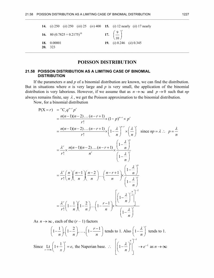
21.58 POISSON DISTRIBUTION AS A LIMITING CASE OF BINOMIAL DISTRIBUTION 1227 ________________________________________________________________________________________________________
14. (i) 250 (ii) 250 (iii) 25 (iv) 400 15. (i) 12 nearly (ii) 17 nearly
16. 80 (0.7825 + 0.2175)10 17. 49
10⎛ ⎞⎜ ⎟⎝ ⎠
18. 0.00001 19. (i) 0.246 (ii) 0.345 20. 323
________________________________________________________________________________________________________
POISSON DISTRIBUTION
21.58 POISSON DISTRIBUTION AS A LIMITING CASE OF BINOMIAL DISTRIBUTION
If the parameters n and p of a binomial distribution are known, we can find the distribution. But in situations where n is very large and p is very small, the application of the binomial distribution is very laborious. However, if we assume that as n →∞ and 0p → such that np always remains finite, say λ , we get the Poisson approximation to the binomial distribution.
Now, for a binomial distribution
P(X ) C( 1)( 2) . . . ( 1) (1 )
!( 1)( 2) . . . ( 1) 1 since
!
1( 1)( 2) . . . ( 1)
!1
1 2!
n n r rr
n r r
n r r
n
r
rr
r
r q pn n n n r p p
rn n n n r np p
r n n n
n n n n r nr n
n
n n nr n n n
λ λ λλ
λλ
λ
λ
−
−
−
= =− − − +
= × − ×
− − − + ⎛ ⎞ ⎛ ⎞= × − × = ∴ =⎜ ⎟ ⎜ ⎟⎝ ⎠ ⎝ ⎠
⎛ ⎞−⎜ ⎟− − − + ⎝ ⎠= × ×⎛ ⎞−⎜ ⎟⎝ ⎠
− −⎛ ⎞⎛ ⎞⎛ ⎞= ⎜ ⎟⎜ ⎟⎜ ⎟⎝ ⎠⎝ ⎠⎝ ⎠
11. . .
1
11 2 11 1 . . . 1
!1
n
r
n
r
r
n r nn
n
nrr n n n
n
λ
λ
λ
λ
λ
λλ
−−
⎛ ⎞−⎜ ⎟− +⎛ ⎞ ⎝ ⎠×⎜ ⎟⎝ ⎠ ⎛ ⎞−⎜ ⎟
⎝ ⎠
⎡ ⎤⎛ ⎞⎢ ⎥−⎜ ⎟⎢ ⎥⎝ ⎠−⎛ ⎞⎛ ⎞ ⎛ ⎞ ⎣ ⎦= − − − ×⎜ ⎟⎜ ⎟ ⎜ ⎟
⎝ ⎠⎝ ⎠ ⎝ ⎠ ⎛ ⎞−⎜ ⎟⎝ ⎠
As n →∞ , each of the (r – 1) factors
1 2 11 , 1 , . . . , 1 tends to 1. Also 1 tends to 1.rr
n n n nλ−⎛ ⎞ ⎛ ⎞ ⎛ ⎞ ⎛ ⎞− − − −⎜ ⎟ ⎜ ⎟ ⎜ ⎟ ⎜ ⎟
⎝ ⎠ ⎝ ⎠ ⎝ ⎠ ⎝ ⎠
Since 1Lt 1 , the Naperian base. 1 as nx
xe e n
x n
λ
λ λλ−
−
→
⎡ ⎤⎛ ⎞ ⎛ ⎞⎢ ⎥+ = ∴ − → →⎜ ⎟ ⎜ ⎟⎢ ⎥⎝ ⎠ ⎝ ⎠
⎣ ⎦∞
∞
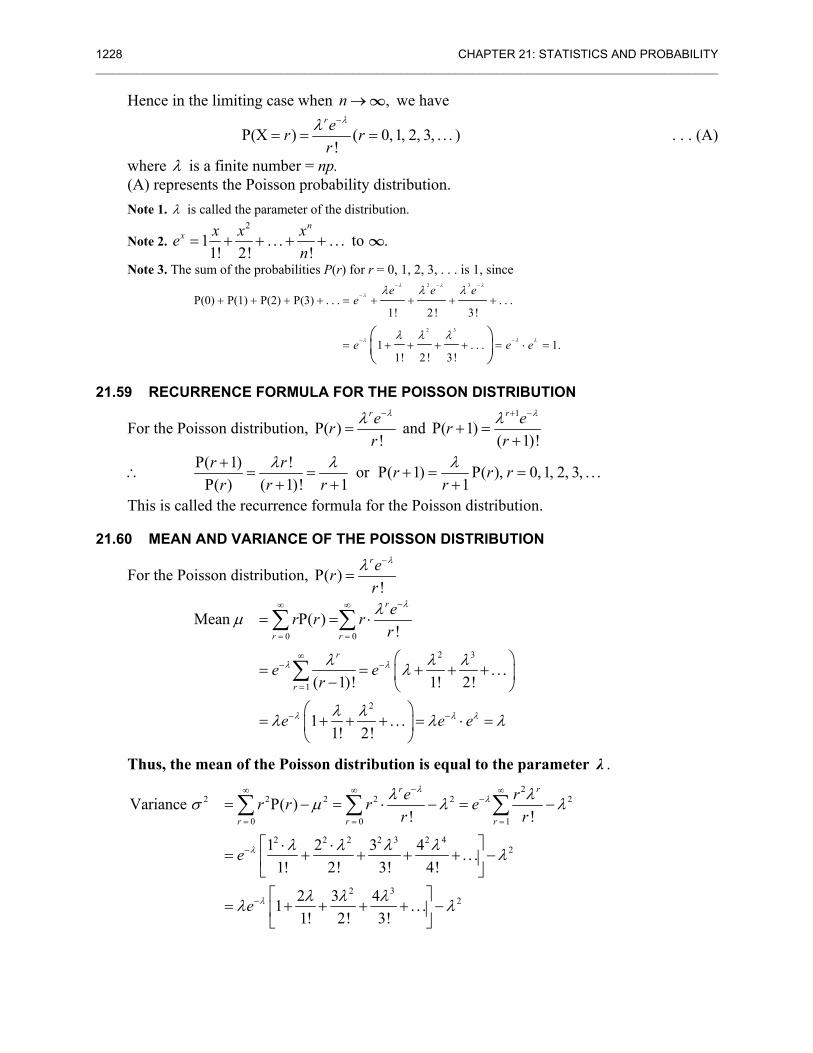
1228 CHAPTER 21: STATISTICS AND PROBABILITY ________________________________________________________________________________________________________
Hence in the limiting case when ,n →∞ we have
P(X ) ( 0,1, 2, 3, . . . )!
rer rr
λλ −
= = = . . . (A)
where λ is a finite number = np. (A) represents the Poisson probability distribution. Note 1. λ is called the parameter of the distribution.
Note 2. 2
1 . . . . . . to .1! 2! !
nx x x xe
n= + + + + ∞
Note 3. The sum of the probabilities P(r) for r = 0, 1, 2, 3, . . . is 1, since
2 3
2 3
P(0) P(1) P(2) P(3) . . . . . .1! 2! 3!
1 . . . 1.1! 2! 3!
e e ee
e e e
λ λ λ
λ
λ λ λ
λ λ λ
λ λ λ
− − −
−
− −
+ + + + = + + + +
= + + + + = ⋅ =⎛ ⎞⎜ ⎟⎝ ⎠
21.59 RECURRENCE FORMULA FOR THE POISSON DISTRIBUTION
For the Poisson distribution, P( )!
rerr
λλ −
= and 1
P( 1)( 1)!
r err
λλ + −
+ =+
∴ P( 1) ! or P( 1) P( ), 0,1, 2, 3, . . .P( ) ( 1)! 1 1r r r r r
r r r rλ λ λ+
= = + = =+ + +
This is called the recurrence formula for the Poisson distribution.
21.60 MEAN AND VARIANCE OF THE POISSON DISTRIBUTION
For the Poisson distribution, P( )!
rerr
λλ −
=
0 0
2 3
1
2
Mean P( )!
. . .( 1)! 1! 2!
1 . . .1! 2!
r
r r
r
r
er r rr
e er
e e e
λ
λ λ
λ λ λ
λμ
λ λ λλ
λ λλ λ λ
−∞ ∞
= =
∞− −
=
− −
= = ⋅
⎛ ⎞= = + + +⎜ ⎟− ⎝ ⎠
⎛ ⎞= + + + = ⋅ =⎜ ⎟
⎝ ⎠
∑ ∑
∑
Thus, the mean of the Poisson distribution is equal to the parameter λ . 2
2 2 2 2 2 2
0 0 1
2 2 2 2 3 2 42
2 32
Variance P( )! !
1 2 3 4 . . .1! 2! 3! 4!
2 3 41 . . .1! 2! 3!
r r
r r r
e rr r r er r
e
e
λλ
λ
λ
λ λσ μ λ λ
λ λ λ λ λ
λ λ λλ λ
−∞ ∞ ∞−
= = =
−
−
= − = ⋅ − = −
⎡ ⎤⋅ ⋅= + + + + −⎢ ⎥
⎣ ⎦⎡ ⎤
= + + + + −⎢ ⎥⎣ ⎦
∑ ∑ ∑
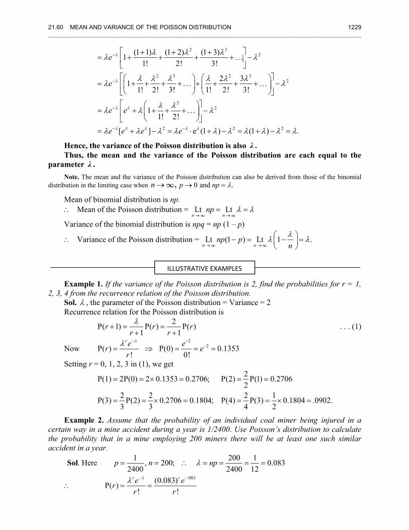
21.60 MEAN AND VARIANCE OF THE POISSON DISTRIBUTION 1229 ________________________________________________________________________________________________________
2 32
2 3 2 32
22
2 2 2
(1 1) (1 2) (1 3)1 . . .1! 2! 3!
2 31 . . . . . .1! 2! 3! 1! 2! 3!
1 . . .1! 2!
[ ] e (1 ) (1 ) .
e
e
e e
e e e e
λ
λ
λ λ
λ λ λ λ λ
λ λ λλ λ
λ λ λ λ λ λλ λ
λ λλ λ λ
λ λ λ λ λ λ λ λ λ λ
−
−
−
− −
⎡ ⎤+ + += + + + + −⎢ ⎥
⎣ ⎦⎡ ⎤⎛ ⎞ ⎛ ⎞
= + + + + + + + + −⎢ ⎥⎜ ⎟ ⎜ ⎟⎝ ⎠ ⎝ ⎠⎣ ⎦⎡ ⎤⎛ ⎞
= + + + + −⎢ ⎥⎜ ⎟⎝ ⎠⎣ ⎦
= + − = ⋅ + − = + − =
Hence, the variance of the Poisson distribution is also λ . Thus, the mean and the variance of the Poisson distribution are each equal to the
parameter λ . Note. The mean and the variance of the Poisson distribution can also be derived from those of the binomial
distribution in the limiting case when 0 and .p npn λ→ =→∞,
Mean of binomial distribution is np. ∴ Mean of the Poisson distribution = Lt Lt
n nnp λ λ
→ →= =
∞ ∞
Variance of the binomial distribution is npq = np (1 – p)
∴ Variance of the Poisson distribution = Lt (1 ) Lt 1 .n n
np pnλλ λ
→ →
⎛ ⎞− = − =⎜ ⎟⎝ ⎠∞ ∞
Example 1. If the variance of the Poisson distribution is 2, find the probabilities for r = 1, 2, 3, 4 from the recurrence relation of the Poisson distribution.
Sol. λ , the parameter of the Poisson distribution = Variance = 2 Recurrence relation for the Poisson distribution is
2P( 1) P( ) P( )1 1
r r rr rλ
+ = =+ +
. . . (1)
Now 2
2P( ) P(0) 0.1353! 0!
re er er
λλ − −−= ⇒ = = =
Setting r = 0, 1, 2, 3 in (1), we get
2P(1) 2P(0) 2 0.1353 0.2706; P(2) P(1) 0.27062
2 2 2 1P(3) P(2) 0.2706 0.1804; P(4) P(3) 0.1804 .0902.3 3 4 2
= = × = = =
= = × = = = × =
Example 2. Assume that the probability of an individual coal miner being injured in a certain way in a mine accident during a year is 1/2400. Use Poisson’s distribution to calculate the probability that in a mine employing 200 miners there will be at least one such similar accident in a year.
.083
1 200 1. Here , 200; 0.0832400 2400 12
(0.083)P( )! !
r r
p n np
e err r
λ
λ
λ − −
= = ∴ = = = =
∴ = =
Sol
ILLUSTRATIVE EXAMPLES
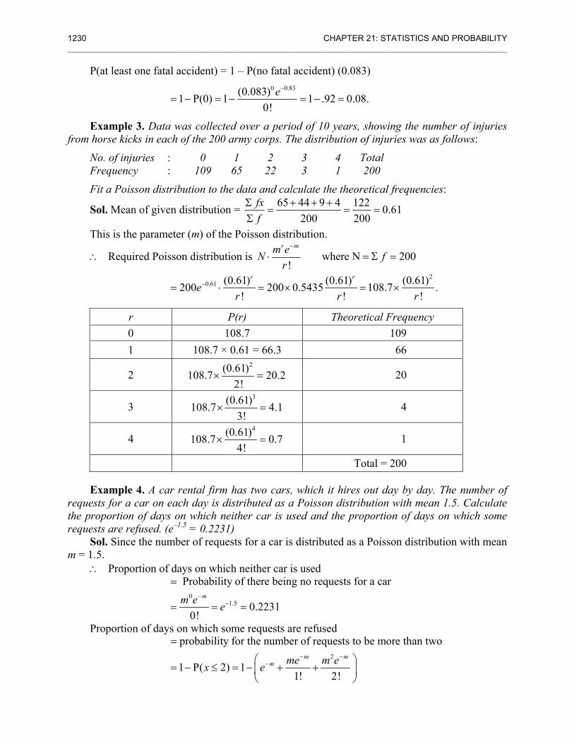
1230 CHAPTER 21: STATISTICS AND PROBABILITY ________________________________________________________________________________________________________
P(at least one fatal accident) = 1 – P(no fatal accident) (0.083)
0 0.83(0.083)1 P(0) 1 1 .92 0.08.
0!e−
= − = − = − =
Example 3. Data was collected over a period of 10 years, showing the number of injuries from horse kicks in each of the 200 army corps. The distribution of injuries was as follows:
No. of injuries : 0 1 2 3 4 Total Frequency : 109 65 22 3 1 200
Fit a Poisson distribution to the data and calculate the theoretical frequencies:
Sol. Mean of given distribution = 65 44 9 4 122 0.61200 200
fxf
Σ + + += = =
Σ
This is the parameter (m) of the Poisson distribution.
∴ Required Poisson distribution is !
r mm eNr
−
⋅ where N 200f= Σ =
2
0.61 (0.61) (0.61) (0.61)200 200 0.5435 108.7 .! ! !
r r
er r r
−= ⋅ = × = ×
r P(r) Theoretical Frequency 0 108.7 109 1 108.7 × 0.61 = 66.3 66
2 2(0.61)108.7 20.2
2!× = 20
3 3(0.61)108.7 4.1
3!× = 4
4 4(0.61)108.7 0.7
4!× = 1
Total = 200
Example 4. A car rental firm has two cars, which it hires out day by day. The number of requests for a car on each day is distributed as a Poisson distribution with mean 1.5. Calculate the proportion of days on which neither car is used and the proportion of days on which some requests are refused. (e–1.5 = 0.2231)
Sol. Since the number of requests for a car is distributed as a Poisson distribution with mean m = 1.5.
∴ Proportion of days on which neither car is used
01.5
Probability of there being no requests for a car
0.22310!
mm e e−
−
=
= = =
Proportion of days on which some requests are refused
2
probability for the number of requests to be more than two
1 P( 2) 11! 2!
m mm me m ex e
− −−
=
⎛ ⎞= − ≤ = − + +⎜ ⎟
⎝ ⎠
21.60 MEAN AND VARIANCE OF THE POISSON DISTRIBUTION 1231 ________________________________________________________________________________________________________
21.5 (1.5)1 1 1.5 1 0.2231 (1 1.5 1.125)
21 0.2231 3.625 1 0.8087375 0.1912625.
e− ⎛ ⎞= − + + = − + +⎜ ⎟
⎝ ⎠= − × = − =
Example 5. Six coins are tossed 6400 times. Using the Poisson distribution, determine the approximate probability of getting six heads x times.
Sol. Probability of getting one head with one coin = 12 .
∴ The probability of getting six heads with six coins = 61 1
2 64⎛ ⎞ =⎜ ⎟⎝ ⎠
∴ Average number of six heads with six coins in 6400 throws = np = 6400 × 164
= 100
∴ The mean of the Poisson distribution = 100.
Approximate probability of getting six heads x times when the distribution is Poisson
100(100) .
! (100)!
x m xm e ex
− −⋅= =
1. Fit a Poisson distribution to the following:
x : 0 1 2 3 4 f : 192 100 24 3 1
2. If the probability of a bad reaction from a certain injection is 0.001, determine the chance that out of 2000 individuals more than two will get a bad reaction.
3. If X is a Poisson variate such that P(X = 2) = 9P(X = 4) + 90P(X = 6), find the standard deviation.
4. If a random variable has a Poisson distribution such that P(1) = P(2), find
(i) mean of the distribution (ii) P(4)
5. Suppose that X has a Poisson distribution. If P(X = 2) = 23 P(X = 1) find, (i) P(X = 0) (ii) P(X = 3).
6. A certain screw-making machine produces on average 2 defective screws out of 100, and packs them in boxes of 500. Find the probability that a box contains 15 defective screws.
7. The incidence of occupational disease in an industry is such that the workmen have a 10% chance of suffering from it. What is the probability that in a group of 7, five or more will suffer from it?
8. Fit a Poisson distribution to the following and calculate theoretical frequencies:
x : 0 1 2 3 4 f : 122 60 15 2 1
9. Fit a Poisson distribution to the following data given the number of yeast cells per square for 400 squares:
No. of cells per sq. : 0 1 2 3 4 5 6 7 8 9 10 No. of squares : 103 143 98 42 8 4 2 0 0 0 0
10. Show that in a Poisson distribution with unit mean, mean deviation about mean is 2e
⎛ ⎞⎜ ⎟⎝ ⎠
times the
TEST YOUR KNOWLEDGE
standard deviation.
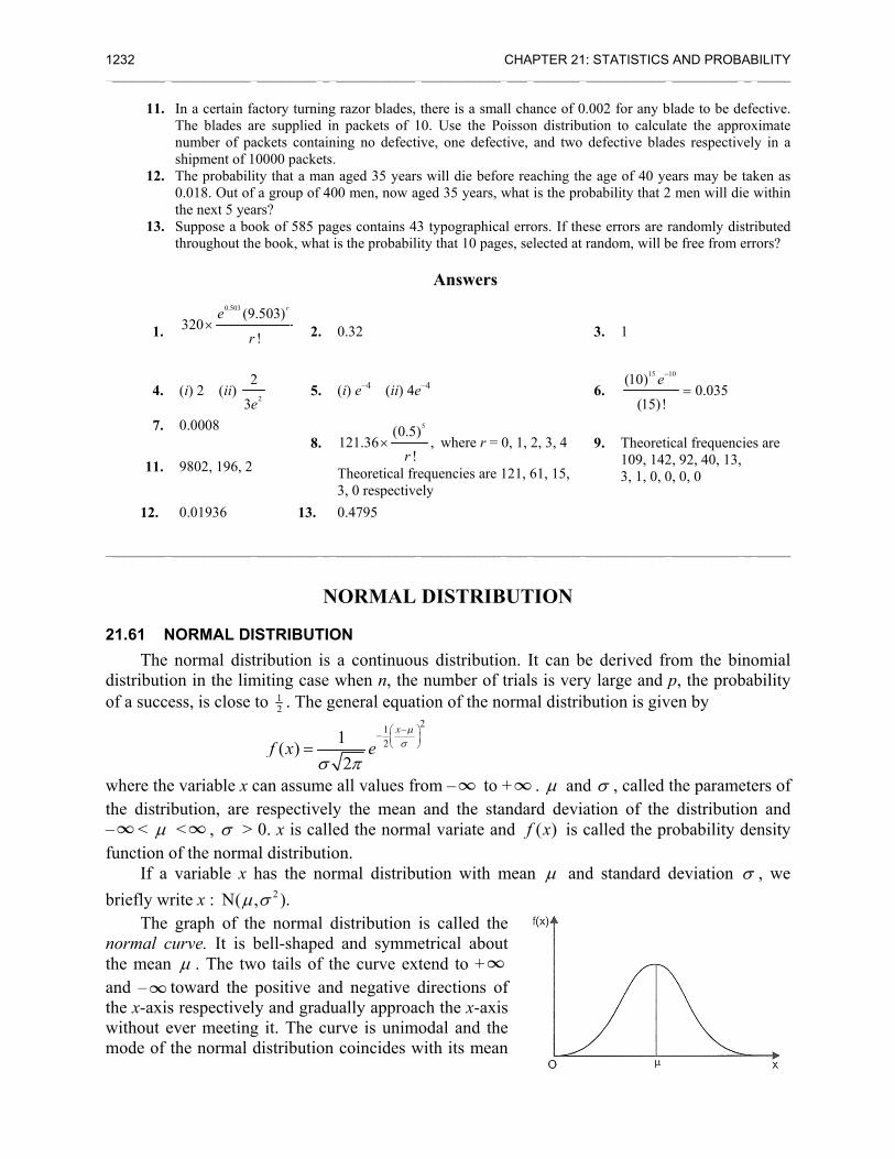
1232 __________
11.
12.
13.
1.
4.
7.
11.
12. __________
21.61 NThe
distributiof a succ
where thethe distri–∞ < μfunction
If a briefly w
Thenormal cthe meanand –∞the x-axiwithout emode of
______________
In a certain fThe blades anumber of pshipment of 1The probabil0.018. Out ofthe next 5 yeaSuppose a bothroughout th
0.503 (9320
e
r×
(i) 2 (ii) 2
30.0008
9802, 196, 2
0.01936
______________
NORMAL D normal dision in the limess, is close
e variable x ibution, are
μ <∞ , σ >of the normavariable x
write x : N(μ graph of thcurve. It is n μ . The twtoward the s respectivelever meetingthe normal
_____________
factory turningare supplied inackets contain10000 packets.ity that a man f a group of 40ars? ook of 585 paghe book, what i
9.503)
!
r
r 2.
2
2
e 5.
8. 2
13.
_____________
N
ISTRIBUTIOtribution is miting case wto 1
2 . The g
( )f xσ
=
can assume respectively
> 0. x is calleal distributiohas the nor
2, ).μ σ he normal dbell-shaped
wo tails of thpositive an
ly and gradug it. The cudistribution
______________
g razor blades, n packets of 1ning no defecti. aged 35 years
00 men, now ag
ges contains 43is the probabili
0.32
(i) e–4 (ii) 4e
(0.5)121.36
!r×
Theoretical fre3, 0 respective0.4795
______________
NORMAL
ON a continuouwhen n, the
general equat121
2
x
eμ
σ
π
−⎛ ⎞− ⎜⎝ ⎠
all values fry the mean ed the normon. rmal distribu
distribution and symme
he curve extd negative dually approaurve is unim
coincides w
______________
there is a sma10. Use the Poive, one defec
s will die befoged 35 years, w
3 typographicaity that 10 page
Answers
e–4
5), where r = 0
equencies are 1ely
______________
DISTRIB
us distributionumber of
tion of the no2⎞⎟⎠
rom –∞ to +and the sta
al variate an
ution with m
is called theetrical aboutend to +∞directions och the x-axisodal and the
with its mean
CHAPTER 21_____________
all chance of 0oisson distributive, and two
re reaching thewhat is the pro
al errors. If thees, selected at r
0, 1, 2, 3, 4
121, 61, 15,
_____________
BUTION
on. It can betrials is veryormal distrib
+∞ . μ andandard deviand ( )f x is c
mean μ and
e ut
∞ f s e n
: STATISTICS ______________
.002 for any bution to calculdefective blad
e age of 40 yeobability that 2
ese errors are rrandom, will b
3. 1
6. 15 1(10)
(15)!
e−
9. Theoreti109, 1423, 1, 0, 0
______________
e derived fry large and pbution is giv
d σ , called tation of the called the pr
d standard d
AND PROBAB______________
lade to be defeate the approx
des respectivel
ears may be tak2 men will die w
randomly distrbe free from err
10
0.035=
ical frequencie2, 92, 40, 13, 0, 0, 0
______________
rom the binop, the proba
ven by
the parametedistribution
robability de
deviation σ
BILITY ______
fective. ximate ly in a
ken as within
ributed rors?
s are
______
omial ability
ers of n and ensity
σ , we
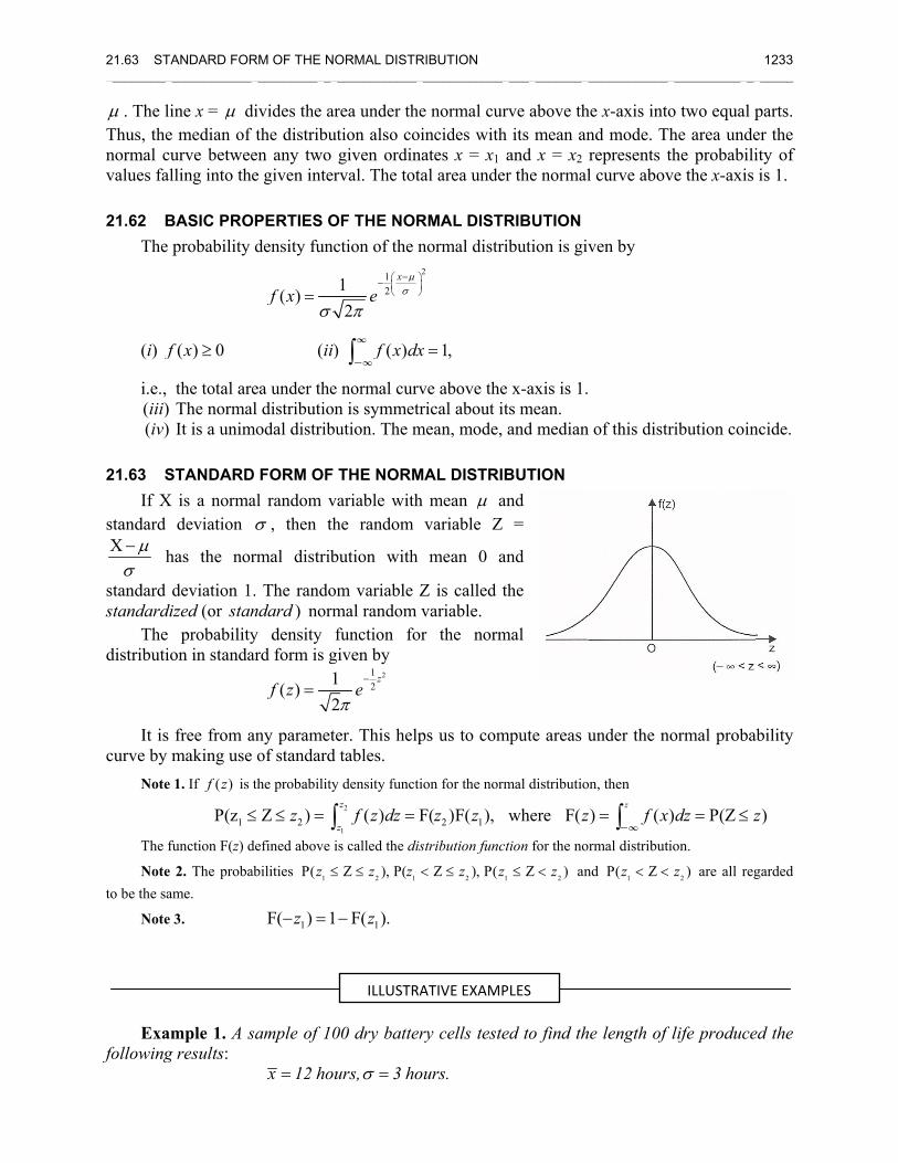
21.63 ST__________
μ . The lThus, thenormal cvalues fa
21.62 BThe
(i) f
i.e., (iii) (iv)
21.63 SIf X
standard X μσ− h
standard standard
Thedistributi
It iscurve by
Note
The f
Noteto be the sa
Note
Exafollowing
TANDARD FOR______________
line x = μ de median of curve betweealling into the
BASIC PRO probability
( ) 0f x ≥
the total are) The norma) It is a unim
STANDARDX is a norma
deviation
has the nor
deviation 1dized (or stan probabilityion in standa
s free from amaking use
e 1. If ( )f z is
1P(z ≤
function F(z) d
e 2. The probaame.
e 3.
ample 1. A sg results:
RM OF THE NO_____________
divides the arthe distribu
en any two e given inter
OPERTIES Odensity func
( )f xσ
=
(ii)
ea under theal distributionmodal distribu
D FORM OF al random vσ , then th
rmal distrib
. The rando)ndard norm
y density fard form is g
1( )2
f z =
any paramete of standard the probability
2Z )z≤ ≤ = ∫defined above i
abilities 1P(z ≤
1F( ) 1z− =
sample of 10
x 12 hou=
ORMAL DISTR______________
rea under theution also co
given ordinrval. The tot
OF THE NORction of the n
121
2
x
eμ
σ
π
−⎛ ⎞− ⎜⎝ ⎠
) ( )f x dx∫∞
∞−
e normal curvn is symmetrution. The m
THE NORMvariable withhe random
bution with
m variable Zmal random function fo
given by 21
212
ze
π−
er. This helptables.
y density functi2
1
( ) Fz
zf z dz =
is called the dis
2 1Z ), P(z z≤ ≤
1F( ).z−
00 dry batter
urs, 3 hoσ =
ILLUSTRA
RIBUTION______________
e normal curincides with
nates x = x1tal area unde
RMAL DISTnormal distr2⎞⎟⎠
1,x =
ve above therical about it
mean, mode,
MAL DISTRIh mean μ a
variable Z
mean 0 a
Z is called tvariable.
or the norm
ps us to com
ion for the norm
2 1F( )F( ),z z
stribution func
2Z ), P(z z< ≤
ry cells teste
ours.
ATIVE EXAMP
_____________
rve above thh its mean anand x = x2
er the normal
RIBUTION ibution is giv
e x-axis is 1.ts mean. and median
BUTION and
=
and
the
mal
mpute areas u
mal distributio
where F(z
ction for the no
1 2Z )z z≤ < an
ed to find th
PLES
______________
he x-axis intond mode. Threpresents thl curve abov
ven by
n of this distr
under the no
on, then
) ( )z
z f x= ∫ ∞−
ormal distributi
nd 1P( Zz < <
he length of
______________
o two equal phe area undehe probabili
ve the x-axis
ribution coin
ormal proba
) P(Zdz z= ≤
ion.
2 )z are all reg
life produce
1233 ______
parts. er the ity of is 1.
ncide.
ability
)z
garded
ed the
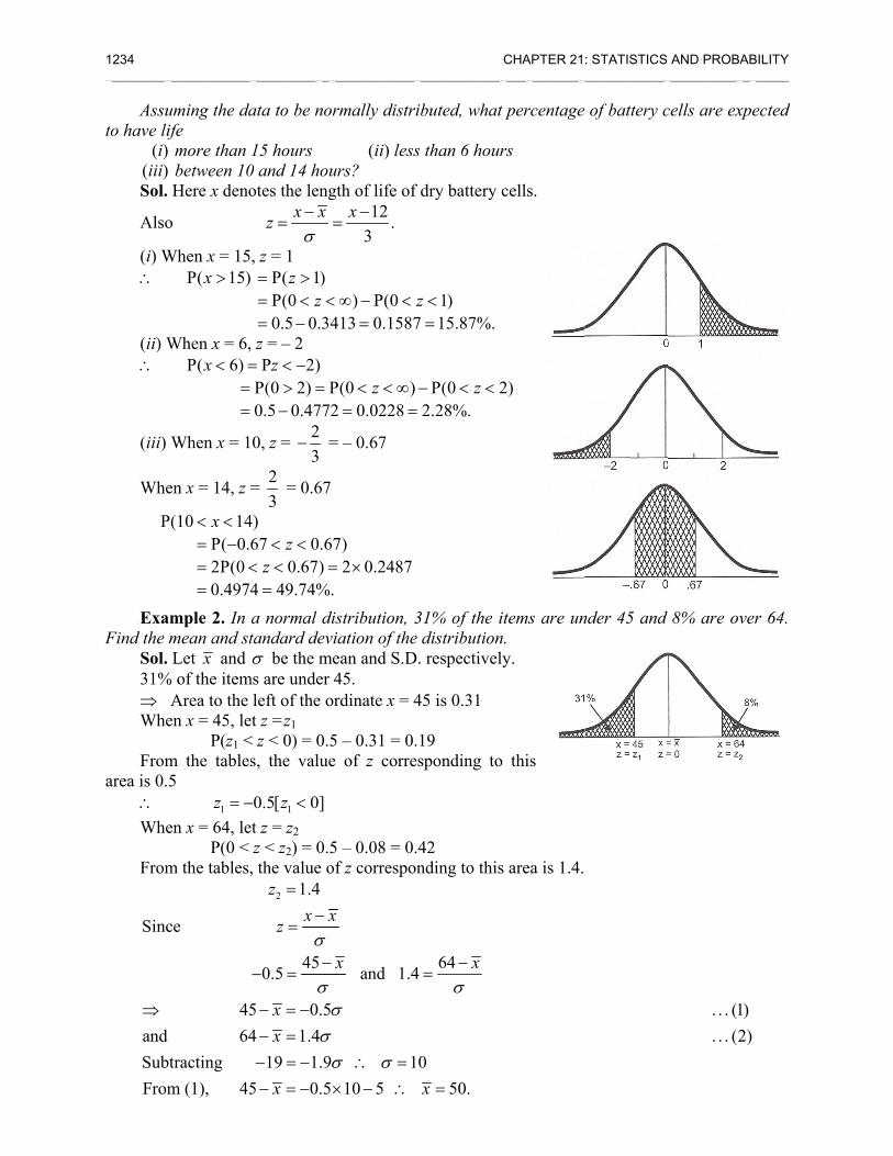
1234 __________
Assuto have li
(i) (iii)Sol.
Also
(i) W∴
(ii) W∴
(iii)
Whe
P
ExaFind the
Sol.31%⇒ Whe From
area is 0.∴ Whe From
Sinc
andSubFrom
⇒
______________
uming the daife ) more than ) between 10 Here x deno
o
When x = 15P( 15)x >
When x = 6,P( 6)x < =
==
When x = 1
en x = 14, z =
P(10 14P( 0.2P(00.4974
x< <= −= <=
ample 2. In mean and st Let x and
% of the itemArea to the
en x = 45, leP(z1 <
m the tables5
1z = −en x = 64, le
P(0 < m the tables,
ce
45d 64btractingm (1), 45
_____________
ata to be nor
15 hours 0 and 14 houotes the leng
x xzσ−
= =
, z = 1 P( 1)P(00.5 0.34
zz
= >= < <= −
, z = – 2 P 2)
P(0 2) P0.5 0.4772
z= < −> =−
0, z = 23
− =
= 23
= 0.67
4)67 0.67
0.67)4 49.74%.
zz< <
< < ==
a normal ditandard deviσ be the me
ms are under 4left of the or
et z =z1 < z < 0) = 0.5s, the value
10.5[ 0]z− < et z = z2
z < z2) = 0.5, the value o
2 1.4
450.5
5 0.54 1.4
19 1.95 0.5
zx xz
xx
x
σ
σσ
σσ
=−
=
−− =
− = −− =− = −− = − ×
______________
rmally distri
(ii) lessurs? gth of life of
12 .3
x −=
) P(0413 0.1587
z< ∞ − <=
P(0 )2 0.0228
z< < ∞= =
= – 0.67
7)2 0.2487= ×
istribution, 3iation of the ean and S.D45. rdinate x = 4
5 – 0.31 = 0.e of z corre
5 – 0.08 = 0.f z correspon
and 1.4
110 5
x
x
σ
σ σ∴ =× − ∴
______________
ibuted, what
s than 6 hour
dry battery
1)7 15.87%.z <=
P(0 22.28%.
z− < <
31% of the idistribution
. respectivel
45 is 0.31
19 sponding to
42 nding to this
644
050.
x
x
σ−
=
=
CHAPTER 21_____________
t percentage
rs
cells.
2)
items are unn. ly.
o this
s area is 1.4.
: STATISTICS ______________
of battery c
nder 45 and
AND PROBAB______________
cells are exp
8% are ove
. . . (1)
. . . (2)
BILITY ______
ected
er 64.
21.64 POPULATION OR UNIVERSE 1235 ________________________________________________________________________________________________________
1. The mean height of 500 students in a certain college is 151 cm and the standard deviation is 15 cm. Assuming the heights are normally distributed, how many students have heights between 120 and 155 cm?
2. An aptitude test for selecting officers in a bank is conducted on 1000 candidates. The average score is 42 and the standard deviation of score is 24. Assuming normal distribution for the scores, find
(i) The number of candidates whose scores exceed 60 (ii) The number of candidates whose scores lie between 30 and 60.
3. In a normal distribution, 7% of the items are under 35 and 89% are under 63. What are the mean and standard deviation of the distribution?
4. Let X denote the number of scores on a test. If X is normally distributed with mean 100 and standard deviation 15, find the probability that X does not exceed 130.
5. It is known from past experience that the number of telephone calls made daily in a certain community between 3 P.M. and 4 P.M. have a mean of 352 and a standard deviation of 31. What percentage of the time will there be more than 400 telephone calls made in this community between 3 P.M. and 4 P.M.?
6. Students of a class were given a mechanical aptitude test. Their grades were found to be normally distributed with mean 60 and standard deviation 5. What percent of students scored
(i) more than 60 grades? (ii) less than 56 grades? (iii) between 45 and 65 grades?
7. In an examination taken by 500 candidates, the average and the standard deviation of grades obtained (normally distributed) are 40% and 10%. Find approximately:
(i) How many will pass, if 50% is fixed as a minimum? (ii) What should be the minimum if 350 candidates are to pass? (iii) How many have scored above 60%?
Answers 1. 300 2. (i) 252 (ii) 533 3. 50.3, 10.33x σ= =
4. 0.9772 5. 6.06% 6. (i) 50% (ii) 21.2% (iii) 84%
7. (i) 79 (ii) 35% (iii) 11 ________________________________________________________________________________________________________
SAMPLING AND TESTS OF SIGNIFICANCE
21.64 POPULATION OR UNIVERSE An aggregate of objects (animate or inanimate) under study is called population or
universe. It is thus a collection of individuals or of their attributes (qualities) or of results of operations that can be numerically specified.
A universe containing a finite number of individuals or members is called a finite inverse: for example, the universe of the weights of students in a particular class.
A universe with an infinite number of members is known as an infinite universe: for example, the universe of pressures at various points in the atmosphere.
In some cases, we may even be ignorant whether or not a particular universe is infinite, e.g., the universe of stars.
TEST YOUR KNOWLEDGE
1236 CHAPTER 21: STATISTICS AND PROBABILITY ________________________________________________________________________________________________________
The universe of concrete objects is an existent universe. The collection of all possible ways in which a specified event can happen is called a hypothetical universe. The universe of heads and tails obtained by tossing a coin an infinite number of times (provided that it does not wear out) is a hypothetical one.
21.65 SAMPLING The statistician is often confronted with the problem of discussing a universe of which he
cannot examine every member, i.e., of which complete enumeration is impracticle. For example, if we want to have an idea of the average per capita income of the United States, enumeration of every earning individual in the country is a very difficult task. Naturally, the question arises: What can be said about a universe of which we can examine only a limited number of members? This question is the origin of the Theory of Sampling.
A finite sub-set of a universe is called a sample. A sample is thus a small portion of the universe. The number of individuals in a sample is called the sample size. The process of selecting a sample from a universe is called sampling.
The theory of sampling is a study of the relationship existing between a population and samples drawn from the population. The fundamental object of sampling is to get as much information as possible about the whole universe by examining only a part of it. An attempt is thus made through sampling to give the maximum information about the parent universe with the minimum effort.
Sampling is quite often used in our day-to-day practical life. For example, in a store we assess the quality of lettuce, apples, or any other commodity by taking only a handful of it from the bag and then decide whether to purchase it or not. A chef normally tastes cooked products to find if they have been properly cooked and contain the proper quantity of salt or sugar, by taking a spoonful of it.
21.66 PARAMETERS OF STATISTICS The statistical constants of the population such as mean, the variance, etc. are known as the
parameters. The statistical concepts of the sample from the members of the sample to estimate the parameters of the population from which the sample has been drawn are known as statistics.
Population mean and variance are denoted by μ and 2σ , while those of the sample are given by 2 and .x s
21.67 STANDARD ERROR (S.E.) The standard deviation of the sampling distribution of a statistic is known as the standard
error (S.E.). It plays an important role in the theory of large samples and it forms a basis of the testing of
hypotheses. If t is any statistic, for a large sample
E( )S.E.( )t tz
t−
= is normally distributed with mean 0 and variance 1.
For a large sample, the standard errors of some of the well-known statistics are listed below:
n sample size p population proportion 2σ population variance Q = 1 – p 2s sample variance 1 2,n n sizes of two independent random samples
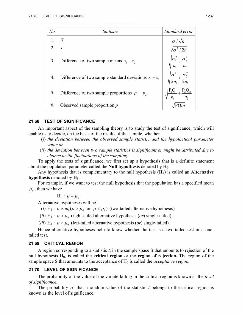
21.70 LEVEL OF SIGNIFICANCE 1237 ________________________________________________________________________________________________________
No. Statistic Standard error
1.
2.
3.
4.
5.
6.
x
s
Difference of two sample means 1 2x x−
Difference of two sample standard deviations 1 2s s−
Difference of two sample proportions 1 2p p−
Observed sample proportion p
2
2 21 2
1 2
2 21 2
1 2
1 1 2 2
1 2
/
/ 2
2 2
P Q P Q
PQ/
n
n
n n
n n
n n
n
σ
σ
σ σ
σ σ
+
+
+
21.68 TEST OF SIGNIFICANCE An important aspect of the sampling theory is to study the test of significance, which will
enable us to decide, on the basis of the results of the sample, whether (i) the deviation between the observed sample statistic and the hypothetical parameter
value or (ii) the deviation between two sample statistics is significant or might be attributed due to
chance or the fluctuations of the sampling. To apply the tests of significance, we first set up a hypothesis that is a definite statement
about the population parameter called the Null hypothesis denoted by H0. Any hypothesis that is complementary to the null hypothesis (H0) is called an Alternative
hypothesis denoted by H1. For example, if we want to test the null hypothesis that the population has a specified mean
0μ , then we have H0 : 0μ μ= Alternative hypotheses will be (i) H1 : 0 0 0( or )mμ μ μ μ μ≠ > < (two-tailed alternative hypothesis). (ii) H1 : 0μ μ> (right-tailed alternative hypothesis (or) single-tailed). (iii) H1 : 0μ μ< (left-tailed alternative hypothesis (or) single-tailed). Hence alternative hypotheses help to know whether the test is a two-tailed test or a one-
tailed test.
21.69 CRITICAL REGION A region corresponding to a statistic t, in the sample space S that amounts to rejection of the
null hypothesis H0, is called the critical region or the region of rejection. The region of the sample space S that amounts to the acceptance of H0 is called the acceptance region.
21.70 LEVEL OF SIGNIFICANCE The probability of the value of the variate falling in the critical region is known as the level
of significance. The probability α that a random value of the statistic t belongs to the critical region is
known as the level of significance.
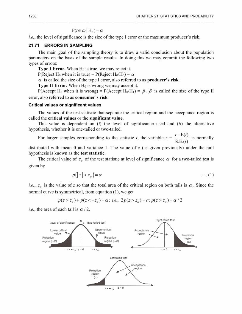
1238 __________
i.e., the le
21.71 EThe
parametetypes of e
TypP(Rα iTypP(A
error, alsCritical v
Thecalled the
Thishypothes
For
distributehypothes
Thegiven by
i.e., zα inormal c
i.e., the a
______________
evel of signi
ERRORS IN main goal
ers on the baerrors:
pe I Error. WReject H0 whe
s called the pe II Error.
Accept H0 who referred tovalues or si
values of the critical vas value is dsis, whether i
larger samp
ed with measis is known critical valu
s the value ourve is symm
(p z >
area of each t
_____________
P( | Ht ω∈ificance is th
N SAMPLINGof the sampasis of the s
When H0 is ten it is true) size of the tyWhen H0 is
hen it is wroo as consumignificant va
he test statisalues or the sdependent oit is one-tail
ples corresp
an 0 and vaas the test s
ue of zα of t
(p z zα>
of z so that metrical, fro
) (z p zα> + <
tail is / 2.α
______________
0H ) α= he size of the
G pling theory sample resul
true, we may= P(Reject H
ype I error, awrong we m
ong) = P(Acmer’s risk.
alues
stic that sepasignificant von (i) the led or two-ta
ponding to th
ariance 1. Tstatistic. the test stati
)α α=
the total arem equation
) ;z iα α− =
______________
e type I error
is to draw lts. In doing
y reject it. H0/H0) = αalso referredmay accept itccept H0/H1)
arate the critvalue. level of sigailed.
he statistic
The value of
stic at level
ea of the crit(1), we get
. ., 2 (i e p z z>
CHAPTER 21_____________
r or the maxi
a valid concthis we ma
d to as produt. = .β β is
tical region
gnificance u
t, the variab
f z (as given
of significan
tical region
) ; (z a p zα =
: STATISTICS ______________
imum produ
clusion abouay commit th
ucer’s risk.
called the s
and the acc
used and (ii
ble z = ES.Et −
n previously
nce α for a
on both tails
) / 2zα α> =
AND PROBAB______________
ucer’s risk.
ut the populhe following
ize of the ty
eptance regi
i) the altern
E( )E.( )
tt
is norm
y) under the
two-tailed t
.
s is α . Sinc
2
BILITY ______
lation g two
ype II
ion is
native
mally
e null
test is
. . (1)
ce the
21.72 TESTING OF SIGNIFICANCE FOR A SINGLE PROPORTION 1239 ________________________________________________________________________________________________________
The critical value zα is that value such that the area to the right of zα is / 2α and the area to the left of – zα is / 2.α
In the case of the one-tailed test
( )p z zα> = α if it is right tailed; p(z < – zα ) = α if it is left tailed.
The critical value of z for a single-tailed test (right or left) at the level of significance α is the same as the critical value of z for a two-tailed test at the level of significance 2 .α
Using the equation and the normal tables, the critical value of z at a different level of significance (α ) for both single-tailed and two-tailed tests are calculated and listed below. The equations are
( ) ; ( ) ; ( )p z z p z z p z zα α αα α α> = > = < − =
Level of significance 1% (0.01) 5% (0.05) 10% (0.1)
Two-tailed test 2.58zα = 1.966z = 0.645z =
Right-tailed 2.33zα = 1.645zα = 1.28zα =
Left-tailed 2.33zα = − 1.645zα = − 1.28zα = −
Note. The following steps may be adopted to test statistical hypotheses: Step 1: Null hypothesis. Set up H0 in clear terms. Step 2: Alternative hypothesis. Set up H1 so that we can decide whether to use the one-
tailed test or the two-tailed test. Step 3: Level of significance. Select the appropriate level of significance in advance
depending on the reliability of the estimates.
Step 4: Test statistic. Compute the test statistic z = E( )S.E.( )t t
t− under the null hypothesis.
Step 5: Conclusion. Compare the computed value of z with the critical value zα at the level of significance (α ).
If ,z zα> we reject H0 and conclude that there is significant difference. If ,z zα< we accept H0 and conclude that there is no significant difference.
TEST OF SIGNIFICANCE FOR LARGE SAMPLES
If the sample size n > 30, the sample is taken as a large sample. For such a sample we apply a normal test, as Binomial, Poisson, chi-square, etc. are closely approximated by normal distributions assuming the population as normal.
Under a large sample test, the following are the important tests of significance. 1. Testing of significance for a single proportion. 2. Testing of significance for a difference of proportions. 3. Testing of significance for a single mean. 4. Testing of significance for a difference of means.
21.72 TESTING OF SIGNIFICANCE FOR A SINGLE PROPORTION This test is used to find the significant difference between the proportion of the sample and
the population.
1240 CHAPTER 21: STATISTICS AND PROBABILITY ________________________________________________________________________________________________________
Let X be the number of successes in n independent trials with constant probability P of success for each trial.
E(X) = nP; V(X) = nPQ; Q = 1 – P = Probability of failure. Let p = X/n called the observed proportion of success.
2
1E( ) E(X/ ) E( ) ; E( )
1 1(PQ)V( ) V(X/ ) (X) PQ/
PQ E( )S.E.( ) ; N(0,1)SE( ) PQ/
npp n x p p pn n
p n v nn np p p pp z
n p n
= = = = =
= = = =
− −= = = ∼
This z is called the test statistic that is used to test the significant difference of sample and population proportion.
Note 1. The probable limit for the observed proportion of successes is p ± PQ/ ,z nα where zα is the significant value at level of significance .α
Note 2. If p is not known, the limits for the proportion in the population are p ± / ,z pq nα q = 1 – p. Note 3. If α is not given, we can take safely 3σ limits.
Hence, the confidence limits for the observed proportion p are p ± 3 PQ
.n
The confidence limits for the population proportion p are p ± .pq
n
Example 1. A coin was tossed 400 times and returned heads 216 times. Test the hypothesis that the coin is unbiased.
Sol. H0: The coin is unbiased, i.e., P = 0.5. H1: The coin is not unbiased (biased), i.e., P ≠ 0.5 Here n = 400; X = No. of success = 216
p = proportion of success in the sample X 216 0.54400n
= =
population proportion = 0.5 = P; Q = 1 – P = 1 – 0.5 = 0.5
under H0, test statistic z = PPQ/p
n−
0.54 0.5 1.60.5 0.5
400
z −= =
×
we use the two-tailed test. Conclusion. Since z = 1.6 < 1.96
I.e., ,z z zα α< is the significant value of z at 5% level of significance. I.e., the coin is unbiased in P = 0.5.
ILLUSTRATIVE EXAMPLES
21.72 TESTING OF SIGNIFICANCE FOR A SINGLE PROPORTION 1241 ________________________________________________________________________________________________________
Example 2. A certain cubical die was thrown 9000 times and a 5 or a 6 was obtained 3240 times. On the assumption of unbiased throwing, do the data indicate an unbiased die?
Sol. Here n = 9000 P = probability of success (i.e., getting a 5 or a 6 in the throw of the die) P = 2/6 = 1/3, Q = 1 – 1/3 = 2/3
X 3240 0.369000
pn
= = =
H0 : is unbiased, i.e., P = 1/3 H1 : P ≠ 1/3 (two-tailed test)
The test statistic
P 0.36 0.33 0.03496PQ 1 2 1
3 3 90000.03496 1.96
pz
nz
− −= = =
× ×
= <
Conclusion. Accept the hypothesis As ,z z zα α< is the tabulated value of z at 5% level of significance. ∵ H0 is accepted, we conclude that the die is unbiased.
Example 3. A manufacturer claims that only 4% of his products supplied are defective. A random sample of 600 products contained 36 defectives. Test the claim of the manufacturer.
Sol. (i) P = observed proportion of success.
I.e., P = proportion of defectives in the sample = 36600
= 0.06
p = proportion of defectives in the population = 0.04 H0 : p = 0.04 is true.
I.e., the claim of the manufacturer is accepted. H1 : (i) P ≠ 0.04 (two-tailed test) (ii) If we want to reject, only if p > 0.04 then (right tailed).
Under H0, P 0.06 0.04 2.5.PQ/ 0.04 0.96
600
pzn
− −= = =
×
Conclusion. Since z = 2.5 > 1.96, we reject the hypothesis H0 at 5% level of significance two tailed.
If H1 is taken as p > 0.04, we apply the right-tailed test. z = 2.5 > 1.645 ( )zα so we reject the null hypothesis here also.
In both cases, the manufacturer’s claim is not acceptable.
Example 4. A machine is producing bolts of which a certain fraction is defective. A random sample of 400 is taken from a large batch and is found to contain 30 defective bolts. Does this indicate that the proportion of defectives is larger than that claimed by the manufacturer who claims that only 5% of his products are defective? Find the 95% confidence limits of the proportion of defective bolts in the batch.
1242 CHAPTER 21: STATISTICS AND PROBABILITY ________________________________________________________________________________________________________
Sol. Null hypothesis. H0 : The manufacturer’s claim is accepted, i.e., P = 5100
= 0.05
Q = 1 – P = 1 – 0.05 = 0.95
Alternative hypothesis. p > 0.05 (right-tailed test).
p = observed proportion of sample = 30400
= 0.075
Under H0, the test statistic P 0.075 0.05 2.2941.PQ/ 0.05 0.95
400
pz zn
− −= ∴ = =
×
Conclusion. The tabulated value of z at 5% level of significance for the right-tailed test is
zα = 1.645. Since z = 2.2941 > 1.645,
H0 is rejected at 5% level of significance, i.e., the proportion of defective bolts is larger than the manufacturer claims.
To find 95% confidence limits of the proportion, it is given by p ± PQ/z nα
0.05 0.950.05 1.96 0.05 0.02135 0.07136, 0.02865400×
± = ± =
Hence 95% confidence limits for the proportion of defective bolts are (0.07136, 0.02865).
Example 5. A bag contains defective articles, the exact number of which is not known. A sample of 100 from the bag gives 10 defective articles. Find the limits for the proportion of defective articles in the bag.
Sol. Here p = proportion of defective articles = 10100
= 0.1; q = 1 – p = 1– 0.1 = 0.9.
Since the confidence limit is not given, we assume it is 95%. ∴ level of significance is 5% zα = 1.96. Also the proportion of population P is not given. To get the confidence limit, we use P,
which is given by P ± / 0.1pq n = ±0.1 0.91.96
100× = 0.1 ± 0.0588 = 0.1588, 0.0412.
Hence, the 95% confidence limits for the defective articles in the bag are (0.1588, 0.0412).
1. A sample of 600 people selected at random from a large city shows that the percentage of males in the sample is 53. It is believed that the ratio of males to the total population in the city is 0.5. Test whether the belief is confirmed by the observation.
2. In a city, a sample of 1000 people was taken, and out of them 540 are vegetarian and the rest are non-vegetarian. Can we say that both habits of eating (vegetarian or non-vegetarian) are equally popular in the city at (i) 1% level of significance (ii) 5% level of significance?
3. 325 men out of 600 men chosen from a big city were found to be smokers. Does this information support the conclusion that the majority of men in the city are smokers?
4. A random sample of 500 bolts was taken from a large shipment and 65 were found to be defective. Find the percentage of defective bolts in the shipment.
TEST YOUR KNOWLEDGE
21.73 TEST OF DIFFERENCE BETWEEN PROPORTIONS 1243 ________________________________________________________________________________________________________
5. In a hospital, 475 female and 525 male babies were born in a week. Do these figures confirm the hypothesis that males and females are born in equal numbers?
6. 400 apples are taken at random from a large basket and 40 are found to be bad. Estimate the proportion of bad apples in the basket and assign limits within which the percentage most probably lies.
Answers 1. H0 accepted at 5% level 2. H0 rejected at 5% level, accepted at 1% level 3. H0 rejected at 5% level 4. Between 17.51 and 8.49 5. H0 accepted at 5% level 6. 8.5 : 11.5
________________________________________________________________________________________________________
21.73 TEST OF DIFFERENCE BETWEEN PROPORTIONS Consider two samples X1 and X2 of sizes n1 and n2 respectively taken from two different
populations. We test the significance of the difference between the sample proportion p1 and p2. The test statistic under the null hypothesis H0, that there is no significant difference between the two sample proportion, yields
1 2 1 1 2 2
1 2
1 2
, where P and Q 1 P.1 1PQ
p p n p n pzn n
n n
− += = = −
+⎛ ⎞+⎜ ⎟
⎝ ⎠
Example 1. Before an increase in the excise duty on tea, 800 people out of a sample of 1000 people were found to be tea drinkers. After an increase in the duty, 800 people were known to be tea drinkers in a sample of 1200 people. Do you think that there has been a significant decrease in the consumption of tea after the increase in the excise duty?
Sol. Here n1 = 800, n2 = 1200
1 21 2
1 2
1 1 2 2 1 2
1 2 1 2
X X800 4 800 2;1000 5 1200 3
X X 800 800 8 3P ; Q1000 1200 11 11
p pn n
p n p nn n n n
= = = = = =
+ + += = = = =
+ + +
Null hypothesis H0. p1 = p2, i.e., there is no significant difference in the consumption of tea before and after the increase of excise duty.
H1 : p1 > p2 (right-tailed test)
The test statistic z = 1 2
1 2
0.8 0.6666 6.842.8 3 1 11 1PQ 11 11 1000 1200
p p
n n
− −= =
⎛ ⎞ ⎛ ⎞× ++ ⎜ ⎟⎜ ⎟ ⎝ ⎠⎝ ⎠
Conclusion. Since the calculated value of z > 1.645 also z > 2.33, both the significant value of z at 5% and 1% level of significance. Hence H0 is rejected, i.e., there is a significant decrease in the consumption of tea due to the increase in excise duty.
Example 2. A machine produced 16 defective articles in a batch of 500. After overhauling the machine it produced 3 defectives in a batch of 100. Has the machine improved?
Sol. p1 = 16500
= 0.032; n1 = 500 23
100p = = 0.03; n2. = 100
ILLUSTRATIVE EXAMPLES
1244 CHAPTER 21: STATISTICS AND PROBABILITY ________________________________________________________________________________________________________
Null hypothesis H0. The machine has not improved due to overhauling. p1 = p2.
H1 : p1 > p2 (right tailed) ∴ P = 1 1 2 2
1 2
19 0.032600
p n p nn n+
= ≅+
Under H0, the test statistic
1 2
1 2
0.032 0.03 0.104.1 11 1 (0.032)(0.968)PQ 500 100
p pz
n n
− −= = =
⎛ ⎞ ⎛ ⎞++ ⎜ ⎟⎜ ⎟ ⎝ ⎠⎝ ⎠
Conclusion. The calculated value of z < 1.645, the significant value of z at 5% level of significance. H0 is accepted, i.e., the machine has not improved due to overhauling.
Example 3. In two large populations there are 30% and 25% respectively of fair-haired people. Is this difference likely to be hidden in samples of 1200 and 900 respectively from the two populations?
Sol. p1 = proportion of fair-haired people in the first population = 30% = 0.3; p2 = 25% = 0.25; Q1 = 0.7, Q2 = 0.75.
H0 : Sample proportions are equal, i.e., the difference in population proportions is likely to be hidden in sampling.
1 1 2
1 2
1 1 2 2
1 2
H :P P 0.3 0.25 2.5376.
P Q P Q 0.3 0.7 0.25 0.751200 900
p p
z
n n
≠− −
= = =× ×
++
Conclusion. Since z > 1.96, the significant value of z at 5% level of significance, H0 is
rejected. However z < 2.58, the significant value of z at 1% level of significance. H0 is accepted. At 5% level these samples will reveal the difference in the population proportions.
Example 4. 500 articles from a factory are examined and found to be 2% defective. 800 similar articles from a second factory are only found to be 1.5% defective. Can it be reasonably concluded that the products of the first factory are inferior to those of the second?
Sol. n1 = 500, n2 = 800 p1 = proportion of defective products from the first factory = 2% = 0.02 p2 = proportion of defective products from the second factory = 1.5% = 0.015 H0 : There is no significant difference between the two products, i.e., the products do not
differ in quality. H1 : p1 < p2 (one-tailed test)
Under H0, 1 2
1 2
1 1 2 2
1 2
1 1PQ
0.02(500) (0.015)(800)P 0.01692; Q 1 P 0.9830500 800
0.02 0.015 0.681 10.01692 0.983
500 800
p pz
n n
n p n pn n
z
−=
⎛ ⎞+⎜ ⎟
⎝ ⎠+ +
= = = = − =+ +
−= =
⎛ ⎞× +⎜ ⎟⎝ ⎠
Conclusion. As z < 1.645, the significant value of z at 5% level of significance, H0 is accepted, i.e., the products do not differ in quality.
21.74 TEST OF SIGNIFICANCE FOR THE SINGLE MEAN 1245 ________________________________________________________________________________________________________
1. A random sample of 400 men and 600 women was asked whether they would like to have a school near their residence. 200 men and 325 women were in favor of the proposal. Test the hypothesis that the proportion of men and women in favor of the proposal is the same at 5% level of significance.
2. In a town A, there were 956 births of which 52.5% was males while in towns A and B combined, this proportion in a total of 1406 births was 0.496. Is there any significant difference in the proportion of male births in the two towns?
3. In a referendum submitted to the student body at a university, 850 men and 560 women voted. 500 men and 320 women voted yes. Does this indicate a significant difference of opinion between men and women on this matter at 1% level?
4. A manufacturing firm claims that its brand A product outsells its brand B product by 8%. If it is found that 42 out of a sample of 200 people prefer brand A and 18 out of another sample of 100 people prefer brand B, test whether the 8% difference is a valid claim.
Answers 1. H0 : accepted 2. H0 : rejected 3. H0 : accepted 4. H0 : accepted.
________________________________________________________________________________________________________
21.74 TEST OF SIGNIFICANCE FOR THE SINGLE MEAN To test whether the difference between the sample mean and the population mean is
significant or not: Let X1, X2, . . . , Xn be a random sample of size n from a large population X1, X2,. . . , XN of
size N with mean μ and variance 2σ ∴ the standard error of mean of a random sample of size n from a population with variance 2σ is / .nσ
To test whether the given sample of size n has been drawn from a population with mean ,μ i.e., to test whether the difference between the sample mean and population mean is significant or not. Under the null hypothesis that there is no difference between the sample mean and the population mean
the test statistic is z = ,/
xnμ
σ− where σ is the standard deviation of the population.
If σ is not known, we use the test statistic z = X ,/s nμ− where s is the standard deviation of
Note. If the level of significance is α and zα is the critical value
/
xz z znα αμ
σ−
− < = <
The limits of the population mean μ are given by / .x z x z nnα ασ μ σ− < < +
At 5% of level of significance, 95% confidence limits are 1.96 1.96 .x xn nσ σμ− < < +
At 1% level of significance, 99% confidence limits are 2.58 2.58 .x xn nσ σμ− < < +
These limits are called confidence limits or fiducial limits.
TEST YOUR KNOWLEDGE
the sample.
1246 CHAPTER 21: STATISTICS AND PROBABILITY ________________________________________________________________________________________________________
Example 1. A normal population has a mean of 6.8 and standard deviation of 1.5. A sample of 400 members gave a mean of 6.75. Is the difference significant?
Sol. H0 : There is no significant difference between x and μ . H1 : There is significant difference between x and μ . Given μ = 6.8, σ = 1.5, x = 6.75, and n = 400
6.75 6.8 0.67 0.67/ 1.5 / 900
xznμ
σ− −
= = = − =
Conclusion. As the calculated value of z zα< = 1.96 at 5% level of significance, H0 is accepted, i.e., there is no significant difference between x and μ .
Example 2. A random sample of 900 wooden sticks has a mean of 3.4 cms. Can it be reasonably regarded as a sample from a large population of mean 3.2 cms and S.D. 2.3 cms?
Sol. Here n = 900, x = 3.4, μ = 3.2, σ = 2.3. H0 : Assume that the sample is drawn from a large population with mean 3.2 and S.D. = 2.3. H1 : μ ≠ 3.25 (Apply two-tailed test.)
Under H0; 3.4 3.2 0.261.
/ 2.3 / 900xz
nμ
σ− −
= = =
Conclusion. As the calculated value of z = 0.261 < 1.96 the significant value of z at 5% level of significance. H0 is accepted, i.e., the sample is drawn from the population with mean 3.2 and S.D. = 2.3.
Example 3. The mean weight obtained from a random sample of size 100 is 64 gms. The S.D. of the weight distribution of the population is 3 gms. Test the statement that the mean weight of the population is 67 gms at 5% level of significance. Also set up 99% confidence limits of the mean weight of the population.
Sol. Here n = 100, μ = 67, x = 64, σ = 3. H0 : There is no significant difference between sample and population mean.
I.e., μ = 67, the sample is drawn from the population with μ = 67 H1 : μ ≠ 67 (Two-tailed test)
Under H0, z = 64 67 10 10./ 3 / 100
x znμ
σ− −
= = − ∴ =
Conclusion. Since the calculated value of z > 1.96, the significant value of z at 5% level of significance, H0 is rejected, i.e., the sample is not drawn from the population with mean 67.
The 99% confidence limits is given by x ± 2.58 / nσ = 64 ± 2.58 3 / 100× = 64.774, 63.226.
Example 4. The average grades in mathematics of a sample of 100 students was 51 with a S.D. of 6. Could this have been a random sample from a population with average grades of 50?
Sol. Here n = 100, x = 51, s = 6, μ = 50; σ is unknown. H0 : The sample is drawn from a population with mean 50, μ = 50 H1 : μ ≠ 50
ILLUSTRATIVE EXAMPLES
21.75 TEST OF SIGNIFICANCE FOR DIFFERENCE OF MEANS OF TWO LARGE SAMPLES 1247 ________________________________________________________________________________________________________
Under H0, z = 51 50 10 1.6666.6/ 6 / 100
xs n
μ− −= = =
Conclusion. Since z = 1.666 < 1.96, zα the significant value of z at 5% level of sig- nificance, H0 is accepted, i.e., the sample is drawn from the population with mean 50.
1. A sample of 1000 students from a university was taken and their average weight was found to be 112 pounds with a S.D. of 20 pounds. Could the mean weight of students in the population be 120 pounds?
2. A sample of 400 male students is found to have a mean height of 160 cms. Can it be reasonably regarded as a sample from a large population with mean height 162.5 cms and standard deviation 4.5 cms?
3. A random sample of 200 measurements from a large population gave a mean value of 50 and a S.D. of 9. Determine 95% confidence interval for the mean of the population.
4. The guaranteed average life of a certain type of bulb is 1000 hours with a S.D. of 125 hours. It is decided to sample the output so as to ensure that 90% of the bulbs do not fall short of the guaranteed average by more than 2.5%. What must be the minimum size of the sample?
5. The heights of college students in a city are normally distributed with a S.D. of 6 cms. A sample of 1000 students has a mean height of 158 cms. Test the hypothesis that the mean height of college students in the city is 160 cms.
Answers 1. H0 is rejected 2. H0 accepted 3. 48.8 and 51.2
4. n = 4 5. H0 rejected at 1% to 5% level of significance. ________________________________________________________________________________________________________
21.75 TEST OF SIGNIFICANCE FOR DIFFERENCE OF MEANS OF TWO LARGE SAMPLES
Let 1x be the mean of a sample of size n1 from a population with mean 1μ and variance 21 .σ
Let 2x be the mean of an independent sample of size n2 from another population with mean 2μ
and variance 22 .σ The test statistic is given by 1 2
2 21 2
1 2
.x xz
n nσ σ−
=
+
Under the null hypothesis that the samples are drawn from the same population where 1σ =
2 ,σ σ= i.e., 1 2μ μ= the test statistic is given by 1 2
1 2
.1 1
x xz
n nσ
−=
+
Note 1. If 1 2,σ σ are not known and 1 2σ σ≠ the test statistic in this case is 1 2
2 2
1 2
1 2
.x x
zs s
n n
−=
+
Note 2. If σ is not known and 1 2 ,σ σ= we use 2 2
2 1 1 2 2
1 2
n s n s
n nσ
+=
+ to calculate σ ;
1 2
2 2
1 1 2 2
1 2 1 2
.1 1
x xz
n s n s
n n n n
−=
++
+
⎛ ⎞⎜ ⎟⎝ ⎠
TEST YOUR KNOWLEDGE
1248 CHAPTER 21: STATISTICS AND PROBABILITY ________________________________________________________________________________________________________
Example 1. The average bonus income of people was $210 with a S.D. of $10 in a sample of 100 people of a city. For another sample of 150 people, the average income was $220 with S.D. of $12. The S.D. of bonus incomes of the people of the city was $11. Test whether there is any significant difference between the average bonus incomes of the localities.
Sol. Here n1 = 100, n2 = 150, 1x = 210, 2x = 220, 1s = 10, 2s = 12. Null hypothesis. The difference is not significant, i.e., there is no difference between the
bonus incomes of the localities.
0 1 2 1 1 2H : , H :x x x x= ≠
Under H0, 1 22 2 2 21 2
1 2
210 220 7.1428 7.1428.10 12100 150
x xz zs sn n
− −= = = − ∴ =
++
Conclusion. As the calculated value of z > 1.96, the significant value of z at 5% level of significance, H0 is rejected, i.e., there is significant difference between the average bonus incomes of the localities.
Example 2. Intelligence tests were given to two groups of boys and girls. Mean S.D. Size Girls 75 8 60 Boys 73 10 100 Examine if the difference between mean scores is significant.
Sol. Null hypothesis H0. There is no significant difference between mean scores, i.e., 1 2.x x=
1 1 2H : x x≠
Under the null hypothesis 12 2 2 21 2
1 2
75 73 1.3912.8 1060 100
x xzs sn n
− −= = =
++
Conclusion. As the calculated value of z < 1.96, the significant value of z at 5% level of significance, H0 is accepted, i.e., there is no significant difference between mean scores.
Example 3. For sample I, n1 = 1000, xΣ = 49,000, 2( )x xΣ − = 7,84,000. For sample II, n2 = 1,500, xΣ = 70,500, 2( )x xΣ − = 24,00,000. Discuss the significance of
the difference of the sample means.
Sol. Null hypothesis H0. There is no significant difference between the sample means.
0 1 2 1 1 2H : ; H :x x x x= ≠
To calculate sample variance
2 21 1 1
1
1 784000(X X ) 7841000
sn
= Σ − = =
ILLUSTRATIVE EXAMPLES
21.75 TEST OF SIGNIFICANCE FOR DIFFERENCE OF MEANS OF TWO LARGE SAMPLES 1249 ________________________________________________________________________________________________________
2 22 2 2
2
1 21 2
1 2
1 1(X X ) (2400000) 116001500
49000 7050049; 471000 1500
snx xx x
n n
= Σ − = =
Σ Σ= = = = = =
Under the null hypothesis, the test statistic
1 22 21 2
1 2
49 47 1.470.784 1600
1000 1500
x xzs sn n
− −= = =
++
Conclusion. As the calculated value of z = 1.47 < 1.96, the significant value of z at 5% level of significance, H0 is accepted, i.e., there is no significant difference between the sample means.
Example 4. From the data given below, compute the standard error of the difference of the two sample means and find out if the two means significantly differ at 5% level of significance.
No. of items Mean S.D. Group I 50 181.5 3.0 Group II 75 179 3.6
Sol. Null hypothesis H0. There is no significant difference between the samples.
1 2 1 1 2; H :x x x x= ≠
Under H0, 1 22 2 21 2
1 2
181.5 179.0 4.2089.9 (3.6)50 75
x xzs sn n
− −= = =
++
Conclusion. As z > the tabulated value of z at 5% level of significance H0 is rejected, i.e., there is significant difference between the samples.
Example 5. A random sample of 200 towns in anystate gives the mean population per town at 485 with a S.D. of 50. Another random sample of the same size from the same state gives the mean population per town at 510 with a S.D. of 40. Is the difference between the mean values given by the two samples statistically significant? Justify your answer.
Sol. Here n1 = 200, n2 = 250, 1x = 485, 2x = 510, 1s = 50, 2s = 40. Null hypothesis H0. There is no significant difference between the mean values, i.e.,
1 2;x x= 1 2H : x x≠ (Two-tailed test)
Under H0, the test statistic is given by 1 22 2 2 21 2
1 2
485 510 5.5250 40200 200
x xzs sn n
− −= = = −
++
∴ z = 5.52.
Conclusion. As the calculated value of z > 1.96, the significant value of z at 5% level of significance, H0 is rejected, i.e., there is significant difference between the mean values of the two samples.
1250 CHAPTER 21: STATISTICS AND PROBABILITY ________________________________________________________________________________________________________
1. Intelligence tests on two groups of boys and girls gave the following results. Examine whether the difference is significant.
Mean S.D. Size Girls 70 10 70 Boys 75 11 100
2. Two random samples of sizes 1000 and 2000 of farms gave an average yield of 2000 kg and 2050 kg respectively. The variance of wheat farms in the country may be taken as 100 kg. Examine whether the two samples differ significantly in yield.
3. A sample of heights of 6400 soldiers has a mean of 67.85 inches and a S.D. of 2.56 inches while another sample of heights of 1600 sailors has a mean of 68.55 inches with a S.D. of 2.52 inches. Do the data indicate that the sailors are on the average taller than soldiers?
4. In a survey of buying habits, 400 shoppers are chosen at random in supermarket A. Their average weekly food expenditure is $250 with a S.D. of $40. For 500 shoppers chosen at supermarket B, the average weekly food expenditure is $220 with a S.D. of $45. Test at 1% level of significance whether the average food expenditures of the two groups are equal.
5. The number of accidents per day was studied for 144 days in town A and for 100 days in town B and the following information was obtained.
Mean number of accidents S.D.
Town A 4.5 1.2
Town B 5.4 1.5
Is the difference between the mean accidents of the two towns statistically significant?
6. An examination was given to 50 students of college A and to 60 students of college B. For A, the mean grade was 75 with a S.D. of 9 and for B, the mean grade was 79 with a S.D. of 7. Is there any significant difference between the performance of the students of college A and those of college B?
7. A random sample of 200 measurements from a large population gave a mean value of 50 and a S.D. of 9. Determine the 95% confidence interval for the mean of the population.
8. The means of two large samples of 1000 and 2000 members are 168.75 cms and 170 cms respectively. Can the samples be regarded as drawn from the same population of standard deviation 6.25 cms?
Answers 1. No significant difference 2. Highly significant 3. Highly significant 4. Highly significant 5. Highly significant 6. Not significant 7. 49.584, 50.416 8. Not significant
________________________________________________________________________________________________________
21.76 TEST OF SIGNIFICANCE FOR THE DIFFERENCE OF STANDARD DEVIATIONS
If s1 and s2 are the standard deviations of two independent samples then under the null hypothesis H0 : 1 2 ,σ σ= i.e., the sample standard deviations don’t differ significantly, and the statistic
TEST YOUR KNOWLEDGE
21.76 TEST OF SIGNIFICANCE FOR THE DIFFERENCE OF STANDARD DEVIATIONS 1251 ________________________________________________________________________________________________________
1 22 21 2
1 2
,
2 2
s sz
n nσ σ
−=
+
where 1 2and σ σ are population standard deviations
when population standard deviations are not known then 1 22 21 2
1 2
.
2 2
s szs sn n
−=
+
Example 1. Random samples drawn from two countries gave the following data relating to the heights of adult males.
Country A Country B Mean height (in inches) 67.42 67.25 Standard deviation 2.58 2.50 Number in samples 1000 1200
(i) Is the difference between the means significant? (ii) Is the difference between the standard deviations significant?
Sol. Given: n1 = 1000, n2 = 1200, 1x = 67.42; 2x = 67.25, s1 = 2.58, s2 = 2.50. Since the sample sizes are large we can take 1 1 2 22.58; 2.50.s sσ σ= = = = (i) Null Hypothesis. H0 = 1 2 ,μ μ= i.e., sample means do not differ significantly.
Alternative hypothesis: H1 : 1 2μ μ≠ (two-tailed test)
1 22 2 2 21 2
1 2
67.42 67.25 1.56(2.58) (2.50)1000 1200
x xzs sn n
− −= = =
++
since z < 1.96 we accept the null hypothesis at 5% level of significance. (ii) We set up the null hypothesis. H0 : 1 2 ,σ σ= i.e., the sample S.D.’s do not differ significantly. Alternative hypothesis: H1 = 1 2σ σ≠ (two-tailed) ∴ The test statistic is given by
1 2 1 21 1 2 22 2 2 2
1 2 1 2
1 2 1 2
2 2
( , for large samples)
2 2 2 22.58 2.50 0.08 1.0387
6.6564 6.25(2.58) (2.50)2000 24002 1000 2 1200
s s s sz s ss s
n n n n
σ σσ σ
− −= = = =
+ +
−= = =
+×× ×
∵
Since z < 1.96 we accept the null hypothesis at 5% level of significance.
ILLUSTRATIVE EXAMPLES
1252 CHAPTER 21: STATISTICS AND PROBABILITY ________________________________________________________________________________________________________
Example 2. An intelligence test of two groups of boys and girls gives the following results:
Girls mean = 84 S.D. = 10 N = 121 Boys mean = 81 S.D. = 12 N = 81
(a) Is the difference in mean scores significant? (b) Is the difference between the standard deviations significant?
Sol. Given: n1 = 121, n2 = 81, 1x = 84, 2x = 81, s1 = 10, s2 = 12. (a) Null hypothesis. H0 = 1 2 ,μ μ= i.e., sample means do not differ significantly. Alternative hypothesis: H1 = 1 2μ μ≠ (two-tailed)
The test statistic is 1 22 2 2 21 2
1 2
84 81 0.1859(10) (12)121 81
x xzs sn n
− −= = =
++
Since z < 1.96 we accept the null hypothesis at 5% level of significance. (b) We set up the null hypothesis H0 = 1 2 ,σ σ= i.e., the sample S.D.’s do not differ signifi-
cantly. Alternative hypothesis: H1 = 1 2σ σ≠ (two-tailed)
The test statistic is 1 2 1 22 2 2 21 2 1 2
1 2 1 2
1 1 2 2
2 2 2 2( , for large samples)
10 12 1.7526 1.7526100 144
2 121 2 81
s s s szs s
n n n ns s
z
σ σ
σ σ
− −= =
+ +
= =−
= = − ∴ =+
× ×
∵
since z = 1. 75 < 1.96 we accept the null hypothesis at 5% level of significance.
1. The mean yield of two sets of plots and their variability are as given; examine (i) whether the difference in the mean yield of the two sets of plots is significant; (ii) whether the difference in the variability in yields is significant.
Set of 40 plots Set of 60 plots Mean yield per plot 1258 lb 1243 lb S.D. per plot 34 28
2. The yield of wheat in a random sample of 1000 farms in a certain area has a S.D. of 192 kg. Another random sample of 1000 farms gives a S.D. of 224 kg. Are the S.D.’s significantly different?
Answers 1. z = 2.321 Difference significant at 5% level; z = 1.31 Difference not significant at 5% level 2. z = 4.851 The S.D.’s are significantly different.
________________________________________________________________________________________________________
21.77 TEST OF SIGNIFICANCE OF SMALL SAMPLES When the size of the sample is less than 30, then the sample is called a small sample. For
such a sample it will not be possible for us to assume that the random sampling distribution of
TEST YOUR KNOWLEDGE
21.79 TEST I: t-TEST OF SIGNIFICANCE OF THE MEAN OF A RANDOM SAMPLE 1253 ________________________________________________________________________________________________________
a statistic is approximately normal and the values given by the sample data are sufficiently close to the population values and can be used in their place for the calculation of the standard error of the estimate.
t-TEST 21.78 STUDENT’S t-DISTRIBUTION
This t-distribution is used when the sample size is ≤ 30 and the population standard deviation is unknown.
t-statistic is defined as /
xts n
μ−= ∼ t(n – 1 d.f.) d.f.—degrees of freedom where
s = 2(X X) .
1nΣ −
−
The t-table
The t-table given at the end is the probability integral of the t-distribution. The t-distribution has a different value for each degree of freedom and when the degrees of freedom are infinitely large, the t-distribution is equivalent to normal distribution and the probabilities shown in the normal distribution tables are applicable. Application of t-distribution
Some of the applications of t-distribution are given below: 1. To test if the sample mean ( )X differs significantly from the hypothetical value μ of
the population mean. 2. To test the significance between two sample means. 3. To test the significance of observed partial and multiple correlation coefficients.
Critical value of t
The critical value or significant value of t at level of significance α degrees of freedom γ for the two-tailed test is given by
P ( )
P ( ) 1
t t
t t
γ
γ
α α
α α
⎡ ⎤> =⎣ ⎦⎡ ⎤> = −⎣ ⎦
The significant value of t at level of significance α for a single-tailed test can be determined from those of the two-tailed test by referring to the values at 2 .α
21.79 TEST I: t-TEST OF SIGNIFICANCE OF THE MEAN OF A RANDOM SAMPLE To test whether the mean of a sample drawn from a normal population deviates significantly
from a stated value when variance of the population is unknown. H0 : There is no significant difference between the sample mean x and the population mean
,μ i.e., we use the statistic
2 2
1
X , where X is the mean of the sample/1 (X X) with degrees of freedom ( 1).
1
n
ii
ts n
s nn
μ
=
−=
= − −− ∑
At a given level of significance 1α and degrees of freedom (n – 1). We refer to t-table tα (two-tailed or one-tailed).
1254 CHAPTER 21: STATISTICS AND PROBABILITY ________________________________________________________________________________________________________
If the calculated t value is such that t < tα the null hypothesis is accepted. t > tα H0 is rejected. Fiducial limits of population mean
If tα is the table of t at level of significance α at (n – 1) degrees of freedom
X/
ts n α
μ−< for acceptance of H0.
/x t s n x t s nα αμ− < < +
95% confidence limits (level of significance 5%) are 0.05X t / .s n±
99% confidence limits (level of significance 1%) are 0.01X / .t s n± Note. Instead of calculating s, we calculate S for the sample.
Since 2 2 2 2 2 2 2 2
1 1
1 1(X X) S (X X) . ( 1) S , S1 1
n n
i ii i
ns n s n sn n n= =
⎡ ⎤= − ∴ = − − = =⎢ ⎥− −⎣ ⎦∑ ∑
Example 1. A random sample of size 16 has 53 as its mean. The sum of squares of the deviation from mean is 135. Can this sample be regarded as taken from the population having 56 as its mean? Obtain 95% and 99% confidence limits of the mean of the population.
Sol. H0 : There is no significant difference between the sample mean and the hypothetical population mean.
0 1H : 56; H : 56 (Two-tailed test)X: ( 1d.f.)
/t t n
s n
μ μ
μ
= ≠
−−∼
Given: 2X 53, 56, 16, (X X) 135nμ= = = Σ − =
2(X X) 135 53 56 3 43; 41 15 33 / 16
4. . 16 1 15.
s tn
t d fv
Σ − − − ×= = = = = = −
−= = − =
Conclusion. t0.05 = 1.753. Since t = 4 > t0.05 = 1.753, i.e., the calculated value of t is more than the table value. The
hypothesis is rejected. Hence the sample mean has not come from a population having 56 as its mean.
95% confidence limits of the population mean.
0.053X , 5316
s tn
± ± (1.725) = 51.706; 54.293
99% confidence limits of the population mean.
0.013X , 53 (2.602) 51.048; 54.951.16
s tn
± ± =
ILLUSTRATIVE EXAMPLES
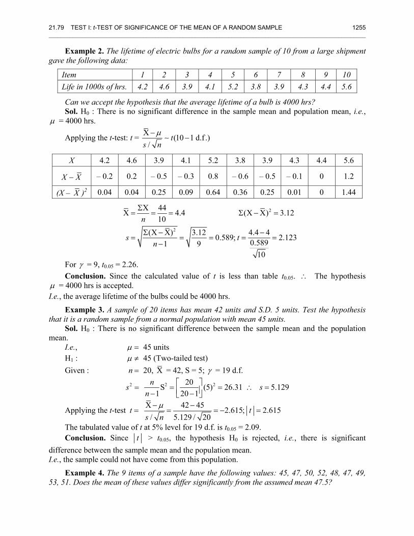
21.79 TEST I: t-TEST OF SIGNIFICANCE OF THE MEAN OF A RANDOM SAMPLE 1255 ________________________________________________________________________________________________________
Example 2. The lifetime of electric bulbs for a random sample of 10 from a large shipment gave the following data:
Item 1 2 3 4 5 6 7 8 9 10 Life in 1000s of hrs. 4.2 4.6 3.9 4.1 5.2 3.8 3.9 4.3 4.4 5.6
Can we accept the hypothesis that the average lifetime of a bulb is 4000 hrs? Sol. H0 : There is no significant difference in the sample mean and population mean, i.e.,
μ = 4000 hrs.
Applying the t-test: t = X (10 1 d.f .)/
ts n
μ−−∼
X 4.2 4.6 3.9 4.1 5.2 3.8 3.9 4.3 4.4 5.6
X X− – 0.2 0.2 – 0.5 – 0.3 0.8 – 0.6 – 0.5 – 0.1 0 1.2
(X – X )2 0.04 0.04 0.25 0.09 0.64 0.36 0.25 0.01 0 1.44
2
2
X 44X 4.4 (X X) 3.1210
(X X) 3.12 4.4 40.589; 2.1230.5891 910
n
s tn
Σ= = = Σ − =
Σ − −= = = = =
−
For γ = 9, t0.05 = 2.26. Conclusion. Since the calculated value of t is less than table t0.05. ∴ The hypothesis
μ = 4000 hrs is accepted. I.e., the average lifetime of the bulbs could be 4000 hrs.
Example 3. A sample of 20 items has mean 42 units and S.D. 5 units. Test the hypothesis that it is a random sample from a normal population with mean 45 units.
Sol. H0 : There is no significant difference between the sample mean and the population mean.
I.e., μ = 45 units H1 : μ ≠ 45 (Two-tailed test) Given : n = 20, X = 42, S = 5; γ = 19 d.f.
2s = 2 220S (5) 26.31 5.1291 20 1
n sn
⎡ ⎤= = ∴ =⎢ ⎥− −⎣ ⎦
Applying the t-test t = X 42 45 2.615; 2.615/ 5.129 / 20
ts n
μ− −= = − =
The tabulated value of t at 5% level for 19 d.f. is t0.05 = 2.09. Conclusion. Since t > t0.05, the hypothesis H0 is rejected, i.e., there is significant
difference between the sample mean and the population mean. I.e., the sample could not have come from this population.
Example 4. The 9 items of a sample have the following values: 45, 47, 50, 52, 48, 47, 49, 53, 51. Does the mean of these values differ significantly from the assumed mean 47.5?
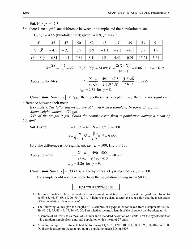
1256 CHAPTER 21: STATISTICS AND PROBABILITY ________________________________________________________________________________________________________
Sol. H0 : μ = 47.5 I.e., there is no significant difference between the sample and the population mean.
H1 : μ ≠ 47.5 (two-tailed test); given : n = 9, μ = 47.5
X 45 47 50 52 48 47 49 53 51
X X− – 4.1 – 2.1 0.9 2.9 – 1.1 – 2.1 – 0.1 3.9 1.9
(X – X )2 16.81 4.41 0.81 8.41 1.21 4.41 0.01 15.21 3.61
2
2 2442 (X X)X= 49.11; (X X) 54.89; 6.86 2.6199 ( 1)
x s sn nΣ Σ −
= = Σ − = = = ∴ =−
Applying the t-test
0.05
X 49.1 47.5 (1.6) 8 1.72792.619/ 2.619 / 8
2.31 for 8.
ts n
t
μ
γ
− −= = = =
= =
Conclusion. Since t < t0.05, the hypothesis is accepted, i.e., there is no significant difference between their mean.
Example 5. The following results are obtained from a sample of 10 boxes of biscuits. Mean weight content = 490 gm. S.D. of the weight 9 gm. Could the sample come from a population having a mean of
500 gm?
Sol. Given:
2 2
10, X 490; S 9 gm, 500
10S 9 9.4861 9
n
nsn
μ= = = =
= = × =−
H0 : The difference is not significant, i.e., μ = 500; H1: 500μ ≠
Applying t-test
0.05
X 490 500 0.333/ 9.486 / 10
2.26 for 9.
ts n
t
μ
γ
− −= = = −
= =
Conclusion. Since t = .333 > t0.05, the hypothesis H0 is rejected, i.e., 500.μ ≠ ∴ The sample could not have come from the population having mean 500 gm.
1. Ten individuals are chosen at random from a normal population of students and their grades are found to be 63, 63, 66, 67, 68, 69, 70, 70, 71, 71. In light of these data, discuss the suggestion that the mean grade of the population of students is 66.
2. The following values give the lengths of 12 samples of Egyptian cotton taken from a shipment: 48, 46, 49, 46, 52, 45, 43, 47, 47, 46, 45, 50. Test whether the mean length of the shipment can be taken as 46.
3. A sample of 18 items has a mean of 24 units and a standard deviation of 3 units. Test the hypothesis that it is a random sample from a normal population with a mean of 27 units.
4. A random sample of 10 students had the following I.Q.’s 70, 120, 110, 101, 88, 83, 95, 98, 107, and 100. Do these data support the assumption of a population mean I.Q. of 160?
TEST YOUR KNOWLEDGE
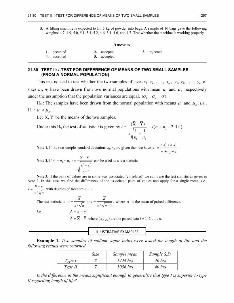
21.80 TEST II: t-TEST FOR DIFFERENCE OF MEANS OF TWO SMALL SAMPLES 1257 ________________________________________________________________________________________________________
5. A filling machine is expected to fill 5 kg of powder into bags. A sample of 10 bags gave the following weights: 4.7, 4.9, 5.0, 5.1, 5.4, 5.2, 4.6, 5.1, 4.6, and 4.7. Test whether the machine is working properly.
Answers 1. accepted 2. accepted 3. rejected 4. accepted 5. accepted
________________________________________________________________________________________________________
21.80 TEST II: t-TEST FOR DIFFERENCE OF MEANS OF TWO SMALL SAMPLES (FROM A NORMAL POPULATION)
This test is used to test whether the two samples of sizes x1, x2, . . . , 1,nx y1, y2, . . . , 2ny of
sizes n1, n2 have been drawn from two normal populations with mean 1μ and 2μ respectively under the assumption that the population variances are equal. 1 2( ).σ σ σ= =
H0 : The samples have been drawn from the normal population with means 1μ and 2μ , i.e., H0 : 1 2.μ μ≠
Let X, Y be the means of the two samples.
Under this H0 the test of statistic t is given by t = 1 2
1 2
(X Y) ( 2 d.f.)1 1
t n ns
n n
−+ −
+∼
Note 1. If the two sample standard deviations s1, s2 are given then we have 2 2
2 1 1 2 2
1 2
.2
n s n ss
n n
+=
+ −
Note 2. If n1 = n2 = n, 2 2
1 2
X Y
1
ts s
n
−=
+
−
can be used as a test statistic.
Note 3. If the pairs of values are in some way associated (correlated) we can’t use the test statistic as given in Note 2. In this case we find the differences of the associated pairs of values and apply for a single mean, i.e.,
X
/t
s n
μ−= with degrees of freedom n – 1.
The test statistic is /
dt
s n= or ,
/ 1
dt
s n=
− where d is the mean of paired difference.
I.e.,
X Y, where ( , ) are the paired data 1, 2, . . . , .i i i
i i i
d x y
d x y i n
= −
= − =
Example 1. Two samples of sodium vapor bulbs were tested for length of life and the following results were returned:
Size Sample mean Sample S.D. Type I 8 1234 hrs 36 hrs Type II 7 1036 hrs 40 hrs
Is the difference in the means significant enough to generalize that type I is superior to type II regarding length of life?
ILLUSTRATIVE EXAMPLES
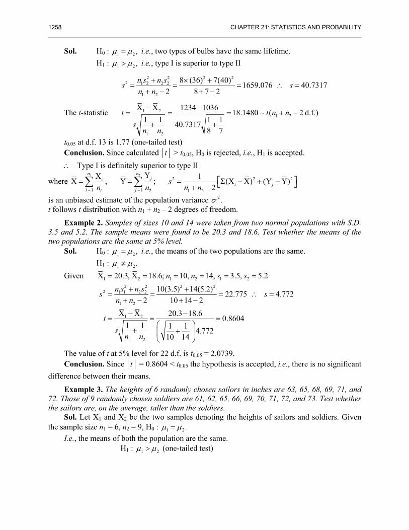
1258 CHAPTER 21: STATISTICS AND PROBABILITY ________________________________________________________________________________________________________
Sol. H0 : 1 2 ,μ μ= i.e., two types of bulbs have the same lifetime. H1 : 1 2 ,μ μ> i.e., type I is superior to type II
2 2 2 2
2 1 2 2 2
1 2
8 (36) 7(40) 1659.076 40.73172 8 7 2
n s n ss sn n
+ × += = = ∴ =
+ − + −
The t-statistic 1 21 2
1 2
X X 1234 1036 18.1480 ( 2 d.f.)1 1 1 140.7317
8 7
t t n ns
n n
− −= = = + −
+ +∼
t0.05 at d.f. 13 is 1.77 (one-tailed test) Conclusion. Since calculated t > t0.05, H0 is rejected, i.e., H1 is accepted. ∴ Type I is definitely superior to type II
where 1 2
2 2 2
1 1 2 1 2
YX 1X , Y ; (X X) (Y Y)2
n nji
i ji ji
sn n n n= =
⎡ ⎤= = = Σ − + −⎣ ⎦+ −∑ ∑
is an unbiased estimate of the population variance 2.σ t follows t distribution with n1 + n2 – 2 degrees of freedom.
Example 2. Samples of sizes 10 and 14 were taken from two normal populations with S.D. 3.5 and 5.2. The sample means were found to be 20.3 and 18.6. Test whether the means of the two populations are the same at 5% level.
Sol. H0 : 1 2 ,μ μ= i.e., the means of the two populations are the same. H1 : 1 2.μ μ≠ Given 1 2 1 2 1 2
2 2 2 22 1 1 2 2
1 2
1 2
1 2
X 20.3, X 18.6; 10, 14, 3.5, 5.2
10(3.5) 14(5.2) 22.775 4.7722 10 14 2
X X 20.3 18.6 0.86041 1 1 1 4.772
10 14
n n s s
n s n ss sn n
ts
n n
= = = = = =
+ += = = ∴ =
+ − + −
− −= = =
⎛ ⎞+ +⎜ ⎟
⎝ ⎠
The value of t at 5% level for 22 d.f. is t0.05 = 2.0739. Conclusion. Since t = 0.8604 < t0.05 the hypothesis is accepted, i.e., there is no significant
difference between their means.
Example 3. The heights of 6 randomly chosen sailors in inches are 63, 65, 68, 69, 71, and 72. Those of 9 randomly chosen soldiers are 61, 62, 65, 66, 69, 70, 71, 72, and 73. Test whether the sailors are, on the average, taller than the soldiers.
Sol. Let X1 and X2 be the two samples denoting the heights of sailors and soldiers. Given the sample size n1 = 6, n2 = 9, H0 : 1 2.μ μ=
I.e., the means of both the population are the same. H1 : 1 2μ μ> (one-tailed test)
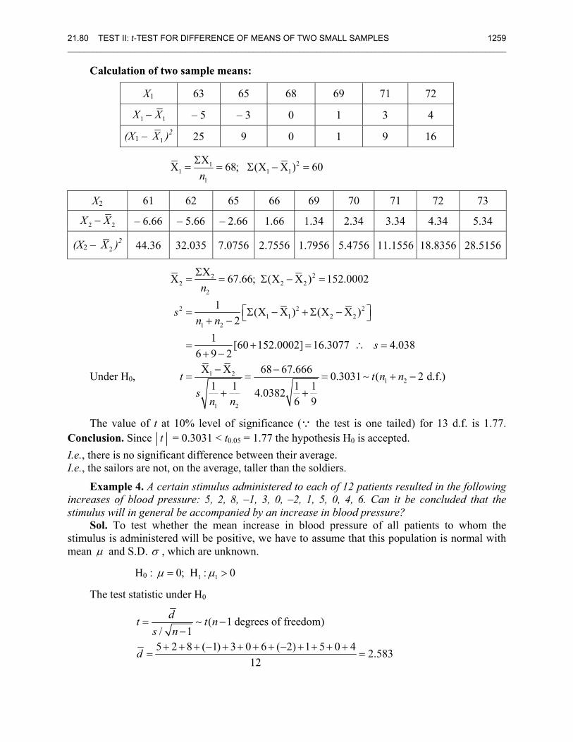
21.80 TEST II: t-TEST FOR DIFFERENCE OF MEANS OF TWO SMALL SAMPLES 1259 ________________________________________________________________________________________________________
Calculation of two sample means:
X1 63 65 68 69 71 72
1 1X X− – 5 – 3 0 1 3 4
(X1 – 1X )2 25 9 0 1 9 16
211 1 1
1
XX 68; (X X ) 60nΣ
= = Σ − =
X2 61 62 65 66 69 70 71 72 73
2 2X X− – 6.66 – 5.66 – 2.66 1.66 1.34 2.34 3.34 4.34 5.34
(X2 – 2X )2 44.36 32.035 7.0756 2.7556 1.7956 5.4756 11.1556 18.8356 28.5156
Under H0,
222 2 2
2
2 2 21 1 2 2
1 2
1 21 2
1 2
XX 67.66; (X X ) 152.0002
1 (X X ) (X X )2
1 [60 152.0002] 16.3077 4.0386 9 2X X 68 67.666 0.3031 ( 2 d.f.)
1 1 1 14.03826 9
n
sn n
s
t t n ns
n n
Σ= = Σ − =
⎡ ⎤= Σ − +Σ −⎣ ⎦+ −
= + = ∴ =+ −− −
= = = + −+ +
∼
The value of t at 10% level of significance (∵ the test is one tailed) for 13 d.f. is 1.77. Conclusion. Since t = 0.3031 < t0.05 = 1.77 the hypothesis H0 is accepted. I.e., there is no significant difference between their average. I.e., the sailors are not, on the average, taller than the soldiers.
Example 4. A certain stimulus administered to each of 12 patients resulted in the following increases of blood pressure: 5, 2, 8, –1, 3, 0, –2, 1, 5, 0, 4, 6. Can it be concluded that the stimulus will in general be accompanied by an increase in blood pressure?
Sol. To test whether the mean increase in blood pressure of all patients to whom the stimulus is administered will be positive, we have to assume that this population is normal with mean μ and S.D. σ , which are unknown.
H0 : 1 10; H : 0μ μ= >
The test statistic under H0
( 1 degrees of freedom)
/ 15 2 8 ( 1) 3 0 6 ( 2) 1 5 0 4 2.583
12
dt t ns n
d
= −−
+ + + − + + + + − + + + += =
∼
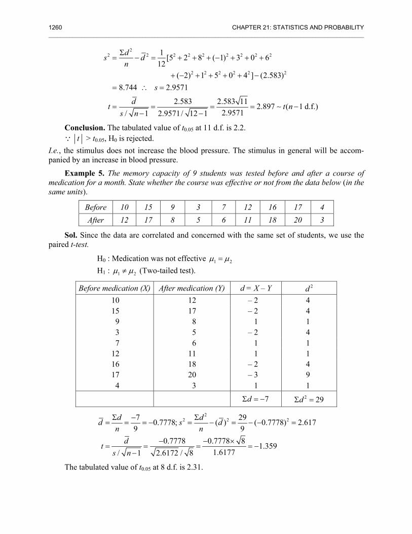
1260 CHAPTER 21: STATISTICS AND PROBABILITY ________________________________________________________________________________________________________
22 2 2 2 2 2 2 2 2
2 2 2 2 2 2
1 [5 2 8 ( 1) 3 0 612
( 2) 1 5 0 4 ] (2.583)8.744 2.9571
2.583 2.583 11 2.897 ( 1 d.f.)2.9571/ 1 2.9571/ 12 1
ds dn
s
dt t ns n
Σ= − = + + + − + + +
+ − + + + + −= ∴ =
= = = = −− −
∼
Conclusion. The tabulated value of t0.05 at 11 d.f. is 2.2. t∵ > t0.05, H0 is rejected.
I.e., the stimulus does not increase the blood pressure. The stimulus in general will be accom-panied by an increase in blood pressure.
Example 5. The memory capacity of 9 students was tested before and after a course of medication for a month. State whether the course was effective or not from the data below (in the same units).
Before 10 15 9 3 7 12 16 17 4 After 12 17 8 5 6 11 18 20 3
Sol. Since the data are correlated and concerned with the same set of students, we use the paired t-test.
H0 : Medication was not effective 1 2μ μ= H1 : 1 2μ μ≠ (Two-tailed test).
Before medication (X) After medication (Y) d = X – Y 2d 10 12 – 2 4 15 17 – 2 4 9 8 1 1 3 5 – 2 4 7 6 1 1
12 11 1 1 16 18 – 2 4 17 20 – 3 9 4 3 1 1
7dΣ = − 2 29dΣ =
22 2 27 290.7778; ( ) ( 0.7778) 2.617
9 90.7778 0.7778 8 1.359
1.6177/ 1 2.6172 / 8
d dd s dn n
dts n
Σ − Σ= = = − = − = − − =
− − ×= = = = −
−
The tabulated value of t0.05 at 8 d.f. is 2.31.
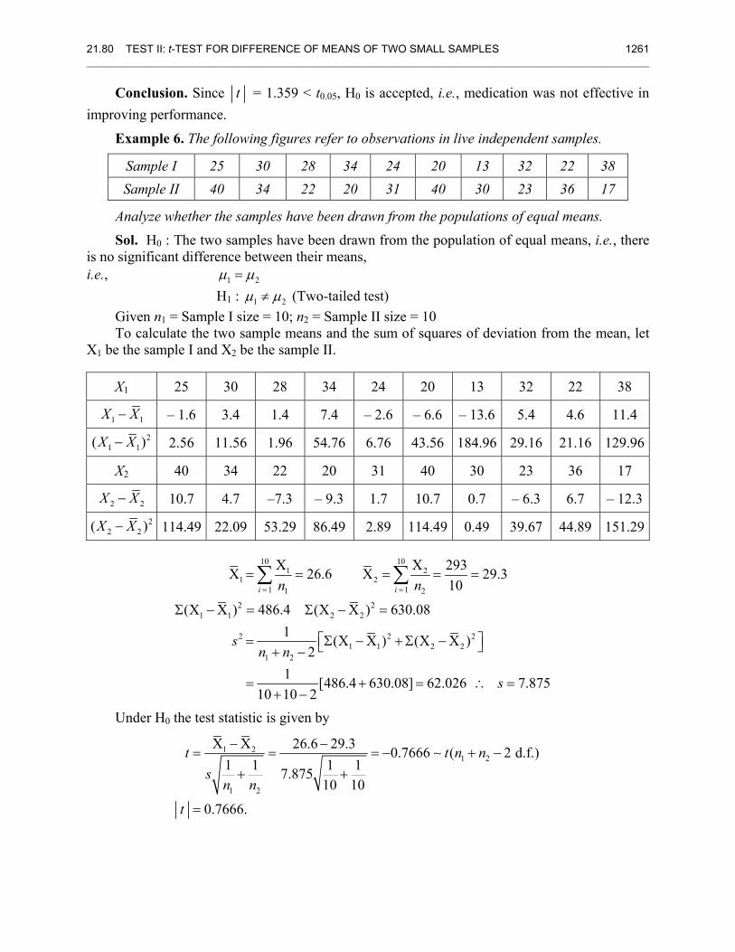
21.80 TEST II: t-TEST FOR DIFFERENCE OF MEANS OF TWO SMALL SAMPLES 1261 ________________________________________________________________________________________________________
Conclusion. Since t = 1.359 < t0.05, H0 is accepted, i.e., medication was not effective in improving performance.
Example 6. The following figures refer to observations in live independent samples.
Sample I 25 30 28 34 24 20 13 32 22 38 Sample II 40 34 22 20 31 40 30 23 36 17
Analyze whether the samples have been drawn from the populations of equal means.
Sol. H0 : The two samples have been drawn from the population of equal means, i.e., there is no significant difference between their means, i.e., 1 2μ μ= H1 : 1 2μ μ≠ (Two-tailed test)
Given n1 = Sample I size = 10; n2 = Sample II size = 10 To calculate the two sample means and the sum of squares of deviation from the mean, let
X1 be the sample I and X2 be the sample II.
X1 25 30 28 34 24 20 13 32 22 38
1 1X X− – 1.6 3.4 1.4 7.4 – 2.6 – 6.6 – 13.6 5.4 4.6 11.4 2
1 1( )X X− 2.56 11.56 1.96 54.76 6.76 43.56 184.96 29.16 21.16 129.96
X2 40 34 22 20 31 40 30 23 36 17
2 2X X− 10.7 4.7 –7.3 – 9.3 1.7 10.7 0.7 – 6.3 6.7 – 12.32
2 2( )X X− 114.49 22.09 53.29 86.49 2.89 114.49 0.49 39.67 44.89 151.29
10 101 2
1 21 11 2
2 21 1 2 2
2 2 21 1 2 2
1 2
X X 293X 26.6 X 29.310
(X X ) 486.4 (X X ) 630.081 (X X ) (X X )
21 [486.4 630.08] 62.026 7.875
10 10 2
i in n
sn n
s
= =
= = = = =
Σ − = Σ − =
⎡ ⎤= Σ − + Σ −⎣ ⎦+ −
= + = ∴ =+ −
∑ ∑
Under H0 the test statistic is given by
1 21 2
1 2
X X 26.6 29.3 0.7666 ( 2 d.f.)1 1 1 17.875
10 10
0.7666.
t t n ns
n n
t
− −= = = − + −
+ +
=
∼
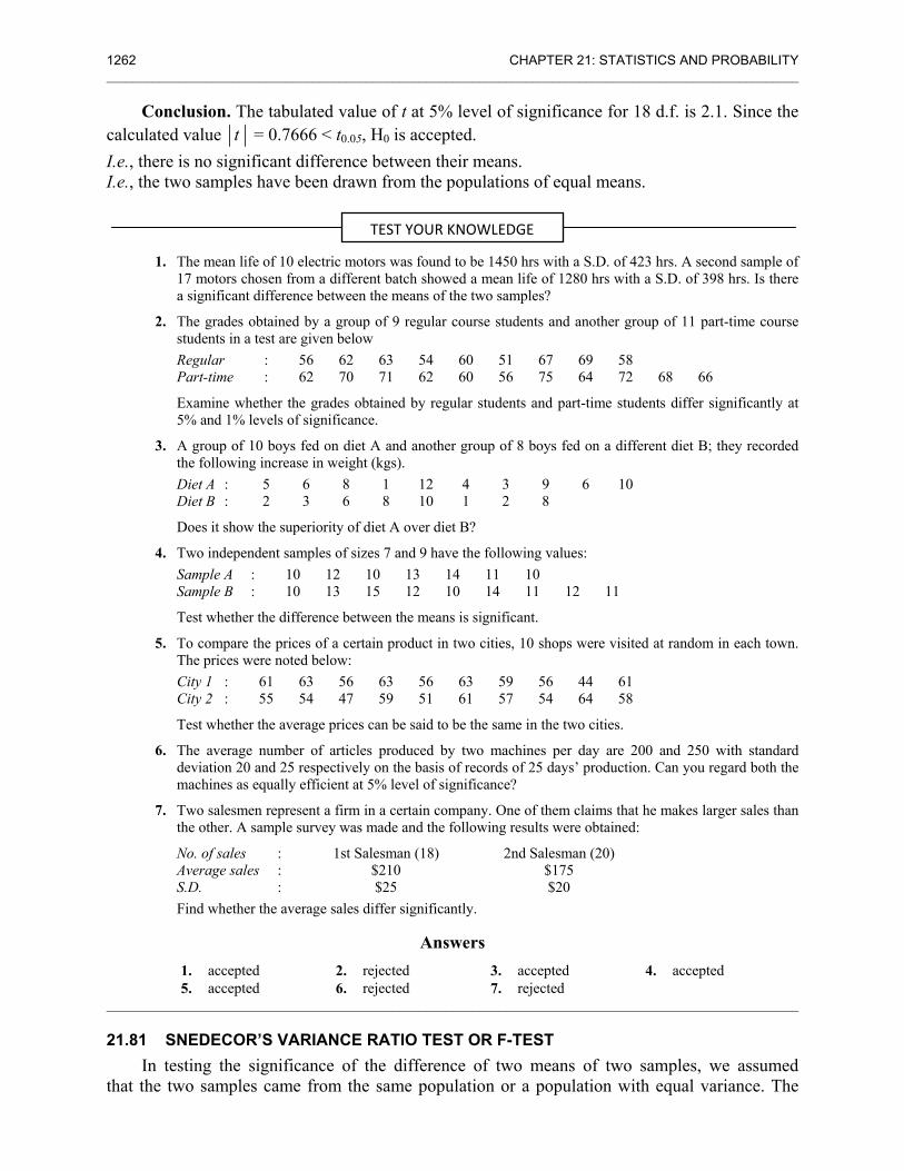
1262 CHAPTER 21: STATISTICS AND PROBABILITY ________________________________________________________________________________________________________
Conclusion. The tabulated value of t at 5% level of significance for 18 d.f. is 2.1. Since the calculated value t = 0.7666 < t0.05, H0 is accepted. I.e., there is no significant difference between their means. I.e., the two samples have been drawn from the populations of equal means.
1. The mean life of 10 electric motors was found to be 1450 hrs with a S.D. of 423 hrs. A second sample of 17 motors chosen from a different batch showed a mean life of 1280 hrs with a S.D. of 398 hrs. Is there a significant difference between the means of the two samples?
2. The grades obtained by a group of 9 regular course students and another group of 11 part-time course students in a test are given below
Regular : 56 62 63 54 60 51 67 69 58 Part-time : 62 70 71 62 60 56 75 64 72 68 66
Examine whether the grades obtained by regular students and part-time students differ significantly at 5% and 1% levels of significance.
3. A group of 10 boys fed on diet A and another group of 8 boys fed on a different diet B; they recorded the following increase in weight (kgs).
Diet A : 5 6 8 1 12 4 3 9 6 10 Diet B : 2 3 6 8 10 1 2 8
Does it show the superiority of diet A over diet B?
4. Two independent samples of sizes 7 and 9 have the following values: Sample A : 10 12 10 13 14 11 10 Sample B : 10 13 15 12 10 14 11 12 11
Test whether the difference between the means is significant.
5. To compare the prices of a certain product in two cities, 10 shops were visited at random in each town. The prices were noted below:
City 1 : 61 63 56 63 56 63 59 56 44 61 City 2 : 55 54 47 59 51 61 57 54 64 58
Test whether the average prices can be said to be the same in the two cities.
6. The average number of articles produced by two machines per day are 200 and 250 with standard deviation 20 and 25 respectively on the basis of records of 25 days’ production. Can you regard both the machines as equally efficient at 5% level of significance?
7. Two salesmen represent a firm in a certain company. One of them claims that he makes larger sales than the other. A sample survey was made and the following results were obtained:
No. of sales : 1st Salesman (18) 2nd Salesman (20) Average sales : $210 $175 S.D. : $25 $20 Find whether the average sales differ significantly.
Answers 1. accepted 2. rejected 3. accepted 4. accepted 5. accepted 6. rejected 7. rejected
________________________________________________________________________________________________________
21.81 SNEDECOR’S VARIANCE RATIO TEST OR F-TEST In testing the significance of the difference of two means of two samples, we assumed
that the two samples came from the same population or a population with equal variance. The
TEST YOUR KNOWLEDGE
21.81 SNEDECOR’S VARIANCE RATIO TEST OR F-TEST 1263 ________________________________________________________________________________________________________
object of the F-test is to discover whether two independent estimates of population variance differ significantly or whether the two samples may be regarded as drawn from the normal populations having the same variance. Hence before applying the t-test for the significance of the difference of two means, we have to test for the equality of population variance by using the F-test.
Let n1 and n2 be the sizes of two samples with variance 21s and 2
2 .s The estimates of the
population variance based on these samples are 2
2 1 11
1 1n ssn
=−
and 2
2 2 22
2
.1
n ssn
=−
The degrees of
freedom of these estimates are 1 1 2 21, 1.v n v n= − = − To test whether these estimates 2
1s and 22s are significantly different or whether the samples
may be regarded as drawn from the same population or from two populations with the same variance 2 ,σ we set up the null hypothesis H0 : 2 2 2
1 2 .σ σ σ= = I.e., the independent estimates of the common population do not differ significantly.
To carry out the test of significance of the difference of the variances we calculate the test
statistic (Nr) F = 2122
;ss
the numerator is greater than the denominator (Dr), i.e., 2 21 2 .s s>
Conclusion. If the calculated value of F exceeds F0.05 for (n1 – 1), (n2 – 1) degrees of freedom given in the table we conclude that the ratio is significant at 5% level. I.e., we conclude that the sample could have come from two normal populations with the same variance.
The assumptions on which the F-test is based are:
1. The populations for each sample must be normally distributed. 2. The samples must be random and independent. 3. The ratio of 2
1σ to 22σ should be equal to 1 or greater than 1. That is why we take the
larger variance in the numerator of the ratio.
Applications. The F-test is used to test (i) whether two independent samples have been drawn from the normal populations with
the same variance 2.σ (ii) Whether the two independent estimates of the population variance are homogeneous or
not.
Example 1. In two independent samples of sizes 8 and 10 the sum of squares of deviations of the sample values from the respective sample means were 84.4 and 102.6. Test whether the difference of variances of the populations is significant or not.
Sol. Null hypothesis H0. 2 2 21 2 ,σ σ σ= = i.e., there is no significant difference between
population variance.
Under H0 : 21
1 222
F F( , d.f.)s v vs
= ∼
ILLUSTRATIVE EXAMPLES
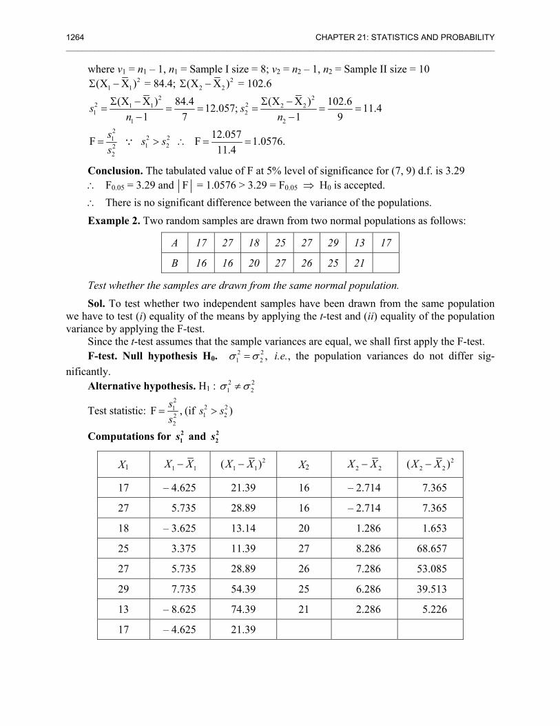
1264 CHAPTER 21: STATISTICS AND PROBABILITY ________________________________________________________________________________________________________
where v1 = n1 – 1, n1 = Sample I size = 8; v2 = n2 – 1, n2 = Sample II size = 10 2
1 1(X X )Σ − = 84.4; 22 2(X X )Σ − = 102.6
2 22 21 1 2 21 2
1 2
(X X ) (X X )84.4 102.612.057; 11.41 7 1 9
s sn n
Σ − Σ −= = = = = =
− − 2
2 211 22
2
12.057F F 1.0576.11.4
s s ss
= > ∴ = =∵
Conclusion. The tabulated value of F at 5% level of significance for (7, 9) d.f. is 3.29 ∴ F0.05 = 3.29 and F = 1.0576 > 3.29 = F0.05 ⇒ H0 is accepted. ∴ There is no significant difference between the variance of the populations.
Example 2. Two random samples are drawn from two normal populations as follows:
A 17 27 18 25 27 29 13 17
B 16 16 20 27 26 25 21
Test whether the samples are drawn from the same normal population.
Sol. To test whether two independent samples have been drawn from the same population we have to test (i) equality of the means by applying the t-test and (ii) equality of the population variance by applying the F-test.
Since the t-test assumes that the sample variances are equal, we shall first apply the F-test. F-test. Null hypothesis H0. 2 2
1 2 ,σ σ= i.e., the population variances do not differ sig-nificantly.
Alternative hypothesis. H1 : 2 21 2σ σ≠
Test statistic: 2
2 211 22
2
F , (if )s s ss
= >
Computations for 21s and 2
2s
X1 1 1X X− 21 1( )X X− X2 2 2X X− 2
2 2( )X X−
17 – 4.625 21.39 16 – 2.714 7.365
27 5.735 28.89 16 – 2.714 7.365
18 – 3.625 13.14 20 1.286 1.653
25 3.375 11.39 27 8.286 68.657
27 5.735 28.89 26 7.286 53.085
29 7.735 54.39 25 6.286 39.513
13 – 8.625 74.39 21 2.286 5.226
17 – 4.625 21.39
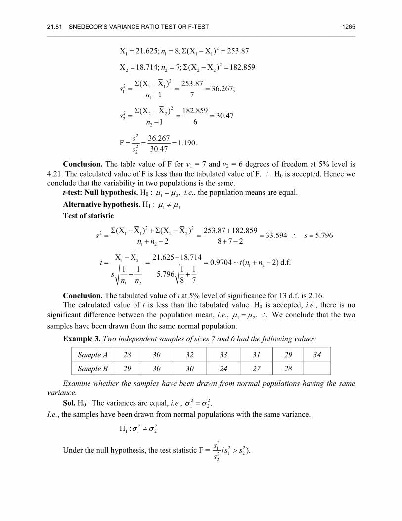
21.81 SNEDECOR’S VARIANCE RATIO TEST OR F-TEST 1265 ________________________________________________________________________________________________________
21 1 1 1
22 2 2 2
22 1 11
1
22 2 22
2
2122
X 21.625; 8; (X X ) 253.87
X 18.714; 7; (X X ) 182.859
(X X ) 253.87 36.267;1 7
(X X ) 182.859 30.471 6
36.267F 1.190.30.47
n
n
sn
sn
ss
= = Σ − =
= = Σ − =
Σ −= = =
−
Σ −= = =
−
= = =
Conclusion. The table value of F for v1 = 7 and v2 = 6 degrees of freedom at 5% level is 4.21. The calculated value of F is less than the tabulated value of F. ∴ H0 is accepted. Hence we conclude that the variability in two populations is the same.
t-test: Null hypothesis. H0 : 1 2 ,μ μ= i.e., the population means are equal. Alternative hypothesis. H1 : 1 2μ μ≠ Test of statistic
2 22 1 1 2 2
1 2
1 21 2
1 2
(X X ) (X X ) 253.87 182.859 33.594 5.7962 8 7 2
X X 21.625 18.714 0.9704 ( 2) d.f.1 1 1 15.796
8 7
s sn n
t t n ns
n n
Σ − +Σ − += = = ∴ =
+ − + −
− −= = = + −
+ +∼
Conclusion. The tabulated value of t at 5% level of significance for 13 d.f. is 2.16. The calculated value of t is less than the tabulated value. H0 is accepted, i.e., there is no
significant difference between the population mean, i.e., 1 2.μ μ= ∴ We conclude that the two samples have been drawn from the same normal population.
Example 3. Two independent samples of sizes 7 and 6 had the following values:
Sample A 28 30 32 33 31 29 34
Sample B 29 30 30 24 27 28
Examine whether the samples have been drawn from normal populations having the same variance.
Sol. H0 : The variances are equal, i.e., 2 21 2 .σ σ=
I.e., the samples have been drawn from normal populations with the same variance.
2 21 1 2H :σ σ≠
Under the null hypothesis, the test statistic F = 2
2 211 22
2
( ).s s ss
>
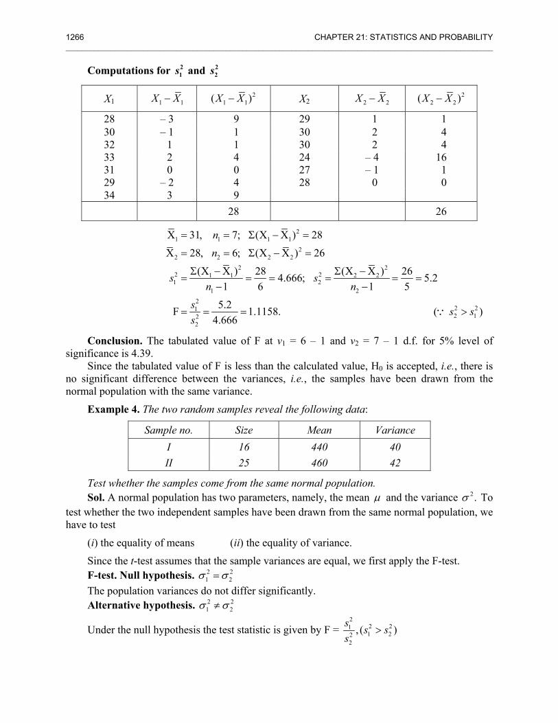
1266 CHAPTER 21: STATISTICS AND PROBABILITY ________________________________________________________________________________________________________
Computations for 21s and 2
2s
X1 1 1X X− 21 1( )X X− X2 2 2X X− 2
2 2( )X X−
28 – 3 9 29 1 1 30 – 1 1 30 2 4 32 1 1 30 2 4 33 2 4 24 – 4 16 31 0 0 27 – 1 1 29 – 2 4 28 0 0 34 3 9 28 26
21 1 1 1
22 2 2 2
2 22 21 1 2 21 2
1 22
2 212 12
2
X 31, 7; (X X ) 28
X 28, 6; (X X ) 26
(X X ) (X X )28 264.666; 5.21 6 1 5
5.2F 1.1158. ( )4.666
n
n
s sn n
s s ss
= = Σ − =
= = Σ − =
Σ − Σ −= = = = = =
− −
= = = >∵
Conclusion. The tabulated value of F at v1 = 6 – 1 and v2 = 7 – 1 d.f. for 5% level of significance is 4.39.
Since the tabulated value of F is less than the calculated value, H0 is accepted, i.e., there is no significant difference between the variances, i.e., the samples have been drawn from the normal population with the same variance.
Example 4. The two random samples reveal the following data:
Sample no. Size Mean Variance I 16 440 40 II 25 460 42
Test whether the samples come from the same normal population. Sol. A normal population has two parameters, namely, the mean μ and the variance 2.σ To
test whether the two independent samples have been drawn from the same normal population, we have to test
(i) the equality of means (ii) the equality of variance.
Since the t-test assumes that the sample variances are equal, we first apply the F-test. F-test. Null hypothesis. 2 2
1 2σ σ= The population variances do not differ significantly. Alternative hypothesis. 2 2
1 2σ σ≠
Under the null hypothesis the test statistic is given by F = 2
2 211 22
2
, ( )s s ss
>
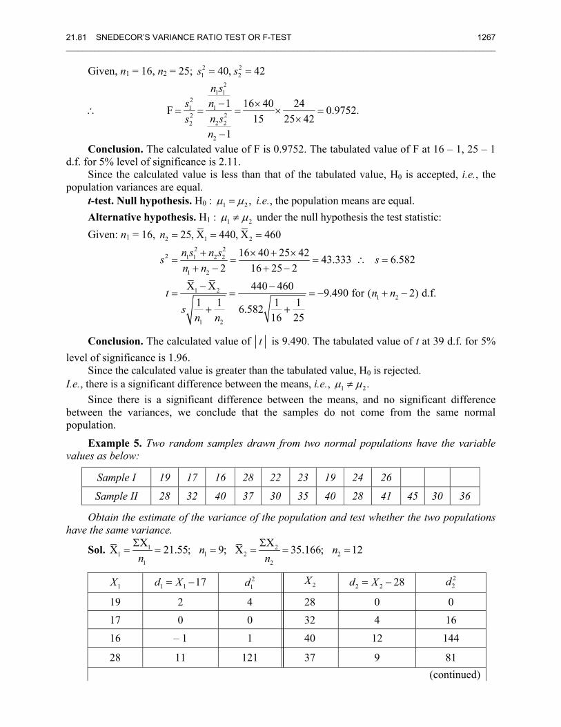
21.81 SNEDECOR’S VARIANCE RATIO TEST OR F-TEST 1267 ________________________________________________________________________________________________________
Given, n1 = 16, n2 = 25; 2 21 240, 42s s= =
∴
21 1
21 1
222 22
2
1 16 40 24F 0.9752.15 25 42
1
n ss n
n ssn
− ×= = = × =
×−
Conclusion. The calculated value of F is 0.9752. The tabulated value of F at 16 – 1, 25 – 1 d.f. for 5% level of significance is 2.11.
Since the calculated value is less than that of the tabulated value, H0 is accepted, i.e., the population variances are equal.
t-test. Null hypothesis. H0 : 1 2 ,μ μ= i.e., the population means are equal. Alternative hypothesis. H1 : 1 2μ μ≠ under the null hypothesis the test statistic: Given: n1 = 16, 2 1 2
2 22 1 1 2 2
1 2
1 21 2
1 2
25, X 440, X 460
16 40 25 42 43.333 6.5822 16 25 2
X X 440 460 9.490 for ( 2) d.f.1 1 1 16.582
16 25
n
n s n ss sn n
t n ns
n n
= = =
+ × + ×= = = ∴ =
+ − + −
− −= = = − + −
+ +
Conclusion. The calculated value of t is 9.490. The tabulated value of t at 39 d.f. for 5% level of significance is 1.96.
Since the calculated value is greater than the tabulated value, H0 is rejected. I.e., there is a significant difference between the means, i.e., 1 2.μ μ≠
Since there is a significant difference between the means, and no significant difference between the variances, we conclude that the samples do not come from the same normal population.
Example 5. Two random samples drawn from two normal populations have the variable values as below:
Sample I 19 17 16 28 22 23 19 24 26
Sample II 28 32 40 37 30 35 40 28 41 45 30 36
Obtain the estimate of the variance of the population and test whether the two populations have the same variance.
Sol. 1 21 1 2 2
1 2
X XX 21.55; 9; X 35.166; 12n nn nΣ Σ
= = = = = =
1X 1 1 17d X= − 2
1d 2X 2 2 28d X= − 22d
19 2 4 28 0 0 17 0 0 32 4 16
16 – 1 1 40 12 144
28 11 121 37 9 81 (continued)
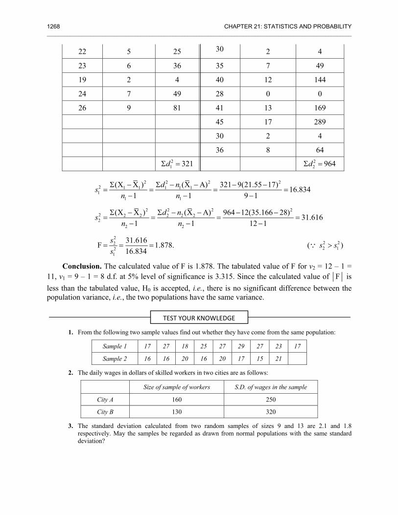
1268 CHAPTER 21: STATISTICS AND PROBABILITY ________________________________________________________________________________________________________
22 5 25 30 2 4
23 6 36 35 7 49
19 2 4 40 12 144
24 7 49 28 0 0
26 9 81 41 13 169
45 17 289
30 2 4
36 8 64
21 321dΣ = 2
2 964dΣ =
2 2 2 22 1 1 1 1 11
1 1
2 2 2 22 2 2 2 2 22
2 2
22 222 12
1
(X X ) (X A) 321 9(21.55 17) 16.8341 1 9 1
(X X ) (X A) 964 12(35.166 28) 31.6161 1 12 1
31.616F 1.878. ( )16.834
d nsn n
d nsn n
s s ss
Σ − Σ − − − −= = = =
− − −
Σ − Σ − − − −= = = =
− − −
= = = >∵
Conclusion. The calculated value of F is 1.878. The tabulated value of F for v2 = 12 – 1 = 11, v1 = 9 – 1 = 8 d.f. at 5% level of significance is 3.315. Since the calculated value of F is less than the tabulated value, H0 is accepted, i.e., there is no significant difference between the population variance, i.e., the two populations have the same variance.
1. From the following two sample values find out whether they have come from the same population:
Sample 1 17 27 18 25 27 29 27 23 17
Sample 2 16 16 20 16 20 17 15 21
2. The daily wages in dollars of skilled workers in two cities are as follows:
Size of sample of workers S.D. of wages in the sample
City A 160 250
City B 130 320
3. The standard deviation calculated from two random samples of sizes 9 and 13 are 2.1 and 1.8 respectively. May the samples be regarded as drawn from normal populations with the same standard deviation?
TEST YOUR KNOWLEDGE
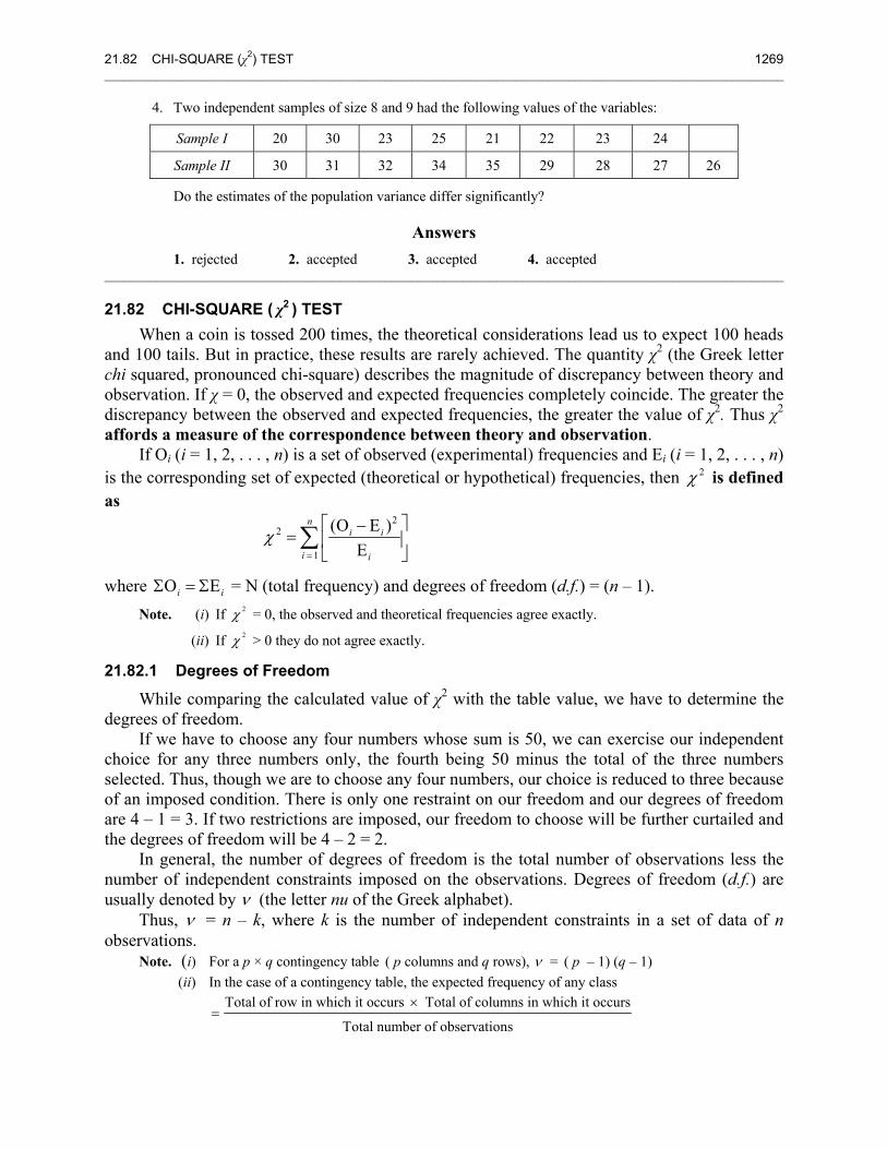
21.82 CHI-SQUARE (χ2) TEST 1269 ________________________________________________________________________________________________________
4. Two independent samples of size 8 and 9 had the following values of the variables:
Sample I 20 30 23 25 21 22 23 24
Sample II 30 31 32 34 35 29 28 27 26
Do the estimates of the population variance differ significantly?
Answers 1. rejected 2. accepted 3. accepted 4. accepted ________________________________________________________________________________________________________
21.82 CHI-SQUARE ( χ2 ) TEST When a coin is tossed 200 times, the theoretical considerations lead us to expect 100 heads
and 100 tails. But in practice, these results are rarely achieved. The quantity χ2 (the Greek letter chi squared, pronounced chi-square) describes the magnitude of discrepancy between theory and observation. If χ = 0, the observed and expected frequencies completely coincide. The greater the discrepancy between the observed and expected frequencies, the greater the value of χ2. Thus χ2 affords a measure of the correspondence between theory and observation.
If Oi (i = 1, 2, . . . , n) is a set of observed (experimental) frequencies and Ei (i = 1, 2, . . . , n) is the corresponding set of expected (theoretical or hypothetical) frequencies, then 2χ is defined as
2
2
1
(O E )E
ni i
i i
χ=
⎡ ⎤−= ⎢ ⎥
⎣ ⎦∑
where O Ei iΣ = Σ = N (total frequency) and degrees of freedom (d.f.) = (n – 1). Note. (i) If 2χ = 0, the observed and theoretical frequencies agree exactly.
(ii) If 2χ > 0 they do not agree exactly.
21.82.1 Degrees of Freedom
While comparing the calculated value of χ2 with the table value, we have to determine the degrees of freedom.
If we have to choose any four numbers whose sum is 50, we can exercise our independent choice for any three numbers only, the fourth being 50 minus the total of the three numbers selected. Thus, though we are to choose any four numbers, our choice is reduced to three because of an imposed condition. There is only one restraint on our freedom and our degrees of freedom are 4 – 1 = 3. If two restrictions are imposed, our freedom to choose will be further curtailed and the degrees of freedom will be 4 – 2 = 2.
In general, the number of degrees of freedom is the total number of observations less the number of independent constraints imposed on the observations. Degrees of freedom (d.f.) are usually denoted by ν (the letter nu of the Greek alphabet).
Thus, ν = n – k, where k is the number of independent constraints in a set of data of n observations.
Note. (i) For a p × q contingency table ( p columns and q rows), ν = ( p – 1) (q – 1) (ii) In the case of a contingency table, the expected frequency of any class
Total of row in which it occurs Total of columns in which it occurs
Total number of observations
×=
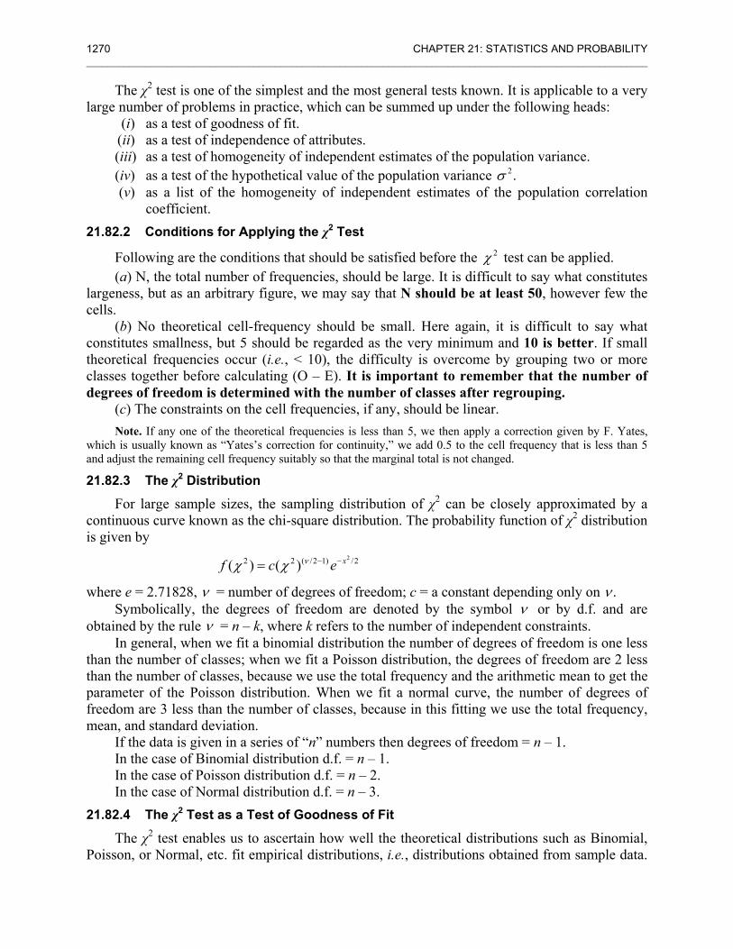
1270 CHAPTER 21: STATISTICS AND PROBABILITY ________________________________________________________________________________________________________
The χ2 test is one of the simplest and the most general tests known. It is applicable to a very large number of problems in practice, which can be summed up under the following heads:
(i) as a test of goodness of fit. (ii) as a test of independence of attributes. (iii) as a test of homogeneity of independent estimates of the population variance. (iv) as a test of the hypothetical value of the population variance 2.σ (v) as a list of the homogeneity of independent estimates of the population correlation
coefficient. 21.82.2 Conditions for Applying the χ2 Test
Following are the conditions that should be satisfied before the 2χ test can be applied. (a) N, the total number of frequencies, should be large. It is difficult to say what constitutes
largeness, but as an arbitrary figure, we may say that N should be at least 50, however few the cells.
(b) No theoretical cell-frequency should be small. Here again, it is difficult to say what constitutes smallness, but 5 should be regarded as the very minimum and 10 is better. If small theoretical frequencies occur (i.e., < 10), the difficulty is overcome by grouping two or more classes together before calculating (O – E). It is important to remember that the number of degrees of freedom is determined with the number of classes after regrouping.
(c) The constraints on the cell frequencies, if any, should be linear. Note. If any one of the theoretical frequencies is less than 5, we then apply a correction given by F. Yates,
which is usually known as “Yates’s correction for continuity,” we add 0.5 to the cell frequency that is less than 5 and adjust the remaining cell frequency suitably so that the marginal total is not changed.
21.82.3 The χ2 Distribution
For large sample sizes, the sampling distribution of χ2 can be closely approximated by a continuous curve known as the chi-square distribution. The probability function of χ2 distribution is given by
22 2 ( /2 1) /2( ) ( ) xf c eνχ χ − −=
where e = 2.71828, ν = number of degrees of freedom; c = a constant depending only on .ν Symbolically, the degrees of freedom are denoted by the symbol ν or by d.f. and are
obtained by the rule ν = n – k, where k refers to the number of independent constraints. In general, when we fit a binomial distribution the number of degrees of freedom is one less
than the number of classes; when we fit a Poisson distribution, the degrees of freedom are 2 less than the number of classes, because we use the total frequency and the arithmetic mean to get the parameter of the Poisson distribution. When we fit a normal curve, the number of degrees of freedom are 3 less than the number of classes, because in this fitting we use the total frequency, mean, and standard deviation.
If the data is given in a series of “n” numbers then degrees of freedom = n – 1. In the case of Binomial distribution d.f. = n – 1. In the case of Poisson distribution d.f. = n – 2. In the case of Normal distribution d.f. = n – 3.
21.82.4 The χ2 Test as a Test of Goodness of Fit
The χ2 test enables us to ascertain how well the theoretical distributions such as Binomial, Poisson, or Normal, etc. fit empirical distributions, i.e., distributions obtained from sample data.
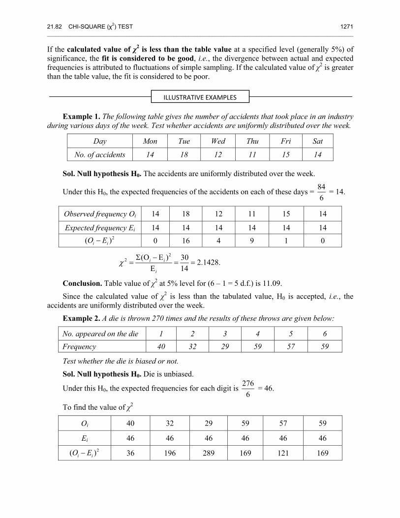
21.82 CHI-SQUARE (χ2) TEST 1271 ________________________________________________________________________________________________________
If the calculated value of χ2 is less than the table value at a specified level (generally 5%) of significance, the fit is considered to be good, i.e., the divergence between actual and expected frequencies is attributed to fluctuations of simple sampling. If the calculated value of χ2 is greater than the table value, the fit is considered to be poor.
Example 1. The following table gives the number of accidents that took place in an industry during various days of the week. Test whether accidents are uniformly distributed over the week.
Day Mon Tue Wed Thu Fri Sat
No. of accidents 14 18 12 11 15 14
Sol. Null hypothesis H0. The accidents are uniformly distributed over the week.
Under this H0, the expected frequencies of the accidents on each of these days = 846
= 14.
Observed frequency Oi 14 18 12 11 15 14
Expected frequency Ei 14 14 14 14 14 14 2( )i iO E− 0 16 4 9 1 0
2
2 (O E ) 30 2.1428.E 14i i
i
χ Σ −= = =
Conclusion. Table value of χ2 at 5% level for (6 – 1 = 5 d.f.) is 11.09.
Since the calculated value of χ2 is less than the tabulated value, H0 is accepted, i.e., the accidents are uniformly distributed over the week.
Example 2. A die is thrown 270 times and the results of these throws are given below:
No. appeared on the die 1 2 3 4 5 6 Frequency 40 32 29 59 57 59
Test whether the die is biased or not.
Sol. Null hypothesis H0. Die is unbiased.
Under this H0, the expected frequencies for each digit is 2766
= 46.
To find the value of χ2
Oi 40 32 29 59 57 59
Ei 46 46 46 46 46 46 2( )i iO E− 36 196 289 169 121 169
ILLUSTRATIVE EXAMPLES
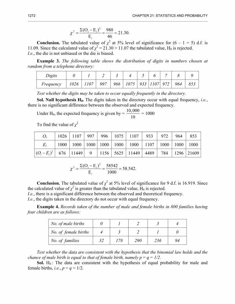
1272 CHAPTER 21: STATISTICS AND PROBABILITY ________________________________________________________________________________________________________
2
2 (O E ) 980 21.30.E 46i i
i
χ Σ −= = =
Conclusion. The tabulated value of χ2 at 5% level of significance for (6 – 1 = 5) d.f. is 11.09. Since the calculated value of χ2 = 21.30 > 11.07 the tabulated value, H0 is rejected. I.e., the die is not unbiased or the die is biased.
Example 3. The following table shows the distribution of digits in numbers chosen at random from a telephone directory:
Digits 0 1 2 3 4 5 6 7 8 9
Frequency 1026 1107 997 966 1075 933 1107 972 964 853
Test whether the digits may be taken to occur equally frequently in the directory. Sol. Null hypothesis H0. The digits taken in the directory occur with equal frequency, i.e.,
there is no significant difference between the observed and expected frequency.
Under H0, the expected frequency is given by = 10,00010
= 1000
To find the value of χ2
Oi 1026 1107 997 996 1075 1107 933 972 964 853
Ei 1000 1000 1000 1000 1000 1000 1107 1000 1000 1000 2( )i iO E− 676 11449 9 1156 5625 11449 4489 784 1296 21609
2
2 (O E ) 58542 58.542.E 1000i i
i
χ Σ −= = =
Conclusion. The tabulated value of χ2 at 5% level of significance for 9 d.f. is 16.919. Since the calculated value of χ2 is greater than the tabulated value, H0 is rejected. I.e., there is a significant difference between the observed and theoretical frequency. I.e., the digits taken in the directory do not occur with equal frequency.
Example 4. Records taken of the number of male and female births in 800 families having four children are as follows:
No. of male births 0 1 2 3 4
No. of female births 4 3 2 1 0
No. of families 32 178 290 236 94
Test whether the data are consistent with the hypothesis that the binomial law holds and the chance of male birth is equal to that of female birth, namely p = q = 1/2.
Sol. H0 : The data are consistent with the hypothesis of equal probability for male and female births, i.e., p = q = 1/2.
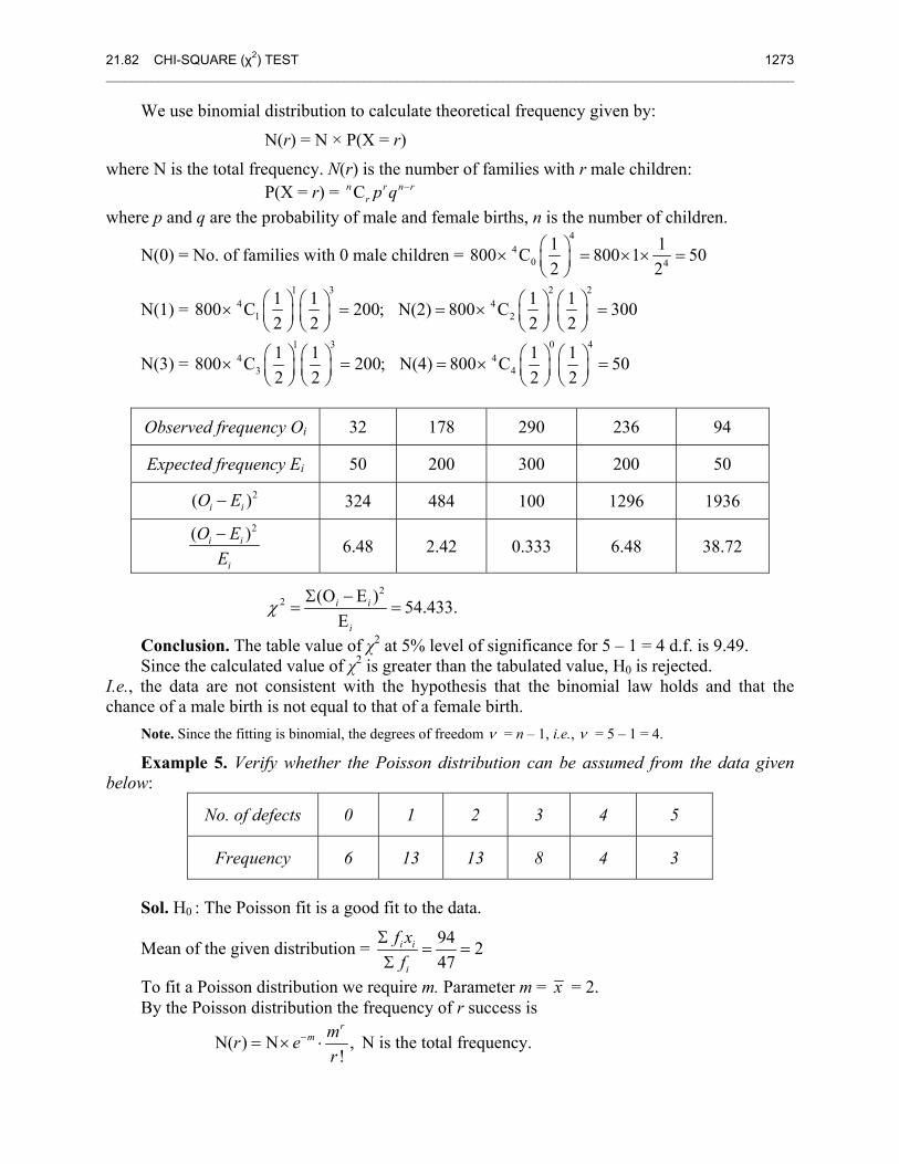
21.82 CHI-SQUARE (χ2) TEST 1273 ________________________________________________________________________________________________________
We use binomial distribution to calculate theoretical frequency given by:
N(r) = N × P(X = r)
where N is the total frequency. N(r) is the number of families with r male children: P(X = r) = Cn r n r
r p q − where p and q are the probability of male and female births, n is the number of children.
N(0) = No. of families with 0 male children = 4
40 4
1 1800 C 800 1 502 2
⎛ ⎞× = × × =⎜ ⎟⎝ ⎠
N(1) = 1 3 2 2
4 41 2
1 1 1 1800 C 200; N(2) 800 C 3002 2 2 2
⎛ ⎞ ⎛ ⎞ ⎛ ⎞ ⎛ ⎞× = = × =⎜ ⎟ ⎜ ⎟ ⎜ ⎟ ⎜ ⎟⎝ ⎠ ⎝ ⎠ ⎝ ⎠ ⎝ ⎠
N(3) = 1 3 0 4
4 43 4
1 1 1 1800 C 200; N(4) 800 C 502 2 2 2
⎛ ⎞ ⎛ ⎞ ⎛ ⎞ ⎛ ⎞× = = × =⎜ ⎟ ⎜ ⎟ ⎜ ⎟ ⎜ ⎟⎝ ⎠ ⎝ ⎠ ⎝ ⎠ ⎝ ⎠
Observed frequency Oi 32 178 290 236 94
Expected frequency Ei 50 200 300 200 50 2( )i iO E− 324 484 100 1296 1936 2( )i i
i
O EE− 6.48 2.42 0.333 6.48 38.72
2
2 (O E ) 54.433.Ei i
i
χ Σ −= =
Conclusion. The table value of χ2 at 5% level of significance for 5 – 1 = 4 d.f. is 9.49. Since the calculated value of χ2 is greater than the tabulated value, H0 is rejected.
I.e., the data are not consistent with the hypothesis that the binomial law holds and that the chance of a male birth is not equal to that of a female birth.
Note. Since the fitting is binomial, the degrees of freedom ν = n – 1, i.e., ν = 5 – 1 = 4.
Example 5. Verify whether the Poisson distribution can be assumed from the data given below:
No. of defects 0 1 2 3 4 5
Frequency 6 13 13 8 4 3
Sol. H0 : The Poisson fit is a good fit to the data.
Mean of the given distribution = 94 247
i i
i
f xf
Σ= =
Σ
To fit a Poisson distribution we require m. Parameter m = x = 2. By the Poisson distribution the frequency of r success is
N( ) N ,!
rm mr e
r−= × ⋅ N is the total frequency.
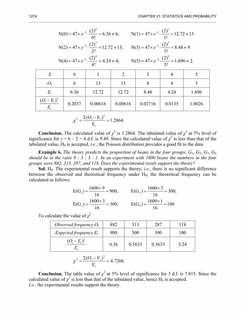
1274 CHAPTER 21: STATISTICS AND PROBABILITY ________________________________________________________________________________________________________
0 12 2
2 32 2
4 52 2
(2) (2)N(0) 47 6.36 6; N(1) 47 12.72 130! 1!
(2) (2)N(2) 47 12.72 13; N(3) 47 8.48 92! 3!
(2) (2)N(4) 47 4.24 4; N(5) 47 1.696 2.4! 5!
e e
e e
e e
− −
− −
− −
= × ⋅ = ≈ = × ⋅ = ≈
= × ⋅ = ≈ = × ⋅ = ≈
= × ⋅ = ≈ = × ⋅ = ≈
X 0 1 2 3 4 5
Oi 6 13 13 8 4 3
Ei 6.36 12.72 12.72 8.48 4.24 1.696 2( )i i
i
O EE− 0.2037 0.00616 0.00616 0.02716 0.0135 1.0026
2
2 (O E ) 1.2864.Ei i
i
χ Σ −= =
Conclusion. The calculated value of χ2 is 1.2864. The tabulated value of χ2 at 5% level of significance for γ = 6 – 2 = 4 d.f. is 9.49. Since the calculated value of χ2 is less than that of the tabulated value, H0 is accepted, i.e., the Poisson distribution provides a good fit to the data.
Example 6. The theory predicts the proportion of beans in the four groups, G1, G2, G3, G4 should be in the ratio 9 : 3 : 3 : 1. In an experiment with 1600 beans the numbers in the four groups were 882, 313, 287, and 118. Does the experimental result support the theory?
Sol. H0. The experimental result supports the theory, i.e., there is no significant difference between the observed and theoretical frequency under H0; the theoretical frequency can be calculated as follows:
1 2
3 4
1600 9 1600 3E(G ) 900; E(G ) 300;16 16
1600 3 1600 1E(G ) 300; E(G ) 10016 16
× ×= = = =
× ×= = = =
To calculate the value of χ2
Observed frequency Oi 882 313 287 118
Expected frequency Ei 900 300 300 100 2( )i i
i
O EE− 0.36 0.5633 0.5633 3.24
2
2 (O E ) 4.7266.Ei i
i
χ Σ −= =
Conclusion. The table value of χ2 at 5% level of significance for 3 d.f. is 7.815. Since the calculated value of χ2 is less than that of the tabulated value, hence H0 is accepted. I.e., the experimental results support the theory.
21.82 CHI-SQUARE (χ2) TEST 1275 ________________________________________________________________________________________________________
1. The following table gives the frequency of occupance of the digits 0, 1, . . . , 9 in the last place in four logarithms of numbers 10–99. Examine whether there is any peculiarity.
Digits : 0 1 2 3 4 5 6 7 8 9 Frequency : 6 16 15 10 12 12 3 2 9 5
2. The sales in a supermarket during a week are given below. Test the hypothesis that the sales do not depend on the day of the week, using a significance level of 0.05.
Days : Mon Tues Wed Thurs Fri Sat Sales (in $10000) : 65 54 60 56 71 84
3. A survey of 320 families with 5 children each revealed the following information:
No. of boys : 5 4 3 2 1 0 No. of girls : 0 1 2 3 4 5 No. of families : 14 56 110 88 40 12
Is this result consistent with the hypothesis that male and female births are equally probable?
4. 4 coins were tossed at a time and this operation was repeated 160 times. It is found that 4 heads occur 6 times, 3 heads occur 43 times, 2 heads occur 69 times, and one head occur 34 times. Discuss whether the coin may be regarded as unbiased.
5. Fit a Poisson distribution to the following data and the best goodness of fit:
x : 0 1 2 3 4 f : 109 65 22 3 1
6. In the accounting department of a bank, 100 accounts are selected at random and estimated for errors. The following results were obtained:
No. of errors : 0 1 2 3 4 5 6 No. of accounts : 35 40 19 2 0 2 2
Does this information verify that the errors are distributed according to the Poisson probability law?
7. In a sample analysis of examination results of 500 students, it was found that 280 students have failed, 170 have gotten C’s, 90 have gotten B’s, and the rest, A’s. Do these figures support the general belief that the above categories are in the ratio 4 : 3 : 2 : 1 respectively?
Answers 1. no 2. accepted 3. accepted 4. unbiased 5. Poisson law fits the data 6. maybe 7. yes
________________________________________________________________________________________________________
21.82.5 The χ2 Test as a Test of Independence
With the help of the χ2 test, we can find whether or not two attributes are associated. We take the null hypothesis that there is no association between the attributes under study, i.e., we assume that the two attributes are independent. If the calculated value of χ2 is less than the table value at a specified level (generally 5%) of significance, the hypothesis holds true, i.e., the attributes are independent and do not bear any association. On the other hand, if the calculated value of χ2 is greater than the table value at a specified level of significance, we say that the results of the experiment do not support the hypothesis. In other words, the attributes are associated. Thus a very useful application of the χ2 test is to investigate the relationship between trials or attributes, which can be classified into two or more categories.
TEST YOUR KNOWLEDGE
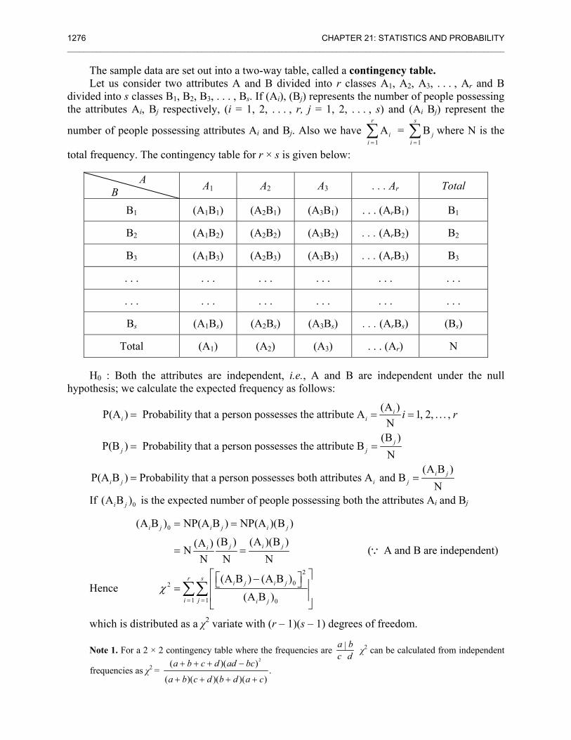
frequencies as χ2 = 2( )( )
.( )( )( )( )
a b c d ad bc
a b c d b d a c
+ + + −
+ + + +
1276 CHAPTER 21: STATISTICS AND PROBABILITY ________________________________________________________________________________________________________
The sample data are set out into a two-way table, called a contingency table. Let us consider two attributes A and B divided into r classes A1, A2, A3, . . . , Ar and B
divided into s classes B1, B2, B3, . . . , Bs. If (Ai), (Bj) represents the number of people possessing the attributes Ai, Bj respectively, (i = 1, 2, . . . , r, j = 1, 2, . . . , s) and (Ai Bj) represent the
number of people possessing attributes Ai and Bj. Also we have 1A
r
ii =∑ =
1B
s
ji =∑ where N is the
total frequency. The contingency table for r × s is given below:
A A1 A2 A3 . . . Ar Total B B1 (A1B1) (A2B1) (A3B1) . . . (ArB1) B1
B2 (A1B2) (A2B2) (A3B2) . . . (ArB2) B2
B3 (A1B3) (A2B3) (A3B3) . . . (ArB3) B3
. . . . . . . . . . . . . . . . . .
. . . . . . . . . . . . . . . . . .
Bs (A1Bs) (A2Bs) (A3Bs) . . . (ArBs) (Bs)
Total (A1) (A2) (A3) . . . (Ar) N
H0 : Both the attributes are independent, i.e., A and B are independent under the null hypothesis; we calculate the expected frequency as follows:
(A )P(A ) Probability that a person possesses the attribute A 1, 2, . . . ,N
(B )P(B ) Probability that a person possesses the attribute B
N
P(A B ) Probability that a person possesses both attributes
ii i
jj j
i j
i r= = =
= =
=(A B )
A and BNi j
i j =
If 0(A B )i j is the expected number of people possessing both the attributes Ai and Bj
Hence
0
2
02
1 1 0
(A B ) NP(A B ) NP(A )(B )
(B ) (A )(B )(A )N ( A and B are independent)N N N
(A B ) (A B )(A B )
i j i j i j
j i ji
r si j i j
i j i j
χ= =
= =
= =
⎡ ⎤⎡ ⎤−⎣ ⎦⎢ ⎥=⎢ ⎥⎣ ⎦
∑∑
∵
which is distributed as a χ2 variate with (r – 1)(s – 1) degrees of freedom.
Note 1. For a 2 × 2 contingency table where the frequencies are |a bc d χ2 can be calculated from independent
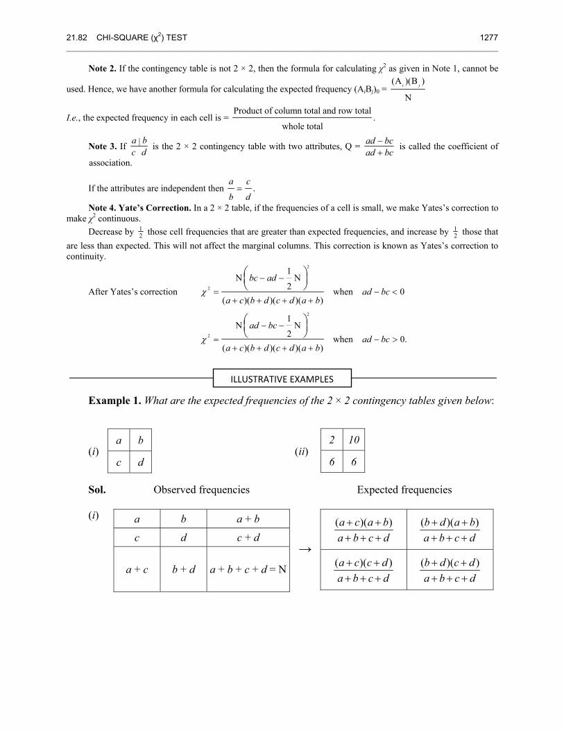
21.82 CHI-SQUARE (χ2) TEST 1277 ________________________________________________________________________________________________________
Note 2. If the contingency table is not 2 × 2, then the formula for calculating χ2 as given in Note 1, cannot be
used. Hence, we have another formula for calculating the expected frequency (AiBj)0 = (A )(B )
Ni j
I.e., the expected frequency in each cell is = Product of column total and row total
.whole total
Note 3. If |a bc d is the 2 × 2 contingency table with two attributes, Q = ad bc
ad bc−+
is called the coefficient of
If the attributes are independent then .a c
b d=
Note 4. Yate’s Correction. In a 2 × 2 table, if the frequencies of a cell is small, we make Yates’s correction to make χ2 continuous.
Decrease by 12 those cell frequencies that are greater than expected frequencies, and increase by 1
2 those that are less than expected. This will not affect the marginal columns. This correction is known as Yates’s correction to continuity.
After Yates’s correction
2
2
2
2
1N N
2 when 0( )( )( )( )
1N N
2 when 0.( )( )( )( )
bc adad bc
a c b d c d a b
ad bcad bc
a c b d c d a b
χ
χ
− −= − <
+ + + +
− −= − >
+ + + +
⎛ ⎞⎜ ⎟⎝ ⎠
⎛ ⎞⎜ ⎟⎝ ⎠
Example 1. What are the expected frequencies of the 2 × 2 contingency tables given below: (i) (ii) Sol. Observed frequencies Expected frequencies (i)
ILLUSTRATIVE EXAMPLES
association.
a b
c d
2 10
6 6
a b a + b
c d c + d
a + c b + d a + b + c + d = N
( )( )a c a ba b c d+ ++ + +
( )( )b d a ba b c d+ ++ + +
( )( )a c c da b c d+ ++ + +
( )( )b d c da b c d+ ++ + +
→
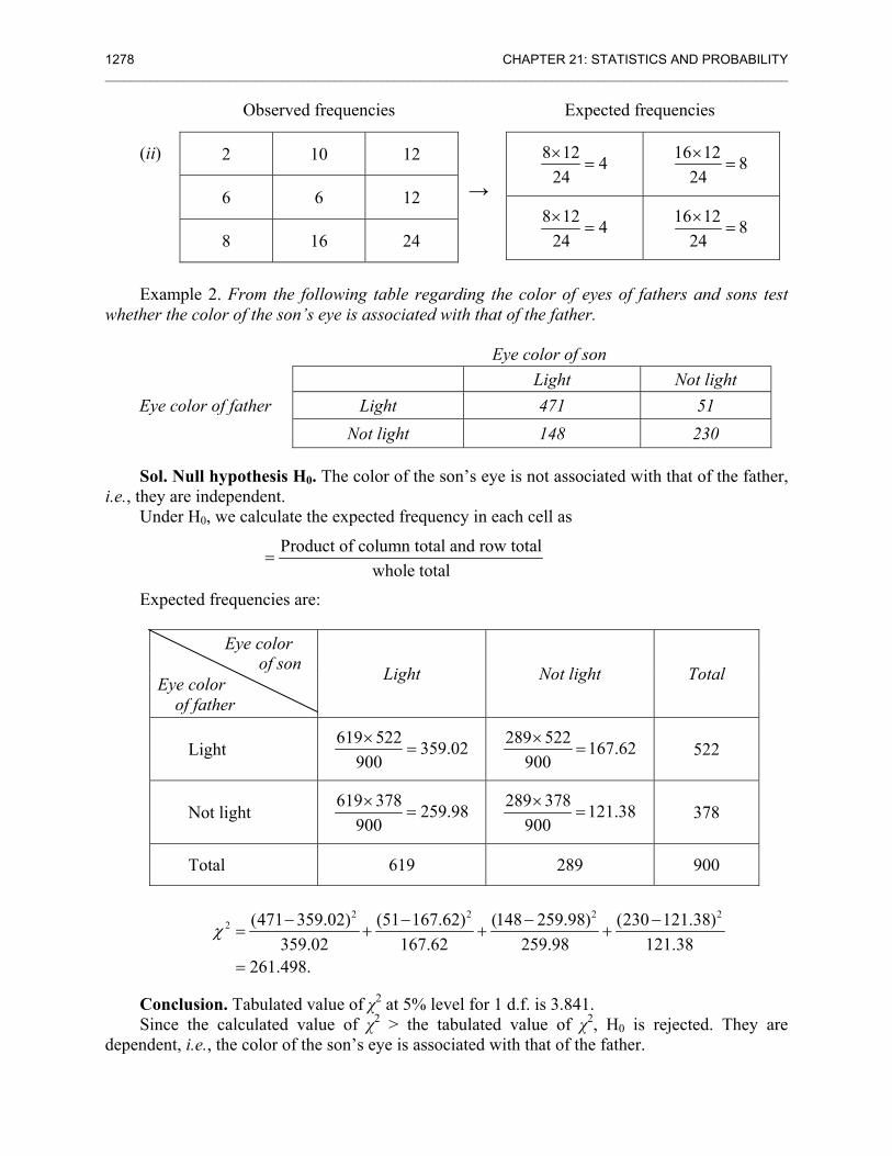
1278 CHAPTER 21: STATISTICS AND PROBABILITY ________________________________________________________________________________________________________
Observed frequencies Expected frequencies (ii) Example 2. From the following table regarding the color of eyes of fathers and sons test
whether the color of the son’s eye is associated with that of the father.
Eye color of son Light Not light Eye color of father Light 471 51 Not light 148 230
Sol. Null hypothesis H0. The color of the son’s eye is not associated with that of the father, i.e., they are independent.
Under H0, we calculate the expected frequency in each cell as
Product of column total and row totalwhole total
=
Expected frequencies are:
Eye color of son Light Not light Total Eye color
of father
Light 619 522 359.02
900×
= 289 522 167.62900×
= 522
Not light 619 378 259.98
900×
= 289 378 121.38900×
= 378
Total 619 289 900
2 2 2 2
2 (471 359.02) (51 167.62) (148 259.98) (230 121.38)359.02 167.62 259.98 121.38
261.498.
χ − − − −= + + +
=
Conclusion. Tabulated value of χ2 at 5% level for 1 d.f. is 3.841. Since the calculated value of χ2 > the tabulated value of χ2, H0 is rejected. They are
dependent, i.e., the color of the son’s eye is associated with that of the father.
2 10 12
6 6 12
8 16 24
8 12 424×
= 16 12 824×
=
8 12 424×
= 16 12 824×
=
→
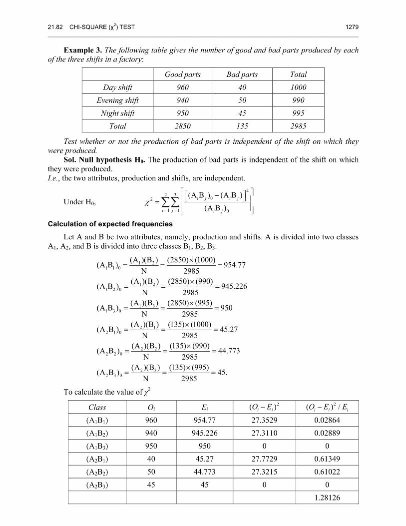
21.82 CHI-SQUARE (χ2) TEST 1279 ________________________________________________________________________________________________________
Example 3. The following table gives the number of good and bad parts produced by each of the three shifts in a factory:
Good parts Bad parts Total Day shift 960 40 1000
Evening shift 940 50 990 Night shift 950 45 995
Total 2850 135 2985
Test whether or not the production of bad parts is independent of the shift on which they were produced.
Sol. Null hypothesis H0. The production of bad parts is independent of the shift on which they were produced. I.e., the two attributes, production and shifts, are independent.
Under H0, 2
2 302
1 1 0
(A B ) (A B )(A B )
i j i j
i j i j
χ= =
⎡ ⎤⎡ ⎤−⎣ ⎦⎢ ⎥=⎢ ⎥⎣ ⎦
∑∑
Calculation of expected frequencies
Let A and B be two attributes, namely, production and shifts. A is divided into two classes A1, A2, and B is divided into three classes B1, B2, B3.
1 21 1 0
1 21 2 0
1 31 3 0
2 12 1 0
2 22 2 0
(A )(B ) (2850) (1000)(A B ) 954.77N 2985
(A )(B ) (2850) (990)(A B ) 945.226N 2985
(A )(B ) (2850) (995)(A B ) 950N 2985
(A )(B ) (135) (1000)(A B ) 45.27N 2985
(A )(B ) (135) (990)(A B ) 44.7N 2985
×= = =
×= = =
×= = =
×= = =
×= = =
2 32 3 0
73
(A )(B ) (135) (995)(A B ) 45.N 2985
×= = =
To calculate the value of χ2
Class Oi Ei 2( )i iO E− 2( ) /i i iO E E−
(A1B1) 960 954.77 27.3529 0.02864 (A1B2) 940 945.226 27.3110 0.02889 (A1B3) 950 950 0 0 (A2B1) 40 45.27 27.7729 0.61349 (A2B2) 50 44.773 27.3215 0.61022 (A2B3) 45 45 0 0
1.28126
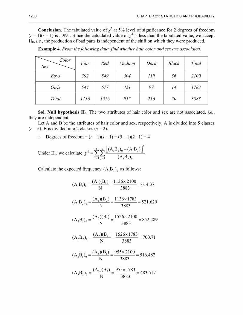
1280 CHAPTER 21: STATISTICS AND PROBABILITY ________________________________________________________________________________________________________
Conclusion. The tabulated value of χ2 at 5% level of significance for 2 degrees of freedom (r – 1)(s – 1) is 5.991. Since the calculated value of χ2 is less than the tabulated value, we accept H0, i.e., the production of bad parts is independent of the shift on which they were produced.
Example 4. From the following data, find whether hair color and sex are associated.
Color Fair Red Medium Dark Black Total
Sex
Boys 592 849 504 119 36 2100
Girls 544 677 451 97 14 1783
Total 1136 1526 955 216 50 3883
Sol. Null hypothesis H0. The two attributes of hair color and sex are not associated, i.e., they are independent.
Let A and B be the attributes of hair color and sex, respectively. A is divided into 5 classes (r = 5). B is divided into 2 classes (s = 2).
∴ Degrees of freedom = (r – 1)(s – 1) = (5 – 1)(2– 1) = 4
Under H0, we calculate 2
5 202
1 1 0
(A B ) (A B )(A B )
i j i j
i j i j
χ= =
⎡ ⎤−⎣ ⎦=∑∑
Calculate the expected frequency 0(A B )i j as follows:
1 11 1 0
1 21 2 0
2 12 1 0
2 22 2 0
3 13 1 0
3 2 0
(A )(B ) 1136 2100(A B ) 614.37N 3883
(A )(B ) 1136 1783(A B ) 521.629N 3883
(A )(B ) 1526 2100(A B ) 852.289N 3883
(A )(B ) 1526 1783(A B ) 700.71N 3883
(A )(B ) 955 2100(A B ) 516.482N 3883
(A B )
×= = =
×= = =
×= = =
×= = =
×= = =
= 3 2(A )(B ) 955 1783 483.517N 3883
×= =
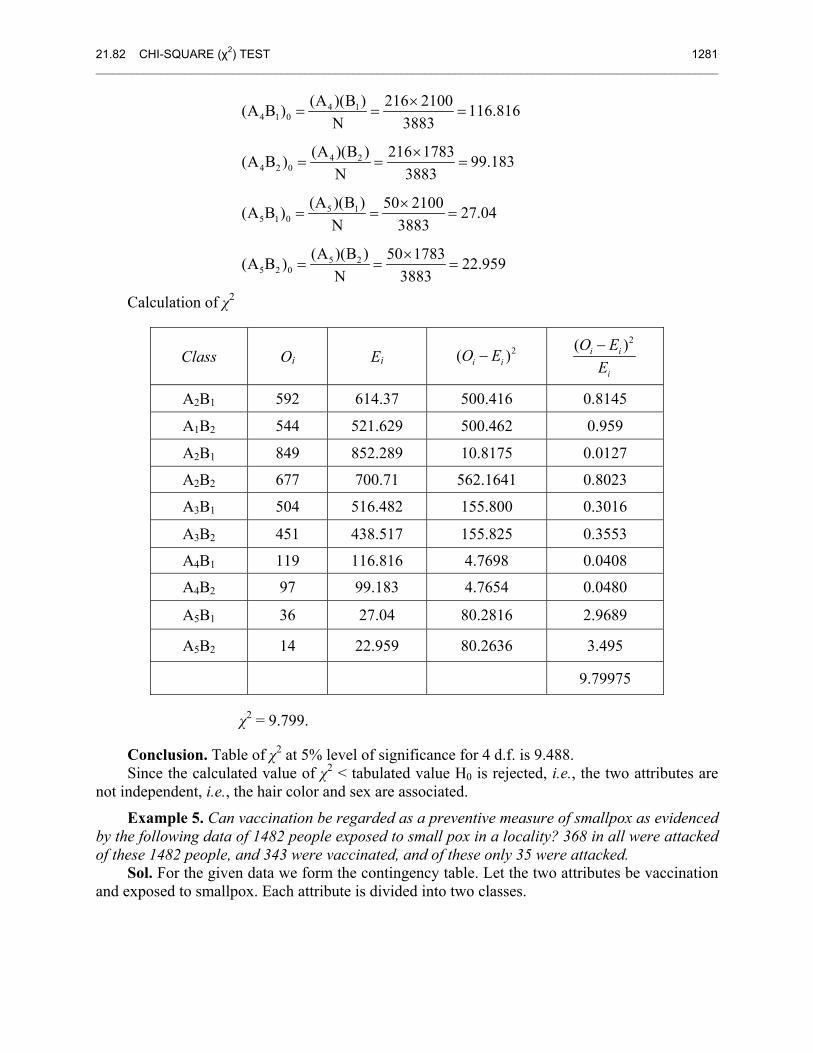
21.82 CHI-SQUARE (χ2) TEST 1281 ________________________________________________________________________________________________________
4 14 1 0
4 24 2 0
5 15 1 0
5 25 2 0
(A )(B ) 216 2100(A B ) 116.816N 3883
(A )(B ) 216 1783(A B ) 99.183N 3883
(A )(B ) 50 2100(A B ) 27.04N 3883
(A )(B ) 50 1783(A B ) 22.959N 3883
×= = =
×= = =
×= = =
×= = =
Calculation of χ2
Class Oi Ei 2( )i iO E−
2( )i i
i
O EE−
A2B1 592 614.37 500.416 0.8145
A1B2 544 521.629 500.462 0.959
A2B1 849 852.289 10.8175 0.0127
A2B2 677 700.71 562.1641 0.8023
A3B1 504 516.482 155.800 0.3016
A3B2 451 438.517 155.825 0.3553
A4B1 119 116.816 4.7698 0.0408
A4B2 97 99.183 4.7654 0.0480
A5B1 36 27.04 80.2816 2.9689
A5B2 14 22.959 80.2636 3.495
9.79975
χ2 = 9.799.
Conclusion. Table of χ2 at 5% level of significance for 4 d.f. is 9.488. Since the calculated value of χ2 < tabulated value H0 is rejected, i.e., the two attributes are
not independent, i.e., the hair color and sex are associated.
Example 5. Can vaccination be regarded as a preventive measure of smallpox as evidenced by the following data of 1482 people exposed to small pox in a locality? 368 in all were attacked of these 1482 people, and 343 were vaccinated, and of these only 35 were attacked.
Sol. For the given data we form the contingency table. Let the two attributes be vaccination and exposed to smallpox. Each attribute is divided into two classes.
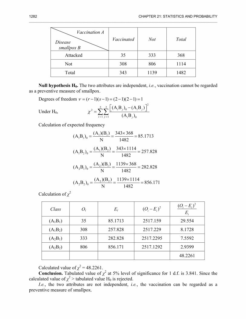
1282 CHAPTER 21: STATISTICS AND PROBABILITY ________________________________________________________________________________________________________
Vaccination A Vaccinated Not Total Disease
smallpox B Attacked 35 333 368
Not 308 806 1114
Total 343 1139 1482 Null hypothesis H0. The two attributes are independent, i.e., vaccination cannot be regarded
as a preventive measure of smallpox.
Degrees of freedom ( 1)( 1) (2 1)(2 1) 1r sν = − − = − − =
Under H0, 2
2 202
1 1 0
(A B ) (A B )(A B )
i j i j
i j i j
χ= =
⎡ ⎤−⎣ ⎦=∑∑
Calculation of expected frequency
1 11 1 0
1 21 2 0
2 12 1 0
2 22 2 0
(A )(B ) 343 368(A B ) 85.1713N 1482
(A )(B ) 343 1114(A B ) 257.828N 1482
(A )(B ) 1139 368(A B ) 282.828N 1482
(A )(B ) 1139 1114(A B ) 856.171N 1482
×= = =
×= = =
×= = =
×= = =
Calculation of χ2
Class Oi Ei 2( )i iO E−
2( )i i
i
O EE−
(A1B1) 35 85.1713 2517.159 29.554
(A1B2) 308 257.828 2517.229 8.1728
(A2B1) 333 282.828 2517.2295 7.5592
(A2B2) 806 856.171 2517.1292 2.9399
48.2261
Calculated value of χ2 = 48.2261. Conclusion. Tabulated value of χ2 at 5% level of significance for 1 d.f. is 3.841. Since the
calculated value of χ2 > tabulated value H0 is rejected. I.e., the two attributes are not independent, i.e., the vaccination can be regarded as a
preventive measure of smallpox.
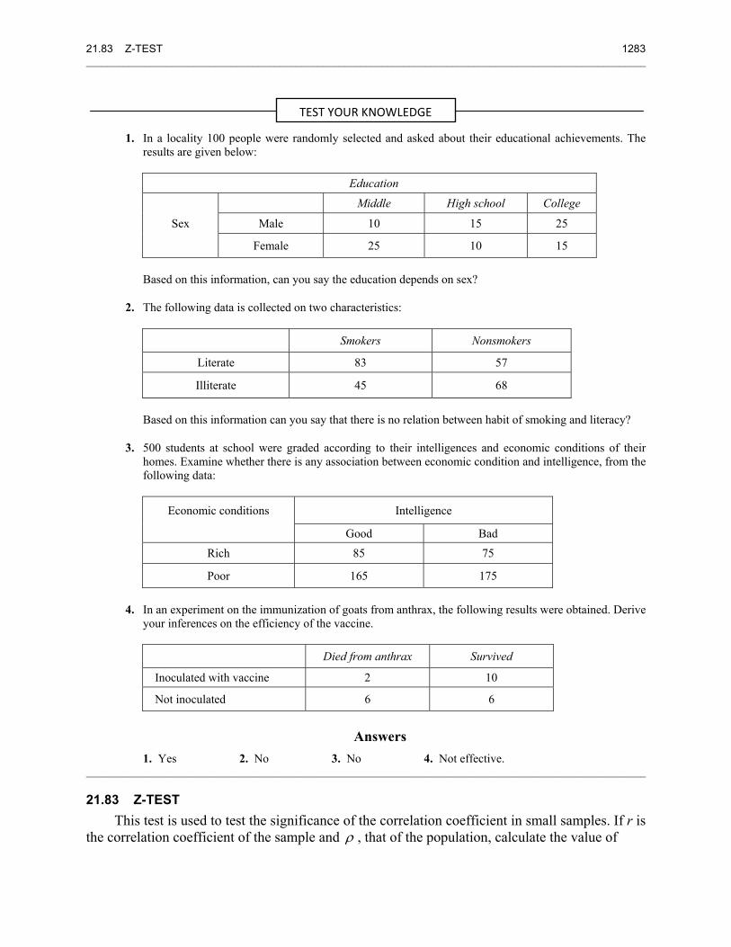
21.83 Z-TEST 1283 ________________________________________________________________________________________________________
1. In a locality 100 people were randomly selected and asked about their educational achievements. The results are given below:
Education
Middle High school College
Sex Male 10 15 25
Female 25 10 15
Based on this information, can you say the education depends on sex?
2. The following data is collected on two characteristics:
Smokers Nonsmokers
Literate 83 57
Illiterate 45 68
Based on this information can you say that there is no relation between habit of smoking and literacy?
3. 500 students at school were graded according to their intelligences and economic conditions of their homes. Examine whether there is any association between economic condition and intelligence, from the following data:
Economic conditions Intelligence
Good Bad
Rich 85 75
Poor 165 175
4. In an experiment on the immunization of goats from anthrax, the following results were obtained. Derive your inferences on the efficiency of the vaccine.
Died from anthrax Survived
Inoculated with vaccine 2 10
Not inoculated 6 6
Answers
1. Yes 2. No 3. No 4. Not effective. ________________________________________________________________________________________________________
21.83 Z-TEST This test is used to test the significance of the correlation coefficient in small samples. If r is
the correlation coefficient of the sample and ρ , that of the population, calculate the value of
TEST YOUR KNOWLEDGE
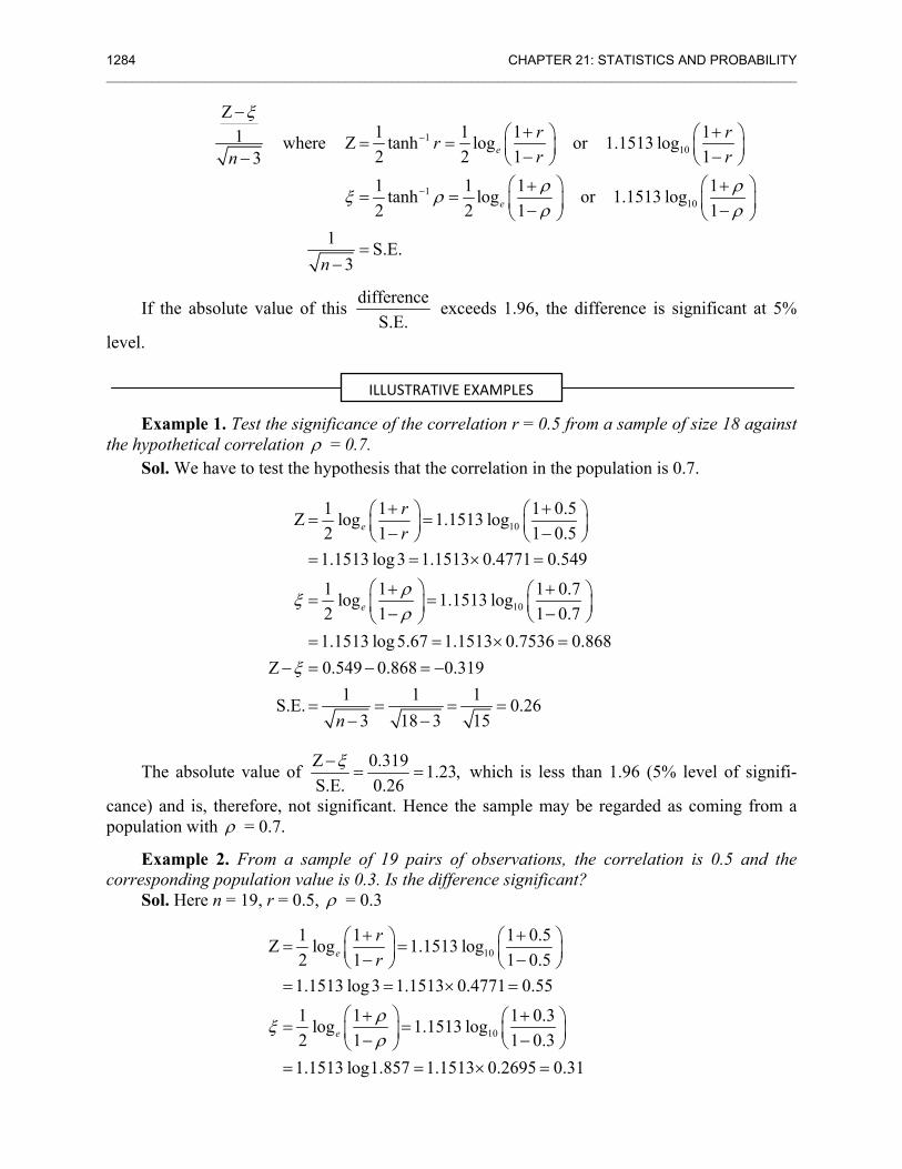
1284 CHAPTER 21: STATISTICS AND PROBABILITY ________________________________________________________________________________________________________
110
110
Z1 1 1 11 where Z tanh log or 1.1513 log2 2 1 131 1 1 1tanh log or 1.1513 log2 2 1 1
1 S.E.3
e
e
r rrr rn
n
ξ
ρ ρξ ρρ ρ
−
−
−+ +⎛ ⎞ ⎛ ⎞= = ⎜ ⎟ ⎜ ⎟− −− ⎝ ⎠ ⎝ ⎠
⎛ ⎞ ⎛ ⎞+ += = ⎜ ⎟ ⎜ ⎟− −⎝ ⎠ ⎝ ⎠
=−
If the absolute value of this differenceS.E.
exceeds 1.96, the difference is significant at 5%
level.
Example 1. Test the significance of the correlation r = 0.5 from a sample of size 18 against the hypothetical correlation ρ = 0.7.
Sol. We have to test the hypothesis that the correlation in the population is 0.7.
10
10
1 1 1 0.5Z log 1.1513 log2 1 1 0.51.1513 log3 1.1513 0.4771 0.549
1 1 1 0.7log 1.1513 log2 1 1 0.71.1513 log5.67 1.1513 0.7536 0.868
Z 0.549 0.868 0.3191 1 1S.E.
3 18 3
e
e
rr
n
ρξρ
ξ
+ +⎛ ⎞ ⎛ ⎞= =⎜ ⎟ ⎜ ⎟− −⎝ ⎠ ⎝ ⎠= = × =
⎛ ⎞+ +⎛ ⎞= = ⎜ ⎟⎜ ⎟− −⎝ ⎠⎝ ⎠= = × =
− = − = −
= = =− −
0.2615
=
The absolute value of Z 0.319 1.23,S.E. 0.26
ξ−= = which is less than 1.96 (5% level of signifi-
cance) and is, therefore, not significant. Hence the sample may be regarded as coming from a population with ρ = 0.7.
Example 2. From a sample of 19 pairs of observations, the correlation is 0.5 and the corresponding population value is 0.3. Is the difference significant?
Sol. Here n = 19, r = 0.5, ρ = 0.3
10
10
1 1 1 0.5Z log 1.1513 log2 1 1 0.51.1513 log3 1.1513 0.4771 0.55
1 1 1 0.3log 1.1513 log2 1 1 0.31.1513 log1.857 1.1513 0.2695 0.31
e
e
rr
ρξρ
+ +⎛ ⎞ ⎛ ⎞= =⎜ ⎟ ⎜ ⎟− −⎝ ⎠ ⎝ ⎠= = × =
⎛ ⎞+ +⎛ ⎞= = ⎜ ⎟⎜ ⎟− −⎝ ⎠⎝ ⎠= = × =
ILLUSTRATIVE EXAMPLES
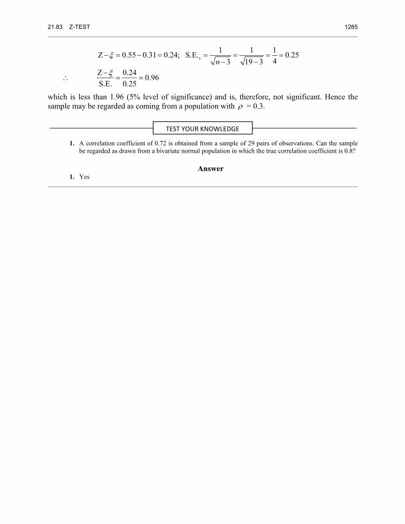
21.83 Z-TEST 1285 ________________________________________________________________________________________________________
∴
1 1 1Z 0.55 0.31 0.24; S.E. 0.2543 19 3
Z 0.24 0.96S.E. 0.25
x nξ
ξ
− = − = = = = =− −
−= =
which is less than 1.96 (5% level of significance) and is, therefore, not significant. Hence the sample may be regarded as coming from a population with ρ = 0.3.
1. A correlation coefficient of 0.72 is obtained from a sample of 29 pairs of observations. Can the sample be regarded as drawn from a bivariate normal population in which the true correlation coefficient is 0.8?
Answer
1. Yes ________________________________________________________________________________________________________
TEST YOUR KNOWLEDGE