Embed Size (px)
Citation preview
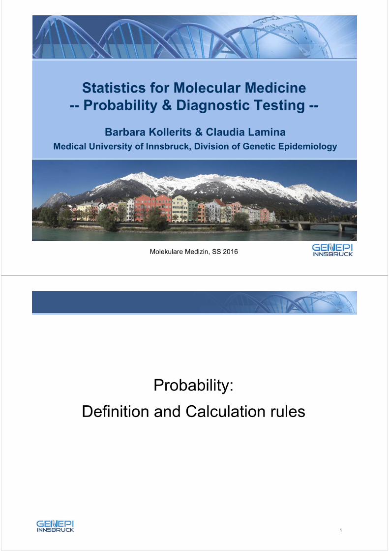
Statistics for Molecular Medicine -- Probability & Diagnostic Testing --
Barbara Kollerits & Claudia LaminaMedical University of Innsbruck, Division of Genetic Epidemiology
Molekulare Medizin, SS 2016
2
Probability:
Definition and Calculation rules
1
3
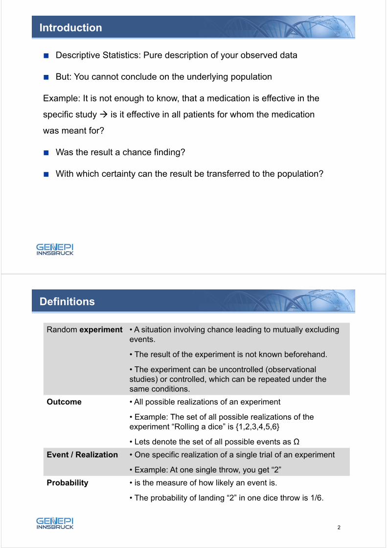
Descriptive Statistics: Pure description of your observed data
But: You cannot conclude on the underlying population
Example: It is not enough to know, that a medication is effective in the
specific study is it effective in all patients for whom the medication
was meant for?
Was the result a chance finding?
With which certainty can the result be transferred to the population?
Introduction
Random experiment • A situation involving chance leading to mutually excluding events.
• The result of the experiment is not known beforehand.
• The experiment can be uncontrolled (observational studies) or controlled, which can be repeated under the same conditions.
Outcome • All possible realizations of an experiment
• Example: The set of all possible realizations of the experiment “Rolling a dice” is 1,2,3,4,5,6
• Lets denote the set of all possible events as Ω
Event / Realization • One specific realization of a single trial of an experiment
• Example: At one single throw, you get “2”
Probability • is the measure of how likely an event is.
• The probability of landing “2” in one dice throw is 1/6.
Definitions
2
5
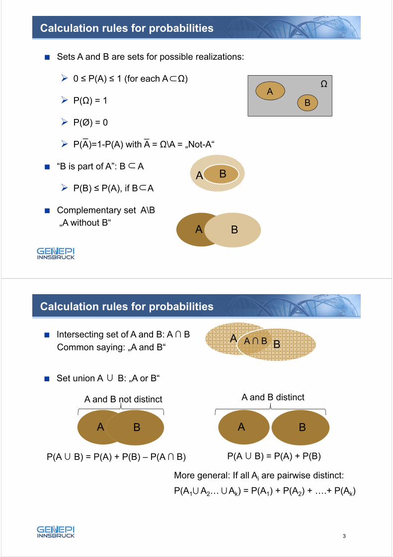
Sets A and B are sets for possible realizations:
0 ≤ P(A) ≤ 1 (for each A Ω)
P(Ω) = 1
P(Ø) = 0
P(A)=1-P(A) with A = Ω\A = „Not-A“
“B is part of A”: B A
P(B) ≤ P(A), if B A
Complementary set A\B
Calculation rules for probabilities
AB
Ω
∩
BA
∩_ _
„A without B“A B
∩
6
Intersecting set of A and B: A ∩ B
Set union A B: „A or B“
Calculation rules for probabilities
A BA ∩ B
∩
A B
Common saying: „A and B“
A B
A and B not distinct A and B distinct
P(A B) = P(A) + P(B) – P(A ∩ B)
∩
P(A B) = P(A) + P(B)
∩
More general: If all Ai are pairwise distinct:
P(A1 A2… Ak) = P(A1) + P(A2) + ….+ P(Ak)
∩
∩
3
“Counting rule” for Probability:
“Counting rule” for Odds:
Definition of Odds:
Example: Experiment = Tossing a coin once
P(„Head“) = 0.5
Odds („Head“) = 1:1
7
Calculation rules for probabilities
The number of ways event A can occurThe total number of possible outcomes
P(A)=
7The number of ways event A can occur P(A)=
The number of ways event A can not occur
P(A) Odds(A)=1-P(A)
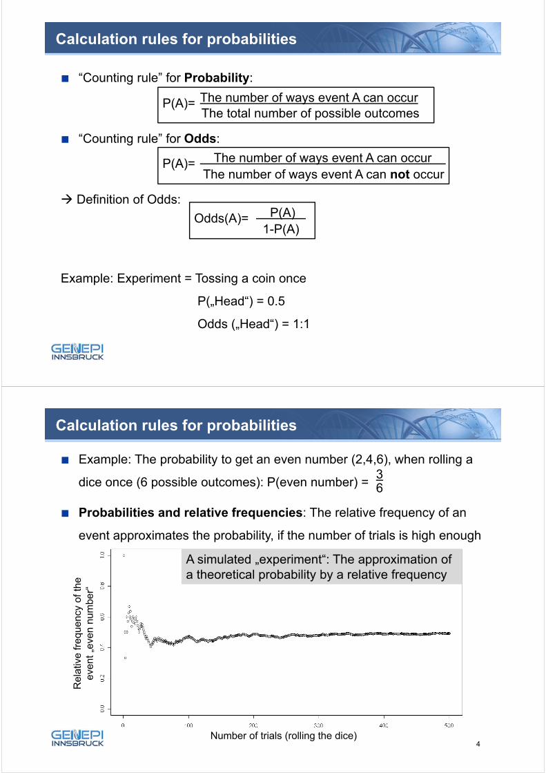
Example: The probability to get an even number (2,4,6), when rolling a
dice once (6 possible outcomes): P(even number) =
Probabilities and relative frequencies: The relative frequency of an
event approximates the probability, if the number of trials is high enough
Calculation rules for probabilities
36
Number of trials (rolling the dice)
Rel
ativ
e fr
eque
ncy
ofth
eev
ent
„eve
nnu
mbe
r“
A simulated „experiment“: The approximation ofa theoretical probability by a relative frequency
4
9
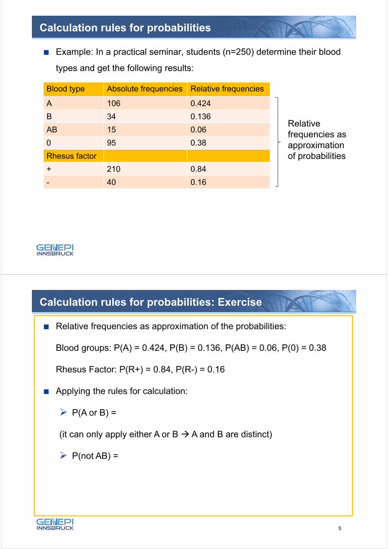
Example: In a practical seminar, students (n=250) determine their blood
types and get the following results:
Calculation rules for probabilities
Blood type Absolute frequencies Relative frequencies
A 106 0.424
B 34 0.136
AB 15 0.06
0 95 0.38
Rhesus factor
+ 210 0.84
- 40 0.16
Relative frequencies asapproximationof probabilities
10
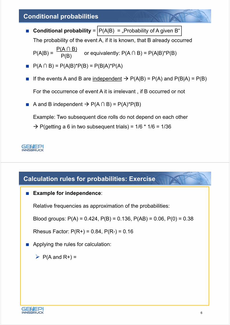
Relative frequencies as approximation of the probabilities:
Blood groups: P(A) = 0.424, P(B) = 0.136, P(AB) = 0.06, P(0) = 0.38
Rhesus Factor: P(R+) = 0.84, P(R-) = 0.16
Applying the rules for calculation:
P(A or B) =
(it can only apply either A or B A and B are distinct)
P(not AB) =
Calculation rules for probabilities: Exercise
5
11
Conditional probability = P(A|B) = „Probability of A given B“
The probability of the event A, if it is known, that B already occurred
P(A|B) = or equivalently: P(A ∩ B) = P(A|B)*P(B)
P(A ∩ B) = P(A|B)*P(B) = P(B|A)*P(A)
If the events A and B are independent P(A|B) = P(A) and P(B|A) = P(B)
For the occurrence of event A it is irrelevant , if B occurred or not
A and B independent P(A ∩ B) = P(A)*P(B)
Example: Two subsequent dice rolls do not depend on each other
P(getting a 6 in two subsequent trials) = 1/6 * 1/6 = 1/36
Conditional probabilities
P(A ∩ B)P(B)
12
Example for independence:
Relative frequencies as approximation of the probabilities:
Blood groups: P(A) = 0.424, P(B) = 0.136, P(AB) = 0.06, P(0) = 0.38
Rhesus Factor: P(R+) = 0.84, P(R-) = 0.16
Applying the rules for calculation:
P(A and R+) =
Calculation rules for probabilities: Exercise
6
13
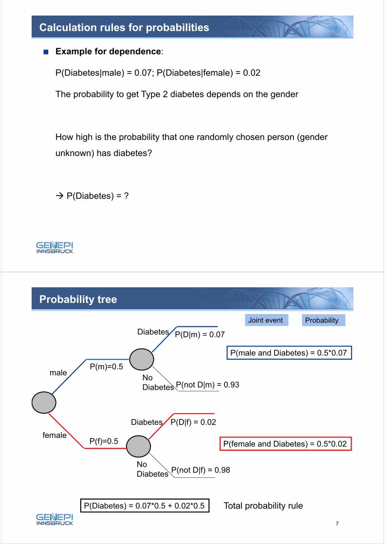
Example for dependence:
P(Diabetes|male) = 0.07; P(Diabetes|female) = 0.02
The probability to get Type 2 diabetes depends on the gender
How high is the probability that one randomly chosen person (gender
unknown) has diabetes?
P(Diabetes) = ?
Calculation rules for probabilities
14
Joint event Probability
Probability tree
male
female
P(m)=0.5
P(f)=0.5
Diabetes P(D|m) = 0.07
NoDiabetes P(not D|m) = 0.93
Diabetes
NoDiabetes P(not D|f) = 0.98
P(D|f) = 0.02
P(male and Diabetes) = 0.5*0.07
P(female and Diabetes) = 0.5*0.02
P(Diabetes) = 0.07*0.5 + 0.02*0.5 Total probability rule
7
15
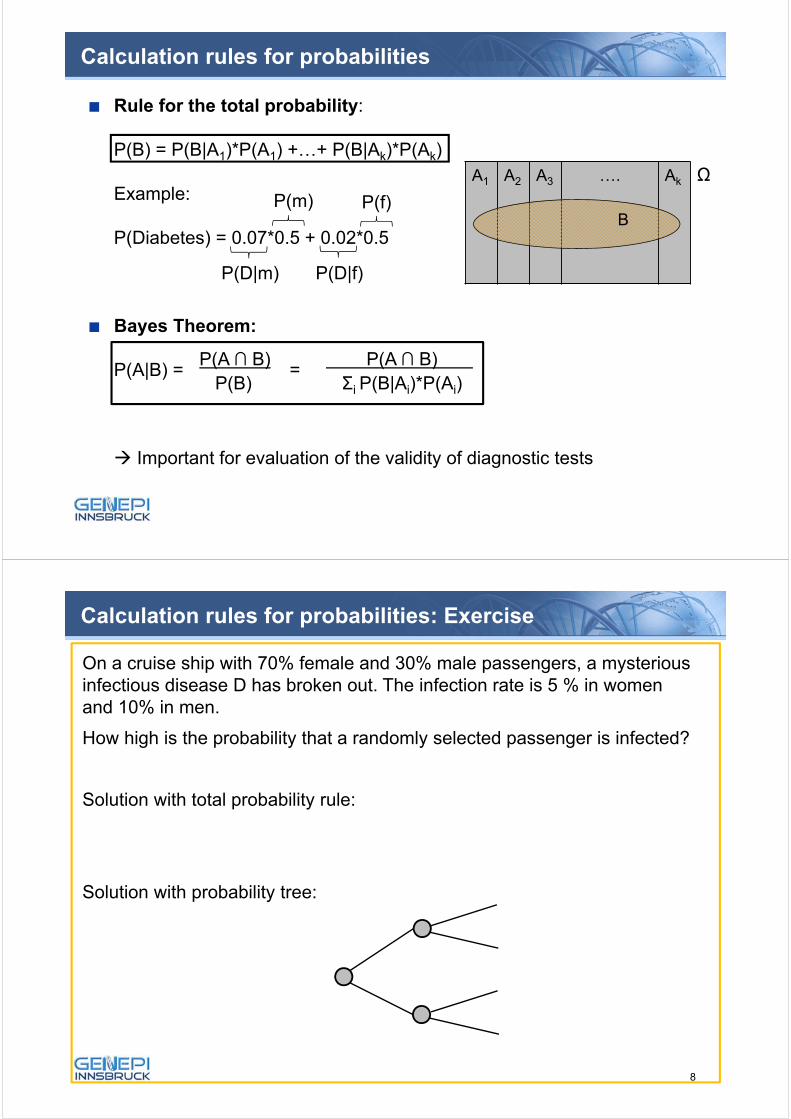
Rule for the total probability:
P(B) = P(B|A1)*P(A1) +…+ P(B|Ak)*P(Ak)
Example:
P(Diabetes) = 0.07*0.5 + 0.02*0.5
Bayes Theorem:
P(A|B) = =
Important for evaluation of the validity of diagnostic tests
Calculation rules for probabilities
ΩA1 A2 A3 …. Ak
B
P(A ∩ B)P(B)
P(A ∩ B) Σi P(B|Ai)*P(Ai)
P(m) P(f)
P(D|f)P(D|m)
Calculation rules for probabilities: Exercise
On a cruise ship with 70% female and 30% male passengers, a mysteriousinfectious disease D has broken out. The infection rate is 5 % in womenand 10% in men.
How high is the probability that a randomly selected passenger is infected?
Solution with total probability rule:
Solution with probability tree:
8
Diagnostic Testing
Intention:
To find a marker / specific test, that discriminates patients into diseased or
non-diseased
How accurate is a test? Can it detect all currently diseased and exclude all non-diseased (e.g. Elisa test, Westernblot, PCR etc.). How likely is it, that a person is actually diseased/non-diseased, if the test is positive/negative?
Make predictions for individuals, who will get the disease in the future
Example 1: Predict the progression of a chronic disease using a biomarker
Example 2: Predict the probability to get a disease in the future based on genetic variants
Example: Ideal situation – perfect test
9
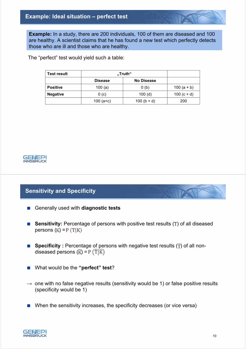
Example: In a study, there are 200 individuals, 100 of them are diseased and 100 are healthy. A scientist claims that he has found a new test which perfectly detects those who are ill and those who are healthy.
The “perfect” test would yield such a table:
Example: Ideal situation – perfect test
19
Test result „Truth“
Disease No Disease
Positive 100 (a) 0 (b) 100 (a + b)
Negative 0 (c) 100 (d) 100 (c + d)
100 (a+c) 100 (b + d) 200
Sensitivity and Specificity
Generally used with diagnostic tests
Sensitivity: Percentage of persons with positive test results ( ) of all diseased persons ( ) =
Specificity : Percentage of persons with negative test results ( ) of all non-diseased persons ( ) =
What would be the “perfect” test?
→ one with no false negative results (sensitivity would be 1) or false positive results (specificity would be 1)
When the sensitivity increases, the specificity decreases (or vice versa)
10
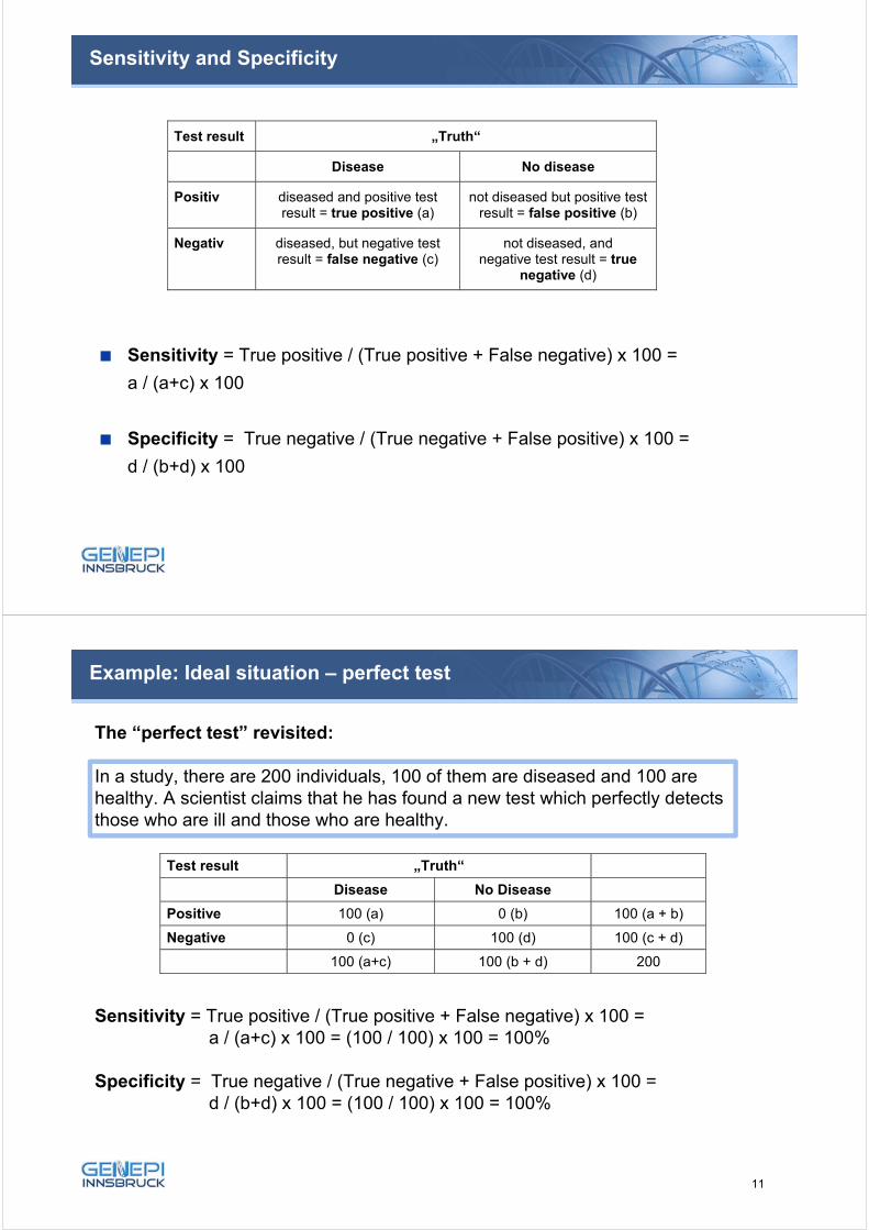
Sensitivity and Specificity
Sensitivity = True positive / (True positive + False negative) x 100 =
a / (a+c) x 100
Specificity = True negative / (True negative + False positive) x 100 =
d / (b+d) x 100
Test result „Truth“
Disease No disease
Positiv diseased and positive test result = true positive (a)
not diseased but positive test result = false positive (b)
Negativ diseased, but negative test result = false negative (c)
not diseased, and negative test result = true
negative (d)
Example: Ideal situation – perfect test
22
Test result „Truth“
Disease No Disease
Positive 100 (a) 0 (b) 100 (a + b)
Negative 0 (c) 100 (d) 100 (c + d)
100 (a+c) 100 (b + d) 200
The “perfect test” revisited:
In a study, there are 200 individuals, 100 of them are diseased and 100 are healthy. A scientist claims that he has found a new test which perfectly detects those who are ill and those who are healthy.
Sensitivity = True positive / (True positive + False negative) x 100 = a / (a+c) x 100 = (100 / 100) x 100 = 100%
Specificity = True negative / (True negative + False positive) x 100 = d / (b+d) x 100 = (100 / 100) x 100 = 100%
11
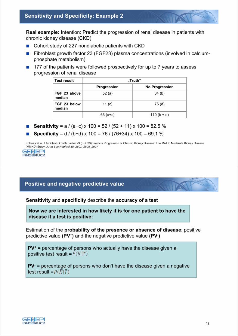
Sensitivity and Specificity: Example 2
Real example: Intention: Predict the progression of renal disease in patients with chronic kidney disease (CKD)
Cohort study of 227 nondiabetic patients with CKD
Fibroblast growth factor 23 (FGF23) plasma concentrations (involved in calcium-phosphate metabolism)
177 of the patients were followed prospectively for up to 7 years to assess progression of renal disease
Sensitivity = a / (a+c) x 100 = 52 / (52 + 11) x 100 = 82.5 %
Specificity = d / (b+d) x 100 = 76 / (76+34) x 100 = 69.1 %
23Kollerits et al. Fibroblast Growth Factor 23 (FGF23) Predicts Progression of Chronic Kidney Disease: The Mild to Moderate Kidney Disease (MMKD) Study. J Am Soc Nephrol 18: 2601–2608, 2007
Test result „Truth“
Progression No Progression
FGF 23 above median
52 (a) 34 (b)
FGF 23 below median
11 (c) 76 (d)
63 (a+c) 110 (b + d)
Positive and negative predictive value
Sensitivity and specificity describe the accuracy of a test
Estimation of the probability of the presence or absence of disease: positive predictive value (PV+) and the negative predictive value (PV-)
Now we are interested in how likely it is for one patient to have the disease if a test is positive:
PV+ = percentage of persons who actually have the disease given a positive test result =
PV- = percentage of persons who don’t have the disease given a negative test result =
12
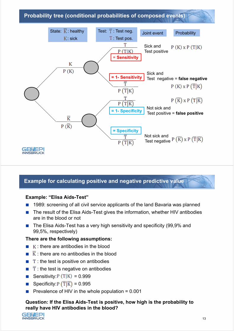
Probability tree (conditional probabilities of composed events)
25
Sick and Test positive
Sick and Test negative = false negative
Not sick and Test positive = false positive
Not sick and Test negative
State: : healthy
: sick
Test: : Test neg.
: Test pos.Joint event Probability
= Sensitivity
= 1- Sensitivity
= Specificity
= 1- Specificity
Example for calculating positive and negative predictive value
Example: “Elisa Aids-Test”
1989: screening of all civil service applicants of the land Bavaria was planned
The result of the Elisa Aids-Test gives the information, whether HIV antibodies are in the blood or not
The Elisa Aids-Test has a very high sensitivity and specificity (99,9% and 99,5%, respectively)
There are the following assumptions:
: there are antibodies in the blood
: there are no antibodies in the blood
: the test is positive on antibodies
: the test is negative on antibodies
Sensitivity: = 0.999
Specificity: = 0.995
Prevalence of HIV in the whole population = 0.001
Question: If the Elisa Aids-Test is positive, how high is the probability to really have HIV antibodies in the blood?
13
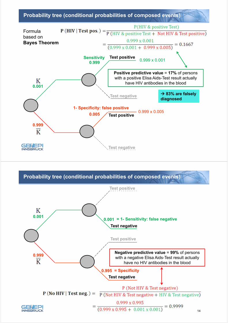
Probability tree (conditional probabilities of composed events)
0.001
No HIV
HIV
Test positive
Test positive
0.999
Test negative
Test negative
0.999 x 0.001
0.999
0.0050.999 x 0.005
Positive predictive value = 17% of persons with a positive Elisa Aids-Test result actually
have HIV antibodies in the blood
83% are falsely diagnosed
Formula based on Bayes Theorem:
Sensitivity
1- Specificity: false positive
Test positive
Probability tree (conditional probabilities of composed events)
0.001
No HIV
HIV
Test positive
Test positive
Test negative
Test negative
0.999
0.995
0.001
Negative predictive value = 99% of persons with a negative Elisa Aids-Test result actually
have no HIV antibodies in the blood
= 1- Sensitivity: false negative
= Specificity
14
Relation between positive and negative predictive value
29
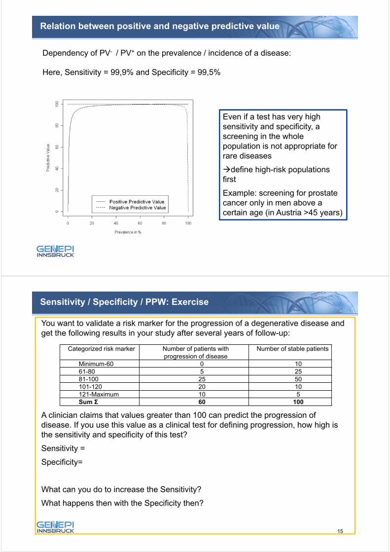
Dependency of PV- / PV+ on the prevalence / incidence of a disease:
Here, Sensitivity = 99,9% and Specificity = 99,5%
Even if a test has very high sensitivity and specificity, a screening in the whole population is not appropriate for rare diseases
define high-risk populations first
Example: screening for prostate cancer only in men above a certain age (in Austria >45 years)
You want to validate a risk marker for the progression of a degenerative disease and get the following results in your study after several years of follow-up:
A clinician claims that values greater than 100 can predict the progression ofdisease. If you use this value as a clinical test for defining progression, how high is the sensitivity and specificity of this test?
Sensitivity =
Specificity=
What can you do to increase the Sensitivity?
What happens then with the Specificity then?
Categorized risk marker Number of patients withprogression of disease
Number of stable patients
Minimum-60 0 1061-80 5 2581-100 25 50101-120 20 10121-Maximum 10 5Sum Σ 60 100
Sensitivity / Specificity / PPW: Exercise
15
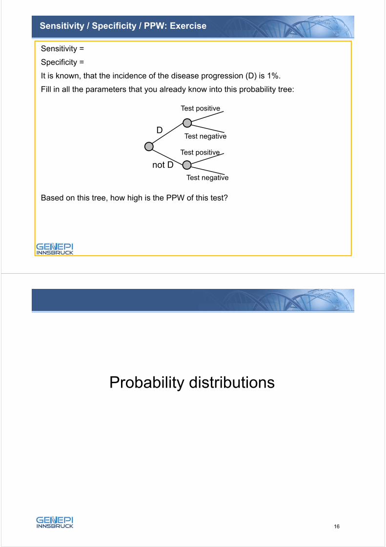
Sensitivity =
Specificity =
It is known, that the incidence of the disease progression (D) is 1%.
Fill in all the parameters that you already know into this probability tree:
Based on this tree, how high is the PPW of this test?
Sensitivity / Specificity / PPW: Exercise
D
not D
Test positive
Test negative
Test positive
Test negative
32
Probability distributions
16
33
Random variable X: The values of a random variable X are the
outcomes of a random experiment. A number is assigned to all possible
realizations of a random experiment.
Realization of a random variable X in an experiment: xi
Discrete random variable: Qualitative variables, like gender, disease
status etc.
Continuous random variable: Qualitative variable like age, cholesterol
levels etc.
Definitions
Why are gender, disease status, age etc. „random“?
They are outcomes of the random experiment„Drawing one person from the population“
34
A random variable is discrete, if it can only take a finite number of
realizations
To each realization, a specific probability can be assigned:
f(x) = P(X = xi) = pi Probability function
Distribution function :
F(x) = P(X ≤ x) Probability that X takes the values of x or smaller than x
A distribution function is increasing monotonically and is the sum of the
probabilities of all realizations ≤ x
Discrete random variables
17
35
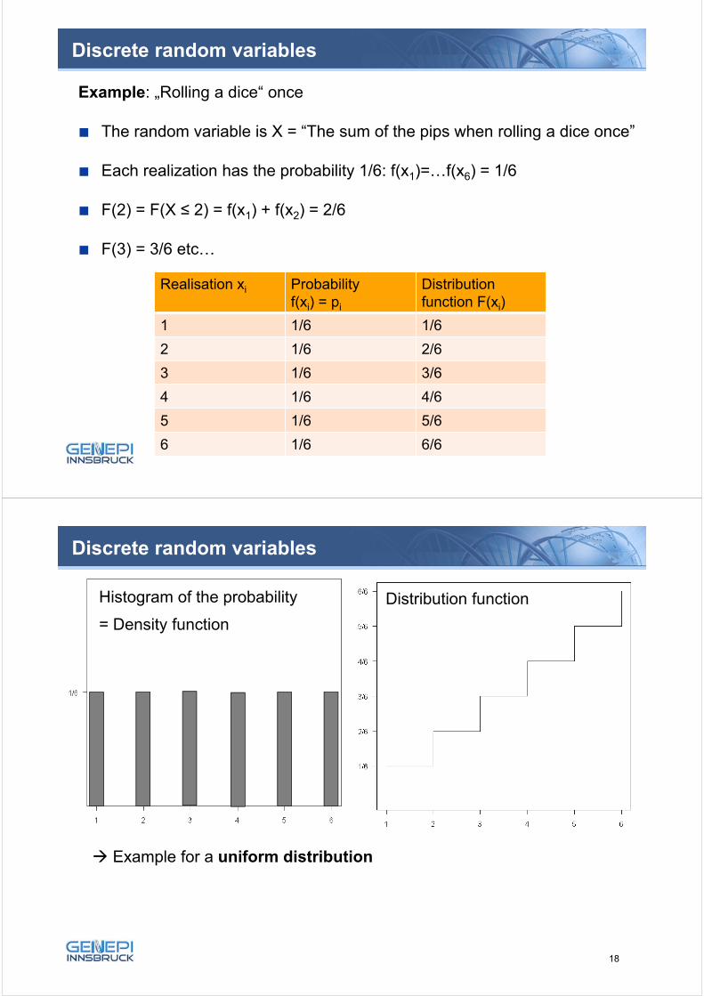
Example: „Rolling a dice“ once
The random variable is X = “The sum of the pips when rolling a dice once”
Each realization has the probability 1/6: f(x1)=…f(x6) = 1/6
F(2) = F(X ≤ 2) = f(x1) + f(x2) = 2/6
F(3) = 3/6 etc…
Discrete random variables
Realisation xi Probabilityf(xi) = pi
Distribution function F(xi)
1 1/6 1/6
2 1/6 2/6
3 1/6 3/6
4 1/6 4/6
5 1/6 5/6
6 1/6 6/6
36
Discrete random variables
Example for a uniform distribution
Histogram of the probability
= Density function
Distribution function
18
37
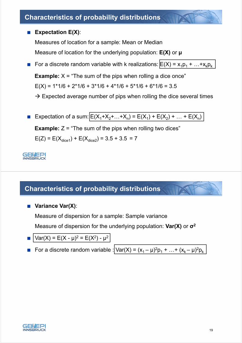
Characteristics of probability distributions
Expectation E(X):
Measures of location for a sample: Mean or Median
Measure of location for the underlying population: E(X) or μ
For a discrete random variable with k realizations: E(X) = x1p1 + …+xkpk
Example: X = “The sum of the pips when rolling a dice once”
E(X) = 1*1/6 + 2*1/6 + 3*1/6 + 4*1/6 + 5*1/6 + 6*1/6 = 3.5
Expected average number of pips when rolling the dice several times
Expectation of a sum: E(X1+X2+…+Xn) = E(X1) + E(X2) + … + E(Xn)
Example: Z = “The sum of the pips when rolling two dices”
E(Z) = E(Xdice1) + E(Xdice2) = 3.5 + 3.5 = 7
38
Characteristics of probability distributions
Variance Var(X):
Measure of dispersion for a sample: Sample variance
Measure of dispersion for the underlying population: Var(X) or σ2
Var(X) = E(X - μ)2 = E(X2) - μ2
For a discrete random variable : Var(X) = (x1 – μ)2p1 + …+ (xk – μ)2pk
19
39
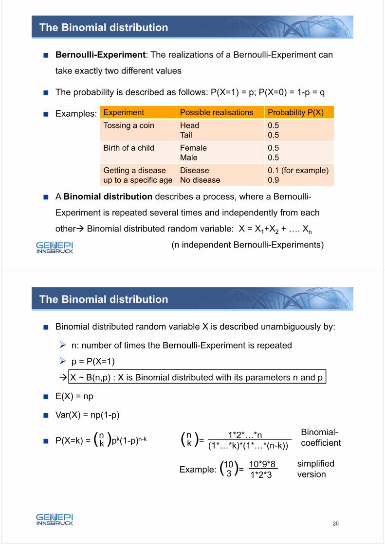
The Binomial distribution
Bernoulli-Experiment: The realizations of a Bernoulli-Experiment can
take exactly two different values
The probability is described as follows: P(X=1) = p; P(X=0) = 1-p = q
Examples:
A Binomial distribution describes a process, where a Bernoulli-
Experiment is repeated several times and independently from each
other Binomial distributed random variable: X = X1+X2 + …. Xn
(n independent Bernoulli-Experiments)
Experiment Possible realisations Probability P(X)
Tossing a coin HeadTail
0.50.5
Birth of a child FemaleMale
0.50.5
Getting a diseaseup to a specific age
DiseaseNo disease
0.1 (for example)0.9
40
The Binomial distribution
Binomial distributed random variable X is described unambiguously by:
n: number of times the Bernoulli-Experiment is repeated
p = P(X=1)
X ~ B(n,p) : X is Binomial distributed with its parameters n and p
E(X) = np
Var(X) = np(1-p)
P(X=k) = ( )pk(1-p)n-k ( )= nk
nk
1*2*…*n (1*…*k)*(1*…*(n-k))
Binomial-coefficient
Example: ( )=103
10*9*8 1*2*3
simplifiedversion
20
41
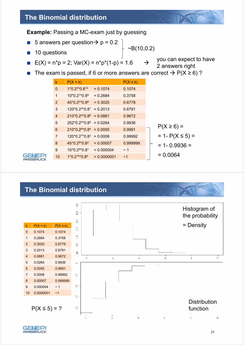
The Binomial distribution
Example: Passing a MC-exam just by guessing
5 answers per question p = 0.2
10 questions
E(X) = n*p = 2; Var(X) = n*p*(1-p) = 1.6
The exam is passed, if 6 or more answers are correct P(X ≥ 6) ?
~B(10,0.2)
you can expect to have 2 answers right
k P(X = k) P(X ≤ k)
0 1*0.20*0.810 = 0.1074 0.1074
1 10*0.21*0.89 = 0.2684 0.3758
2 45*0.22*0.88 = 0.3020 0.6778
3 120*0.23*0.87 = 0.2013 0.8791
4 210*0.24*0.86 = 0.0881 0.9672
5 252*0.25*0.85 = 0.0264 0.9936
6 210*0.26*0.84 = 0.0055 0.9991
7 120*0.27*0.83 = 0.0008 0.99992
8 45*0.28*0.82 = 0.00007 0.999999
9 10*0.29*0.81 = 0.000004 ~ 1
10 1*0.210*0.80 = 0.0000001 ~1
P(X ≥ 6) =
= 1- P(X ≤ 5) =
= 1- 0.9936 =
= 0.0064
42
The Binomial distribution
Histogram ofthe probability
= Density
Distribution function
k P(X = k) P(X ≤ k)
0 0.1074 0.1074
1 0.2684 0.3758
2 0.3020 0.6778
3 0.2013 0.8791
4 0.0881 0.9672
5 0.0264 0.9936
6 0.0055 0.9991
7 0.0008 0.99992
8 0.00007 0.999999
9 0.000004 ~ 1
10 0.0000001 ~1
Distribution functionP(X ≤ 5) = ?
21
43
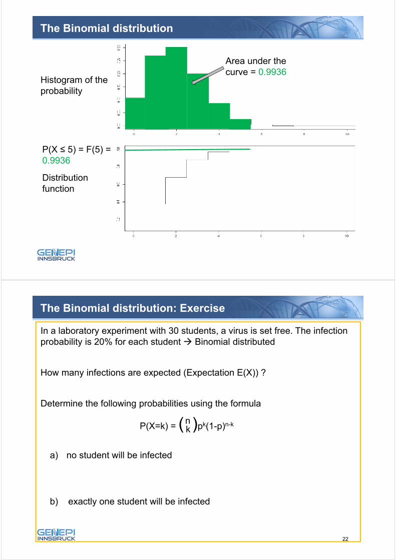
The Binomial distribution
Histogram of theprobability
Distribution function
P(X ≤ 5) = F(5) = 0.9936
Area under thecurve = 0.9936
The Binomial distribution: Exercise
In a laboratory experiment with 30 students, a virus is set free. The infectionprobability is 20% for each student Binomial distributed
How many infections are expected (Expectation E(X)) ?
Determine the following probabilities using the formula
P(X=k) = ( )pk(1-p)n-k
a) no student will be infected
b) exactly one student will be infected
nk
22
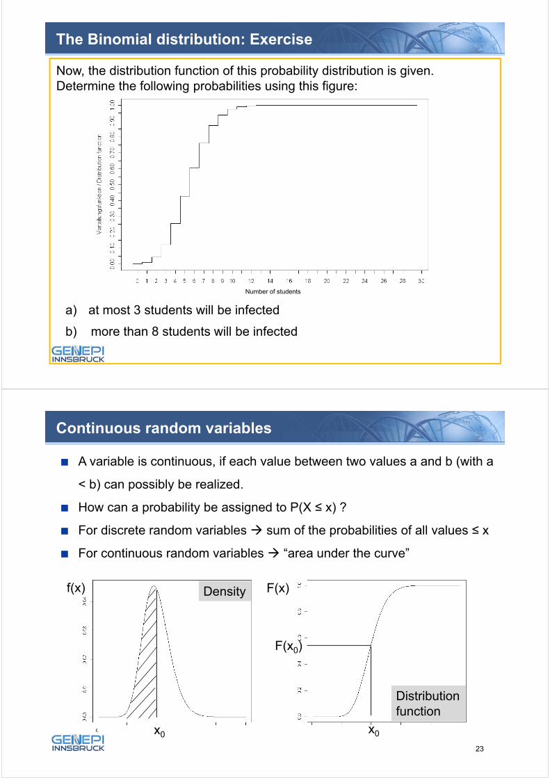
The Binomial distribution: Exercise
Now, the distribution function of this probability distribution is given. Determine the following probabilities using this figure:
a) at most 3 students will be infected
b) more than 8 students will be infected
Number of students
46
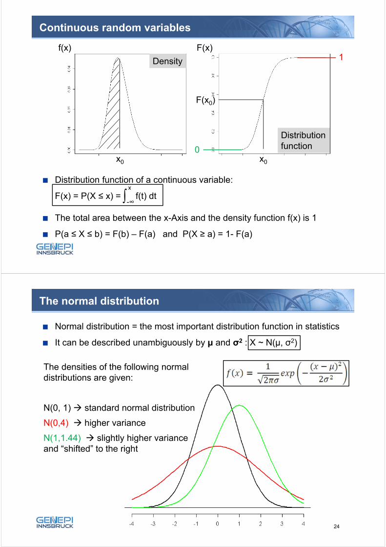
Continuous random variables
A variable is continuous, if each value between two values a and b (with a
< b) can possibly be realized.
How can a probability be assigned to P(X ≤ x) ?
For discrete random variables sum of the probabilities of all values ≤ x
For continuous random variables “area under the curve”
f(x) F(x)
x0 x0
F(x0)
Density
Distribution function
23
47
Continuous random variables
Distribution function of a continuous variable:
F(x) = P(X ≤ x) = f(t) dt
f(x) F(x)
x0 x0
F(x0)
Density
x
∫-∞ The total area between the x-Axis and the density function f(x) is 1
P(a ≤ X ≤ b) = F(b) – F(a) and P(X ≥ a) = 1- F(a)
Distribution function
1
0
48
The normal distribution
Normal distribution = the most important distribution function in statistics
It can be described unambiguously by μ and σ2 : X ~ N(μ, σ2)
The densities of the following normal distributions are given:
N(0, 1) standard normal distribution
N(0,4) higher variance
N(1,1.44) slightly higher variance and “shifted” to the right
24
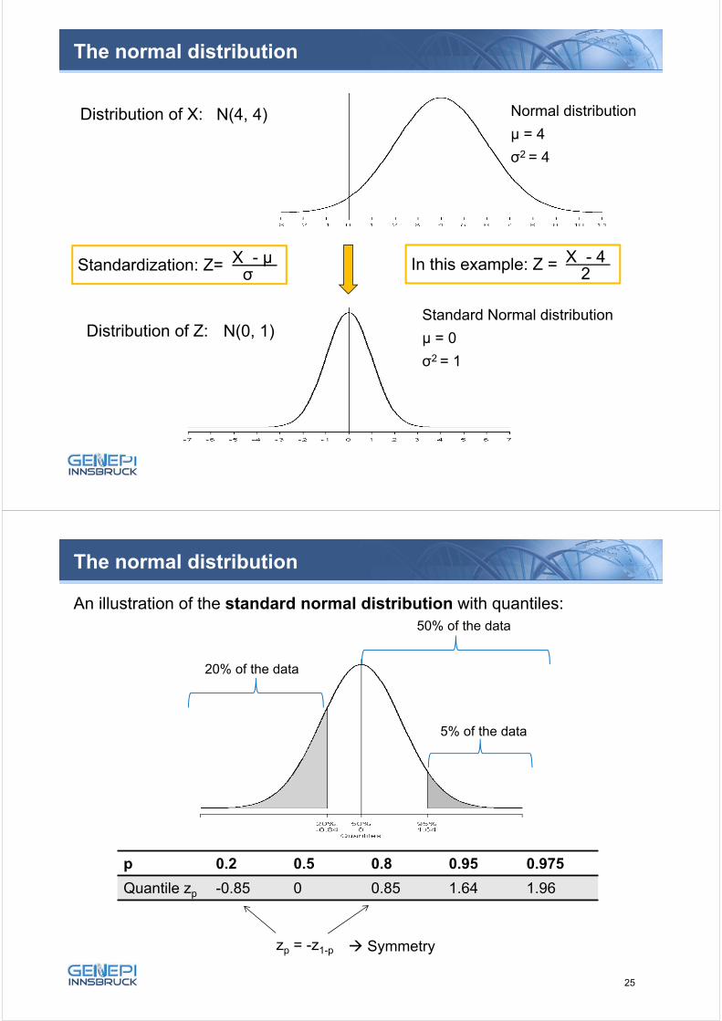
Normal distribution
μ = 4
σ2 = 4
Standard Normal distribution
μ = 0
σ2 = 1
Standardization: Z=
The normal distribution
N(4, 4)
N(0, 1)
X - μσ
In this example: Z = X - 42
Distribution of X:
Distribution of Z:
An illustration of the standard normal distribution with quantiles:
20% of the data
50% of the data
5% of the data
p 0.2 0.5 0.8 0.95 0.975
Quantile zp -0.85 0 0.85 1.64 1.96
zp = -z1-p
The normal distribution
Symmetry
25
51
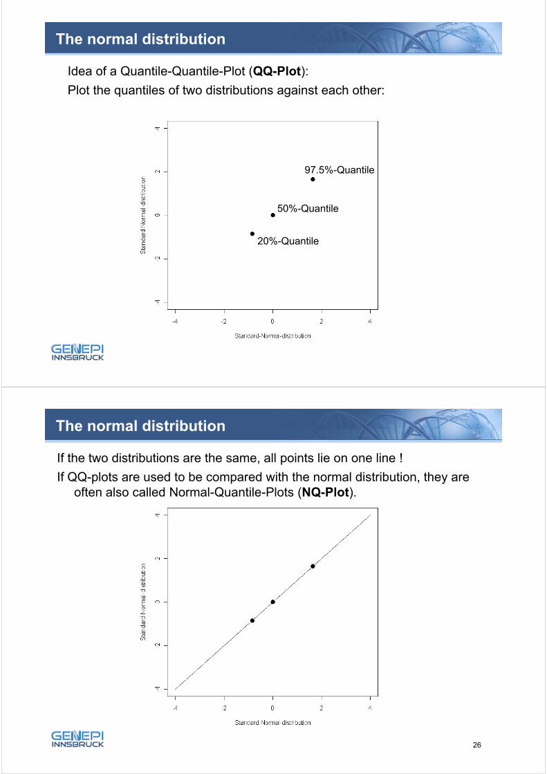
Idea of a Quantile-Quantile-Plot (QQ-Plot):
Plot the quantiles of two distributions against each other:
20%-Quantile
50%-Quantile
97.5%-Quantile
The normal distribution
If the two distributions are the same, all points lie on one line !
If QQ-plots are used to be compared with the normal distribution, they areoften also called Normal-Quantile-Plots (NQ-Plot).
50%-Quantile
The normal distribution
26
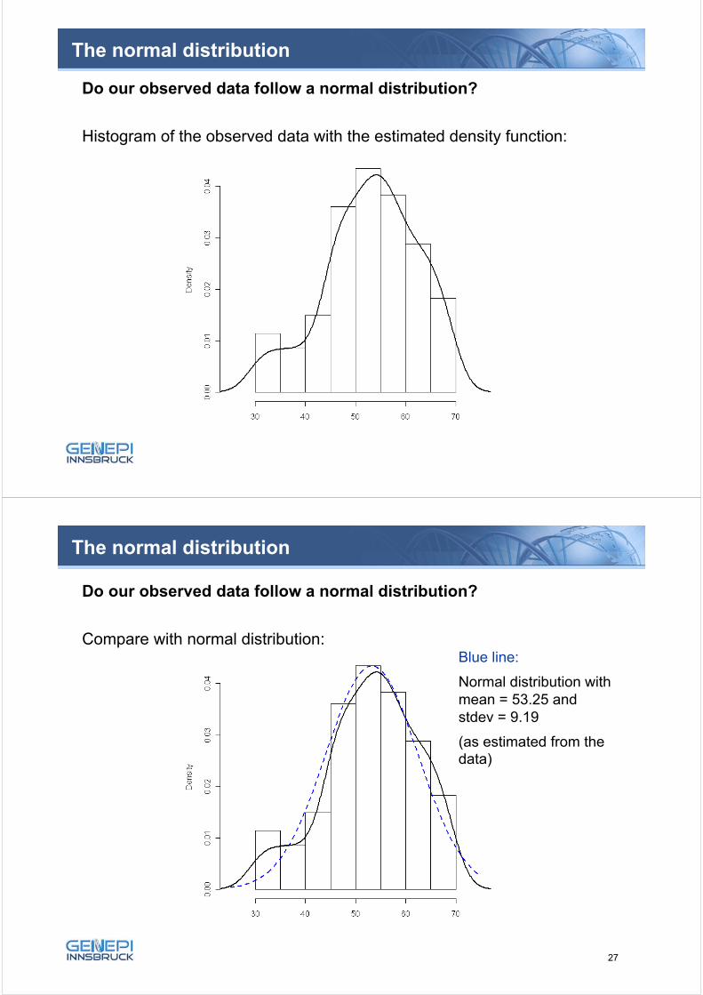
Do our observed data follow a normal distribution?
Histogram of the observed data with the estimated density function:
The normal distribution
Do our observed data follow a normal distribution?
Compare with normal distribution:Blue line:
Normal distribution withmean = 53.25 and stdev = 9.19
(as estimated from the data)
The normal distribution
27
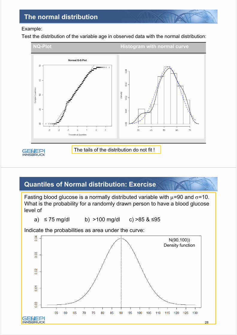
NQ-Plot Histogram with normal curve
Example:
Test the distribution of the variable age in observed data with the normal distribution:
The tails of the distribution do not fit !
The normal distribution
Quantiles of Normal distribution: Exercise
Fasting blood glucose is a normally distributed variable with =90 and =10. What is the probability for a randomly drawn person to have a blood glucoselevel of
a) ≤ 75 mg/dl b) >100 mg/dl c) >85 & ≤95
Indicate the probabilities as area under the curve:
N(90,100)) Density function
28
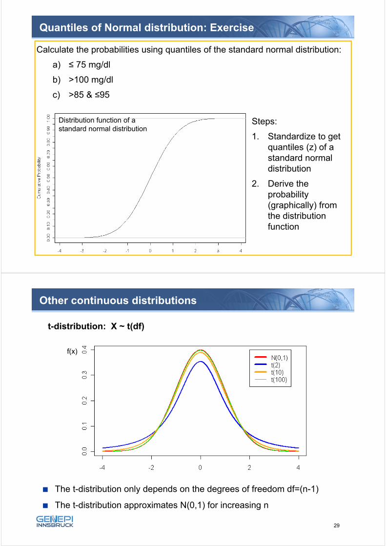
Quantiles of Normal distribution: Exercise
Calculate the probabilities using quantiles of the standard normal distribution:
a) ≤ 75 mg/dl
b) >100 mg/dl
c) >85 & ≤95
Distribution function of a standard normal distribution
Steps:
1. Standardize to getquantiles (z) of a standard normal distribution
2. Derive theprobability(graphically) fromthe distributionfunction
Other continuous distributions
t-distribution: X ~ t(df)
The t-distribution only depends on the degrees of freedom df=(n-1)
The t-distribution approximates N(0,1) for increasing n
f(x)
29
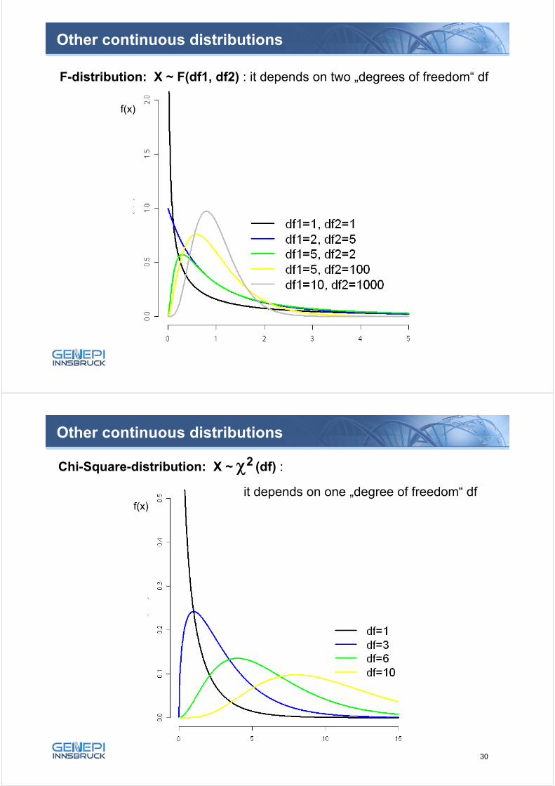
Other continuous distributions
F-distribution: X ~ F(df1, df2) : it depends on two „degrees of freedom“ df
f(x)
Other continuous distributions
Chi-Square-distribution: X ~ 2 (df) :
it depends on one „degree of freedom“ dff(x)
30
Point and Confidence Estimates
Point and confidence estimates
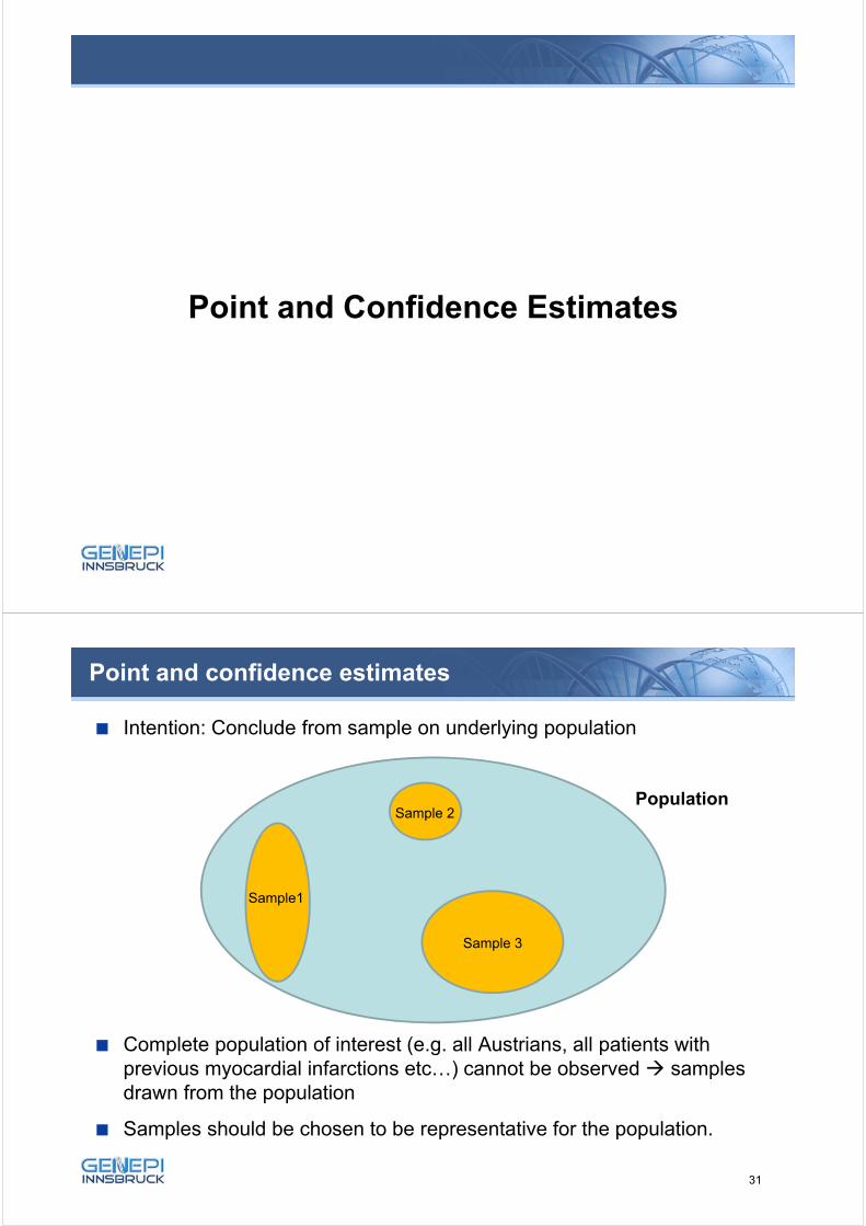
Intention: Conclude from sample on underlying population
Complete population of interest (e.g. all Austrians, all patients with previous myocardial infarctions etc…) cannot be observed samples drawn from the population
Samples should be chosen to be representative for the population.
Sample1
Sample 3
Sample 2Population
31
Point and confidence estimates
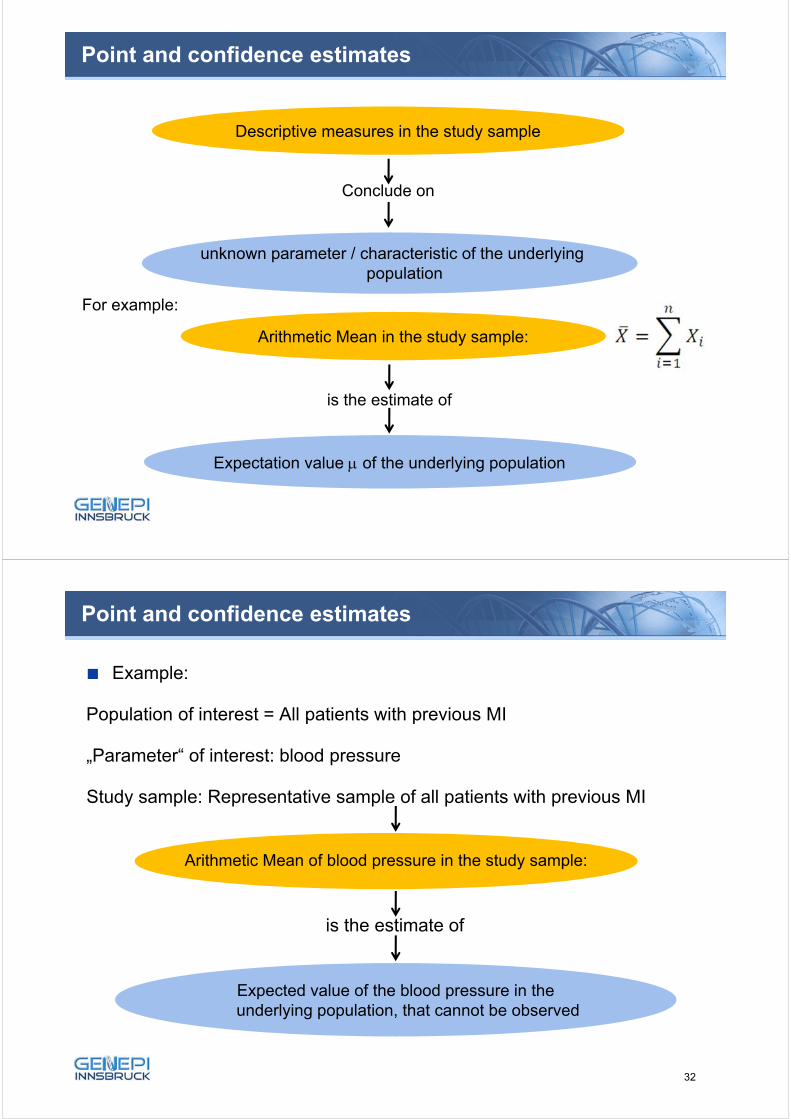
Arithmetic Mean in the study sample:
Descriptive measures in the study sample
Conclude on
unknown parameter / characteristic of the underlying population
For example:
is the estimate of
Expectation value of the underlying population
Point and confidence estimates
Example:
Population of interest = All patients with previous MI
„Parameter“ of interest: blood pressure
Study sample: Representative sample of all patients with previous MI
Expected value of the blood pressure in the underlying population, that cannot be observed
Arithmetic Mean of blood pressure in the study sample:
is the estimate of
32
Point and confidence estimates
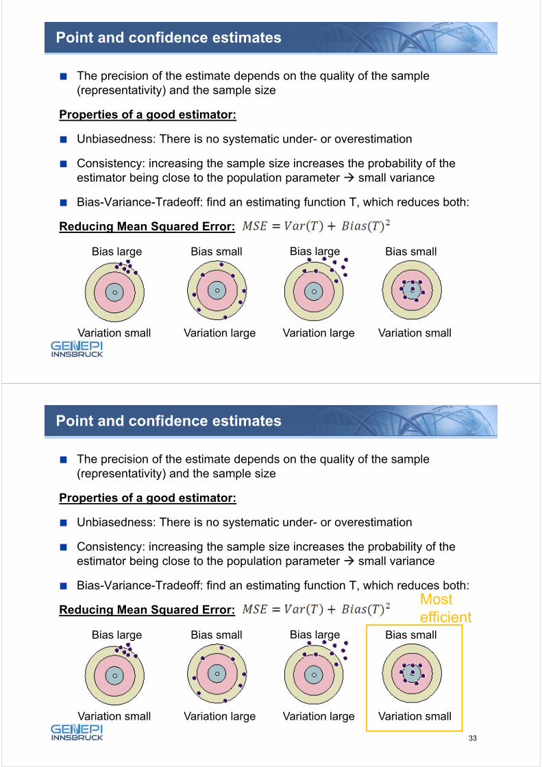
The precision of the estimate depends on the quality of the sample (representativity) and the sample size
Properties of a good estimator:
Unbiasedness: There is no systematic under- or overestimation
Consistency: increasing the sample size increases the probability of the estimator being close to the population parameter small variance
Bias-Variance-Tradeoff: find an estimating function T, which reduces both:
Reducing Mean Squared Error:
Bias large Bias large
Variation small
Bias small
Variation small Variation large Variation large
Bias small
Point and confidence estimates
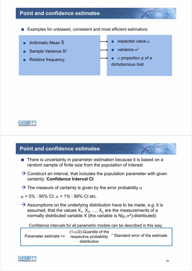
The precision of the estimate depends on the quality of the sample (representativity) and the sample size
Properties of a good estimator:
Unbiasedness: There is no systematic under- or overestimation
Consistency: increasing the sample size increases the probability of the estimator being close to the population parameter small variance
Bias-Variance-Tradeoff: find an estimating function T, which reduces both:
Reducing Mean Squared Error:
Bias large Bias large
Variation small
Bias small
Variation small Variation large Variation large
Bias small
Most efficient
33
Point and confidence estimates
Examples for unbiased, consistent and most efficient estimators:
Arithmetic Mean X
Sample Variance S2
Relative frequency
expected value
variance
proportion p of a
dichotomous trait
_
Point and confidence estimates
There is uncertainty in parameter estimation because it is based on a random sample of finite size from the population of interest
Construct an interval, that includes the population parameter with given certainty: Confidence Interval CI
The measure of certainty is given by the error probability
= 5% : 95% CI; = 1% : 99% CI etc.
Assumptions on the underlying distribution have to be made, e.g. it is assumed, that the values X1, X2, …, Xn are the measurements of a normally distributed variable X (the variable is N(,2)-distributed)
Confidence intervals for all parametric models can be described in this way:
Parameter estimate +/-(1-/2)-Quantile of the respective probability
distribution
* Standard error of the estimate
34
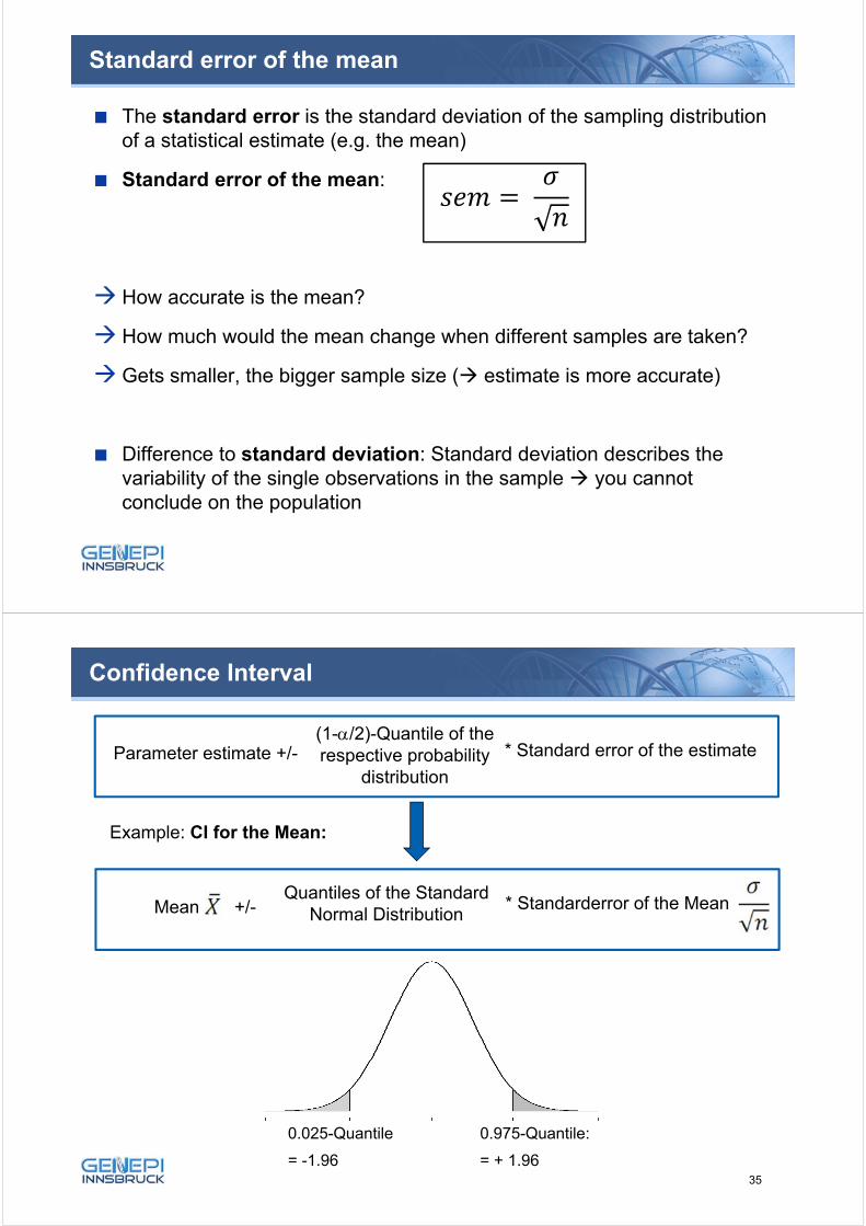
Standard error of the mean
The standard error is the standard deviation of the sampling distribution of a statistical estimate (e.g. the mean)
Standard error of the mean:
How accurate is the mean?
How much would the mean change when different samples are taken?
Gets smaller, the bigger sample size ( estimate is more accurate)
Difference to standard deviation: Standard deviation describes the variability of the single observations in the sample you cannot conclude on the population
Confidence Interval
0.025-Quantile
= -1.96
0.975-Quantile:
= + 1.96
Parameter estimate +/-(1-/2)-Quantile of the respective probability
distribution
* Standard error of the estimate
Mean +/-Quantiles of the Standard
Normal Distribution* Standarderror of the Mean
Example: CI for the Mean:
35
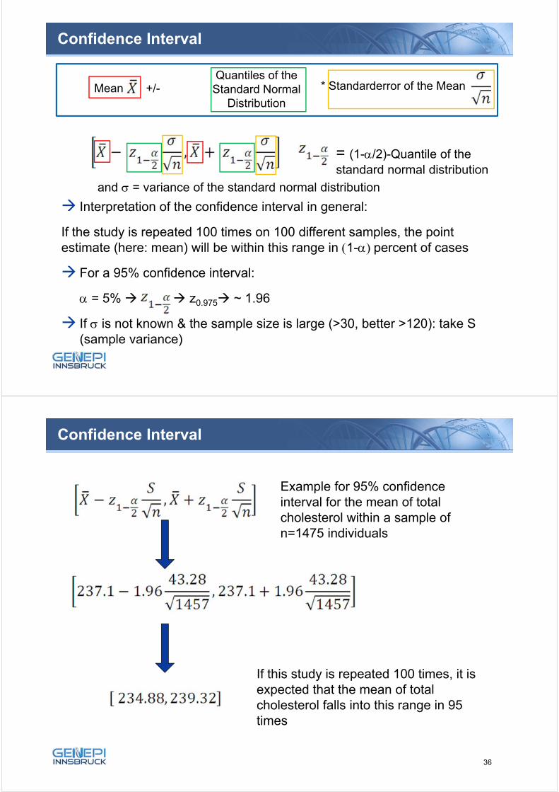
Confidence Interval
and = variance of the standard normal distribution
= (1-/2)-Quantile of the standard normal distribution
Interpretation of the confidence interval in general:
If the study is repeated 100 times on 100 different samples, the point estimate (here: mean) will be within this range in 1-percent of cases
For a 95% confidence interval:
= 5% z0.975 ~ 1.96
If is not known & the sample size is large (>30, better >120): take S (sample variance)
Mean +/-Quantiles of the
Standard Normal Distribution
* Standarderror of the Mean
Example for 95% confidence interval for the mean of total cholesterol within a sample of n=1475 individuals
If this study is repeated 100 times, it is expected that the mean of total cholesterol falls into this range in 95 times
Confidence Interval
36

Confidence Interval
Simulation Example: 95% CI for mean of body height in mean born 1993
Assumption: We know the „truth“: mean = 182 cm; σ = 7
A different sample is drawn 100 times (either with n=100 or n=20)
in 5 out of 100 experiments, the true expected mean value is not included
If you only conduct an experiement once (as usual), you do not know, ifthe true value is included (green bars) or not (red bars)
n=100 n=20
p 0.95 0.975 0.995
zp 1.64 1.96 2.58
Determine the 95%-CI for the following parameters:
Mean = 100
S = 15
n=25
95 % CI =
If you repeat an experiment 100 times with the assumption, that these parameters are true, how many times can you expect to observe a mean that is lower or higher than these confidence limits?
Quantiles of the standard normal distribution:
Confidence Interval: Exercise
37
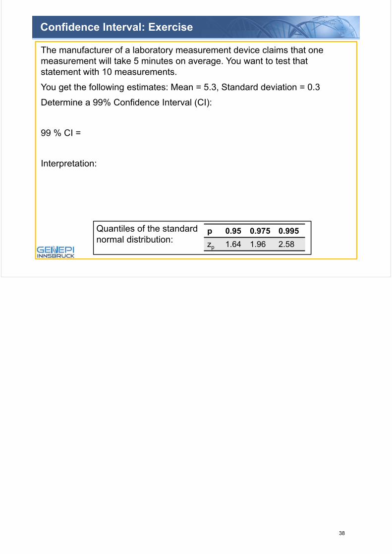
Confidence Interval: Exercise
p 0.95 0.975 0.995
zp 1.64 1.96 2.58
The manufacturer of a laboratory measurement device claims that one measurement will take 5 minutes on average. You want to test that statement with 10 measurements.
You get the following estimates: Mean = 5.3, Standard deviation = 0.3
Determine a 99% Confidence Interval (CI):
99 % CI =
Interpretation:
Quantiles of the standard normal distribution:
38