Embed Size (px)
Citation preview
S L I D E 0
Statistics in medicine
Lecture 3: Bivariate association : continuous variables
Fatma Shebl, MD, MS, MPH, PhD Assistant Professor Chronic Disease Epidemiology Department Yale School of Public Health [email protected]
S L I D E 1
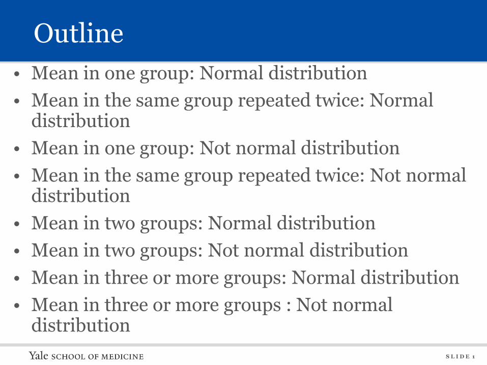
Outline • Mean in one group: Normal distribution • Mean in the same group repeated twice: Normal
distribution • Mean in one group: Not normal distribution • Mean in the same group repeated twice: Not normal
distribution • Mean in two groups: Normal distribution • Mean in two groups: Not normal distribution • Mean in three or more groups: Normal distribution • Mean in three or more groups : Not normal
distribution
S L I D E 2
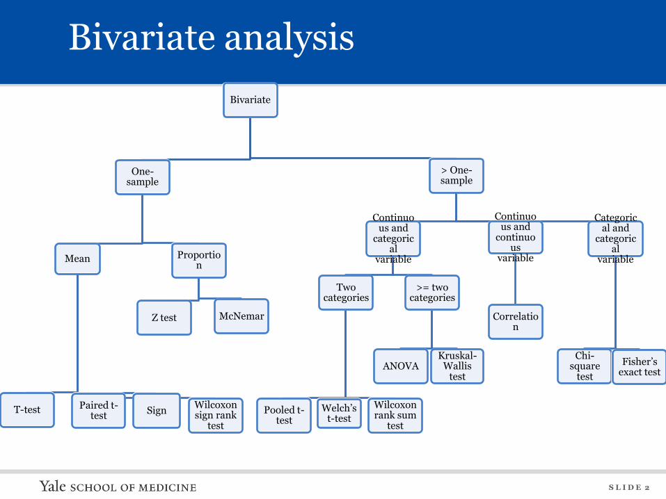
Bivariate analysis Bivariate
One-sample
Mean
T-test Paired t-test Sign Wilcoxon
sign rank test
Proportion
Z test McNemar
> One-sample
Continuous and
categorical
variable
Two categories
Pooled t-test
Welch’s t-test
Wilcoxon rank sum
test
>= two categories
ANOVA Kruskal-
Wallis test
Continuous and
continuous
variable
Correlation
Categorical and
categorical
variable
Chi-square
test Fisher’s
exact test
S L I D E 3
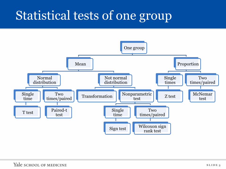
Statistical tests of one group
One group
Mean
Normal distribution
Single time
T test
Two times/paired
Paired-t test
Not normal distribution
Transformation Nonparametric test
Single time
Sign test
Two times/paired
Wilcoxon sign rank test
Proportion
Single times
Z test
Two times/paired
McNemar test
S L I D E 4
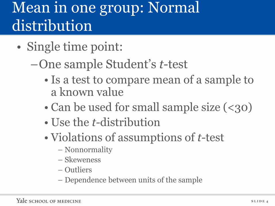
Mean in one group: Normal distribution • Single time point:
–One sample Student’s t-test • Is a test to compare mean of a sample to
a known value • Can be used for small sample size (<30) • Use the t-distribution • Violations of assumptions of t-test
– Nonnormality – Skeweness – Outliers – Dependence between units of the sample
S L I D E 5
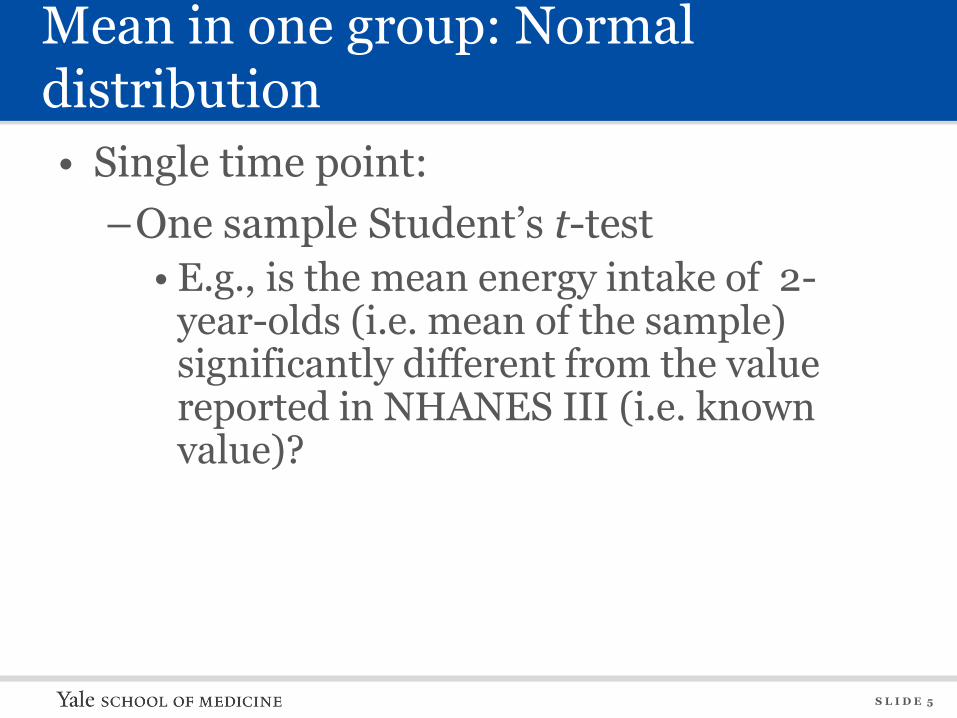
Mean in one group: Normal distribution • Single time point:
–One sample Student’s t-test • E.g., is the mean energy intake of 2-
year-olds (i.e. mean of the sample) significantly different from the value reported in NHANES III (i.e. known value)?
S L I D E 6
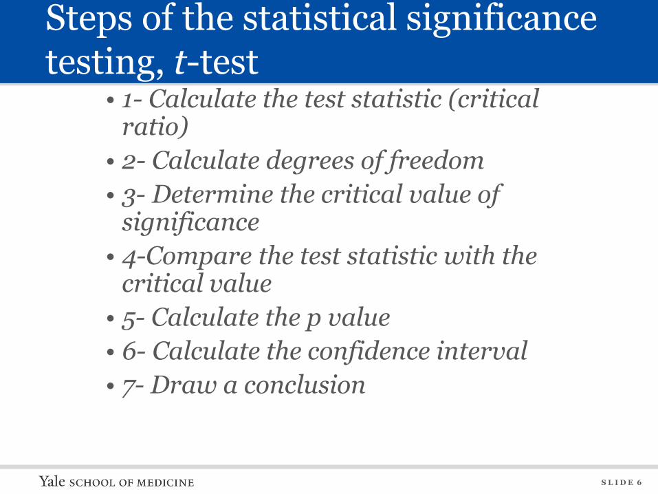
Steps of the statistical significance testing, t-test
• 1- Calculate the test statistic (critical ratio)
• 2- Calculate degrees of freedom • 3- Determine the critical value of
significance • 4-Compare the test statistic with the
critical value • 5- Calculate the p value • 6- Calculate the confidence interval • 7- Draw a conclusion
S L I D E 7
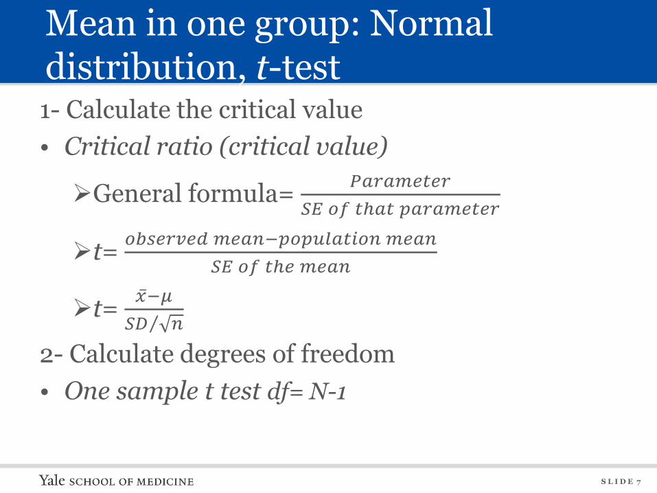
Mean in one group: Normal distribution, t-test 1- Calculate the critical value • Critical ratio (critical value)
¾General formula= 𝑃𝑎𝑟𝑎𝑚𝑒𝑡𝑒𝑟𝑆𝐸 𝑜𝑓 𝑡ℎ𝑎𝑡 𝑝𝑎𝑟𝑎𝑚𝑒𝑡𝑒𝑟
¾t= 𝑜𝑏𝑠𝑒𝑟𝑣𝑒𝑑 𝑚𝑒𝑎𝑛−𝑝𝑜𝑝𝑢𝑙𝑎𝑡𝑖𝑜𝑛 𝑚𝑒𝑎𝑛𝑆𝐸 𝑜𝑓 𝑡ℎ𝑒 𝑚𝑒𝑎𝑛
¾t= 𝑥 −𝜇𝑆𝐷 𝑛
2- Calculate degrees of freedom • One sample t test df= N-1
S L I D E 8
Mean in one group: Normal distribution
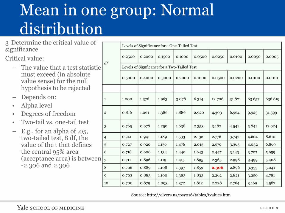
3-Determine the critical value of significance Critical value:
– The value that a test statistic must exceed (in absolute value sense) for the null hypothesis to be rejected
– Depends on: • Alpha level • Degrees of freedom • Two-tail vs. one-tail test – E.g., for an alpha of .05,
two-tailed test, 8 df, the value of the t that defines the central 95% area (acceptance area) is between -2.306 and 2.306
Source: http://elvers.us/psy216/tables/tvalues.htm
df
Levels of Significance for a One-Tailed Test
0.2500 0.2000 0.1500 0.1000 0.0500 0.0250 0.0100 0.0050 0.0005
Levels of Signficance for a Two-Tailed Test
0.5000 0.4000 0.3000 0.2000 0.1000 0.0500 0.0200 0.0100 0.0010
1 1.000 1.376 1.963 3.078 6.314 12.706 31.821 63.657 636.619
2 0.816 1.061 1.386 1.886 2.920 4.303 6.964 9.925 31.599
3 0.765 0.978 1.250 1.638 2.353 3.182 4.541 5.841 12.924
4 0.741 0.941 1.189 1.533 2.132 2.776 3.747 4.604 8.610
5 0.727 0.920 1.156 1.476 2.015 2.570 3.365 4.032 6.869
6 0.718 0.906 1.134 1.440 1.943 2.447 3.143 3.707 5.959
7 0.711 0.896 1.119 1.415 1.895 2.365 2.998 3.499 5.408
8 0.706 0.889 1.108 1.397 1.859 2.306 2.896 3.355 5.041
9 0.703 0.883 1.100 1.383 1.833 2.262 2.821 3.250 4.781
10 0.700 0.879 1.093 1.372 1.812 2.228 2.764 3.169 4.587
S L I D E 9
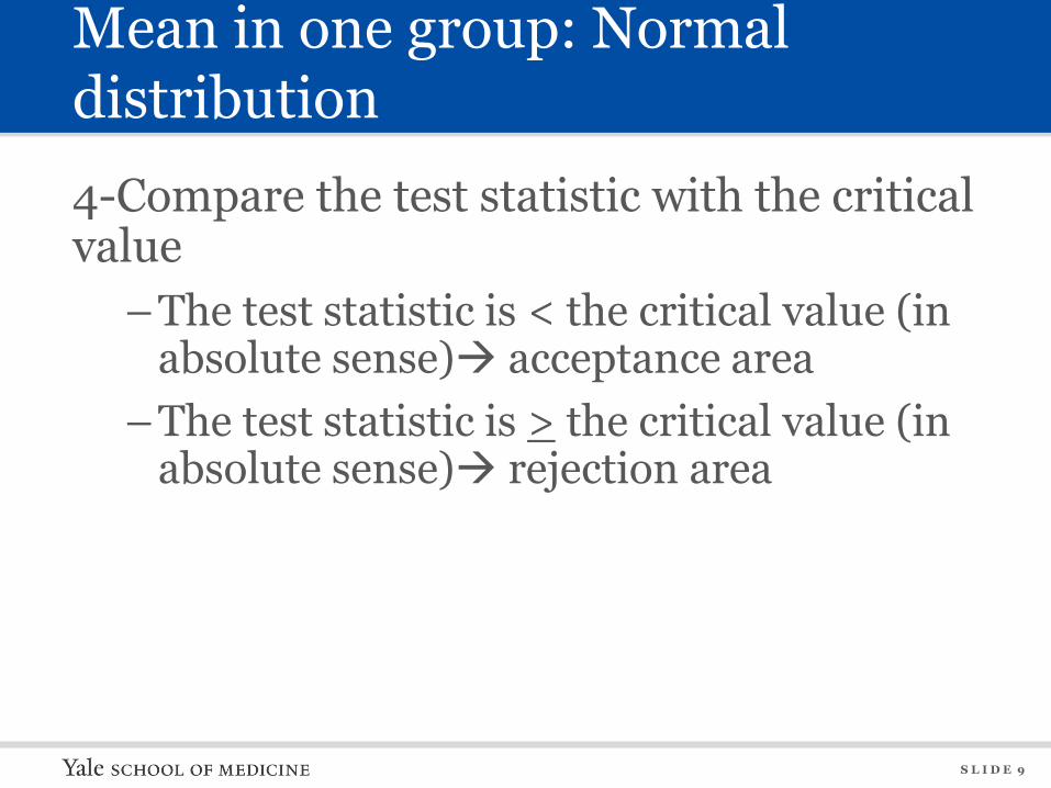
Mean in one group: Normal distribution 4-Compare the test statistic with the critical value
–The test statistic is < the critical value (in absolute sense)Æ acceptance area
–The test statistic is > the critical value (in absolute sense)Æ rejection area
S L I D E 10
Mean in one group: Normal distribution
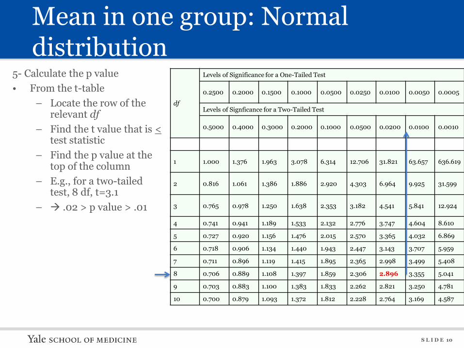
5- Calculate the p value • From the t-table
– Locate the row of the relevant df
– Find the t value that is < test statistic
– Find the p value at the top of the column
– E.g., for a two-tailed test, 8 df, t=3.1
– Æ .02 > p value > .01
df
Levels of Significance for a One-Tailed Test
0.2500 0.2000 0.1500 0.1000 0.0500 0.0250 0.0100 0.0050 0.0005
Levels of Signficance for a Two-Tailed Test
0.5000 0.4000 0.3000 0.2000 0.1000 0.0500 0.0200 0.0100 0.0010
1 1.000 1.376 1.963 3.078 6.314 12.706 31.821 63.657 636.619
2 0.816 1.061 1.386 1.886 2.920 4.303 6.964 9.925 31.599
3 0.765 0.978 1.250 1.638 2.353 3.182 4.541 5.841 12.924
4 0.741 0.941 1.189 1.533 2.132 2.776 3.747 4.604 8.610
5 0.727 0.920 1.156 1.476 2.015 2.570 3.365 4.032 6.869
6 0.718 0.906 1.134 1.440 1.943 2.447 3.143 3.707 5.959
7 0.711 0.896 1.119 1.415 1.895 2.365 2.998 3.499 5.408
8 0.706 0.889 1.108 1.397 1.859 2.306 2.896 3.355 5.041
9 0.703 0.883 1.100 1.383 1.833 2.262 2.821 3.250 4.781
10 0.700 0.879 1.093 1.372 1.812 2.228 2.764 3.169 4.587
S L I D E 11
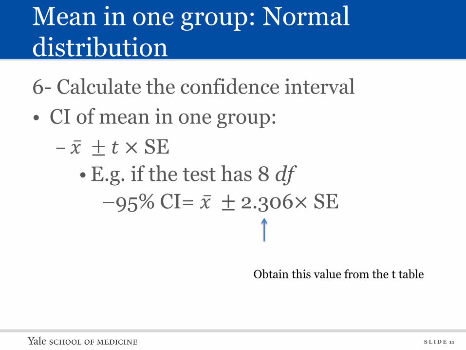
Mean in one group: Normal distribution 6- Calculate the confidence interval • CI of mean in one group:
– 𝑥 ± 𝑡 × SE • E.g. if the test has 8 df
–95% CI= 𝑥 ± 2.306× SE
Obtain this value from the t table
S L I D E 12
Mean in one group: Normal distribution 7- Draw a conclusion • Reject or fail to reject the null hypothesis
– Fail to reject the null • If the p value > alpha level • If the confidence interval crosses the 0
– Reject the null • If the p value < alpha level • If the confidence interval does not include
0
S L I D E 13
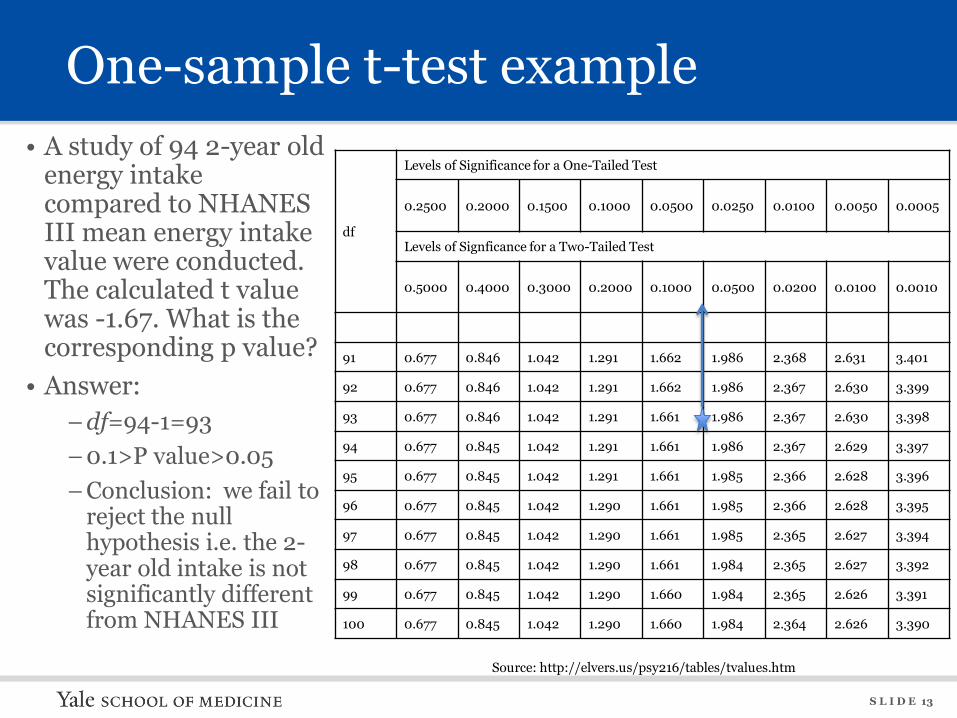
One-sample t-test example • A study of 94 2-year old
energy intake compared to NHANES III mean energy intake value were conducted. The calculated t value was -1.67. What is the corresponding p value?
• Answer: – df=94-1=93 – 0.1>P value>0.05 – Conclusion: we fail to
reject the null hypothesis i.e. the 2-year old intake is not significantly different from NHANES III
Source: http://elvers.us/psy216/tables/tvalues.htm
df
Levels of Significance for a One-Tailed Test
0.2500 0.2000 0.1500 0.1000 0.0500 0.0250 0.0100 0.0050 0.0005
Levels of Signficance for a Two-Tailed Test
0.5000 0.4000 0.3000 0.2000 0.1000 0.0500 0.0200 0.0100 0.0010
91 0.677 0.846 1.042 1.291 1.662 1.986 2.368 2.631 3.401
92 0.677 0.846 1.042 1.291 1.662 1.986 2.367 2.630 3.399
93 0.677 0.846 1.042 1.291 1.661 1.986 2.367 2.630 3.398
94 0.677 0.845 1.042 1.291 1.661 1.986 2.367 2.629 3.397
95 0.677 0.845 1.042 1.291 1.661 1.985 2.366 2.628 3.396
96 0.677 0.845 1.042 1.290 1.661 1.985 2.366 2.628 3.395
97 0.677 0.845 1.042 1.290 1.661 1.985 2.365 2.627 3.394
98 0.677 0.845 1.042 1.290 1.661 1.984 2.365 2.627 3.392
99 0.677 0.845 1.042 1.290 1.660 1.984 2.365 2.626 3.391
100 0.677 0.845 1.042 1.290 1.660 1.984 2.364 2.626 3.390
S L I D E 14
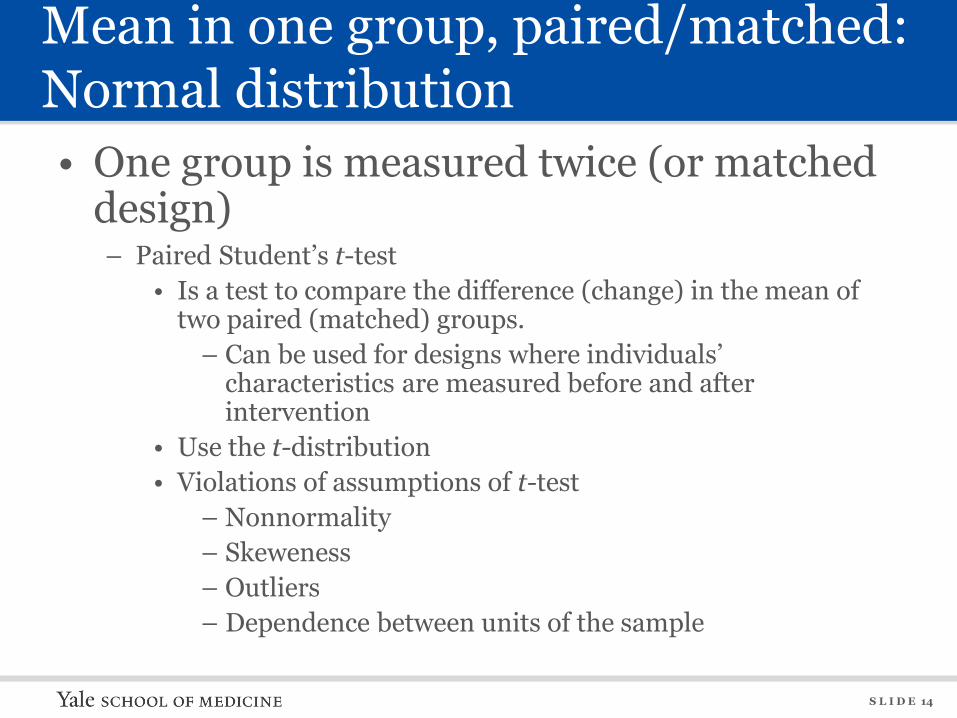
Mean in one group, paired/matched: Normal distribution • One group is measured twice (or matched
design) – Paired Student’s t-test
• Is a test to compare the difference (change) in the mean of two paired (matched) groups.
– Can be used for designs where individuals’ characteristics are measured before and after intervention
• Use the t-distribution • Violations of assumptions of t-test
– Nonnormality – Skeweness – Outliers – Dependence between units of the sample
S L I D E 15
Mean in one group, paired/matched: Normal distribution, paired t-test
• One group is measured twice (or matched design): –Paired Student’s t-test
• E.g., Is there a change in serum LDL levels after cholecystectomy?
S L I D E 16
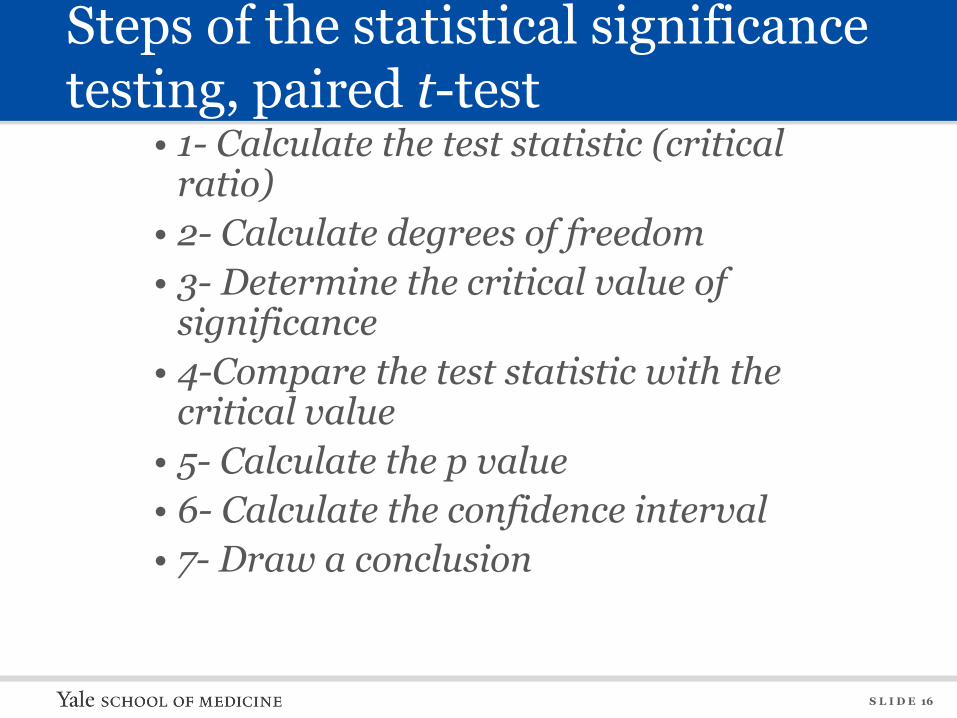
Steps of the statistical significance testing, paired t-test
• 1- Calculate the test statistic (critical ratio)
• 2- Calculate degrees of freedom • 3- Determine the critical value of
significance • 4-Compare the test statistic with the
critical value • 5- Calculate the p value • 6- Calculate the confidence interval • 7- Draw a conclusion
S L I D E 17
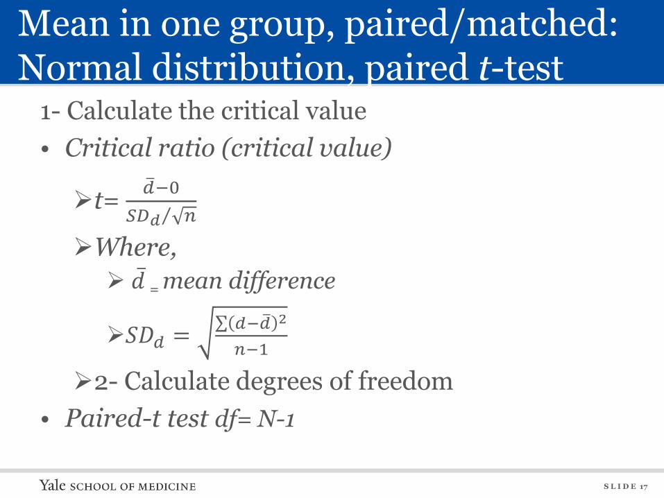
Mean in one group, paired/matched: Normal distribution, paired t-test
1- Calculate the critical value • Critical ratio (critical value)
¾t= 𝑑 −0𝑆𝐷𝑑 𝑛
¾Where, ¾ 𝑑 = mean difference
¾𝑆𝐷𝑑 = 𝑑−𝑑 2
𝑛−1
¾2- Calculate degrees of freedom • Paired-t test df= N-1
S L I D E 18
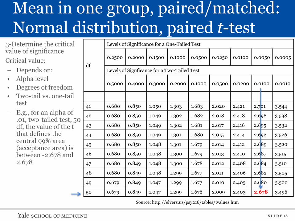
Mean in one group, paired/matched: Normal distribution, paired t-test
3-Determine the critical value of significance Critical value: – Depends on: • Alpha level • Degrees of freedom • Two-tail vs. one-tail
test – E.g., for an alpha of
.01, two-tailed test, 50 df, the value of the t that defines the central 99% area (acceptance area) is between -2.678 and 2.678
Source: http://elvers.us/psy216/tables/tvalues.htm
df
Levels of Significance for a One-Tailed Test
0.2500 0.2000 0.1500 0.1000 0.0500 0.0250 0.0100 0.0050 0.0005
Levels of Signficance for a Two-Tailed Test
0.5000 0.4000 0.3000 0.2000 0.1000 0.0500 0.0200 0.0100 0.0010
41 0.680 0.850 1.050 1.303 1.683 2.020 2.421 2.701 3.544
42 0.680 0.850 1.049 1.302 1.682 2.018 2.418 2.698 3.538
43 0.680 0.850 1.049 1.302 1.681 2.017 2.416 2.695 3.532
44 0.680 0.850 1.049 1.301 1.680 2.015 2.414 2.692 3.526
45 0.680 0.850 1.048 1.301 1.679 2.014 2.412 2.689 3.520
46 0.680 0.850 1.048 1.300 1.679 2.013 2.410 2.687 3.515
47 0.680 0.849 1.048 1.300 1.678 2.012 2.408 2.684 3.510
48 0.680 0.849 1.048 1.299 1.677 2.011 2.406 2.682 3.505
49 0.679 0.849 1.047 1.299 1.677 2.010 2.405 2.680 3.500
50 0.679 0.849 1.047 1.299 1.676 2.009 2.403 2.678 3.496
S L I D E 19
Mean in one group, paired/matched: Normal distribution, paired t-test
4-Compare the test statistic with the critical value
–The test statistic is < the critical value (in absolute sense)Æ acceptance area
–The test statistic is > the critical value (in absolute sense)Æ rejection area
S L I D E 20
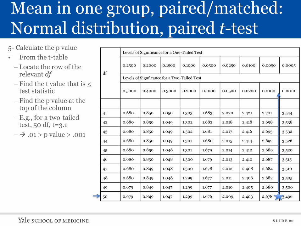
Mean in one group, paired/matched: Normal distribution, paired t-test
5- Calculate the p value • From the t-table
– Locate the row of the relevant df
– Find the t value that is < test statistic
– Find the p value at the top of the column
– E.g., for a two-tailed test, 50 df, t=3.1
–Æ .01 > p value > .001
df
Levels of Significance for a One-Tailed Test
0.2500 0.2000 0.1500 0.1000 0.0500 0.0250 0.0100 0.0050 0.0005
Levels of Signficance for a Two-Tailed Test
0.5000 0.4000 0.3000 0.2000 0.1000 0.0500 0.0200 0.0100 0.0010
41 0.680 0.850 1.050 1.303 1.683 2.020 2.421 2.701 3.544
42 0.680 0.850 1.049 1.302 1.682 2.018 2.418 2.698 3.538
43 0.680 0.850 1.049 1.302 1.681 2.017 2.416 2.695 3.532
44 0.680 0.850 1.049 1.301 1.680 2.015 2.414 2.692 3.526
45 0.680 0.850 1.048 1.301 1.679 2.014 2.412 2.689 3.520
46 0.680 0.850 1.048 1.300 1.679 2.013 2.410 2.687 3.515
47 0.680 0.849 1.048 1.300 1.678 2.012 2.408 2.684 3.510
48 0.680 0.849 1.048 1.299 1.677 2.011 2.406 2.682 3.505
49 0.679 0.849 1.047 1.299 1.677 2.010 2.405 2.680 3.500
50 0.679 0.849 1.047 1.299 1.676 2.009 2.403 2.678 3.496
S L I D E 21
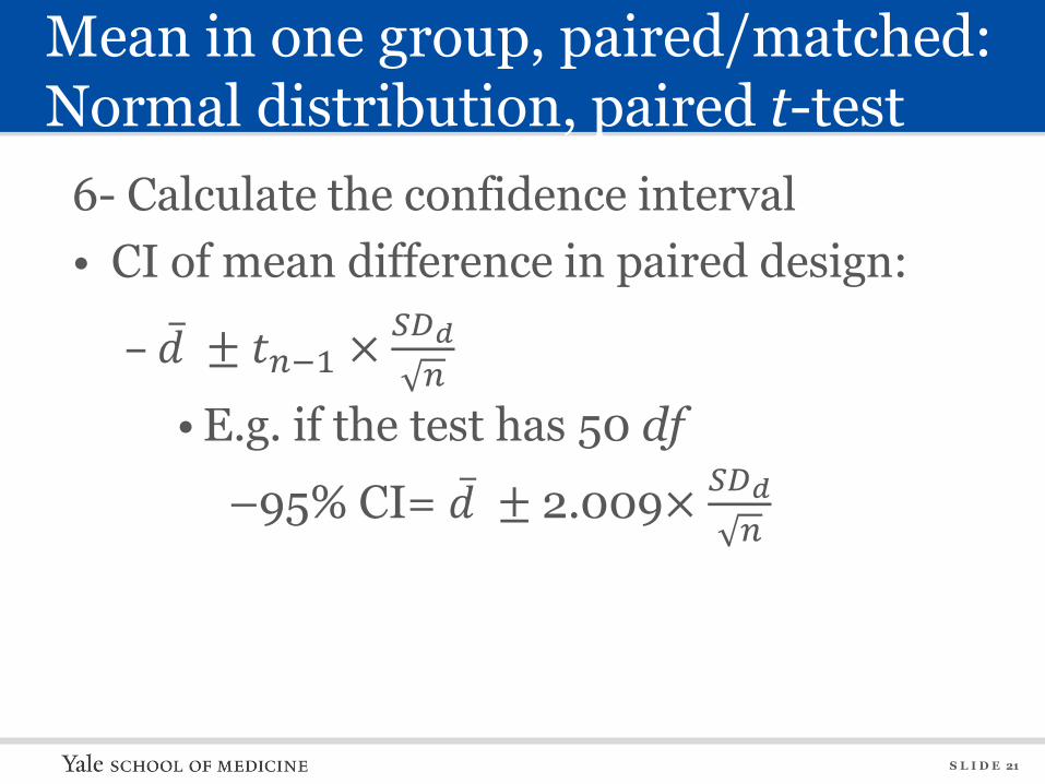
Mean in one group, paired/matched: Normal distribution, paired t-test
6- Calculate the confidence interval • CI of mean difference in paired design:
– 𝑑 ± 𝑡𝑛−1 × 𝑆𝐷𝑑𝑛
• E.g. if the test has 50 df
–95% CI= 𝑑 ± 2.009× 𝑆𝐷𝑑𝑛
S L I D E 22
Mean in one group, paired/matched: Normal distribution, paired t-test
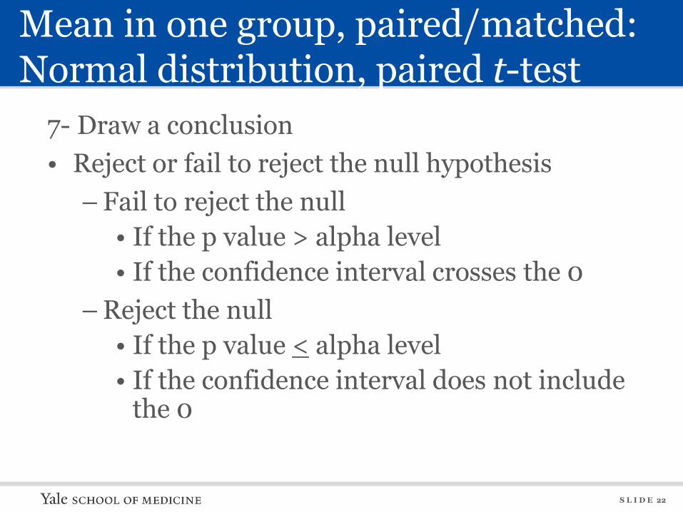
7- Draw a conclusion • Reject or fail to reject the null hypothesis
– Fail to reject the null • If the p value > alpha level • If the confidence interval crosses the 0
– Reject the null • If the p value < alpha level • If the confidence interval does not include
the 0
S L I D E 23
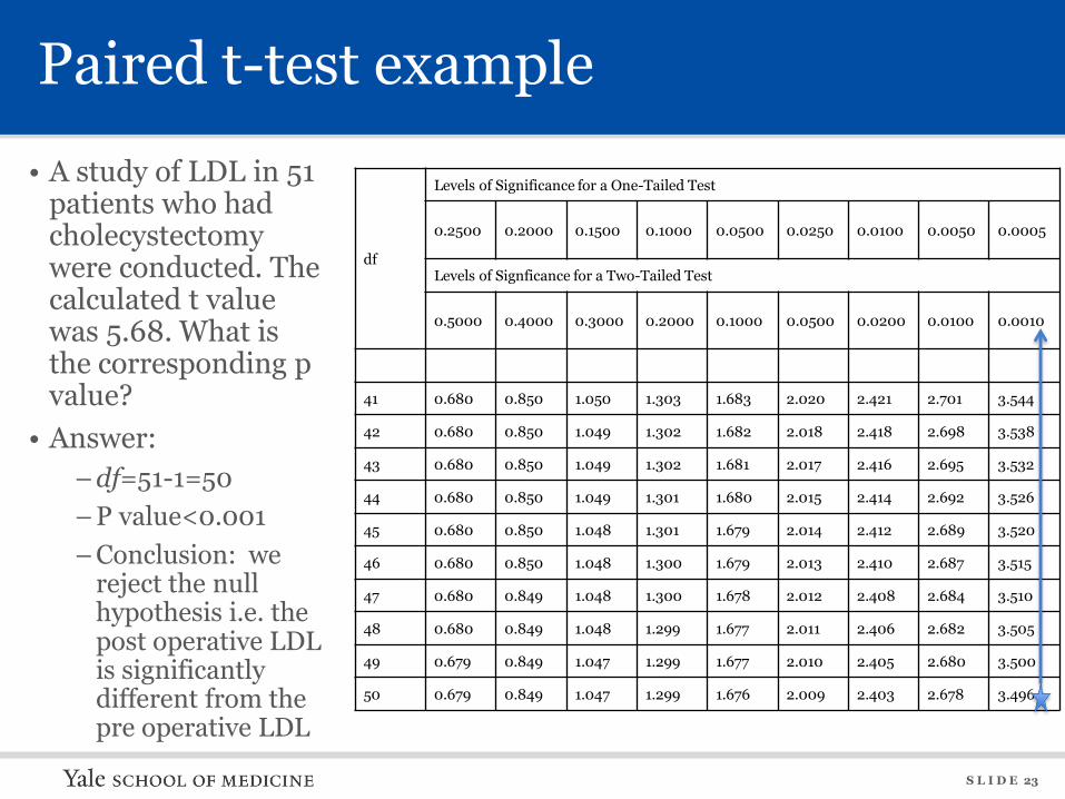
Paired t-test example
• A study of LDL in 51 patients who had cholecystectomy were conducted. The calculated t value was 5.68. What is the corresponding p value?
• Answer: – df=51-1=50 – P value<0.001 – Conclusion: we
reject the null hypothesis i.e. the post operative LDL is significantly different from the pre operative LDL
df
Levels of Significance for a One-Tailed Test
0.2500 0.2000 0.1500 0.1000 0.0500 0.0250 0.0100 0.0050 0.0005
Levels of Signficance for a Two-Tailed Test
0.5000 0.4000 0.3000 0.2000 0.1000 0.0500 0.0200 0.0100 0.0010
41 0.680 0.850 1.050 1.303 1.683 2.020 2.421 2.701 3.544
42 0.680 0.850 1.049 1.302 1.682 2.018 2.418 2.698 3.538
43 0.680 0.850 1.049 1.302 1.681 2.017 2.416 2.695 3.532
44 0.680 0.850 1.049 1.301 1.680 2.015 2.414 2.692 3.526
45 0.680 0.850 1.048 1.301 1.679 2.014 2.412 2.689 3.520
46 0.680 0.850 1.048 1.300 1.679 2.013 2.410 2.687 3.515
47 0.680 0.849 1.048 1.300 1.678 2.012 2.408 2.684 3.510
48 0.680 0.849 1.048 1.299 1.677 2.011 2.406 2.682 3.505
49 0.679 0.849 1.047 1.299 1.677 2.010 2.405 2.680 3.500
50 0.679 0.849 1.047 1.299 1.676 2.009 2.403 2.678 3.496
S L I D E 24
Median in one group: Not normal distribution • Single time point:
–Sign test • Is a nonparametric (distribution free)
test to compare median of a sample to a known value
• Indications: single sample with –Abnormal distribution –Skewed data –Outliers
S L I D E 25
Median in one group: Not normal distribution • Single time point:
–Sign test • Because the median is used, binomial
distribution with π=.5 could be used • If sample size is large, z distribution
could be used • E.g., is the median energy intake of 2-
year-olds significantly different from the value reported in NHANES III?
S L I D E 26
Steps of the statistical significance testing, sign test
• 1- Calculate the test statistic • 2- Determine the critical value of
significance • 3-Compare the test statistic with the
critical value • 4- Calculate the p value • 5- Draw a conclusion
S L I D E 27
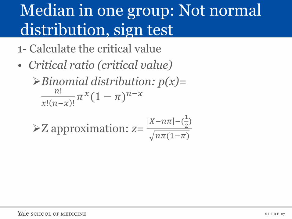
Median in one group: Not normal distribution, sign test 1- Calculate the critical value • Critical ratio (critical value) ¾Binomial distribution: p(x)=
𝑛!𝑥! 𝑛−𝑥 ! 𝜋
𝑥(1 − 𝜋)𝑛−𝑥
¾Z approximation: z= 𝑋−𝑛𝜋 −(12)
𝑛𝜋(1−𝜋)
S L I D E 28
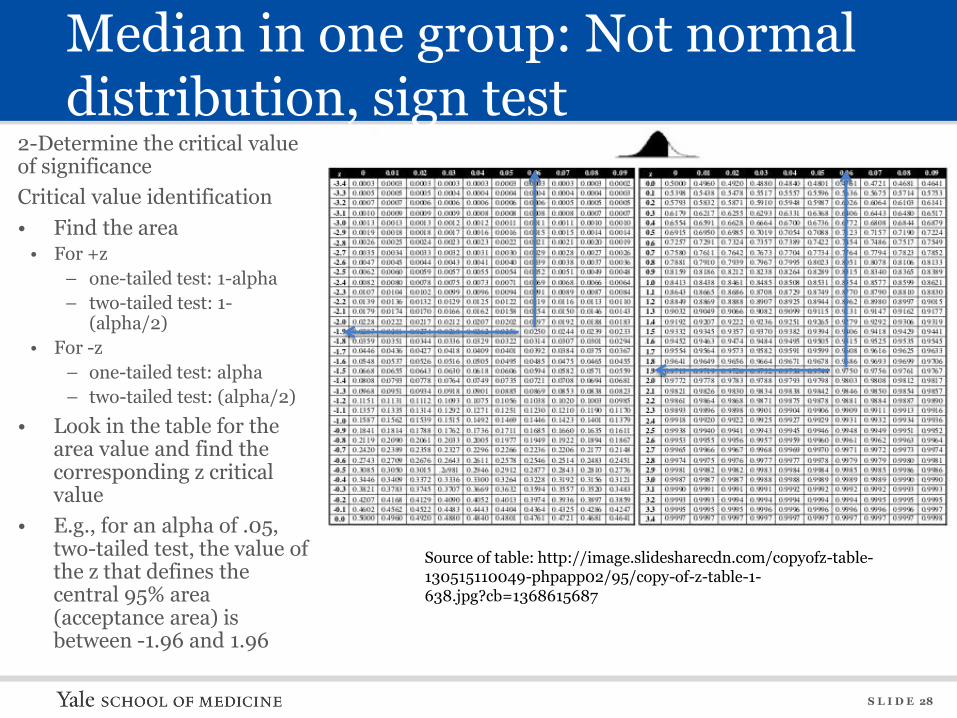
Median in one group: Not normal distribution, sign test
2-Determine the critical value of significance Critical value identification • Find the area
• For +z – one-tailed test: 1-alpha – two-tailed test: 1-
(alpha/2) • For -z
– one-tailed test: alpha – two-tailed test: (alpha/2)
• Look in the table for the area value and find the corresponding z critical value
• E.g., for an alpha of .05, two-tailed test, the value of the z that defines the central 95% area (acceptance area) is between -1.96 and 1.96
Source of table: http://image.slidesharecdn.com/copyofz-table-130515110049-phpapp02/95/copy-of-z-table-1-638.jpg?cb=1368615687
S L I D E 29
Median in one group: Not normal distribution, sign test 3-Compare the test statistic with the critical value
–The test statistic is < the critical value (in absolute sense)Æ acceptance area
–The test statistic is > the critical value (in absolute sense)Æ rejection area
S L I D E 30
Median in one group: Not normal distribution, sign test
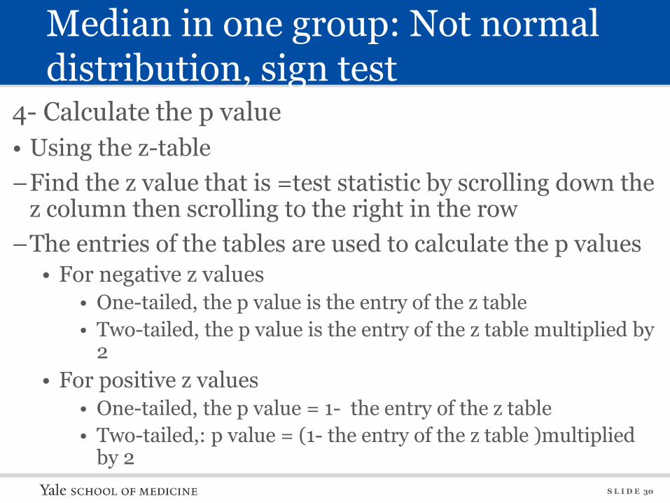
4- Calculate the p value • Using the z-table –Find the z value that is =test statistic by scrolling down the
z column then scrolling to the right in the row –The entries of the tables are used to calculate the p values
• For negative z values • One-tailed, the p value is the entry of the z table • Two-tailed, the p value is the entry of the z table multiplied by
2 • For positive z values
• One-tailed, the p value = 1- the entry of the z table • Two-tailed,: p value = (1- the entry of the z table )multiplied
by 2
S L I D E 31
Median in one group: Not normal distribution, sign test
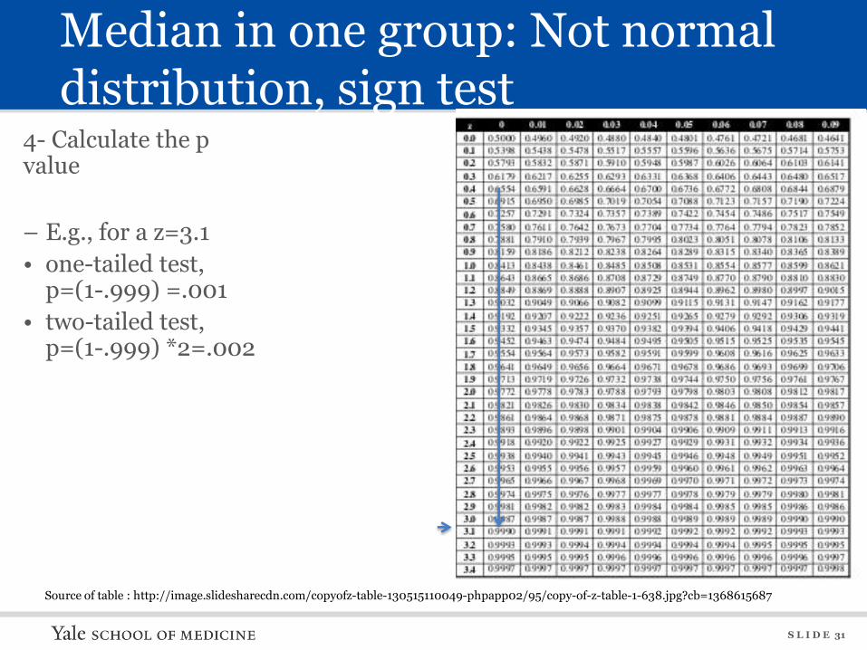
4- Calculate the p value
– E.g., for a z=3.1 • one-tailed test,
p=(1-.999) =.001 • two-tailed test,
p=(1-.999) *2=.002
Source of table : http://image.slidesharecdn.com/copyofz-table-130515110049-phpapp02/95/copy-of-z-table-1-638.jpg?cb=1368615687
S L I D E 32
Median in one group: N0t normal distribution, sign test 5- Draw a conclusion • Reject or fail to reject the null hypothesis
– Fail to reject the null • If the p value > alpha level
– Reject the null • If the p value < alpha level
S L I D E 33
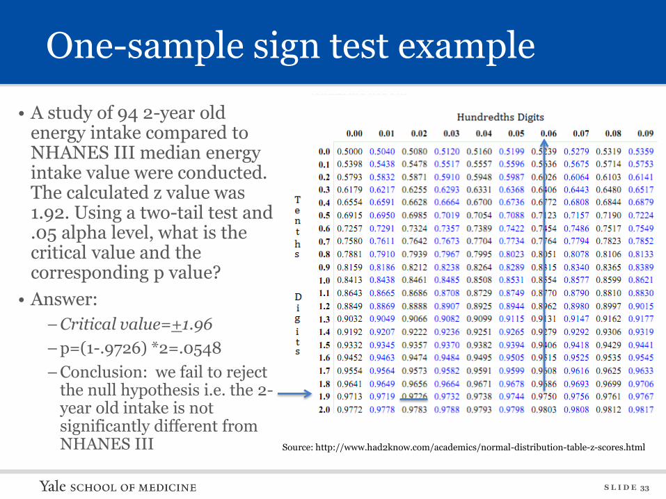
One-sample sign test example
• A study of 94 2-year old energy intake compared to NHANES III median energy intake value were conducted. The calculated z value was 1.92. Using a two-tail test and .05 alpha level, what is the critical value and the corresponding p value?
• Answer: – Critical value=+1.96 – p=(1-.9726) *2=.0548 – Conclusion: we fail to reject
the null hypothesis i.e. the 2-year old intake is not significantly different from NHANES III
Source: http://www.had2know.com/academics/normal-distribution-table-z-scores.html
S L I D E 34
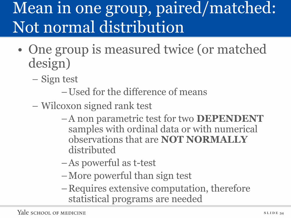
Mean in one group, paired/matched: Not normal distribution • One group is measured twice (or matched
design) – Sign test
–Used for the difference of means – Wilcoxon signed rank test
–A non parametric test for two DEPENDENT samples with ordinal data or with numerical observations that are NOT NORMALLY distributed
–As powerful as t-test –More powerful than sign test –Requires extensive computation, therefore
statistical programs are needed
S L I D E 35
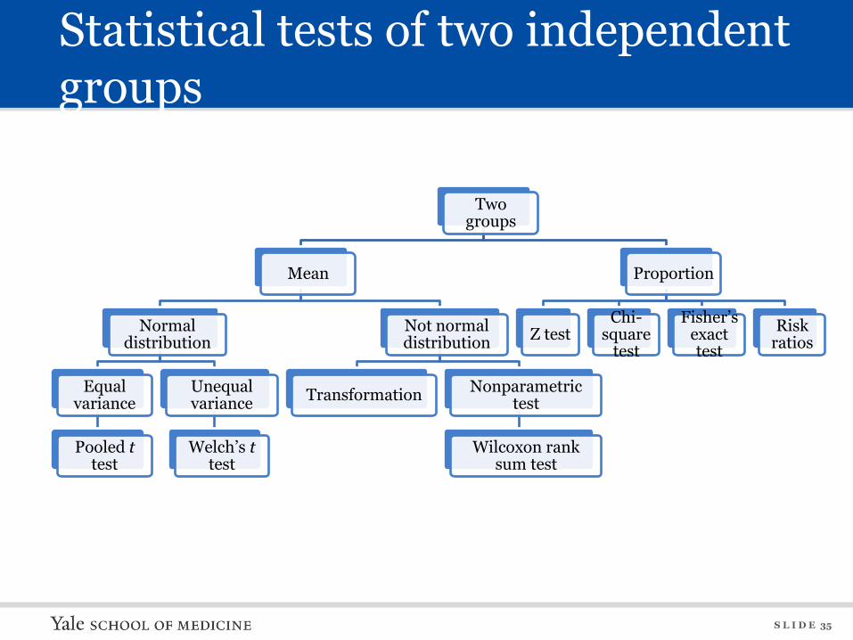
Statistical tests of two independent groups
Two groups
Mean
Normal distribution
Equal variance
Pooled t test
Unequal variance
Welch’s t test
Not normal distribution
Transformation Nonparametric test
Wilcoxon rank sum test
Proportion
Z test Chi-
square test
Fisher’s exact test
Risk ratios
S L I D E 36
Mean in two groups: Normal distribution
–Two-sample t-test • Is a test to compare means of two small
samples • Can be used for small sample size (<30) • Use the t-distribution • Violations of assumptions of t-test
– Nonnormality in either group: if sample size>30 it might be okay
– Equal variance in the two groups – Dependence between units of the sample
S L I D E 37
Mean in two groups: Normal distribution, t-test • Two-sample t-test:
• E.g., Did women who receive paracervical block prior to the cryosurgery have less severe total cramping than women who did not?
S L I D E 38
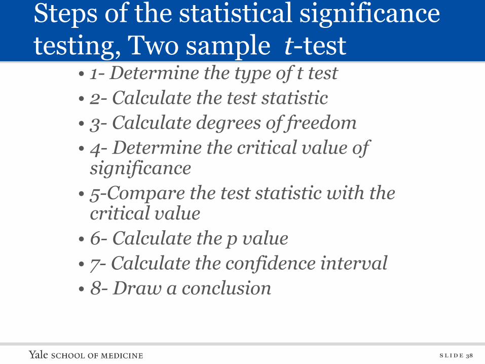
Steps of the statistical significance testing, Two sample t-test
• 1- Determine the type of t test • 2- Calculate the test statistic • 3- Calculate degrees of freedom • 4- Determine the critical value of
significance • 5-Compare the test statistic with the
critical value • 6- Calculate the p value • 7- Calculate the confidence interval • 8- Draw a conclusion
S L I D E 39
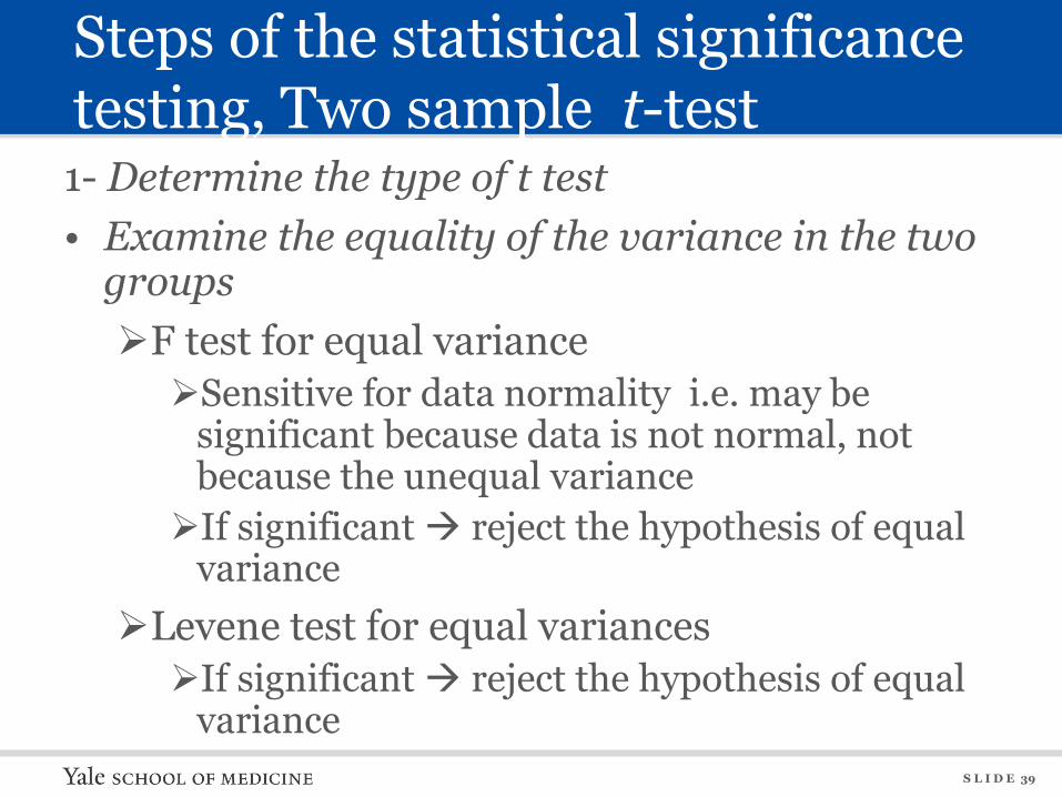
Steps of the statistical significance testing, Two sample t-test 1- Determine the type of t test • Examine the equality of the variance in the two
groups ¾F test for equal variance ¾Sensitive for data normality i.e. may be
significant because data is not normal, not because the unequal variance ¾If significant Æ reject the hypothesis of equal
variance ¾Levene test for equal variances ¾If significant Æ reject the hypothesis of equal
variance
S L I D E 40
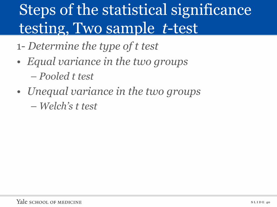
Steps of the statistical significance testing, Two sample t-test 1- Determine the type of t test • Equal variance in the two groups
– Pooled t test • Unequal variance in the two groups
– Welch’s t test
S L I D E 41
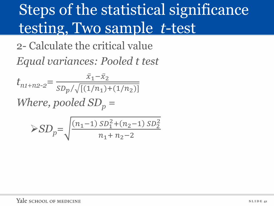
Steps of the statistical significance testing, Two sample t-test 2- Calculate the critical value Equal variances: Pooled t test
tn1+n2-2= 𝑥 1−𝑥 2𝑆𝐷𝑝 [(1/𝑛1)+(1/𝑛2)]
Where, pooled SDp =
¾SDp= 𝑛1−1 𝑆𝐷12+ 𝑛2−1 𝑆𝐷2
2
𝑛1+ 𝑛2−2
S L I D E 42
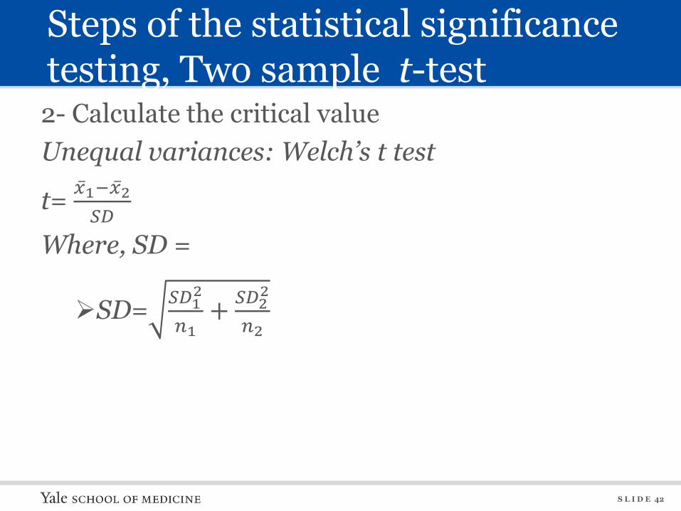
Steps of the statistical significance testing, Two sample t-test 2- Calculate the critical value Unequal variances: Welch’s t test
t= 𝑥 1−𝑥 2𝑆𝐷
Where, SD =
¾SD= 𝑆𝐷12
𝑛1+ 𝑆𝐷2
2
𝑛2
S L I D E 43
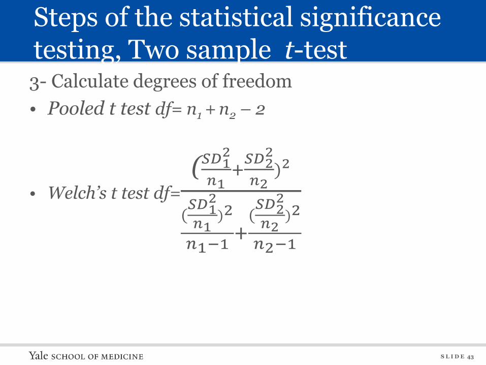
Steps of the statistical significance testing, Two sample t-test 3- Calculate degrees of freedom • Pooled t test df= n1 + n2 – 2
• Welch’s t test df=(𝑆𝐷1
2
𝑛1+𝑆𝐷2
2
𝑛2)2
(𝑆𝐷12
𝑛1)2
𝑛1−1 +(𝑆𝐷2
2
𝑛2)2
𝑛2−1
S L I D E 44
Steps of the statistical significance testing, Two sample t-test 4-Determine the critical value of significance, using t-distribution table based on
– Alpha level – df – Two-tail or one-tail
5-Compare the test statistic with the critical value – The test statistic is < the critical value (in
absolute sense)Æ acceptance area – The test statistic is > the critical value (in
absolute sense)Æ rejection area
S L I D E 45
Steps of the statistical significance testing, Two sample t-test
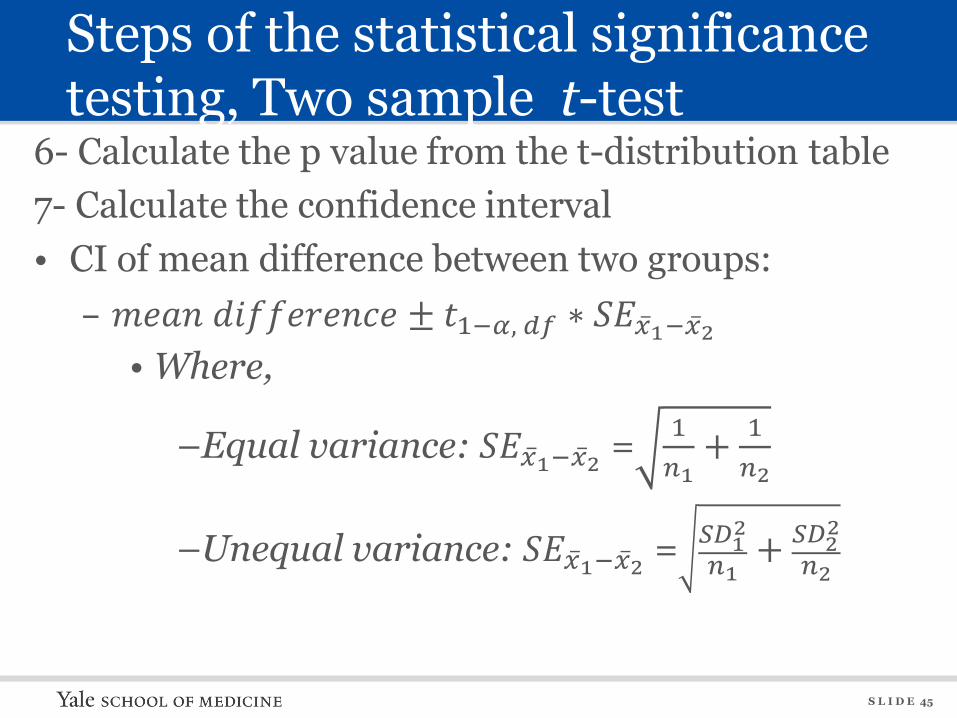
6- Calculate the p value from the t-distribution table 7- Calculate the confidence interval • CI of mean difference between two groups:
– 𝑚𝑒𝑎𝑛 𝑑𝑖𝑓𝑓𝑒𝑟𝑒𝑛𝑐𝑒 ± 𝑡1−𝛼, 𝑑𝑓 ∗ 𝑆𝐸𝑥 1−𝑥 2 • Where,
–Equal variance: 𝑆𝐸𝑥 1−𝑥 2 =1𝑛1
+ 1𝑛2
–Unequal variance: 𝑆𝐸𝑥 1−𝑥 2 =𝑆𝐷1
2
𝑛1+ 𝑆𝐷2
2
𝑛2
S L I D E 46
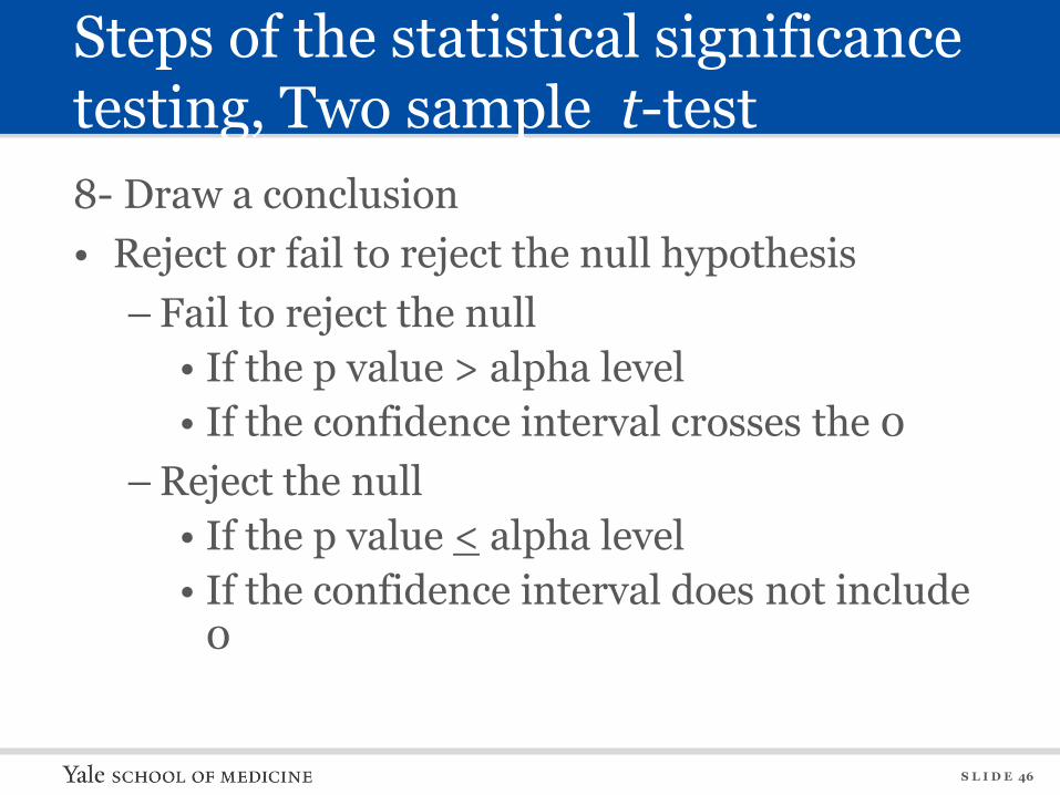
Steps of the statistical significance testing, Two sample t-test 8- Draw a conclusion • Reject or fail to reject the null hypothesis
– Fail to reject the null • If the p value > alpha level • If the confidence interval crosses the 0
– Reject the null • If the p value < alpha level • If the confidence interval does not include
0
S L I D E 47
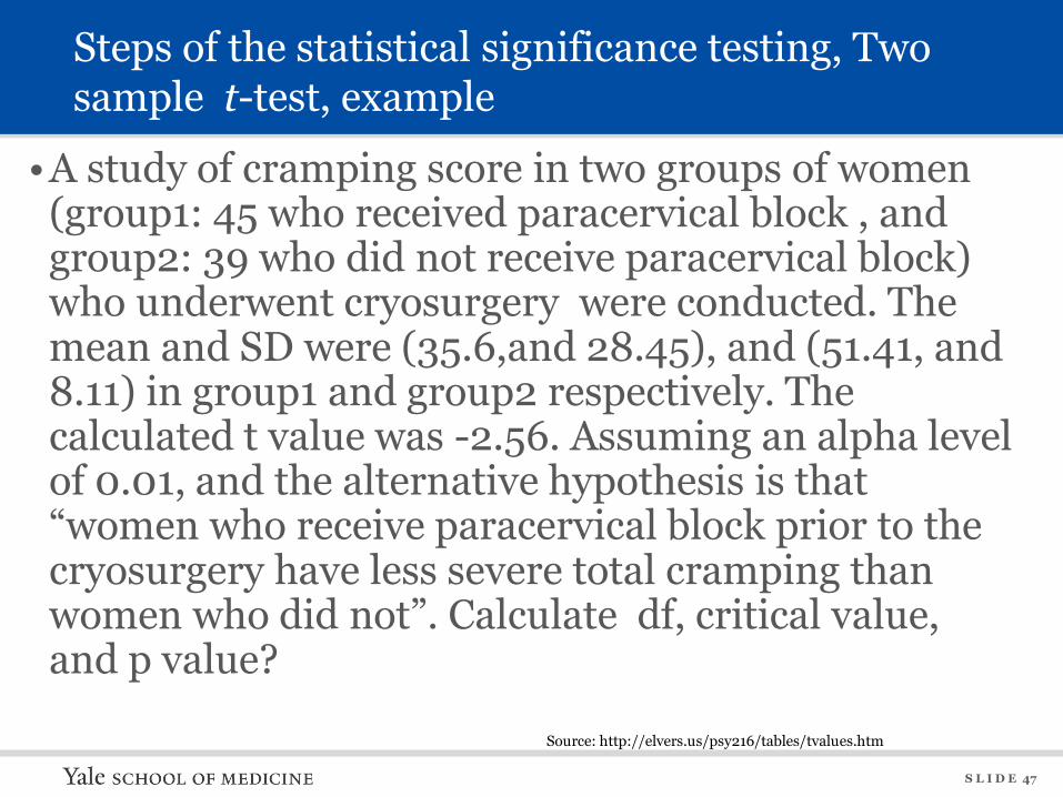
Steps of the statistical significance testing, Two sample t-test, example
•A study of cramping score in two groups of women (group1: 45 who received paracervical block , and group2: 39 who did not receive paracervical block) who underwent cryosurgery were conducted. The mean and SD were (35.6,and 28.45), and (51.41, and 8.11) in group1 and group2 respectively. The calculated t value was -2.56. Assuming an alpha level of 0.01, and the alternative hypothesis is that “women who receive paracervical block prior to the cryosurgery have less severe total cramping than women who did not”. Calculate df, critical value, and p value?
Source: http://elvers.us/psy216/tables/tvalues.htm
S L I D E 48
Steps of the statistical significance testing, Two sample t-test, example
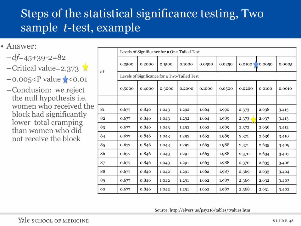
• Answer: –df=45+39-2=82 –Critical value=2.373 –0.005<P value <0.01 –Conclusion: we reject
the null hypothesis i.e. women who received the block had significantly lower total cramping than women who did not receive the block
Source: http://elvers.us/psy216/tables/tvalues.htm
df
Levels of Significance for a One-Tailed Test
0.2500 0.2000 0.1500 0.1000 0.0500 0.0250 0.0100 0.0050 0.0005
Levels of Signficance for a Two-Tailed Test
0.5000 0.4000 0.3000 0.2000 0.1000 0.0500 0.0200 0.0100 0.0010
81 0.677 0.846 1.043 1.292 1.664 1.990 2.373 2.638 3.415
82 0.677 0.846 1.043 1.292 1.664 1.989 2.373 2.637 3.413
83 0.677 0.846 1.043 1.292 1.663 1.989 2.372 2.636 3.412
84 0.677 0.846 1.043 1.292 1.663 1.989 2.371 2.636 3.410
85 0.677 0.846 1.043 1.292 1.663 1.988 2.371 2.635 3.409
86 0.677 0.846 1.043 1.291 1.663 1.988 2.370 2.634 3.407
87 0.677 0.846 1.043 1.291 1.663 1.988 2.370 2.633 3.406
88 0.677 0.846 1.042 1.291 1.662 1.987 2.369 2.633 3.404
89 0.677 0.846 1.042 1.291 1.662 1.987 2.369 2.632 3.403
90 0.677 0.846 1.042 1.291 1.662 1.987 2.368 2.631 3.402
S L I D E 49
Mean in two groups: Not normal distribution, Wilcoxon rank sum test
• A nonparametric test for comparing two independent samples with ordinal data or with numerical observations that are not normally distributes
• It tests the hypothesis that the means of the ranks are equal
• Steps: 1.Rank or observations regardless of the group 2.Sum the ranks of each group 3.Calculate the mean and SD of the ranks in each group 4.Calculate pooled SD of the ranks