Stats Lunch: Day 1

A Boring Review (Unless you’ve forgotten everything

from Stats 101)

…and even then, it’s still pretty boring…

Why We Use Statistics

“Mathematics compares the most diverse phenomena and discovers the secret analogies that unite them.”

-Jean Baptiste Joseph Fourier

“A statistician is a person who stands in a bucket of ice water, sticks their head in an oven and says ‘on average, I feel fine!’

-K. Dunnigan

"He uses statistics as a drunken man uses lamp-posts...for support rather than illumination”

-Andrew Lang

Statistics

-Used to make sense of data (the numbers we get during an experiment)

Two Major Types of Stats

1. Descriptive Statistics: used to summarize (describe) data

-Make your data easier to understand

-Mean, Median, Mode

2. Inferential Statistics: used to determine the relationship between groups of numbers (and hence groups of people, different experimental conditions, etc.)

Some Terminology

Variables, Values, and Scores (oh my)

-Variable: Something we are measuring that can have different values for different people (or conditions)

-Ex: Final Average in a Class; or Male vs. Female

-Value: Potential numbers (or category) a variable can be

-Score: an individual participant’s value for a variable:

-Ex: 85.4 Final Average, Female Student

Variables can be Quantitative or Nominal

-Quantitative: Have #’s that have a meaning

-Nominal (Categorical): values are categories (male vs.

female)

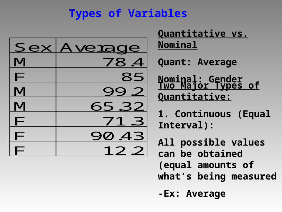
Sex AverageM 78.4F 85M 99.2M 65.32F 71.3F 90.43F 12.2

Types of Variables

Quantitative vs. Nominal

Quant: Average

Nominal: Gender

Two Major Types of Quantitative:

1. Continuous (Equal Interval):

All possible values can be obtained (equal amounts of what’s being measured

-Ex: Average

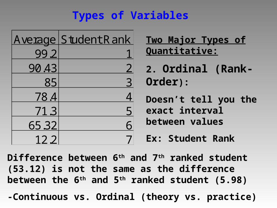
Average Student Rank99.2 1

90.43 285 3

78.4 471.3 5

65.32 612.2 7

Types of Variables

Two Major Types of Quantitative:

2. Ordinal (Rank-Order):

Doesn’t tell you the exact interval between values

Ex: Student Rank

Difference between 6th and 7th ranked student (53.12) is not the same as the difference between the 6th and 5th ranked student (5.98)

-Continuous vs. Ordinal (theory vs. practice)

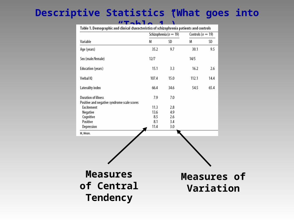
Descriptive Statistics (What goes into “Table 1”)

Measures of Central

Tendency

Measures of Variation

HEIGHT

75.072.570.067.565.062.560.0

Histogram

Fre

qu

en

cy16

14

12

10

8

6

4

2

0

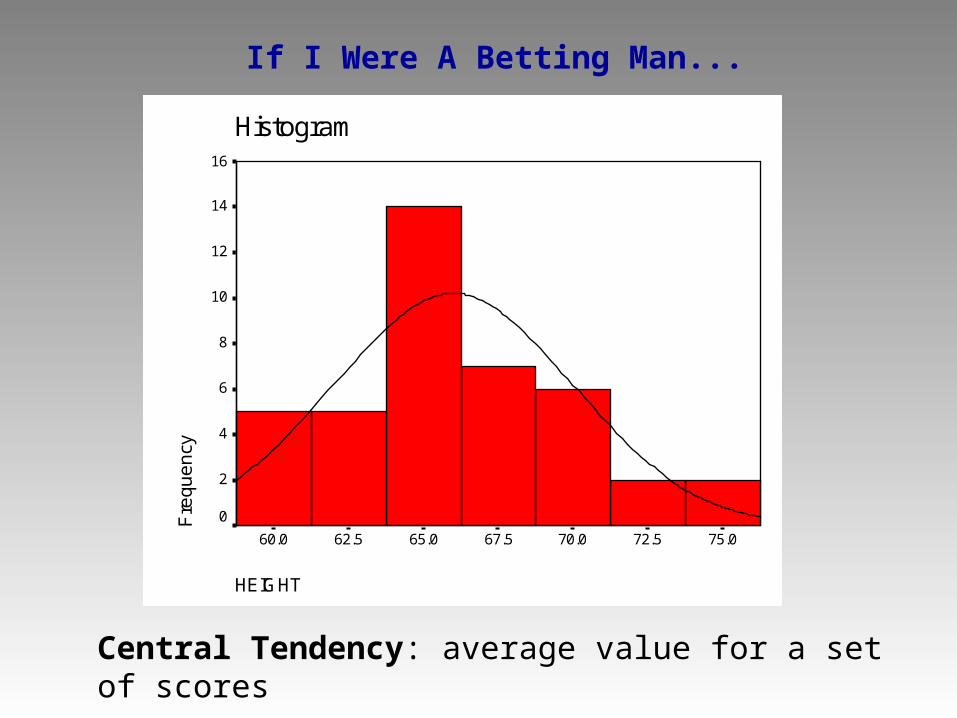
If I Were A Betting Man...

Central Tendency: average value for a set of scores

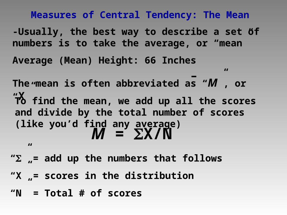
Measures of Central Tendency: The Mean

-Usually, the best way to describe a set of numbers is to take the average, or “mean”

Average (Mean) Height: 66 Inches

The mean is often abbreviated as “M”, or “X”

M = X/N

To find the mean, we add up all the scores and divide by the total number of scores (like you’d find any average)

“” = add up the numbers that follows

“X” = scores in the distribution

“N” = Total # of scores

686864657366715962636162657165

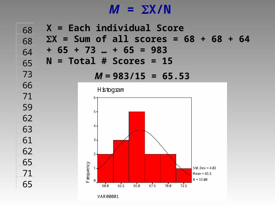
M = X/N

X = Each individual ScoreX = Sum of all scores = 68 + 68 + 64 + 65 + 73 … + 65 = 983N = Total # Scores = 15

M = 983/15 = 65.53

VAR00001

72.570.067.565.062.560.0

HistogramF

req

ue

ncy

6

5

4

3

2

1

0

Std. Dev = 4.02

Mean = 65.5

N = 15.00

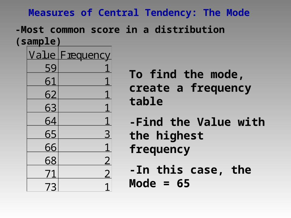
Measures of Central Tendency: The Mode

-Most common score in a distribution (sample)

Value Frequency59 161 162 163 164 165 366 168 271 273 1

To find the mode, create a frequency table

-Find the Value with the highest frequency

-In this case, the Mode = 65

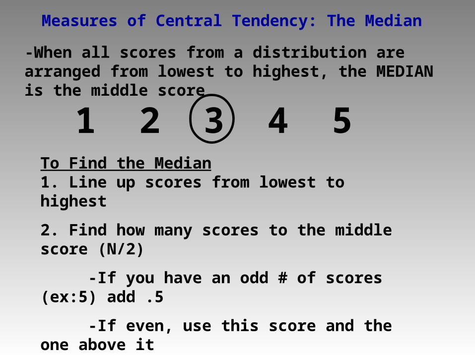
Measures of Central Tendency: The Median

-When all scores from a distribution are arranged from lowest to highest, the MEDIAN is the middle score

1 2 3 4 5To Find the Median1. Line up scores from lowest to highest

2. Find how many scores to the middle score (N/2)

-If you have an odd # of scores (ex:5) add .5

-If even, use this score and the one above it

3. If your N is odd, the middle score is the median, if your N is even the median is the average of the 2 middle scores

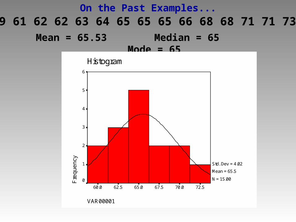
On the Past Examples...

Mean = 65.53 Median = 65 Mode = 65

VAR00001

72.570.067.565.062.560.0

Histogram

Fre

qu

en

cy6

5

4

3

2

1

0

Std. Dev = 4.02

Mean = 65.5

N = 15.00

59 61 62 62 63 64 65 65 65 66 68 68 71 71 73

59 61 62 62 63 64 65 65 65 66 68 68 71 71 73

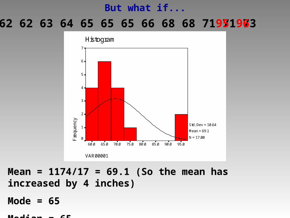
But what if...

VAR00001

95.090.085.080.075.070.065.060.0

Histogram

Fre

qu

en

cy

7

6

5

4

3

2

1

0

Std. Dev = 10.64

Mean = 69.1

N = 17.00

Mean = 1174/17 = 69.1 (So the mean has increased by 4 inches)

Mode = 65

Median = 65

95 96

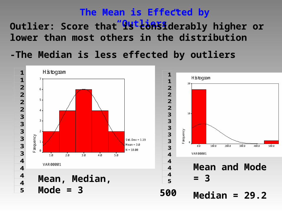
The Mean is Effected by “Outliers”

Outlier: Score that is considerably higher or lower than most others in the distribution

-The Median is less effected by outliers

VAR00001

5.04.03.02.01.0

Histogram

Fre

qu

en

cy

7

6

5

4

3

2

1

0

Std. Dev = 1.19

Mean = 3.0

N = 18.00

11222233333344445

Mean, Median, Mode = 3

11222233333344445

500

Mean and Mode = 3

Median = 29.2

VAR00001

500.0400.0300.0200.0100.00.0

Histogram

Fre

qu

en

cy

20

10

0

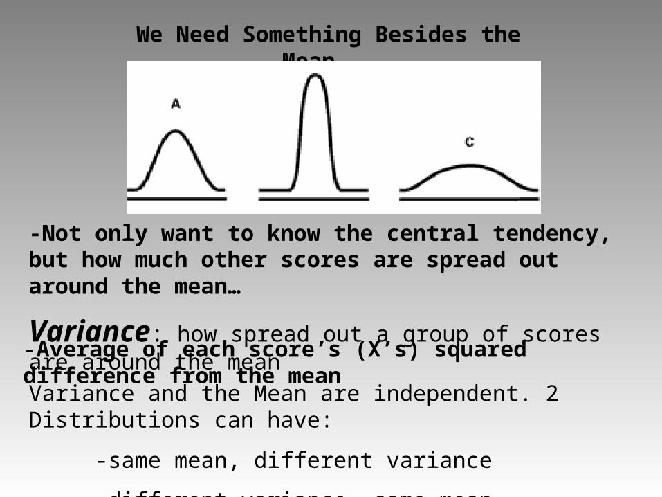
We Need Something Besides the Mean...

-Not only want to know the central tendency, but how much other scores are spread out around the mean…

Variance: how spread out a group of scores are around the mean

-Average of each score’s (X’s) squared difference from the mean

Variance and the Mean are independent. 2 Distributions can have:

-same mean, different variance

-different variance, same mean

Calculating Variance

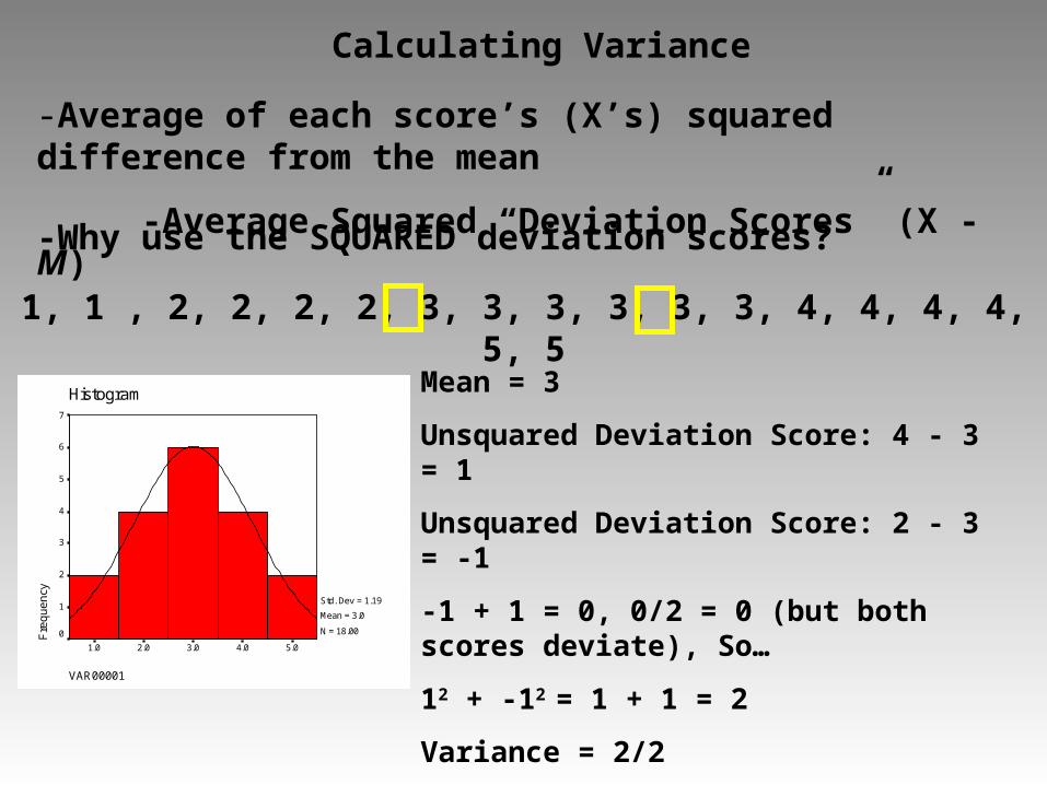
-Average of each score’s (X’s) squared difference from the mean

-Average Squared “Deviation Scores” (X - M)

-Why use the SQUARED deviation scores?

1, 1 , 2, 2, 2, 2, 3, 3, 3, 3, 3, 3, 4, 4, 4, 4, 5, 5

VAR00001

5.04.03.02.01.0

Histogram

Fre

qu

en

cy

7

6

5

4

3

2

1

0

Std. Dev = 1.19

Mean = 3.0

N = 18.00

Mean = 3

Unsquared Deviation Score: 4 - 3 = 1

Unsquared Deviation Score: 2 - 3 = -1

-1 + 1 = 0, 0/2 = 0 (but both scores deviate), So…

12 + -12 = 1 + 1 = 2

Variance = 2/2

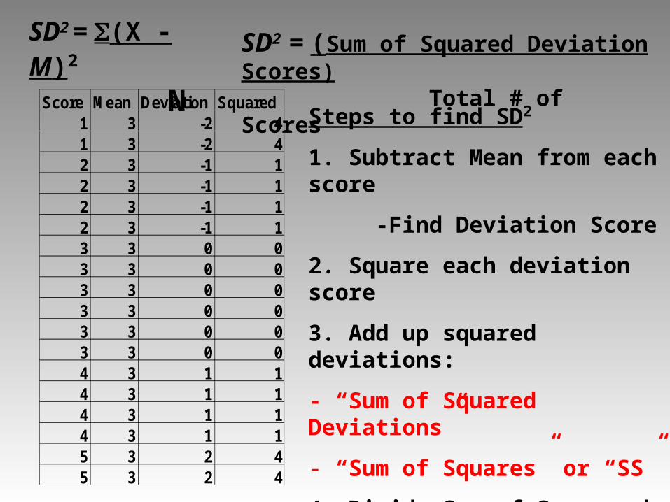
SD2 = (X - M)2

NSD2 = (Sum of Squared Deviation Scores)

Total # of ScoresScore Mean Deviation Squared

1 3 -2 41 3 -2 42 3 -1 12 3 -1 12 3 -1 12 3 -1 13 3 0 03 3 0 03 3 0 03 3 0 03 3 0 03 3 0 04 3 1 14 3 1 14 3 1 14 3 1 15 3 2 45 3 2 4

Steps to find SD2

1. Subtract Mean from each score

-Find Deviation Score

2. Square each deviation score

3. Add up squared deviations:

- “Sum of Squared Deviations”

- “Sum of Squares” or “SS”

4. Divide Sum of Squares by N (Total # of Scores)

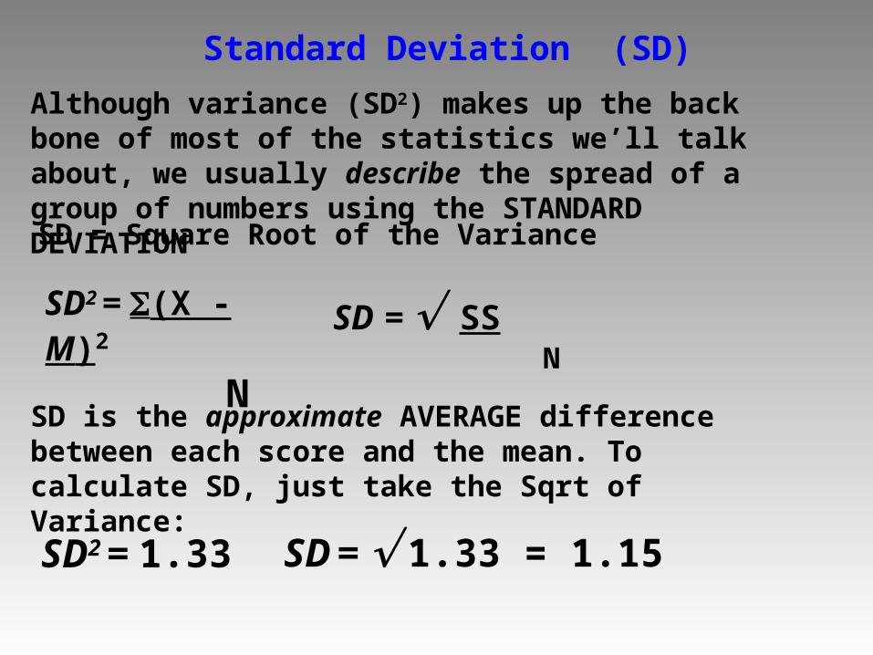
Standard Deviation (SD)

Although variance (SD2) makes up the back bone of most of the statistics we’ll talk about, we usually describe the spread of a group of numbers using the STANDARD DEVIATION

SD = Square Root of the Variance

SD2 = (X - M)2

NSD = SS

N

SD is the approximate AVERAGE difference between each score and the mean. To calculate SD, just take the Sqrt of Variance:

SD2 = 1.33 SD = 1.33 = 1.15

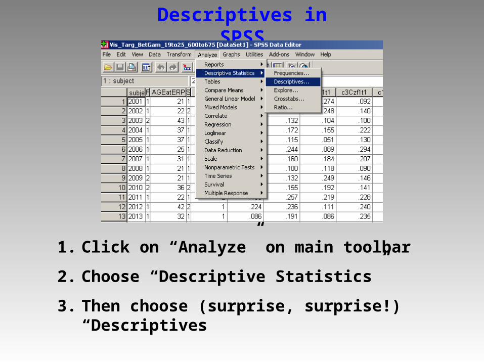
Descriptives in SPSS

1. Click on “Analyze” on main toolbar

2. Choose “Descriptive Statistics”

3. Then choose (surprise, surprise!) “Descriptives

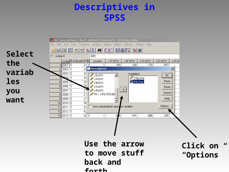
Descriptives in SPSS

Select the variables you want

Use the arrow to move stuff back and forth…

Click on “Options”

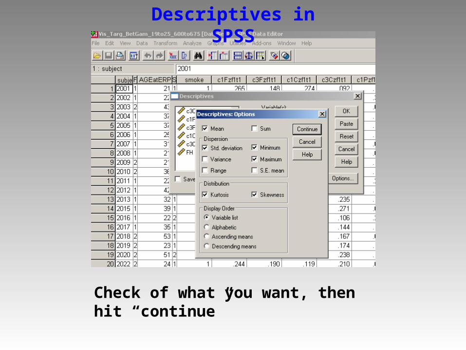
Descriptives in SPSS

Check of what you want, then hit “continue”

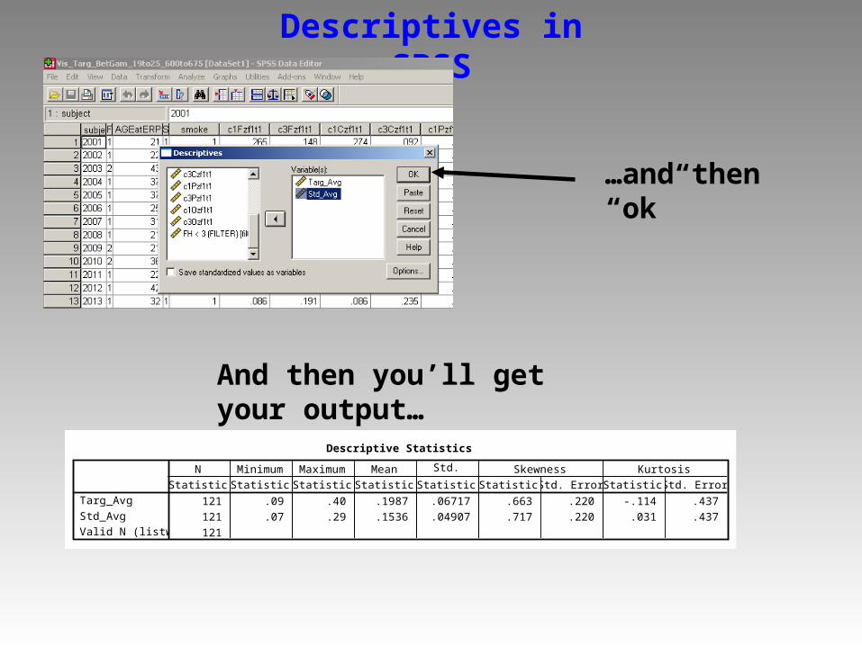
Descriptives in SPSS

…and then “ok”

Descriptive Statistics

121 .09 .40 .1987 .06717 .663 .220 -.114 .437

121 .07 .29 .1536 .04907 .717 .220 .031 .437

121

Targ_Avg

Std_Avg

Valid N (listwise)

Statistic Statistic Statistic Statistic Statistic Statistic Std. Error Statistic Std. Error

N Minimum Maximum Mean Std.Deviation

Skewness Kurtosis

And then you’ll get your output…

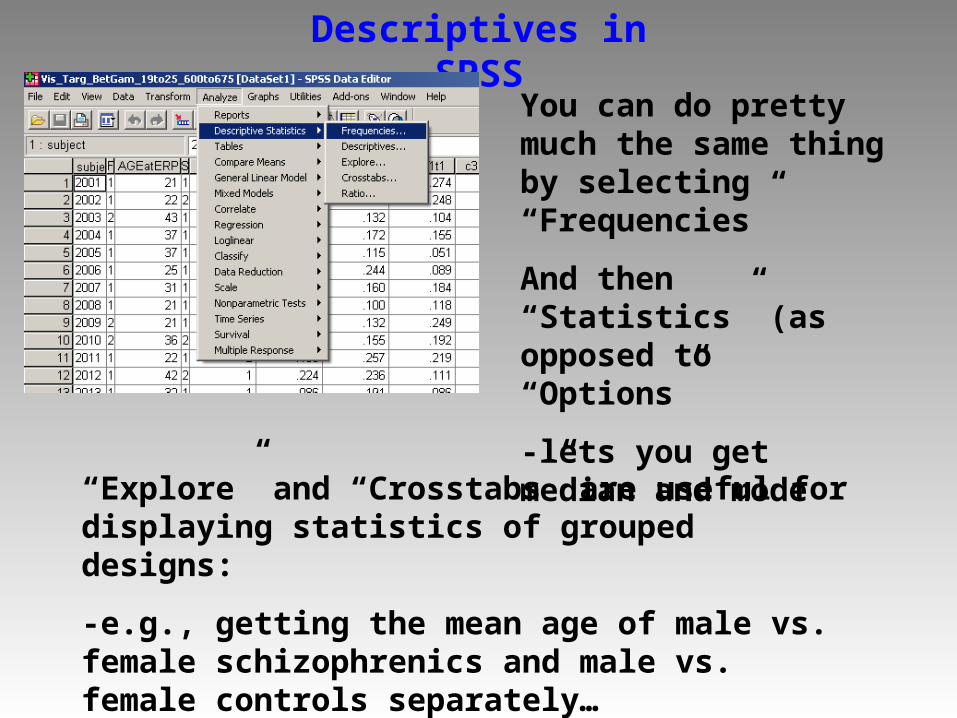
Descriptives in SPSS

You can do pretty much the same thing by selecting “Frequencies”

And then “Statistics” (as opposed to “Options”

-lets you get median and mode

“Explore” and “Crosstabs” are useful for displaying statistics of grouped designs:

-e.g., getting the mean age of male vs. female schizophrenics and male vs. female controls separately…

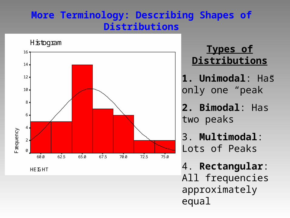
More Terminology: Describing Shapes of Distributions

HEIGHT

75.072.570.067.565.062.560.0

Histogram

Fre

qu

en

cy

16

14

12

10

8

6

4

2

0

Types of Distributions

1. Unimodal: Has only one “peak”

2. Bimodal: Has two peaks

3. Multimodal: Lots of Peaks

4. Rectangular: All frequencies approximately equal

Unimodal Distribution Bimodal Distribution

Multimodal Rectangular

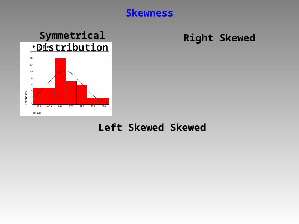
Skewness

HEIGHT

75.072.570.067.565.062.560.0

Histogram

Fre

qu

en

cy

16

14

12

10

8

6

4

2

0

Symmetrical Distribution Right Skewed

Left Skewed Skewed

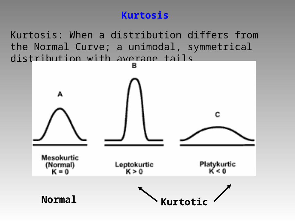
Kurtosis

Kurtosis: When a distribution differs from the Normal Curve; a unimodal, symmetrical distribution with average tails

Normal Kurtotic

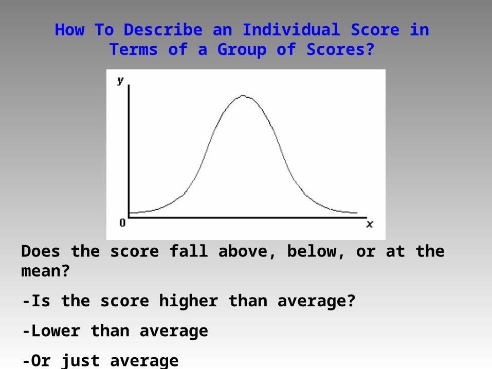
How To Describe an Individual Score in Terms of a Group of Scores?

Does the score fall above, below, or at the mean?

-Is the score higher than average?

-Lower than average

-Or just average

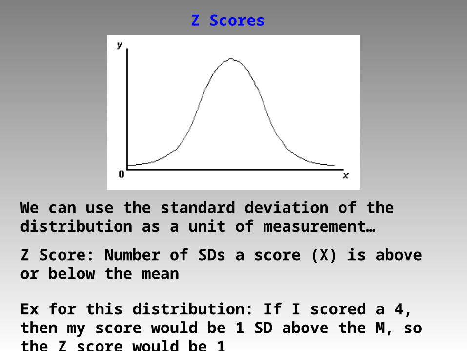
Z Scores

We can use the standard deviation of the distribution as a unit of measurement…

Z Score: Number of SDs a score (X) is above or below the mean

Ex for this distribution: If I scored a 4, then my score would be 1 SD above the M, so the Z score would be 1

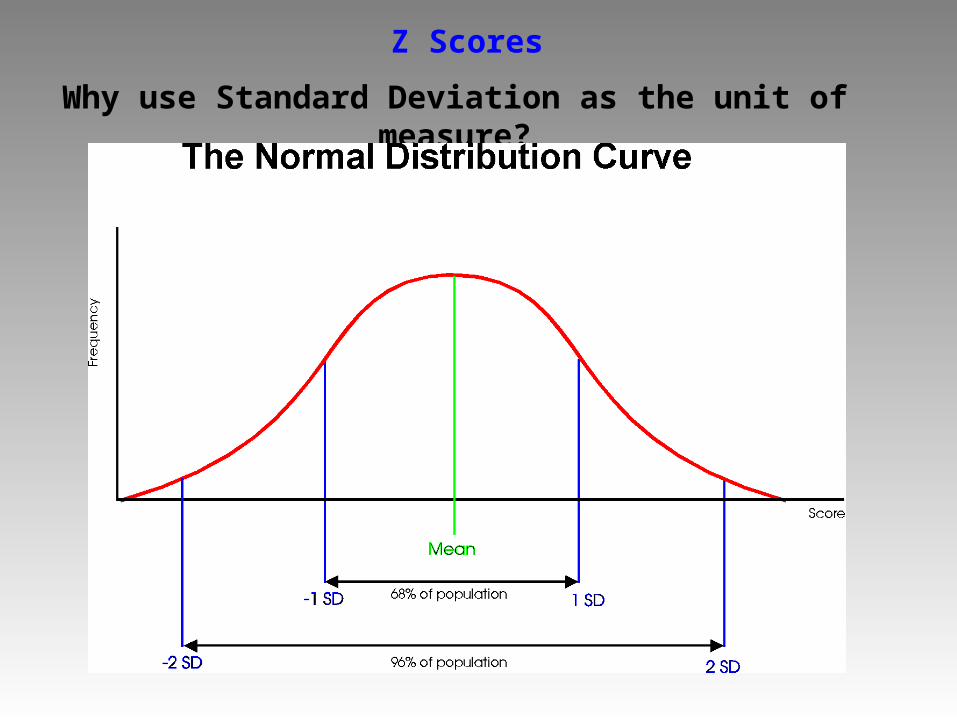
Z Scores

Why use Standard Deviation as the unit of measure?

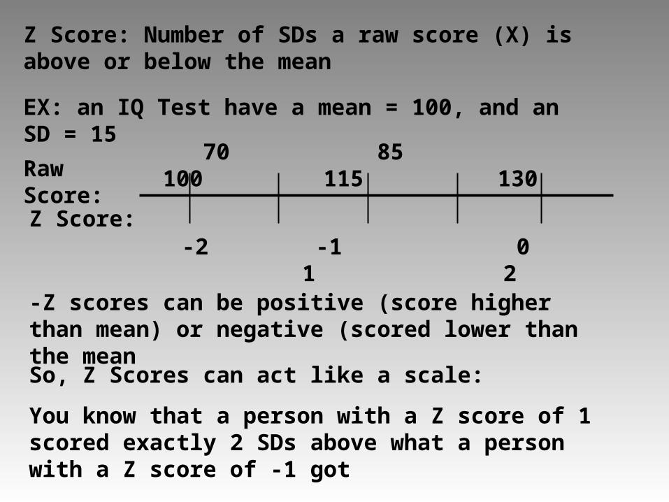
Z Score: Number of SDs a raw score (X) is above or below the mean

EX: an IQ Test have a mean = 100, and an SD = 15

Raw Score:

Z Score:

70 85 100 115 130

-2 -1 0 1 2

So, Z Scores can act like a scale:

You know that a person with a Z score of 1 scored exactly 2 SDs above what a person with a Z score of -1 got

-Z scores can be positive (score higher than mean) or negative (scored lower than the mean

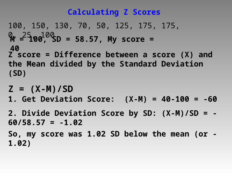
Calculating Z Scores

100, 150, 130, 70, 50, 125, 175, 175, 0, 25, 100

M = 100, SD = 58.57, My score = 40

Z score = Difference between a score (X) and the Mean divided by the Standard Deviation (SD)

Z = (X-M)/SD

1. Get Deviation Score: (X-M) = 40-100 = -60

2. Divide Deviation Score by SD: (X-M)/SD = -60/58.57 = -1.02

So, my score was 1.02 SD below the mean (or -1.02)

You Can Use Z scores to compare scores taken from 2 Different Distributions (Different Variables)

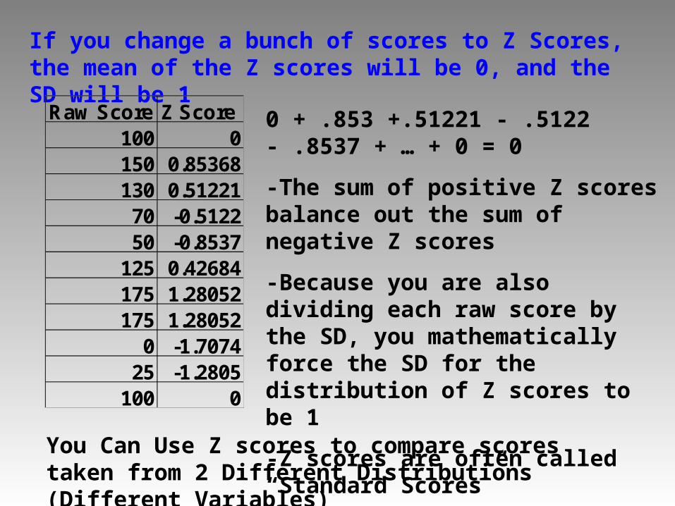
If you change a bunch of scores to Z Scores, the mean of the Z scores will be 0, and the SD will be 1

Raw Score Z Score100 0150 0.85368130 0.5122170 -0.512250 -0.8537

125 0.42684175 1.28052175 1.28052

0 -1.707425 -1.2805

100 0

0 + .853 +.51221 - .5122 - .8537 + … + 0 = 0

-The sum of positive Z scores balance out the sum of negative Z scores

-Because you are also dividing each raw score by the SD, you mathematically force the SD for the distribution of Z scores to be 1

-Z scores are often called “Standard Scores”

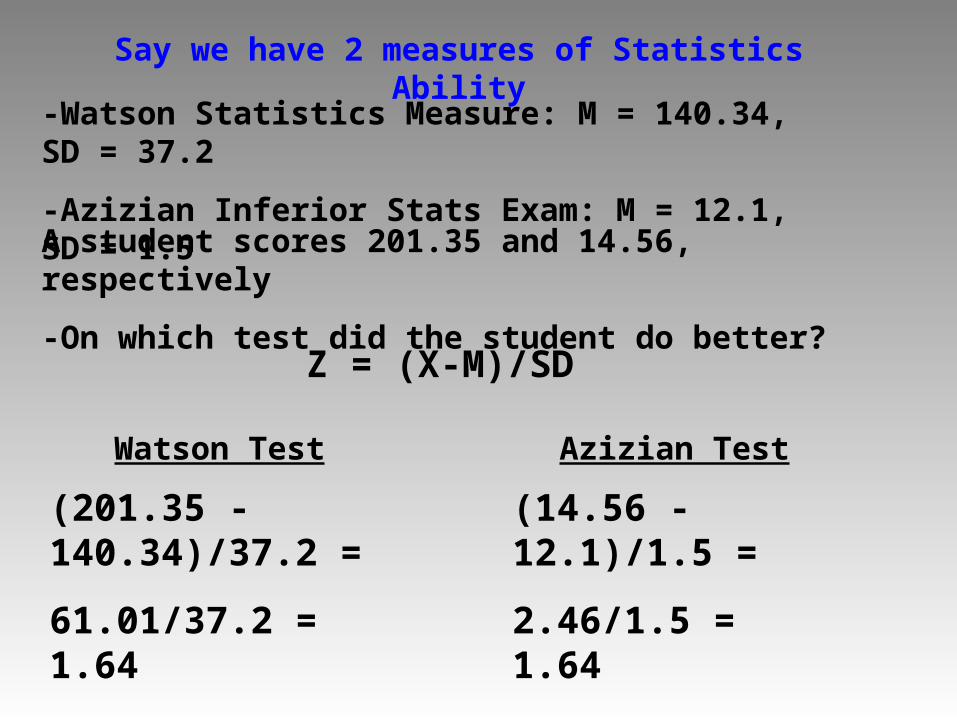
Say we have 2 measures of Statistics Ability

-Watson Statistics Measure: M = 140.34, SD = 37.2

-Azizian Inferior Stats Exam: M = 12.1, SD = 1.5

A student scores 201.35 and 14.56, respectively

-On which test did the student do better?

Z = (X-M)/SD

Watson Test Azizian Test

(201.35 - 140.34)/37.2 =

61.01/37.2 = 1.64

Z = 1.64

(14.56 - 12.1)/1.5 =

2.46/1.5 = 1.64

Z = 1.64

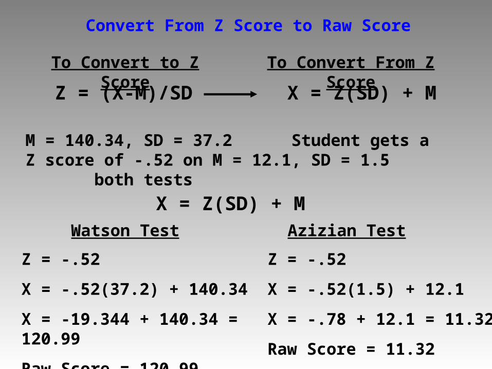
Convert From Z Score to Raw Score

Z = (X-M)/SD

To Convert to Z Score To Convert From Z Score

X = Z(SD) + M

M = 140.34, SD = 37.2 Student gets a Z score of -.52 on M = 12.1, SD = 1.5 both tests

X = Z(SD) + MWatson Test Azizian Test

Z = -.52

X = -.52(37.2) + 140.34

X = -19.344 + 140.34 = 120.99

Raw Score = 120.99

Z = -.52

X = -.52(1.5) + 12.1

X = -.78 + 12.1 = 11.32

Raw Score = 11.32