Stature and Status: Height, Ability, and Labor Market Outcomesaccase/downloads/Stature_and_Status.pdfStature and Status: Height, Ability, and Labor Market Outcomes Anne Case and Christina

499

[ Journal of Political Economy, 2008, vol. 116, no. 3]� 2008 by The University of Chicago. All rights reserved. 0022-3808/2008/11603-0003$10.00

Stature and Status: Height, Ability, and Labor

Market Outcomes

Anne Case and Christina PaxsonPrinceton University

The well-known association between height and earnings is oftenthought to reflect factors such as self-esteem, social dominance, anddiscrimination. We offer a simpler explanation: height is positivelyassociated with cognitive ability, which is rewarded in the labor market.Using data from the United States and the United Kingdom, we showthat taller children have higher average cognitive test scores and thatthese test scores explain a large portion of the height premium inearnings. Children who have higher test scores also experience earlieradolescent growth spurts, so that height in adolescence serves as amarker of cognitive ability.

I. Introduction

It has long been recognized that taller adults hold jobs of higher statusand, on average, earn more than other workers. Empirical research onheight and success in the U.S. labor market dates back at least a century.Gowin (1915), for example, presents survey evidence documenting thedifference in the distributions of heights of executives and of “averagemen.” Gowin also compares the heights of persons of differing statusin the same profession, finding that bishops are taller on average thanpreachers in small towns, and sales managers are taller than salesmen,with similar results for lawyers, teachers, and railroad employees (32).

We thank Tom Vogl and Mahnaz Islam for expert research assistance, Angus Deatonfor comments on an earlier draft, and two anonymous referees for useful comments. Thisresearch has been supported by grant HD041141 from the National Institute of ChildHealth and Human Development and grant P01 AG005842 from the National Instituteon Aging.

500 journal of political economy

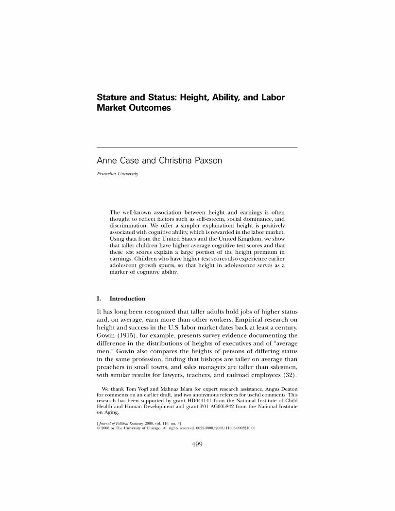
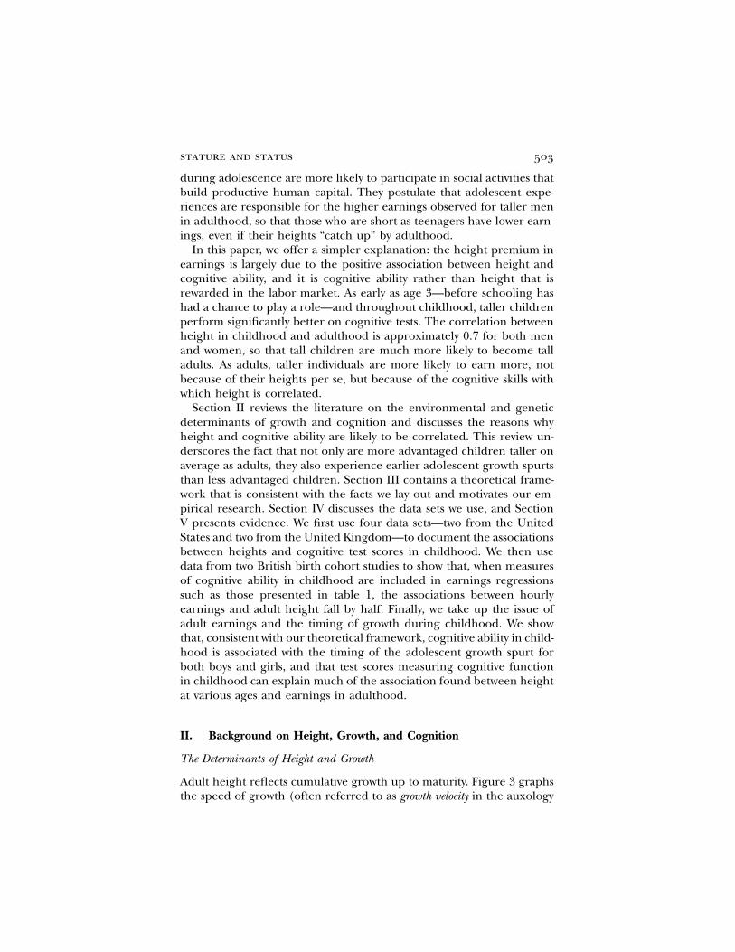
Height continues to be highly correlated with labor market successin developed countries. Figure 1 provides evidence from the UnitedStates and the United Kingdom that more highly skilled jobs attracttaller workers. American men in white-collar occupations are an inchtaller, on average, than men in blue-collar occupations. Among 30-year-old men in the United Kingdom, those working in professional andmanagerial occupations are 0.6 inch taller on average than those inmanual occupations. Results for women are quite similar: in the UnitedKingdom, women working as professionals and managers are an inchtaller on average than those in manual unskilled occupations.

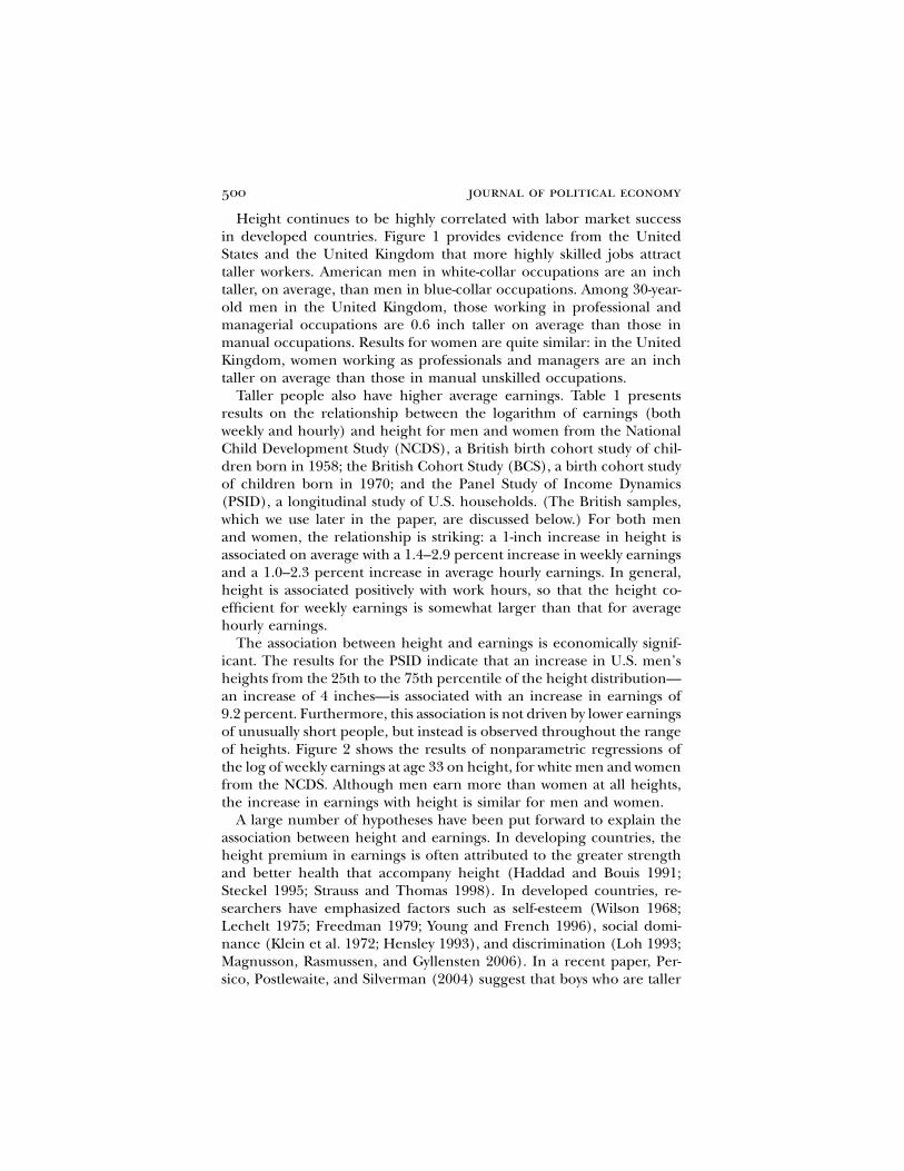
Taller people also have higher average earnings. Table 1 presentsresults on the relationship between the logarithm of earnings (bothweekly and hourly) and height for men and women from the NationalChild Development Study (NCDS), a British birth cohort study of chil-dren born in 1958; the British Cohort Study (BCS), a birth cohort studyof children born in 1970; and the Panel Study of Income Dynamics(PSID), a longitudinal study of U.S. households. (The British samples,which we use later in the paper, are discussed below.) For both menand women, the relationship is striking: a 1-inch increase in height isassociated on average with a 1.4–2.9 percent increase in weekly earningsand a 1.0–2.3 percent increase in average hourly earnings. In general,height is associated positively with work hours, so that the height co-efficient for weekly earnings is somewhat larger than that for averagehourly earnings.

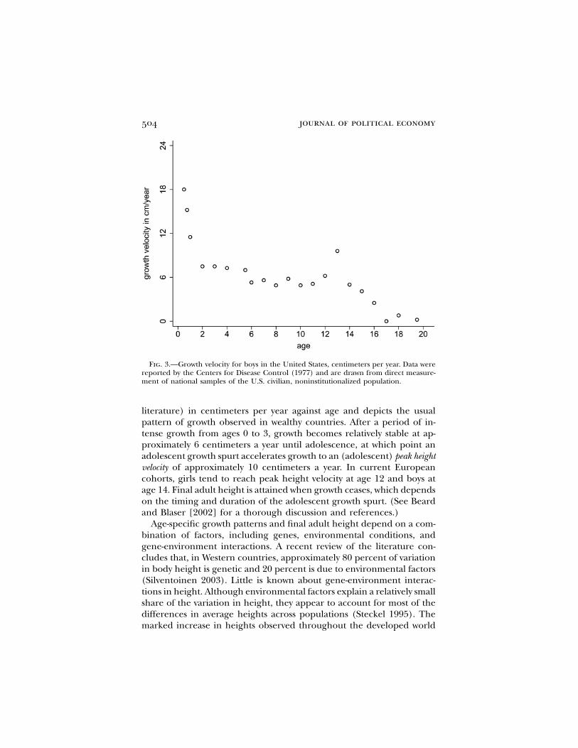
The association between height and earnings is economically signif-icant. The results for the PSID indicate that an increase in U.S. men’sheights from the 25th to the 75th percentile of the height distribution—an increase of 4 inches—is associated with an increase in earnings of9.2 percent. Furthermore, this association is not driven by lower earningsof unusually short people, but instead is observed throughout the rangeof heights. Figure 2 shows the results of nonparametric regressions ofthe log of weekly earnings at age 33 on height, for white men and womenfrom the NCDS. Although men earn more than women at all heights,the increase in earnings with height is similar for men and women.

A large number of hypotheses have been put forward to explain theassociation between height and earnings. In developing countries, theheight premium in earnings is often attributed to the greater strengthand better health that accompany height (Haddad and Bouis 1991;Steckel 1995; Strauss and Thomas 1998). In developed countries, re-searchers have emphasized factors such as self-esteem (Wilson 1968;Lechelt 1975; Freedman 1979; Young and French 1996), social domi-nance (Klein et al. 1972; Hensley 1993), and discrimination (Loh 1993;Magnusson, Rasmussen, and Gyllensten 2006). In a recent paper, Per-sico, Postlewaite, and Silverman (2004) suggest that boys who are taller

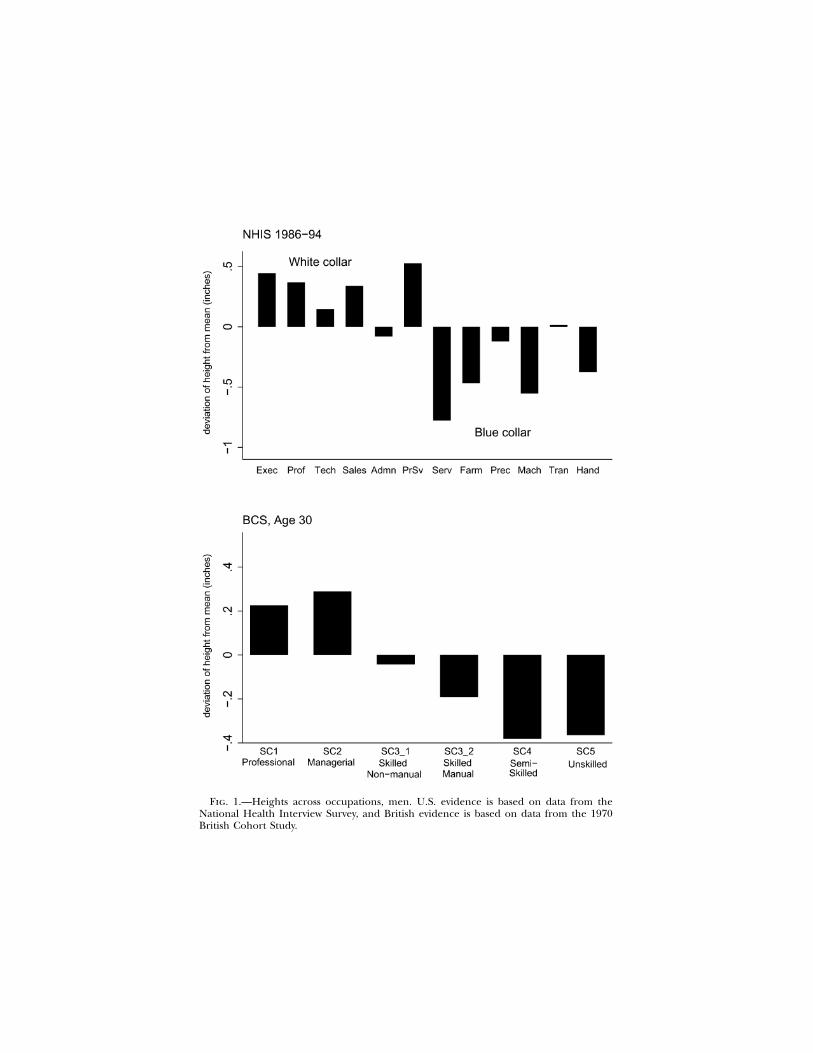
Fig. 1.—Heights across occupations, men. U.S. evidence is based on data from theNational Health Interview Survey, and British evidence is based on data from the 1970British Cohort Study.

TABLE 1Log Earnings and Height

Dependent Variable

Men Women

HeightCoefficient Observations

HeightCoefficient Observations

A. NCDS

Log weekly grossearnings

.026(.004)

4,927 .024(.007)

5,033

Log average hourlygross earnings

.023(.004)

4,860 .019(.005)

4,995

B. BCS

Log weekly grossearnings

.014(.003)

2,265 .029(.006)

2,136

Log average hourlygross earnings

.010(.003)

2,253 .015(.004)

2,127

C. PSID

Log weekly earnings .023(.004)

23,465 .014(.006)

21,271

Log average hourlyearnings

.019(.004)

23,465 .012(.003)

21,271

Note.—Ordinary least squares (OLS) regression coefficients reported for height in inches, with standard errors inparentheses. The NCDS and PSID regressions use multiple observations per person, and unobservables are clusteredat the individual level. The NCDS and BCS samples are restricted to those for whom we have test scores at ages 7 and11 (NCDS) or 5 and 10 (BCS). The PSID sample consists of white household heads or wives between the ages of 25and 60, inclusive, between 1988 and 1997. NCDS and BCS regressions include indicators for ethnicity, and the NCDSregressions also include an age indicator. The PSID regressions include a set of age and year indicators.

Fig. 2.—Log earnings and height, men and women

stature and status 503

during adolescence are more likely to participate in social activities thatbuild productive human capital. They postulate that adolescent expe-riences are responsible for the higher earnings observed for taller menin adulthood, so that those who are short as teenagers have lower earn-ings, even if their heights “catch up” by adulthood.

In this paper, we offer a simpler explanation: the height premium inearnings is largely due to the positive association between height andcognitive ability, and it is cognitive ability rather than height that isrewarded in the labor market. As early as age 3—before schooling hashad a chance to play a role—and throughout childhood, taller childrenperform significantly better on cognitive tests. The correlation betweenheight in childhood and adulthood is approximately 0.7 for both menand women, so that tall children are much more likely to become talladults. As adults, taller individuals are more likely to earn more, notbecause of their heights per se, but because of the cognitive skills withwhich height is correlated.

Section II reviews the literature on the environmental and geneticdeterminants of growth and cognition and discusses the reasons whyheight and cognitive ability are likely to be correlated. This review un-derscores the fact that not only are more advantaged children taller onaverage as adults, they also experience earlier adolescent growth spurtsthan less advantaged children. Section III contains a theoretical frame-work that is consistent with the facts we lay out and motivates our em-pirical research. Section IV discusses the data sets we use, and SectionV presents evidence. We first use four data sets—two from the UnitedStates and two from the United Kingdom—to document the associationsbetween heights and cognitive test scores in childhood. We then usedata from two British birth cohort studies to show that, when measuresof cognitive ability in childhood are included in earnings regressionssuch as those presented in table 1, the associations between hourlyearnings and adult height fall by half. Finally, we take up the issue ofadult earnings and the timing of growth during childhood. We showthat, consistent with our theoretical framework, cognitive ability in child-hood is associated with the timing of the adolescent growth spurt forboth boys and girls, and that test scores measuring cognitive functionin childhood can explain much of the association found between heightat various ages and earnings in adulthood.

II. Background on Height, Growth, and Cognition

The Determinants of Height and Growth

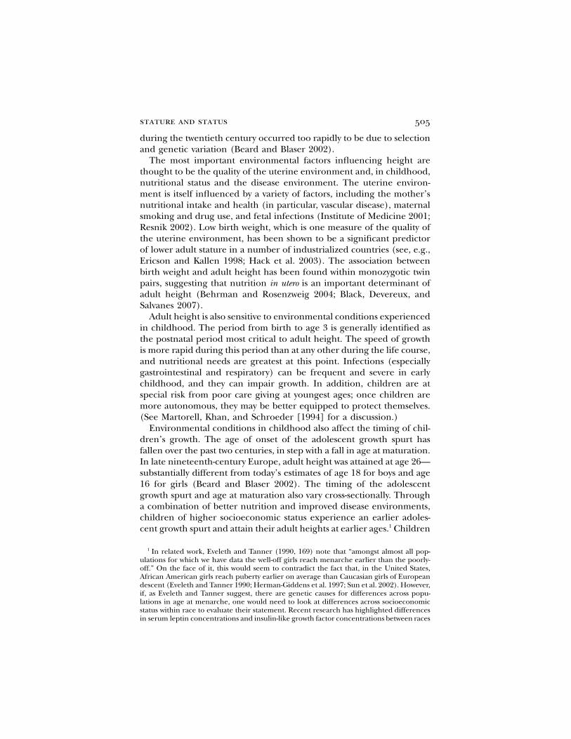
Adult height reflects cumulative growth up to maturity. Figure 3 graphsthe speed of growth (often referred to as growth velocity in the auxology


Fig. 3.—Growth velocity for boys in the United States, centimeters per year. Data werereported by the Centers for Disease Control (1977) and are drawn from direct measure-ment of national samples of the U.S. civilian, noninstitutionalized population.

literature) in centimeters per year against age and depicts the usualpattern of growth observed in wealthy countries. After a period of in-tense growth from ages 0 to 3, growth becomes relatively stable at ap-proximately 6 centimeters a year until adolescence, at which point anadolescent growth spurt accelerates growth to an (adolescent) peak heightvelocity of approximately 10 centimeters a year. In current Europeancohorts, girls tend to reach peak height velocity at age 12 and boys atage 14. Final adult height is attained when growth ceases, which dependson the timing and duration of the adolescent growth spurt. (See Beardand Blaser [2002] for a thorough discussion and references.)

Age-specific growth patterns and final adult height depend on a com-bination of factors, including genes, environmental conditions, andgene-environment interactions. A recent review of the literature con-cludes that, in Western countries, approximately 80 percent of variationin body height is genetic and 20 percent is due to environmental factors(Silventoinen 2003). Little is known about gene-environment interac-tions in height. Although environmental factors explain a relatively smallshare of the variation in height, they appear to account for most of thedifferences in average heights across populations (Steckel 1995). Themarked increase in heights observed throughout the developed world


during the twentieth century occurred too rapidly to be due to selectionand genetic variation (Beard and Blaser 2002).

The most important environmental factors influencing height arethought to be the quality of the uterine environment and, in childhood,nutritional status and the disease environment. The uterine environ-ment is itself influenced by a variety of factors, including the mother’snutritional intake and health (in particular, vascular disease), maternalsmoking and drug use, and fetal infections (Institute of Medicine 2001;Resnik 2002). Low birth weight, which is one measure of the quality ofthe uterine environment, has been shown to be a significant predictorof lower adult stature in a number of industrialized countries (see, e.g.,Ericson and Kallen 1998; Hack et al. 2003). The association betweenbirth weight and adult height has been found within monozygotic twinpairs, suggesting that nutrition in utero is an important determinant ofadult height (Behrman and Rosenzweig 2004; Black, Devereux, andSalvanes 2007).

Adult height is also sensitive to environmental conditions experiencedin childhood. The period from birth to age 3 is generally identified asthe postnatal period most critical to adult height. The speed of growthis more rapid during this period than at any other during the life course,and nutritional needs are greatest at this point. Infections (especiallygastrointestinal and respiratory) can be frequent and severe in earlychildhood, and they can impair growth. In addition, children are atspecial risk from poor care giving at youngest ages; once children aremore autonomous, they may be better equipped to protect themselves.(See Martorell, Khan, and Schroeder [1994] for a discussion.)

Environmental conditions in childhood also affect the timing of chil-dren’s growth. The age of onset of the adolescent growth spurt hasfallen over the past two centuries, in step with a fall in age at maturation.In late nineteenth-century Europe, adult height was attained at age 26—substantially different from today’s estimates of age 18 for boys and age16 for girls (Beard and Blaser 2002). The timing of the adolescentgrowth spurt and age at maturation also vary cross-sectionally. Througha combination of better nutrition and improved disease environments,children of higher socioeconomic status experience an earlier adoles-cent growth spurt and attain their adult heights at earlier ages.1 Children

1 In related work, Eveleth and Tanner (1990, 169) note that “amongst almost all pop-ulations for which we have data the well-off girls reach menarche earlier than the poorly-off.” On the face of it, this would seem to contradict the fact that, in the United States,African American girls reach puberty earlier on average than Caucasian girls of Europeandescent (Eveleth and Tanner 1990; Herman-Giddens et al. 1997; Sun et al. 2002). However,if, as Eveleth and Tanner suggest, there are genetic causes for differences across popu-lations in age at menarche, one would need to look at differences across socioeconomicstatus within race to evaluate their statement. Recent research has highlighted differencesin serum leptin concentrations and insulin-like growth factor concentrations between races


who experience deprivation may experience an extension of the growthperiod that can last several years (Steckel 1995). An extended adolescentgrowth spurt can help shorter children gain a similar amount of heightas other children do during adolescence, but on average this does noterase height deficits that developed in early childhood (Satyanarayanaet al. 1989; Martorell, Rivera, and Kaplowitz 1990; Martorell et al. 1994;Hack et al. 2003).

Differences in the timing of pubertal growth spurts act to temporarilymagnify differences in heights between economic classes during ado-lescence. This has long been true: data collected at a boarding schoolin Germany in the eighteenth century, for example, suggest that upper-class boys reached their peak height velocity a full year earlier thanlower-class boys, exaggerating the height difference between them dur-ing their teen years (Komlos et al. 1992). When the authors control foryear and region of birth, height differences between sons of low aris-tocrats and middle-class boys grew from 2.4 centimeters at age 10 to 5.8centimeters at age 15, before returning to a mean height difference of2.1 centimeters at age 19.

Height and Cognitive Ability

The positive association between height and IQ has been documentedin studies going back at least a century (Tanner 1979). However, themechanisms that underlie this relationship are still not well understood.The existing evidence on channels linking height and cognitive abilitycomes from medical research; sibling and twin studies; studies of shocksto the early-life environment, which offer the possibility of examiningoutcomes through the lens of natural experiments; and observationalstudies.

Biological channels have been identified that may influence bothheight and cognition over a broad range of the population.2 Insulin-like growth factors affect body growth while also influencing areas ofthe brain in which cognition occurs (Berger 2001). Similarly, thyroidhormone stimulates growth and at the same time influences neuraldevelopment (Richards et al. 2002). It is unclear, however, precisely howgenetic and environmental factors interact in operating these biologicalchannels.3

as possible reasons for earlier menarche among African Americans (Wong et al. 1998,1999).

2 Several rare genetic disorders also result in both short stature and cognitive impair-ment. Turner’s syndrome, e.g., is an X-linked genetic disorder that affects stature andsome aspects of cognitive development in girls.

3 See Brown and Demmer (2002) for a discussion of the role of gene-environmentinteractions in the context of congenital hypothyroidism.


Evidence on the role of genetics in explaining the correlation betweenheight and intelligence comes from a number of twin studies. Sundetet al. (2005) use differences in cross-trait (height and intelligence),cross-twin correlations between monozygotic (MZ) and dizygotic (DZ)twin pairs to identify the roles played by shared environments and sharedgenes. They conclude that the environment plays a large role and isresponsible for 65 percent of the height-intelligence correlation, withgenes responsible for 35 percent of the observed correlation. Theseauthors report that their results are very similar to those on cross-trait,cross-twin correlations found much earlier by Husen (1959) in a largestudy of MZ and DZ twin pairs.

Twin studies also shed light on the role played by nutrition in uteroas a determinant of both adult height and IQ. Black et al. (2007) ex-amine data on male twin pairs born in Norway between 1967 and 1987,noting that the difference in the twins’ birth weights is largely due tonutritional intake in utero. They find that, on average, the twin bornat the higher birth weight is significantly taller in adulthood and scoressignificantly higher on IQ tests. Similarly, using data from the MinnesotaTwin Registry and an MZ fixed-effect framework, Behrman and Rosen-zweig (2004) find fetal growth (birth weight divided by gestation) to besignificantly associated with height and years of completed schooling inadulthood.

Almond (2006) uses the arrival of the 1918 influenza pandemic as anatural experiment with which to gauge the long-run consequences ofprenatal exposure to the flu. He finds that individuals who were exposedduring gestation had lower educational attainment and poorer healthin adulthood than individuals born prior to the outbreak or conceivedafter the pandemic ended.4

Nutrition in infancy and childhood may also affect cognitive abilityas well as height, producing a correlation between the two (Lynn 1989;Kretchmer, Beard, and Carlson 1996). Several randomized experimentssupport this idea. One found that nutritional supplements given togrowth-retarded children improved their cognitive test scores, althoughthese gains dissipated after the supplementation ended (Grantham-McGregor 2002). A follow-up to the Guatemalan INCAP (Instituto deNutricion de Centroamerica y Panama) study, which provided children

4 Although Almond does not assess height or cognitive function, his findings for edu-cational attainment and health in adulthood suggest that the channel from prenatal healthto adult outcomes may provide another link between height and cognition. A related linkmay occur through inflammation. Crimmins and Finch (2006) argue that an inflammatoryresponse to infection can inhibit growth. In particular, they note that “if infection occursduring development, substantial energy is reallocated at the expense of growth, as requiredby the body for immune defense reactions and for repair” (500). Inflammation is alsothought to have lasting effects on cognitive function (Holding and Snow 2001; Ekdahl etal. 2003).


with nutrition supplements, found long-term effects on the heights ofchildren who received the treatment during the first 3 years of life andgains in (some) cognitive test scores and educational attainment (Mar-torell et al. 2005). Although these studies are intriguing, it should benoted that both were conducted in very impoverished environments.There is little direct evidence on how childhood nutrition influencescognitive development in wealthier settings.

Observational studies suggest that an additional link between heightand cognition may work through maternal smoking during pregnancy,which is associated with slower fetal growth, as well as lower cognitivetest scores, behavioral problems, and attention deficit hyperactivity dis-order (Weitzman, Gortmaker, and Sobol 1992; Romano et al. 2006).While these outcomes may be the result of factors correlated withmother’s smoking during pregnancy rather than the direct effect ofsmoking, animal studies have documented the role of prenatal nicotineexposure on neural development (Slotkin 1998).

III. Empirical Framework

We develop a statistical model in which both cognitive ability and heightat different ages are influenced by an unobserved factor that reflectsthe combined effects of environmental conditions (such as health andnutrition), biological factors, genetic factors, and gene-environment in-teractions. We refer to the unobserved factor as an individual’s endow-ment. For our purposes, it is not necessary to distinguish the geneticand environmental factors that determine this endowment.5 To the ex-tent that they reflect genetic inheritance, or gene-environment inter-actions in utero, endowments would be fixed at birth. However, as dis-cussed above, early-life environment is also critical to physical andcognitive development, and the only assumption we need in order tokeep the model simple is that endowments are set prior to the childhoodmeasurements we have for height and cognitive function.

We use the model to derive testable implications for the relationshipsbetween wages, cognitive ability, and heights in both childhood andadulthood. We assume that cognitive ability c is a linear function of theendowment n. Assuming that all variables have been centered aroundtheir means, we have

c p ln � u, (1)

where n is defined so that l is positive. Heights at each age, from

5 Understanding the extent to which this endowment can be influenced by prenatalcare and early-life environment is of great importance for social policy. Unfortunately, wedo not currently have access to data that would allow us to address this.


childhood to early adulthood, are also assumed to be linear functionsof the endowment. After heights at each age are centered around theirmeans, height at age i is expressed as

h p a n � v , i p 1, … , K, (2)i i i

where refers to final adult height. Although we expect to be positiveh aK i

for each age, this parameter is not necessarily the same for all ages. Theliterature discussed above indicates that may be larger during theai

years of the adolescent growth spurt than in middle childhood or inadulthood. It may also be large in early childhood, when height reflectsprenatal conditions and early childhood health and nutrition.

For simplicity, we assume that the wage in adulthood is a function ofcognitive ability alone and is not a function of height:

w p bc � e. (3)

We also assume that the unobserved endowment is the only factor thatproduces correlations between cognitive ability, heights, and wages, sothat the covariances between all error terms in (1), (2), and (3) arezero. The variance of is denoted as and the variance of n is .2 2v j ji i n

Given this framework, a regression of the wage on height at any singleage will yield a positive coefficient. Specifically, the coefficient on ,hi

when it is the only height measure included in the wage regression, willhave a probability limit of

1p lim b p bla . (4)i i 2 2 2[ ]a � (j /j )i i n

In words, the coefficient on height in the wage regression reflects theassociation between height and cognitive ability that works through theunobserved endowment n. It declines as the error variance in heightincreases relative to the variance of the endowment, making height anoisier signal of cognitive ability.

When the wage is regressed on multiple height measures from dif-ferent ages, the coefficients on heights will be proportional to the ’sai

that relate the endowment to heights. Specifically, if the wage is re-gressed on height measures , the probability limit of any single1, … , Kparameter estimate is

21 a ji np lim b p bl , (5)i ( )2 21 � j S jn a i

whereK 2aiS p .�a ( )jip1 i


Equation (5) implies that, provided the error variances ( ) are constant2ji

across ages, the height measure that has the largest association with theendowment will have the largest coefficient in the wage regression. Ifheights measured early in childhood and during the adolescent growthspurt have the largest associations with the endowment, then so too willheights at these ages have the largest associations with wages. A relatedimplication is that the associations between height at different ages andthe wages of men and women will differ, since boys and girls go throughtheir adolescent growth spurts at different ages. We examine these im-plications in the empirical work that follows.

Two caveats require discussion. The first is that the results discussedabove can be overturned if the error variances in heights differ acrossage groups. For example, if the variance of height, conditional on n,rises with age, then heights measured earlier in childhood may takelarger coefficients than those measured in later childhood or adulthood.We know of no biological reason why the variances in heights, condi-tional on endowments, would be greater at some ages than at others.However, there may be age-specific variation in measurement error inheights, especially for parent-reported heights of (rapidly growing) chil-dren. Our empirical work relies mainly on heights that are measuredduring doctor visits, reducing the possibility of age-specific measurementerror.

A second caveat is that there may be other frameworks that yieldsimilar conclusions regarding estimates of the associations betweenheights at different ages and wages. For example, Persico et al. (2004)use data from the NCDS to show that, for men, height at age 16 takesa larger coefficient in a wage regression than height in adulthood. Theydo not interpret this as reflecting the effects of the endowment on thetiming of the adolescent growth spurt, but instead argue that boys whoare tall in adolescence (conditional on adult height) are more likely toparticipate in social activities that build productive human capital, re-sulting in higher earnings later in life. It could also be that taller ad-olescents are treated differently by parents or teachers, in ways thatbuild human capital.

It is possible to distinguish between the model developed above andthese alternatives, given measures of cognitive ability in childhood. Onetestable implication of our framework is that if the association betweenheight and the wage reflects only unobserved cognitive ability, then thecoefficients on heights in wage regressions should go to zero whenadequate measures of cognitive ability are included in the regression.This will be the case regardless of whether a single height measure ormultiple measures of height are included. Another testable implicationof our framework is that cognitive ability in childhood should predictthe timing of the adolescent growth spurt: children who have higher


cognitive test scores should experience the adolescent growth spurt atyounger ages. Neither of these results is an implication of alternativesin which height is a direct contributor, in adolescence or adulthood, tohuman capital.

IV. Data

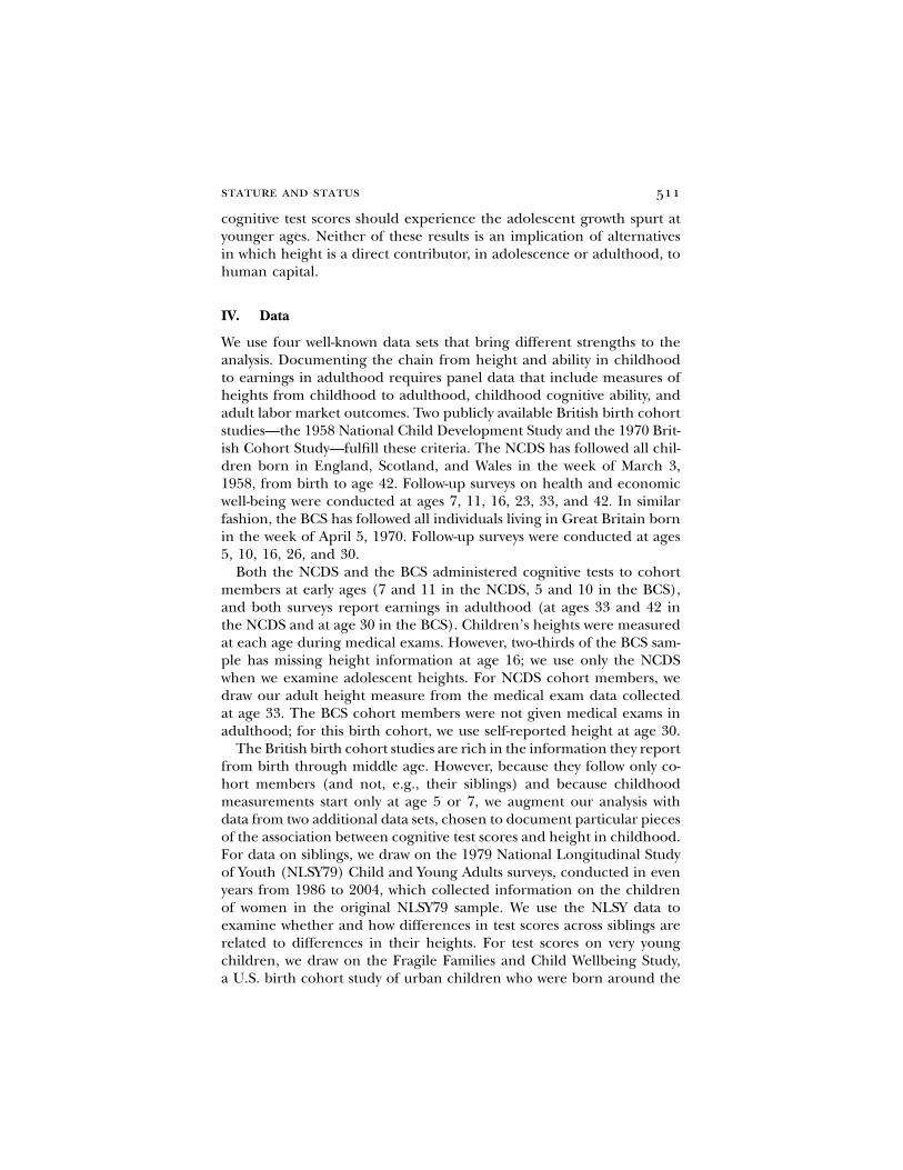
We use four well-known data sets that bring different strengths to theanalysis. Documenting the chain from height and ability in childhoodto earnings in adulthood requires panel data that include measures ofheights from childhood to adulthood, childhood cognitive ability, andadult labor market outcomes. Two publicly available British birth cohortstudies—the 1958 National Child Development Study and the 1970 Brit-ish Cohort Study—fulfill these criteria. The NCDS has followed all chil-dren born in England, Scotland, and Wales in the week of March 3,1958, from birth to age 42. Follow-up surveys on health and economicwell-being were conducted at ages 7, 11, 16, 23, 33, and 42. In similarfashion, the BCS has followed all individuals living in Great Britain bornin the week of April 5, 1970. Follow-up surveys were conducted at ages5, 10, 16, 26, and 30.

Both the NCDS and the BCS administered cognitive tests to cohortmembers at early ages (7 and 11 in the NCDS, 5 and 10 in the BCS),and both surveys report earnings in adulthood (at ages 33 and 42 inthe NCDS and at age 30 in the BCS). Children’s heights were measuredat each age during medical exams. However, two-thirds of the BCS sam-ple has missing height information at age 16; we use only the NCDSwhen we examine adolescent heights. For NCDS cohort members, wedraw our adult height measure from the medical exam data collectedat age 33. The BCS cohort members were not given medical exams inadulthood; for this birth cohort, we use self-reported height at age 30.

The British birth cohort studies are rich in the information they reportfrom birth through middle age. However, because they follow only co-hort members (and not, e.g., their siblings) and because childhoodmeasurements start only at age 5 or 7, we augment our analysis withdata from two additional data sets, chosen to document particular piecesof the association between cognitive test scores and height in childhood.For data on siblings, we draw on the 1979 National Longitudinal Studyof Youth (NLSY79) Child and Young Adults surveys, conducted in evenyears from 1986 to 2004, which collected information on the childrenof women in the original NLSY79 sample. We use the NLSY data toexamine whether and how differences in test scores across siblings arerelated to differences in their heights. For test scores on very youngchildren, we draw on the Fragile Families and Child Wellbeing Study,a U.S. birth cohort study of urban children who were born around the


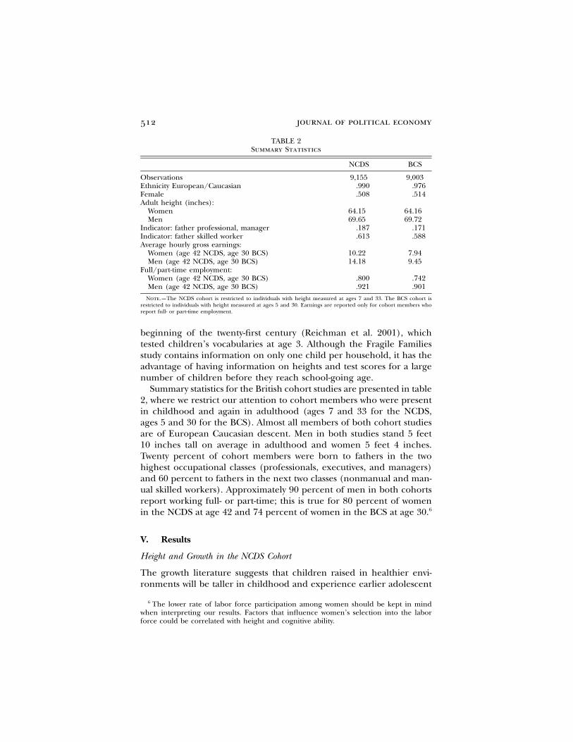
TABLE 2Summary Statistics

NCDS BCS

Observations 9,155 9,003Ethnicity European/Caucasian .990 .976Female .508 .514Adult height (inches):

Women 64.15 64.16Men 69.65 69.72

Indicator: father professional, manager .187 .171Indicator: father skilled worker .613 .588Average hourly gross earnings:

Women (age 42 NCDS, age 30 BCS) 10.22 7.94Men (age 42 NCDS, age 30 BCS) 14.18 9.45

Full/part-time employment:Women (age 42 NCDS, age 30 BCS) .800 .742Men (age 42 NCDS, age 30 BCS) .921 .901

Note.—The NCDS cohort is restricted to individuals with height measured at ages 7 and 33. The BCS cohort isrestricted to individuals with height measured at ages 5 and 30. Earnings are reported only for cohort members whoreport full- or part-time employment.

beginning of the twenty-first century (Reichman et al. 2001), whichtested children’s vocabularies at age 3. Although the Fragile Familiesstudy contains information on only one child per household, it has theadvantage of having information on heights and test scores for a largenumber of children before they reach school-going age.

Summary statistics for the British cohort studies are presented in table2, where we restrict our attention to cohort members who were presentin childhood and again in adulthood (ages 7 and 33 for the NCDS,ages 5 and 30 for the BCS). Almost all members of both cohort studiesare of European Caucasian descent. Men in both studies stand 5 feet10 inches tall on average in adulthood and women 5 feet 4 inches.Twenty percent of cohort members were born to fathers in the twohighest occupational classes (professionals, executives, and managers)and 60 percent to fathers in the next two classes (nonmanual and man-ual skilled workers). Approximately 90 percent of men in both cohortsreport working full- or part-time; this is true for 80 percent of womenin the NCDS at age 42 and 74 percent of women in the BCS at age 30.6

V. Results

Height and Growth in the NCDS Cohort

The growth literature suggests that children raised in healthier envi-ronments will be taller in childhood and experience earlier adolescent

6 The lower rate of labor force participation among women should be kept in mindwhen interpreting our results. Factors that influence women’s selection into the laborforce could be correlated with height and cognitive ability.


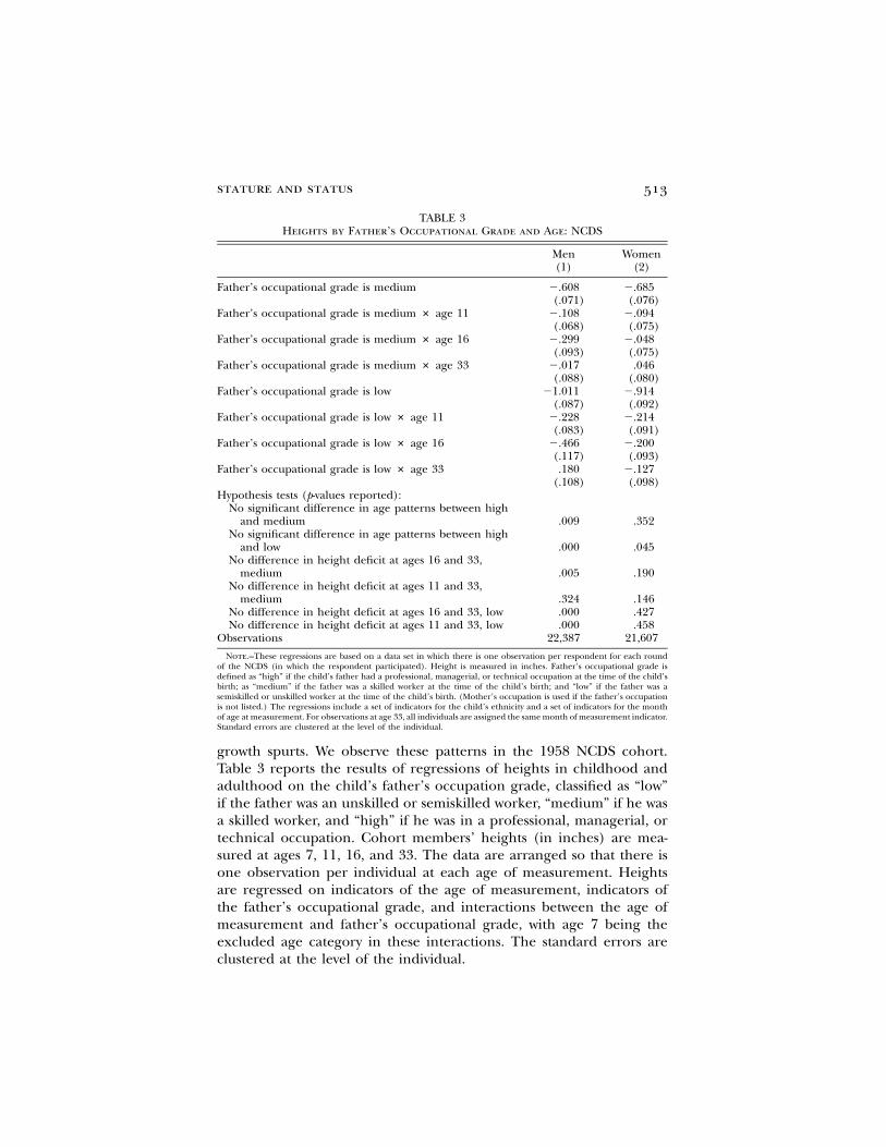
TABLE 3Heights by Father’s Occupational Grade and Age: NCDS

Men(1)

Women(2)

Father’s occupational grade is medium �.608(.071)

�.685(.076)

Father’s occupational grade is medium # age 11 �.108(.068)

�.094(.075)


�.048(.075)


.046(.080)

Father’s occupational grade is low �1.011(.087)

�.914(.092)

Father’s occupational grade is low # age 11 �.228(.083)

�.214(.091)

Father’s occupational grade is low # age 16 �.466(.117)

�.200(.093)

Father’s occupational grade is low # age 33 .180(.108)

�.127(.098)

Hypothesis tests (p-values reported):No significant difference in age patterns between high

and medium .009 .352No significant difference in age patterns between high

and low .000 .045No difference in height deficit at ages 16 and 33,

medium .005 .190No difference in height deficit at ages 11 and 33,

medium .324 .146No difference in height deficit at ages 16 and 33, low .000 .427No difference in height deficit at ages 11 and 33, low .000 .458

Observations 22,387 21,607

Note.–These regressions are based on a data set in which there is one observation per respondent for each roundof the NCDS (in which the respondent participated). Height is measured in inches. Father’s occupational grade isdefined as “high” if the child’s father had a professional, managerial, or technical occupation at the time of the child’sbirth; as “medium” if the father was a skilled worker at the time of the child’s birth; and “low” if the father was asemiskilled or unskilled worker at the time of the child’s birth. (Mother’s occupation is used if the father’s occupationis not listed.) The regressions include a set of indicators for the child’s ethnicity and a set of indicators for the monthof age at measurement. For observations at age 33, all individuals are assigned the same month of measurement indicator.Standard errors are clustered at the level of the individual.

growth spurts. We observe these patterns in the 1958 NCDS cohort.Table 3 reports the results of regressions of heights in childhood andadulthood on the child’s father’s occupation grade, classified as “low”if the father was an unskilled or semiskilled worker, “medium” if he wasa skilled worker, and “high” if he was in a professional, managerial, ortechnical occupation. Cohort members’ heights (in inches) are mea-sured at ages 7, 11, 16, and 33. The data are arranged so that there isone observation per individual at each age of measurement. Heightsare regressed on indicators of the age of measurement, indicators ofthe father’s occupational grade, and interactions between the age ofmeasurement and father’s occupational grade, with age 7 being theexcluded age category in these interactions. The standard errors areclustered at the level of the individual.


Consider, first, the results for men in column 1. They indicate that,at age 7, boys whose fathers were in the medium grade were 0.61 inchshorter on average than boys whose fathers were in the highest grade;boys whose fathers were in the lowest grade were 1.01 inches shorteron average than those whose fathers were in the highest grade. Thesedifferences in average heights across grades become larger as childrengrow older, taking their largest values at age 16. The average heightdeficit of boys with low-grade relative to high-grade fathers rises from1.01 inches at age 7, to 1.24 inches ( ) at age 11, and to�1.01 � 0.231.48 inches at age 16. This gap diminishes somewhat in adulthood, aslower-class boys experience some “catch-up” in height. Test statisticspresented at the bottom of the table show that, for boys whose fatherswere unskilled or semiskilled, height deficits at ages 11 and 16 aresignificantly larger than the height deficit at age 33.7

The gap in height between boys whose fathers were in the highestgrade and those in the medium grade is the same at age 33 as it wasat age 7; the interaction term for being in the medium group and beingage 33 is small and statistically insignificant, suggesting that those boysgrew more between 16 and 33 than boys in the high grade, in order toreturn to the gap they faced at age 7. The same is true for boys in thelow grade, who picked up 0.67 inch of height relative to high-gradeboys between age 16 (when they were an additional 0.47 inch shorterthan high-grade boys than they had been at age 7) and age 33 (whentheir height deficit has fallen to below the level it had been at age 7 by0.18 inch).

The results for women are somewhat different. At age 7, girls whosefathers were in professional occupations are 0.7 inch taller on averagethan girls whose fathers were skilled workers and 0.9 inch taller thangirls whose fathers were semi- or unskilled workers. The point estimatesindicate that the differences in average heights between women withlow-grade and medium-grade fathers, relative to those with high-gradefathers, reach their largest values at age 11 (�0.914 � 0.214 p�1.128 for girls in the lowest category at age 11). However, the deficitsat ages 11 and 16 are similar to each other and are not significantlydifferent from their values at age 33. The difference in results betweenmen and women may be due to the earlier adolescent growth spurtexperienced by girls and the timing of the NCDS surveys. Girls’ peakheight velocity occurs, on average, closer to the age 11 survey than tothe age 16 survey. Nearly all girls will have completed their adolescentgrowth spurts by age 16, which is not true for boys. While we find

7 That children in the NCDS from poorer backgrounds have “a delayed pattern of growthbefore the pubertal spurt, followed by catch-up growth” has been noted earlier by Li,Manor, and Power (2004, 185).


significant differences in the growth patterns of girls from higher-statusand lower-status backgrounds, in the absence of information on heightsat each age in adolescence, it is not possible to tell whether the differ-ences in average heights between girls from more and less advantagedbackgrounds become more pronounced during the period of peakheight velocity.

These results have several implications for the analysis of the rela-tionship between earnings and heights at different ages. First, they in-dicate that heights in both childhood and adulthood are associated withthe economic status of a child’s family. As discussed above, this associ-ation may reflect a combination of genetic and environmental factorsthat also drive productivity in the labor market. A second implicationis that growth patterns throughout childhood may convey more infor-mation about endowments than heights in adulthood alone. For boys,especially, height at age 16 may be a good marker for unobserved ability.We return to this below when we examine the relationship betweenearnings and heights at different ages in childhood.

Height and Childhood Cognitive Test Scores

We present direct evidence on the relationship between height and testscores in childhood in table 4, using data from the NCDS and the BCS.The tests administered to children vary across ages and surveys. For the5-year-olds in the BCS, we show results for a human figure drawingscore, which provides a measure of conceptual maturity; a copy designtest that measures visual-motor coordination; and the English PictureVocabulary Test (EPVT) score, which measures the size of the child’svocabulary. At age 10, we show results for the four subscales of the BritishAbility Scales (BAS) included in the BCS. We chose to report theserather than scores on the math, reading, and vocabulary tests that weregiven at age 10, since the BAS subscales are meant to measure cognitiveability rather than academic achievement.8 For the NCDS, we show re-sults for the human figure drawing test and math and reading scores

8 That said, regression results for standardized vocabulary and math tests are very similarto those for the BAS test scores at age 10. Each inch of height is associated with approx-imately a 10 percent of a standard deviation increase in the Pictorial Language Compre-hension Test and in the Friendly Maths Test in the absence of extended controls. Thecoefficient on the height for age 5 z-score for the verbal test is 0.111 (standard error0.009) and for the math test is 0.121 (0.010). Similarly to the BAS results, with extendedcontrols, these coefficients fall by half, to 0.046 (0.010) for the vocabulary test and to0.054 (0.010) for the math test. Results for the Edinburgh Reading Test are less pro-nounced, with a coefficient on height taking a value of 0.047 (0.010) in the absence ofextended controls and 0.008 (0.011) in their presence. These results do not support amodel in which taller children are spurred on by teachers or the social setting of theclassroom to outperform shorter peers. If they were, we would expect larger height effectsfor tests of academic achievement than for cognitive ability.

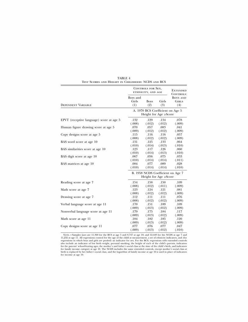
TABLE 4Test Scores and Height in Childhood: NCDS and BCS

Dependent Variable

Controls for Sex,ethnicity, and age Extended

Controls:Boys and

Girls(4)

Boys andGirls(1)

Boys(2)

Girls(3)

A. 1970 BCS Coefficient on Age 5Height for Age z-Score

EPVT (receptive language) score at age 5 .132(.008)

.129(.012)

.134(.012)

.078(.009)

Human figure drawing score at age 5 .070(.009)

.057(.012)

.083(.012)

.041(.009)

Copy designs score at age 5 .115(.008)

.116(.012)

.116(.012)

.057(.009)

BAS word score at age 10 .131(.010)

.125(.014)

.133(.013)

.064(.010)

BAS similarities score at age 10 .123(.010)

.117(.014)

.126(.013)

.060(.010)

BAS digit score at age 10 .067(.010)

.056(.014)

.075(.014)

.033(.011)

BAS matrices at age 10 .084(.010)

.077(.014)

.089(.014)

.028(.010)

B. 1958 NCDS Coefficient on Age 7Height for Age z-Score

Reading score at age 7 .154(.008)

.158(.012)

.150(.011)

.109(.009)

Math score at age 7 .123(.008)

.124(.012)

.121(.012)

.081(.009)

Drawing score at age 7 .112(.008)

.111(.012)

.111(.012)

.076(.009)

Verbal language score at age 11 .170(.009)

.151(.013)

.189(.012)

.109(.009)

Nonverbal language score at age 11 .179(.009)

.175(.013)

.184(.012)

.117(.009)

Math score at age 11 .184(.009)

.182(.013)

.185(.012)

.120(.009)

Copy designs score at age 11 .077(.009)

.076(.013)

.077(.012)

.047(.010)

Note.—Samples sizes are 11,360 for the BCS at age 5 and 8,747 at age 10; and 12,449 for the NCDS at age 7 and11,232 at age 11. All regressions control for the age of the child at measurement, a set of ethnicity indicators, and (forregressions in which boys and girls are pooled) an indicator for sex. For the BCS, regressions with extended controlsalso include an indicator of low birth weight, prenatal smoking, the height of each of the child’s parents, indicatorsfor the parents’ school-leaving ages, the mother’s and father’s social class at the time of the child’s birth, and indicatorsfor family income category at age 10. The NCDS includes the same extended controls, except mother’s social class atbirth is replaced by her father’s social class, and the logarithm of family income at age 16 is used in place of indicatorsfor income at age 10.


at age 7, and scores from verbal language, nonverbal language, math,and copy design tests at age 11. All tests are standardized within thesample to have a mean of zero and a standard deviation of one, andthe height measures are transformed into height for age z-scores usingthe 2000 growth charts from the Centers for Disease Control (2002).This standardization makes it easier to compare estimates across agesand tests.

For both surveys, we first show results of regressions of test scores onheight, controlling for only a few key variables: the child’s sex, ethnicity,and the age in months at which the testing occurred. We then showresults (in col. 4) that include an extended set of family backgroundvariables including the family’s economic status, parent’ education levelsand their heights, prenatal smoking, and an indicator that the child wasborn at low weight. These controls, which are listed in the note to table4, are associated with heights in childhood and adulthood.9 We expectthat the covariance between height and cognitive test scores will besmaller after conditioning on these variables, since better-off childrenboth are taller and have higher test scores. However, approximately two-thirds to three-quarters of the cross-sectional variation in heights is notexplained by these variables, and it is of interest to know if the corre-lation between height and cognitive ability persists even after observabledeterminants of height are accounted for.10

We find a large and significant association between height and testscores for children followed in the BCS for tests they took at ages 5 and10 (panel A) and for children in the NCDS for tests at ages 7 and 11(panel B). The coefficients are somewhat larger for the NCDS, especiallyamong 11-year-olds, but the patterns across the two cohort studies arequite similar. In neither study does it appear that the associations are

9 Heights are correlated with observable factors that are likely to be determinants ofcognitive development. In an earlier version of this paper, we presented results of re-gressions, from the NCDS, of boys’ heights at different ages on measures of the child’sfamily’s socioeconomic status, including parental education and occupational-based mea-sures of social class; measures of the child’s health at birth, including low birth weightand prenatal smoking; and measures of parents’ heights. All three sets of factors aresignificant predictors of height. Together, these variables explain between 25 and 33percent of the variation in heights, with parental heights—which may reflect genetic factorsor parents’ childhood circumstances—providing the largest incremental contribution tothe .2R

10 If height is capturing unobservable components of endowments, then the coefficienton height should go to zero as all unobservables are accounted for. Murphy and Topel(1990) suggest that the impact of remaining unobservables on a coefficient can be assessedby extrapolation, which, in this case, means computing the change in the coefficient onheight relative to the change in the that occurs when the family background measures2Rare included and calculating what the coefficient on height would be if the were equal2Rto one. However, when we do this, the extrapolated coefficient on height is large andnegative. The key assumption necessary for the Murphy and Topel result to hold (thatthe remaining unobservables are correlated with height to the same degree as the extraobservables that have been added to the regression) may be unlikely to hold in our case.


TABLE 5Test Scores and Height in Childhood: Children of the NLSY and Fragile

Families

Dependent Variable

LimitedControls

(1)

ExtendedControls

(2)

ExtendedControls

(3)Observations

(4)

A. Children of the NLSY, Coefficient on Age 5–6Height for Age z-Score

PIAT mathematics .067(.007)

.052(.007)

.031(.010)

13,834

PIAT reading recognition .059(.007)

.044(.007)

.028(.010)

13,702

PIAT reading comprehension .061(.008)

.051(.008)

.025(.012)

9,605

PPVT .068(.011)

.050(.011)

0.027(.016)

5,227

Digit span .056(.010)

.048(.011)

.018(.016)

7,042

B. Fragile Families Coefficient on Age 3 Height forAge z-Score

PPVT .089(.020)

.052(.020)

2,150

Mother fixed effects? No No Yes

Note.—Panel A shows coefficients and standard errors from OLS regressions on the Children of the NLSY, whosecognitive function was evaluated multiple times between ages 5 and 10. Each coefficient comes from a separate regression,where the reported coefficients are those on the age 5–6 height for age z-score. All regressions include controls forage at the time of the assessment at ages 5–6; a quartic in age at the time of each assessment; and indicators for race,sex, and year. Extended controls include an indicator for low birth weight and indicators for the number of packs ofcigarettes the mother smoked during pregnancy, mother’s height in 1985, mother’s AFQT score in 1989, total householdincome in the previous calendar year, indicators for the highest grade completed by the mother, and indicators thatthe mother’s partner lives in the household and indicators that the child’s maternal grandmother and grandfather livein the household. For the Fragile Families results, all regressions include indicators for gender and age in months atthe time of measurement. The extended controls include an indicator for low birth weight, the heights of both parents,indicators for the educational attainment of both parents, indicators for the maternal grandfather’s education, thelogarithm of family income at age 3, the mother’s score on the PPVT, and an indicator of whether the mother tookthe Spanish-language version of the PPVT (i.e., the Test de Vocabulario en Imagenes Peabody).

systematically larger for older versus younger children. The magnitudesof these associations are quite large, even when the extended controlsare included. For example, in the NCDS data using extended controls,a one standard deviation increase in height at age 7 is associated witha 10 percent of a standard deviation increase in reading score at age 7and in verbal language score at age 11. This effect is as large as thatpredicted by a two standard deviation increase in log household incomefor these children.11

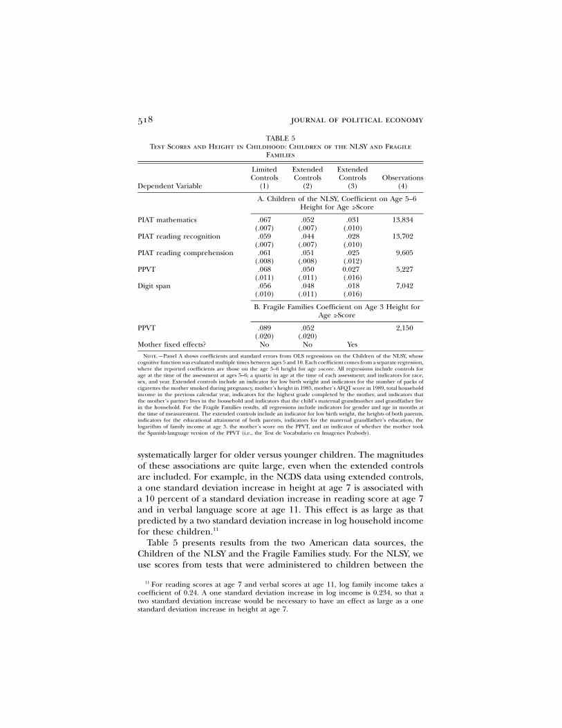
Table 5 presents results from the two American data sources, theChildren of the NLSY and the Fragile Families study. For the NLSY, weuse scores from tests that were administered to children between the

11 For reading scores at age 7 and verbal scores at age 11, log family income takes acoefficient of 0.24. A one standard deviation increase in log income is 0.234, so that atwo standard deviation increase would be necessary to have an effect as large as a onestandard deviation increase in height at age 7.


ages of 5 and 10. The tests include the Peabody Individual AchievementTests (PIAT) for mathematics, reading recognition, and reading com-prehension, a digit span test, and the Peabody Picture Vocabulary Test(PPVT). The digit span test measures a child’s short-term memory. ThePPVT, on which the EPVT is based, is a test of receptive vocabulary thatcan be administered to individuals from age 30 months through adult-hood, and it has been used in numerous studies of preschool and school-aged children (Dunn and Dunn 1997). The PPVT was also administeredto the 3-year-olds from the Fragile Families study.

For both samples, we use a set of extended controls that is comparableto those used in our analyses of the British data. One difference, how-ever, is that both the NLSY and the Fragile Families samples containinformation on the cognitive ability of mothers, in the form of an ArmedForces Qualifying Test (AFQT) score for the mothers in the NLSY andthe PPVT for the mothers in the Fragile Families data. The NLSY hasthe additional advantage of containing information on all of themother’s children, making it possible to control for mother-specificfixed effects.

The results from the NLSY indicate that children’s heights are stronglyassociated with test scores. The point estimates are somewhat smallerthan in the British data. For example, the coefficient for height for thePPVT is 0.069, in contrast to the coefficient of 0.132 for the EPVT takenby 5-year-olds in the BCS. The addition of extended controls reducesthe height coefficients to approximately 75 percent of their originalvalues; adding mother fixed effects reduces coefficients to approxi-mately half of their original values. However, with the exception of thedigit span test, a child’s height remains a significant correlate of his orher test scores, even in the presence of mother fixed effects. The heightcoefficients in column 3 are identified entirely off of between-siblingdifferences in height for age z-scores at age 5 and differences in theirtest scores. It is not possible to attribute either the attenuation of thecoefficients in the presence of mother effects or their continued sig-nificance to a child’s environment, genes, or gene-environment inter-actions. Siblings could differ in their heights and their test scores be-cause the household environment one was born into could have beenhealthier and more stable in a manner not captured by our extendedcontrols. Differences in heights could also be due to differences in thegenetic material obtained from parents, or the interaction of the two.Without more information, it is not possible to say more than this.However, we can say that, even when we control for the genetic materialsiblings share and for that part of their home environment that is con-stant, children who were taller at ages 5 and 6 outperform shortersiblings on cognitive tests throughout childhood.

One possible explanation for the results discussed above is that taller


children may be provided with greater levels of cognitive stimulation atschool, possibly even as early as kindergarten. Teachers may pay moreattention to taller children, or taller children may be more likely to beenrolled in school earlier than shorter children of the same age. How-ever, evidence from the 3-year-old children from the Fragile Familiesstudy indicates that the association between height and cognitive abilityappears before children reach school-going age. A one standard devi-ation increase in height is associated with a 5–10 percent of a standarddeviation increase in the PPVT score at age 3. Estimates of separateregressions for boy and girls (not shown) yield similar results. Includingextended controls (which, in this case, include the mother’s own PPVTscore) reduces but does not eliminate the association between heightsand test scores. These results indicate that the correlation betweenheight and cognitive ability is present before any potential differentialtreatment of taller children in school.12 That the associations betweenheight and test scores do not systematically rise with age suggests thatthese associations are not magnified by the behaviors of teachers orparents later in life.

We also use data on the Children of the NLSY to examine the extentto which height differences explain differences in test scores across racialand ethnic groups in the United States. Estimating separate height co-efficients for Hispanic, African American, and white non-Hispanic chil-dren in regressions that also contain a quartic in age at testing, indicatorsfor race (African American) and ethnicity (Hispanic), and indicatorsfor the year the test was taken, we find no significant differences inheight premia between white, African American, and Hispanic children.For all groups, the height premium is significant for PIAT mathematics,reading recognition, reading comprehension, and digit span tests, withcoefficients on height for age z-scores at age 5 on the order of 0.05–0.08 for all three groups. Hispanic and African American Children ofthe NLSY on average have lower scores for all these tests in the absenceof height measures. Inclusion of height for age z-scores does nothingto the coefficients on race and ethnicity. Not only are they not signifi-cantly different with and without controls for height, the point estimatesare also almost identical. Within a group, height provides a marker forcognitive function, but height does not explain differences in scoresbetween groups.

Other evidence indicates that the association between height andcognitive ability persists through life. Abbott et al. (1998) document asignificant correlation between height of men in midlife and their cog-

12 There is only limited evidence on the association between height and cognitive abilityat ages younger than 3. However, one study of Indian children found that the length of5–12-month-old infants is associated with measures of information processing speed (Rose1994).


nitive performance after age 70. Even after adjustment for educationand father’s occupation, they find a strong and significant associationbetween height and cognitive function in old age. Case and Paxson(2008) similarly document a strong positive association between heightand cognition among older men and women followed in the U.S. Healthand Retirement Study.

Height, Cognitive Ability, and Earnings

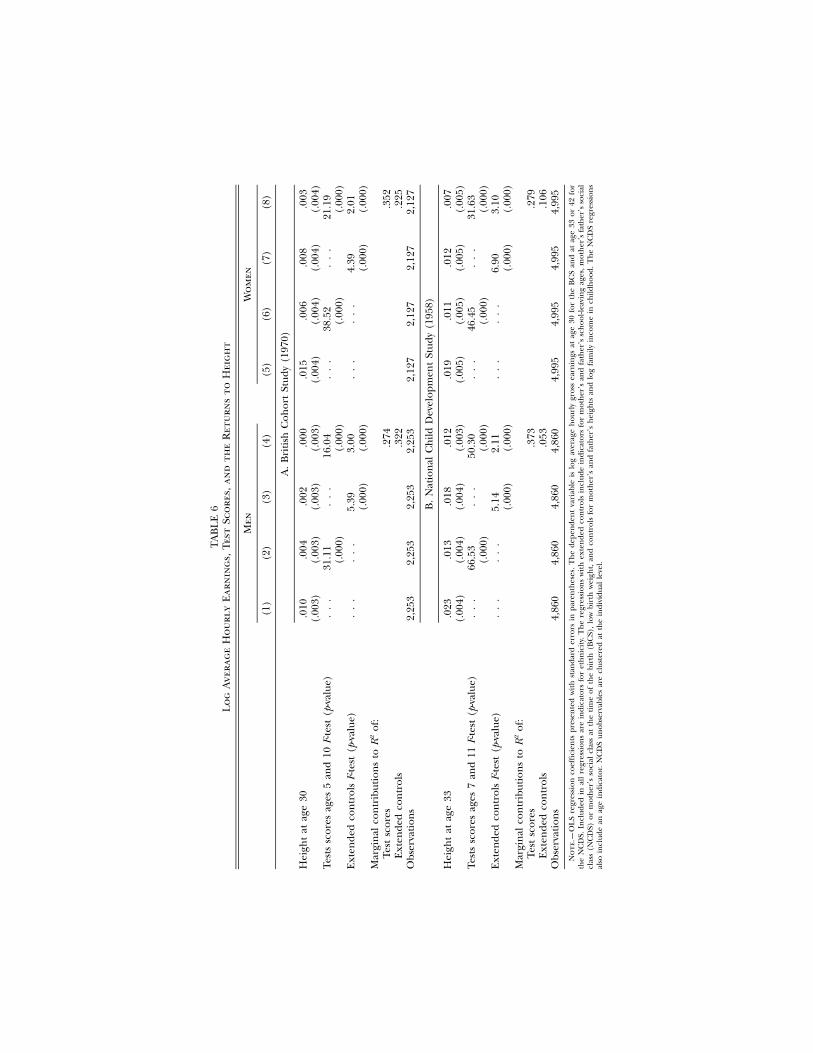
We use data from the British birth cohorts to reexamine the heightpremia in earnings presented in table 1, drawing on the informationwe have on cognitive ability and family background. Table 6 presentsthe results of regressions of the logarithm of average hourly earningson adult height. Panel A shows results for men and women in the 1970BCS and panel B for the 1958 NCDS. We restrict our sample to indi-viduals who took cognitive tests at two points in childhood: ages 5 and10 for the BCS cohort and ages 7 and 11 for the NCDS. The BCS samplecontains one observation per individual: both height and average hourlyearnings are reported by the individual at age 30. The NCDS samplecontains up to two observations on average hourly earnings per indi-vidual: one from the age 33 survey and another from the age 42 survey.For the NCDS, we use the value of height from the age 33 survey, whichwas measured during a medical examination. Columns 1 and 4 of table6 repeat the coefficients shown for the log of average hourly earningsin table 1.

Looking first at the results for the BCS cohort, in panel A, we findthat test scores are jointly highly significant in the BCS earnings equa-tions, with F-tests of 31.1 for men and 38.5 for women. Inclusion ofthese cognitive test scores reduces the size of the height coefficients bymore than 50 percent and renders them statistically insignificant. Bothtest scores and height are correlated with family background, and it isinteresting to see the extent to which family background can explainthe height premia. The inclusion of personal and parental backgroundcharacteristics, with no controls for test scores, also reduces the heightpremia in earnings in the BCS cohort, more so for men than for women.This reduction in the height premia, in the presence of extended con-trols, is not surprising: if height is a marker for cognitive ability, thenincluding determinants of cognitive ability (parents’ education and co-hort members’ early-life health, e.g.) should weaken the associationbetween height and earnings. When both test scores and backgroundcharacteristics are controlled for (cols. 4 and 8), we again find no evi-dence of a height premium in earnings. Both the test scores and back-ground measures are jointly significant, although the F-statistics for thetest scores are substantially larger than those for the extended back-

TA

BL

E6

Lo

gA

vera

ge

Ho

url

yE

arn

ing

s,Te

stSc

ore

s,an

dth

eR

etu

rns

toH

eig

ht

Men

Wo

men

(1)

(2)

(3)

(4)

(5)

(6)

(7)

(8)

A.

Bri

tish

Coh

ort

Stud

y(1

970)

Hei

ght

atag

e30

.010

(.00

3).0

04(.

003)

.002

(.00

3).0

00(.

003)

.015

(.00

4).0

06(.

004)

.008

(.00

4).0

03(.

004)

Test

ssc

ores

ages

5an

d10

F-te

st(p

-val

ue)

..

.31

.11

(.00

0).

..

16.0

4(.

000)

..

.38

.52

(.00

0).

..

21.1

9(.

000)

Ext

ende

dco

ntr

ols

F-te

st(p

-val

ue)

..

..

..

5.39

(.00

0)3.

00(.

000)

..

..

..

4.39

(.00

0)2.

01(.

000)

Mar

gin

alco

ntr

ibut

ion

sto

of:

2R

Test

scor

es.2

74.3

52E

xten

ded

con

trol

s.3

22.2

25O

bser

vati

ons

2,25

32,

253

2,25

32,

253

2,12

72,

127

2,12

72,

127

B.

Nat

ion

alC

hild

Dev

elop

men

tSt

udy

(195

8)

Hei

ght

atag

e33

.023

(.00

4).0

13(.

004)

.018

(.00

4).0

12(.

003)

.019

(.00

5).0

11(.

005)

.012

(.00

5).0

07(.

005)

Test

ssc

ores

ages

7an

d11

F-te

st(p

-val

ue)

..

.66

.53

(.00

0).

..

50.3

0(.

000)

..

.46

.45

(.00

0).

..

31.6

3(.

000)

Ext

ende

dco

ntr

ols

F-te

st(p

-val

ue)

..

..

..

5.14

(.00

0)2.

11(.

000)

..

..

..

6.90

(.00

0)3.

10(.

000)

Mar

gin

alco

ntr

ibut

ion

sto

of:

2R

Test

scor

es.3

73.2

79E

xten

ded

con

trol

s.0

53.1

06O

bser

vati

ons

4,86

04,

860

4,86

04,

860

4,99

54,

995

4,99

54,

995

No

te.—

OL

Sre

gres

sion

coef

fici

ents

pres

ente

dw

ith

stan

dard

erro

rsin

pare

nth

eses

.T

he

depe

nde

nt

vari

able

islo

gav

erag

eh

ourl

ygr

oss

earn

ings

atag

e30

for

the

BC

San

dat

age

33or

42fo

rth

eN

CD

S.In

clud

edin

all

regr

essi

ons

are

indi

cato

rsfo

ret

hn

icit

y.T

he

regr

essi

ons

wit

hex

ten

ded

con

trol

sin

clud

ein

dica

tors

for

mot

her

’san

dfa

ther

’ssc

hoo

l-lea

vin

gag

es,m

oth

er’s

fath

er’s

soci

alcl

ass

(NC

DS)

orm

oth

er’s

soci

alcl

ass

atth

eti

me

ofth

ebi

rth

(BC

S),

low

birt

hw

eigh

t,an

dco

ntr

ols

for

mot

her

’san

dfa

ther

’sh

eigh

tsan

dlo

gfa

mily

inco

me

inch

ildh

ood.

Th

eN

CD

Sre

gres

sion

sal

soin

clud

ean

age

indi

cato

r.N

CD

Sun

obse

rvab

les

are

clus

tere

dat

the

indi

vidu

alle

vel.


ground controls. For the BCS, the marginal contribution of the testscores to the of the regressions is similar in magnitude to the marginal2Rcontribution for the extended controls.

Panel B repeats this analysis for the NCDS. In general, the coefficientson height are larger than they were using the BCS, possibly because,with measured rather than self-reported adult heights, there may be lessattenuation bias due to measurement error.13 Even after the inclusionof controls for test scores, background characteristics, and the combi-nation of the two, the height premium in average hourly earnings formen (but not for women) is still statistically significant. However, theinclusion of test scores and extended controls reduces the height pre-mium in average hourly earnings by 48 percent for men and 63 percentfor women. The NCDS results differ from the BCS results in that themarginal contribution of test scores to the of the earnings equation2Ris substantially larger for both men and women (0.373, 0.279) than themarginal contribution of the extended controls (0.053, 0.106).14

On average, women earn less than men in both birth cohorts. How-ever, the height difference between men and women does not explainwomen’s lower earnings. When we combine the samples of men andwomen and estimate a regression of log hourly earnings on an indicatorthat the cohort member is male, controlling for height, cognitive ability,and family background, the wage premium for men in the 1958 birthcohort is 40 percent, with or without controlling for height in the re-gression. In the 1970 birth cohort, the male wage premium is lower, at17 percent, with or without the inclusion of height.

Growth, Cognitive Ability, and Earnings

The framework developed above suggests that patterns of growth duringchildhood contain information about children’s endowments. One im-plication of the model is that if both cognitive ability and growth aredriven by the same underlying endowment, then cognitive ability inchildhood should be correlated with the timing of the adolescent growth

13 Because members of the NCDS were measured at age 33 and self-reported their heightsat age 42, we can examine the extent to which self-reports would lead to attenuation biasin this sample. Repeating regressions reported in table 1 for log hourly earnings in theNCDS, but using self-reported heights in place of measured heights, we find that thecoefficient for men’s heights falls from 0.023 to 0.018. The coefficient on women’s heightsremains unchanged at 0.019. (Women in the NCDS are 10 percentage points less likelythan men to report themselves as taller at age 42 than they were measured to be at age33.)

14 The key difference in this result between the cohort studies is that father’s school-leaving age is a much stronger predictor of earnings among members of the 1970 cohortthan among members of the 1958 cohort.


spurt. Specifically, children who have higher cognitive test scores shouldexperience their adolescent growth spurts at younger ages.

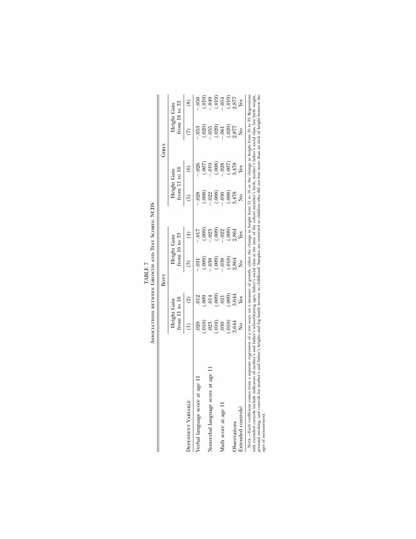
We use data from the NCDS to examine whether cognitive test scoresat age 11 are associated with the timing of the adolescent growth spurt.We first regress individual test scores on growth between ages 11 and16 and then on growth between ages 16 and 33. We estimate separatemodels for boys and girls. Because girls begin their adolescent growthspurts earlier than boys, the associations between growth at differentages and cognitive ability should vary by sex. We also estimate thesemodels with and without a set of extended controls for family charac-teristics that measure parents’ height and educational attainment, eco-nomic status, and measures of a cohort member’s health in early life,specifically whether the child was born at low weight and whether hisor her mother smoked during pregnancy. We expect these extendedcontrols to be associated with both test scores and the timing of theadolescent growth spurt.

Columns 1–4 of table 7 present evidence that the timing of growthis a marker of cognitive function in boys. Boys who grew more fromage 11 to 16 had, on average, higher cognitive test scores at age 11.The results in column 1 indicate that each inch of growth in earlyadolescence is associated with an increase in test scores at age 11 ofbetween 2 and 3 percent of a standard deviation. In contrast, boys whogrew more between ages 16 and 33—indicating a later adolescent growthspurt—had lower average test scores at age 11. Each inch of growth inlate adolescence is associated with a decline in test scores at age 11 ofbetween 3.1 and 3.8 percent of a standard deviation. As expected, thesizes of these associations for both growth periods are smaller in absolutevalue when extended controls that may be determinants of both thetempo of growth and cognitive function are included.

The results for girls differ from those for boys, in ways that makesense given girls’ earlier adolescent growth spurts. Height gains from11 to 16 are negatively associated with test scores at age 11, with eachinch of height associated with a decline in test scores ranging from 2.2to 3.0 percent of a standard deviation. Height gains from 16 to 33 haveeven larger negative associations with test scores, with coefficients of�5.3 to �6.1. The girls with the highest test scores at age 11 had alreadyattained a large share of their adult heights, so that growth from 11 to16 signals relatively “late” growth.15 By age 16, most girls have attained

15 Ideally, we would have height measurements for girls at the age of 8 or 9, just beforethe adolescent growth spurt, and at age 12 or 13, just after the average age of peak heightvelocity for girls. We expect that test scores would be positively associated with growthfrom age 8 to 12 and negatively associated with growth from age 12 to 16. We are, however,unable to test this with the NCDS.

TA

BL

E7

Ass

oci

atio

ns

betw

een

Gro

wth

and

Test

Sco

res:

NC

DS

Bo

ysG

irls

Hei

ght

Gai

nfr

om11

to16

Hei

ght

Gai

nfr

om16

to33

Hei

ght

Gai

nfr

om11

to16

Hei

ght

Gai

nfr

om16

to33

Dep

end

ent

Vari

able

(1)

(2)

(3)

(4)

(5)

(6)

(7)

(8)

Verb

alla

ngu

age

scor

eat

age

11.0

20(.

010)

.012

(.00

9�

.031

(.00

9)�

.017

(.00

9)�

.028

(.00

8)�

.026

(.00

7)�

.053

(.02

0)�

.050

(.01

9)N

onve

rbal

lan

guag

esc

ore

atag

e11

.023

(.01

0).0

14(.

009)

�.0

38(.

009)

�.0

23(.

009)

�.0

22(.

008)

�.0

19(.

008)

�.0

55(.

020)

�.0

49(.

019)

Mat

hsc

ore

atag

e11

.030

(.01

0).0

21(.

009)

�.0

38(.

010)

�.0

22(.

009)

�.0

30(.

008)

�.0

28(.

007)

�.0

61(.

020)

�.0

54(.

019)

Obs

erva

tion

s3,

644

3,64

42,

864

2,86

43,

478

3,47

82,

877

2,87

7E

xten

ded

con

trol

s?N

oYe

sN

oYe

sN

oYe

sN

oYe

s

No

te.—

Eac

hco

effi

cien

tco

mes

from

ase

para

tere

gres

sion

ofa

test

scor

eon

am

easu

reof

grow

th,

eith

erth

ech

ange

inh

eigh

tfr

om11

to16

orth

ech

ange

inh

eigh

tfr

om16

to33

.R

egre

ssio

ns

wit

hex

ten

ded

con

trol

sin

clud

ein

dica

tors

ofm

oth

er’s

and

fath

er’s

sch

ool-l

eavi

ng

ages

,fa

ther

’sso

cial

clas

sat

the

tim

eof

the

coh

ort

mem

ber’

sbi

rth

,m

oth

er’s

fath

er’s

soci

alcl

ass,

low

birt

hw

eigh

t,pr

enat

alsm

okin

g,an

dco

ntr

ols

for

mot

her

’san

dfa

ther

’sh

eigh

tsan

dlo

gfa

mily

inco

me

inch

ildh

ood.

Sam

ples

are

rest

rict

edto

child

ren

wh

odi

dn

otlo

sem

ore

than

anin

chof

hei

ght

betw

een

the

ages

ofm

easu

rem

ent.


their adult height. Growth from age 16 to 33 is a signal of more severedeprivation than is the case for boys.

The results in table 7 indicate that, for both boys and girls, the patternsof heights over childhood convey information about children’s cognitiveability. If so, then heights at different periods in childhood, even whenwe control for adult height, should be associated with earnings in adult-hood. Our reading of the literature from human biology indicates thatheight during the adolescent growth spurt is likely to be an especiallygood marker of a child’s endowment. Heights in young childhood mayalso convey more information about early-life experiences than heightin middle childhood or adulthood. Furthermore, if the associationsbetween heights and earnings reflect cognitive ability, then the inclusionof measures of cognitive ability in earnings regressions should reducethe associations between heights and earnings.

To examine these hypotheses, in table 8 we use the NCDS to estimateregressions of the logarithm of average hourly earnings of men andwomen on their heights at ages 7, 11, 16, and 33, with and withoutcontrols for test scores and other extended controls. Our results formen in column 1 indicate that heights at ages 7 and 16 are significantlyassociated with average hourly earnings, with coefficients of 0.022 and0.017, respectively. The coefficients for heights at ages 11 and 33 aremuch smaller (both 0.001) and insignificant, and the hypothesis thatthe four height coefficients are equal can be strongly rejected. Theinclusion of test scores at ages 7 and 11 produces reductions in thecoefficients for heights at ages 7 and 11: the coefficient on height atage 7 is not significant, and that for height at age 16 is reduced by 24percent. The inclusion of extended controls alone has much smallereffects, and the coefficients with both test scores and extended controlsare much the same as with test scores alone. These results are consistentwith those in table 6, which showed that, with height at age 33, theheight premium in earnings for men is reduced but not eliminatedwhen we control for childhood test scores.

These reductions in the height premia in earnings are much morepronounced if we also control for test scores at age 16. For example, avariant of column 2 of table 8 that includes age 16 test scores yields acoefficient on height at age 16 of 0.007, with a standard error of 0.006.We have chosen not to control for age 16 test scores, since it is possiblethat taller adolescent boys, because of their heights, have more positiveadolescent experiences, which could result in higher test scores at age16 (Persico et al. 2004). We discuss this hypothesis in more detail below.

The associations between heights at different points in childhood andearnings are less informative for women than for men. Heights at ages7 and 33 take the largest coefficients, although neither is precisely es-timated, and the hypothesis that the coefficients on heights are identical

TA

BL

E8

Lo

gA

vera

ge

Ho

url

yE

arn

ing

s,Te

stSc

ore

s,an

dth

eR

etu

rns

toH

eig

ht:

1958

NC

DS

Men

Wo

men

(1)

(2)

(3)

(4)

(5)

(6)

(7)

(8)

Hei

ght

atag

e7

.022

(.00

7).0

07(.

007)

.018

(.00

7).0

06(.

007)

.011

(.00

8).0

01(.

008)

.006

(.00

8)�

.001

(.00

8)H

eigh

tat

age

11�

.001

(.00

7)�

.001

(.00

6)�

.003

(.00

7)�

.003

(.00

6).0

06(.

006)

.002

(.00

5).0

05(.

006)

.002

(.00

5)H

eigh

tat

age

16.0

17(.

005)

.013

(.00

5).0

16(.

005)

.013

(.00

5)�

.004

(.00

8)�

.005

(.00

8)�

.008

(.00

8)�

.007

(.00

8)H

eigh

tat

age

33.0

01(.

005)

.002

(.00

4).0

01(.

005)

.002

(.00

4).0

11(.

007)

.011

(.00

7).0

09(.

007)

.010

(.00

7)F-

test

:h

eigh

tva

riab

les

(p-v

alue

)18

.24

(.00

0)6.

04(.

000)

12.3

2(.

000)

5.11

(.00

0)6.

34(.

000)

1.49

(.20

4)2.

39(.

049)

.73

(.56

9)Te

sts

scor

esag

es7

and

11F-

test

(p-v

alue

)61

.83

(.00

0)48

.00

(.00

0)46

.78

(.00

0)32

.11

(.00

0)E

xten

ded

con

trol

sF-

test

(p-v

alue

)4.

91(.

000)

2.06

(.00

0)6.

72(.

000)

3.06

(.00

0)O

bser

vati

ons

4,86

04,

860

4,86

04,

860

4,99

54,

995

4,99

54,

995

No

te.—

OL

Sre

gres

sion

coef

fici

ents

pres

ente

dw

ith

stan

dard

erro

rsin

pare

nth

eses

.T

he

depe

nde

nt

vari

able

islo

gav

erag

eh

ourl

ygr

oss

earn

ings

atag

e33

or42

.T

he

stan

dard

erro

rsar

ecl

uste

red

atth

ele

vel

ofth

ein

divi

dual

.In

clud

edin

all

regr

essi

ons

are

indi

cato

rsfo

ret

hn

icit

yan

dan

indi

cato

rfo

rw

het

her

the

indi

vidu

alw

as33

or42

atth

eda

teea

rnin

gsw

ere

mea

sure

d.T

he

regr

essi

onw

ith

exte

nde

dco

ntr

ols

incl

udes

indi

cato

rsof

mot

her

’san

dfa

ther

’ssc

hoo

l-lea

vin

gag

es,m

oth

er’s

fath

er’s

soci

alcl

ass,

low

birt

hw

eigh

t,an

dco

ntr

ols

for

mot

her

’san

dfa

ther

’sh

eigh

tsan

dlo

gfa

mily

inco

me

inch

ildh

ood.

Tobe

incl

uded

inth

esa

mpl

e,in

divi

dual

sh

adto

hav

eh

eigh

tm

easu

rem

ents

atag

es7

and

33an

dn

onm

issi

ng

test

scor

esat

ages

7an

d11

.Hei

ght

valu

esat

age

11or

16th

atar

em

issi

ng

wer

ese

teq

ual

toth

esa

mpl

em

ean

.In

dica

tors

for

wh

eth

erh

eigh

tw

asm

issi

ng

atag

es11

and

16w

ere

incl

uded

.


to each other cannot be rejected. The height measures are jointly sig-nificant but are no longer so once test scores are included in the models.We suspect that the differences in results between men and womenresult from the fact that the timing of the NCDS surveys is not ideal tocapture the timing of girls’ adolescent growth spurts. However, in theabsence of data collected at different ages, it is not possible to examinewhether this is the case.

Cognitive Ability or Teen Social Experiences?

Persico et al. (2004) also use data for males from the NCDS and theNLSY to examine the determinants of the height premium in earnings.They document that fact that, in regressions of log average hourly earn-ings of men at age 33 on height at age 16 and height at age 33, onlythe coefficient on height at age 16 is large and significant. They alsoestimate regressions in which average hourly earnings is regressed onheights at ages 7, 11, 16, and 33, and they find that only height at age16 predicts earnings. Their explanation is that males who are taller inadolescence have different social experiences in adolescence than theirshorter peers. Specifically, they are more likely to engage in clubs andother social activities that may build productive human capital.

Our results differ from those of Persico et al. in a number of ways.The first is that we find that men’s adult earnings are strongly associatedwith heights at ages 7 and 16, not just at age 16. Using data from theNCDS, they find that in a regression of earnings on all heights andcontrols for parental and family background, height at age 7 takes acoefficient of 0.003 with a standard error of 0.011 (2004, 1033, table4). In contrast, we find that, in a similar regression also using the NCDS,height at age 7 takes a coefficient of 0.018 with a standard error of0.007 (col. 3 of table 8). We can replicate their results if we do not useinformation on earnings at age 42, and we restrict our sample to whitemen who are employed full-time at age 33. We are more confident inthe results presented here, which are based on a substantially largersample (4,860 observations vs. 1,617 observations).

More important, we offer a different interpretation of the source ofthe association between height and earnings than Persico et al. Theystate that “conditional on other observables, an individual’s heights atvarious ages are exogenously given” (2004, 1030, n. 15). This assumptionis necessary if one is to conclude that teen height per se has an effecton human capital formation and subsequent earnings. However, thetiming of adolescent growth spurts, with young adults from wealthierand healthier backgrounds reaching their growth spurts earlier, callsthis key assumption into question. The evidence presented here—thatboys’ heights are associated with the economic status of their fathers,


especially at age 16; that heights are associated with cognitive test scoresfrom very early ages; and that test scores in childhood predict the timingof the adolescent growth spurt—indicates that adolescent height servesas a marker of much more than teen social experience. Our evidencealso implies that interventions that increase heights—such as the use ofhormone growth replacement therapy discussed by Persico et al.—areunlikely to have a large impact on earnings in adulthood unless theyalso improve cognitive ability.

VI. Conclusion

Our evidence supplies a rationale for why economic returns to heightcontinue to be observed, even in wealthy countries in which increasinglysmall fractions of workers do physically demanding work. It also providesan alternative to explanations for the height premium that rely on purediscrimination or social stigma against shorter individuals.

The results of this paper suggest several areas for further research.One is the study of the long-run effects of improved prenatal and child-hood nutrition. Evidence from the medical literature indicates that theprenatal environment and nutrition in childhood may play an importantrole in determining both height and cognitive ability. However, we knowof no studies from industrialized countries that have tracked childrenover time to see how prenatal or early nutritional interventions affectcognitive functioning and labor market outcomes in adulthood. For thedesign of effective interventions, it is also essential to know whetherthere are specific windows of time—in utero or at different stages of achild’s development—in which health and nutrition interventions havethe biggest impact on cognitive outcomes that are rewarded in the labormarket. More generally, much of the research on nutrition, childgrowth, and cognitive function that has been conducted to date providesevidence on very poor settings, where children may face large deficitsin calories and protein and a heavy disease burden. The extent to whichinsults in utero and childhood illness and nutrition affect cognitivefunction in developed countries is not well understood. Research inwealthier settings is also clearly warranted.

To the extent that height is a marker of cognitive function, employersmight statistically discriminate in favor of taller workers, at least untilemployers have time to learn about employees’ abilities. It would beinteresting to follow a cohort regularly, from the time its members enterthe labor force through to late middle age, to see whether the heightpremium is largest early on in workers’ tenure on the job.


References

Abbott, Robert D., et al. 1998. “Height as a Marker of Childhood Developmentand Late-Life Cognitive Function: The Honolulu-Asia Aging Study.” Pediatrics102 (September): 602–9.

Almond, Douglas. 2006. “Is the 1918 Influenza Pandemic Over? Long-TermEffects of In Utero Influenza Exposure in the Post-1940 U.S. Population.” J.P.E.114 (August): 672–712.

Beard, Albertine S., and Martin J. Blaser. 2002. “The Ecology of Height: TheEffect of Microbial Transmission on Human Height.” Perspectives Biology andMedicine 45 (Autumn): 475–99.

Behrman, Jere R., and Mark R. Rosenzweig. 2004. “Returns to Birthweight.” Rev.Econ. and Statis. 86 (May): 586–601.

Berger, Abi. 2001. “Insulin-Like Growth Factor and Cognitive Function.” BritishMedical J. 322 (January 27): 203.

Black, Sandra E., Paul J. Devereux, and Kjell G. Salvanes. 2007. “From the Cradleto the Labor Market? The Effect of Birth Weight on Adult Outcomes.” Q.J.E.122 (February): 409–39.

Brown, Rosalind S., and Laurie A. Demmer. 2002. “The Etiology of ThyroidDysgenesis—Still an Enigma after All These Years.” J. Clinical Endocrinology andMetabolism 87 (September): 4069–71.

Case, Anne, and Christina Paxson. 2008. “Height, Health and Cognitive Functionat Older Ages.” A.E.R. Papers and Proc. 98 (May).

Centers for Disease Control. 1977. “Data from the National Health Survey. NCHSGrowth Curves for Children, Birth–18 Years, United States.” Vital and HealthStatistics, ser. 11, no. 165 (November).

———. 2002. “2000 CDC Growth Charts for the United States: Methods andDevelopment.” Vital and Health Statistics, ser. 11, no. 246 (May).

Crimmins, Eileen M., and Caleb E. Finch. 2006. “Infection, Inflammation,Height and Longevity.” Proc. Nat. Acad. Sci. 103 (January 10): 498–503.

Dunn, L. M., and L. M. Dunn. 1997. The Peabody Picture Vocabulary Test. 3rd ed.Circle Pines, MN: American Guidance Service.

Ekdahl, C. T., J. H. Claasen, S. Bonde, Z. Kokaia, and O. Lindvall. 2003. “In-flammation Is Detrimental for Neurogenesis in Adult Brain.” Proc. Nat. Acad.Sci. 100 (November 11): 13632–37.

Ericson, Anders, and Bengt Kallen. 1998. “Very Low Birthweight Boys at the Ageof 19.” Archives Disease Childhood Fetal and Neonatal Ed. 78 (May): F171–F174.

Eveleth, Phyllis B., and James M. Tanner. 1990. “Rate of Maturation: PopulationDifferences in Skeletal, Dental and Pubertal Development.” In Worldwide Var-iation in Human Growth. 2nd ed. Cambridge: Cambridge Univ. Press.

Freedman, D. G. 1979. Human Sociobiology. New York: Free Press.Gowin, E. B. 1915. The Executive and His Control of Men. New York: Macmillan.Grantham-McGregor, Sally. 2002. “Linear Growth Retardation and Cognition.”

Lancet 359 (February 16): 542.Hack, M., M. Schluchter, L. Cartar, M. Rahman, L. Cuttler, and E. Borawski.

2003. “Growth in Very Low Birth Weight Infants to Age 20 Years.” Pediatrics112 (July): e30–e38.

Haddad, Lawrence J., and Howarth E. Bouis. 1991. “The Impact of NutritionalStatus on Agricultural Productivity: Wage Evidence from the Philippines.”Oxford Bull. Econ. and Statis. 53 (February): 45–68.

Hensley, Wayne E. 1993. “Height as a Measure of Success in Academe.” Psychology:J. Human Behavior 30 (1): 40–46.

Herman-Giddens, M. E., et al. 1997. “Secondary Sexual Characteristics and Men-


ses in Young Girls Seen in Office Practice: A Study from the Pediatric Researchin Office Settings Network.” Pediatrics 99 (April): 505–12.

Holding, P. A., and R. W. Snow. 2001. “Impact of Plasmodium Falciparum Malariaon Performance and Learning: Review of the Evidence.” American J. TropicalMedicine and Hygiene 64 (January–February; suppl.): 68–75.

Husen, T. 1959. Psychological Twin Research. New York: Free Press.Institute of Medicine. 2001. “Reproductive and Developmental Effects.” In Clear-

ing the Smoke: Assessing the Science Base for Tobacco Harm Reduction, edited byKathleen Stratton, Padma Shetty, Robert Wallace, and Stuart Bondurant.Washington, DC: Nat. Acad. Press.

Klein, R. E., H. E. Freeman, J. Kagan, C. Yarbrough, and J. P. Habicht. 1972.“Is Big Smart? The Relation of Growth to Cognition.” J. Health and Soc. Behavior13 (September): 219–25.

Komlos, J., J. M. Tanner, P. S. W. Davies, and T. Cole. 1992. “The Growth ofBoys in the Stuttgart Carlschule, 1771–93.” Ann. Human Biology 19 (March–April): 139–52.

Kretchmer, Norman, John L. Beard, and Susan Carlson. 1996. “The Role ofNutrition in the Development of Normal Cognition.” American J. Clinical Nu-trition 63 (June): 997S–1001S.

Lechelt, Eugene C. 1975. “Occupational Affiliation and Ratings of PhysicalHeight and Personal Esteem.” Psychological Reports 36 (June): 943–46.

Li, Leah, Orly Manor, and Chris Power. 2004. “Early Environment and Child-to-Adult Growth Trajectories in the 1958 British Birth Cohort.” American J.Clinical Nutrition 80 (July): 185–92.

Loh, Eng Seng. 1993. “The Economic Effects of Physical Appearance.” Soc. Sci.Q. 74 (June): 420–38.

Lynn, R. 1989. “A Nutrition Theory of the Secular Increases in Intelligence,Positive Correlation between Height, Head Size and IQ.” British J. Educ. Psy-chology 59 (November): 372–77.

Magnusson, Patrik K. E., Finn Rasmussen, and Ulf B. Gyllensten. 2006. “Heightat Age 18 Years Is a Strong Predictor of Attained Education Later in Life:Cohort Study of Over 950000 Swedish Men.” Internat. J. Epidemiology 35(January): 658–63.

Martorell, R., J. Behrman, R. Flores, and A. Stein. 2005. “Rationale for a Follow-up Study Focusing on Economic Productivity.” Food and Nutrition Bull. 26(June; suppl. 1): S5–S14.

Martorell, R., L. Kettel Khan, and D. G. Schroeder. 1994. “Reversibility of Stunt-ing: Epidemiological Findings in Children from Developing Countries.” Eu-ropean J. Clinical Nutrition 48 (February): S45–S57.

Martorell, R., J. Rivera, and H. Kaplowitz. 1990. “Consequences of Stunting inEarly Childhood for Adult Body Size in Rural Guatemala.” Annales Nestle 48:85–92.

Murphy, Kevin, and Robert Topel. 1990. “Efficiency Wages Reconsidered: Theoryand Evidence.” In Advances in the Theory and Measurement of Unemployment,edited by Yoram Weiss and Gideon Fishelson. London: Macmillan.

Persico, Nicola, Andrew Postlewaite, and Dan Silverman. 2004. “The Effect ofAdolescent Experience on Labor Market Outcomes: The Case of Height.”J.P.E. 112 (October): 1019–53.

Reichman, Nancy, Julien Teitler, Irwin Garfinkel, and Sara McLanahan. 2001.“Fragile Families: Sample and Design.” Children and Youth Services Rev. 23(April): 303–26.


Resnik, Robert. 2002. “Intrauterine Growth Restriction.” Obstetrics and Gynecology99 (March): 490–96.

Richards, Marcus, Rebecca Hardy, Diana Kuh, and Michael E. J. Wadsworth.2002. “Birthweight, Postnatal Growth and Cognitive Function in a NationalU.K. Birth Cohort.” Internat. J. Epidemiology 31 (April): 342–48.

Romano, E., R. E. Tremblay, A. Farhat, and S. Cote. 2006. “Development andPrediction of Hyperactive Symptoms from 2 to 7 Years in a Population BasedSample.” Pediatrics 117 (June): 2101–10.

Rose, S. A. 1994. “Relation between Physical Growth and Information Processingin Infants Born in India.” Child Development 65 (June): 889–902.

Satyanarayana, K., et al. 1989. “The Adolescent Growth Spurt of Height amongRural Indian Boys in Relation to Childhood Nutritional Background: An 18Year Longitudinal Study.” Ann. Human Biology 16 (July–August): 289–300.

Silventoinen, Karri. 2003. “Determinants of Variation in Adult Body Height.” J.Biosocial Sci. 35 (April): 263–85.

Slotkin, T. A. 1998. “Fetal Nicotine or Cocaine Exposure: Which One Is Worse?”J. Pharmacology and Experimental Therapeutics 285 (June): 931–34.

Steckel, Richard H. 1995. “Stature and the Standard of Living.” J. Econ. Literature33 (December): 1903–40.

Strauss, John, and Duncan Thomas. 1998. “Health, Nutrition and EconomicDevelopment.” J. Econ. Literature 36 (June): 766–817.

Sun, Shumei S., et al. 2002. “National Estimates of the Timing of Sexual Mat-uration and Racial Differences among US Children.” Pediatrics 110 (January):911–19.

Sundet, J. M., K. Tambs, J. R. Harris, P. Magnus, and T. M. Torjussen. 2005.“Resolving the Genetic and Environmental Sources of the Correlation betweenHeight and Intelligence: A Study of Nearly 2600 Norwegian Male Twin Pairs.”Twin Res. and Human Genetics 8 (August): 307–11.

Tanner, James M. 1979. “A Concise History of Growth Studies from Buffon toBoas.” In Human Growth, vol. 3, Neurobiology and Nutrition, edited by FrankFalkner and James M. Tanner. New York: Plenum.

Weitzman, M., S. Gortmaker, and A. Sobol. 1992. “Maternal Smoking and Be-havior Problems of Children.” Pediatrics 90 (September): 342–49.

Wilson, Paul R. 1968. “Perceptual Distortion of Height as a Function of AscribedAcademic Status.” J. Soc. Psychology 74 (February): 97–102.

Wong, William W., Kenneth C. Copeland, Albert C. Hergenroeder, Rebecca B.Hill, Janice E. Stuff, and Kenneth J. Ellis. 1999. “Serum Concentrations ofInsulin, Insulin-Like Growth Factor-I and Insulin-Like Growth Factor BindingProteins Are Different between White and African American Girls.” J. Pediatrics135 (September): 296–300.

Wong, William W., et al. 1998. “Serum Leptin Concentrations in Caucasian andAfrican-American Girls.” J. Clinical Endocrinology and Metabolism 83 (October):3574–77.

Young, Thomas J., and Laurence A. French. 1996. “Height and Perceived Com-petence of U.S. Presidents.” Perceptual and Motor Skills 82 (June): 1002.

Documents

Stature and Status: Height, Ability, and Labor Market Outcomesaccase/downloads/Stature_and_Status.pdfStature and Status: Height, Ability, and Labor Market Outcomes Anne Case and Christina