Stewart Bernard (CSIRO)

IOCS 2015, San Francisco

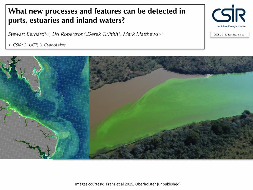
What new processes and features can be detected in ports, estuaries and inland waters? Stewart Bernard1,2, Lisl Robertson2,Derek Griffith1, Mark Matthews2,3 1. CSIR; 2. UCT; 3. CyanoLakes

Images courtesy: Franz et al 2015, Oberholster (unpublished)

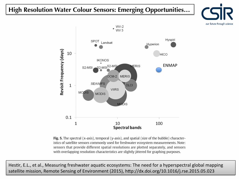
High Resolution Water Colour Sensors: Emerging Opportunities…

atmospheric variability, air–water interface re!ections and refractionfrom diffuse and direct sky and sunlight (Brando & Dekker, 2003;Hochberg et al., 2011; Hu et al., 2012; Wettle, Brando, & Dekker,2004). Another equally important feature of sensor performance forsuccessful measurement of freshwater systems is suf"cient dynamicrange to be able to make sensitive measurements over low radiancepixels (water) while not saturating over neighboring bright pixels(land or sunglint).

The combined effects of SNR anddynamic range impact the accuracyof biophysical retrieval (e.g., Hu et al., 2012; Vanhellemont & Ruddick,2014). For example, when Giardino, Brando, Dekker, Strömbeck andCandiani (2007) used Hyperion to measure CHL and TR in Lake Gardain Northern Italy, they had to convolve a 5 ! 5 low pass "lter over theimage to reduce the effects of the sensor's poor SNR and environmentalnoise (Brando & Dekker, 2003; Wettle et al., 2004), effectively reducingthe spatial resolution from 30m to 150 m. Similarly, Vanhellemont andRuddick (2014) found it necessary to bin Landsat 7 ETM+ data to9 ! 9 pixels (270 m) to reach the noise equivalent of Landsat 8 OLI,and had to further bin the data to 11 ! 11 (330 m) due to the limiteddigitization (8 bits) of Landsat 7 ETM+. Freshwater ecosystems arespatially complex, and typically have both low (water) and high(land) radiance targets in a single scene, making simultaneous mea-surement of both problematic. The high SNR and large dynamic rangeproposed for the HyspIRI mission makes it uniquely well designed formeasuring freshwater ecosystems accurately andmoderate to high spa-tial resolution.

2.7. Current observation capabilities

For every type of measurement, there are tradeoffs in sensor resolu-tion. Fig. 5 shows some of the most common satellite sensors used forfreshwater ecosystem measurements and their relation in terms ofspectral (x-axis), temporal (y-axis), and spatial resolution (size of thebubble). HyspIRI's proposed spectral, temporal and spatial characteris-tics occupy an observation space shared with only a few other satellitemissions. However, HyspIRI's observational capabilities make it uniqueand necessary for freshwater ecosystem measurements, as it occupiesa unique niche in sampling space. Freshwater ecosystemmeasurementsfrom satellite remote sensing can be classi"ed based on the samplingstrategy and frequency. We categorize these different schemes into1) continuous samplers, 2) targeted mappers, and 3) global mappers.Continuous samplers are geostationary satellites that can image hightemporal frequency (e.g., Korea's Ocean Color Satellite GOCI thatmakes a measurement once an hour) of a speci"c location to providenear-continuous monitoring of dynamic processes such as harmfulalgal blooms and river plumes. Continuous samplers provide coarsespatial resolution over a speci"c, targeted region. Targeted mapperscan be considered pseudo global mappers. Also in a lower earth orbit(although not necessarily sun synchronous, e.g., the Hyperspectral Im-ager for the Coastal Ocean, HICO, onboard the International Space Sta-tion), targeted mappers acquire data over particular areas based ondata acquisition requests (e.g., NASA's EO-1 Hyperion or commercialmissions suitable for freshwater like Worldview 2 and 3; WV2, WV3),or regular acquisitions over a region of interest (e.g. the Italian SpaceAgency's proposed PRISMA mission, or the German EnvironmentalMapping and Analysis Program) thatwill providemapping-like capabil-ities over a speci"c region.

Fig. 5 shows the observation capabilities of common current andnear to launch sensors in terms of temporal, spectral, and spatial resolu-tions. Several missions, such as the soon to be launched Sentinel-2Mul-tispectral Instrument (S2-MSI) provide different spectral bands atdifferent pixel resolutions. Thus, while S2-MSI will have 13 spectralbands across the visible, near and shortwave infrared regions, it willonly have four broad “multispectral bands” in the visible and near infra-red regions at 10 meter pixel resolution.

Global mappers are valuable for providing regular, repeated mea-surements of the globe over long periods of time. They typically arealso archivalmissions,meaning they provide a time series of regular ob-servations. Archival global mappers are the most important category ofmeasurement for addressing multiple end user goals of resource moni-toring and ecosystem science. Archival global mapping missions withfree and open data access policies have transformed scienti"c under-standing of earth surface processes (National Research Council, 2007;Wulder et al., 2012), and provide the most valuable datasets for moni-toring (e.g., McCullough, Loftin, & Sader, 2012), and understandingfreshwater ecosystem processes and change (e.g., Olmanson, Brezonik,& Bauer, 2014). While Fig. 5 depicts the observation capabilities of com-mon current and near-ready to launch satellite missions, it includescontinuous and targeted mappers, such as Worldview 2 & 3 and Hype-rion which may not be suited for ecosystem change measurements.Fig. 6 explicitly summarizes the global mapping capability current andnear future global mapping capability for freshwater ecosystem scienceand management. In comparison with current global mapping capabil-ities, HyspIRI occupies a unique measurement space in both its spatialresolution and temporal resolution, and provides signi"cantly morespectral information than any other global mapper (Fig. 6).

3. Case studies

The following case studies illustrate how the characteristics of ahyperspectral global mapping satellite mission, such as the plannedHyspIRI mission, address the needs of freshwater aquatic system scien-tists and managers. We use as our example for freshwater aquatic ecol-ogy the remote sensing of primary producers. In the following casestudies we highlight published data and existing methods, demonstrat-ing thematurity of the science. However, each case study demonstratesexisting gaps in the spatial, temporal, and spectral characteristics of theapplication, highlighting the need of a mission that will "ll these gaps.

3.1. Site description

TheMantua lake system is an important freshwater wetland systeminNorthern Italy that provides critical habitat for aquatic vegetation andwater birds in the region. TheMantua system is formed by the dammingof theMincio River, a tributary of the Po, and fed by Lake Garda, the larg-est lake and longest river of Italy, respectively. The lake waters are

Fig. 5. The spectral (x-axis), temporal (y-axis), and spatial (size of the bubble) character-istics of satellite sensors commonly used for freshwater ecosystem measurements. Note:sensors that provide different spatial resolutions are plotted separately, and sensorswith overlapping resolution characteristics are slightly jittered for graphing purposes.

7E.L. Hestir et al. / Remote Sensing of Environment xxx (2015) xxx–xxx

Please cite this article as: Hestir, E.L., et al., Measuring freshwater aquatic ecosystems: The need for a hyperspectral global mapping satellitemission, Remote Sensing of Environment (2015), http://dx.doi.org/10.1016/j.rse.2015.05.023

HesAr, E.L., et al., Measuring freshwater aquaAc ecosystems: The need for a hyperspectral global mapping satellite mission, Remote Sensing of Environment (2015), hMp://dx.doi.org/10.1016/j.rse.2015.05.023

ENMAP

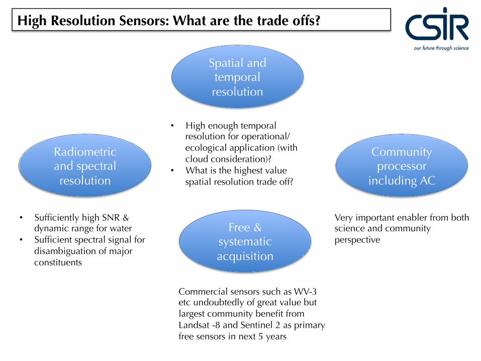
High Resolution Sensors: What are the trade offs?

Radiometric and spectral resolution

Spatial and temporal resolution

Community processor

including AC

Free & systematic acquisition

•  Sufficiently high SNR & dynamic range for water

•  Sufficient spectral signal for disambiguation of major constituents

•  High enough temporal resolution for operational/ecological application (with cloud consideration)?

•  What is the highest value spatial resolution trade off?

Commercial sensors such as WV-3 etc undoubtedly of great value but largest community benefit from Landsat -8 and Sentinel 2 as primary free sensors in next 5 years

Very important enabler from both science and community perspective

!"#$%#&'() &*+ ,+#-'.'$'&/ 01 2/-&+3#&'4 5($#(6 7#&+8 9%#$'&/ :0('&08'() ;'&* 2#&+$$'&+ <+30&+ 2+(-'() = >?

;#&+8 3#(#)+3+(& $+"+$-@ A*+8+ '- # 4$+#8 #"+(%+ 108 '(18#-&8%4&%8+ '("+-&3+(&- #& -&#&+B .#-'(B8+)'0(#$ #(6 $04#$ $+"+$ &*#& ;'$$ -%CC08& &*'- 6+"+$0C3+(& '( -3#8& #(6 +11+4&'"+ '3C$+3+(&#&'0(-@

D (#&'0(#$ $0() &+83 #CC80#4* ;'$$ +(40%8#)+ -&#&+B .#-'(B 8+)'0(#$ #(6 $04#$ $+"+$ 08)#('E#&'0(- &0'("+-& #- &*+/ ;0%$6 +FC+8'+(4+ # $#8)+ 8+&%8( 108 '("+-&3+(&-@ !" #$%&3+#-%8+3+(& 3+&*060$0)'+-G+'&*+8 ./ 1'+$6 -#3C$'() 08 $" #$%& #%&0(030%- '(-&8%3+(&#&'0(H 4#( .+ 40086'(#&+6 &0 -%CC08&I%#(&'&#&'"+ +#8&* 0.-+8"#&'0( '(1083#&'0( #& #$$ -4#$+-@

J@K 7#&+8 I%#$'&/ '(1083#&'0( C806%4&- 108 &*+ (#&'0(#$ -/-&+3A*+ ;#&+8 I%#$'&/ "#8'#.$+- 6'8+4&$/ 3+#-%8+#.$+ '( &*+ ;#&+8 .06/ -%81#4+ $#/+8 G60;( &0 &*+ "'-'.'$'&/ 016+C&*H -%'&#.$+ 108 # (#&'0(#$ 0C+8#&'0(#$ -/-&+3 108 '($#(6 ;#&+8 I%#$'&/ 30('&08'() 1803 +#8&*0.-+8"#&'0( #8+ )'"+( '( A#.$+ J L@

!"#$% & ' (")%* +,"$-). /"*-"#$%0 12* " 3")-23"$ 24%*")-23"$ -3$"35 6")%* +,"$-). 723-)2*-38 0.0)%7 1*27 %"*)92#0%*/")-23

(:!;< =>:?@!A @BCD<E:!@DB (:!;< =>:?@!A F:<@:G?;

H*-7"*. 4*25,I)-23 "35 %,)*249-I")-23 0)"),0 MNO

MPM

MP!

2%81#4+ #$)#$ .$003-

:+,")-I I"*#23 I23)%3)J I"*#23 1$,K%0 MQR:

;*20-23J *% 0,04%30-23 "35 5%420-)-23 A2: G MNOSTDPH

?-89) I$-7")% -312*7")-23 *%$")%5 )2 )9%I27#-3%5 %11%I)0 21 "$8"%J LMDE "350,04%35%5 7"))%*

U6

A8#(-C#8+(4/

A%8.'6'&/

;I2$28-I"$ I235-)-23 !3+8)+(& 3#480C*/&+-

2%.3+8)+6 3#480C*/&+-

MNOV4*$080C*/$$W MPMV4/#(0 C*/404/#('(W MP!V4/#(0 C*/40+8/&*8'(BMQR:V40$0%8+6 6'--0$"+6 08)#('4 3#&&+8W A2: &0&#$ -%-C+(6+6 3#&&+8WTDPV(0( #$)#$ C#8&'4%$#&+ 3#&&+8W U6V"+8&'4#$ #&&+(%#&'0( 01 $')*&

X/ #--'3'$#&'() +#8&* 0.-+8"#&'0( 6+8'"+6 ;#&+8 I%#$'&/ '(1083#&'0( ;'&* Y Q */6806/(#3'4 #(6.'0)+04*+3'4#$ 306+$-B 6+C&* 8+-0$"+6 #--+--3+(&- '( *'(64#-& #(6 (0;4#-& 1083 4#( .+ 3#6+ #- ;+$$ #-C8+6'4&'0(- 01 &*+-+ '(&+)8#&+6 #--+--3+(&-@ A*+ 3+&*060$0)/ &0 &*'- 6#&# #--'3'$#&'0( '- '( 6+"+$0C3+(&#(6 ;'$$ C80"'6+ '3C80"+6 %(6+8-&#(6'() #(6 3#(#)+3+(& 8+$+"#(& C8+6'4&'0( &00$-@

7#&+8 -%81#4+ &+3C+8#&%8+ '(1083#&'0( 4#( .+ #66+6 &0 &*'- -%'&+ 01 '(1083#&'0( 1803 +#8&* 0.-+8"'()-+(-08- &0 '3C80"+ %(6+8-&#(6'() 01 &*+83#$ 400$'() G6++C ;#&+8 8+-+8"0'8 0%&$+&-H 08 &*+83#$ *+#&'()@

5( &*+ (+F& -+4&'0( &*+ -#&+$$'&+ -+(-08- #"#'$#.$+ 108 8+&80-C+4&'"+B 4%88+(& #(6 1%&%8+ '($#(6 ;#&+8 I%#$'&/6+&+4&'0( #(6 30('&08'() #8+ 6'-4%--+6 '( &*+ 40(&+F& 01 .0%(6#8/ 40(6'&'0(- '( 6+"+$0C'() # (#&'0(#$'($#(6 ;#&+8 I%#$'&/ 30('&08'() -/-&+3 %-'() +#8&* 0.-+8"#&'0(@ A*+/ #8+ 6'-4%--+6 '( # -+I%+(4+ &*#&#$')(- ;'&* &*+ C80C0-+6 *'+8#84*'4#$ 18#3+;08Z 01 20! #(6 T79D-[ 1803 -&#&+ 08 8'"+8 .#-'( &0 8+)'0(#$#(6 $04#$ ;#&+8 3#(#)+3+(& 8+C08&'() $+"+$-@

,803 &*+ (#&'0(#$ &0 $04#$ -4#$+ &*+ -+(-08- 30-& -%'&#.$+ ;0%$6 .+ &*+ $0; -C#&'#$B *')* &+3C08#$8+-0$%&'0( +#8&* 0.-+8"#&'0( -+(-08- G30-& -%'&#.$+ 108 (#&'0(#$ $+"+$ 8+C08&'()HB "'# 3+6'%3 -C#&'#$ #(6&+3C08#$ 8+-0$%&'0( G-%'&#.$+ 108 (#&'0(#$ &0 8'"+8 .#-'( #(6 -&#&+ #(6 8+)'0(#$ $+"+$ 8+C08&'()H &0 *')*-C#&'#$ 8+-0$%&'0( -+(-08- -%'&#.$+ 108 6+&#'$+6 $+"+$ 8+C08&'()@

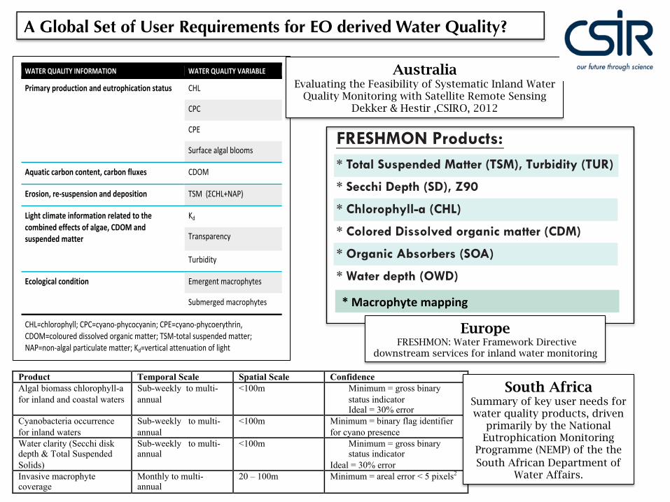
Product! Temporal Scale! Spatial Scale! Confidence!Algal biomass chlorophyll-a for inland and coastal waters!

Sub-weekly to multi-annual!

<100m! Minimum = gross binary status indicator!Ideal = 30% error!

Cyanobacteria occurrence for inland waters!

Sub-weekly to multi-annual!

<100m! Minimum = binary flag identifier for cyano presence!

Water clarity (Secchi disk depth & Total Suspended Solids)!

Sub-weekly to multi-annual! <100m! Minimum = gross binary

status indicator!Ideal = 30% error!

Invasive macrophyte coverage! Monthly to multi-

annual! 20 – 100m! Minimum = areal error < 5 pixels2!!

South Africa Summary of key user needs for water quality products, driven

primarily by the National Eutrophication Monitoring

Programme (NEMP) of the the South African Department of

Water Affairs.

Australia Evaluating the Feasibility of Systematic Inland Water

Quality Monitoring with Satellite Remote Sensing Dekker & Hestir ,CSIRO, 2012

!"#$%&'()%*$+(,-'+..*'+("+'"*+/+$(-0%-'*&(1"#1+"'*+2

345,6789

345,6789(1"#:+&'($+2&"*1'*#;<(!"#$%&'()*+),-)#.)/011,203,4*56)73086/4)+64)97)40)7305*:6)%*;<)"6+0=194*0-)!"#$%>,463)&'(*403*-;),-:)?0>-+436,@)$635*/6+A)B<6)@,*-)02=86/4*56)*+)40)/36,46)/0-4*-909+),-:)>611),//6746:):0>-+436,@)+635*/6+)C03)*-1,-:)>,463)@0-*403*-;),4)#93076,-)16561A)B<6)73086/4)DEFGF=EFGHI)*+)C9-:6:)2J)4<6)#93076,-).-*0-)9-:63)4<6)K4<)!3,@6>03L)M30;3,@@6)D73086/4)-9@263)ENHEOKIA

345,6789(!"#$%&'2<=(>#'-.(,%21+;$+$(7-''+"(?>,7@A(>%"B*$*'C(?>D4@

=(,+&&E*(F+1'E(?,F@A(GHI

=(JE.#"#1EC..K-(?J6L@

=(J#.#"+$(F*22#./+$(#")-;*&(M-''+"(?JF7@

=(8")-;*&(NB2#"B+"2(?,8N@

=(O-'+"($+1'E(?8OF@

!"#:+&'(1-"';+"2<

4+P+"+;&+(!"#:+&'2<

M16,+6)5*+*4)093)>62+*46PQQQRP"+2EM#;R+%

!"#$%&'()*+,"-$((./0"

Europe FRESHMON: Water Framework Directive

downstream services for inland water monitoring

A Global Set of User Requirements for EO derived Water Quality?

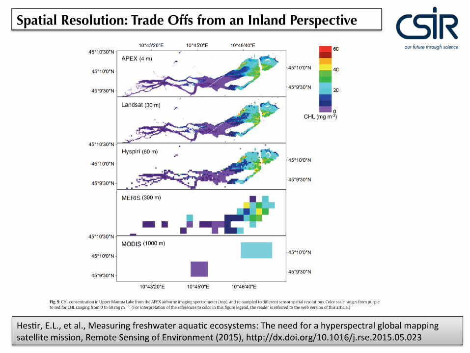
Based on our estimates of freshwater ecosystem observability inSection 2.4 (Fig. 4), Lake Mantua is not observable by either MODIS orMERIS, because there is not a 4 ! 4 block of pixels contained withinthe boundary of the water body (Fig. 9). This case study of LakeMantuaillustrates how the often sinuous, riverine shape and spatial complexity

of freshwater systems in!uence their observability. While there areMERIS pixels presentwithin thewater body in Fig. 9, a close comparisonof the edges of thewater body as resolved by APEX show that theMERISpixels are mixed with adjacent land and wetland complex pixels. Thelarge levee bisecting the upper northeast portion of lake and the wet-land stream complex in the southwest portion of the lake are not re-solved at all by MERIS. At the MODIS pixel resolution, there are nopixels that do not contain signi"cant portions of land.

Recently it was suggested that while large spatial resolution sensorssuch as MODIS and MERIS could not effectively view the majority offreshwater systems, they could be used to measure a selection ofwater bodies representative of a target ecosystem, serving as “virtualstations” for ecosystem measurement (Dekker & Hestir, 2012). Theseresults challenge that suggestion because a lake that is only resolvedby a few large pixels results in a “smoothing” of the CHLmeasurements;local areas of high concentration are mixed with areas of lower concen-tration to produce results thatmaybe indicative of the “average” surfaceconcentration, but may not be informative to interpreting spatial pat-terns in the data. For example, the large pixels representing “average”surface concentration conditions could impede algal bloom detection,and may obfuscate sources of eutrophication and processes of primaryproduction. In such an instance, using MERIS measurements as virtualstations for ecological understanding of Lake Mantua may be toolimited.

Fig. 8. Seasonal variation inWAVI (averages and standard deviations) from Landsat 8 OLIfor 5 different aquatic vegetation communities and open water.

CHL (mg m-3)

(4 m)

(30 m)

(60 m)

(300 m)

(1000 m)

Fig. 9. CHL concentration inUpperMantua Lake from the APEX airborne imaging spectrometer (top), and re-sampled to different sensor spatial resolutions. Color scale ranges from purpleto red for CHL ranging from 0 to 60 mg m!3. (For interpretation of the references to color in this "gure legend, the reader is referred to the web version of this article.)

10 E.L. Hestir et al. / Remote Sensing of Environment xxx (2015) xxx–xxx

Please cite this article as: Hestir, E.L., et al., Measuring freshwater aquatic ecosystems: The need for a hyperspectral global mapping satellitemission, Remote Sensing of Environment (2015), http://dx.doi.org/10.1016/j.rse.2015.05.023

Spatial Resolution: Trade Offs from an Inland Perspective

HesAr, E.L., et al., Measuring freshwater aquaAc ecosystems: The need for a hyperspectral global mapping satellite mission, Remote Sensing of Environment (2015), hMp://dx.doi.org/10.1016/j.rse.2015.05.023

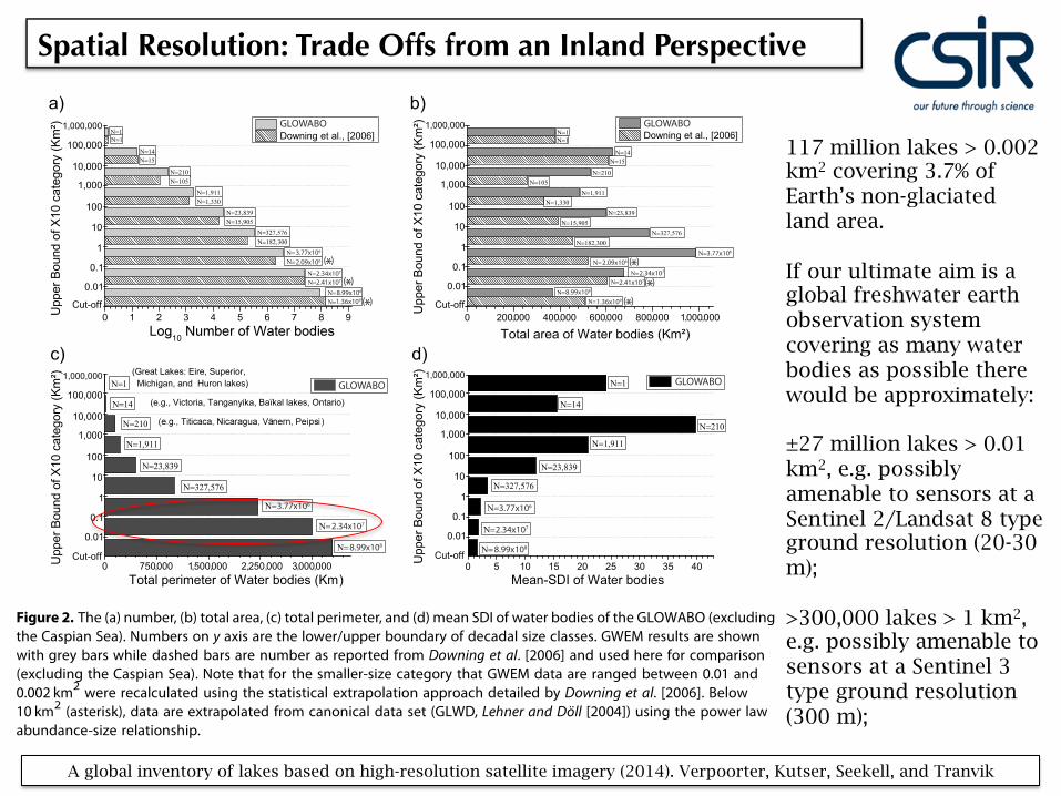
117 million lakes > 0.002 km2 covering 3.7% of Earth’s non-glaciated land area. If our ultimate aim is a global freshwater earth observation system covering as many water bodies as possible there would be approximately: ±27 million lakes > 0.01 km2, e.g. possibly amenable to sensors at a Sentinel 2/Landsat 8 type ground resolution (20-30 m); >300,000 lakes > 1 km2, e.g. possibly amenable to sensors at a Sentinel 3 type ground resolution (300 m);

A global inventory of lakes based on high-resolution satellite imagery (2014). Verpoorter, Kutser, Seekell, and Tranvik

3. Global Abundance and Distribution of Lakes

The database contains about 27 million water bodies larger than 0.01 km2 with a total surface area of4.76 ! 106 km2 excluding Caspian Sea (Figure 2). This is approximately 3.5% of Earth’s nonglaciated landsurface area. About 22 million water bodies larger than 0.01 km2 are located between 60°N and 56°S,where elevation data are available. These lakes have a total surface area of 1.89 ! 106 km2, 1.4% ofnonglaciated land surface area. Hence, about 5 million lakes north of 60°N or south of 56°S, where thereare no digital elevation data, make up a substantial fraction of the global lake area. There are about117 million lakes greater than 0.002 km2, covering a total area of 5.0 ! 106 km2, which corresponds to 3.7%of Earth’s nonglaciated land surface. Accordingly, about 90 million lakes in the smallest size bin (0.002to 0.01 km2) make up only 0.27% of the nonglaciated land surfaces, which is mostly dominated by lakeslarger than 0.01 km2.

The highest concentration, area, and perimeter of water bodies appear at boreal and arctic latitudes (45°–75°N).Water body abundance is lower at southern latitudes where the continental area is also lower. The generalpattern is consistent with previously published map compilations [Lehner and Döll, 2004], albeit with morevariability (Figures 3a, 3c, and 3e). Size distribution of water bodies decreases drastically across elevationwhere 85% of lakes, 50% of lake area, and 50% of total lake perimeter are located at elevations lower than500m above sea level (Figures 3b, 3d, and 3f).

The total area contributed by decadal water body size categories increases with the decreasing size down toan area of 0.1 km2 (Figure 2a). This pattern is consistent with previously reported results based on mapcompilations and statistical extrapolations [Downing et al., 2006]. However, the area of lakes< 0.1 km2 is lessand does not follow the pattern of larger lakes. This result is inconsistent with prevailing knowledge derivedfrom statistical extrapolations. Water bodies smaller than 0.1 km2 are numerous, but they contribute only

Figure 2. The (a) number, (b) total area, (c) total perimeter, and (d) mean SDI of water bodies of the GLOWABO (excludingthe Caspian Sea). Numbers on y axis are the lower/upper boundary of decadal size classes. GWEM results are shownwith grey bars while dashed bars are number as reported from Downing et al. [2006] and used here for comparison(excluding the Caspian Sea). Note that for the smaller-size category that GWEM data are ranged between 0.01 and0.002 km2 were recalculated using the statistical extrapolation approach detailed by Downing et al. [2006]. Below10 km2 (asterisk), data are extrapolated from canonical data set (GLWD, Lehner and Döll [2004]) using the power lawabundance-size relationship.

Geophysical Research Letters 10.1002/2014GL060641

VERPOORTER ET AL. ©2014. The Authors. 3

Spatial Resolution: Trade Offs from an Inland Perspective

High Resolution Sensors: Need for High Quality Radiometry

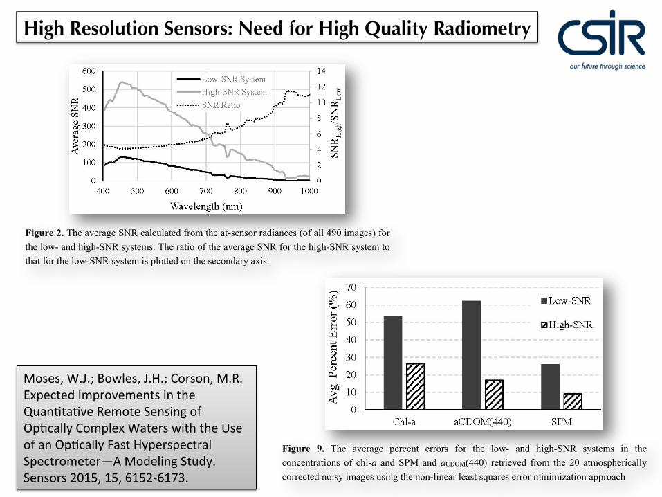
Moses, W.J.; Bowles, J.H.; Corson, M.R. Expected Improvements in the QuanAtaAve Remote Sensing of OpAcally Complex Waters with the Use of an OpAcally Fast Hyperspectral Spectrometer—A Modeling Study. Sensors 2015, 15, 6152-‐6173.

!"#$%&$'!"#$!"()' %#$&""

"

#$%$&%'(")%"*)+$,$-.%/0"1$,'*"234"-5")-#")1'+$"634"-5")-#",'*$("%/)-"%/)%"'7"%/$"89:;"#$%$&%'(")%"*)+$,$-.%/0"1$%*$$-"234"-5")-#"634"-5<"=/$"0%)-#)(#"#$+>)%>'-"'7")"#)(?">5).$")&@A>($#"1B"89:;"*)0"%)?$-"%'"($C($0$-%"%/$"&'51>-)%>'-"

'7"#)(?"-'>0$!"($)#'A%"-'>0$!")-#"#>.>%>D)%>'-"-'>0$"7'("%/$",'*EFGH"0B0%$5<"I'("%/$"/>./EFGH"0B0%$5!"%/$"#)(?"-'>0$!"($)#'A%"-'>0$!")-#"#>.>%>D)%>'-"-'>0$"*$($"'1%)>-$#"7('5"%/$">-7'(5)%>'-"0/$$%"7'("%/$""IJKELML3N":O;F"#$%$&%'(<"9-"&/)-.>-." %/$"IE-A51$("7('5"P<3" %'"Q<4"*/>,$"5)>-%)>->-." %/$"7'&)," ,$-.%/!" %/$"#>)5$%$("'7" %/$"

)C$(%A($" *)0" >-&($)0$#" 1B" P<3" %>5$0!" ($0A,%>-." >-" )" QL<L3E7',#" >-&($)0$" >-" %/$" )($)" '7" %/$" )C$(%A($<""=/A0!" )" 0B0%$5" *>%/" IE-A51$(" R" Q<4" ($&$>+$0" QL<L3" %>5$0" 5'($" C/'%'-0" %/)-" )" 0B0%$5" *>%/""IE-A51$("R"P<3!",$)#>-."%'")"0>.->7>&)-%">5C('+$5$-%">-"%/$"FGH<"=/>0">0">,,A0%()%$#">-"I>.A($"L!"*/>&/"&'-%)>-0"C,'%0"'7"%/$")+$().$"FGH"&),&A,)%$#"7('5"%/$")%E0$-0'("()#>)-&$0"7'("),,"2S4">5).$0"7'("1'%/"0B0%$50<"=/$")+$().$"FGH"7'("%/$"/>./EFGH"0B0%$5"TIE-A51$("R"Q<4U">0"5'($"%/)-"7'A("%>5$0"/>./$("%/)-"%/$")+$().$"FGH"7'("%/$",'*EFGH"0B0%$5"TIE-A51$("R"P<3U"%/('A./'A%"%/$"+>0>1,$"0C$&%(),"()-.$!"*/$($"0/'%"-'>0$"#'5>-)%$0!")-#"AC"%'"Q4VQL"%>5$0"/>./$(">-"%/$"G9H"($.>'-!"*/$($"%/$"#)(?"-'>0$")-#"($)#"-'>0$"C,)B")"#'5>-)-%"(',$<"

"

'()*+,-!."=/$")+$().$"FGH"&),&A,)%$#"7('5"%/$")%E0$-0'("()#>)-&$0"T'7"),,"2S4">5).$0U"7'("%/$",'*E")-#"/>./EFGH"0B0%$50<"=/$"()%>'"'7"%/$")+$().$"FGH"7'("%/$"/>./EFGH"0B0%$5"%'"%/)%"7'("%/$",'*EFGH"0B0%$5">0"C,'%%$#"'-"%/$"0$&'-#)(B")W>0<""

L<P<P<"95C('+>-."X77$&%>+$"FGH"%/('A./"Y'0%EY('&$00>-."

9-" )##>%>'-" %'"5)?>-."&/)-.$0" %'" %/$" 0$-0'(" &'-7>.A()%>'-!" %/$"A-&$(%)>-%B" >-" %/$" )%5'0C/$(>&),,B"&'(($&%$#"#)%)"&)-"1$"7A(%/$("($#A&$#"1B"C'0%EC('&$00>-."5$%/'#0<"I'(">-0%)-&$!"%/$"-'>0$">-"%/$"G9H"0C$&%(),"1)-#0"A0$#"7'(")%5'0C/$(>&"&'(($&%>'-"&)-"1$"($#A&$#"1B")+$().>-."%/$"C>W$,0">-"%/$"0C)%>),"'("0C$&%(),"#'5)>-0<"FA&/")+$().>-.!"*/$-"C$(7'(5$#")%"($)0'-)1,B"5'#$()%$"0&),$0!"*>,,"/)+$"-$.,>.>1,$">5C)&%" '-" #)%)" )-),B0>0" 1$&)A0$" %/$" ($7,$&%)-&$0" )%" %/$0$" 0C$&%()," 1)-#0" T1$B'-#"634"-5U" )($" '7%$-"A0$#" C(>5)(>,B" 7'(" )%5'0C/$(>&" &'(($&%>'-" '-,B" )-#" -'%" 7'(" ($%(>$+>-." *)%$(" @A),>%B" C)()5$%$(0<"8'*$+$(!" 0C)%>)," )+$().>-." >0" C($7$(($#" '+$(" 0C$&%()," )+$().>-." 1$&)A0$" 0C$&%()," )+$().>-.!" */>,$">-&($)0>-."%/$"FGH!"*>,,"&')(0$-"%/$"0C$&%(),"($0',A%>'-")%"0C$&%(),"1)-#0"%/)%")($"A0$#"7'("%/$"($%(>$+),"7'(" )%5'0C/$(>&" C)()5$%$(0Z" 0C)%>)," )+$().>-."*>,," -'%" /)+$" )" #$%(>5$-%)," $77$&%" '-" %/$" ($%(>$+)," '7"

!"#$%&$'!"#$!"()' %#%&""

"

"

'()*+,- ./" #$%" &'%(&)%" *%(+%,-" %((.(/" 0.(" -$%" 1.23" &,4" $5)$3678" /9/-%:/" 5," -$%"+.,+%,-(&-5.,/" .0" +$13*" &,4" 6;<" &,4"*=>?<@AABC" (%-(5%'%4" 0(.:" -$%" DB" &-:./*$%(5+&119"+.((%+-%4",.5/9"5:&)%/"E/5,)"-$%",.,315,%&("1%&/-"/FE&(%/"%((.(":5,5:5G&-5.,"&**(.&+$"

@55C"6%:53H,&19-5+&1"7I83(%4"H1).(5-$:J"

#$%"-2.3K&,4"7I83(%4"&1).(5-$:"5/",.-"+.:*E-&-5.,&119"5,-%,/5'%"&,4"2&/"-$%(%0.(%"&**15%4"-."&11"ALB"5:&)%/M"N5)E(%"OB"/$.2/"-$%"&'%(&)%"*%(+%,-"%((.(/".0"-$%"%/-5:&-%4"+$13*"+.,+%,-(&-5.,/"0.("-$%"1.23" &,4" $5)$3678" /9/-%:/" 25-$" &,4" 25-$.E-" /*&-5&1" &'%(&)5,)" &-" 7I8" 2&'%1%,)-$/M" #$%" &'%(&)%"*%(+%,-" %((.(" 0.(" -$%" 1.23678" /9/-%:"2&/" '%(9" $5)$" @AOBMODPCM" H1).(5-$:/" /E+$" &/" -$%" -2.3K&,4"7I83(%4" &1).(5-$:" -$&-" &(%" %:*5(5+&119" *&(&:%-%(5G%4" &(%" '%(9" /%,/5-5'%" -." -$%" +.%005+5%,-/" .0" -$%"(%)(%//5.," %FE&-5.," ).'%(,5,)" -$%" &1).(5-$:M" #$%/%" &1).(5-$:/" &(%" KE51-" .," -$%" &//E:*-5.," -$&-"'&(5&-5.,/"5,"-$%"(%01%+-&,+%/"&-"-$%"2&'%1%,)-$/"5,+1E4%4"5,"-$%"&1).(5-$:"&(%"*(5:&(519!"50",.-"/.1%19!"4E%"-."'&(5&-5.,/"5,"-$%"2&-%("FE&15-9"*&(&:%-%(".0"5,-%(%/-M"H/"/E+$!"-$%/%"&1).(5-$:/"&(%"'%(9"/%,/5-5'%"-."'&(5&-5.,/"5,"-$%"(%01%+-&,+%/"4E%"-."&,9".-$%("0&+-.("/E+$"&/"/%,/.(",.5/%M"#$5/"5/"5:*.(-&,-"-."K%&("5,":5,4"2$%,"&//%//5,)"-$%"7I83(%4"&1).(5-$:"K%+&E/%"-$%"%00%+-/".0"-$%"/%,/.(",.5/%"&(%"%Q*%+-%4"-."K%"$5)$%(" 5," -$%" 1.,)%("2&'%1%,)-$/M"#$%",E:%(5+&1":%-$.4!".," -$%".-$%("$&,4!" +.,/54%(/" -$%" %,-5(%"/*%+-(E:"2$51%"(%-(5%'5,)"2&-%("FE&15-9"*&(&:%-%(/"@ABBRSDT",:"5,".E("+&/%C"&,4"+&,"-%,4"-."&'%(&)%".E-" -$%" ,.5/%" &+(.//" -$%" /*%+-(E:" 25-$.E-" K%5,)" .'%(19" /%,/5-5'%" -." ,.5/%" 5," .,%" .(" -2." *&(-5+E1&("2&'%1%,)-$/M"#$%"&K/.1E-%"%((.("95%14%4"K9"&"/%:53&,&19-5+&1"&1).(5-$:"+&,"K%":5-5)&-%4"K9"&4UE/-5,)"-$%"+.%005+5%,-/".0"-$%"(%)(%//5.,"%FE&-5.,M"#$%"%:*$&/5/"$%(%"5/!"-$%(%0.(%!",.-".,"-$%"&K/.1E-%"%((.("5,"-$%" +$13*" +.,+%,-(&-5.,/" (%-(5%'%4" 0(.:" -$%"7I83(%4" &1).(5-$:"KE-" .," -$%" 5:*(.'%:%,-" &+$5%'%4" K9"/*&-5&119"&'%(&)5,)"-$%"7I8"(%01%+-&,+%/"&,4"+$&,)5,)"-$%"N3,E:K%(M"V$%,"7I8"(%01%+-&,+%/"0(.:"-$%"1.23678"/9/-%:"2%(%"/*&-5&119"&'%(&)%4!"-$%"*%(+%,-"%((.("5,"-$%"(%-(5%'%4"+$13*"+.,+%,-(&-5.,"(%4E+%4"-."OLDMWLPM"#$%"*%(+%,-" %((.(" 0.(" -$%"$5)$3678"/9/-%:"2&/"XDMBYP"25-$.E-"7I8"/*&-5&1" &'%(&)5,)"&,4"OYMWYP"25-$"/*&-5&1"&'%(&)5,)"&-" -$%"7I8"/*%+-(&1"K&,4/M" I,"/E::&(9!" -$%"%((.(" 5," -$%" (%-(5%'%4"+$13*" +.,+%,-(&-5.," (%4E+%4" K9" LDMOWP"2$%," -$%" N3,E:K%("2&/" +$&,)%4" 0(.:"XMT" -." OMBM" N.(" K.-$"/9/-%:/!"/*&-5&1"&'%(&)5,)"5,"-$%"7I8"2&'%1%,)-$/"(%/E1-%4"5,"&**(.Q5:&-%19"TBP"(%4E+-5.,"5,"%((.("5,"-$%"(%-(5%'%4"+$13*"+.,+%,-(&-5.,M"

400 500 600 700 800 9000

0.005

0.01

0.015

L w R

efle

ctan

ce a

t TO

A

400 500 600 700 800 9000

20

40

60

SNR

on

L w a

t TO

A

Wavelength [nm]

Hy011Mod003L8 : Water−leaving Refl. at TOA with SNR M10/0/1/0.1/0.5 with HiVis/UrbAer/LoVap/NoCld/HiAdjGrn

400 500 600 700 800 9000

1

2

x 10−3

L w R

efle

ctan

ce a

t TO

A

400 500 600 700 800 9000

5

10

SNR

on

L w a

t TO

A

Wavelength [nm]


400 500 600 700 800 9000

0.01

0.02

L w R

efle

ctan

ce a

t TO

A

400 500 600 700 800 9000

20

40

SNR

on

L w a

t TO

A

Wavelength [nm]


400 500 600 700 800 9000

0.2

0.4

0.6

0.8

1

1.2

x 10−3

L w R

efle

ctan

ce a

t TO

A

400 500 600 700 800 9000

1

2

3

4

5

6

SNR

on

L w a

t TO

A

Wavelength [nm]


400 500 600 700 800 9000

1

2

x 10−3

L w R

efle

ctan

ce a

t TO

A

400 500 600 700 800 9000

5

10

SNR

on

L w a

t TO

A

Wavelength [nm]


Chl=1 mg m-3 Case 1

Chl=10 mg m-3 Case 1

Chl=10 mg m-3 High scattering


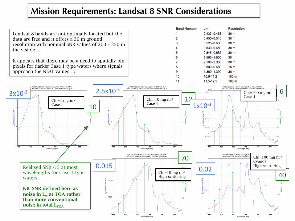
Landsat 8 bands are not optimally located but the data are free and it offers a 30 m ground resolution with nominal SNR values of 200 – 350 in the visible…. It appears that there may be a need to spatially bin pixels for darker Case 1 type waters where signals approach the NEΔL values….

Realised SNR < 5 at most wavelengths for Case 1 type waters NB: SNR defined here as noise in Lw at TOA rather than more conventional noise in total LTOA

10 10

3x10-‐3 2.5x10-‐3 3x10-‐3

1x10-‐3

0.015 0.02

6

40

70 Chl=100 mg m-3 Cyanos High scattering

Mission Requirements: Landsat 8 SNR Considerations

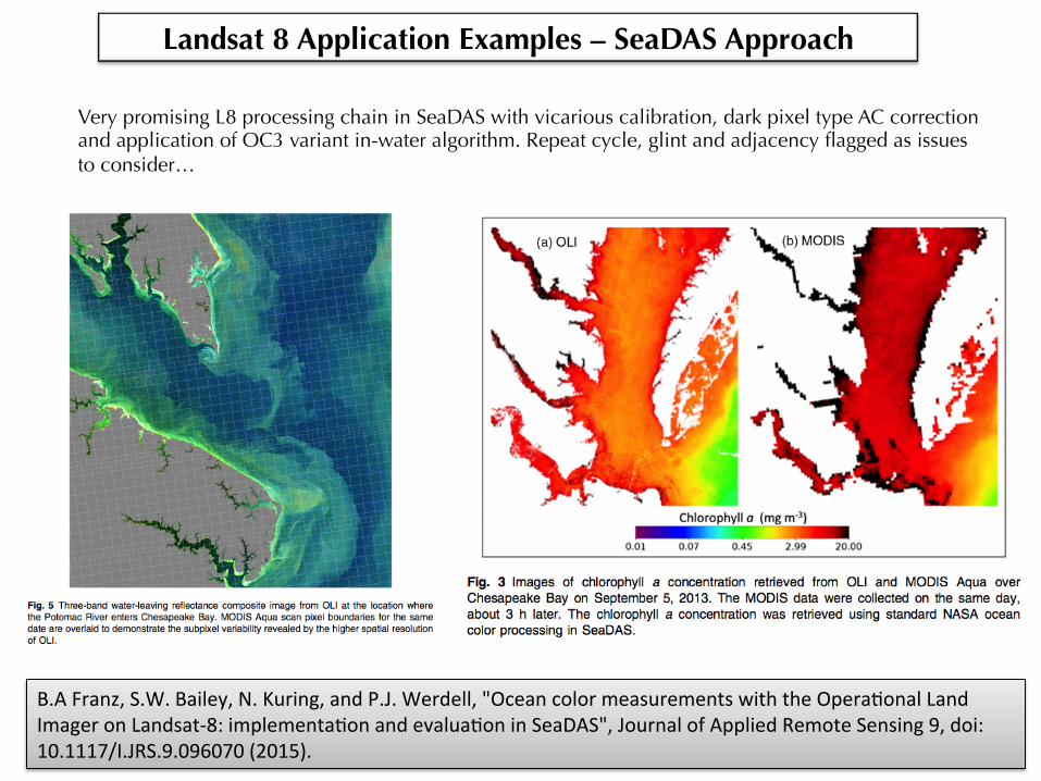
B.A Franz, S.W. Bailey, N. Kuring, and P.J. Werdell, "Ocean color measurements with the OperaAonal Land Imager on Landsat-‐8: implementaAon and evaluaAon in SeaDAS", Journal of Applied Remote Sensing 9, doi:10.1117/I.JRS.9.096070 (2015).

Landsat 8 Application Examples – SeaDAS Approach

Very promising L8 processing chain in SeaDAS with vicarious calibration, dark pixel type AC correction and application of OC3 variant in-water algorithm. Repeat cycle, glint and adjacency flagged as issues to consider…

!"#$%&'()*+$%,-'."&%/'$0'1&%,2'34/"%5&,6$7897:"%/,&7:67;'&'<2&7;67;'=$%>:'?$5"@4"%'(A*(BC'DE((' 'F"%7:$7C'G6%;676&'

H9IIJK.''

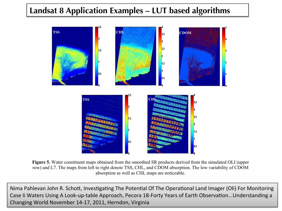
This paper examined the applicability of the new generation of Landsat sensors (OLI) in water quality studies. With its enhanced features including higher SNR, increased radiometric fidelity, and the addition of a short blue band centered at 440 nm, OLI enables obtaining water constituent maps superior to those derived from the existing Landsat (L7). This was demonstrated via a LUT approach where a physics-based model was used to simulate water-leaving reflectances for various combinations of water constituents. The surface reflectance products were compared against those derived from MODIS and simulations. The retrieved chlorophyll maps were validated with a MODIS-derived chlorophyll distribution map and the errors were reported. The concentrations of suspended solids, however, measured in the river/river mouth were utilized to validate the TSS concentration maps. The results showed that OLI is capable of retrieving high-fidelity CHL maps with respect to L7 primarily due to its CA band.'

In addition, as expected, this band allows for mapping CDOM absorption throughout clear waters at low

CHL/TSS concentrations. Nevertheless, the TSS maps derived from L7 are reasonably comparable to that of OLI even though L7 tends to overestimate the concentrations. This overestimation is attributed to the calibration issues associated with L7’s red band which, along with the green band, exhibits a strong correlation with the TSS concentrations. In addition, the low radiometric fidelity of L7 contributes to the overestimation of the concentrations in the proposed LUT approach. The higher concentration levels are on the order of 10.5% relative to OLI data. In order to more realistically evaluate OLI’s potential in such studies, the SR products were smoothed to improve the SNR resembling the desired design specification. The constituent maps derived from the enhanced SNR products appear to remove local variability of the concentration maps, in particular of the CHL maps. The produced error maps assisted in verifying the robustness of the IOPs and the atmospheric compensation technique. The error levels throughout the plume area turn out to be less than 3% and 5% for OLI and L7, respectively.

It should be noted that in this study the differences in the acquisition geometries were not taken into account. It is believed that this difference introduces a negligible error in the constituent retrieval process. The present study will be further extended by examining the retrieved constituent maps against the Hyperion-derived maps as a best-

LHH' <FM' <N3I'

LHH' <FM'

+6;O%"'PQ Water constituent maps obtained from the smoothed SR products derived from the simulated OLI (upper row) and L7. The maps from left to right denote TSS, CHL, and CDOM absorption. The low variability of CDOM

absorption as well as CHL maps are noticeable.

Nima Pahlevan John R. SchoM, InvesAgaAng The PotenAal Of The OperaAonal Land Imager (Oli) For Monitoring Case Ii Waters Using A Look-‐up-‐table Approach, Pecora 18-‐Forty Years of Earth ObservaAon...Understanding a Changing World November 14-‐17, 2011, Herndon, Virginia

Landsat 8 Application Examples – LUT based algorithms

!Lc ! !L

am !Lw ! 0

! ""7#

where!ci is the Rayleigh corrected re!ectance, !ami the multiple scatteringaerosol re!ectance, ti the atmospheric transmittance, and !wi themarinere!ectance in band i. The L superscript refers to the SWIR band used inthe correction, band 6 or 7. The aerosol type, "5,L, is considered constant

over the scene and can be determined from clear water pixels as theslope of the regression line !cL vs !c5 or the median of the !cL : !c5 ratio.Herewe again use themedian, as it allows for amore robust determina-tion, relatively insensitive to outliers. Clear water pixels were selectedby constraining the data to pixels where:

!Lc $ 0:005

!5c

N0:8: "8#

Fig. 1.Rayleigh corrected RGB (channels 4–3–2) OLI image over Belgian coastalwaters (2014-03-16, scene LC81990242014075LGN00), showing turbid coastalwaterswith high sedimentconcentration (yellow-brown). The circle shows dumping of dredgedmaterial at a designated site (other example in Fig. 13 and (Vanhellemont & Ruddick, 2014b), see zoomed version inFig. 2).

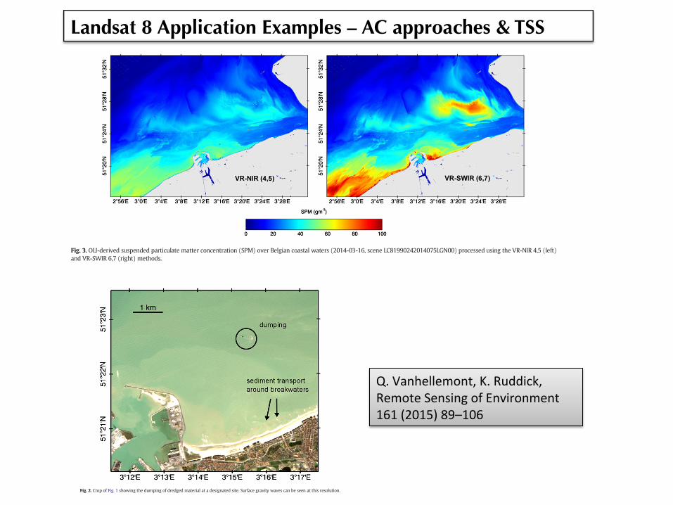
Fig. 2. Crop of Fig. 1 showing the dumping of dredged material at a designated site. Surface gravity waves can be seen at this resolution.

92 Q. Vanhellemont, K. Ruddick / Remote Sensing of Environment 161 (2015) 89–106

Eq. (8) excludes turbid waters by removing pixels where the NIR re-!ectance is higher thanwhat is expected from the aerosol re!ectance inband L. The offset of 0.005 is included to retain low re!ectance pixelswhere the ratio threshold is too restrictive. !w5 can then be computedusing:

!5w ! 1

t5!5c!"5;L!L

am

! ": "9#

In the case of using the two SWIR bands, "6,7 is easily calculated from!c6 and !c7, which are assumed to have zero marine contributions. Apixel-by-pixel "6,7 can be computed, or a single value per scene can beestimated from !c7, !c6, using the median ratio or regression slope. Theformer allows for spatially varying aerosols, the latter minimizes impactof noise in the SWIR bands.

Spectral " is derived using the simple exponential extrapolation(Gordon & Wang, 1994):

"i;L ! "S;L! "#i

"10#

where L and S are the longest (5, 6 or 7) and shortest (4, 5 or 6) wave-length bands used, and

#i ! $L!$i

$L!$S"11#

!w at other wavelengths can then be derived from !c:

!iw ! 1

ti!ic!"i;L $ !L

am

! ": "12#

At present insuf"cient in situ data are available for the validation ofOLI products, although a preliminary validation using Aeronet-OC data(Zibordi et al., 2009) was performed by (Vanhellemont, Bailey, Franz,& Shea, 2014), showing good agreement between OLI and in situ spec-tra. In this study, imagery from the well-established Moderate Resolu-tion Spectroradiometers (MODIS) on the Aqua and Terra platforms areused for the validation. The closest available (same day) L1A sceneswere selected and processed to L2 using SeaDAS version 7.0.2. Imageswere processed at 250 m resolution using the Gordon and Wang

Fig. 3. OLI-derived suspended particulate matter concentration (SPM) over Belgian coastal waters (2014-03-16, scene LC81990242014075LGN00) processed using the VR-NIR 4,5 (left)and VR-SWIR 6,7 (right) methods.

Fig. 4.Multiple scattering aerosol re!ectance at 865 nm(!am5 ) from the 2014-03-16 image over Belgian coastal waters (2014-03-16, scene LC81990242014075LGN00) processed using theVR-NIR 4,5 (left) and VR-SWIR 6,7 (right) methods.

93Q. Vanhellemont, K. Ruddick / Remote Sensing of Environment 161 (2015) 89–106Landsat 8 Application Examples – AC approaches & TSS

Q. Vanhellemont, K. Ruddick, Remote Sensing of Environment 161 (2015) 89–106

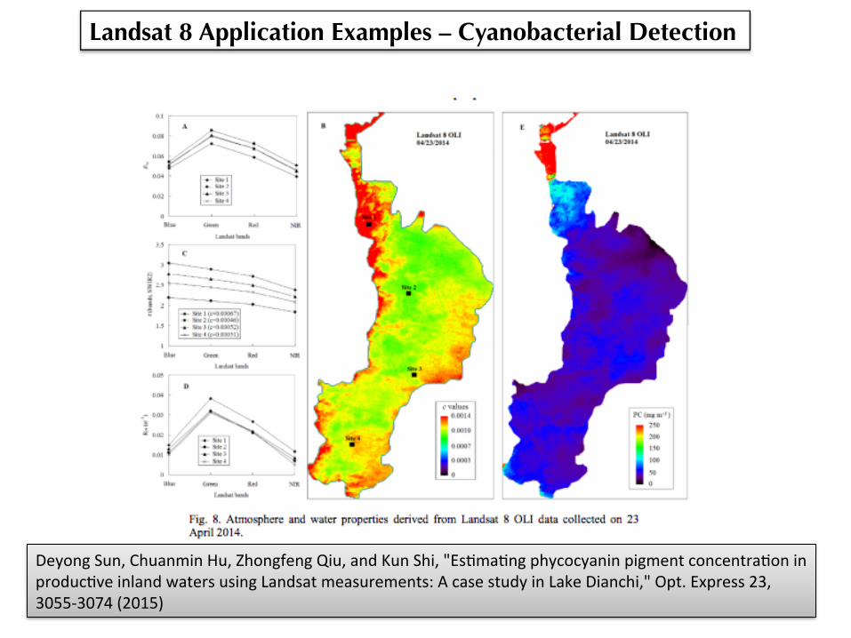
Deyong Sun, Chuanmin Hu, Zhongfeng Qiu, and Kun Shi, "EsAmaAng phycocyanin pigment concentraAon in producAve inland waters using Landsat measurements: A case study in Lake Dianchi," Opt. Express 23, 3055-‐3074 (2015)

Landsat 8 Application Examples – Cyanobacterial Detection

400 500 600 700 800 9000

0.5

1

1.5

2

2.5

x 10−3

L w R

efle

ctan

ce a

t TO

A

400 500 600 700 800 9000

2

4

6

8

10

12SN

R o

n L w

at T

OA

Wavelength [nm]

Hy017Mod003S2 : Water−leaving Refl. at TOA with SNR M1/0/1/0.1/0.01 with HiVis/UrbAer/LoVap/NoCld/HiAdjGrn

400 500 600 700 800 9000

0.5

1

1.5

2

x 10−3

L w R

efle

ctan

ce a

t TO

A

400 500 600 700 800 9000

2

4

6

8

10

SNR

on

L w a

t TO

A

Wavelength [nm]


400 500 600 700 800 9000

0.01

0.02

L w R

efle

ctan

ce a

t TO

A

400 500 600 700 800 9000

20

40

SNR

on

L w a

t TO

A

Wavelength [nm]


400 500 600 700 800 9000

0.5

1

x 10−3

L w R

efle

ctan

ce a

t TO

A

400 500 600 700 800 9000

2

4

SNR

on

L w a

t TO

A

Wavelength [nm]


400 500 600 700 800 9000

L w R

efle

ctan

ce a

t TO

A

400 500 600 700 800 9000

50

SNR

on

L w a

t TO

A

Wavelength [nm]


Chl=1 mg m-3 Case 1


Chl=10 mg m-3 High scattering


Chl=100 mg m-3 Cyanos High scattering

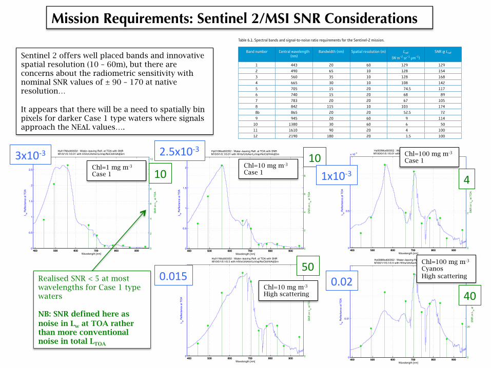
Sentinel 2 offers well placed bands and innovative spatial resolution (10 – 60m), but there are concerns about the radiometric sensitivity with nominal SNR values of ± 90 – 170 at native resolution… It appears that there will be a need to spatially bin pixels for darker Case 1 type waters where signals approach the NEΔL values….

Sentinel-2 Image Quality

39

6. Sentinel-2 Image Quality

The Sentinel-! products will take advantage of the stringent radiometric and geometric image quality requirements. These requirements constrain the stability of the platform and the instrument, the ground processing and the in-orbit calibration. Table ".# shows the spectral band characteristics and the required signal-to-noise ratios for the reference radiances (Lref) defined for the mission. An accurate knowledge of the band equivalent wavelength is very important as an error of # nm can induce errors of several percent on the reflectance, especially in the blue part (atmospheric scattering) and the near-infrared part of the spectrum (vegetation red edge). The equivalent wavelength therefore needs to be known with an uncertainty below # nm.

Obtaining a physical value (radiance or reflectance) from the numerical output provided by the instrument requires knowledge of the instrument sensitivity. Any error on the absolute calibration measurement will directly a$ect the accuracy of this physical value. This is why a maximum %% absolute calibration knowledge uncertainty was required for the mission, with an objective of &%. In the same way, the cross-band and multitemporal calibration knowledge accuracies were set to &% as an objective and #%, respectively. Moreover, the nonlinearity of the instrument response will be known with an accuracy of better than #% and will have to be stable enough that the detector non-uniformity can be calibrated at two radiance levels in flight.

The system MTF is specified to be higher than '.#% and lower than '.& at the Nyquist frequency for the #' m and !' m bands, and lower than '.(% for the "')m bands.

The geometric image quality requirements are summarised in Table) ".!. The accuracy of the image location, !' m without ground control points (GCPs), is very good with regard to the pixel size and should be su*cient for most applications. However, from the Level-# processing description, most of the Sentinel-! images will benefit from GCPs and will satisfy the #!.%)m maximum geolocation accuracy.

The main instrument performance specifications are recalled in Table)".&, with an example representing the spectral performance measured using the EM filter programme shown in Fig.) ".#, and the MultiSpectral Instrument spectral requirements in Table)".(.

Band number Central wavelength (nm)

Bandwidth (nm) Spatial resolution (m) Lref

(W m!2"sr!1"µm!1)

SNR @ Lref

1 443 20 60 129 1292 490 65 10 128 1543 560 35 10 128 1684 665 30 10 108 1425 705 15 20 74.5 1176 740 15 20 68 897 783 20 20 67 1058 842 115 10 103 1748b 865 20 20 52.5 729 945 20 60 9 114

10 1380 30 60 6 5011 1610 90 20 4 10012 2190 180 20 1.5 100

Table 6.1. Spectral bands and signal-to-noise ratio requirements for the Sentinel-2 mission.

Realised SNR < 5 at most wavelengths for Case 1 type waters NB: SNR defined here as noise in Lw at TOA rather than more conventional noise in total LTOA

10 10 3x10-‐3 2.5x10-‐3 3x10-‐3

1x10-‐3

0.015 0.02

4

40

50

Mission Requirements: Sentinel 2/MSI SNR Considerations

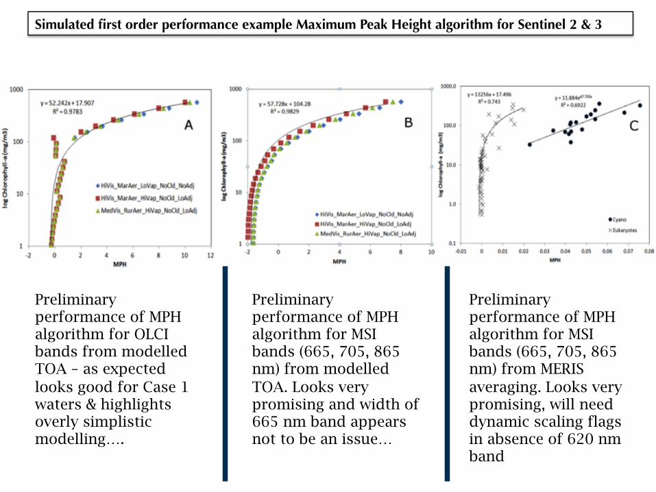
Preliminary performance of MPH algorithm for OLCI bands from modelled TOA – as expected looks good for Case 1 waters & highlights overly simplistic modelling….

Preliminary performance of MPH algorithm for MSI bands (665, 705, 865 nm) from modelled TOA. Looks very promising and width of 665 nm band appears not to be an issue…

Preliminary performance of MPH algorithm for MSI bands (665, 705, 865 nm) from MERIS averaging. Looks very promising, will need dynamic scaling flags in absence of 620 nm band

Simulated first order performance example Maximum Peak Height algorithm for Sentinel 2 & 3

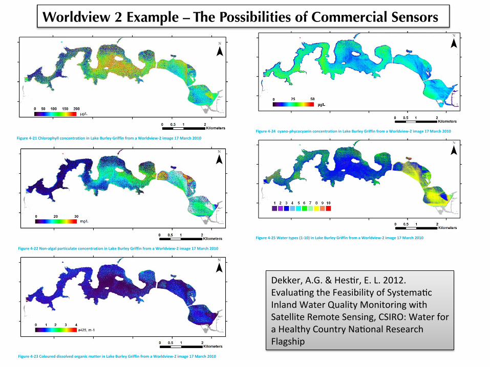
Dekker, A.G. & HesAr, E. L. 2012. EvaluaAng the Feasibility of SystemaAc Inland Water Quality Monitoring with Satellite Remote Sensing, CSIRO: Water for a Healthy Country NaAonal Research Flagship

Worldview 2 Example – The Possibilities of Commercial Sensors

!" # $%&'(&)*+, )-. /.&0*1*'*)2 34 520).6&)*7 8+'&+9 :&).; <(&'*)2 =3+*)3;*+, >*)- 5&).''*). ?.63). 5.+0*+,

@58?A B&+9 C :&).; !" #!$%6.&0(;.6.+)0D )-. EFG? 73;;.7).9 &B=8 H;37.00.9 B&+90&) 9&)& &+9 )-. 7:A=FGI 7 &+9 )-. &B=8 H;37.00.9 :3;'9%*.> J 9&)&K

!"#$%& ' () *+%,-."&/ ( "01#& +2 314& 5$%,&6 7%"22"8 9: ;1%<= ()9)

/*,(;. L JM 0-3>0 & :3;'9N*.> J )>3 6.).; 0H&)*&' ;.03'()*3+ *6&,. 34 B&O. F(;'.2 P;*44*+ 3+ QR =&;7-JMQMK /*,(;. L JQD /*,(;. L JJ &+9 /*,(;. L JS 0-3> )-. ;.0(')0 34 &HH'2*+, )-. &B=8 &',3;*)-6 )3 )-*0*6&,. H;39(7*+, 6&H0 34 @TBD EGU &+9 @VA=K 536. 0.+03; +3*0. &+9 0);*H*+, *+9*7&)*%. 34 )-. ;.'&)*%.'2'3> ;&9*36.);*7 ;.03'()*3+ *0 %*0*1'. *+ )-.0. *6&,.0K

!"#$%& ' (9 >=,+%+?=6,, <+8<&8@%1@"+8 "8 314& 5$%,&6 7%"22"8 2%+0 1 *+%,-."&/ ( "01#& 9: ;1%<= ()9)

!"#$%#&'() &*+ ,+#-'.'$'&/ 01 2/-&+3#&'4 5($#(6 7#&+8 9%#$'&/ :0('&08'() ;'&* 2#&+$$'&+ <+30&+ 2+(-'() = >?

!"#$%& ' (( )*+ ,-#,- .,%/"0$-,/& 0*+0&+/%,/"*+ "+ 1,2& 3$%-&4 5%"66"+ 6%*7 , 8*%-9:"&; ( "7,#& <= >,%0? (@<@

!"#$%& ' (A B*-*$%&9 9"CC*-:&9 *%#,+"0 7,//&% "+ 1,2& 3$%-&4 5%"66"+ 6%*7 , 8*%-9:"&; ( "7,#& <= >,%0? (@<@

,')%8+ @ A@ -*0;- &*+ 8+-%$& 01 #BB$/'() # -+3' +3B'8'4#$ .$%+ )8++( #$)#$ B')3+(& C4/#(0 B*/404/#('(D#$)08'&*3 &0 &*+ 708$6E'+; A '3#)+F ,')%8+ @ A> -*0;- &*+ 6'-&8'.%&'0( 01 &*+ ;#&+8 &/B+- C3+#-%8+66%8'() &;0 1'+$6 4#3B#')(- '( G#(%#8/ #(6 :#84* AHIHD #44086'() &0 &*+ #J:5 #$)08'&*3 B804+--'()F K*+#$)08'&*3 6+&+83'(+- 108 +#4* B'L+$ '( +#4* '3#)+ ;*#& &*+ .'0 0B&'4#$ B80B+8&'+- #8+ C1803 ;*'4* -B+4'1'4!" #!$% -#3B$+ (%3.+8+6 I &*80%)* &0 IHM -++ J+)+(6DF 5( &*+ '3#)+M &*'- 6'-&8'.%&'0( -*0;- B#&&+8(- ;*'4*$'N+$/ '(6'4#&+ &*+ ;#&+8 3#--+- 603'(#(&$/ B8+-+(&F

K*%- &*+ #J:5 #$)08'&*3 4#( #$-0 B80"'6+ '3#)+- 01 ;#&+8 &/B+- #(6 *0; &*+/ #8+ 6'-&8'.%&+6 6%+ &0.'0$0)'4#$M 4*+3'4#$ #(6 B*/-'4#$ 6'11+8+(4+-F

!" # $%&'(&)*+, )-. /.&0*1*'*)2 34 520).6&)*7 8+'&+9 :&).; <(&'*)2 =3+*)3;*+, >*)- 5&).''*). ?.63). 5.+0*+,

!"#$%& ' (' )*+,- ./*)-)*+,", )-,)&,0%+0"-, ", 1+2& 3$%4&* 5%"66", 6%-7 + 8-%49:"&; ( "7+#& <= >+%)/ (?<?

!"#$%& ' (@ 8+0&% 0*.&A B< <?C ", 1+2& 3$%4&* 5%"66", 6%-7 + 8-%49:"&; ( "7+#& <= >+%)/ (?<?

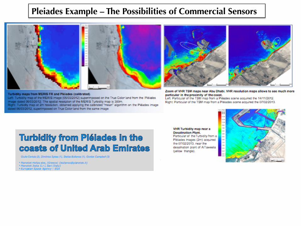
Pleiades Example – The Possibilities of Commercial Sensors

Summary: •  Landsat 8 offers high quality radiometry at 30 m resolution, community processing

tools, and demonstration of validated products for Chl a, TSS, CDOM and cyanobacteria. Revisit time may present problems for operational/ecological applications, and limited spectral resolution may hamper constituent disambiguation across wide ranges of water types.

•  Sentinel 2 will offer good spectral coverage, and 5 day revisit time in full constellation but is likely to require spatial binning to 60m to offer sufficient SNR for aquatic applications. Range of products such as Chl a, TSS, CDOM and cyanobacteria across wide range of water types should be feasible with appropriate AC, SNR etc evaluation. Community processing tools required.

•  Emerging AC tools such as SeaDAS modules and ACOLITE are vital components and Sentinel 2 options need to be demonstrated….

•  Demonstrated ability to exploit commercial sensors such as WV-2 & 3, Pleiades, RapidEye but likely to be exploited on specific case basis….

What new processes and features can be detected in ports, estuaries and inland waters?

Documents

Stewart Bernard (CSIRO)