Stewart Platform Actuator for

Direct Access Cochlear Implant

A thesis submitted to the

Graduate School

of the University of Cincinnati

in partial fulfillment of the

requirements for the degree of

MASTER OF SCIENCE

in the department of Mechanical Engineering

of the College of Engineering and Applied Sciences

by

Gaurav Patil

Bachelor of Engineering

Shivaji University, Kolhapur

2011

Thesis Committee Chair: Vasile Nistor, PhD

Defense Committee Chair: David Thompson, PhD

ABSTRACT

This thesis is focused on devising a setup to perform a posterior tympanotomy part of the

Cochlear Implant Surgery using a Stewart Platform Actuator, which is a six degrees-of-freedom

robot, with six linear actuators. The work described in this thesis covers (1) redesign of the

actuator, (2) algorithm for its operation based on the inverse kinematics of the Stewart Platform,

(3) surgical path planning based on conversion of CT-scan images into 3D models (4)

registration of the actuator position using anchor screws and (5) a non-invasive registration

technique for the actuator using 3D laser scanning technique.

Cochlear implantation surgery requires the surgeon to drill through the temporal bone and

end by opening up at the basal turn of the cochlear tissue. The surgeon has to excavate through a

large volume of bone to identify and avoid the important anatomical structures. We are going to

prototype a robotic device to aid in the process in order to increase the accuracy while

minimizing the risk to patients. This robot is different from others in that it is designed

specifically for cochlear implantation surgery and other surgeries requiring drilling through the

temporal bone, which will optimize the device’s effectiveness and minimize the cost.

The actuator that we have developed is based on the concept of Stewart Platform robot

which has a bottom platform with six spherical joints attached to six linear actuators which then

connect to spherical joints to support a top plate. The top plate is attached to a surgical drill

which protrudes downward through the center of the bottom hole of the platform. The plan is to

fix the bottom platform on the top of the patient’s head and then feed the path to the robot for

drilling the hole. The challenge here is to find a straight non-collision path (Direct access

Cochlear Implant) from the surface of the mastoid to the basal turn of the cochlea. This path will

be determined by using the CT-scan images of the patient’s skull which will then be converted

into 3D models using a software called Amira.

The next important part of this project includes accurate positioning of the robot’s bottom

plate on top of the patient’s head. In the first approach discussed by this thesis, the plan is to fix 3

or more anchor screws into the patient’s skull before collecting the CT-scan images. Then a

personalized 3D printed fixture will be designed, using the 3D models from Amira, which will

then attach to the bottom of the plate and also screw on to the anchor screws. In the second

approach we have set the groundwork to make the positioning non-invasive with the use of 3D-

laser scanning technology and eliminating the anchor screws.

Initial tests show feasibility of this kind of procedure and further improvements can lead

to a foolproof system for Cochlear Implantation surgery. The future work for this project

includes making this robot semi-automatic with the use of haptic feedback. The non-invasive

registration processes will also be explored in depth.

ACKNOWLEDGEMENTS

I’d like to express my special appreciation and thanks to my thesis and research advisor

Dr. Vasile Nistor, without whose support this work would have been impossible. I’d like to thank

him for encouraging my research and providing enough freedom for the tasks I have undertaken

towards this thesis. I’m so glad that I get to work with him towards my PhD.

I’d also like to thank Professor Daniel Humpert, who has been a great mentor for me

during my time at the University of Cincinnati and has played a very important role in my

development here. I’d also like to thank Dr. Debi Sampsel from the College of Nursing for all

the inspiration throughout the past couple of years. Dr. Sampsel and Professor Humpert are the

collaboration due to which my interest towards healthcare related engineering has grown over

time.

I’d also like to thank Dr. David Thompson for his guidance throughout my time at the

University of Cincinnati and making it smoother for me to work in the Biomedical Engineering

Department towards my thesis. I’d also like to thank Dr. Manish Kumar for agreeing to be on my

committee and I’m looking forward to his inputs towards our research after he returns to the

University of Cincinnati. I’d also like to thank Dr. Grant Schaffner for his inputs to our research

from time to time and I’m glad to have him on my thesis committee too.

I’d also like to thank David Cowens and Dr. Ravi Samy for setting up the groundwork for

this project. I’d also like to thank all the professors at UC, whose courses I took and the

knowledge earned from them some way or the other was applied towards this research.

Lastly, I’d like to thank my family and friends without whom I can’t even imagine

getting where I’m right now.

Table of Contents

Chapter 1. Background and Introduction ........................................................................................ 1

1.1 What is a cochlear implant? .................................................................................................. 1

1.2 Related Anatomy .................................................................................................................. 1

1.3 Steps involved in the surgical procedure .............................................................................. 3

1.4 Statistics and complications involved ................................................................................... 6

1.5 Need of a surgical actuator for CI surgery ............................................................................ 8

1.6 Hypothesis............................................................................................................................. 9

1.7 Significance of our work ....................................................................................................... 9

1.8 Outline of this thesis ........................................................................................................... 10

Chapter 2. Literature Review ........................................................................................................ 11

2.1 Minimally invasive CI surgery ........................................................................................... 11

2.2 Use of Robotic systems for CI ............................................................................................ 11

Chapter 3. Methodology ............................................................................................................... 15

3.1 Converting CT-scan images to 3D models and path planning for Direct Access CI ......... 15

3.2 The Stewart Platform Actuator ........................................................................................... 16

3.3 Minimally invasive registration with Anchor screws ......................................................... 20

3.4 Non-invasive registration of the Stewart Platform Robot................................................... 21

Chapter 4. Implementation............................................................................................................ 23

4.1 Planning the straight line path............................................................................................. 23

4.1.1 Fixing anchor screws ................................................................................................... 23

4.1.2 Acquiring CT-scan images .......................................................................................... 24

4.1.3 Identifying the significant anatomical structures ......................................................... 24

4.1.4 Segmenting the images and creating 3D models ......................................................... 27

4.1.5 Path planning ............................................................................................................... 28

4.2 Stewart platform actuator .................................................................................................... 30

4.2.1 Construction of the Stewart Platform Actuator ........................................................... 30

4.2.2 Algorithm for the Stewart Platform actuator ............................................................... 33

4.2.3 Commands for motor control ....................................................................................... 36

4.3 Non-invasive registration .................................................................................................... 37

4.3.1 Laser Scanning and Image acquisition ........................................................................ 37

4.3.2 Calibration.................................................................................................................... 38

4.3.3 Point cloud creation from the captured image sequence ............................................. 43

4.3.4 Registration of the Point Cloud.................................................................................... 45

Chapter 5. Tests and Results ......................................................................................................... 47

5.1 Test for the accuracy of the Stewart Platform Actuator ..................................................... 47

5.1.1 Test setup ..................................................................................................................... 47

5.1.2 Test for Angular Accuracy........................................................................................... 48

5.1.3 Test for Positional Accuracy ........................................................................................ 49

5.2 Test for the accuracy of laser scanning and registration ..................................................... 51

5.3 Test for registration of points tracked by the tool tip .......................................................... 55

Chapter 6. Conclusion and Future Work ...................................................................................... 58

Chapter 7. References ................................................................................................................... 60

List of Figures

Figure 1. Anatomy of the ear .......................................................................................................... 2

Figure 2. Anatomy of the ear with a CI .......................................................................................... 3

Figure 3. Planning the surgery ........................................................................................................ 4

Figure 4. Cutting the skin open and exposing the mastoid bone .................................................... 5

Figure 5. Creating an incision for the receiver ............................................................................... 5

Figure 6. Cochleostomy and electrode insertion............................................................................. 6

Figure 7. Fixing everything in place ............................................................................................... 6

Figure 8. Worldwide statistics for total number of CI .................................................................... 7

Figure 9. Solidworks model of the Stewart Platform Robot ......................................................... 17

Figure 10. Co-ordinate axes at the reference point and start and end points of the path .............. 19

Figure 11. Registration using anchor screws ................................................................................ 21

Figure 12. Setup for the Non-invasive Registration of the Stewart Platform Actuator ................ 22

Figure 13. Steps involved in the Registration Technique ............................................................. 22

Figure 14. M2.5 Anchor screws .................................................................................................... 23

Figure 15. Visualization of CT-scan data in Amira ...................................................................... 24

Figure 16. Identifying the turns of cochlea ................................................................................... 25

Figure 17. Identifying cochlea from a different view ................................................................... 25

Figure 18. Identifying the facial nerve .......................................................................................... 26

Figure 19. Identifying the vestibular system................................................................................. 26

Figure 20. Segmentation in Amira ................................................................................................ 27

Figure 21. 3D models from segmented data ................................................................................. 28

Figure 22. Planned straight path in Siemens NX .......................................................................... 29

Figure 23. Planned straight path in Siemens NX .......................................................................... 30

Figure 24. Initial design and build for the Stewart Platform Actuator ......................................... 31

Figure 25. Revised design for the Stewart Platform Actuator ...................................................... 32

Figure 26. Revised build of the Stewart Platform Actuator.......................................................... 32

Figure 27. Path to be followed by the tool tip............................................................................... 34

Figure 28. (a) Line Laser Pointer (b) Line Generated on an Object ............................................. 37

Figure 29. Schematic Layout of the Registration Procedure ........................................................ 38

Figure 30. (a) 6cm x 6cm grid used for calibration (b) Image of the grid captured by the camera

....................................................................................................................................................... 39

Figure 31. (a) Binary Image of the grid (b) Plot for the Hough lines ........................................... 41

Figure 32. Calibration image for 10 mm height at nth laser line position ..................................... 42

Figure 33. Cropped sample Image from the Image sequence ....................................................... 44

Figure 34. Test setup ..................................................................................................................... 47

Figure 35. Results for the Angular Accuracy test (0 and 5 degrees) ............................................ 48

Figure 36. Plan for the Positional Accuracy Test ......................................................................... 49

Figure 37. Results for the Positional Accuracy Test..................................................................... 49

Figure 38. Different Positions for the test object (1)Default position [0°] (2) Position 2 [90°] (3)

Position 3 [45°] ............................................................................................................................. 51

Figure 39. Different Positions for the test object (4) Position 4 [135°] (5) Position 5 [180°] (6)

Position 5 [30°] (7) Position 5 [60°] ............................................................................................. 52

Figure 40. ICP cost function vs the Angle of rotation for different positions of the test object ... 54

Figure 41. Four input points on the test object ............................................................................. 55

Figure 42. Points tracked by the actuator using the registration data from the laser scan for 45°

rotation .......................................................................................................................................... 56

Figure 43. Points tracked by the actuator using the registration data from the laser scan for 90°

rotation .......................................................................................................................................... 56

Figure 44. Points tracked by the actuator using the registration data from the laser scan for 135°

rotation .......................................................................................................................................... 57

Figure 45. Points tracked by the actuator using the registration data from the laser scan for 180°

rotation .......................................................................................................................................... 57

List of Tables

Table 1. Comparison between techniques used by different researchers ..................................... 14

Table 2. Positional Errors ............................................................................................................. 50

Table 3. Estimated angles of rotation from the registration data .................................................. 53

1

Chapter 1. Background and Introduction

1.1 What is a cochlear implant?

According to National Institute of Deafness and other Communication Disorders [1], a

cochlear implant(CI) is a surgical procedure where a small, complex electronic device is fitted

into the patient’s skull to provide a sense of sound to a person who is profoundly deaf or severely

hard-of-hearing. An electrode is inserted and permanently fixed into the patient’s cochlear nerve

which lets the signals generated by cochlear implant to be transferred, by the way of cochlear

nerve, to the brain and recognized as sound. The electronic device consists of three parts: (1) a

speech processor, (2) a transmitter-receiver pair and (3) an electrode array.

A speech processor, which sits behind the ear like a common hearing aid, picks up sound

from the environment using a microphone and converts it into a signal that can be

transmitted using an electrode to the cochlear nerve.

A transmitter sits outside the skin and is magnetically attached to a receiver which is

surgically embedded inside the skin. This pair enables the signals from the processor to be

converted into electric impulses.

An electrode array, which coils into the cochlear nerve, is a group of electrodes that

transfers the impulses from the receiver to stimulate different parts of the cochlear nerve.

1.2 Related Anatomy

Figure 1 shows the anatomy of the ear, which shows the external, middle and inner

portions of the ear. The outer ear is made of ridged cartilage covered by skin and is called the

pinna. A small canal starting from the external ear carries the sound waves to the ear drum also

called the tympanic membrane. Sound causes the tympanic membrane and the attached tiny

2

bones to vibrate and these vibrations are conducted to the cochlea. The cochlea is a spiral shaped

nerve in the inner ear, which transforms sound into nerve impulses. The semi-circular canals are

fluid filled and used to notify the balance and the head position to the bone. The Eustachian tube

drains fluid from the middle ear into the pharynx. Figure 2 shows the anatomy of the ear with a

CI.

Figure 1. Anatomy of the ear

3

Figure 2. Anatomy of the ear with a CI

1.3 Steps involved in the surgical procedure

Before the actual surgery, a patient goes through different audiology tests and CT scan

evaluations and then a specialist surgeon decides if the patient is a suitable candidate for a CI.

After the approval of the CI surgery by FDA in 1985, many methods have been proposed by

researchers all over the world in order to reduce the risks involved. The most commonly adapted

surgical technique [2] introduced by Clark et al. goes through the following basic steps

1) A small area of the scalp directly behind the ear is shaved and cleaned as shown in Figure 3.

2) A cut is made behind the ear and the skin over the mastoid is opened to create a flap as

shown in Figure 4.

3) Mastoidectomy is done to create a pocket for the receiver as shown in Figure 5.

4

4) Posterior Tympanotomy is done, to make a passage for insertion of the electrode, which

opens into the round window niche.

5) Cochleostomy is done so that the electrode can be inserted into the cochlear tissue which

uses the cochlear tissue as a guide to curl as shown in Figure 6.

6) The electrode is inserted into the scala tympany and the maximum possible insertion is

achieved (100% in most cases).

7) Electrode and receiver is connected and fixed in place before closing the skin and applying

dressing.

Figure 3. Planning the surgery

5

Figure 4. Cutting the skin open and exposing the mastoid bone

Figure 5. Creating an incision for the receiver

6

Figure 6. Cochleostomy and electrode insertion

Figure 7. Fixing everything in place

1.4 Statistics and complications involved

According to the Hearing Loss Association of America [3], as of December 2012,

approximately 324,200 people worldwide have received implants, which rose from 150,000 in

2008 and 188,000 in 2010. In the United States, roughly 58,000 adults and 38,000 children have

7

received them, as of December 2012. According to hearing loss statistics from Cochlear Implant

Online [4], there are 36 million Americans who have hearing loss and this number is predicted to

double by 2030 as baby boomers are reaching their retirement age. Currently, only one out of

five people who can benefit from hearing aid uses one and only 7% of people who are qualified

for CI actually have one. All these figures show that the number of people getting a CI is going

to rise extensively in the coming years.

Figure 8. Worldwide statistics for total number of CI

Though CI surgeries have been practiced and mastered for more than fifty years, the

traditional surgical method still has some temporary and permanent complications associated

with it. Risks of permanent complications include the damage to important anatomical structure

which includes the facial nerve, chorda tympani nerve, vestibular system, sigmoid sinus, carotid

artery and labyrinth during posterior tympanotomy. Also, the pointed end of the electrode can

puncture through the cochlear tissue while insertion. Facial nerve damage can lead to permanent

paralysis of the face and chorda tympani damage can lead to permanent loss in the ability to

taste. Damage to the vestibular system can lead to imbalance and difficulty with co-ordination.

Though carotid artery is not within the surgical approach, it is the main blood supply artery to the

0

50,000

100,000

150,000

200,000

250,000

300,000

350,000

2008 2010 2012

Total number of Cochlear Implants

worldwide

8

brain and damage to it can be fatal. Also, inexperienced surgeons can exert uneven forces on the

electrode, while insertion, resulting in the bucking of the electrode itself.

Takeshi Kubo, MD et al. [5] have identified temporary complications and classified them

as minor and major complications from the data they collected from major Cochlear Implant

centers. According to their analysis, minor complications include tinnitus (75% of cases),

dizziness or vomiting (38% of cases), taste disturbance (22% of cases), infection (8% of cases)

and facial palsy (2% of cases). Most of these complications occur immediately after the surgery

and tend to disappear over time. Major complications include facial nerve stimulation (14% of

cases), poor response of auditory nerve (2.5% of cases), electrode exclusion (2.2% of cases),

device migration (1.85% of cases), electrode misplacement (1.3% of cases) and device failure

(2.1% of cases). Most of these complications can be resolved by a revision surgery.

1.5 Need of a surgical actuator for CI surgery

It has already been established that the number of CI surgeries being performed

worldwide is rising and will keep on rising in the future. Several factors could affect the large

scale adoption of CI viz. lack of specialists, risks associated with current technique, costs, etc.

There is a scarcity of specialist surgeons who can perform CI surgery in most of the developing

nations. Also, most of the permanent risks involved during the surgery are involved during

posterior tympanotomy. These risks include damage to important anatomical structures due to

lack of vision control during drilling. To avoid this surgeon has to drill through a lot of bone

material and identify the tissue structure before completing the passage to round window niche.

All this contributes in making this surgery expensive and complicated. All of this can be avoided

by using a robot to perform the surgery on a pre-planned path. The path for the robot can be

planned using µCT scan images with the help of a specialist and can be fed to the robot to

9

perform the surgery. Real-time monitoring of the robot by a specialist will make this kind of

surgery safe for common practice.

1.6 Hypothesis

Our first hypothesis is that, a straight non-collision path can be determined from the

surface of the mastoid bone to the basal turn of the cochlea from CT-scan images using Amira,

commercial software already available in our lab.

Our second hypothesis is that, the Stewart platform actuator developed in our lab has the

required accuracy and precision to drill on the straight path planned from the CT-scan images.

Anchor screws and 3D printed plastic fixture can be used for the registration of the CT-scan

images to the axes of the actuator.

Our third hypothesis is that, after achieving the required accuracy for the Stewart

Platform actuator, a non-invasive registration technique can be developed, with the use of 3D

laser scanning, to eliminate the use of anchor screws.

1.7 Significance of our work

Our work addresses the issue of reducing risks during the posterior tympanotomy part of

the CI surgery and increasing its efficiency with the use of robotic actuator. Many attempts have

been [6]–[8] and are being made to develop a surgical system working with a robot to perform

CI surgeries. Most of these methods incorporate industrial robots to drive the surgical tool. All of

these methods make use of very expensive optical tracking and positioning systems for the robot.

For our system, we want to build a robot specific for this kind of surgery, which will be based on

the concept of a six link Stewart Platform Robot. Also, we want to achieve the required accuracy

and precision for the actuator while positioning it minimally invasive and taking it a step further

10

to make it non-invasive. We also want to explore simpler methods to incorporate a surgeon

control over the robot making it a semi-autonomous system with the use of haptic feedback

devices.

1.8 Outline of this thesis

The work covered in this thesis is based on initial work by David Cowens, an

undergraduate student in Biomedical Engineering. This initial effort covered a prototype design

and build for the Stewart Platform Actuator. The work described in this thesis covers the (1)

redesign of the actuator, (2) an algorithm for its operation based on the inverse kinematics of the

Stewart Platform, (3) surgical path planning based on conversion of CT-scan images into 3D

models (4) new concept of registration of the actuator position using anchor screws and (5) a

non-invasive registration technique for the actuator using 3D laser scanning technique.

So far in Chapter 1, the steps involved in CI surgery and the importance of our work have

been discussed. Chapter 2 discusses some of the relevant work done by other researchers. The

methodology that we used for our work is explained in Chapter 3. Chapter 4 discusses

implementation of the path planning from 3D models created using CT-scan images, the

algorithm to operate the Stewart Platform actuator and the laser scanning procedure to create the

point cloud data and its registration. Chapter 5 discusses some initial tests carried out on faux

bone sheets to test the accuracy of the actuator and the tests for the feasibility of the laser

scanning registration and the results obtained. Chapter 6 summarizes the conclusions obtained

from the results in chapter 5 and discusses potential avenues for improvement and additional

research in this area.

11

Chapter 2. Literature Review

2.1 Minimally invasive CI surgery

The steps involved in the traditional and most widely used surgical procedure for CI

surgery [2] introduced by Clark et al. have already been explained in Chapter 1. The risks and

drawbacks of this method have also been discussed. To avoid most of the risks, many researchers

have come up with methods that can lead to a better surgery and can be minimally invasive.

These methods can also make the CI surgery simpler and feasible by using a robotic system. One

of such methods, called the Percutaneous Cochlear access method [9], was introduced by

Labadie et al. This method uses CT-scan images to perform pre-operative planning. Before

taking CT-scan images 3 incisions are made in patient’s skin and self-tapping anchors are

screwed into the skull surrounding the temporal bone. These anchors are later used as reference

points for planning the surgery and also to position the guide for the drill. These CT-scan images

are used to segment all the anatomical structures which in turn are used to find a no-collision

straight path that bypasses all critical anatomical features at a safe distance. This path is

calculated from the entry point, anywhere on the bone surface between the anchors, to the end

point, the basal turn on the cochlea. Using this path and anchors as indexing reference a drill

guide is prototyped specifically for that patient. During surgery, the drill guide is screwed to the

anchors and this arrangement governs the path of the drill all the way to the cochlea.

This paper shows that a straight path can be planned for a CI surgery and the use of CT-

scan images for pre-operative planning can lead to the most minimally invasive CI surgery.

2.2 Use of Robotic systems for CI

12

While looking at the use of robotic systems for CI surgery, the focus was on two things-

(1) surgery path planning technique and (2) the robot positioning and tracking technique or the

registration technique.

Labadie et al. have used an Image guided robot [8] for demonstrating the procedure

termed by them as Percutaneous Cochlear access. Their path planning technique has already

been discussed in the previous point. For registration of radiographic images to the patient they

used fiducial markers that can be identified both in radiographs and on the patient. A dental bite

block with fiducial markers on it and a fiducial frame is used while taking the CT-scan images

and also while performing the surgery. The fiducial markers act as reference while planning the

path of the surgery and also for the infrared tracker to register the anatomy of the skull with the

CT scan data. Trackers are also put on the drill so that the drill can be tracked accurately in real-

time with respect to the skull. The advancement of the drill is tracked in real-time and care is

taken to avoid vital structures while performing the drilling operation. Though the type of robot

used for advancing the drill hasn’t been mentioned, this paper explains in detail the positioning

and tracking system used.

Other approach introduced by Majdani et al. [6] uses just the registration markers on the

skull as a reference for planning the surgery and positioning the robot. They have used a surgical

planning software called iPlan[10] to segment the anatomy. Based on this segmentation, a

software which uses pattern search optimization method is used to determine accurate optimal

co-ordinates of the drill trajectory. This paper discusses a rather simple approach for determining

the optimal path from a large set of possible paths by using a min-max rule to exclude some

paths. A Polaris stereo camera is used to register the position of the base of the robot, the drill

attached to it and the surgical specimen, each of which is marked with custom-made reference

13

reflectors. KR3 (KUKA GmbH, Augsburg, Germany) robot is used to drive the drill and is

operated by a custom-made program called ‘Medilab’ based on MATLAB/Simulink. The

important points to be noted from this research were the method to determine the optimal path

and that the average length of drill-travel being 27.09 ± 2.88 mm.

Another attempt to perform robotic CI surgery is discussed by Bell et al. [7]. This

approach uses a five-degree of freedom serial custom-built surgical robot which is light enough

to be mounted on a standard OR table. The robot has a built in force-torque sensor which is used

to provide haptic feedback to the operator controlling the robot from outside the sterile

environment using a touch screen interface. Reference screws are fixed in the skull before

imaging. A cone-beam CT is used to acquire high resolution images which are then segmented

and converted into 3D models using Amira. The path for the surgery is planned manually using

the 3D models. Calibration process is done by using the robot as a registration device by

touching the reference screws with the tip. Once the registration is complete the tip is replaced

with a drill. The drilling is done in two steps- first drilling a starter hole with a short, stiff spiral

drill and then drilling the full-depth tunnel.

The following table gives a short comparison of all the three approaches discussed above.

14

Table 1. Comparison between techniques used by different researchers

Approach Registration Path planning Positioning/tracking

Labadie et al.

Dental bite block

and fiducial frame

Percutaneous Cochlear

access method

Infrared tracking with

trackers on dental bite

block, fiducial frame

and the drill

Majdani et al. Registration markers

Software which uses

pattern search

optimization method is

used to find optimal path

Optical tracking with

reflectors on the base of

the robot, the drill

attached to it and the

surgical specimen

Bell et al. Registration screws

Manual planning using

3D models segmented in

Amira

Touching the tip of the

robot, attached to the

OR table, to the

registration screws

15

Chapter 3. Methodology

3.1 Converting CT-scan images to 3D models and path planning for Direct Access CI

Computed Tomography (CT) [11] is a technology which uses computer controlled X-rays

to produce virtual slices of the scanned object without cutting it open. Each virtual slice is an

image made up of pixels (also called as voxels) whose intensity represents the relative radio-

density. The intensity of pixels representing a bone is higher than the ones representing tissue.

This variation in density can be used to classify or segment the image to identify deferent

anatomical structures. Stacking these images can lead to 3D models of the object which is

scanned; in our case it will be a temporal bone or the structure surrounding the ear.

Several software packages are available for segmenting CT-scan images and converting

them into 3D models. The software available in our research lab was Amira [12] which will be

used for our purpose. Amira is a powerful 3D software platform which lets us visualize and

analyze CT-scan data. The segmentation is done manually and 3D models can be created. The

accuracy of the 3D models depends on the accuracy of the CT-scan data. Various online

resources like the Radiology assistant [13] are available which can be used to identify different

anatomical structures, which can be a tedious job. Amira also has features like ‘interpolate data’,

which can automate the segmentation part to some extent. The procedure followed in Amira will

be discussed, in detail, in the next chapter.

Before taking the CT-scan images anchor screws will be screwed into the specimen,

which can be used as a reference for planning the path and also to register the reference frames

of both the robot and CT-scan images. Once the required 3D models are created, they can be

16

exported to Siemens NX[14] and then a no-collision path can be planned. Some of the conditions

that have to be satisfied by this path are

1) It has to be a straight line

2) The end point should end at the basal turn of the cochlea

3) The start point should be on the surface of the temporal bone right below the skin

4) The path shouldn’t collide with any of the anatomical structures viz facial nerve,

vestibular system and chorda tympani nerve.

After a path satisfying all the above conditions is selected, the co-ordinates of the start

point and the end point with reference to the anchor screws can be determined and they can be

used to operate the actuator.

3.2 The Stewart Platform Actuator

Stewart Platform [15] is a parallel robot which has six linear joints, also called legs,

which act as actuators mounted in pairs to the base, crossing over to three mounting points on the

top plate. Devices attached to the top plate can be moved in six degrees of freedom with respect

to the base frame. The actuator that we have developed is based on the concept of Stewart

Platform robot which has a bottom platform with six spherical joints attached to six linear

actuators. The linear actuators then connect to another six spherical joints to support a top plate.

A surgical drill is attached to the top plate and protrudes downward through the center of the

bottom ring of the platform. All this arrangement is mounted on an aluminum platform which

can be fixed securely over the patient’s head. Figure 9 shows the Solidworks model of the

actuator.

17

For our application we want the Stewart Platform actuator to follow a straight line path,

for which the inverse kinematics of the robot can be simplified and put together in an algorithm.

The inverse kinematics can be used to determine the lengths of each leg at various positions of

the robot and by changing lengths different transformations can be achieved.

Figure 9. Solidworks model of the Stewart Platform Robot

Before writing the code to operate this robot it’s important to understand the inverse

kinematics and to derive the formulae which will be used to write the code. Any position for the

tool tip can be determined by the lengths of all the legs and by changing the lengths of the legs

the tip can be made to follow the desired path. The length of all the legs can be calculated from

the co-ordinates of the joints on the top plate and the co-ordinates of the joints on the bottom

platform. If the reference co-ordinate frame is assumed to be in the plane of the bottom joints and

equidistant from all of them, the relative position of the joints on the top plate will directly

18

determine the position of the tool tip. So, if the transformation matrix for the position of tool tip

is known, the co-ordinates of the joints on the top plate can be determined and they can be used

to calculate the lengths of the legs at that position.

The actuator will be used to drill from point P1 (starting point on the surface of the

temporal bone) and P2 (basal turn of the cochlea) in a straight line. Let O be the origin of the

reference frame which is at the center of the base plate. When the length of all legs is at

minimum, the tool tip will be at point P. The co-ordinates of the top plate can be calculated from

the co-ordinates of the tool tip as they are rigidly linked. The co-ordinates of points P1 and P2

with respect to O will be determined from the 3D model of the patient’s skull. Figure 10 shows

the co-ordinate frames at the reference point O and start and end points P1 and P2. Line P1P2 is

the straight path on which the drill has to follow.

Let (x1, y1, z1) be the co-ordinates of point P1 and (x2, y2, z2) be the co-ordinates of point

P2 with respect to reference frame O. Vector P1P2 can be used to calculate the roll, pitch and yaw

for the tool tip at points P1 and P2 as shown in figure x

Roll, γ = tan-1 (𝑦1− 𝑦2

𝑧1− 𝑧2)

Pitch, β = tan-1 (𝑥1− 𝑥2

𝑧1− 𝑧2) equation (1)

Yaw, α = 0 since the tool tip and in turn the top platform doesn’t rotate in the plane

perpendicular to the Z-axis. Also, all the above angles will be equal for both P1 and P2 as the tool

doesn’t change its orientation between these points.

Roll, pitch, yaw and the co-ordinates of points P1 and P2 can be used to calculate the

transformation matrices for the respective points as follows [16].

19

Figure 10. Co-ordinate axes at the reference point and start and end points of the path

T1 =

[

cos(β)cos (α) sin(γ) sin(β) cos(α) − cos(γ) sin(α) cos(γ) sin(β) cos(α) + sin(γ) sin(α) 𝑥1

cos(β) sin (α) sin(γ) sin(β) sin(α) + cos(α) cos(γ) cos(γ) sin(β) sin(α) − sin(γ) cos(α) 𝑦1

−sin (β) sin(γ) cos(β) cos(γ) cos(β) 𝑧1

0 0 0 1

]

Since α = 0,

T1 = [

cos(β) sin(γ) sin(β) cos(γ) sin(β) 𝑥1

0 cos(γ) − sin(γ) 𝑦1

−sin (β) sin(γ) cos(β) cos(γ) cos(β) 𝑧1

0 0 0 1

] equation (2)

Similarly,

T2 = [

cos(β) sin(γ) sin(β) cos(γ) sin(β) 𝑥2

0 cos(γ) − sin(γ) 𝑦2

−sin (β) sin(γ) cos(β) cos(γ) cos(β) 𝑧2

0 0 0 1

] equation (3)

20

These transformation matrices can be used to calculate the co-ordinates of the top plate

joints for the respective positions of the tool tip. If the vector for the top joint of the ith leg, in the

co-ordinate frame with the origin at tool tip P, is assumed to be 𝐴𝑖𝑃= [xai yai zai 1]T, the

homogenous co-ordinate for the ith joint in the reference frame O, when the tool tip is at point P1

can be calculated by taking the dot product with the Transformation matrix.

𝐴𝑖𝑂= T1 . 𝐴𝑖

𝑃 When tool tip P is at point P1 and similarly

𝐴𝑖𝑂= T2 . 𝐴𝑖

𝑃 When tool tip P is at point P2 equation (4)

For a given position, once the co-ordinates of the joints on top and bottom plates are

known the lengths of the legs can be calculated by simple two-point distance formula. If the co-

ordinates of top and base joints of the ith leg are Ai = [xai yai zai]T and Bi = [xbi ybi zbi]

T

respectively, then the length can be calculated by

li = √(𝑥𝑎𝑖 − 𝑥𝑏𝑖)2 + (𝑦𝑎𝑖 − 𝑦𝑏𝑖)

2 + (𝑧𝑎𝑖 − 𝑧𝑏𝑖)2 equation (5)

These lengths can be used to increase or decrease the actuation of the linear motor

operating on every leg and to achieve the desired tool-tip position.

3.3 Minimally invasive registration with Anchor screws

To fix the platform to patient’s skull the plan is to make use of 3D printer technology

which will help us print patient specific 3D printed fixtures which will attach on one side to the

robot’s platform and on the other side to the anchor screws fixed into the patient’s skull. Also,

from the 3D models a collision free straight line path can be planned for the robot to operate on.

This path will be fed into the robot using an algorithm, written in MATLAB, thus creating a

straight channel for the electrode to be inserted into the cochlea.

21

Figure 11 shows a schematic diagram of the robot attached to the patients head with the

use of anchor screws.

Figure 11. Registration using anchor screws

3.4 Non-invasive registration of the Stewart Platform Robot

In the previous method, for positioning the Stewart Platform actuator the use of anchor

screws is proposed. That technique has the pros of higher accuracy but it can lack the practicality

when the patient needs to have anchor screws in the temporal bone before going in for the CT-

scan and then wait until the surgery is done to get them removed. Eliminating the anchor screws

completely and having the platform positioned non-invasively is thus a better option if the same

accuracy can be achieved. The Non-invasive technique that will be discussed here makes use of

3D laser scanning method. Figure 12 shows the experimental setup for the testing of the non-

invasive registration technique.

22

The steps involved in this technique are 1) Laser scanning and image acquisition 2)

Calibration of the transformation between image and robot axes 3) Creation of the point cloud

from the images captured 4) Registration of the point cloud. These steps and their

implementation will be explained in more detailed in the next chapter.

Figure 12. Setup for the Non-invasive Registration of the Stewart Platform Actuator

Figure 13. Steps involved in the Registration Technique

23

Chapter 4. Implementation

4.1 Planning the straight line path

These are the steps that are required to plan a straight line path from the CT-scan data.

4.1.1 Fixing anchor screws

Figure 14 shows the anchor screws that are chosen for the registration of CT-scan images

with the co-ordinate frame of the Stewart Platform actuator. Three anchor screws will be

screwed into the temporal bone before taking the CT-scan images. These anchor screws are

made of Zinc-plated brass.

While using Zinc-plated brass screws, the scattering of X-rays and the related noise

introduced in the CT-scan images will have to be given a good consideration. Also, obtaining

CT-scan data with these screws will introduce a pre-operative procedure on the patient’s skull

which is not the most feasible option. In spite of these problems, the use of anchor screws is a

preliminary step in solving the bigger problem. Alternate way for registering the CT-scan images

and positioning of the actuator need to be researched and one such non-invasive technique will

be discussed further in this thesis.

Figure 14. M2.5 Anchor screws

24

4.1.2 Acquiring CT-scan images

The most common file format for CT-scan data is ‘.dicom’. DICOM data can be directly

opened and visualized in Amira[12]. The ‘Segmentation Editor’ feature can be used to visualize

the data from all three 2D perspectives and also a combination of all three in a 3D perspective as

shown in Figure 15. The resolution of the CT-scan data determines the overall accuracy of the

visualization, segmentation and the path planning. But if the resolution is too high it also

increases the size of the data which in turn increases the loading and visualization times of the

data and also results in crashing of softwares.

Figure 15. Visualization of CT-scan data in Amira

4.1.3 Identifying the significant anatomical structures

Identifying the anatomical structures in the 2D slices of the CT-scan data is an important

step before segmentation. Radiology Assistant [13] and Interactive Web-based learning module

on CT of the temporal bone [17] describe the anatomy of temporal bone in the form of CT-scan

25

images. These images are used as reference to identify the anatomical structure from our dataset.

Figures 15-18 show the turns of the cochlea, cochlea, facial nerve and the vestibular system

identified from the CT-scan images.

Figure 16. Identifying the turns of cochlea

Figure 17. Identifying cochlea from a different view

26

Figure 18. Identifying the facial nerve

Figure 19. Identifying the vestibular system

27

4.1.4 Segmenting the images and creating 3D models

Once different areas representing different anatomical structures are identified as above,

they are selected in every slice and added to that particular material. Amira offers features which

can be used to change the intensity of voxels for better visualization. Different voxels are

selected on the basis of their intensity or their vicinity to the selection point to form selection

areas. These areas are then added to a material type signifying the structure they belong to.

Adding such areas in different slices will make a selection spread over the 3D set of voxels.

These 3D selections can then be converted to 3D models with different colors for the ease of

visualization. This procedure is termed as ‘segmentation’. Figure 20 shows how the selection

procedure is carried out in Amira and after going through all the slices a 3D model can be

visualized.

Figure 20. Segmentation in Amira

28

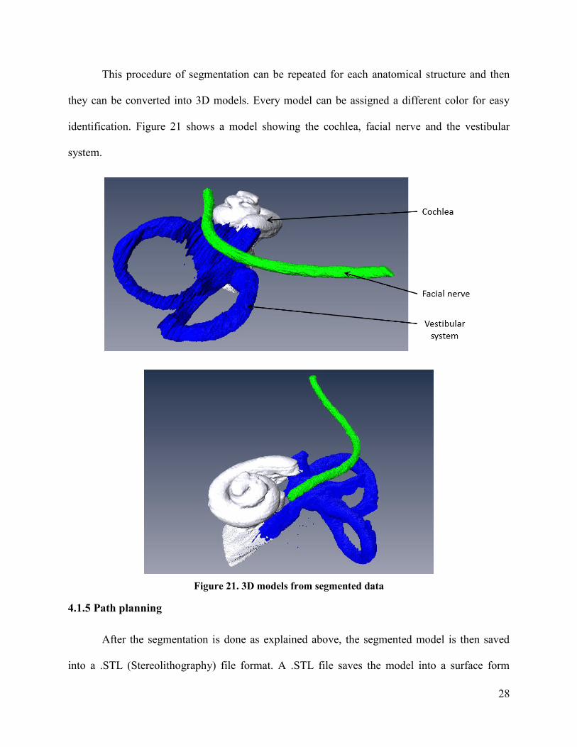
This procedure of segmentation can be repeated for each anatomical structure and then

they can be converted into 3D models. Every model can be assigned a different color for easy

identification. Figure 21 shows a model showing the cochlea, facial nerve and the vestibular

system.

Figure 21. 3D models from segmented data

4.1.5 Path planning

After the segmentation is done as explained above, the segmented model is then saved

into a .STL (Stereolithography) file format. A .STL file saves the model into a surface form

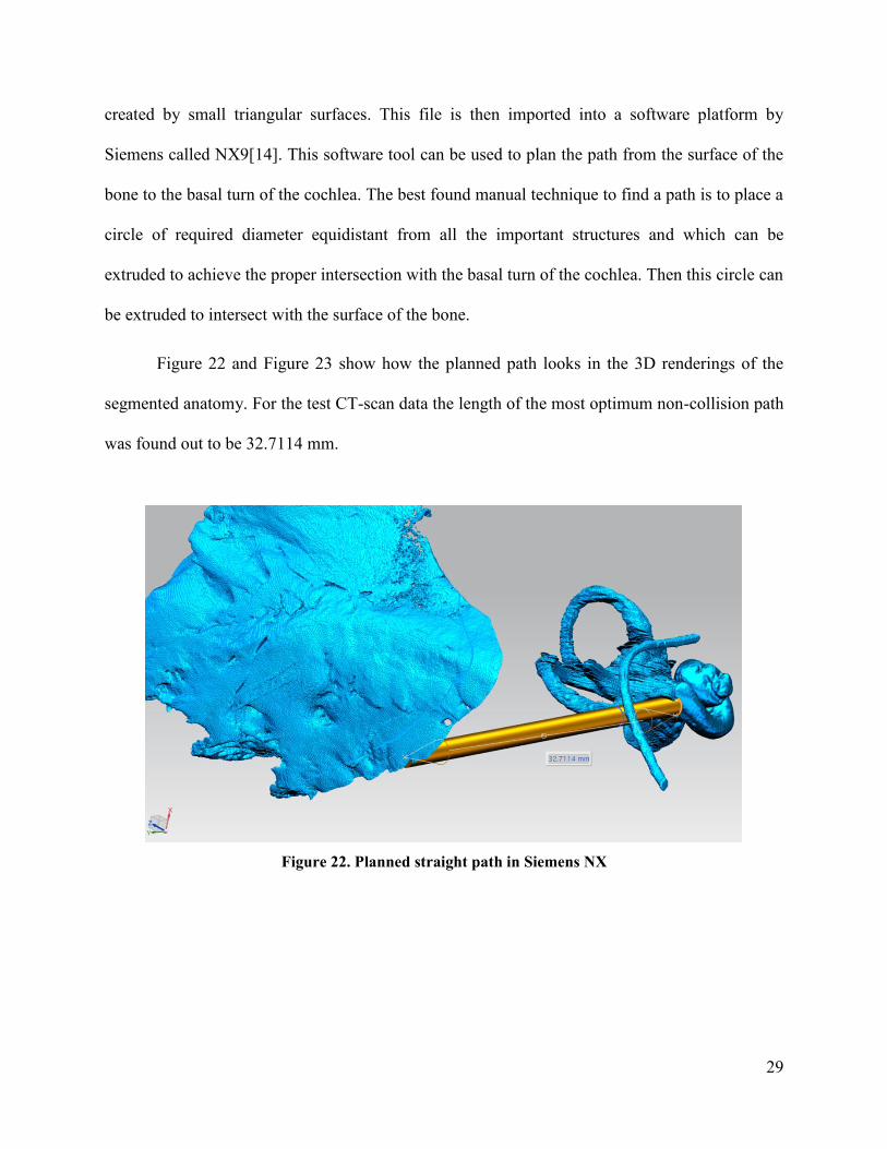
29

created by small triangular surfaces. This file is then imported into a software platform by

Siemens called NX9[14]. This software tool can be used to plan the path from the surface of the

bone to the basal turn of the cochlea. The best found manual technique to find a path is to place a

circle of required diameter equidistant from all the important structures and which can be

extruded to achieve the proper intersection with the basal turn of the cochlea. Then this circle can

be extruded to intersect with the surface of the bone.

Figure 22 and Figure 23 show how the planned path looks in the 3D renderings of the

segmented anatomy. For the test CT-scan data the length of the most optimum non-collision path

was found out to be 32.7114 mm.

Figure 22. Planned straight path in Siemens NX

30

Figure 23. Planned straight path in Siemens NX

4.2 Stewart platform actuator

4.2.1 Construction of the Stewart Platform Actuator

The work for this Thesis was a continuation of a prototype design and build for the

Stewart Platform Actuator. It was done by David Cowens, an undergraduate student in Bio-

medical Engineering. Figure 24 shows his final model and the actual build for the actuator.

31

Figure 24. Initial design and build for the Stewart Platform Actuator

Some of the important features of this design were

1) Top and bottom plate were of the same diameter, 5 inch each.

2) Tool holder was attached to the top plate.

3) Tool was clamped in the tool holder and protruded through the bottom plate.

4) 6 Faulhaber LM 2070 Linear DC servomotors [18] were used as linear actuators on every leg.

5) 12 spherical joints at the top and bottom ends of every leg connected the top and bottom plate

to all the actuators.

6) Each linear motor was operated by MCLM3006 Motion Controller [19] connected to the

computer running MATLAB [20] using USB interface.

As the base and the top plate were of the same size, at higher angles of tilt for the tool the

actuator used to fall off on that side. Also the actuator needed an arrangement to facilitate the

32

easy positioning on patient’s skull while supporting the weight of the whole mechanism. The

solution to these problems was to design a new base to spread out the joints, making the actuator

more stable and also to make provisions for positioning the actuator.

Figure 25. Revised design for the Stewart Platform Actuator

Figure 26. Revised build of the Stewart Platform Actuator

33

The latest version of this actuator, shown in Figure 25, consists of 6 aluminum bars,

clamped to square 24 x 24 inch 1/4th inch aluminum plate, forming a hexagonal shape. The

diameter of the inner circle of this hexagon is 15 inches. Alternate bars carry two of the six

spherical joints at a distance of 1/2 inch on either side of their center. All six legs are attached

between the spherical joints on the platform and the top plate and can be actuated by LM 2070

Linear DC servomotors. There is a circular hole of diameter 1.5 inches in the center of the

aluminum plate from which the tool attached to the top platform protrudes. 3 M2.5 holes are

tapped at a diameter of 2 inches to allow screws to go through the base plate and complete the

assembly for the positioning of the platform. Figure 25 shows the Solidworks model and Figure

26 shows the actual build of the revised Stewart Platform actuator.

4.2.2 Algorithm for the Stewart Platform actuator

The aim of this algorithm is to operate the actuator in following steps as shown in Figure

27.

1) Bring the tool tip to origin of reference frame (O), which is at the center of joints on bottom

plate, from its initial position.

2) Bring the tool tip to point P1 (the start point for the path) and align it in the direction of P2 (the

end point for the path).

3) Push the tool tip from point P1 to P2 in a straight line to complete the drilling operation.

4) Retract the tool to point P1 from point P2 in a straight line.

5) Bring the tool tip back to the origin of the reference frame.

34

Figure 27. Path to be followed by the tool tip

To complete this procedure two approaches can be used.

Approach I

1) Calculate the co-ordinates for the joints on the top and bottom plate at the initial actuation of

the linear motors with respect to the reference frame. Determine the co-ordinates of the tool tip

with respect to reference frame at the initial actuation of the linear motors.

2) Determine the positions for the start and end points from the path planned. Let these positions

be P1 and P2 whose co-ordinates with respect to the reference frame are [x1, y1, z1] and [x2, y2, z2]

respectively.

3) Calculate the vector P1P2[x12, y12, z12] = P1 - P2 and then use that vector to calculate the Roll

(γ), Pitch (β) and Yaw (α) using equation (1).

35

4) Use these angles to calculate the transformation matrices T1 and T2 from the equations (2) and

(3).

5) Calculate the co-ordinates of the top joints for the tool tip positions O, P1 and P2 from

equation (4).

6) Use the distance formula from equation (5) to calculate the actuations for each motor to cause

the transitions between different positions.

7) The magnetic pitch for the DC motors is 24 mm which requires 3000 pulses per revolution.

So, the controller has to provide 125 pulses per mm of actuation. This data is used to convert the

actuations into pulses.

8) For the transitions between the initial position, point O and P1 direct actuations are used as the

aim is just to achieve those positions and the path travelled is not important.

9) For the path P1P2 the actuations for each linear motor are used to setup limits or stops at the

respective positions and then each motor is actuated at respective velocities so that they reach the

end point at the exact same time. This results in the tool tip following a perfectly straight path

P1P2.

Approach II

Steps 1 to 7 are similar to the ones used in Approach I

8) Divide the actuations of each motor required to transition from point O to P1 and P1 to P2 into

100 equal parts each.

9) Actuate all the motors at the same time in 100 steps to transition between different points. The

accuracy can further be increased by increasing these steps for longer tool travel.

36

4.2.3 Commands for motor control

MCLM3006 Motion Controllers interfaced with a computer running MATLAB are used

to control each of the LM 2070 Linear DC servomotors. The commands that are sent to the

controllers for different operations of the motors are listed here.

Command Argument Function Description

EN - Enable/engage drive Activate drive

DI - Disable Drive Deactivate drive

LA Value Load Absolute Position Load new absolute target position

LR Value Load Relative Position Load new relative target position, in

relation to last started target position.

M - Initiate Motion Activate position control and start

positioning

HO -/value Define Home Position

Without argument: Set actual position to

0.

With argument: Set actual position to

specified value.

V Value Select Velocity Mode

Activate velocity mode and set specified

value as target velocity (velocity

control). Unit: rpm

SP Value Load Maximum Speed Load maximum speed (here: Target

velocity at 10 V). Unit: rpm

MV Value Minimum Velocity Specifies the lowest velocity Unit: rpm

AC Value Load Command

Acceleration

Load acceleration value (1/s²). Value: 0

… 30 000

DEC Value Load Command

Acceleration

Load deceleration value (1/s²). Value: 0

… 30 000

SP Value Load Maximum Speed Load maximum speed (rpm). Value: 0

… 30 000

37

The magnetic pitch of all motors is 24 mm for 3000 pulses sent from the controllers. So,

1 mm motion of the motor corresponds to 125 pulses from the controllers. Using these

commands the required motion can be achieved for the motors. A PID controller is implemented

by the controllers and its performance was found to be satisfactory enough to not implement a

new controller for our requirements.

4.3 Non-invasive registration

4.3.1 Laser Scanning and Image acquisition

3D laser scanning works on the principle of triangulation[21] in which a line is projected

by a laser over an object and the image is captured by a camera whose axis is at an angle to the

plane of the line created by the line laser. The distance of the object from the system can then be

calculated by trigonometry as long as the distances between the camera and the laser system are

known. In the laser scanning techniques used here, a line laser pointer is attached to the top

platform of the Stewart platform actuator pointing downwards on the work surface. Figure 28

shows the laser pointer used for this purpose and the laser line generated by it on an object.

Figure 28. (a) Line Laser Pointer (b) Line Generated on an Object

38

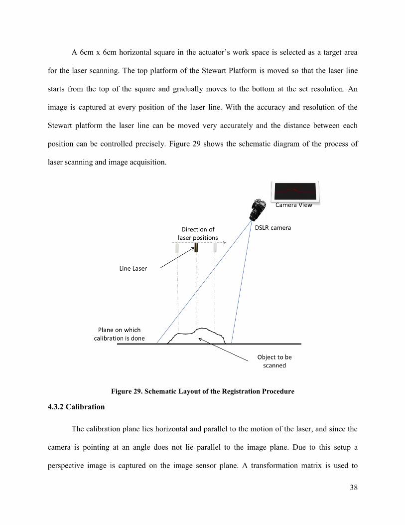
A 6cm x 6cm horizontal square in the actuator’s work space is selected as a target area

for the laser scanning. The top platform of the Stewart Platform is moved so that the laser line

starts from the top of the square and gradually moves to the bottom at the set resolution. An

image is captured at every position of the laser line. With the accuracy and resolution of the

Stewart platform the laser line can be moved very accurately and the distance between each

position can be controlled precisely. Figure 29 shows the schematic diagram of the process of

laser scanning and image acquisition.

Figure 29. Schematic Layout of the Registration Procedure

4.3.2 Calibration

The calibration plane lies horizontal and parallel to the motion of the laser, and since the

camera is pointing at an angle does not lie parallel to the image plane. Due to this setup a

perspective image is captured on the image sensor plane. A transformation matrix is used to

39

determine the exact location of the point captured by every image pixel with respect to the

calibration plane. Figure 30 shows how a square grid placed on the calibration plane looks from

the camera view. The distances for every point on the square grid are known and applying a

transform from the image plane to the calibration plane will give the exact co-ordinates of the

point with respect to the calibration plane. A 6cm x 6cm square grid is used as reference

geometry in the calibration plane to calculate the transformation matrix. The image of this grid is

captured by the camera as shown in the Figure 30(a) and is used as a calibration image. Also to

calibrate the workspace in the direction normal to the calibration plane (height) a 10 mm high

object is kept in the workspace and images are captured of the laser line at each position. The

step by step algorithm used for calculating the transformation matrix and the height calibration is

explained below. This algorithm is implemented in MATLAB and uses some of the pre-loaded

functions and toolboxes to accomplish some of the tasks. These functions will be explained at the

respective steps.

Figure 30. (a) 6cm x 6cm grid used for calibration (b) Image of the grid captured by the camera

40

1) The image is cropped so that only the grid is visible to avoid any rogue lines to be detected in

the further steps.

2) The image is then converted to a logical black and white image where the blacks are denoted

by ‘0’ and whites by ‘1’. A suitable threshold is selected so that all the pixels on the grid lines

are classified as blacks. Then this image is inverted to get an image which has pixels with

intensity ‘1’ representing all the grid lines. Figure 31(a) shows the converted image.

3) All the lines in this converted image are detected by using the Hough transform[22] from the

MATLAB image processing toolbox[23] and the slopes and y-intercepts for the top 14 Hough

lines are recorded. Hough transform is a technique used to isolate features of a particular shape

from a binary image. To detect lines in an image, angles (θ) and lengths (ρ) of perpendiculars

from the origin to all the possible lines in the image plane are decided. For each of these lines the

number of points lying on them is recorded. Figure 31(b) shows the plot of ρ vs θ and also the 14

lines with highest number of points on them. The equations for these lines can be calculated by

using

𝑥 cos 𝜃 + 𝑦 sin 𝜃 = 𝜌

41

Figure 31. (a) Binary Image of the grid (b) Plot for the Hough lines

4) These equations are then matched to the respective lines by taking manual inputs by

highlighting each line in the image and asking for the user input for the number of line. The lines

are numbered from 1 to 7 for right to left and 8 to 14 for top to bottom.

5) Pixel co-ordinates for each of the intersection points on the grid are then calculated by using

the geometry of the lines.

6) Homography function, by Kovesi[24], is used to calculate the transformation matrix which

can calculate the co-ordinates of points on the calibration plane from the pixel co-ordinates in the

image. Homography can be simply defined as; given co-ordinates of four points on one plane

there exists a relationship that transforms them into the corresponding four points in another

plane. In this case the four points lie on the corners of the grid in the perspective image plane and

the calibration plane. Homography function takes the co-ordinates of points on both planes and

outputs a 3x3 transformation matrix called the Homography transform. Let’s denote this matrix

by HG. The co-ordinates for the grid corners in the image plane are calculated in the previous

step and the co-ordinate of the grid corners in the calibration are already known and are shown in

Figure 30(a).

42

7) The images from the image sequence captured for height calibration are loaded on by one.

Each image is cropped at the exact pixels at which the calibration image was cropped at and the

pixels with highest intensity which represent the 10 mm height are recorded. Also the pixels with

highest intensity representing the base height are recorded. Both of these heights are represented

by y1 and y2 respectively as shown in the Figure 32. Calibration image for 10 mm height at nth

laser line position Now the 10mm height for nth laser line position is calculated by

ℎ𝑡𝑛 = 𝑦2 − 𝑦1

Figure 32. Calibration image for 10 mm height at nth laser line position

The ultimate aim of the calibration routine is to calculate the Homography transformation

matrix, the equations of all the grid lines in the calibration image and to determine the number of

pixels by which the laser line is shifted for a height of 10 mm for each of the laser line positions.

All of these are used during the point cloud creation which is explained next.

43

4.3.3 Point cloud creation from the captured image sequence

Point cloud is created by determining the X, Y and Z co-ordinates of all the points on the

surface of the object with respect to some reference co-ordinate system. In this technique the

point cloud is calculated with reference to the (0, 0) co-ordinate of the grid in the calibration

plane. The aim is to extract each slice, spaced at a preset distance, of the surface from every

image. If the resolution is preset at 0.1 mm the total images to cover the 6 cms of the grid will be

61 and 121 images for 0.05 mm and so on. From the sequence of images the steps in which the

co-ordinates of the points are calculated are explained below.

1) The images are loaded one after another and are processed individually before loding the next

image in the sequence. Following steps are explained for one image (let’s say nth which also

represents the nth laser line position) and repeated for other images.

2) The image is cropped at the exact pixels at which the calibration image was cropped at. Figure

33 shows a cropped sample image.

44

Figure 33. Cropped sample Image from the Image sequence

3) MATLAB image processing toolbox[23] is used to the isolate the intensities of the red color

from this image since a red laser line was used while scanning.

4) The y co-ordinates of the points with the maximum intensity for every column are identified.

Also, the y co-ordinates for the pixels that represent the base height are recorded. The height of

the point with maximum intensity from the base height point in pixels is calculated as the

difference of the above two. Let’s denote this height for this point in the kth column in the nth

image by hnk.

5) For a particular point k with high intensity in the nth image we have the X and Y pixel co-

ordinates(Xpx and Ypx), height in pixels hnk, Y-co-ordinate of the base laser line on the calibration

plane (which is basically n times the preset resolution of laser scanning) , the 10 mm calibration

height htn and the Homography Transform matrix HG.

45

6) The X, Y and Z co-ordinates for a point on the point cloud (Xkpc, Yk

pc ,Zkpc) are calculated in

the following way.

[𝑋𝑘

𝑝𝑐

𝑌𝑌𝑍𝑍

]

3𝑥1

= [𝐻𝐺]3𝑥3 × [

𝑋𝑝𝑥

𝑌𝑝𝑥

1

]

3𝑥1

Where YY and ZZ are discarded and just Xkpc is recorded in mm.

𝑌𝑘𝑝𝑐 = 𝑛 × 𝑟𝑒𝑠𝑜𝑙𝑢𝑡𝑖𝑜𝑛 𝑜𝑓 𝑡ℎ𝑒 𝑙𝑎𝑠𝑒𝑟 𝑠𝑐𝑎𝑛 𝑖𝑛 𝑚𝑚

𝑍𝑘𝑝𝑐 =

ℎ𝑛𝑘

ℎ𝑡𝑛 × 10 𝑚𝑚

7) The same procedure is repeated for all the images in the image sequence and X, Y and Z co-

ordinates for all the points are determined.

This algorithm is implemented in MATLAB and the co-ordinates of the points are

exported in a text file. The format of this text file is the co-ordinates of each point, separated by a

single space, on a new line. The format of this file is then changed to ‘.xyz’ so that it can be

imported into Meshlab[25] for further editing. The point cloud can be visualized and rogue noisy

points can be selected and deleted in Meshlab. The finished point cloud can again be exported

and converted to a text file.

4.3.4 Registration of the Point Cloud

Registration of a point cloud means to determine the translational and rotational

transformation through which one point cloud has to undergo to best match the reference. The

reference can be a CAD model and the point cloud can be a laser scan data. To demonstrate the

registration of point cloud data from the laser scanning done by the Stewart Platform actuator a

46

simple Iterative Closest Point(ICP) Algorithm[26] is used to find out the angle of rotation

between two point clouds generated of the same object kept at different positions.

In the ICP algorithm, one point cloud is fixed and is used as a reference while the other

one is rotated at some prefixed angular steps. At each position a cost function is calculated by

randomly sampling few points from each point cloud. Let’s say n points are sampled from each

point cloud.

𝐼𝐶𝑃 𝐶𝑜𝑠𝑡 𝐹𝑢𝑛𝑐𝑡𝑖𝑜𝑛 = ∑𝐷𝑖𝑠𝑡𝑎𝑛𝑐𝑒 𝑏𝑒𝑡𝑤𝑒𝑒𝑛 𝑡ℎ𝑒 𝑝𝑜𝑖𝑛𝑡 𝑎𝑛𝑑 𝑡ℎ𝑒

𝑐𝑙𝑜𝑠𝑒𝑠𝑡 𝑝𝑜𝑖𝑛𝑡 𝑡𝑜 𝑖𝑡 𝑜𝑛 𝑡ℎ𝑒 𝑟𝑒𝑓𝑒𝑟𝑒𝑛𝑐𝑒 𝑃𝐶𝑛

The angle of rotation for registration is represented by the lowers value of the ICP cost

function. This algorithm is implemented in MATLAB and takes the text files of two point clouds

as an input and gives out the plot of the ICP cost function.

47

Chapter 5. Tests and Results

5.1 Test for the accuracy of the Stewart Platform Actuator

5.1.1 Test setup

Figure 34 shows the anchor screws fixed into the faux bone sheet and how the faux bone

sheet is positioned below the actuator platform. Since the faux bone has a plane surface anchor

screws are directly attached to the actuator platform without the plastic printed fixture assembly.

While carrying out this test on a cadaveric sample there will be a fixture assembly present, this

will give us the versatility to fix the anchor screws at suitable positions and angles.

Figure 34. Test setup

To test the accuracy of the Stewart Platform actuator the faux bone sheets were

positioned as discussed in the Test setup and two tests were done. 1) Test for angular accuracy

and 2) Test for positional accuracy. Since the drill attachment we have is not yet suitable for

drilling more than 15 mm in a straight line these initial tests were done. A suitable drill

48

attachment needs to be selected and obtained which will be more suitable to complete a straight

hole of 35 mm. The kind of burr of the tool tip will also be an important factor to reduce the

vibrations.

5.1.2 Test for Angular Accuracy

This test was done to check how well the actuator performs in drilling holes at different

angles. 10 mm deep holes were drilled at 0° and 5° angles. Figure 35 shows the results for the 0°

and 5° angles. The actuator performed almost perfectly in drilling these holes and the

performance was satisfactory.

Figure 35. Results for the Angular Accuracy test (0 and 5 degrees)

49

5.1.3 Test for Positional Accuracy

To test the positional accuracy of the actuator 13 holes were drilled in a faux bone sheet

at a depth of 2 mm each. Figure 36. Plan for the Positional Accuracy Test shows the co-ordinates of

the different holes on the surface of the faux bone sheet. Figure 37 shows the results of this test

with the expected positions of the holes.

Figure 36. Plan for the Positional Accuracy Test

Figure 37. Results for the Positional Accuracy Test

50

Visually inspecting the square grid pattern made by the drilled holes, it can clearly be

observed that they are exactly spaced from each other but rotated slightly in the anti-clockwise

direction. This could have happened due to errors in initial calibration of the actuator. Other

errors could have been introduced by the manufacturing errors in the actuator components.

According to Schipper J. et. al. [27], the required accuracy for a surgical drill for CI should be

below 0.5 mm and with certain improvements that accuracy can be achieved with the actuator

that we have built.

Following table shows the errors in X and Y direction for each of the holes.

Table 2. Positional Errors

Position Number Desired Co-ordinates Error in X direction Error in Y direction

1 (0, 0) 0 mm 0 mm

2 (10, 0) 0 mm 0.5 mm

3 (10, 10) 0.5 mm 0 mm

4 (0, 10) 0 mm 0 mm

5 (-10, 10) -1 mm -1 mm

6 (-10, 0) 0 mm -1 mm

7 (-10, -10) 1 mm 0 mm

8 (0, -10) 1 mm 0 mm

9 (10, -10) 0.5 mm 1 mm

10 (5, 5) 0.5 mm 0 mm

11 (-5, 5) 0 mm 0.5 mm

12 (-5, -5) -0.5 mm 0 mm

13 (5, -5) 0 mm 0.5 mm

51

5.2 Test for the accuracy of laser scanning and registration

To test out the procedure of laser scanning, point cloud creation and registration an object

was scanned at different angular positions. Figure 38 and Figure 39 (a) shows the default position

of the object (Position 1) and all other positions that are registered to the default position. The

resolution of the laser scan was set at 1 mm and a sequence of 61 images was recorded for the 10

mm height calibration and for each of the positions of the object.

Figure 38. Different Positions for the test object (1)Default position [0°] (2) Position 2 [90°] (3)

Position 3 [45°]

52

Figure 39. Different Positions for the test object (4) Position 4 [135°] (5) Position 5 [180°] (6)

Position 5 [30°] (7) Position 5 [60°]

53

Point clouds for each of the image sequence at every position were extracted using the

MATLAB codes and were recorded in a text file. These text files were then converted to a ‘.xyz’

file and imported into Meshlab for visualization and cleaning. Figure 38 (b) shows the raw point

clouds created and exported from MATLAB and Figure 38 (c) shows the cleaned point clouds for

the corresponding positions of the test object visualized in Meshlab.

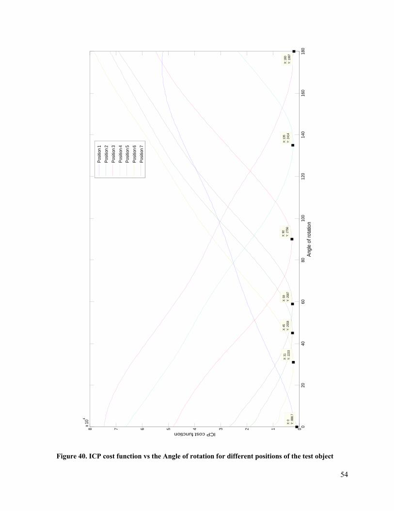
ICP algorithm explained earlier is applied to each of the position compared to the default

position. The cost functions for each of these comparisons are plotted against the angle of

rotation. Figure 40 shows the ICP cost function for every position with their minimum values

marked. These minimum values represent the results for the estimated angle of rotation from the

comparison of point clouds and in turn the registration of the point clouds.

Table 3. Estimated angles of rotation from the registration data

Position Estimated angle from the point

cloud registration Error

0° 0° 0

30° 31° 1°

45° 45° 0

60° 59° -1°

90° 90° 0

135° 135° 0

180° 180° 0

Table 3 summarizes the estimated values for the angle of rotation from the registration

data and compares them with the actual position of the object. It can be observed that the

estimation is fairly accurate.

54

02

04

06

08

01

00

12

01

40

16

01

80

012345678x

10

4

X: 0

Y: 888.7

Ang

le o

f ro

tatio

n

ICP cost function

X: 31

Y: 2233

X: 45

Y: 2558

X: 59

Y: 2587

X: 90

Y: 2756

X: 135

Y: 2414

X: 180

Y: 1997

Po

sitio

n 1

Po

sitio

n 2

Po

sitio

n 3

Po

sitio

n 4

Po

sitio

n 5

Po

sitio

n 6

Po

sitio

n 7

Figure 40. ICP cost function vs the Angle of rotation for different positions of the test object

55

5.3 Test for registration of points tracked by the tool tip

In this test, location for four points on an object was fed to the actuator. Then the object

was rotated at different positions and from the laser scanned point cloud data the angle of

rotation was determined. This angle was then used to transform the points tracked by the

actuator. For each angular position of the test object the actuator was made to track the same

points based on the registration data. Figure 41 shows the position of the tool tip at the four points

on the test object. Figure 42, Figure 43, Figure 44 and Figure 45 show the position of the tool tip

calculated from the registration data of the laser scan.

It can be clearly observed that the tooltip attached to the actuator is able to track the

points on the object from the laser scan registration data.

Figure 41. Four input points on the test object

56

Figure 42. Points tracked by the actuator using the registration data from the laser scan for 45°

rotation

Figure 43. Points tracked by the actuator using the registration data from the laser scan for 90°

rotation

57

Figure 44. Points tracked by the actuator using the registration data from the laser scan for 135°

rotation

Figure 45. Points tracked by the actuator using the registration data from the laser scan for 180°

rotation

58

Chapter 6. Conclusion and Future Work

The research presents a setup for performing direct access cochlear implant. The process

of identifying and segmenting a CT-scan data into important anatomical structures has been

demonstrated. Determination of a straight no-collision path from the surface of the mastoid bone

to the basal turn of the cochlea has also been done. The technique for positioning the actuator

over the patient’s skull using anchor screws and non-invasively has also been documented. The

earlier version of the Stewart Platform actuator has been successfully modified to suit our

purpose. From the results of Chapter 5, it can be concluded that with certain improvements this

actuator can be made suitable for CI.

It can be concluded from the path planning methodology that, a straight line path can be

planned for a direct access cochlear implant from CT-scan images using the software Amira. It

can also be concluded from the results of the actuator testing that, with certain improvements in

calibration the actuator can provide the required accuracy and precision for direct access

cochlear implantation. Finally, the 3D laser scanning registration technique discussed here is a

feasible solution to make the positioning of the actuator non-invasive and further work needs to

be conducted to explore this opportunity.

The advantages of using this procedure are that the Stewart Platform actuator is designed

specifically for cochlear implantation surgery and other surgeries requiring drilling through the

temporal bone. Because other robotic surgical systems are designed for laparoscopic surgery, and

are meant to be encompassing of a wide variety of surgeries, they are not ideal for temporal bone

surgery. They are also extremely expensive. By designing a device specifically for Temporal

Bone Surgery, we will be able to optimize the device’s effectiveness and minimize the cost.

59

Future work for this project will be carried out during my doctoral studies. Further work

in selecting a suitable drill attachment needs to be done. Also cadaveric tests need to be done to

prove the feasibility of this procedure. More focus will be on improving the non-invasive

positioning techniques. The non-invasive registration technique needs to be improved to work

with translational and rotational transformations in all directions. Registering the actuator system

with a traditional motion tracking system will also open a new avenue of opportunities which

need to be explored. Focus will also be kept on making the actuator system semi-autonomic with

haptic feedback devices, that way transferring a part of the control to the surgeon.

60

Chapter 7. References

[1] National Institute on Deafness and Other Communication Disorders, “Cochlear implants,”

National Institute on Deafness and Other Communication Disorders. [Online]. Available:

http://www.nidcd.nih.gov/health/hearing/pages/coch.aspx. [Accessed: 15-Apr-2014].

[2] G. M. Clark, B. C. Pyman, and Q. R. Bailey, “The surgery for multiple-electrode cochlear

implantations,” J. Laryngol. Otol., vol. 93, no. 03, pp. 215–223, 1979.

[3] “Cochlear Implants- Hearing Loss Association of America.” [Online]. Available:

http://www.hearingloss.org/content/cochlear-implants. [Accessed: 29-Apr-2014].

[4] “Hearing Loss Stats « Cochlear Implant Online.” .

[5] T. Kubo, S. Matsuura, and T. Iwaki, “Complications of cochlear implant surgery,” Oper.

Tech. Otolaryngol.-Head Neck Surg., vol. 16, no. 2, pp. 154–158, Jun. 2005.

[6] O. Majdani, T. S. Rau, S. Baron, H. Eilers, C. Baier, B. Heimann, T. Ortmaier, S. Bartling,

T. Lenarz, and M. Leinung, “A robot-guided minimally invasive approach for cochlear

implant surgery: preliminary results of a temporal bone study,” Int. J. Comput. Assist.

Radiol. Surg., vol. 4, no. 5, pp. 475–486, Sep. 2009.

[7] B. Bell, C. Stieger, N. Gerber, A. Arnold, C. Nauer, V. Hamacher, M. Kompis, L. Nolte, M.

Caversaccio, and S. Weber, “A self-developed and constructed robot for minimally invasive

cochlear implantation,” Acta Otolaryngol. (Stockh.), vol. 132, no. 4, pp. 355–360, Apr.

2012.

[8] R. F. Labadie, P. Chodhury, E. Cetinkaya, R. Balachandran, D. S. Haynes, M. R. Fenlon,

A. S. Jusczyzck, and J. M. Fitzpatrick, “Minimally invasive, image-guided, facial-recess

approach to the middle ear: demonstration of the concept of percutaneous cochlear access

in vitro,” Otol. Neurotol. Off. Publ. Am. Otol. Soc. Am. Neurotol. Soc. Eur. Acad. Otol.

Neurotol., vol. 26, no. 4, pp. 557–562, Jul. 2005.

[9] J. H. Noble, F. M. Warren, R. F. Labadie, B. Dawant, and J. M. Fitzpatrick, “Determination

of drill paths for percutaneous cochlear access accounting for target positioning,” 2007, pp.

650925–650925–10.

[10] “iPlan CMF—Straightforward Planning and Navigation,” Brainlab. [Online]. Available:

https://www.brainlab.com/surgery-products/overview-ent-cmf-products/iplan-cmf-

straightforward-planning-and-navigation/. [Accessed: 14-May-2014].

[11] “CT scan - Mayo Clinic.” [Online]. Available: http://www.mayoclinic.org/tests-

procedures/ct-scan/basics/definition/prc-20014610. [Accessed: 18-May-2015].

[12] “Amira | FEI Visualization Sciences Group.” [Online]. Available:

http://www.vsg3d.com/amira/overview. [Accessed: 13-May-2014].

[13] “The Radiology Assistant : Temporal bone - Anatomy.” [Online]. Available:

http://www.radiologyassistant.nl/en/p43facba0911f5/temporal-bone-anatomy.html.

[Accessed: 13-May-2014].

61

[14] “Accelerate Product Development with NX 9: Siemens PLM Software.” [Online].

Available: http://www.plm.automation.siemens.com/en_us/products/nx/9/index.shtml.

[Accessed: 12-Jun-2014].

[15] D. Stewart, “A Platform with Six Degrees of Freedom,” Proc. Inst. Mech. Eng., vol. 180,

no. 1, pp. 371–386, Jun. 1965.

[16] G. G. Slabaugh, “Computing Euler angles from a rotation matrix.”

[17] G. S. Phillips, S. E. LoGerfo, M. L. Richardson, and Y. Anzai, “Interactive web-based

learning module on CT of the temporal bone: anatomy and pathology,” Radiogr. Rev. Publ.

Radiol. Soc. N. Am. Inc, vol. 32, no. 3, pp. E85–105, Jun. 2012.

[18] “Linear DC Servomotors – QUICKSHAFT® Data Sheet | MICROMO.” [Online].

Available: http://www.micromo.com/quickshaft-data-sheet.aspx. [Accessed: 23-May-

2014].

[19] “FAULHABER MCLM 3006 S CF Motion controller.” [Online]. Available:

http://www.micromo.com/manuals/sites/en/steuerungen/mclm_3006_s_cf.html. [Accessed:

24-May-2014].

[20] “MATLAB - The Language of Technical Computing.” [Online]. Available:

http://www.mathworks.com/products/matlab/. [Accessed: 24-May-2014].

[21] J. G. D. M. Franca, M. A. Gazziro, A. N. Ide, and J. H. Saito, “A 3D scanning system based

on laser triangulation and variable field of view,” in IEEE International Conference on

Image Processing, 2005. ICIP 2005, 2005, vol. 1, pp. I–425–8.

[22] “Hough transform - MATLAB hough.” [Online]. Available:

http://www.mathworks.com/help/images/ref/hough.html. [Accessed: 15-Mar-2015].

[23] “Image Processing Toolbox - MATLAB.” [Online]. Available:

http://www.mathworks.com/products/image/index-b.html. [Accessed: 15-Mar-2015].

[24] P. Kovesi, E.-J. Holden, and J. Wong, “Interactive multi-image blending for visualization

and interpretation,” Comput. Geosci., vol. 72, pp. 147–155, Nov. 2014.

[25] “MeshLab.” [Online]. Available: http://meshlab.sourceforge.net/. [Accessed: 17-Mar-

2015].

[26] P. J. Besl and N. D. McKay, “A method for registration of 3-D shapes,” IEEE Trans.

Pattern Anal. Mach. Intell., vol. 14, no. 2, pp. 239–256, Feb. 1992.

[27] P.-D. D. J. Schipper, T. Klenzner, A. Aschendorff, I. Arapakis, G. J. Ridder, and R. Laszig,

“Navigiert-kontrollierte Kochleostomie,” HNO, vol. 52, no. 4, pp. 329–335, Apr. 2004.