Stochastic Analysis and Optimization of Power …etheses.bham.ac.uk/3836/1/LI_12_PhD.pdfSTOCHASTIC ANALYSIS AND OPTIMIZATION OF POWER SYSTEM STEADYSTATE WITH WIND FARMS AND ELECTRIC

STOCHASTIC ANALYSIS AND

OPTIMIZATION OF POWER SYSTEM

STEADY-STATE WITH WIND FARMS

AND ELECTRIC VEHICLES by

GAN LI A thesis submitted to The University of Birmingham for the degree of DOCTOR OF PHILOSOPHY

School of Electronic, Electrical and Computer Engineering The University of Birmingham June 2012

University of Birmingham Research Archive

e-theses repository This unpublished thesis/dissertation is copyright of the author and/or third parties. The intellectual property rights of the author or third parties in respect of this work are as defined by The Copyright Designs and Patents Act 1988 or as modified by any successor legislation. Any use made of information contained in this thesis/dissertation must be in accordance with that legislation and must be properly acknowledged. Further distribution or reproduction in any format is prohibited without the permission of the copyright holder.

To my parents

ACKNOWLEDGEMENTS

First and foremost, I would like to express my sincere appreciation to my supervisor, Prof.

Xiao-Ping Zhang, for his support, guidance, inspiration and patience during my PhD study. I

have greatly benefited from his knowledge and experience.

I am also grateful to Associate Prof. Zhigang Wu and Associate Prof. Xuefeng Bai for their

support and advices on my research. Many thanks to Mr. Dechao Kong, Mr. Zhou Li and Mr.

Bo Fan for sharing their valuable ideas with me. I would also like to thank my dear colleagues

Miss Rui Shi, Mr. Jingchao Deng, Mr. Xuan Yang, and Mr. Suyang Zhou for their

discussions and kind assistance during my study.

Finally, I would like to thank my families and all my friends. Without their encouragement,

support and understanding, completion of my thesis would not be possible.

ABSTRACT

Since the end of last century, power systems are more often operating under highly stressed

and unpredictable conditions because of not only the market-oriented reform but also the

rising of renewable generation and electric vehicles. The uncertain factors resulting from

these changes lead to higher requirements for the reliability of power grids. In this situation,

conventional deterministic analysis and optimization methods cannot fulfil these requirements

very well, so stochastic analysis and optimization methods become more and more important.

This thesis tries to cover different aspects of stochastic analysis and optimization of the power

systems from a perspective of its steady state operation. Its main research topics consist of

four parts: deterministic power flow calculations, modelling of wind farm power output and

electric vehicle charging demand, probabilistic power flow calculations, as well as stochastic

optimal power flow. These different topics involve modelling, analysis and optimization,

which could establish a whole stochastic methodology of the power system with wind farms

and electric vehicles.

i

TABLE OF CONTENTS

CHAPTER 1 INTRODUCTION 1

1.1 Research Background 1

1.1.1 Energy and Environment 1

1.1.2 Wind Generation Development 2

1.1.3 Electric Vehicle Popularization 5

1.1.4 Challenges and Opportunities 8

1.2 Research Focuses of This Study 10

1.3 Literature Review 12

1.3.1 Deterministic AC Power Flow 12

1.3.2 Charging Demand of Electric Vehicles 16

1.3.3 Probabilistic Power Flow 18

1.3.4 Stochastic Optimal Power Flow 20

1.4 Thesis Outlines 22

CHAPTER 2 ACCELERATED NEWTON-RAPHSON POWER

FLOW 24

2.1 Introduction 24

2.2 Mathematical Formulation 25

2.2.1 AC Power Flow Formulation 25

2.2.2 Accelerated Newton-Raphson Power Flow 27

2.3 Algorithm Analysis 29

ii

2.3.1 Proof of Convergence Characteristics 29

2.3.2 Determining Optimal Parameter αk 32

2.3.3 Computational Complexity 33

2.3.4 Flowchart of ANR Power Flow 35

2.4 Case Studies 36

2.5 Chapter Summary 46

CHAPTER 3 PROBABILITY MODELS OF UNCERTAINTIES

IN POWER SYSTEMS 48

3.1 Introduction 48

3.2 Load and Generator 49

3.2.1 Load 49

3.2.2 Generator 50

3.3 Wind Farm 50

3.3.1 Power Output of Wind Generator 50

3.3.2 Randomness of Wind Speed 52

3.3.3 Generation of Wind Farm 53

3.4 Electric Vehicle 55

3.4.1 Main Factors of Electric Vehicle Charging 55

3.4.2 Charging Demand of Single Electric Vehicle 55

3.4.3 Charging Demand of Multiple Electric Vehicles 58

3.4.4 Different Categories of Electric Vehicles 61

3.4.5 Random Simulation of the Overall Charging Demand of Electric Vehicles 62

3.4.6 Distribution Fitting of the Overall Charging Demand of Electric Vehicles 62

iii

3.5 Correlation between Uncertainties 67


CHAPTER 4 ANALYTICAL PROBABILISTIC POWER

FLOW CALCULATIONS 69

4.1 Introduction 69

4.2 Main Probabilistic Power Flow Methods 70

4.2.1 Monte Carlo Simulation 70

4.2.2 Point Estimate Method 72

4.2.3 Cumulant Method 72

4.3 Probabilistic Power Flow Considering Correlation 73

4.3.1 Linearized Power Flow Model 73

4.3.2 Cumulant Based Probabilistic Power Flow 75

4.3.3 Treatment of Correlation between System Inputs 78

4.4 Case Studies 83

4.4.1 Comparison of Probabilistic Power Flow Methods 83

4.4.2 Validation of Electric Vehicle Charging Demand Model 88

4.4.3 Impact of Correlation on Probabilistic Power Flow 94


CHAPTER 5 CHANCE-CONSTRAINED STOCHASTIC

OPTIMAL POWER FLOW 100

5.1 Introduction 100

5.2 Mathematical Formulation 101

iv

5.2.1 Deterministic Optimal Power Flow 101

5.2.2 Stochastic Optimal Power Flow 103

5.3 Heuristic Solution Approach 105

5.3.1 Overall Procedure 105

5.3.2 Equivalence of Chance Constraint 106

5.3.3 Adjustment of Constraint Bound 108

5.3.4 Flowchart of Heuristic Solution Approach 109

5.4 Case Studies 110


CHAPTER 6 RESEARCH SUMMARY 120

6.1 Conclusion and Contribution 120

6.2 Future Research 122

APPENDIX MATHEMATICAL FUNDAMENTALS 124

1 Numerical Characteristics of Random Variable 124

1.1 Moment and Cumulant 124

1.2 Covariance and Correlation 129

2 Probability Distribution Function Approximation 132

2.1 Orthogonal Polynomial Approximation 132

2.2 Series Expansion Approximation 133

2.3 Staircase Function Approximation 139

3 Convolution of Probability Distributions 142

4 Common Probability Distributions 143

4.1 Continuous Probability Distribution 143

v

4.2 Discrete Probability Distribution 147

LIST OF PUBLICATIONS 149

LIST OF REFERENCES 150

vi

LIST OF FIGURES

Figure 1-1 World total installed wind power capacity (GW) 3

Figure 1-2 UK installed wind power capacity (MW) 4

Figure 1-3 UK offshore wind farms (Source: Crown Estate) 5

Figure 2-1 Flowchart of the ANR power flow calculations 36

Figure 2-2 Bus power mismatches on the IEEE 118-bus system under loading level 300% 42

Figure 2-3 The value of αk during the ANR iterations on the 1145-bus system (loading

level=150%) 45

Figure 2-4 The ANR1 iteration counts with different α0 values on the IEEE 118-bus system

(loading level: 300%) and on the 3141-bus system (loading level: 150%) 46

Figure 3-1 Typical power curve of a wind generator 51

Figure 3-2 Weibull distribution of yearly wind speed 53

Figure 3-3 Wake effect demonstration (Source: Riso National Laboratory, Denmark) 54

Figure 3-4 Sample histogram and probability density fitting (charging station) 65

Figure 3-5 K-S test for cumulative distribution fitting (charging station) 66

Figure 3-6 Sample histogram and probability density fitting (residential community) 66

Figure 3-7 K-S test for cumulative distribution fitting (residential community) 67

Figure 4-1 Cumulative distribution function of V11 85

Figure 4-2 Probability density function of P6-12 86

Figure 4-3 UKGDS-EHV5 urban distribution system 89

Figure 4-4 Cumulative distribution function of V7 91

Figure 4-5 Cumulative distribution function of P8-101 92

Figure 4-6 Cumulative distribution function of Q8-101 92

vii

Figure 4-7 Modified IEEE 14-bus test system 94

Figure 4-8 Probability density curve of wind farm power output at bus 8 96

Figure 4-9 Probability density function of V14 98

Figure 4-10 Cumulative distribution function of Q4-5 98

Figure 5-1 Computational procedure of the proposed S-OPF approach 109

Figure 5-2 Network diagram of a 5-bus system 110

Figure 5-3 Probability density curve of the voltage magnitude at bus 1 112

Figure 5-4 Probability density curve of the apparent power flow in branch 2-3 113

Figure 5-5 Network diagram of modified IEEE 118-bus system 114

Figure 5-6 Probability density curve of the voltage magnitude at bus 52 117

Figure 5-7 Probability density curve of the real power flow in branch 82-77 117

viii

LIST OF TABLES

Table 1-1 MW Load and Charging Projections for US Metro Areas in 2009 9

Table 2-1 Comparison of Power Flow Methods (Tolerance = 1e-6p.u., Load Level = 100%) 38

Table 2-2 Comparison of Power Flow Methods (Tolerance = 1e-6p.u., Load level = 140%) 39

Table 2-3 Comparison of Power Flow Methods with Bus Type Conversion (Tolerance = 1e-

6p.u., Load level = 100%) 40

Table 2-4 Comparison of Power Flow Methods under Different Loading Levels (Tolerance =

1e-6p.u.) 41

Table 2-5 Comparison of Power Flow Methods with Different Convergence Tolerance (Load

level = 100%) 43

Table 2-6 N-1 Verification on the IEEE 118-Bus System (Total Case = 177, Loading Level =

300%, Tolerance = 1e-6p.u.) 44

Table 2-7 N-1 Verification on the 3141-Bus System (Total Case = 2404, Loading Level =

150%, Tolerance = 1e-6p.u.) 44

Table 3-1 CBat

Range of Each PHEV Class 61

Table 3-2 Market Share of Each PHEV Class 61

Table 3-3 Em Parameters of Each PHEV Class 63

Table 3-4 kEV

Range of Each PHEV Class 63

Table 3-5 Queue Model Parameters 64

Table 4-1 Probabilistic Data of the IEEE 14-Bus Test System 83

Table 4-2 Mean and Standard Deviation of the IEEE 14-Bus Test System 84

Table 4-3 Mean and Standard Deviation of the IEEE 118-Bus Test System 86

Table 4-4 Average Error of the IEEE 118-Bus System at Different Load Variation Levels 87

ix

Table 4-5 Computation Time Comparison (in Seconds) 88

Table 4-6 Gaussian Charging Demand Parameters 89

Table 4-7 Weibull Charging Demand Parameters 90

Table 4-8 Average and Maximum Relative Error 90

Table 4-9 Probabilistic Load Data in the IEEE 14-Bus Test System 95

Table 4-10 Average Relative Error in Percentage 97

Table 5-1 Generator Cost Coefficients 110

Table 5-2 Results Comparison between S-OPF and D-OPF 111

Table 5-3 Wind Farm Data included in Modified IEEE 118-Bus System 114

Table 5-4 Iteration Information during S-OPF Solution 116

Table 5-5 Results Comparison under Different Constraint Probabilities 118

Table 5-6 Results Comparison under Different Load Variation Coefficients 119

x

LIST OF ABBREVIATIONS

ANR Accelerated Newton-Raphson power flow

FNR Fixed Newton-Raphson power flow

NR Newton-Raphson power flow

FD Fast Decoupled power flow

MRV Modifying right-hand-side vector

LDS Large diagonal strategy

FOR Forced outage rate

i.i.d. Independent, identically distributed

PPF Probabilistic power flow

CM Cumulant method

PEM Point estimate method

MCS Monte Carlo simulation

OPF Optimal power flow

D-OPF Deterministic optimal power flow

S-OPF Stochastic optimal power flow

1

CHAPTER 1 INTRODUCTION

1.1 Research Background

1.1.1 Energy and Environment

In the 21st century, our modern industry still relies on the fossil fuels, e.g. oil, gas, coal etc.,

as the dominant energy source. However, the exploitation and utilization of fossil fuels brings

negative impact on the environment, such as air pollution, greenhouse effect, extreme climate

and so on. The developed countries have to spend a lot of resources and time treating the

environmental problems left over during their industrialization process, while developing

countries are also troubled by the contradiction between environment protection and

economic development. On the other hand, the limited mineable reserves of fossil fuels and

their difference in regional distribution lead to worldwide concerns about energy security,

especially after three oil crises successively occurred in the mid and late 20th century [1].

Since the last decade of the 20th century, as the depletion trend of fossil fuels becomes widely

recognized along with the environmental challenge mainly due to global warming resulting

from excessive greenhouse gas emissions, the international community has reached an

agreement that it is necessary to reform the existing mode of production and consumption,

which excessively relies on fossil fuels, to a sustainable mode with cleaner alternative energy

and less greenhouse gas emissions [2]. From the energy supply side, the large scale

exploitation of renewable energy generation, such as solar energy, tidal energy, and especially

wind energy, is developing very fast and renewable energy sources have taken an important

role in the supply of energy [3]; on the energy demand side, electric vehicles are becoming

popular because of their high energy efficiency and low off-gas emissions, and an emerging

2

marketplace of electric vehicles is forming in both developing countries and developed

countries in recent years [4].

In pursuit of environmental sustainability and energy security, most developed countries and

developing countries have made their mid and long term strategic plans to promote renewable

energy and electric vehicle industry in the 21st century [5], so it can be expected that with the

rising of renewable energy and the popularization of electric vehicles, great changes are

happening in the supply and demand chain of energy in next several decades. As an

irreplaceable part of this chain, the power system performs the important task of transferring

electric power from its generation side to its demand side, and is inevitably involved in these

series of changes. Therefore, it’s necessary to study the influence of large-scale integration of

renewable energy and electric vehicles into power systems, and develop corresponding

qualitative and quantitative analysis and optimization methods.

1.1.2 Wind Generation Development

Wind power is the conversion of wind energy existing in air flowing into a useful form of

energy. It is clean, safe and sustainable. There has been a long history of its utilization. In

early days, kinetic energy was extracted from wind power, e.g. sails to propel ships, or further

converted to mechanical power, e.g. windmills to pump water. In the late 19th century, a wind

generator was first invented by the Danish, and then the first wind farm was built in Denmark,

which disclosed a new page of the history of wind energy.

During 1970s-1980s, in order to overcome energy crisis and environment stress, more and

more attention was paid on sustainable energy including wind power generation. In 1980, the

first 55kW wind generator was successfully developed, which marked a breakthrough in the

3

modern wind power industry, and since then wind power generation entered a new period of

fast growth [8]. As the progress in technology, the capacity of single wind generator grows to

the MW order, and its reliability and efficiency is significantly improved. Moreover, the cost

of wind power generation steadily falls and is now competitive in price with conventional

coal on most sites [9]. Therefore, wind power generation has been one of the most promising

renewable energy sources.

Figure 1-1 World total installed wind power capacity (GW)

By the end of 2000, the worldwide installed wind power capacity reached 17.7GW, among

which developed countries, such as Germany, Spain, Denmark and USA, together took a

share of 80% [3]. In the 21st century, main developing countries such as China, India and

Brazil, joined the development of wind power generation. The huge market of these

developing countries greatly stimulated the wind power industry, and the development of

wind power generation was once again accelerated over the last decade. As shown in Figure

1-1, the worldwide installed wind power capacity surged to 239GW by the end of 2011,

among which the five leading countries are China, USA, Germany, Spain and India, together

4

representing a total share of 74% of the global wind capacity, and a number of new markets

are also arising in East Europe and Central and South America [10].

UK is the windiest country in Europe, but when compared to Germany, Denmark and USA

etc., its wind power generation dated from 1990s, but was accelerated since the beginning of

the 21th century as shown in Figure 1-2 [11]:

Figure 1-2 UK installed wind power capacity (MW)

At the beginning of March 2012, the installed capacity of wind power in UK reached 6.58GW

with 333 operational wind farms accounting about 10% of its electricity supply, and UK is

ranked as the world’s eighth largest producer of wind power [11]. Wind power is expected to

continue growing in UK for the foreseeable future, especially offshore wind power, because

UK has been estimated to have over a third of Europe's total offshore wind resource, which is

equivalent to three times its current electricity need, although this is only at times when the

wind blows [12]. In fact, UK government planned 13GW of offshore wind power capacity by

2020, and had completed 3 rounds of offshore wind farm project bidding since 1998. In

5

October 2008, UK overtook Denmark and became the world leader of offshore wind power

generation [13]. Currently, UK has 1.86GW of operational nameplate capacity, with a further

2.05GW in construction [11].

Figure 1-3 UK offshore wind farms (Source: Crown Estate)

1.1.3 Electric Vehicle Popularization

The rapid development of wind power generation along with other renewable energy causes

an optimization in power supply side for environment protection and sustainability, while

6

power demand side is also undergoing a reformation, which is represented by the rising of

electric vehicles.

Automobile transportation consumes the most fossil fuel, mainly oil (e.g. in USA, about 15.4

million barrels of oil are used each day, while 2/3 of these are refined into automobile fuel

[14]); On the other hand, automobile exhaust is one of the main sources of greenhouse gases

and harmful gases especially in urban areas (e.g. in Europe, automobile exhaust accounts

about 25% of greenhouse gas emissions [15]). In order to relieve energy supply stress and

reduce exhaust emissions, both developed countries and main developing countries are trying

to popularize electric vehicles.

An electric vehicle is an automobile which can be propelled partially or fully by electric

motor(s), using electricity stored in its onboard rechargeable or replaceable batteries or

another energy storage device [16]. Electric vehicles were once popular in the late 19th and

early 20th century, until mass manufacturing of cheaper internal combustion engine based

automobiles led to their decline. The energy crises along with environment problem since the

late 20th century raised renewed interest in electric vehicles due mainly to concerns about

rapidly increasing oil prices and the need to curb greenhouse gas emissions [17].

Electric vehicles have several advantages as compared to conventional internal combustion

based automobiles in energy efficiency and exhaust emissions [17]-[18]: Internal combustion

engines are relatively inefficient at converting on-board fuel energy to propulsion (only about

15%-20%); in contrast, electric motors are more efficient in converting stored electric energy

into propulsion (around 80%), and electric vehicles do not consume energy while coasting,

and some of the energy lost when braking can be captured and reused through regenerative

braking, which captures as much as one fifth of the energy normally lost during braking. On

7

the other hand, electric vehicles contribute to cleaner local air because they reduce or even

produce no harmful exhaust, especially when power supply side is integrated with more clean

renewable generation sources such as wind farms and solar power station.

Despite their potential benefits, the widespread adoption of electric vehicles still faces several

hurdles and limitations [17]-[18]: Currently, high cost of power batteries leads to the

disadvantage of electric vehicles in market competition with conventional internal combustion

engine based vehicles; the lack of public and private recharging infrastructure and limited

driving distance also reduce customer desire for purchasing electric vehicles. However,

several governments, including USA, UK and China, have established policies and economic

incentives to promote the sales of electric vehicles, and to fund further development of new

electric vehicles [19]-[20].

As the prices of electric vehicles, especially plug-in hybrid electric vehicles which have

realized industrialization, are coming down with mass production in recent years, there is a

steady growth in the market share of electric vehicles in USA, Japan and European. For

example, over 2 million hybrid electric cars and SUVs have been sold in USA by mid-2011

[21]; hybrid electric cars have already accounted 16% of market in Japan [22]. Since the

beginning of 2011, UK government also launched a £5000 electric car grant scheme to both

business and private buyers as an incentive [23]. Moreover, the world’s first national electric

vehicle charging network along main motorways was also launched in UK later in the same

year [24]. By the end of 2011, UK has become one of the leading European markets and its

total number of hybrid electric cars reached over a hundred thousand [25].

Above all, electric vehicles are now perceived as a core segment of the future automobile

market. While the worldwide market for all vehicles will grow by about four percent per year

8

over the next six years, analysts estimate that electric vehicle market will grow at a rate of

almost 20 percent over the same time frame [26].

1.1.4 Challenges and Opportunities

Due to the inherent fluctuation and intermittency of wind energy, the large integration of wind

power generation could lead to negative effects on the power grids in terms of reliability,

stability and power quality [27]. From the perspective of power system steady-state operation,

because wind power generation is still not as reliable or controllable as conventional thermal

power or hydropower plants are, extra reserve capacity should be supplemented into power

systems as the penetration of wind power generation grows, otherwise system dispatching

could be made more difficult.

Early wind generators draw reactive power during their operation, thus wind farms should be

equipped with reactive power compensation devices. Though current wind generators don’t

have this problem, but dynamic reactive power compensation devices are still necessary in

wind farms for voltage regulation. All these factors could reduce the economic value of wind

power generation. Moreover, a lot of factors such as a too fast or too slow wind speed and

voltage fluctuation could make a large number of wind generators in the same region offline,

and this would result in great impact on the power flows.

On the other hand, with the popularization of electric vehicles into transportation, the electric

energy sector will encounter a dramatic change due to this important and expected issue. The

impact of electric vehicles on power systems mainly occurs in the demand side [28]-[29]: The

number of electric vehicles directly determines the degree of their impact on power grids. As

the rapid growth of electric vehicles in recent years, their charging demand will become an

9

important part of system loads. For example, Table 1-1 shows the projected concentrations of

electric vehicles in major USA metro areas when 1 million vehicles are deployed nationally,

where the charging loads of electric vehicles are considerable [4]:

Table 1-1 MW Load and Charging Projections for US Metro Areas in 2009

Metro Area

Total

Electric

Vehicles

MW Load if

Everyone

Charges at the

Same Time

MW Load if

Charging at the

Stages over 8

Hours

MW Load if

Charging at the

Stages over 12

Hours

New York 54,069 299 33 22

Los Angeles 119,069 658 147 98

Chicago 27,892 154 34 23

Washington D.C. 37,520 207 46 31

San Francisco 91,005 503 112 75

Philadelphia 18,319 101 23 15

Boston 31,976 177 40 26

Detroit/Ann Arbor 10,718 59 13 9

Dallas/Fort Worth 10,961 61 14 9

Houston 12,032 67 15 10

Due to the differences in individual electric vehicles, their charging behaviour tends to be

uncertain. A lot of factors could influence the charging behaviour of electric vehicles, such as

the type and status of the power battery, the charging duration, and the operation mode. For

example, the power batteries of an electric car and an electric bus are different in terms of

capacity and operating characteristics, which leads to different charging voltage and current

levels; while an electric bus prefers to replace a fully charged battery and leave the empty one

to be gradually charged at the station; in contrast, a private electric car can choose to be

charged at a rapid charging station and/or at home.

Besides the uncertainty in electric vehicle charging, the mobility of electric vehicles also adds

new difficulty to the power system planning and scheduling, because it is difficult to exactly

10

calculate the number of electric vehicles running at a certain site during a particular time

period, and how many of them will be connected to the power grid for charging.

Above all, due to the continuing rapid growth in wind power generation and electric vehicles,

from its supply side to its demand side, the power system is encountered with more

uncertainties in generation and load, which put more strict requirements on power system

reliability, planning and operation. Therefore, it is necessary to establish corresponding

mechanism for its analysis, evaluation and optimization.

1.2 Research Focuses of This Study

Just as its title shows, this study focuses on how to analyse and optimize the power system

with large scale integration of wind farms and electric vehicles from a perspective of power

system steady-state operation. Since both the power output of a wind farm and the charging

demand of electric vehicles tend to be uncertain over a certain period, a natural idea is to

describe such uncertainties using probability distributions, i.e. to view them as random

variables.

A probability distribution of a random variable includes not only its numerical information,

but also corresponding possibility, thus stochastic analysis of power systems can reveal more

information than conventional deterministic analysis. However, due to the non-linearity and

complexity of the power system, it is not easy to determine the unknown system outputs, state

variables or reliability indices of interest directly from random system inputs which are

described as probability distributions.

Fortunately, a lot of research work has been done in stochastic analysis and optimization of

the power system, and a series of literature has been published over last several decades.

11

Based on the achievement of research before, this study is aimed at overcoming some

drawbacks and improving the performance of existing methods in this field. Main efforts of

this study include the following aspects:

1. Deterministic AC power flow calculations.

Deterministic AC power flow is fundamental to the analysis of power systems and is always a

hot research topic. Although a lot of algorithms have been proposed on its calculations, the

Newton-Raphson power flow and the Fast Decoupled power flow are currently dominant. The

Fast Decoupled power flow is simpler and faster, but it cannot totally substitute for the

Newton-Raphson power flow due to its assumptions on branch impedance. In this study, an

improvement will be proposed to accelerate the conventional Newton-Raphson power flow.

2. Modelling the charging demand of electric vehicles.

Electric vehicles are more and more popular in recent years. Due to various factors

influencing their charging behaviour, the overall charging demand of electric vehicles tends to

be uncertain. As the number of electric vehicles increases, their charging demand will become

an important part of the system load. Therefore, it is necessary establish a methodology to

model such a new type of loads.

3. Probabilistic power flow calculations.

Probabilistic power flow is fundamental to the stochastic analysis of power systems. It is able

to reveal the uncertainty of system status and outputs through the uncertain system inputs

described as probability distributions. Currently, main methods of probabilistic power flow

calculations have different disadvantages: Some of them suffer from large computational

burden, while others are based on some unrealistic assumptions. In this study, a comparison

of three mainstream methods, i.e. Monte Carlo simulation, the Cumulant Method, and the

Point Estimate Method, will be given and an improvement will be done to the fastest

12

Cumulant method, in order to remove its assumption on the independence between system

inputs.

4. Chance-constrained stochastic optimal power flow problem.

Deterministic optimal power flow neither reveals the influences of uncertainties, nor provides

information on the degree of importance or likelihood of constraint violations. In contrast, the

chance-constrained stochastic optimal power flow is more suitable when such uncertainties

should be considered. However, currently the solution approach to stochastic optimal power

flow is still an open research area. Some approaches have been proposed but they rely on the

assumption that system inputs are independent, and can only deal with Gaussian distributed

system inputs. In this study, a heuristic approach will be proposed to overcome these two

limitations.

The next section will give a detailed literature review on the above four research topics of this

thesis.

1.3 Literature Review

1.3.1 Deterministic AC Power Flow

The AC power flow problem is aimed at determining the bus complex voltages from the

given bus power injections and electric network configuration in steady state. It is usually

formulated as a set of non-linear algebraic equations and solved by iterative methods such as

Gauss-Seidel, Newton-Raphson, Fast Decoupled power flow, and so on. As one of the

fundamentals of power system analysis, many efforts have been paid to improve the

robustness and/or efficiency of its solution in different ways:

13

The Newton-Raphson power flow was first proposed in [30], which utilizes the Newton

method to achieve local quadratic convergence [31]. However, it is time consuming to

factorize the Jacobian matrix in the correction equations at each iteration in the Newton-

Raphson power flow calculations [32]. Therefore, the Fast Decoupled power flow was

developed in [33], which separates the correction equation set into the two decoupled sets

with constant coefficient matrices to achieve much better time efficiency. However, in some

areas the Newton-Raphson power flow is still superior. For example, when the system is

operating near its stability limits, some assumptions on the Fast Decoupled power flow don’t

hold any more so that the Newton-Raphson power flow becomes the only available method

[34]. Moreover, due to the fast development of renewable energy and the deregulation of

power systems, highly stressed system conditions are nowadays not rare. On the other hand,

the assumption on the low R/X ratio of branches also limits the applicability of the Fast

Decoupled power flow [35].

As the Newton-Raphson power flow is still irreplaceable, different efforts have been done to

improve its robustness and speed: A new power flow formulation based on bus current

injections was presented in [36]. Its case studies showed this formulation can achieve a

consistent speed-up of about 20% in comparison with the conventional formulation based on

bus power injections. The conventional power flow formulation based on bus power

injections was expanded in [37] to include injected current based equations. Such a mixed

formulation leads to a better time efficiency, which is particularly advantageous in the

presence of a large number of zero-injection buses, though the number of equations is

duplicated. The injected current based power flow formulation proposed in [38] retains the

second order terms and uses an optimal step size factor to acquire not only better

computational efficiency but also better robustness even when the conventional power flow

14

formulation is not solvable. An alternative injected current based power flow formulation was

proposed in [39] for better efficiency, where the formation of the Jacobian matrix is simplified.

A comprehensive comparison between the injected current based formulation and the injected

power based formulation in different coordinates was done in [40]. Numerical results in [40]

have indicated some advantages of the injected current based formulation under heavy

loading conditions. Recently, the power flow problem was formulated in [41] as a set of

autonomous ordinary differential equations, which was solved by the continuous Newton’s

method especially for ill-conditioned or badly initialized cases.

On the other hand, besides new power flow formulations, new mathematical methods for

solving the non-linear equations were introduced into power flow calculations. In [42], the

concept of optimal multiplier was proposed based on the second-order Taylor expansion of

the power flow equations, and it was multiplied to the voltage correction in the Newton-

Raphson power flow in order to enhance its robustness in ill or highly stressed loading

conditions. The optimal multiplier was extended from the rectangular coordinates, as

originally presented in [42], to the polar coordinates in [43]. Detailed comparison between

these two approaches was presented in [44] and numerical results indicated some advantages

of the Newton-Raphson power flow with the optimal multiplier formulated in the polar

coordinates. In [45], two schemes based on the tensor methods were proposed to solve the

power flow problem, and it was reported that cubic convergence characteristics can be

obtained and apparent speedup can be achieved if the computational effort for calculating the

quadratic terms is reduced. In addition, a non-iterative power flow algorithm has been

established in [46] for voltage stability analysis, where the voltage corrections are represented

as the Taylor series expansion of bus injected power mismatches. However, this method may

require a large number of expansion terms necessary for convergence, which would be a

15

serious drawback for its practical application. In [47] and [48], the power flow problem was

considered as an optimization problem and solved by the neural network algorithm and the

chaotic particle swarm algorithm, respectively. Such algorithms can achieve better robustness

than the traditional power flow algorithms under heavy loading conditions but their speed

needs to be investigated yet especially for large scale power systems.

Moreover, specific research has been done on the conventional Newton-Raphson power flow

to obtain time saving. In [49], the Quasi-Newton method, incorporating best step selection

and partial Jacobian matrix updates, was introduced to solve the power flow problem. Case

studies have shown that an order of 50% time saving on large power systems compared to the

conventional Newton-Raphson power flow algorithm can be achieved. An effective procedure

avoiding unnecessary repetitions between the calculations of bus power injections and the

calculations of Jacobian matrix elements was presented in [50], which resulted in obvious

reduction in power flow solution time. Different techniques for improving the convergence by

adjusting the Jacobian matrix iteratively in the Newton-Raphson power flow solution were

compared in [51]. In [52], a Newton-like method with the modification of the right-hand-side

vector (MRV), which originated from [53], was introduced to solve the power flow problem

in branch outage simulations. Such a MRV Newton-like method in [53] is based on a constant

Jacobian matrix and a factor to the right-hand-side vector, and numerical results validated its

robustness. However, it was only employed in [52] for post-contingency power flow analysis

starting with a converged solution.

In this study, we will discuss the possibility of applying a new MRV Newton-like method to

the power flow solution with a flat start. As presented [53]-[59], though their names could be

various, these MRV Newton-like methods belong to the same category that modifies the

16

right-hand-side vector in the correction equations and eliminates the necessity of factorizing

the Jacobian matrix at each iteration. However, they differ from each other in the way how the

right-hand-side vector is modified. Due to its concise formulation and good robustness, the

MRV Newton-like method proposed in [58] will be employed, and hence the Accelerated

Newton-Raphson power flow will be proposed. Details about this are presented in Chapter 2.

1.3.2 Charging Demand of Electric Vehicles

An electric vehicle is typically equipped with a drive train that at least contains an electrical

motor, a battery storage system and a means of recharging the battery system from an external

source of electricity [60]. Its battery capacity is usually several kWh or more to power the

vehicle in all electric drive mode for several tens of miles [61]. Moreover, an electric vehicle

could have an internal combustion engine as well, which is engaged to extend its drive range

when its battery’s charge is not sufficient [62].

Related research on the impact of electric vehicle charging on the power grid dated from

1980s. It was discovered that their charging demand is likely to coincide with the overall peak

load [63], and it is necessary to manage their charging demand when the penetration of

electric vehicles increases, otherwise the overall peak load could increase significantly [64]-

[65]. Therefore, the concept of smart charging was proposed, which is aimed at optimizing the

charging process of electric vehicles [66]-[71]:

A control strategy was proposed in [66] to optimize the energy consumption stemming from

electric vehicle charging in a residential use case; another two strategies were presented in [67]

to optimize charging time and energy flows of an electric car, considering forecasted

electricity price and system auxiliary service. In [68]-[69], the possible benefits of electric

17

vehicles as a certain type of auxiliary service were discussed and some conceptual framework

for its implementation was presented in [70]-[71].

Although smart charging may demonstrate a good application potential in the future smart

grid, the consumers in reality may prefer to charge their electric vehicles as fast as possible,

so that smart charging control doesn’t interfere with their daily drive profile [72]-[73]. On the

other hand, rapid charging techniques are also developing fast [74], which could attract more

electric vehicle consumers. Moreover, the physical implementation and integration of smart

charging is still to be done on a system wide scale in future. Therefore, currently it is still

necessary to evaluate the impact of uncontrolled charging of electric vehicles.

As stated before, the overall charging demand of electric vehicles within a certain area tends

to be uncertain over a certain period, and stochastic analysis can be applied to its impact on

the power systems. Therefore, the first step is how to model the charging demand of electric

vehicles and there has been some literature on this topic: A specified operation mode of

charging an electric car at home during day and night periods was assumed in [75] with

specified charging periods, charging level, battery start/end status and capacity, then a

coordinated strategy of charging power was proposed to improve the voltage profile in the

residential distribution grid. But this strategy was based on deterministic power flow analysis,

so it cannot take uncertainty into consideration. Queuing theory [76] was first introduced in

[77] to model the instantaneous charging demand of multiple electric vehicles at a charging

station. This model was extended in [78] to describe the total charging and discharging power

of electric vehicle in a certain region. However, only one type of electric vehicle was

considered in [77]-[78], while other influential factors, e.g. differences in battery capacity and

charging level, were neglected. An analytic approach of modelling the daily recharge energy

18

of electric vehicles in a certain region was presented in [79]. Such an approach considers the

vehicle types, the status of batteries and the charging periods as probability distributions, and

then obtains the inverted load duration curve of charging power as its probability distribution.

The drawback of the approach in [79] is the charging power of multiple vehicles was simply

added together, regardless of the potential interactions between electric vehicles themselves.

Besides their drawbacks in the consideration of influential factors, the above models generally

expressed the overall charging demand of electric vehicles as a nonlinear function of several

random variables. This leads to great difficulty in calculating the numeric characteristics of its

probability distribution, which are essential in stochastic analysis of the power system.

Therefore, in order to overcome such a difficulty and at the same time to take more influential

factors into consideration, a methodology of modelling the overall charging demand of

electric vehicles will be proposed in Chapter 3.

1.3.3 Probabilistic Power Flow

For the power system, deterministic power flow is fundamental to its deterministic analysis.

Similarly, probabilistic power flow, sometimes also called as stochastic power flow, is

fundamental to its stochastic analysis. Probabilistic power flow is aimed at obtaining the

probability distributions of system outputs or state variables from that of uncertain system

inputs, which are modelled as appropriate probability distributions.

The concept of probabilistic power flow was first proposed in 1974 [80], and over last several

decades many papers have been published on how to solve the probabilistic power flow

problem [81]-[102]. Basically, these methods can be divided into three categories [103]-[104],

namely simulation methods, analytical methods and approximate methods.

19

Simulation methods [81]-[83] originated from statistical theory and have been applied to

reliability assessment for many years due to their simplicity and applicability, among which

Monte Carlo simulation [82] is currently most widely used. However, these methods usually

suffer from large amount of computation in order to obtain meaningful statistical results. In

contrast, analytical methods [84]-[99] are more computationally effective. In the early stages

of analytical methods, convolution techniques [84]-[85] were commonly employed to obtain

the probability distributions of desired variables. However, the computation efficiency is still

low, though some efforts have been made to improve this by fast Fourier transform [87]-[91],

so that other analytical methods based on the numerical characteristics of the probability

distribution, e.g. moments and cumulants, were developed [92]-[99]. A basic assumption of

these methods is the independence between system inputs, and the power flow equations are

usually linearized in order to utilize certain properties of these numerical characteristics. The

cumulant method [94]-[99] is currently the representative of analytical methods. Because the

linearization of power flow equations requires a constant network configuration, some

auxiliary techniques should be applied to deal with network changes, e.g. branch outages

[95]-[96]. The point estimate method [100]-[102] is well recognized as the representation of

approximate methods. Similar to analytical methods, it also utilizes the numerical

characteristics of random system inputs, but a different way is adopted: a certain number of

locations are extracted from the probability distribution of each random system input with

corresponding weights, then the moments of system outputs are calculated straightforwardly

from them, so that the linearization of power flow equations are not needed.

Chapter 4 will give a detailed comparative study on the above three methods, and a technique

will be presented to improve the cumulant method so that it is able to deal with the correlation

among them.

20

1.3.4 Stochastic Optimal Power Flow

As an extension of the concept of power flow, optimal power flow was first proposed for the

economic generation dispatch in 1979 [105], and over last several decades a wide range of

optimal power flow models and approaches have been developed to formulate and solve

various optimization problems in the operation and planning of the power system. Typically,

an optimal power flow problem is aimed at seeking a feasible power flow operating point by

adjusting a set of control variables subjected to certain physical, operational and policy

constraints, so that the objective function can be maximized or minimized.

Optimal power flow is conventionally formulated as a deterministic optimization problem

with fixed model parameters and input variables. Such a formulation neither considers the

influence of uncertain factors, such as load forecasting errors, accidental component failures

or renewable generation fluctuations, etc., nor provides information on the degree of

importance or likelihood of constraint violations [106]. In the deterministic optimal power

flow, an overestimation of uncertainties has to be adopted as a widespread practice for the

sake of system security, due to the lack of quantitative analysis methods to study the impact

of uncertainties. However, such a way of treating uncertainties could lead to conservative

optimization results. Therefore, it is necessary to develop a suitable formulation that is

capable of revealing the influence of uncertainties on the power system from the perspective

of optimal power flow.

The proposal of probabilistic power flow [80] provided a new idea for the development of

optimal power flow to take uncertainties into consideration. A literature review has indicated

that current research on this topic can be divided into two categories [107], i.e. probabilistic

optimal power flow and stochastic optimal power flow:

21

Probabilistic optimal power flow [108]-[114] retains the deterministic formulation but models

uncertain system inputs as random distributions. The analysis methods of probabilistic power

flow, e.g. the cumulant method [109]-[111] or the point estimate method [112]-[114], are

generally applied. However, due to its deterministic formulation, the randomness of system

inputs only determines the probability distributions of control variables instead of their values.

In contrast, stochastic optimal power flow [115]-[119] not only treats uncertain system inputs

as random distributions, but also establishes stochastic formulation for the optimal power

flow problem. That is, either the objective function or constraints in the optimization model

are represented as probability formulation, equations or inequalities, so the randomness of

system inputs directly determines the optimal results during its solution process [120].

Early research on stochastic optimal power flow usually employed the expected value model

[115], which optimizes the expected value of a certain objective function subject to certain

constraints expressed in the form of expected values as well. Although it is simple and

straightforward to be solved, this formulation of stochastic optimal power flow only reveals

the expected value information but neglects variations and other information. In recent years,

the chance-constrained model is introduced into stochastic optimal power flow [116]-[119],

where part of or all the constraints become probability inequalities. Different approaches have

been developed to solve these chance-constrained stochastic optimal power flow problems: A

heuristic approach was proposed in [116], which is able to consider uncorrelated Gaussian

loads. It searches the optimal solution of the stochastic optimal power flow problem in the

neighbourhood of the optimal solution of a corresponding deterministic optimal power flow

problem with a dynamically adjusted feasible set. Another approach was proposed in [117]

for optimal reactive power dispatch considering uncorrelated Gaussian loads, where a

22

stochastic search based on the genetic algorithm was employed. A Monte-Carlo simulation

based approach was proposed in [118] for optimal economic generation dispatch considering

correlated Gaussian loads. A hybrid intelligent algorithm presented in [120] combining Monte

Carlo simulation and neutral network was introduced in [119] to determine the optimal

operation strategy of energy storage units at a wind farm with Gaussian wind generation

forecast error.

It should be noted that the approaches to chance constrained stochastic optimal power flow

proposed in [116]-[117] rely on the assumption of the independence between random system

inputs. However, it has been indicated in [97] and [121] that some correlations between

uncertain system inputs should be taken into consideration, e.g. the correlation between

generation outputs of wind farms in the same region. Although the Monte Carlo simulation

based approaches in [118]-[119] are able to deal with correlation, they generally suffer from

low computation efficiency and have to be limited to optimization problems of small scale.

On the other hand, currently only Gaussian loads are considered in all these approaches [116]-

[119], but uncertain system inputs could be non-Gaussian distributions, e.g. the generation

outputs of wind farms [97].

In order to overcome the above drawbacks, a new heuristic approach to the chance-

constrained stochastic optimal power flow problem will be presented in Chapter 5, taking

account of non-Gaussian system inputs as well as the possible correlation among them.

1.4 Thesis Outlines

This thesis is organized as follows:

23

Chapter 2: A brief introduction on the key mathematical concepts and methods related to

stochastic analysis.

Chapter 3: The applicability of a Newton-like method to AC power flow solution is

investigated and based on this the Accelerated Newton-Raphson power flow is proposed.

Chapter 4: The probability models of typical power system inputs including the power output

of a wind farm will be introduced. Especially, a methodology is proposed in this chapter to

model the charging demand of electric vehicles.

Chapter 5: The features of three mainstream methods of probabilistic power flow calculations

are introduced and compared through case studies. On the other hand, an improvement is

proposed for the cumulant method to deal with the correlation between random system inputs.

Moreover, the modelling methodology of electric vehicle charging demand is also verified

through case studies in this chapter.

Chapter 6: A heuristic approach to chance-constrained stochastic AC optimal power flow is

proposed in this chapter, which is able to deal with non-Gaussian distribution and the possible

correlation between system inputs.

Chapter 7: A summary of main contributions is given and possible future research topics are

discussed.

24

CHAPTER 2 ACCELERATED NEWTON-RAPHSON

POWER FLOW

2.1 Introduction

In power engineering, the power flow study, also known as load-flow study, is an essential

tool involving numerical analysis applied to a power system. AC power flow study usually

uses simplified notation of the power system, such as a one-line diagram and the per-unit

system, and analyses the power system in normal steady-state operation, which is

fundamental to power system planning and operation. Its goal is to determine complete

voltage angle and magnitude information for each bus in a power system with specified load,

generator real power, voltage, and network conditions. Once this information is known, real

and reactive power flow on each branch as well as generator reactive power can be

analytically determined. A reasonable solution of the power flow problem is fundamental to

the operation of the power system, where the bus voltage magnitudes are kept within a safe

range and the power apparatus are working without limit violation. In the planning and

expansion of the power system, it is necessary to calculate the power flow solutions under

different loading conditions and network configurations.

Due to the nonlinear nature of the AC power flow problem, numerical methods should be

employed to obtain a solution that is within an acceptable tolerance. In this chapter, we will

discuss the application of a Newton-like method with the modification of the right-hand-side

vector (MRV) to solve the AC power flow problem. As presented in [53]-[59], the MRV

Newton-like methods belong to the same category of methods that modify the right-hand-side

vector in the correction equations and eliminate the necessity of factorizing the Jacobian

25

matrix at each iteration. However, these methods differ from each other in how the right-

hand-side vector is modified. The MRV Newton-like method proposed in [58] is employed in

this chapter. In comparison with the other alternatives in [53]-[57] and [59], it employs a

simpler modification on the right-hand-side vector of the correction equations and achieves

good convergence. Stemming from this MVR Newton-like method, the Accelerated Newton-

Raphson (ANR) power flow algorithm is proposed, where a constant Jacobian matrix is

employed and the power mismatch vector in the correction equations is multiplied by a

special factor.

2.2 Mathematical Formulation

2.2.1 AC Power Flow Formulation

In the AC power flow problem, the buses in the power grid are generally divided into three

categories, i.e. PQ, PV and slack buses. A PQ bus is a bus with given both real and reactive

power injection. In reality, it can typically be a substation or a power plant with fixed real and

reactive power. A PV bus is a bus with given real power injection and bus voltage magnitude.

In reality, it is usually a substation with adjustable reactive compensation devices or a power

plant with reactive reserves. A slack bus is a bus with given both bus voltage magnitude and

phase angle. In reality, a power plant that has adequate capacity and is responsible for

frequency control is often selected as a slack bus.

In the power system, there may be a lot of PQ buses, but PV buses may not be necessary.

Moreover, in some circumstances, there could be some bus type conversion between a PQ bus

and a PV bus. On the other hand, there should be at least one slack bus in the power system.

For simplicity, it is assumed in this study that there is only one slack bus in the power system.

26

Mathematically, the AC power flow problem is usually formulated as a set of nonlinear

algebraic equations. The complex voltage at each bus is formulated in two forms according to

the preferred coordinates. If the polar coordinates are employed, the voltage at bus i is given

as iii VV θ∠=ɺ , then the complex power injection at bus i can be calculated by

∑=j

jijii VYVS ɺɺɺ (2.1)

where iSɺ is the complex power injection at bus i;

iVɺ is the complex voltage of bus i;

jVɺ is the complex voltage of bus j;

Yij is the admittance between bus bus i and j.

For each bus, the calculated power injection should be equal to its specified value, so both the

power mismatches ∆Pi and ∆Qi at bus i should be 0, i.e.

0)]sin()cos([,, =−+−−−=∆ ∑j

jiijjiijjiidigi BGVVPPP θθθθ (2.2)

0)]cos()sin([,, =−−−−−=∆ ∑j

jiijjiijjiidigi BGVVQQQ θθθθ (2.3)

where Pg,i is the specified real generation injected into bus i

Pd,i is the specified real load drawn from bus i

Qg,i is the specified reactive generation injected at bus i

Qd,i is the specified reactive load drawn from bus i

Gij is the conductance between bus i and j, i.e. the real part of Yij

Bij is the susceptance between bus i and j, i.e. the imaginary part of Yij

27

Equations (2.2) and (2.3) are the well-known power balance equations. Note that, the power

mismatches of the slack bus are not included in either Equation (2.2) or (2.3), and the reactive

power mismatches of PV buses are not included in Equation (2.3).

2.2.2 Accelerated Newton-Raphson Power Flow

The non-linear power balance equations in Equations (2.2) and (2.3) can be generally

represented as the following nonlinear equations

0xF =)( (2.4)

where F(x) is the power mismatch vector [∆P,∆Q]T and x is the voltage vector [θ,V]T.

According to the conventional Newton’s method, the correction equations for Equation (2.4)

in the k-th iteration can be represented as follows

)()(

∆)( )()()()(

)(

kkkk

k

' xFxx

xFxxF

xx

−=∆∂

∂=

=

(2.5)

)()()1( kkk xxx ∆+=+ (2.6)

where F'(x(k)) is so called the Jacobian matrix at the k-th iteration

∆x(k) is the voltage correction vector after the k-th iteration

F(x(k)) is the power mismatch vector at the k-th iteration

In the AC power flow problem, the solution approach as Equations (2.5) and (2.6) is the well-

known Newton-Raphson (NR) power flow. Although such an approach demonstrates local

quadratic convergence characteristics, it’s time consuming to update and factorize the

Jacobian matrix F'(x(k)) at each iteration, i.e. to solve the linear equations in Equation (2.5).

28

Therefore, an alternative scheme is to fix the Jacobian matrix in the Newton’s method by

replacing F'(x(k)) in Equation (2.5). If the constant F'(x(0)) corresponding to the initial voltage

values is employed, then we have

)(∆)( )()()0( kk' xFxxF −= (2.7)

)()()1( ∆ kkk xxx +=+ (2.8)

In the AC power flow problem, the modification in Equations (2.7) and (2.8) is known as the

fixed Newton-Raphson (FNR) power flow, which greatly reduces the computation burden

because F'(x(0)) is only factorized once at the beginning of the iterations. However, an

obvious drawback of this replacement would be its unsatisfactory convergence characteristics,

especially when only poor initial voltage values x(0) are available.

In order to utilize the fixed Jacobian matrix in power flow calculations while retaining better

convergence characteristics at the same time, the Newton-like method proposed in [58] that

modifies the right vector –F(x(k)) can be employed:

)()( )()()0( k

k

k' xFxxF α−=∆ (2.9)

)()()1( kkk xxx ∆+=+ (2.10)

where the parameter αk > 0.

Equations (2.9) and (2.10) give the basic formulation of the ANR power flow. Note that,

when αk ≡ 1, it becomes the iterative format of the FNR power flow as Equations (2.7) and

(2.8).

29

The key to the ANR power flow is how to select a proper value for the parameter αk, which

will be addressed in Section 3.3.2.

2.3 Algorithm Analysis

2.3.1 Proof of Convergence Characteristics

The local convergence characteristics of the ANR power flow in Equations (2.9) and (2.10)

can be proved as follows:

Lemma 1 [123]: Let F: Rn →Rn is continuously differentiable in the neighbourhood of x* ∈

Rn. Then for any r > 0, there exists δ > 0 such that

**** ))(()()( xxxxxFxFxF −≤−′−− r (2.11)

when ||x – x*|| < δ.

Note that, ||·|| denotes the 2-norm, i.e. for a vector z = (z1, z2, …, zn),

22

2

2

1 nzzz +++= ⋯z (2.12)

and for a matrix A,

max1

max λ===

AxAx

(2.13)

where λmax is the largest values of λ such that A*A – λI = 0 (A* is the conjugate transpose of A

and I is the identity matrix).

Lemma 2 [124]: Let M, N ∈ Rn×n. If M is non-singular and

30

1)(1 <−− NMM (2.14)

then N is non-singular as well and

)(1 1

1

1

MNM

MN

−−<

−

−

− (2.15)

Theorem 3 [58]: Let x* ∈ Rn be a zero point of F: Rn → Rn, i.e. F(x*) = 0. Assume that F'(x)

is continuous in the neighbourhood of x*, F'(x*) is non-singular, and x0 is sufficiently close to

x*. Then there exists αk > 0 such that the sequence x(k) generated by Equations (2.9) and

(2.10) with αk at least linearly converges to x*. That is, there exists 0 < r < 1 such that

*)(*)1( xxxx −≤−+ kk r (2.16)

for all k = 0, 1, ….

Proof: According to Equation (2.9),

[ ]

)])(()()([

))](([

)()()(

)(

*)(**)(

*)(*

0

11

0

*)(*)(

0

11

0

*)(1

0

)(

*)1(

xxxFxFxF

xxxFJJ

xFxFxxJJ

xxFJx

xx

−′−−−

−′−⋅=

+−−⋅=

−−=

−

−−

−−

−

+

kk

k

kk

kk

kk

k

k

k

k

αα

αα

α

(2.17)

where J0 = F'(x(0)). Then

31

))(()()(

)(

)])(()()([

))](([

*)(**)(1

0

*)(*

0

11

0

*)(**)(

*)(*

0

11

0

*)1(

xxxFxFxFJ

xxxFJJ

xxxFxFxF

xxxFJJ

xx

−′−−⋅+

−⋅′−⋅≤

−′−−−

−′−⋅≤

−

−

−−

−−

+

kk

k

k

kk

kk

k

kk

k

α

αα

αα

(2.18)

Based on the assumptions of Theorem 2 and applying Lemma 1, the following holds:

*)(

1

*)(**)( ))(()()( xxxxxFxFxF −≤−′−− kkk r (2.19)

where 0 < r1 < 1.

Adjusting αk so that the assumptions of Theorem 2 hold yields

*)(

2

*)(*

0

1 )( xxxxxFJ −≤−⋅′−− kk

k rα

(2.20)

where 0 < r2 < 1.

Applying Equations (2.19) and (2.20) to Equation (2.18) yields

( ) *)(

21

1

0

*)1( xxJxx −⋅+⋅≤− −+ k

k

k rrα (2.21)

Let us define

( )21

1

0 rrr k +⋅= −Jα (2.22)

Further adjusting αk such that r < 1, we obtain

32

*)(*)1( xxxx −≤−+ kk r (2.23)

The theorem proof has been completed.

It will be discussed in the following how to determine the value of αk.

2.3.2 Determining Optimal Parameter αk

The value of F(x) at x = x(k+1) is approximated by

)()()1( )()( k

k

kk x xJFxF ∆+≈+ (2.24)

where Jk = F'(x(k)).

In the Newton’s method, let F(x(k+1)) = 0 so 0)( )()( =∆+ k

k

kx xJF and its correction vector

∆x(k) = –Jk-1F(x(k)) is obtained. According to Equation (2.9), we have

)(∆ )(1

0

)( k

k

k xFJx −−= α (2.25)

Therefore, αk can be found by solving the following minimization optimization problem:

0 ..

)]([)(2

1min

)(2

1min

2

1min)(min

2)(1

0

)(

2)()(

11

≥

−+=

∆+=

∆∆=

−

++

k

k

kk

k

k

k

k

k

T

kk

ts

G

α

α

α

xFJJxF

xJxF

FF

(2.26)

Let u = F(x(k)), v = J0-1u, w = Jkv, then

33

0 ..

2

1min)(min

2

≥

−=

k

kk

ts

G

α

αα wu (2.27)

The exact solution of the quadratic optimization problem in Equation (2.27) can be found as

follows [125]

wwwu ,,opt =kα (2.28)

It should be pointed out that the inversion of J0 is not necessary because v can be solved by J0

v = u according to Equation (2.9) and the constant J0 is only factorized once. On the other

hand, Jk is still needed in order to obtain αk, but its factorization is not necessary.

Once the optimal factor αkopt is obtained, the correction vector ∆x(k) can be solved by forward

and backward substitution in Equation (2.9):

uxJ opt)(

0∆ k

k α−= (2.29)

Furthermore, because v is a by-product of calculating αkopt according to Equation (2.28),

Equation (2.25) can be simplified as

vx opt)(∆ k

k α−= (2.30)

2.3.3 Computational Complexity

According to Equations (2.25)-(2.30), the computation time required for the ANR power flow

calculations mainly consists of 1 sparse LU decomposition of J0, k sparse forward-backward

substitutions for calculating v, k sparse matrix-vector multiplications for calculating w and 2k

34

vector-vector multiplications for calculating αkopt , where k denotes the total number of

iterations for convergence.

The ANR power flow mainly benefits from the fact that the repeated factorization of Jk is

avoided, whose computational complexity depends on the non-zero elements in Jk. Moreover,

the factor αk is introduced to guarantee at least local linear convergence characteristics so that

the total iteration count will not increase significantly.

If the reactive generation limit should be enforced at a PV bus, it is necessary to update the

factor table of J0 when PV-PQ bus type conversion occurs. Evidently, this could lead to

efficiency deterioration if bus type conversion occurs frequently during the ANR power flow

calculations.

In order to deal with this, partial matrix refactorization and the large diagonal strategy (LDS)

presented in [126]-[127] can be employed to reduce the computational effort:

1. The row and column in J0 corresponding to the reactive power injection at every PV bus are

also formed and their diagonal elements are multiplied by a very large constant value K so

that the off-diagonal elements are masked out. However, if K is too large it may cause

unacceptable numerical errors, but too small a value cannot mask out the effects of the off-

diagonal elements. In this chapter, K is chosen as 108 after several heuristic trials and pivot

selection is employed to reduce the numerical errors.

2. If a PV bus is changed to a PQ bus, its diagonal element of the corresponding row or

column in J0 is reset to its original value. Then partial matrix refactorization is used to update

the factor table of J0.

35

3. If a PQ bus is reversed back to a PV bus, its diagonal element of the corresponding row or

column in J0 is multiplied by K again. Then partial matrix refactorization is applied again to

update the factor table of J0.

Because partial matrix refactorization requires much less time than rebuilding the whole

factor table from scratch, the computational burden resulting from bus type conversion can be

significantly reduced.

2.3.4 Flowchart of ANR Power Flow

A basic flowchart of the ANR power flow is given in Figure 2-1, where ε denotes the

convergence tolerance, k is the total iteration count and Nmax is the allowed maximum

iteration count.

It should be noted that, because F'(x(0)) is factorized before the first iteration starts and for the

sake of simplicity, the factor in first iteration, i.e. α0 is set to 1, though it is reported in [58]

that this might not be the best choice. This actually makes the first iteration of the ANR power

flow equivalent to that of the conventional NR power flow.

When the reactive generation limits at PV buses should be enforced, a check of limit violation

and bus type adjustment should be added before calculating bus reactive power injections in

each iteration step, and partial matrix refactorization should be applied when bus type

conversion occurs.

36

End

Begin

Input power flow data

Node optimum ordering

Construct the admittance matrix

Set initial values for iterations

k = 0

k = k + 1

k <= Nmax ?

Calculate bus power injection

mismatches u = F(x(k))

Construct the Jacobian

matrix Jk = F'(x(k))

k = 0 ? Factorize J0 = L0U0

Calculate the vector v

by L0U0v = u

Calculate the vector w = Jkv

Calculate the factor

αk = <v,w>/<w,w>

Calculate the voltage

corrections ∆x(k) = -αkv

Max(| ui |) < ε?

ui u

Correct the voltages

∆x(k+1) = x(k) + ∆x(k)

No

Yes

Report load flow results

Yes

Yes

No

Report power flow failure

No

Figure 2-1 Flowchart of the ANR power flow calculations

2.4 Case Studies

In this section, the ANR power flow is compared with the NR power flow and the FNR power

37

flow on several systems of different sizes. Moreover, because the Jacobian matrix can be

fixed from different iteration steps, three schemes for the ANR power flow are tested in this

section:

1. ANR0: The ANR iteration is used throughout the whole power flow calculations.

2. ANR1: The ANR iteration follows the first conventional NR iteration.

3. ANR2: The ANR iteration follows the first two conventional NR iterations.

For the sake of comparison, the FNR power flow is also modified to fix the Jacobian matrix

after 1 or 2 conventional Newton iterations, the corresponding schemes are denoted as FNR1

and FNR2, which are corresponding to ANR1and ANR2, respectively.

The test systems include the IEEE 118-bus system, the IEEE 300-bus system and two large

power systems: the Northwest China transmission grid (1145 buses, 1563 branches, 121

generators and 192 loads) and the East China transmission grid (3141 buses, 4240 branches,

425 generators and 931 loads) respectively. For thorough comparisons, different loading

levels are considered here. Flat start is employed in all the tests.

All the test programmes are written in C++ using the Boost.uBLAS library [128] (for sparse

matrix storage), the KLU library [129] (for solving the linear equations), and the Boost.Timer

[130] library (for measuring the CPU time) and run on a desktop PC with a 2.53GHz Core 2

Duo CPU and 2GB DDR2-800 RAM.

If converged, the solutions of different power flow methods are of the same accuracy for

every test system. Table 2-1 shows the total iteration time and the total iteration counts of

these different power flow methods under normal loading conditions. It should be noted that

the total iteration time of the FNR or ANR power flow is expressed in percentage of that of

38

the NR power flow in all the following tables.

Table 2-1 Comparison of Power Flow Methods (Tolerance = 1e-6p.u., Load Level = 100%)

(a) Total Iteration Count

Bus

Number

Iteration Count

NR FNR1 FNR2 ANR0 ANR1 ANR2

118 4 11 5 4 4 4

300 5 18 12 15 9 7

1145 6 × 27 20 11 8

3141 8 × 49 24 17 12

(b) Total Iteration Time

Bus

Number

Iteration Time (100%)


118 1 0.2209 0.3328 0.9712 0.9107 1.0120

300 1 0.3238 0.4009 0.6240 0.7198 0.7723

1145 1 × 0.3187 0.4123 0.4596 0.5543

3141 1 × 0.7843 0.5105 0.4876 0.5207

It can be clearly seen in the above tables that although the NR power flow achieves the

solution with requite accuracy in less number of iterations than the other methods, it takes

longer time. It is because the convergence progress achieves by a single iteration of the NR

power flow is greater, but it takes more time. The advantage of the ANR power flow in time

efficiency becomes more and more apparent as the system scale grows: the ANR power flow

is about 1.8–2.4 times as fast as the NR power flow. For the FNR power flow, the FNR1

scheme failed to converge on large systems while the FNR2 scheme gradually lost its

advantage in efficiency due to the increase of its total iteration number. It should be pointed

out that the 3141-bus system includes a large amount of branches with high R/X ratios. This

deteriorates the convergence of the FNR power flow, because the constant Jacobian matrix is

sensitive to the R/X ratio of network branches. In contrast, the ANR power flow seems to be

less influenced by the R/X ratio of the branches because the introduction of the factor αk

39

ensures its convergence.

Table 2-2 shows the total iteration time and the total iteration counts under heavier loading

levels.

Table 2-2 Comparison of Power Flow Methods (Tolerance = 1e-6p.u., Load level = 140%)


Bus

Number

Iteration Count


118 5 13 6 6 5 5

300 7 94 46 52 26 18

1145 9 × 34 × 16 12

3141 11 × × × 24 18


Bus

Number



118 1 0.2222 0.3457 0.9728 0.9133 0.9908

300 1 0.7196 0.6649 0.9501 0.7133 0.4958

1145 1 × 0.3568 × 0.3673 0.4378

3141 1 × × × 0.4040 0.4113

A similar situation can be observed in Table 2-2 except that the ANR0 scheme failed to

converge this time, which means that F'(x(0)) might not be a suitable choice under a heavy

load level where only flat start is available. For the ANR1 and ANR2 schemes, as stressed

loading levels involve more iteration counts, the efficiency advantage also becomes more

apparent. Moreover, it should be pointed out that for the IEEE 300-bus system, a loading level

of 140% is already very close to its maximum loading point. In this situation, the FNR power

flow required much more iterations than the others to converge; for 3141-bus system, even the

FNR2 scheme failed to converge, which indicates the influence of high R/X ratios of branches

again on the convergence.

40

Further tests are presented with the situation of PV-PQ bus conversion. The type conversion

of each bus is limited within twice during the power flow calculations and the results are

shown in Table 2-3.

Table 2-3 Comparison of Power Flow Methods with Bus Type Conversion (Tolerance = 1e-6p.u., Load level = 100%)


Bus

Number

PV to PQ

Bus Number

Iteration Count


118 6 8 22 10 13 11 9

300 23 14 × 55 58 42 24

1145 8 11 × 53 27 16 13

3141 13 12 × × × 21 16


Bus

Number



118 1 0.2548 0.3502 0.7076 0.5926 0.6788

300 1 × 0.6689 0.6628 0.5934 0.4817

1145 1 × 0.3940 0.2935 0.2844 0.3540

3141 1 × × × 0.4369 0.4306

As shown in Table 2-3, all the iteration counts increase due to the occurrence of bus type

conversion, and even some divergence are caused. Because an ANR iteration is much faster

than an NR iteration, and the partial matrix refactorization reduces the computation burden

when bus type conversion occurs, the efficiency becomes better again: the ANR power flow is

about 1.4–3.5 times as fast as the NR power flow. However, frequent bus type conversion

also deteriorates the convergence of both the FNR and ANR power flow, and the former

seems to suffer more severely.

The sensitivity of the ANR power flow with respect to different loading levels was tested on

the 1145-bus system in comparison to the NR power flow, where the load level is gradually

41

increased close to its maximum loading level of about 189%. The results are listed in Table

2-4:

Table 2-4 Comparison of Power Flow Methods under Different Loading Levels (Tolerance = 1e-6p.u.)


Load

Level

Iteration Count

NR FNR2 ANR1 ANR2

1.50 9 42 16 12

1.55 9 43 16 12

1.60 9 44 19 13

1.65 10 46 20 15

1.70 10 48 22 17

1.75 11 50 25 17

1.80 11 55 28 19

1.85 12 68 35 21


Load

Level


NR FNR2 ANR1 ANR2

1.50 1 0.3941 0.3680 0.4387

1.55 1 0.4012 0.3677 0.4393

1.60 1 0.4128 0.3721 0.4401

1.65 1 0.4199 0.3739 0.4498

1.70 1 0.4285 0.3880 0.4556

1.75 1 0.4345 0.4101 0.4547

1.80 1 0.4501 0.4259 0.4623

1.85 1 0.5117 0.4407 0.4755

The FNR1 or the ANR0 scheme is not listed above because of their unsatisfactory

convergence in this test, which means F'(x(0)) is not a good choice for a heavily loaded large

system. It can be seen that as the loading level gradually approaches near the maximum

loading point, all the iteration counts increase correspondingly. But it can be found that the

NR power flow is not as sensitive to the loading conditions as that of the ANR or FNR power

flow is. This is because the former has a local quadratic convergence characteristic.

42

Nevertheless, the convergence of the ANR power flow is still satisfactory even under very

heavy loading conditions and its total iteration time is not only much less than that of the NR

power flow, but also as competitive as that of the FNR2 scheme.

In order to intuitively illustrate the convergence characteristics of the ANR power flow, the

bus power mismatch at each iteration of the IEEE 118-bus system under a loading level of

300% is drawn in Figure 2-2.

0 2 4 6 8 10 12 14 16 18 20 22 24 26 28 30 32 34 36 38 40 42 44 46 48 5010

-7

10-6

10-5

10-4

10-3

10-2

10-1

100

101

102

Iteration

ma

x| ∆

P |,

| ∆Q

| (

p.u

.)

NR

ANR0

ANR1

ANR2

FNR1

FNR2

Figure 2-2 Bus power mismatches on the IEEE 118-bus system under loading level 300%

The super-linear convergence characteristics of the ANR power flow are clearly depicted in

the above figure, in contrast to the linear convergence characteristics of the FNR power flow.

43

Moreover, it may be meaningful to show the sensitivity of the ANR power flow with respect

to the convergence tolerance. Such a test was carried out on the 3141-bus system by gradually

tightening the convergence tolerance and the results are given in Table 2-5:

Table 2-5 Comparison of Power Flow Methods with Different Convergence Tolerance (Load level = 100%)


Tolerance

(p.u.)

Iteration Count

NR FNR2 ANR0 ANR1 ANR2

1e-5 7 34 24 15 11

1e-6 8 49 24 17 12

1e-7 8 65 27 19 12

1e-8 8 79 30 21 14


Tolerance

(p.u.)


NR FNR2 ANR0 ANR1 ANR2

1e-5 1 0.5993 0.5719 0.5160 0.5639

1e-6 1 0.7849 0.5101 0.4876 0.5196

1e-7 1 0.8752 0.5557 0.5190 0.5194

1e-8 1 0.9634 0.6037 0.5508 0.5514

Just like the FNR power flow, the ANR power flow is more sensitive to the tolerance than the

NR power flow as its iteration counts increase as the tolerance becomes tighter. However, in

terms of the total iteration time, the ANR power flow has a relatively stable advantage over

the NR power flow, while the FNR2 scheme lost its advantage due to the rapid increase in its

total iteration counts.

Moreover, among the three ANR schemes, it should also be noted that the ANR0 scheme

needs more time than the other two ANR schemes. This is because constant F'(x(0)) represents

a relatively poor approximation of the actual Jacobian matrix in Equation (2.9), hence such a

scheme involves more iterations.

44

In order to further verify the robustness of the ANR power flow on more operating points, N-

1 verification has been done on the IEEE 118-bus system and the 3141-bus system under a

heavy loading level (but islanding cases are excluded). The results are given in Table 2-6 and

Table 2-7. Note that, the FNR power flow or the ANR0 scheme is not listed because of their

failure in a large number of cases.

Table 2-6 N-1 Verification on the IEEE 118-Bus System (Total Case = 177, Loading Level = 300%, Tolerance = 1e-6p.u.)

Method Converged

Case

Average

Iteration

Minimum

Iteration

Maximum

Iteration

NR 157 7.00 6 9

ANR1 157 17.18 9 19

ANR2 157 10.24 6 13

Table 2-7 N-1 Verification on the 3141-Bus System (Total Case = 2404, Loading Level = 150%, Tolerance = 1e-6p.u.)

Method Converged

Case

Average

Iteration

Minimum

Iteration

Maximum

Iteration

NR 2380 10.45 7 12

ANR1 2353 28.48 22 50

ANR2 2380 18.15 17 22

It should be noted that the average iteration is obtained through dividing the sum of iteration

counts in all converged cases by the number of these cases, which reflects an overall

convergence performance of the power flow methods.

As shown above, under a heavy load level, the ANR power flow, especially the ANR2 scheme,

performs as well as the NR power flow does with respect to the convergence. Therefore, the

ANR1 and ANR2 schemes are at least as reliable as the NR power flow.

On the other hand, it has been observed that the variation of αk in Equation (2.30) during the

ANR iterations tends to show different characteristics, depending on whether the ANR power

45

flow is able to converge or not.

For example, as shown in Figure 2-3, the variation of αk tends to be a nearly undamped

oscillation around 1.0 when the ANR power flow converges, while it tends to be a dying

oscillation finally decreases to nearly 0 after a few iterations when the ANR power flow fails

to converge. Therefore, by monitoring the value of αk, we can detect the convergence of the

ANR power flow during its iteration process.

Figure 2-3 The value of αk during the ANR iterations on the 1145-bus system (loading level=150%)

As stated before, α0 for the first ANR iteration is set to be 1 for the sake of simplicity.

However, it has been pointed out in [58] that α0 = 1 may not be the best choice.

For example, Figure 2-4 shows the relationships between α0 and the iteration counts for the

ANR1 scheme on two test systems.

46

Figure 2-4 The ANR1 iteration counts with different α0 values on the IEEE 118-bus system (loading level: 300%) and

on the 3141-bus system (loading level: 150%)

It can be seen that the total iteration count varies as the initial value of α0 changes. It has been

noticed that the number of iterations is not the minimal when α0 = 1. However, there seems to

be no universal scheme at present to select the best value for α0 for all the test systems. This is

due to the irregular variation patterns of the iterations using different values of α0 as shown in

Figure 2-4.

2.5 Chapter Summary

In this chapter, the possibility of solving the AC power flow problem by the MRV Newton-

like methods has been investigated. Based on this, the ANR power flow algorithm has been

47

proposed, where the constant Jacobian matrix is employed and the power mismatch vector is

multiplied by a special factor.

In case studies, the ANR power flow shows super-linear convergence characteristics and

achieves an advantage in time efficiency up to about 50% over the conventional NR power

flow.

On the other hand, numerical results have indicated that it would be better to introduce the

ANR iterations after at least one or two conventional NR iterations if only a poor start is

available or under a heavy loading condition.

Another feature of the ANR power flow is that its convergence can be detected by monitoring

the value of the factor αk. In addition, the start value of α, i.e. α0 for the first ANR iteration, is

usually set to 1 for the sake of simplicity. However, this might not be the best choice. How to

select the start value of α should be further researched.

48

CHAPTER 3 PROBABILITY MODELS OF

UNCERTAINTIES IN POWER SYSTEMS

3.1 Introduction

In deterministic analysis of power systems, system inputs such as substation feeder loads and

power plant generation are generally expressed as constant values. However, there are

uncertain factors, such as sudden variation of loads, fluctuation of renewable generation,

unexpected system component fault and so on, which could incessantly influence the

operation of power systems. In order to incorporate such uncertainties, deterministic analysis

has to deal with the possible combinations of different values of system inputs, but this way is

limited by the computational complexity resulting from the system scale.

In contrast to deterministic analysis, stochastic analysis of power systems views uncertain

factors as random variables. Compared to constant values and their combination, random

variables offer not only numerical information, but also corresponding probability

information through its probability distribution, such as possibility of occurrence, variation

range, bias proportion, intensive degree and so on.

This chapter introduces the models of uncertain system inputs for stochastic analysis of power

systems, which covers conventional loads and generators, as well as fast developing wind

farms and newly emerged electric vehicles. Especially, a new methodology of modelling the

overall charging demand of electric vehicles is proposed, which takes main factors that

determine the charging behaviour of electric vehicles into consideration. Moreover, two

49

typical charging demand models are established through this methodology, i.e. the electric

vehicle charging station and the local resident community respectively.

3.2 Load and Generator

3.2.1 Load

In deterministic analysis, bus loads are generally considered as constant or to scattered in

several different levels. However, loads in reality could be influenced by a lot of factors so

that they are in essence uncertain over a certain period. For example, from a short-term

perspective, weather change and production activity, etc. could lead to unexpected fluctuation

of loads; from a long-term perspective, population size, economic situation etc. could affect

the accuracy of load forecasting. On the other hand, due to the inherent uncertain errors of

measuring and monitoring instruments, loads could be distorted in the system analysis.

If a single load is modelled as a random variable and assumed to be uncorrelated with other

loads, then the load on the feeder at a substation is the sum of a large number of uncorrelated

random variables. According to the Central Limit Theorem [131], i.e. the sum of a sufficiently

large number of uncorrelated random variables approximately obeys the Gaussian distribution.

Therefore, a bus load in the stochastic analysis of the power system is generally modelled as a

Gaussian random variable.

On the other hand, some bus loads in the power system could be discrete only. In this

situation, discrete distributions could be employed to model such loads. Usually these discrete

distributions have finite items so if there are more than one discrete load at a certain bus, the

distribution of the total loads can be obtained through convolution [132].

50

3.2.2 Generator

A generator in the power system is not always available due to scheduled maintenance or

accidental outage or the operation reasons. Therefore, the Forced Outage Rate (FOR) is

introduced into power system analysis to describe the availability of a generator.

If we employ discrete values 0 and 1 to denote the status of a single generator, where 0 means

it is not available while 1 means the opposite, then it can be viewed as a random variable of

the Bernoulli distribution [133]. That is, FOR is the probability of 0 and 1−FOR is that of 1.

In a power plant, there are usually two or more generators of the same type, so they have the

same FOR. Moreover, because each generator can operate individually, it can be assumed that

these generators are uncorrelated with each other. Therefore, the power output of a power

plant is the sum of several uncorrelated Bernoulli random variables, i.e. the Binomial

distribution [133]. Therefore, the bus generation in the stochastic analysis of the power

system is generally modelled as a Binomial random variable.

On the other hand, if the FORs of generators are different, the probability distribution of bus

generation can be obtained through convolution [132].

3.3 Wind Farm

3.3.1 Power Output of Wind Generator

A wind generator captures the kinetic power of the wind through its wind turbine, conducts

wind power to its rotor as mechanical torque and generates electric power. The amount of its

power output P is mainly determined by several factors such as air density, wind speed, swept

area of blades etc. Their relationship can be given as follows [134]:

51

35.0 vACP P ρ= (3.1)

where ρ is air density at the installation site;

v is the wind speed at the hub height;

A is the swept area of the blades;

Cp is the power efficiency coefficient.

However, a wind generator only operates within a certain range of wind speed, which is

typically defined by its cut-in wind speed vci, rated wind speed vr, and cut-off wind speed vco,

e.g. as the following figure shows:

Figure 3-1 Typical power curve of a wind generator

The above figure depicts the power output curve of a typical 600kW rated wind generator

with respect to wind speed. This could generally be fitted from the experimental data offered

by its manufacturer.

52

It can be seen that the trapezoidal curve of its real power output P is divided into several

segments by wind speed v. Thus, P is also approximately expressed as a piecewise function as

follows [135]

≤≤

<≤−−

><

=

)(

)(

),( 0

33

33

corr

rcir

cir

ci

coci

vvvP

vvvPvv

vv

vvvv

P (3.2)

where Pr is the rated power of the wind generator.

3.3.2 Randomness of Wind Speed

According to Equations (3.1) and (3.2), wind speed directly determines the power output of a

wind generator, so it is necessary to study its randomness over a certain period of time.

Because topography, orientation, weather, altitude etc. could all influence wind speed at the

hub height of a wind turbine, the modelling of wind speed is generally based on statistical

analysis.

Different probability distributions have been employed to fit the statistical distribution of

wind speed, such as the chi-squared distribution [136], the Rayleigh distribution [137]-[138],

the lognormal distribution [139], and the Weibull distribution [139]-[142], among which the

Weibull distribution is currently the most widely used.

According to its formulation of the Weibull distribution in Appendix I, its scale parameter λ

reflects the mean value of wind speed, while its shape parameter k reflects the shape of wind

speed distribution. Under the hypothesis that wind speed obeys the Weibull distribution, these

two parameters can be obtained through maximum likelihood estimation [143] according to

the measured data at the installation site.

53

As an example, Figure 3-2 shows the Weibull distribution fitting of yearly wind speed

according to the measured data reported in [144], where λ = 7.6085 and k = 1.9108.

Accordingly, the mean value of wind speed is 6.7503m/s and its standard variation reaches

3.6765m/s, which indicates a wide variation.

0 5 10 15 20 250

0.02

0.04

0.06

0.08

0.1

0.12

Wind Speed (m/s)

Pro

ba

bil

ity

Den

sity

/ F

req

uen

cy

Weibull Distribution Fitting

Wind Speed Frequency

Figure 3-2 Weibull distribution of yearly wind speed

By the way, when the time period of interest is very short, e.g. hourly, it can be assumed that

wind speed approximately obeys the Gaussian distribution [145].

3.3.3 Generation of Wind Farm

A wind farm is a group of wind turbine generators installed at the same site onshore or

offshore to produce electric power. A large wind farm may consist of several hundred

individual wind turbines, and cover an extended area of hundreds of square miles.

54

Because a wind turbine extracts kinetic energy from the wind, it always casts a wind shade in

the downwind direction. As a result, there is a wake behind the wind turbine, i.e. a long trail

of wind which is quite turbulent and slowed down, when compared to the wind arriving in the

front of the wind turbine. This is the so called wake effect, which is demonstrated as follows:

Figure 3-3 Wake effect demonstration (Source: Riso National Laboratory, Denmark)

In a wind farm, wake effect leads to adverse interaction among wind turbines, where turbulent

air flow could damage their machinery construction, and slowed wind speed decreases their

electric power production. Therefore, wind turbines in a wind farm have to be spaced in a

certain distance to avoid too much turbulent and slow wake. However, the impact of wake

effect is still inevitable due to fixed installation layout and varying wind direction [146].

Wake effect results in different operation status of wind turbines, which along with other

factors, such as varying wind speed, time-lags and nonlinear wind generators, makes the total

power output of the wind farm very complicated [147]-[149]. It is not the purpose of this

thesis to model the impact of wake effect, therefore a statistical model described in [150] is

employed, where the total power output of a wind farm is assumed to obey the Beta

55

distribution. Such an assumption is based on the duration curves of some wind farms drawn

from the measured data and takes prediction errors into account as well.

The bounded Beta distribution reflects the wind farm power output varying between zero and

its rated power, and heuristic data given in [151]-[153] supports this assumption, although this

is still an open field for research.

3.4 Electric Vehicle

3.4.1 Main Factors of Electric Vehicle Charging

The charging behaviour of electric vehicles is determined by different factors, such as the

number of vehicles being charged, their charging voltage and current levels, power battery

start/end status and capacity, and charging time duration etc. All these factors tend to be

uncertain if all the electric vehicles within a certain region are considered, so from an overall

point of view their total charging demand is uncertain as well.

The following subsections will present a new methodology of modelling the total charging

demand of electric vehicles in a certain region. Plug-in hybrid electric vehicles (PHEVs) are

chosen during the modelling process, because currently they have the best market prospect

and have already achieved a considerable quantity scale.

3.4.2 Charging Demand of Single Electric Vehicle

The energy consumption for charging a PHEV is developed based on the probabilistic model

proposed in [79], so that the main factors that determine the PHEV charging behaviour can be

taken into consideration, such as its battery capacity, operating status, and daily driving range

and so on.

56

Firstly, in order to describe the operating status of a PHEV, a key parameter kEV

is defined as

BatEng

BatEV

EE

Ek

+=

(3.3)

where EEng

is the total energy over a certain time period input into the vehicle engine and

electric drive controller;

EBat

is the energy delivered at the same time by the onboard battery to the electric drive

controller.

Obviously, kEV

represents the fraction of the total energy input supplied by the battery. For a

charge-sustaining electric vehicle, since no energy is drawn from the battery, kEV

= 0; For a

zero-emission electric vehicle (ZEV), which is purely driven by the battery, kEV

= 1; For a

PHEV, the actual value of kEV

is somewhere between 0 and 1.

Secondly, another key parameter of a PHEV is its total battery capacity CBat

. The control

strategy of a PHEV is assumed to adjust kEV

, i.e. its operating status, according to its CBat

[154],

so kEV

and CBat

are correlated and modelled as the bivariate Gaussian distribution:

⋅+

=

2

1

NN

µ

µ

Ck

Bat

EV

C

k

Bat

EV L (3.4)

where µkEV is the mean value of k

EV;

µCBat is the mean value of C

Bat;

L is the Cholesky decomposition of their covariance matrix Σ, i.e. Σ = L·LT;

N1 and N2 are two uncorrelated standard Gaussian variates.

57

Thirdly, the performance of a PHEV can be assessed by its energy consumption per mile

driven, denoted as Em, which is approximately expressed as a monomial function of k

EV:

EB

EVEm kAE )(⋅= (3.5)

where the constant coefficients AE and B

E depend on the PHEV type.

Fourthly, according to statistical data on the PHEV driving pattern given in [155], the daily

driven miles of a PHEV, denoted as Md, tends to follow the lognormal distribution:

)( Nσµ

dmmeM⋅+= (3.6)

where N is a standard Gaussian variate.

According to Appendix I, the parameters µm and σ

m can be calculated from the mean and

standard variation of Md, denoted as µMd

and σMd respectively:

( )( )

+=

+=22

222

1ln

ln

dd

ddd

MMm

MMMm

µσσ

σµµµ (3.7)

Finally, the daily recharge energy of a single PHEV, denoted as DE, can be defined as follows

Ed

Ed

md

BatE

MM

MM

EMC

D<

≥

⋅=

(3.8)

where constant ME is the maximum driving distance of a PHEV in all electric driven mode, i.e.

( )EB

EVEBatmBatE kACEC=M ⋅= (3.9)

58

3.4.3 Charging Demand of Multiple Electric Vehicles

For multiple PHEVs, queuing theory [76] can be employed to describe their overall charging

process. For different situations of PHEV charging, different queue models are selected. In

this section, two typical scenarios of PHEV charging are presented, i.e. charging PHEVs at an

electric vehicle charging station and in a local residential community respectively.

PHEVs at an electric vehicle charging station can be considered as queuing customers to be

served in an M/M/c queue, where the first M denotes the inter-arrival time of customers

obeying the exponential distribution with mean Tλ (Tλ > 0), the second M denotes the service

time of a customer for a customer obeying the exponential distribution with mean Tµ (Tµ > 0),

and c denotes the maximum customer number being served at the same time.

It should be explained that the exponential distribution is employed here because the PHEVs

are assumed to be uncorrelated in their arrival and charging duration, i.e. both their arrival and

charging are the Poisson process [156]. On the other hand, the number of waiting customers is

assumed to be infinite for simplicity.

In terms of queuing theory, the number of PHEVs being charged at the same time in an

M/M/c queue, denoted as n, follows a discrete distribution as follows

=⋅

=

−⋅+

=

−−

=∑

cnpn

ρc

nρc

ρc

i

ρc

pn

cc

i

i

n

, ,2 ,1 !

)(

0 1

1

!

)(

!

)(

0

11

0

⋯

(3.10)

where ρ is the so called occupation rate per server defined as follows

59

λ

µ

cT

Tρ =

(3.11)

It should be noted that it is generally required that the occupation rate ρ < 1, so that the length

of the PEHV queue doesn’t explode.

As for the PHEVs in a local residential community, the M/M/c/k/Nmax (c ≤ k ≤ Nmax) queue is

employed to describe their overall charging process, where k is the maximum number of

customers being served or waiting in the queue, and Nmax is the maximum number of possible

customers. Similarly, it is also assumed that the arrival and charging patterns of PHEVs are

the Poisson process.

The difference between a charging station and a residential community is: in the latter

scenario, the charging slots are generally privately owned or shared only by the local residents,

so the number of possible customers to be served is limited, compared to the first scenario

where the number of possible customers could be unlimited. Such a difference leads to

different queue models to be applied.

Accordingly, the number of PHEVs being charged at the same time in an M/M/c/k/Nmax queue

follows another discrete distribution as follows

=⋅

⋅

=

⋅⋅−

⋅+⋅

=

−

+=−

=∑∑

cnpn

Nρc

ncciN

ρcNρc

i

N

pn

k

cici

ic

i

i

n

, ,2 ,1 )(

0!)!(

)(!)(

0

max

1

1 max

max

0

max

⋯

(3.12)

In both the above queue models, the service time T for charging a PHEV is assumed to obey

the exponential distribution with mean Tµ, i.e.

60

)ln(UTT µ ⋅−= (3.13)

where U is a random variate of the continuous uniform distribution within (0, 1).

However, it is not reasonable that a PHEV is being charged for a very short time, and the

charging time also has an upper limit due to its battery capacity or service regulations, so T is

truncated within a certain range [Tmin, Tmax]. Therefore, T becomes

≥<<⋅−

≤=

maxmax

maxmin

minmin

)ln(

TT T

T T TUT TT T

T µ (3.14)

On the other hand, it is reported in [157] that currently there mainly exist 3 charging power

levels for PHEVs. It is reasonable to assume that an electric vehicle charging station prefers a

higher charging power level so that the service time T could be reduced by supplying higher

charging power, e.g. level 3. In contrast, the charging slots distributed in a local residential

community are limited by the distribution capacity, so their charging power level is usually

limited to level 1. Therefore, a level 3 (400V/63A) is selected for the charging station and a

level 1 (230V/16A) for the residential community.

Once the charging power level is determined, the charging voltage V and maximum charging

current Imax are known. Then the average charging current of a PHEV can be calculated by

⋅= max,min I

TV

DI E (3.15)

Finally, for all the n PHEVs being charged at an electric vehicle charging station or in a local

residential community, their total charging demand P is

61

∑=

⋅=n

i

iIVP1

(3.16)

where Ii is the charging current of the i-th PHEV obtained from Equation (3.15).

3.4.4 Different Categories of Electric Vehicles

In order to consider the difference in PHEV parameters, such as kEV

, CBat

, Em and M

E, PHEVs

are divided into 4 classes in this section, according to their possible kEV

and CBat

:

Table 3-1 CBat

Range of Each PHEV Class

Class Min CBat

(kWh)

Max CBat

(kWh)

Micro car 8 12

Economy car 10 14

Mid-size car 14 18

Light truck/SUV 19 23

Moreover, their market share is assumed to be given in Table 3-2:

Table 3-2 Market Share of Each PHEV Class

Class Percentage (100%)

Micro car 0.2

Economy car 0.3

Mid-size car 0.3

Light truck/SUV 0.2

Because the market share can be viewed as a discrete distribution, the class of a PHEV can be

randomly selected according to its market share.

62

3.4.5 Random Simulation of the Overall Charging Demand of Electric Vehicles

After establishing the distributions and relations of the main factors that determine the

charging behaviour of PHEVs, a random simulation could be carried out to obtain their total

charging demand samples. The procedure of this random simulation is outlined as follows:

1. Randomly generate the number of PHEVs being charged at the same time n, according

to Equation (3.10) or (3.12). Then for each one among the n PHEVs, do the following

Step 2~8:

2. Randomly select its class according to its market share in Table 3-2;

3. Randomly generate its parameters kEV

and CBat

according to Equation (3.4);

4. Calculate its energy consumption per mile Em according to Equation (3.5);

5. Randomly generate its daily driven miles Md according to Equations (3.6) and (3.7);

6. Calculate its recharge energy DE according to Equation (3.8);

7. Randomly generate its charging time T according to Equation (3.14);

8. Calculate its charging current I according to Equation (3.15);

9. Accumulate the total charging demand P according to Equation (3.16).

The above procedure is repeatedly executed until enough statistical samples are generated for

further statistical analysis.

3.4.6 Distribution Fitting of the Overall Charging Demand of Electric Vehicles

In this section, the proposed methodology is applied to model the total charging demand of

PHEVs at a charging station and in a residential community with specified parameters.

63

By referring to the experimental data in [79] and [158], the constants AE and B

E in Equation

(3.5) of different PHEV classes are listed in Table 3-3:

Table 3-3 Em Parameters of Each PHEV Class

Class AE

(kWh/mile) BE

Micro car 0.3790 0.4541

Economy car 0.4288 0.4179

Mid-size car 0.5740 0.4040

Light truck/SUV 0.8180 0.4802

In order to approximate the statistical data on electric vehicle driving distance in [158], it is

assumed that Md has a mean µMd

= 40miles and a deviation σMd = 20miles.

Because ME of different PHEV classes could range widely, it is selected to be µMd

for

simplicity. Thus the range of kEV

can be calculated from Equation (3.9):

EBEEBatEV MAC=k )( ⋅ (3.17)

By substituting Min CBat

and Max CBat

in Table 3-1 and µMd into Equation (3.9), the ranges of

kEV are obtained as follows

Table 3-4 kEV

Range of Each PHEV Class

Class Min kEV Max kEV

Micro car 0.2447 0.5976

Economy car 0.2750 0.6151

Mid-size car 0.2939 0.5475

Light truck/SUV 0.3224 0.4800

64

As mentioned above, kEV

and CBat

are modelled as the bivariate Gaussian distribution. The

corresponding parameters are given as follows

( )( ) 2/Max Min

2/Max Min

BatBatC

EVEVk

CCµ

kkµ

Bat

EV

+=+=

(3.18)

( )( ) 4/Min Max

4/Min Max

BatBatC

EVEVk

CCσ

kkσ

Bat

EV

−=−=

(3.19)

=

2

Σ

Σ

2

BatBatEV

BatEVEV

CCk

Ckk

σσσρ

σσρσΣ

(3.20)

where the correlation coefficient ρΣ is arbitrarily set to 0.8.

The queue model parameters and charging level are listed in Table 3-5, which are selected to

simulate a busy period:

Table 3-5 Queue Model Parameters

Queue Model

Parameter M/M/c M/M/c/k/Nmax

Tλ (min.) 10 30

Tµ (min.) 60 240

c 30 100

k – 100

Nmax – 100

Tmin (min.) 10 120

Tmax (min.) 120 360

Voltage (V) 400 230

Imax (A) 63 16

As for an electric vehicle charging station, 10000 samples of total charging demand is

generated, and their histogram is depicted in Figure 3-4. The shape of this histogram changes

little when the number of samples increases, so the sample capacity is adequate.

65

It is hypothesized that the recharge power obeys the Weibull distribution, and through

Maximum likelihood estimation, its parameters are obtained as λ = 0.192329 and k = 1.87103

with a confidence degree 1−α = 95%. For comparison, the fitted Weibull probability density

curve is also plotted in Figure 3-4.

0 0.1 0.2 0.3 0.4 0.5 0.6 0.70

0.5

1

1.5

2

2.5

3

3.5

4

4.5

Power (MW)

Pro

ba

bil

ity

Den

sity

/ F

req

uen

ce

Histogram

Weibull Fitting

Figure 3-4 Sample histogram and probability density fitting (charging station)

In order to validate the above hypothesis, Kolmogorov-Smirnov goodness-of-fit test (K-S test)

[159] with a significance level α = 5% is carried out: K-S test statistics is 0.007413, much less

than its cut-off value 0.013564, so the above hypothesis is accepted, i.e. the total charging

demand of an electric vehicle charging station is identified as a Weibull distributed variate.

For comparison, the empirical cumulative distribution curve of the recharge power samples

and the fitted Weibull cumulative distribution function are plotted in Figure 3-5.

66

0 0.1 0.2 0.3 0.4 0.5 0.6 0.70

0.1

0.2

0.3

0.4

0.5

0.6

0.7

0.8

0.9

1

Power (MW)

Cu

mu

lati

ve P

rob

ab

ilit

y

Weibull Fitting

Empirical CDF

Figure 3-5 K-S test for cumulative distribution fitting (charging station)

0.22 0.23 0.24 0.25 0.26 0.27 0.28 0.29 0.3 0.31 0.320

5

10

15

20

25

30

Power (MW)

Pro

ba

bil

ity

Den

sity

/ F

req

uen

cy

Normal Fitting

Histogram

Figure 3-6 Sample histogram and probability density fitting (residential community)

67

0.22 0.23 0.24 0.25 0.26 0.27 0.28 0.29 0.3 0.31 0.320

0.1

0.2

0.3

0.4

0.5

0.6

0.7

0.8

0.9

1

Power (MW)

Cu

mu

lati

ve P

rob

ab

ilit

y

Normal Fitting

Emperical CDF

Figure 3-7 K-S test for cumulative distribution fitting (residential community)

In a similar way, the total charging demand of PHEVs in a local residential community is

identified to obey the Gaussian distribution with a significance level α = 5%, as shown in

Figure 3-6 and Figure 3-7.

3.5 Correlation between Uncertainties

It has been confirmed for years in [86] and [89] that there is a certain degree of correlation

between bus power injections, either loads or generation sources, due to various reasons.

For example, a group of loads existing in the same area tend to increase and decrease in a like

manner due to environmental or social factors. Similarly, renewable energy sources are

spatially correlated within a given geographical area in a very significant manner often due to

the same physical phenomena [160]-[161].

68

It is necessary to take such correlation into account during the analysis of power systems.

Otherwise it would lead to negative effect on analysis results. Conventional deterministic

analysis cannot describe nonlinear correlation among loads or generation sources; while in

stochastic analysis, linear or nonlinear correlation can be measured by covariance or

correlation coefficients.

It should be pointed out that there are several correlation coefficients of different sensitivity to

the nonlinear relationship [162], but distinction in depth between them are out of the focus of

this research. The most common Pearson’s correlation coefficient defined in Section 1.2 is

employed to describe the correlation in power systems.

3.6 Chapter Summary

This chapter introduces the probabilistic models of power system inputs, such as substation

loads, power plants, and wind farms. Especially, a methodology of modelling the charging

demand of electric vehicles is proposed. Moreover, the representation of the correlation

between these inputs is also addressed. This lays a foundation of further stochastic analysis

and optimization of power systems, which will be addressed in next chapters.

69

CHAPTER 4 ANALYTICAL PROBABILISTIC POWER

FLOW CALCULATIONS

4.1 Introduction

Power flow calculations are also fundamental to stochastic analysis of power systems.

Nevertheless, besides the solution of power flow equations, power flow calculations in

stochastic analysis of power systems need to obtain the probability distributions of system

outputs, state variables or reliability indices of interest, e.g. bus voltages or branch flows,

through given probability distributions of system inputs. This is the so-called Probabilistic

Power Flow (PPF) or sometimes also called Stochastic Power Flow.

Because of the nonlinearity of AC power flow model, it is difficult to directly obtain the

analytic expression of the probability distributions of system outputs or state variables. In

order to overcome this difficulty, a lot of alternative methods of PPF calculations have been

developed over last 30 years. Currently, there are three main PPF methods, i.e. Monte Carlo

Simulation (MCS), Point Estimate Method (PEM), as well as Cumulant Method (CM). Note

that, MCS is based on principles of statistics, so it is sometimes not classified as one of PPF

methods in a narrow term.

This chapter will first introduce the features of these three PPF methods, and then especially

gives more details on CM. Moreover, a new technique will be proposed in this chapter to

improve CM so that it is able to consider the correlation between random system inputs. In

case studies, the accuracy and efficiency of these three PPF methods will be compared. On the

other hand, the modelling methodology of the overall charging demand of electric vehicles

70

proposed in last chapter will also be validated through a PPF case study. Moreover, another

case study will be given to show the effectiveness of the proposed technique in dealing with

the correlation between random system inputs.

4.2 Main Probabilistic Power Flow Methods

4.2.1 Monte Carlo Simulation

Monte Carlo simulation (MCS) [82], which is based on the Law of Big Numbers [132], is the

first simulation method addressing the uncertainties in power systems, and it has been used in

the reliability assessment of power systems for many years.

In MCS, uncertain system inputs modelled as probability distributions are sampled first, and

then deterministic power flow is calculated with each group of these samples. The probability

distribution or numerical characteristics of a system output are obtained through statistical

analysis on all the values generated by the system with the samples of system inputs. MCS

generally shows strong applicability: It is not sensitive to the system scale, and it can consider

internal changes, e.g. network contingency, and the correlation between system inputs.

MCS essentially converges in probability and the error of its statistical results is determined

by their variance, confidence level and sample capacity [163]. In MCS, random samples of

each system input are independent, identically distributed (i.i.d.), then their corresponding

values of a system output are i.i.d. as well. According to the Central Limit Theorem [131],

there is

∫∞

∞−

−

∞→=

<−

dxeπ

xNσ

µµ x

N

22

2

1Prlim (4.1)

71

where N is the sample capacity, i.e. the number of simulations;

µ is the sample mean of the system output;

µ is the real mean of the system output;

σ is the real standard deviation of the system output.

Given a confidence level α, then the error of µ is approximately expressed as

∫ −

∞→≈

<−αx

xα

Ndxe

πN

σxµµ

0

22

2

2Prlim (4.2)

where N is the sample capacity, i.e. the number of simulations;

µ is the sample mean of the system output;

µ is the real mean of the system output;

σ is the real standard deviation of the system output.

Apparently, the accuracy of MCS is proportional to the square root of the number of

simulations [164], which means that if the decimal precision of MCS increases by one place,

its number of simulations has to increase by 100 times. Therefore, a large number of

simulations are required for MCS to obtain meaningful results. In practice, the sample

variance of the system output is employed as a criterion of the convergence of MCS. That is,

if the value of the sample variance changes little in comparison to that of last simulation, then

it is considered that MCS is converged under the specified tolerance [82].

For its application in PPF calculations, MCS could be really time-consuming. In order to

overcome this drawback, various variance reduction techniques, from sampling to clustering,

have been applied to improve the computational efficiency of MCS [83], but basically tens of

thousands of simulations are still needed in order to obtain meaningful results. High

72

computational cost restricts MCS mainly in long-term expansion planning or as a benchmark

for other PPF methods.

4.2.2 Point Estimate Method

Point estimate method (PEM) [100]-[102] is currently the representative of approximate

methods for PPF calculations. PEM extracts a few estimate points with corresponding weights

from the probability distribution of each system input, and then calculates power flow at each

of these points so that the raw moments of the system outputs of interest are accumulatively

obtained. Through its raw moments, the probability distributions of a system output can be

fitted by the methods described in Section 2.

PEM retains the nonlinear power flow model so that better accuracy can be achieved [165].

Moreover, it successfully reduces the number of power flow calculations to be linearly

proportional to the number of random system inputs [101]. However, further research

publications have revealed some drawbacks of PEM [166]-[169]: For some bounded non-

Gaussian distributions, e.g. the lognormal distribution and the exponential distribution,

estimate points could be located outside of their domain when the standard deviation is

relatively large; Moreover, PEM is not able to deal with system internal changes, e.g. network

contingency; On the other hand, the computational complexity of PEM is limited by system

scale, i.e. the number of stochastic system inputs, which could make PEM lose advantage

over MCS when it is applied to very large power systems.

4.2.3 Cumulant Method

Cumulant method (CM) [94]-[99] is currently the representative of analytical methods for

PPF calculations. CM utilizes the properties of cumulants and maps the cumulants of system

73

outputs of interest as the linear combination of the cumulants of stochastic system inputs

through a linearized power flow model.

In contrast to MCS and PEM, CM shows satisfactory precision but achieves much better

computational efficiency [165], because it generally conducts power flow calculations once.

Moreover, CM has been improved to take network contingency into account, through

equivalent power compensation to branch outage [95] or calculating the conditional

probability of network configuration [96].

However, in order to utilize the properties of cumulants, an assumption of independence

between random system inputs has to be made in CM. As pointed out in Section 0, there

could be correlation between power system inputs, and it could lead to error if such

correlation was neglected. Therefore, in the remaining parts of this chapter, a new technique

that removes this unrealistic assumption from CM will be proposed, along with a detailed

description of CM.

4.3 Probabilistic Power Flow Considering Correlation

4.3.1 Linearized Power Flow Model

The bus power and branch flow equations can be formulated as

),(

),(

YVH=S

YVF=S

b

(4.3)

where S is the vector of bus power injections;

Sb is the vector of branch flows;

V is the vector of bus voltage phasors;

74

Y is the network admittance matrix.

Assuming that the original system operating point is V = V0, Y = Y0, so that S = S0 and Sb = Sb0.

When a small bus power injection incremental ∆S occurs, due to the voltage change ∆V the

Taylor series expansion of Equation (4.3) in the neighbourhood of (V0,Y

0) is

S = S0+∆S = F (V

0+∆V ,Y

0)

= F (V0,Y

0)+∂F (V ,Y ) ∂V

(V0,Y

0)∆V +o[(∆V )n ]

Sb= S

b0+∆S

b= H (V

0+∆V ,Y

0)

= H (V0,Y

0)+∂H (V ,Y ) ∂V

(V0,Y

0)∆V +o[(∆V )n ]

(4.4)

where o[(∆V)n] denotes the high order items of bus voltage incremental ∆V.

Substitute S0 = F(V0,Y

0) and Sb0 = H(V

0,Y

0) into Equation (4.4) and omit the high order items,

then there is

∆S = ∂F (V ,Y ) ∂V(V0 ,Y0 )

∆V = J0∆V

∆Sb= ∂H (V ,Y ) ∂V

(V0

,Y0

)∆V = G

0∆V

(4.5)

where J0 = ∂F(V,Y)/∂V (V0,Y

0);

G0 = ∂H(V,Y)/∂V (V0,Y

0).

Equation (4.5) is the so-called linearized power flow equations. Note that, J0 is actually the

Jacobian matrix when power flow calculations converge.

Accordingly, the linear relationship between ∆S, ∆V and branch flow incremental ∆Sb can be

formulated as

75

∆V = J0

−1∆S

∆Sb= G

0∆V = [G

0J

0

−1]∆S

(4.6)

4.3.2 Cumulant Based Probabilistic Power Flow

According to Equation (4.6), the incrementals of bus voltage and branch flow are represented

as the linear combination of that of bus power injections, i.e. stochastic system inputs in PPF.

According to Property 1 and Property 2 of cumulants in Section 1.1, the m-th (m ≥ 2) order

cumulant of ∆V and ∆Sb can be also formulated as the linear combination of that of ∆S as

follows

[ ])2(

∆)(

0

∆

∆)(1

0

∆

≥

=

= −

m

m

m

m

m

m

m

b VS

SV

κGκ

κJκ (4.7)

where κ∆Sm is the m-th order cumulant of ∆S;

κ∆Vm is the m-th order cumulant of ∆V;

κ∆Sbm is the m-th order cumulants of ∆Sb;

(m) denotes m-th power of each element in a matrix.

On the other hand, according to Property 1 of cumulants in Section 1.1, the m-th (m ≥ 2) order

cumulant of S is the same as that of its incremental ∆S because S = S0 + ∆S . The same

conclusion also holds for V and Sb. Therefore, Equation (4.7) can be rewritten as

[ ])2(

)(

0

)(1

0

≥

=

= −

m

m

m

m

m

m

m

b VS

SV

κGκ

κJκ (4.8)

where κSm is the m-th order cumulant of S;

76

κVm is the m-th order cumulant of V;

κSbm is the m-th order cumulants of Sb;

(m) denotes m-th power of each element in the matrix.

On the assumption that stochastic system inputs are mutually uncorrelated, the unknown high

order cumulants of bus voltages and branch flows can be obtained from that of stochastic

system inputs according to Equation (4.8).

As for their first order cumulants, i.e. their expected values, it is assumed that

=

=

),(

),(

YVHS

YVFS

b

(4.9)

where S− = κS1 is the expected value of S;

V− = κV1 is the expected value of V;

Sb− = κSb

1 is the expected value of Sb.

Equation (4.9) is actually the power flow equations in Equation (4.3) with S = S−. Therefore,

the expected values of V and Sb could be obtained through deterministic power flow

calculations once.

It should be pointed out that though the equality in Equation (4.9) doesn’t strictly hold in

mathematics, the error in most cases is very small even the variation of stochastic system

inputs is relatively wide [87]. However, if the variation of stochastic system inputs is too

significant, PPF could be calculated at different levels with a multi-linearization scheme [88].

Above all, the procedures of CM for PPF calculations can be summarized as follows:

77

1. Solve deterministic power flow in Equation (4.9) to obtain κV1 and κSb

1.

2. Calculate κSm (m ≥ 2) according to the probability distributions of S. In Appendix, there

are formulae to calculate the cumulants of several common probability distributions.

3. Calculate κVm and κSb

m (m ≥ 2) according to Equation (4.8).

4. Fit the probability distributions of V or Sb by their cumulants κVm or κSb

m through

polynomial or series approximation presented in Section 2.

Apparently, CM shows good computational efficiency because its main computational

complexity only consists of deterministic load flow calculations: one sparse matrix inversion

and two matrix-vector multiplications.

It should be pointed out that the linearization of power flow equations in Equation (4.4)

requires a constant network configuration, thus branch random outage is not considered above.

However, a branch outage can be simulated by fictitious power sources obeying the Bernoulli

distribution at its two terminals as presented in [95]. This equivalence is also based on the

linear relationship shown in Equation (4.6), so for a branch outage that causes a great impact,

an extra deterministic power flow should be solved with this branch removed and convolution

should be applied to obtain the final results. Another approach of dealing with branch outage

was proposed in [96], where the conditional probability of the network configuration

corresponding to a certain branch outage is calculated. PPF is calculated by CM under each

possible network configuration and then the results are convolved with its corresponding

conditional probability, so that final results are obtained. This approach is simpler compared

to that in [95] but more number of deterministic power flow calculations is required.

78

4.3.3 Treatment of Correlation between System Inputs

Besides the assumption of a constant network configuration, another unrealistic assumption of

CM is the independence between stochastic system inputs. In order to take the possible

correlation between stochastic system inputs into consideration, CM will be improved by a

technique proposed in this section. The proposed technique is based on 2 theorems proved in

[170], so these theorems are introduced first.

Theorem 1: For random variables r1 and r2, their 2nd order cumulants, i.e. their variances, are

κr12 and κ

r22 respectively, and their correlation coefficient is ρr1,r2

, then the 2nd order cumulant

of r1+r2 is

221

21

121

222,22 2 rrr

rr

rrrκκκρκκ ++=+

(4.10)

A method for approximating the higher order cumulants of r1+r2 is provided by Theorem 2:

Theorem 2: Given two positive numbers β1 and β2, the m-th order (m ≥ 3) cumulant of r1+r2

can be approximated by

2121 r

mm

r

mm

rr

m κDκCκ +=+ (4.11)

where

79

+−===

2

2

2

1

21,

2

2

2

1

2

1 21

21

2sin5.0;;ββ

ββρθ

β

κα

β

κα rr

rr

(4.12)

( ) ( )( )m

mmm

mθα

θθαθαθθαθαC

2cos

sincossin)1(sincoscos

1

2

2

12

2

1 −−+−=

(4.13)

( ) ( )( )m

mmm

mθα

θαθθαθαθθαD

2cos

cossincos)1(sinsincos

2

2

21

2

21 −−+−=

(4.14)

1for 4 21 , << rrρπ

θ (4.15)

The approximation accuracy can be assessed by the number

2

2

2

1

2

2

2

1

ββ

ββε

+= (4.16)

The smaller ε is, the better approximation is achieved.

For practical use, it is enough to choose the free parameters β1 and β2 as follows:

>==

≤==

21

21

2221

2221

when 10,1.0

when 1.0,10

rr

rr

κκββ

κκββ (4.17)

For example, in the particular case r1 = r2, it is valid that

80

)3( )(

2)1(

1

10,1.0,01.01

22

12121

21

21

121

2221,

12121

≥+=+=⇒

+−=

=⇒

==−=⇒=

=⇒=+⇒=

+

+

mκDCκDκCκ

D

C

κακαθρ

κκrrrrr

r

mmm

r

mm

r

mm

rr

m

mm

m

m

rr

rr

r

m

mrr

m

(4.18)

Therefore, the relative error of this approximation is

=×−+

=− even is for

2

%100odd is for %0

%1002

2

1m

mDCerr

mm

m

mm (4.19)

Obviously, the cumulants of higher order are obtained with higher accuracy.

According to Theorem 1-2, Equations (4.10) and (4.13) offer an approach to calculate the high

order cumulants of any two correlated random variables’ sum. However, if r1 or r2 are further

correlated with other random variables, the correlation coefficients between r1 + r2 and the

other random variables should be updated, so there is the following lemma [170]:

Lemma: For random variables r1, r2 and r3, their 2nd order cumulants are κr12 , κ

r22 and κ

r32 , and

their correlation coefficients are ρr1,r2, ρr1,r3

and ρr2,r3, then the correlation coefficient between r '

2

= r1 + r2 and r3 is

( ) 22

32

1

3132 22,2,,

rr

rr

r

rrrr κκρκρρ′

′ += (4.20)

where κr '22 can be obtained according to Equation (4.10).

81

For a random vector r, Lemma can be employed to iteratively update the correlation

coefficient between r'i = ri−1 + ri (i = 2, 3, 4, …) and other remaining components rj (j > i):

( ) ii

ji

i

jiji

rr

rr

r

rrrr κκρκρρ′′

′′ ⋅+⋅= −

− 22,2,,1

1 (4.21)

Now look at the treatment of correlation in CM. It should be pointed out that the 1st order

cumulant, i.e. the expected value, is not affected by any correlation [170], thus only higher

order cumulants are necessary to be discussed here.

When correlation in stochastic vector S should be considered, the incremental of the i-th bus

voltage in Equation (4.6) can be separated into two parts:

⋅=

⋅=

+=⋅=

∑

∑

∑

∈

∈

2

1

Ω

2,

Ω

1,

2,1,

∆∆

∆∆

∆∆∆∆

j

jiji

j

jiji

ii

j

jiji

SsV

SsV

VVSsV

(4.22)

where Ω1 is the set of uncorrelated components in S;

Ω2 is the set of correlated components in S;

sij is the element at the i-th row and the j-th column in J −1

.

Because ∆Vi,1 is the linear combination of uncorrelated ∆Sj (j ∈ Ω1), Equations (4.7) and (4.8)

is still applicable to the high order cumulants of ∆Vi,1 and ∆Sj (j ∈ Ω1), i.e.

)2( 11

1,

ΩΩ

∆∆ ≥⋅=⋅= ∑∑∈∈

mκsκsκj

S

m

m

ij

j

S

m

m

ij

V

mjji

(4.23)

As for ∆Vi,2, let ∆S'j = sij·∆Sj (j ∈ Ω2), then

82

∑∈

=2Ω

2, ∆∆j

'

ji SV (4.24)

The cumulants of ∆S'j (j ∈ Ω2) can be easily obtained from that of Sj according to Property 1 of

cumulants. Moreover, according to the correlation coefficient’s definition as well as Property

1 of cumulants, there is

),(cov

)])([(

)∆,∆(cov

)]∆)(∆[(

)∆,∆(cov

,

22

∆

2

∆

2

∆

2

∆

2

22

∆

2

∆

2

∆

2

∆

2∆,∆

''

''

kj

kj

kj

kj

kikjij

kj

kj

SS

SS

kj

SS

kkjj

SS

ikijkjikij

SsSs

kikjij

SS'

k

'

jSS

ρ

κκSS

κκSSSSE

κκssSSss

κκSsSsE

κκSSρ

==

−−=

⋅=

=

=

(4.25)

which indicates that the correlation in stochastic vector S is identical the correlation of its

incremental ∆S.

Therefore, Theorem 1-2 can be applied to Equation (4.24) to calculate the m-th order (m ≥ 2)

cumulants of ∆S"j = ∆S '

j-1 + ∆S'j (j∈Ω2):

≥+=

++=

−

−

−

−

)3(

2

1

1

1

1

∆

222,2

∆

2

mκDκCκ

κκκρκκ

'j

'j

"j

'j

'j

'j

jj

'j

"j

∆S

mm

∆S

mm

S

m

∆S∆S∆S

SS

∆SS

(4.26)

and then Lemma is used to update the correlation coefficients between ∆S"j and the remaining

components ∆S'k (k ∈ Ω2, k > j):

83

"j

'j

'k

'j

"j

'k

"jk

"j

SS

,SS

S

,SSSSκκρκρρ 222,

1

1'

+= −

−

(4.27)

The cumulants of ∆Vi,2 can be iteratively calculated through Equations (4.26) and (4.27).

On the other hand, because ∆Vi,1 and ∆Vi,2 are uncorrelated, the m-th (m ≥ 2) order cumulants

of Vi are finally obtained as

2,1, ∆∆∆ iiiiV

m

V

m

V

m

V

m κκκκ +== (4.28)

Once the cumulants of V is ready, the cumulants of Sb can be calculated according to Equation

(4.8).

4.4 Case Studies

4.4.1 Comparison of Probabilistic Power Flow Methods

Two cases are presented in this section to compare the performance of CM, PEM (the most

common 3-point scheme [101]) and MCS (as a benchmark). PPF calculations were conducted

on IEEE 14-bus and 118-bus test systems. Up to 6th order cumulants are adopted for Gram-

Charlier series to fit the probability distributions of system outputs. The number of MCS is

selected to be 10000 for simplicity, which is big enough to grantee its convergence for these

two systems.

The probabilistic data of the IEEE 14-bus system include 1 discrete load, 10 Gaussian loads

and 12 generators, which are listed in Table 4-1:

Table 4-1 Probabilistic Data of the IEEE 14-Bus Test System

(a) Generator Data

84

Bus Unit Capacity

(MW) Unit Number FOR

Mean Real Output

(MW)

1 2.5 10 0.08 23.00

2 22 2 0.09 40.04

(b) Discrete Load Data

Real (MW) 13.4 19.5 30.2 34.8 37.3

Probability 0.10 0.15 0.30 0.25 0.20

Reactive (Mvar) 7.5 11.0 17.0 19.6 21.0

Probability 0.10 0.15 0.30 0.25 0.20

(c) Gaussian Load Data

Bus Real Reactive

µ (MW) σ/µ (100%) µ (Mvar) σ/µ (100%)

1 0.0 0.0 0.0 0.0

2 21.74 0.09 12.7 0.092

3 94.20 0.10 19.0 0.105

4 47.80 0.11 -3.9 0.097

5 7.60 0.05 1.6 0.05

6 11.20 0.06 7.5 0.063

7 0.0 0.0 0.0 0.0

8 0.0 0.0 0.0 0.0

9 0.0 0.0 0.0 0.0

10 9.0 0.10 5.8 0.10

11 3.5 0.095 1.8 0.095

12 6.1 0.076 1.6 0.086

13 13.5 0.105 5.8 0.095

14 14.9 0.086 5.0 0.086

The mean (µ) and standard deviation (σ) results of some buses and branches are listed in

Table 4-2:

Table 4-2 Mean and Standard Deviation of the IEEE 14-Bus Test System

PPF Method V11 (p.u.) δ11 (deg) P1 (p.u.) Q1 (p.u.) P6-12 (p.u.) Q6-12 (p.u.)

CM µ 1.0569 -14.791 2.264 -0.1755 0.0779 0.0250

σ 0.0029 0.9706 0.1626 0.0313 0.0047 0.0020

85

PEM µ 1.0568 -14.850 2.268 -0.1757 0.0779 0.0250

σ 0.0031 0.9719 0.1629 0.0312 0.0044 0.0018

MCS µ 1.0569 -14.879 2.268 -0.1758 0.0780 0.0249

σ 0.0031 0.9737 0.1628 0.0311 0.0044 0.0018

It can be seen that both CM and PEM provide good results compared with MCS. For

illustrative purpose, the cumulative distribution function of V11 and the probability density

function of P6-12 obtained by different methods are plotted in Figure 4-1 and Figure 4-2

respectively.

Figure 4-1 Cumulative distribution function of V11

86

Figure 4-2 Probability density function of P6-12

As for the IEEE 118-bus test system, it is assumed that each generator bus has 5 units with

the same capacity and a FOR of 0.08. Units are modelled as uncorrelated Bernoulli

distributions, and their mean values are set to be that of the base case. Loads are modelled as

uncorrelated Gaussian distributions with mean values equal to that of the base case. In order

to show the impact of uncertainty level on the accuracy, the variation coefficient σ/µ of each

load is selected to be 5% and 15%.

Table 4-3 shows the mean (µ) and standard deviation (σ) results of some buses and branches

with a load variation coefficient of 5%. Similarly, CM and PEM show good accuracy again.

Table 4-3 Mean and Standard Deviation of the IEEE 118-Bus Test System

PPF Method V47 (p.u.) δ11 (deg) P100 (p.u.) Q54 (p.u.) P65-68 (p.u.) Q65-8 (p.u.)

CM µ 1.0171 -16.994 2.150 -0.2810 0.00142 -0.2243

σ 1.94e-4 1.0179 0.0412 0.01932 0.00201 0.01904

PEM µ 1.0171 -17.805 2.145 -0.2810 0.00130 -0.2230

σ 1.94e-4 1.0219 0.0398 0.01983 0.00166 0.01408

87

MCS µ 1.0170 -17.036 2.140 -0.2805 0.00134 -0.2234

σ 1.94e-4 1.0946 0.0405 0.01976 0.00171 0.01335

Table 4-4 shows the average relative error of mean and standard deviation results

corresponding to different load variation coefficients:

Table 4-4 Average Error of the IEEE 118-Bus System at Different Load Variation Levels

(d) Variation coefficient of loads: 5%

PPF Method Vi δi Pi Qi Pij Qij

CM

(100%)

ε*µ 0.002 0.112 0.201 0.135 0.931 0.248

ε*σ 3.259 0.578 0.811 4.401 0.725 2.312

PEM

(100%)

ε*µ 0.002 0.103 0.186 0.120 0.828 0.193

ε*σ 3.257 0.563 0.772 4.121 0.659 2.024

(e) Variation coefficient of loads: 15%

PPF Method Vi δi Pi Qi Pij Qij

CM

(%)

ε*µ 0.021 0.209 0.301 0.216 1.489 0.524

ε*σ 4.004 0.672 0.986 5.013 1.014 3.183

PEM

(%)

ε*µ 0.004 0.148 0.217 0.141 0.902 0.242

ε*σ 3.593 0.602 0.834 4.481 0.719 2.201

Evidently, as the variation of system inputs becomes larger, the average error of CM and PEM

increases. This phenomenon seems to be more obvious for CM resulting from its linearized

power flow equations; In contrast, PEM retains the non-linearity of power flow equations, so

it is influenced less by the variation range of system inputs in comparison to CM. However,

such a difference is not significant. It has been pointed out in [171] that when the variation

coefficient of most stochastic system inputs is less than 20%, the linearization of power flow

equations is not the main error source in CM.

88

On the other hand, the computational efficiency is also tested. All PPF methods were

implemented in C++ and ran on a desktop PC with a Core Duo 2 2.4GHz CPU and 2GB

DDR2-800 RAM. Timing results are listed as follows

Table 4-5 Computation Time Comparison (in Seconds)

Method

System CM PEM MCS

14-bus 0.005 0.062 18.051

118-bus 0.023 3.847 193.28

As seen from Table 4-5, CM shows the best computational efficiency, because deterministic

power flow is solved only once; then PEM follows, whose number of deterministic power

flow solution is proportional to the number of stochastic system inputs; In contrast, the

computational disadvantage of MCS is apparent.

4.4.2 Validation of Electric Vehicle Charging Demand Model

In last subsection, the accuracy of CM has been verified through two case studies in

comparison with PEM and MCS. In this section, CM will be further employed in PPF

calculations to validate the modelling methodology of electric vehicle overall charging

demand proposed in Section 3.4.

Case studies were carried out on a modified IEEE 30-bus test system. This regional

transmission system is connected with two UKGDS-EHV5 urban distribution systems [172]

at bus 7 and 8 respectively, replacing their original loads. The grid topology of the UKGDS-

EHV5 system is shown in Figure 4-3:

89

Figure 4-3 UKGDS-EHV5 urban distribution system

As shown in Figure 4-3, electric vehicle charging demands are attached at several load buses

in the UKGDS-EHV5 system: A dot arrow represents the overall charging demand of electric

vehicles in a residential community, which are modelled as the Gaussian distribution with the

following parameters:

Table 4-6 Gaussian Charging Demand Parameters

Bus

ID

Gaussian Parameter Power

Factor µP (MW) σP/µP

113 20.0 15% 0.97014

1103 9.7689 10% 0.94551

1117 11.0227 10% 0.94551

6001 16.2325 15% 0.97918

90

A solid arrow represents the overall charging demand of an electric vehicle charging station.

Two sizes of charging stations are included here: the two at bus 1101 and 1114 have c = 30

while the other two have c = 17. Their charging demands are modelled as the Weibull

distributions with the following parameters:

Table 4-7 Weibull Charging Demand Parameters

Bus

ID

Weibull Parameter Mean Power

(MW)

Power

Factor aP bP

1101 0.192329 1.87103 17.076 0.95

1112 0.11045 2.33015 9.7865 0.95

1114 0.192329 1.87103 17.076 0.95

1125 0.11045 2.33015 9.7865 0.95

Note that, the power factors in above two tables are lead.

The results of PPF calculations by CM were compared with that of MCS, whose charging

demand samples were directly generated by the procedure described in Subsection 3.4.5

instead of sampling the fitted distributions. The sample capacity NS = 10000, which is big

enough for the convergence of MSC here.

All programs were implemented in C++ and ran on a desktop PC with a 2.53GHz Core 2 Duo

CPU, 2GB DDR2-800 RAM. The programs took 0.107s for PPF and 225.86s for MCS

respectively.

Table 4-8 shows the relative error of mean µ, variance σ2, skewness γ1 and kurtosis γ2 of bus

voltages and branch power flows, respectively.

Table 4-8 Average and Maximum Relative Error

91

Numerical

Characteristic Avg. ε (100%) Max ε (100%)

µV 0.211 0.401

σ2,V 1.136 3.521

γ1,V 2.769 5.786

γ2,V 4.361 10.08

µS 0.981 2.134

σ2,S 2.115 4.691

γ1,S 6.083 8.437

γ2,S 10.747 17.318

As shown in Table 4-8, the error increases as the order of numerical characteristic increases.

Nevertheless, the overall accuracy is still satisfactory, which indicates that it is feasible to

substitute the overall charging demand of substantial electric vehicles with a single

probability distribution through the proposed modelling methodology in Section 3.4.

0.992 0.993 0.994 0.995 0.996 0.997 0.998 0.999 1 1.001 1.0020

0.1

0.2

0.3

0.4

0.5

0.6

0.7

0.8

0.9

1

V7 (p.u.)

Cu

mu

lati

ve P

rob

ab

ilit

y

MCS

PPF

Figure 4-4 Cumulative distribution function of V7

92

28 30 32 34 36 38 40 42 44 46 48 500

0.1

0.2

0.3

0.4

0.5

0.6

0.7

0.8

0.9

1

P8-101

(MW)

Cu

mu

lati

ve P

rob

ab

ilit

y

MCS

PPF

Figure 4-5 Cumulative distribution function of P8-101

-15 -14 -13 -12 -11 -10 -9 -80

0.1

0.2

0.3

0.4

0.5

0.6

0.7

0.8

0.9

1

Q8-101

(Mvar)

Cu

mu

lati

ve p

rob

ab

ilit

y

MCS

PPF

Figure 4-6 Cumulative distribution function of Q8-101

93

For illustration purpose, the cumulative distribution functions of some bus voltages and

branch power flows were plotted from Figure 4-4 to Figure 4-6. Up to 5th-order Cornish-

Fisher series was employed to fit these curves, because it could perform better than the Gram-

Charlier series when asymmetric probability distribution is included [97]-[99], e.g. the

Weibull distribution in this case.

It can be seen that the empirical cumulative distribution curves obtained from MCS is

approximated well by the results of PPF calculations, though the error increases a bit at the

tail parts. Such error mainly results from both the PPF method itself and the proposed

modelling methodology. In these three figures, the relative errors for the 90% quantile are

0.0060%, 0.4762% and 0.5929% respectively, while for the 10% quantile they are 0.0085%,

0.0499% and 0.3552%. The average relative errors for the 90% and 10% quantile of bus

voltage magnitudes are 0.0071% and 0.0083% respectively, while the average relative errors

of branch power flows are 2.315% and 2.984%. The average relative error of p% quantile is

defined as

%1001

1 %,

%,%, ×−

∑=

totalN

iMCS

ip

MCS

ip

PPF

ip

total q

qq

N (4.29)

where qPPFp%,i is the p% quantile of bus i or branch i obtained from PPF;

qMCSp%,i is the p% quantile of bus i or branch i obtained from MCS;

Ntotal is the total number of buses or branches.

It should be noted that the voltage magnitude at connection bus 7 varies in a very small range,

as shown in Figure 4-4. A similar phenomenon was observed at connection bus 8 as well.

This is because the UKGDS-EHV5 system has abundant reactive power to support the bus

94

voltages by itself and feed the reactive power back to the IEEE 30-bus transmission system,

e.g. Figure 4-6. In contrast, the charging demands drawn by the UKGDS system from the

IEEE 30-bus system fluctuate widely, e.g. Figure 4-5 and Figure 4-6.

4.4.3 Impact of Correlation on Probabilistic Power Flow

In this subsection, the proposed technique in Section 4.3.3 will be applied in CM to calculate

PPF in a modified IEEE 14-bus test system. This system includes 6 uncorrelated loads, 4

correlated loads, and 1 wind farm.

Figure 4-7 Modified IEEE 14-bus test system

The parameters of stochastic loads are given in Table 4-9 as follows

95

Table 4-9 Probabilistic Load Data in the IEEE 14-Bus Test System

(a) Gaussian Load Data

Bus ID µP (MW) σP/µP µQ (Mvar) σQ/µQ

2 21.7 0.18 12.7 0.184

5 7.6 0.10 1.6 0.10

6 11.2 0.12 7.5 0.126

10 9.0 0.20 1.6 0.20

11 3.5 0.19 1.8 0.19

12 6.1 0.152 1.6 0.172

(b) Lognormal Load Data

Bus ID µP (MW) σP/µP µQ (Mvar) σQ/µQ

3 94.2 0.20 19.0 0.21

4 47.8 0.22 -3.9 0.194

13 13.5 0.21 5.8 0.19

14 14.9 0.172 5.0 0.172

(c) Lognormal Load Correlation Coefficient

−

−

109.0018.0

09.0100

00124.0

18.0024.01

14

13

4

314 13 4 3 ID Bus

As shown in Figure 4-7, the wind farm is attached at bus 8, and its rated capacity is 80MW

and its predicted power output is 20MW. According to Section 3.3, its power output is

modelled as the Beta distribution with parameters a = 2 and b = 8. The probability density

curve of the wind farm is plotted as follows

96

0 0.1 0.2 0.3 0.4 0.5 0.6 0.7 0.80

0.5

1

1.5

2

2.5

3

3.5

4

P (p.u.)

Pro

ba

bil

ity

Den

sity

Figure 4-8 Probability density curve of wind farm power output at bus 8

The programs were implemented in MATLAB and run on a desktop PC with 2.4GHz Core 2

Duo CPU and 2GB DDR2-800 RAM.

MCS was also executed as a benchmark for accuracy. For the sake of simplicity, its sample

capacity is set to be 10000, which is big enough for the convergence of simulations.

The samples of correlated loads are generated according to the way described in [173]:

The correlation coefficients of correlated lognormal loads are transformed through Nataf

transformation [168] into that of correlated standard Gaussian variables; and then correlated

standard Gaussian samples are generated from a multivariate Gaussian variable; finally these

Gaussian samples are transformed through inverse Nataf transformation back into correlated

lognormal samples.

97

The relative errors of mean, standard deviation, skewness and kurtosis obtained by CM in

comparison with MCS are given in Table 4-10:

Table 4-10 Average Relative Error in Percentage

(a) Not Considering Correlation

Error Vi θi Pi Qi Pij Qij

εµ* (%) 0.058 1.028 1.601 1.504 3.815 6.109

εσ* (%) 2.032 2.127 3.038 4.791 6.201 9.253

εγ* (%) 4.139 3.234 5.027 7.819 9.304 12.28

εκ* (%) 6.215 7.261 9.314 11.23 15.52 18.03

(b) Considering Correlation

Error Vi θi Pi Qi Pij Qij

εµ* (%) 0.028 0.241 0.371 0.248 1.521 1.097

εσ* (%) 0.125 0.983 1.104 2.273 3.021 3.917

εγ* (%) 1.217 1.098 2.064 2.981 3.508 4.668

εκ* (%) 2.964 3.218 4.318 5.675 5.729 7.524

It can be seen that the proposed technique in Subsection 4.3.3 effectively helps CM to reduce

errors when correlation is considered; while the errors of CM without consideration of

correlation are obviously larger. For illustration purpose, the probability distribution curves of

some bus voltage and branch flow are plotted in Figure 4-9 and Figure 4-10. Up to 5th-order

Cornish-Fisher series was employed again to fit these curves.

As shown in these figures, the fitted curves with consideration of correlation give better

approximation of the empirical distribution curves obtained from MCS, which indicates again

the necessity of taking correlation into consideration during PPF calculations.

98

1.02 1.025 1.03 1.035 1.04 1.045 1.05 1.0550

0.05

0.1

0.15

0.2

0.25

0.3

0.35

0.4

0.45

0.5

V14

(p.u.)

Pro

ba

bil

ity

Den

sity

With Correlation

Without Correlation

Monte Carlo Simulation

Figure 4-9 Probability density function of V14

12 13 14 15 16 17 18 19 20 21 220

0.1

0.2

0.3

0.4

0.5

0.6

0.7

0.8

0.9

1

Q4-5

(MVar)

Cu

mu

lati

ve p

rob

ab

ilit

y

Monte Carlo Simulation

With Correlation

Without Correlation

Figure 4-10 Cumulative distribution function of Q4-5

99

As for the computational time, CM without consideration of correlation spent 0.032s, while

CM with consideration of correlation spent 0.034s. In contrast, MCS spent 26.58s. Therefore,

the proposed technique in Subsection 4.3.3 adds little burden to the computational efficiency

of original CM.

4.5 Chapter Summary

This chapter first introduces the main features of three mainstream methods of PPF

calculations, i.e. MCS, PEM and CM. Especially, a new technique is proposed in this chapter

to improve CM so that it is able to take the correlation between stochastic system inputs into

consideration.

In case studies, two cases are given to compare the accuracy and efficiency of these three PPF

methods, and then the modelling methodology of overall charging demand of electric vehicles

proposed in Section 3.4 are verified in another case study through PPF calculations by CM.

Moreover, a case study is given to show the necessity of considering correlation in PPF

calculations. The results validate the effectiveness of the proposed technique to treat

correlation in CM.

100

CHAPTER 5 CHANCE-CONSTRAINED STOCHASTIC

OPTIMAL POWER FLOW

5.1 Introduction

The AC optimal power flow (OPF) is essentially a nonlinear planning problem [105]. It is

typically aimed at seeking a feasible power flow operating point by adjusting a set of control

variables subject to certain physical, operational and policy constraints, so that the specified

target can be optimal. Because it covers both economy and security of the power system, OPF

has become an essential part of the power system toolbox and is widely used in the power

industry.

Although a wide range of models have been developed over last decades, a classic optimal

power flow is usually formulated as a deterministic optimization problem. Such deterministic

optimal power flow (D-OPF) neither reveals the influences of the uncertainties such as load

forecasting error or renewable generation fluctuation, nor provides information on the degree

of importance or likelihood of constraint violations [106]. In contrast, stochastic optimal

power (S-OPF) [115]-[119] describes these uncertainties as random distributions, and

establishes a stochastic formulation of OPF, so that their influence can be incorporated into

the OPF problem through chance constraints.

This chapter will present a heuristic approach to solve the chance-constrained S-OPF problem,

considering Gaussian and non-Gaussian distributed system inputs, as well as the possible

correlation between them. Such a solution approach starts from the result of a D-OPF problem

obtained by the interior point method, and then converts all the chance constraints into

101

equivalent deterministic constraints through probabilistic power flow (PPF) calculations, and

the satisfaction of these equivalent constraints are further verified. If some violation happens,

the corresponding constraint bounds are adjusted according to a heuristic strategy and the D-

OPF problem is solved again. This process is repetitively run until no constraint violation

exists.

5.2 Mathematical Formulation

5.2.1 Deterministic Optimal Power Flow

A general D-OPF problem can be formulated as follows

),(min uxu

f (5.1)

0ux =),( .. gts (5.2)

maxmin ),( buxbb ≤≤ (5.3)

maxmin uuu ≤≤ (5.4)

where:

1. RRRfnn →× 21: is a scalar objective function to be minimized, which can be the

generation cost, the real power network loss and so on.

2. 1nR∈u is the vector of control variables to be adjusted in order to obtain the optimal

objective function value. Control variables u in the power system usually consist of real

power outputs and voltage magnitudes of generator buses, transformer tap ratios,

capacities of shunt devices and so on. For simplicity, only real power outputs Pg and

voltage magnitudes Vg at generator buses are considered in this chapter. As shown in

Equation (5.4), control variables u could be also bounded due to certain physical limits

or operational requirements, e.g. for the generator bus i,

102

≤≤≤≤

max

,,

min

,

max

,,

min

,

igigig

igigig

VVV

PPP (5.5)

where i denotes generator bus i.

3. 2nR∈x is the vector of dependent variables, which are determined by control variables

u. Dependent variables x in the power system typically include voltage magnitudes and

angles at PQ buses, voltage angles and reactive power outputs at PV buses, real and

reactive power outputs of slack buses, as well as branch power flows and so on.

4. g is the vector of equality constraint functions, and 0uxg =),( denotes the power flow

equations. The power flow model could be either AC or DC, depending on the

requirement of the OPF problem. In this chapter, AC power flow model is employed, so

Equation (5.2) in the polar coordinate form becomes

0)]sin()cos([,, =−+−−− ∑j

jiijjiijjiidig BGVVPP θθθθ (5.6)

0)]cos()sin([,, =−−−−− ∑j

jiijjiijjiidig BGVVQQ θθθθ (5.7)

where Pg,i is the specified real generation at bus i

Pd,i is the specified real load at bus i

Qg,i is the specified reactive generation at bus i

Qd,i is the specified reactive load at bus i

Gij is the conductance between bus i and j, i.e. the real part of Yij

Bij is the susceptance between bus i and j, i.e. the imaginary part of Yij

5. b is the vector of inequality constraint functions with lower bound bmin and upper bound

bmax. Inequality constraints in the OPF problem typically include the limits of generator

reactive capacities Qg, branch current magnitudes ||Ibr||, and load bus voltage magnitudes

Vd:

103

≤

≤≤≤≤

max

,,

max

,,

min

,

max

,,

min

,

~~

kbrkbr

jdjdjd

igigig

II

VVV

QQQ

(5.8)

where i denotes generator bus i;

j denotes load bus j;

k denotes branch k.

5.2.2 Stochastic Optimal Power Flow

When uncertain system inputs are modelled as random variables, let ξ denote the stochastic

vector of these system inputs. By explicitly incorporating ξ into the OPF formulation in

Equations (5.1)-(5.4), we have

),,(min ξuxu

f (5.9)

0ξux =),,( .. gts (5.10)

maxmin ),,( bξuxbb ≤≤ (5.11)


In this chapter, the stochastic vector ξ includes uncertain loads and wind farm generation

outputs.

According to Section 3.2.1, an uncertain load is typically modelled as the Gaussian

distribution. According to Section 3.3.3, the uncertain generation output of a wind farm is

modelled as the Beta distribution due to the bounded nature of wind generation. Moreover,

the potential correlation between these random system inputs is also considered.

104

Due to the incorporation of stochastic system inputs ξ, the objective function f in Equation

(5.9) becomes a stochastic function, so it cannot be predicted what its minimization result

would be. A natural idea is to employ the expected value of the objective function:

[ ]),,(min ξuxu

fEξ

(5.13)

On the other hand, constraint functions g and b are stochastic functions as well. According to

stochastic optimization theory [120], since g and b do not define a deterministic feasible set, it

is desired that the corresponding constraints hold with a certain probability, i.e. becoming the

so called chance constraints. However, the equality constraints in Equation (5.10), i.e. the

power flow equations, should always be tenable to assure a feasible system operating point, so

only inequality constraints in Equation (5.11) are changed into chance constraints:

≥≥≥≤

minmin

maxmax

),,(Pr

),,(Pr

pbξuxb

pbξuxb (5.14)

where pmax is the constraint probability value corresponding to the upper bound of b

pmin is the constraint probability value corresponding to the lower bound of b.

By combining Equations (5.10), (5.12)-(5.14), the chance-constrained S-OPF formulation

could be given as follows

[ ]),,(min ξuxu

fEξ

(5.15)

0ξux =),,( .. gts (5.16)

≥≥≥≤

minmin

maxmax

),,(Pr

),,(Pr

pbξuxb

pbξuxb (5.17)


105

5.3 Heuristic Solution Approach

5.3.1 Overall Procedure

According to Equation (5.16), because x is an implicit non-linear function of u and ξ, it is

difficult to directly obtain the analytic expression of x or its derivatives with respect to u or ξ,

which makes the derivative-based classic methods of OPF solution, e.g. the category of Kuhn-

Tucker methods [120], inapplicable. Therefore, a heuristic solution approach to the chance-

constrained S-OPF problem described in Equations (5.15)-(5.18) is presented in this section.

Its overall procedures can be described as follows:

1. Based on the assumption that the variation of ξ is not significant, the essential idea of the

proposed heuristic solution approach is to search the optimal solution of the S-OPF

problem in the neighbourhood of that of a corresponding D-OPF problem as follows:

),,(min ξuxu

f (5.19)

0ξux =),,( .. gts (5.20)

maxmin ),,( bξuxbb ≤≤ (5.21)


where )(ξξ E= .

Such a D-OPF problem can be solved by any derivative-based OPF methods, and the

primal-dual interior point method described in [174] is adopted here to produce the

values of control variables u*.

2. Once the solution of the above D-OPF problem is ready, PPF is calculated with u = u* to

obtain the probability distributions of inequality constraint functions b, so that the chance

106

constraints in Equation (5.17) can be verified. The CM method in Section 4.3 is

employed here.

3. If a certain chance constraint in Equitation (5.17) is violated, corresponding constraint

bounds bmax or bmin would be adjusted, and then the above D-OPF problem described in

Equations (5.19)-(5.22) is solved again with the updated constraint bounds in Equation

(5.21).

The above process is repetitively executed until there is no violation of any chance constraint.

If this is achieved, the corresponding sequence of control variable values is considered

convergent. Clearly, there will be some loss on optimality. Detailed analysis of conditions,

which are sufficient for the convergence and deriving bounds on the loss on optimality, is left

for further research work. However, the proposed approach will validated by application to

two case-study power systems in Section 5.4.

More details on two key points, i.e. the verification of chance constraints and the adjustment

of corresponding constraint bounds, will be addressed in next two subsections.

5.3.2 Equivalence of Chance Constraint

The typical chance constraints in Equation (5.17) can be given in more details as follows

≥≤

≥≥

≥≤≥≥≥≤

maxmax

,,

minmin

,,

maxmax

,,

minmin

,,

maxmax

,,

,

,

,

,

,

~~

Pr

Pr

Pr

Pr

Pr

kbr

jd

jd

ig

ig

Ikbrkbr

Vjdjd

Vjdjd

Qigig

Qigig

pII

pVV

pVV

pQQ

pQQ

(5.23)

where i denotes generator bus i;

107

j denotes load bus j;

k denotes branch k.

For simplicity, the above chance constraints are represented in a unified form as follows

≥≥≥≤

minmin

maxmax

Pr

Pr

i

i

xii

xii

pxx

pxx (5.24)

where xi denotes the i-th constrained dependent variable;

pmaxxi

is the constraint probability value corresponding to the upper bound of xi;

pminxi

is the constraint probability value corresponding to the lower bound of xi.

The cumulative distribution function of xi, i.e.

Pr)( xxxP ixi≤= (5.25)

can be usually approximated by substituting its cumulants obtained through PPF calculations

into the Gram-Charlier series [116]. However, it has been identified in [97]-[99] that the

Cornish-Fisher series performs better than the Gram-Charlier series does when non-Gaussian

distributions, e.g. the random distribution of a wind farm generation output, are considered.

Therefore, here up to 5th order Cornish-Fisher series are employed.

The Cornish-Fisher series provide an approximation of the quantile function of xi through its

cumulants. The quantile function is actually the inversion of the monotone increasing

cumulative distribution function, so the chance constraints in Equation (5.24) can be

converted into an equivalent form:

108

≥−≤

minmin

maxmax

)1(

)(

ixx

ixx

xpQ

xpQ

ii

ii (5.26)

where Qxi(p) = P

−1xi

(p) is the quantile function of xi.

Such an equivalent conversion of the chance constraints from Equation (5.24) to Equation

(5.26) brings an extra benefit that the bounds of xi are moved out to the right-hand side of the

inequalities, which makes further adjustment to them easy if any constraint violation occurs.

5.3.3 Adjustment of Constraint Bound

A heuristic strategy is applied to adjust the constraint bounds in Equation (5.26) when a

certain violation occurs:

1. If Qxi(p

maxxi

) > xmaxi , then

1,)(

1maxmax

maxmax

maxmax α−−

−⋅=i

ixx

iix

xpQxx ii (5.27)

2. If Qxi(1−p

minxi

) > xmini , then

1,)(

1minmin

minmin

minmin α+−

+⋅=i

xxi

iix

pQxxx ii (5.28)

The essential thought of the above adjustment is to shrink the corresponding boundary of the

feasible set according to the extent of bound violation. However, in some circumstances, large

extend of bound violation could lead to unreasonable adjustment. Therefore, in order to avoid

this, a limit value α is applied to Equations (5.27)-(5.28). For constrained variables Vd, Qg and

||Ibr|| in Equation (5.23), α is set to be 5%, 10% and 20% respectively.

109

5.3.4 Flowchart of Heuristic Solution Approach

Solve D-OPF with ξ = E(ξ)

by the interior point method

Calculate the sensitivity matrix S = J-1

Calculate the cumulants of ξ

Calculate the cumulants of ∆xi,1Iteratively calculate the

cumulants of ∆xi,2

Obtain the cumulants of xi and fit its quantile

Qxi(p) by the Cornish-Fisher series

All the equivalent constraints

of x fulfilled?

Read in S-OPF data

Yes

Update the corresponding

constraint bounds of x

No

Output S-OPF results

k > Nmax?

No

Report S-OPF failure

Yes

k = 0

k = k + 1

Figure 5-1 Computational procedure of the proposed S-OPF approach

The computational procedures of the proposed heuristic approach for chance-constrained S-

OPF are concluded in the Figure 5-1, where k is the total iteration count, and Nmax is the

allowed maximum iteration count:

110

5.4 Case Studies

The proposed heuristic S-OPF approach was implemented in MATLAB v7.13 with the open

source toolbox MATPOWER v4.1 [175]. All the tests were conducted on a desktop PC with a

2.53GHz Core 2 Duo CPU and 3GB DDR2-800 RAM.

The first test system is a 5-bus system [114] shown in Figure 5-2 as follows:

Figure 5-2 Network diagram of a 5-bus system

Each generator in this system is assumed to have a quadratic generation cost curve and the

objective function is to minimize the total generation cost, i.e.

∑=

++5,4

,0,,1

2

,,2 )(mini

iigiigi cPcPc (5.29)

where the cost coefficients c2,i, c1,i and c0,i of each generator are listed in Table 5-1:

Table 5-1 Generator Cost Coefficients

Bus i c2,i

($/MW2) c1,i

($/MW) c0,i ($)

4 50.4395 200.4335 1200.6485

5 200.55 500.746 1857.201

111

Both generators have a capacity of 800MW and a minimal real output of 100MW. On the

other hand, the upper and lower bounds of voltage magnitudes are 0.90p.u. and 1.10p.u. at

load buses, and 0.95p.u. and 1.10p.u. at generator buses, respectively. The upper limits of

branch currents are chosen as 125% of the power flow in the base case. Loads are modelled as

correlated Gaussian distributions with a variation coefficient of 3% and a correlation

coefficient ρ = 0.3 or 0.5. The constraint probability for chance constraints in Equation (5.23)

is set to be 0.95. The convergence tolerance of power flow is 1e-6p.u. and the tolerance for

constraint violation is 0.5e-5p.u..

The S-OPF solution converged after 2 iterations and the results are listed in Table 5-2:

Table 5-2 Results Comparison between S-OPF and D-OPF

OPF S-OPF D-OPF

ρ 0 0.3 0.5

Total cost ($) 7907.98 7939.80 7960.92 7703.20

V1 (p.u.) 0.9132 0.9144 0.9151 0.90

V2 (p.u.) 1.0987 1.0980 1.0983 1.10

V3 (p.u.) 1.0888 1.0895 1.0900 1.0818

V4 (p.u.) 1.0654 1.0649 1.0646 1.0697

V5 (p.u.) 1.10 1.10 1.10 1.10

Pg,4 (MW) 502.38 496.74 493.15 550.56

Pg,5 (MW) 254.29 258.97 261.96 215.68

Qg,4 (Mvar) 152.32 149.78 148.21 177.80

Qg,5 (Mvar) 239.69 237.49 236.12 261.94

It can be seen in Table 5-2 that the total generation cost of S-OPF is about 2.6%-3.3% higher

than that of D-OPF, resulting from the influence of uncertainties. In contrast, the margins of

control variables V4 and Pg,4 as well as dependent variables V1, Qg,4 and Qg,5 are larger in S-OPF,

which leaves more possibility of further adjustment to the system operation. On the other

112

hand, the total generation cost increases as the correlation coefficient ρ increases, which

indicates the necessity of taking correlation into consideration.

Figure 5-3 illustrates the difference between the probability density curves of V1 when ρ = 0

and 0.5 respectively.

0.88 0.89 0.9 0.91 0.92 0.93 0.94 0.950

10

20

30

40

50

60

V1 (p.u.)

Pro

ba

bil

ity

Den

sity

Correlation Not Considered

Correlation Considered

Figure 5-3 Probability density curve of the voltage magnitude at bus 1

According to Figure 5-3, V1 varies in a larger range when loads are positively correlated.

Similar phenomena are also observed in the branch flows, e.g. as Figure 5-4 shows.

113

Figure 5-4 Probability density curve of the apparent power flow in branch 2-3

The second test system is a modified IEEE 118-bus system [98], in which wind generation is

included with a significant penetration level of about 18.89%. The diagram of this test system

is shown in Figure 5-5, where three groups of wind farms depicted in solid rectangles are

integrated into this system.

In order to maintain the system load level, the wind power has substituted the conventional

generation, which has been reduced proportionally. The detailed data of the wind generation

are given in Table 5-3.

114

Figure 5-5 Network diagram of modified IEEE 118-bus system

Table 5-3 Wind Farm Data included in Modified IEEE 118-Bus System

Wind Farm Bus Group Wind Power

(MW) Standard Deviation

(MW) Rated Power

(MW)

1 52 1 59.3 25.6 98

2 44 1 31 13.2 51

3 53 1 14.8 6.48 25

4 50 1 8.5 3.66 14

5 84 2 20.1 9.4 36

6 86 2 17 7.2 28

7 83 2 33 15.11 58

8 82 2 50.3 20.84 82

9 2 3 33 14.1 55

10 5 3 20 9.4 36

11 16 3 27 11.2 44

12 13 3 37.5 16.1 62

13 3 3 27 10.5 42

14 14 3 37.5 16.1 62

115

The wind generation shown above is the forecasted production. The total installed wind

power is 693MW. The forecasted wind generation in this situation, 416MW, is 60% of the

rated wind power. Thus, it can be seen from the values of their standard deviations that the

actual wind generation outputs may differ widely from the forecasted values.

In Table 5-3, the groups of wind farms with correlated generation outputs are shown, but

wind farms belonging to different groups are considered uncorrelated. The uncertainties of

wind farm generation outputs are modelled as correlated Beta distributions. Correlation

coefficients between the wind farms of the same groups are also given:

3 Group 2 Group 1 Group 122.00.210.170.220.21

22.010.190.150.190.32

0.210.1910.250.330.23

0.170.150.2510.280.46

0.220.190.330.2810.35

0.210.320.230.460.351

159.068.06.0

59.0165.065.0

68.065.0172.0

6.065.072.01

155.047.041.0

55.0145.047.0

47.045.0138.0

41.047.038.01

The coefficients have been chosen to be purposely low, in order to show that even in this case

it is still necessary to consider correlation.

On the other hand, the uncertainties of forecasted loads are modelled as Gaussian distributions,

whose mean values are equal to the base case data while their variation coefficients are set

arbitrarily as follows [101]: 7% from bus 1 to bus 33, 4% from bus 34 to bus 59, 9% from bus

60 to bus 79, and 5% from bus 80 to bus 118. It has been considered that the loads at four

buses (107, 108, 109, and 110) in the dash rectangle are correlated with a correlation matrix:

116

129.03.025.0

29.0164.04.0

3.064.013.0

25.04.03.01

As for the parameters of OPF, the control variables are simply the real generation outputs and

voltage magnitudes of generator buses; the objective function is the total generation cost

($/hour); each generator is supposed to have a quadratic cost curve; the voltage magnitudes at

load buses are all bounded between 0.96p.u. and 1.06p.u.. Detailed information can be found

in MATPOWER sample cases [175].

On the other hand, the constraint probability of the chance constraints in Equation (5.23) is set

to be 0.95. Moreover, the convergence tolerance for power flow is 1e-6p.u. and the tolerance

for constraint violation is 0.5e-5p.u..

The S-OPF solution converged at 113420.28$/h after 7 iterations and iteration information

about total cost and constraint violation is listed in the following table:

Table 5-4 Iteration Information during S-OPF Solution

Iteration Total Cost ($/h) Number of Constraint Violations

Vd Qg ||Ibr||

1 113329.95 4 13 1

2 113375.16 1 4 1

3 113415.39 2 3 1

4 113419.37 1 1 1

5 113420.15 1 0 1

6 113420.27 0 0 1

7 113420.28 0 0 0

As shown in Table 5-4, due to the influence of uncertainty, the total generation cost is slightly

larger than that of the D-OPF problem with all random system inputs set at their mean values.

117

On the other hand, the S-OPF problem without the correlation among wind farms and loads

was also solved, and the total generation cost is 113381.58$/h after 6 iterations.

1.015 1.02 1.025 1.03 1.035 1.04 1.045 1.050

10

20

30

40

50

60

V52

(p.u.)

Pro

ba

bil

ity

Den

sity

Correlation Considered

Correlation Not Considered

Figure 5-6 Probability density curve of the voltage magnitude at bus 52

Figure 5-7 Probability density curve of the real power flow in branch 82-77

118

In Figure 5-6 and Figure 5-7, the probability density curves of a bus voltage magnitude and a

branch power flow near the wind farms under different situations are compared: It can be seen

that the influence of correlation is apparent, and such influence becomes more significant in

the neighbourhood of the wind farms. This indicates again the necessity of considering the

correlation between random system inputs in the S-OPF problem. Moreover, the bus voltages

and branch power flows tend to be asymmetric due to the influence of the asymmetric

distributed wind farm generation outputs.

Moreover, the S-OPF problems with different constraint probabilities of chance constraints

were also tested, and the results are listed in Table 5-5:

Table 5-5 Results Comparison under Different Constraint Probabilities

Constraint Probability Total Iteration Total Cost ($/h)

0.90 6 113393.68

0.91 9 113399.54

0.92 14 113402.56

0.93 10 113407.74

0.94 8 113413.57

0.95 7 113420.28

0.96 8 113428.25

0.97 9 113438.14

0.98 9 113451.43

0.99 10 113472.58

As shown in Table 5-5, the iteration count tends to be irregular with the constraint probability.

In contrast, the total real generation cost increases as the constraint probability increases.

The impact of the system input variation on the S-OPF problem was also investigated, where

the variation coefficients of all the Gaussian loads were increased gradually to 1.5 times as

large as their original values, and the results are listed in Table 5-6. It can be seen that both

the iteration count and the total real generation cost increase as the variation of stochastic

119

loads become larger. The reason that the total real generation cost only increase slightly is

because the real capacity of the modified IEEE 118-bus system is adequate (5400MW in total)

to handle the variation of the loads (4242MW in total).

Table 5-6 Results Comparison under Different Load Variation Coefficients

Variation Coefficient (%) Total Iteration Total Cost ($/h)

100 7 113420.28

110 8 113421.02

120 8 113421.82

130 9 113422.69

140 9 113423.63

150 10 113424.63

5.5 Chapter Summary

In this chapter, a heuristic solution approach has been proposed for the chance-constrained S-

OPF problem, which is able to not only incorporate non-Gaussian distributed system inputs,

e.g. the generation outputs of wind farms, but also handle the possible correlation between

any random system inputs.

Case studies have indicated the effectiveness and good convergence of the proposed S-OPF

approach. However, because this approach still searches the optimal results in the

neighbourhood of that of a corresponding D-OPF problem, it could not assure the global

optimality of the obtained results. Therefore, this issue needs further investigation and

improvement in future.

120

CHAPTER 6 RESEARCH SUMMARY

6.1 Conclusion and Contribution

Nowadays, stochastic analysis and optimization of the power system is more and more

important as renewable energy and electric vehicles are developing fast and integrated into the

power grids, because these new sources and loads tend to be highly uncertain. This research

covers three levels of stochastic analysis and optimization of power system steady-state, i.e.

modelling, algorithm, and optimization:

1. Because it has to factorize the Jacobian matrix at each iteration, the time efficiency of the

conventional Newton-Raphson (NR) power flow is relatively low. Although the Fast

Decouple (FD) power flow is a good substitute for the NR power flow in a lot of case, its

applicability is still limited by some assumptions, e.g. the low R/X ratio of branches.

Therefore, the Accelerated Newton-Raphson (ANR) power flow has been proposed in this

study as an alternative. It combines the constant Jacobian matrix and a correction multiplier of

the power mismatch vector, so that the time efficiency is improved without sacrificing

convergence robustness. Numerical results have shown that the ANR power flow has super-

linear convergence characteristics and achieves a speed-up of up to about 50% in comparison

to the NR power flow. Moreover, the convergence of the ANR power flow is not influenced

by the R/X ratio of branches. However, when the loading level of the power system is high, it

is suggested to fix the Jacobian matrix after 1 or 2 full Newton iterations, in order to ensure

the convergence.

2. As the fast popularisation of electric vehicles, their charging demand is becoming an

important part of the system load. Due to the uncertainty existing in the factors that influence

121

their charging behaviour, the overall charging demand of electric vehicles tends to be

uncertain. Therefore, a methodology has been established in this study to model the overall

charging demand of electric vehicles in a certain area. Such a modelling methodology takes

key factors that determine the charging behaviour of electric vehicles into consideration, and

run a stochastic simulation of electric vehicle charging process. The probability model of their

charging demand is then obtained through statistical analysis of the simulation results. Using

this modelling methodology, the charging demand of electric vehicles in two typical scenarios,

i.e. at an electric vehicle charging station and in a local residential community, have been

identified as the Weibull distribution and the Gaussian distribution, respectively. These

probability distributions can be further employed in probabilistic power flow or stochastic

optimal power flow to evaluate the impact of electric vehicle charging on the power system.

3. According to the comparison study of three mainstream methods of probabilistic power

flow (PPF) calculations, the Cumulant Method (CM) is the fastest one because the

deterministic power flow is calculated only once. In contrast, the Monte Carlo Simulation

(MCS) requires a large number of deterministic power flow calculations to obtain meaningful

statistical results. The Point Estimate Method (PEM) reduces the number of deterministic

power flow calculations to be proportional to the number of random system inputs, but as the

scale of the power system increases, it gradually loses time efficiency. However, the CM

relies on the assumption that random system inputs are independent with each other, which

could be unrealistic especially for renewable generation. Therefore, the CM has been

improved in this study to take the possible correlation between random system inputs into

consideration, where the part of system state variables and outputs corresponding to correlated

system inputs are iteratively accumulated from them. Numerical results have indicated the

accuracy and efficiency of the improved CM in comparison with MCS and PEM. It is also

122

identified that the necessity of considering correlation, otherwise it could lead to negative

effects on the result of PPF calculations. However, because the CM is based on linearized

power flow equations, the variation of random system inputs should be not too large, i.e. their

variation coefficient should empirically be less than 20%.

4. In comparison to deterministic optimal power flow (D-OPF), stochastic optimal power flow

(S-OPF) is more suitable when the uncertainty of system inputs should be considered. In the

chance constrained S-OPF, the randomness of system input is directly represented in the

optimisation model and influences the optimal solution. However, existing solution

approaches to chance constrained S-OPF only considers Gaussian distributed system inputs,

and the correlation between random system inputs are neglected. Therefore, a heuristic

solution approach has been developed in this study, which is able to not only incorporate non-

Gaussian distributed system inputs, but also handle the possible correlation between random

system inputs. The proposed S-OPF approach searches the optimal solution in the

neighbourhood of the solution of a corresponding D-OPF problem, and adjusts its violated

equivalent chance constraints until no violation happens. Numerical results of two cases

indicate its effectiveness and good convergence. However, the proposed approach also

requires that the variation of the random system inputs is not too large, so that its optimal

solution is in the neighbourhood of the corresponding D-OPF problem. On the other hand, the

global optimality of the proposed approach is still to be identified.

6.2 Future Research

Conventional power system reliability evaluation criteria and indices are based on

deterministic analysis, which are not adequate for stochastic analysis. As for the topics in this

research, it is necessary to do further study on the following aspects:

123

1. The modelling methodology of electric vehicle charging demand has not considered the

control policies on electric vehicle charging, e.g. the charging current could be adjusted

according to the real-time electricity price. Moreover, electric vehicles are potential

distributed energy storage units, so in a suitable constitution they could provide a certain kind

of auxiliary service to the power grid, e.g. load peak clipping or voltage secondary regulation.

On the other hand, it is still an open topic to be addressed in future how to model the spatial

uncertainty of the number of electric vehicles in a certain area.

2. Except for Monte Carlo simulation, currently other methods of PPF calculations are not

able to consider power flow adjustments (for instance, changing transformer tap ratio) or

limits (for instance, enforcing generator reactive power limits). Therefore, in order to extend

the application of cumulant method of PPF calculations in online analysis and dispatching,

there is still a lot of work to do.

3. The proposed heuristic approach to the chance-constrained S-OPF problem utilises the new

quantitative results achieved in the thesis on the power flow calculations. This opens a door to

improving the optimality of control variables. Hence, the proposed suboptimal solution of the

chance-constrained S-OPF problem can be seen as leading to the control inputs of much

improved optimality when compared to the existing approaches. However, its convergence

and sub-optimality property need further research work to be done.

124

APPENDIX MATHEMATICAL FUNDAMENTALS

1 Numerical Characteristics of Random Variable [176]

1.1 Moment and Cumulant

Raw Moment: The raw moment of a real-valued continuous random variable X is defined as

∫∫+∞

∞−

+∞

∞−===′ dxxfxxdFxXΕµ nnn

n )()()( (1)

where n is the raw moment order;

E is the expectation operator;

F(x) is the cumulative distribution function of X;

f(x) is the probability density function of X, i.e. the derivative of F(x) if exists.

The raw moment of a real-valued discrete random variable X is defined as

∑==′N

i

i

n

i

n

n xpxXΕµ )()( (2)

where n is the raw moment order;


N is the number of possible values of X;

p(xi) is the probability mass function of X, i.e. the probability density function.

The 1st order raw moment µ'1 is the Mean (also called Expected Value) of X, usually denoted

as µ.

125

If there exists ε > 0 such that

RteEtψ tx ∈≡ )()( (3)

for |t| < ε, then ψ(t) is called the moment generating function of X.

For a continuous random variable X,

∑

∑ ∫∫

∫ ∑∫

∞

=

∞

=

∞+

∞−

∞+

∞−

∞+

∞−

∞

=

∞+

∞−

′+=

+=

+=≡

1

1

1

!1

)(!

)(

)(!

1)()(

n

nn

n

nn

n

nntx

tn

µ

xdFxn

txdF

xdFn

xtxdFetψ

(4)

Apparently, raw moments appear as the coefficients in the Maclaurin series of moment

generating function ψ(t).

Central Moment: The central moment of a real-valued continuous random variable X is

defined as

∫∫+∞

∞−

+∞

∞−−=−=−= dxxfµxxdFµxµXΕµ nnn

n )()()()(])[( (5)

where n is the central moment order;


F(x) is the cumulative distribution function of X;

f(x) is the probability density function of X, i.e. the derivative of F(x) if exists.

The raw moment of a real-valued discrete random variable X is defined as

126

∑ −=−=N

i

i

n

i

n

n xpµxµXΕµ )()(])[(

(6)

where n is the central moment order;


N is the number of possible values of X;

p(xi) is the probability mass function of X, i.e. the probability density function.

The 2nd order central moment µ2 is the Variance of X, usually denoted as σ2.

The positive square root of variance σ2 is the Standard Deviation of X, usually denoted as σ.

The ratio of standard deviation to mean, i.e. σ/µ, is called the Variation Coefficient of X.

The ratio of µn to σn, i.e. µn/σn, is called the Normalized (or Standardized) Central Moment of

X. Note that, normalized central moments are dimensionless quantities, so they represent the

distribution independently of any linear change of scale.

The 3rd order normalized central moment µ3/σ3 is called the Skewness of X, often denoted as γ.

The 4th order central moment µ4/σ4 minus 3 is called the Kurtosis (also known as excess

kurtosis in older works) of X, often denoted as κ. The "minus 3" in this definition is often

explained as a correction to make the kurtosis of the Gaussian distribution equal to zero.

The moments of a random variable can be viewed as the quantitative measure of its

distribution shape. For example, variance measures the "width" of its possible values in one

dimension or measures the cloud area of its possible values in higher dimensions as it could

be fitted by an ellipsoid; skewness measures the lopsidedness of the distribution, where a left

127

skewed distribution has a negative skewness, while a right skewed distribution has a positive

skewness; kurtosis measures whether the distribution is tall and skinny or short and squat in

comparison with the standard Gaussian distribution. If a distribution has a peak at its mean

and long tails, its kurtosis positive (leptokurtic); conversely, a bounded distributions tends to

have low kurtosis (platykurtic). Any probability distribution can be characterized by a number

of features (such as its mean, variance, skewness, etc.), and the moments of a function, such

as probability density function or cumulative distribution function, describe the nature of its

distribution.

However, a key problem with moments and their generating function is that they may not

exist, as sometimes the integrals in Equations (1)-(6) would not converge absolutely. Thus

cumulants provide an alternative to moments.

Cumulant: For a real valued random X, define its characteristic function as

ϕ(t) = RteE itx ∈ )(

(7)

Then its cumulant κn is defined by

lnϕ(t) =∑∞

=1 !

)(

n

n

nn

itκ

(8)

where n is the cumulant order;


i is the imaginary unit, i.e. i2 = −1;

lnϕ(t) is called the cumulant generating function of X.

128

Cumulants appear as the coefficients in the Maclaurin series of cumulant generating function

lnϕ(t). Note that, the characteristic function ϕ(t) always exists, because it is the integral of a

bounded function on a space of finite measure. Even when lnϕ(t) does not have a Maclaurin

series beyond linear order in the argument t, it can still be used directly in analyzing and,

particularly, adding random variables.

In some cases, theoretical treatments of problems in terms of cumulants are simpler than those

using moments due to the special properties of cumulants.

Property 1: For a random variable X, its n-th order cumulant is κn(X), then the n-th order

cumulant of aX + b is

≥=+

=+2 )(

1 )()( 1

nXκa

nbXκabaXκ

n

nn (9)

where a and b are real constants.

Property 2: For uncorrelated random variable X and Y, their n-th order cumulants are κn(X)

and κn(Y) respectively, then the n-th order cumulant of X + Y is

)()()( YκXκYXκ nnn +=+

(10)

Moments determine cumulants in the sense that any two probability distributions whose

moments are identical will have identical cumulants as well, and similarly cumulants

determine moments. More specifically,

=

′+= ∑∑

∞

=

∞

= 11 !

)(exp)(

!1)(

n

n

n

n

nn

n

itκit

n

µitψ

(11)

129

Therefore, the cumulant generating function is actually the logarithm of the moment

generating function.

The relationship between cumulants and moments were summarized in [177] as follows

∑−

=− ′

−−′=

1

1

1n

i

iinnn µκi

nµκ

(12)

∑−

=− ′

−+=′

1

1

1n

i

iinnn µκi

nκµ

(13)

2 12

2

≥′

−−= ∑

−

=− nµκ

i

nµκ

n

i

iinnn

(14)

2 12

2

≥

−+= ∑

−

=− nµκ

i

nκµ

n

i

iinnn

(15)

∑=

−−′

=

n

i

in

in µµi

nµ

0

)(

(16)

∑=

−

=′

n

i

in

in µµi

nµ

0 (17)

1.2 Covariance and Correlation

Covariance: The covariance of two real-valued random variables X and Y is defined as

YXYX µµXYEµYµXEYX −=−−= )()])([(),cov(

(18)

where µX = E(X) and µY = E(Y).

According to its definition, covariance has following properties:

130

=

+=+

=+

=

=

),cov(),cov(

),cov(),cov(),cov(

),cov(),cov(

),cov(),cov(

0),cov(

XYYX

ZYZXZYX

YXYaX

XYaYaX

aX

(19)

where a is a real constant.

Moreover, variance σ2 is a special case of covariance when two variables are identical.

For a set of random variables, the covariance of all pairs constitutes a Covariance Matrix, i.e.

=

−−=

),cov(),cov(),cov(

),cov(),cov(),cov(

),cov(),cov(),cov()]()][([

21

22212

12111

nnnn

n

n

T

XXXXXX

XXXXXX

XXXXXX

EEE

⋯

⋮⋱⋮⋮

⋯

⋯

XXXXΣ

(20)

where X = [X1, X2, …, Xn]T.

Covariance matrix is symmetric and positive definite, thus its Cholesky decomposition always

exists and can be applied to decouple correlated random variables.

Covariance provides a measure of how much two random variables change together, i.e. the

strength of their correlation: if X and Y are uncorrelated, by using the linearity property of

expectation operator, cov(X,Y) = E(X)E(Y) − µXµY = 0; otherwise, their covariance will be

nonzero. In fact, if cov(X,Y) > 0, then Y tends to increase as X increases, and if cov(X,Y) < 0,

then Y tends to decrease as X increases. However, the magnitude of covariance is not that easy

131

to interpret, but its normalized version, correlation coefficient, shows by its magnitude the

strength of the linear correlation.

Correlation Coefficient: The correlation coefficient of two real-valued random variables X

and Y is defined as

YX

YXσσ

YXρ

),cov(, =

(21)

where σ2X = E[(X − µX)2] and σ2

Y = E[(X − µY)2].

Equation (21) is the most common Pearson’s correlation, which is a measure of the linear

relationship between two random variables. Similar to covariance, ρX,Y = ρY,X, and ρX,X = ρY,Y =

1. Moreover, according to the Cauchy-Schwarz inequality, there is |ρX,Y| ≤ 1, and the stronger

the linear relationship is, the closer to 1 |ρX,Y| is. However, when ρX,Y is 0, X and Y are

uncorrelated, which only means that there is no linear relationship between them.

For a set of random variables X = [X1, X2, …, Xn]T, the correlation coefficient of all pairs

constitutes the Correlation Matrix, i.e.

=

1

1

1

21

1212

121

,,

,,

,,

⋯

⋮⋱⋮⋮

⋯

⋯

XXXX

XXXX

XXXX

nn

n

ρρ

ρρ

ρρ

Σρ

(22)

which is a symmetric positive-semidefinite matrix.

132

2 Probability Distribution Function Approximation

2.1 Orthogonal Polynomial Approximation [178]

Numerical characteristics such as moments and cumulants provide an alternative description

of a probability distribution. However, not like the cumulative distribution function or the

probability density function, numerical characteristics cannot uniquely determine a

probability distribution. Fortunately, if parts of a random variable’s numerical characteristics

are known, it is possible to approximate its probability functions by orthogonal polynomials.

Assume that a non-negative function w(x) is integrable over a real interval [a, b] (a = −∞ and

b = +∞ are allowed). If polynomials span φ0(x), φ1(x), …, φn(x) have the inner product as

follows

dxxwxφxφxφxφb

ajiji )()()()(),( ∫=⟩⟨ (23)

and 0)(),( =⟩⟨ xφxφ ji(i ≠ j), then span φ0(x) , φ1(x) , …, φn(x) are called Orthogonal

Polynomials over [a, b], and w(x) is called their Weighting Function.

Several common orthogonal polynomials are listed in the following table:

Common Orthogonal Polynomials

Name Recursion (n ≥ 1) w(x) [a, b]

Hermite )()()(

)(1)(

1

1

0

xHxxHxHxxH

xH

nnn′−=

==

+

π

ex

2

2

21−

(−∞,+∞)

Laguerre )]()()12[(

1

1)(

1)(1)(

11

1

0

xnLaxLaxnn

xLa

xxLaxLa

nnn −+ −−++

=

+−==

xe− [0,+∞)

133

Legendre )]()()12[(

1

1)(

)(1)(

11

1

0

xnLexxLenn

xLe

xxLexLe

nnn −+ −++

=

==

1 [−1,+1]

Chebyshev )]()(2)(

)(1)(

11

1

0

xTxxTxTxxT

xT

nnn −+ −===

21

1

x− [−1,+1]

For a random variable X, if its first n orders of raw moments exist, then its probability density

function f(x) can be approximated over [a, b] by

∑

∑

=

=

′=

∈≈

i

k

kkii

n

i

ii

µCi

c

baxxφcxwxf

0

,

0

!

1

],[ )()()(

(24)

where Ci,k is the coefficient of xk in the orthogonal polynomial φi(x);

µ'k is the k-th order raw moment of X.

2.2 Series Expansion Approximation

Most of series expansions are stilled based on orthogonal functions and their properties. Their

effectiveness of approximation depends on the similarity between the actual probability

distribution and the orthogonal functions.

Gram-Charlier Series [179]: For a random variable X, if its first n order cumulants exist, then

its probability distribution approximation by the Gram-Charlier series expansion is

134

σσ

µxHc

σ

µxφxf

σ

µxHc

σ

µxφ

σ

µxΦxF

n

i

ii

n

i

ii

−+

−≈

−−+

−≈

∑

∑

=

=−

1

1

1

)(1)()(

)()()()(

(25)

where µ is the mean of X;

σ is the standard deviation of X;

Hi(x) is the i-th order Hermite polynomial;

Φ(x) is the cumulative distribution function of the standard Gaussian distribution;

φ(x) is the probability density function of the standard Gaussian distribution.

The coefficients ci in Equation (25) is calculated from the cumulants of X as follows

)6( 2

1

!

120,24,6

0

3

3

5

55

4

44

3

33

21

≥+=

===

==

∑−

=− icc

σi

κc

σκcσκcσκc

cc

i

j

jiji

ii

(26)

where κi is the i-th order cumulant of X.

The convergence property of the Gram-Charlier series generally depends on how the form of

X is similar to the Gaussian distribution. It is proved that the Gram-Charlier series converges

for every x if the integral

135

∫+∞

∞−

)(4

2

xdFe

x

(27)

is convergent, and f(x) is of bounded variation in (−∞,+∞) when n → ∞. An inference is that

f(x) should fall to zero faster than ex2/4 does to assure the convergence of this series expansion,

which leads to restrictions for its application.

Edgeworth Series [180]: The Edgeworth series and the Gram-Charlier series are actually the

same, but the arrangement of their terms (and thus the accuracy of series truncation) differs.

The Edgeworth series expansion using the first five order cumulants of X is given by

σσ

µxφ

σ

κ

σ

µxφ

σ

κκσ

µxφ

σ

κκ

σ

µxφ

σ

κ

σ

µxφ

σ

κσ

µxφ

σ

κ

σ

µxφ

σ

κκ

σ

µxφ

σ

κ

σ

µxφ

σ

κ

σ

µxφ

σ

κ

σ

µxφ

σ

κ

σ

µxφxf

σ

µxφ

σ

κ

σ

µxφ

σ

κκσ

µxφ

σ

κκ

σ

µxφ

σ

κ

σ

µxφ

σ

κσ

µxφ

σ

κ

σ

µxφ

σ

κκ

σ

µxφ

σ

κσ

µxφ

σ

κ

σ

µxφ

σ

κ

σ

µxφ

σ

κ

σ

µxΦxF

/)(!12

15400)(

!10

2100

)(!8

56)(

!8

35)(

!6

)(!9

280)(

!7

35)(

!5

)(!6

10)(

!4)(

!3)()(

)(!12

15400)(

!10

2100

)(!8

56)(

!8

35)(

!6

)(!9

280)(

!7

35)(

!5

)(!6

10)(

!4)(

!3)()(

)12(

12

4

3)10(

10

4

2

3

)8(

8

53)8(

8

2

4)6(

6

6

)9(

9

3

3)7(

5

43)5(

5

5

)6(

6

2

3)4(

4

4)3(

3

3

)11(

12

4

3)9(

10

4

2

3

)7(

8

53)7(

8

2

4)5(

6

6

)8(

9

3

3)6(

5

43)4(

5

5

)5(

6

2

3)3(

4

4)2(

3

3

−+

−+

−+

−+

−+

−−

−−

−−

−+

−

+

−−

−≈

−−

−−

−−

−−

−−

−+

−+

−+

−−

−−

−+

−≈

(28)

where µ is the mean of X;

σ is the standard deviation of X;

κi (i = 1, 2, …, 5) is the i-th order cumulant of X;

Φ(x) is the cumulative distribution function of the standard Gaussian distribution;

φ(x) is the probability density function of the standard Gaussian distribution.

136

It has been investigated that under fairly general conditions the Edgeworth series has

asymptotic property, which means that the approximation effectiveness of the Edgeworth

series expansion could be not better as the number of truncated terms increases.

Cornish-Fisher Series [181]: The Cornish-Fisher series is used to approximate the quantile

function of a probability distribution, i.e. the inversion of the cumulative distribution function.

The Cornish-Fisher series expansion using the first five order cumulants of a random variable

X with its mean of 0 and standard deviation of 1 is given by

3

3

24

32

24

5

242

3

3

4

3

3

2

324

)(53)(12

24

)(5)(

120

3)(6)(

36

)(5)(2

24

)(3)(

6

1)()()(

κpψpψ

κκpψpψ

κpψpψ

κpψpψ

κpψpψ

κpψ

pψpQ

−+

−−

+−+

−−

−+

−+≈

(29)

where x = Q(p) is the quantile function of X;

κi (i = 1, 2, …, 5) is the i-th order cumulant of X;

ψ(p) is the quantile function of the standard Gaussian distribution.

If X has some other mean µ and standard deviation σ, Equation (29) can be applied to its

normalization (X−µ)/σ , so it is not a problem to obtain the quantile of X itself through

Cornish-Fisher series expansion.

Moreover, a recursion implementation was proposed in [182], which allows the higher order

Cornish-Fisher series. However, because ψ(p) has no closed-form representation using basic

algebraic functions, the probability density function f(x) can be approximated by spline

differentiation of F(x) = Q−1(x).

137

It should be noted that since these three series are all based on the Gaussian distribution, the

approximation is expected to be more accurate to fit a nearly Gaussian distribution. But the

Cornish-Fisher series usually performs better than the other two in the approximation of

asymmetric probability distributions. For example, the probability functions of an asymmetric

lognormal distribution are plotted in Figure 1 and Figure 2 along with their series expansion

approximation. Obviously, the Cornish-Fisher series gives a much better approximation.

0 0.5 1 1.5 2 2.50

0.1

0.2

0.3

0.4

0.5

0.6

0.7

0.8

0.9

1

X

Cu

mu

lati

ve P

rob

ab

ilit

y

Log-Normal CDF (µ = 0, σ = .25)

Cornish-Fisher (up to 5th order)

Gram-Charlier (up to 5th order)

Figure 1 Cumulative distribution approximation by series expansions (up to 5th order)

138

0 0.5 1 1.5 2 2.5

0

0.2

0.4

0.6

0.8

1

1.2

1.4

1.6

1.8

X

Pro

ba

bil

ity

Den

sity

Log-Normal PDF (µ = 0, σ = .25)

Gram-Charlier

Spline Diff. of Cornish-Fisher

Figure 2 Probability density approximation by series expansions (up to 5th order)

On the other hand, the convergence and accuracy of these series do not necessarily improve

with increasing orders of truncation of the series. For example, the Gram-Charlier series of 7

orders turns to be worse than that of 5 orders in the approximation of a Beta distribution:

139

0 0.1 0.2 0.3 0.4 0.5 0.6 0.7 0.8 0.9 10

0.2

0.4

0.6

0.8

1

1.2

1.4

1.6

X

Pro

ba

bil

ity

Den

sity

Beta PDF(a = b = 2)



Figure 3 Asymptotic property of series expansions

Moreover, these three series do not guarantee monotonicity of the cumulative distribution

function. In some circumstances, the Gram-Charlier or Edgeworth series expansions of the

cumulative distribution function could exceed [0, 1]. For example, the left tail of the Gram-

Charlier series falls below 0 in Figure 2, which means non-monotonicity.

2.3 Staircase Function Approximation

The cumulative distribution function of a discrete random is a staircase function. Von Mises

proposed a method in [183] to approximate a probability distribution using a discrete

distribution, given enough raw moments of the former.

140

For a real valued random variable Y, if its first 2n−1 orders of raw moments µ'1, µ '

2, …, µ '2n-1

exist, its cumulative distribution function FY(x) can be approximated by a discrete distribution

X of n−1 points. The discrete points of X are the roots of the following polynomial:

01

1

1 cxcxcx n

n

n ++++ −− ⋯ (30)

where coefficients ci (i = 0,1, …, n−1) are the solution of another equation set

′−

′−

′−

=

′′′

′′′

′′

−

+

−−−

−

12

1

1

1

0

221

21

111

n

n

n

nnnn

n

n

µ

µ

µ

c

c

c

µµµ

µµµ

µµ

⋮⋮

⋯

⋮⋱⋮⋮

⋯

⋯

(31)

It is proved that the roots of the polynomial in Equation (30) are all real and unique [183]. The

probability pi corresponding to each root xi (i = 1, 2, …, n−1) can be obtained from

′

′

′

=

−−−−

1

2

1

2

1

11

2

1

1

21

111

nn

n

n

nn

n

µ

µ

µ

p

p

p

xxx

xxx

⋮⋮

⋯

⋮⋱⋮⋮

⋯

⋯

(32)

Note that, the coefficient matrix in Equation (32) is a Vandermonde matrix, so solving

Equation (32) is equivalent to finding the coefficients of the polynomial as follows [183]

∑∏−

=

−

≠=

=−

− 1

0

1

0

n

k

k

k

n

ikk ki

k xCxx

xx

(33)

This equivalence reduces complexity of solving Equation (32) from O(n3) to O(n2).

141

Figure 4 shows an example of the staircase function approximation, in which the staircase

cumulative distribution function of X, denoted as FX(x), will cross FY(x) at 2n−1 points.

0 1 2 3 4 5 6 7 8 90

0.1

0.2

0.3

0.4

0.5

0.6

0.7

0.8

0.9

1

X

Cu

mu

lati

ve P

rob

ab

ilit

y

FY(x)

FX(x)

Figure 4 Staircase function approximation example

Moreover, there is

≤

<<−

)()(

)()()( 1

iXY

iXiYiX

xFxF

xFxFxF (34)

where (i = 1,2, …, n) and FX(x0) = 0.

As the number of discrete points n grows, the approximation becomes better, but the

computational burden to solve Equations (30)-(32) will increase accordingly. Therefore, it is

suggested to apply the staircase function approximation when other methods fail.

142

3 Convolution of Probability Distributions

The convolution of two real functions f and g is defined as follows

∫∫+∞

∞−

+∞

∞−

−=−=∗ dyygyxfdyyxgyfxgf )()()()())(( (35)

If f and g are defined on a certain integer set, their convolution can be given by

∑∑+∞

−∞=

+∞

−∞=

−=−=∗mm

mgmnfmngmfngf )()()()())((

(36)

There are several ways of deriving formulae for the convolution of probability distributions.

Often the manipulation of integrals can be avoided by use of some type of generating function.

One of the straightforward techniques is to use the characteristic function, which always

exists and is unique to a given probability distribution.

The probability distribution of the sum of two or more independent random variables is the

convolution of their individual distributions. The term is motivated by the fact that the

probability mass function or probability density function of a sum of random variables is the

convolution of their corresponding probability mass functions or probability density functions

respectively. For example,

143

),Bin(~),in(B

),Bin(~)Ber(

),N(~),N(

11

1

1

2

11

2

pNpN

pnp

σµσµ

n

i

i

n

i

i

n

i

n

i

i

n

i

i

n

i

ii

∑∑

∑

∑∑∑

==

=

===

(37)

4 Common Probability Distributions

4.1 Continuous Probability Distribution

Continuous Uniform Distribution (Rectangular Distribution):

Notation ),U( ba

Parameter −∞ < a < b < +∞

Support ],[ bax ∈

F(x)

≥

∈−−

<

bx

baxab

axax

1

),[

0

f(x)

><∈−

bxaxbaxab

or 0],[ )/(1

µ 2/)( ba +

σ2 12/)( 2ab −

γ 0

κ 5/6−

µ'n ∑

=

−

+

n

i

iniba

n 01

1

Note that, U(0,1) is called a Standard Uniform Distribution, which is fundamental to

generating samples of other distributions.

Beta Distribution

Notation ),Beta( βα

Parameter 0 ,0 >> βα

Support )1,0(∈x

144

F(x) ),(Β

),;(Β),;(Ι

βα

βαxβαx =

f(x) ),(Β

)1( 11

βα

xx βα −− −

µ βα

α

+

σ2 )1()( 2 +++ βαβα

αβ

γ αββα

βααβ

)2(

1)(2

++

++−

κ )3)(2(

)2()1()(6

2

++++++−++−

βαβααβ

βααββαβα

µ'n ),(Β

),(Β

βα

βnα +

Sampling See [184]-[185]

Exponential Distribution:

Notation )Exp( λ

Parameter λ > 0

Support ),0[ +∞∈x

F(x)

≥−<

− 0 1

0 0

xe

xxλ

f(x)

≥<

− 0

0 0

xeλ

xxλ

µ λ/1

σ2 2/1 λ

γ 2

κ 6

µ'n nλ

n!

µn nλ

n!

Sampling λU /)1,0(ln−

Gaussian Distribution (Normal Distribution):

Notation ),N( 2σµ

Parameter 0 , >∈ σRµ

Support Rx∈

145

F(x)

−+

22erf1

2

1

σ

µx

f(x) 2

2

2

)(

2

1σ

µx

eσπ

−−

µ µ

σ2 σ2

γ 0

κ 0

µ'n

≥′−+′=′+=′

=′

−− 3 )1(

,

2

2

1

22

2

1

nµσnµµµ

σµµ

µµ

nnn

µn

≥−===

− 3 )1(

,0

2

2

2

2

1

nµσnµ

σµ

µ

nn

κn

≥===

3 0

,2

2

1

nκσκ

µκ

n

Sampling )1,0U( i.i.d. , )2sin(ln2

)2cos(ln221

21

21 UUUπUσµ

UπUσµ

−+−+

Note that, N(0,1) is called a Standard Gaussian Distribution.

Bivariate Gaussian Distribution (Bivariate Normal Distribution):

Notation ),,,N( 2

2

2

121 σσµµ

Parameter 0,0 ,, 2121 >>∈∈ σσRµRµ

Support

21

21

2

221

21

2

1T

21

2

),cov(

,],[

σσ

XXρ

σσρσ

σρσσµµ

span

=

==

⊆+∈

Σµ

RΣµx

F(x) No analytic expression

f(x) 2

2

2

2

21

21

2

1

2

1)1(2

2

21

)())((2

)(,

12

1 2

σ

µx

σσ

µxµxρ

σ

µxze

ρσπσ

ρ

z

−+

−−−

−≡

−

−−

µ µ

σ2 Σ

Sampling µ + AN

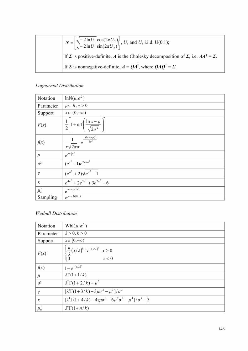
146

−−

=)2sin(ln2

)2cos(ln2

21

21

UπU

UπUN , U1 and U2 i.i.d. U(0,1);

If Σ is positive-definite, A is the Cholesky decomposition of Σ, i.e. AAT = Σ.

If Σ is nonnegative-definite, A = QΛ1

2, where QΛQT = Σ.

Lognormal Distribution

Notation ),lnN( 2σµ

Parameter 0 , >∈ σRµ

Support ),0( +∞∈x

F(x)

−+

22

lnerf1

2

1

σ

µx

f(x) 2

2

2

)(ln

2

1σ

µx

eσπx

−−

µ 2

2

1 σµe

+

σ2 22 2)1( σµσ ee +−

γ 1)2(22

−+ σσ ee

κ 632222 234 −++ σσσ eee

µ'n

22

2

1 σnµne

+

Sampling )1,0N(σµe +

Weibull Distribution

Notation ),Wbl( 2σµ

Parameter 0 ,0 >> kλ

Support ),0[ +∞∈x

F(x) ( ) ( )

<

≥−−

0 0

0 1

x

xeλxλ

k kλxk

f(x) ( )kλxe−−1

µ )/11(Γ kλ +

σ2 22 )/21(Γ µkλ −+

γ 3323 /]3)/31(Γ[ σµµσkλ −−+

κ 3/]64)/41(Γ[ 442234 −−−−+ σµσµγµσkλ

µ'n )/1(Γ knλn +

147

Sampling k

λ)1,0lnU(

1−

4.2 Discrete Probability Distribution

Bernoulli Distribution

Notation )Ber( p

Parameter 10 << p

Support 1,0=x

F(x)

≥<≤−

<

1 110 1

0 0

xxp

x

f(x)

==−

1 0 1

xpxp

µ p

σ2 )1( pp −

γ )1(

21

pp

p

−

−

κ 6)1(

1−

− pp

µ'n p

Sampling

−>−≤

pp

1(0,1)U 11(0,1)U 0

Binomial Distribution

Notation ),Bin( pN

Parameter 10,0 <<∈ pNN

Support ,,1,0 Nx ⋯=

F(x)

∑=

−−

=+−−

x

i

iNi ppiN

xxNp0

)1()1,;1(Ι

f(x) xNx pp

xN −−

)1(

µ Np

σ2 )1( pNp −

γ )1(

21

pNp

p

−

−

148

κ NpNp

6

)1(

1−

−

κn

≥−=

=− 2 )1( 1

1

ndp

κdppκ

Npκ

nn

Sampling

−>−=≤<−

≤

)1()1,0U( 1,,2,1),()1,0U()1(

)0()1,0U( 0

NFNNiiFiFi

F⋯

149

LIST OF PUBLICATIONS

[1] G. Li and X.-P. Zhang, “Modelling of Plug-in Hybrid Electric Vehicle Charging Demand

in Probabilistic Power Flow Calculations,” IEEE Transactions on Smart Grid, vol. 3, no.

1, pp. 492-499, Mar. 2012.

[2] G. Li and X.-P. Zhang, “Stochastic Optimal Power Flow Approach Considering

Correlated Probabilistic Load and Wind Farm Generation,” in Proceedings of 2011 IET

Conference on Reliability of Transmission and Distribution Networks, London, UK, vol.

CP580, pp. 3A1-3A7, Nov. 22-24 2011.

[3] G. Li, X.-P. Zhang, and X. Wang, “Accelerated Newton-Raphson Power Flow,”

European Transactions on Electrical Power, vol. 22, no. 4, pages 504–517, May 2012

[4] G. Li, X.-P. Zhang, “Comparison between Two Probabilistic Load Flow Methods for

Reliability Assessment,” in Proceedings of 2009 IEEE Power and Energy Society

General Meeting, Calgary, Alberta, AB, Canada, pp. 1-7, Jul. 26-30 2009.

[5] Z. Bie, H. Liu, G. Li, et al., “Voltage Fluctuation Analysis of a Power System with Wind

Farms Integrated by Probabilistic Load Flow,” Journal of Xi’an Jiaotong University, vol.

42, no. 12, pp. 1500-1505, Dec. 2008.

[6] Z. Bie, G. Li, H. Liu, et al., “Studies on Voltage Fluctuation in the Integration of Wind

Power Plants Using Probabilistic Load Flow,” in Proceedings of 2008 IEEE Power and

Energy Society General Meeting, Pittsburgh, PA, USA, pp. 1-7, Jul. 20-24 2008.

150

LIST OF REFERENCES

[1] S. Newman, The Final Energy Crisis, 2nd Edition. London: Pluto Press, 2008.

[2] H. Michael and K. Snorre, “Depletion of Fossil Fuels and the Impacts of Global

Warming,” Resource and Energy Economics, vol. 18, no. 2, pp. 115-136, Jun. 1996.

[3] European Wind Energy Association, Wind Energy - The Facts. London: Earthscan,

2009.

[4] E. Ungar and K. Fell, “Plug in, Turn on, and Load up,” IEEE Power and Energy

Magazine, vol. 8, no. 3, pp. 30-35, May 2010.

[5] D. Seligsohn, R. Heilmayr, X. Tan, and L. Weischer, China, the United States, and the

Climate Change Challenge, World Resources Institute, Tech. Report, Oct. 2009,

[Online]. Available: http://www.wri.org/publication/china-united-states-climate-change

-challenge/.

[6] S. M. Amin and B. F. Wollenberg, “Toward a Smart Grid: Power Delivery of the 21st

Century,” IEEE Power and Energy Magazine, vol. 3, no. 5, pp. 34-41, Sept. 2005.

[7] X. Zhou, “Present Situation and Trend of Energy Consumption in Traffic and

Transportation Industry,” Sino-Global Energy, vol. 15, no. 7, pp. 9-18, Jul. 2010.

[8] R. D. Richardson and G. M. Mcnerney, “Wind Energy Systems,”, Proceedings of the

IEEE, vol. 81, no. 3, pp. 378-389, Mar. 1993.

[9] P. Musgrove, “Wind Energy,” Cambridge: Cambridge University Press, 2009.

[10] World Wind Energy Association Head Office, World Wind Energy Half-Year Report

2011, World Wind Energy Association, Tech. Report, Aug. 2011.

[11] RenewableUK, “UK Wind Energy Database Statistics,” March 2012, [Online].

Available: http://www.bwea.com/statistics/.

[12] A. Smith, “Two Terawatts Average Power Output: The UK Offshore Wind Resource,”

Sept. 2010, [Online]. Available: http://www.claverton-energy.com/two-terawatts-avera

ge-power-output-the-uk-offshore-wind-resource.html/.

[13] J. Oswald, M. Raine, and H. Ashraf-Ball, “Will British Weather Provide Reliable

Electricity?,” Energy Policy, vol. 36, no. 8, pp. 2312-2325, Jun. 2008.

[14] M. Etezadi-Amoli, K. Choma, and J. Stefani, “Rapid-Charge Electric-Vehicle

Stations,” IEEE Transactions on Power Delivery, vol. 25, no. 3, pp. 1883-1887, Jul.

2010.

151

[15] European Commission, “Reducing Emissions from Transport,” Jan. 2011, [Online].

Available: http://ec.europa.eu/clima/policies/transport/index_en.htm/.

[16] A. K. Srivastava, B. Annabathina, and S. Kamalasadan, “The Challenges and Policy

Options for Integrating Plug-in Hybrid Electric Vehicle into the Electric Grid,” The

Electricity Journal, vol. 23, no. 3, pp. 83-91, Mar. 2010.

[17] D. Sperling, and G. Deborah, Two Billion Cars: Driving toward Sustainability. New

York: Oxford University Press, 2009.

[18] D. B. Sandalow, Plug-In Electric Vehicles: What Role for Washington?. Washington:

The Brookings Institution, 2009.

[19] C. Woodyard, “Obama Pushes Electric Cars, Battery Power This Week,” USA Today,

Jul. 2010.

[20] K. Bradsher, “In China, Power in Nascent Electric Car Industry,” New York Times,

Dec. 2011.

[21] C. Schweinsberg, “U.S. Hybrid Sales Hit 2 Million Mark,” WardsAuto, Jun. 2011.

[22] A. Shimbun, “Hybrids Now 16% of Market in Japan as Prius Wins Annual Sales

Crown Again,” Integrity Exports, Apr. 2012.

[23] A. Vaughan, “UK Government Launches £5,000 Electric Car Grant Scheme,” Jan.

2011, [Online]. Available: http://www.guardian.co.uk/environment/2011/jan/01/electric

-car-grant-uk/.

[24] D. Vince, “Our Electric Highway Will Kick Start Britain's Green Car Revolution,” Jul.

2011, [Online]. Available: http://www.guardian.co.uk/environment/2011/jul/27/ electric

-motorway-green-cars/.

[25] Society of Motor Manufacturers and Traders, “December 2011 – EV and AFV

Registrations,” Jan. 2012, [Online]. Available: http://www.smmt.co.uk/2012/01/

december-2011-%E2%80%93-ev-and-afv-registrations/.

[26] J. Siegel, “Electric Vehicle Market Will Grow 20 Percent Annually,” Dec. 2011,

[Online]. Available: http://www.greenchipstocks.com/articles/electric-vehicle-market-

growth/1467/.

[27] Y. Wu, “Research on Reliability Evaluation and Expansion Planning of Power System

including Wind Farms,” Ph.D. dissertation, School of Electric Engineering, Hefei

University of Technology, Hefei, Anhui, China, 2006.

152

[28] Z. Hu, Y. Song, Z. Xu, et al., “Impacts and Utilization of Electric Vehicles into Power

Systems,” Proceedings of the CSEE, vol. 32, no. 4, pp. 1-11, Feb. 2012.

[29] C. Gao and L. Zhang, “A Survey of Influence of Electrics Vehicle Charging on Power

Grid,” Power System Technology, vol. 35, no. 2, pp. 127-131, Feb. 2011.

[30] W. F. Tinney and C. E. Hart, “Power Flow Solution by Newton's Method,” IEEE

Transactions on Power Apparatus and Systems, vol. 86, no. 11, pp. 1449-1460, Nov.

1967.

[31] E. Moore K. Ganesan, W. J. Vetter, “On Convergence of Newton's Method for Load

Flow Problems,” International Journal for Numerical Methods in Engineering, vol. 7,

no.3, pp. 325-336, Jul. 1973.

[32] B. Stott, “Review of Load-Flow Calculation Methods,” Proceedings of IEEE, vol.62,

no. 7, pp. 916-929, Jul. 1974.

[33] B. Scott and O. Alsac, “Fast Decoupled Load Flow,” IEEE Transactions on Power

Apparatus and Systems, vol. 93, no. 3, pp. 859-869, May 1974.

[34] V. Ajjarapu and C. Christy, “The Continuation Power Flow: A Tool for Steady-State

Voltage Stability Analysis,” IEEE Transactions on Power Systems, vol. 7, no. 1, pp.

416-423, Feb. 1992.

[35] S. Iwamoto and Y. Tamura, “A Load Flow Method for Ill-Conditioned Power

Systems,” IEEE Trans. on Power Apparatus and Systems, vol. 100, no.4, pp. 1736-

1743, Apr. 1981.

[36] V. M. da Costa, N. Martins, and J. L. R. Pereira, “Developments in the Newton

Raphson Power Flow Formulation Based on Current Injections,” IEEE Transactions on

Power Systems, vol. 14, no. 4, pp. 1320-1326, Nov. 1999.

[37] V. M. da Costa, J. L. R. Pereira, and N. Martins, “An Augmented Newton-Raphson

Power Flow Formulation Based on Current Injections,” International Journal of

Electrical Power & Energy Systems, vol. 23, no. 4, pp. 305-312, May 2001.

[38] C. A. Ferreira and V. M. da Costa, “A Second Order Power Flow Based on Current

Injection Equations,” International Journal of Electrical Power & Energy Systems, vol.

27, no. 4, pp. 254-263, May 2005.

[39] T. Kulworawanichpong, “Simplified Newton-Raphson Power-Flow Solution Method,”

International Journal of Electrical Power & Energy Systems, vol. 32, no. 6, pp. 551-

558, Jul. 2010.

153

[40] V. M. da Costa and A. Rosa, “A Comparative Analysis of Different Power Flow

Methodologies," in Proceedings of 2008 IEEE/PES Transmission and Distribution

Conference and Exposition: Latin America, Bogota, Colombia, pp.1-7, Aug. 13-15

2008.

[41] F. Milano, “Continuous Newton’s Method for Power Flow Analysis,” IEEE

Transactions on Power Systems, vol. 24, no. 1, pp. 50-57, Feb. 2009.

[42] S. Iwamoto and Y. Tamura, “A Load Flow Calculation Method for Ill-Conditioned

Power Systems,” IEEE Transactions on Power Apparatus and Systems, vol. 100, no. 4,

pp.1736-1743, Apr. 1981.

[43] L. M. C. Braz, C. A. Castro, and C. A. F. Murati, “A Critical Evaluation of Step Size

Optimization Based Load Flow Methods,” IEEE Transactions on Power Systems, vol.

15, no. 1, pp.202-207, Feb. 2000.

[44] J. E. Tate and T. J. Overbye, “A Comparison of the Optimal Multiplier in Polar and

Rectangular Coordinates,” IEEE Transactions on Power Systems, vol. 20, no. 4, pp.

1667- 1674, Nov. 2005.

[45] R. S. Salgado and A. F. Zeitune, “Power Flow Solutions through Tensor Methods,”

IET Generation, Transmission & Distribution, vol. 3, no. 5, pp. 413-424, May 2009.

[46] A. C. Z. de Souza, C. B. Rosa, I. L. Lopes, and et al., “Non-Iterative Load-Flow

Method as A Tool for Voltage Stability Studies,” IET Generation Transmission &

Distribution, vol. 1, no. 3, pp. 499-505, May 2007.

[47] A. Karami, and M. S. Mohammadi, “Radial Basis Function Neural Network For Power

System Load-Flow,” International Journal of Electrical Power & Energy Systems, vol.

30, no. 1, pp. 60-66, Jan. 2008.

[48] P. ACHARJEE and S. K. GOSWAMI, “Chaotic Particle Swarm Optimization Based

Robust Load Flow,” International Journal of Electrical Power & Energy Systems, vol.

32, no. 2, pp. 141-146, Feb. 2008.

[49] A. Semlyen and F. de Leon, “Quasi-Newton Power Flow Using Partial Jacobian

Updates,” , IEEE Transactions on Power Systems, vol. 16, no. 3, pp.332-339, Aug.

2001.

[50] G. Radman and J. Shultz, “An Effective Calculation Procedure for the Newton-

Raphson Power Flow Analysis,” in Proceedings of 7th ISATED International Multi-

154

Conference on Power and Energy Systems, Calgary, Canada, pp. 149-153, Feb. 24-26

2003.

[51] P. J. Lagace, M. H. Vuong and I. Kamwa, “Improving Power Flow Convergence by

Newton Raphson with a Levenberg-Marquardt Method,” in Proceedings of 2008 IEEE

Power and Energy Society General Meeting, Pittsburgh, PA, USA, pp.1-6, 20-24 Jul.

2008.

[52] K. L. Lo and Z. J. Meng, “Newton-Like Method for Line Outage Simulation,” IEE

Proceedings of Generation, Transmission and Distribution, vol. 151, no. 2, pp. 225-231,

Mar. 2004.

[53] N. S. Krejić and Z. Luźanin, “Newton-Like Method with Modification of the Right-

Hand-Side Vector,” Mathematics of Computation, vol. 71, no. 237, pp. 237-250, Jan.

2002.

[54] R. S. Dembo, S. C. Eisenstat, and T. Steihaug, “Inexact Newton Methods,” SIAM

Journal on Numerical Analysis, vol. 19, no. 2, pp. 400-408, Apr. 1982.

[55] S. C. Eisenstat and H. F. Walker, “Choosing the Forcing Terms in an Inexact Newton

Method,” SIAM Journal on Scientific Computing, vol. 17, no. 1, pp. 16-32, Jan. 1996.

[56] D. Herceg, N. S. Krejić, and Z. Luźanin, “Quasi-Newton’s Method with Correction,”

Novi Sad Journal of Mathematics, vol. 26, no. 1, pp. 115-127, Jan. 1996

[57] G. Zhou and L. Qi, “On the Convergence of an Inexact Newton-Type Method,”

Operations Research Letters, vol. 34, no. 6, pp. 647-652, Nov. 2006.

[58] C. Xu, N. Wang, and M. Wang, “Study of Accelerated Newton-Like Method with

Modification of the Right-Hand-Side Vector,” Journal of Huazhong University of

Science and Technology (Nature Science Edition), vol. 34, no. 4, pp. 119-121, Apr.

2006.

[59] I. K. Argyros, S. Hilout, “Inexact Newton-type Methods,” Journal of Complexity, vol.

26, no. 6, pp. 577-590, Dec. 2010.

[60] A. K. Srivastava, B. Annabathina, and S. Kamalasadan, “The Challenges and Policy

Options for Integrating Plug-in Hybrid Electric Vehicle into the Electric Grid,” The

Electricity Journal, vol. 23, no. 3, pp. 83-91, Apr. 2010. [61] T. H. Bradleya and A. A. Frankb, “Design, Demonstrations and Sustainability Impact

Assessments for Plug-In Hybrid Electric Vehicle,” Renewable and Sustainable Energy

Reviews, vol. 13, no. 1, pp. 115-128, Jan. 2009.

155

[62] S. S. Williamson, “Electric Drive Train Efficiency Analysis Based on Varied Energy

Storage System Usage for Plug-In Hybrid Electric Vehicle,” in Proceedings of 2007

IEEE Power Electronics Specialists Conference, Orlando, FL, USA, pp.1515-1520, Jul.

17-21 2007.

[63] G. T. Heydt, “The Impact of Electric Vehicle Deployment on Load Management

Strategies,” IEEE Transactions on Power Apparatus & System, vol. 1, no. 144, pp.

1253-1259, May 1983.

[64] A. Heider and H. J. Haubrich, “Impact of Wide-Scale EV Charging on the Power

Supply Network,” in Proceedings of IEE Colloquium on Electric Vehicles: A

Technology Roadmap for the Future, London, UK, vol. 6, no. 262, pp. 1-4, May 5

1998.

[65] K. Schneider, C. Gerkensmeyer, M. Kintner-Meyer, and M. Fletcher, “Impact

Assessment of Plug-In Hybrid Electric Vehicles on Pacific Northwest Distribution

Systems,” in Proceedings of 2008 IEEE Power and Energy Society General Meeting,

Pittsburgh, PA, USA, pp. 1-6, Jul. 20-24 2008.

[66] K. Mets, T. Verschueren, W. Haerick, et al., “Optimizing Smart Energy Control

Strategies for Plug-In Hybrid Electric Vehicle Charging,” in Proceedings of 12th

IEEE/IFIP Network Operations and Management Symposium Workshops, Osaka, Japan,

pp. 293-299, Apr. 19-23 2010.

[67] N. Rotering and M. Ilic, “Optimal Charge Control of Plug-In Hybrid Electric Vehicles

in Deregulated Electricity Markets,” IEEE Transactions on Power Systems, vol. 26, no.

3, pp. 1021-1029, Aug. 2011.

[68] W. Kempton and J. Tomic, “Vehicle-to-Grid Power Fundamentals: Calculating

Capacity and Net Revenue,” Journal of Power Sources, vol. 144, no. 1, pp. 268-279,

Jun. 2005.

[69] W. Kempton and J. Tomic, “Vehicle-to-Grid Power Implementation: From Stabilizing

the Grid to Supporting Large-Scale Renewable Energy,” Journal of Power Sources, vol.

144, no. 1, pp. 280-294, Jun. 2005.

[70] H. Turton and F. Moura, “Vehicle-to-Grid Systems for Sustainable Development: An

Integrated Energy Analysis,” Technological Forecasting and Social Change, vol. 75,

no. 8, pp. 1091-1108, Oct. 2008.

156

[71] C. Guille and G. Gross, “A Conceptual Framework for the Vehicle-to-Grid (V2G)

Implementation,” Energy Policy, vol. 37, no. 11, pp. 4379-4390, Nov. 2009.

[72] W. Kempton and J. Tomic, “Vehicle-to-Grid Power Fundamentals: Calculating

Capacity and Net Revenue,” Journal of Power Sources, vol. 144, no. 1, pp. 268-279,

Jun. 2005.

[73] W. Kempton and J. Tomic, “Vehicle-to-Grid Power Implementation: From Stabilizing

the Grid to Supporting Large-Scale Renewable Energy,” Journal of Power Sources, vol.

144, no. 1, pp. 280-294, Jun. 2005.

[74] M. Etezadi-Amoli, K. Choma, and J. Stefani, “Rapid-Charge Electric-Vehicle

Stations,” IEEE Transactions on Power Delivery, vol. 25, no. 3, pp. 1883-1887, Jul.

2010.

[75] K. Clement-Nyns, E. Haesen, and J. Driesen, “The Impact of Charging Plug-In Hybrid

Electric Vehicles on a Residential Distribution Grid”, IEEE Transactions on Power

Systems, vol. 25, no. 1, pp. 371-380, Feb. 2010.

[76] U. N. Bhat, An Introduction to Queueing Theory: Modeling and Analysis in

Applications. New York: Birkhäuser Boston & Springer Science, 2008.

[77] R. Garcia-Valle, and J. G. Vlachogiannis, “Electric Vehicle Demand Model for Load

Flow Studies”, Electric Power Components & Systems, vol. 37, no. 5, pp. 577-582,

May 2009.

[78] J. G. Vlachogiannis, “Probabilistic Constrained Load Flow Considering Integration of

Wind Power Generation and Electric Vehicles”, IEEE Transactions on Power Systems,

vol. 24, no. 4, pp. 1808-1817, Nov. 2009.

[79] S. Meliopoulos, Power System Level Impacts of Plug-In Hybrid Vehicles, Power

Systems Engineering Research Center (PSERC), Tech. Report, Oct. 2009, [Online].

Available: www.pserc.wisc.edu/research/public_reports/td.aspx/.

[80] B. Borkowska, “Probabilistic Load Flow,” IEEE Transactions on Power Apparatus and

Systems, vol. 93, pp. 752-759, May 1974.

[81] A. M. L. d. Silva and V. L. Arienti, “Probabilistic Load Flow by a Multi-linear

Simulation Algorithm,” IEE Proceedings of Generation Transmission and Distribution,

vol. 137, pp. 276-282, Jul. 1990.

[82] R. Billinton and W. Li, Reliability Assessment of Electric Power Systems Using Monte

Carlo Methods. New York: Plenum, 1994.

157

[83] P. Jirutitijaroen and C. Singh, “Comparison of Simulation Methods for Power System

Reliability Indexes and Their Distributions,” IEEE Transactions on Power Systems, vol.

23, pp. 486-493, Apr. 2008.

[84] R. N. Allan, B. Borkowska, and C. H. Grigg, “Probabilistic Analysis of Power Flows,”

Proceedings of the Institute of Electrical Engineers, vol. 121, no 12, pp. 1551-1556,

Dec. 1974.

[85] R. N. Allan and M. R. G. Al-Shakarchi, “Probabilistic Techniques in A.C. Load-Flow

Analysis,” Proceedings of the Institute of Electrical Engineers, vol. 124, pp. 154-160,

Feb. 1977.

[86] R. N. Allan and M. R. G. Al-Shakarchi, “Linear Dependence between Nodal Powers in

Probabilistic A.C. Load Flow”, Proceedings of IEE, vol. 124, no. 6, pp. 529-534, Jun.

1977.

[87] R. N. Allan, A. M. L. da Silva, and R. C. Burchett, “Evaluation Methods and Accuracy

in Probabilistic Load Flow Solutions,” IEEE Transactions on Power Apparatus and

Systems, vol. 100, pp. 2539-2546, May 1981.

[88] R. N. Allan and A. M. L. Dasilva, “Probabilistic Load Flow Using Multi-

linearizations,” IEE Proceedings of Generation Transmission and Distribution, vol. 128,

no. 5, pp. 280-287, May 1981.

[89] A. M. L. d. Silva, V. L. Arienti, and R. N. Allan, “Probabilistic Load Flow Considering

Dependence between Input Nodal Powers,” IEEE Transactions on Power Apparatus

and Systems, vol. 103, pp. 1524-1530, Jun. 1984.

[90] M. Brucoli and F. Torelli, “Quadratic Probabilistic Load Flow with Linearly Modeled

Dispatch,” International Journal of Electrical Power & Energy Systems, vol. 7, pp.

138-146, Jul. 1985.

[91] A. M. L. Dasilva, R. N. Allan, S. M. Soares, and V. L. Arienti, “Probabilistic Load

Flow Considering Network Outages,” IEE Proceedings of Generation Transmission

and Distribution, vol. 132, pp. 139-145, May 1985.

[92] L. A. Sanabria and T. S. Dillon, “Stochastic Power Flow Using Cumulants and Von

Mises Functions,” International Journal of Electrical Power & Energy Systems, vol. 8,

pp. 47-60, Jan. 1986.

[93] S. Patra and R. B. Misra, “Probabilistic Load Flow Solution Using Method of

Moments,” in Proceedings of 2nd International Conference on Advances in Power

158

System Control, Operation & Management, Hong Kong, vol. 1 and 2, pp. 922-934 &

991, Dec. 7-10 1993.

[94] P. Zhang and S. T. Lee, “Probabilistic Load Flow Computation Using the Method of

Combined Cumulants and Gram-Charlier Expansion,” IEEE Transactions on Power

Systems, vol. 19, pp. 676-682, Feb. 2004.

[95] Z. Hu and X. Wang, “A Probabilistic Load Flow Method Considering Branch

Outages,” IEEE Transactions on Power Systems, vol. 21, pp. 507-514, May 2006.

[96] M. Lu, Z. Y. Dong, and T. K. Saha, “A Probabilistic Load Flow Method Considering

Transmission Network Contingency,” in Proceedings of 2007 IEEE Power Engineering

Society General Meeting, Tampa, FL, USA, pp. 1-6, Jun. 24-28 2007.

[97] J. Usaola, “Probabilistic Load Flow with Wind Production Uncertainty Using

Cumulants and Cornish-Fisher Expansion,” International Journal of Electrical Power

& Energy Systems, vol. 31, no. 9, pp. 474-481, Sept. 2009.

[98] J. Usaola, “Probabilistic Load Flow with Correlated Wind Power Injections,” Electric

Power Systems Research, vol. 80, no. 5, pp. 528-536, May 2010.

[99] F. J. Ruiz-Rodriguez, J. C. Hernández, and F. Jurado, “Probabilistic Load Flow for

Photovoltaic Distributed Generation Using the Cornish-Fisher Expansion,” Electric

Power Systems Research, vol. 89, no. 8, pp. 129-138, Aug. 2012.

[100] C.-L. Su, “Probabilistic Load-Flow Computation Using Point Estimate Method,” IEEE

Transactions on Power Systems, vol. 20, pp. 1843-1851, Nov. 2005.

[101] J. M. Morales and J. Perez-Ruiz, “Point Estimate Schemes to Solve the Probabilistic

Power Flow,” IEEE Transactions on Power Systems, vol. 22, pp. 1594-1601, Nov.

2007.

[102] J. M. Morales, L. Baringo, A. J. Conejo, et al., “Probabilistic Power Flow with

Correlated Wind Sources,” IET Generation, Transmission & Distribution, vol. 4, no. 5,

pp. 641-651, May 2010.

[103] M. T. Schilling, A. M. Leite da Silva, R. Billinton, et al., “Bibliography on Power

System Probabilistic Analysis (1962-88),” IEEE Transactions on Power Systems, vol. 5,

pp. 1-11, 1990.

[104] P. Chen, Z. Chen, and B. Bak-Jensen, “Probabilistic Load Flow: A Review,” in

Proceedings of 3rd International Conference on Electric Utility Deregulation and

159

Restructuring and Power Technologies, Nanjing, Jiangsu, China, pp.1586-1591, Apr. 6-

9 2008.

[105] J. Carpentier, “Optimal Power Flows,” International Journal of Electrical Power &

Energy Systems, vol.1, no. 1, pp. 3-15, Apr. 1979.

[106] Y. Taiyou and R. H. Lasseter, “Stochastic Optimal Power Flow: Formulation and

Solution,” in Proceedings of 2000 IEEE Power Engineering Society Summer Meeting,

Seattle, WA, USA, vol. 1, pp. 237-242, 2000.

[107] A. Schellenberg, “Probabilstic and Stochastic Optimal Power Flow,” Ph.D. dissertation,

Department of Electric and Computer Engineering, University of Calgary, Alberta,

Canada, 2006.

[108] G. L. Viviani and G. T. Heydt, “Stochastic Optimal Energy Dispatch,” IEEE

Transactions on Power Apparatus and Systems, vol. 100, no. 07, pp. 3221-3227, Jul.

1981.

[109] M. Madrigal, K. Ponnambalam, and V. H. Quintana, “Probabilistic Optimal Power

Flow,” in Proceedings of 1998 IEEE Canadian Conference on Electrical and Computer

Engineering, Toronto, Canada, pp. 385-388, May 24-28 1998.

[110] A. Schellenberg, W. Rosehart, and J. Aguado, “Cumulant Based Probabilistic Optimal

Power Flow (P-OPF),” in Proceedings of 2004 International Conference on

Probabilistic Methods Applied to Power Systems, Ames, LA, USA, pp. 506-511, Sept.

12-16 2004.

[111] A. Schellenberg, W. Rosehart, and J. Aguado, “Cumulant-Based Probabilistic Optimal

Power Flow (P-OPF) with Gaussian and Gamma Distributions,” IEEE Transactions on

Power Systems, vol. 20, no. 2, pp. 773-781, May 2005.

[112] G. Verbic, and C. A. Canizares, “Probabilistic Optimal Power Flow in Electricity

Markets Based on a Two-Point Estimate Method,” IEEE Transactions on Power

Systems, vol. 21, no. 4, pp. 1883-1893, Nov. 2006.

[113] G. Verbic, A. Schellenberg, W. Rosehart, et al., “Probabilistic Optimal Power Flow

Applications to Electricity Markets,” in Proceedings of 2006 International Conference

on Probabilistic Methods Applied to Power Systems, Stockholm, Sweden, pp. 348-353

& 1244, Jun. 11-15 2006.

160

[114] X. Li, Y. Z. Li, and S. H. Zhang, “Analysis of Probabilistic Optimal Power Flow

Taking Account of the Variation of Load Power,” IEEE Transactions on Power

Systems, vol. 23, no. 3, pp. 992-999, Aug. 2008.

[115] M. E. El-Hawary, and G. A. N. Mbamalu, “Stochastic Optimal Load Flow Using a

Combined Quasi-Newton and Conjugate Gradient Technique,” International Journal of

Electrical Power & Energy Systems, vol.11, no. 2, pp. 85-93, Apr. 1989.

[116] Z. Hu and X. Wang, “Stochastic Optimal Power Flow Approach Considering Load

Probabilistic Distributions,” Automation of Electric Power Systems, vol. 31, no. 16, pp.

14-17 & 44, Nov. 2007.

[117] Z. Hu, X. Wang, and G. Taylor, “Stochastic Optimal Reactive Power Dispatch:

Formulation and Solution Method,” International Journal of Electrical Power &

Energy Systems, vol. 32, no. 6, pp. 615-621, Jul. 2010.

[118] H. Zhang and P. Li, “Probabilistic Analysis for Optimal Power Flow under

Uncertainty,” IET Generation, Transmission & Distribution, vol. 4, no. 5, pp. 553-561,

May 2010.

[119] Y. Yuan, Q. Li, and W. Wang, “Optimal Operation Strategy of Energy Storage Unit in

Wind Power Integration Based on Stochastic Programming,” IET Renewable Power

Generation, vol. 5, no.2, pp. 194-201, May 2011.

[120] B. Liu, Theory and Practice of Uncertain Programming, 2nd Edition. Berlin: Springer

Press, 2009.

[121] P. F. Correia, J. M. Ferreira de Jesus, “Simulation of Correlated Wind Speed and Power

Variates in Wind Parks,” Electric Power Systems Research, vol. 80, no. 5, pp. 592-598,

May 2010.

[122] W. H. Press, S. A. Teukolsky, W. T. Vetterling, et al., Numerical Recipes: The Art of

Scientific Computing, Third Edition. Cambridge: Cambridge University Press.

[123] T. A. Davis, Direct Methods for Sparse Linear Systems - Fundamentals of Algorithms.

Philadelphia: Society for Industrial and Applied Mathematics, 2006.

[124] J. E. Dennis Jr. and R. B. Schnabel, Numerical Methods for Unconstrained

Optimization and Nonlinear Equations. Philadelphia: Society for Industrial

Mathematics, 1983.

[125] G. A. Korn and T. M. Korn, Mathematical Handbook for Scientists and Engineers.

New York: Dover Publications, 2000.

161

[126] S. M. Chan, and V. Brandwajn, “Partial Matrix Refactorization,” IEEE Transactions

on Power Systems, vol. 1, no. 1, pp. 193-200, Jan. 1986.

[127] Y. Zhang, and W. F. Tinney, “Partial Refactorization with Unrestricted Topology

Changes,” IEEE Transactions on Power Systems, vol. 10, no. 3, pp. 1361-1368, Jul.

1995.

[128] J. Walter, M. Koch, G. Winkler, and D Bellot, “Basic Linear Algebra Library,” Nov.

2010, [Online]. Available: http://www.boost.org/libs/numeric/.

[129] T. A. Davis, and E. P. Natarajan, “KLU: Sparse LU Factorization,” May 2007,

[Online]. Available: http://www.cise.ufl.edu/research/sparse/klu/.

[130] B. Dawes, “Boost Timer Library,” Oct. 2011, [Online]. Available: www.boost.org/

doc/libs/release/libs/timer/.

[131] H. Fischer, A History of the Central Limit Theorem: from Classical to Modern

Probability Theory. New York: Springer, 2010.

[132] R. V. Hogg, J. W. McKean, and A. T. Craig, Introduction to Mathematical Statistics,

6th Edition. Upper Saddle River, New Jersey: Prentice Hall, 2004.

[133] N. L. Johnson, A. W. Kemp, and S. Kotz, Univariate Discrete Distributions, 3rd

Edition. Hoboken, NJ: Wiley-Interscience, 2005.

[134] W. T. Pennell and A. H. Miller, “Procedures for Modeling Wind Turbine Performance

from Site Wind Data,” in Proceedings of 5th Annual Energy-Sources Technology

Conference and Exhibition, New Orleans, LA, USA, 82-PET-7, Mar. 7-10 1982.

[135] G. J. Bowden, P. R. Barker, V. O. Shestopal, and J. W. Twidell, “The Weibull

Distribution Function and Wind Power Statistics,” Wind Energy, vol. 7, no. 2, pp. 85-98,

Apr. 1983.

[136] R. B. Corotis, A. B. Sigl, and J. Klein, “Probability Models of Wind Velocity

Magnitude and Persistence,” Solar Energy, vol. 20, no. 6, pp. 483-493, Jun. 1978.

[137] S. H. Jangamshetti and V. G. Rau, “Site Matching of Wind Turbine Generators: A

Case Study,” IEEE Transactions on Energy Conversion, vol. 14, no. 4, pp. 1537-1543,

Dec. 1999.

[138] A. E. Feijoo, J. Cidras, and J. L. G. Dornelas, “Wind Speed Simulation in Wind Farms

for Steady-State Security Assessment of Electrical Power Systems”, IEEE Transactions

on Energy Conversion, vol.14, no. 4, pp. 1582-1588, Dec. 1999.

162

[139] A. Garcia, J. L. Torres, E. Prieto, and A. de Francisco, “Fitting Wind Speed

Distributions: A Case Study,” Solar Energy, vol. 62, no. 2, pp. 139-144, Feb. 1998.

[140] A. Balouktsis, D. Chassapis, and T. D. Karapantsios, “A Nomogram Method for

Estimating the Energy Produced by Wind Turbine Generators,” Solar Energy, vol. 72,

no. 3, pp. 251-259, Mar. 2002.

[141] Y. Muluge and F. Drake, “Assessment of Solar and Wind Energy Resources in

Ethiopia II: Wind Energy,” Solar Energy, vol. 57, no. 4, pp. 323-334, Oct. 1996.

[142] S. H. Jangamshetti and V. Rau, “Optimum Siting of Wind Turbine Generators,” IEEE

Transactions on Energy Conversion, vol. 16, no. 1, pp. 8-13, Mar. 2001.

[143] A. Van den Bos, Parameter Estimation for Scientists and Engineers. Hoboken, NJ:

Wiley-Interscience, 2007.

[144] L. Ranch, New Mexico Wind Resource Assessment, Sandia National Laboratories,

Tech. Report, Feb. 2003, Online. Available: http://www.sandia.gov/wind/other/

LeeRanchData-2002.pdf/.

[145] G. N. Kariniotakis and P. Pinson, “Uncertainty of Short-term Wind Power Forecasts: A

Methodology for On-line Assessment,” in Proceedings of 2004 International

Conference on Probabilistic Methods Applied to Power Systems, Ames, IA, USA,

pp.729-736, Sept. 16 2004.

[146] S. F. Castro and R. N. Allan, “Generation Availability Assessment of Wind Farms,”

Proceedings of IEE Generation, Transmission and Distribution, vol.143, no.5, pp.507-

518, Sept. 1996.

[147] X. Zhang; W. Wang, “Wind Farm and Wake Effect Modeling for Simulation of a

Studied Power System,” in Proceedings of 2009 Power Systems Conference and

Exposition, Seattle, WA, USA, pp.1-6, Mar. 15-18 2009.

[148] A. Marinopoulos, J. Pan, M. Zarghami, et al., “Investigating the Impact of Wake Effect

on Wind Farm Aggregation,” in Proceedings of 2011 IEEE Trondheim PowerTech,

Trondheim, Norway, pp.1-5, Jun. 19-23 2011.

[149] J. K. Sethi, D. Deb, M. Malakar, “Modeling of a Wind Turbine Farm in Presence of

Wake Interactions,” in Proceedings of 2011 International Conference on Energy,

Automation, and Signal, Bhubaneswar, India, pp.1-6, Dec. 28-30 2011.

[150] A. Fabbri, T. GomezSanRoman, J. RivierAbbad, et al., “Assessment of the Cost

Associated with Wind Generation Prediction Errors in a Liberalized Electricity

163

Market,” IEEE Transactions on Power Systems, vol.20, no.3, pp. 1440-1446, Aug.

2005.

[151] M. Lange, “On the Uncertainty of Wind Power Predictions - Analysis of the Forecast

Accuracy and Statistical Distribution of Errors,” Journal of Solar Energy Engineering,

vol. 127, no. 2, pp. 177-185, May 2005.

[152] J. Usaola and J. Angarita, “Bidding Wind Energy under Uncertainty,” in Proceedings

of 2007 International Conference on Clean Electrical Power, Capri, Italy, pp.754-759,

May 21-23 2007.

[153] H. Bludszuweit, J. A. Dominguez-Navarro, and A. Llombart, “Statistical Analysis of

Wind Power Forecast Error”, IEEE Transactions on Power Systems, vol. 23, no. 3, pp.

983-991, Aug. 2008.

[154] K. T. Chau and Y. S. Wong, “Overview of Power Management in Hybrid Electric

Vehicles”, Energy Conversion and Management, vol. 43, no. 15, pp. 1953-1968, Oct.

2002.

[155] L. Sanna, “Driving the Solution the Plug-In Hybrid Electric Vehicle”, EPRI Journal,

pp. 8-17, Sept. 2005.

[156] S. M. Ross, Stochastic Processes, 2nd Edition. New York: Wiley, 1996.

[157] K. Morrow, D. Karner, and J. Francfort, Plug-in Hybrid Electric Vehicle Charging

Infrastructure Review, Idaho National Laboratory, Tech. Report, 2008, [Online].

Available: avt.inl.gov/pdf/phev/phevInfrastructureReport08.pdf/.

[158] P. Sharer, R. Leydier, and A. Rousseau, Impact of Drive Cycle Aggressiveness and

Speed on HEVs Fuel Consumption Sensitivity, Argonne National Lab, Tech. Report,

Apr. 2007, [Online]. Available: www.transportation.anl.gov/pdfs/HV/416.pdf

[159] G. W. Corder and D. I. Foreman, Nonparametric Statistics for Non-Statisticians. New

York: Wiley, 2009.

[160] G. Papaefthymiou, “Integration of Stochastic Generation in Power Systems,” Ph.D.

dissertation, Faculty of Electrical Engineering, Mathematics and Computer Science,

Delft University of Technology, Delft, Netherlands, 2007.

[161] J. M. Morales, R. Mínguez, and A. J. Conejo, “A Methodology to Generate

Statistically Dependent Wind Speed Scenarios,” Applied Energy, vol. 87, no. 3, pp.

843-855, Mar. 2010.

164

[162] A. C. Aitken, Statistical Mathematics, 8th Revised Edition. Edinburgh and London:

Oliver & Boyd, 1957.

[163] I. M. Sobol’, A Primer for the Monte Carlo Method. Chicago: CRC Press, 1994.

[164] M. H. Kalos and P. A. Whitlock, Monte Carlo Methods, 2nd Edition. Weinheim:

Wiley-VCH, 2008.

[165] Gan Li and Xiao-Ping Zhang, “Comparison between Two Probabilistic Load Flow

Methods for Reliability Assessment,” in Proceedings of 2009 IEEE Power & Energy

Society General Meeting, Calgary, Canada, pp.1-7, 26-30 July 2009.

[166] Y. G. Zhao and T. Ono, “New Point Estimates for Probability Moments,” Journal of

Engineering Mechanics, vol. 126, no. 4, pp. 433-436, Apr. 2000.

[167] T. C. John and B. B. Gregory, “The Point-Estimate Method with Large Numbers of

Variables,” International Journal for Numerical and Analytical Methods in

Geomechanics, vol. 26, no. 15, pp. 1515-1529, Aug. 2002.

[168] H. S. Li, Z. Z. Lu, and X. K. Yuan, “Nataf Transformation Based Point Estimate

Method”, Chinese Science Bulletin, vol. 53, no. 17, pp. 2586-2592, Sept. 2008.

[169] WANG, Y. and TUNG, Y.-K.: ‘Improved Probabilistic Point Estimation Schemes for

Uncertainty Analysis’, Applied Mathematical Modeling, vol. 33, no. 2, pp. 1042-1057,

Feb. 2009.

[170] A. Hoese, and F. Garcés, “Stochastic Correlated Simulation: An Extension of the

Cumulant Method to Include Time-Dependent Energy Sources,” International Journal

of Electrical Power & Energy Systems, vol. 21, no. 1, pp. 13-22, Jan. 1999.

[171] Z. Hu, “Static Security Analysis of Power System Considering Stochastic Factors,”

Ph.D. dissertation, School of Electric Engineering, Xi’an Jiaotong University, Xi’an,

Shaanxi, China, 2005.

[172] C. Foote, P. Djapic, G. Ault, et al., United Kingdom Generic Distribution System

Phase One Standard Data Format, University of Manchester, Tech. Report, Aug. 2005,

[Online]. Available: http://monaco.eee.strath.ac.uk/ukgds/.

[173] S. Song, Z. Lu, and Z. Song, “Reliability Sensitivity Analysis Involving Correlated

Random Variables by Directional Sampling,” in Proceedings of 2011 International

Conference on Quality, Reliability, Risk, Maintenance, and Safety Engineering,

Chengdu, China, pp. 845-850, Jun. 17-19 2011.

165

[174] H. Wang, C. E. Murillo-Sánchez, R. D. Zimmerman, and R. J. Thomas, “On

Computational Issues of Market-based Optimal Power Flow,” IEEE Transactions on

Power Systems, vol. 22, no. 3, pp. 1185-1193, Mar. 2007.

[175] R. D. Zimmerman, C. E. Murillo-Sánchez, and R. J. Thomas, “MATPOWER Steady-

State Operations, Planning and Analysis Tools for Power Systems Research and

Education,” IEEE Transactions on Power Systems, vol. 26, no. 1, pp. 12-19, Jan. 2011.

[176] M. Abramowitz and I. A. Stegun, Handbook of Mathematical Functions with Formulas,

Graphs, and Mathematical Tables, 9th Edition. New York: Dover, 1972.

[177] P. J. Smith, “A Recursive Formulation of the Old Problem of Obtaining Moments from

Cumulants and Vice Versa,” The American Statistician, vol. 49, no. 2, Feb. 1995.

[178] H. Cramer, Mathematical Methods of Statistics, Princeton: Princeton University Press,

1946.

[179] P. Sauer, G. Heydt, “A Convenient Multivariate Gram-Charlier Type A Series,” IEEE

Transactions on Communications, vol. 27, no. 1, pp. 247-248, Jan. 1979.

[180] S. Blinnikov, R. Moessner, “Expansions for Nearly Gaussian Distributions,”

Astronomy and Astrophysics Supplement Series, vol. 130, no. 1, pp. 193-205, May 1998.

[181] G. W. Hill, and A. W. Davis, “Generalized Asymptotic Expansions of Cornish-Fisher

Type,” Annals of Mathematical Statistics, vol. 39, no. 4, pp. 1264-1273, Apr. 1968.

[182] Y.-S. Lee and T.-K. Lin, “Algorithm AS 269: High Order Cornish-Fisher Expansion,”

Journal of the Royal Statistical Society. Series C (Applied Statistics), vol. 41, no. 1, pp.

233-240, Jan. 1992.

[183] R. Von Mises, Mathematical Theory of Probability and Statistics. New York and

London: Academic Press, 1964.

[184] J. Ahrens and U. Dieter, “Computer Methods for Sampling from Gamma, Beta,

Poisson and Binomial Distributions,” Computing, vol. 12, no. 3, pp. 223-246, Sept.

1974.

[185] J. Ahrens and U. Dieter, “Generating Gamma Variates by A Modified Rejection

Technique,” Communications of the ACM, vol. 25, no.1, pp. 47-54, Jan. 1982.

Documents

Stochastic Analysis and Optimization of Power …etheses.bham.ac.uk/3836/1/LI_12_PhD.pdfSTOCHASTIC ANALYSIS AND OPTIMIZATION OF POWER SYSTEM STEADYSTATE WITH WIND FARMS AND ELECTRIC