Stochastic Complementarity for LocalControl of Discontinuous Dynamics

Yuval TassaInterdisciplinary Center for Neural Computation

Hebrew Universitytassa@alice.nc.huji.ac.il

Emo TodorovComputer Science and Engineering

University of Washingtontodorov@cs.washington.edu

Abstract— We present a method for smoothing discontinuousdynamics involving contact and friction, thereby facilitating theuse of local optimization techniques for control. The methodreplaces the standard Linear Complementarity Problem witha Stochastic Linear Complementarity Problem. The resultingdynamics are continuously differentiable, and the resulting con-trollers are robust to disturbances. We demonstrate our methodon a simulated 6-dimensional manipulation task, which involvesa finger learning to spin an anchored object by repeated flicking.

I. INTRODUCTION

Classic control methods focus on forcing a dynamicalsystem to a reference trajectory. This approach is powerfulbut limited. For complex behaviors in underactuated domains,planning the desired trajectory cannot be easily separated fromthe control strategy. Optimal Control offers a comprehensiveframework that solves both the planning and control problemsby finding a policy which minimizes future costs. However,global methods for finding optimal policies scale exponentiallywith the state dimension, making them prohibitively expensive.

Local Optimal Control methods, or trajectory optimizers,play a key role in the search for nonlinear feedback controllersthat are on par with biological motor systems. These methodsfind a solution in a small part of the state-space, but becausetheir complexity scales polynomially, they may constitute theonly feasible approach to tackling high-dimensional problems.

Locomotion and hand-manipulation, behaviors which en-compass some of the most interesting control problems, arecrucially dependent on contact and friction. These phenomenapose a problem for efficient variants of local methods, whichrequire differentiability to some order. Hard contacts and jointlimits are examples of dynamic discontinuities where veloc-ities change instantaneously upon impact. Though these twophenomena can conceivably be modeled with stiff nonlinearspring-dampers, friction is inherently discontinuous and doesnot readily admit a smooth approximation.

If our goal is to produce an accurate simulation, it mightbe sensible to use a deterministic model of the dynamics,since macro-physical systems are often well-modeled as such.If however we wish to control the system, noise mightqualitatively alter the optimal behavior. We argue that whenthe dynamics are discontinuous, an optimal controller mustaccount for stochasticity in order to generate an acceptable

policy. Because stochastic dynamics are inherently smooth (inthe mean), differentiability issues automatically disappear.

A popular and established method for modeling hard unilat-eral constraints and friction, involves defining complementarityconditions on forces and velocities. Simulators based onthis principle are called time-stepping integrators and solvea Linear Complementarity Problem at each time step. Wepropose to instead solve a Stochastic Linear ComplementarityProblem, using the approach proposed in [1]. This methodtransforms the complementarity problem into a smooth non-linear optimization which is readily solved.

The solution effectively describes new deterministic dynam-ics, that implicitly take into account noise around the contact.These modified dynamics can qualitatively be described asfeaturing a fuzzy “force-field” that extends out from surfaces,allowing both contact and friction to act at a distance. Thesize and shape of this layer are naturally determined by thenoise distribution, without any free parameters.

We test our method on a simplified manipulation task. Atwo link planar finger must learn to spin an ellipse that isanchored to the wall by flicking at it. We use an off-line ModelPredictive Control strategy to patch together a global, time-independent policy, which robustly performs the task for boththe smoothed system and the original discontinuous one. Weconstructed an interactive simulation which allows the user toactively perturb the controlled system. The controller provedto be robust, withstanding all these disturbances.

II. A QUALITATIVE ARGUMENT

Consider the simple and familiar task of holding an object.The force which prevents the object from falling is friction,related by Coulomb’s law to the normal force exerted bythe fingers. If we now slowly loosen our grip, there is nodiscernable change in the positions or velocities of the systemuntil suddenly, when the the weight of the object penetratesthe friction cone, sticking changes into slipping and the objectdrops from our hand.

In the Optimal Control context, the control signal realizesa tradeoff between a state-cost and a control-cost. Becausethe state-cost cannot change until the object begins to slip,a controller that is optimal with respect to deterministicdynamics will attempt to hold the object with the minimumpossible force, i.e. on the very edge of the friction cone.

This delicate grip would be disastrously fragile – the smallestperturbation would cause the object to fall. If, however, thereis uncertainty in our model, we can only maintain our gripin probability. By grasping with more force than is strictlynecessary, we push probability-mass from the slip-regime intothe stick-regime.

The moral is that optimal control of discontinuous dynamicscannot give acceptable results with a deterministic model. Ourintuition of what constitutes a reasonable solution implicitlycontains the notion of robustness, which requires the explicitmodeling of noise near the discontinuities.

III. BACKGROUND

A. Dynamics with unilateral contacts

The modeling and simulation of multibody systems withcontacts and friction is a broad and active field of research [2].One reasonable approach, not investigated here, is to modeldiscontinuous phenomena with a continuous-time hybrid dy-namical system which undergoes switching [3]. These methodsrequire accurate resolution of collision and separation times, sofixed time-step integration with a fixed computational cost isimpossible. Moreover, collision events can in principle occurinfinitely often in a finite time, as when a rigid elastic ballbounces to rest. The appropriate control strategy would beto chop the trajectory into several first-exit problems, wherecontact surfaces serve as an exit manifold for one segment,while the post-collision state serves as an initial condition forthe next one. It is not clear how a trajectory-optimizer for sucha system could deal with unforeseen changes to the switchsequence, as when a foot makes grazing contact. Furthermore,such a scheme would mandate that every contact/stick-slipconfiguration be considered a hybrid system component, sotheir number would grow combinatorially.

Time-stepping avoids all of these problems. We give a briefexposition here and refer the interested reader to [4]. Theequations of motion of a controlled mechanical system are

Mv = r + u

q = v

where q and v are respectively the generalized coordinatesand velocities, M = M(q) is the mass matrix, r = r(q,v)the vector of total external forces (gravity, drag, centripetal,coriolis etc.) and u is the applied control signal (e.g. motortorques).

It is non-trivial to model discontinuous phenomena likerigid contact and Coulomb friction in continuous time. Doingso requires instantaneous momentum transfers via unboundedforces and the formalism of Measure Differential Inclusionsto fully characterize solutions [5]. Time-stepping integratorsrewrite the equations of motion in a discrete-time momentum-impulse formulation. Because the integral of force (the im-pulse) is always finite, unbounded quantities are avoided, andboth bounded and impulsive forces can be properly addressedin one step.

For a timestep h, an Euler integration step for the momenta1

Mv′ = Mv(t+ h) and coordinates q′ = q(t+ h) is:

Mv′ = h(r + u) + Mv

q′ = q + hv′.

We want a unilateral constraint vector function d(q) to remainnon-negative, for example a signed distance between objects,which is positive for separation, zero for contact and negativefor penetration. We therefore demand that impulses λ beapplied so that

d(q′) ≈ d(q) + hJv′ ≥ 0,

where J = ∇d(q). This leads to the following complemen-tarity problem for v′ and λ:

Mv′ = h(r + u) + Mv + JTλ (1a)λ ≥ 0, (1b)

d(q) + hJv′ ≥ 0, (1c)

λT(d(q) + hJv′) = 0. (1d)

Conditions (1b) and (1c) are read element-wise, and respec-tively constrain the contact impulse to be non-adhesive, andthe distance to be non-penetrative. Condition (1d) asserts thatd(q′) > 0 (broken contact) and λ > 0 (collision impact), aremutually exclusive.

Since the mass matrix is always invertible, we can solve(1a) for v′, and plug into (1c). Defining

A = JM−1JT (2a)

b = d(q)/h+ Jv + hJM−1(r + u), (2b)

we can now write (1) in standard LCP form:

Find λ s.t. 0 ≤ λ ⊥ Aλ+ b ≥ 0. (3)

In order to solve for frictional impulses λf , the Coulombfriction law ‖λf‖ ≤ µλ must be incorporated. To maintainlinearity, a polyhedral approximation to the friction cone isoften used, though some new methods can handle a smoothone [7]. In the model of [8], the matrix A is no longer positive-definite, though a solution is guaranteed to exist. In the relaxedmodel of [9], A remains positive-definite. With either modelthe problem retains the LCP structure (3).

B. Smoothing Methods for LCPsThe Linear Complementarity Problem (3) arises in many

contexts and has stimulated considerable research [10][11].One method of solving LCPs involves the use of a so-calledNCP function φ(·, ·) whose root satisfies the complementaritycondition

φ(a, b) = 0 ⇐⇒ a ≥ 0, b ≥ 0, ab = 0.

Due to the element-wise nature of complementarity, is sufficesto consider NCP functions with scalar arguments. Two popularexamples are

φ(a, b) = min(a, b) (4)

1In the derivation we assume M and r to be constant throughout the time-step, but for our simulations used a more accurate approximation [6].

andφ(a, b) = a+ b−

√a2 + b2.

These functions reformulate the complementarity problem asa system of (possibly nonsmooth) nonlinear equations, whoseresidual can then be minimized. A particular method, closelyrelated to the one used here, was presented by Chen andMangasarian in [12] and proceeds as follows. Rewrite (4) asmin(a, b) = a −max(a − b, 0) and replace max(·, 0) with asmooth approximation

s(x, ε) → max(x, 0) as ε ↓ 0.

One of several such functions proposed there is

s(x, ε) = ε log(1 + ex/ε). (5)

The authors then present an iterative algorithm whereby for apositive ε, the squared residual

r(a, b, ε) =(a− s(a− b, ε)

)2(6)

is minimized with a standard nonlinear minimization tech-nique, ε is subsequently decreased, and the procedure repeateduntil a satisfactory solution is obtained.

C. Local OptimizationLocal Optimal Control methods, with roots in the venerable

Maximum Principle [13], solve the control problem alonga single trajectory, giving either an open-loop or a closed-loop policy that is valid in some limited volume around it.They are efficient enough to be used for real-time control offast dynamics [14], and scale well enough to handle high-dimensional nonlinear mechanisms [15]. These methods canget stuck in local minima, though if neural controllers set thegolden standard, it might be noted that biological suboptimalminima exist, somewhat anecdotally evidenced by the high-jump before Dick Fosbury. Their main detraction is that theysolve the problem in only a small volume of space, namelyaround the trajectory. To remedy this, new methods [16] useSum of Squares verification tools to measure the size of localbasins-of-attraction and constructively patch together a globalfeedback controller. Finally, using the control-estimation dual-ity, the powerful framework of estimation on graphical modelsis being brought to bear [17] on trajectory optimizers.

Though policy gradient methods like shooting can also beconsidered, we concentrate on Local Dynamic Programming,i.e. the construction of a local approximation to the Valuefunction, and restrict ourselves to the finite-horizon case.

The control u ∈ Rm affects the propagation of the statex ∈ Rn through the general Markovian dynamics

x′ = f(x,u). (7)

The cost-to-go starting from state x at time i with a controlsequence ui:N−1 ≡ {ui,ui+1 . . . ,uN−1}, is the sum ofrunning costs2 `(x,u) and final cost `f (x):

Ji(xi,ui:N−1) =

N−1∑k=i

`(xk,uk) + `f (xN ),

2The possible dependence of ` on i is suppressed for compactness.

We define the optimal Value function at time i as the the cost-to-go given the minimizing control sequence

V ∗i (x) ≡ minui:N−1

Ji(x,ui:N−1).

Setting V ∗N (x) ≡ `f (xN ), the Dynamic Programming prin-ciple reduces the minimization over the entire sequence ofcontrols to a sequence of minimizations over a single control,proceeding backwards in time:

V ∗i (x) = minu

[`(x,u) + V ∗i+1(f(x,u))] (8)

1) First-Order Dynamic Programming: To derive adiscrete-time equivalent of the Maximum Principle, we ob-serve the following: Given a first-order approximation of theValue at i+1, if f is affine in u (which holds for mechanicalsystems) and ` is convex and smooth in u (so that ∇u` isinvertible), then the minimizing u is given by:

u∗i = −∇u`−1(∇uf

T∇xVi+1

)(9)

with dependencies on x and u suppressed for readability. Onceu∗i is known, the approximation at time i is given by

∇xVi(x) = ∇x

(`(x,u∗i ) + Vi+1(f(x,u∗i ))

). (10)

The first-order local dynamic programming algorithm pro-ceeds by alternatingly propagating the dynamics forwardwith (7), and propagating ui and ∇xVi(x) backward with(9) and (10).

2) Second-Order Dynamic Programming: By propagating aquadratic model of Vi(x), second-order methods can computelocally-linear policies. These provide both quadratic conver-gence rate and a more accurate, closed-loop controller. Wedefine the unminimized Value function

Qi(δx, δu) = `(x + δx,u + δu) + Vi+1(f(x + δx,u + δu))

and expand to second order

≈ 1

2

[ 1δxδu

]T Q0 QxT Qu

T

Qx Qxx QxuQu Qux Quu

[ 1δxδu

]. (11)

Solving for the minimizing δu we have

δu∗ = argminδu

[Qi(δx, δu)] = −Q−1uu (Qu +Quxδx), (12)

giving us both open-loop and linear-feedback control terms.This control law can then be plugged back into (11) toobtain a quadratic approximation of Vk. As in the first-ordercase, these methods proceed by alternating a forward passwhich propagates the dynamics using the current policy, anda backward pass which re-estimates the Value and produces anew policy.

D. Optimal Control of Discontinuous Systems

To date, there has not been a profusion of research onOptimal Control of discontinuous dynamics. Stewart and An-itescu’s recent contribution [18] includes a literature review. Inthat paper, the authors describe a method whereby a smoothapproximation replaces the discontinuities. They show that insome limit, the solution of the smooth system converges tothe solution of the nonsmooth one, and proceed to apply theirmethod to the “Michael Schumacher” racing car problem. Wewould argue that though a solution is obtained, it might bea solution to the wrong problem. Qualitatively, it reaches thevery limits of tire traction, and passes within a whisker of thewalls. The smallest disturbance would send the car crashing.Their example is appropriate since this extreme driving well-describes the car racing profession, but the optimum is clearlynon-robust. A driver who thinks that the road is slippery or thesteering wheel is inaccurate, would most likely be considereda “better driver” by other standards.

The method presented in the next section describes aspecific way of accounting for stochasticity when controllingdynamics with complementarity conditions, but in general,noise has a profound effect on optimal solutions. For deter-ministic continuous-time systems, even infinitely differentiableones, the Value function, which satisfies the Hamilton JacobiBellman PDE, is often discontinuous. A solution alwaysexists in the Viscosity Solution sense [19], but the fact thata special formalism is required is conspicuous. If, however,the dynamics are a stochastic diffusion with positive-definitenoise covariance, the HJB equation gains a second-order Itoterm, and the solution is always unique and smooth, regardlessof discontinuities in the underlying dynamics.

IV. THE PROPOSED METHOD

Instead of solving for contact impulses with an LCP, wepropose instead to solve a Stochastic LCP. The incorporationof stochasticity makes the contact impulses a differentiablefunction of the state, facilitating the use of local controlmethods. Because a controller must always overcome noise(process, observation, modeling), the noise-induced smoothdynamics constitute a better model for control purposes,even if they are a worse approximation of the real physicalmechanism.

A. New and old formulas for SLCPs

The study of Stochastic Linear Complementarity Problemsis a fairly recent endeavor, see [20] for a survey. The generalproblem could be written

0 ≤ x ⊥ A(ω)x + b(ω) ≥ 0. (13)

Where ω is random variable. In this form the problem isobviously not well-posed, since it is not clear in what sense xsatisfies the constraints. The Expected Residual Minimizationapproach of [1], proposes that we minimize

rERM(x) = E[‖Φ(x, ω)‖2

](14)

whereΦ(x, ω)i = φ

(xi,

(A(ω)x + b(ω)

)i

)is a vector of NCP residuals.

As detailed in section IV-B, in our case A can be consideredconstant to first order. This variant is discussed in section 3of [1], where after a simple proof that rERM(x) is continu-ously differentiable, it is explicitly computed for a uniformlydistributed b. Because we are ultimately trying to model adiffusion, the Normal distribution would be more appropriate.Considering scalar arguments a and bN , with

bN ∼ p(bN ) = N (bN |b, σ) =1

σ√

2πexp

(− 1

2

(bN−bσ

)2)and cumulative distribution

P (bN ) =

bN∫−∞

p(t)dt =1

2

(1 + erf

(bN−bσ√2

)),

the expectation produces

E[min(a, bN )2

]=

a2 − σ2(a+ b)p(a) +(σ2 + b2 − a2

)P (a). (15)

A possible variant of equation (14), would be to exchangesquaring and expectation, giving what might be termed Resid-ual Expectation Minimization:

rREM(x) = ‖E [Φ(x, ω)] ‖2 (16)

Due to Jensen’s inequality, rREM(x) ≤ rERM(x), and is thusa weaker bound, though their minima coincide as σ ↓ 0. Abenefit of this residual is that the expectation gives simplerformulae. In particular, if bL has a Logistic distribution

bL ∼ L(bL|b, σ) =1

σ

(exp

(bL−b2σ

)+ exp

(b−bL2σ

))−2then the expectation produces

E[min(a, bL)] = a− σ log(1 + ea−bσ ). (17)

It is clear that this residual is identical to (6) with thesmoothing function (5), where σ takes the place of ε. Thisimmediately provides us with a new interpretation to themethod of [12], and gives us access to the literature whichinvestigates it (e.g. [21]).

With these smooth approximations3 to φ, the minimizing xis now a differentiable function of A and b.

3Although we only used formulae (15) and (17) in our experiments, forcompleteness we also provide the expectation of the min(·, ·) function witha Normally distributed argument:

E[min(a, bN )] = a− σ2p(a)− (a− b)P (a),

and of min(·, ·)2 with a Logistically distributed argument:

E[min(a, bL)2] = a2 − 2aσ log(1 + e

a−bσ ) + 2σ2 Li2(−e

a−bσ ),

where Li2(x) is the Dilogarithm function Li2(x) = −∫ 0x

log(1−t)t

dt.

B. Determining the noise covarianceHow should the noise covariance σ be determined? Assume

that a gaussian state distribution is estimated from observationsby some filter, and we are given

Σq = E[qqT] and Σv = E[vvT].

Examining (2a) we see that A is a function of the mass matrixM and the constraint Jacobian J. Both of these depend onq but often smoothly and slowly. In contrast, since h mustbe small due to the Euler integration, its presence in thedenominator of the first term of the RHS of (2b), suggeststhat the appropriate first-order approximation is

Σb = E[bbT] ≈ JΣqJTh−2

To account for the second term as well, one would use

Σb ≈ J(Σqh−2 + Σv)JT.

The element-wise nature of the complementarity conditionsallows us to ignore the off-diagonal terms and use

b(ω)i ∼ N (ω|bi,√

(Σb)ii) or L(ω|bi,√

(Σb)ii),(18)

to define the vector residual as

Φ(x, ω)i = φ(xi, Aix + b(ω)i

).

C. Making global controllers from trajectoriesThe output of the second-order trajectory optimizer of

section III-C.2 is a time-dependent sequence of linear feedbackpolicies u()1:N−1

u(x)i = ui −Qi−1uuQiux(x− xi).

Ideally, we would like to use an online Model PredictiveControl strategy, whereby we iteratively use u()1 for one time-step and re-solve the problem. Our simulations were not fastenough for that (see below), so we resort to an off-line MPCstrategy, as in [15]. Once a solution trajectory is obtainedfor some x1, we save u()1, and proceed to solve for a newtrajectory starting at x1+d for a small offset d. We can use theprevious control sequence shifted by −d and appended withd copies of the last control

uNEW()1:N−1 = [u()1+d:N−1 u()N−1 u()N−1 · · · ], (19)

as our initial guess for the policy of the shifted trajectory.Because we are usually not far from the optimum, we enjoythe quadratic convergence properties of second-order methods.The trajectory thus propagates forward, leaving behind it atrail of time-independent controllers u()k, all with horizonT = hN . We now use this collection of local linear controllersto construct a global controller that can be used online, byfollowing a simple nearest neighbor rule:

u(x) = u(x)j with j = argmink‖x− xk‖2. (20)

This is similar to the Trajectory Library concept [22]. If, asin the case below, the solution lies on a limit cycle, the time-independent trajectory will converge to it. Now we can perturbthe initial state x1 every several time steps, and explore thestate space around the limit cycle.

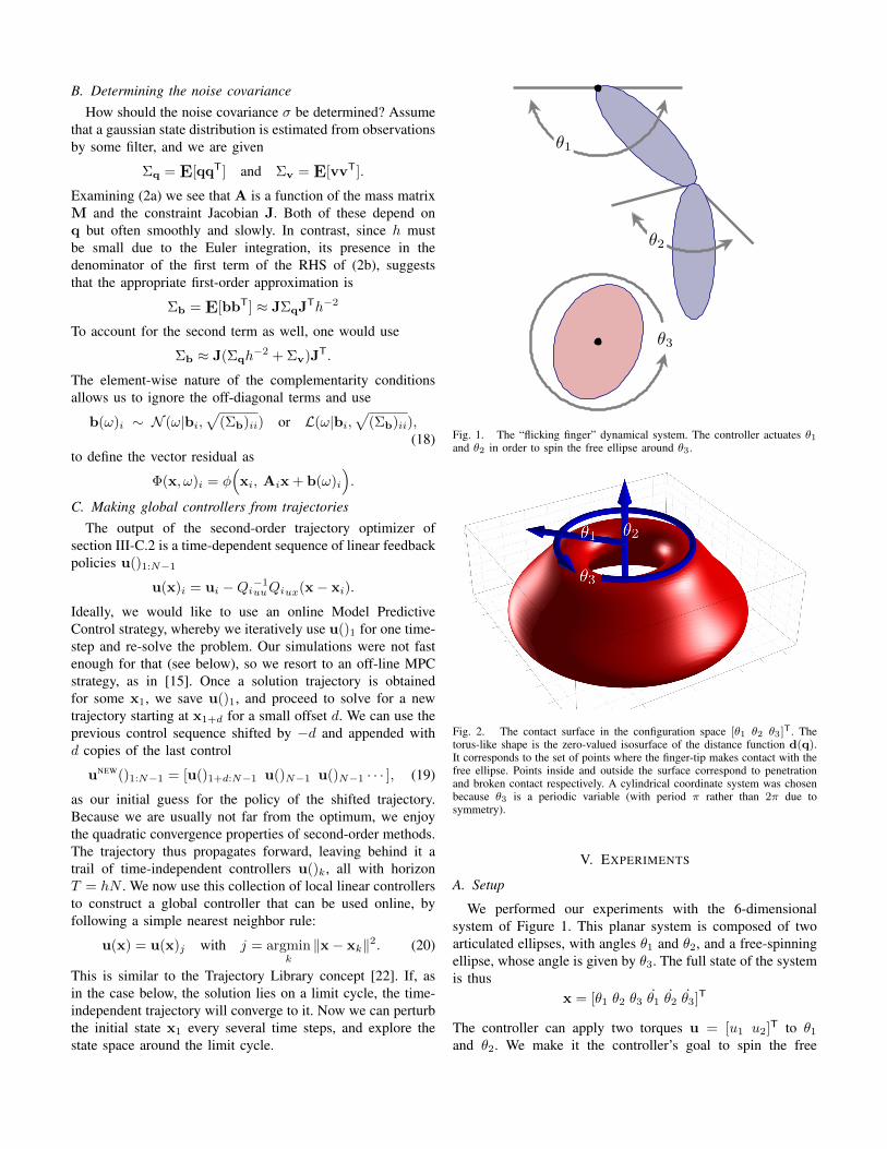
θ1

θ2

θ3

Fig. 1. The “flicking finger” dynamical system. The controller actuates θ1and θ2 in order to spin the free ellipse around θ3.

Fig. 2. The contact surface in the configuration space [θ1 θ2 θ3]T. Thetorus-like shape is the zero-valued isosurface of the distance function d(q).It corresponds to the set of points where the finger-tip makes contact with thefree ellipse. Points inside and outside the surface correspond to penetrationand broken contact respectively. A cylindrical coordinate system was chosenbecause θ3 is a periodic variable (with period π rather than 2π due tosymmetry).

V. EXPERIMENTS

A. Setup

We performed our experiments with the 6-dimensionalsystem of Figure 1. This planar system is composed of twoarticulated ellipses, with angles θ1 and θ2, and a free-spinningellipse, whose angle is given by θ3. The full state of the systemis thus

x = [θ1 θ2 θ3 θ1 θ2 θ3]T

The controller can apply two torques u = [u1 u2]T to θ1and θ2. We make it the controller’s goal to spin the free

ellipse in the positive direction, by defining a negative state-cost proportional to θ3 with a quadratic control-cost:

`(x,u) = −cxθ3 + cu‖u‖2

Note that it would be very difficult to solve this task withcontrol techniques that force the system to a pre-plannedtrajectory, since it is not clear how such a trajectory wouldbe found.

In Figure 2, we depict the d(q) = 0 isosurface in theconfiguration space [θ1 θ2 θ3]T.

B. Parameters and methodsThe following values can all be assumed to have the

appropriate units of a self consistent unit system (e.g. MKS).The major and minor radii of the finger ellipses are .8 and.25 respectively. Those of the free ellipse are .7 and .5. Themasses and moments of inertia correspond to a mass densityof 1. The vertical distance between the two anchors (blackdots in Figure 1) is 3. Angle limits are −π ≤ θ1 ≤ 0 and−2π/3 ≤ θ2 ≤ 0. The drag coefficients of the finger joints andof the free ellipse axis are .2, .2 and .7, respectively. Gravityin the vertical direction is -4. The control-cost coefficientswere cu = 0.05 and cx = 1. The time step h = 0.05 andthe number of time steps per trajectory N = 75, for a timehorizon of T = 3.5.

Both angle constraints and the contact constraint weresatisfied with impulses, as described in section III-A. We useda friction coefficient of µ = 0.5, with the friction modelof [9]. Since we did not estimate the dynamics, we used aconstant

√(Σb)ii = 0.1, which was chosen as a trade-off

between good convergence and small softening of the contact(described below). For the SLCP residual, both (15) and (17)gave qualitatively similar results, and we used (17) in theresults below, because it is computationally cheaper.

We avoided the matrix inversions of (2) by directly solvingthe (stochastic) mixed complementarity problem of (1). Thisis easy to do with NCP functions, by setting φ(a, b) = b forthose indexes where equality is desired.

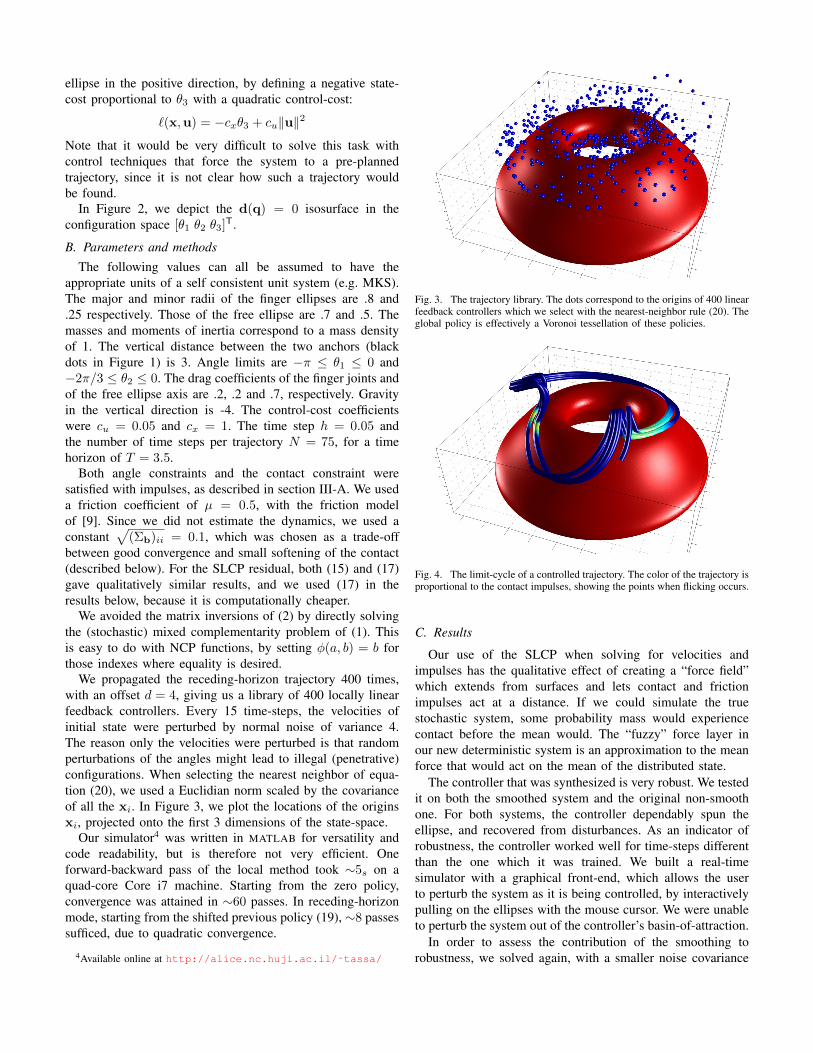
We propagated the receding-horizon trajectory 400 times,with an offset d = 4, giving us a library of 400 locally linearfeedback controllers. Every 15 time-steps, the velocities ofinitial state were perturbed by normal noise of variance 4.The reason only the velocities were perturbed is that randomperturbations of the angles might lead to illegal (penetrative)configurations. When selecting the nearest neighbor of equa-tion (20), we used a Euclidian norm scaled by the covarianceof all the xi. In Figure 3, we plot the locations of the originsxi, projected onto the first 3 dimensions of the state-space.

Our simulator4 was written in MATLAB for versatility andcode readability, but is therefore not very efficient. Oneforward-backward pass of the local method took ∼5s on aquad-core Core i7 machine. Starting from the zero policy,convergence was attained in ∼60 passes. In receding-horizonmode, starting from the shifted previous policy (19), ∼8 passessufficed, due to quadratic convergence.

4Available online at http://alice.nc.huji.ac.il/˜tassa/

Fig. 3. The trajectory library. The dots correspond to the origins of 400 linearfeedback controllers which we select with the nearest-neighbor rule (20). Theglobal policy is effectively a Voronoi tessellation of these policies.

Fig. 4. The limit-cycle of a controlled trajectory. The color of the trajectory isproportional to the contact impulses, showing the points when flicking occurs.

C. Results

Our use of the SLCP when solving for velocities andimpulses has the qualitative effect of creating a “force field”which extends from surfaces and lets contact and frictionimpulses act at a distance. If we could simulate the truestochastic system, some probability mass would experiencecontact before the mean would. The “fuzzy” force layer inour new deterministic system is an approximation to the meanforce that would act on the mean of the distributed state.

The controller that was synthesized is very robust. We testedit on both the smoothed system and the original non-smoothone. For both systems, the controller dependably spun theellipse, and recovered from disturbances. As an indicator ofrobustness, the controller worked well for time-steps differentthan the one which it was trained. We built a real-timesimulator with a graphical front-end, which allows the userto perturb the system as it is being controlled, by interactivelypulling on the ellipses with the mouse cursor. We were unableto perturb the system out of the controller’s basin-of-attraction.

In order to assess the contribution of the smoothing torobustness, we solved again, with a smaller noise covariance

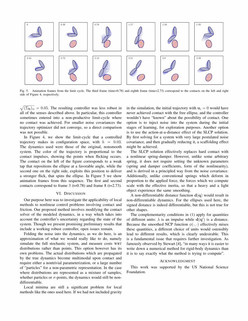
0 0.39 0.78 1.17 1.56 1.95

2.34 2.73 3.12 3.51 3.9 4.29

Fig. 5. Animation frames from the limit cycle. The third frame (time=0.78) and eighth frame (time=2.73) correspond to the contacts on the left and rightside of Figure 4, respectively.

√(Σb)ii = 0.05. The resulting controller was less robust in

all of the senses described above. In particular, this controllersometimes entered into a non-productive limit-cycle whereno contact was achieved. For smaller noise covariances thetrajectory optimizer did not converge, so a direct comparisonwas not possible.

In Figure 4, we show the limit-cycle that a controlledtrajectory makes in configuration space, with h = 0.03.The dynamics used were those of the original, nonsmoothsystem. The color of the trajectory is proportional to thecontact impulses, showing the points when flicking occurs.The contact on the left of the figure corresponds to a weaktap that repositions the ellipse at a favorable angle, while thesecond one on the right side, exploits this position to delivera stronger flick, that spins the ellipse. In Figure 5 we showanimation frames from this sequence. The first and secondcontacts correspond to frame 3 (t=0.78) and frame 8 (t=2.73).

VI. DISCUSSION

Our purpose here was to investigate the applicability of localmethods to nonlinear control problems involving contact andfriction. Our proposed method involves modifying the contactsolver of the modeled dynamics, in a way which takes intoaccount the controller’s uncertainty regarding the state of thesystem. Though we present promising preliminary results thatinclude a working robust controller, open issues remain.

Folding the noise into the dynamics, as we do here, is anapproximation of what we would really like to do, namelysimulate the full stochastic system, and measure costs WRTdistributions rather than points. This option however has itsown problems. The actual distributions which are propagatedby the true dynamics become multimodal upon contact andrequire either a nontrivial parameterization, or a large numberof “particles” for a non-parametric representation. In the casewhere distributions are represented as a mixture of samples,whether particles or σ-points, the dynamics would still be non-differentiable.

Local minima are still a significant problem for localmethods like the ones used here. If we had not included gravity

in the simulation, the initial trajectory with ui = 0 would havenever achieved contact with the free ellipse, and the controllerwouldn’t have “known” about the possibility of contact. Oneoption is to inject noise into the system during the initialstages of learning, for exploration purposes. Another optionis to use the action-at-a-distance effect of the SLCP solution.By first solving for a system with very large postulated noisecovariance, and then gradually reducing it, a scaffolding effectmight be achieved.

The SLCP solution effectively replaces hard contact witha nonlinear spring-damper. However, unlike some arbitraryspring, it does not require setting the unknown parameters(spring and damper coefficients, form of the nonlinearity),and is derived in a principled way from the noise covariance.Additionally, unlike conventional springs which deform inproportion to the applied force, the forces which we computescale with the effective inertia, so that a heavy and a lightobject experience the same smoothing.

A non-differentiable distance function d(q) would result innon-differentiable dynamics. For the ellipses used here, thesigned distance is indeed differentiable, but this is not true forother shapes.

The complementarity conditions in (1) apply for quantitiesof different units: λ is an impulse while d(q′) is a distance.Because the smoothed NCP function φ(·, ·) effectively mixesthese quantities, a different choice of units would ostensiblylead to different results, which is clearly undesirable. Thisis a fundamental issue that requires further investigation. Asfamously observed by Stewart [4], “in many ways it is easier towrite down a numerical method for rigid-body dynamics thanit is to say exactly what the method is trying to compute”.

ACKNOWLEDGMENT

This work was supported by the US National ScienceFoundation.

REFERENCES

[1] X. Chen and M. Fukushima, “Expected residual minimization methodfor stochastic linear complementarity problems,” Math. Oper. Res.,vol. 30, no. 4, pp. 1022–1038, 2005.

[2] F. Pfeiffer and C. Glocker, Multibody dynamics with unilateral contacts.Wiley-VCH, 1996.

[3] E. Westervelt, Feedback control of dynamic bipedal robot locomotion.Boca Raton: CRC Press, 2007.

[4] D. E. Stewart, “Rigid-Body dynamics with friction and impact,” SIAMReview, vol. 42, no. 1, pp. 3–39, 2000.

[5] J. J. Moreau, “Unilateral contact and dry friction in finite freedomdynamics,” Nonsmooth mechanics and Applications, p. 1–82, 1988.

[6] F. A. Potra, M. Anitescu, B. Gavrea, and J. Trinkle, “A linearlyimplicit trapezoidal method for integrating stiff multibody dynamicswith contact, joints, and friction,” International Journal for NumericalMethods in Engineering, vol. 66, no. 7, pp. 1079–1124, 2006.

[7] E. Todorov, “Implicit nonlinear complementarity: a new approach tocontact dynamics,” in International Conference on Robotics and Au-tomation, 2010.

[8] M. Anitescu and F. A. Potra, “Formulating dynamic Multi-Rigid-Body contact problems with friction as solvable linear complementarityproblems,” Nonlinear Dynamics, vol. 14, no. 3, pp. 231–247, Nov. 1997.

[9] M. Anitescu, “Optimization-based simulation of nonsmooth rigid multi-body dynamics,” Mathematical Programming, vol. 105, no. 1, pp. 113–143, 2006.

[10] R. W. Cottle, J. Pang, and R. E. Stone, The Linear ComplementarityProblem. SIAM, Oct. 2009.

[11] S. C. Billups and K. G. Murty, “Complementarity problems,” Journalof Computational and Applied Mathematics, vol. 124, no. 1-2, pp. 303–318, Dec. 2000.

[12] C. Chen and O. L. Mangasarian, “A class of smoothing functionsfor nonlinear and mixed complementarity problems,” ComputationalOptimization and Applications, vol. 5, no. 2, pp. 97–138, Mar. 1996.

[13] L. S. Pontryagin, V. G. Boltyanskii, R. V. Gamkrelidze, and E. F.Mishchenko, The mathematical theory of optimal processes. Inter-science New York, 1962.

[14] P. Abbeel, A. Coates, M. Quigley, and A. Y. Ng, “An application ofreinforcement learning to aerobatic helicopter flight,” in Advances inNeural Information Processing Systems 19: Proceedings of the 2006Conference, 2007, p. 1.

[15] Y. Tassa, T. Erez, and W. Smart, “Receding horizon differential dynamicprogramming,” in Advances in Neural Information Processing Systems20, J. Platt, D. Koller, Y. Singer, and S. Roweis, Eds. Cambridge, MA:MIT Press, 2008, p. 1465–1472.

[16] R. Tedrake, “LQR-Trees: feedback motion planning on sparse random-ized trees,” in Proceedings of Robotics: Science and Systems (RSS),2009.

[17] M. Toussaint, “Robot trajectory optimization using approximate infer-ence,” in Proceedings of the 26th Annual International Conference onMachine Learning, 2009.

[18] D. E. Stewart and M. Anitescu, “Optimal control of systems withdiscontinuous differential equations,” Numerische Mathematik, 2009.

[19] W. H. Fleming and H. M. Soner, Controlled Markov processes andviscosity solutions. Springer Verlag, 2006.

[20] M. Fukushima and G. lin, “Stochastic equilibrium problems and stochas-tic mathematical programs with equilibrium constraints: A survey,”Pacific Journal of Optimization, vol. to appear, 2010.

[21] X. Chen and P. Tseng, “Non-Interior continuation methods for solvingsemidefinite complementarity problems,” Mathematical Programming,vol. 95, no. 3, pp. 431–474, Mar. 2003.

[22] M. Stolle and C. G. Atkeson, “Policies based on trajectory libraries,” inProceedings of the International Conference on Robotics and Automa-tion (ICRA 2006), 2006.