Stochastic Coverage in Heterogeneous Sensor Networks

Stochastic Coverage in Heterogeneous SensorNetworks∗

LOUKAS LAZOS and RADHA POOVENDRAN

University of Washington

We study the problem of coverage in planar heterogeneous sensor networks. Coverage is a perfor-mance metric that quantifies how well a field of interest is monitored by the sensor deployment.To derive analytical expressions of coverage for heterogeneous sensor networks, we formulate thecoverage problem as a set intersection problem, a problem studied in Integral Geometry. Com-pared to previous analytical results, our formulation allows us to consider a network model where,sensors are deployed according to an arbitrary stochastic distribution; sensing areas of sensorsneed not follow the unit disk model but can have any arbitrary shape; sensors need not have anidentical sensing capability. Furthermore, our formulation does not assume deployment of sensorsover an infinite plane and, hence, our derivations do not suffer from the border effect problemarising in a bounded field of interest. We compare our theoretical results with the spatial Pois-son approximation that is widely used in modeling coverage. By computing the Kullback-Leiblerand Total Variation distance between the probability density functions derived via our theoreti-cal results, the Poisson approximation, and the simulation, we show that our formulas provide amore accurate representation of the coverage in sensor networks. Finally, we provide examples ofcalculating network parameters such as the network size and sensing range in order to achieve adesired degree of coverage.

Categories and Subject Descriptors: C.2 [Computer System Organization]: Computer - Com-munication Networks; C.2.1 [Network Architecture and Design]: Distributed networks—Network topology

General Terms: Algorithm, Design, Performance

Additional Key Words and Phrases: Stochastic, Coverage, Sensor networks, Heterogeneous

1. INTRODUCTION

Sensor networks are becoming an attractive solution for many commercial and mil-itary applications due to their low cost, ease of deployment, unattended operation,and wealth of useful information that they can collect. Typical applications in-clude emergency rescue, ambient control, environmental monitoring, home healthcare and surveillance networks [Akyildiz et al. 2002; Mainwaring et al. 2002].

One of the primary tasks of sensor networks is to monitor a Field of Interest(FoI). Sensors may monitor physical properties such as temperature, humidity, airquality, or track the motion of objects moving within the FoI. In many cases sensornetworks may initiate an automated reaction to the observed events (actuation

∗A preliminary version of this article appears in WiOpt 2006.Permission to make digital/hard copy of all or part of this material without fee for personalor classroom use provided that the copies are not made or distributed for profit or commercialadvantage, the ACM copyright/server notice, the title of the publication, and its date appear, andnotice is given that copying is by permission of the ACM, Inc. To copy otherwise, to republish,to post on servers, or to redistribute to lists requires prior specific permission and/or a fee.c© 20YY ACM 0000-0000/20YY/0000-0001 $5.00

ACM Journal Name, Vol. V, No. N, Month 20YY, Pages 1–0??.

2 · Loukas Lazos and Radha Poovendran

networks). As an example, motion detection sensors may trigger the lights toturn on after motion has been detected, or sensors monitoring a patient’s bloodstream may automatically increase the intake of sugars in the event of low sugarlevel detection. In actuation networks, in order to guarantee the robustness of thedecision mechanism, it is critical to improve the accuracy and reduce the probabilityof false alarm.

While robustness may be achieved by pursuing a multimodal approach that in-volves multiple consistency checks before any actuation decision is made, robustnessdepends, to a high degree, on the availability of monitoring information. In order toevaluate a specific event, one needs to have sufficient observations of the event. Onthe other hand, the number of available observations is directly related to the num-ber of sensors able to sense a particular event. Hence, to improve the robustness ofthe system, one needs to increase the availability of the collected information.

The availability of monitoring information can be measured by computing thecoverage of the FoI, achieved by the sensor network deployment. Coverage quan-tifies how well a FoI is monitored1. The coverage problem has been studied underdifferent objectives, depending on the requirements and constraints of the appli-cations. If the location of the deployed sensors can be pre-selected, the coverageproblem reduces to the problem of finding the optimal placement for sensors suchthat a target coverage is met [Kar and Banerjee 2003; Poduri and Sukhatme 2004].

However, for large sensor networks, it is impractical to perform deterministiccoverage of the FoI, since the number of sensors that need to be placed is oftenprohibitively large. Instead, sensors are deployed in the field of interest accordingto a pre-selected distribution. For stochastically deployed sensor networks, thecoverage problem quantifies how well the FoI is monitored when a number ofsensors is deployed according to a known distribution. This problem is also knownas the stochastic coverage problem [Koushanfar et al. 2001; Meguerdichian et al.2001; Liu and Towsley 2004; Miorandi and Altman 2005; Xing et al. 2005]. In thisarticle, we analyze the following stochastic coverage problem. Given a planar FoIand N sensors deployed according to a known distribution, compute the fractionof the FoI that is covered by at least k sensors (k ≥ 1). The problem can also berephrased as, given a FoI and a sensor distribution, how many sensors must bedeployed in order for every point in the field of interest to be covered by at least ksensors with a probability p (k-coverage problem) [Xing et al. 2005].

1.1 Our Contributions

In this article, we make the following contributions. We formulate the problem ofcoverage in sensor networks as a set intersection problem. We use results from Inte-gral Geometry to derive analytical expressions quantifying the coverage achieved bystochastic deployment of sensors into a planar field of interest. Compared to previ-ous analytical results [Liu and Towsley 2004; Poduri and Sukhatme 2004, Miorandiand Altman 2005], our formulation allows us to consider a heterogeneous sensingmodel, where sensors need not have an identical sensing capability. In addition, our

1Once the information has been collected by the sensors, an additional mechanism known asdata aggregation [Krishnamachari et al. 2002], is required to timely communicate the availableinformation for processing. We do not address the aggregation problem in this article.

ACM Journal Name, Vol. V, No. N, Month 20YY.

Stochastic Coverage in Heterogeneous Sensor Networks · 3

approach is applicable to scenarios where the sensing area of a sensor does not fol-low the unit disk model, but has any arbitrary shape. To the best of our knowledge,only [Miorandi and Altman 2005] considers a heterogeneous sensing model, thoughobtaining results that eventually only incorporate the mean value of the sensingrange in the coverage computation. Furthermore, the formulation in [Miorandi andAltman 2005] considers only uniformly deployed sensors. In our approach, sensorscan be deployed according to any distribution.

We provide formulas for k-coverage in the case of heterogeneous sensing areas,as well as the simplified forms in the case of identical sensing areas. We verifyour theoretical results by performing extensive simulations that show an almostexact match between our theoretical derivation and simulation. We compare ouranalytical formulas with previous analytic results [Liu and Towsley 2004; Poduriand Sukhatme 2004, Miorandi and Altman 2005] by computing the Kullback-Leiblerdistance [Cover and Thomas 1991] and illustrate that our expressions provide ahigher accuracy, since they do not suffer from the border effects [Bettstetter andKrause 2001; Bettstetter and Zangl 2002]. Finally, we provide examples on how touse our analytical expressions to compute the number of sensors that need to bedeployed, in order to cover a FoI with a desired probability.

The rest of the article is organized as follows. In Section 2, we present relatedwork. In Section 3, we state our network model and formulate the coverage problemas a set intersection problem. In Section 4, we derive analytical expressions forcoverage for both heterogeneous and homogeneous sensor networks. In Section 5,we validate our analytical expressions, by computing coverage via simulation, andprovide examples of computing the coverage in randomly deployed sensor networks.Section 6 presents our conclusions.

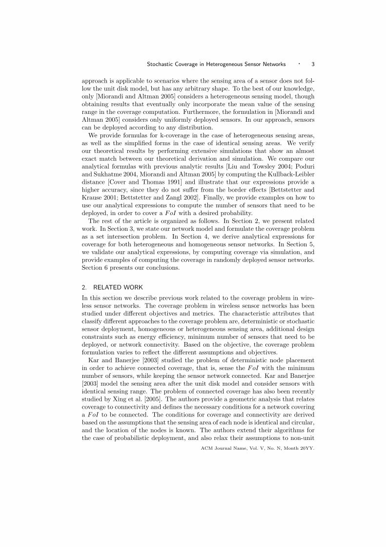
2. RELATED WORK

In this section we describe previous work related to the coverage problem in wire-less sensor networks. The coverage problem in wireless sensor networks has beenstudied under different objectives and metrics. The characteristic attributes thatclassify different approaches to the coverage problem are, deterministic or stochasticsensor deployment, homogeneous or heterogeneous sensing area, additional designconstraints such as energy efficiency, minimum number of sensors that need to bedeployed, or network connectivity. Based on the objective, the coverage problemformulation varies to reflect the different assumptions and objectives.

Kar and Banerjee [2003] studied the problem of deterministic node placementin order to achieve connected coverage, that is, sense the FoI with the minimumnumber of sensors, while keeping the sensor network connected. Kar and Banerjee[2003] model the sensing area after the unit disk model and consider sensors withidentical sensing range. The problem of connected coverage has also been recentlystudied by Xing et al. [2005]. The authors provide a geometric analysis that relatescoverage to connectivity and defines the necessary conditions for a network coveringa FoI to be connected. The conditions for coverage and connectivity are derivedbased on the assumptions that the sensing area of each node is identical and circular,and the location of the nodes is known. The authors extend their algorithms forthe case of probabilistic deployment, and also relax their assumptions to non-unit



Reference Sensor Deployment Sensing Model

[Kar and Banerjee 2003] Deterministic Unit Disk

[Xing et al. 2005] Known Location Unit Disk

[Poduri and Sukhatme 2004] Deterministic Unit Disk

[Meguerdichian et al. 2001] Known Location Any

[Koushanfar et al. 2001] Known Location Any

[Liu and Towsley 2004] Random Any

[Li et al. 2003] Known Location Any

[Miorandi and Altman 2005] Random Any

Our work Stochastic Any

Reference Heterogeneous Model Additional Constraints

[Kar and Banerjee 2003] No Connectivity

[Xing et al. 2005] No Connectivity

[Poduri and Sukhatme 2004] No K-connectivity

[Meguerdichian et al. 2001] Yes Worst Coverage

[Koushanfar et al. 2001] Yes Best, Worst Coverage

[Liu and Towsley 2004] No None

[Li et al. 2003] Yes Best, Worst Coverage

[Miorandi and Altman 2005] Yes None

Our work Yes None

Table I. Comparison of the related work on the coverage problem for sensor networks, in terms ofassumptions and constraints. Sensor deployment refers to the deployment method, deterministicor stochastic as well as the prior knowledge about the location of the sensors. Sensing model refersto the assumptions about the sensing areas. Heterogeneous model refers to whether the analysissupports sensors with heterogeneous sensing capabilities. Additional constraints refers to otherobjectives set, such as connectivity, energy efficiency or minimization of the number of sensorsdeployed.

disk sensing areas, by approximating the real sensing area with the biggest possiblecircular area included in the real sensing area.

Poduri and Sukhatme [2004] study the problem of deterministic coverage underthe additional constraint that each sensor must have at least k neighbors. Theypropose a deployment strategy that would maximize the coverage while the degreeof each node is guaranteed to be at least k, under the assumption that the sensingrange of the sensors is isotropic.

Meguerdichian et al. [2001] study the problem of coverage, as a path exposureproblem. Using a generic sensing model and an arbitrary sensor distribution, theypropose a systematic method for discovering the minimum exposure path, that isthe path along which the network exhibits the minimum integral observability2.Koushanfar et al. [2001] investigate the problem of best- and worst-case coverage.In their formulation of the coverage problem, given the location of the sensors anda generic sensing model where the sensing ability of each sensor diminishes withdistance, the authors use Voronoi diagrams and Delaunay triangulation to computethe path that maximizes the smallest observability (best coverage) and the paththat minimizes the observability by all sensors (worst coverage). [Li et al. 2003]provide a decentralized and localized algorithm for calculating the best coverage.

2The integral observability is defined as the aggregate of the time that a target was observable bysensors while traversing a sensor network.



Liu and Towsley [2004] study the problem of stochastic coverage in large scalesensor networks. For a randomly distributed sensor network, the authors providethe fraction of the FoI covered by k sensors, the fraction of nodes that can beremoved without reducing the covered area as well as the ability of the networkto detect moving objects. The results presented by Liu and Towsley [2004] holdonly for randomly (uniformly) deployed networks and under the assumption thatthe sensing area of each sensor is identical. Furthermore, the analysis presentedby Liu and Towsley [2004] suffers from the border effects problem, illustrated in[Bettstetter and Krause 2001; Bettstetter and Zangl 2002]. The results hold as-ymptotically under the assumption that the FoI expands infinitely in the plane,while the density of the sensor deployment remains constant.

Miorandi and Altman [2005] study the stochastic coverage problem in ad hocnetworks in the presence of channel randomness. For a randomly deployed sensornetwork, the authors analyze the effects of shadowing and fading to the connectivityand coverage. They show that the in the case of channel randomness, the coverageproblem can still be modeled with the assistance of the spatial Poisson distribution,by using expected size of the sensing area of sensors. While the results by Miorandiand Altman [2005] are applicable to heterogeneous sensor networks they hold onlyfor randomly deployed networks, and are impacted from the border effects problem[Bettstetter and Krause 2001; Bettstetter and Zangl 2002], as noted by Miorandiand Altman [2005].

Gupta et al. [2003] study the problem of selecting the minimum number of sensorsfrom a set of sensors that are randomly (uniformly) deployed such that the FoI iscovered, and the selected sensors form a connected network. The authors providecentralized and decentralized heuristic algorithms that perform within a boundfrom the optimal solution. The authors assume that the sensing area of the sensorscan have any convex shape, and sensors can have heterogeneous capabilities. As arequirement, the position as well as the shape and size of each sensing area mustbe known after deployment.

Compared to previous work that derives analytical coverage expressions [Liu andTowsley 2004; Poduri and Sukhatme 2004; Miorandi and Altman 2005], our for-mulation allows us to consider a network model where, (a) sensors can be deployedaccording to any distribution, (b) sensors can have a sensing area of any arbitraryshape, (c) sensors can have heterogeneous sensing areas. Furthermore, our formu-lation does not suffer from the border effects problem. Table 2 summarizes thedifferent assumptions and objectives of previous works.

3. NETWORK MODEL, PROBLEM FORMULATION & BACKGROUND

3.1 Network model

In many wireless sensor network applications, it is not practical to deploy thesensors deterministically due to the large number of sensors that need to be deployedand/or the type of environment where they are deployed. As an example, sensorsmay be dropped off an aircraft into a forest in order to monitor environmentalparameters such as humidity, temperature, air quality etc. Furthermore, in manyapplications, sensors do not remain static, even after they have been placed inthe FoI. Environmental changes, such as air, rain, river streams etc., may move



−50

5

−5

0

5

0.005

0.01

0.015

0.02

0.025

0.03

−6 −4 −2 0 2 4 6

−4

−3

−2

−1

0

1

2

3

4

(a) (b)

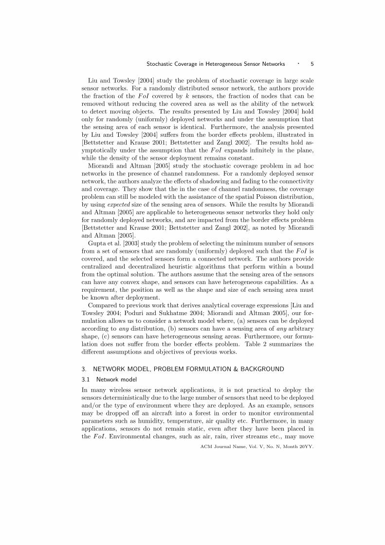
Fig. 1. (a) A two-dimensional Gaussian distribution with mean value E(X,Y ) =[0, 0], (b) projection of the Gaussian distribution into the planar field.

sensors over time [Szewczyk et al. 2004]. For these types of applications the relevantcoverage question that quantifies the availability of monitoring information is howmany sensors do we need to deploy in order to achieve the desired coverage with aprobability higher than a threshold value.

Furthermore, sensors may not be deployed according to a random distributionover the FoI. As an example, a subset of points in the FoI may be of greater interestthan other points and, hence, must be monitored by a larger number of sensors. Insuch a case, more sensors may be deployed around the critical subset of points. Forexample, a desired heterogeneous coverage may be achieved by deploying sensorsaccording to a two-dimensional Gaussian distribution. In figure 1(a), we showthe probability density function for a two-dimensional Gaussian distribution withmean value equal to E(X, Y ) = [0, 0]. In figure 1(b), we show the projection of theGaussian probability density function into the planar field.

Since the sensor deployment distribution may vary, it is desirable to have ana-lytical coverage results that can incorporate any arbitrary sensor distribution. Inour analysis, we study the stochastic coverage problem when sensors are deployedaccording to any distribution and derive analytical results even in the case of non-uniform sensor distribution.

In addition, it is desirable to develop analytical coverage formulas that hold notonly for homogeneous, but also for heterogeneous sensor networks. Heterogeneityin the sensing area of sensors may be due to the following reasons. First, themanufacturing process for sensors does not guarantee that sensors are equippedwith identical hardware, able to produce an identical sensing model. Furthermore,the heterogeneity of the environment where the sensors are deployed distorts thesensing capabilities of the sensors measured in an ideal environment. Finally, thesensor network may consist of sensors with different sensing capabilities by design(hierarchical sensor networks). We analyse the coverage problem adopting a generalsensing model that captures the heterogeneity in the sensing capabilities of sensors.

In this article we adopt the following network model.ACM Journal Name, Vol. V, No. N, Month 20YY.


Field of Interest A0 Sensing area AiSensing area Ai

si

Fi

Li

(a) (b)

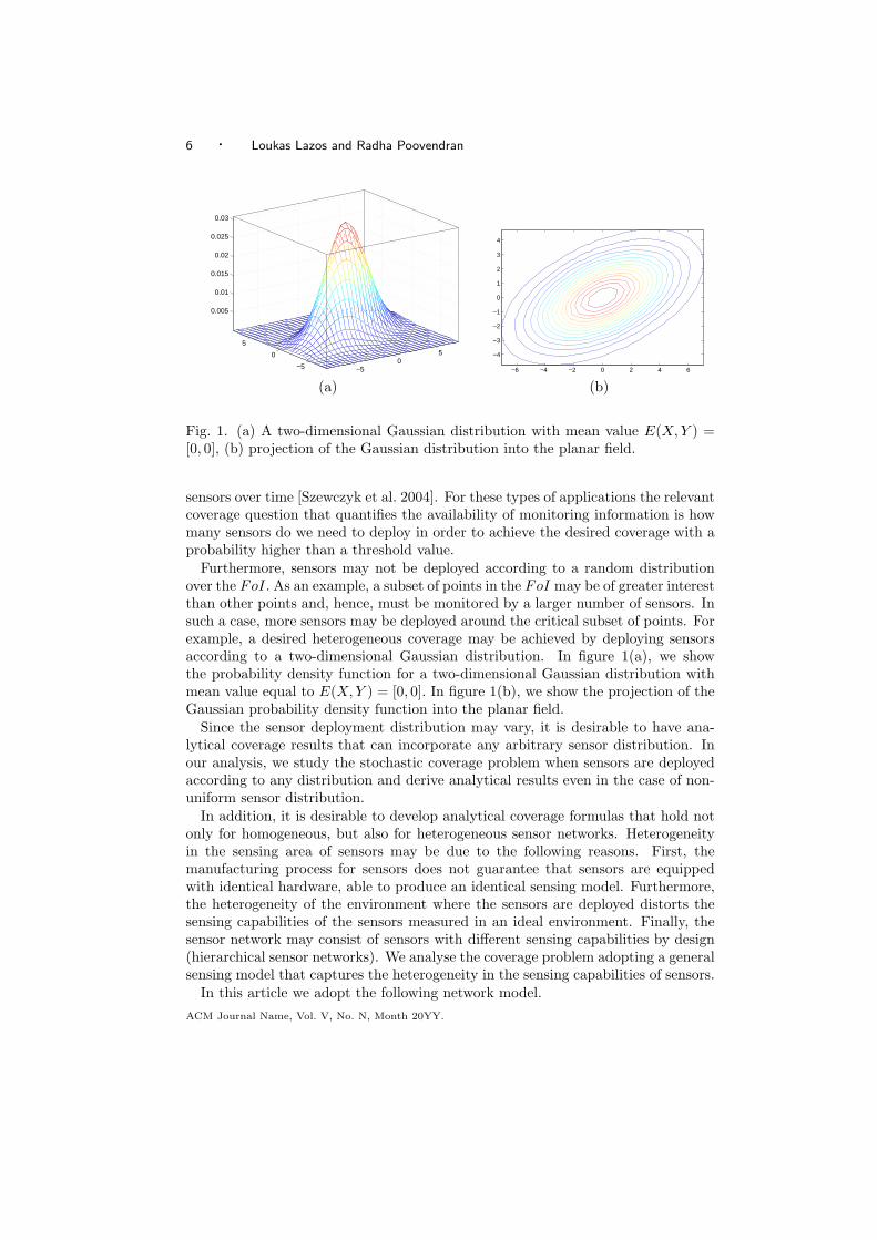
Fig. 2. (a) A heterogeneous sensor network with randomly deployed sensors coveringan FoI A0, (b) The sensing area Ai of a sensor si.

- Field of Interest (FoI): Let A0 denote the Field of Interest (FoI) we want tomonitor, with area F0 and perimeter L0. We assume that the FoI is planar andcan have any arbitrary shape.

- Sensing area: Let Ai denote the sensing area of each sensor si, i = 1 . . . N,with Fi, Li denoting the size of the area and perimeter of Ai. The sensing areacan have any arbitrary shape.

- Sensor deployment: We assume that N sensors are deployed according to adistribution Y (A0) and in such a way that they sense some part of the FoI. Forsensing, it is not necessary that the sensors are located within the FoI. Instead,we require that sensors can monitor some part of the FoI even if they are locatedoutside of it.

3.2 Problem Formulation

We study the following stochastic coverage problem.

Stochastic coverage problem: Given a FoI A0 of area F0 and perimeter L0,sensed by N sensors with each sensor si having a sensing area Ai of size Fi andperimeter Li deployed in the plane according to a distribution Y (A0), compute thefraction of A0 that is sensed by at least k sensors, i.e. the fraction that is k-covered.

This problem is equivalent to computing the probability that a randomly selectedpoint P ∈ A0 is sensed by at least k sensors. The stochastic coverage problem canbe mapped to the following set intersection problem.

Set intersection problem: Let S0 be a fixed bounded set defined as a collection ofpoints in the plane, and let F0 and L0 denote the area and perimeter of S0. Let Nbounded sets Si (i = 1 . . . N) of size Fi and perimeter Li be dropped in the plane ofS0 according to a distribution Y (S0) and in such a way that every set Si intersectswith S0. Compute the fraction of S0 where at least k out of the N sets Si intersect.



In the mapping of the stochastic coverage problem to the set intersection problem,the fixed bounded set S0 corresponds to the FoI A0. The N bounded sets droppedaccording to the distribution Y (S0) correspond to the sensing areas of the N sensorsdeployed according to the distribution Y (A0). By computing the fraction of the setS0, where at least k out of N sets Si intersect, we equivalently compute the fractionof the FoI that is k-covered3. In figure 2(a), we show a sensor network randomlydeployed over a FoI. In figure 2(b), we show the sensing area of a sensor si. Notethat our formulation does not require the FoI to be infinitely extending in the plane.Instead, the FoI has to be a bounded region and, hence, our formulation does notsuffer from the border effects problem [Bettstetter and Krause 2001; Bettstetterand Zangl 2002].

The set intersection problem has been a topic of research of Integral Geometryand Geometric Probability [Santalo 1936; Santalo 1976; Miles 1969; Stoka 1969;Filipescu 1971]. In the following section, we show that the results obtained for theset intersection problem can be used to analyse the coverage problem in wirelesssensor networks. Before we provide analytical coverage expressions based on ourformulation, we present relevant background.

3.3 Background on Integral Geometry

In this section, we present relevant background on Integral Geometry that we usein Section 4 for deriving analytical coverage expressions based on our formulation.Interested reader is referred to [Santalo 1936; Santalo 1976; Miles 1969; Stoka 1969;Filipescu 1971], as reference to Integral Geometry. We first introduce the notion ofmotion for a point P in the plane, defined as follows [Santalo 1976]:

Definition 3.1. Motion in the Plane: Let P (xi, yi) denote a point in theEuclidean plane, where xi, yi denote Cartesian coordinates. A motion is defined asa transformation T : P (xi, yi) → P ′(x′i, y

′i) such that,

x′i = xi cos φ− yi sin φ + x, y′i = xi sin φ + yi cosφ + y

−∞ < x < ∞, −∞ < y < ∞, 0 ≤ φ ≤ 2π. (1)

Any motion of a point P or a set of points4 A, is characterized by the horizontaldisplacement α, the vertical displacement β and the rotation φ. A group of motionsM denotes a collection (set) of transformations in the Euclidean plane, i.e. therespective range for the 3-space (α, β, φ).

To quantify a group of motions M in the plane, we must define an appropriatemeasure for the set of transformations of A determined by M. Such a measure iscalled the kinematic measure and it must be invariant to the initial position of A,invariant under translation as well as invariant under inversion of the motion. Theneed for such invariance will become clear in the example following the definitionof the kinematic measure.

To define the kinematic measure we must introduce the notion of kinematic den-sity for the group of motions M of a point P (x, y) or set of points A in the plane.

3Due to their equivalence, A0 and S0 as well as the terms sensing area and set are used inter-changeably in the rest of the article.4In the case of a set of points, the set can be represented by a single point O based on which allother points are determined.



(a) (b)

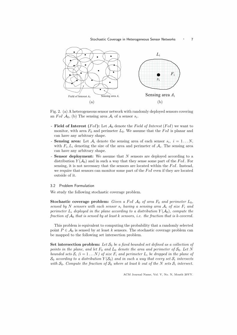
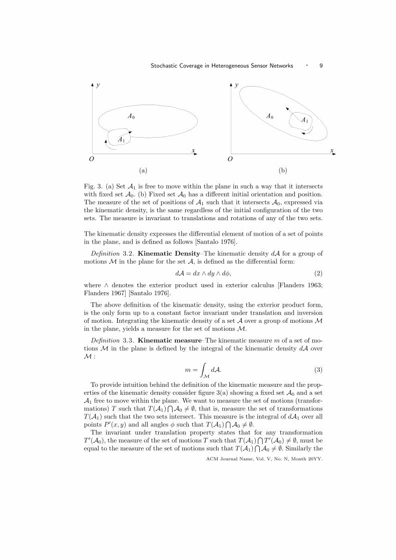
Fig. 3. (a) Set A1 is free to move within the plane in such a way that it intersectswith fixed set A0. (b) Fixed set A0 has a different initial orientation and position.The measure of the set of positions of A1 such that it intersects A0, expressed viathe kinematic density, is the same regardless of the initial configuration of the twosets. The measure is invariant to translations and rotations of any of the two sets.

The kinematic density expresses the differential element of motion of a set of pointsin the plane, and is defined as follows [Santalo 1976].

Definition 3.2. Kinematic Density–The kinematic density dA for a group ofmotions M in the plane for the set A, is defined as the differential form:

dA = dx ∧ dy ∧ dφ, (2)

where ∧ denotes the exterior product used in exterior calculus [Flanders 1963;Flanders 1967] [Santalo 1976].

The above definition of the kinematic density, using the exterior product form,is the only form up to a constant factor invariant under translation and inversionof motion. Integrating the kinematic density of a set A over a group of motions Min the plane, yields a measure for the set of motions M.

Definition 3.3. Kinematic measure–The kinematic measure m of a set of mo-tions M in the plane is defined by the integral of the kinematic density dA overM :

m =∫

MdA. (3)

To provide intuition behind the definition of the kinematic measure and the prop-erties of the kinematic density consider figure 3(a) showing a fixed set A0 and a setA1 free to move within the plane. We want to measure the set of motions (transfor-mations) T such that T (A1)

⋂A0 6= ∅, that is, measure the set of transformationsT (A1) such that the two sets intersect. This measure is the integral of dA1 over allpoints P ′(x, y) and all angles φ such that T (A1)

⋂A0 6= ∅.The invariant under translation property states that for any transformation

T ′(A0), the measure of the set of motions T such that T (A1)⋂

T ′(A0) 6= ∅, must beequal to the measure of the set of motions such that T (A1)

⋂A0 6= ∅. Similarly theACM Journal Name, Vol. V, No. N, Month 20YY.


measure must be invariant to any translations of set A1. Furthermore, the measureis invariant to the order by which we consider the possible motions of the set A1,or the initial positioning of sets A0,A1[Santalo1976]. Figure 3(b) shows a differentpositioning and orientation of the fixed set A0 that could be due to the applicationof a translation or a different initial positioning.

The quotient of the measure of a group of motions Z over the measure of a groupof motions M in the plane, where Z ⊆ M yields the probability p(Z) for thatgroup of motions to occur:

p(Z) =m(Z)m(M)

. (4)

The kinematic measure allows us to compute the geometric probability for a spe-cific set configuration to occur, as depicted in (4). Equation (4), is used in ourformulation to derive the fraction of the FoI covered by a sensor deployment, as itis illustrated in the following section.

4. ANALYTICAL EVALUATION OF COVERAGE IN HETEROGENEOUS SENSORNETWORKS

In this section, we derive analytical expressions for stochastic coverage in heteroge-neous sensor networks. We first study the coverage problem for the case where onlyone sensor is deployed, by studying the intersection of two sets in a plane. We ini-tially consider a sensor with a sensing area of convex shape. When the sensing areais convex, only the size and perimeter of the sensing area are required to computecoverage. When the sensing area has a non-convex shape, additional informationsuch as the decomposition of the sensing area to a union of disjoint convex shapesis required. In Section 4.3 extend our results for non-convex sensing areas.

We modify our analytical formulas for the case where the sensor is deployedaccording to an arbitrary distribution. Using the results from the single sensordeployment, we generalize for the case where multiple sensors are deployed andcompute the fraction of the FoI covered by at least k sensors, when a total of Nsensors are deployed. Finally, we show how we can derive previous analytical results[Liu and Towsley 2004; Poduri and Sukhatme 2004] as specific cases of our model.

4.1 Random deployment of a single sensor

In this section, we analyze the simplest case where a sensor s1 is randomly deployedin the plane. We assume that s1 has a convex sensing area A1 of size F1 andperimeter L1. We want to compute the fraction of the FoI covered by the sensors1. The equivalent set intersection problem is as follows. Let A0,A1 denote twosets in a plane with A0 being fixed, while A1 can move freely within the plane.Assume that all positions of A1 are equiprobable (sensor si is deployed at random).Compute the fraction of A0 covered by A1.

Let A01 denote the intersection between sets A0,A1. Since A0,A1 are convex,A01 is also convex. The fraction fr(A0) of A0 covered by A1, is computed bynormalizing the size of the area of A01 over the size of A0. The intersection areabetween the two sets A0,A1 can be computed with tools from integral geometry[Santalo 1936; Santalo 1976;].ACM Journal Name, Vol. V, No. N, Month 20YY.


To compute fr(A0), we randomly select a point P ∈ A0. Let p(P ∈ A1) denotethe probability that P ∈ A1, that is, that point P belongs in the intersectionbetween the sets A0 and A1. Integrating p(P ∈ A1) over all P ∈ A0 yields theprobability that any point of A0 belongs to A1. Since all points are equiprobable,integration of p(P ∈ A1) over all P ∈ A0 also computes the area F01 of theintersection set between A0,A1. Normalizing F01 over the F0, yields the desiredfraction fr(A0). The following theorem holds for convex sets, and will be extendedin Section 4.3 for the case of non-convex sets [Santalo 1976].

Theorem 4.1. Let A0 be a fixed convex set of area F0 and perimeter L0, andlet A1 be a convex set of area F1 and perimeter L1, randomly dropped in the planein such a way that it intersects with A0. The probability that a randomly selectedpoint P ∈ A0 is covered by A1 is given by:

p(P ∈ A1) =2πF1

2π(F0 + F1) + L0L1. (5)

Proof. According to (4), in order to compute the probability that P is coveredby A1, we need to compute the quotient of the measure of all motions of A1 suchthat P ∈ A1, over the measure of the set of motions of A1 such that A0

⋂A1 6= ∅.The latter represents all possible positions where A1 can be dropped (recall thatas a constraint, we require that A1 always intersects A0). We now provide thecomputation of the two measures, also sketched in [Santalo 1936; Santalo 1976]:

m(A1 : P ∈ A0

⋂A1)

(i)=

∫

P∈A0TA1

dA1

(ii)=

∫

P∈A1

dA1

(iii)=

∫

P∈A1

dx ∧ dy

∫ 2π

0

dφ(iv)= 2πF1. (6)

In (i), we integrate the kinematic density dA1 of set A1 over all motions of A1 suchthat P ∈ A0

⋂A1. Since by assumption P ∈ A0 and A0 is fixed, we only need tointegrate over all P ∈ A1. In (ii), we integrate dA1 over all motions of A1 such thatP ∈ A1. In (iii), we express the kinematic density as its differential product form,and consider all possible rotations of A1 such that P ∈ A1. In (iv), the integral ofdx∧ dy over all P ∈ A1 is equal to the area F1 of A1. The integral of dφ over all φis equal to 2π since A1 can freely rotate around its reference point, leading to thevalue of 2πF1.

The result in (6) is intuitive. Given a fixed point P the number of translationmotions of the set A1 that can include P, is equal to the area F1 of A1. For eachposition of A1 that include P, we can rotate A1 a total of 2π positions before werepeat the initial configuration. Hence, the measure of positions of A1 such thatP ∈ A1 under both rotation and translation is equal to 2πF1.

Let P be a randomly selected point of the fixed set A0. All possible positions ofA1 that include P can be obtained by translating A1 according to the vector v, androtating A1 by φ ∈ [0, 2π]. The measure of all translation is F1 while the measureof all rotations is 2π, hence the measure of all positions such that P ∈ A1 is 2πF1.



We now compute the measure of all motions of A1 such that A0

⋂A1 6= 0 :

m(A1 : A0

⋂A1 6= ∅) (i)

=∫

A0TA1 6=∅

dA1

(ii)=

∫

A0TA1 6=∅

dx ∧ dy ∧ dφ

(iii)=

∫ 2π

0

(F0 + F1 + 2F01) dφ

(iv)= 2π(F0 + F1) + L0L1. (7)

In (i), we integrate the kinematic density dA1 of set A1 over all motions of A1

such that A0

⋂A1 6= ∅. In (ii), we write the kinematic density in its expandeddifferential form as defined in (2). In (iii), we compute the area between A0,A1

which is called mixed area of Minkowski and integrate over all possible rotations.The integration yields the desired result. Proofs of (iii), (iv) are provided in theAppendix.

Given the two measures (6), (7) we can compute the probability p(P ∈ A1) as:

p(P ∈ A1) =m(A1 : P ∈ A0

⋂A1)m(A1 : A0

⋂A1 6= ∅) =2πF1

2π(F0 + F1) + L0L1. (8)

Note that p(P ∈ A1) is only dependent on the area and the perimeter of theconvex sets that intersect and not on the shape of those sets. Hence, there can besets of arbitrary shapes as long as they are convex. In Section 4.3, we will gener-alize (8) for non-convex sets, corresponding to non-convex sensing areas. Based onTheorem 4.1 we can now compute the fraction fr(A0) of A0 covered by A1, statedin the following lemma.

Lemma 4.2. The fraction fr(A0) of a fixed convex set A0 of area F0 and perime-ter L0 that is covered by a convex set A1 of area F1 and perimeter L1, when A1 israndomly dropped in the plane in such a way that it intersects A0 is given by:

fr(A0) =2πF1

2π(F0 + F1) + L0L1. (9)

Proof. In Theorem 4.1 we showed the probability that a randomly selectedpoint P ∈ A0 also belongs to A1 when A1 is randomly dropped in the plane sothat it intersects with A0. Integrating (8) over all points P ∈ A0 provides the sizeof the area FC covered by A1 :

FC =∫

P∈A0

p(P ∈ A1)dP(i)= p(P ∈ A1)

∫

P∈A0

dP

(ii)= p(P ∈ A1)F0

(iii)=

2πF0F1

2π(F0 + F1) + L0L1. (10)

In (i), the probability p(P ∈ A1) is independent of the coordinates of P. In (ii),integrating dP over all P ∈ A0 yields the size F0 of A0. In (iii), we substituteACM Journal Name, Vol. V, No. N, Month 20YY.


p(P ∈ A1) from (8). Normalizing FC by F0 yields:

fr(A0) =FC

F0=

2πF0F1

2π(F0 + F1) + L0L1

1F0

= p(P ∈ A1). (11)

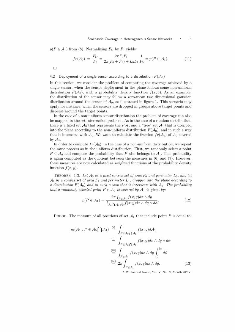
4.2 Deployment of a single sensor according to a distribution F (A0)

In this section, we consider the problem of computing the coverage achieved by asingle sensor, when the sensor deployment in the plane follows some non-uniformdistribution F (A0), with a probability density function f(x, y). As an example,the distribution of the sensor may follow a zero-mean two dimensional gaussiandistribution around the center of A0, as illustrated in figure 1. This scenario mayapply for instance, when the sensors are dropped in groups above target points anddisperse around the target points.

In the case of a non-uniform sensor distribution the problem of coverage can alsobe mapped to the set intersection problem. As in the case of a random distribution,there is a fixed set A0 that represents the FoI, and a “free” set A1 that is droppedinto the plane according to the non-uniform distribution F (A0), and in such a waythat it intersects with A0. We want to calculate the fraction fr(A0) of A0 coveredby A1.

In order to compute fr(A0), in the case of a non-uniform distribution, we repeatthe same process as in the uniform distribution. First, we randomly select a pointP ∈ A0 and compute the probability that P also belongs to A1. This probabilityis again computed as the quotient between the measures in (6) and (7). However,these measures are now calculated as weighted functions of the probability densityfunction f(x, y).

Theorem 4.3. Let A0 be a fixed convex set of area F0 and perimeter L0, and letA1 be a convex set of area F1 and perimeter L1, dropped into the plane according toa distribution F (A0) and in such a way that it intersects with A0. The probabilitythat a randomly selected point P ∈ A0 is covered by A1 is given by:

p(P ∈ A1) =2π

∫P∈A1

f(x, y)dx ∧ dy∫A0TA1 6=∅ f(x, y)dx ∧ dy ∧ dφ

. (12)

Proof. The measure of all positions of set A1 that include point P is equal to:

m(A1 : P ∈ A0

⋂A1)

(i)=

∫

P∈A0TA1

f(x, y)dA1

(ii)=

∫

P∈A0TA1

f(x, y)dx ∧ dy ∧ dφ

(iii)=

∫

P∈A1

f(x, y)dx ∧ dy

∫ 2π

0

dφ

(iv)= 2π

∫

P∈A1

f(x, y)dx ∧ dy. (13)



si

Ai

Non covered region

(a) (b)

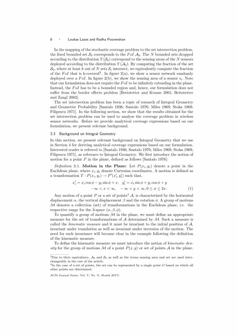
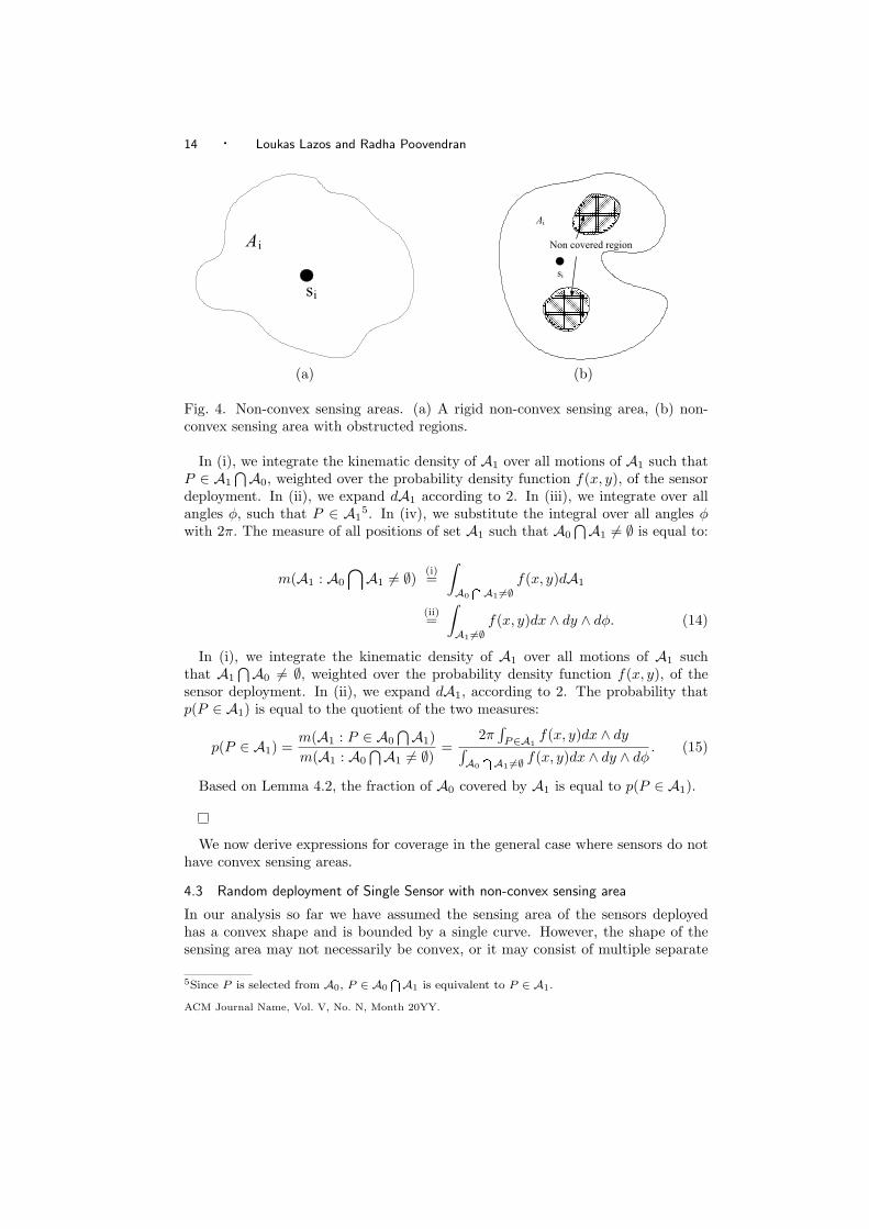
Fig. 4. Non-convex sensing areas. (a) A rigid non-convex sensing area, (b) non-convex sensing area with obstructed regions.

In (i), we integrate the kinematic density of A1 over all motions of A1 such thatP ∈ A1

⋂A0, weighted over the probability density function f(x, y), of the sensordeployment. In (ii), we expand dA1 according to 2. In (iii), we integrate over allangles φ, such that P ∈ A1

5. In (iv), we substitute the integral over all angles φwith 2π. The measure of all positions of set A1 such that A0

⋂A1 6= ∅ is equal to:

m(A1 : A0

⋂A1 6= ∅) (i)

=∫

A0TA1 6=∅

f(x, y)dA1

(ii)=

∫

A1 6=∅f(x, y)dx ∧ dy ∧ dφ. (14)

In (i), we integrate the kinematic density of A1 over all motions of A1 suchthat A1

⋂A0 6= ∅, weighted over the probability density function f(x, y), of thesensor deployment. In (ii), we expand dA1, according to 2. The probability thatp(P ∈ A1) is equal to the quotient of the two measures:

p(P ∈ A1) =m(A1 : P ∈ A0

⋂A1)m(A1 : A0

⋂A1 6= ∅) =2π

∫P∈A1

f(x, y)dx ∧ dy∫A0TA1 6=∅ f(x, y)dx ∧ dy ∧ dφ

. (15)

Based on Lemma 4.2, the fraction of A0 covered by A1 is equal to p(P ∈ A1).

We now derive expressions for coverage in the general case where sensors do nothave convex sensing areas.

4.3 Random deployment of Single Sensor with non-convex sensing area

In our analysis so far we have assumed the sensing area of the sensors deployedhas a convex shape and is bounded by a single curve. However, the shape of thesensing area may not necessarily be convex, or it may consist of multiple separate

5Since P is selected from A0, P ∈ A0TA1 is equivalent to P ∈ A1.



regions due to obstacles, such as walls pillars, trees, etc. In figure 4(i), we showthe a non-convex sensing area bounded by a single curve. In figure 4(ii), we show asensing area with certain areas obstructed by obstacles. Such a non-convex sensingregion is bounded by more than one closed curves. In this section we compute thecoverage achieved by the random deployment of a single sensor with a non-convex6

sensing area.

Theorem 4.4. Let A0 denote the FoI bounded by a simple7 curve, and let A1

denote the sensing area of a sensor si, with A1 being the union of a finite numberof separate convex regions Ai

1, i = 1 . . . m, of total area F1 and total perimeter L1.The probability that a randomly selected point P ∈ A0 is covered by A1 is given by:

p(P ∈ A1) =2πF1

2π(mF0 + F1) + L0L1. (16)

Proof. Theorem 4.4 is a special case of the fundamental kinematic formula ofBlaschke [Blaschke 1955] that measures a group of motions in the plane for thecase where non-convex areas intersect. In Theorem 4.4, the number of separateconvex sets m is defined by the number of closed curves required to bound A1, thatintersect with the FoI. When the sensing area A1 is bounded by a simple curve, asin the case of a compact bounded set, or a convex set, (16) reduces to (5) [Santalo1976] (pp. 116). Detailed proof of Theorem 4.4 is omitted here, but is provided in[Santalo 1976] (pp. 113–118).

Theorem 4.4 allows us to compute the fraction of A0 covered by the deploymentof a single sensor, when the sensing area of the sensor is non-convex, by applyingLemma 4.2. Note that to compute p(P ∈ A1) prior knowledge of a decompositionof the sensing area to a union of disjoint convex areas is required.

4.4 Random Deployment of Multiple Sensors

In this section, we compute the coverage achieved by the random deployment ofN sensors, with each sensor si having a sensing area Ai of size Fi and perimeterLi. As it is implied by our notations, sensors need not have the same sensing areabut can be heterogeneous. We derive formulas for randomly deployed sensors withconvex sensing areas. However, equivalent formulas can be obtained for any otherdistribution and non-convex shapes by using the results of the coverage achievedby a single sensor deployment, derived in Sections 4.2, 4.3.

We initially derive the probability p(S = k) that a randomly selected pointP ∈ A0 is covered by k sensors when N sensors are randomly deployed, using theresults from Section 4.1. We then compute the probability that P ∈ A0 is coveredby at least k sensors, as well as the fraction of A0 covered by at least k sensors.

We then simplify our expressions in the case where the sensing areas are identi-cal, and provide formulas for the unit disk model commonly assumed in coverageproblems [Liu and Towsley 2004; Poduri and Sukhatme 2004]. Finally, we showhow our expressions can be reduced to formulas derived in [Liu and Towsley 2004;

6The boundary of the sensing area must be piecewise twice differentiatable.7A simple curve is defined as a closed curve with no double points [Santalo 1976], pp. 113.



Poduri and Sukhatme 2004] under the assumption that the FoI is infinite and thedeployment density remains constant.

Theorem 4.5. Let N sensors be randomly and independently deployed over aFoI A0, of area F0 and perimeter L0. Let each sensor si have a sensing area Ai ofsize Fi and perimeter Li. The probability p(S = k) that a randomly selected pointP ∈ A0 is covered by exactly k sensors is given by:

p(S = k) =

∏Ni=1

(2πF0+L0Li

2π(F0+Fi)+L0Li

), k = 0P(N

k)i=1 (Qk

j=1(2πFT (i,j))QN−k

z=1 (2πF0+L0LG(i,z)))QNr=1(2π(F0+Fr)+L0Lr)

, k ≥ 1.

(17)

where T is a matrix in which each row j is a “k-choice” of [1 . . . N ] (a vector of kelements out of N), and G is a matrix in which each row j contains the elementsof [1 . . . N ], that do not appear in the jth row of T.

Proof. In order to prove Theorem 4.5, we map the problem of coverage to theset intersection problem, as illustrated in our problem formulation in Section 3.2.Consider first, the case where k = 0. When a single sensor si is deployed, theprobability that it covers a randomly selected point P ∈ A0 is given by Theorem4.1. Hence, the probability p(P /∈ Ai) can be computed as:

p(P /∈ Ai) = 1− p(P ∈ Ai)

= 1− 2πFi

2π(F0 + Fi) + L0Li

=2πF0 + L0Li

2π(F0 + Fi) + L0Li. (18)

Given that fact that the N sensors are independently deployed in the plane so thatthey cover some part ofA0, the probability p(S = 0) that none of theAi, i = 1 . . . Ncovers point P is:

p(S = 0) = p(P /∈ A1, . . . , P /∈ AN )

(i)=

N∏

i=1

p(P /∈ Ai)

(ii)=

N∏

i=1

(2πF0 + L0Li

2π(F0 + Fi) + L0Li

). (19)

Equality in (i) holds due to the independence in the deployment of the sensors si.In (ii), we substitute p(P /∈ Ai) from (18).

In the case where k ≥ 1, we first need to compute the probability that P iscovered by exactly k specific sets. Let T denote a kx

(Nk

)matrix where each row j

is a k-choice of the vector [1 . . . N ], and let G denote a (N−k+1)x(Nk

)matrix where

each row j contains the elements of [1 . . . N ], that do not appear in the jth row ofT. Consider for example, T (1) = [1 . . . k] and G(1) = [k + 1 . . . N ]. The probabilityp(T (1)) that P is covered by exactly the sets with indexes in the first row of T isACM Journal Name, Vol. V, No. N, Month 20YY.


given by:

p(T (1))(i)= p(P ∈ A1, . . . , P ∈ Ak, P /∈ Ak+1, . . . , P /∈ AN )(ii)= p(P ∈ A1), . . . , p(P ∈ Ak)p(P /∈ Ak+1), . . . , p(P /∈ AN )(iii)=

2πF1

2π(F0 + F1) + L0L1. . .

2πFk

2π(F0 + Fk) + L0Lk

2πF0 + L0Lk+1

2π(F0 + Fk+1) + L0Lk+1. . .

2πF0 + L0LN

2π(F0 + FN ) + L0LN

=

∏kj=1(2πFi)

∏Nz=k+1(2πF0 + L0Lz)∏N

r=1 (2π(F0 + Fr) + L0Lr)

=

∏kj=1

(2πFT (1,j)

) ∏N−kz=1

(2πF0 + L0LG(1,z)

)∏N

r=1 (2π(F0 + Fr) + L0Lr). (20)

In (i), we show which k sets include point P. Due to the independence in the setdeployment, in (ii), the intersection of the events in (i) becomes a product of theindividual events. In (iii), we substitute the individual probabilities from (8), (18).In the general case, the probability that the sets with indexes of the ith row of Tcover point P is given by:

p(T (i)) =

∏kj=1

(2πFT (i,j)

) ∏N−kz=1

(2πF0 + L0LG(i,z)

)∏N

r=1 (2π(F0 + Fr) + L0Lr). (21)

Since we are not interested in a specific choice of sets to cover point P, theprobability that p(S = k) is a summation of p(T (i)) for all possible k-choices.Summing p(T (i)) over all i yields (17):

p(S = k) =(N

k)∑

i=1

p(T (i))

=(N

k)∑

i=1

(∏kj=1

(2πFT (i,j)

)∏N−kz=1

(2πF0 + L0LG(i,z)

)∏N

r=1 (2π(F0 + Fr) + L0Lr)

)

=

∑(Nk)

i=1

(∏kj=1

(2πFT (i,j)

) ∏N−kz=1

(2πF0 + L0LG(i,z)

))

∏Nr=1 (2π(F0 + Fr) + L0Lr)

. (22)

Once we have computed p(S = k), we can derive the probability that the ran-domly selected point P is covered by at least k sensors.

Lemma 4.6. Let A0 be a FoI of size F0 and perimeter L0, and let N sensorswith sensing area Ai of size Fi and perimeter Li be independently and randomlydeployed over A0. The probability that a randomly selected point of A0 is covered



by at least k sensors is given by:

p(S ≥ k) =

1 k = 0,

1−∑k−1l=0

P(Nl )

i=1 (Qlj=1(2πFT (i,j))

QN−lz=1 (2πF0+L0LG(i,z)))QN

r=1(2π(F0+Fr)+L0Lr)k ≥ 1.

(23)

Proof. Lemma 4.6, holds by observing:

p(S ≥ k) = 1−k−1∑

l=0

p(l = i), (24)

and substituting (17) to (24).

Lemma 4.6, allows us to compute the fraction fr(A0) covered by at least k sets.

Theorem 4.7. The fraction fr(A0) of a FoI A0 of area F0 and perimeter L0

that is covered by at least k sensors when N sensors of sensing area Ai of size Fi

and perimeter Li, are randomly and independently deployed in the plane in such away that they cover some part of the FoI is given by:

fr(A0) =

1 k = 0,

1−∑k−1l=0

P(Nl )

i=1 (Qlj=1(2πFT (i,j))

QN−lz=1 (2πF0+L0LG(i,z)))QN

r=1(2π(F0+Fr)+L0Lr)k ≥ 1.

(25)

Proof. By mapping the coverage problem to the set intersection problem, thesize FC of the area covered by at least k sensors can be computed by integratingthe probability that a randomly selected point P ∈ A0 is covered by at least k sets,over all points P :

FC =∫

P∈A0

p(S ≥ k)dP = p(P ≥ k)∫

P∈A0

dP = p(P ≥ k)F0. (26)

Normalizing FC by F0 yields the result of Theorem 4.7.

The fraction fr(A0) covered by at least k sensors is equal to the probability thata randomly selected point P is covered by at least k sensors.

Corollary 4.8. The fraction of A0 that is not covered by any sensor when Nsensors are randomly deployed is given by:

p(S = 0) =N∏

i=1

(2πF0 + L0Li

2π(F0 + Fi) + L0Li

). (27)

Proof. The Corollary follows from Theorem 4.5, for k = 0.

4.5 Coverage in the case of Homogeneous Sensing Areas

The analytic expressions derived in Section 4.4 hold for heterogeneous sensor net-works where the sensing areas of the sensors are of different size and perimeter.In the case of homogeneous sensor networks where for each sensor si, i = 1 . . . NFi = F and Li = L, the coverage expressions can be simplified to expressionsinvolving binomials.ACM Journal Name, Vol. V, No. N, Month 20YY.


Corollary 4.9. The fraction fr(A0) of a FoI A0 of area F0 and perimeterL0 that is covered by at least k sensors when N sensors of sensing area Ai of sizeFi = F and perimeter Li = L are randomly and independently deployed in the planein such a way that they cover some part of FoI is given by:

fr(A0) =

1 k = 0,

1−∑k−1l=0

((N

l )(2πF )l(2πF0+L0L)N−l

(2π(F0+F )+L0L)N

)k ≥ 1.

(28)

Proof. The corollary holds by substituting FT (i,j) = F, LG(i,j) = L in (25).

Note that so far in our computations, the FoI is a bounded region. Previousanalytical results for homogeneous sensor networks require that the FoI of interestis infinitely expanding in the plane [Liu and Towsley 2004; Poduri and Sukhatme2004, Miorandi and Altman 2005], and provide asymptotic formulas of coverage.Under the same assumption and using Corollary 4.9, we can derive the same as-ymptotic results expressed in the following Corollary.

Corollary 4.10. Let N sensors of sensing area Ai of size Fi = F and perime-ter Li = L be randomly and independently deployed in the plane, in such a waythat they cover some part of a FoI A0 of size F0 and perimeter L0. If A0 expandsin the whole plane in such a way such that the sensor density remains a constant( N

F0→ ρ), the fraction fr(A0) covered by at least k sensors is given by:

fr(A0) →{

1 k = 0,

1−∑k−1l=0

((ρF )l

k! e−ρF)

, k ≥ 1.(29)

Proof. Let us first compute the probability that exactly k sets intersect in arandomly selected point P ∈ A0. Substituting Fi = F, Li = L in (17) yields:

p(S = k) =(

N

k

)(2πF

2π(F0 + F ) + L0L

)k (2πF0 + L0L

2π(F0 + F ) + L0L

)N−k

=(

N

k

)qk (1− q)N−k

, (30)

where q = 2πF2π(F0+F )+L0L . The binomial distribution can be approximated by a

Poisson distribution when N goes to infinity:

limN→∞

p(S = k) =(Nq)k

k!e−Nq. (31)

As F0 → ∞, FF0

→ 0 and if the sensor deployment density NF0

→ ρ where ρ isconstant, Nq asymptotically tends to:

limF0→∞, N

F0→ρ

(Nq) = limF0→∞, N

F0→ρ

(2πNF

2π(F0 + F ) + L0L

)

= limF0→∞, N

F0→ρ

2πNF

2πF0

(1 + F

F0+ L0L

2πF0

)

=NF

F0= ρF, (32)



since L0F0→ 0 regardless of the shape of A0 [Santalo 1976]. Substituting (32) into

(31), yields:

p(S = k) → (Nq)k

k!e−Nq =

(N FF0

)k

k!e−N F

F0 =(ρF )k

k!e−ρF . (33)

Hence, the fraction fr(A0) of A0 covered by at least k sensors with identical sensingarea Ai, when sensors are deployed randomly with a constant density ρ, as A0

expands in the whole plane is given by:

limN→∞

fr(A0) = limN→∞

(1−

k−1∑

l=0

p(S = k)

)

= 1− limN→∞

(k−1∑

l=0

p(S = k)

)= 1−

k−1∑

l=0

(lim

N→∞p(S = k)

)

=

{1 k = 0,

1−∑k−1l=0

((ρF )l

l! e−ρF)

, k ≥ 1.(34)

We now validate our theoretical results via simulation.

5. VALIDATION OF THE THEORETICAL RESULTS

In this section, we validate our theoretical results via simulation. We also compareour results with the approximation formulas derived in [Liu and Towsley 2004;Poduri and Sukhatme 2004, Miorandi and Altman 2005]. Our evaluation is donein terms of the Kullback Leibler distance (KL-distance) of the probability densityfunctions (pdfs), which provides a performance comparison in the average sense.Considering the pdf obtained via simulation to be the desired distribution q, wecompute the KL-distance of our theoretical formulas and the approximations pro-vided in [Liu and Towsley 2004; Poduri and Sukhatme 2004, Miorandi and Altman2005]. The KL-distance for two distributions p, q, when q is the desired distributionand p is the true distribution is defined as follows [Cover and Thomas 1991],

Definition 5.1. Kullback Leibler distance–The Kullback Leibler distance betweena desired distribution q and a true distribution p is equal to:

KL(p, q) =∑pi

pi log2

pi

qi, (35)

where pi, qi denote the discrete values of the distributions p, q respectively.

We also compare theory, simulation and approximation results with respect tothe total variation distance (TV-distance), a metric that reflects the worst caseperformance and is defined as follows.

Definition 5.2. Total variation distance–The total variation distance betweentwo distributions q, p is the maximum difference between the probabilities that canbe assigned to the same event,

TV (p, q) = supi{|pi − qi|}. (36)



100 200 300 400 500

0.2

0.4

0.6

0.8

Non−covered Fraction of A0

Sensors deployed (N)

Fra

ctio

n fr

(A0)

TheoreticalPoisson AppxSimulated

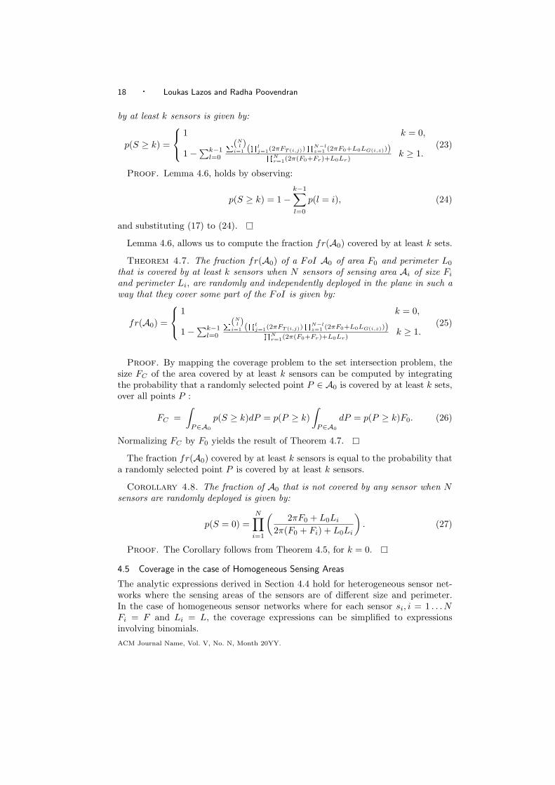
Fig. 5. Fraction fr(A0) of A0, that remains non-covered as a function of the numberof sensors N that are deployed to monitor the FoI.

We validate our formulas for homogeneous networks (sensors have identical sensingarea) as well as heterogeneous networks (sensors have different sensing areas).

5.1 Homogeneous Sensor Network- Unit Disk Sensing Area

In our first experiment, we randomly deployed a variable number of sensors withidentical sensing area in a circular FoI of radius R = 100m. All sensors had acircular sensing area of radius r = 10m. We repeated the random deployment ofsensors 100 times and averaged the results. In figure 5(a), we show the fractionfr(A0) of A0, that remains non-covered as a function of the number of sensors Nthat are deployed to monitor the FoI. The theoretical formula that computes thatdesired fraction is obtained from Corollary 4.8 and is equal to:

fr(A0) = p(S = 0) =N∏

i=1

2πF0 + L0Li

2π(F0 + Fi) + L0Li=

N∏

i=1

2πF0 + L0L

2π(F0 + F ) + L0L

=(

2πF0 + L0L

2π(F0 + F ) + L0L

)N

,(37)

where F0 = πR2, L0 = 2πR, F = πr2, L = 2πr. The Poisson approximation of thefraction of A0 that is non-covered is given by [Liu and Towsley 2004; Poduri andSukhatme 2004, Miorandi and Altman 2005]:

fr′(A0) = p′(S = 0) = e−NFF0 . (38)

We observe that the simulation results verify our theoretical expression, while thePoisson approximation deviates from the simulation results. In figure 6(a), we showthe pdf of the fraction fr(A0) covered by exactly k sensors when N = 300 sensorswith identical sensing area are randomly deployed. The equivalent sensor densityis equal to ρ = 0.0095 sensors/m2. The same graphs for N = 500, N = 1, 000(densities ρ = 0.016 sensors/m2, ρ = 0.032 sensors/m2) are provided in figures 6(c)and 7(a), respectively. According to Theorem 4.7, fr(A0) is equal to the pdf of theprobability that a randomly selected point P is covered by exactly k sensors. Our



0 2 4 6 8 10 12 140

0.05

0.1

0.15

0.2

0.25

k (sensors)

Fra

ctio

n f

r(A

0)

TheoreticalPoisson Appx

Simulated

0 2 4 6 8 10 12 140

0.1

0.2

0.3

0.4

0.5

0.6

0.7

0.8

0.9

k (sensors)

Fra

ction fr(

A0)

Fraction of A0

TheoreticalPoisson Appx

Simulated

(a) (b)

0 5 10

0.05

0.1

0.15

Probability density function p(S=k) for N=500

k (sensors)

Fra

ctio

n fr

(A0)


0 2 4 6 8 10 12 14

0.2

0.4

0.6

0.8

Fraction of A0 covered by at least k sensors for N=500

k (sensors)

Fra

ctio

n fr

(A0)


(c) (d)

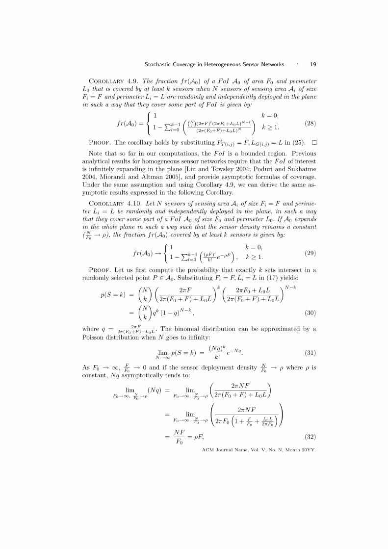
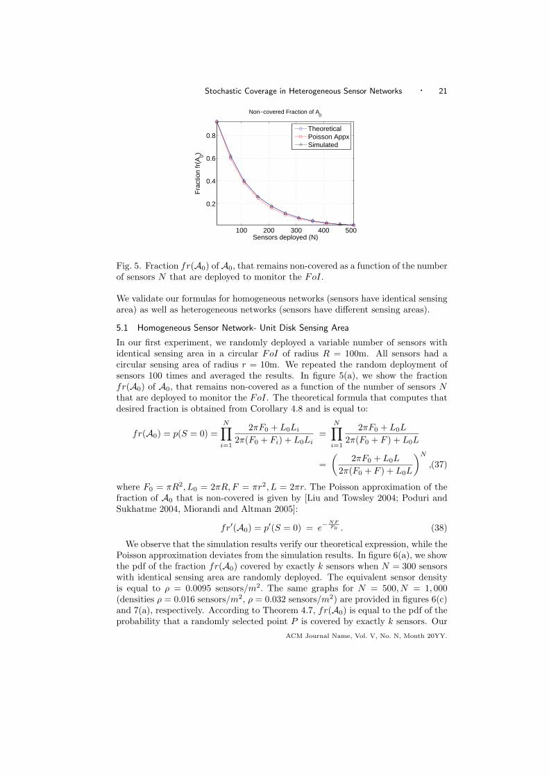
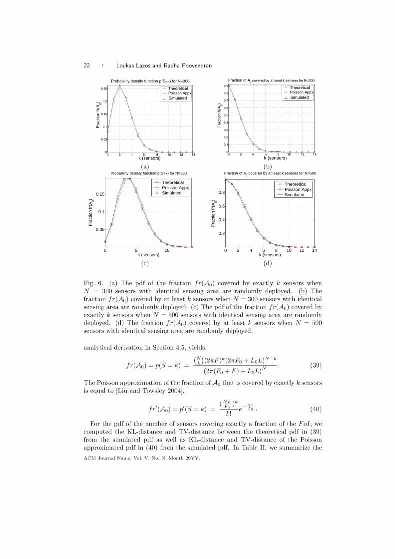
Fig. 6. (a) The pdf of the fraction fr(A0) covered by exactly k sensors whenN = 300 sensors with identical sensing area are randomly deployed. (b) Thefraction fr(A0) covered by at least k sensors when N = 300 sensors with identicalsensing area are randomly deployed. (c) The pdf of the fraction fr(A0) covered byexactly k sensors when N = 500 sensors with identical sensing area are randomlydeployed. (d) The fraction fr(A0) covered by at least k sensors when N = 500sensors with identical sensing area are randomly deployed.

analytical derivation in Section 4.5, yields:

fr(A0) = p(S = k) =

(Nk

)(2πF )k(2πF0 + L0L)N−k

(2π(F0 + F ) + L0L)N. (39)

The Poisson approximation of the fraction of A0 that is covered by exactly k sensorsis equal to [Liu and Towsley 2004],

fr′(A0) = p′(S = k) =(NF

F0)k

k!e−

NFF0 . (40)

For the pdf of the number of sensors covering exactly a fraction of the FoI, wecomputed the KL-distance and TV-distance between the theoretical pdf in (39)from the simulated pdf as well as KL-distance and TV-distance of the Poissonapproximated pdf in (40) from the simulated pdf. In Table II, we summarize theACM Journal Name, Vol. V, No. N, Month 20YY.


0 5 10 15 20

0.02

0.04

0.06

0.08

0.1

0.12

0.14


k (sensors)

Fra

ctio

n fr

(A0)


0 5 10 15 20

0.2

0.4

0.6

0.8


k (sensors)

Fra

ctio

n fr

(A0)


(a) (b)

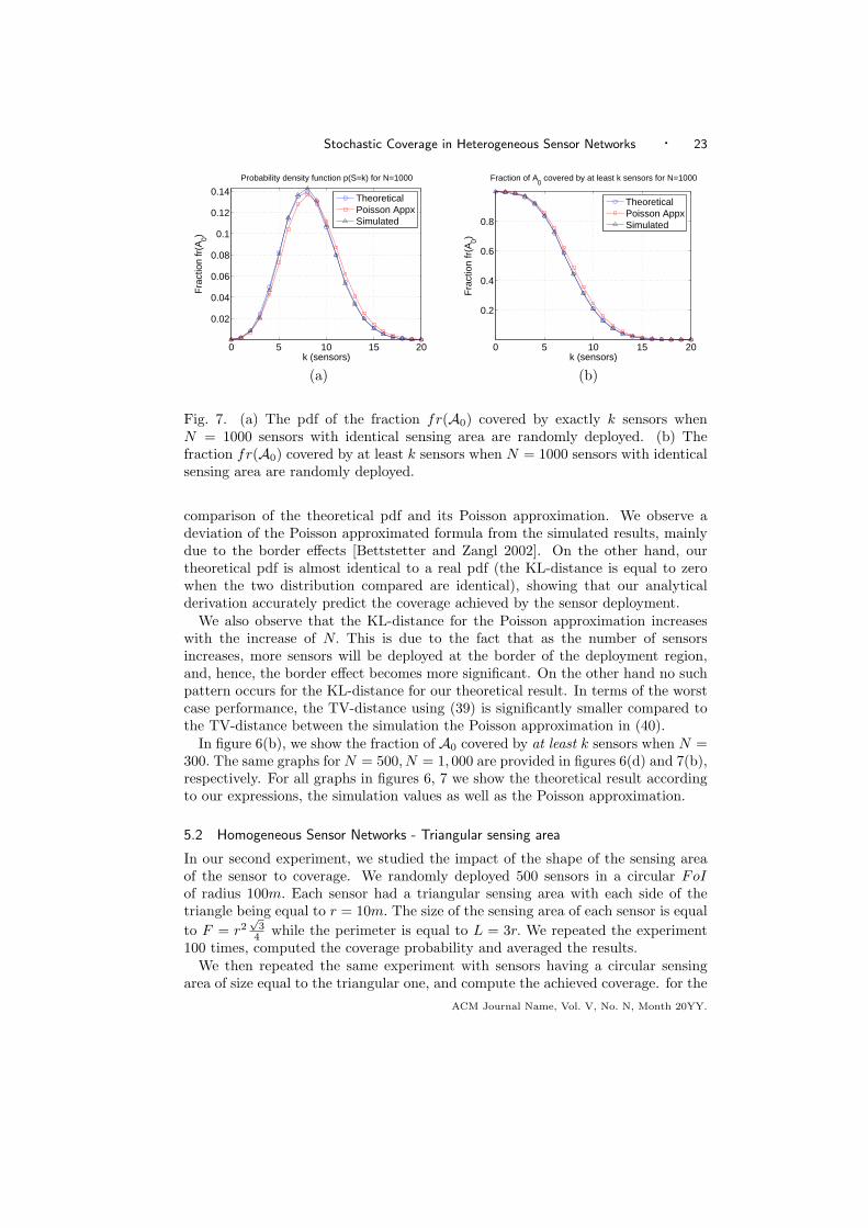
Fig. 7. (a) The pdf of the fraction fr(A0) covered by exactly k sensors whenN = 1000 sensors with identical sensing area are randomly deployed. (b) Thefraction fr(A0) covered by at least k sensors when N = 1000 sensors with identicalsensing area are randomly deployed.

comparison of the theoretical pdf and its Poisson approximation. We observe adeviation of the Poisson approximated formula from the simulated results, mainlydue to the border effects [Bettstetter and Zangl 2002]. On the other hand, ourtheoretical pdf is almost identical to a real pdf (the KL-distance is equal to zerowhen the two distribution compared are identical), showing that our analyticalderivation accurately predict the coverage achieved by the sensor deployment.

We also observe that the KL-distance for the Poisson approximation increaseswith the increase of N. This is due to the fact that as the number of sensorsincreases, more sensors will be deployed at the border of the deployment region,and, hence, the border effect becomes more significant. On the other hand no suchpattern occurs for the KL-distance for our theoretical result. In terms of the worstcase performance, the TV-distance using (39) is significantly smaller compared tothe TV-distance between the simulation the Poisson approximation in (40).

In figure 6(b), we show the fraction of A0 covered by at least k sensors when N =300. The same graphs for N = 500, N = 1, 000 are provided in figures 6(d) and 7(b),respectively. For all graphs in figures 6, 7 we show the theoretical result accordingto our expressions, the simulation values as well as the Poisson approximation.

5.2 Homogeneous Sensor Networks - Triangular sensing area

In our second experiment, we studied the impact of the shape of the sensing areaof the sensor to coverage. We randomly deployed 500 sensors in a circular FoIof radius 100m. Each sensor had a triangular sensing area with each side of thetriangle being equal to r = 10m. The size of the sensing area of each sensor is equalto F = r2

√3

4 while the perimeter is equal to L = 3r. We repeated the experiment100 times, computed the coverage probability and averaged the results.

We then repeated the same experiment with sensors having a circular sensingarea of size equal to the triangular one, and compute the achieved coverage. for the



Theoretical Result in (39) Poisson Approximation in (40)

Number of Nodes (N) KL dist. TV dist. KL dist. TV dist.(x10−3) (x10−3) (x10−3) (x10−3)

300 0.56 14.3 4.2 34.4

500 0.11 6.4 5.9 58.5

700 0.062 4.4 7.1 48.0

1000 0.096 3.6 9.4 52.1

1500 0.01 2.8 13.4 40.6

R = 100m, r = 10m, F0 = πR2, L0 = 2π, F = πr2, L0 = 2πr

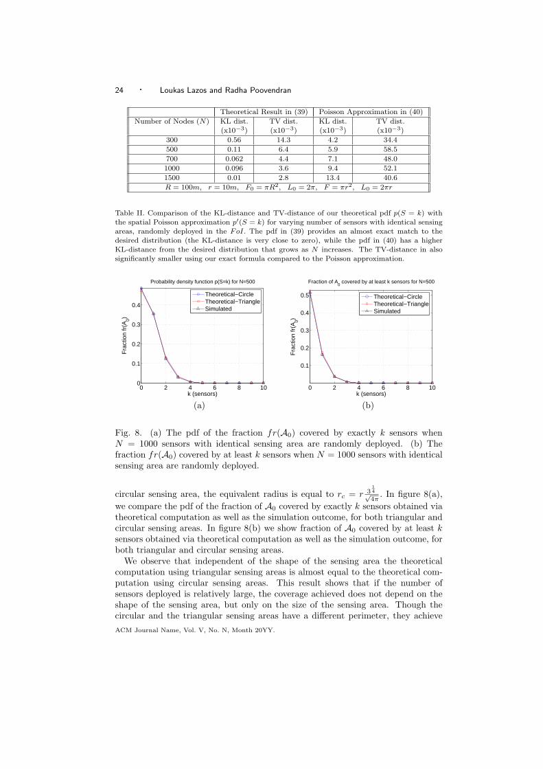
Table II. Comparison of the KL-distance and TV-distance of our theoretical pdf p(S = k) withthe spatial Poisson approximation p′(S = k) for varying number of sensors with identical sensingareas, randomly deployed in the FoI. The pdf in (39) provides an almost exact match to thedesired distribution (the KL-distance is very close to zero), while the pdf in (40) has a higherKL-distance from the desired distribution that grows as N increases. The TV-distance in alsosignificantly smaller using our exact formula compared to the Poisson approximation.

0 2 4 6 8 100

0.1

0.2

0.3

0.4


k (sensors)

Fra

ctio

n fr

(A0)

Theoretical−CircleTheoretical−TriangleSimulated

0 2 4 6 8 10

0.1

0.2

0.3

0.4

0.5


k (sensors)

Fra

ctio

n fr

(A0)

Theoretical−CircleTheoretical−TriangleSimulated

(a) (b)

Fig. 8. (a) The pdf of the fraction fr(A0) covered by exactly k sensors whenN = 1000 sensors with identical sensing area are randomly deployed. (b) Thefraction fr(A0) covered by at least k sensors when N = 1000 sensors with identicalsensing area are randomly deployed.

circular sensing area, the equivalent radius is equal to rc = r 314√4π

. In figure 8(a),we compare the pdf of the fraction of A0 covered by exactly k sensors obtained viatheoretical computation as well as the simulation outcome, for both triangular andcircular sensing areas. In figure 8(b) we show fraction of A0 covered by at least ksensors obtained via theoretical computation as well as the simulation outcome, forboth triangular and circular sensing areas.

We observe that independent of the shape of the sensing area the theoreticalcomputation using triangular sensing areas is almost equal to the theoretical com-putation using circular sensing areas. This result shows that if the number ofsensors deployed is relatively large, the coverage achieved does not depend on theshape of the sensing area, but only on the size of the sensing area. Though thecircular and the triangular sensing areas have a different perimeter, they achieveACM Journal Name, Vol. V, No. N, Month 20YY.


the same coverage since they have the same size F.Analyzing formula (23), the coverage probability depends on the fractions F

F0, L0L

F0.

Since in our experiment the triangular sensing area had the same size as the circu-lar sensing area the difference in the coverage probability in the two deploymentsdepends only on the fraction L0L

F0. However, the difference in the fraction L0L

F0for

triangles and circles is negligible with respect to the value of 2π, or(2π + F

F0

)where

it is added. Hence, although A0 does not extend infinitely, its size is sufficientlylarge such that the impact of the perimeter of the sensing area L is negligible. Thiswould not be the case if F0 and L where of comparable size, or the perimeters ofthe sensing areas differed significantly.

The independence of the coverage achieved from the shape of the sensing areas,is also illustrated in the Poisson approximation shown in (31), where the coverageonly depends on the size of the area F and not the perimeter L. As F0 increasesboth L

F0and L0

F0tend to zero [Santalo 1976] and, hence, the perimeter of both the

FoI and the sensing area do not influence the coverage probability.

5.3 Heterogeneous Sensor Networks

In our second experiment, we considered a hierarchical (heterogeneous) sensor net-work, where two types of sensors are deployed. Type A has a sensing area of diskshape with a sensing range rA = 10m, while type B has a sensing area of diskshape with a sensing range of rB = 15m. We randomly deployed an equal num-ber NA = NB = N

2 of sensors of each type over a circular FoI of size F0 = πR2

where R = 100m. In figure 9, we show the fraction fr(A0) of A0, that remainsnon-covered as a function of the number of sensors N that are deployed to monitorthe FoI. The theoretical formula that compute that is equal to:

fr(A0) = p(S = 0) =N∏

i=1

2πF0 + L0Li

2π(F0 + Fi) + L0Li, (41)

where F0 = πR2, L0 = 2πR, Fi = πr2i , L = 2πri. The Poisson approximation of the

fraction of A0 that is non-covered was illustrated in [Miorandi and Altman 2005],and is given by,

fr′(A0) = p′(S = 0) = e−NE[F ]

F0 . (42)

where E[F ] = πE[r2] denotes the expected value of the sensing area of the sensorsdeployed.

We observe that the simulation results verify our theoretical expression, whilethe Poisson approximation deviates from the simulation results. In figure 10(a), weshow the pdf of the fraction fr(A0) covered by exactly k sensors when N = 300sensors are randomly deployed. The equivalent sensor density is equal to ρ = 0.0095sensors/m2. The same graphs for N = 500, N = 1, 000 (densities ρ = 0.016sensors/m2, ρ = 0.032 sensors/m2) are provided in figures 10(c) and 11(a), re-spectively. According to Theorem 4.7, fr(A0) is equal to the pdf p(S = k) of theprobability that a randomly selected point P is covered by exactly k sensors. Our



0 100 200 300 400 5000

0.2

0.4

0.6

0.8

1Non-covered Fraction of A

0for variable r

Sensors deployed (N)

Fra

ction fr(

A0)

Theoretical

Poisson Appx

Simulated

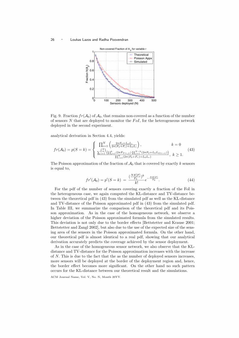
Fig. 9. Fraction fr(A0) of A0, that remains non-covered as a function of the numberof sensors N that are deployed to monitor the FoI, for the heterogeneous networkdeployed in the second experiment.

analytical derivation in Section 4.4, yields:

fr(A0) = p(S = k) =

∏Ni=1

(2πF0+L0Li

2π(F0+Fi)+L0Li

), k = 0P(N

k)i=1 (Qk

j=1(2πFT (i,j))QN−k

z=1 (2πF0+L0LG(i,z)))QNr=1(2π(F0+Fr)+L0Lr)

, k ≥ 1.

(43)

The Poisson approximation of the fraction of A0 that is covered by exactly k sensorsis equal to,

fr′(A0) = p′(S = k) =(NE[F ]

F0)k

k!e−

NE[F ]F0 . (44)

For the pdf of the number of sensors covering exactly a fraction of the FoI inthe heterogeneous case, we again computed the KL-distance and TV-distance be-tween the theoretical pdf in (43) from the simulated pdf as well as the KL-distanceand TV-distance of the Poisson approximated pdf in (43) from the simulated pdf.In Table III, we summarize the comparison of the theoretical pdf and its Pois-son approximation. As in the case of the homogeneous network, we observe ahigher deviation of the Poisson approximated formula from the simulated results.This deviation is not only due to the border effects [Bettstetter and Krause 2001;Bettstetter and Zangl 2002], but also due to the use of the expected size of the sens-ing area of the sensors in the Poisson approximated formula. On the other hand,our theoretical pdf is almost identical to a real pdf, showing that our analyticalderivation accurately predicts the coverage achieved by the sensor deployment.

As in the case of the homogeneous sensor network, we also observe that the KL-distance and TV-distance for the Poisson approximation increases with the increaseof N. This is due to the fact that the as the number of deployed sensors increases,more sensors will be deployed at the border of the deployment region and, hence,the border effect becomes more significant. On the other hand no such patternoccurs for the KL-distance between our theoretical result and the simulations.ACM Journal Name, Vol. V, No. N, Month 20YY.


0 5 10

0.05

0.1

0.15

Pdf p(S=k) for N=300 and heterogeneous network

k (sensors)

Fra

ctio

n fr

(A0)


0 2 4 6 8 10 12 14

0.2

0.4

0.6

0.8

fr(A0) covered by at least k sensors for N=300

k (sensors)

Fra

ctio

n fr

(A0)


(a) (b)

0 5 10 15 200

0.05

0.1

0.15


k (sensors)

Fra

ctio

n fr

(A0)


0 5 10 15 20

0.2

0.4

0.6

0.8


k (sensors)

Fra

ctio

n fr

(A0)


(c) (d)

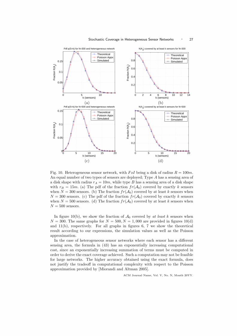
Fig. 10. Heterogeneous sensor network, with FoI being a disk of radius R = 100m.An equal number of two types of sensors are deployed; Type A has a sensing area ofa disk shape with radius rA = 10m, while type B has a sensing area of a disk shapewith rB = 15m. (a) The pdf of the fraction fr(A0) covered by exactly k sensorswhen N = 300 sensors. (b) The fraction fr(A0) covered by at least k sensors whenN = 300 sensors. (c) The pdf of the fraction fr(A0) covered by exactly k sensorswhen N = 500 sensors. (d) The fraction fr(A0) covered by at least k sensors whenN = 500 sensors.

In figure 10(b), we show the fraction of A0 covered by at least k sensors whenN = 300. The same graphs for N = 500, N = 1, 000 are provided in figures 10(d)and 11(b), respectively. For all graphs in figures 6, 7 we show the theoreticalresult according to our expressions, the simulation values as well as the Poissonapproximation.

In the case of heterogeneous sensor networks where each sensor has a differentsensing area, the formula in (43) has an exponentially increasing computationalcost, since an exponentially increasing summation of terms must be computed inorder to derive the exact coverage achieved. Such a computation may not be feasiblefor large networks. The higher accuracy obtained using the exact formula, doesnot justify the tradeoff in computational complexity with respect to the Poissonapproximation provided by [Miorandi and Altman 2005].



0 10 20 300

0.02

0.04

0.06

0.08

0.1


k (sensors)

Fra

ctio

n fr

(A0)


0 5 10 15 20 25 30

0.2

0.4

0.6

0.8

1


k (sensors)

Fra

ctio

n fr

(A0)


(a) (b)Fig. 11. Heterogeneous sensor network, with FoI being a disk of radius R = 100m.An equal number of two types of sensors are deployed; Type A has a sensing areaof a disk shape with radius rA = 10m, while type B has a sensing area of a diskshape with rB = 15m. (a) The pdf of the fraction fr(A0) covered by exactly ksensors when N = 1000 sensors. (b) The fraction fr(A0) covered by at least ksensors when N = 1000 sensors.

Theoretical Result in (43) Poisson Approximation in (44)

Number of Nodes (N) KL dist. TV dist. KL dist. TV dist.(x10−3) (x10−3) (x10−3) (x10−3)

300 0.86 14.7 2.2 36.3

500 1.4 18.3 6.9 38.4

700 0.062 7.8 8.4 49.4

1000 0.096 10.9 12.3 59.6

1500 0.15 11.5 15.7 65.2

R = 100m, rA = 10m, rB = 15m, F0 = πR2, L0 = 2π

FA = πr2A, LA = 2πrA, FB = πr2

B , LB = 2πrB , NA = NB = N2

Table III. Heterogeneous sensor network, with FoI being a disk of radius R = 100m. An equalnumber of two types of sensors are deployed; Type A has a sensing area of a disk shape withradius rA = 10m, while type B has a sensing area of a disk shape with rB = 15m. The tablecompares the KL-distance and TV-distance of our theoretical pdf p(S = k) with the spatial Poissonapproximation p′(S = k) for varying number of sensors with identical sensing areas, randomlydeployed in the FoI. The pdf in (43) provides an almost exact match to the desired distribution(the KL-distance is very close to zero), while the pdf in (44) has a significant distance from thedesired distribution that grows as N increases.

In such a case, a similar approximation can be used for our formulas by employingthe expressions derived for a homogeneous sensor network and substituting the sizeF and perimeter L of the sensing area of the sensors with the expected size E[F ]and expected perimeter E[L]. The theoretical approximation for such a case is:

fr(A0) = p(S = k) =

(Nk

)(2πE[F ])k(2πF0 + L0E[L])N−k

(2π(F0 + E[F ]) + L0E[L])N. (45)

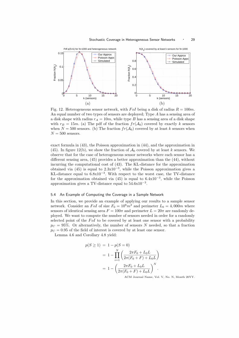
In figure 12(a) we show the pdf obtained via simulation for our heterogeneoussensor network experiment, for N = 500 sensors, the theoretical values based on theACM Journal Name, Vol. V, No. N, Month 20YY.


0 5 10 15 200

0.05

0.1

0.15


k (sensors)

Fra

ctio

n fr

(A0)

Our ApproxPoisson AppxSimulated

0 5 10 15 200

0.2

0.4

0.6

0.8


k (sensors)

Fra

ctio

n fr

(A0)

Our ApproxPoisson AppxSimulated

(a) (b)Fig. 12. Heterogeneous sensor network, with FoI being a disk of radius R = 100m.An equal number of two types of sensors are deployed; Type A has a sensing area ofa disk shape with radius rA = 10m, while type B has a sensing area of a disk shapewith rB = 15m. (a) The pdf of the fraction fr(A0) covered by exactly k sensorswhen N = 500 sensors. (b) The fraction fr(A0) covered by at least k sensors whenN = 500 sensors.

exact formula in (43), the Poisson approximation in (44), and the approximation in(45). In figure 12(b), we show the fraction of A0 covered by at least k sensors. Weobserve that for the case of heterogeneous sensor networks where each sensor has adifferent sensing area, (45) provides a better approximation than the (44), withoutincurring the computational cost of (43). The KL-distance for the approximationobtained via (45) is equal to 2.3x10−3, while the Poisson approximation gives aKL-distance equal to 6.8x10−3. With respect to the worst case, the TV-distancefor the approximation obtained via (45) is equal to 6.4x10−3, while the Poissonapproximation gives a TV-distance equal to 54.6x10−3.

5.4 An Example of Computing the Coverage in a Sample Network

In this section, we provide an example of applying our results to a sample sensornetwork. Consider an FoI of size F0 = 106m2 and perimeter L0 = 4, 000m wheresensors of identical sensing area F = 100π and perimeter L = 20π are randomly de-ployed. We want to compute the number of sensors needed in order for a randomlyselected point of the FoI to be covered by at least one sensor with a probabilitypC = 95%. Or alternatively, the number of sensors N needed, so that a fractionpC = 0.95 of the field of interest is covered by at least one sensor.

Lemma 4.6 and Corollary 4.8 yield:

p(S ≥ 1) = 1− p(S = 0)

= 1−N∏

i=1

(2πF0 + L0L

2π(F0 + F ) + L0L

)

= 1−(

2πF0 + L0L

2π(F0 + F ) + L0L

)N

.



We want to the probability of 1-coverage to be at least p(S ≥ 1) ≥ p. Hence,

P (S ≥ 1) = 1−(

2πF0 + L0L

2π(F0 + F ) + L0L

)N

≥ pC ⇒

N ≥ log (1− pC)

log(

2πF0+L0L2π(F0+F )+L0L

) .

Substituting the values for pC , F0, L0, F, L yields N ≥ 9, 728 sensors.

6. CONCLUSION

We studied the problem of stochastic coverage in heterogeneous sensor networks. Bymapping the coverage problem to the set intersection problem, we derived analyticalformulas that compute the k-coverage when sensors are deployed in a Field ofInterest according to an arbitrary distribution Y. In our analysis, the sensors canhave a sensing area of any shape and also need not have identical sensing areas.We provided simplified expressions for the case when the sensors are randomlydeployed, as well as when the sensors have identical sensing areas.

We verified our theoretical results via simulation and compared them with previ-ous formulas that characterized coverage in both homogeneous and heterogeneoussensor networks. By evaluating the KL-distance between the analytic coverage for-mulas and the simulation, we showed that our expressions provide a significantlyhigher accuracy. This is due to the fact that our results do not suffer from the bor-der effects and hold exactly rather than approximately. We also provided exampleson how to utilize our expressions in order to compute the number of sensors thatneed to be deployed in a Field of Interest, so that a coverage requirement is met.

APPENDIX

1. MEASURE OF ALL MOTIONS OF A1 SUCH THAT IT INTERSECTS WITH A0

In this section, we compute the measure of all motions ofA1 such thatA0

⋂A1 6= 0 :

m(A1 : A0

⋂A1 6= ∅) (i)

=∫

A0TA1 6=∅

dA1

(ii)=

∫

A0TA1 6=∅

dx ∧ dy ∧ dφ

(iii)=

∫ 2π

0

(F0 + F1 + 2F01) dφ

(iv)= 2π(F0 + F1) + L0L1. (46)

In (i), we integrate the kinematic density dA1 of set A1 over all motions of A1

such that A0

⋂A1 6= ∅. In (ii), we write the kinematic density in its expandeddifferential form as defined in (2). In (iii), we compute the area between A0,A1

which is called mixed area of Minkowski and integrate over all possible rotations.The integration yields the desired result.ACM Journal Name, Vol. V, No. N, Month 20YY.


1.1 Proof of (iii)

The proof is due to [Santalo 1936; Santalo 1976]. LetA0,A1 be two convex sets withsupport functions p0(φ), p1(φ), respectively. The support function p(φ) of a convexset A denotes the distance of the origin point of a convex set from the envelopethat defines the curve that bounds the convex set, as a function of the angle φ ofthe envelope with the x-axis of the coordinate system. Let A0,A1 intersect and letA01 denote the common area between A0,A1. A01 is called the mixed convex setof A0,A1, and has a support function p(φ) = p0(φ) + p1(φ).

The area if the mixed convex set can be computed by the decomposition intoelementary triangles of height equal to p and base equal to ds, where ds is theelementary arc of the convex curve that bounds A01 :

F =12

∫

dA01

pds

(i)=

12

∫ 2π

0

p(p + p′′)dφ

(ii)=

12

∫ 2π

0

(p2 − p′2

)dφ

(iii)=

12

∫ 2π

0

((p0 + p1)2 − (p0 + p1)′2

)dφ

=12

∫ 2π

0

(p20 − p′20

)dφ +

12

∫ 2π

0

(p21 − p′21

)dφ +

12

∫ 2π

0

(p0p1 − p′0p′1) dφ

= F0 + F1 + 2F01, (47)

where,

F01 =12

∫ 2π

0

(p0p1 − p′0p′1) . (48)

Equation (i), is due by the definition of the support function [Bonnesen and Fenchel1934; Santalo 1976]. In (ii), we do integration by parts and in (iii) we replacep = p0 + p1.

1.2 Proof of (iv)

In this section, we want to compute the integral:

I =∫ 2π

0

(F0 + F1 + 2F01) dφ. (49)

The computation is as follows:

I =∫ 2π

0

(F0 + F1 + 2F01) dφ

= 2πF0 + 2πF1 +∫ 2π

0

2F01dφ. (50)



F01 =12

∫ 2π

0

(p0p1 − p′0p′1) dφ

(i)=

12

∫ 2π

0

(p0(p1 + p′′1)) dφ

(ii)=

12

∫

dA1

p0ds1

(iii)=

12

∫

dA1

p0(φ− θ)ds1. (51)

Equation (i) is obtained by performing integration by parts. In (ii), we replacep1 +p′′1 , with ds1 ([Bonnesen and Fenchel 1934; Santalo 1976]). In (iii), we considerall possible rotations θ of A1, such that A1, intersects with A0. Integrating, overall θ yields,

∫ (

0

2πF01)(θ)dθ =∫ 2π

0

(12

∫

dA1

p0(φ− θ)ds1

)dθ

=12

∫

dA1

(∫ 2π

0

p0(φ− θ)dθ

)ds1

=12

∫

dA1

L0ds1

=12L0L1, (52)

where we have used the fact that [Santalo 1976]:∫ 2π

0

p0dθ = L0,

∫

dA1

ds1 = L1. (53)

Substituting (52) into (50) yields:

I = 2πF0 + 2πF1 + L0L1. (54)

REFERENCES

Akyildiz, I., Su, W., Sankarasubramaniam, Y., and Cayirci, E. 2002. A survey on sensornetworks. IEEE Communications Magazine 40, 8, 102–114.

Bettstetter, C. and Krause, O. 2001. On border effects in modeling and simulation of wirelessad hoc networks. In Proceedings of the IEEE MWCN ’01.

Bettstetter, C. and Zangl, J. 2002. How to achieve a connected ad hoc network with homoge-neous range assignment: An analytical study with consideration of border effects. In Proceedingsof the WCNC ’02. 125–129.

Blaschke, W. 1955. Vorlesungen uber Integralgeometrie 9, 3rd Edition. Deutsch Verlag Wiss,Berlin.

Bonnesen, T. and Fenchel, W. 1934. Theorie de convexen korper. Ergeb. Math. Springer,Berlin, 18.

Cover, T. M. and Thomas, A. 1991. Elements of information theory. John Wiley and Sons,NY.

Filipescu, D. 1971. On some integral formulas relative to convex figures in the euclidean spacee2. Stud. Cerc, Mat. 23, 693–709.



Flanders, H. 1963. Differential Forms with Applications to the Physical Sciences. AcademicPress, New York.

Flanders, H. 1967. Differential Forms. Prentice Hall, New Jersey.

Gupta, H., Das, S. R., and Gu, Q. 2003. Connected sensor cover: Self-organization of sensornetworks for efficient query execution. In Proceedings of the 4th ACM International Symposiumon Mobile Ad Hoc Networking & Computing (MobiHoc ’03). 189–200.

Kar, K. and Banerjee, S. 2003. Node placement for connected coverage in sensor networks. InWiOpt ’03.

Koushanfar, F., Meguerdichian, S., Potkonjak, M., and Srivastava, M. 2001. Coverageproblems in wireless ad-hoc sensor networks. In Proceedings of the IEEE INFOCOM 01. 1380–1387.

Krishnamachari, B., Estrin, D., and Wicker, S. B. 2002. The impact of data aggregation inwireless sensor networks. In Proceedings of the 22nd International Conference on DistributedComputing Systems, ICDCSW ’02. 575–578.

Li, X., Wan, P., and Frieder, O. 2003. Coverage in wireless ad hoc sensor networks. IEEETransactions on Computers 52, 6, 753–763.

Liu, B. and Towsley, D. 2004. A study of the coverage of large-scale sensor networks. InProceedings of MASS ’04.

Mainwaring, A., Polastre, J., Szewczyk, R., Culler, D., and Anderson, J. 2002. Wirelesssensor networks for habitat monitoring. In Proceedings of the 1st ACM International WorkshopWireless Sensor Networks and Applications.

Meguerdichian, S., Koushanfar, F., Qu, G., and Potkonjak, M. 2001. Exposure in wirelessad hoc sensor networks. In Proceedings of MobiCom ’01. 139–150.

Miles, R. 1969. The assymptotic values of certain coverage probabilities. Biometrika 56, 661–680.

Miorandi, D. and Altman, E. 2005. Coverage and connectivity of ad hoc networks in presenceof channel randomness. In Proceedings of the IEEE INFOCOM 05. 491–502.

Poduri, S. and Sukhatme, G. S. 2004. Constrained coverage for mobile sensor networks. InProceedings of IEEE International Conference on Robotics and Automation ’04. 165–172.

Santalo, L. 1936. Geometrica intregral 4: Sobre la medida cinematica en el plano. Abh. Math.Sem. Univ. Hamburg 11, 222–236.

Santalo, L. 1976. Integral Geometry and Geometric Probability. Addison-Wesley PublishingCompany.

Stoka, M. 1969. Alcune formule integrali concenernenti i corpsi convessi dello spazio euclideoe3. Rend. Sem. Mat. Torino 28, 95–108.

Szewczyk, R., Osterweil, E., Polastre, J., Hamilton, M., Mainwaring, A., and Estrin, D.2004. Habitat monitoring with sensor networks. Communications of the ACM 47, 6, 34–40.

Xing, G., Wang, X., Zhang, Y., Lu, C., Pless, R., and Gill, C. 2005. Integrated coverage andconnectivity configuration for energy conservation in sensor networks. Transactions on SensorNetworks 1, 1, 36–72.


Documents

Stochastic Coverage in Heterogeneous Sensor Networks