Embed Size (px)
Citation preview
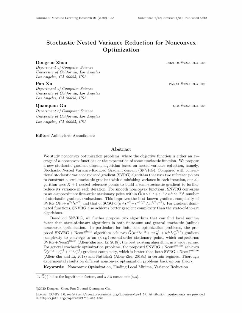
Journal of Machine Learning Research 21 (2020) 1-63 Submitted 7/18; Revised 4/20; Published 5/20
Stochastic Nested Variance Reduction for NonconvexOptimization
Dongruo Zhou [email protected] of Computer ScienceUniversity of California, Los AngelesLos Angeles, CA 90095, USA
Pan Xu [email protected] of Computer ScienceUniversity of California, Los AngelesLos Angeles, CA 90095, USA
Quanquan Gu [email protected]
Department of Computer Science
University of California, Los Angeles
Los Angeles, CA 90095, USA
Editor: Animashree Anandkumar
Abstract
We study nonconvex optimization problems, where the objective function is either an av-erage of n nonconvex functions or the expectation of some stochastic function. We proposea new stochastic gradient descent algorithm based on nested variance reduction, namely,Stochastic Nested Variance-Reduced Gradient descent (SNVRG). Compared with conven-tional stochastic variance reduced gradient (SVRG) algorithm that uses two reference pointsto construct a semi-stochastic gradient with diminishing variance in each iteration, our al-gorithm uses K + 1 nested reference points to build a semi-stochastic gradient to furtherreduce its variance in each iteration. For smooth nonconvex functions, SNVRG convergesto an ε-approximate first-order stationary point within O(n∧ ε−2 + ε−3∧n1/2ε−2)1 numberof stochastic gradient evaluations. This improves the best known gradient complexity ofSVRG O(n+n2/3ε−2) and that of SCSG O(n∧ ε−2 + ε−10/3∧n2/3ε−2). For gradient domi-nated functions, SNVRG also achieves better gradient complexity than the state-of-the-artalgorithms.
Based on SNVRG, we further propose two algorithms that can find local minimafaster than state-of-the-art algorithms in both finite-sum and general stochastic (online)nonconvex optimization. In particular, for finite-sum optimization problems, the pro-
posed SNVRG + Neon2finite algorithm achieves O(n1/2ε−2 + nε−3H + n3/4ε
−7/2H ) gradient
complexity to converge to an (ε, εH)-second-order stationary point, which outperformsSVRG+Neon2finite (Allen-Zhu and Li, 2018), the best existing algorithm, in a wide regime.For general stochastic optimization problems, the proposed SNVRG + Neon2online achievesO(ε−3 + ε−5
H + ε−2ε−3H ) gradient complexity, which is better than both SVRG + Neon2online
(Allen-Zhu and Li, 2018) and Natasha2 (Allen-Zhu, 2018a) in certain regimes. Thoroughexperimental results on different nonconvex optimization problems back up our theory.
Keywords: Nonconvex Optimization, Finding Local Minima, Variance Reduction
1. O(·) hides the logarithmic factors, and a ∧ b means min(a, b).
c©2020 Dongruo Zhou, Pan Xu and Quanquan Gu.
License: CC-BY 4.0, see https://creativecommons.org/licenses/by/4.0/. Attribution requirements are providedat http://jmlr.org/papers/v21/18-447.html.
Zhou, Xu and Gu
1. Introduction
We study the following nonconvex optimization problem: minx∈Rd F (x), where F is a non-convex smooth function. A popular example of this problem is the finite-sum optimization,where the loss function is a sum of n nonconvex component functions:
minx∈Rd
F (x) =1
n
n∑
i=1
fi(x), (1)
where each fi is defined on a different data point. The finite-sum optimization problem (1)is often regarded as the offline learning setting in the literature (Allen-Zhu and Li, 2018;Fang et al., 2018). A closely related variant of the finite-sum optimization problem in (1)is the following general stochastic optimization problem:
minx∈Rd
F (x) = Eξ∼D[F (x; ξ)], (2)
where ξ is a random variable drawn from some fixed but unknown distribution D and F (x; ξ)is a nonconvex smooth function indexed by ξ. The general stochastic optimization problemdefined in (2) encloses innumerable large-scale machine learning applications which keepgenerating oceans of data samples. Therefore, (2) is also referred to as the online learningsetting (Allen-Zhu and Li, 2018).
For either (1) or (2), finding the global minimum of such nonconvex optimizationproblems can be generally NP hard (Hillar and Lim, 2013). Therefore, instead of find-ing the global minimum, various optimization methods have been developed to find an ε-approximate first-order stationary point of (1) and (2), i.e., a point x satisfying ‖∇F (x)‖2 ≤ε, where ε > 0 is a predefined precision parameter. This vast body of literature con-sists of gradient descent (GD), stochastic gradient descent (SGD) (Robbins and Monro,1951), stochastic variance reduced gradient (SVRG) (Reddi et al., 2016a; Allen-Zhu andHazan, 2016), StochAstic Recursive grAdient algoritHm (SARAH) (Nguyen et al., 2017b)and stochastically controlled stochastic gradient (SCSG) (Lei et al., 2017). Among allthe aforementioned first-order methods, the stochastically controlled stochastic gradient(SCSG) proposed by Lei et al. (2017) achieves the lowest gradient complexity2 O(n∧ ε−2 +ε−10/3 ∧ (n2/3ε−2)), which, to the best of our knowledge, is the state-of-the-art gradientcomplexity under the smoothness (i.e., gradient Lipschitzness) and bounded stochastic gra-dient variance assumptions. The key idea behind variance reduction is that the gradientcomplexity can be saved if the algorithm use history information as reference. For instance,the representative variance reduction method SVRG is based on a semi-stochastic gradientthat is defined by two reference points. Since the the variance of this semi-stochastic gradi-ent will diminish when the iterate gets closer to the minimizer, it therefore accelerates theconvergence of stochastic gradient method. A natural and long standing question is:
Is there still room for improvement in nonconvex finite-sum optimization without makingadditional assumptions beyond smoothness and bounded stochastic gradient variance?
2. We usually use gradient complexity, the number of stochastic gradient evaluations, to measure theconvergence speed of different first-order algorithms.
2
Stochastic Nested Variance Reduction for Nonconvex Optimization
In this paper, we provide an affirmative answer to the above question, by showing thatthe dependence on n in the gradient complexity of SVRG (Reddi et al., 2016a; Allen-Zhuand Hazan, 2016) and SCSG (Lei et al., 2017) can be further reduced. We propose a novelalgorithm namely Stochastic Nested Variance-Reduced Gradient descent (SNVRG). Similarto SVRG and SCSG, our proposed algorithm works in a multi-epoch way. Nevertheless, thetechnique we developed is highly nontrivial. At the core of our algorithm is the multiplereference points-based variance reduction technique in each iteration. In detail, inspired bySVRG and SCSG, which uses two reference points to construct a semi-stochastic gradientwith diminishing variance, our algorithm uses K + 1 reference points to construct a semi-stochastic gradient, whose variance decays faster than that of the semi-stochastic gradientused in SVRG and SCSG.
Due to the nonconvexity of the objective function F (x), first-order stationary pointsare not always satisfying since they can be saddle points and even local maxima. To avoidsuch unsatisfactory stationary points, one can further pursue an (ε, εH)-approximate second-order stationary point (Nesterov and Polyak, 2006) of (1) and (2), namely a point x thatsatisfies
‖∇F (x)‖2 ≤ ε, and λmin
(∇2F (x)
)≥ −εH , (3)
where ε, εH ∈ (0, 1) are predefined precision parameters and λmin(·) denotes the minimumeigenvalue of a matrix. An (ε,
√ε)-approximate second-order stationary point is considered
as an approximate local minimum of the optimization problem (Nesterov and Polyak, 2006).In many tasks such as training a deep neural network, matrix completion and matrix sensing,one have found that local minima have a very good generalization performance (Choroman-ska et al., 2015; Dauphin et al., 2014) or all local minima are global minima (Ge et al., 2016;Bhojanapalli et al., 2016; Zhang et al., 2018). Although it has been proved that first-ordermethod such as GD can converge to local minima asymptotically (Lee et al., 2016, 2019),there is no result in the literature that establishes the convergence rate of vanilla GD/SGDalgorithms to local minima. Recently, there has emerged a large body of work (Xu et al.,2018b; Allen-Zhu and Li, 2018; Jin et al., 2018; Daneshmand et al., 2018) that only usefirst-order oracles to find the negative curvature direction. Specifically, Xu et al. (2018b)proposed a negative curvature originated from noise (NEON) algorithm that can extractthe negative curvature direction based on gradient evaluation, which saves Hessian-vectorcomputation. Later, Allen-Zhu and Li (2018) proposed a Neon2 algorithm, which furtherreduces the number of (stochastic) gradient evaluations required by NEON. Equipped withNEON and Neon2, many aforementioned algorithms such as GD, SGD, SVRG, SCSG forfinding the first-order stationary point can be turned into local minimum finding ones (Xuet al., 2018b; Allen-Zhu and Li, 2018; Yu et al., 2017, 2018).
Based on the SNVRG algorithm we proposed for finding the first-order stationary pointin nonconvex optimization, we take a step further to propose faster algorithms for find-ing the second-order stationary point. More specifically, we present two novel algorithmsthat can find local minima faster than existing algorithms (Xu et al., 2018b; Allen-Zhuand Li, 2018; Yu et al., 2018) in a wide regime for both finite-sum and stochastic opti-mization. The proposed algorithms essentially use Neon2 (Allen-Zhu and Li, 2018) to turnOne-epoch-SNVRG into a local minimum finder.
3
Zhou, Xu and Gu
1.1. Contribution
We summarize the major contributions of this paper as follows:
• We propose a stochastic nested variance reduced gradient (SNVRG) algorithm fornonconvex optimization, which reduces the dependence of the gradient complexity onn compared with SVRG and SCSG.
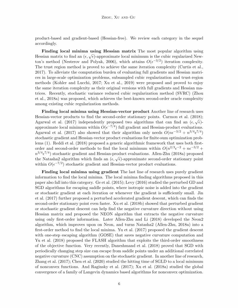
• We show that our proposed algorithm is able to find an ε-approximate stationary pointwith O(n ∧ ε−2 + ε−3 ∧ n1/2ε−2) stochastic gradient evaluations, which outperformsall existing first-order algorithms such as GD, SGD, SVRG and SCSG. A detailedcomparison is demonstrated in Figure 1.
• As a by-product, when F is a τ -gradient dominated function, a variant of our algorithmcan achieve an ε-approximate global minimizer (i.e., F (x) − miny F (y) ≤ ε) within
O(n∧ τε−1 + τ(n∧ τε−1)1/2
)stochastic gradient evaluations, which also outperforms
the state-of-the-art.
• For the finite-sum optimization setting (1), we propose an algorithm, SNVRG +Neon2finite, that can find an (ε, εH) second-order stationary point of the finite-sum
problem (1) within O(n1/2ε−2 + nε−3H + n3/4ε
−7/2H ) stochastic gradient evaluations,
which is evidently faster than the best existing algorithm SVRG + Neon2finite (Allen-
Zhu and Li, 2018) that attains O(n2/3ε−2 + nε−3H + n3/4ε
−7/2H ) gradient complexity in
a wide regime. A thorough comparison is illustrated in Figure 3.
• For the general stochastic optimization setting (2), we propose an algorithm, SNVRG+Neon2online, that can find an (ε, εH) second-order stationary point of (2) withinO(ε−3 + ε−5
H + ε−2ε−3H ) stochastic gradient evaluations, which is again faster than the
state-of-the-art algorithms such as SCSG+Neon2online (Allen-Zhu and Li, 2018) withO(ε−10/3 + ε−5
H + ε−2ε−3H ) gradient complexity, and Natasha2 (Allen-Zhu, 2018a) with
O(ε−3.25 + ε−3εH + ε−5H ) gradient complexity in certain regime. A detailed comparison
is demonstrated in Figure 4.
• We also show that our proposed algorithms can find local minima even faster whenthe objective function enjoys the third-order smoothness property. We prove thatour proposed algorithms achieve faster convergence rates to a local minimum thanthe FLASH algorithm proposed in Yu et al. (2018), which also exploits the third-order smoothness of objective functions for both finite-sum and general stochasticoptimization problems.
A short version of this paper (Zhou et al., 2018b) has been published in NeurIPS 2018,which proposes the SNVRG algorithm for finding first-order stationary points. This longerversion adds new algorithms that turn SNVRG into local minima finding algorithms.
The remainder of this paper is organized as follows: In Section 2 we review the relevantwork in the literature. We present preliminary definitions in Section 3. We then presentour SNVRG algorithm in Section 4. We present our main theoretical results for findingstationary points in Section 5. We further present two algorithms based on SNVRG to
4
Stochastic Nested Variance Reduction for Nonconvex Optimization
find local minima in Section 6. The theoretical analysis for finding local minima for second-order smooth functions is in Section 7 and that for third-order smooth functions in Section 8.Experiments on validating the advantage of SNVRG is provided in Section 9. We concludethe paper with Section 10.
Notation: Denote A = [Aij ] ∈ Rd×d as a matrix and x = (x1, ..., xd)> ∈ Rd as a vector.
‖v‖2 denotes the 2-norm of a vector v ∈ Rd. We use 〈·, ·〉 to represent the inner product.For two sequences an and bn, we denote an = O(bn) if there is a constant 0 < C < +∞such that an ≤ C bn, denote an = Ω(bn) if there is a constant 0 < C < +∞, such thatan ≥ C bn, and use O(·) to hide logarithmic factors. We also write an . bn (or an & bn)if an is less than (or larger than) bn up to a constant. We denote the product caca+1 . . . cbterm as
∏bi=a ci. In addition, if a > b, we define
∏bi=a ci = 1. In this paper, b·c represents
the floor function and log(x) represents the logarithm of x to base 2. a∧ b means min(a, b).We denote by 1E the indicator function such that 1E = 1 if the event E is true, and1E = 0 otherwise.
2. Related Work
In this section, we review and discuss the relevant work in the literature of nonconvexoptimization for solving problems (1) and (2).
Finding first-order stationary points For nonconvex optimization, it is well-knownthat Gradient Descent (GD) can converge to an ε-approximate stationary point with O(n ·ε−2) (Nesterov, 2013) number of stochastic gradient evaluations. GD needs to calculatethe full gradient at each iteration, which is a heavy load when n 1. Stochastic gradi-ent descent (SGD) (Robbins and Monro, 1951; Nesterov, 2013) and its variants (Ghadimiand Lan, 2013, 2016; Ghadimi et al., 2016) achieve O(1/ε4) gradient complexity under theassumption that the stochastic gradient has a bounded variance. Inspired by the greatsuccess of various variance reduced techniques in convex finite-sum optimization such asStochastic Average Gradient (SAG) (Roux et al., 2012), Stochastic Variance Reduced Gra-dient (SVRG) (Johnson and Zhang, 2013; Xiao and Zhang, 2014), SAGA (Defazio et al.,2014a), Stochastic Dual Coordinate Ascent (SDCA) (Shalev-Shwartz and Zhang, 2013),Finito (Defazio et al., 2014b) and Batching SVRG (Harikandeh et al., 2015), Garber andHazan (2015); Shalev-Shwartz (2016) first analyzed the convergence of SVRG under noncon-vex setting, where F is still convex but each component function fi can be nonconvex. Theanalysis for the general nonconvex function F was done by Reddi et al. (2016a); Allen-Zhuand Hazan (2016), which shows that SVRG can converge to an ε-approximate stationarypoint with O(n2/3 · ε−2) number of stochastic gradient evaluations. This result is strictlybetter than that of GD. Nguyen et al. (2017a,b) proposed StochAstic Recursive grAdientalgoritHm (SARAH) with recursive estimators for finding first-order stationary points withO(n+L2/ε4) stochastic gradient evaluations. Lei et al. (2017) proposed a new variance re-duction algorithm, i.e., the stochastically controlled stochastic gradient (SCSG) algorithm,which finds a first-order stationary point within O(minε−10/3, n2/3ε−2) stochastic gradientevaluations for finite-sum optimization in (1), and outperforms SVRG when the number ofcomponent functions n is large.
The literature of finding local minima in nonconvex optimization can be roughly di-vided into three categories according to the oracles they use: Hessian-based, Hessian-vector
5
Zhou, Xu and Gu
product-based and gradient-based (Hessian-free). We review each category in the sequelaccordingly.
Finding local minima using Hessian matrix The most popular algorithm usingHessian matrix to find an (ε,
√ε)-approximate local minimum is the cubic regularized New-
ton’s method (Nesterov and Polyak, 2006), which attains O(ε−3/2) iteration complexity.The trust region method is proved to achieve the same iteration complexity (Curtis et al.,2017). To alleviate the computation burden of evaluating full gradients and Hessian matri-ces in large-scale optimization problems, subsampled cubic regularization and trust-regionmethods (Kohler and Lucchi, 2017; Xu et al., 2019) were proposed and proved to enjoythe same iteration complexity as their original versions with full gradients and Hessian ma-trices. Recently, stochastic variance reduced cubic regularization method (SVRC) (Zhouet al., 2018a) was proposed, which achieves the best-known second-order oracle complexityamong existing cubic regularization methods.
Finding local minima using Hessian-vector product Another line of research usesHessian-vector products to find the second-order stationary points. Carmon et al. (2018);Agarwal et al. (2017) independently proposed two algorithms that can find an (ε,
√ε)-
approximate local minimum within O(ε−7/4) full gradient and Hessian-product evaluations.Agarwal et al. (2017) also showed that their algorithm only needs O(nε−3/2 + n3/4ε7/4)stochastic gradient and Hessian-vector product evaluations for finite-sum optimization prob-lems (1). Reddi et al. (2018) proposed a generic algorithmic framework that uses both first-order and second-order methods to find the local minimum within O(n2/3ε−2 + nε−3/2 +n3/4ε7/4) stochastic gradient and Hessian-product evaluations. Allen-Zhu (2018a) proposedthe Natasha2 algorithm which finds an (ε,
√ε)-approximate second-order stationary point
within O(ε−7/2) stochastic gradient and Hessian-vector product evaluations.
Finding local minima using gradient The last line of research uses purely gradientinformation to find the local minima. The local minima finding algorithms proposed in thispaper also fall into this category. Ge et al. (2015); Levy (2016) studied the perturbed GD andSGD algorithms for escaping saddle points, where isotropic noise is added into the gradientor stochastic gradient at each iteration or whenever the gradient is sufficiently small. Jinet al. (2017) further proposed a perturbed accelerated gradient descent, which can finds thesecond-order stationary point even faster. Xu et al. (2018b) showed that perturbed gradientor stochastic gradient descent can help find the negative curvature direction without usingHessian matrix and proposed the NEON algorithm that extracts the negative curvatureusing only first-order information. Later Allen-Zhu and Li (2018) developed the Neon2algorithm, which improves upon on Neon, and turns Natasha2 (Allen-Zhu, 2018a) into afirst-order method to find the local minima. Yu et al. (2017) proposed the gradient descentwith one-step escaping algorithm (GOSE) that saves negative curvature computation andYu et al. (2018) proposed the FLASH algorithm that exploits the third-order smoothnessof the objective function. Very recently, Daneshmand et al. (2018) proved that SGD withperiodically changing step size can escape from saddle points under an additional correlatednegative curvature (CNC) assumption on the stochastic gradient. In another line of research,Zhang et al. (2017); Chen et al. (2020) studied the hitting time of SGLD to a local minimumof nonconvex functions. And Raginsky et al. (2017); Xu et al. (2018a) studied the globalconvergence of a family of Langevin dynamics based algorithms for nonconvex optimization.
6
Stochastic Nested Variance Reduction for Nonconvex Optimization
SNVRGSCSGSVRG
GradientComplexity
n2
3
10/3
12
n1/2
2
n2/3
2
n2/3
2
Figure 1: Comparison of gradient complexities.
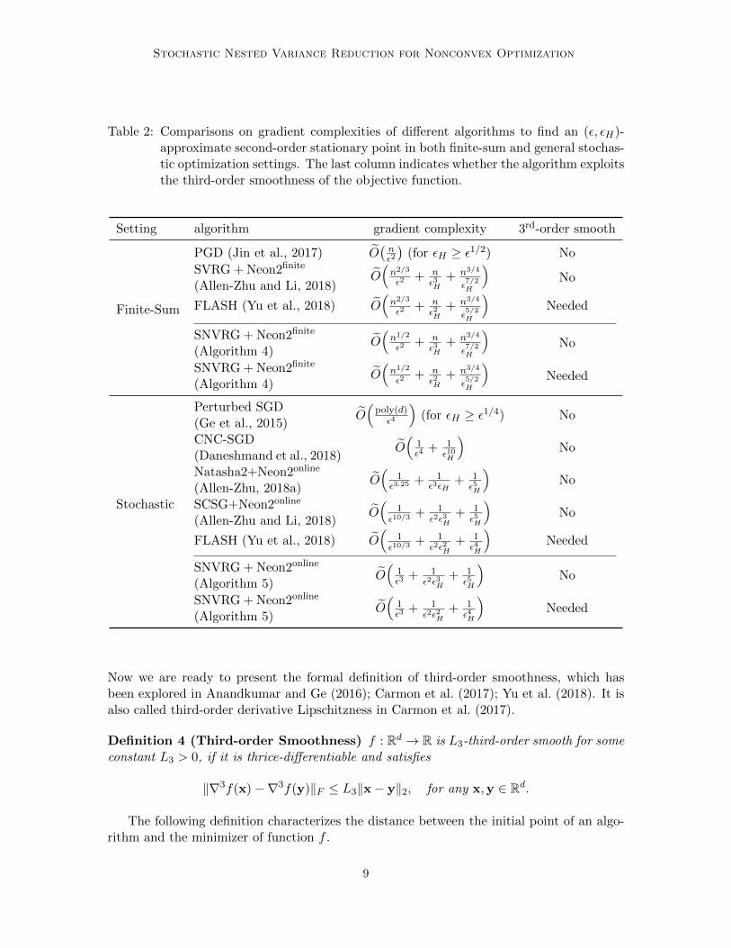
To give a thorough comparison of our proposed SNVRG algorithm with existing al-gorithms for nonconvex finite-sum optimization, we summarize the gradient complexity ofthe most relevant algorithms in Table 1 for finding first-order stationary points and inTable 2 for finding local minimum using first-order information. We also present the gra-dient complexities of first-order local minimum finding algorithms in Table 2. Accordingto Table 1, the proposed SNVRG algorithm achieves the lowest gradient complexity tofind an ε-approximate first-order stationary point for both nonconvex functions and gra-dient dominant functions. We can also see from Table 2 that our proposed algorithmsSNVRG + Neon2finite and SNVRG + Neon2online outperform all other first-order algorithmsin finding an (ε, εH)-approximate second-order stationary point for nonconvex optimizationproblems in a wide regime, for both finite-sum and general stochastic optimization.
Follow-up work after this paper After the first appearance of our SNVRG algorithmin a conference paper (Zhou et al., 2018b), there have emerged a considerable amount ofexciting work on this topic. Fang et al. (2018) concurrently proposed the Stochastic Path-Integrated Differential EstimatoR (SPIDER), which uses recursive update to define thesemi-stochastic gradient in the variance reduction algorithm. They proved that SPIDERachieves O(n1/2ε−2∧ε−3) gradient complexity for finding an ε-approximate stationary pointin nonconvex optimization. Wang et al. (2019) proposed an improved analysis for SPIDER(also called SpiderBoost) and SPIDER with momentum. Nguyen et al. (2019) proposed animproved analysis for SARAH. Tran-Dinh et al. (2019) proposed a hybrid method whichcombines SARAH (Nguyen et al., 2017a) and SGD. Note that all the aforementioned algo-rithms enjoy a similar convergence rate to SPIDER (Fang et al., 2018). Fang et al. (2018);Zhou and Gu (2019) also showed that both SPIDER and SNVRG are near optimal withrespect to the gradient complexity. In a recent work, Fang et al. (2019) proposed a tighteranalysis of the gradient complexity for SGD to escape saddle points.
3. Preliminaries
In this section, we present some definitions that will be used throughout this paper.
7
Zhou, Xu and Gu
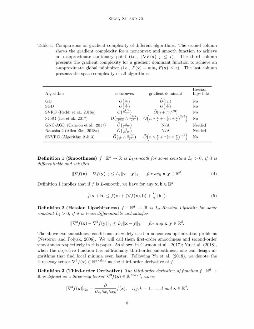
Table 1: Comparisons on gradient complexity of different algorithms. The second columnshows the gradient complexity for a nonconvex and smooth function to achievean ε-approximate stationary point (i.e., ‖∇F (x)‖2 ≤ ε). The third columnpresents the gradient complexity for a gradient dominant function to achieve anε-approximate global minimizer (i.e., F (x) − minx F (x) ≤ ε). The last columnpresents the space complexity of all algorithms.
Algorithm nonconvex gradient dominantHessianLipschitz
GD O(nε2
)O(τn) No
SGD O(
1ε4
)O(
1ε4
)No
SVRG (Reddi et al., 2016a) O(n2/3
ε2
)O(n+ τn2/3) No
SCSG (Lei et al., 2017) O(
1ε10/3
∧ n2/3
ε2
)O(n ∧ τ
ε + τ(n ∧ τ
ε
)2/3)No
GNC-AGD (Carmon et al., 2017) O(
nε1.75
)N/A Needed
Natasha 2 (Allen-Zhu, 2018a) O(
1ε3.25
)N/A Needed
SNVRG (Algorithm 2 & 3) O(
1ε3 ∧ n1/2
ε2
)O(n ∧ τ
ε + τ(n ∧ τ
ε
)1/2)No
Definition 1 (Smoothness) f : Rd → R is L1-smooth for some constant L1 > 0, if it isdifferentiable and satisfies
‖∇f(x)−∇f(y)‖2 ≤ L1‖x− y‖2, for any x,y ∈ Rd. (4)
Definition 1 implies that if f is L-smooth, we have for any x,h ∈ Rd
f(x + h) ≤ f(x) + 〈∇f(x),h〉+L
2‖h‖22. (5)
Definition 2 (Hessian Lipschitzness) f : Rd → R is L2-Hessian Lipschitz for someconstant L2 > 0, if it is twice-differentiable and satisfies
‖∇2f(x)−∇2f(y)‖2 ≤ L2‖x− y‖2, for any x,y ∈ Rd.
The above two smoothness conditions are widely used in nonconvex optimization problems(Nesterov and Polyak, 2006). We will call them first-order smoothness and second-ordersmoothness respectively in this paper. As shown in Carmon et al. (2017); Yu et al. (2018),when the objective function has additionally third-order smoothness, one can design al-gorithms that find local minima even faster. Following Yu et al. (2018), we denote thethree-way tensor ∇3f(x) ∈ Rd×d×d as the third-order derivative of f .
Definition 3 (Third-order Derivative) The third-order derivative of function f : Rd →R is defined as a three-way tensor ∇3f(x) ∈ Rd×d×d, where
[∇3f(x)]ijk =∂
∂xi∂xj∂xkf(x), i, j, k = 1, . . . , d and x ∈ Rd.
8
Stochastic Nested Variance Reduction for Nonconvex Optimization
Table 2: Comparisons on gradient complexities of different algorithms to find an (ε, εH)-approximate second-order stationary point in both finite-sum and general stochas-tic optimization settings. The last column indicates whether the algorithm exploitsthe third-order smoothness of the objective function.
Setting algorithm gradient complexity 3rd-order smooth
Finite-Sum
PGD (Jin et al., 2017) O(nε2
)(for εH ≥ ε1/2) No
SVRG + Neon2finiteO(n2/3
ε2+ n
ε3H+ n3/4
ε7/2H
)No
(Allen-Zhu and Li, 2018)
FLASH (Yu et al., 2018) O(n2/3
ε2+ n
ε2H+ n3/4
ε5/2H
)Needed
SNVRG + Neon2finiteO(n1/2
ε2+ n
ε3H+ n3/4
ε7/2H
)No
(Algorithm 4)
SNVRG + Neon2finiteO(n1/2
ε2+ n
ε2H+ n3/4
ε5/2H
)Needed
(Algorithm 4)
Stochastic
Perturbed SGDO(
poly(d)ε4
)(for εH ≥ ε1/4) No
(Ge et al., 2015)CNC-SGD
O(
1ε4
+ 1ε10H
)No
(Daneshmand et al., 2018)Natasha2+Neon2online
(Allen-Zhu, 2018a)O(
1ε3.25
+ 1ε3εH
+ 1ε5H
)No
SCSG+Neon2online
O(
1ε10/3
+ 1ε2ε3H
+ 1ε5H
)No
(Allen-Zhu and Li, 2018)
FLASH (Yu et al., 2018) O(
1ε10/3
+ 1ε2ε2H
+ 1ε4H
)Needed
SNVRG + Neon2online
O(
1ε3
+ 1ε2ε3H
+ 1ε5H
)No
(Algorithm 5)
SNVRG + Neon2online
O(
1ε3
+ 1ε2ε2H
+ 1ε4H
)Needed
(Algorithm 5)
Now we are ready to present the formal definition of third-order smoothness, which hasbeen explored in Anandkumar and Ge (2016); Carmon et al. (2017); Yu et al. (2018). It isalso called third-order derivative Lipschitzness in Carmon et al. (2017).
Definition 4 (Third-order Smoothness) f : Rd → R is L3-third-order smooth for someconstant L3 > 0, if it is thrice-differentiable and satisfies
‖∇3f(x)−∇3f(y)‖F ≤ L3‖x− y‖2, for any x,y ∈ Rd.
The following definition characterizes the distance between the initial point of an algo-rithm and the minimizer of function f .
9
Zhou, Xu and Gu
Definition 5 (Optimal Gap) The optimal gap of f at point x0 is denoted by ∆f and
f(x0)− minx∈Rd
f(x) ≤ ∆f .
W.L.O.G., we assume ∆f < +∞.
Definition 6 f : Rd → R is λ-strongly convex for some constant λ > 0, if it satisfies
f(x + h) ≥ f(x) + 〈∇f(x),h〉+λ
2‖h‖22, for any x,y ∈ Rd. (6)
While the above definitions are based on a general function f , the following two defini-tions rely on the finite-sum structure of F defined in (1).
Definition 7 A function F with finite-sum structure in (1) is said to have stochastic gra-dients with bounded variance σ2, if for any x ∈ Rd, we have
Ei‖∇fi(x)−∇F (x)‖22 ≤ σ2, (7)
where i a random index uniformly chosen from [n] and Ei denotes the expectation over suchi.
σ2 is called the upper bound on the variance of stochastic gradients (Lei et al., 2017).
Definition 8 A function F with finite-sum structure in (1) is said to have averaged L-Lipschitz gradient, if for any x,y ∈ Rd, we have
Ei‖∇fi(x)−∇fi(y)‖22 ≤ L2‖x− y‖22, (8)
where i is a random index uniformly chosen from [n] and Ei denotes the expectation overthe choice.
It should be noted that the smoothness condition of each fi in Definition 1 will directlyimply the averaged L-Lipschitz gradient for F .
We also consider a class of functions namely gradient dominated functions (Polyak,1963), which is formally defined as follows:
Definition 9 We say function f is τ -gradient dominated if for any x ∈ Rd, we have
f(x)− f(x∗) ≤ τ · ‖∇f(x)‖22, (9)
where x∗ ∈ Rd is the global minimum of f .
Note that gradient dominated condition is also known as the Polyak-Lojasiewicz (P-L)condition (Polyak, 1963), and is not necessarily convex. It is weaker than strong convexityas well as other popular conditions that appear in the optimization literature (Karimi et al.,2016).
Inspired by the SCSG algorithm (Lei et al., 2017), we will use the property of geometricdistribution in our algorithm design. The definition of geometric random variable is asfollows.
10
Stochastic Nested Variance Reduction for Nonconvex Optimization
Definition 10 (Geometric Distribution) A random variable X follows a geometric dis-tribution with parameter p, denoted as Geom(p), if it holds that
P(X = k) = p(1− p)k, ∀k = 0, 1, . . . .
Definition 11 (Sub-Gaussian Stochastic Gradient) We say a function F has σ2-sub-Gaussian stochastic gradient ∇F (x; ξ) for any x ∈ Rd and random variable ξ ∼ D, if itsatisfies
E[
exp
(‖∇F (x; ξ)−∇f(x)‖22σ2
)]≤ exp(1).
Note that Definition 11 implies E[‖∇F (x; ξ) − ∇f(x)‖22] ≤ 2σ2 (Vershynin, 2010). In thefinite-sum optimization setting (1), we call ∇fi(x) a stochastic gradient of function F fora randomly chosen index i ∈ [n], and we say F has σ2-sub-Gaussian stochastic gradient ifE[‖∇fi(x)−∇F (x)‖22] ≤ 2σ2.
4. Stochastic Nested Variance-Reduced Gradient Descent
In this section, we present our nested stochastic variance reduction algorithm, namely,SNVRG for finding first-order stationary points in nonconvex optimization.
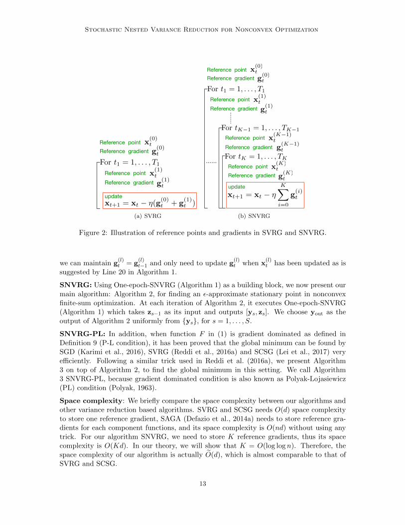
One-epoch-SNVRG: We first present the key component of our main algorithm, One-epoch-SNVRG, which is displayed in Algorithm 1. The most innovative part of Algorithm 1attributes to theK+1 reference points andK+1 reference gradients. Note that whenK = 1,Algorithm 1 reduces to one epoch of SVRG algorithm (Johnson and Zhang, 2013; Reddiet al., 2016a; Allen-Zhu and Hazan, 2016). To better understand our One-epoch-SNVRGalgorithm, it would be helpful to revisit the original SVRG which is a special case of ouralgorithm. For the finite-sum optimization problem in (1), the original SVRG takes thefollowing updating formula
xt+1 = xt − ηvt = xt − η(∇F (x) +∇fit(xt)−∇fit(x)
),
where η > 0 is the step size, it is a random index uniformly chosen from [n] and x is asnapshot for xt after every T1 iterations. There are two reference points in the update
formula at xt: x(0)t = x and x
(1)t = xt. Note that x is updated every T1 iterations,
namely, x is set to be xt only when (t mod T1) = 0. Moreover, in the semi-stochastic
gradient vt, there are also two reference gradients and we denote them by g(0)t = ∇F (x)
and g(1)t = ∇fit(xt)−∇fit(x) = ∇fit(x(1)
t )−∇fit(x(0)t ).
Back to our One-epoch-SNVRG, we can define similar reference points and referencegradients as that in the special case of SVRG. Specifically, for t = 0, . . . ,
∏Kl=1 Tl − 1, each
point xt has K + 1 reference points x(l)t , l = 0, . . . ,K, which is set to be x
(l)t = xtl with
index tl defined as
tl =
⌊t
∏Kk=l+1 Tk
⌋·
K∏
k=l+1
Tk. (10)
11
Zhou, Xu and Gu
Algorithm 1 One-epoch-SNVRG(x0, F,K,M, Tl, Bl, B0)
1: Input: initial point x(l)−1 ← x0, l ∈ [K]; function F ; loop number K; step size parameter
M ; loop parameters Tl; batch parameters Bl, base batch size B0.2: Option I T =
∏Kl=1 Tl
3: Option II T ∼ Geom(1/(1 +∏Kl=1 Tl))
4: for t = 0, . . . , T − 1 do5: r = minj : 0 = (t mod
∏Kl=j+1 Tl), 0 ≤ j ≤ K
6: x(l)t ← Update reference points(x(l)
t−1,xt, r), 0 ≤ l ≤ K.
7: g(l)t ← Update reference gradients(g(l)
t−1, x(l)t , r), 0 ≤ l ≤ K.
8: vt ←∑K
l=0 g(l)t
9: xt+1 ← xt − 1/(10M) · vt10: end for11: xout ← uniformly random choice from xt, where 0 ≤ t <∏K
l=1 Tl12: Output: [xout,xT ]
13: Function: Update reference points(x(l)old,x, r)
14: x(l)new ← x
(l)old, 0 ≤ l ≤ r − 1; x
(l)new ← x, r ≤ l ≤ K
15: return x(l)new
16: Function: Update reference gradients(g(l)old, x
(l)new, r)
17: if r > 0 then18: g
(l)new ← g
(l)old, 0 ≤ l < r; g
(l)new ← 0, r + 1 ≤ l ≤ K
19: Uniformly generate index set I ⊂ [n] without replacement, |I| = Br
20: g(r)new ← 1/Br
∑i∈I[∇fi(x(r)
new)−∇fi(x(r−1)new )
]
21: else22: Uniformly generate index set I ⊂ [n] without replacement, |I| = B0
23: g(0)new ← 1/B0
∑i∈I ∇fi(x
(0)new); g
(l)new ← 0, 1 ≤ l ≤ K
24: end if25: return g(l)
new.
Specially, note that we have x(0)t = x0 and x
(K)t = xt for all t = 0, . . . ,
∏Kl=1 Tl−1. Similarly,
xt also has K + 1 reference gradients g(l)t , which can be defined based on the reference
points x(l)t :
g(0)t =
1
B
∑
i∈I∇fi(x0), g
(l)t =
1
Bl
∑
i∈Il
[∇fi(x(l)
t )−∇fi(x(l−1)t )
], l = 1, . . . ,K, (11)
where I, Il are random index sets with |I| = B, |Il| = Bl and are uniformly generated from[n] without replacement. Based on the reference points and reference gradients, we then
update xt+1 = xt − 1/(10M) · vt, where vt =∑K
l=0 g(l)t and M is the step size parameter.
The illustration of reference points and gradients of SNVRG is displayed in Figure 2(b).
We remark that it would be a huge waste for us to re-evaluate g(l)t at each iteration.
Fortunately, due to the fact that each reference point is only updated after a long period,
12
Stochastic Nested Variance Reduction for Nonconvex Optimization
For t1 = 1, . . . , T1
x(1)tReference point
x(0)tReference pointg
(0)tReference gradient
g(1)t
Reference gradient
updatext+1 = xt (g
(0)t + g
(1)t )
(a) SVRG
For t1 = 1, . . . , T1
For tK = 1, . . . , TK
For tK1 = 1, . . . , TK1
x(1)tReference point
x(K1)tReference point
x(K)tReference point
x(0)tReference point
g(K1)tReference gradient
g(K)t
Reference gradient
g(0)tReference gradient
g(1)t
Reference gradient
xt+1 = xt
KX
i=0
g(i)t
update
……
......
(b) SNVRG
Figure 2: Illustration of reference points and gradients in SVRG and SNVRG.
we can maintain g(l)t = g
(l)t−1 and only need to update g
(l)t when x
(l)t has been updated as is
suggested by Line 20 in Algorithm 1.
SNVRG: Using One-epoch-SNVRG (Algorithm 1) as a building block, we now present ourmain algorithm: Algorithm 2, for finding an ε-approximate stationary point in nonconvexfinite-sum optimization. At each iteration of Algorithm 2, it executes One-epoch-SNVRG(Algorithm 1) which takes zs−1 as its input and outputs [ys, zs]. We choose yout as theoutput of Algorithm 2 uniformly from ys, for s = 1, . . . , S.
SNVRG-PL: In addition, when function F in (1) is gradient dominated as defined inDefinition 9 (P-L condition), it has been proved that the global minimum can be found bySGD (Karimi et al., 2016), SVRG (Reddi et al., 2016a) and SCSG (Lei et al., 2017) veryefficiently. Following a similar trick used in Reddi et al. (2016a), we present Algorithm3 on top of Algorithm 2, to find the global minimum in this setting. We call Algorithm3 SNVRG-PL, because gradient dominated condition is also known as Polyak-Lojasiewicz(PL) condition (Polyak, 1963).
Space complexity: We briefly compare the space complexity between our algorithms andother variance reduction based algorithms. SVRG and SCSG needs O(d) space complexityto store one reference gradient, SAGA (Defazio et al., 2014a) needs to store reference gra-dients for each component functions, and its space complexity is O(nd) without using anytrick. For our algorithm SNVRG, we need to store K reference gradients, thus its spacecomplexity is O(Kd). In our theory, we will show that K = O(log log n). Therefore, thespace complexity of our algorithm is actually O(d), which is almost comparable to that ofSVRG and SCSG.
13
Zhou, Xu and Gu
Algorithm 2 SNVRG(z0, F,K,M, Tl, Bl, B0, S)
1: Input: initial point z0; function F ; loop numbers K,S; step size parameter M ; loopparameters Tl; batch parameters Bl; base batch size B0.
2: for s = 1, . . . , S do3: [ys, zs] = One-epoch-SNVRG(zs−1, F,K,M, Tl, Bl, B0) . Algorithm 1 with
Option I4: end for5: Output: Uniformly choose yout from ys, 1 ≤ s ≤ S.
Algorithm 3 SNVRG-PL(z0, F,K,M, Tl, Bl, B0, S, U)
1: Input: initial point z0; function F ; loop number K,S; step size parameter M ; loopparameters Tl; batch parameters Bl; base batch size B0; outer loop number U .
2: for u = 1, . . . , U do3: zu = SNVRG(zu−1, F,K,M, Tl, Bl, B0, S) . Algorithm 24: end for5: Output: zout = zU .
5. Theoretical Analysis of SNVRG
In this section, we provide the convergence analysis of SNVRG. We will assume that F hasthe finite-sum structure in (1) throughout this section.
5.1. Convergence of SNVRG
The following theorem shows the gradient complexity for Algorithm 2 to find an ε-approximatestationary point with a constant base batch size B0.
Theorem 12 Suppose that F has averaged L-Lipschitz gradient and stochastic gradientswith bounded variance σ2. In Algorithm 2, let B0 = n ∧ (2Cσ2/ε2) and suppose B0 > 4,
S = 1 ∨ (2CL∆F /(B1/20 ε2)) and C = 6000. The rest parameters (K,M, Bl, Tl) are
chosen as follows:
K = blog logB0c,M = 6L1,
T1 =⌊B2−K
0
⌋, Tl =
⌊B2l−K−2
0
⌋, for 2 ≤ l ≤ K,
Bl = 6K−l+1
( K∏
s=l
Ts
)2
, for 1 ≤ l ≤ K. (12)
Then the output yout of Algorithm 2 satisfies E[‖∇F (yout)‖22] ≤ ε2 with less than
O
(log3
(σ2
ε2∧ n)[
σ2
ε2∧ n+
L∆F
ε2
[σ2
ε2∧ n]1/2])
(13)
stochastic gradient computations, where ∆F = F (z0)− F ∗.
14
Stochastic Nested Variance Reduction for Nonconvex Optimization
Remark 13 If we treat σ2, L and ∆F as constants, and assume ε 1, then (13) can besimplified to O(ε−3 ∧ n1/2ε−2). This gradient complexity is strictly better than O(ε−10/3 ∧n2/3ε−2), which is achieved by SCSG (Lei et al., 2017). Specifically, when n . 1/ε2, ourproposed SNVRG is faster than SCSG by a factor of n1/6; when n & 1/ε2, SNVRG is fasterthan SCSG by a factor of ε−1/3. Moreover, SNVRG also outperforms Natasha 2 (Allen-Zhu, 2018a) which attains O(ε−3.25) gradient complexity and needs the additional HessianLipschitz condition.
5.2. Convergence of SNVRG-PL
We now consider the case when F is a τ -gradient dominated function. In general, weare able to find an ε-approximate global minimizer of F instead of only an ε-approximatestationary point. Algorithm 3 uses Algorithm 2 as a component.
Theorem 14 Suppose that F has averaged L-Lipschitz gradient and stochastic gradientswith bounded variance σ2, F is a τ -gradient dominated function. In Algorithm 3, let thebase batch size B0 = n∧ (4C1τσ
2/ε) and suppose B0 > 4, the number of epochs for SNVRG
S = 1 ∨ (2C1τL/B1/20 ) and the number of epochs U = log(2∆F /ε). The rest parameters
(K,M, Bl, Tl) are chosen as the same in Lemma 28. Then the output zout of Algorithm3 satisfies E
[F (zout)− F ∗
]≤ ε within
O
(log3
(n ∧ τσ
2
ε
)log
∆F
ε
[n ∧ τσ
2
ε+ τL
[n ∧ τσ
2
ε
]1/2])(14)
stochastic gradient computations, where ∆F = F (z0)− F ∗
Remark 15 If we treat σ2, L and ∆F as constants, then the gradient complexity in (14)turns into O(n ∧ τε−1 + τ(n ∧ τε−1)1/2). Compared with nonconvex SVRG (Reddi et al.,2016b) which achieves O(n+ τn2/3) gradient complexity, our SNVRG-PL is strictly betterthan SVRG in terms of the first summand and is faster than SVRG at least by a factor ofn1/6 in terms of the second summand. Compared with a more general variant of SVRG,namely, the SCSG algorithm (Lei et al., 2017), which attains O
(n∧ τε−1 + τ(n∧ τε−1)2/3
)
gradient complexity, SNVRG-PL also outperforms it by a factor of (n ∧ τε−1)1/6.
If we further assume that F is λ-strongly convex, then it is easy to verify that F is also1/(2λ)-gradient dominated. As a direct consequence, we have the following corollary:
Corollary 16 Under the same conditions and parameter choices as Theorem 14. If we ad-ditionally assume that F is λ-strongly convex, then Algorithm 3 will outputs an ε-approximateglobal minimizer within
O
(n ∧ λσ
2
ε+ κ ·
[n ∧ λσ
2
ε
]1/2)(15)
stochastic gradient computations, where κ = L/λ is the condition number of F .
Remark 17 Corollary 16 suggests that when we regard λ and σ2 as constants and set ε 1,Algorithm 3 is able to find an ε-approximate global minimizer within O(n+n1/2κ) stochastic
15
Zhou, Xu and Gu
gradient computations, which matches SVRG1ep in Katyusha X (Allen-Zhu, 2018b). Usingcatalyst techniques (Lin et al., 2015) or Katyusha momentum (Allen-Zhu, 2017), it canbe further accelerated to O(n + n3/4√κ), which matches the best-known convergence rate(Shalev-Shwartz, 2016; Allen-Zhu, 2018b).
6. Stochastic Nested Variance Reduction for Finding Local Minima
In this section, we present our algorithms that are built upon One-epoch-SNVRG (Al-gorithm 1) and Neon2 (Allen-Zhu and Li, 2018) to find a local minimum in nonconvexoptimization faster than existing methods. It is worth noting that to find local minima, weemploy a different choice of the number of iteration T which is chosen to be a random vari-able following a geometric distribution (Algorithm 1 with Option II) rather than fixed. Wewill show in the next section that these differences are essential in the theoretical analysisof finding local minima.
6.1. SNVRG + Neon2: Finding Local Minima
We propose two different algorithms for solving the finite-sum optimization problem in (1)and the general stochastic optimization problem in (2) respectively.
To solve the finite-sum optimization problem (1), we propose the SNVRG + Neon2finite
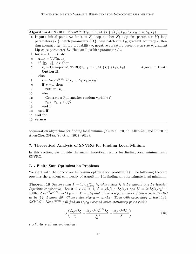
algorithm to find the local minimum, which is displayed in Algorithm 4. At each iterationof 4, it first determines whether the current point is a first-order stationary point (Line 4)or not. If not, it will run Algorithm 1 (One-epoch-SNVRG) in order to find a first-orderstationary point. Once obtaining a first-order stationary point, it will call Neon2finite tofind the negative curvature direction to escape any potential non-degenerate saddle point.According to Xu et al. (2018b); Allen-Zhu and Li (2018), Neon-type algorithms can outputsuch a direction with probability 1− δ for some failure probability δ ∈ (0, 1). If Neon2finite
does not find such a direction, it will output v =⊥ and Algorithm 4 terminates and outputszu−1 (Line 9) since it has already reached a second-order stationary point according to(3). If Neon2finite finds a negative curvature direction v 6=⊥, Algorithm 4 will perform onestep of negative curvature descent in the direction of v or −v (Line 12) to escape the non-degenerate saddle point. The direction can also be chosen in the same way as in Carmonet al. (2017) via comparing the function values at the two resulting points. Here to reducethe computational complexity, we follow Xu et al. (2018b) and generate a Rademacherrandom variable to decide the direction, which leads to the same result in expectation.
To solve the general stochastic optimization problem in (2), we propose the SNVRG +Neon2online algorithm to find the local minimum, which is displayed in Algorithm 5. Itis almost the same as Algorithm 4 used in the finite-sum nonconvex optimization settingexcept that it uses a subsampled gradient to determine whether we have obtained a first-order stationary point (Line 5 in Algorithm 5) and it uses Neon2online (Line 8) to findthe negative curvature direction to escape the potential saddle points. Algorithm 5 willterminate and output the current iterate if no negative curvature direction is found (Line 10).
Note that both Algorithms 4 and 5 are only based on the gradient information of theobjective function and are therefore first-order optimization algorithms. As we will showin the next two sections, our proposed algorithms push the frontier of first-order stochastic
16
Stochastic Nested Variance Reduction for Nonconvex Optimization
Algorithm 4 SNVRG + Neon2finite(z0, F,K,M, Tl, Bl, B0, U, ε, εH , δ, η, L1, L2)
1: Input: initial point z0; function F ; loop number K; step size parameter M ; loopparameters Tl; batch parameters Bl; base batch size B0; gradient accuracy ε; Hes-sian accuracy εH ; failure probability δ; negative curvature descent step size η; gradientLipschitz parameter L1; Hessian Lipschitz parameter L2.
2: for u = 1, . . . , U do3: gu−1 = ∇F (zu−1)4: if ‖gu−1‖2 ≥ ε then5: zu = One-epoch-SNVRG(zu−1,F,K,M, Tl, Bl, B0) . Algorithm 1 with
Option II6: else7: v = Neon2finite(F, zu−1, L1, L2, δ, εH)8: if v =⊥ then9: return zu−1
10: else11: Generate a Rademacher random variable ζ12: zu ← zu−1 + ζηv13: end if14: end if15: end for16: return
optimization algorithms for finding local minima (Xu et al., 2018b; Allen-Zhu and Li, 2018;Allen-Zhu, 2018a; Yu et al., 2017, 2018).
7. Theoretical Analysis of SNVRG for Finding Local Minima
In this section, we provide the main theoretical results for finding local minima usingSNVRG.
7.1. Finite-Sum Optimization Problems
We start with the nonconvex finite-sum optimization problem (1). The following theoremprovides the gradient complexity of Algorithm 4 in finding an approximate local minimum.
Theorem 18 Suppose that F = 1/n∑n
i=1 fi, where each fi is L1-smooth and L2-HessianLipschitz continuous. Let 0 < ε, εH < 1, δ = ε3H/(144L2
2∆F ) and U = 24L22∆F ε
−3H +
1800L1∆F ε−2n−1/2. Set B0 = n,M = 6L1 and all the rest parameters of One-epoch-SNVRG
as in (12) Lemma 29. Choose step size η = εH/L2. Then with probability at least 1/4,SNVRG + Neon2finite will find an (ε, εH)-second-order stationary point within
O
(∆FnL
22
ε3H+
∆Fn3/4L
1/21 L2
2
ε7/2H
+∆Fn
1/2L1
ε2
)(16)
stochastic gradient evaluations.
17
Zhou, Xu and Gu
Algorithm 5 SNVRG + Neon2online(z0, F,K,M, Tl, Bl, U, ε, εH , δ, η, L1, L2)
1: Input: initial point z0; function F ; loop number K; step size parameter M ; loopparameters Tl; batch parameters Bl; base batch size B0; gradient accuracy ε; Hes-sian accuracy εH ; failure probability δ; negative curvature descent step size η; gradientLipschitz parameter L1; Hessian Lipschitz parameter L2.
2: for u = 1, . . . , U do3: Uniformly generate index set I ⊂ [n] without replacement, |I| = B0
4: gu−1 = 1/B0∑
i∈I ∇fi(zu−1)5: if ‖gu−1‖2 ≥ ε/2 then6: zu = One-epoch-SNVRG(zu−1,F,K,M, Tl, Bl, B0) . Algorithm 1 with
Option II7: else8: v = Neon2online(F, zu−1, L1, L2, δ, εH)9: if v =⊥ then
10: return zu−1
11: else12: Generate a Rademacher random variable ζ13: zu ← zu−1 + ζηv14: end if15: end if16: end for17: return
Remark 19 Note that the gradient complexity in Theorem 18 holds with constant proba-bility 1/4. In practice, we can repeatedly run Algorithm 4 for log(1/p) times to achieve aresult that holds with probability at least 1−p for any p ∈ (0, 1). Similar boosting techniqueshave also been used in Yu et al. (2017); Allen-Zhu and Li (2018); Yu et al. (2018).
Remark 20 For finite-sum nonconvex optimization, Theorem 18 suggests that the gradient
complexity of Algorithm 4 (SNVRG + Neon2finite) is O(n1/2ε−2 + nε−3H + n3/4ε
−7/2H ). In
contrast, the gradient complexity of other state-of-the-art local minimum finding algorithms
(SVRG + Neon2finite) (Allen-Zhu and Li, 2018) is O(n2/3ε−2 + nε−3H + n3/4ε
−7/2H ). Our
algorithm is strictly better than that of Allen-Zhu and Li (2018) in terms of the first termin the big O notation.
If we choose εH =√ε, the gradient complexity of our algorithm to find an (ε,
√ε)-
approximate local minimum turns out to be O(n1/2ε−2 + nε−3/2 + n3/4ε−7/4) and that ofSVRG + Neon2finite is O(n2/3ε−2 + nε−3/2 + n3/4ε−7/4). We compare these two algorithmsin Figure 3 when εH =
√ε and make the following comments:
• When n & ε−3/2, the gradient complexities of both algorithms are in the same orderof O(nε−3/2).
• When ε−1 . n . ε−3/2, SNVRG + Neon2finite enjoys O(nε−3/2) gradient complexity,which is strictly better than that of SVRG + Neon2finite, i.e., O(n2/3ε−2).
18
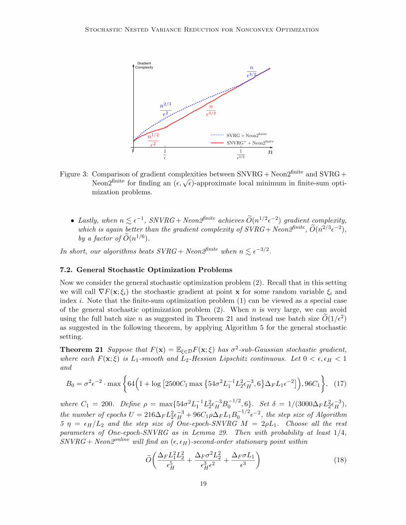
Stochastic Nested Variance Reduction for Nonconvex Optimization
1
1
3/2n
GradientComplexity
1
n1/2
2
n2/3
2n
3/2
n
3/2
SNVRG+ + Neon2finite
SVRG + Neon2finite
Figure 3: Comparison of gradient complexities between SNVRG + Neon2finite and SVRG +Neon2finite for finding an (ε,
√ε)-approximate local minimum in finite-sum opti-
mization problems.
• Lastly, when n . ε−1, SNVRG + Neon2finite achieves O(n1/2ε−2) gradient complexity,which is again better than the gradient complexity of SVRG + Neon2finite, O(n2/3ε−2),by a factor of O(n1/6).
In short, our algorithms beats SVRG + Neon2finite when n . ε−3/2.
7.2. General Stochastic Optimization Problems
Now we consider the general stochastic optimization problem (2). Recall that in this settingwe will call ∇F (x; ξi) the stochastic gradient at point x for some random variable ξi andindex i. Note that the finite-sum optimization problem (1) can be viewed as a special caseof the general stochastic optimization problem (2). When n is very large, we can avoidusing the full batch size n as suggested in Theorem 21 and instead use batch size O(1/ε2)as suggested in the following theorem, by applying Algorithm 5 for the general stochasticsetting.
Theorem 21 Suppose that F (x) = Eξ∈DF (x; ξ) has σ2-sub-Gaussian stochastic gradient,where each F (x; ξ) is L1-smooth and L2-Hessian Lipschitz continuous. Let 0 < ε, εH < 1and
B0 = σ2ε−2 ·max
64(
1 + log[2500C1 max
54σ2L−1
1 L22ε−3H , 6
∆FL1ε
−2]), 96C1
, (17)
where C1 = 200. Define ρ = max54σ2L−11 L2
2ε−3H B
−1/20 , 6. Set δ = 1/(3000∆FL
22ε−3H ),
the number of epochs U = 216∆FL22ε−3H + 96C1ρ∆FL1B
−1/20 ε−2, the step size of Algorithm
5 η = εH/L2 and the step size of One-epoch-SNVRG M = 2ρL1. Choose all the restparameters of One-epoch-SNVRG as in Lemma 29. Then with probability at least 1/4,SNVRG + Neon2online will find an (ε, εH)-second-order stationary point within
O
(∆FL
21L
22
ε5H+
∆Fσ2L2
2
ε3Hε2
+∆FσL1
ε3
)(18)
19
Zhou, Xu and Gu
SNVRG+ + Neon2online
SCSG + Neon2online
Natasha2 + Neon2online
1
3H
1
23H
1
23H
1
5H
1
5H
1
5H
GradientComplexity
H3/4 1/23.5
5
(a) εH <√ε
SNVRG+ + Neon2online
SCSG + Neon2online
Natasha2 + Neon2online
1
23H
1
23H
1
3H
GradientComplexity
3.5
10/3
3.25
3
1/2 4/9 1/3 1/4 H
(b) εH ≥√ε
Figure 4: Comparison of gradient complexities among SNVRG + Neon2online, SCSG +Neon2online and Natasha2+Neon2online for finding an (ε, εH)-approximate second-order stationary point: (a) the comparison when εH <
√ε, and (b) the comparison
when εH ≥√ε.
stochastic gradient evaluations.
The gradient complexity in Theorem 21 again holds with constant probability 1/4 and wecan boost it to a high probability using the same trick as we discussed in Remark 19.
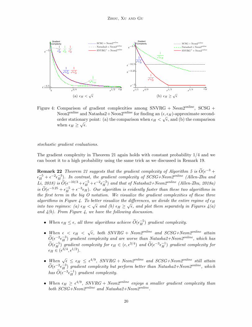
Remark 22 Theorem 21 suggests that the gradient complexity of Algorithm 5 is O(ε−3 +ε−5H + ε−2ε−3
H ). In contrast, the gradient complexity of SCSG+Neon2online (Allen-Zhu and
Li, 2018) is O(ε−10/3 + ε−5H + ε−2ε−3
H ) and that of Natasha2+Neon2online (Allen-Zhu, 2018a)
is O(ε−3.25 + ε−5H + ε−3εH). Our algorithm is evidently faster than these two algorithms in
the first term in the big O notation. We visualize the gradient complexities of these threealgorithms in Figure 4. To better visualize the differences, we divide the entire regime of εHinto two regimes: (a) εH <
√ε and (b) εH ≥
√ε, and plot them separately in Figures 4(a)
and 4(b). From Figure 4, we have the following discussion.
• When εH ≤ ε, all three algorithms achieve O(ε−5H ) gradient complexity.
• When ε < εH <√ε, both SNVRG + Neon2online and SCSG+Neon2online attain
O(ε−2ε−3H ) gradient complexity and are worse than Natasha2+Neon2online, which has
O(ε−5H ) gradient complexity for εH ∈ (ε, ε3/4) and O(ε−3ε−1
H ) gradient complexity forεH ∈ (ε3/4, ε1/2).
• When√ε ≤ εH ≤ ε4/9, SNVRG + Neon2online and SCSG+Neon2online still attain
O(ε−2ε−3H ) gradient complexity but perform better than Natasha2+Neon2online, which
has O(ε−3ε−1H ) gradient complexity.
• When εH ≥ ε4/9, SNVRG + Neon2online enjoys a smaller gradient complexity thanboth SCSG+Neon2online and Natasha2+Neon2online.
20
Stochastic Nested Variance Reduction for Nonconvex Optimization
In particular, when εH = ε1/3, the gradient complexity of our algorithm SNVRG+Neon2online
is smaller than that of SCSG+Neon2online and Natasha2+Neon2online by a factor of O(ε1/3).And when εH ≥ ε1/4, SNVRG+Neon2online is faster than Natasha2+Neon2online by a factorof O(ε1/4).
8. Theoretical Analysis of SNVRG for Finding Local Minima withThird-Order Smoothness
As we mentioned before, it has been shown that the third-order smoothness of the objectivefunction F can help accelerate the convergence of nonconvex optimization (Carmon et al.,2017; Yu et al., 2018). For the intuition of the acceleration by third-order smoothness, werefer readers to the detailed exhibition and discussion in Yu et al. (2018). In this section,we will show that our local minimum finding algorithms (Algorithms 4 and 5) can find localminima faster provided this additional condition.
8.1. Finite-Sum Optimization Problems
We first consider the finite-sum optimization problem in (1). The following theorem spellsout the gradient complexity of Algorithm 4 under additional third-order smoothness.
Theorem 23 Suppose that F = 1/n∑n
i=1 fi, where each fi is L1-smooth, L2-Hessian Lip-schitz continuous and F is L3-third-order smooth. Let 0 < ε, εH < 1, δ = ε2H/(72L3∆F ) andU = 12L3∆F ε
−2H + 1800CL1∆F ε
−2n−1/2. Set B0 = n,M = 6L1 and all the rest parameters
of One-epoch-SNVRG as in Lemma 29. Choose the step size as η =√
3εH/L3. Then withprobability at least 1/4, SNVRG + Neon2finite will find an (ε, εH)-second-order stationarypoint within
O
(∆FnL3
ε2H+
∆Fn3/4L
1/21 L3
ε5/2H
+∆Fn
1/2L1
ε2
)(19)
stochastic gradient evaluations.
Similar to previous discussions, we can repeatedly run Algorithm 4 for log(1/p) times toboost its confidence to 1− p for any p ∈ (0, 1).
Remark 24 Compared with step size η = εH/L2 used in the negative curvature descent step(Line 12) of Algorithm 4 in Theorem 18 without third-order smoothness, the step size inTheorem 23 is chosen to be η =
√εH/L3 where L3 is the third-order smoothness parameter.
Note that when εH 1, the step size we choose under third-order smoothness assumptionis much bigger than that under only second-order smoothness assumption. As is pointed outby Yu et al. (2018), the key advantage of third-order smoothness condition is that it enablesus to choose a larger step size and therefore achieve much more function value decrease inthe negative curvature descent step (Line 12 of Algorithm 4).
Remark 25 Theorem 23 suggests that the gradient complexity of SNVRG + Neon2finite un-
der third-order smoothness is O(n1/2ε−2 +nε−2H +n3/4ε
−5/2H ). In stark contrast, the gradient
complexity of the state-of-the-art finite-sum local minimum finding algorithm with third-
order smoothness assumption (FLASH) (Yu et al., 2018) is O(n2/3ε−2 +nε−2H +n3/4ε
−5/2H ).
21
Zhou, Xu and Gu
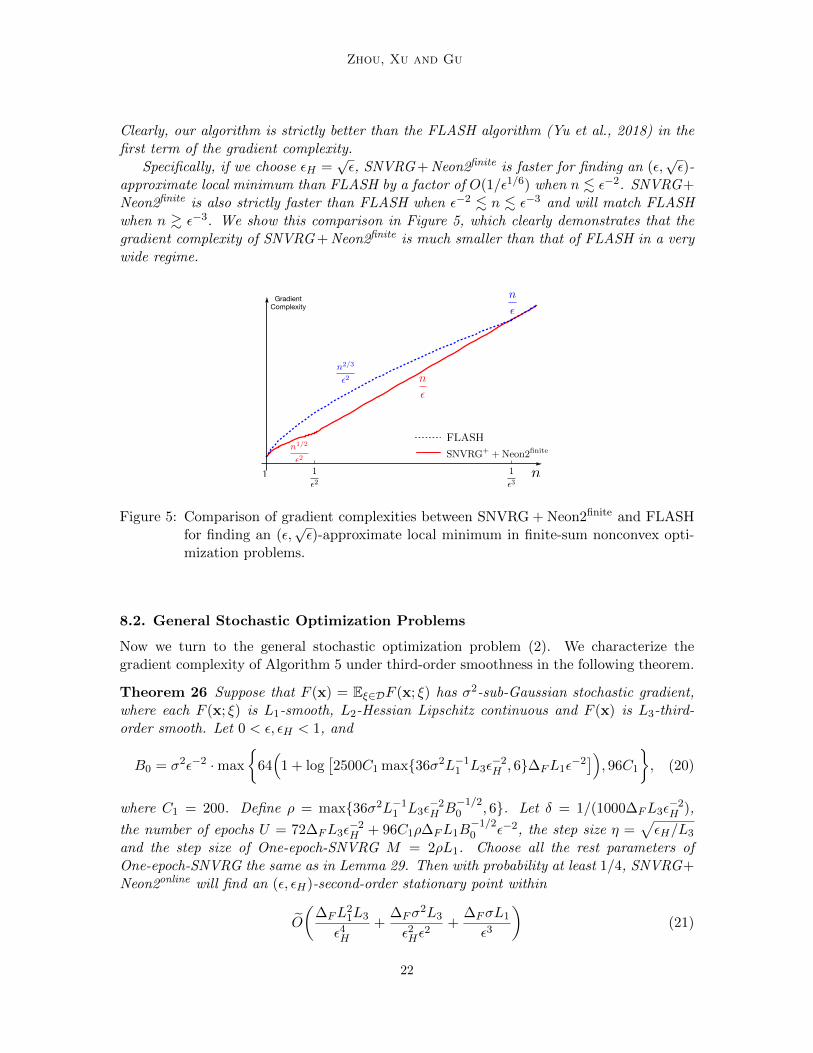
Clearly, our algorithm is strictly better than the FLASH algorithm (Yu et al., 2018) in thefirst term of the gradient complexity.
Specifically, if we choose εH =√ε, SNVRG + Neon2finite is faster for finding an (ε,
√ε)-
approximate local minimum than FLASH by a factor of O(1/ε1/6) when n . ε−2. SNVRG+Neon2finite is also strictly faster than FLASH when ε−2 . n . ε−3 and will match FLASHwhen n & ε−3. We show this comparison in Figure 5, which clearly demonstrates that thegradient complexity of SNVRG + Neon2finite is much smaller than that of FLASH in a verywide regime.
n
GradientComplexity
1
FLASHn1/2
2
n2/3
2 n
n
1
21
3
SNVRG+ + Neon2finite
Figure 5: Comparison of gradient complexities between SNVRG + Neon2finite and FLASHfor finding an (ε,
√ε)-approximate local minimum in finite-sum nonconvex opti-
mization problems.
8.2. General Stochastic Optimization Problems
Now we turn to the general stochastic optimization problem (2). We characterize thegradient complexity of Algorithm 5 under third-order smoothness in the following theorem.
Theorem 26 Suppose that F (x) = Eξ∈DF (x; ξ) has σ2-sub-Gaussian stochastic gradient,where each F (x; ξ) is L1-smooth, L2-Hessian Lipschitz continuous and F (x) is L3-third-order smooth. Let 0 < ε, εH < 1, and
B0 = σ2ε−2 ·max
64(
1 + log[2500C1 max36σ2L−1
1 L3ε−2H , 6∆FL1ε
−2]), 96C1
, (20)
where C1 = 200. Define ρ = max36σ2L−11 L3ε
−2H B
−1/20 , 6. Let δ = 1/(1000∆FL3ε
−2H ),
the number of epochs U = 72∆FL3ε−2H + 96C1ρ∆FL1B
−1/20 ε−2, the step size η =
√εH/L3
and the step size of One-epoch-SNVRG M = 2ρL1. Choose all the rest parameters ofOne-epoch-SNVRG the same as in Lemma 29. Then with probability at least 1/4, SNVRG+Neon2online will find an (ε, εH)-second-order stationary point within
O
(∆FL
21L3
ε4H+
∆Fσ2L3
ε2Hε2
+∆FσL1
ε3
)(21)
22
Stochastic Nested Variance Reduction for Nonconvex Optimization
stochastic gradient evaluations.
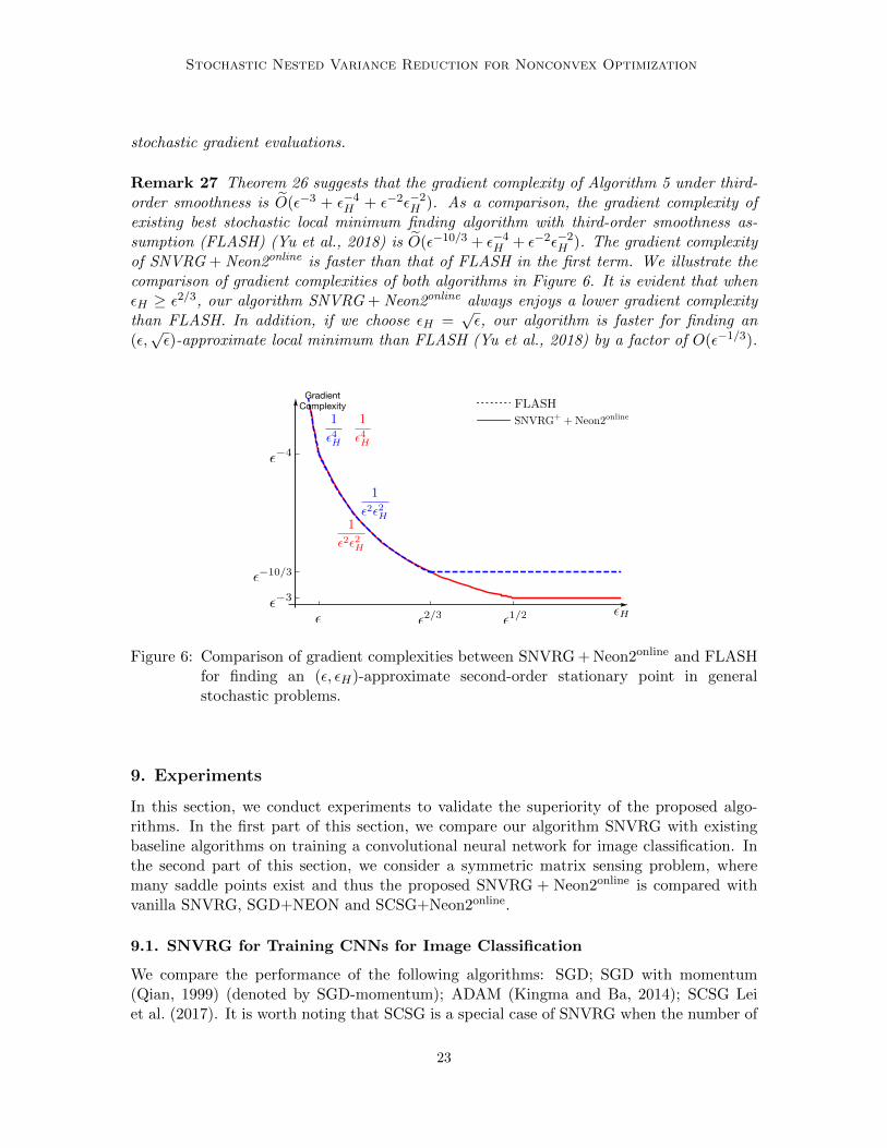
Remark 27 Theorem 26 suggests that the gradient complexity of Algorithm 5 under third-order smoothness is O(ε−3 + ε−4
H + ε−2ε−2H ). As a comparison, the gradient complexity of
existing best stochastic local minimum finding algorithm with third-order smoothness as-sumption (FLASH) (Yu et al., 2018) is O(ε−10/3 + ε−4
H + ε−2ε−2H ). The gradient complexity
of SNVRG + Neon2online is faster than that of FLASH in the first term. We illustrate thecomparison of gradient complexities of both algorithms in Figure 6. It is evident that whenεH ≥ ε2/3, our algorithm SNVRG + Neon2online always enjoys a lower gradient complexitythan FLASH. In addition, if we choose εH =
√ε, our algorithm is faster for finding an
(ε,√ε)-approximate local minimum than FLASH (Yu et al., 2018) by a factor of O(ε−1/3).
GradientComplexity
SNVRG+ + Neon2online
FLASH
H 2/3 1/23
10/3
4
1
4H
1
4H
1
22H
1
22H
Figure 6: Comparison of gradient complexities between SNVRG + Neon2online and FLASHfor finding an (ε, εH)-approximate second-order stationary point in generalstochastic problems.
9. Experiments
In this section, we conduct experiments to validate the superiority of the proposed algo-rithms. In the first part of this section, we compare our algorithm SNVRG with existingbaseline algorithms on training a convolutional neural network for image classification. Inthe second part of this section, we consider a symmetric matrix sensing problem, wheremany saddle points exist and thus the proposed SNVRG + Neon2online is compared withvanilla SNVRG, SGD+NEON and SCSG+Neon2online.
9.1. SNVRG for Training CNNs for Image Classification
We compare the performance of the following algorithms: SGD; SGD with momentum(Qian, 1999) (denoted by SGD-momentum); ADAM (Kingma and Ba, 2014); SCSG Leiet al. (2017). It is worth noting that SCSG is a special case of SNVRG when the number of
23
Zhou, Xu and Gu
nested loops K = 1. Due to the memory cost, we did not compare Gradient Descent (GD) orSVRG which need to calculate the full gradient. Although our theoretical analysis holds forgeneral K nested loops, it suffices to choose K = 2 in SNVRG to illustrate the effectivenessof the nested structure for the simplification of implementation. In this case, we have 3reference points and gradients. All experiments are conducted on Amazon AWS p2.xlargeservers which comes with Intel Xeon E5 CPU and NVIDIA Tesla K80 GPU (12G GPURAM). All algorithm are implemented in Pytorch platform version 0.4.0 within Python3.6.4.
Datasets We use three image datasets: (1) The MNIST dataset (Scholkopf and Smola,2002) consists of handwritten digits and has 50, 000 training examples and 10, 000 testexamples. The digits have been size-normalized to fit the network, and each image is 28pixels by 28 pixels. (2) CIFAR10 dataset (Krizhevsky, 2009) consists of images in 10 classesand has 50, 000 training examples and 10, 000 test examples. The digits have been size-normalized to fit the network, and each image is 32 pixels by 32 pixels. (3) SVHN datasetNetzer et al. (2011) consists of images of digits and has 531, 131 training examples and26, 032 test examples. The digits have been size-normalized to fit the network, and eachimage is 32 pixels by 32 pixels.
CNN Architecture We use the standard LeNet (LeCun et al., 1998), which has two con-volutional layers with 6 and 16 filters of size 5 respectively, followed by three fully-connectedlayers with output size 120, 84 and 10. We apply max pooling after each convolutional layer.
Implementation Details & Parameter Tuning We did not use the random data aug-mentation which is set as default by Pytorch, because it will apply random transformation(e.g., clip and rotation) at the beginning of each epoch on the original image dataset, whichwill ruin the finite-sum structure of the loss function. We set our grid search rules for allthree datasets as follows. For SGD, we search the batch size from 256, 512, 1024, 2048 andthe initial step sizes from 1, 0.1, 0.01. For SGD-momentum, we set the momentum pa-rameter as 0.9. We search its batch size from 256, 512, 1024, 2048 and the initial learningrate from 1, 0.1, 0.01. For ADAM, we search the batch size from 256, 512, 1024, 2048and the initial learning rate from 0.01, 0.001, 0.0001. For SCSG and SNVRG, we chooseloop parameters Tl which satisfy Bl ·
∏lj=1 Tj = B automatically. In addition, for SCSG,
we set the batch sizes (B,B1) = (B,B/b), where b is the batch size ratio parameter. Wesearch B from 256, 512, 1024, 2048 and we search b from 2, 4, 8. We search its initiallearning rate from 1, 0.1, 0.01. For our proposed SNVRG algorithm, we set the batchsizes (B,B1, B2) = (B,B/b,B/b2), where b is the batch size ratio parameter. We searchB from 256, 512, 1024, 2048 and b from 2, 4, 8. We search its initial learning rate from1, 0.1, 0.01.
9.1.1. Experimental Results with Learning Rate Decaying
In this section, we first present the experimental results with learning rate decay. In par-ticular, following the convention of deep learning practice, we apply learning rate decayschedule to each algorithm with the learning rate decayed by 0.1 every 20 epochs.
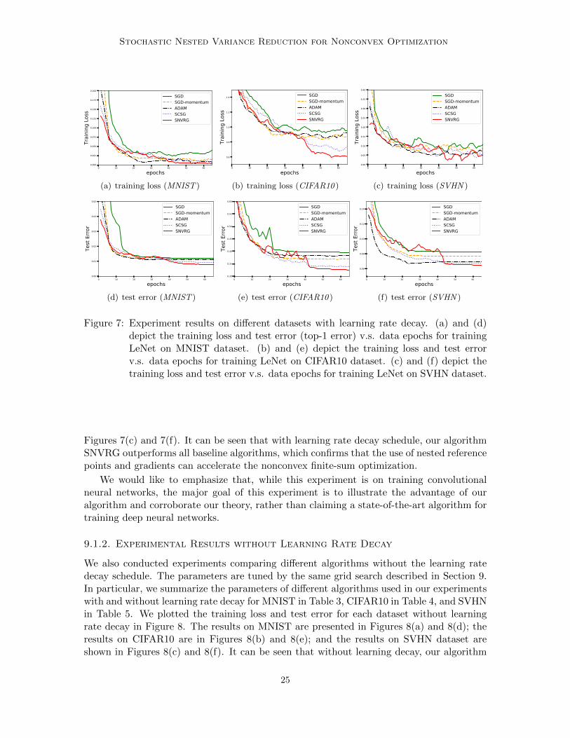
We plotted the training loss and test error for different algorithms on each dataset inFigure 7. The results on MNIST are presented in Figures 7(a) and 7(d); the results onCIFAR10 are in Figures 7(b) and 7(e); and the results on SVHN dataset are shown in
24
Stochastic Nested Variance Reduction for Nonconvex Optimization
0 10 20 30 40 50 60
epochs0.000
0.025
0.050
0.075
0.100
0.125
0.150
0.175
0.200Tr
aini
ng L
oss
SGDSGD-momentumADAMSCSGSNVRG
(a) training loss (MNIST )
0 10 20 30 40 50 60
epochs
0.6
0.8
1.0
1.2
1.4
Trai
ning
Los
s
SGDSGD-momentumADAMSCSGSNVRG
(b) training loss (CIFAR10 )
0 10 20 30 40 50 60
epochs0.00
0.05
0.10
0.15
0.20
0.25
0.30
0.35
0.40
Trai
ning
Los
s
SGDSGD-momentumADAMSCSGSNVRG
(c) training loss (SVHN )
0 10 20 30 40 50 60
epochs0.00
0.01
0.02
0.03
0.04
0.05
Test
Erro
r
SGDSGD-momentumADAMSCSGSNVRG
(d) test error (MNIST )
0 10 20 30 40 50 60
epochs0.30
0.35
0.40
0.45
0.50
0.55
0.60
Test
Erro
r
SGDSGD-momentumADAMSCSGSNVRG
(e) test error (CIFAR10 )
0 10 20 30 40 50 60
epochs
0.06
0.08
0.10
0.12
0.14
Test
Erro
r
SGDSGD-momentumADAMSCSGSNVRG
(f) test error (SVHN )
Figure 7: Experiment results on different datasets with learning rate decay. (a) and (d)depict the training loss and test error (top-1 error) v.s. data epochs for trainingLeNet on MNIST dataset. (b) and (e) depict the training loss and test errorv.s. data epochs for training LeNet on CIFAR10 dataset. (c) and (f) depict thetraining loss and test error v.s. data epochs for training LeNet on SVHN dataset.
Figures 7(c) and 7(f). It can be seen that with learning rate decay schedule, our algorithmSNVRG outperforms all baseline algorithms, which confirms that the use of nested referencepoints and gradients can accelerate the nonconvex finite-sum optimization.
We would like to emphasize that, while this experiment is on training convolutionalneural networks, the major goal of this experiment is to illustrate the advantage of ouralgorithm and corroborate our theory, rather than claiming a state-of-the-art algorithm fortraining deep neural networks.
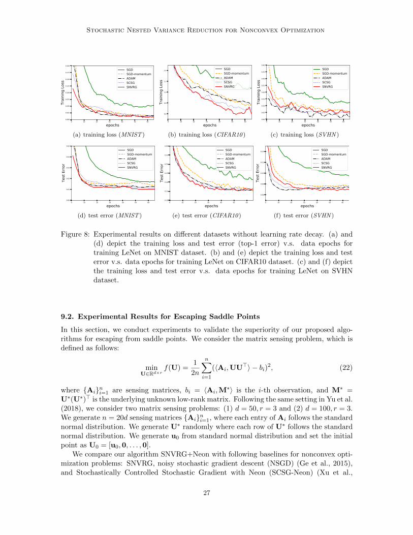
9.1.2. Experimental Results without Learning Rate Decay
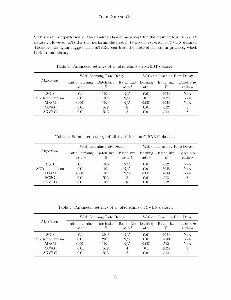
We also conducted experiments comparing different algorithms without the learning ratedecay schedule. The parameters are tuned by the same grid search described in Section 9.In particular, we summarize the parameters of different algorithms used in our experimentswith and without learning rate decay for MNIST in Table 3, CIFAR10 in Table 4, and SVHNin Table 5. We plotted the training loss and test error for each dataset without learningrate decay in Figure 8. The results on MNIST are presented in Figures 8(a) and 8(d); theresults on CIFAR10 are in Figures 8(b) and 8(e); and the results on SVHN dataset areshown in Figures 8(c) and 8(f). It can be seen that without learning decay, our algorithm
25
Zhou, Xu and Gu
SNVRG still outperforms all the baseline algorithms except for the training loss on SVHNdataset. However, SNVRG still performs the best in terms of test error on SVHN dataset.These results again suggest that SNVRG can beat the state-of-the-art in practice, whichbackups our theory.
Table 3: Parameter settings of all algorithms on MNIST dataset.
AlgorithmWith Learning Rate Decay Without Learning Rate Decay
Initial learning Batch size Batch size learning Batch size Batch sizerate η B ratio b rate η B ratio b
SGD 0.1 1024 N/A 0.01 1024 N/ASGD-momentum 0.01 1024 N/A 0.1 1024 N/A
ADAM 0.001 1024 N/A 0.001 1024 N/ASCSG 0.01 512 8 0.01 512 8
SNVRG 0.01 512 8 0.01 512 8
Table 4: Parameter settings of all algorithms on CIFAR10 dataset.
AlgorithmWith Learning Rate Decay Without Learning Rate Decay
Initial learning Batch size Batch size learning Batch size Batch sizerate η B ratio b rate η B ratio b
SGD 0.1 1024 N/A 0.01 512 N/ASGD-momentum 0.01 1024 N/A 0.01 2048 N/A
ADAM 0.001 1024 N/A 0.001 2048 N/ASCSG 0.01 512 8 0.01 512 8
SNVRG 0.01 1024 8 0.01 512 4
Table 5: Parameter settings of all algorithms on SVHN dataset.
AlgorithmWith Learning Rate Decay Without Learning Rate Decay
Initial learning Batch size Batch size learning Batch size Batch sizerate η B ratio b rate η B ratio b
SGD 0.1 2048 N/A 0.01 1024 N/ASGD-momentum 0.01 2048 N/A 0.01 2048 N/A
ADAM 0.001 1024 N/A 0.001 512 N/ASCSG 0.01 512 4 0.1 1024 4
SNVRG 0.01 512 8 0.01 512 4
26
Stochastic Nested Variance Reduction for Nonconvex Optimization
0 10 20 30 40 50 60
epochs0.000
0.025
0.050
0.075
0.100
0.125
0.150
0.175
0.200Tr
aini
ng L
oss
SGDSGD-momentumADAMSCSGSNVRG
(a) training loss (MNIST )
0 10 20 30 40 50 60
epochs
0.6
0.8
1.0
1.2
1.4
Trai
ning
Los
s
SGDSGD-momentumADAMSCSGSNVRG
(b) training loss (CIFAR10 )
0 10 20 30 40 50 60
epochs0.00
0.05
0.10
0.15
0.20
0.25
0.30
0.35
0.40
Trai
ning
Los
s
SGDSGD-momentumADAMSCSGSNVRG
(c) training loss (SVHN )
0 10 20 30 40 50 60
epochs0.00
0.01
0.02
0.03
0.04
0.05
Test
Erro
r
SGDSGD-momentumADAMSCSGSNVRG
(d) test error (MNIST )
0 10 20 30 40 50 60
epochs0.30
0.35
0.40
0.45
0.50
0.55
0.60
Test
Erro
r
SGDSGD-momentumADAMSCSGSNVRG
(e) test error (CIFAR10 )
0 10 20 30 40 50 60
epochs
0.06
0.08
0.10
0.12
0.14
Test
Erro
r
SGDSGD-momentumADAMSCSGSNVRG
(f) test error (SVHN )
Figure 8: Experimental results on different datasets without learning rate decay. (a) and(d) depict the training loss and test error (top-1 error) v.s. data epochs fortraining LeNet on MNIST dataset. (b) and (e) depict the training loss and testerror v.s. data epochs for training LeNet on CIFAR10 dataset. (c) and (f) depictthe training loss and test error v.s. data epochs for training LeNet on SVHNdataset.
9.2. Experimental Results for Escaping Saddle Points
In this section, we conduct experiments to validate the superiority of our proposed algo-rithms for escaping from saddle points. We consider the matrix sensing problem, which isdefined as follows:
minU∈Rd×r
f(U) =1
2n
n∑
i=1
(〈Ai,UU>〉 − bi)2, (22)
where Aini=1 are sensing matrices, bi = 〈Ai,M∗〉 is the i-th observation, and M∗ =
U∗(U∗)> is the underlying unknown low-rank matrix. Following the same setting in Yu et al.(2018), we consider two matrix sensing problems: (1) d = 50, r = 3 and (2) d = 100, r = 3.We generate n = 20d sensing matrices Aini=1, where each entry of Ai follows the standardnormal distribution. We generate U∗ randomly where each row of U∗ follows the standardnormal distribution. We generate u0 from standard normal distribution and set the initialpoint as U0 = [u0,0, . . . ,0].
We compare our algorithm SNVRG+Neon with following baselines for nonconvex opti-mization problems: SNVRG, noisy stochastic gradient descent (NSGD) (Ge et al., 2015),and Stochastically Controlled Stochastic Gradient with Neon (SCSG-Neon) (Xu et al.,
27
Zhou, Xu and Gu
0.0 0.5 1.0 1.5 2.0 2.5
time in seconds
10 4
10 3
10 2
10 1
100Fu
nctio
n Va
lue
Gap
SNVRGNSGDSCSG+NeonSNVRG+Neon
(a) d = 50, r = 3
0.0 2.5 5.0 7.5 10.0 12.5 15.0 17.5
time in seconds
10 4
10 3
10 2
10 1
100
Func
tion
Valu
e Ga
p
SNVRGNSGDSCSG+NeonSNVRG+Neon
(b) d = 100, r = 3
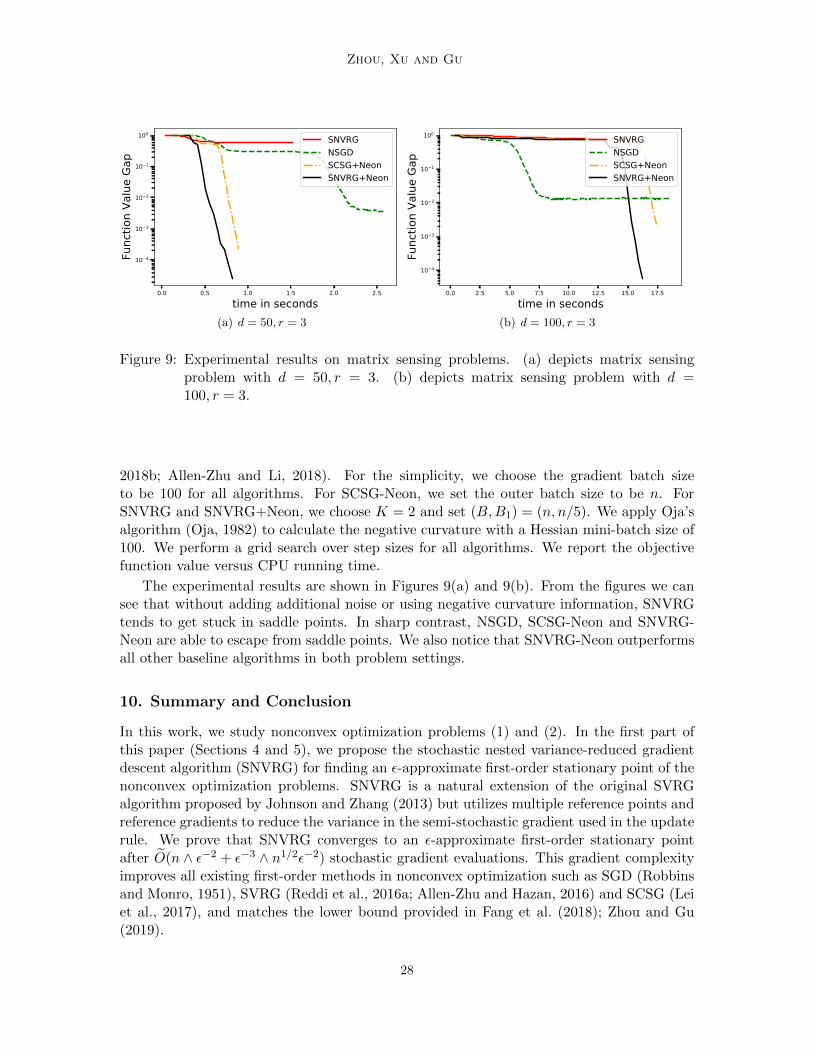
Figure 9: Experimental results on matrix sensing problems. (a) depicts matrix sensingproblem with d = 50, r = 3. (b) depicts matrix sensing problem with d =100, r = 3.
2018b; Allen-Zhu and Li, 2018). For the simplicity, we choose the gradient batch sizeto be 100 for all algorithms. For SCSG-Neon, we set the outer batch size to be n. ForSNVRG and SNVRG+Neon, we choose K = 2 and set (B,B1) = (n, n/5). We apply Oja’salgorithm (Oja, 1982) to calculate the negative curvature with a Hessian mini-batch size of100. We perform a grid search over step sizes for all algorithms. We report the objectivefunction value versus CPU running time.
The experimental results are shown in Figures 9(a) and 9(b). From the figures we cansee that without adding additional noise or using negative curvature information, SNVRGtends to get stuck in saddle points. In sharp contrast, NSGD, SCSG-Neon and SNVRG-Neon are able to escape from saddle points. We also notice that SNVRG-Neon outperformsall other baseline algorithms in both problem settings.
10. Summary and Conclusion
In this work, we study nonconvex optimization problems (1) and (2). In the first part ofthis paper (Sections 4 and 5), we propose the stochastic nested variance-reduced gradientdescent algorithm (SNVRG) for finding an ε-approximate first-order stationary point of thenonconvex optimization problems. SNVRG is a natural extension of the original SVRGalgorithm proposed by Johnson and Zhang (2013) but utilizes multiple reference points andreference gradients to reduce the variance in the semi-stochastic gradient used in the updaterule. We prove that SNVRG converges to an ε-approximate first-order stationary pointafter O(n ∧ ε−2 + ε−3 ∧ n1/2ε−2) stochastic gradient evaluations. This gradient complexityimproves all existing first-order methods in nonconvex optimization such as SGD (Robbinsand Monro, 1951), SVRG (Reddi et al., 2016a; Allen-Zhu and Hazan, 2016) and SCSG (Leiet al., 2017), and matches the lower bound provided in Fang et al. (2018); Zhou and Gu(2019).
28
Stochastic Nested Variance Reduction for Nonconvex Optimization
In the second part of this paper (Sections 6, 7 and 8), we integrate SNVRG with re-cently proposed NEON/Neon2 algorithms (Xu et al., 2018b; Allen-Zhu and Li, 2018) andpropose a class of algorithms that can find local minima, i.e., (ε,
√ε)-approximate second-
order stationary points of the nonconvex optimization problems. The proposed algorithmsSNVRG + Neon2finite and SNVRG + Neon2online achieve the state-of-the-art gradient com-plexities for finding local minima in nonconvex optimization. Detailed comparison is pre-sented in Table 2. Furthermore, we provide an alternative analysis of these two algo-rithms when the objective function enjoys the third-order smoothness property (Anandku-mar and Ge, 2016; Carmon et al., 2017; Yu et al., 2018). With this property, we prove thatSNVRG + Neon2finite and SNVRG + Neon2online attain lower gradient complexities and canfind local minima more efficiently.
Acknowledgement
We would like to thank the anonymous reviewers for their helpful comments. This re-search was sponsored in part by the National Science Foundation BIGDATA IIS-1855099,IIS-1904183 and IIS-1906169. We also thank AWS for providing cloud computing creditsassociated with the NSF BIGDATA award. The views and conclusions contained in thispaper are those of the authors and should not be interpreted as representing any fundingagencies.
Appendix A. Proof of Main Theory for Finding Stationary Points
In this section, we provide the proofs of our theoretical analysis in Section 5 for findingfirst-order stationary points.
A.1. Proof of Theorem 12
We start with the following supporting lemma that characterizes the function value decreaseof One-epoch-SNVRG (Algorithm 1).
Lemma 28 Suppose that F has averaged L-Lipschitz gradient. Suppose that B0 ≥ 4 andthe rest parameters (K,M, Bl, Tl) of Algorithm 1 are chosen the same as in (12). ThenAlgorithm 1 with Option I satisfies
E‖∇F (xout)‖22 ≤ C(
L
B1/20
· E[F (x0)− F (xT )
]+σ2
B0· 1(B0 < n)
)(23)
within 1 ∨ (10B0 log3B0) stochastic gradient computations, where T =∏Kl=1 Tl, C = 6000
is a constant and 1(·) is the indicator function.
Now we prove our main theorem which spells out the gradient complexity of SNVRG.
Proof [Proof of Theorem 12] By (23) we have
E‖∇F (ys)‖22 ≤ C(
L
B1/20
· E[F (zs−1)− F (zs)
]+σ2
B0· 1(B0 < n)
), (24)
29
Zhou, Xu and Gu
where C = 6000. Taking summation for (24) over s from 1 to S, we have
S∑
s=1
E‖∇F (ys)‖22 ≤ C(
L
B1/20
· E[F (z0)− F (zS)
]+σ2
B0· 1(B0 < n) · S
). (25)
Dividing both sides of (25) by S, we immediately obtain
E‖∇F (yout)‖22 ≤ C(LE[F (z0)− F ∗
]
SB1/20
+σ2
B0· 1(B0 < n)
)(26)
= C
(L∆F
SB1/20
+σ2
B0· 1(B0 < n)
), (27)
where (26) holds because F (zS) ≥ F ∗ and by the definition ∆F = F (z0)−F ∗. By the choice
of parameters in Theorem 12, we have B0 = n ∧ (2Cσ2/ε2), S = 1 ∨ (2CL∆F /(B1/20 ε2)),
which implies
1(B0 < n) · σ2/B0 ≤ ε2/(2C), and L∆F /(SB1/20 ) ≤ ε2/(2C). (28)
Submitting (28) into (27), we have E‖∇F (yout)‖22 ≤ 2Cε2/(2C) = ε2. By Lemma 23, wehave that each One-epoch-SNVRG takes less than 7B0 log3B0 stochastic gradient compu-tations. Since we have total S epochs, so the total gradient complexity of Algorithm 2 isless than
S · 7B0 log3B0 ≤ 7B0 log3B0 +L∆F
ε2· 7B1/2
0 log3B0
= O
(log3
(σ2
ε2∧ n)[
σ2
ε2∧ n+
L∆F
ε2
[σ2
ε2∧ n]1/2])
,
which leads to the conclusion.
A.2. Proof of Theorem 14
We then prove the main theorem on gradient complexity of SNVRG under gradient domi-nance condition (Algorithm 3).Proof [Proof of Theorem 14] Following the proof of Theorem 12, we obtain a similarinequality with (26):
E‖∇F (zu+1)‖22 ≤ C(LE[F (zu)− F ∗]
SB1/20
+σ2
B0· 1(B0 < n)
). (29)
Since F is a τ -gradient dominated function, we have E‖∇F (zu+1)‖22 ≥ 1/τ ·E[F (zu+1)−F ∗]by Definition 9. Plugging this inequality into (29) yields
E[F (zu+1)− F ∗
]≤ CτL
SB1/20
· E[F (zu)− F ∗
]+Cτσ2
B0· 1(B0 < n)
30
Stochastic Nested Variance Reduction for Nonconvex Optimization
≤ 1
2E[F (zu)− F ∗
]+ε
4, (30)
where the second inequality holds due to the choice of parameters B0 = n∧ (4C1τσ2/ε) and
S = 1 ∨ (2C1τL/B1/20 ) for Algorithm 3 in Theorem 14. By (30) we can derive
E[F (zu+1)− F ∗
]− ε
2≤ 1
2
(E[F (zu)− F ∗
]− ε
2
),
which immediately implies
E[F (zU )− F ∗
]− ε
2≤ 1
2U
(∆F −
ε
2
)≤ ∆F
2U. (31)
Plugging the number of epochs U = log(2∆F /ε) into (31), we obtain E[F (zU ) − F ∗
]≤ ε.
Note that each epoch of Algorithm 3 needs at most S · 7B0 log3B0 stochastic gradient com-putations by Theorem 12 and Algorithm 3 has U epochs, which implies the total stochasticgradient complexity
U · S · 7B0 log3B0 = O
(log3
(n ∧ τσ
2
ε
)log
∆F
ε
[n ∧ τσ
2
ε+ τL
[n ∧ τσ
2
ε
]1/2]),
which completes the proof.
Appendix B. Proof of Main Theory for Finding Local Minima
In this section, we provide the proofs of gradient complexities of our proposed algorithmsSNVRG + Neon2finite and SNVRG + Neon2online.
B.1. Proof of Theorem 18
It is worth noting that in order to find local minima we apply One-epoch-SNVRG withOption II which samples the total number of epochs T from a geometric distribution. Similarto the analysis for finding first-order stationary points, we also have the following supportinglemma about the function value decrease of Algorithm 1.
Lemma 29 Suppose that each fi is L1-smooth and F has σ2-sub-Gaussian stochastic gra-dient. In Algorithm 1, suppose that B0 ≥ 4 and the rest parameters (K,M, Bl, Tl) ofAlgorithm 1 are chosen the same as in (12). Then Algorithm 1 with Option II satisfies
E‖∇F (xT )‖22 ≤ C(
M
B1/20
· E[F (x0)− F (xT )] +2σ2
B0· 1B0 < n
), (32)
where C = 1000. In addition, the total number of stochastic gradient computations T byAlgorithm 1 satisfies ET ≤ 10B0 log3B0.
31
Zhou, Xu and Gu
Remark 30 Note that Lemma 28 is regarding xout, which is a uniformly chosen iterate fromx1, . . . ,xT . In contrast, Lemma 29 is regarding the last iterate of xT in Algorithm 1. Thisdifference leads to the nonergodic-type and ergodic-type guarantees of One-epoch-SNVRGwhich plays different roles in the analysis of stationary point finding algorithms and localminimum finding algorithms.
Remark 31 For simplicity, we use ∇fi(x) to denote the stochastic gradient at point xin our One-epoch-SNVRG algorithm (Lines 20 and 23 in Algorithm 1) and the analysisof Lemma 29. However, we emphasize that One-epoch-SNVRG also works in the generalstochastic optimization setting if we replace ∇fi(x) with ∇F (x; ξi) for any index i. And thetheoretical result in Lemma 29 still holds.
When F (x) has the finite-sum structure in (1), we choose B0 = n,M = 6L1 inOne-epoch-SNVRG. Lemma 29 straightforwardly implies the following corollary.
Corollary 32 Suppose that each fi is L1-smooth. We choose B0 = n, and let other pa-rameters be chose as in Lemma 29. Then the output of Algorithm 1 with Option II satisfies
E‖∇F (xT )‖22 ≤CL1
n1/2· E[F (x0)− F (xT )
],
where C = 6000. Let T be the total amount of stochastic gradient computations of Algorithm1, then we have ET ≤ 10n log3 n.
The following lemma shows that based on Neon2finite the negative curvature descent stepof Algorithm 4 (Line 12) enjoys sufficient function value decrease. The proof can be foundin Theorem 5 and Claim C.2 in Allen-Zhu and Li (2018).
Lemma 33 (Allen-Zhu and Li (2018)) Suppose that F = 1/n∑n
i=1 fi, each fi is L1-smooth and L2-Hessian Lipschitz continuous. Let εH ∈ (0, 1) and set η = εH/L2. Sup-pose that λmin(∇2F (zu−1)) < −εH and that at the u-th iteration Algorithm 4 executes theNeon2finite algorithm (Line 7). Then with probability 1− δ it holds that
Eζ[F (zu)− F (zu−1)
]≤ −ε3H/(12L2
2).
In addition, Neon2finite takes O((n+ n3/4
√L1/εH) log2(d/δ)
)stochastic gradient computa-
tions.
Proof [Proof of Theorem 18] Let I = 1, . . . , U be the index set of all iterations. Wedenote I1 and I2 as the index sets such that zu is obtained from Neon2finite for all u ∈ I1
and zu′ is the output by SNVRG for all u′ ∈ I2. Obviously we have U = |I1| + |I2|. Wewill calculate |I1|, |I2| separately. For |I1|, by Lemma 33, with probability 1− δ, we have
E[F (zu)− F (zu−1)
]≤ −ε3H/(12L2
2), for u ∈ I1. (33)
Summing up (33) over u ∈ I1, then with probability 1− δ · |I1| we have
|I1| · ε3H/(12L22) ≤
∑
u∈I1
E[F (zu−1)− F (zu)
]≤∑
u∈IE[F (zu−1)− F (zu)
]≤ ∆F , (34)
32
Stochastic Nested Variance Reduction for Nonconvex Optimization
where the second inequality holds because by Corollary 32 it holds that
0 ≤ E‖∇F (zu)‖22 ≤CL1
n1/2E[F (zu−1)− F (zu)
], for all u ∈ I2. (35)
By (34), we have
|I1| ≤ 12L22∆F /ε
3H .
To calculate |I2|, we further decompose I2 into two disjoint sets such that I2 = I12 ∪ I2
2 ,where I1
2 = u ∈ I2 : ‖gu‖2 > ε, I22 = u ∈ I2 : ‖gu‖2 ≤ ε. It is worth noting that
if u ∈ I22 such that ‖gu‖2 ≤ ε, then Algorithm 4 will execute Neon2finite and a negative
curvature descent step, which means u + 1 ∈ I1 by definition. Thus, it always holds that|I2
2 | ≤ |I1|. For |I12 |, note that x0 = zu−1 and xT = zu in Corollary 32, which directly
implies
∑
u∈I12
E‖∇F (zu)‖22 ≤∑
u∈I12
CL1
n1/2E[F (zu−1)− F (zu)
]
≤∑
u∈I
CL1
n1/2E[F (zu−1)− F (zu)
]
≤ CL1
n1/2·∆F , (36)
where the second inequality holds because E[F (zu−1)− F (zu)] ≥ 0 for u ∈ I1 ∪ I2 by (33)and (35). Applying Markov’s inequality, with probability at least 2/3, we have
∑
u∈I12
‖∇F (zu)‖22 ≤3CL1∆F
n1/2.
Since for any u ∈ I12 , we have ‖∇F (zu)‖2 = ‖gu‖2 > ε, with probability at least 2/3 it
holds that
|I12 | ≤
3CL1∆F
ε2n1/2.
Thus, the total number of iterations is U = |I1| + |I2| ≤ 2|I1| + |I12 | ≤ 24L2
2∆F ε−3H +
3CL1∆F ε−2n−1/2.
We now calculate the gradient complexity of Algorithm 4. By Corollary 32 one singlecall of One-epoch-SNVRG needs at most 20n log3 n stochastic gradient computations andby Lemma 33 one single call of Neon2finite needs O
((n+n3/4
√L1/εH) log2(d/δ)
)stochastic
gradient computations. In addition, we need to compute gu at each iteration of Algorithm4 (Line 3), which takes O(n) stochastic gradient computations. Thus, the expectation ofthe total amount of stochastic gradient computations, denoted by ETtotal, can be upperbounded by
|I1| ·O((n+ n3/4
√L1/εH) log2(d/δ)
)+ |I2| ·O(n log3 n) + |I| ·O(n)
= |I1| · O(n+ n3/4
√L1/εH
)+ (|I1
2 |+ |I22 |) · O(n)
33
Zhou, Xu and Gu
= |I1| · O(n+ n3/4
√L1/εH
)+ (|I1
2 |+ |I1|) · O(n). (37)
We further plug the upper bound for |I1| and |I12 | into (37) and obtain
ETtotal = O(L22∆F ε
−3H ) · O
(n+ n3/4
√L1/εH
)+O(L1∆F ε
−2n−1/2)O(n)
= O(∆FnL
22ε−3H + ∆Fn
3/4L1/21 L2
2ε−7/2H + ∆Fn
1/2L1ε−2).
Finally, applying Markov inequality, with probability 2/3, it holds that
Ttotal = O(∆FnL
22ε−3H + ∆Fn
3/4L1/21 L2
2ε−7/2H + ∆Fn
1/2L1ε−2).
Since |I1|δ = |I1|/(144 · L22∆F ε
−3H ) ≤ 1/12, then by the union bound, with probability
1−1/3−1/3−|I1|δ ≥ 1/4, SNVRG+Neon2finite will find an (ε, εH)-second order stationarypoint within
O(∆FnL
22ε−3H + ∆Fn
3/4L1/21 L2
2ε−7/2H + ∆Fn
1/2L1ε−2)
stochastic gradient computations.
B.2. Proof of Theorem 21
For general stochastic problem in (2), we denote ∇F (x; ξi) as one subsampled gradient at xfor any random variable ξ and index i in One-epoch-SNVRG. Base on Lemma 28 we havethe next corollary.
Corollary 34 Suppose that for each ξ, F (x; ξ) is L1-smooth and has σ2-sub-Gaussianstochastic gradient. We choose M = 2ρL1 and suppose that n O(ε−2) and B0 < n.Then the output of Algorithm 1 with Option II satisfies
E‖∇F (xT )‖22 ≤ C1
(ρL1
B1/20
· E[F (x0)− F (xT )
]+σ2
B0
),
where C1 = 2000. The total amount of stochastic gradient computations of Algorithm 1 isET ≤ 20B0 log3B0.
The following lemma shows that based on Neon2online the negative curvature descent stepof Algorithm 5 (Line 13) enjoys sufficient function value decrease. More detailed aboutNeon2online can be found in Algorithm 7. The proof can be found as a combination ofTheorem 1, Lemma 3.1 and Claim C.2 in Allen-Zhu and Li (2018).
Lemma 35 (Allen-Zhu and Li (2018)) Suppose that F (x) = Eξ∈DF (x; ξ) and each F (x; ξ)is L1-smooth, L2-Hessian Lipschitz continuous. Let εH ∈ (0, 1) and set η = εH/L2. Sup-pose that λmin(∇2F (zu−1)) < −εH and that at the u-th iteration Algorithm 5 executes theNeon2online algorithm (Line 8). Then with probability 1− δ it holds that
Eζ[F (zu)− F (zu−1)
]≤ −ε3H/(12L2
2).
In addition, Neon2online takes O(L21/ε
2H log2(d/δ)) stochastic gradient computations.
34
Stochastic Nested Variance Reduction for Nonconvex Optimization
We also need the following concentration inequality in our proof.
Lemma 36 (Ghadimi et al. (2016)) Suppose the stochastic gradient ∇F (x; ξ) is σ2-sub-Gaussian. Let ∇FS(x) = 1/|S|∑i∈S ∇F (x; ξi), where S is a subsampled gradient of
F (x). If the sample size satisfies |S| = 2σ2/ε2(1 + log1/2(1/δ))2, then with probability atleast 1− δ,
‖∇FS(x)−∇F (x)‖2 ≤ ε.
Proof [Proof of Theorem 21] Denote δ0 = 1/(2500C1ρ∆FL1B−1/20 ε−2). Then by the choice
of B0 in (17) it holds that B0 > 32σ2/ε2(1+log1/2(1/δ0))2. Let I = 1, . . . , U be the indexset of all iterations. We use I1 and I2 to represent the index set of iterates where the zuis obtained from Neon2finite and SNVRG respectively. From Lemma 35, we have that withprobability at least 1− δ that
E[F (zu)− F (zu−1)
]≤ −ε3H/(12L2
2), for u ∈ I1. (38)
By Corollary 34, we have
E‖∇F (zu)‖22 ≤ C1
(ρL1
B1/20
· E[F (zu−1)− F (zu)
]+σ2
B0
), for u ∈ I2. (39)
where C1 = 200. We further decompose I2 = I12 ∪ I2
2 , where I12 = u ∈ I2 : ‖gu‖2 > ε/2
and I12 = u ∈ I2 : ‖gu‖2 ≤ ε/2. (39) immediately implies the following two inequalities:
E[F (zu)− F (zu−1)
]≤ − B
1/20
C1ρL1E‖∇F (zu)‖22 +
σ2
ρL1B1/20
, u ∈ I12 , (40)
E[F (zu)− F (zu−1)
]≤ σ2
ρL1B1/20
, u ∈ I22 . (41)
Summing up (38) over u ∈ I1, (40) over u ∈ I12 and (41) over u ∈ I2
2 , we have
E[∑
u∈IF (zu−1)− F (zu)
]≥ |I1|ε3H
12L22
+B
1/20
C1ρL1
∑
u∈I12
E‖∇F (zu)‖22
−∑
u∈I12
σ2
ρL1B1/20
−∑
u∈I22
σ2
ρL1B1/20
. (42)
Since for any u ∈ I22 we have ‖gu‖2 ≤ ε/2, Algorithm 5 will execute Neon2online at the u-th
iteration, which indicates |I22 | ≤ |I1|. Combining this with (42) and by the definition of
∆F , with probability at least 1− |I1|δ, we have
|I1|ε3H12L2
2
+B
1/20
C1ρL1
∑
u∈I12
E‖∇F (zu)‖22 ≤ ∆F + (|I1|+ |I12 |)
σ2
ρL1B1/20
. (43)
35
Zhou, Xu and Gu
Using Markov inequality, then with probability at least 2/3, it holds that
|I1|ε3H12L2
2
+B
1/20
C1ρL1
∑
u∈I12
‖∇F (zu)‖22 ≤ 3
(∆F + (|I1|+ |I1
2 |)σ2
ρL1B1/20
). (44)
By Lemma 36, for any u ∈ I12 , with probability at least 1−δ0, it holds that ‖∇F (zu)−gu‖2 <
ε/4 if B0 ≥ 32σ2/ε2(1+log1/2(1/δ0))2, which further indicates that ‖∇F (zu)‖2 > ε/4. Thus,applying union bound yields that with probability at least 1− |I1|δ − 1/3− |I1
2 |δ0 we have
|I1|ε3H12L2
2
+|I1
2 |B1/20 ε2
16C1ρL1≤ 3∆F +
3|I12 |σ2
ρL1B1/20
+3|I1|σ2
ρL1B1/20
. (45)
Recall that in Theorem 21 we set ρ = max54σ2L−11 L2
2ε−3H B
−1/20 , 6 ≥ 54σ2L2
2/(L1ε3HB
1/20 ),
which implies
3|I1|σ2
ρL1B1/20
≤ |I1|ε3H18L2
2
. (46)
By (17) we have B0 > 96C1σ2ε−2, which implies
3|I12 |σ2
ρL1B1/20
≤ |I12 |B
1/20 ε2
32C1ρL1. (47)
Plugging (46) and (47) into (45) and rearranging the resulting inequality, then with prob-ability 1− |I1|δ − 1/3− |I1
2 |δ0, we have
|I1|ε3H36L2
2
+|I1
2 |B1/20 ε2
32C1ρL1≤ 3∆F ,
which immediately implies that
|I1| ≤ 108∆FL22ε−3H = O(∆FL
22ε−3H ), (48)
and
|I12 | ≤ 96C1ρ∆FL1B
−1/20 ε−2
= max54σ2L−11 L2
2ε−3H B
−1/20 , 6 · 96C1∆FL1B
−1/20 ε−2
= O(∆Fσ−1L1ε
−1) + O(∆FL22ε−3H ). (49)
Thus we can calculate U = |I1|+ |I2| ≤ 2|I1|+ |I12 | ≤ 216∆FL
22ε−3H +96C1ρ∆FL1B
−1/20 ε−2.
Now we are ready to calculate the gradient complexity of Algorithm 5. By Lemma 35,we know that one single call of Neon2online needs O
(L2
1/ε2H log2(d/δ)
)stochastic gradient
computations, and one single call of One-epoch-SNVRG needs 20B0 log3B0 = O(σ2/ε2)stochastic gradient computations. In addition, we need to compute gu at each iteration of
36
Stochastic Nested Variance Reduction for Nonconvex Optimization
Algorithm 5 (Line 3), which costs B0 = O(σ2/ε2) stochastic gradient computations. Thus,the expected total amount of stochastic gradient computations ETtotal can be bounded as
ETtotal = |I1| ·O(L21/ε
2H log2(d/δ)) + |I2| · O(σ2/ε2) + |I| · O(σ2/ε2)
= |I1| · O(L21/ε
2H) + (|I1
2 |+ |I22 |) · O(σ2/ε2) + |I| · O(σ2/ε2)
= |I1| · O(L21/ε
2H) + (|I1
2 |+ |I1|) · O(σ2/ε2)
= O(∆FL21L
22ε−5H + ∆Fσ
2L22ε−3H ε−2 + ∆FσL1ε
−3).
Applying Markov inequality yields
Ttotal = O(∆FL21L
22ε−5H + ∆Fσ
2L22ε−3H ε−2 + ∆FσL1ε
−3)
with probability at least 2/3. Furthermore, we have |I1|δ = |I1|/(3000∆FL22ε−3H ) ≤ 1/24
and |I12 |δ0 = |I1
2 |/(2500C1ρ∆FL1B−1/20 ε−2) < 1/24. Therefore, with probability at least
1−|I1|δ−1/3−|I12 |δ0−1/3 ≥ 1/4, Algorithm 5 can find an (ε, εH)-second order stationary
point within
O(∆FL21L
22ε−5H + ∆Fσ
2L22ε−3H ε−2 + ∆FσL1ε
−3)
stochastic gradient computations.
Appendix C. Proof of Main Theory with Third-order Smoothness
In this section, we prove the theoretical results of our proposed algorithms under third-ordersmoothness condition.
C.1. Proof of Theorem 23
The following lemma shows that the negative curvature descent step (Line 12) of Algorithm4 achieves more function value decrease under third-order smoothness assumption. Theproof can be found in Lemma 4.3 of Yu et al. (2018).
Lemma 37 (Yu et al. (2018)) Suppose that F = 1/n∑n
i=1 fi, each fi is L1-smooth, L2-Hessian Lipschitz continuous and F is L3-third-order smooth. Let εH ∈ (0, 1) and η =√
3εH/L3. Suppose that λmin(∇2F (zu−1)) < −εH and that at the u-th iteration Algorithm4 executes the Neon2finite algorithm (Line 7). Then with probability 1− δ it holds that
Eζ[F (zu)− F (zu−1)
]≤ −ε2H/(6L3).
In addition, Neon2finite takes O((n+ n3/4
√L1/εH) log2(d/δ)
)stochastic gradient computa-
tions.
Proof [Proof of Theorem 23] Denote I = 1, . . . , U as the index of iteration. Let I =1, . . . , U be the index set of iteration. We use I1 and I2 to represent the index set ofiterates where the zu is obtained from Neon2finite and One-epoch-SNVRG. Since U =
37
Zhou, Xu and Gu
|I1| + |I2|, we calculate |I1|, |I2| separately. For |I1|, by Lemma 37, with probability atleast 1− δ, we have
E[F (zu)− F (zu−1)
]≤ −ε2H/(6L3), for u ∈ I1. (50)
Summing up (50) over u ∈ I1 and applying union bound, then with probability at least1− δ · |I1| we have
|I1| · ε2H/(6L3) ≤∑
u∈I1
E[F (zu−1)− F (zu)
]≤∑
u∈IE[F (zu−1)− F (zu)
]≤ ∆F , (51)
where the second inequality holds due to the fact that by Corollary 32 we have
0 ≤ E‖∇F (zu)‖22 ≤CL1
n1/2E[F (zu−1)− F (zu)
], for u ∈ I2. (52)
(51) directly implies
|I1| ≤ 6L3∆F /ε2H .
For |I2|, we decompose I2 = I12 ∪ I2
2 , where I12 = u ∈ I2 : ‖gu‖2 > ε and I2
2 = u ∈ I2 :‖gu‖2 ≤ ε. If u ∈ I2
2 , then at the (u+ 1)-th iteration, Algorithm 4 will execute Neon2finite.Thus, we have |I2
2 | ≤ |I1|. For |I12 |, note that x0 = zu−1 and xT = zu in Corollary 32 and
summing up over u ∈ I12 yields
∑
u∈I12
E‖∇F (zu)‖22 ≤∑
u∈I12
CL1
n1/2E[F (zu−1)− F (zu)
]
≤∑
u∈I
CL1
n1/2E[F (zu−1)− F (zu)
]
≤ CL1
n1/2·∆F , (53)
where the second inequality follows from (51) and (52). Applying Markov’s inequality, withprobability at least 2/3, we have
∑
u∈I12
‖∇F (zu)‖22 ≤3CL1∆F
n1/2.
by definition for any u ∈ I12 , we have ‖∇F (zu)‖2 = ‖gu‖2 > ε. Then we have with
probability at least 2/3 that
|I12 | ≤
3CL1∆F
ε2n1/2.
Total number of iteration is U = |I1|+ |I2| ≤ 2|I1|+ |I12 | ≤ 12L3∆F ε
−2H +3CL1∆F ε
−2n−1/2.We now calculate the gradient complexity of Algorithm 4. By Lemma 37 one single call ofNeon2finite needs O
((n+ n3/4
√L1/εH) log2(d/δ)
)stochastic gradient computations and by
38
Stochastic Nested Variance Reduction for Nonconvex Optimization
Corollary 32 one single call of One-epoch-SNVRG needs 20n log3 n stochastic gradient com-putations. Moreover, we need to compute gu at each iteration, which takes O(n) stochasticgradient computations. Thus, the expectation of the total amount of stochastic gradientcomputations ETtotal can be bounded by
|I1| ·O((n+ n3/4
√L1/εH) log2(d/δ)
)+ |I2| ·O(n log3 n) + |I| ·O(n)
= |I1| · O(n+ n3/4
√L1/εH
)+ (|I1
2 |+ |I22 |) · O(n)
= |I1| · O(n+ n3/4
√L1/εH
)+ (|I1
2 |+ |I1|) · O(n). (54)
We further plug the upper bound of |I1| and |I12 | into (54) and obtain
ETtotal = O(L3∆F ε−2H ) · O
(n+ n3/4
√L1/εH
)+O(L1∆F ε
−2n−1/2)O(n)
= O(∆FnL3ε
−2H + ∆Fn
3/4L1/21 L3ε
−5/2H + ∆Fn
1/2L1ε−2).
Using Markov inequality, with probability at least 2/3, we have
Ttotal = O(∆FnL3ε
−2H + ∆Fn
3/4L1/21 L3ε
−5/2H + ∆Fn
1/2L1ε−2).
Note that |I1|δ = |I1|/(72 · L3∆F ε−2H ) ≤ 1/12. By union bound, with probability at least
1−1/3−1/3−|I1|δ ≥ 1/4, SNVRG+Neon2finite will find an (ε, εH)-second order stationarypoint within
O(∆FnL3ε
−2H + ∆Fn
3/4L1/21 L3ε
−5/2H + ∆Fn
1/2L1ε−2)
stochastic gradient computations.
C.2. Proof of Theorem 26
The following lemma shows that the negative curvature descent step (Line 13) of Algorithm5 achieves more function value decrease under third-order smoothness assumption. Theproof can be found in Lemma 4.6 of Yu et al. (2018).
Lemma 38 (Yu et al. (2018)) Suppose that F (x) = Eξ∈DF (x; ξ), each F (x; ξ) is L1-smooth, L2-Hessian Lipschitz continuous and F (x) is L3-third-order smooth. Let εH ∈ (0, 1)and η =
√3εH/L3. Suppose that λmin(∇2F (zu−1)) < −εH and that at the u-th iteration
Algorithm 5 executes the Neon2online algorithm (Line 8). Then with probability 1−δ it holdsthat
Eζ[F (zu)− F (zu−1)
]≤ −ε2H/(6L3).
In addition, Neon2online takes O(L21/ε
2H log2(d/δ)) stochastic gradient computations.
Proof [Proof of Theorem 26] Denote δ0 = 1/(2500C1ρ∆FL1B−1/20 ε−2), then by (20) we
have B0 > 32σ2/ε2(1 + log1/2(1/δ0))2. Let I = 1, . . . , U be the index set of all iterations.We use I1 and I2 to represent the index set of iterates where zu is obtained from Neon2online
39
Zhou, Xu and Gu
and One-epoch-SNVRG respectively. Obviously U = |I1|+|I2| and we need to upper bound|I1| and |I2|. From Lemma 38, we have with probability at least 1− δ that
E[F (zu)− F (zu−1)
]≤ −ε2H/(6L3), for u ∈ I1. (55)
By Corollary 34, we have
E‖∇F (zu)‖22 ≤ C1
(ρL1
B1/20
· E[F (zu−1)− F (zu)
]+σ2
B0
), for u ∈ I2, (56)
where C1 = 200. We decompose I2 into two disjoint sets I2 = I12 ∪ I2
2 , where I12 = u ∈
I2 : ‖gu‖2 > ε/2 and I12 = u ∈ I2 : ‖gu‖2 ≤ ε/2. (56) leads to the following inequalities:
E[F (zu)− F (zu−1)
]≤ − B
1/20
C1ρL1E‖∇F (zu)‖22 +
σ2
ρL1B1/20
, for u ∈ I12 , (57)
E[F (zu)− F (zu−1)
]≤ σ2
ρL1B1/20
, for u ∈ I22 . (58)
Summing up (55) over u ∈ I1, (57) over u ∈ I12 and (58) over u ∈ I2
2 , we have
E[∑
u∈IF (zu−1)− F (zu)
]
≥ |I1| ·ε2H6L3
+B
1/20
C1ρL1
∑
u∈I12
E‖∇F (zu)‖22 −∑
u∈I12
σ2
ρL1B1/20
−∑
u∈I22
σ2
ρL1B1/20
. (59)
For any u ∈ I22 , we have ‖gu‖2 ≤ ε/2, then algorithm will execute Neon2online at u-th
iteration, which implies |I22 | ≤ |I1|. Combining this with (59) and by the definition of ∆F ,
with probability at least 1− |I1|δ, we have
|I1|ε2H6L3
+B
1/20
C1ρL1
∑
u∈I12
E‖∇F (zu)‖22 ≤ ∆F + (|I1|+ |I12 |)
σ2
ρL1B1/20
. (60)
Applying Markov inequality, yields with probability at least 2/3 that
|I1|ε2H6L3
+B
1/20
C1ρL1
∑
u∈I12
‖∇F (zu)‖22 ≤ 3
(∆F + (|I1|+ |I1
2 |)σ2
ρL1B1/20
). (61)
By Lemma 36, if B0 ≥ 32σ2/ε2(1 + log1/2(1/δ0))2, then for any u ∈ I12 , with probability at
least 1 − δ0, we have ‖∇F (zu)‖2 > ε/4. Applying union bound, we have with probabilityat least 1− |I1|δ − 1/3− |I1
2 |δ0 it holds that
|I1|ε2H6L3
+|I1
2 |B1/20 ε2
16C1ρL1≤ 3∆F +
3|I12 |σ2
ρL1B1/20
+3|I1|σ2
ρL1B1/20
. (62)
40
Stochastic Nested Variance Reduction for Nonconvex Optimization
By (20) we have B0 > 96C1σ2ε−2, which indicates
3|I12 |σ2
ρL1B1/20
≤ |I12 |B
1/20 ε2
32C1ρL1. (63)
By the choice of ρ we have ρ = max36σ2L−11 L3ε
−2H B
−1/20 , 6 ≥ 36σ2L−1
1 L3ε−2H B
−1/20 , which
indicates
3|I1|σ2
ρL1B1/20
≤ |I1|ε2H12L3
. (64)
Plugging (63), (64) into (62), then with probability 1− |I1|δ − 1/3− |I12 |δ0, we have
|I1|ε2H12L3
+|I1
2 |B1/20 ε2
32C1ρL1≤ 3∆F ,
which immediately implies
|I1| ≤ 36∆FL3ε−2H = O(∆FL3ε
−2H ), (65)
and
|I12 | ≤ 96C1ρ∆FL1B
−1/20 ε−2 = O(∆Fσ
−1L1ε−1 + ∆FL3ε
−2H ). (66)
Total number of iteration is U = |I1|+|I2| ≤ 2|I1|+|I12 | ≤ 72∆FL3ε
−2H +96C1ρ∆FL1B
−1/20 ε−2.
Now we calculate the gradient complexity of Algorithm 5. By Lemma 38 one single call ofNeon2online needs O
(L2
1/ε2H log2(d/δ)
)stochastic gradient computations and by Corollary
34 one single call of One-epoch-SNVRG needs 20B0 log3B0 = O(σ2/ε2) stochastic gradientcomputations. In addition, we need to compute gu at each iteration, which takes O(σ2/ε2)stochastic gradient computations. The expected total amount of stochastic gradient com-putations ETtotal is
ETtotal = |I1| ·O(L21/ε
2H log2(d/δ)) + |I2| · O(σ2/ε2) + |I| · O(σ2/ε2)
= |I1| · O(L21/ε
2H) + (|I1
2 |+ |I22 |) · O(σ2/ε2) + |I| · O(σ2/ε2)
= |I1| · O(L21/ε
2H) + (|I1
2 |+ |I1|) · O(σ2/ε2)
= O(∆FL21L3ε
−4H + ∆Fσ
2L3ε−2H ε−2 + ∆FσL1ε
−3).
Applying Markov’s inequality, with probability at least 2/3, we have
Ttotal = O(∆FL21L3ε
−4H + ∆Fσ
2L3ε−2H ε−2 + ∆FσL1ε
−3).
Note that |I1|δ = |I1|/(1000∆FL3ε−2H ) ≤ 1/24 and |I1
2 |δ0 = |I12 |/(2500C1ρ∆FL1B
−1/20 ε−2) <
1/24. Therefore, with probability at least 1− |I1|δ − 1/3− |I12 |δ0 − 1/3 ≥ 1/4, Algorithm
5 can find an (ε, εH)-second-order stationary point with
O(∆FL21L3ε
−4H + ∆Fσ
2L3ε−2H ε−2 + ∆FσL1ε
−3)
stochastic gradient computations.
41
Zhou, Xu and Gu
Appendix D. Proof of Supporting Lemmas
D.1. Proof of Lemma 28
We first prove our key lemma on One-epoch-SNVRG. In order to prove Lemma 28, weneed the following supporting lemma, which shows that with any chosen epoch length T ,the summation of expectation of the square of gradient norm
∑T−1j=0 E‖∇F (xj)‖22 can be
bounded.
Lemma 39 Suppose we arbitrarily fix the amount of epochs T > 1 in Algorithm 1. In otherwords, we do not bother with Options I or II for the present. If the step size and batch sizeparameters in Algorithm 1 satisfy M ≥ 6L and Bl ≥ 6K−l+1(
∏Ks=l Ts)
2 for any 1 ≤ l ≤ K,then the iterates of Algorithm 1 satisfies
T−1∑
j=0
E‖∇F (xj)‖22 ≤ C(ME
[F (x0)− F (xT )
]+
2σ2T
B0· 1B0 < n
), (67)
where C = 100.
Proof [Proof of Lemma 28] We can check that 2 ≤ B2−K
0 < 4, and we can check that thechoice of M, Tl, Bl in Lemma 28 satisfies the assumption of Lemma 39. Moreover, wehave
T =K∏
l=1
Tl
> (B2−K
0 − 1)K∏
l=2
(B2l−K−2
0 − 1)
>1
2B2−K
0 ·K∏
l=2
B2l−K−2
0 ·(
1−( K∑
l=2
1
B2l−K−2
0
))
≥ 1
2B
1/20
(1−
( K∑
l=2
1
22l−2
))
>1
10B
1/20 , (68)
where the first inequality holds due to the fact bxc > x − 1 for any x > 1, the second
inequality holds since 2 ≤ B2−K
0 < 4 and the fact∏Kl=2(xl − 1) >
∏Kl=2 xl(1 −
∑Kl=2 x
−1l )
for any sequence xlKl=2 satisfying ∀2 ≤ l ≤ K,xl ≥ 2, the third inequality holds since
22K ≤ B0, the last inequality holds due to the fact that∑K
l=2 2−2l−2< 4/5. We now submit
(68) into (67), which immediately implies (23). Next we compute how many stochasticgradient computations we need in total after we run One-epoch-SNVRG once. According to
the update of reference gradients in Algorithm 1, we only update g(0)t once at the beginning
of Algorithm 1 (Line 23 is only reached when r = 0), which needs B0 stochastic gradient
computations. For g(l)t , we only need to update it when 0 = (t mod
∏Kj=l+1 Tj), and thus
we need to sample g(l)t for T/
∏Kj=l+1 Tj =
∏lj=1 Tj times. We need 2Bl stochastic gradient
42
Stochastic Nested Variance Reduction for Nonconvex Optimization
computations for each sampling procedure (Line 20 in Algorithm 1). We use T to representthe total number of stochastic gradient computations, then based on above arguments wehave
T = B0 + 2K∑
l=1
Bl ·l∏
j=1
Tj . (69)
Now we calculate T under the parameter choice of Lemma 28. Note that we can easilyverify the following inequalities:
l∏
j=1
Tj ≤ B2−K
0
l∏
j=2
B2j−K−2
0 = B2l
2K+1
0 ,
( K∏
j=l
Tj
)2
≤( K∏
j=l
B2j−K−2
0
)2
= B1−2K+1−l
0 , ∀2 ≤ l ≤ K,
( K∏
j=1
Tj
)2
≤(B2−K
0 ·K∏
j=2
B2j−K−2
0
)2
= B0,
which implies that
B1 ·1∏
j=1
Tj = 6K( K∏
j=1
Tj
)2
T1 ≤ 6KB0 · 4,
Bl ·l∏
j=1
Tj = 6K−l+1
( K∏
j=l
Tj
)2 l∏
j=1
Tj ≤ 6K−l+1B0. (70)
Submit (70) into (69) yields the following results:
T = B0 + 2
(4× 6KB0 +
K∑
l=2
6K−l+1B0
)
< B0 + 9× 6KB0
≤ B0 + 9× 6log logB0B0
< B0 + 9B0 log3B0.
Therefore, the total gradient complexity T is bounded as follows.
T = B0 + 2K∑
l=1
Bl ·l∏
j=1
Tj ≤ B0 + 9B0 log3B0 ≤ 10B0 log3B0. (71)
43
Zhou, Xu and Gu
D.2. Proof of Lemma 29
Now we prove Lemma 29 about the function value decrease of Algorithm 1 with OptionII. Note that Lemma 39 shows that with any chosen epoch length T , the summation ofexpectation of the square of gradient norm
∑T−1j=0 E‖∇F (xj)‖22 can be bounded. In order
to prove the upper bound on E‖∇F (xT )‖22, we need the following technical lemma aboutgeometric distribution.
Lemma 40 Suppose that G ∼ Geom(p), where P(G = k) = p(1− p)k, k ≥ 0. Let a(j), b(j)be two series and b(0) ≥ 0. If for any k ≥ 1, it holds that
∑k−1j=0 a(j) ≤ b(k), then we have
1− pp
EGa(G) ≤ EGb(G).
Proof [Proof of Lemma 29] We can easily check that the choice of M, Tl, Bl in Lemma29 satisfies the assumption of Lemma 39. By Algorithm 1, we have T ∼ Geom(p) wherep = 1/(1 +
∏Kj=1 Tj). Let
a(j) = E‖∇F (xj)‖22, b(j) = C
(ME
[F (x0)− F (xj)
]+σ2j
B0· 1B0 < n
).
Then by Lemma 39, for any T ≥ 1, we have∑T−1
j=0 a(j) ≤ b(T ) and b(0) = 0. Thus, byLemma 40, we have
1− pp
ETE‖∇F (xT )‖22 ≤ C(METE
[F (x0)− F (xT )
]+
2σ2ETTB0
· 1B0 < n).
Since ETT = (1− p)/p =∏Kj=1 Tj > B
1/20 /10 due to (68) , we have
E‖∇F (xT )‖22 ≤ C(
M∏Kj=1 Tj
E[F (x0)− F (xT )
]+
2σ2
B0· 1B0 < n
)
≤ 10C
(M
B1/20
E[F (x0)− F (xT )
]+
2σ2
B0· 1B0 < n
),
which immediately implies (32).
Finally we consider how many stochastic gradient computations for us to run One-epoch-SNVRG once. According to the update of reference gradients in Algorithm 1, for
g(l)t , we need to update it when 0 = (t mod
∏Kj=l+1 Tj), and thus we need to sample g
(l)t
for T/∏Kj=l+1 Tj times. We need B0 stochastic gradient computations to update g
(0)t and
2Bl stochastic gradient computations for g(l)t (Lines 20 and 23 in Algorithm 1 respectively).
If we use T to represent the total number of stochastic gradient computations, then basedon above arguments, we have
ET ≤ B0 ·ET
∏Kj=1 Tj
+ 2K∑
l=1
Bl ·ET
∏Kj=l+1 Tj
44
Stochastic Nested Variance Reduction for Nonconvex Optimization
= B0 + 2
K∑
l=1
Bl
l∏
j=1
Tj
≤ 10B0 log3B0,
where the last inequality holds due to (71).
Appendix E. Proof of Key Lemma 39
In this section, we focus on proving Lemma 39, which holds for any fixed T and playsa pivotal role in the analyses of Algorithm 1 with both Option I and Option II. LetM, Ti, Bi, B0 be the parameters as defined in Algorithm 1. We define filtration Ft =
σ(x0, . . . ,xt). Let x(l)t , g
(l)t be the reference points and reference gradients in Algorithm
1. We define v(l)t as
v(l)t :=
l∑
j=0
g(j)t , for 0 ≤ l ≤ K. (72)
We first present the following definition and two technical lemmas for the purpose of ouranalysis.
Definition 41 We define constant series c(s)j as the following. For each s, we define c
(s)Ts
as
c(s)Ts
=M
6K−s+1∏Kl=s Tl
. (73)
When 0 ≤ j < Ts, we define c(s)j by induction:
c(s)j =
(1 +
1
Ts
)c
(s)j+1 +
3L2
M·∏Kl=s+1 Tl
Bs. (74)
Lemma 42 For any p, s, where 1 ≤ s ≤ K, p ·∏Kj=s Tj < T and q
∏Kj=1 Tj ≤ p ·
∏Kj=s Tj <
(p+ 1) ·∏Kj=s Tj ≤ (q + 1)
∏Kj=1 Tj, we define
start = p ·K∏
j=s
Tj , end = min
start +
K∏
j=s
Tj , T
for simplification. Then we have the following results:
E[ end−1∑
j=start
‖∇F (xj)‖22100M
+ F (xend) + c(s)Ts· ‖xend − xstart‖22
∣∣Fstart
]
≤ F (xstart) +2
M· E[∥∥∇F (xstart)− vstart
∥∥2
2
∣∣Fstart
]· (end− start).
45
Zhou, Xu and Gu
Lemma 43 (Lei et al. (2017)) Let ai be vectors satisfying∑N
i=1 ai = 0. Let J be auniform random subset of 1, . . . , N with size m, then
E∥∥∥∥
1
m
∑
j∈Jaj
∥∥∥∥2
2
≤ 1(|J | < N)
mN
N∑
j=1
‖aj‖22.
Proof [Proof of Lemma 39] We have
T−1∑
j=0
E‖∇F (xj)‖22100M
+ E[F (xT )
]≤
T−1∑
j=0
E‖∇F (xj)‖22100M
+ E[F (xT ) + c
(1)T1· ‖xT − x0‖22
]
≤ E[F (x0)
]+
2
M· E‖∇F (x0)− g0‖22 · T, (75)
where the second inequality comes from Lemma 42 with we take s = 1, p = 0. Moreover wehave
E‖∇F (x0)− g0‖22 = E∥∥∥∥
1
B0
∑
i∈I
[∇fi(x0)−∇F (x0)
]∥∥∥∥2
2
≤ 1(B0 < n) · 1
B0· 1
n
n∑
i=1
∥∥∇fi(x0)−∇F (x0)∥∥2
2(76)
≤ 1(B0 < n) · σ2
B0, (77)
where (76) holds because of Lemma 43. Plug (77) into (75) and note that we have M = 6L,and then we obtain
T−1∑
j=0
E‖∇F (xj)‖22 ≤ C(ME
[F (x0)− F (xT )
]+
2Tσ2
B0· 1(B0 < n)
), (78)
where C = 100, which complete the proof of Lemma 39.
Appendix F. Proof of Technical Lemmas
In this section, we provide the proofs of technical lemmas used in Appendix E.
F.1. Proof of Lemma 42
Let M, Tl, Bl, B0 be the parameters defined in Algorithm 1 and x(l)t , g
(l)t be the
reference points and reference gradients defined in Algorithm 1. Let v(l)t ,Ft be the variables
and filtration defined in Appendix E and let c(s)j be the constant series defined in Definition
41.
In order to prove Lemma 42, we will need the following supporting propositions and
lemmas. We first state the proposition about the relationship among x(s)t ,g
(s)t and v
(s)t :
46
Stochastic Nested Variance Reduction for Nonconvex Optimization
Proposition 44 Let v(l)t be defined as in (72). Let p, s satisfy 0 ≤ p ·∏K
j=s+1 Tj < (p+ 1) ·∏Kj=s+1 Tj < T . For any t, t′ satisfying p ·∏K
j=s+1 Tj ≤ t < t′ < (p+ 1) ·∏Kj=s+1 Tj, it holds
that
x(s)t = x
(s)t′ = xp
∏Kj=s+1 Tj
, (79)
g(s′)t = g
(s′)t′ , for any s′ that satisfies 0 ≤ s′ ≤ s, (80)
v(s)t = v
(s)t′ = vp
∏Kj=s+1 Tj
. (81)
The following lemma spells out the relationship between c(s−1)j and c
(s)Ts
. In a word,
c(s−1)j is about 1 + Ts−1 times less than c
(s)Ts
:
Lemma 45 If Bs ≥ 6K−s+1(∏Kl=s Tl)
2, Tl ≥ 1 and M ≥ 6L, then it holds that
c(s−1)j · (1 + Ts−1) < c
(s)Ts, for 2 ≤ s ≤ K, 0 ≤ j ≤ Ts−1, (82)
and
c(K)j · (1 + TK) < M, for 0 ≤ j ≤ TK . (83)
Next lemma is a special case of Lemma 42 with s = K:
Lemma 46 Suppose p satisfies q∏Ki=1 Ti ≤ pTK < (p+ 1)TK ≤ (q + 1)
∏Ki=1 Ti for some q
and pTK < T. For simplification, we denote
start = pTK , end = min(p+ 1)TK , T.
If M > L, then we have
E
[F(xend
)+ c
(K)TK·∥∥xend − xstart
∥∥2
2+
end−1∑
j=start
∥∥∇F (xj)∥∥2
2
100M
∣∣∣∣Fstart
]
≤ F (xstart) +2
M· E[∥∥∇F (xstart)− vstart
∥∥2
2
∣∣Fstart
]· (end− start).
The following lemma provides an upper bound of E[∥∥∇F (x
(l)t )−v
(l)t
∥∥2
2
], which plays an
important role in our proof of Lemma 42.
Lemma 47 Let tl be as defined in (10), then we have x(l)t = xtl, and
E[∥∥∇F (x
(l)t )− v
(l)t
∥∥2
2
∣∣Ftl]≤ L2
Bl
∥∥x(l)t − x
(l−1)t
∥∥2
2+∥∥∇F (x
(l−1)t )− v
(l−1)t
∥∥2
2.
Proof [Proof of Lemma 42] We use mathematical induction to prove that Lemma 42 holdsfor any 1 ≤ s ≤ K. When s = K, we have the result hold because of Lemma 46. Supposethat for s+ 1, Lemma 42 holds for any p′ which satisfies p′
∏Kj=s+1 Tj < T and q
∏Kj=1 Tj ≤
p′∏Kj=s+1 Tj < (p′+1)
∏Kj=s+1 Tj ≤ (q+1)
∏Kj=1 Tj . We need to prove Lemma 42 still holds
for s and p, where p satisfies p∏Kj=s+1 Tj < T and q
∏Kj=1 Tj ≤ p
∏Kj=s Tj < (p+1)
∏Kj=s Tj ≤
47
Zhou, Xu and Gu
(q + 1)∏Kj=1 Tj . We choose p′ = pTs + u which satisfies that p′
∏Kj=s+1 Tj < T , and we set
indices startu and endu as
startu = p′K∏
j=s+1
Tj , endu = min
startu +
K∏
j=s+1
Tj , T
.
Then we have
E[ endu−1∑
j=startu
‖∇F (xj)‖22100M
+ F (xendu) + c(s+1)Ts+1
· ‖xendu − xstartu‖22∣∣Fstartu
]
≤ F (xstartu) +2
M· E[∥∥∇F (xstartu)− vstartu
∥∥2
2
∣∣Fstartu
]· (endu − startu), (84)
where the last inequality holds because of the induction hypothesis that Lemma 42 holds
for s+ 1 and p′. Note that we have xstartu = x(s)startu from Proposition 44, which implies
E[∥∥∇F (xstartu)− vstartu
∥∥2
2
∣∣Fstartu
]= E
[∥∥∇F (x(s)startu)− v
(s)startu
∥∥2
2
∣∣Fstartu
]
≤ L2
Bs
∥∥x(s)startu − x
(s−1)startu
∥∥2
2+∥∥∇F (x
(s−1)startu)− v
(s−1)startu
∥∥2
2
(85)
=L2
Bs‖xstartu − xstart‖22 +
∥∥∇F (xstart)− vstart
∥∥2
2, (86)
where (85) holds because of Lemma 47 and (86) holds due to Proposition 44. Plugging (86)into (84) and taking expectation E[·|Fstart] for (84) will yield
E[ endu−1∑
j=startu
‖∇F (xj)‖22100M
+ F (xendu) + c(s+1)Ts+1
‖xendu − xstartu‖22∣∣Fstart
]
≤ E[F (xstartu) + (endu − startu)
2L2
MBs‖xstartu − xstart‖22
+2(endu − startu)
M
∥∥∇F (xstart)− vstart
∥∥2
2
∣∣∣∣Fstart
]
≤ E[F (xstartu) +
( K∏
j=s+1
Tj
)2L2
MBs‖xstartu − xstart‖22
+2(endu − startu)
M
∥∥∇F (xstart)− vstart
∥∥2
2
∣∣∣∣Fstart
]. (87)
We now give a bound of ‖xendu − xstart‖22:
‖xendu − xstart‖22= ‖xstartu − xstart‖22 + ‖xendu − xstartu‖22 + 2〈xendu − xstartu ,xstartu − xstart〉
≤ ‖xstartu − xstart‖22 + ‖xendu − xstartu‖22 +1
Ts· ‖xstartu − xstart‖22 + Ts · ‖xendu − xstartu‖22
(88)
48
Stochastic Nested Variance Reduction for Nonconvex Optimization
=
(1 +
1
Ts
)· ‖xstartu − xstart‖22 + (1 + Ts) · ‖xendu − xstartu‖22, (89)
where (88) holds because of Young’s inequality. Taking expectation E[·|Fstart] over (89) and
multiplying c(s)u+1 on both sides, we obtain
c(s)u+1E
[‖xendu − xstart‖22
∣∣Fstart
]≤ c(s)
u+1
(1 +
1
Ts
)E[‖xstartu − xstart‖22
∣∣Fstart
]
+ c(s)u+1(1 + Ts)E
[‖xendu − xstartu‖22
∣∣Fstart
]. (90)
Adding up inequalities(90) and (87) together, we have
E[ endu−1∑
j=startu
‖∇F (xj)‖22100M
+ F (xendu) + c(s)u+1‖xendu − xstart‖22 + c
(s+1)Ts+1
‖xendu − xstartu‖22∣∣Fstart
]
≤ E[F (xstartu) + ‖xstartu − xstart‖22
[c
(s)u+1
(1 +
1
Ts
)+
3L2
BsM
K∏
j=s+1
Tj
]∣∣∣∣Fstart
]
+2
ME[∥∥∇F (xstart)− vstart
∥∥2
2
∣∣Fstart
](endu − startu)
+ c(s)u+1(1 + Ts)E
[‖xendu − xstartu‖22
∣∣Fstart
]
< E[F (xstartu) + c(s)
u ‖xstartu − xstart‖22∣∣Fstart
]
+2
ME[∥∥∇F (xstart)− vstart
∥∥2
2
∣∣Fstart
](endu − startu)
+ c(s+1)Ts+1
E[‖xendu − xstartu‖22
∣∣Fstart
], (91)
where the last inequality holds due to the fact that c(s)u = c
(s)u+1(1 + 1/Ts) + 3L2/(BsM) ·
∏Kj=s+1 Tj by Definition 41 and c
(s)u+1 · (1 + Ts) < c
(s+1)Ts+1
by Lemma 45. Cancelling out the
term c(s+1)Ts+1
E[‖xendu − xstartu‖22
∣∣Fstart
]from both sides of (91), we get
endu−1∑
j=startu
E[‖∇F (xj)‖22
100M
∣∣∣∣Fstart
]+ E
[F (xendu) + c
(s)u+1 · ‖xendu − xstart‖22
∣∣Fstart
]
≤ E[F (xstartu) + c(s)
u ‖xstartu − xstart‖22∣∣Fstart
]
+2
ME[∥∥∇F (xstart)− vstart
∥∥2
2
∣∣Fstart
](endu − startu). (92)
We now try to telescope the above inequality. We first suppose that u∗ = max0 ≤ u < Ts :startu < T. Next we telescope (92) for u = 0 to u∗. Since we have startu = endu−1, start0 =start for 0 ≤ u ≤ u∗, then we get
E[ u∗∑
u=0
endu−1∑
j=startu
‖∇F (xj)‖22100M
+ F (xendu∗ ) + c(s)u∗ · ‖xendu∗ − xstart‖22
∣∣Fstart
]
≤ F (xstart) +2TsM· E[∥∥∇F (xstart)− vstart
∥∥2
2
∣∣Fstart
]·u∗∑
u=0
(endu − startu).
49
Zhou, Xu and Gu
Since for 0 ≤ u ≤ u∗, we have startu = endu−1, start0 = start, endu∗ = end, and c(s)u∗ > c
(s)Ts
,thus we have that
E[ end−1∑
j=start
‖∇F (xj)‖22100M
+ F (xend) + c(s)Ts· ‖xend − xstart‖22
∣∣Fstart
]
≤ F (xstart) +2
M· E[∥∥∇F (xstart)− vstart
∥∥2
2
∣∣Fstart
]· (end− start). (93)
Therefore, we have proved that Lemma 42 still holds for s and p. Then by mathemati-cal induction, we have for all 1 ≤ s ≤ K and p which satisfy q
∏Kj=1 Tj ≤ p ·∏K
j=s Tj <
(p+ 1) ·∏Kj=s Tj ≤ (q + 1)
∏Kj=1 Tj , Lemma 42 holds.
F.2. Proof of Lemma 43
The following proof is adapted from that of Lemma A.1 in Lei et al. (2017). We providethe proof here for the self-containedness of our paper.Proof [Proof of Lemma 43] We only consider the case when m < N . Let Wj = 1(j ∈ J ),then we have
EW 2j = EWj =
m
N,EWjWj′ =
m(m− 1)
N(N − 1).
Thus we can rewrite the sample mean as
1
m
∑
j∈Jaj =
1
m
N∑
i=1
Wiai,
which immediately implies
E∥∥∥∥
1
m
∑
j∈Jaj
∥∥∥∥2
=1
m2
( N∑
j=1
EW 2j ‖aj‖22 +
∑
j 6=j′EWjWj′〈aj ,aj′〉
)
=1
m2
(m
N
N∑
j=1
‖aj‖22 +m(m− 1)
N(N − 1)
∑
j 6=j′〈aj ,aj′〉
=1
m2
((m
N− m(m− 1)
N(N − 1)
) N∑
j=1
‖aj‖22 +m(m− 1)
N(N − 1)
∥∥∥∥N∑
j=1
aj
∥∥∥∥2
2
)
=1
m2
(m
N− m(m− 1)
N(N − 1)
) N∑
j=1
‖aj‖22
≤ 1
m· 1
N
N∑
j=1
‖aj‖22.
50
Stochastic Nested Variance Reduction for Nonconvex Optimization
Appendix G. Proofs of Auxiliary Lemmas
In this section, we present the additional proofs of supporting lemmas used in Appendix F.
Let M, Tl, Bl and B0 be the parameters defined in Algorithm 1. Let x(l)t , g
(l)t be
the reference points and reference gradients used in Algorithm 1. Finally, v(l)t ,Ft are the
variables and filtration defined in Appendix E and c(s)j are the constant series defined in
Definition 41.
G.1. Proof of Proposition 44
Proof [Proof of Proposition 44] By the definition of reference point x(s)t in (10), we can
easily verify that (79) holds trivially.
Next we prove (80). Note that by (79) we have x(s)t = x
(s)t′ . For any 0 ≤ s′ ≤ s, it is also
true that x(s′)t = x
(s′)t′ by (10), which means xt and xt′ share the same first s+ 1 reference
points. Then by the update rule of g(s′)t in Algorithm 1, we will maintain g
(s′)t unchanged
from time step t to t′. In other worlds, we have g(s′)t = g
(s′)t′ for all 0 ≤ s′ ≤ s.
We now prove the last claim (81). Based on (72) and (80), we have v(s)t =
∑ss′=0 g
(s′)t =∑s
s′=0 g(s′)
p·∏K
j=s+1 Tj= v
(s)
p·∏K
j=s+1 Tj. Since for any s ≤ s′′ ≤ K, we have the following equations
by the update in Algorithm 1 (Line 14).
x(s′′)
p·∏K
j=s+1 Tj= xbp·
∏Kj=s+1 Tj/
∏Kj=s′′+1 Tjc·
∏Kj=s′′+1 Tj
= xp·∏K
j=s+1 Tj/∏K
j=s′′+1 Tj ·∏K
j=s′′+1 Tj
= x(s)
p·∏K
j=s+1 Tj.
Then for any s < s′′ ≤ K, we have
g(s′′)
p·∏K
j=s+1 Tj=
1
Bs′′
∑
i∈I
[∇fi
(x
(s′′)
p·∏K
j=s+1 Tj
)−∇fi
(x
(s′′−1)
p·∏K
j=s+1 Tj
)]= 0. (94)
Thus, we have
vp·∏K
j=s+1 Tj=
K∑
s′′=0
g(s′′)
p·∏K
j=s+1 Tj=
s∑
s′′=0
g(s′′)
p·∏K
j=s+1 Tj=
s∑
s′′=0
g(s′′)t = v
(s)t , (95)
where the first equality holds because of the definition of vp·∏K
j=s+1 Tj, the second equality
holds due to (94) , the third equality holds due to (80) and the last equality holds due to(72). This completes the proof of (81).
G.2. Proof of Lemma 45
Proof [Proof of Lemma 45] For any fixed s, it can be seen that from the definition in (74),
c(s)j is monotonically decreasing with j. In order to prove (82), we only need to compare
51
Zhou, Xu and Gu
(1 + Ts−1) · c(s−1)0 and c
(s)Ts
. Furthermore, by the definition of series c(s)j in (74), it can be
inducted that when 0 ≤ j ≤ Ts−1,
c(s−1)j =
(1 +
1
Ts−1
)Ts−1−j· c(s−1)Ts−1
+(1 + 1/Ts−1)Ts−1−j − 1
1/Ts−1· 3L2
M·∏Kl=s TlBs−1
. (96)
We take j = 0 in (96) and obtain
c(s−1)0 =
(1 +
1
Ts−1
)Ts−1
· c(s−1)Ts−1
+(1 + 1/Ts−1)Ts−1 − 1
1/Ts−1· 3L2
M·∏Kl=s TlBs−1
< 2.8× c(s−1)Ts−1
+6L2
M·∏Kl=s−1 Tl
Bs−1(97)
≤ 2.8M + 6L2/M
6K−s+2 ·∏Kl=s−1 Tl
(98)
<3M
6K−s+2 ·∏Kl=s−1 Tl
, (99)
where (97) holds because (1 + 1/n)n < 2.8 for any n ≥ 1, (98) holds due to the definition of
c(s−1)Ts−1
in (73) and Bs−1 ≥ 6K−s+2(∏Kl=s−1 Tl)
2 and (99) holds because M ≥ 6L. Recall that
c(s)j is monotonically decreasing with j and the inequality in (99). Thus for all 2 ≤ s ≤ K
and 0 ≤ j ≤ Ts−1, we have
(1 + Ts−1) · c(s−1)j ≤ (1 + Ts−1) · c(s−1)
0
≤ (1 + Ts−1) · 3M
6K−s+2 ·∏Kl=s−1 Tl
<6M
6K−s+2 ·∏Kl=s Tl
= c(s)Ts, (100)
where the third inequality holds because (1 + Ts−1)/Ts−1 ≤ 2 when Ts−1 ≥ 1 and the lastequation comes from the definition of csTs in (73). This completes the proof of (82).
Using similar techniques, we can obtain the upper bound for cK0 which is similar toinequality (99) with s− 1 replaced by K. Therefore, we have
(1 + TK) · c(K)j ≤ (1 + TK) · c(K)
0 <6M
6K−K+1 ·∏Kl=K Tl
≤M,
which completes the proof of (83).
G.3. Proof of Lemma 46
Now we prove Lemma 46, which is a special case of Lemma 42 when we choose s = K.Proof [Proof of Lemma 46] To simplify notations, we use E[·] to denote the conditionalexpectation E[·|Fp·TK ] in the rest of this proof. For pTK ≤ pTK + j < min(p + 1)TK , T,
52
Stochastic Nested Variance Reduction for Nonconvex Optimization
we denote hp·TK+j = −(10M)−1 ·vp·TK+j . According to the update in Algorithm 1 (Line 9),we have
xp·TK+j+1 = xp·TK+j + hp·TK+j , (101)
which immediately implies
F (xp·TK+j+1)
= F (xp·TK+j + hp·TK+j)
≤ F (xp·TK+j) + 〈∇F (xp·TK+j),hp·TK+j〉+L
2‖hp·TK+j‖22 (102)
=[〈vp·TK+j ,hp·TK+j〉+ 5M‖hp·TK+j‖22
]+ F (xp·TK+j)
+ 〈∇F (xp·TK+j)− vp·TK+j ,hp·TK+j〉+
(L
2− 5M
)‖hp·TK+j‖22
≤ F (xp·TK+j) + 〈∇F (xp·TK+j)− vp·TK+j ,hp·TK+j〉+ (L− 5M)‖hp·TK+j‖22, (103)
where (102) is due to the L-smoothness of F and (103) holds because 〈vp·TK+j ,hp·TK+j〉+5M‖hp·TK+j‖22 = −5M‖hp·TK+j‖22 ≤ 0. Further by Young’s inequality, we obtain
F (xp·TK+j+1) ≤ F (xp·TK+j) +1
2M‖∇F (xp·TK+j)− vp·TK+j‖22 +
(M
2+ L− 5M
)‖hp·TK+j‖22
≤ F (xp·TK+j) +1
M‖∇F (xp·TK+j)− vp·TK+j‖22 − 3M‖hp·TK+j‖22, (104)
where the second inequality holds becauseM > L. Now we bound the term c(K)j+1‖xp·TK+j+1−
xp·TK‖22. By (101) we have
c(K)j+1‖xp·TK+j+1 − xp·TK‖22= c
(K)j+1‖xp·TK+j − xp·TK + hp·TK+j‖22
= c(K)j+1
[‖xp·TK+j − xp·TK‖22 + ‖hp·TK+j‖22 + 2〈xp·TK+j − xp·TK ,hp·TK+j〉
].
Applying Young’s inequality yields
c(K)j+1‖xp·TK+j+1 − xp·TK‖22
≤ c(K)j+1
[‖xp·TK+j − xp·TK‖22 + ‖hp·TK+j‖22
+1
TK‖xp·TK+j − xp·TK‖22 + TK‖hp·TK+j‖22
]
= c(K)j+1
[(1 +
1
TK
)‖xp·TK+j − xp·TK‖22 + (1 + TK)‖hp·TK+j‖22
], (105)
Adding up inequalities (105) and (104), we get
F (xp·TK+j+1) + c(K)j+1‖xp·TK+j+1 − xp·TK‖22
53
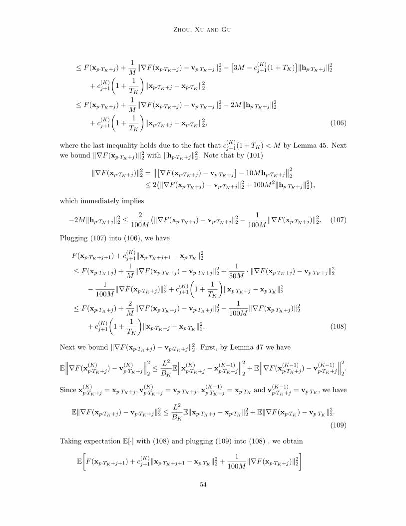
Zhou, Xu and Gu
≤ F (xp·TK+j) +1
M‖∇F (xp·TK+j)− vp·TK+j‖22 −
[3M − c(K)
j+1(1 + TK)]‖hp·TK+j‖22
+ c(K)j+1
(1 +
1
TK
)‖xp·TK+j − xp·TK‖22
≤ F (xp·TK+j) +1
M‖∇F (xp·TK+j)− vp·TK+j‖22 − 2M‖hp·TK+j‖22
+ c(K)j+1
(1 +
1
TK
)‖xp·TK+j − xp·TK‖22, (106)
where the last inequality holds due to the fact that c(K)j+1(1 + TK) < M by Lemma 45. Next
we bound ‖∇F (xp·TK+j)‖22 with ‖hp·TK+j‖22. Note that by (101)
‖∇F (xp·TK+j)‖22 =∥∥[∇F (xp·TK+j)− vp·TK+j
]− 10Mhp·TK+j
∥∥2
2
≤ 2(‖∇F (xp·TK+j)− vp·TK+j‖22 + 100M2‖hp·TK+j‖22
),
which immediately implies
−2M‖hp·TK+j‖22 ≤2
100M
(‖∇F (xp·TK+j)− vp·TK+j‖22 −
1
100M‖∇F (xp·TK+j)‖22. (107)
Plugging (107) into (106), we have
F (xp·TK+j+1) + c(K)j+1‖xp·TK+j+1 − xp·TK‖22
≤ F (xp·TK+j) +1
M‖∇F (xp·TK+j)− vp·TK+j‖22 +
1
50M· ‖∇F (xp·TK+j)− vp·TK+j‖22
− 1
100M‖∇F (xp·TK+j)‖22 + c
(K)j+1
(1 +
1
TK
)‖xp·TK+j − xp·TK‖22
≤ F (xp·TK+j) +2
M‖∇F (xp·TK+j)− vp·TK+j‖22 −
1
100M‖∇F (xp·TK+j)‖22
+ c(K)j+1
(1 +
1
TK
)‖xp·TK+j − xp·TK‖22. (108)
Next we bound ‖∇F (xp·TK+j)− vp·TK+j‖22. First, by Lemma 47 we have
E∥∥∥∇F (x
(K)p·TK+j)− v
(K)p·TK+j
∥∥∥2
2≤ L2
BKE∥∥∥x(K)
p·TK+j − x(K−1)p·TK+j
∥∥∥2
2+ E
∥∥∥∇F (x(K−1)p·TK+j)− v
(K−1)p·TK+j
∥∥∥2
2.
Since x(K)p·TK+j = xp·TK+j ,v
(K)p·TK+j = vp·TK+j , x
(K−1)p·TK+j = xp·TK and v
(K−1)p·TK+j = vp·TK , we have
E‖∇F (xp·TK+j)− vp·TK+j‖22 ≤L2
BKE‖xp·TK+j − xp·TK‖22 + E‖∇F (xp·TK )− vp·TK‖22.
(109)
Taking expectation E[·] with (108) and plugging (109) into (108) , we obtain
E[F (xp·TK+j+1) + c
(K)j+1‖xp·TK+j+1 − xp·TK‖22 +
1
100M‖∇F (xp·TK+j)‖22
]
54
Stochastic Nested Variance Reduction for Nonconvex Optimization
≤ E[F (xp·TK+j) +
(c
(K)j+1
(1 +
1
TK
)+
3L2
BKM
)‖xp·TK+j − xp·TK‖22
+2
M‖∇F (xp·TK )− vp·TK‖22
]
= E[F (xp·TK+j) + c
(K)j ‖xp·TK+j − xp·TK‖22 +
2
M· ‖∇F (xp·TK )− vp·TK‖22
], (110)
where (110) holds because we have c(K)j = c
(K)j+1(1 + 1/TK) + 3L2/(BKM) by Definition 41.
Telescoping (110) for j = 0 to end− start− 1, we have
E[F(xend
)+ c
(K)TK· ‖xend − xstart‖22
]+
1
100M
end−1∑
j=start
E‖∇F (xj)‖22
≤ E[F(xend
)+ c
(K)end−start · ‖xend − xstart‖22
]+
1
100M
end−1∑
j=start
E‖∇F (xj)‖22
≤ F (xstart) +2(end− start)
M· E‖∇F (xstart)− vstart‖22,
which completes the proof.
G.4. Proof of Lemma 47
Proof [Proof of Lemma 47] If tl = tl−1, we have x(l)t = x
(l−1)t and v
(l)t = v
(l−1)t . In this case
the statement in Lemma 47 holds trivially. Therefore, we assume tl 6= tl−1 in the followingproof. Note that
E[∥∥∇F (x
(l)t )− v
(l)t
∥∥2
2|Ftl
]
= E[∥∥∇F (x
(l)t )− v
(l)t − E
[∇F (x
(l)t )− v
(l)t
]∥∥2
2|Ftl
]+∥∥E[∇F (x
(l)t )− v
(l)t |Ftl
]∥∥2
2
= E
[∥∥∥∥∇F (x(l)t )−
l∑
j=0
g(j)t − E
[∇F (x
(l)t )−
l∑
j=0
g(j)t
]∥∥∥∥2
2
∣∣∣∣Ftl]
︸ ︷︷ ︸J1
+
∥∥∥∥E[∇F (x
(l)t )−
l∑
j=0
g(j)t
∣∣∣∣Ftl]∥∥∥∥
2
2︸ ︷︷ ︸
J2
,
(111)
where in the second equation we used the definition v(l)t =
∑li=0 g
(i)t in (72). We first upper
bound term J1. According to the update rule in Algorithm 1 (Line 20-23), when j < l, g(j)t
will not be updated at the tl-th iteration. Thus we have E[g(j)t |Ftl ] = g
(j)t for all j < l. In
addition, by the definition of Ftl , we have E[∇F (x(l)t )|Ftl ] = ∇F (x
(l)t ). Then we have the
following equation
J1 = E[∥∥g(l)
t − E[g
(l)t |Ftl
]∥∥2
2|Ftl
]. (112)
We further have
g(l)t =
1
Bl
∑
i∈I
[∇fi(x(l)
t )−∇fi(x(l−1)t )
], E
[g
(l)t
∣∣Ftl]
= ∇F (x(l)t )−∇F (x
(l−1)t ).
55
Zhou, Xu and Gu
Therefore, we can apply Lemma 43 to (112) and obtain
J1 ≤1
Bl· 1
n
n∑
i=1
∥∥∇fi(x(l)t )−∇fi(x(l−1)
t )−[∇F (x
(l)t )−∇F (x
(l−1)t )
]∥∥2
2
≤ 1
Bln
n∑
i=1
∥∥∇fi(x(l)t )−∇fi(x(l−1)
t )∥∥2
2
≤ L2
Bl
∥∥x(l)t − x
(l−1)t
∥∥2
2, (113)
where the second inequality is due to the fact that E[‖X − E[X]‖22] ≤ E‖X‖22 for anyrandom vector X and the last inequality holds due to the fact that F has averaged L-Lipschitz gradient.
Next we turn to bound term J2. Note that
E[g
(l)t
∣∣Ftl]
= E[
1
Bl
∑
i∈I
[∇fi(x(l)
t )−∇fi(x(l−1)t )
]∣∣∣∣Ftl]
= ∇F (x(l)t )−∇F (x
(l−1)t ),
which immediately implies
E[∇F (x
(l)t )−
l∑
j=0
g(j)t
∣∣∣∣Ftl]
= E[∇F (x
(l)t )−∇F (x
(l)t ) +∇F (x
(l−1)t )−
l−1∑
j=0
g(j)t
∣∣∣∣Ftl]
= E[∇F (x
(l−1)t )− v
(l−1)t
∣∣Ftl]
= ∇F (x(l−1)t )− v
(l−1)t ,
where the last equation is due to the definition of Ft. Plugging J1 and J2 into (111) yieldsthe following result:
E[∥∥∇F (x
(l)t )− v
(l)t
∥∥2
2
∣∣Ftl]≤ L2
Bl
∥∥x(l)t − x
(l−1)t
∥∥2
2+∥∥∇F (x
(l−1)t )− v
(l−1)t
∥∥2
2,
which completes the proof.
Appendix H. More Details of the Proposed Algorithms
In this section, we give additional details about the proposed algorithms. In particular,we will present an equivalent version of Algorithm 1, which shows an alternative view ofinterpreting it. We will also present the detailed Neon algorithm for the self-containedness.
H.1. An Equivalent Version of Algorithm 1
Recall the One-epoch-SNVRG algorithm in Algorithm 1. Here we present an equivalentversion of Algorithm 1 using nested loops, which is displayed in Algorithm 6 and is morealigned with the illustration in Figure 2(b). Note that the notation used in Algorithm 6 isslightly different from that in Algorithm 1 to avoid confusion.
56
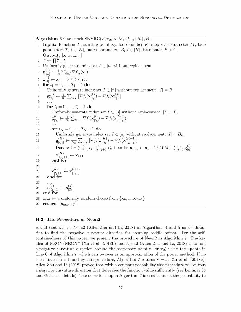
Stochastic Nested Variance Reduction for Nonconvex Optimization
Algorithm 6 One-epoch-SNVRG(F,x0,K,M, Ti, Bi, B)
1: Input: Function F , starting point x0, loop number K, step size parameter M , loopparameters Ti, i ∈ [K], batch parameters Bi, i ∈ [K], base batch B > 0.Output: [xout,xend]
2: T ←∏Kl=1 Tl
3: Uniformly generate index set I ⊂ [n] without replacement
4: g(0)[t0] ← 1
B
∑i∈I ∇fid(x0)
5: x(l)[0] ← x0, 0 ≤ l ≤ K,
6: for t1 = 0, . . . , T1 − 1 do7: Uniformly generate index set I ⊂ [n] without replacement, |I| = B1
8: g(1)[t1] ← 1
B1
∑i∈I[∇fi(x(1)
[t1])−∇fi(x(0)[0] )]
9: . . .10: for tl = 0, . . . , Tl − 1 do11: Uniformly generate index set I ⊂ [n] without replacement, |I| = Bl
12: g(l)[tl]← 1
Bl
∑i∈I[∇fi(x(l)
[tl])−∇fi(x(l−1)
[tl−1])]
13: . . .14: for tK = 0, . . . , TK − 1 do15: Uniformly generate index set I ⊂ [n] without replacement, |I| = BK
16: g(K)[tK ] ← 1
BK
∑i∈I[∇fi(x(K)
[tK ])−∇fi(x(K−1)[tK−1] )
]
17: Denote t =∑K
j=1 tj∏Kl=j+1 Tl, then let xt+1 ← xt − 1/(10M) ·∑K
l=0 g(l)[tl]
18: x(K)[tK+1] ← xt+1
19: end for20: . . .21: x
(l)[tl+1] ← x
(l+1)[Tl+1]
22: end for23: . . .24: x
(1)[t1+1] ← x
(2)[T2]
25: end for26: xout ← a uniformly random choice from x0, ...,xT−127: return [xout,xT ]
H.2. The Procedure of Neon2
Recall that we use Neon2 (Allen-Zhu and Li, 2018) in Algorithms 4 and 5 as a subrou-tine to find the negative curvature direction for escaping saddle points. For the self-containedness of this paper, we present the procedure of Neon2 in Algorithm 7. The keyidea of NEON/NEON+ (Xu et al., 2018b) and Neon2 (Allen-Zhu and Li, 2018) is to finda negative curvature direction around the stationary point z (or x0) using the update inLine 6 of Algorithm 7, which can be seen as an approximation of the power method. If nosuch direction is found by this procedure, Algorithm 7 returns v =⊥. Xu et al. (2018b);Allen-Zhu and Li (2018) proved that with a constant probability this procedure will outputa negative curvature direction that decreases the function value sufficiently (see Lemmas 33and 35 for the details). The outer for loop in Algorithm 7 is used to boost the probability to
57
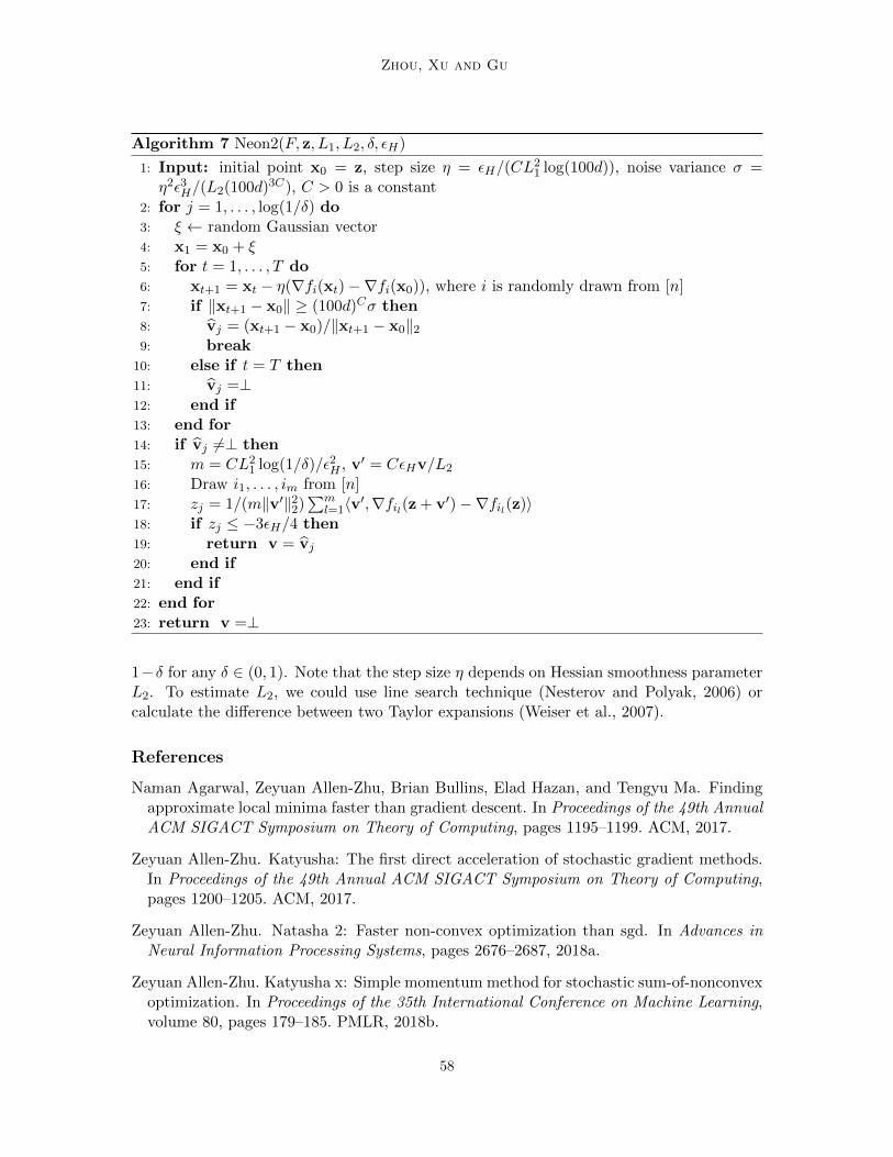
Zhou, Xu and Gu
Algorithm 7 Neon2(F, z, L1, L2, δ, εH)
1: Input: initial point x0 = z, step size η = εH/(CL21 log(100d)), noise variance σ =
η2ε3H/(L2(100d)3C), C > 0 is a constant2: for j = 1, . . . , log(1/δ) do3: ξ ← random Gaussian vector4: x1 = x0 + ξ5: for t = 1, . . . , T do6: xt+1 = xt − η(∇fi(xt)−∇fi(x0)), where i is randomly drawn from [n]7: if ‖xt+1 − x0‖ ≥ (100d)Cσ then8: vj = (xt+1 − x0)/‖xt+1 − x0‖29: break
10: else if t = T then11: vj =⊥12: end if13: end for14: if vj 6=⊥ then15: m = CL2
1 log(1/δ)/ε2H , v′ = CεHv/L2
16: Draw i1, . . . , im from [n]17: zj = 1/(m‖v′‖22)
∑ml=1〈v′,∇fil(z + v′)−∇fil(z)〉
18: if zj ≤ −3εH/4 then19: return v = vj20: end if21: end if22: end for23: return v =⊥
1−δ for any δ ∈ (0, 1). Note that the step size η depends on Hessian smoothness parameterL2. To estimate L2, we could use line search technique (Nesterov and Polyak, 2006) orcalculate the difference between two Taylor expansions (Weiser et al., 2007).
References
Naman Agarwal, Zeyuan Allen-Zhu, Brian Bullins, Elad Hazan, and Tengyu Ma. Findingapproximate local minima faster than gradient descent. In Proceedings of the 49th AnnualACM SIGACT Symposium on Theory of Computing, pages 1195–1199. ACM, 2017.
Zeyuan Allen-Zhu. Katyusha: The first direct acceleration of stochastic gradient methods.In Proceedings of the 49th Annual ACM SIGACT Symposium on Theory of Computing,pages 1200–1205. ACM, 2017.
Zeyuan Allen-Zhu. Natasha 2: Faster non-convex optimization than sgd. In Advances inNeural Information Processing Systems, pages 2676–2687, 2018a.
Zeyuan Allen-Zhu. Katyusha x: Simple momentum method for stochastic sum-of-nonconvexoptimization. In Proceedings of the 35th International Conference on Machine Learning,volume 80, pages 179–185. PMLR, 2018b.
58
Stochastic Nested Variance Reduction for Nonconvex Optimization
Zeyuan Allen-Zhu and Elad Hazan. Variance reduction for faster non-convex optimization.In International Conference on Machine Learning, pages 699–707, 2016.
Zeyuan Allen-Zhu and Yuanzhi Li. Neon2: Finding local minima via first-order oracles. InAdvances in Neural Information Processing Systems, pages 3720–3730, 2018.
Animashree Anandkumar and Rong Ge. Efficient approaches for escaping higher ordersaddle points in non-convex optimization. In Conference on Learning Theory, pages 81–102, 2016.
Srinadh Bhojanapalli, Behnam Neyshabur, and Nati Srebro. Global optimality of localsearch for low rank matrix recovery. In Advances in Neural Information Processing Sys-tems, pages 3873–3881, 2016.
Yair Carmon, John C Duchi, Oliver Hinder, and Aaron Sidford. “Convex until provenguilty”: Dimension-free acceleration of gradient descent on non-convex functions. InInternational Conference on Machine Learning, pages 654–663, 2017.
Yair Carmon, John C Duchi, Oliver Hinder, and Aaron Sidford. Accelerated methods fornonconvex optimization. SIAM Journal on Optimization, 28(2):1751–1772, 2018.
Xi Chen, Simon S Du, and Xin T Tong. On stationary-point hitting time and ergodicityof stochastic gradient langevin dynamics. Journal of Machine Learning Research, 21(68):1–41, 2020.
Anna Choromanska, Mikael Henaff, Michael Mathieu, Gerard Ben Arous, and Yann LeCun.The loss surfaces of multilayer networks. In Artificial Intelligence and Statistics, pages192–204, 2015.
Frank E Curtis, Daniel P Robinson, and Mohammadreza Samadi. A trust region algo-rithm with a worst-case iteration complexity of O(ε−3/2) for nonconvex optimization.Mathematical Programming, 162(1-2):1–32, 2017.
Hadi Daneshmand, Jonas Kohler, Aurelien Lucchi, and Thomas Hofmann. Escaping saddleswith stochastic gradients. In Proceedings of the 35th International Conference on MachineLearning, volume 80, pages 1155–1164. PMLR, 2018.
Yann Dauphin, Razvan Pascanu, Caglar Gulcehre, Kyunghyun Cho, Surya Ganguli, andYoshua Bengio. Identifying and attacking the saddle point problem in high-dimensionalnon-convex optimization. Mathematics, 111(6 Pt 1):2475–2485, 2014.
Aaron Defazio, Francis Bach, and Simon Lacoste-Julien. Saga: A fast incremental gradientmethod with support for non-strongly convex composite objectives. In Advances in NeuralInformation Processing Systems, pages 1646–1654, 2014a.
Aaron Defazio, Justin Domke, et al. Finito: A faster, permutable incremental gradientmethod for big data problems. In International Conference on Machine Learning, pages1125–1133, 2014b.
59
Zhou, Xu and Gu
Cong Fang, Chris Junchi Li, Zhouchen Lin, and Tong Zhang. Spider: Near-optimal non-convex optimization via stochastic path-integrated differential estimator. In Advances inNeural Information Processing Systems, pages 686–696, 2018.
Cong Fang, Zhouchen Lin, and Tong Zhang. Sharp analysis for nonconvex sgd escapingfrom saddle points. In Conference on Learning Theory, pages 1192–1234, 2019.
Dan Garber and Elad Hazan. Fast and simple pca via convex optimization. arXiv preprintarXiv:1509.05647, 2015.
Rong Ge, Furong Huang, Chi Jin, and Yang Yuan. Escaping from saddle pointsonlinestochastic gradient for tensor decomposition. In Conference on Learning Theory, pages797–842, 2015.
Rong Ge, Jason D Lee, and Tengyu Ma. Matrix completion has no spurious local minimum.In Advances in Neural Information Processing Systems, pages 2973–2981, 2016.
Saeed Ghadimi and Guanghui Lan. Stochastic first-and zeroth-order methods for nonconvexstochastic programming. SIAM Journal on Optimization, 23(4):2341–2368, 2013.
Saeed Ghadimi and Guanghui Lan. Accelerated gradient methods for nonconvex nonlinearand stochastic programming. Mathematical Programming, 156(1-2):59–99, 2016.
Saeed Ghadimi, Guanghui Lan, and Hongchao Zhang. Mini-batch stochastic approximationmethods for nonconvex stochastic composite optimization. Mathematical Programming,155(1-2):267–305, 2016.
Reza Harikandeh, Mohamed Osama Ahmed, Alim Virani, Mark Schmidt, Jakub Konecny,and Scott Sallinen. Stopwasting my gradients: Practical svrg. In Advances in NeuralInformation Processing Systems, pages 2251–2259, 2015.
Christopher J Hillar and Lek-Heng Lim. Most tensor problems are np-hard. Journal of theACM (JACM), 60(6):45, 2013.
Chi Jin, Rong Ge, Praneeth Netrapalli, Sham M Kakade, and Michael I Jordan. How toescape saddle points efficiently. In International Conference on Machine Learning, pages1724–1732, 2017.
Chi Jin, Praneeth Netrapalli, and Michael I. Jordan. Accelerated gradient descent escapessaddle points faster than gradient descent. In Proceedings of the 31st Conference OnLearning Theory, volume 75, pages 1042–1085. PMLR, 2018.
Rie Johnson and Tong Zhang. Accelerating stochastic gradient descent using predictivevariance reduction. In Advances in Neural Information Processing Systems, pages 315–323, 2013.
Hamed Karimi, Julie Nutini, and Mark Schmidt. Linear convergence of gradient andproximal-gradient methods under the polyak- lojasiewicz condition. In Joint EuropeanConference on Machine Learning and Knowledge Discovery in Databases, pages 795–811.Springer, 2016.
60
Stochastic Nested Variance Reduction for Nonconvex Optimization
Diederik P. Kingma and Jimmy Ba. Adam: A method for stochastic optimization. CoRR,abs/1412.6980, 2014.
Jonas Moritz Kohler and Aurelien Lucchi. Sub-sampled cubic regularization for non-convexoptimization. In Proceedings of the 34th International Conference on Machine Learning,volume 70, pages 1895–1904. PMLR, 2017.
Alex Krizhevsky. Learning multiple layers of features from tiny images. Technical report,Citeseer, 2009.
Yann LeCun, Leon Bottou, Yoshua Bengio, and Patrick Haffner. Gradient-based learningapplied to document recognition. Proceedings of the IEEE, 86(11):2278–2324, 1998.
Jason D Lee, Max Simchowitz, Michael I Jordan, and Benjamin Recht. Gradient descentonly converges to minimizers. In Conference on learning theory, pages 1246–1257, 2016.
Jason D Lee, Ioannis Panageas, Georgios Piliouras, Max Simchowitz, Michael I Jordan, andBenjamin Recht. First-order methods almost always avoid strict saddle points. Mathe-matical programming, 176(1-2):311–337, 2019.
Lihua Lei, Cheng Ju, Jianbo Chen, and Michael I Jordan. Non-convex finite-sum optimiza-tion via scsg methods. In Advances in Neural Information Processing Systems, pages2348–2358, 2017.
Kfir Y Levy. The power of normalization: Faster evasion of saddle points. arXiv preprintarXiv:1611.04831, 2016.
Hongzhou Lin, Julien Mairal, and Zaid Harchaoui. A universal catalyst for first-orderoptimization. In Advances in Neural Information Processing Systems, pages 3384–3392,2015.
Yurii Nesterov. Introductory lectures on convex optimization: A basic course, volume 87.Springer Science & Business Media, 2013.
Yurii Nesterov and Boris T Polyak. Cubic regularization of newton method and its globalperformance. Mathematical Programming, 108(1):177–205, 2006.
Yuval Netzer, Tao Wang, Adam Coates, Alessandro Bissacco, Bo Wu, and Andrew Y Ng.Reading digits in natural images with unsupervised feature learning. In NIPS workshopon deep learning and unsupervised feature learning, 2011.
Lam M Nguyen, Jie Liu, Katya Scheinberg, and Martin Takac. Sarah: A novel method formachine learning problems using stochastic recursive gradient. In Proceedings of the 34thInternational Conference on Machine Learning-Volume 70, pages 2613–2621. JMLR. org,2017a.
Lam M Nguyen, Jie Liu, Katya Scheinberg, and Martin Takac. Stochastic recursive gradientalgorithm for nonconvex optimization. arXiv preprint arXiv:1705.07261, 2017b.
61
Zhou, Xu and Gu
Lam M Nguyen, Marten van Dijk, Dzung T Phan, Phuong Ha Nguyen, Tsui-Wei Weng,and Jayant R Kalagnanam. Finite-sum smooth optimization with sarah. arXiv preprintarXiv:1901.07648, 2019.
Erkki Oja. Simplified neuron model as a principal component analyzer. Journal of mathe-matical biology, 15(3):267–273, 1982.
Boris Teodorovich Polyak. Gradient methods for minimizing functionals. Zhurnal Vychis-litel’noi Matematiki i Matematicheskoi Fiziki, 3(4):643–653, 1963.
Ning Qian. On the momentum term in gradient descent learning algorithms. Neural net-works, 12(1):145–151, 1999.
Maxim Raginsky, Alexander Rakhlin, and Matus Telgarsky. Non-convex learning viastochastic gradient langevin dynamics: a nonasymptotic analysis. In Conference onLearning Theory, pages 1674–1703, 2017.
Sashank Reddi, Manzil Zaheer, Suvrit Sra, Barnabas Poczos, Francis Bach, RuslanSalakhutdinov, and Alex Smola. A generic approach for escaping saddle points. InInternational Conference on Artificial Intelligence and Statistics, pages 1233–1242, 2018.
Sashank J Reddi, Ahmed Hefny, Suvrit Sra, Barnabas Poczos, and Alex Smola. Stochasticvariance reduction for nonconvex optimization. In International Conference on MachineLearning, pages 314–323, 2016a.
Sashank J Reddi, Suvrit Sra, Barnabas Poczos, and Alex Smola. Fast incremental methodfor smooth nonconvex optimization. In Decision and Control (CDC), 2016 IEEE 55thConference on, pages 1971–1977. IEEE, 2016b.
Herbert Robbins and Sutton Monro. A stochastic approximation method. The annals ofmathematical statistics, pages 400–407, 1951.
Nicolas L Roux, Mark Schmidt, and Francis R Bach. A stochastic gradient method with anexponential convergence rate for finite training sets. In Advances in Neural InformationProcessing Systems, pages 2663–2671, 2012.
Bernhard Scholkopf and Alexander J Smola. Learning with kernels: support vector ma-chines, regularization, optimization, and beyond. MIT press, 2002.
Shai Shalev-Shwartz. Sdca without duality, regularization, and individual convexity. InInternational Conference on Machine Learning, pages 747–754, 2016.
Shai Shalev-Shwartz and Tong Zhang. Stochastic dual coordinate ascent methods for regu-larized loss minimization. Journal of Machine Learning Research, 14(Feb):567–599, 2013.
Quoc Tran-Dinh, Nhan H Pham, Dzung T Phan, and Lam M Nguyen. A hybrid stochasticoptimization framework for stochastic composite nonconvex optimization. arXiv preprintarXiv:1907.03793, 2019.
Roman Vershynin. Introduction to the non-asymptotic analysis of random matrices. arXivpreprint arXiv:1011.3027, 2010.
62
Stochastic Nested Variance Reduction for Nonconvex Optimization
Zhe Wang, Kaiyi Ji, Yi Zhou, Yingbin Liang, and Vahid Tarokh. Spiderboost and momen-tum: Faster variance reduction algorithms. In Advances in Neural Information ProcessingSystems, pages 2403–2413, 2019.
Martin Weiser, Peter Deuflhard, and Bodo Erdmann. Affine conjugate adaptive newtonmethods for nonlinear elastomechanics. Optimisation Methods and Software, 22(3):413–431, 2007.
Lin Xiao and Tong Zhang. A proximal stochastic gradient method with progressive variancereduction. SIAM Journal on Optimization, 24(4):2057–2075, 2014.
Pan Xu, Jinghui Chen, Difan Zou, and Quanquan Gu. Global convergence of langevin dy-namics based algorithms for nonconvex optimization. In Advances in Neural InformationProcessing Systems, pages 3122–3133, 2018a.
Peng Xu, Fred Roosta, and Michael W Mahoney. Newton-type methods for non-convexoptimization under inexact hessian information. Mathematical Programming, pages 1–36,2019.
Yi Xu, Jing Rong, and Tianbao Yang. First-order stochastic algorithms for escaping fromsaddle points in almost linear time. In Advances in Neural Information Processing Sys-tems, pages 5531–5541, 2018b.
Yaodong Yu, Difan Zou, and Quanquan Gu. Saving gradient and negative curvature com-putations: Finding local minima more efficiently. arXiv preprint arXiv:1712.03950, 2017.
Yaodong Yu, Pan Xu, and Quanquan Gu. Third-order smoothness helps: Faster stochasticoptimization algorithms for finding local minima. In Advances in Neural InformationProcessing Systems, pages 4526–4536, 2018.
Xiao Zhang, Lingxiao Wang, Yaodong Yu, and Quanquan Gu. A primal-dual analysis ofglobal optimality in nonconvex low-rank matrix recovery. In International conference onmachine learning, 2018.
Yuchen Zhang, Percy Liang, and Moses Charikar. A hitting time analysis of stochasticgradient langevin dynamics. In Conference on Learning Theory, pages 1980–2022, 2017.
Dongruo Zhou and Quanquan Gu. Lower bounds for smooth nonconvex finite-sum opti-mization. In International Conference on Machine Learning, pages 7574–7583, 2019.
Dongruo Zhou, Pan Xu, and Quanquan Gu. Stochastic variance-reduced cubic regular-ized Newton methods. In Proceedings of the 35th International Conference on MachineLearning, pages 5990–5999. PMLR, 2018a.
Dongruo Zhou, Pan Xu, and Quanquan Gu. Stochastic nested variance reduced gradi-ent descent for nonconvex optimization. In Advances in Neural Information ProcessingSystems, pages 3922–3933, 2018b.
63


![[Poster Presentation] Nonconvex Optimization …rhayakawa/paper/RCC2019...[Poster Presentation] Nonconvex Optimization Based Algorithm for Discrete-Valued Vector Reconstruction Ryo](https://img.pdfslide.net/doc/110x75/5f0609c97e708231d415fbb0/poster-presentation-nonconvex-optimization-rhayakawapaperrcc2019-poster.jpg)