Stochastic prediction of hourly global solar radiation profiles

S. Kaplanis, E. KaplaniMech. Engineering department, T.E.I. of Patra, Meg.

Alexandrou 1, Patrakaplanis@teipat.gr

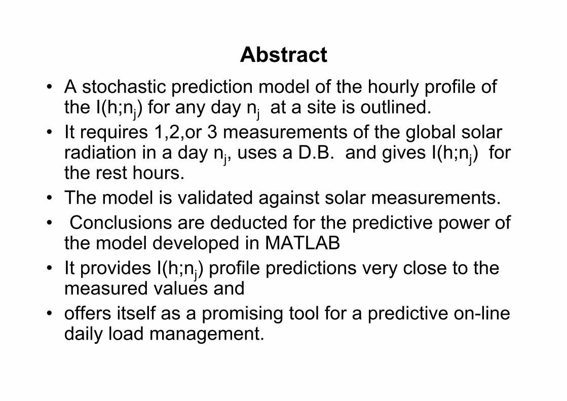
Abstract• A stochastic prediction model of the hourly profile of

the I(h;nj) for any day nj at a site is outlined. • It requires 1,2,or 3 measurements of the global solar

radiation in a day nj, uses a D.B. and gives I(h;nj) for the rest hours.

• The model is validated against solar measurements.• Conclusions are deducted for the predictive power of

the model developed in MATLAB • It provides I(h;nj) profile predictions very close to the

measured values and • offers itself as a promising tool for a predictive on-line

daily load management.

Introduction• The prediction of the global solar radiation

I(h;nj) on an hourly, h, basis, for any day, nj, was the target of many attempts internationally.

• Review papers outline and compare the meanexpected, Im,exp(h;nj), values which are the results of several such significant approaches.

• A reliable methodology to predict the I(h;nj) profile, based on few data, taking into account morning measurement(s) and simulating the statistics of I(h;nj), is a challenge.

• A model to predict close to reality I(h;nj) values would be useful in problems such as:

1. Meteo purposes2. Sizing effectively and reliably the solar power systems

i.e. PV generators 3. Management of solar energy sources, i.e. the output

of the PV systems, as affected by the meteo conditions in relation to the power loads to be met .

• The above issues drive the research activities towards the development of an improved effective methodology to predict the I(h;nj) for any day, nj, of the year at any site with latitude φ.

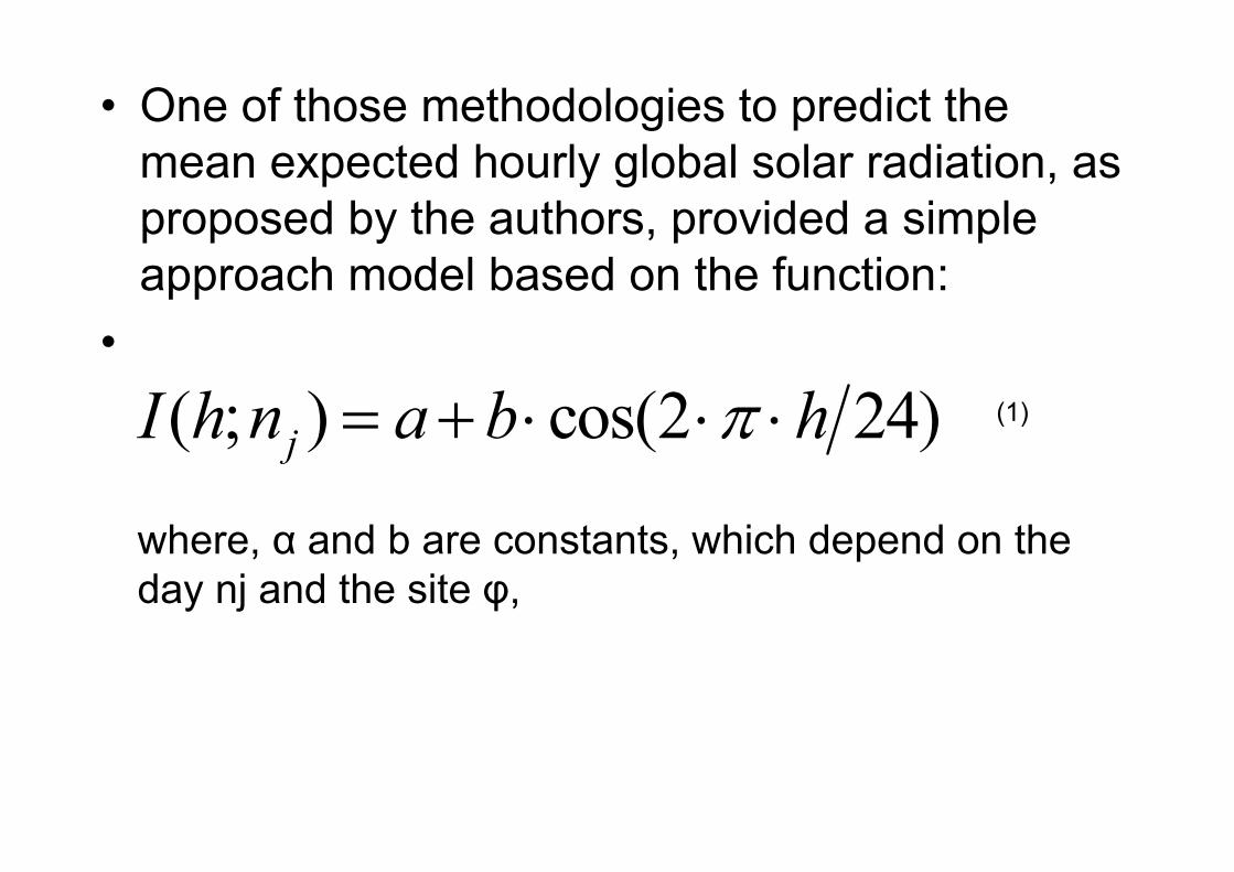
• One of those methodologies to predict the mean expected hourly global solar radiation, as proposed by the authors, provided a simple approach model based on the function:

•(1)( ; ) cos(2 24)jI h n a b h

where, α and b are constants, which depend on the day nj and the site φ,

• This model, overestimates I(h;nj) at the early morning and late afternoon hours, while it underestimates I(h;nj) around the solar noon hours.

• Although, the Ipr(h;nj) values fall, in general, within the range of the measured Imes(h;nj) fluctuations, a more accurate and dynamic model had to be developed.

• That model should have inbuilt statistical fluctuations, like the METEONORM package, but with a more effective prediction power.

• A comparison of the Ipr(h;nj) values between METEONORM and the generalised model versions, outlined, in contrast to measured Imes(h;nj) values, during the years (1995-2000), will be highlighted.

Basic Theoretical Analysis

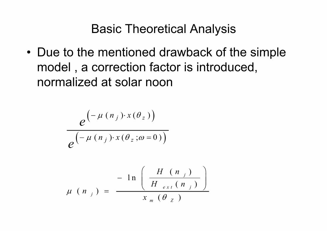
• Due to the mentioned drawback of the simple model , a correction factor is introduced, normalized at solar noon

( ) ( )

( ) ( ; 0 )

j z

j z

n x

n x

e

e

( )l n

( )( )

( )

j

e x t jj

m Z

H nH n

nx

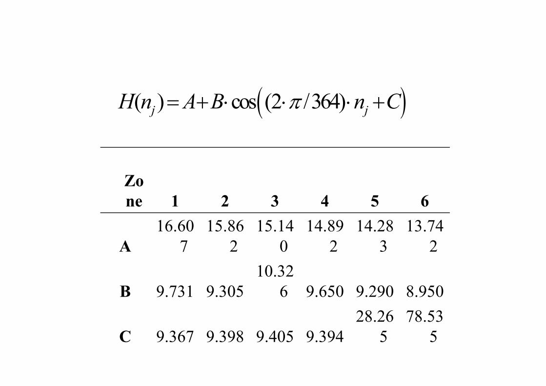
( ) cos (2 /364)j jH n A B n C

Zone 1 2 3 4 5 6

A16.60

715.86

215.14

014.89

214.28

313.74

2

B 9.731 9.30510.32

6 9.650 9.290 8.950

C 9.367 9.398 9.405 9.39428.26

578.53

5

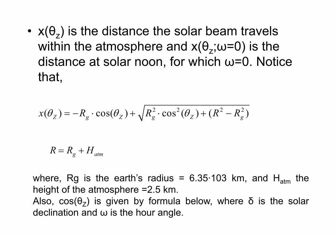
• x(θz) is the distance the solar beam travels within the atmosphere and x(θz;ω=0) is the distance at solar noon, for which ω=0. Notice that,

2 2 2 2( ) cos( ) cos ( ) ( )Z g Z g Z gx R R R R

g atmR R H

where, Rg is the earth’s radius = 6.35·103 km, and Hatm theheight of the atmosphere =2.5 km.Also, cos(θZ) is given by formula below, where δ is the solardeclination and ω is the hour angle.

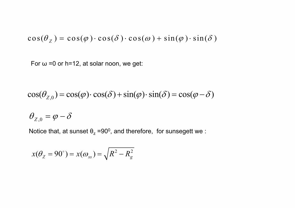
cos( ) cos( ) cos( ) cos( ) s in ( ) s in ( )Z

For ω =0 or h=12, at solar noon, we get:

,0cos( ) cos( ) cos( ) sin( ) sin( ) cos( )Z

,0Z

Notice that, at sunset θz =900, and therefore, for sunsegett we :

2 2( 90 ) ( )Z ss gx x R R

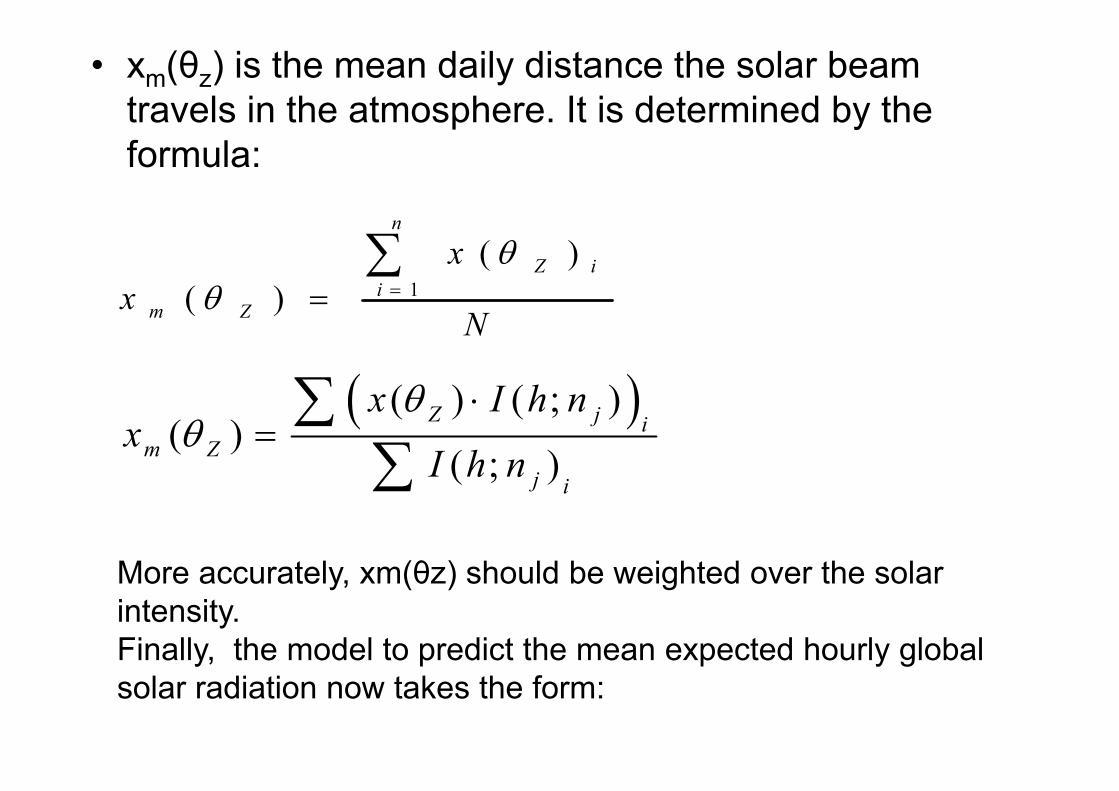
• xm(θz) is the mean daily distance the solar beam travels in the atmosphere. It is determined by the formula:

1( )

( )

n

Z ii

m Z

xx

N

( ) ( ; )( )

( ; )Z j i

m Zj i

x I h nx

I h n

More accurately, xm(θz) should be weighted over the solar intensity.Finally, the model to predict the mean expected hourly global solar radiation now takes the form:

( ) ( )

( ) ( 1 2 )

c o s 2 2 4( ; )

j

j

n x h

j n x h

e hI h n b

e

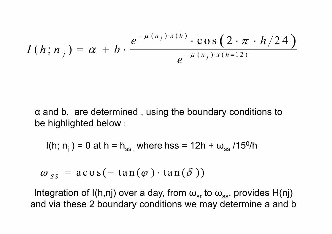
α and b, are determined , using the boundary conditions to be highlighted below :

I(h; nj ) = 0 at h = hss , where hss = 12h + ωss /150/h

a c o s ( ta n ( ) ta n ( ) )S S

Integration of I(h,nj) over a day, from ωsr to ωss, provides H(nj) and via these 2 boundary conditions we may determine a and b

0100200300400500600700800900

0 2 4 6 8 10 12 14 16 18 20 22 24

hour

Sola

r R

adia

tion

(Wh/

m^2 1995

19961997199819992000Predicted

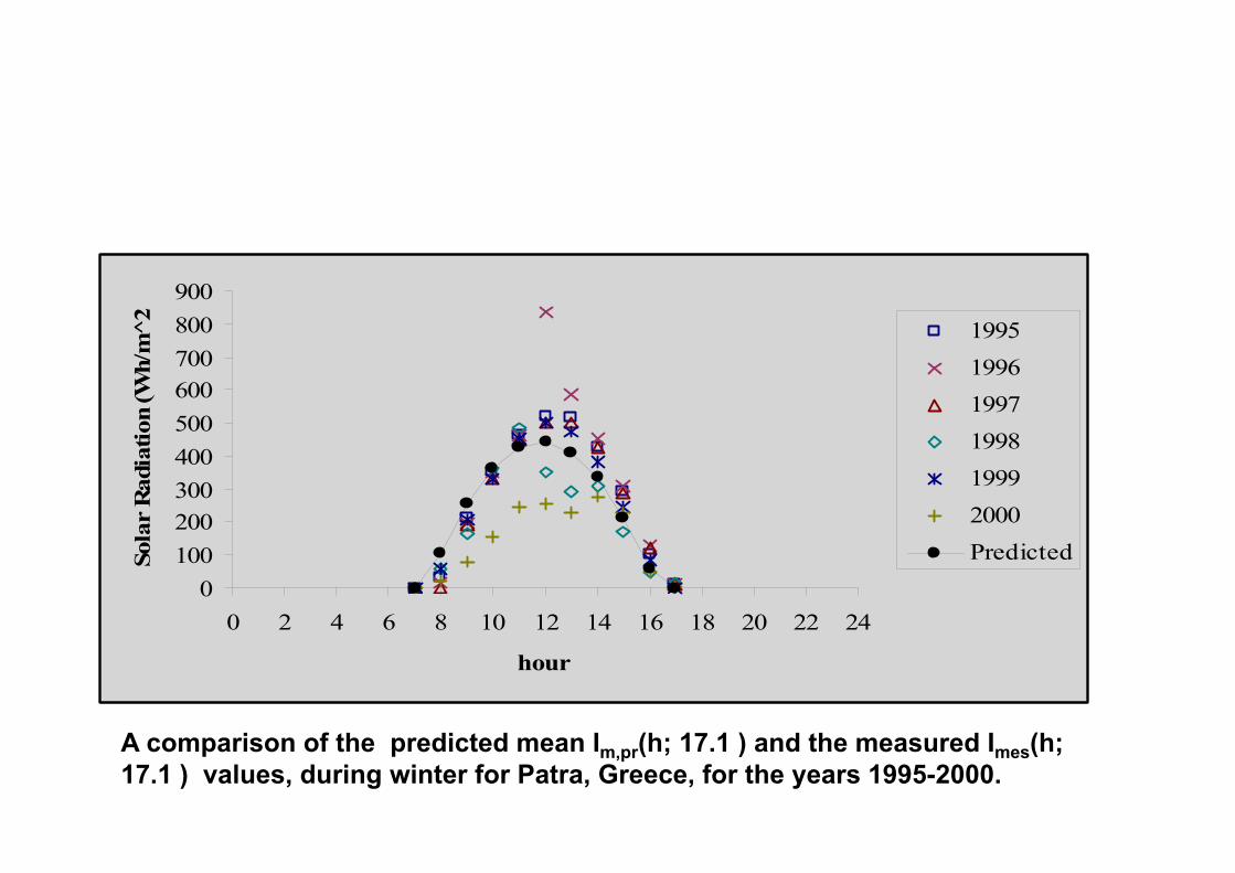
A comparison of the predicted mean Im,pr(h; 17.1 ) and the measured Imes(h; 17.1 ) values, during winter for Patra, Greece, for the years 1995-2000.

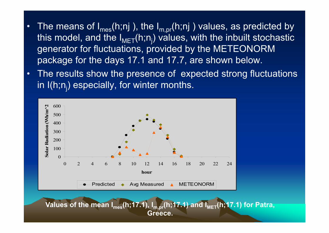
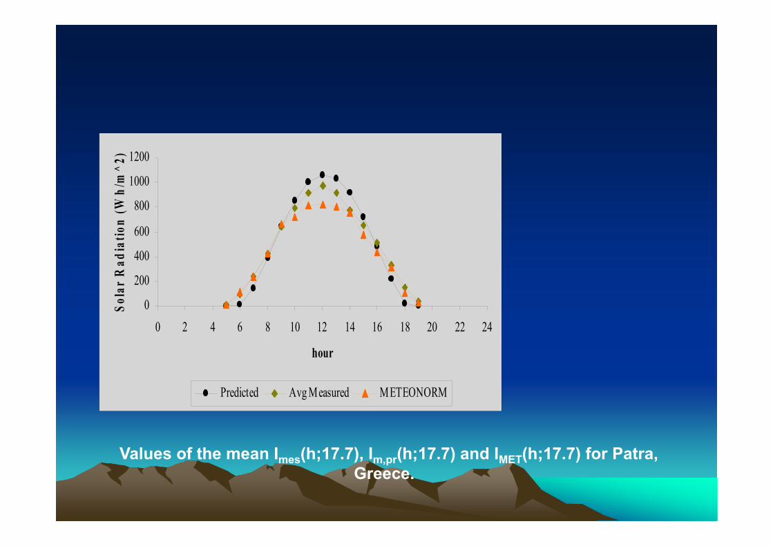
• The means of Imes(h;nj ), the Im,pr(h;nj ) values, as predicted by this model, and the IMET(h;nj) values, with the inbuilt stochastic generator for fluctuations, provided by the METEONORM package for the days 17.1 and 17.7, are shown below.

• The results show the presence of expected strong fluctuations in I(h;nj) especially, for winter months.

0

100

200

300

400

500

600

0 2 4 6 8 10 12 14 16 18 20 22 24

hour

Sola

r R

adia

tion

(Wh/

m^2

Predicted Avg Measured METEONORM

Values of the mean Imes(h;17.1), Im,pr(h;17.1) and IMET(h;17.1) for Patra,Greece.

0

200

400

600

800

1000

1200

0 2 4 6 8 10 12 14 16 18 20 22 24

hour

Sola

r R

adia

tion

(Wh/

m^2

)

Predicted Avg Measured METEONORM

Values of the mean Imes(h;17.7), Im,pr(h;17.7) and IMET(h;17.7) for Patra,Greece.

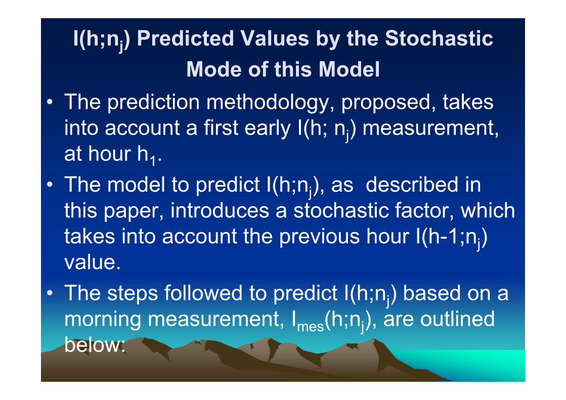
I(h;nj) Predicted Values by the Stochastic Mode of this Model

• The prediction methodology, proposed, takes into account a first early I(h; nj) measurement, at hour h1.

• The model to predict I(h;nj), as described in this paper, introduces a stochastic factor, which takes into account the previous hour I(h-1;nj) value.

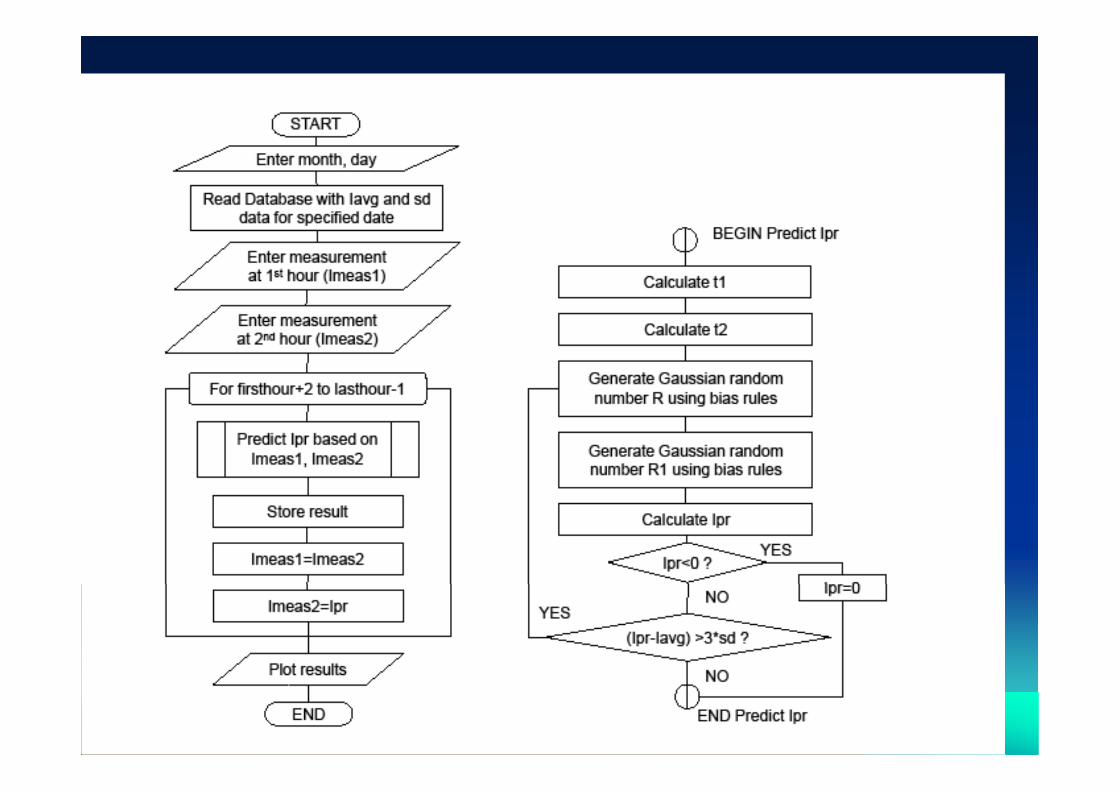
• The steps followed to predict I(h;nj) based on a morning measurement, Imes(h;nj), are outlined below:

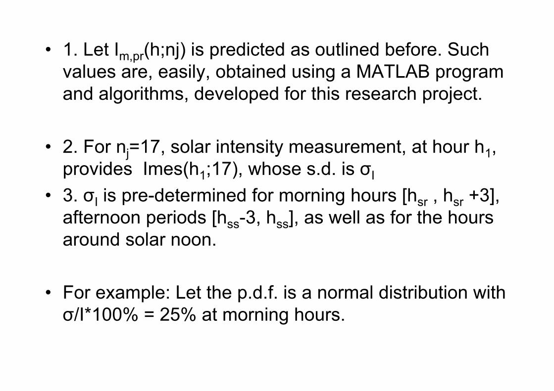
• 1. Let Im,pr(h;nj) is predicted as outlined before. Such values are, easily, obtained using a MATLAB program and algorithms, developed for this research project.

• 2. For nj=17, solar intensity measurement, at hour h1, provides Imes(h1;17), whose s.d. is σΙ

• 3. σΙ is pre-determined for morning hours [hsr , hsr +3], afternoon periods [hss-3, hss], as well as for the hours around solar noon.

• For example: Let the p.d.f. is a normal distribution with σ/Ι*100% = 25% at morning hours.

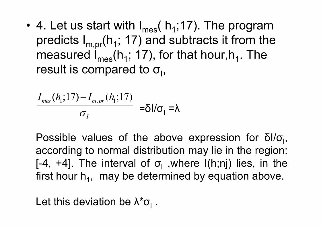
• 4. Let us start with Imes( h1;17). The program predicts Im,pr(h1; 17) and subtracts it from the measured Imes(h1; 17), for that hour,h1. The result is compared to σI,

1 , 1( ;17) ( ;17)mes m pr

I

I h I h

=δΙ/σΙ =λ

Possible values of the above expression for δI/σΙ,according to normal distribution may lie in the region:[-4, +4]. The interval of σI ,where I(h;nj) lies, in thefirst hour h1, may be determined by equation above.

Let this deviation be λ*σΙ .

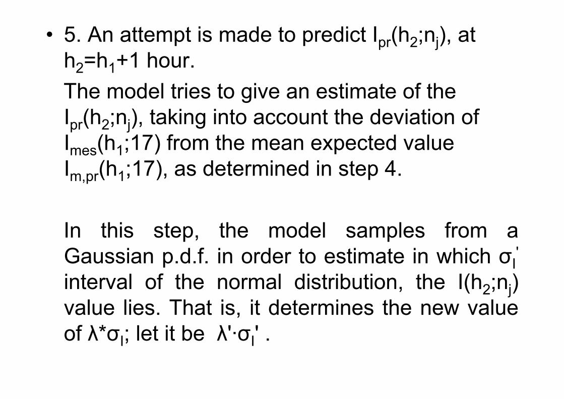
• 5. An attempt is made to predict Ιpr(h2;nj), at h2=h1+1 hour. The model tries to give an estimate of the Ιpr(h2;nj), taking into account the deviation of Imes(h1;17) from the mean expected value Im,pr(h1;17), as determined in step 4.

In this step, the model samples from aGaussian p.d.f. in order to estimate in which σI

'

interval of the normal distribution, the I(h2;nj)value lies. That is, it determines the new valueof λ*σΙ; let it be λ'·σI' .

• 6.The predicted value of I(h2;nj) is given, in this step, based on the mean expected Im,pr(h2;17), with a new deviation value λ'·σI', i.e.

Ipr(h2;nj)= Im,pr(h2;nj) ± λ'·σI'

λ' is determined through a Gaussian sampling and is permitted to take, according to this model, values within

the range λ±1.7. The model, then, determines the Ipr(h2;nj) value and

compares it with the mean expected Im,pr(h2;nj). It repeats the cycle, steps 4-6, for the h3 hour and so on.

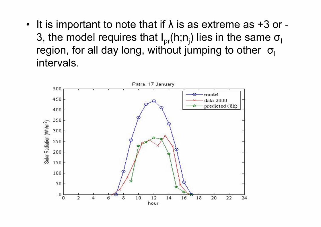
• It is important to note that if λ is as extreme as +3 or -3, the model requires that Ipr(h;nj) lies in the same σIregion, for all day long, without jumping to other σIintervals.

From Mode I: I(h;nj) prediction based on one morning

measurement to Mode II: I(h;nj) prediction based on two

morning measurements• Mode II of this model considers for the I(h;nj)

prediction two morning solar radiation measurements.

• In addition to Mode I, it takes into account the rate of change of the difference [Imeas(h;nj)- Iav(h;nj)], during the period from h1 to h2.

• Conclusively, it includes two stochastic terms, one term which stands for the stochastic fluctuations at hour h3, and

• a second term to stand for the rate of change of the I(h;nj), within the time interval [h1, h2].

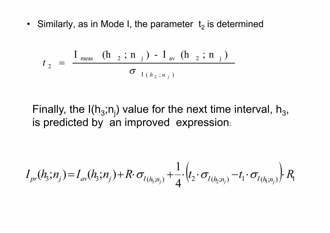
• Similarly, as in Mode I, the parameter t2 is determined

);(I

j2avj2meas2

2

)n;(hI -)n;(hI

jnh

t

Finally, the I(h3;nj) value for the next time interval, h3,is predicted by an improved expression:

1);(1);(2);(33 123 41);();( RttRnhInhI

jjj nhInhInhIjavjpr

• σI(h2;nj) and σI(h3;nj) are the s.d. of the measured I(h;nj) values at hours h2 and h3, respectively, in the day nj, as obtained from the D.B.

• Furthermore, the model proceeds to predict the Ipr(h4;nj) value. This is based on Ipr(h3;nj), which is the previous hour, h3, predicted value and the measured Imeas(h2;nj) one.

• Further on, it may predict Ipr(h5;nj), based on the previously predicted values Ipr(h3;nj) and Ipr(h4;nj), and so on.

• Notice that, R is a random number which may take values within t2± 1.

• This implies that from hour to hour, one may not expect weather variations larger than ±1*σI

• R1 is randomly distributed according to a Gaussian p.d.f. (0, 1). The term (t2*σI(h2;nj) - t1*σI(h1;nj))*R1stands for the contribution to the I(h;nj) prediction by its rate of change during the 2 previous hours.

This contribution is estimated by the relative positions of the measured Imeas(h1;nj) and Imeas(h2;nj), with reference to the average values Iav(h1;nj) and Iav(h2;nj), one by one.

• The above Formula expresses the superposition principle of two processes.

• The first one is the short term stochastic behaviour which provides expected hourly fluctuations based on the past history of the stored data for the hour h of a day nj.

• The second one represents the present trend of the hourly I(h;nj) measurements during the interval h1 to h2. This trend is weighted over a Gaussian p.d.f., (0, 1), which underlines that the two processes, short and long term, are independent to each other, and this ensemble represents the real phenomenon.

Mode III: I(h;nj) prediction based on three morning measurements

• The Mode III of the proposed model takes into consideration 3 morning solar global radiation measurements for the prediction of I(h;nj).

• According to the concept presented earlier, the prediction of I(h4;nj) at hour h4 is based on the following formula, which is more advanced than the previous two.

22

91

141);();(

);(1);(2);(3

);(2);(3);(44

123

234

Rttt

RttRnhInhI

jjj

jjj

nhInhInhI

nhInhInhIjavjpr

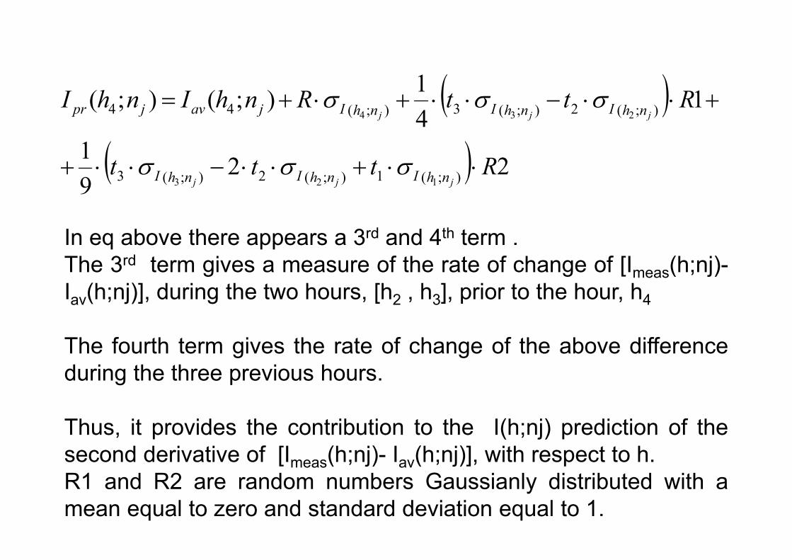
In eq above there appears a 3rd and 4th term .The 3rd term gives a measure of the rate of change of [Imeas(h;nj)-Iav(h;nj)], during the two hours, [h2 , h3], prior to the hour, h4

The fourth term gives the rate of change of the above differenceduring the three previous hours.

Thus, it provides the contribution to the I(h;nj) prediction of thesecond derivative of [Imeas(h;nj)- Iav(h;nj)], with respect to h.R1 and R2 are random numbers Gaussianly distributed with amean equal to zero and standard deviation equal to 1.

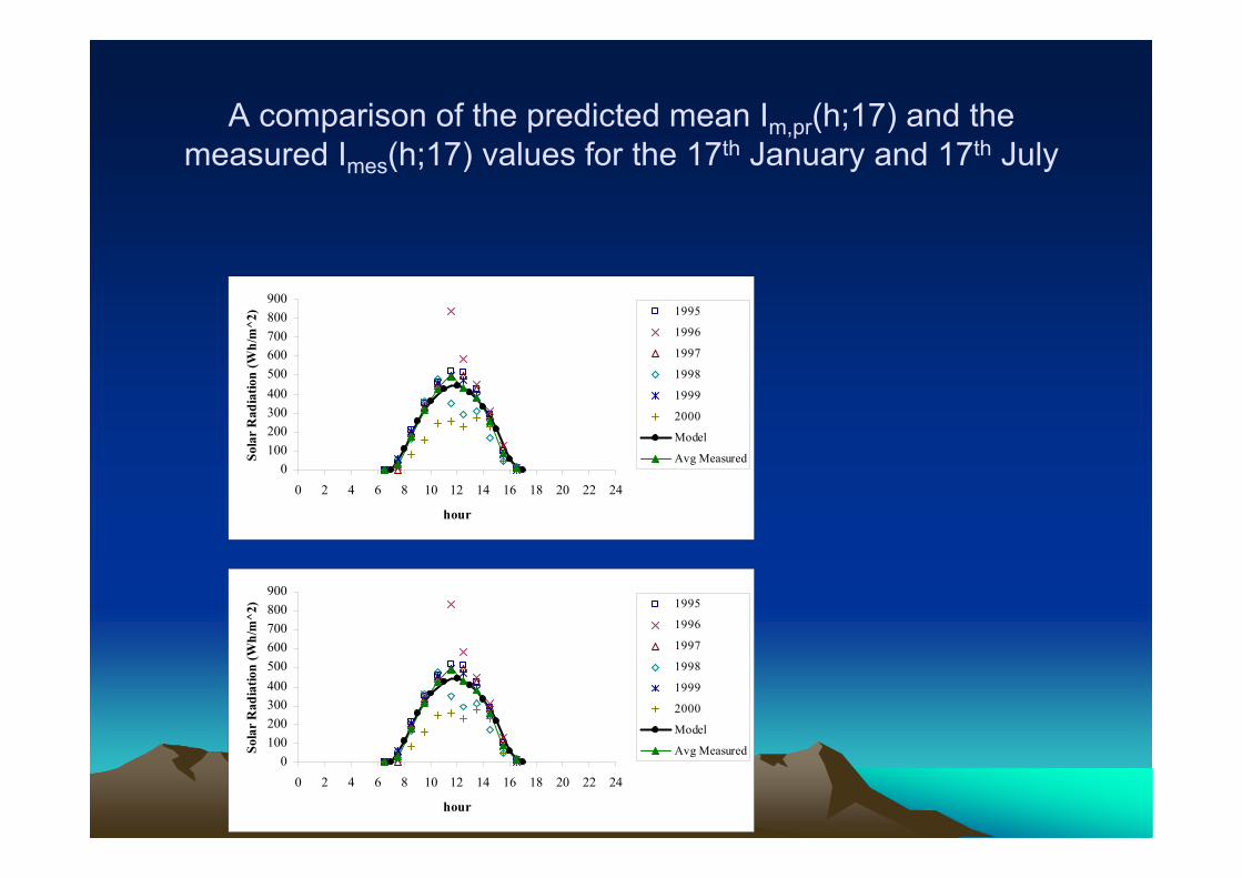
A comparison of the predicted mean Im,pr(h;17) and the measured Imes(h;17) values for the 17th January and 17th July

0100200300400500600700800900

0 2 4 6 8 10 12 14 16 18 20 22 24

hour

Sola

r R

adia

tion

(Wh/

m^2

) 1995

1996

1997

1998

1999

2000

Model

Avg Measured

0100200300400500600700800900

0 2 4 6 8 10 12 14 16 18 20 22 24

hour

Sola

r R

adia

tion

(Wh/

m^2

) 1995

1996

1997

1998

1999

2000

Model

Avg Measured

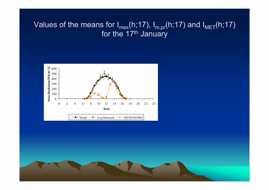
Values of the means for Imes(h;17), Im,pr(h;17) and IMET(h;17) for the 17th January

0100200300400500600

0 2 4 6 8 10 12 14 16 18 20 22 24

Sola

r Rad

iatio

n (W

h/m

^2)

hour

Model Avg Measured METEONORM

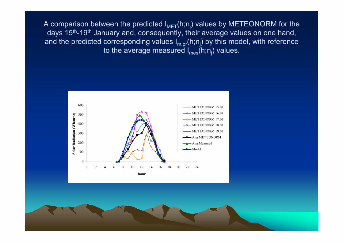
A comparison between the predicted IMET(h;nj) values by METEONORM for the days 15th-19th January and, consequently, their average values on one hand, and the predicted corresponding values

Im,pr(h;nj) by this model, with reference to the average measured Imes(h;nj) values.

0

100

200

300

400

500

600

0 2 4 6 8 10 12 14 16 18 20 22 24

hour

Sola

r R

adia

tion

(Wh/

m^2

)

METEONORM 15.01

METEONORM 16.01

METEONORM 17.01

METEONORM 18.01

METEONORM 19.01

Avg METEONORM

Avg Measured

Model

A comparison between the predicted IMET(h;nj) values by METEONORM for the days 15th-19th January and, consequently, their average values on one hand,

and the predicted corresponding values Im,pr(h;nj) by this model, with reference to the average measured Imes(h;nj) values.

0

100

200

300

400

500

600

0 2 4 6 8 10 12 14 16 18 20 22 24

hour

Sola

r R

adia

tion

(Wh/

m^2

)

METEONORM 15.01

METEONORM 16.01

METEONORM 17.01

METEONORM 18.01

METEONORM 19.01

Avg METEONORM

Avg Measured

Model

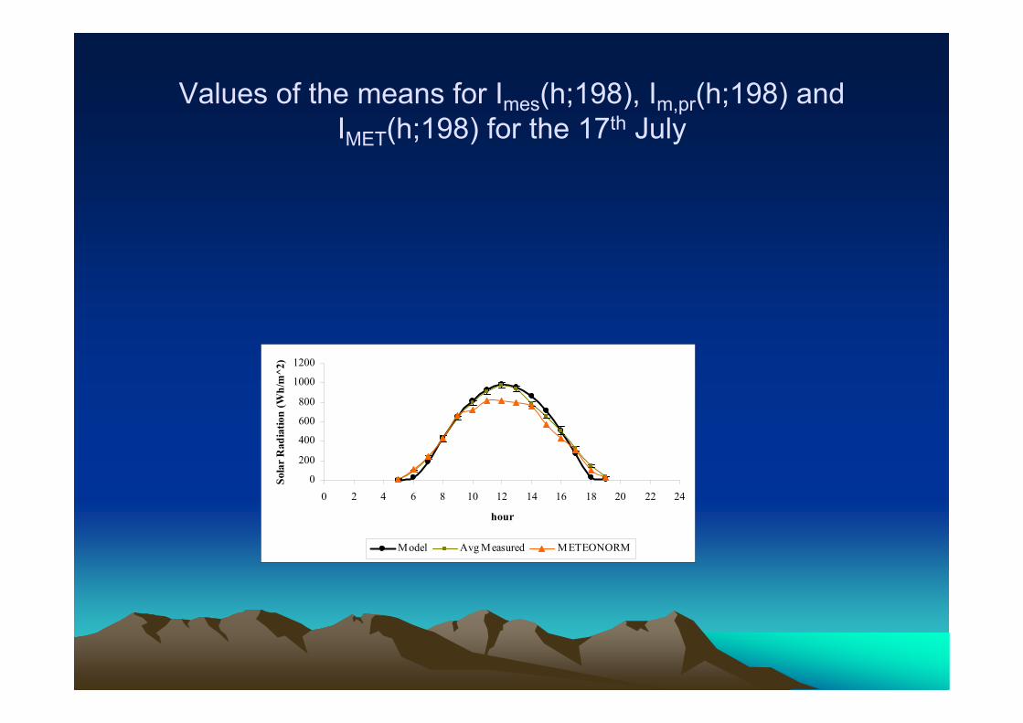
Values of the means for Imes(h;198), Im,pr(h;198) and IMET(h;198) for the 17th July

0

200

400

600

800

1000

1200

0 2 4 6 8 10 12 14 16 18 20 22 24

hour

Sola

r R

adia

tion

(Wh/

m^2

)

Model Avg Measured METEONORM

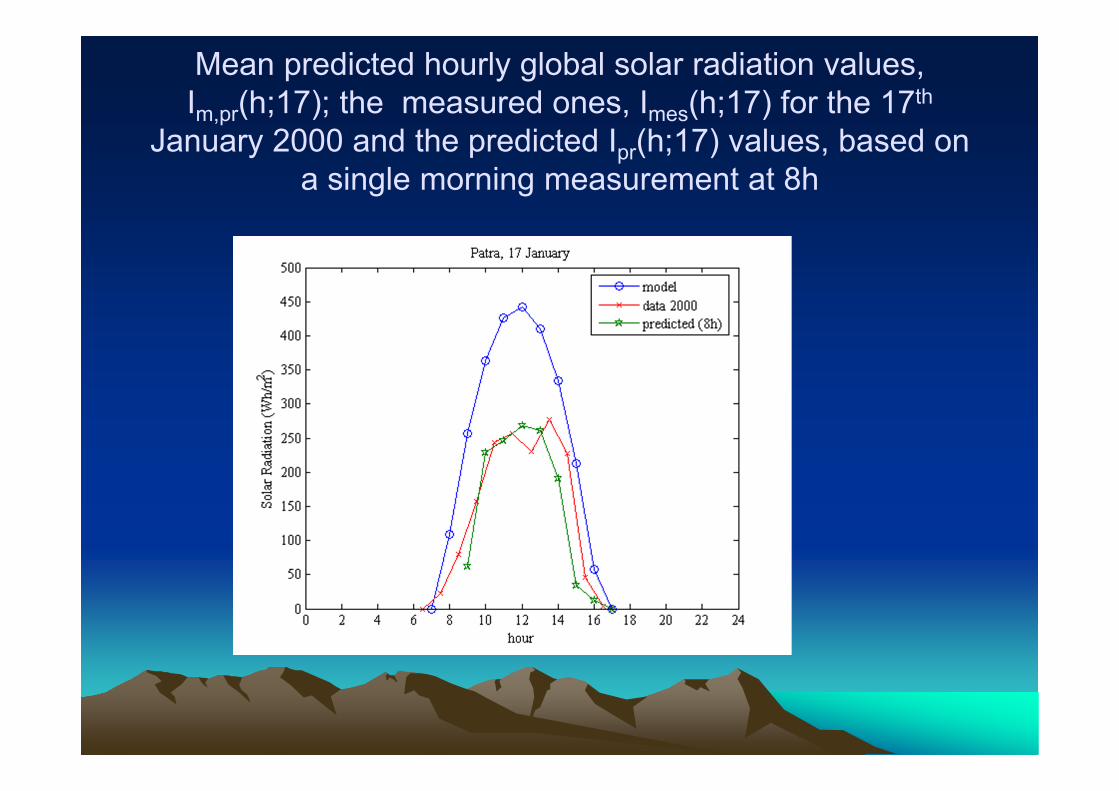
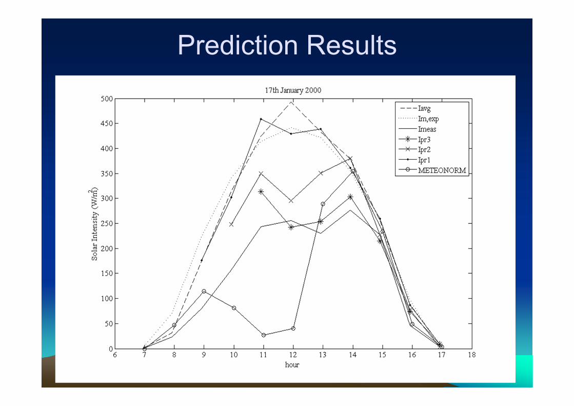
Mean predicted hourly global solar radiation values, Im,pr(h;17); the measured ones, Imes(h;17) for the 17th

January 2000 and the predicted Ipr(h;17) values, based on a single morning measurement at 8h

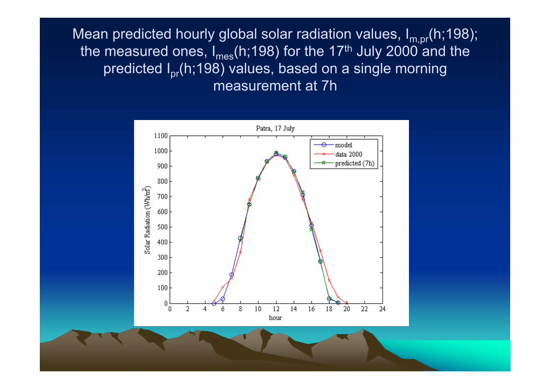
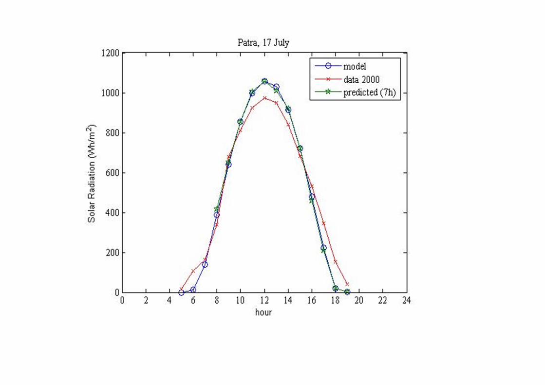
Mean predicted hourly global solar radiation values, Im,pr(h;198); the measured ones, Imes(h;198) for the 17th July 2000 and the

predicted Ipr(h;198) values, based on a single morning measurement at 7h

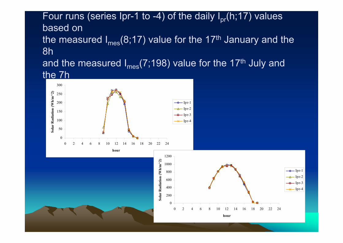
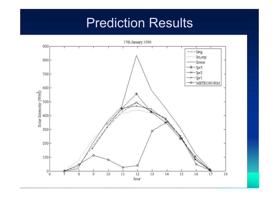
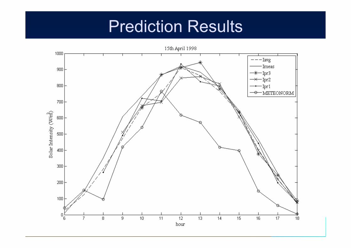
Four runs (series Ipr-1 to -4) of the daily Ipr(h;17) values based on the measured Imes(8;17) value for the 17th January and the 8h and the measured Imes(7;198) value for the 17th July and the 7h

0

50

100

150

200

250

300

0 2 4 6 8 10 12 14 16 18 20 22 24

hour

Sola

r R

adia

tion

(Wh/

m^2

)

Ipr-1

Ipr-2

Ipr-3

Ipr-4

0

200

400

600

800

1000

1200

0 2 4 6 8 10 12 14 16 18 20 22 24

hour

Sola

r R

adia

tion

(Wh/

m^2

)

Ipr-1

Ipr-2

Ipr-3

Ipr-4

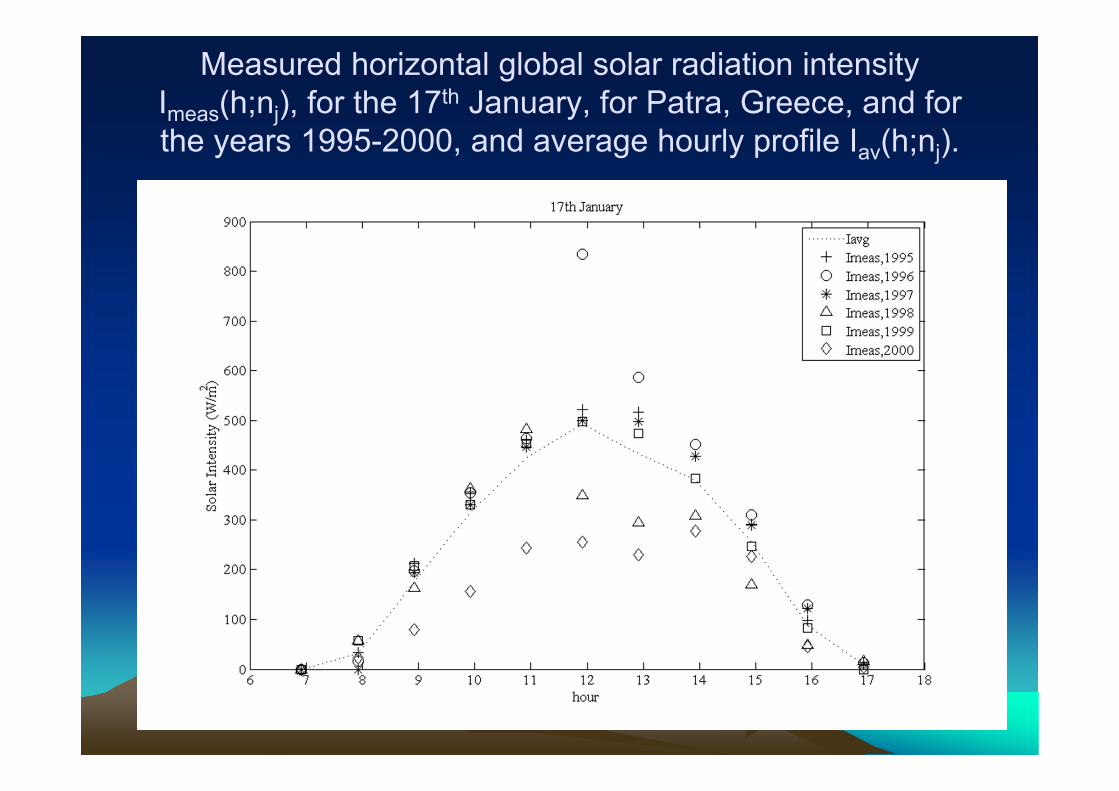
Measured horizontal global solar radiation intensity Imeas(h;nj), for the 17th January, for Patra, Greece, and for the years 1995-2000, and average hourly profile Iav(h;nj).

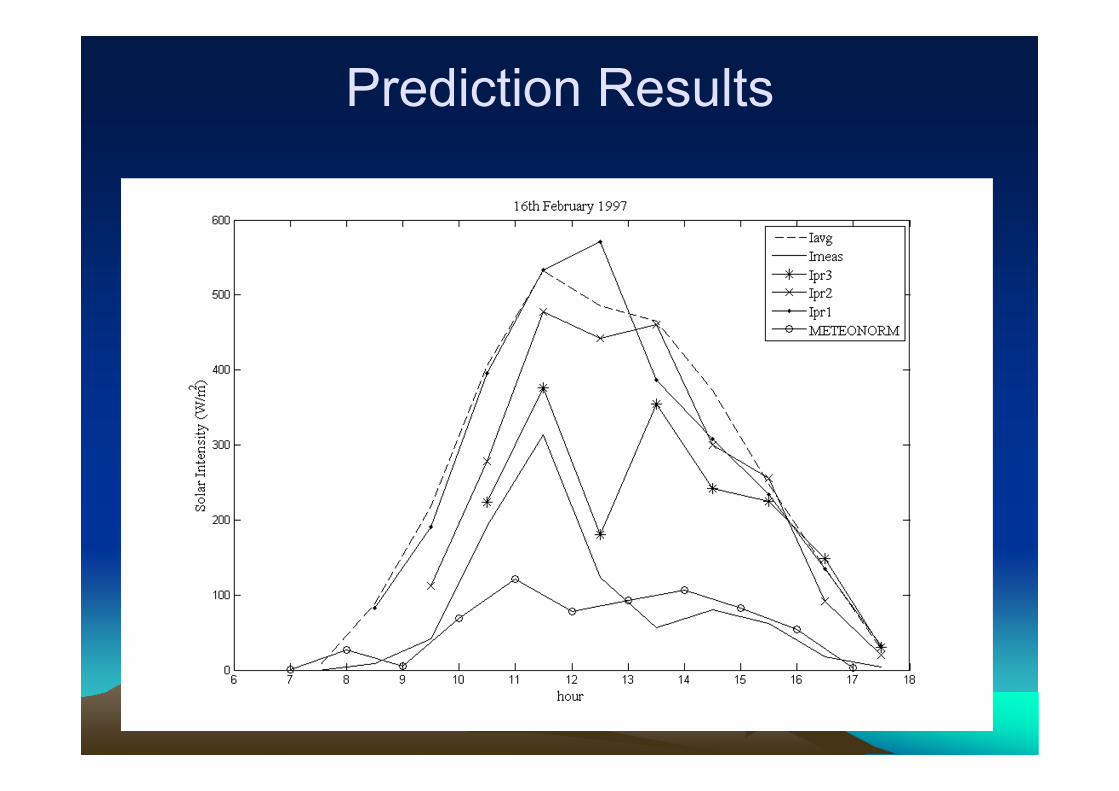
Prediction Results

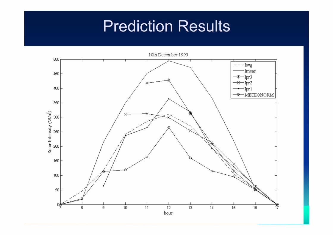
Prediction Results

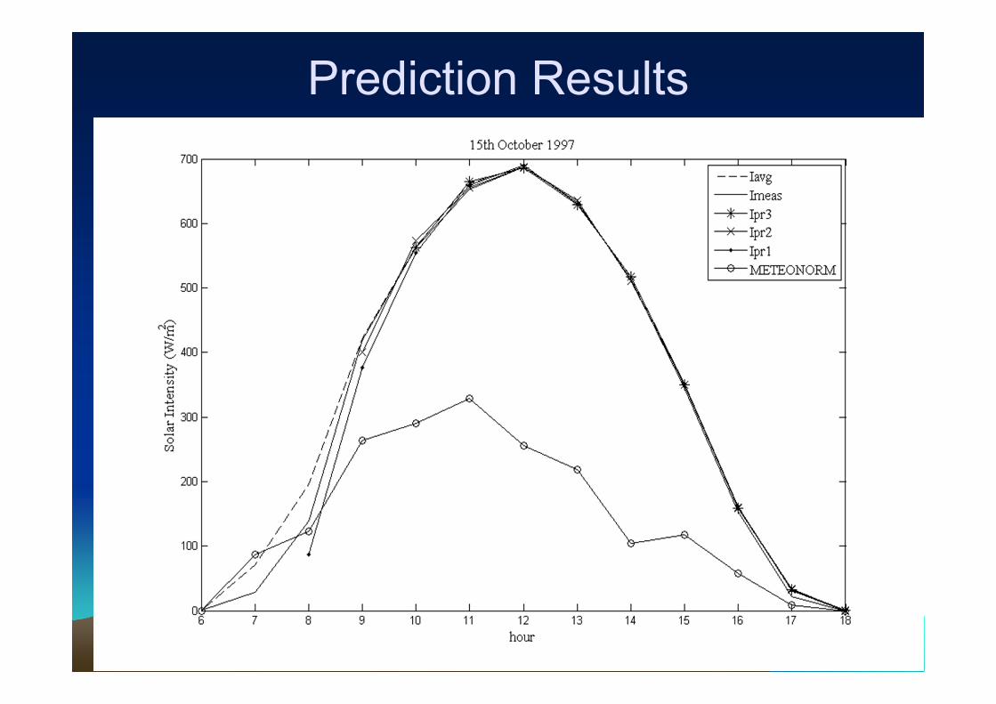
Prediction Results

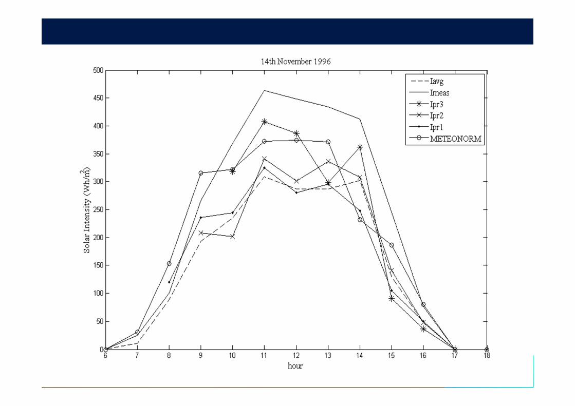
Prediction Results

Prediction Results

Prediction Results

Prediction Results

Prediction Results

Prediction Results

Discussion• The model outlined is based on the assumption that

the relative position of Imeas(h;nj) with respect to Im,exp(h;nj) or with respect to Iav(h;nj) may not change more than ±1*σI per hour, for mild climates.

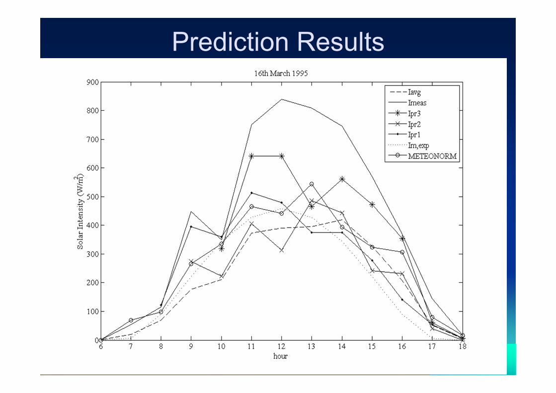
• Generally, Mode I provides good estimates of I(h;nj). • To compare the 3 modes, cases were taken for the

rep. days of January and March, when strong solar radiation fluctuations occur.

• In some cases, the I(h;nj) prediction by Mode I differs significantly from the measured values.

• The comparison was also extended for the representative days of February, April, May, October, November and December.

• Comparison shows that Ipr(h;nj) by Mode II lie generally closer to the measured values than for Mode I, especially in cases where the level of Imeas(h;nj) values in morning hours lies far from the mean expected Im,exp(h;nj) and the pattern of the differences [Imeas(h;nj) – Im,exp(h;nj)] undergoes fluctuations within ±1* σI(h;nj).

• This improvement is brought in by the 3rd factor in • In general, Mode II provides to a good degree the

shape or the I(h;nj) profile in the majority of the cases examined.

• It is only the high peaked profile shown and the case where morning fluctuations are large and far away from the average values, which are not predicted at a good estimate by this mode.

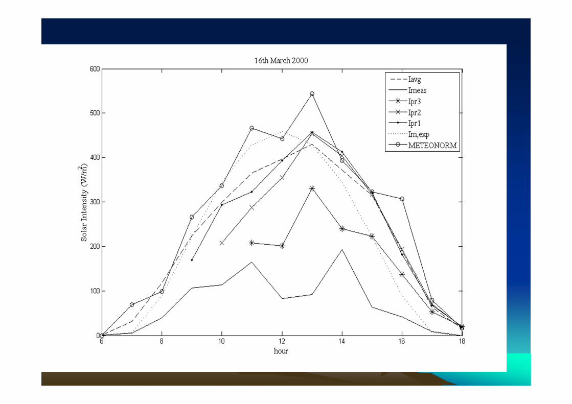
• Mode III of this model gives much better results compared to the other modes, and provides good profiles even in cases where I(h;nj) shows higher degree of fluctuations, as shown for the months November, December, January, February and March.

• The improvement is attributed to the fourth term, which takes into account the second derivative of the difference [Imeas(hi;nj) –Iavg(hi;nj)] for the previous hours.

Conclusions

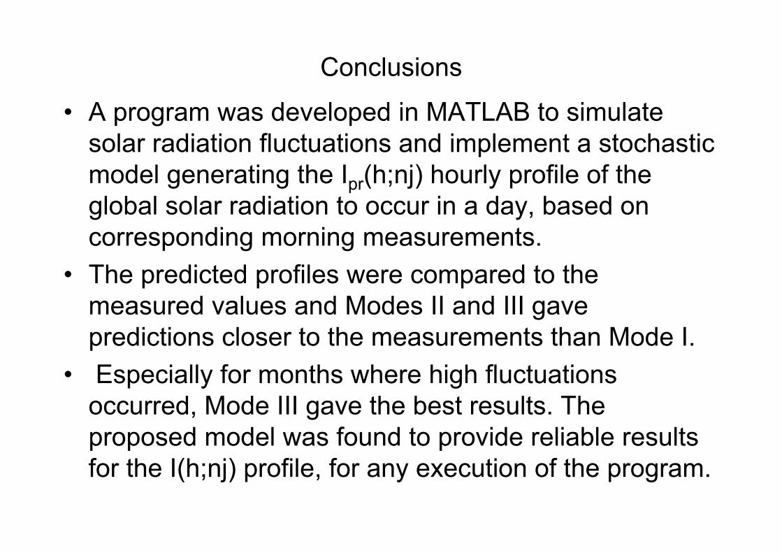
• A program was developed in MATLAB to simulate solar radiation fluctuations and implement a stochastic model generating the Ipr(h;nj) hourly profile of the global solar radiation to occur in a day, based on corresponding morning measurements.

• The predicted profiles were compared to the measured values and Modes II and III gave predictions closer to the measurements than Mode I.

• Especially for months where high fluctuations occurred, Mode III gave the best results. The proposed model was found to provide reliable results for the I(h;nj) profile, for any execution of the program.

• This has a straight impact to the effective prediction of the Power/Energy to be delivered by a PV cell during a day

• which, then, enables the engineer to manage power sources and loads to a much better cost-effective sizing

• ReferencesA stochastic simulation model for reliable PV system sizing providing for solar radiation fluctuationsKaplani, E. , Kaplanis, S. Department of Mechanical Engineering, T.E.I. of Patras, Meg. Alexandrou 1, Koukouli 26334, Patra, GreeceApplied Energy , Volume 97, September 2012, Pages 970-981

Stochastic prediction of hourly global solar radiation for Patra, GreeceKaplanis, S. , Kaplani, E. Mechanical Engineering Dept., T.E.I. of Patras, Meg. Alexandrou 1, Patra, GreeceApplied Energy , Volume 87, Issue 12, December 2010, Pages 3748-3758

A model to predict expected mean and stochastic hourly global solar radiation I(h;nj) valuesKaplanis, S. , Kaplani, E. Renewable Energy Laboratory, T.E.I. of Patra, Meg. Alexandrou 1, Patra 26334, GreeceRenewable Energy, Volume 32, Issue 8, July 2007, Pages 1414-1425

New methodologies to estimate the hourly global solar radiation; Comparisons with existing modelsKaplanis, S.N. Renewable Energy ,Volume 31, Issue 6, May 2006, Pages 781-790